
About Gandhinagar Institute of Technology
289
Gandhinagar Institute of Technology About Gandhinagar Institute of Technology Gandhinagar Institute of Technology is established by Platinum Foundation in 2006. It offers under graduate programs in Mechanical Engineering, Information Technology, Computer Engineering, Electronics and Communication Engineering, Electrical Engineering and Civil Engineering and Post graduate program in MBA (Finance, Human Resource Development, and Marketing) and M.E. in Mechanical Engineering with specialization in Thermal Engineering and Computer Aided Design & Computer Aided Manufacturing. All these programs are approved by AICTE, New Delhi and affiliated to Gujarat Technological University. We have elaborate laboratory facilities and highly motivated and qualified faculty members. We are also arranging technical seminars, conferences, industryinstitute interaction programs, workshops and expert lectures of eminent dignitaries from different industries and various reputed educational institutes. Our students are innovative and have excellent acceptability to latest trends and technologies of present time. Our students have also participated in various technical activities as well as sports activities and have achieved various prices at state level. We have two annual publications, a National level research journal 'GITJournal of Engineering and Technology (ISSN 2249–6157)’ and 'GITa Song of Technocrat' (college magazine). Copyright © 2013 Gandhinagar Institute of Technology, Inc. All rights reserved. Home Trustee Editorial Board Director Message Papers Contact Us
-
Upload
khangminh22 -
Category
Documents
-
view
1 -
download
0
Transcript of About Gandhinagar Institute of Technology

Gandhinagar Institute of Technology
About Gandhinagar Institute of Technology
Gandhinagar Institute of Technology is established by Platinum Foundation in 2006. It offers under graduateprograms in Mechanical Engineering, Information Technology, Computer Engineering, Electronics andCommunication Engineering, Electrical Engineering and Civil Engineering and Post graduate program in MBA(Finance, Human Resource Development, and Marketing) and M.E. in Mechanical Engineering withspecialization in Thermal Engineering and Computer Aided Design & Computer Aided Manufacturing.
All these programs are approved by AICTE, New Delhi and affiliated to Gujarat Technological University. Wehave elaborate laboratory facilities and highly motivated and qualified faculty members. We are also arrangingtechnical seminars, conferences, industryinstitute interaction programs, workshops and expert lectures ofeminent dignitaries from different industries and various reputed educational institutes.
Our students are innovative and have excellent acceptability to latest trends and technologies of present time. Ourstudents have also participated in various technical activities as well as sports activities and have achieved variousprices at state level. We have two annual publications, a National level research journal 'GITJournal ofEngineering and Technology (ISSN 2249–6157)’ and 'GITa Song of Technocrat' (college magazine).
Copyright © 2013 Gandhinagar Institute of Technology, Inc. All rights reserved.
Home Trustee Editorial Board Director Message Papers Contact Us

Gandhinagar Institute of Technology
Shri Hareshbhai B. Rohera,Trustee
Qualifications : B. Com
Background
» Proprietor: Mahadev Steel Suppliers » C/o: Vinayak Steel Syndicate» C/o: Dhiraj Steel Supplier» C/o: Krishna Steel Trader » Owner: National Steel Processor » Trustee: Sai Vasant Ghot Darbar » Trustee: Jai Jhulelal Mandir
Shri Gahanshyambhai V. Thakkar,Trustee
Qualifications : M.A
Background
» Professor at Vivekanand College of Arts, Ahmedabad» Ex. M.L.A., Gujarat Assembaly from Mandal » Trustee of V.M. Thakkar Charitable Trust, Ahmedabad » Manages Muktajeevan Vidhyalaya and BVD High School, Isanpur and Maninagar » Advisor/Member Kankaria Maninagar Nagarik Sahakari Bank » Director Adarsh CoOperative Departmental Stores
Shri Deepakbhai N. Ravani,Trustee
Qualifications :B.Com., LL.B.
Background
» Business
Shri Pravinbhai A. Shah,Trustee
Qualifications : B.A., LL.B.
Background
»President of Zalavad Samaj Jain Seva Trust» Trustee of Vasant » Atma Charitable Trust» Trustee of Rampura Champa Vijya Hospital »Trustee of Shantivan & Ambawadi Jain Sangh »Trustee of Rampura Kelavani Mandal »Trustee of Pampura Panjrapole Trust
Smt Varshaben M. Pandhi,Trustee
Qualifications : B.Com
Background
» Working experience in the field of Insurance and Investment Advisory for about 20 years
Mr. Mahendrabhai Pandhi,Member of Governing Body
Qualifications : B.Com, F.C.A
Background
» Proprietor, M. R. Pandhi & Associates » He has many Indian clients having international presence» His areas of interest are Taxation, Audit, Project Finance and Company Law related matters.» He is one of the memebrs of the study group of 25 Chartered Accountants constituted by WIRC » He has visited many countries like U.A.E., Moratius, Singapore and Africa for his client work.
Home Trustee Editorial Board Director Message Papers Contact Us

Gandhinagar Institute of Technology
Editorial Board
Prof. M N PatelChairman
Principal L.D. College Of Engineering
Navrangpura, Ahmedabad 380 015.
Prof. P K BanikDirector General
Pandit Deendayal Petroleum University Raisan Village, Gandhinagar 382 007.
Dr F S UmarigarPrincipal
Birla Vishvakarma Mahavidhyalaya Vallabhvidyanagar, Anand 388120.
Dr K KotechaDirector
Institute Of Technolgy, Nirma University Sarkhej – Gandhinagar High Way, Ahmedabad 382481.
Dr D J Shah
Principal Sankalchand Patel College of Engineering Nootan Sarva Vidyalaya Kelavani Mandal
S. K Campus, GhandhinagarAmbaji State HighwayVisnagar384315.
Dr C D SankhavaraDean
Faculty of Technology,R K University Kasturbadham Rajkot 360020.
Dr Axay Mehta
Director Gujarat Power Engineering and Research Institute
Near Mevad Toll Booth, Ahmedabad–Mehsana Expressway, Village–Mevad, Dist–Mehsana 382710.
Dr S P Parikh
Principal VVP Engineering College
Virda Vajadi, Kalawad Road, Rajkot, Gujarat360005. Phone : (0281) 2783394, (0281) 2783486.
Dr M S Raval
Professor Dhirubhai Ambani Institute of Information and
Communication Technology Gandhinagar 382 007.
Dr N M Bhatt Director
Home Trustee Editorial Board Director Message Papers Contact Us

Editorial Chief Gandhinagar Institute of Technology Moti Bhoyan, Ta. Kalol Gandhinagar 382721.
Disclaimer
Views expressed in the papers are solely from respective authors. Editorial board has no responsibilityof their authentication.

Gandhinagar Institute of Technology
Message from Director
It is indeed a matter of great pleasure that the sixth issue of our National journal ‘GITJournal of Engineeringand Technology’ is being published with ISSN 2249 – 6157 for sixth successive year. The aim of the journal is topublish peer reviewed research articles in rapidly developing field of engineering and technology. The issue is aresult of imaginative and expressive skill and talent of GIT family. Research papers were invited from theresearcher of all domains of engineering and technology. More than 120 research papers were received. After peerreview, about 50 papers have been selected and published in this issue of the journal. The objectives of impartingadded education, combined with creation, dissemination and application of knowledge, are being met in anintegrated form, to create a synergetic impact. To fulfill its mission in new and powerful ways, each member ofGIT community strives to achieve excellence in every endeavour – be it education, research, consulting or training– by making continuous improvements in curricula and pedagogical tools.
Being a part of GIT, it fills my heart with immense pride and sense of gratitude to state that GIT is wholeheartedly carrying out the chief objective of Educational Process to equip the students as the best professionals.I’m extremely delighted to witness that GIT is working admirably well to prepare the students for their successfulcareer so that they bring crowning glory to themselves and to the institute. Keeping in mind the inevitable need ofproviding educational atmosphere to the students, our institute tries its best to develop their skill and impartknowledge of all domains to enhance their horizons and create more and more opportunities in the field ofTechnology and Research. In the world where change is a buzzword and innovation is the basic necessity, GITteaches its students to ingrain innovativeness as a way of thinking that governs every aspects of life thereby tofoster growth of technology.
During a short span of six years; GIT has accomplished the mission effectively and remarkably well for which itwas established. Institute has been constantly achieving the glory of excellence in the field of curricular, cocurricular and extracurricular activities. Through dedicated efforts of our faculty members and students, it isattempted to translate the vision into action to achieve our mission. “Success is empty if it arrives at the finish linealone. The best reward is to get there surrounded by winners. The more winners you can bring with you the moregratifying the victory you have.” For the fourth consecutive year, an annual technical symposium TechXtreme2013 was successfully organized by the institute. More than 1400 students of various technical institutions acrossthe Gujarat participated in the TechFest. Prizes worth Rs 2 lacs and trophies were given to the winners of total 36events. During the year institute has organized Spoken tutorial on Linux, Latex, Scilab, and Python in associationwith IIT Bombay, seminar on Cisco Networking, Robotics and CAD/CAM workshops for students. The institutehas been successfully organized Debate Competition, Rangoli Competition, Kite Flying competition, Ratri B4Navaratri, and Sports activities. Institute has also arranged two blood donation drives and more than 400 unitswere collected from the students and staff members. Students have also participated and won prizes in varioussports events organized by other Institutions including that of GTU. Students of the institutes won prizes in manytechnical symposiums organized at various engineering colleges of Gujarat. Institute has organized many
industrial visits and expert lectures for the students for supplementing the class room teaching. I am extremely
Home Trustee Editorial Board Director Message Papers Contact Us

industrial visits and expert lectures for the students for supplementing the class room teaching. I am extremelyhappy to mention that throughout the year the faculty members have worked very hard to achieve all kinds ofcurricular, cocurricular and extracurricular activities.
The Institute also puts emphasis on academic development of its faculty members. During the year, 20International and 24 National papers were presented by the faculty members at various conferences organizedacross India. The faculty members were also deputed to attend total 154 seminars/workshops/trainingprograms/symposiums. The institute has organized many state level seminars and workshops on current trends ofEngineering and Management. Spoken tutorial on Linux, Latex, Scilab, and Python in association with IITBombay, CAD/CAM/CAE workshop and AutoCAD 2011 Professional Certificate examination by Auto Desk are afew of them.
Publication of the journal of national level is not possible without wholehearted support of committed andexperienced Trustees of Platinum Foundation Mr. Hareshbhai Rohera, Mr. Ghanshyambhai Thakkar, Mr.Deepakbhai Ravani, Mr. Pravinbhai Shah and Smt. Varshaben M. Pandhi. I take an opportunity to express mydeep feelings of gratitude to all the trustees of Platinum Foundation and Mr. Mahendrabhai Pandhi, member ofGoverning body of the trust for their constant motivational support.
It’s my privilege to compliment the staff members and the students for showing high level of liveliness throughoutthe year. Mere thanks in a few words are not enough to offer my sincere appreciation and congratulate the teamof the ‘GITJournal of Engineering and Technology’ for their untiring effort to give final shape to the sixth issueof the journal. I am heartily thankful to each and every member of the institute for providing active participationand best motivational support in the thorough development of the institute.
Dr N M Bhatt Director

Gandhinagar Institute of Technology
Mechanical EngineeringSr.No. Paper Title Author Name Institute Detail Author E_Mail Id CoAuthors Name
1Heat Transfer Coefficient andPressure Drop over InlinePitch Variation using CFD
Prof.Nirav R. BhavsarParul Institute ofEngineering &Technology
[email protected] Mr.Rupen R.Bhavsar
2 Thermal Analysis of LiquidNitrogen Storage Vessel
Prof. Vimalkumar PSalot
L.J.Institute ofEngineering &Technology,Ahmedabad
3Employment of AdvancedMaterials for Boilers andSteam Turbines
Prof.Chintan T.Barelwala
Gandhinagar Instituteof Technology [email protected]
4
Effect of target frequency, biasvoltage, bias frequency anddeposition temperature ontribological properties ofpulsed DC CFUBM sputteredTiN coating
Prof. Arpan P.Shah BITS EducationCampus, Varnama [email protected] Dr. Soumitra Paul
5
Prevention Methods forreduce welding leakages inAluminium using TIG andMIG welding
Prof.Vyomesh R Buch BITS EducationCampus, Varnama [email protected] Prof.K. Baba.Pai
6 Parametric Study of TubeHydroforming Process
Prof.Vijaykumar RParekh
Shri S’ad VidyaMandal Institute OfTechnology
[email protected]. C. Patel
Prof. J. R. Shah
7
Effect of Applying HPC JETin Machining of 42CrMo4Steel Using Uncoated CarbideInserts
Prof.Mayur S Modi
Shree SwamiAtmanand SaraswatiInstitute ofTechnology, SURAT
[email protected] Mr.Sandip G. Patel
8Experimental analysis of heatpump used for simultaneousheating and cooling utilities
Mr. Rahulbhai P PatelShri S’ad VidyaMandal Institute OfTechnology
[email protected] Dr. Ragesh GKapadia
9Design and Analysis of a HighPressure vessel using ASMEcode
Prof. Mitesh Mungla Gandhinagar Instituteof Technology [email protected]
Mr.K N Srinivasan
Prof. V R Iyer
10
Studies on effect of processparameters on tensileproperties and failurebehavior of friction stirwelding of Al alloy
Prof. Bhavesh R.RanaIndus University,Rancharda Via ThaltejAhemedabad
[email protected]. L.V.Kasmble
Dr.S.N.Soman
11
Review on The Energy SavingsAnd Economic Viability OfHeat Pump Water Heaters InThe Residential Sectors – AComparison With Solar WaterHeating System
Mr.Vinod P Rajput Gandhinagar Instituteof Technology [email protected]
Mr.Ankit K. Patel
Prof.Nimesh Gajjar
12Effect of PWHT soaking timeon Mechanical & metallurgicalproperties of 9Cr1MoV steel
Mr. Naishadh PatelIndus University,Rancharda Via ThaltejAhemedabad
[email protected]. Pavan Maniar
Prof. M.N. Patel
13Heat Transfer Coefficient andPressure Drop over StaggeredPitch Variation using CFD
Prof.Nirav R. BhavsarParul Institute ofEngineering &Technology
[email protected] Mr. Rupen R.Bhavsar
14
Application of Porous MediumTechnology to InternalCombustion Engine forHomogeneous Combustion AReview
Prof.Ratnesh TParmar
L D College ofEngineering [email protected] Prof.Vimal Patel
15
Fabrication andCharacterization of CastAluminium Fly AshComposite
Dr. Vandana J RaoThe MaharajaSayajirao Universityof Baroda
[email protected] N.Panchal
Ms.Sonam M. Patel
Home Trustee Editorial Board Director Message Papers Contact Us

16 Review on CO2 Laser CuttingProcess Parameter
Prof. Dhaval P Patel Gandhinagar Instituteof Technology
17 Effect of Silicon addition inLM25 Aluminium Alloy Prof. Hitesh H. Patel Gandhinagar Institute
of Technology [email protected]
18Numerical Investigation ofFlow over cylinder for thestudy of different flow pattern
Prof. Hardik R Gohel Gandhinagar Instituteof Technology [email protected]
Prof. Absar MLakdawala
19Development of Test Rig forVibration Monitoring ofBearing
Prof. Amit R Patel Gandhinagar Instituteof Technology [email protected]
20
Secondary Refrigerant Systemfor Water Ice CandyManufacturing Process withCalcium Chloride Brine
Prof. Keyur C Patel Gandhinagar Instituteof Technology [email protected]
Dr. Vikas J.Lakhera
21
Development of Typicalsample holder with Cryostatfor the Measurement of HallEffect and MagneticSusceptibility at LN2Temperature.
Mr. Shaival R Parikh L D College ofEngineering [email protected] Prof. Hardik
Shukla
22
A Review on Heatpipe Ovenfor Plasma WakefieldAccelerator (PWFA)Experiment
Mr. Milind A. Patel Gandhinagar Instituteof Technology [email protected] Prof. Krunal Patel
23
Cryostat for Measurement ofThermal Conductivity,Electrical Resistivity andThermoelectric Power ofLaBa2Cu3O7δ
Mr. Ruchir Parikh L D College ofEngineering [email protected]
Dr. J M Patel
24
Enhancement in mappingcapability of Feature Replacecommand in NX CADsoftware
Mr.Pankaj Sharma Nirma University [email protected] Deshmukh
Prof.Reena trivedi
25 Waste Heat Recovery fromVCR Systems – A Review Mr. Ankit Patel Gandhinagar Inst. of
Technology [email protected]
Dr N M Bhatt
Prof. Nimesh Gajjar

Gandhinagar Institute of Technology
Computer ScienceSr.No. Paper Title Author Name Institute Detail Author E_Mail Id CoAuthors Name
1 Skinput Technology Mr. Nirav K. Shah
Shree swaminarayancollege of computerscience, Bhavnagar (Affiliated to M.K.Bhavnagar University,Bhavnagar)
[email protected]. Madhav K. Dave
Mr. Parag B. Makwana
2
Privacy Preserving DataStream Classfication: Anapproach Using MOAFramework
Prof. Kirankumar SPatel
Gandhinagar Instituteof Technology [email protected]
3 Comparative Study of WebPage Classification Techniques
Prof. Anirudhdha MNayak
Gandhinagar Instituteof Technology [email protected]
4
Explain Use Case Point EffortEstimation Method Taking theCase of University RegistrationSystem Use Case Diagram
Prof. Svapnil Vakharia Gandhinagar Instituteof Technology [email protected]
5Essential Aspects of Security,Privacy and Challenges inCloud
Ms. Leena B.Patel Gandhinagar Instituteof Technology [email protected]
6 System Description Formationfor University Blackboard Tool
Prof. Birendrasinh KZala
Gandhinagar Instituteof Technology [email protected]
7 A Survey On RecommendingTags Methodologies Prof. Brinda R. Parekh Gandhinagar Institute
of Technology [email protected]
8
Study and Review of VariousIdentity and PrivacyManagement Techniques inConsumer Cloud Computing
Ms. Archana NMahajan
SSBT’S College Of Enggand Technology [email protected] Mr. Sandip S. Patil
Home Trustee Editorial Board Director Message Papers Contact Us

Gandhinagar Institute of Technology
Electronics & CommunicationSr.No. Paper Title Author Name Institute Detail Author E_Mail Id CoAuthors Name
1
Performance Analysis of a SubOptimum Transmit AntennaSelection Scheme with MPSK andMQAM Constellations.
Prof. Jatin M.Chakravarti
GandhinagarInstitute OfTechnology
[email protected] Prof. Mitul P.Maniar
2
Comparision of Different EdgeBased Active Contour Models andTheir Solution for ImageSegmentation
Prof. DhavalRajeshbhai Sathawara
U.V. Patel College ofEngineering, GanpatUniversity, Kherva
[email protected]. Margam K.Suthar
Mr.Bharat P. Solanki
3BER Performance of EqualizedSignal in Wireless CommunicationArchitecture of Smart Grid
Prof. Vineeta NishadGandhinagarInstitute ofTechnology
[email protected] Prof. JitendraThathagar
4 High Speed CMOS ComparatorDesign
Prof. Megha MauleshDesai
GandhinagarInstitute ofTechnology
5Simulation & Performance Analysisof DVBT System Using EfficientWireless Channels
Prof. Nirali KotakGandhinagarInstitute ofTechnology
6
Technique for Non DistractiveQuality Evaluation of CuminumCyminum L(Cumin) Seeds UsingColorization
Prof. Jalpa PatelGandhinagarInstitute ofTechnology
7PortableWirelessVibrationMonitoringSystemfor Measurement
Prof. Pratik GohelGandhinagarInstitute ofTechnology
[email protected]. Gunjan Jani
Prof. Dhiren Vaghela
Home Trustee Editorial Board Director Message Papers Contact Us

GIT-Journal of Engineering and Technology (Sixth volume, 2013, ISSN 2249 – 6157)
Abstract—This is a technology that appropriates the human
body for acoustic transmission, allowing the skin to be used as an
input surface. In particular, resolves the location of finger tips on
the arm and hand by analyzing mechanical vibrations that
propagate through the body. We collect these signals using a
novel array of sensors worn as an armband. This approach
provides an always available, naturally portable, and on-body
finger input system. We assess the capabilities, accuracy and
limitations of our technique through a two-part, twenty-
participant user study. So in a few years time, with Skinput,
computing is always available: A person might walk toward their
home, tap their palm to unlock the door and then tap some virtual
buttons on their arms to turn on the TV and start flipping
through channels.
Index Terms—Microsoft Technology, Skinput, Acoustic Handson
I. INTRODUCTION
he primary goal of Skinput is to provide an always
available mobile input system - that is, an input system
that does not require a user to carry or pick up a device. A
number of alternative approaches have been proposed that
operate in this space. Techniques based on computer vision are
popular these, however, are computationally expensive and
error prone in mobile scenarios (where, e.g., non-input optical
flow is prevalent). Speech input is a logical choice for always-
available input, but is limited in its precision in unpredictable
acoustic environments, and suffers from privacy and
scalability issues in shared environments. Other approaches
have taken the form of wearable computing.
This typically involves a physical input device built in a
form considered to be part of one's clothing. For example,
glove-based input systems allow users to retain most of their
natural hand movements, but are cumbersome, uncomfortable,
and disruptive to tactile sensation. Post and Orth present a
"smart fabric" system that embeds sensors and conductors into
abric, but taking this approach to always-available input
necessitates embedding technology in all clothing, which
would be prohibitively complex and expensive. The Sixth
Sense project proposes a mobile, always available input/output
capability by combining projected information with a color-
marker-based vision tracking system. This approach is
feasible, but suffers from serious conclusion and accuracy
limitations. For example, determining whether, a finger has
tapped a button, or is merely hovering above it, is
extraordinarily difficult.
II. BIO-SENSING
Skinput leverages the natural acoustic conduction properties
of the human body to provide an input system, and is thus
related to previous work in the use of biological signals for
computer input. Signals traditionally used for diagnostic
medicine, such as heart rate and skin resistance, have been
appropriated for assessing a user's emotional state. These
features are generally subconsciously driven and cannot be
controlled with sufficient precision for direct input. Similarly,
brain sensing technologies such as electroencephalography
(EEG) & functional near-infrared spectroscopy (fNIR) have
been used by HCI researchers to assess cognitive and
emotional state; this work also primarily looked at involuntary
signals. In contrast, brain signals have been harnessed as a
direct input for use by paralyzed patients, but direct brain
computer interfaces (BCIs) still lack the bandwidth required
for everyday computing tasks, and require levels of focus,
training, and concentration that are incompatible with typical
computer interaction.
Skinput Technology
Mr. Nirav K. Shah, Mr. Madhav K. Dave, Mr. Parag B. Makwana
( [email protected], [email protected], [email protected] )
T

GIT-Journal of Engineering and Technology (Sixth volume, 2013, ISSN 2249 – 6157)
Fig 1.0Hand sensing
There has been less work relating to the intersection of finger
input and biological signals. Researchers have harnessed the
electrical signals generated by muscle activation during normal
hand movement through electromyography (EMG). At present,
however, this approach typically requires expensive
amplification systems and the application of conductive gel for
effective signal acquisition, which would limit the
acceptability of this approach for most users. The input
technology most related to our own is that of Amen to et al
who placed contact microphones on a user's wrist to assess
finger movement. However, this work was never formally
evaluated, as is constrained to finger motions in one hand.
The Hambone system employs a similar setup, and through an
HMM, yields classification accuracies around 90% for four
gestures (e.g., raise heels, snap fingers). Performance of false
positive rejection remains untested in both systems at present.
Moreover, both techniques required the placement of sensors
near the area of interaction (e.g., the wrist), increasing the
degree of invasiveness and visibility. Finally, bone conduction
microphones and headphones - now common consumer
technologies - represent an additional bio-sensing technology
that is relevant to the present work. These leverage the fact
that sound frequencies relevant to human speech propagate
well through bone.
Bone conduction microphones are typically worn near the ear,
where they can sense vibrations propagating from the mouth
and larynx during speech. Bone conduction headphones send
sound through the bones of the skull and jaw directly to the
inner ear, bypassing transmission of sound through the air and
outer ear, leaving an unobstructed path for environmental
sounds.
III ACOUSTIC INPUT
Our approach is also inspired by systems that leverage acoustic
transmission through(non-body) input surfaces. Paradise et al.
measured the arrival time of a sound at multiple sensors to
locate hand taps on a glass window. Ishii et al. use a similar
approach to localize ball hitting a table, for computer
augmentation of a real-world game. Both of these systems use
acoustic time-of-flight for localization, which we explored, but
found to be insufficiently robust on the human body, leading to
the fingerprinting approach described in this paper frequencies
propagate more readily through bone than through soft tissue,
and bone conduction carries energy over larger distances than
soft tissue conduction. While we do not explicitly model the
specific mechanisms of conduction, or depend on these
mechanisms for our analysis, we do believe the success of our
technique depends on the complex acoustic patterns that result
from mixtures of these modalities. Similarly, we also believe
that joints play an important role in making tapped locations
acoustically distinct. Bones are held together by ligaments, and
joints often include additional biological structures such as
fluid cavities. This makes joints behave as acoustic filters. In
some cases, these may simply dampen acoustics; in other
cases, these will selectively attenuate specific frequencies,
creating location specific acoustic signatures.
IV. SENSING
To capture the rich variety of acoustic information described
in the previous section, we evaluated many sensing
technologies, including bone conduction microphones,
conventional microphones coupled with stethoscopes and
accelerometers. However, these transducers were engineered
for very different applications than measuring acoustics
transmitted through the human body. As such, we found them
to blacking in several significant ways. Foremost, most
mechanical sensors are engineered to provide relatively flat
response curves over the range of frequencies that is relevant
to our signal. This is a desirable property for most applications
where a faithful representation of an input signal uncolored by
the properties of the transducer is desired. However, because
only a specific set of frequencies is conducted through the arm
in response to tap input, a flat response curve leads to the
capture of irrelevant frequencies and thus to a high signal- to-
noise ratio. While bone conduction microphones might seem a
suitable choice for Skinput . These devices are typically
engineered for capturing human voice, and filter out energy
below the range of human speech(whose lowest frequency is
around 85Hz). Thus most sensors in this category were not
especially sensitive to lower-frequency signals (e.g., 25Hz),
which we found in our empirical pilot studies to be vital in
characterizing finger taps. To overcome these challenges, the
idea of a single sensing element with a flat response curve, to
an array of highly tuned vibration sensors was dropped.
Specifically, employed a small, cantilevered piezo films
MiniSense100, Measurement Specialties, Inc.).By adding
small weights to the end of the cantilever, we are able to alter
the resonant frequency, allowing the sensing element to be
responsive to a unique, narrow, low-frequency band of the
acoustic spectrum. Adding more mass lowers the range of
excitation to which sensor responds; we weighted each
element such that it aligned with particular frequencies that
pilot studies showed to be useful in characterizing bio-acoustic
input. Figure shows the response curve for one of our sensors,

GIT-Journal of Engineering and Technology (Sixth volume, 2013, ISSN 2249 – 6157)
tuned to a resonant frequency of 78Hz. The curve shows a
~14dB drop-off ±20Hz away from the resonant frequency.
Additionally, the cantilevered sensors were naturally
insensitive to forces parallel to the skin (e.g., shearing motions
caused by stretching). Thus, the skin stretch induced by many
routine movements (e.g., reaching for a doorknob) tends to be
attenuated. However, the sensors are highly responsive to
motion perpendicular to the skin plane perfect for capturing
transverse surface waves and longitudinal waves emanating
from interior structures Finally, our sensor design is relatively
inexpensive and can be manufactured in a very small form
factor (e.g., MEMS), rendering it suitable for inclusion in
future mobile devices (e.g., an arm-mounted audio player).
ARMBAND PROTOTYPE
In five sensing elements, incorporated into an armband form
factor. The decision to have two sensor packages was
motivated by our focus on the arm for input. In particular,
when placed on the upper arm (above the elbow), we hoped to
collect acoustic information from the fleshy bicep area in
addition to the firmer area on the underside of the arm, with
better acoustic coupling to the Hummers the main bone that
runs from shoulder to elbow. When the sensor was placed
below the elbow, on the forearm, one package was located
near the Radius , the bone that runs from the lateral side of the
elbows the thumb side of the wrist, and the other near the Ulna
, which runs parallel to this on the medial side of the arm
closest to the body. Each location thus provided slightly
different acoustic coverage and information, helpful in
disambiguating input location. Based on pilot data collection,
we selected a different set of resonant frequencies for each
sensor package. We tuned the upper sensor package to be
more sensitive to lower frequency signals, as these were more
prevalent in fleshier areas. Conversely, we tuned the lower
sensor array to be sensitive to higher frequencies, in order to
better capture signals transmitted though (denser)bones.
PROCESSING
In this prototype system, each channel was sampled at 5.5kHz,
a sampling rate that would be considered too low for speech or
environmental audio, but was able to represent the relevant
spectrum of frequencies transmitted through the arm. This
reduced sample rate (and consequently low processing
bandwidth) makes our technique readily portable to embedded
processors. For example, the ATmega168 processor employed
by the Adriano platform can sample analog readings at 77 kHz
with no loss of precision, and could therefore provide the full
sampling power required for Skinput (55 kHz total).Data was
then sent from our thin client over a local socket to our
primary application, written in Java. This program performed
three key functions. First, it provided a live visualization of the
data from our ten sensors, which was useful in identifying
acoustic features. Second, it segmented inputs from the
DataStream into independent instances (taps). Third, it
classified these input instances. The audio stream was
segmented into individual taps using an absolute exponential
average of all ten channels. When an intensity threshold was
exceeded, the program recorded the timestamp as a potential
start of a tap. If the intensity did not fall below a second,
independent closing‖ threshold between 100ms and 700ms
after the onset crossing (a duration we found to be the common
for finger impacts), the event was discarded. If start and end
crossings were detected that satisfied these criteria, the
acoustic data in that period (plus a 60ms buffer on either
end)was considered an input event .Although simple, this
heuristic proved to be highly robust, mainly due to the extreme
noise suppression provided by sensing approach. After an
input has been segmented, the waveforms are analyzed. The
highly discrete nature of taps (i.e. point impacts) meant
acoustic signals were not particularly expressive over time
(unlike gestures, e.g., clenching of the hand). Signals simply
diminished in intensity overtime. Thus, features are computed
over the entire input window and do not capture any temporal
dynamics. Brute force machine learning approach is employed,
computing 186 features in total, many of which are derived
combinatorial. For gross information, the average amplitude,
standard deviation and total(absolute) energy of the waveforms
in each channel (30 features) is included. From these, average
amplitude ratios between channel pairs (45 features) are
calculated. An average of these ratios (1 feature) is also
included. A 256-point FFT for all ten channels, although only
the lower ten values are used (representing the acoustic power
from 0Hz to 193Hz), yields100 features. These are normalized
by the highest-amplitude FFT value found on any channel.
Also the center of mass of the power spectrum within the same
0Hz to 193Hz range for each channel, a rough estimation of
the fundamental frequency of the signal displacing each
sensor(10 features) are included. Subsequent feature selection
established the all-pairs amplitude ratios and certain bands of
the FFT to be the most predictive features. These 186 features
are passed to a Support Vector Machine (SVM) classifier. A

GIT-Journal of Engineering and Technology (Sixth volume, 2013, ISSN 2249 – 6157)
full description of SVMs is beyond the scope of this paper.
Our software uses the implementation provided in the Weka
machine learning toolkit. It should be noted, however, that
other, more sophisticated classification techniques and features
could be employed. Thus, the results presented are to be
considered a baseline. Before the SVM can classify input
instances, it must first be trained to the user and the sensor
position. This stage requires the collection of several examples
for each input location of interest. When using Skinput to
recognize live input, the same 186 acoustic features are
computed on-the fly for each segmented input. These are fed
into the trained SVM for classification. Once an input is
classified, an event associated with that location is instantiated.
Any interactive features bound to that event are fired.
CONCLUSION
We conclude approach to appropriating the human body as an
input surface. It describes a novel, wearable bio-acoustic
sensing array that we built into an armband in order to detect
and localize finger taps on the forearm and hand. These
include single-handed gestures, taps with different parts of the
finger, and differentiating between materials and objects. We
conclude with descriptions of several prototype applications
that demonstrate the rich design space we believe
Skinput enables.
References
[1] Harrison Chris, ― Skinput:Appropriating the body as an input surface‖
ACM conference 2010.
[2] Hope, Dan ―Skinput turns body into touch screen interface‖
[3] W. D. Doyle, ―Magnetization reversal in films with biaxial anisotropy,‖
in 1987 Proc. INTERMAG Conf., pp. 2.2-1–2.2-6.
[4] Hornyak Tom, ―Turn your arm into a phone with Skinput‖

GIT-Journal of Engineering and Technology (Sixth volume, 2013, ISSN 2249 – 6157)
Abstract— Data stream can be conceived as a continuous and
changing sequence of data that continuously arrive at a system to
store or process. Examples of data streams include computer
network traffic, phone conversations, web searches and sensor
data. These data sets need to be analyzed for identifying trends
and patterns which help us in isolating anomalies and predicting
future behavior. However, data owners or publishers may not be
willing to exactly reveal the true values of their data due to
various reasons, most notably privacy considerations. Hence,
some amount of privacy preservation needs to be done on the data
before it can be made publicly available. To preserve data privacy
during data mining, the issue of privacy- preserving data mining
has been widely studied and many techniques have been
proposed. However, existing techniques for privacy-preserving
data mining are designed for traditional static databases and are
not suitable for data streams. So the privacy preservation issue of
data streams mining is a very important issue. This paper is about
describing a Method which extends the process of data
perturbation on dataset to achieve privacy preservation. We can
compare the classification characteristics in terms of less
information loss, response time, and more privacy gain so get
better accuracy of data stream algorithms
Index Terms— Decision trees, Hoeffding Tree
I. INTRODUCTION
In the field of information processing, data mining refers to
the process of extracting the useful knowledge from the large
volume of data. There is plenty of area where the data
mining is widely applied such as Healthcare which includes
Medical diagnostics, insurance claims analysis, drug
development, Business, finance, education, sports and
gambling, insurance, stock market, retail, telecommunication,
transportation etc. Widely used data mining techniques in such
area of application includes Clustering of data, Classification,
Regression Analysis, Association rule / pattern mining.
The data stream paradigm has recently emerged in
response to the continuous data problem [2]. Mining data
streams is concerned with extracting knowledge structures
represented in models and patterns in non-stopping,
continuous streams (flow) of information. Algorithms written
for data streams can naturally cope with data sizes many times
greater than memory, and can extend to challenging real-time
applications not previously tackled by machine learning or
data mining. The assumption of data stream processing is that
training examples can be briefly inspected a single time only,
that is, they arrive in a high speed stream, and then must be
discarded to make room for subsequent examples. The
algorithm processing the stream has no control over the order
of the examples seen, and must update its model incrementally
as each example is inspected. An additional desirable property,
the so-called anytime property, requires that the model is ready
to be applied at any point between training examples.
Traditional data mining approaches have been used in
applications that have persistent data available and generated
learning models are static in nature. Since whole data available
before we make it available to our machine learning algorithm,
statistical information of the data distribution can be known in
advance. The task performed by the mining process are
centralized, produce the static learning model. There is no way
of incremental processing of data if the available larger dataset
are sampled in order to accommodate with the memory which
smaller in size with respect to larger size of data. For each
sample the learning model start processing from the scratch.
There is no way of intermediately analysis of the result.
But nowadays, in the field of information processing, an
emergence of applications that do not fit this data model [3]
Instead, information naturally occurs in the form of a sequence
(stream) of data values. A data stream is a real-time,
continuous, and ordered sequence of items. It is not possible to
control the order in which items arrive, nor feasible to locally
store a stream in its entirety. Likewise, queries over streams
run continuously over a period of time and incrementally
return new results as new data arrive.
II. PRIVACY CONSERN
Examples of data streams include computer network traffic,
phone conversations, web searches and sensor data. These data
sets need to be analyzed for identifying trends and patterns
which help us in isolating anomalies and predicting future
behavior. However, data owners or publishers may not be
willing to exactly reveal the true values of their data due to
various reasons, most notably privacy considerations. Hence,
some amount of privacy preservation needs to be done on the
data before it can be made publicly available. The
interpretation of data is important and it is conjoined with the
Privacy-Preserving Data Stream Classification:
An approach using MOA framework
Mr.Kirankumar Patel
I

GIT-Journal of Engineering and Technology (Sixth volume, 2013, ISSN 2249 – 6157)
need to maintain privacy using suitable algorithms. Various
methods have been proposed for this purpose like data
perturbation and encryption and masking, k-anonymity,
association rule mining etc. However these methods cannot be
applied on data streams directly. Moreover, in data streams
applications, there is a need to offer strong guarantees on
maximum allowed delay between incoming data and its
anonymous output. Also less data losses and more privacy
gain.
Verykios et al. [4] classified privacy- preserving data
mining techniques based on five dimensions, which are data
distribution, data modification, data mining algorithms, data or
rule hiding, and privacy preservation, respectively.
In the dimension of data distribution, some approaches
have been proposed for centralized data and some for
distributed data. Du and Zhan [5] utilized the secure union,
secure sum and secure scalar product to prevent the original
data of each site from revealing during the mining process. At
the end of the mining process, every site will obtain the final
result of mining the whole data. The disadvantage is that the
approach requires multiple scans of the database and hence is
not suitable for data streams, which flows in fast and requires
immediate response.
In the dimension of data modification, the confidential
values of a database to be released to the public are modified
to preserve data privacy. Adopted approaches include
perturbation, blocking, aggregation or merging, swapping, and
sampling. Agrawal and Srikant [6] used the random data
perturbation technique to protect customer data and then
constructed the decision tree. For data streams, because data
are produced at different time, not only data distribution will
change with time, but also the mining accuracy will decrease
for modified data.
Privacy preservation techniques can be classified into three
categories, which are heuristic-based techniques,
cryptography-based techniques, and reconstruction-based
techniques. From the review of previous research, we can see
that existing techniques for privacy-preserving data mining are
designed for static databases with an emphasis on data
security. These existing techniques are not suitable for data
streams.
In [7], considered the classification problem where the
training data are several private data streams. Joining all
streams violates the privacy constraint of such applications and
suffers from the blow- up of join. In that presented a solution
based on Naive Bayesian Classifiers. The main idea is rapidly
obtaining the essential join statistics without actually
computing the join. With this technique, they can build exactly
the same Naive Bayesian Classifier as using the join stream
without exchanging private information. The processing cost is
linear in the size of input streams and independent of the join
size. But there are some drawback related time and data arrival
rate that is Having a much lower processing time per input
tuple, the proposed method is able to handle much higher data
arrival rate and deal with the general many-to-many join
relationships of data streams.
In [8], proposed the method for privacy-preserving
classification of data streams, which consists of two stages:
date streams pre-processing and data streams mining. In the
stage of data streams pre-processing, proposed the data
streams pre-processing (DSP) algorithm to perturb data
streams. Experimental results of security measurement showed
that the DSP algorithm has higher .security. Experimental
results of data error measurement showed that DSP algorithm
has less data error. In the stage of data streams mining,
proposed the WASW algorithm to mine perturbed data
streams. Experiment results of accuracy measurement showed
that the error rate of the VFDT algorithm increases constantly
along with continuous arrival of the data stream but the error
rate of the WASW algorithm is kept under the predetermined
threshold value. Therefore, the WASW algorithm has higher
accuracy. In conclusion, the PCDS method not only can
preserve data privacy but also can mine data streams
accurately.
III. RELATED WORK
Motivated by the privacy concerns on data mining tools, a
research area called privacy-preserving data mining. The
initial idea of it was to extend traditional data mining
techniques to work with the stream data modified to mask
sensitive information. The key issues were how to modify the
data and how to recover the data stream mining result from the
modified data. The solutions were often tightly coupled with
the data stream mining algorithms under consideration.
In this paper introduce a new data perturbation algorithm for
perturb the dataset. And then apply the Hoeffding tree
algorithm on perturbed dataset. Two step process: in the first
step applying the perturbation algorithm on dataset. In the
second step applying the Hoeffding tree algorithm on that
perturbed dataset.
The goal is to transform a given data set D into modified
version D’ that satisfies a given privacy requirement and
preserves as much information as possible for the intended
data analysis task.
We can compare the classification characteristics in terms of
less information loss, response time, and more privacy gain so
get better accuracy of different data stream algorithms against
each other and with respect to the following benchmarks:
• Original, the result of inducing the classifier on
unperturbed training data without randomization.
• Randomized, the result of inducing the classier on
perturbed data (Perturbation based methods for
privacy preserving perturb individual data values or
the results of queries by swapping, condensation, or
adding noise.) but without making any corrections
for randomization.
IV. DATA PURTURBATION ALGORITHM
The stage of data streams pre-processing uses perturbation
algorithm to perturb confidential data. Users can flexibly

GIT-Journal of Engineering and Technology (Sixth volume, 2013, ISSN 2249 – 6157)
adjust the data attributes to be perturbed according to the
security need. Therefore, threats and risks from releasing data
can be effectively reduced.
----------------------------------------------------------------------
Algorithm: Data Perturbation (perturbation algorithm use for
perturb confidential data and provide Data Privacy)
Input: An Original Dataset S (.ARFF or .CSV file)
Output: A perturbed Dataset S’ (perturb dataset .ARFF or
.CSV file)
Algorithm Step:
1. Read Original Dataset S file.(fie extension must be
.ARFF or .CSV file)
2. Display set of attribute name and total number of
attribute that are in the dataset S (.ARFF or .CSV
file). Also With data types of that attribute
3. Display total number of tuples in dataset S.
4. Select sensitive attribute from step 3.
5. If suppose selected attribute is F* then
a) Assign window to F* attribute (window store
received dataset according to order of arrival)
b) Suppose size of window is W(selection of size at
run time) than it contain only W tuples of
selected attribute F* values
c) Then find mean of that W tuples that are in the
window.
d) Replace first tuple of window by mean that we
find in above step 5c.
e) Remaining tuples are as it is.
f) Apply Sliding window means remove first tuple
of window and insert next tuple from original
dataset to end of window.so sliding window
size remain same.
6. Again find mean of modified window so go to step 5(a)
to 5(f) until all the values of attribute F* is changed.
7. Then modified dataset save in .CSV or .ARFF file.
Also called perturbed dataset S’.
----------------------------------------------------------------------
Fig.1 Data Perturbation Algorithm
See following sample table I sample dataset, in this table
selected attribute F* is Salary, and table contain before and after perturbation values.so compare both salary attribute those contain salary attribute original data and perturbed data.
TABLE I SAMPLE DATASET
Record
No.
Age Education
level
Salary
(Before
perturbation)
Salary
(After
perturbation)
1 23 15 53 57.5
2 31 14 55 52.0
3 33 18 62 57.5
4 36 11 49 52.0
5 42 15 63 62.0
6 48 18 70 71.5
See Figure 2 and following step 1 to step 3 are for basic concept of sliding window.
Fig. 2 sliding window concepts
1. Apply window to selected attribute F*( here selected
attribute is Attribute salary(before perturbation) contain
window size is 4 Tuple1 to tuple4)
2. Find mean of this attribute (mean of tuple1 to tuple4) and
replace first value of window that is 53 by mean. And
remaining tuple values are as it is.
3. Suppose mean is 57.5 than replace first value from
window by mean values 57.5. And remaining as it is.
And sliding window by 1 tuple so new window is from
tuple2 to tuple5. Then again find modified wind mean
and replace until all values of attribute salary(before
perturbation) is change and we save in new column
that is salary(after perturbation) .
V. CLASSIFICATION ALGORITHM: HOEFFDING TREE
Before starting a Hoeffding algorithm, first of all we define classification problem is a set of training examples of the form (x, y), where x is a vector of d attributes and y is a discrete class label. Our goal is to produce from the examples a model y=f(x) that predict the classes y for future examples x with high accuracy. Decision tree learning is one of the most effective classification methods. a Decision tree is learned by recursively replacing leaves by test nodes, starting at the root. Each node contains a test on the attributes and each branch from a node corresponds to a possible outcome of the test and each leaf contains a class prediction. All training data stored in main memory so it’s expensive to repeatedly read from disk when learning complex trees so our goal is design decision tree learners than read each example at most once, and use a small constant time to process it.
So key observation is find the best attribute at a node. So for that consider only small subset of training examples that pass through that nodes. Choose the root attribute. Then expensive examples are passed down to the corresponding leaves, and used to choose the attribute there, and so on recursively. so use Hoeffding bound to decide, how many examples are enough at each node???

GIT-Journal of Engineering and Technology (Sixth volume, 2013, ISSN 2249 – 6157)
Consider a random variable a contain range is R. suppose
we have n observation of a. so find mean of a ( ).so Hoeffding
bound states that “with probability 1-δ, the true mean of a is at
least - ε. where Hoeffding bound ε
(1)
-----------------------------------------------------------------
Algorithm Hoeffding tree induction algorithm.
1: HT be a tree with a single leaf (the root)
2: for all training examples do
3: Sort example into leaf l using HT
4: Update sufficient statistics in l
5: Increment nl , the number of examples seen at l
6: if nl mod Nmin = 0 and examples seen at l not all
of same Class then
7: Compute l (Xl) for each attribute
8: Let Xa be attribute with highest l
9: Let Xb be attribute with second-highest l
10: Compute Hoeffding bound
11: if Xa ≠ XØ; and ( l (Xa) - l (Xb) > ε or ε < τ )
then
12: Replace l with an internal node that splits on Xa
13: for all branches of the split do
14: Add a new leaf with initialized sufficient
statistics
15: end for
16: end if
17: end if
18: end for
-----------------------------------------------------------------
Figure 4 Hoeffding tree algorithm [9]
In Line 1 initializes the tree data structure, which starts out as a single root node. Lines 2-18 form a loop that is performed for every training example. Every example is filtered down the tree to an appropriate leaf, depending on the tests present in the decision tree built to that point (line 3). This leaf is then updated (line 4)—each leaf in the tree holds the sufficient statistics needed to make decisions about further growth. The sufficient statistics that are updated are those that make it possible to estimate the information gain of splitting on each attribute. Line 5 simply points out that nl is the example count at the leaf, and it too is updated. Technically nl can be computed from the sufficient statistics. Lines 7-11 perform the test described in the previous section, using the Hoeffding bound to decide when a particular attribute has won against all of the others. G is the splitting criterion function
(information gain) and is its estimated value. In line 11 the
test for XØ, the null attribute, is used for pre-pruning. The test involving τ is used for tie-breaking. If an attribute has been selected as the best choice, lines 12-15 split the node, causing the tree to grow. [9]
VI. EXPERIMENT SETUP AND RESULT
We have conducted experiments to evaluate the
performance of data perturbation method. We choose
generated Database. Generate a dataset from MOA (massive
online analysis) Framework [11]. And use the Agraval dataset
generator. We use WEKA (Waikato Environment for
Knowledge Analysis) [10] software that is integrated with
MOA to test the accuracy of Hoeffding tree algorithm. The
data perturbation algorithm implemented by a separate Java
programme. In Hoeffding tree algorithm taken parameter are
Split Criterion is InfoGain, Tie Threshold: 0.05, Split
Confidence: 0and training set to test option to obtain the
classification results.
TABLE II EXPERIMENTAL RESULT OF AGRAVAL DATASET
Original
dataset
(Agraval
Dataset)
Perturbed Dataset
(Agraval Dataset)
Window Size W=2 W=3 W=4
Time taken to
build model
(In second)
0.12 0.13 0.2 0.19
correctly
classified
(In %)
94.60 66.82 67.34 67.42
For experiment we take two dataset. First is Agraval
dataset that is generated by using MOA Framework that
contain 5000 instances and 10 attributes. And second dataset is
Bank Marketing dataset [12] that is taken from UCI dataset
repository it is related with direct marketing campaigns of a
Portuguese banking institution, and it contain 45211 instances
and 17 attribute. We apply data perturbation algorithm on both
dataset and generate the dataset for window size W=2, W=3,
and W=4.then after applying Hoeffding tree algorithm to all
perturbed dataset and generate result. See the following table
II and table III for experiment result.
TABLE III
EXPERIMENTAL RESULT OF BANK MARKETING DATASET
Original
dataset
(bank
marketing)
Perturbed Dataset
(bank marketing Dataset)
Window Size W=2 W=3 W=4
Time taken to
build model
(In second)
0.2 0.17 0.13 0.13
correctly
classified
(In %)
89.04 88.48 82.32 86.12

GIT-Journal of Engineering and Technology (Sixth volume, 2013, ISSN 2249 – 6157)
Fig.3 Time taken to build Model
Fig. 4 comparison of different perturbed Agraval dataset
classification model (in terms of correctly classified instances)
Fig. 5 comparison of different perturbed Bank Marketing
dataset classification model (correctly classified instances)
See the following Fig.3 for time that taken for building the
classification model.in Fig.4 that describe the comparison of
different perturbed Agraval dataset in terms of correctly
classified instance. And in Fig.5 that describe the comparison
of different perturbed Agraval dataset in terms of correctly
classified instance.
VII. CONCLUSION
We proposed the data perturbation method for privacy-
preserving classification of data streams, which consists of two
steps: date streams preprocessing and data streams mining. In
the step of data streams preprocessing, we proposed
algorithms for data perturbation that are the data perturbation
using sliding window concept. And in the second step we
apply the Hoeffding tree algorithm on perturbed dataset. We
have done experiment to generate classification model of
original dataset and perturbed dataset. We evaluate the
experiment result in terms of correctly classified instance,
Misclassification error. The classification result of perturb
dataset shows minimal information loss from original dataset
classification.
REFERENCES
[1] Chaudhry, N.A., Show, K., and Abdelgurefi, M. “Stream Data
Management,” Advances in Database system. Vol. 30.
Springer(2005).
[2] A. Bifet, G. Holmes, R. Kirkby and B. Pfahringer, “Data Stream
Mining-A Practical approach,” 2011.
[3] L. Golab, M. Tamer Ozsu,” Data Stream Management Issues -A
Survey Technical Report”, 2003.
[4] Verykios, V. S., Bertino, K., Fovino, I. N., Provenza, L. P.,
Saygin, Y. and Theodoridis, Y., “State-of-the-Art in Privacy
Preserving Data Mining,” ACM SIGMOD Record, Vol. 33, pp.
50-57 (2004).
[5] Du, W. and Zhan, Z., “Building Decision Tree Classifier on
Private Data,” Proceedings of IEEE International Conference
on Privacy Security and Data Mining, pp. 1-8 (2002).
[6] Agrawal, R. and Srikant, R., “Privacy-Preserving Data Mining,”
Proceedings of ACM SIGMOD International Conference on
Management of Data, pp. 439-450 (2000).
[7] Yabo Xu, Ke Wang, Ada Wai-Chee Fu,Rong She, and Jian Pei,
“Privacy-Preserving Data Stream Classification,”
springer,pp.489-510(2008).
[8] Ching-Ming Chao, Po-Zung Chen and Chu-Hao Sun, “Privacy-
Preserving Classification of Data Streams,” Tamkang Journal of
Science and Engineering, Vol. 12, No. 3, pp. 321-330(2009).
[9] Albert Bifet, Geoff Holmes, Richard Kirkby and Bernhard
Pfahringer, “Data Stream Mining A Practical Approach.”(2011)
[10] The Weka Machine Learning Workbench.
http://www.cs.waikato.ac.nz/ml/weka.
[11] Albert Bifet, Richard Kirkby,Philipp Kranen, Peter
Reutemann,"Massive Online Analysis Manual”, May 2011.
http://moa.cs.waikato.ac.nz/. [12] S. Moro, R. Laureano and P. Cortez. “Using Data Mining for
Bank Direct Marketing: An Application of the CRISP-DM
Methodology.” In P. Novais et al. (Eds.), Proceedings of the
European Simulation and Modelling Conference - ESM'2011,
pp. 117-121, Guimarães, Portugal, October, 2011. EUROSIS
(http://hdl.handle.net/1822/14838).

GIT-Journal of Engineering and Technology (Sixth volume, 2013, ISSN 2249 – 6157)
Abstract— Internet provides millions of web pages for each
and every search term and it is a powerful medium for
communication between computers and accessing online
documents but tools like search engines assist users in locating
and organizing information. Classification is a data mining
technique used to predict group membership for data instances.
In Web classification, web pages are assigned to pre-defined
categories mainly according to their content (content mining). In
this paper, we present the some basic classification techniques like
decision trees, k-nearest neighbor, naïve bayes and support vector
machine. Web page classification is one of the essential techniques
for Web mining because classifying Web pages of an interesting
class is often the first step of mining the Web. The goal of this
paper is to provide a comprehensive review of different
classification techniques.
Index Terms— Data Mining, Web Mining, Web page
classification, Classification Techniques.
I. INTRODUCTION
The growth of information sources available on the World
Wide Web has made it necessary for users to utilize automated
tools in finding the desired information resources. There is a
necessity of creating intelligent systems for servers and clients
that can effectively mine for knowledge. Web mining can be
broadly defined as the discovery and analysis of useful
information from the World Wide Web by the extraction of
interesting and potentially useful patterns and implicit
information from artifacts or activity related to the World
Wide Web.
There are roughly three knowledge discovery domains that
pertain to web mining: Web Content Mining, Web Structure
Mining, and Web Usage Mining. Web content mining is the
process of extracting knowledge from the content of
documents or their descriptions. Web structure mining is the
process of inferring knowledge from the World Wide Web
organization and links between references and referents in the
Web. Finally, web usage mining is the process of extracting
interesting patterns in web access logs [1].
Web content mining is an automatic process that goes
beyond keyword extraction. Since the content of a text
document presents no machine readable semantic, some
approaches have suggested restructuring the document content
in a representation that could be exploited by machines. The
usual approach to exploit known structure in documents is to
use techniques to map documents to some data model. There
are two web content mining strategies: those that directly mine
the content of documents and those that improve on the
content search of other tools. From a Data Mining point of
view, Web mining, has three areas of interest: clustering
(finding natural groupings of users, pages etc.), associations
(which URLs tend to be requested together), and classification
(characterization of documents).
Web page classification is the process of assigning a Web
page to one or more predefined category labels [2].
Classification can be understood as a supervised learning
problem in which a set of labelled data is used to train a
classifier which can be applied to label future examples. The
general problem of Web page classification can be divided
into more specific problems. Subject classification is
concerned about the subject or topic of a Web page.
Functional classification cares about the role that the Web
page plays. Sentiment classification focuses on the opinion
that is presented in a Web page, that is, the author’s attitude
about some particular topic. Other types of classification
include genre classification, search engine spam classification.
This paper focuses on subject and functional classification.
II. THE WEB DATA: FEATURES OF WEB PAGES
Web pages are what make up the World Wide Web. A Web
page is a document or information resource written usually in
HTML (hypertext markup language) and translated by your
Web browser. Web pages are formed by a variety of
information, such as: images, videos or other digital assets that
are addressed by a common URL (Uniform Resource Locator).
These pages are typically written in scripting languages such
as PHP, Perl, ASP, or JSP. The scripts in the pages run
functions on the server that return things like the date and time,
and database information. All the information is returned as
HTML code, so when the page gets to your browser, all the
A Comparative Study of Web Page
Classification Techniques
Mr. Anirudhdha Nayak

GIT-Journal of Engineering and Technology (Sixth volume, 2013, ISSN 2249 – 6157)
browser has to do is translate the HTML, interpreting it and
displaying it on the computer screen. Since all pages share the
same language and elements it is possible to characterize each
of them accurately in an automatic way. All web pages are
different, in order to classify them, data extracted from the
HTML code will be used. Pages can then be classified
according to multiple categories. Throughout this document,
the following labels have been used: blog, video, images and
news.
Blogs: short for weblog is a personal online journal
with reflections, comments provided by the writer.
Blogs are frequently updated and intended for general
public consumption. Blogs generally represent the
personality of the author or reflect the purpose of the
Web site that hosts the blog. Blogs can be
distinguished by their structure: a series of entries
posted to a single page in reverse-chronological order.
Blogs contents are basically text, occasionally images
and videos are included.
Video: these web pages provide a venue for sharing
videos among friends and family as well as a showcase
for new and experienced videographers. Videos are
streamed to users on the web site or via blogs and
other Web sites. Specific codes for playing each video
are embedded on the Web page.
Image: a photo gallery on a website is collection of
images or photos that is uploaded to a website and
available for website visitors to view. These web pages
hardly have any text and generally carry a navigator
that allows the visitor to move around the images.
News: an online newspaper is a web site which
provides news on a basis which is close to real time. A
good news site updates its content every few minutes.
III. CLASSIFICATION TECHNIQUES
Classification means given a collection of records called
training set, and each record contains a set of attributes, one of
the attributes is the class. The technique is to find a model for
class attribute as a function of the values of other attributes. It
will assign a class as accurately as possible from the
previously unknown records. The several classification
techniques, summarized as follows:
A. Decision Trees
Decision trees are trees that classify instances by sorting
them based on feature values. Each node in a decision tree
represents a feature in an instance to be classified, and each
branch represents a value that the node can assume. Instances
are classified starting at the root node and sorted based on
their feature values.
The basic algorithm for decision tree induction is a greedy
algorithm that constructs decision trees in a top-down
recursive divide-and-conquer manner.
The algorithm, summarized as follows:
1. create a node N;
2. if samples are all of the same class, C then
3. return N as a leaf node labeled with the class C;
4. if attribute-list is empty then
5. return N as a leaf node labeled with the most common
class in samples;
6. select test-attribute, the attribute among attribute-list
with the highest information gain;
7. label node N with test-attribute;
8. for each known value ai of test-attribute
9. grow a branch from node N for the condition test-
attribute= ai;
10. let si be the set of samples for which test-attribute=
ai;
11. if si is empty then,
12. attach a leaf labeled with the most common class in
samples;
13. else attach the node returned by
Generate_decision_tree.
Decision trees are usually unvaried since they use based on
a single feature at each internal node. Most decision tree
algorithms cannot perform well with problems that require
diagonal partitioning. Decision trees can be significantly more
complex representation for some concepts due to the
replication problem. A solution is using an algorithm to
implement complex features at nodes in order to avoid
replication.
To sum up, one of the most useful characteristics of decision
trees is their comprehensibility. People can easily understand
why a decision tree classifies an instance as belonging to a
specific class. Since a decision tree constitutes a hierarchy of
tests, an unknown feature value during classification is usually
dealt with by passing the example down all branches of the
node where the unknown feature value was detected, and each
branch outputs a class distribution. The output is a
combination of the different class distributions that sum to 1.
The assumption made in the decision trees is that instances
belonging to different classes have different values in at least
one of their features. Decision trees tend to perform better
when dealing with discrete/categorical features.
Wen-Chen Hu [3] has performed a modified decision trees
for web page classification, which facilitates web page search.
By choosing keywords and descriptions for the web pages and
keywords for web categories, the level of accuracy can be
improved significantly. V. Estruch et. al. [4] have proposed
web categorization using distance-based decision trees. It can
be seen as a general and flexible web categorization
framework which is potentially able to deal with any kind of
information (belonging to the content, the structure or the
usage of the Web pages) in a uniform way.
B. K-Nearest Neighbor
Nearest neighbor classifiers are based on learning by
analogy. The training samples are described by n dimensional
numeric attributes. Each sample represents a point in an n-
dimensional space. In this way, all of the training samples are
stored in an n-dimensional pattern space. When given an
unknown sample, a k-nearest neighbor classifier searches the
pattern space for the k training samples that are closest to the
unknown sample. "Closeness" is defined in terms of Euclidean

GIT-Journal of Engineering and Technology (Sixth volume, 2013, ISSN 2249 – 6157)
distance, where the Euclidean distance, where the Euclidean
distance between two points, X=(x1,x2,……,xn) and
Y=(y1,y2,….,yn) is
(1)
The unknown sample is assigned the most common class
among its k nearest neighbors. When k=1, the unknown
sample is assigned the class of the training sample that is
closest to it in pattern space.
The k-nearest neighbors’ algorithm is amongst the simplest
of all machine learning algorithms. An object is classified by a
majority vote of its neighbors, with the object being assigned
to the class most common amongst its k nearest neighbors. k is
a positive integer, typically small. If k = 1, then the object is
simply assigned to the class of its nearest neighbor. In binary
(two class) classification problems, it is helpful to choose k to
be an odd number as this avoids tied votes.
The neighbors are taken from a set of objects for which the
correct classification is known. This can be thought of as the
training set for the algorithm, though no explicit training step
is required. In order to identify neighbors, the objects are
represented by position vectors in a multidimensional feature
space. It is usual to use the Euclidian distance, though other
distance measures, such as the Manhattan distance could in
principle be used instead. The k-nearest neighbor algorithm is
sensitive to the local structure of the data.
Juan Zhang et. al. [5] has proposed web document
classification based on fuzzy k-NN algorithm to increase the
accuracy in the classification results. They used TF/IDF for
select features of a document. Performance was better than k-
NN and SVM but speed was bit slow than k-NN.
C. Support Vector Machine
The Support Vector Machine (SVM) is a classification
technique based on statistical learning theory that was applied
with great success in many challenging non-linear
classification problems and on large data sets. Support Vector
Machines (SVM) is a classification technique for finding a
decision boundary that separates the labeled data set with the
widest margin. For simplicity, the assumption is that the data
set is composed of data points and each data point is made up
of a set of attribute-value pairs. Furthermore, each data point is
assigned a label for the purpose of training the SVM. We
distinguish two cases of data set in this section.
SVM was first bought forward by Cortes and Vapnik [6] as
a learning algorithm for classification and regression. It tried
to maximize the margin of confidence of classification on the
training data set, which could use the linear, polynomial or
radial basis function (RBF) kernels. In the case of support
vector machine, an object is viewed as n-dimensional vector
and we want to separate such objects with n-1 dimensional
hyper-plane. This is called a linear classifier. There are many
hyper-planes that might classify the data. The goal of SVM is
try to address the nearest distance between a point in one class
and a point in the other class being maximized and draw a
hyper-plane to classify two categories as clearly as possible.
D. Naïve Bayes
The Naïve Bayes classifiers (Lewis 1992) are known as a
simple Bayesian classification algorithm. Under the Bayes
independent assumption premise, it simulates each kind of
class condition joint probability distribution separately, and
then constructs posterior classifier with Bayes theorem.
Regarding web document categorization problem, a document
d∈D corresponds to a data instance, where D denotes the
training document set. Each document d is associated with a
class label c∈C, where C denotes the class label set [7].
A Bayesian Network (BN) is a graphical model for
probability relationships among a set of variables features. The
Bayesian network structure S is a directed acyclic graph
(DAG) and the nodes in S are in one-to-one correspondence
with the features X. Typically, the task of learning a Bayesian
network can be divided into two subtasks: initially, the
learning of the directed cyclic graph (DAG) structure of the
network, and then the determination of its parameters.
Probabilistic parameters are encoded into a set of tables, one
for each variable, in the form of local conditional distributions
of a variable given its parents. Given the independences
encoded into the network, the joint distribution can be
reconstructed by simply multiplying these tables.
The methods for learning Bayesian belief network (BN)
based predictive models for classification was investigated by
Jie Cheng and Russell Greiner [8]. They studied two types of
unrestricted BN classifiers – general Bayesian networks and
Bayesian multi-nets. The results show that BN learning
algorithms are very efficient, and the learned BN classifiers
can give really good prediction accuracy. By checking and
modifying the learned BN predictive models, domain experts
can study the relationships among the attributes and construct
better BN predictive models. The most interesting feature of
BNs, compared to decision trees or neural networks, is most
certainly the possibility of taking into account prior
information about a given problem, in terms of structural
relationships among its features. This prior expertise, or
domain knowledge, about the structure of a Bayesian network
can take the following forms:
1. Declaring that a node is a root node, i.e., it has no
parents.
2. Declaring that a node is a leaf node, i.e., it has no
children.
3. Declaring that a node is a direct cause or direct effect
of another node.
4. Declaring that a node is not directly connected to
another node.
5. Declaring that two nodes are independent, given a
condition-set.
6. Providing partial nodes ordering, that is, declare that a
node appears earlier than another node in the ordering.
7. Providing a complete node ordering.

GIT-Journal of Engineering and Technology (Sixth volume, 2013, ISSN 2249 – 6157)
IV. EVALUATIONS MEASURES
A. Precision & Recall
For classification tasks, the terms true positives, true
negatives, false positives, and false negatives compare the
results of the classifier under test with trusted external
judgments. The terms positive and negative refer to the
classifier's prediction (sometimes known as the observation),
and the terms true and false refer to whether that prediction
corresponds to the external judgment (sometimes known as
the expectation).
B. F-measure
A measure that combines precision and recall is
the harmonic mean of precision and recall, the traditional F-
measure or balanced F-score. This is also known as
the F1 measure, because recall and precision are evenly
weighted.
V. CONCLUSION
We have surveyed some existing classification techniques.
The goal of classification result integration algorithms is to
generate more certain, precise and accurate system results.
Decision trees and Bayesian Network generally have different
operational profiles, when one is very accurate the other is not
and vice versa. Classification methods are typically strong in
modeling interactions. However, a straightforward application
of classification methods to large numbers of markers has a
potential risk picking up randomly associated markers.
Although or perhaps because many methods of web page
classification have been proposed, there is yet no clear picture
of which method is best.
REFERENCES
[1] Dunham M. H., “Data Mining: Introductory and Advanced
Topics”, Prentic Hall, New Jersey, 2003.
[2] Qi X and Davison B.D., “Web Page Classification: Features and
Algorithms ACM Computing Surveys”, Vol. 41, No. 2, Article
12, 2009.
[3] Wen-Chen Hu, “WebClass: Web document classification using
modified decision- trees”, The Fifth International Conference on
Computer Science and Informatics, September 1999.
[4] V. Estruch, C. Ferri, J. Hernandez-Orallo and M.J. Ramirez-
Quintana, “Web Categorisation Using Distance-Based Decision
Trees”, Published by Elsevier Science B. V., 2005.
[5] Juan Zhang, Yi Niu and Huabei Nie, “Web Document
Classification Based on Fuzzy k-NN Algorithm”, International
Conference on Computational Intelligence and Security, pp.
193-196, 2009.
[6] C. Cortes and V. Vapnik, “Support Vector Networks,” Machine
Learning, vol. 30 No. 3, pp. 273-297, 1995.
[7] Jensen, F., “An Introduction to Bayesian Networks”, Springer,
1996.
[8] Cheng, J. & Greiner, R., “Learning Bayesian Belief Network
Classifiers: Algorithms and System”, In Stroulia, E. & Matwin,
S. (ed.), AI 2001, 141-151, LNAI 2056, 2001.
[9] Bernhard E. B., Isabelle M. G., Vladimir N. V., “A Training
Algorithm for Optimal Margin Classifiers”, In Proceedings of
International Conference on Computational Learning Theory,
pp. 144-152, 1992.
[10] E. Glover, K. Tsioutsiouliklis, S. Lawrence, D. Pennock, and G.
Flake, “Using web structure for classifying and describing web
pages”, In Proc. of the WWW2002, Hawaii, USA, May 2002.

GIT-Journal of Engineering and Technology (Sixth volume, 2013, ISSN 2249 – 6157)
Abstract — Use case point (UCP) method has been proposed to
estimate software development effort in early phase of software
project and used in a lot of software organizations naturally, UCP is
measured by counting the number of actors and transactions included
in use case models. Several tools to support calculating UCP have
been developed. However, they only extract actors and use cases and
the complexity classification of them are conducted manually.
In this paper I am using the case of university registration system to
explain use case point effort estimation method.
Index Terms — Use Case, Actor, Unadjusted Use Case Points,
Technical Complexity Factor, Environment Complexity Factor.
I. INTRODUCTION
Effort estimation is a challenge in every software project.
The Estimates will impact costs and expectations on schedule,
functionality and quality. While expert estimates are widely
used, they are difficult to analyze and the estimation quality
depends on the experience of experts from similar projects.
Alternatively, more formal estimation models can be used.
Traditionally, software size estimated in the number of Source
Lines of Code (SLOC), Function Points (FP) and Object
Points (OP) are used as input to these models, e.g. COCOMO
and COCOMO II.
Because of difficulties in estimating SLOC, FP or OP, and
because modern systems are often developed using the
Unified Modeling Language (UML), UML-based software
sizing approaches are proposed. Examples are effort
estimation methods based on use cases and software size
estimation in terms of FP from various UML diagrams
The Use Case Points (UCP) estimation method introduced in
1993 by Karner estimates effort in person-hours based on use
cases that mainly specify functional requirements of a system
Use cases are assumed to be developed from scratch, be
sufficiently detailed and typically have less than 10-12
transactions. The method has earlier been used in several
industrial software development projects (small projects
compared to this study) and in student projects.
II INTRODUCTION OF USE CASE DIAGRAM OF
UNIVERSITY REGESTATION SYSTEM
Fig 1 Use Case Diagram
The use case diagram in this case consists of actors, such as
student, administrator, and order verification system. The
following describes the use cases:
New students register with the system.
Existing students log on to the system and can
browse the course catalog.
A student can select courses and add them to the
enrollment cart.
A student places an order for the enrollment cart
contents.
The system verifies the order in the background.
An administrator can view the verified orders that
need approval for enrollment.
An administrator approves the order and enrolls the
student in the courses.
The system notifies the student of enrollment via e-
mail.
Explain Use Case Point Effort Estimation
Method Taking the Case of University
Registration System Use Case Diagram
Prof. Svapnil M Vakharia

GIT-Journal of Engineering and Technology (Sixth volume, 2013, ISSN 2249 – 6157)
III THE USE CASE POINTS ESTIMATION METHOD
The Use Case Points (UCP) method provides the ability to
estimate the man-hours a software project requires from its use
cases.
The UCP equation is composed of three variables:
1. Unadjusted Use Case Points (UUCP).
2. The Technical Complexity Factor (TCF).
3. The Environment Complexity Factor (ECF).
Each variable is defined and computed separately using
weighted values, subjective values, and constraining constants.
The subjective values are determined by the development
team based on their perception of the project’s technical
complexity and efficiency.
Additionally, when productivity is included as a coefficient
that expresses time, the equation can be used to estimate the
number of man-hours needed to complete a project. Here is
the complete equation with a Productivity Factor (PF)
included:
UCP = UUCP * TCF * ECF * PF
The necessary steps to generate the estimate based on the UCP
method are the following:
1. Determine and compute the UUCPs.
2. Determine and compute the TCFs.
3. Determine and compute the ECFs.
4. Determine the PF.
5. Compute the estimated number of
Hours
A. UUCPs
UUCPs are computed based on two computations:
1. The Unadjusted Use Case Weight (UUCW) based on the
total number of activities (or steps) contained in all the use
case scenarios.
2. The Unadjusted Actor Weight (UAW) based on the combined complexity of all the actors in all the use cases
1. UUCW
The UUCW is derived from the number of use cases in three
categories: simple, average, and complex (see Table 1). Each
use case is categorized by the number of steps its scenario
contains, including alternative flows.
The UUCW is calculated by tallying the number of use cases
in each category, multiplying each total by its specified
weighting factor, and then adding the products.
Table 1: Use Case Categories
Use Case Category Description Weight
Simple Simple user
interface. Touches
only a single
database entity. Its
success scenario
has three steps or
less. Its
implementation
involves less than
Five classes.
5
Average More interface
design. Touches
two
or more database
entities. Between
four and seven
steps. Its
implementation
involves between
five and 10
classes.
10
Complex Complex user
interface or
processing.
Touches three or
more
database entities.
More than seven
steps. Its
implementation
involves
more than 10
classes.
15
Table 2: Computing UUCW
Use Case
Category
Description Weight Number
of Use
Cases
Result
Simple Simple user
interface.
Touches only a
single database
entity. Its
success
scenario has
three steps or
less. Its
implementation
involves less
than
five classes.
5 2 10
Average More interface
design.
Touches two
or more
database
entities.
Between
four and seven
10 3 30

GIT-Journal of Engineering and Technology (Sixth volume, 2013, ISSN 2249 – 6157)
steps. Its
implementation
involves
between
five and 10
classes.
Complex Complex user
interface or
processing.
Touches three
or more
database
entities. More
than seven
steps. Its
implementation
involves
more than 10
classes.
15 2 30
Total UUCW 70
2. UAW
In a similar manner, the Actor Types are classified as simple,
average, or complex as shown in Table 3.
The UAW is calculated by totaling the number of actors in
each category, multiplying each total by its specified factor,
and then adding the products.
Table 3: Use Case Categories
Actor Type Description Weight
Simple The actor
represents another
system with a
defined
application
programming
interface.
1
Average The actor
represents another
system interacting
through a
protocol, like
Transmission
Control
Protocol/Internet
Protocol
2
Complex The actor is a
person interacting
via a graphical
user
interface.
3
Table 4: Computing UAW
Actor
Type
Description Weight Number
of
Actors
Result
Simple The actor
represents
1 0 0
another system
with a defined
application
programming
interface.
Average The actor
represents
another system
interacting
through a
protocol, like
Transmission
Control
Protocol/Internet
Protocol
2 1 2
Complex The actor is a
person
interacting via a
graphical user
interface.
3 2 6
Total UAW 7
B. TCFs
Thirteen standard technical factors exist to estimate the impact
on productivity that various technical issues have on a project
Each factor is weighted according to its relative impact.
For each project, the technical factors are evaluated by the
development team and assigned a perceived complexity value
between zero and five. The perceived complexity factor is
subjectively determined by the development team’s perception
of the project’s complexity – concurrent applications, for
example, require more skill and time than single-threaded applications. A perceived complexity of 0 means the technical factor is irrelevant for this project, 3 is average, and 5 is strong influence.
Two constants are computed with the Technical Total Factor
to produce the TCF. The constants constrain the effect the
TCF has on the UCP equation from a range of 0.60 (perceived
complexities all zero) to a maximum of 1.30 (perceived
complexities all five).
TCF values less than one reduce the UCP because any positive
value multiplied by a positive fraction decreases in magnitude:
100 * 0.60 = 60 (a reduction of 40 percent).
TCF values greater than one increase the UCP because any
positive value multiplied by a positive mixed number
increases in magnitude: 100 * 1.30 = 130 (an increase of 30
percent).
Since the constants constrain the TCF from a range of 0.60 to
1.30, the TCF can impact the UCP equation from - 40 percent
(.60) to a maximum of +30 percent (1.30).
For the mathematically astute, the complete formula to compute the TCF is:
TCF = C1+ C2 13
·∑ i=1 Wi * F1

GIT-Journal of Engineering and Technology (Sixth volume, 2013, ISSN 2249 – 6157)
where,
Constant 1 (C1) = 0.6
Constant 2 (C2) = .01
W = Weight
F = Perceived Complexity Factor
For the rest of us, a more digestible equation is:
TCF = 0.6 + (.01 * Technical Total Factor)
= 0.6 + (.01*26)
= 0.6 + 0.26
= 0.86
Table 5: Technical Complexity Factors
Technical
Factor
Description Weight
T1 Distributed System 2
T2 Performance 1
T3 End User Efficiency 1
T4 Complex Internal
Processing
1
T5 Reusability 1
T6 Easy to Install 0.5
T7 Easy to Use 0.5
T8 Portability 2
T9 Easy to Change 1
T10 Concurrency 1
T11 Special Security Features 1
T12 Provides Direct Access
for Third Parties
1
T13 Special User Training
Facilities Are Required
1
Table 6: Calculating the Technical Complexity Factors
Technica
l
Factor
Description Weigh
t
Perceived
Complexit
y
Calculated
Factor
(Weight*
Perceived
Complexity
)
T1 Distributed
System
2 0 0
T2 Performanc
e
1 3 3
T3 End User
Efficiency
1 3 3
T4 Complex
Internal
Processing
1 1 1
T5 Reusability 1 4 4
T6 Easy to
Install
0.5 4 2
T7 Easy to Use 0.5 4 2
T8 Portability 2 2 4
T9 Easy to
Change
1 3 3
T10 Concurrenc
y
1 2 2
T11 Special
Security
Features
1 1 1
T12 Provides
Direct
Access for
Third
Parties
1 1 1
T13 Special
User
Training
Facilities
Are
Required
1 0 0
Technical Total Factor 26
C. ECF
The ECF provides a concession for the development team’s
experience. More experienced teams will have a greater
impact on the UCP computation than less experienced teams.
The development team determines each factor’s perceived
impact based on its perception the factor has on the project’s
success. A value of 1 means the factor has a strong, negative
impact for the project; 3 is average; and 5 means it has a strong, positive impact. A value of zero has no impact on the project’s success. For example, team members with little or no motivation for the project will have a strong negative
impact (1) on the project’s success while team members with
strong object-oriented experience will have a strong, positive
impact (5) on the project’s success.
To produce the final ECF, two constants are computed with
the Environmental Total Factor. The constants, ―based on
interviews with experienced Objectors users at Objective
Systems. Constrain the impact the ECF has on the UCP
equation from 0.425 (Part-Time Workers and Difficult
Programming Language = 0, all other values = 5) to 1.4
(perceived impact all 0).
Therefore, the ECF can reduce the UCP by 57.5 percent and
increase the UCP by 40 percent.
The ECF has a greater potential impact on the UCP count than
the TCF. The formal equation is:
ECF = C1+ C2
8
∑· i=1
Wi * F1
where,
Constant 1 (C1) = 1.4
Constant 2 (C2) = -0.03
W = Weight
F = Perceived Impact
Informally, the equation works out to be:

GIT-Journal of Engineering and Technology (Sixth volume, 2013, ISSN 2249 – 6157)
ECF = 1.4 + (-0.03 * Environmental Total Factor)
= 1.4 + (-0.03* 16)
= 1.4- 0.48
= 0.92
Table 7: Environmental Complexity Factors
Environmental
Factor
Description Weight
E1 Familiarity With UML* 1.5
E2 Part-Time Workers -1
E3 Analyst Capability 0.5
E4 Application Experience 0.5
E5 Object-Oriented
Experience
1
E6 Motivation 1
E7 Difficult Programming
Language
-1
E8 Stable Requirements 2
Table 8: Calculating the Environmental Total Factor
Environmenta
l
Factor
Description Weight Perc
eive
d
Impa
ct
Calculated
Factor
(Weight*
Perceived
Complexit
y)
E1 Familiarity
With UML*
1.5 3 4.5
E2 Part-Time
Workers
-1 2 -2
E3 Analyst
Capability
0.5 2 1
E4 Application
Experience
0.5 3 1.5
E5 Object-
Oriented
Experience
1 3 3
E6 Motivation 1 3 3
E7 Difficult
Programmin
g Language
-1 2 -2
E8 Stable
Requirement
s
2 4 8
Environmental Total Factor 16
Calculating the UCP
As a reminder, the UCP equation is:
UCP = UUCP * TCF * ECF
= 77* 0.86 * 0.92
= 60.92
D. PF
The Productivity Factor (PF) is a ratio of the number of man
hours per use case point based on past projects. If no historical
data has been collected, a figure between 15 and 30 is
suggested by industry experts. A typical value is 20.
Estimated Hours
The total estimated number of hours for the project is
determined by multiplying the UCP by the PF.
Total Estimate = UCP * PF
= 60.92 * 20
= 1218 hours for the project
If no historical data has been collected, consider two
possibilities:
1. Establish a baseline by computing the UCP for previously
completed projects (as was done with the sample case study in
this article).
2. Use a value between 15 and 30 depending on the
development team’s overall experience and past
accomplishments (Do they normally finish on time? Under
budget? etc.). If it is a brand-new team, use a value of 20 for
the first project.
After the project completes, divide the number of actual hours
it took to complete the project by the number of UCPs.
The product becomes the new PF.
IV CONCLUSION
An effort estimation method based on use cases has been
adapted and tested on a large industrial system with
incremental changes in use cases. One main assumption is that
use cases may be used as a measure of the size of a system,
and that changes in these may be used as a measure of changes
in functionality between releases. Generally, predicting the
size of a software system in SLOC or FP in early phases is as
difficult as predicting the needed effort..
The method does not depend on any tools (although there are
tools for the original UCP method), paradigms or
programming languages, and can promote high quality use
cases. The method is cheap, transparent and easy to
understand. The method is also suitable when development is
being outsourced.
REFERENCES
1. Karner, Gustav. ―Resource Estimation for Objectory
Projects.‖ Objective Systems SF AB, 1993.
2. Albrecht, A.J. Measuring Application Development
Productivity. Proc. Of IBM Applications
Development Symposium, Monterey, CA, 14-17 Oct.
1979: 83.
3. Jacobson, I., G. Booch, and J. Rumbaugh. The Objectory
Development Process. Addison-Wesley, 1998.

GIT-Journal of Engineering and Technology (Sixth volume, 2013, ISSN 2249 – 6157)
4. [Nageswaran, Suresh. ―Test Effort Estimation Using Use
Case Points.‖ June 2001 <www.cognizant.com/cog
community/presentations/Test_
Effort_Estimation.pdf>.
5. Anda, Bente. ―Improving Estimation Practices By Applying
Use Case Models.‖ June 2003 <www.cognizant.
com/cogcommunity/presentations/Test_Effort_Estim
ation.pdf 6. Ashman, R. Project estimation: a simple use-case-based
model‖. IT Pro, 6, 4 (July/August 2004), 40-44.
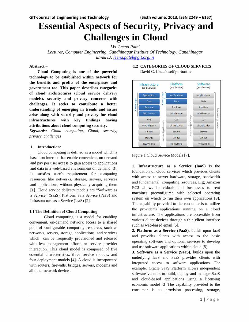
GIT-Journal of Engineering and Technology (Sixth volume, 2013, ISSN 2249 – 6157)
1 | P a g e
Abstract –
Cloud Computing is one of the powerful
technology to be established within network for
the benefits and profits of the enterprises and
government too. This paper describes categories
of cloud architectures (cloud service delivery
models), security and privacy concerns with
challenges. It seeks to contribute a better
understanding of emerging in trends and issues
arise along with security and privacy for cloud
infrastructures with key findings having
attributions about cloud computing security.
Keywords: Cloud computing, Cloud, security,
privacy, challenges
1. Introduction:
Cloud computing is defined as a model which is
based on internet that enable convenient, on demand
and pay per user access to gain access to applications
and data in a web-based environment on demand [3].
It satisfies user’s requirement for computing
resources like networks, storage, servers, services
and applications, without physically acquiring them
[1]. Cloud service delivery models are ―Software as
a Service‖ (SaaS), Platform as a Service (PaaS) and
Infrastructure as a Service (IaaS) [2].
1.1 The Definition of Cloud Computing
Cloud computing is a model for enabling
convenient, on-demand network access to a shared
pool of configurable computing resources such as
networks, servers, storage, applications, and services
which can be frequently provisioned and released
with less management efforts or service provider
interaction. This cloud model is composed of five
essential characteristics, three service models, and
four deployment models [4]. A cloud is incorporated
with routers, firewalls, bridges, servers, modems and
all other network devices.
1.2 CATEGORIES OF CLOUD SERVICES
David C. Chau’s self portrait is-
Figure.1 Cloud Service Models [7].
1. Infrastructure as a Service (IaaS) is the
foundation of cloud services which provides clients
with access to server hardware, storage, bandwidth
and fundamental computing resources. E.g; Amazon
EC2 allows individuals and businesses to rent
machines preconfigured with selected operating
system on which to run their own applications [3].
The capability provided to the consumer is to utilize
the provider’s applications running on a cloud
infrastructure. The applications are accessible from
various client devices through a thin client interface
such as web-based email [5].
2. Platform as a Service (PaaS), builds upon IaaS
and provides clients with access to the basic
operating software and optional services to develop
and use software applications within cloud [5].
3. Software as a Service (SaaS), builds upon the
underlying IaaS and PaaS provides clients with
integrated access to software applications. For
example, Oracle SaaS Platform allows independent
software vendors to build, deploy and manage SaaS
and cloud-based applications using a licensing
economic model [3].The capability provided to the
consumer is to provision processing, storage,
Essential Aspects of Security, Privacy and
Challenges in Cloud Ms. Leena Patel
Lecturer, Computer Engineering, Gandhinagar Institute Of Technology, Gandhinagar
Email ID: [email protected]

GIT-Journal of Engineering and Technology (Sixth volume, 2013, ISSN 2249 – 6157)
2 | P a g e
networks and other fundamental computing resources
where the consumer is able to deploy and run
arbitrary software, which can include operating
systems and applications [5].
1.3 TYPES OF CLOUDS
Figure.2 Public, Private and Hybrid Cloud
Deployment Example [11].
1. Private cloud- The cloud infrastructure is
operated for a specific organization. It may
be managed by the organization or a third
party and may be in house [11].
2. Community cloud- The cloud infrastructure
is shared by several organizations and
supports a specific community that has
shared concerns to the mission, security
requirements, policy, and compliance
considerations [5].
3. Public cloud- The cloud infrastructure is
made available to the general public or large
industry group and is owned by an
organization selling cloud services [6].
4. Hybrid cloud- Hybrid cloud is a private
cloud linked to one or more external
cloud services, centrally managed,
provisioned as a single unit, and
circumscribed by a secure network [14]. It
provides virtual IT solutions through a mix of
both public and private clouds. Hybrid Cloud
provides more secure control of the data and
applications and allows various parties to access
information over the Internet [13].
2. Security
A number of the current applications of cloud
computing involve consumer services, including e-
mail, and social networks. The protection of personal
data and management of privacy issues may well
determine the success or failure of many cloud
services [5].
As an OECD (Organization for Economic
Cooperation and Development) paper has noted:
Companies that wish to provide Cloud services
globally must adopt leading-edge security and
auditing technologies and best-in-class practices. If
they fail to earn the trust of their customers by
adopting clear and transparent policies on how their
customers’ data will be used, stored, and protected,
governments will come under increasing pressure to
regulate privacy in the Cloud. And if government
policy is poorly designed, it could stymie the growth
of the Cloud and commercial Cloud services [8].
2.1 Securing information within a cloud
computing environment requires three levels of
security: a) Network security
b) Host security
c) Application security.
Encryption for the information security is not a
complete solution because data needs to be decrypted
in certain situations – so that computation can occur
and the usual data management functions of indexing
and sorting can be carried out. Thus although data in
transit and data at rest are effectively encrypted, the
need to decrypt, generally by the cloud service
provider, can be a security concern. Nevertheless
cloud services can be augmented by email filtering
(including back-up, and spam), Web content filtering,
and vulnerability management, all of which improve
security [5].
2.2. SECURITY ON DEMAND
The Cloud Computing systems are secured
if users can depend on them (i.e. DaaS, SaaS,
PaaS,IaaS, and so on) to behave as users expect.
Traditionally, it contains 5 goals, say availability,
confidentiality, data integrity, control and audit, to
achieve adequate security. They are integrated
systematically, and none of them could be forfeited to
achieve the adequate security [16].

GIT-Journal of Engineering and Technology (Sixth volume, 2013, ISSN 2249 – 6157)
3 | P a g e
A. Availability
The goal of availability for Cloud Computing
systems is to ensure its users can use them at any
time, at any place [16].
B. Confidentiality
Confidentiality means keeping users’ data secret in
the Cloud systems. The confidentiality in Cloud
systems is a big obstacle for users to step into it, as
many users said ‖My sensitive corporate data will
never be in the Cloud‖ in the article named ‖Above
the Cloud‖ [16].
C. Data Integrity
Data integrity in the Cloud system means to preserve
information integrity (i.e., not lost or modified by
unauthorized users). As data is the base for providing
Cloud Computing services, keeping data integrity is a
fundamental task [16].
3. Privacy
Email, Instant messaging, business
softwares and web content management are
applications of the cloud environment. Many of them
have been used remotely through internet. E.g.
Microsoft recognizes privacy policies and protections
to obtain trust of customers. Even secured systems
and datacenters help to protect privacy and support
[9].
3.1 Privacy Questions in Cloud Computing
Are hosted data and applications within the cloud
protected by suitably robust privacy policies?
Are the cloud computing provider’s technical
infrastructure, applications, and processes secure?
Are processes in place to support appropriate
action in the event of an incident that affects privacy
or security?
Security is an essential component of strong privacy
safeguards in all online computing environments, but
security alone is not sufficient. Consumers and
businesses are willing to use online computing only if
they trust that their data will remain private and
secure [9].
4. Legal and Regulatory Challenges
Cloud services can thrive when companies are
able to provide cloud services in an efficient way and
assure customers that their data will remain private
and secure [9].
4.1 Challenges
The following are some of the notable
challenges associated with cloud computing, some of
them lead to the delay in services and some give the
opportunity to be resolved with due care and focus
[10] :
• Security and Privacy —these challenges can be
addressed, for example, by storing the information
internal to the organization, but allowing it to be used
in the cloud. For this to occur, though, the security
mechanisms between organization and the cloud need
to be robust and a Hybrid cloud could support such a
deployment [10].
• Lack of Standards — Clouds have documented
interfaces; however, no standards are associated with
these, and thus it is unlikely that most clouds will be
interoperable. The Open Grid Forum is developing an
Open Cloud Computing Interface to resolve this issue
and the Open Cloud Consortium is working on cloud
computing standards and practices. The findings of
these groups will need to mature, but it is not known
whether they will address the needs of the people
deploying the services [10].
• Continuously Evolving — User requirements are
continuously evolving, as are the requirements for
interfaces, networking, and storage. This means that a
―cloud,‖ especially a public one, does not remain
static and is also continuously evolving [10].
• Compliance Concerns —these challenges typically
result in Hybrid cloud deployment with one cloud
storing the data internal to the organization [10].
5. Key Findings with Attributions about cloud
computing security
Bar Chart 1 reports cloud providers’
agreement with three attributions about cloud
computing security. These findings indicate that
respondents overwhelmingly believe it is the
responsibility of users of cloud computing to ensure
the security of cloud resources they provide. The
majority does not believe their cloud services include
the protection of sensitive data. Further, only 19
percent of US cloud providers and 18 percent of
European cloud providers strongly agree or agree that
their organization perceives security as a competitive
advantage in the cloud marketplace [2].

GIT-Journal of Engineering and Technology (Sixth volume, 2013, ISSN 2249 – 6157)
4 | P a g e
Bar Chart 1: Cloud providers’ attributions about
cloud computing security [2].
As shown below in Bar Chart 2, the majority of cloud
providers (79 percent) say their organizations allocate
10 percent or less of IT resources or efforts to
security and control-related activities [2].
Bar Chart 2: Percent of resources dedicated to
security and control-related activities [2].
US & Europe results combined
As shown in Bar Chart 5, when asked why
companies purchase cloud computing services, the
top choices are reduced cost, faster deployment time,
improved customer service and increased efficiency.
The least cited reasons are improved security and
compliance with contractual agreements or policies
[2].
Bar Chart 3: Reasons customers migrate to the cloud
computing environment [2].
US & Europe results combined
This concludes that the focus on cost and speed and
not on security or data protection creates a security
hole. This may explain why 62 percent of US and 63
percent of European providers are not confident or
unsure that cloud applications are sufficiently
secured. As noted in Bar Chart 4, two thirds of US
cloud providers and 61 percent of European cloud
providers are not confident or are unsure that their
customer’s security requirements are met. Similarly,
there is a lack of confidence that their cloud
applications and other resources are secure [2].
Bar Chart 4: Lack of confidence in the security of
cloud resources provided [2]. Not confident & unsure
response combined
Bar Chart 5 provides responses to two separate but
related questions about the provisioning of IT
security services as a possible product offering. Most
cloud providers (91 percent) do not provide security
as a service from the cloud today, but about one-third
are considering offering this type of service at some
point in the next two years [2].
Bar Chart 5: Security as a service from the cloud
5. Conclusion

GIT-Journal of Engineering and Technology (Sixth volume, 2013, ISSN 2249 – 6157)
5 | P a g e
The study of research determines the aspects
and dimensions for establishing security and
privacy with challenges which would be
leading-edge to more efficient and secured
cloud services in the cloud infrastructures.
By using a cloud system, your company’s
sensitive data and information will be stored
on third-party servers. This article will be
helpful to establish a future’s powerful and
efficient plus secured network through
internet using cloud services. It will be the
advanced new technology to the new era and
future enhancement. This paper will lead IT
professionals to conduct high quality,
empirical studies on critical issues affecting
the management and security of sensitive
information about people and organizations.
References
[1] Choubey, 2011. A survey on cloud
computing security, challenges and threats.
Bhopal, India: IJCSE.
[2] Security of Cloud Computing Providers
study. Ponemon Institute, Researched report.
Sponsered by CA Technologies.April, 2011.
[3] Kim-Kwang Raymond Choo, (2010). Cloud
computing: Challenges and future
directions. Australian Government,.
Australian Institute of Criminology (Trends
and Issues in crime and criminal justice).
Page No.400.
[4] National Institute of Standards and
Technology, December 2009, Guidelines on
security and privacy in public cloud
comuting. [online]. US, special publication
800-144, US department of commerce.
Standard from Information Technology
Laboratory (NIST), accessed on
14 May 2012 at
http://csrc.nist.gov/groups/SNS/cloud-
computing/cloud-def-v15.doc
[5] Mudge, J C. (2010). CLOUD
COMPUTING: Opportunities and
Challenges for Australia.[online] Executive
summery by The australian academy of
Technological sciences and engineering
(ATSE). Last accessed on 15 May 2012 at
http://www.egov.vic.gov.au/trends-and
issues/information-and-communications
technology/cloud-computing/cloud-
computing-opportunities-and-challenges-
for-australia-in-pdf-format-1367kb.html
[6] Wyld, D C, (2010). The cloudy future of
government IT: Cloud computing and the
public sector around the world. [online]
International Journal of Web & Semantic
Technology (IJWesT), Vol 1, Num 1,
January 2010, Last accessed on 22 June
2010 at
http://airccse.org/journal/ijwest/papers/0101
w1.pdf
[7] Chou D C, 16th
August 2010. Figure-1, self
portrait. [Online image]. Last accessed at 9th
May, 2012 at:
http://blogs.msdn.com/b/johnalioto/archive/
2010/08/16/10050822.aspx
[8] Nelson M R, (2009). Organization for
Economic Cooperation and Development.
Briefing paper for the ICCP Technology
Foresight Forum: Cloud computing and
public policy, Last accessed on 22 June 2010
at
http://www.oecd.org/dataoecd/39/47/439337
71.pdf
[9] Microsoft. (2009). Privacy in the Cloud
Computing Era; A Microsoft Perspective,
page.no.9 [online]. Lasr accessed on 16 May
2012 at
http://download.microsoft.com/download/3/
9/1/3912e37e-5d7a-4775-b677-
b7c2baf10807/cloud_privacy_wp_102809.p
df
[10] Dialogic Corporation, (2010). White Paper:
Introduction to cloud computing. [Online].
Last accessed on 14 May 2012 at
www.dialogic.com.

GIT-Journal of Engineering and Technology (Sixth volume, 2013, ISSN 2249 – 6157)
6 | P a g e
[11] Machi J., 2010. Figure-2., Dialogoc
Exchange Network, Corporate Blog [online
image]. Last accessed on May 15, 2012 at
http://blog.tmcnet.com/industry-insight/
[12] Department for Culture, Media and Sport
(DCMS) and Department for Business,
Innovation and Skills (DBIS), 2009, Digital
Britain: Final Report, London.
[13] Kuyoro S. O., Ibikunle F. & Awodele O.,
2011. Cloud Computing Security Issues and
Challenges International Journal of
Computer Networks (IJCN), Volume (3) :
Issue (5) : 2011,p249.
[14] Global Netoptex corporated.―Demystifying
the cloud. Important opportunities, crucial
choices.‖ pp4-14[online].Last accessed on
May 15,2012 at:
http://www.gni.com
[15] Minqi Zhou,Rong Zhang, Wei Xie, Weining
Qian, Aoying Zhou, (2010). Security and
Privacy in Cloud Computing [online]. In:
Sixth International Conference on
Semantics, Knowledge and Grids. Software
Engineering Institute, East China Normal
University, Shanghai 200062, p106. Last
accessed on May 16, 2012 at
mqzhou,wxie,wnqian,[email protected]
du.cn, [email protected].
[16] M. Armbrust, A. Fox, R. Griffith, A.
Joseph, R. Katz, A. Konwinski, G. Lee, D.
Patterson et al., ―Above the clouds: A
Berkeley view of cloud computing,‖
University of California, Berkeley,Tech.
Rep, 2009.

GIT-Journal of Engineering and Technology (Sixth volume, 2013, ISSN 2249 – 6157)
System Description Formation for University
Blackboard Tool
Birendrasinh.K.Zala, Gandhinagar Institute of Technology, Gandhinagar
Abstract: A major challenge, and thus opportunity, in the field of
usability engineering is developing effective system description
for system which has no fixed guidelines. I present an exemplar
system description report on University Blackboard Tool which
is developed to establish effective channel of communication and
collaboration to next phases of usability engineering are called
system redesign and system evaluation. This paper will discuss all
steps of system description for University Blackboard in a very
general manner. The research method used is Formative
Evaluation.
Index terms: User Centered System Design (UCSD), Human
Computer Interaction (HCI), Information and Communication
Technology (ICT).
Keywords: Formative Evaluation, Mapping, System Domain,
Usability, Task Characteristics.
I INTRODUCTION
HCI focus on verifying three main things like system is self
learnable for users [1], complexity of interaction and filling
the gap between the system image and user’ model. To get
success in all three factors we don’t need to look around we
already have one approach called User Centred System Design
(UCSD) [2]. Domain area for this study includes University
Blackboard Tool which specifies target system for users
SYSTEM DOMAIN
Organizing and facilitating group work can be a daunting
experience for students. They may be paired with students
who have quite different timetables and work/study
arrangements. Finding time to schedule meetings and effective
methods of collaborating on work can be very frustrating. One
thing all the students have in common is Blackboard.
Blackboard has a number of features which try to support
group work and organization independently. Firstly, there is
the Group Area where tutors can create a private area for each
group of students to carry out their own discussions and post
files. Secondly, there are the calendar and task tools. Students
can add events and tasks to their own Blackboard calendars. In
addition, lecturers can also add tasks for all students in their
unit. The aim of this project is to develop an add-on for
Blackboard (known as a Building Block) that will help
students manage the process of group work. UCSD approach
includes System Description phase which gather, identifies
and specifies all basic requirements to produce a base for
system redesign phase.
This paper discusses steps which performed during the system
description formation of University Blackboard Tool. Formative Evaluation (both formal and informal) is an
observational, empirical evaluation method that assesses user
interaction by iteratively placing representative users in task-
based scenarios in order to identify usability problems, as well
as to assess the design’s ability to support user exploration,
learning, and task performance[3].
II CASE STUDY: A USER-BASED STUDY EXAMINING
UNIVERSITY BLACKBOARD TOOL
One of the three phases of usability engineering will be
explained in this part of paper with respect to one example
system which is a Blackboard tool for a university they are
developing for the faculty members and students.
SYSTEM DESCRIPTION
The Group Work Tool (Blackboard Add-on) shall support
students, lectures and tutors for academic purposes where
group[4] or team work is involved. This is a type of
groupware tailored suit the existing academic environment.
Blackboard tool relies on the Internet. Also group related data
can only be accessed by relevant group members. However, in
some subjects the convener or tutor needs to assess each group
member’s contribution by viewing the group area. Assigned

GIT-Journal of Engineering and Technology (Sixth volume, 2013, ISSN 2249 – 6157)
staff members for the subject should be able to carry out this
assessment as well.
This groupware should be able to provide non-collocated users
to interact in synchronous or asynchronous manner. This
product has to cater groups of varied interaction styles as
group composition changes from one to another and it changes
from assessment item to another. Therefore different
communication mechanisms need to be present in this tool.
Share messages among members, replying messages.
Email facilities
Instant messaging.
Moreover product shall support sharing documents via a
central repository of documents and versioning of progressive
documents. This product shall support setting appointments,
managing events and calendar capabilities to setup meeting
times so that students can perform their task in a timely and
informed manner. In addition it allows task allocation for
individual students so that group as a whole knows what the
responsibilities of each student students
CONCEPT MAPPING
The blackboard building block is tool, useful for the student in
their course of study where he/she can store the files;
communicate with the staff, student and the group mates. They
can access the assessment, view the message board, messaging
and email with this tool. The calendar that enables students to
add events setup reminders on specific dates.
Figure.1. Concept mapping Design for Blackboard tool.
USER DESCRIPTION
The primary users[4] if this system will be students. And
Lecturers and tutors can be considered secondary users as they
may use this product less frequently than students.
Table 1. User Profile: Student (primary user)
Attribute User Characteristics
Age 18 – 35
Gender Male (60%)/female (40%)
Physical
abilities and
disabilities:
Probably have small number of less-able
students
Vision – average - good (May have students
with low level.)
Hearing –good
Educational
Background
Secondary (25%), Bachelors(55%)/ Masters
(20%)/
Computing
and IT
experience
Novice/Intermediate/Experienced
( Novice:0 to 3 months
Intermediate : more than three months, less
than one year
Experience :more than one year)
Basic Computer skills
Generally good.
Able to use office software.
But new students may find it difficult at the
beginning.
ICT students tend to be more comfortable.
Experience with blackboard/ blackboard
Group area After few weeks into the studies at
university, students can become
comfortable.
Experience with other groupware tools
(e.g. Outlook Express, Lotus Notes)
Novice, Intermediate
Less likely to use full featured collaborative
software.
Motivation
High (eg. they find it difficult to manage
group assessments. Help of a tool is
appreciated, some motivated by group
environment)
Moderate
Low: some may not even like the idea of
group work due to bad experiences.
Attitude
Positive (80%): As enabling tools for
studies. Use of similar tools makes them
comfortable.

GIT-Journal of Engineering and Technology (Sixth volume, 2013, ISSN 2249 – 6157)
Quick learning ability. Can do attitude.
May have confidence (20%): Impression of
hard to learn may not like group work at all.
USER GOALS
1. Lecturer
Form a group of students.
Communicate the student about updates of
the assignment.
2. Student
Share a file with group members.
Send a message to the group members
Reply to a message sent by a group member.
TASK CHARACTESTICS
Following are goals are represented as a sequence of tasks and
the characteristics tasks involved.
Form a group of students.
1. Lecturer selects to create a group.
2. Select a student to join the group.
3. Add this student to the group.
4. Add more students to the group until desired number
of students per group are reached.
ANALYSIS OF CURRENT SYSTEM
According to our system domain primary user, Student had
goals like according to previous analysis; Communication
with students who are in the same group is one of the goals.
Based on interviews conducted, we were able to find out the
following problems. Interviews/observations were targeted on
group activities
1. Reluctance to use group area emailing facility.
Instead they use Web mail (Through
Blackboard/directly) Reasons as per users
Does not look appealing.
More used to web mail as they use it more
often.
2. Lack of integration When using web mail for communication with group
members lack integration between backboard and
web mail causes inconvenience. Instant switching
from blackboard to web mail requires login with
different credentials.
3. Security.
In addition web mail credentials cannot be changed.
It stays as student Id (username) and date of birth.
As students use web a mail for group work we will discuss the
issues of web mail in relation to ―Lack of integration and
security‖.
USASBILITY METRICS
Developers using Usability metrics to identified the problems
in the system domain before the system releases.
Efficiency
Time to learn on a specified task.
Time to complete a specified task
Time spent on errors
Number of bugs
Based on the observations
Time to learn on a specified task.
User had good experience before using the web mail,
like hotmail, MsOutlook. Not difficult to learn.
Time to complete a specified task
In relation to the selected goal, based on our
observation, real user would have thought few steps
to be unnecessary. Login twice, address book tasks.
Completed fairly quickly took around (40-50s it was
a short message)
Time spent on errors
The user had fairly good knowledge of the domain
and knew how to fulfill the goal using web mail.
Number of bugs
During the observation did not come across any
bugs/errors
Effectiveness
Number of tasks completed (percentage)
Workload of the specified tasks
Ratio of success to failure
Based on the observations
Number of tasks completed
Completed around 7 for the selected goal, but user
feels that can be reduces
Workload of the specified tasks
User felt it was a simple set of tasks, but can refine it
more
Ratio of success to failure
Did not fail to complete the task
Satisfaction
Rating scale of the usefulness of system domain
Rating scale of the satisfaction of features
Number of times real users express frustration and
less satisfaction
Based on the observations
On a scale of 1-5
Rating scale of the usefulness of system domain: 4
Rating scale of the satisfaction of features: 3
Number of times real users express frustration and
less satisfaction: 2

GIT-Journal of Engineering and Technology (Sixth volume, 2013, ISSN 2249 – 6157)
III CONCLUSION
At the end of system analysis some of the problems uncovered
like Student feel lack of integration between two systems
(blackboard and web mail). They find it inconvenient to login
to web mail, switch back to blackboard to do some work and
again to mail and so on even though it is link to blackboard.
And Users can’t change their default password which is a
concern for the students. Security wise they have concerns. System description phase provides input to the next phase
called system design report to help developers implement
system better.
IV REFERENCES
[1] C. Abras, D. Maloney-Krichmar, and J. Preece, ―User-Centered
Design,‖ In W. Bainbridge (Ed.), Encyclopedia of Human-Computer
Interaction, Thousand Oaks, Sage Publications, 2004.
[2] J. Gulliksen, B. Goransson, I. Boivie, S. Blomkvist, J. Persson,
and A. Cajander, ‖Key principles for user-centred systems design,”
Behaviour and Information Technology, 22(6), 2003, pp. 397-409.
[3] S. Sade, M. Nieminen, and S. Riihiaho,‖ Testing usability with
3D paper prototypes—Case Halton system,‖ Applied Ergonomics,
29 (1), 1998, pp. 67-73.
[4] C. Courage and K. Baxter,‖ Understanding your users: A
practical guide to user requirements, methods, tools and techniques,‖
2005, pp. 25.
[5] D. Bowman, J. Gabbard, and D. Hix, ―A Survey of Usability
Evaluation in Virtual Environments: Classification and Comparison
of Methods,‖ Presence: Teleoperators and Virtual Environments,
vol. 11, no. 4, 2002, pp. 404-424

GIT-Journal of Engineering and Technology (Sixth volume, 2013, ISSN 2249 – 6157)
Abstract—With the Internet usage gaining fame and the stable
growth of users, the World Wide Web has become a huge
repository of data. The increasing volume of information on the
Web is the main motivation for recommender systems: they
support users while they interact with large information spaces,
directing them toward the information they need.
Social tagging is an innovative and powerful mechanism
introduced with Web 2.0: it shifts the task of classifying resources
from a reduced set of knowledge engineers to the wide set of Web
users.
This paper is a survey which discusses the role of tags in
recommender systems. The aim of this paper is to analyze the
state of the art related to the role of tags in social tagging systems,
specifying how tags are actually used by users, how recommender
systems use tags for suggesting resources and how the process of
tagging is supported by tag recommendations.
Index Terms— Tag, social tagging, recommender system,
personalization, Web 2.0.
I. INTRODUCTION
Each day, the Internet grows by roughly a million electronic
pages, adding to the hundreds of millions pages already on-
line. As a result, Web users are always drowning in an “ocean”
of information and facing the problem of information overload
when interacting with the web. Because of speedy growth of
the information, the resulting arrangement of information lacks
of organization and structure. Users often feel confused and
get lost in that information overload that continues to expand.
Therefore, the crucial need nowadays is that of predicting the
user needs in order to improve the usability and user retention
of a web site. It is necessary for a Web developer or designer
to know what the user really wants to do, predict which pages
the user is potentially interested in, and present the customized
Web pages to the user [2].
Web personalization is a strategy, a marketing tool, and an
art [2]. The objective of a Web personalization system is to
“provide users with the information they want or need, without
expecting from them to ask for it explicitly” [3].
Web 2.0 applications are based on a set of technologies
which provide users with tools for creating, sharing and
promoting new content: users can easily leave the role of
passive consumers of resources and become active producers
of information. This trend increases both the knowledge on the
Web and the number of available resources. Actually, the
growing number of resources prevents an effective access to
knowledge: a user needs to read the content of resources for
evaluating if it is what she really wants to know. An effective
classification of the resources can improve the access to
knowledge.
Social tagging applications [4] allow users to freely
associate labels (known as tags) to resources, distributing the
task of classifying document over the set of Web 2.0 users.
Social tagging systems do not require significant efforts:
human classifiers do not have to follow specific rules and may
classify only the set of resources they consider interesting.
Social tagging applications have both private and public
aspects [4]:
• Users apply tags for personal aims: typically they
associate labels to resources in order to find them again.
• Each user can enjoy the classification applied by other
users. A user can browse available documents following
classifications provided by other users.
However, due to the freedom of social tagging systems the
classification process is not precise. This means that the
classification applied by a user may be not useful to other
users. In order to improve the access to resource classified in
social tagging systems we needs of technologies able to
overcome this limitation adapting the available classification
to the specific user [1].
Recommender systems have been proposed for supporting
users in social tagging system to sort resources which appear
related to target users according to their interests and their
tagging habits.
The aim of this paper is to analyze the state of the art related
to the role of tags in social tagging systems, specifying how
tags are actually used by users, how recommender systems use
tags for suggesting resources and how the process of tagging is
supported by tag recommendations.
The rest of this paper is organized as follows: Section II
introduces social tagging and recommender systems; Section
III deepens the discussion on the use of tags for recommending
content, while Section IV illustrates the use of tags for
recommending tags. Final considerations and a look to the
future close the paper.
A SURVEY ON RECOMMENDING TAGS
METHODOLOGIES
Prof. Brinda Parekh

GIT-Journal of Engineering and Technology (Sixth volume, 2013, ISSN 2249 – 6157)
II. BACKGROUND
In this section we present an overview of social tagging and
recommender systems, describing in particular how tags are
applied by users, what are limitations connected to the tagging
process, and how the recommender systems.
A. Social tagging systems
Social tagging is an innovative and powerful mechanism
introduced with Web 2.0: it shifts the task of classifying
resources from a reduced set of knowledge engineers to the
wide set of Web users.
A tag is a term freely chosen by a user as significant for a
resource; it represents a metadata describing the item, so it can
be useful as a keyword to identify or to find again later a
document. Tags are also the main mechanism used to browse
and search new resources in social tagging systems.
The collection of all the tag assignments performed by a
user constitutes her personomy, while the collection of all
personomies constitutes a folksonomy.
Nevertheless, tags contain very useful, social/semantic
information, and their nature can be better understood by
analyzing the various motivations/goals that lead a user to
perform tagging [5,6,7].
Common purposes are [1]:
Describe the content. Tags may be used for summarizing
the content of the resource.
Describe the type of the document. Some users use tags
for identifying the kind of document. A document may
be classified according to its MIME type (for example
pdf, doc) or taking into account the publication form
(article, blog, book).
Describe features and qualities. Adjectives (such as
’interesting’, ’good’, and so on) may be used for
expressing opinions, emotions or qualitative judges.
Associate people to documents. Tags can report the
authors of a document or people involved in a
particular task or event. Moreover, tags such as ’my’,
’mycomments’, ’mystuff’, and so on are used to define
a relationship between the resources and the tagger.
Associate events to documents. Locations, dates,
conferences acronyms are widely used for associating
an event to a document.
Associate tasks to documents. Some tags, such as
’mypaper’, ’to read’, ’jobsearch’ reveal personal
matters or engagements.
These possible motivations should be considered together
with the following two further factors:
1. Heterogeneity of users. Taggers have different levels
of expertise and goals. This has several consequences:
classifications exploited by some users may be not
understandable (or acceptable) for other users; different users
may describe the content of a resource using distinct
vocabularies; different users may have different opinions about
a topic; users may not have knowledge about people, events or
tasks associated to a resource by other users.
2. Temporal changes. Users’ knowledge, motivations, and
opinions may change over the time. A tag used today for
describing an item can be useless in the future: emotions and
opinions of people may change; reputation of people evolves;
a topic may be not any more interesting to the user.
B. Recommender systems The increasing volume of information on the Web is the
main motivation for recommender systems: they support users
while they interact with large information spaces, directing
them toward the information they need [8]; these systems
model user interests, goals, knowledge and tastes, monitoring
and modeling some implicit and/or explicit feedback. User
feedback can be acquired by means of ratings for quantifying a
relation between the user and an item: the ratings may be
explicit, when they require the user evaluation, or implicit
when they are automatically generated by the system in terms
of measures, such as, for example, the time spent by a user on
a Web page. By taking in consideration the ratings provided
by a user, a recommender system defines a personalized order
of importance for the set of available resources.
According to the strategy used for collecting and evaluating
ratings, recommender system can be classified into three main
classes [1]:
1. Collaborative filtering recommender systems.
Collaborative filtering recommender systems [9] implement
the idea that a user, that shares interests, knowledge and goals
with a community, with good probability may be interested in
the documents which appear relevant to that community. For
this reason, a collaborative filtering recommender system
builds and maintains a profile for each user and computes
similarities among users: similar users, known as neighbors,
are the bridge which allows the user to receive suggestions for
new potentially interesting content. In turn, collaborative
filtering approaches can be classified into two classes [10]:
• Model-based approaches, which build a probabilistic
model for predicting, on the basis of user history, her future
rating assignments.
• Memory-based approaches, which use statistical
techniques for identifying users with common behaviour.
When the neighborhood has been defined,
neighbors’feedbacks are combined for generating a list of
recommendations.
2. Content-based recommender systems. Contentbased
recommender systems [11] analyze the past user activities
looking for resources she liked; they model resources
extracting some features from documents. The user profile is
then defined describing what features are interesting for the
user. The relevance of a new resource for a user is calculated
matching the representation of the resource to the user profile.
3. Hybrid recommender systems. The results returned by
collaborative and content-based recommender systems can be
combined in a hybrid recommender system [12], applying
several different strategies:
• A weighted hybrid recommender system merges results of
different techniques. The score of an item is defined as a

GIT-Journal of Engineering and Technology (Sixth volume, 2013, ISSN 2249 – 6157)
weighted sum of scores calculated by different recommender
systems.
• A cascade hybrid recommender system filters a starting set
of resources using a first recommender system. The ranking of
these resources is then refined by a second recommender
system.
• A switching hybrid recommender system uses one of the
available recommender system according to some criterion.
• A feature combination hybrid recommender system
considers collaborative data as the features used in content-
based approaches.
III. RECOMMENDING TAGS
Recommender systems can suggest to the user not only
content, by also tags for labeling for a resource: this typology
of recommendation aims to improve the usage of social
tagging applications [13]:
Tag suggestions can increase the probability of having
tagged resources. Users just select one or more
suggested tags instead of summarizing a resource in
order to find representative tags.
Tag suggestions can promote a common vocabulary
among users. Proposing a well defined set of tags it is
possible to reduce problems connected to the absence
of both guidelines and supervised methodologies to
the tagging process.
The methodologies can be classified by means of three
classes [14]:
• Content-based tag recommender systems. These systems
look to the content of resources for suggesting relevant terms
to the user.
• Collaborative tag recommender systems. Collaborative
approaches analyze metadata associated by users to resources
inferring the relevance of tags for the specific resource.
• Graph based tag recommender systems. These systems
build a graph representation of a folksonomy which can be
explored for finding tags to be recommended.
Different tag recommender systems use different criteria for
evaluating the relevance of tags to be suggested. According to
the relevance criteria tag recommender systems can be divided
into two classes:
1. Not personalized tag recommender systems. These
systems select for each document the best tags to describe the
specific resource, ignoring user’s tagging habits. Different
users will receive the same suggestions for the same resource.
2. Personalized tag recommender systems. These systems
suggest the set of the most relevant tags for a resource
according to the specific user and her personal way to classify
resources.
IV. FINAL CONSIDERATIONS
In this paper we described some important limitations of
current social tagging systems, discussing the different
methodologies applied by recommender systems for improving
the access and the classification of resources. Summarizing,
collaborative approaches model the user’s tagging behavior
and look for users with similar tagging habits: these systems
are based on the idea that users with similar interests search
and bookmark similar resources. On the other hand, content-
based approaches use tags to build a user profile and then
suggest resources which appear relevant for the specific user
profile. Both collaborative and content approaches have
limitations mainly due to ambiguity of tags.
REFERENCES
[1] Antonina Dattolo, Felice Ferrara, Carlo Tasso," The role of tags for recommendation: a survey”, Rzeszow, Poland, May 13-15, 2010.
[2] A.Jebaraj Ratnakumar ,“An Implementation of Web Personalization
Using Web Mining Techniques”. Journal of Theoretical and Applied
Information Technology. Page 1, 2005.
[3] Brinda R. Parekh, Pooja Mehta, Prof. Kirit J. Modi, Prof. Paresh S.
Solanki, “Web Personalization Using Web mining: Concept &
Research Issues”, International Journal of Information and Education
Technology, Mumbai, 2012.
[4] Mathes, A.: Folksonomies cooperative classification and communication
through shared metadata. computer mediated communication -
lis590cmc. http://www.adammathes.com/academic/ computer-
mediatedcommunication/folksonomies.html (2004)
[5] Golder, S., Huberman, A.: The structure of collaborative tagging
systems. Journal of Information Science 32(2) (2006)198-208.
[6] Dattolo, A., Tomasi, F., Vitali, F. In: Towards disambiguating social
tagging systems. Volume 1, Chapter 20. IGI-Global (2010) 349–369.
[7] Xu, Z., Fu, Y., Mao, J., Su, D.: Towards the semantic web:
Collaborative tag suggestions. In: Proceedings of the Collaborative Web
Tagging Workshop at the World Wide Web Conference. (2006).
[8] Adomavicius, G., Tuzhilin, A.: Toward the next generation of
recommender systems: A survey of the state-of-the-art and possible
extensions. IEEE Transaction on Knowledge andData Engeneering
17(6) (2005) 734–749.
[9] Schafer, J., Frankowski, D., Herlocker, J., Sen, S.: Collaborative
filtering recommender systems. In Brusilovsky, P., Kobsa, A.,
Nejdl,W., eds.: The AdaptiveWeb. LNCS (4321).Springer-
Verlag, Berlin, Germany (May 2007) 291–324
[10] Breese, J., Heckerman, D., Kadie, C.: Empirical analysis of
predictive algorithms for collaborative filtering. In: Proceeding
of the Fourteenth Conference on Uncertainty in Artificial Intelligence (UAI), Morgan Kaufmann (1998) 43–52.
[11] Pazzani, M.J., Billsus, D.: Content-based recommendation
systems. In Brusilovsky, P., Kobsa, A., Nejdl, W., eds.: The
Adaptive Web. LNCS (4321). Springer-Verlag, Berlin,
Germany(May 2007) 325–341
[12] Burke, R.: Hybrid web recommender systems. In Brusilovsky,
P., Kobsa, A., Nejdl, W., eds.: The Adaptive Web. LNCS
(4321). Springer-Verlag, Berlin, Germany (May 2007) 377–408
[13] J¨aschke, R., Marinho, L., Hotho, A., Schmidt-Thieme, L.,
Stumme, G.: Tag recommendations in social bookmarking
systems. AI Commununications 21(4) (2008) 231–247
[14] Musto, C., Narducci, F., De Gemmis, M., Lops, P., Semeraro,
G.: Star : a social tag recommender system. In: Proceedings of
the ECML/PKDD 2009 Discovery Challenge Workshop.(2009)

GIT-Journal of Engineering and Technology (Sixth volume, 2013, ISSN 2249 – 6157)
Study and Review of Various Identity and Privacy
Management Techniques in Consumer Cloud Computing Archana N. Mahajan
#, Sandip S. Patil
*
#Research Scholar, Computer Engg Department
, S.S.B.T.’s College of Engg.& Tech.,
North Maharashtra University Bambhori,Jalgaon(M.S.) [email protected]
* Associate Professor in Computer Engg Department
S.S.B.T.’s College of Engg. and Technology Bambhori, Jalgaon(M.S.) 2 [email protected]
Abstract— Consumer cloud computing is the result of expected
evolution and integration of advances in several areas such as
distributed computing, service oriented architecture, and last but
not the least consumer electronics. We can say that integration of
consumer electronics that is home networks with cloud
computing is known as consumer cloud computing. In this paper
we are presenting abstractive study of identity and privacy
management in consumer cloud computing. In the consumer
cloud environment, all attention and energy is given to
distribution of information and heterogeneity of clouds but less
attention is given to security and identity management challenges
in this context.
Keywords— Consumer cloud computing, Identity Management,
SAMLv2, dynamic federation establishment,Privacy.
I. INTRODUCTION
Cloud computing is a large scale distributed computing
model in which computing resources are available to cloud
consumers via Internet. The key characteristics of the cloud
are the ability to scale and provision computing power
dynamically in a cost efficient way and the ability of the
consumer (end user, organization or IT staff) to make the most
of that power without having to manage the underlying
complexity of the technology. The cloud architecture itself
can be private (hosted within an organization’s firewall) or
public (hosted on the Internet). The consumer cloud
computing platform is a networked collection of servers,
storage systems, and devices in order to combine software,
data, and computing power scattered in multiple locations
across the network. Consumer cloud computing offers
resources as services that are more flexible, scalable,
affordable and attractive to customers and technology
investors. Thus consumer cloud computing enables different
applications related to consumer electronics (CE), such as
virtualization of consumer storage, CloudTV platforms that
provide access to a number of Web applications such as social
networking, user generated video games, etc[1].
II. IMPORTANCE OF IDENTITY MANAGEMENT IN
CONSUMER CLOUD ENVIRONMENT
Service providers use infrastructure provided by Cloud
Computing provider to provide their services to their
customers. While using these services, consumers provide the
service providers with sensitive data such as civil ID (name),
SSN number, credit card information in order to have access
to these online services. Current privacy laws require cloud
computing service providers to implement varied security
measures depending on the nature of the information.
However, consumers can not verify that a provider of a
service conform to the privacy laws and protect their digital
identity. Given this, a consumer has to decide as what type of
personal information they could provide.
For example, a “Twitter breach of information stored on
Google Apps” shows the implications of leakage of private
information in cloud security. The July 15 disclosure by
Twitter exposed that a hacker had accessed a substantial
amount of company data stored on Google Apps. First the
hacker hijacked a Twitter employee's official e-mail account.
Then, he took advantage of poor password practices,
Hotmail's inactive account feature and personal information
on the Web to access hundreds of Twitter documents. This
probes the weakness of the username/password security token
used by most service providers to authenticate consumers,
which leaves the consumer susceptible to phishing attacks. [2]
Many organizations are uncomfortable with storing their data
and applications on systems they do not control. Migrating
workloads to a shared infrastructure increases the potential for
unauthorized exposure. Consistency around authentication,
identity management, compliance, and access technologies
will become increasingly important. To reassure their
customers, cloud providers must offer a high degree of
transparency into their operations.
A. Identity management and authentication in consumer
cloud computing
In the consumer cloud environment, all attention and energy
is given to distribution of information and heterogeneity of
clouds: private, community, public, and hybrid but less
attention is given to security and identity management
challenges in this context. For example, users in a private
cloud should be able to access applications hosted in a

GIT-Journal of Engineering and Technology (Sixth volume, 2013, ISSN 2249
– 6157) community cloud as long as a trust relationship exists between
cloud domains, which represents different forms of their
identities. This is due to cloud scenarios are multi-provider
and multi-service. Also applications in cloud computing may
combine data from multiple cloud-based sources, which hold
different conditions of service, privacy policies, and location.
Thus, because of the distributed and open nature of cloud
environments, it is necessary to dynamically propagate trust
for managing digital identity related to access control,
reputation, anonymity and privacy in different domains in a
protected and flawless manner.
For this purpose, federated Identity Management (IdM) has
developed. This helps for enabling global scalability which is
required for the successful implantation of cloud technologies.
Federated identities are based on the user-centric profiles,
which protect consumers from cloud computing services.
In the context of consumer electronics, federations of clouds
have right to alter how CE device applications are developed,
deployed or used while simultaneously removing constraints
on device functionality; into home private clouds, public
clouds, etc. For example, consider a consumer cloud scenario,
in which cloud federation allows Alok to build different layers
in his car navigation map to get recommendations for the best
routes (CSP1); as well as consult relevant information on sites
close to his position, in a Cloud Tourist Information Provider
(CSP2), by means of the cooperation between his mobile and
the car navigator. In addition, Alok can connect to his Social
Network (CSP3) to see if some friends have been on that site
and share information with them without compromising his
privacy [1]. However, federated IdM systems not have
mechanisms to achieve agile and dynamic federation, which is
one of the most significant architectural issues. Dynamic
federation requires allowing agile decision making without
requiring static pre-configuration. There are various standards
for federated IdM which include privacy considerations, but
they do not cover all aspects related to anonymity,
pseudonyms or tracking.
In addition, current IdM specifications support partial
anonymity, define poor privacy policies or they are complex
to implement. A similar situation can be found in the case of
audit mechanisms.
B. Existing identity management tools
Some known identity management tools are as follows: -
1. OpenID[May 2005]
The original OpenID authentication protocol was developed in
May 2005 by Brad Fitzpatrick, creator of popular community
website LiveJournal. Initially referred to as Yadis (an
acronym for "Yet another distributed identity system"), it was
named OpenID after the openid.net domain name was given to
use for the project. With OpenID a user uses one username
and one password to access many web applications. The user
authenticate to an OpenID server to get his/her OpenID and
use the token to authenticate to web applications. A user of
OpenID does not need to provide a service provider with his
credentials or other sensitive information such as an email
address. OpenID is a decentralized authentication protocol.
No central authority must approve or register service
providers or OpenID Providers. An end user can freely choose
which OpenID Provider (OP) (OpenID Authentication server
on which a service provider relies to assert the authenticity of
the identity of the consumer) to use, and can preserve their
Identifier if they switch OpenID Providers.
OpenID is highly at risk to phishing attacks, as the whole
OpenID structure hinge on the URL routing to the correct
machine on the Internet i.e. the OpenID Provider. A user who
visits an evil site (through conventional phishing or DNS
cache poisoning), sends the fraud service provider her URL.
The provider consults the URL’s content to determine the
location of her OP (OpenID provider). Instead of redirecting
the user to the legitimate OP, it redirects her to the Evil
Scooper site. The Evil Scooper contacts the legitimate OP and
pulls down an exact replica of its login experience (it can even
simply become a “man in the middle”). Convinced she is
talking to her OP, the user posts her credentials (username and
password) which can now be used by the Evil Scooper to get
tokens from the legitimate OP. These tokens can then be used
to gain access to any legitimate Service Provider. [2]
2.Zero-Knowledge Proof [Selective Disclosure and
Anonymous Credential][1985]
Zero-knowledge proofs were first conceived in 1985 by Shafi
Goldwasser, Silvio Micali, and Charles Rackoff in a draft of
"The Knowledge Complexity of Interactive Proof-Systems".
In an identity management system, two parties negotiate to
establish trust through sensitive data exchange. The
negotiation process should protect user’s private information.
The private data could be personal data pertaining to the user,
certificates, unspecified credentials of the user, or private keys.
Traditional certificates and tokens offer a weak trust model.
The negotiation and data exchange process should protect the
user’s real identity by using a more advanced cryptographic
private-certificate-based mechanism such as selective
disclosure and zero knowledge proofs (ZKPs) [2].
The ZKP approach allows proving a claim or assertion
without actually disclosing any credentials. A solution using a
ZKP works as follows: a service requires a user to be over 18.
The user wants to satisfy the relying party’s technical policy
but tell the party nothing or as little as possible. He need not to
reveal his date of birth, just needs to somehow prove being
over 18. [2] The purpose of ZKP protocols is to help a prover
convince a verifier that she holds some knowledge (usually
secret), without leaking any information about the knowledge
during the verification process (zero-knowledge). The concept
of ZKP has been working in many authentication and
identification protocols. [4]
3. Federated Identity Management [2003]
Federation allows sharing and distributing attributes and
identity information across different administrative domain
according to certain established policies. Current frameworks
are not suitable for dynamic environments because the trust
model are poorly defined or out of the specifications scope.

GIT-Journal of Engineering and Technology (Sixth volume, 2013, ISSN 2249
– 6157) Current framework dependents on pre-configuration between
Service Providers and Identity Providers. [3]
III. REVIEW OF IDM AND PRIVACY IN
CONSUMER CLOUD COMPUTING
An Enhanced Client Profile (ECP) [1] which is an extension
to SAMLv2 for providing an efficient identity management in
consumer cloud computing as well as dynamic, autonomic,
and user-centric establishment of cloud federations.
Even though current works allows sharing media, cloud
services and personalized content by means of a user-centric
approach using different authentication and authorization
mechanisms, none of the earlier works deals with dynamic
federated identity management along with privacy tools in the
consumer cloud computing scenarios. The existing work
presents an authentication framework for consumer electronic
devices, in order to share personal cloud services allowing
users for the time being to transfer their services and content
rights within trusted environments. The main idea is that “the
home network experience must become mobile and the means
to achieve this is to authenticate people, rather than devices”.
A zero-knowledge proof technique is used for preserving
user’s privacy in the process of providing his identity. Zero
knowledge proof technique is one which achieves the cloud
service provider’s robustness against attempting to gain
knowledge about user’s privacy.
However, this approach only deals with privacy concerning
services and dynamism in the management of trust
relationships is not taken into considerations. A zero-
knowledge proof mechanism also helps for authentication of
an entity in a virtual machine.
PRIVACY: - Privacy management is an important factor for
consumer cloud computing. But the solution for privacy
management should be compliant with laws passed by a
government. This enhances user’s trust when accessing to this
kind of environments through their CE devices. Pearson[1]
suggests various guidelines and techniques on designing
privacy-aware IdM architectures for cloud services. They are
as follows:-
1. Minimizing customer personal information sent to and
stored in the cloud.
2. Protecting sensitive customer information.
3. Maximizing user control.
4. Allowing user choice.
5. Specifying and limiting the purpose of data usage.
6. Providing the customer with privacy feedback.
A. Dynamic Federation between Cloud Providers
The Dynamic trust establishment is the fundamental and
mandatory issue in order to achieve usability and scalability in
consumer cloud computing. Nowadays there is still not much
work done in this field.
The related work in this area defines a three-phase cross-cloud
federation model based on SAML and agent technologies, but
it does not specify how to carry out trust establishment
between unknown cloud providers.
Moreover, approaches related to trust management in
distributed environments can be found for peer to-peer
systems only. This form the foundation for emerging next
generation computer applications. The related work uses
reputation based on global scope and local scope according to
the familiarity-based personal relationships on a community to
assign trust values.
B. SAMLv2
Secure Assertion Markup Language (SAML) version 2, X.509
and OAuth are the standards which the first come forward for
the federation are now coming to undertake cloud security
challenges posed by identity management.
SAMLv2 defines an XML-based framework to allow the
exchange of security assertions between entities. These
security assertions are about authentication, authorization
decision, and attributes. This specification is based on ID-FF
(Identity Federation Framework) from Liberty Alliance. The
aim behind this is to establish open standards to easily carry
out online transactions while protecting the privacy and
security of identity information. These standards allow
identity federation and management through attributes such as
account linkage, and profiles, particularly for the simple
session management such as Single Sign-On (SSO) and Single
LogOut (SLO).
In such Identity Federation there are
Service Providers (SPs):- Entities using identity data issued
by a trusted third party (TTP),
Identity Providers (IdPs):- Entities which give asserting
information about a subject,
Users: - that are the subjects of the assertions.
Creation of Identity federation is the establishment of trust
relationships between SPs and IdPs through the formal
contracts. The identity federation establishment is without
input from consumers. It also creates the circles-of-trust (i.e. a
trust domain). The federation establishment requires exchange
of metadata by metadata’s providers. This metadata contains
identifiers, public key certificates, service attributes, etc.
These all are needed for the location and secure
communication between providers’ services. This metadata is
available only to IdP (Identity Provider). Due to this IdPs can
support many SPs in a distributed fashion. They can also
focus on managing identities, access control policies, security
token issuing, etc. In addition, enhanced users (ECPs) could
be introduced in order to take part of a federation. In this, the
user acts as a mediator between providers. ECP also helps to
authorize the user’s role respect to the privacy, because user
makes decisions over data control.
C. X.509
X.509 is the well-known key management infrastructure
through digital certificates for authentication. It is widely
deployed as security standard currently. SAML and ID-FF
take over and balance the static vision of trust from
PKI(Primary key Infrastructure), because trust relationships
are also derived by formal contracts between Certification

GIT-Journal of Engineering and Technology (Sixth volume, 2013, ISSN 2249
– 6157) Authorities (CAs), Registration Authorities (RAs), and end
users. Such relationships are managed by the creation of
trusted anchor lists, similar to the circles-of-trust (CoT) in
federated environments.
D. OAUTH
OAuth 2.0 Authorization Protocol is an open protocol which
allows using any underlying authentication system. OAuth
allows users sharing verifiable assertions (i.e. security tokens)
about themselves instead of sharing any personal information.
This protocol simplifies access to protected data while
protecting the owner’s account credentials. It also includes
SSO scenarios between SPs. OAuth and SAML together form
primary federation. They allow mechanism for token
management between the actors involved in a transaction.
IV. TRUST AWARE IDM ARCHITECHURE [1]
This IdM infrastructure has the functionality to allow Identity
Providers (IdPs), Service Providers (SPs), and enhanced
clients to share common knowledge. The ECP (Enhanced
Client Profile) has been defined especially for consumer cloud
computing. This ECP gives the required user-centric approach
needed for consumer electronics. The ECP is a software
element which minimizes direct interactions between SPs and
IdPs, and provides full control to users over their identities,
thereby improving mainly privacy.
Figure 1: Role of ECP
The planned architecture for the dynamic IdM system is
represented in Figure 2.
The layered architecture of Trust aware CSP/IdP is shown in
figure 3.
Figure 3: Trust aware CSP/IdP
The layered architecture for trust aware ECP is as shown in
figure 4.
At the top of the architecture for CSP/IdP or ECP there is the
Cloud or the Apps layers. The first one contains cloud
services offered by cloud providers (SPs or IdPs). The second
one is located on the ECPs, containing client applications.
The second layer is the IdM layer, which gives the basic
functionality of each role defined in the SAMLv2
specification. In addition, such basic functionality is extended
by adding the Privacy Engine module.
Finally, there is the Trust layer, focusing on the reputation
manager in order to allow secure interaction between
unknown parties. This last layer combines reputation
information with other related data, for instance, historical
interactions. So the user can request access, through the ECP
installed on his mobile, to services provided by SPs and IdPs.
IdM Layer.
Cloud Services Applications
Application layer
IdM layer
Trust layer
Figure 4: Trust aware ECP
Trust Aware
CSP/IdP Trust Aware
ECP
Figure 2: Enhanced Privacy and IdM Architecture for Consumer cloud
Identity
Providers (IdPs)
Service
Providers (SPs)
Enhanced Client Profile
(ECP)
Cloud Computing Services (SaaS, PaaS, IaaS)
Cloud layer
IdM layer
Trust layer
Data layer
(Databases)
Dynamic
Trust List(DTL)/
CoT Mgmt
AuthN and AuthZ Services
Session Mgmt
User Mgmt
Privacy
Engine
Cryptographic Library
(OpenSSL)
IdM Library
(SAMLv2)
Figure 5: The IdM layer of Trust Aware CSP/IdP
Figure 6: The IdM layer of ECP
Cryptographic
Library
(OpenSSL)
Dynamic Trust List(DTL)/
CoT Mgmt
IdP
Management
AuthN and
AuthZ
Services
Privacy
Engine
IdM
Library(SAMLv2)
Request-
Response Manager
Data layer
(Databases)

GIT-Journal of Engineering and Technology (Sixth volume, 2013, ISSN 2249
– 6157)
The figures 5 and 6 show the IdM layer of CSP/IdP and ECP
respectively.
The common core modules of IdM layer to both CSP/IdP and
ECP are as follows:-
1) Dynamic Trust List (DTL)/CoT Management:-The function
of this module is to maintain an Updated circle of trust, which
contains more complete information than traditional certificate
lists, such as trust level, previous interaction results,
reputation scores, keys, etc. This trust information is
automatically updated through modules in the Trust layer.
2) AuthN and AuthZ Service Management:- The function of
this module depends on its location. So, it receives and
processes the <AuthnRequest> messages from either the SP or
the ECP, regarding to the ECP or IdP, respectively. In the CSP,
it issues such authentication and authorization request. The
modules in each unit i.e. either in ECP, IdP, CSP interacts to
verify the user requesting a service is really who he claims.
For this purpose, it supports multiple authentication
mechanisms including PKI, username/password, etc.
For authorization process, the security assertions and the
attributes exchanged informs about authentication decisions,
profiles and attributes to cloud services providers which help
them to decide what services or resources the user can access.
For that, this module issues (IdP) or verifies (SP), and
manages SAML authentication assertions and attribute
statements. The aim is to assist authentication and user
management to users and cloud services. Thus improving user
experience while reducing complexity and management costs.
3) Privacy Engine:-The functionality of this module is
managing user identifiers (e.g. pseudonymous) and
monitoring how user data is being accessed without
compromising user’s identity. For this purpose, the fields that
are logged by monitoring tools and verified by audit tools
show the auditor what information about the user is being
accessed without exposing the actual information. Thus, this
module provides multiple and partial identities, which allows
users to access cloud services and share digital content
without revealing their name and true identity to everyone.
The use of different pseudonyms enables to support differing
ranges of identification and authentication strengths.
These modules are supported by basic libraries such as IdM
and cryptographic, which implement SAMLv2/ID-FF
functionalities and cryptographic algorithms and protocols,
respectively.
In the user’s side, these libraries implement the minimal
functionality, taking into account limited devices. Thus, ECP
incorporates “lite” library versions.
At the provider’s side, there are also other two additional
modules whose functionality is specific to service provision:
1) Session Management (SM):- This module has the
responsibility of managing user identifiers, as well as the
session data of those users accessing CSPs or IdPs services.
The CSP together with IdP checks when user’s session is
active. The CSP creates session identifiers for every user once
user has already been authenticated and registered in the
service. Such session identifiers are linked to users’ profile.
SM also may check several user profiles and select the most
proper content for a specific service (e.g. video on demand).
Thus, the SM communicates with other modules managing
authentication and attribute exchange. It also interacts with the
User Management module to request the user’s profile, related
to the cloud services, and matches it with the cloud profile
policy and any other imposed IdP policies. Finally, this
module may also request information about the device profile
in order to support multi-device SSO.
2) User Management (UM):- This module is used for storing
credential, management users’ profiles according to their
preferences and policy enforcement. Regarding credential
management, the user can store his credentials (e.g.
username/passwords, digital certificates, etc.) that are required
by cloud applications that can be accessed from the Personal
Cloud (PC): TV services, social networks, payment services,
etc.
The ECP also contains other two additional modules whose
functionalities are:
1) IdP Management: - This module coordinates with the
DTL/CoT Management and the trust layer to configure trust
relationships with the IdPs in a dynamic and secure manner.
Also, it is responsible for determining the most satisfactory
identity provider depending on the requested service, the
user’s preferences related to privacy and security (e.g. type of
credential) and the context. For example, in some contexts the
user may not want to disclose any personal information,
whereas in other contexts he may wish for partial or full
disclosure of identity. To accomplish these tasks, this module
collaborates with the Request-Response Manager and the
Privacy Engine.
2) Request-Response Manager:- This module receives
authentication, authorization or attribute requests from the
applications. This module provides the interface between
Authn and Authz Service and applications. These requests can
be initiated by authentication request statements from the SP.
V. TRUST LAYER IN BOTH CSP/IDP AND ECP[1]
The Trust Layer consists of three components: The Reputation
Manager (RM), the Evidence and Risk Manager (ERM), and
the Trust Manager (TM) as shown in the figure 4.7.

GIT-Journal of Engineering and Technology (Sixth volume, 2013, ISSN 2249
– 6157)
1) RM (Reputation Manager):- The RM is responsible for
distributing, collecting and managing requests and responses
of reputation to federate. The protocol is explained in the next
section. The RM is connected to the ERM module to analyze
the risk factors associated with each transaction and keep a
history of past interactions.
2) ERM (Evidence and Risk Manager):- It calculates the trust
value associated to each entity, and includes the trust
evolution, as this will change over time.
3) TM (Trust Manager):- It organizes the communications and
operations of the described modules, and manages the trust
data repository. It is responsible for managing dynamically
trust information, negotiating the trust relationship
establishment, and providing trust data to other layers. The
trust information contains data related to the entities’
behaviour and external trust information from trusted third
parties, thus it takes advantage of the common knowledge in
the federation. Finally, the TM is also augmented with more
complex functionality, such as context and policy
management for making richer decisions depending on the
actions defined by policies and context in each specific
situation.
VI.DYNAMIC FEDERATION ESTABLISHMENT
Reputation can be considered as a collective measure of
trustworthiness based on the referrals or ratings from members
in a community [1]. Adding reputation support to SAML
implies modifications to both Assertions and Protocols. Here a
new assertion is defined. Such assertion is a custom statement
type, called [1] <ReputationStatement>, which is conveyed in
a response message. The structure of such reputation assertion
has an initial part (i.e. header), whose content is the same
defined in the standard. This common section includes the
assertion identifier (ID), the names of the issuer and the
subject, and information about the instant in which the
assertion was issued. The <Subject> tag, in our case, indicates
the identifier of the entity for which reputation data has been
requested.
Apart from this information, the statement contains
a body section, which contains all the related data to the
reputation metric.
These include the following attributes:
ReputationInstant, to ensure data freshness;
ReputationScore that corresponds to the reputation value;
DistributionFunction, for the reputation to be aggregatable;
Context, to illustrate for what situation the reputation was
made.
This <ReputationStatement> is exchanged using the SAML
“Assertion Query and Request Protocol”. So query/response
formats are as per the rules defined.
The communication flow has the following steps:
1. Alok accesses a service offered by a CSP2. The CSP2
needs to authenticate Alok, so it performs IdP discovery for
determining who should be asked for user authentication. This
checks local configuration data to see if the discovered IdP is
known (i.e. metadata stored).
2. As CSP2 determines IdP1 is unknown, the RM executes the
logic to gather reputation information about it. This sends a
<ReputationRequest> acting as a Reputation Requester.
3. The IdP2 and CSP1 returns a <ReputationResponse>
containing a <ReputationStatement> in case of success, or an
error message in case of failure. These entities would be a
Reputation Responder. As IdP1 is trusted in accordance with
the reputation information received, then the CSP2 downloads
IdP1 metadata and initiates SSO as usually.
4. The CSP2 requests Alok's authentication to IdP1.
5.I dP1 authenticates Alok and sends the successful
authentication response to the CSP2.
6. Finally, the CSP2 grants service access to Alok.
Here the aim is to demonstrate that collecting external
information allows flawless trust establishment and facilitates
this kind of interactions, otherwise impossible or insecure. We
have worked with a simple SAML-based SSO scenario: a user,
two CSPs, and two IdPs. In this situation, CSP2 and IdP1 are
unknown, so CSP2 requests information about IdP1 to trusted
providers such as IdP2 and CSP1. This same situation using
SAML without the proposed extension, CSP2 and IdP1 will
not interact, or they will require manual intervention from
administrators to configure both ones.
VI. CONCLUSION
A privacy enhanced and trust-aware IdM architecture
compliance with SAMLv2/ID-FF standards is used to provide
an efficient identity management and access control, as well
as dynamic, autonomic, and user-centric system for better
scalability in consumer cloud computing services. With the
addition of reputation information and the introduction of the
Trust-Aware ECP, mobile users may take part in the cloud
federation in a more active way. Similarly, the presented
reputation extensions allow the cloud providers to make richer
trust decisions when interacting with unknown entities. In
regard to privacy, the privacy enhanced and trust-aware IdM
system allows users to access cloud services and share digital
content without essentially revealing their true identity to
everyone. Besides, privacy enhanced and trust-aware IdM
provides a framework that facilitates to keep to a trace-off
Reputation Manager (RM) Trust Manager
(TM)
Evidence and Risk Manager (ERM)
Data Layer (Databases)
Figure 7 Trust Layer in CSP/IdP and ECP

GIT-Journal of Engineering and Technology (Sixth volume, 2013, ISSN 2249
– 6157) between user’s privacy and degree of tracking to obtain an
enough personalization degree in the different services.
Finally, privacy engine enables users to have enhanced
awareness over their online identity use by introducing
monitoring tools and an audit service focused on data sharing
through the Personal Cloud. In future the optimal values of
parameters of reputation model can be validated.
REFERENCES
[1] Rosa Sánchez, Florina Almenares, Daniel Díaz-Sánchez, and Andrés Marín, “Enhancing Privacy and Dynamic Federation in IdM for
Consumer Cloud Computing”, IEEE Transactions on Consumer
Electronics, Vol. 58, No. 1, pp.95-103, February 2012. [2] Bharat Bhargava, Noopur Singh, and Asher Sinclair, “Privacy in Cloud
Computing Through Identity Management” ,Computer Science, Purdue
University, Electrical and Computer Engineering, Purdue University, pp.25-31, December 2011.
[3] Patricia Arias, Florina Almenárez, Andrés Marín and Daniel Díaz-
Sánchez “Enabling SAML for Dynamic Identity Federation Management”, Second Joint IFIP Wireless and Mobile Networking
Conference, pp.1-21, September, 2009.
[4] Li Lu, Jinsong Han, Yunhao Liu, Lei Hu, Jinpeng Huai, Lionel M. Ni, and Jian Ma Ab “Pseudo Trust: Zero-Knowledge Authentication in
Anonymous P2Ps”, IEEE Transactions On Parallel And Distributed
Systems, VOL. 19, NO. 10, pp.1325-1337, October 2008.
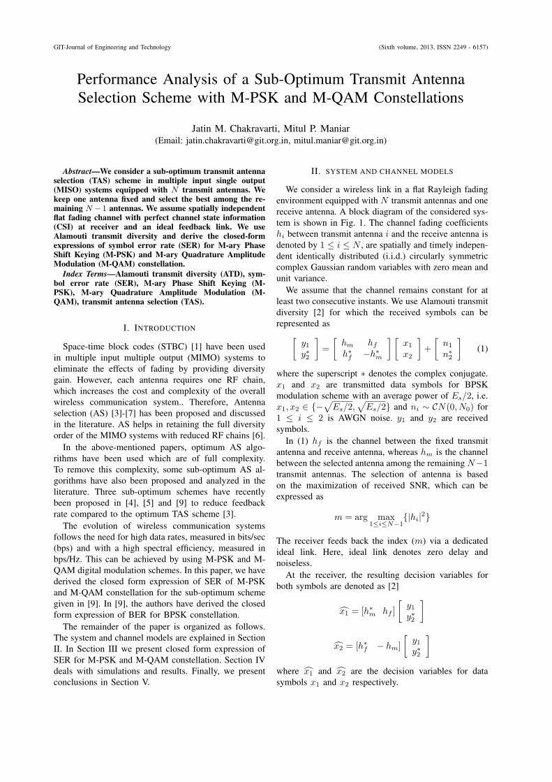
GIT-Journal of Engineering and Technology (Sixth volume, 2013, ISSN 2249 - 6157)
Performance Analysis of a Sub-Optimum Transmit AntennaSelection Scheme with M-PSK and M-QAM Constellations
Jatin M. Chakravarti, Mitul P. Maniar(Email: [email protected], [email protected])
Abstract—We consider a sub-optimum transmit antennaselection (TAS) scheme in multiple input single output(MISO) systems equipped with N transmit antennas. Wekeep one antenna fixed and select the best among the re-maining N −1 antennas. We assume spatially independentflat fading channel with perfect channel state information(CSI) at receiver and an ideal feedback link. We useAlamouti transmit diversity and derive the closed-formexpressions of symbol error rate (SER) for M-ary PhaseShift Keying (M-PSK) and M-ary Quadrature AmplitudeModulation (M-QAM) constellation.
Index Terms—Alamouti transmit diversity (ATD), sym-bol error rate (SER), M-ary Phase Shift Keying (M-PSK), M-ary Quadrature Amplitude Modulation (M-QAM), transmit antenna selection (TAS).
I. INTRODUCTION
Space-time block codes (STBC) [1] have been usedin multiple input multiple output (MIMO) systems toeliminate the effects of fading by providing diversitygain. However, each antenna requires one RF chain,which increases the cost and complexity of the overallwireless communication system.. Therefore, Antennaselection (AS) [3]-[7] has been proposed and discussedin the literature. AS helps in retaining the full diversityorder of the MIMO systems with reduced RF chains [6].
In the above-mentioned papers, optimum AS algo-rithms have been used which are of full complexity.To remove this complexity, some sub-optimum AS al-gorithms have also been proposed and analyzed in theliterature. Three sub-optimum schemes have recentlybeen proposed in [4], [5] and [9] to reduce feedbackrate compared to the optimum TAS scheme [3].
The evolution of wireless communication systemsfollows the need for high data rates, measured in bits/sec(bps) and with a high spectral efficiency, measured inbps/Hz. This can be achieved by using M-PSK and M-QAM digital modulation schemes. In this paper, we havederived the closed form expression of SER of M-PSKand M-QAM constellation for the sub-optimum schemegiven in [9]. In [9], the authors have derived the closedform expression of BER for BPSK constellation.
The remainder of the paper is organized as follows.The system and channel models are explained in SectionII. In Section III we present closed form expression ofSER for M-PSK and M-QAM constellation. Section IVdeals with simulations and results. Finally, we presentconclusions in Section V.
II. SYSTEM AND CHANNEL MODELS
We consider a wireless link in a flat Rayleigh fadingenvironment equipped with N transmit antennas and onereceive antenna. A block diagram of the considered sys-tem is shown in Fig. 1. The channel fading coefficientshi between transmit antenna i and the receive antenna isdenoted by 1 ≤ i ≤ N , are spatially and timely indepen-dent identically distributed (i.i.d.) circularly symmetriccomplex Gaussian random variables with zero mean andunit variance.
We assume that the channel remains constant for atleast two consecutive instants. We use Alamouti transmitdiversity [2] for which the received symbols can berepresented as[
y1y∗2
]=
[hm hf
h∗f −h∗
m
] [x1
x2
]+
[n1
n∗2
](1)
where the superscript ∗ denotes the complex conjugate.x1 and x2 are transmitted data symbols for BPSKmodulation scheme with an average power of Es/2, i.e.x1, x2 ∈ −
√Es/2,
√Es/2 and ni ∼ CN(0, N0) for
1 ≤ i ≤ 2 is AWGN noise. y1 and y2 are receivedsymbols.
In (1) hf is the channel between the fixed transmitantenna and receive antenna, whereas hm is the channelbetween the selected antenna among the remaining N−1transmit antennas. The selection of antenna is basedon the maximization of received SNR, which can beexpressed as
m = arg max1≤i≤N−1
|hi|2
The receiver feeds back the index (m) via a dedicatedideal link. Here, ideal link denotes zero delay andnoiseless.
At the receiver, the resulting decision variables forboth symbols are denoted as [2]
x1 = [h∗m hf ]
[y1y∗2
]
x2 = [h∗f − hm]
[y1y∗2
]where x1 and x2 are the decision variables for datasymbols x1 and x2 respectively.

GIT-Journal of Engineering and Technology (Sixth volume, 2013, ISSN 2249 - 6157)
III. PERFORMANCE ANALYSIS
In this section, using closed form expression of re-ceived SNR in [9], we obtain exact expression of SERfor M-PSK and M-QAM constellations.
We assume that both x1 and x2 are equally probable.Hence, we can express the instantaneous SNR (γ) perbit as
γ = ∥H∥2γc (2)
where H = [hm hf ]T and γc = Es/2No. Now, the pdf
of γ is derived in [9] as
pγ (γ) =N − 1
γc
[γ
γc
e− γ
γc +N−2∑k=1
(−1)k
(1
k
)(N − 2
k
)e− γ
γc − e− γ(1+k)
γc
](3)
A. SER for M-ary PSK Modulation
The SER for M-PSK constellation can be representedas [13]
Pe =1
π
∫ π(M−1)M
θ=0
∫ ∞
γ=0
pγ(γ)e− sin2(π/M)γ
sin2(θ) dγ.dθ (4)
where M is the number of symbols transmitted. SERcan be derived by substituting (3) in (4)
Pe = N − 1
[M − 1
M− 1
π
√C1
1 + C1
(π
2+ tan−1(α1)
)
×
(1 +
1
2(1 + C1)
)− sin(2 tan−1(α1))
4(1 + C1)
+
N−2∑k=1
× (−1)k
k
(N − 2
k
)(M − 1
M
)[1−
√C2
1 + C2
×
(M
(M − 1)π
)(π
2+ tan−1(α2)
)]−
N−2∑k=1
× (−1)k
k(1 + k)
(N − 2
k
)(M − 1
M
)[1−
√C3
1 + C3
×
(M
(M − 1)π
)(π
2+ tan−1(α3)
)]], (5)
where
C1 = C2 = γc sin2(π/M);
C3 =γc
1 + ksin2(
π
M);
αi =
√Ci
1 + Cicot(
π
M), 1 ≤ i ≤ 3.
For the special case of M = 2 (BPSK), the aboveexpression matches the equation no. (9) of [9]
Fig. 1. Block diagram of an Alamouti transmit diversity system withsub-optimum (N, 2; 1) TAS scheme
B. SER for M-ary QAM Modulation
The SER for M-QAM constellation can be representedas [13]
Pe =4
π
(1− 1√
M
)∫ π2
0
∫ ∞
0
pγ(γ)e− 3γ
2(M−1) sin2(θ) dγdθ
− 4
π
(1− 1√
M
)2 ∫ π4
0
∫ ∞
0
pγ(γ)e− 3γ
2(M−1) sin2(θ) dγdθ
(6)
where M is the number of symbols. SER can be derivedby substituting (3) in (6)
Pe = D − E, (7)
where D is shown as below
D = 4(N − 1)
(1− 1√
M
)[1
2− 1
π
√C1
1 + C1
×
(π
2+ tan−1(α1)
)(1 +
1
2(1 + C1)
)
− sin(2 tan−1(α1))
4(1 + C1)
+
N−2∑k=1
(−1)k
2k
(N − 2
k
)
×
[1−
√C2
1 + C2
(2
π
)(π
2+ tan−1(α2)
)]
−N−2∑k=1
(−1)k
2k(1 + k)
(N − 2
k
)[1−
√C3
1 + C3
×
(2
π
)(π
2+ tan−1(α3)
)]],
where
C1 = C2 =3γc
2(M − 1);
C3 =3γc
2(M − 1)(1 + k);
αi =
√Ci
1 + Cicot(
π
2), 1 ≤ i ≤ 3,

GIT-Journal of Engineering and Technology (Sixth volume, 2013, ISSN 2249 - 6157)
and E is shown as below
E = 4(N − 1)
(1− 1√
M
)2[1
4− 1
π
√C1
1 + C1(π
2+ tan−1(α1)
)(1 +
1
2(1 + C1)
)
− sin(2 tan−1(α1))
4(1 + C1)
+
N−2∑k=1
(−1)k
4k
(N − 2
k
)
×
[1−
√C2
1 + C2
(2
π
)(π
2+ tan−1(α2)
)]
−N−2∑k=1
(−1)k
2k(1 + k)
(N − 2
k
)
×
[1−
√C3
1 + C3
(2
π
)(π
2+ tan−1(α3)
)]],
where
C1 = C2 =3γc
2(M − 1);
C3 =3γ
c
2(M − 1)(1 + k);
αi =
√Ci
1 + Cicot(
π
2), 1 ≤ i ≤ 3.
IV. RESULTS
In this section, we show the analytical results obtainedin section III. We denote the considered sub-optimumsystem as (N, 2; 1), which indicates that two transmitantennas are selected from N with one receive antenna.Fig. 2 shows the SER for N = 3, 4 and 5 using M-PSK constellation. We have carried out the simulationfor M = 2 and 4, also known as BPSK and QPSKrespectively. It can be seen that the SER performance ofBPSK is better than that of QPSK, but spectral efficiencycan be achieved in the latter case. It can also be observedthat performance has been improved for larger values ofN .
Fig. 3 shows the SER for N = 3, 4 and 5 using M-QAM constellation. We have carried out the simulationfor M = 16 and 64, also known as 16-QAM and64-QAM respectively. It can be seen that the SERperformance of 16-QAM is better than that of 64-QAM,but spectral efficiency can be achieved in the lattercase. It can also be observed that performance has beenimproved for larger values of N .
V. CONCLUSION
We have considered the sub-optimum transmit antennaselection scheme given in [9]. In this scheme we have Ntransmit antennas in MISO systems, wherin one antennais fixed and the other is selected out of the remainingN − 1 antennas. We have derived the closed-form ex-pressions of SER of M-PSK and M-QAM constellation
2 4 6 8 10 12 14 1610
−6
10−5
10−4
10−3
10−2
10−1
100
Avg. SNR dB
SE
R
(3,2;1)(4,2;1)(5,2;1)
BPSK
QPSK
Fig. 2. SER Vs Avg. SNR for M-PSK constellation
2 4 6 8 10 12 1410
−2
10−1
100
Avg. SNR dB
SE
R
(3,2;1)
(4,2;1)
(5,2;1)
16−QAM
64−QAM
Fig. 3. SER Vs Avg. SNR M-QAM constellation
for Alamouti transmit diversity. We have compared ouranalytical results for higher values of M for M-PSK andM-QAM constellation. We achieve spectral efficiencyas the value of M increases with some performancedegradation in terms of SER.
REFERENCES
[1] V Tarokh, H. Jafarkhani and A.R.Calderbank, “Space-time blockcodes from orthogonal designs,” IEEE Trans. Inform. Theory, vol45, pp. 1456-1467, July 1999.
[2] S. M. Alamouti, “A simple transmit diversity technique for wire-less communications,” IEEE J. Selected Areas Communications,vol. 16, pp. 1451-1458, October 1998.
[3] Z. Chen, J. Yuan, B. Vucetic and Z. Zhou, “Performance ofAlamouti scheme with transmit antenna selection,” ElectronicsLetters, vol. 39, No. 23, pp. 1666-1668, November 2003.
[4] Z. Chen, I. B. Collings, Z. Zhuo and B. Vucetic, “TransmitAntenna Selection Schemes with Reduced Feedback Rate,” IEEETrans. Wireless Communications, vol. 8, No. 2, pp 1006-1016,February 2009.
[5] Y N Trivedi , A K Chaturvedi, “Performance analysis of AlamoutiScheme with Transmit Antenna Selection in MISO Systems,” Na-tional Conference on Communications (NCC), IIT Madras,2010.

GIT-Journal of Engineering and Technology (Sixth volume, 2013, ISSN 2249 - 6157)
[6] D. A. Gore and A. Paulraj, “MIMO antenna subset selection withspace-time coding,” IEEE Trans. Signal Processing, vol 50, No.10, pp. 2580-2588, October 2002.
[7] D. J. Love, “On the Probability of Error of Antenna-SubsetSelection With Space-Time Block Codes,” IEEE Trans. Commu-nications, vol. 53, No. 11, pp. 1799-1803, November 2005.
[8] “Physical layer procedures (FDD),” 3rd Generation PartnershipProject (3GPP), Tech. Rep. 25.214, 2005.
[9] J. M. Chakravarti, Y. N Trivedi, “Performance Analysis ofAlamouti Transmit Diversity with Transmit Antenna Selection forReduced Feedback Rate,” ICDeCom-11, BIT Mesra (Ranchi),India, February 2011.
[10] A. Papoulis and S. U. Pillai, Probability, Random Variables andStochastic Processes, 4th ed. MH.
[11] J G Proakis, Digital Communication, 4th ed. MH, 2001.[12] H. A. David, Order statistics, New York Wiley, 1970.[13] M K Simon and M S Alouini, Digital communication over fading
channels -A unified approach to performance analysis, John Wiley& Sons, 2000.

GIT-Journal of Engineering and Technology (Sixth volume, 2013, ISSN 2249 – 6157)
COMPARISION OF DIFFERENT EDGE BASED
ACTIVE CONTOUR MODELS AND THEIR
SOLUTION FOR IMAGE SEGMENTATION
1Asst. Prof. Dhaval R. Sathawara,
2 Asst. Prof. Margam K. Suthar,
3Mr.Bharat P. Solanki
1Department of Electronic and Communication Engineering
U.V.Patel collage of engineering, Ganpat university Kherva (Mehsana), India
2Department of Electronic and Communication Engineering,
Sankalchand Patel collage of engineering, visnagar (Mehsana), India
3Department of Electronic and Communication Engineering,
Student M.Tech [L. D. collage of engineering, Gujarat Technological university (Ahmedabad), India
Abstract—Image segmentation is one of the most important steps
in the image analyses. Its aim is to divide image in some parts
which correlate strongly by objects. Segmentation is difficult task
because of big variety of object, shape as well as different quality.
In t h i s paper various models of finding active contour is
discussed. First two methods of image segmentation are based on
principle paradigm of edge or gradient by minimizing the energy
of an image. Later section discuss about the practical limitation
of the models. Another paradigm is that the detection of active
contour whose stopping term does not depend on the gradient.
Later on we discuss how this method is advantageous or more
beneficial in finding the interested regions from an image.
I. INTRODUCTION
Active contours are used in the domain of image
processing to locate the contour of an object. Trying to locate
an object contour purely by running a low level image
processing task such as canny, sobel and prewitt edge
detections are not particularly successful. Often the edge is not
continuous, i.e. edges are broken or not connected, and
spurious edges can be present because of noise. An active
contour tries to improve on this by imposing desirable
properties such as continuity and smoothness to the contour of
the object.
In section II, discussion of the basic active contour method
which is introduced in “international journal of computer
vision”. How image is segmented based on minimizing energy
terms and how it can be formulated in different energy terms.
Section III, introduce new model to overcome limitations of
previous model. Section IV, involve model of active contour
detection which is not depend on edge rather than depending
on level set function. Section V, experimental results are
discussed for selecting the model which satisfy requirement
for application.
II. SNAKE OR CLASSICAL ACTIVE CONTOUR BY KASS
The concept of active contours models was first introduced
in 1987 [1] and has later been developed by different
researchers. An active contour is an energy minimizing that
detects specified features within an image. It is a flexible
curve which can be dynamically adapted to required edges or
objects in the image.
Figure 1. Illustration of a parametric snake curve v(s). The blue dot marks the
starting point and end point of the snake curve [2].
The position of the snake is given by the parametric curve v(s)
= [x(s); y(s)]T
with S [0; 1],in practice the curve is
often closed which means that v(0) = v(1). Furthermore the
curve is assumed to be parameterized by arc length. A closed
parametric snake curve is illustrated in Fig. 1. Each point
along the curve is under the influence of both internal and
external forces [2]. Fitting active contours to shapes in image
is an interactive process. The contour will then be attracted to
Features in the image extracted by internal energy creating an
attractor image [3].
The active contour model that Kass et al. introduced was
further developed by Laurent D. Cohen in the paper\On Active
Contour Models and Balloons". The snake model that Cohen

GIT-Journal of Engineering and Technology (Sixth volume, 2013, ISSN 2249 – 6157)
presents in the paper works on the same principles as the Kass
et al. snake, but where the Kass et al. snake would shrink
when not under the influence of image forces the Cohen snake
Expands. The expansion of the snake bears some resemblance
to a balloon being inflated in 2D, which is why this snake
model is usually called the balloon snake [6].
A. The Original Snake by Kass, Witkin & Terzopoulos
Snakes, developed by Kass et al. [1], is a method of
molding a closed contour to the boundary of an object in an
image. The snake model is a controlled continuity closed
contour that deforms under the influence of internal forces,
image forces, and external constraint forces. The internal
contour forces provide a piecewise smoothness constrain [4].
Kass et al. introduced the following energy functional for
calculating the snake energy
The snake energy consists of three terms. The first term represents the internal energy of the snake while the
second term denotes the image forces; the last term
Gives rise to external constraint forces [2]. The sum
of the image forces And the external constraint forces
is also simply known as the external snake forces,
denoted by . The internal energy of the snake is written
Where, the first-order term gives a measure measure
of the curvature. This means that in parts of the snake where
the curve is stretched, the elasticity term will have a high
value, while in parts of the snake where the curve is kinked;
the curvature term will have a high value. The influence that
these terms have on the overall snake energy is controlled by
the confidents and . The image forces attract
the snake to the desired features in the image. If the snake
should settle on edges in the image, then the image energy can
be defined as , with I being the image
function. Thus the snake will position itself in parts of the
image with high gradient values. The external constraint forces
are attributed to some form of high level image
understanding, most likely defined by human interaction [2]. The external energy consists of both the image energy
and the external constraint forces ,
however in order to simplify the analysis we will disregard the
external constraint forces.
B. The image energy forces
Let us take closer look at the image
energy . A crucial step in the Snake model is
finding a suitable term for the image energy; this is
because the snake will try to position itself in areas of low
energy. Often the snake should be attracted to edges in the
image and when this is the case a suitable energy term is
, where I is the image function. In
order to remove noise from the image and increase the
capture range of the snake. The image can be convolved
with a Gaussian kernel before computing the gradients.
This gives the following image energy term
Where is a two dimensional Gaussian with
standard deviation . When strong edges in the image are
blurred by the Gaussian the corresponding gradient is also
smoothed which results in the snake coming under the
influence of the gradient forces from a greater distance,
hereby increasing the capture range of the snake
C. The internal energy of the sanake
The internal energy of the snake is defined as in (2). As
The first order term measures the elasticity of the
snake, while the second order term measures the
curvature energy. The influence of each term is controlled
by the coefficients and . The more the snake is
stretched at a point v(s) the greater the magnitude of the
first order term, whereas the magnitude of the second order
term will be greater in places where the curvature of the
curve is high. It should be noted that if the snake is not
under the influence of any image energy, and only moves
to minimize its own internal energy. Then, for a closed
curve, it will take the form of a circle that keeps shrinking
and for a open curve the snake will position itself to form a
straight line that also shrinks. The internal forces of the
snake are however necessary in order to preserve desirable
properties such as continuity and smoothness of the curve
[2].
III. THE GREEDY SNAKE ALGORITHM
To improve and correct some of the problems
associated with the Kass et al. snake model D. J. Williams
and M. Shah developed a snake algorithm dubbed the
Greedy snake. One of the problems is that the snake
control points in the Kass et al. snake model are not always
evenly spaced. Sometimes the snake control points bunch
up in areas of the contour where the image energy has high
negative values. This behaviour causes problems with
calculating the curvature since the assumption that the
snake parameter is arc length will not hold if the snake
points are not equally spaced. The Greedy snake algorithm
also introduce the problem of numerical instability that
might occur if the temporal step size of the Kass et al.
snake is too large. Furthermore, problems arising from the
finite difference approximations for the elasticity and
curvature terms are evaluated and new discrete
approximations are suggested

GIT-Journal of Engineering and Technology (Sixth volume, 2013, ISSN 2249 – 6157)
A. Evaluating the image energy
The image energy of the Greedy snake is calculated same
as the image energy is calculated in snake by Kass with a quite
different
Which is almost the same energy term as in the Kass et al.
snake except that there is missing a minus in front of the term.
The Greedy snake algorithm works by examining the
neighbourhood around each snake point and then moving to the
position with the lowest energy. Therefore the image energy in
the neighbourhood of the snake control point has to be
normalized in a manner which assigns large negative values to
pixels with high gradient values, while assigning lower negative
values to pixels with a lower gradient value. The gradient
magnitudes are all in the interval [0; 255]. The normalization of
the neighbourhood is calculated as
is the minimum gradient value in the neighborhood.
is the maximum and the gradient magnitude of
the current point. This normalization sets the highest gradient
magnitude in the neighbourhood to -1 and the lowest to 0. One
problem with this method is that if the neighbourhood is nearly
uniform in gradient magnitude we get large difference in the
normalized values [2].
B. Elastic term of greedy
snake
As mentioned by Kass et al. snake the elasticity term
has the effect of causing the curve to shrink upon
itself. The Greedy snake utilizes a different way of calculating
the elasticity term. Thus reducing the shrinking effect and also
making sure that the snake control points does not bunch up in
places with high image energy. The elasticity term in the
Greedy snake is calculated in the neighbourhood of each snake
control point as
Where d is the average distance between all the points in
the snake. Once the above term has been calculated for each
pixel in the neighbourhood of a snake control point all the
values are divided by the largest value in the neighbourhood.
Which means that the neighbourhood is normalized so, it only
contains elasticity term values between [0; 1]. The minimum
energy will be achieved when
Equation (7) will be true for all points where, the
average distance equals the distance between the current and
previous point on the snake.

GIT-Journal of Engineering and Technology (Sixth volume, 2013, ISSN 2249 – 6157)
IV. ACTIVE CONTOUR USING LEVEL SET FUNCTION
All these classical snakes and active contour models rely
on the edge function, depending on the image gradient, to stop
the curve evolution; these models can detect only objects with
edges defined by gradient. In practice, the discrete gradients
are bounded and then the stopping function is never zero on
the edges, and the curve may pass through the boundary,
especially for the model in [1], [8]-[10]. If the image is very
noisy, then the isotropic smoothing Gaussian has to be strong
which will smooth the edges. In this section, we propose a
different active contour model, without a stopping edge
function, i.e. a model which is not based on the gradient of the
image for the stopping process. The stopping term is based on
Mumford–Shah segmentation techniques. In this way, we
obtain a model which can detect contours both with and
without gradient, for instance objects with very smooth
boundaries or even with discontinuous boundaries. In addition,
our model has a level set formulation, interior contours are
automatically detected, and the initial curve can be anywhere
in the image [7].
A. Energy function and Lipschitz dunction
Our method is the minimization of an energy based-
segmentation. Let us first explain the basic idea of the model in
a simple case. Assume that the image is formed by two
regions of approximately piecewise-constant intensities, of
distinct values and . Assume further that the object to be
detected is represented by the region with the value . Let
denote its boundary by . Then we have inside the
object and outside the object. Now let us consider the
following “fitting” term:
This can be seen easily. For instance, if the curve is
outside the object, then and . If the
curve is inside the object, then but . If
the curve is both inside and outside the object, then
and . Finally, the fitting energy is
minimized if , i.e., if the curve is on the boundary of
the object. These basic remarks are illustrated in figure 2.
Figure 2. All possible cases in the position of the curve. The fitting term is minimized only in the case when the curve is on the boundary of object [7].
In the Level set method, is represented by the zero
Level set of a Lipschitz function , such that
For the Level set formulation of our variation active
contour model, we replace the unknown variable by the
unknown variable . Using the Heaviside function H, and the
one-dimensional Dirac measure , and defined, respectively,
by
Then, the energy can be written as
We note that, as defined earlier, solution of our model as a
particular case of the Mumford–Shah minimal partition
problem, can simply be written using the Level set formulation
as
Keeping fixed and minimizing the energy
with respect to the constants and , it is easy to express these
constants function of by
If (i.e. if the curve has a nonempty
interior in ), and

GIT-Journal of Engineering and Technology (Sixth volume, 2013, ISSN 2249 – 6157)
Here, c1 and c2 are the average intensity within the
objects and outside the objects respectively .Thus we can
define boundary of objects by function rather than the edge of
an image.
B. Algorithm for evaluating contour
In this model first we have to select initial region for better and fast result. Steps for evolving the contours are as follows:
Select Initial mask to calculate Initial
Compute and
Calculate Image force by image energy function.
Evaluate as:
Check whether the solution is stationary. If not then
increase n by n=n+1 and Repeat these steps.
V. EXPERIMENTAL RESULTS
We conclude this paper by analyze different models and their response for different types of Images. Sample image of a leaf is take to evaluate the contour by different models. Kass model is first step of field of contour evolving models but it does not have smooth curve. In greedy snake model, curvature is smooth but it not enough to exactly match the boundary of objects. Their model which is depend on Lipchitz function rather than edge provide complete boundary as well as it is less sensitive to high bending curvature as shown in Fig. 4.
Figure 4. Evaluating contour of binary Image by Kass, Greedy and Active contour using Lipchitz function column wise respectively.

GIT-Journal of Engineering and Technology (Sixth volume, 2013, ISSN 2249 – 6157)
Figure 5. Evaluating contour of Noisy gray scale Imageof std. dev=10 by Kass,
Greedy and Active contour using Lipchitz function column wise respectively.
Figure 5 shows different response of AWGN corrupted iamge.
Greedy is less sensitive to noise rather than Kass and third
model takes higher iteration to compote but it provide higher
accuracy compared to other two models.
Figure 6. Evaluating contour of Cygnusloop Xray image by Kass, Greedy and
Active contour using Lipchitz function column wise respectively.
Figure 6 shows that Kass model will neglect small objects and attract toward the larger object where in greedy model, small objects are grouped and consider as a one object and in third model all objects are consider separately rather than grouping.

GIT-Journal of Engineering and Technology (Sixth volume, 2013, ISSN 2249 – 6157)
separately where in third model separate boundary are extracted. And both contour are well separated not linked in one contour.
VI. CONCLUSION
In this paper we discuss about need of segmentation in image processing then we describe one domain of segmentation that is active contour detection. There are two approaches for detecting active contours, first two models (Ksaa and Greedy) are based on edge and third is independent of edge. A model of detecting active contour whose fitting term depends on the edge or gradient is very sensitive to noise. In such cases a model, which’s fitting term depend on the function rather than gradient will provide better and reliable results. Third model uses Lipchitz function to evaluate contour and gives better result with high accuracy as discussed in previous section. Thus active contour without gradient is better way to segment an image rather than gradient based model.
REFERENCES
[1] M. Kass, A. Witkin, and D. Terzopoulos, “Snakes: Active contour models,” Int. J. Comput. Vis., vol. 1, pp. 321–331, 1988.
[2] Nikolas Petteri Tiilikainen, “A Comparative Study of Active Contour Snakes”, 2007.
[3] Marian Bakos, “Active Contours and their Utilization at Image”, 5th
Slovakian-Hungarian Joint Symposium on Applied Machine Intelligence and Informatics January 25-26, 2007.
[4] William K. Pratt, “Digital Image Processing”, PIKS Inside, Third Edition.
[5] R. C. Gonzalez and R. E. Wood, ”digital image processing”, third edition. [6] Chenyang Xu and Jerry Prince,” an example of balloon model on the
room object”, 1996-97. [7] Tony F. Chan and Luminita A. Vese, ” Active Contours Without
Edges”, IEEE transactions on image processing, vol. 10, no. 2, february 2001.
[8] S. Kichenassamy, A. Kumar, P. Olver, A. Tannenbaum, and A. Yezzy, “Gradient flows and geometric active contour models,” in Proc. Int.Conf. Computer Vision, Cambridge, MA, 1995, pp. 810–815.
[9] M.-S. Lee and G. Medioni, “Inferred descriptions in terms of curves, regions and junctions from sparse, noisy binary data,” in Proc. IEEE Int. Symp. Computer Vision, Coral Gables, FL, 1995, pp. 73–78.
[10] R. Malladi, J. A. Sethian, and B. C. Vemuri, “Shape modeling with front propagation: A level set approach,” IEEE Trans. Pattern Anal. Machine Intell., vol. 17, pp. 158–175, Feb. 1995.
[11] Dhaval R. sathawara and Assist. Prof. Amrut N. Patel, “Image Segmentation Using Active Contour” International Conference on Information, Knowledge & Research in Engineering, Technology & Sciences-2012, Amoghsiddhi Education Society journal.
[12] Junmo Kim, Member, IEEE, John W. Fisher, III, Member, IEEE, Anthony Yezzi, Member, IEEE, Müjdat Çetin, Member, IEEE, and Alan S. Willsky, Fellow, IEEE, “A Nonparametric Statistical Method for Image Segmentation Using Information Theory and Curve Evolution”, IEEE Transactions On Image Processing, Vol. 14, No. 10, October 2005.
[13] Xavier Bresson, Selim Esedoḡlu, Pierre Vandergheynst, Jean-Philippe Thiran, Stanley Osher, “Fast Global Minimization of the Active Contour/Snake Model”, Journal of Mathematical Imaging and Vision, Volume 28, Issue 2, pp 151-167, June 2007.
[14] Chunming Li, Chenyang Xu, Senior Member, IEEE, Changfeng Gui, and Martin D. Fox, Member, IEEE, “Distance Regularized Level Set Evolution and Its Application to Image Segmentation”, IEEE Transactions On Image Processing, Vol. 19, No. 12, December 2010.
Figure 7. Evaluating contour of two object RGB image by Kass, Greedy and
Active contour using Lipchitz function column wise respectively.
Figure 7 shows nature of response of different models under
influence of image which contain two objects. Both Kass and Greedy models are not able to find boundary of those object

GIT-Journal of Engineering and Technology (Sixth volume, 2013, ISSN 2249 – 6157)
VineetaNishad ,JitendraThathagar
( [email protected], [email protected] )
Abstract—Smart grid is a next-generation electrical grid which
set up a high-speed, fully integrated, two way communication
technological frameworks having network features of dynamic
interaction, real-time information and power exchange. This
paper represents an end-to-end baseband model of the physical
layer of a WiMAX communication network according to the
IEEE® 802.16 standard. The model supports all mandatory and
optional data rates 27 Mb/s. The model also illustrates adaptive
modulation and coding over a flat-fading and dispersive
multipath fading channel, whereby the simulation varies the data
rate dynamically The channel estimation technique uses
training sequence inserted at the beginning of each
transmission. Theory and methods are presented in details.
The system model is designed for WiMAX IEEE 802.16
transceiver in MATLAB Simulink and the performances are
evaluated using software Matlab.
Index Terms— Adaptive modulation, Multipath Fading,
OFDM, Smart Grid,WiMAX.
I. INTRODUCTION
The conventional centrally controlled electrical grid is
facing challenges such as rising energy demand, aging
infrastructure, renewable energy sources, reliability and
security which necessitate it to evolve towards intelligence,
autonomy, improved efficiency, easy control, and high
security. The smart grid will be the next-generation electricity
grid and integrates emerging technologies in the areas of
embedded sensing, broadband wireless communication,
pervasive computing, and adaptive control. Cognitive Radio is
an efficient and reliable communication technology to
establish two-way information transmission between
customers and utilities.
In recent years, Mobile WiMAX has received wide interest
for next generation wireless communications. Two key
technologies, Multiple Input Multiple Output (MIMO) and
Orthogonal Frequency Division Multiplexing (OFDM) have
been adopted in Mobile WiMAX standard, IEEE 802.16e
(Mobile WiMAX) which is an extension of the IEEE 802.16-
2004, which enable high data rate transmission over multipath
and frequency selective fading channels Accurate channel
state information (CSI) is required to perform coherent
detection of OFDM signals and estimating mobile channels
for high data rate communications has proved to be very
challenging [10].
Channel estimation of MIMO-OFDM systems has been
widely investigated by researchers and two kinds of
approaches have been introduced, frequency and time domain
channel estimation. In these methods, a complete OFDM
frame composed of training symbols is first sent in order to
estimate the channel parameters. The channel is therefore
assumed to be constant for the next OFDM blocks until a new
estimation is performed. In fast fading environment,
performances degradation would be noticed due to the
outdated channel estimation. Normally, estimation performed
in time domain would be more appropriate as impulse
responses contain fewer parameters than frequency responses.
Simulations were conducted based on the specifications
given in the IEEE 802.16e standard for WiMAX and under
Stanford University Interim (SUI) channel models.
II. COMMUNICATION ARCHITECTURE IN SMART GRID
Three fundamental functionalities are desirable for the
communications infrastructure of the smart grid: sensing,
transmission, and control. Embedded sensing is carried out by
a large number of smart meters or sensors to detect the states
of the various points of the grid in a real-time manner. Two-
way transmission links should be established for data transport
between the sensors and the control centers. To fulfill these
purposes, the smart grid communications infrastructure has to
integrate enabling networking technologies. The smart grid is
usually deployed in a considerably large geographical field to
connect a large set of nodes. Therefore, the communication
infrastructure is envisioned to be a multilayer structure that
extends across whole smart grid from the home area to the
neighborhoodarea and the wide area (Fig. 1). In particular,
home area networks (HANs) communicate with various smart
devices to provide energy efficiency managementand demand
response. Neighborhood area networks (NANs)connect
multiple HANs to local access points. Wide area networks
(WAN) provide communication links between theNANs and
the utility systems to transfer information.
BER Performance of Equalized Signal in Wireless
Communication Architecture of Smart Grid

GIT-Journal of Engineering and Technology (Sixth volume, 2013, ISSN 2249 – 6157)
A.Proposed Three-Layered Structure
Fig.1 shows the proposed communication architecturebased on
cognitive radio (CR) for the smart grid. The communication
architecture adopts the three-tiered hierarchical structure,
including HAN, NAN, and WAN. On one hand, cognitive
communications that operate in the license-free bands are
appliedin the HAN to coordinate the heterogeneous wireless
technologies; on the other hand, cognitivecommunications
thatoperate in the licensed band are applied in the NAN
andWAN to dynamically access the unoccupied spectrum
opportunities.
B.Cognitive Communications in Home Area Networks
Topology — The HAN consists of a cognitive home gateway
(HGW), smart meters, sensors, actuators, and other intelligent
devices. A networked smart meter system is a typical instance
in a HAN to offer an energy-efficient and reliable next-
generation power grid. The presented HAN uses a star
topology with either wired technologies (e.g., power line
communications) or different wireless technologies (e.g.,
Zigbee, Bluetooth, WiMAX and WiFi). Consequently, HAN is
an essentially heterogeneous networkwith a number of
complementary technologies, which calls for a very flexible
service gateway to manage the communications within the
HAN and the communications between different HANs in a
NAN service range.
Dynamic Spectrum Sharing in Cognitive HANs — In this
sense, the HGW is able to intelligently interact with the radio
surroundings, adaptively connect, and change their
transmitters’ parameters. The radioagility capacity in the
HGW is able to sense unused frequencies in the surroundings
and can utilize them subject to interference constraints. In
addition, the HGW will connect to the HAN, which in turn
will connect to external networks (e.g., the Internet, NAN, or a
utility). The HGW enables two-way communications in the
HAN. In the forward direction, the HGW periodically collects
power-related data (e.g. metered data, sensed data, and load
and control information) from various
machines/devices/terminals within the HAN, and then
transfers the collected data outside of the NAN. In the
opposite direction, the HGW acts as a central node within the
cognitive NAN to receive data (e.g., pricing, demand
response) from the NAN and then distribute the received data
to the smart meters or display to the customers. Within a
HAN, the HGW manages the license-free spectrum bands to
provide optimal data rate with low interference. An efficient
solution to spectrum sharing among networked smart meters is
necessary. Apart from spectrum sharing management, the
HGW enables other devices and sensors to join the network,
assigns channel and network addresses to each device, and
coordinates the communications between thedevices within
the HAN.
Fig 1. Cognitive radio based hierarchical communications architecture in the smart grid.

GIT-Journal of Engineering and Technology (Sixth volume, 2013, ISSN 2249 – 6157)
C.Cognitive Communications in Neighborhood Area Networks
Topology — In smart grid applications, the NANs will collect
energy consumption information from households in a
neighborhood and deliver the information to a utility company
through either open or private WANs. NANs typically
comprise multiple utility meters, each of which is installed on
or outside of a house. In the proposed cognitive
communication architecture, a NAN is the next immediate tier
of a HAN. In a NAN, a cognitive gateway (NGW) connects
several HGWs from multiple HANs together, as shown in Fig.
1. The HGWs are the data access points of the HANs to the
outside NAN, and they also act as the cognitive nodes located
in the NAN.
D. Cognitive Communications in Wide Area Networks
Topology — Fig.1 shows that multiple NANs constitute a
WAN, andeach NAN exchanges information with the utility
control center through the WAN. In the WAN, each NGW is
no longeran access point, but a cognitive node with the
capability tocommunicate with the control center through
frequency spaceunused by a licensed PU. The control center is
connected withcognitive radio base stations that are dispersed
over a largearea (e.g., a city). In conjunction with the control
center, thereis a spectrum broker that plays an important role
in sharingthe spectrum resources among different NANs to
enablecoexistence of multiple NANs. The cognitive radio base
stations manage the communications of the NGW. In a
largegeographical distribution of NANs, several NGWs may
not bewithin the geographic area covered by base stations.
TheseNGWs have to communicate in an ad hoc mode to
shareunoccupied spectrum bands by themselves.To improve
the spectrum efficiency and reduce the cost ofbuying spectrum
bands, licensed and unlicensed accessmodes are intelligently
scheduled and seamlessly switched.The smart grid user (or
service) is not aware of the actualaccess mode it is using.
E. Cross-Layer Spectrum Sharing in HAN
Smart meters and intelligent sensors and actuators in
homeareas are networked for information collection and
delivery toconstitute the HAN of the smart grid. As mentioned
before,different wireless technologies may be adopted by
variousmeters/sensors/actuators, and hence coexist in a HAN.
Thespectral overlay between these wireless systems may
causesevere interference to each other and deteriorate
systemcapacity. Thus, cognitive spectrum sharing is necessary
tocoordinate the spectrum access of the heterogeneous
wirelesssystems. Here, an HGW-assisted cross-layer cognitive
spectrum sharing mechanism is proposed.The mechanism has
two main components: the spectrumaccess controller and
power coordinator, which operate at themedium access control
(MAC) and physical (PHY) layers,respectively. Each wireless
node in a HAN is allowed toaccess the spectrum only if it is
permitted by the access controller.
F. Power Coordination
Consider a HAN with Iwireless nodes (e.g., smart
meters,sensors, or actuators) intending to transmit data. The
achievable rate of the ith
node is given by Shannon’s formula,
(1)
where Bi is the channel bandwidth, and pi(f) and N0 arethe
power spectral density (PSD) function of system i and noise in
receivers, respectively. The utility function of the ith
node is
defined by
(2)
G. Spectrum Access Control
Within the HAN, the cognitive HGW manages thespectrum
bands allocation and sharing to provide optimal data rate with
low interference. The spectrumaccess controller aims to
guarantee the QoS of all in-servicewireless nodes (i.e.,
players) by controlling the number of newplayers. If the
presence of a new player significantly degradesthe achievable
rate of one or more existing players, the newplayer shall be
blocked. Fig.2 shows four phases in thespectrum access
control:
Fi
g.2 HGW-assisted cross-layer spectrum sharing in a HAN.

GIT-Journal of Engineering and Technology (Sixth volume, 2013, ISSN 2249 – 6157)
Phase 1: The access control procedure is launched by the new player
that sends an access request to the HGW.
Phase 2: The access controller passes the profile of the new player to
the power coordinator. The profile contains the information of the
specific parameters of the utility function and the PSD function of the
new players.
Phase 3: The power coordinator analyzes and obtain the optimal
power control of all players (including the new one) The resulting
power control and achievable rate are fed back to the access
controller.
Phase 4: If one or more players reach an undesirable rate the new
player is denied; otherwise, it is admitted. The access controller
informs the new player of the admission/rejection decision, and all
the players about whether to update the transmitting power. Denied
players may retry to access later.
H. Joint WAN/NAN Spectrum Management
The spectrum management of the WAN and NANs should be jointly
optimized for the following main reasons:
• In most situations, all the NANs in the same WAN operate in the
same range of spectrum bands. There are underlying competitions on
spectrum resource among the NANs, which need overall
coordination.
• Different NANs have diverse demands on the amount of spectrum
bands, due to the difference in the total number of HANs and traffic
flows of HANs caused by the diversity in quantity and category of
smart meters/sensors/actuators.
We consider a WAN with k NANs. Let NlG,k, Nu
G,k, NlC,k,andNu
C,k
denote the number of licensed and unlicensed guard channels (GCs),
and licensed and unlicensed common channels of the kth NAN. Let
Pd,k, Pb,k denote the dropping probability and blocking probability of
the kth NAN, and Nk the number of allocated total channels of the
kthNAN. The joint WAN/NAN spectrum management could be
formulated as the following optimization problem:
(3)
The target is to find the optimal spectrum allocation scheme with
parametric tuples Nk, NlG,k, N
uG,k, N
lC,k, N
uC,k for all NANs. Fig.3
shows the performance gain of the proposed cognitive
communications infrastructure at the NAN and WAN level. It is
observed that the proposed scheme achieves much lower dropping
probability than the traditional solution. By using joint NAN/WAN
spectrum management, the cognitive infrastructure is aware of the
diversity of traffic load in different NANs, and consequently is able
to intelligently allocate the spectrum bands. As a consequence,
spectrum resources (both licensed and unlicensed) are utilized in a
highly efficient manner.
Fig.3 Performance comparison in a NAN between traditional
and proposed CR communications infrastructures for the smart grid.
III. WIRELESS COMMUNICATION SYSTEM MODEL
OFDM system works on the principle of division of the available
frequency spectrum into several subcarrier channel frequencies. The
subcarriers are orthogonal in nature and hence overlapping is possible
to achieve better spectral efficiency. Even though the signal passes
through a time dispersive fading channel, orthogonality can be
completely maintained with a small price in a loss in SNR[11].
A block diagram of a WiMAX OFDM PHY system is shown in Fig.
4[4]. The random binary signal information is first generated and
grouped in symbols, then coded for error correction. Adaptive
modulation system is used because different modulation scheme is
needed for different data rates. After that guard band is inserted and
the Inverse Fast Fourier Transform (IFFT) block transforms the data
sequence into time domain. If multiple antennas are used, then space-
time diversity encoder is also implemented. Then a cyclic prefix is
used which is chosen larger than the expected delay spread to avoid
inter-symbol and inter-carrier interferences (ISI and ICI). The D/A
converter contains low-pass filters withbandwidth 1/TS, where TS is
the sampling interval. The channel is considered to be a multipath
fading channel followed by addition of white Gaussian noise.
At the receiver, after passing through the analog-to-digital converter
(ADC) and removing the CP, the FFT is used to transform the data
back to frequency domain. Adaptive filtering technique is used for
channel estimation. Lastly, the binary information data is obtained
back after the demodulation and channel decoding.
1.1 Forward Error Correction Code
Digital communications need forward error correction (FEC) code
for reducing errors due to noise, fading, interference, and other
channel impairments. It is also called channel coding or error control
coding. It introduces controlled redundancies to a transmitted signal
so that they may be exploited at the receiver. The redundancy of the

GIT-Journal of Engineering and Technology (Sixth volume, 2013, ISSN 2249 – 6157)
encoded data is quantified by the ratio of bd data bits per bc
encoded bits
This ratio is known as the code rate, which basically means
for every bd data bits input into the encoder, there will be bc
code bits output from the encoder. Generally, correction codes
are categorized into two main types: block codes and
convolutional codes. Block coding is basically generating a
―codeword‖ of bc coded bits that would be algebraically
related to a sequence of bd data bits. Convolutional coding is
generated by the discrete-time convolution of a continuous
sequence of input data bits. Both block code and convolutional
code are employed in wireless systems. However,
convolutional codes have proven superiority over block codes
for a given degree of decoding complexity[14].
Fig. 4 IEEE 802.16 WiMAX - OFDM PHY system model in MATLAB Simulink[4].
1.2 Block Interleaving
The decoder operates under the assumption that the errors will be
random or spaced apart. However, in fading channels, deep fades
may cause a long sequence of errors, which may render the decoder
ineffective. In order to alleviate bit correlation, the encoded bits are
scrambled with a block interleaver (fig.5). Interleaving can either be
done before symbol mapping, and is known as bit interleaving, or it
can be done after symbol mapping, and is known as symbol
interleaving . The purpose of interleaving is to minimize the bit
correlation, while data symbols are essentially groups of bits.
Maintaining the bits in groups, in a sense, adds to the bit correlation,
especially when using larger constellations[11].
1.3 Modulation Schemes
Adaptive modulation systems improve the rate of transmission.
The implementation of adaptive modulation isaccording to the
channel information that is present at the transmitter.
Fig. 5 Transmission with a burst error and interleaving.
TABLE I. IEEE 802.16 TRANSMISSION MODES
Mode
or
Rate_I
D
Modul-
ation
Interlea-
ving
Code
Rate
Data
Rate
(Mbp
s)
Simulation-
Threshold
SNR (dB)
0
1
BPSK
BPSK
6 x 8
6 x 8
1/2
3/4
3
4.5
0
10
2
3
QPSK
QPSK
12 x 8
12 x 8
1/2
3/4
6
9
11
14
4 5
16-QAM 16-QAM
12 x 16 12 x 16
1/2 3/4
12 18
18 22
6
7
64-QAM
64-QAM
18 x 16
18 x 16
2/3
3/4
24
27
26
28
The method of making adaptive modulation in this model is
according to the estimated SNR, a bit rate will be specified
and then data source generates binary data according to the
specified data rate in adaptive modulation control. The
transmission modes supported in the IEEE 802.16 standard are
described in the Table 1.
1.4 OFDM Transmitter
OFDM converts serial data stream into parallel blocks of
size N and modulates these blocks using inverse fast Fourier

GIT-Journal of Engineering and Technology (Sixth volume, 2013, ISSN 2249 – 6157)
transform (IFFT). Time domain samples of an OFDM symbol
can be obtained from frequency domain data symbols [15] as
where X(i,k) is the transmitted data symbol at the k
th
subcarrier of the ith
OFDM symbol, N is the fast Fourier
transform (FFT) size. After the addition of cyclic prefix (CP)
and D/A conversion, the signal is passed through the radio
channel. The channel is assumed to be constant over an
OFDM symbol, but time-varying across OFDM symbols.
At the receiver, the signal is received along with noise.
After synchronization, down-sampling, and removal of the
CP, the simplified baseband model of the received samples
can be formulated[15] as
where L is the number of sample-spaced channel taps, w (n
) is the additive white Gaussian noise (AWGN) sample with
zero mean and variance of σ 2 , and the time domain channel
impulse response (CIR) for the current OFDM symbol, h (l ),
is given as a time-invariant linear filter. Note that perfect time
and frequency synchronization is assumed. In this case, after
taking FFT of the received signal y(n), the samples in
frequency domain can be written as
where H and W are FFTs of h and w respectively.
1.5 Pilot Insertion
An OFDM system is equivalent to a transmission of data
over a set of parallel channels. At the receiver, there are
equalizers for compensation of channel characteristics which
is achieved by sending pilot symbols from transmitter. Two
types of methods can be used for this as shown in fig.6.The
fading channel of the OFDM system can be viewed as a 2D
lattice in a time-frequency plane, which is sampled at pilot
positions and the channel characteristics between pilots are
estimated by using pilot information by the channel estimator
algorithm. The art in designing channel estimators is to solve
this problem with a good trade-off between complexity and
performance. The first one, block-type pilot channel
estimation, is developed under the assumption of slow fading
channel, and it is performed by inserting pilot tones into all
subcarriers of OFDM symbols within a specific period. The
second one, comb-type pilot channel estimation, is introduced
to satisfy the need for equalizing when the channel changes
even from one OFDM block to the subsequent one[11].
1.6 Training Sequence Preamble
The first symbol of each downlink subframe is dedicated as
a preamble in OFDMA mode of 802.16 standard. The
preamble is generated by modulating each third subcarrier
using boosted binary phase shift keying (BPSK) with a
specific pseudo noise (PN) sequence. Hence, the time domain
preamble consists of three repeating parts. This preamble is
used for initial estimation of time-varying channel[15].
Fig. 6 Two Basic Types of Pilot Arrangement for OFDM Channel Estimations
1.7 Equalization
A symbol-spaced linear equalizer consists of a tapped delay
line that stores samples from the input signal. Once per
symbol period, the equalizer outputs a weighted sum of the
values in the delay line and updates the weights to prepare for
the next symbol period. This class of equalizer is called
symbol-spaced because the sample rates of the input and
output are equal. Below is a schematic of a symbol-spaced
linear equalizer with N weights, where the symbol period is T.
Fig. 7 A linear equalizer with tapped delay line and N weights.
1.8 Radio Channel
There are three basic types of channels considered for this
work. Performance of three channels, viz., AWGN,
Rayleigh Fading Channel, Rician Fading Channel in
communication environment is evaluated through
simulation. Multipath fading is a significant problem in
communications. In a fading channel, signals experience fades
(i.e., they fluctuate in their strength). When the signal power
drops significantly, the channel is said to be in a fade.
This gives rise to high bit error rates (BER)[7].
1.9 Channel Estimation Time-dispersive channels can cause inter-symbol
interference (ISI), a form of distortion that causes symbols to
overlap and become indistinguishable by the receiver. For
example, in a multipath scattering environment, the receiver
sees delayed versions of a symbol transmission, which can
interfere with other symbol transmissions. An equalizer based
on LMS channel estimation algorithm attempts to mitigate ISI
and improve receiver performance.

GIT-Journal of Engineering and Technology (Sixth volume, 2013, ISSN 2249 – 6157)
IV. SIMULATIONS
In the realistic scenario where the channel state information
is not known at the receiver, this has to be extracted from the
received signal. We assume that the channel estimator
performs this using orthogonal pilot signals that are prepended
to every packet. It is assumed that the channel remains
unchanged for the length of the packet (i.e., it undergoes slow
fading).
Scatter plots of the received signal before and after
equalization are shown in each simulation. From the plot of
the equalized signal, modulation type the system can be
recognized, because the plot resembles a signal constellation
of 2, 4, 16, or 64 points. The power spectrum of the received
signal before and after equalization, in dB. The dynamics of
the signal's spectrum before equalization depend on the fading
mode parameter in the Multipath Channel block. The estimate
of the SNR based on the error vector magnitude. The bit rate
of the transmission is shown. Table II shows parameter values
for different simulations.
TABLE II
SIMULATION PARAMETERS IN ACCORDANCE WITH WIMAX 802.16 STANDARD
Carrier Frequency 2.3, 2.5, 3.5 GHz
Channel Model LOS/Non-LOS
Raw Bit Rate 1.0-75.0 Mbps
Modulation BPSK, QPSK, 16QAM, 64QAM
OFDM subcarriers 256
Channel Bandwidth 1.75, 3.5, 3, 7, 5.5, 10, 20 MHz
Frame Duration 5 ms
Number of Frames (per
second)
200
IFFT/FFT 256 point
Data Tone 192
Pilot tone 8
Cyclic Prefix 64
Guard Interval/Symbol
Interval
1/4, 1/8, 1/16, 1/32 (or 64, 32, 16,8
samples)
Decoder Viterbi
Fading Channel No fading; flat-fading; and Rayleigh
or Rician Multipath fading
Noise AWGN
TABLE III
SIMULATION RESULTS FOR VARYING PARAMETERS IN WIMAX SYSTEM MODEL
Case
No.
OFDM
symbols/block
OFDM
symbols/training sequence
SNR
(dB)
Doppler
Shift (Hz) Fading Mode Bit Rate (Mb/s)
PER
(%)
1. 200 8 20.44 200 No Fading 18 0
2. 200 8 19.67 50 Flat Fading 18 4
3. 200 8 4.119 200 Flat Fading 6 18
4. 50 8 13.89 200 Dispersive 12 14
5. 200 20 17.73 50 Dispersive 18 20
6. 500 8 15.89 50 Dispersive 12 34
7. 200 8 4.334 200 Dispersive 6 74
Fig. 8 shows the signal constellation and power spectrum of
received and equalized signal when there is no fading due to
channel. The SNR chosen is 20 dB and resultant bit rate is 18
Mbps but there are no packet errors. The received signal is
having distortion in amplitude only.
Fig. 9 shows the effect of flat fading channel with maximum
Doppler shift of 50 Hz. The signal is distorted in amplitude as
well as in phase but after equalization we can recognize the
signal. The power spectrum of received signal is flat. As we
vary the SNR values, bit rate is changed and error is generated
at 0 dB. Fig. 10 also shows the effect of flat fading channel but
maximum Doppler shift (200 Hz) is more than fig. 9 which
increases the packet error (18%), so BER performance is
relatively poor.
Fig. 11 through fig. 14 are having dispersive channel, which
means there is a multipath fading effect introduced in these
simulations. In fig. 8, the number of OFDM symbols/block
(50) is less as compared to other cases (200), so the number of
bits which are erroneous is least in this case because each
burst is having separate fading and noise effects. When the
length of block increases, a noise can deteriorate whole burst
block, so more number of data bits become erroneous.

GIT-Journal of Engineering and Technology (Sixth volume, 2013, ISSN 2249 – 6157)
Fig.8 Effect on received and equalized signal when there is no fading.
Fig.9 Effect of flat-fading channel on received and equalized signal
Fig.10 Effect on received and equalized signal when there is flat- fading
channel with more Doppler shift.
.
Fig.11 Effect of dispersive channel on received and equalized signal
In fig. 12 and 13, the received signal is distorted in amplitude
and phase due to multipath fading effects and the received
power spectrum is also varying. But after equalization, signal
constellation can be recognized and power spectrum is
balanced. Due to dispersive channel, SNR values continuously
changes, so bit rate is also changed. Number of training
symbols are more in case 5 (20) as compared to case 6 (8),so
equalization is better in case 5 and resultant erroneous bits are
less here.
Fig.12 Effect of multipath-fading channel on received and equalized
signal with more training symbols.
Fig. 14 shows the effect of signal to noise ratio upon bit rate and
packet error. When the SNR value of the signal goes below a
threshold level, the modulation scheme is changed for a transmission
with relatively lower bit rate. If the SNR value of the received signal
is too low, even after equalization the packet error rate is very high as
shown in the figure. The SNR value (4.334 dB) is minimum in case
7, so packet error (74%) is maximum here.

GIT-Journal of Engineering and Technology (Sixth volume, 2013, ISSN 2249 – 6157)
Fig: 13 Effect of multipath-fading channel on received and equalized
signal with more OFDM symbols per block.
Fig: 14Effect of signal to noise ratio upon bit rate and packet
error.
V. CONCLUSIONS
A MATLAB simulation is carried out in order to analyze
baseband processing of the transceiver. For this, IEEE 802.16
standard is applied which allows transmission data rates from
3 up to 27 Mbps. Channel behavior is analyzed in terms of
BER performance for radio environments having flat and
multipath fading effects. Simulation results are compared for
analyzing system behavior in terms of error probability. For
channel estimation, the received signal is splitted up into the
training symbols and data symbols.The following blocks
display numerical results:
1. The PER block shows the packet error rate as a
percentage.
2. The SNR block at the top level of the model shows
an estimate of the SNR based on the error vector
magnitude. The SNR block in the Multipath Channel
subsystem shows the SNR based on the received
signal power.
3. The Bit Rate block shows which of the bit rates
specified in the standard is currently in use.
As a conclusion, it can be said that channel estimation and
equalization are necessary for multipath fading channels so
that the packet error rate can be reduced. Using more training
symbols give better results in terms of accuracy but also
increases the overhead.
REFERENCES
[1]S. Haykin, ―Adaptive Filter Theory‖, Prentice Hall, Englewood Cliffs, NJ,Fourth Edition, 2002.
[2] J. G. Proakis, ―Digital Communications‖, McGraw-Hill Book Co., New
York Fourth Edition, 2001.
[3] T. S. Rappaport, ―Wireless Communications: Principles and
Practice‖, IEEE Press, Piscataway, NJSecond Edition, 2002.
[4]http://www.mathworks.com/matlabcentral/fileexchange/ ―IEEE 802.16 OFDM PHY link model.‖
[5] IEEE Standard for Local and Metropolitan area networks Part 16, The
Institute of Electrical and Electronics Engineering, Inc. Std.IEEE 802.16E-2005.
[6] IEEE Standard for Local and Metropolitan area networks Part 16, The
Institute of Electrical and Electronics Engineering, Inc. Std.IEEE 802.16D-2004.
[7] Tirthankar Paul, Priyabratakarmakar and SouravDhar, ―Comparative
Study of Channel Estimation Algorithms under Different Channel Scenario‖, International Journal of Computer Applications (0975 –
8887)Vol 34– No.7, Nov, 2011.
[8] Phuong Thi Thu PHAM and Tomohisa WADA, ―Pilot-Aided Channel Estimation for WiMAX 802.16e Downlink Partial Usage of Subchannel
System using least Squares Line Fitting‖, IEICE Trans. COMMUN., Vol E93-B, No.6, June2010.
[9] SudhakarReddy.P and RamachandraReddy.G, ―Design and FPGA
Implementation of Channel Estimation Method and Modulation Technique for MIMO System Su‖, European Journal of Scientific
Research, Vol.25, No2, pp.257-265,2009.
[10] F.Delestre and Y.Sun, ―A Channel Estimation Method for MIMO- OFDM Mobile WiMaxSystems ‖, ISWCS,2010.
[11] YushiShen and Ed Martinez, ―Channel Estimation in OFDM Systems‖,
Freescale Semiconductor, AN3059, Rev. 0, 1/2006. [12] F.Delestre and Y.Sun, ―Pilot Aided Channel Estimation for MIMO-
OFDM Systems‖, London Communications Symposium 2009.
[13] AzadehBabapour, VahidTabatabaVakili, MahdiehRahmani and Zohre Mohades, ―Effective Method of Channel Estimation for Mobile
WiMAX DL-PUSC systems‖, International Conference on
Communications Engineering, Dec 2010. [14]G.L. Stuber, Principles of Mobile Communication Second Edition .
Kluwer Academic Publishers, Norwell, Massachusetts 02061, 2000.
[15]T. Yucek, M. K. Ozdemir, H. Arslan, F. E. Retnasothie, ―A Comparitive study of initial downlink channel estimation algorithms for Mobile
WiMAX‖, Mobile WiMAX Symposium, pp. 32-37, 2007.
[16] Rong Yu, Yan Zhang, Stein Gjessing, Chau Yuen, ShengliXie, and Mohsen Guizani, ―Cognitive Radio Based Hierarchical Communications
Infrastructure for Smart Grid‖, IEEE Network, Sept /Oct 2011, pp. 6-14.
[17] KranthimanojNagothu, Brian Kelley, Mo Jamshidi, and Amir Rajaee, ―Persistent Net-AMI for Microgrid Infrastructure using Cognitive Radio
on Cloud Data Centers‖, IEEE Systems Journal, 2011.
[18] AshwinAlurSreesha, ShashankSomal, and I-Tai Lu, ―Cognitive radio Based Wireless Sensor Network Architecture for Smart Grid Utility‖,
IEEE conference paper, 2011.
[19] Fu Chuan, and Liu Anqing, ―Key Techniques in Green Communication‖, IEEE Journal, 2011, pp. 1360-1363.
[20]Jianfeng Wang, MonishaGhosh, and KiranChallapali, ―Emerging
Cognitive Radio Applications: A Survey‖, IEEE Communications Magazine, March 2011, pp. 74-81.

GIT-Journal of Engineering and Technology (Sixth volume, 2013, ISSN 2249 – 6157)
High Speed CMOS Comparator Design
Megha M. Desai
Abstract - Nowadays, demand for portable battery operated
device increases. These mobile devices require data convertor. The
heart of the converter is comparator. The accuracy of such
comparators, which is defined by its offset, along with power
consumption, speed is of keen interest in achieving overall higher
performance of convertor. This paper includes different types of
comparators such as Basic comparator, Two-stage comparator,
Conventional (Three stage) comparator, Track and latch
comparator and their parameters comparison. Also Auto zeroing
technique for offset minimization is mention. These analog modules
are implemented in LTspice 0.18μm CMOS technology.
I. INTRODUCTION
This work focuses on the design of different comparator
circuits. The schematic symbol and basic operation of a voltage
comparator are shown in Fig 1.The comparator can be thought
of as a decision making circuit.
Vp > Vn then
Vo = VDD = logic 1
Vp < Vn then
Vo = VSS = logic 0
Fig. 1 Comparator Operation.
The comparators are classified on the basis of configuration [1]
as follows:
1. Open-Loop Comparator: It consists of Operational
Amplifiers without Compensation.
2. Regenerative Comparator: It uses positive feedback to
accomplish the comparison of the magnitude between two
signals.
3. High Speed Comparator: It is combination of Open-Loop
and Regenerative Comparator.
Open-loop comparators are too slow because of its limited
gain-bandwidth product. To overcome this, the regenerative and
the High Speed Comparators (pre-amplifier based latched
comparators) are design which provides fast speed and low input
referred latch offset voltage.
This paper is organized as follows: Section II describes theory,
design and implementation of analog comparators. Simulation
results are included in section III. Finally section IV represents
conclusions.
II. COMPARATORS DESIGN
A. Basic Comparator
It is an open loop comparator. The differential amplifier will
work as a comparator if its input signal amplitude exceeds above
the saturation limit. The transfer characteristic (Fig.2) [1] shows
that such differential amplifier having large transition region.
Fig.2 Transfer Characteristic of Basic Comparator.
M1 M2
M3 M4
M5
Vss
Vn
Vgs
I1 I2I
VDD = 5 v
= -5 v
All transistors are of 10/1 size.
Fig. 3. Basic Comparator (Differential Amplifier)

GIT-Journal of Engineering and Technology (Sixth volume, 2013, ISSN 2249 – 6157)
Consider Fig. 3, the current through M1 is I1, I2 is current
through M2, I is the load current and Iss is the current M5. Here
two cases,
Case: 1 Vp > Vn I1 > I2 ⇒ VoVDD.
Case: 2 Vp < Vn I1 < I2 ⇒ VoVSS.
B. Two stage comparator
It is a combination of the basic differential amplifier stage and
the inverter. The circuit diagram of comparator is shown in
Fig. 4. This comparator [1] has high gain and good signal swing
compare to differential amplifier base comparator. The inverter
will gives the full swing output.
Vp
Vss
M1 M2
M3 M4
M5
Vn
Vgs1
Vgs2
M6
M7
Vo
VDD
= -5 v
= 5 v
All transistors are of 10/1 size.
Fig. 4 Two Stage Comparator
C. Conventional three stage comparator
The Basic comparator and two stage comparator have less
speed. The conventional three stage comparator [2] improves the
speed and output swing. The input stage, first stage, is a
differential amplifier with diode connected active loads which
convert input voltage into current.
M7 M8 M9 M10
Vo+ Vo-
Io+ Io-
When Io+ << io-
Fig.5 Equivalent circuit when Vo+ < Vo-
The second stage, decision stage, is a bistable cross coupled
circuit. It is in one state or another. The state is determined by the
magnitude of the input currents. If io-
>> io+,
M7 and M9 are off
and M8 and M10 are on, which is shown in Fig. 5. Similarly if
io-
<< io+ then M7 and M9 are on but M8 and M10 are in off
condition.
The output stage is third stage. Which is used to convert the
output voltage of the decision circuit into digital logic signal ( 0
or 5V). In addition it must not be slew rate limited. One such
circuit is the complementary self-biased CMOS differential
amplifier (CSDA) [3]. Fig. 6 shows the whole circuit diagram of
Conventional Three Stage Comparator.
Vp Vn
R
VDD
Vss
VssVss
Vss
M1 M2
M3
M4 M6
M5
M7 M8 M9 M10
M11
M12
M13
M14
M15
M16
M17
M18 M20
M19
M21
M22
(12/2) (12/2)
(12/2)
(16/2)
(6/2) (48/2)
(18/2)
The unspecified transistors size is W/L= (6/2)
= 2v
= -2 v
175kΩ
Input Stage Decision Stage Output Stage
Fig. 6 Conventional Three Stage Comparator
D. Track and Latch Comparator:
The track and latch comparator [5] [6], shown in Fig. 7, is
collected by an NMOS input differential pair M1-M2, inverters
M3-M8 and M4-M9 in positive feedback configuration, pre-
charge transistors M6-M7, and by the current source
controlled(phi1) M5.
phi1 phi1
M1 M2
M3 M4
M5
M6 M7
M8 M9
VDD
Vss
Vp Vn
phi1
Vo+Vo-
Fig. 7 Track and latch comparator
In an instant before active semi-cycle phi1, the input
signals Vin- and Vin+ have to be defined and then, initiating at
rising edge of the clock phi1, the pre-charge transistors are
“open” and the differential pair is activated, initiating the
comparison.

GIT-Journal of Engineering and Technology (Sixth volume, 2013, ISSN 2249 – 6157)
In the pre-charge phase (inactive semi-cycle), the current of
M5 (Itail) is turned off and the input drivers are reset. The
outputs Vo+ and Vo- are pre-charged to VDD. It has the
advantage of low power- dissipation, since it shuts down current
consumption after the clocked comparison. The speed of this
type of comparator is strongly dependent on the Itail current,
that is, speed is directly proportional to the current in M5 This
operation is shown in Fig.8
Fig. 8 Overall operations of Track and Latch.
Table 1: Transistor sizing of Track and Latch Comparator
Table 1 show the sizing of transistors which are selected on
basis of satisfactory output with minimum area.
E. Auto zeroing techniques
There are two areas in which the performance of an open-loop,
high-gain comparator can be improved. These areas are the
input-offset voltage and a single transition of the comparator in a
noisy environment. The first problem can be solved by auto
zeroing and the second can be solved by the introduction of
hysteresis using a bistable circuit. Here the auto zeroing method
is implemented. Input-offset voltage can be a particularly
difficult problem in comparator design. In precision
applications, such as high-resolution anolog to digital converters,
large input-offset voltages cannot be tolerated. As a result, offset
voltages can be measured, stored on capacitors, and summed
with the input so as to cancel the offset. [2]
Fig. 9(a) First Half Cycle. Fig. 9(b) Second Half Cycle
As shown in Fig. 9(a) during the first half cycle the comparator
connected in the unity-gain configuration so that the input offset
is available at the output. For the proper work, it is necessary that
the comparator should be stable in the unity-gain configuration.
This implies that only self compensated high-gain amplifiers
would be suitable for auto zeroing. In the second half cycle Fig.
9(b) of the auto zero algorithms CAZ is placed at the input of the
comparator in series with Vos. The voltage across CAZ adds to
Vos, resulting in zero volts at the inverting input of the
comparator. Since there is no path to discharge the auto zero
capacitor, the voltage across it remains indefinitely (in the ideal
case). In reality, there are leakage paths in shunt with CAZ that
can discharge it over a period of time. The solution to this
problem is to repeat the auto zero cycle periodically.
All transistors have size i.e. (W/L)=10/1
Fig.10 Auto zeroing implementation.
Fig. 10 shows the implementation of the auto zeroing method
for offset minimisation. Here the area under the dashed part is the
two stage comparator, whose offset is minimised using auto
zeroing.
III. SIMULATION RESULTS
The simulation result of conventional three stage
comparator is shown in Fig.11.
Transistor W (µm) L (µm)
M1-M2 6 1
M3-M4 46 0.3
M5 3 3
M6-M7 2 1
M8-M9 2 1

GIT-Journal of Engineering and Technology (Sixth volume, 2013, ISSN 2249 – 6157)
Fig. 11 Conventional Three Stage Comparator.
Fig. 12 shows the overall measured performance of the track
and latch comparator with an input frequency of 1MHz and phi
1 (clock) frequency of 51 MHz.
Fig. 13 shows the measured plot of the current of M5 (Itail), It
indicates that current is flow only during rising edge of clock and
for rest of the clock period, this tail current is almost zero. So
power consumption is reduced.
Fig. 12 Measured overall performance of the Track and Latch
comparator – Fin=1000 KHz and phi1=51MHz.
Fig. 13 Measured switched tail current of the Track and Latch
comparator – Fin=100 kHz and phi1=1MHz.
TABLE 2: COMPARISON OF TRACK AND LATCH COMPARATOR
WITH THE PREVIOUS WORK.
TABLE 3: COMPARISON OF DIFFERENT COMPARATOR PARAMETERS.
Table 2 shows the simulation results of the Track and Latch
Comparator with the previous work. The speed and area are
improved at the cost of power dissipation.
Table 3 shows the comparisons of the comparator parameters.
Fig. 14 Offset Voltage= 486.5mV without Minimisation Technique
Parameters This work Previous
Work [4]
Itail 331µA
288 µA
Slew rate 0.6700V/nS -
Delay 8.83nS 80 nS
Speed 51.2 MHz 18 MHz
Area 56.6 um2
-
Power Supply ±1.8V ±1.65V
Technology 0.18 µm 0.35µm
Parameters Differential
comparator
Two Stage
comparator
Three
Stage
comparator
Track and
latch
comparator
Power
Dissipation 1.43mW 1.43mW 2mW 0.44833mV
Slew rate 0.133V/nS 0.290 V/ns 0.660V/ns 0.6700V/nS
Delay 0.55µS 0.425 µS 0.0322 µS 0.00883 µS
Speed 1.81MHz 2.35MHz 31.05MHz 51.2MHz
Area 50 µm2 70 µm
2 428 µm2 56.6 µm
2
Offset
Voltage
45.4mV
1.65mV
0.498mV
275.488mV

GIT-Journal of Engineering and Technology (Sixth volume, 2013, ISSN 2249 – 6157)
Fig.15 Offset Voltage = 1.465mV with Minimisation Technique
Fig.14 and 15 shows the simulation of offset voltage without
and with minimization technique respectively.
IV. CONCLUSIONS
Here the different comparator modules are designs and discuss.
From the simulation results it shows that among all the
comparator modules the Track and Latch Comparator provides
the high speed, low power dissipation at the expense of the larger
offset voltage.
V. REFERENCES
[1] P.E. Allen and D.R. Holberg, CMOS Analog Circuit
Design – 2nd Ed., Oxford.
[2] Debasis Parida,” A Novel High Speed Cmos Comparator With Low
Power Disipation And Low Offset”.
[3] M. Bazes, “Two Novel Fully Complementary Self- Biased CMOS
Differential Amplifiers”, IEEE - Journal of Solid-State Circuits, vol.
26, NO. 2, Feb 1991.
[4] Track-and-Latch Comparator Design Using associations of MOS Transistors and Characterization by Fernando Paixão Cortes,
Alessandro Girardi, Sergio Bampi,IEEE 20006.
[5] J. H. Choi, “Mixed-Signal Design of Sigma-Delta Modulators on the
Pre-Diffused Array Using Trapezoidal Association of Transistors”,
Ph.D. Thesis, UFRGS, 2001
[6] P. Cortes, E. Fabris, S. Bampi, “Analysis and design of amplifiers and
comparators in CMOS 0.35µm technology”, in Microelectronics
Reliability, Eselvier Ltd., April 2004, vol. 44, p. 657 – 664.

GIT-Journal of Engineering and Technology (Sixth volume, 2013, ISSN 2249 – 6157)
Simulation & Performance Analysis of
DVB-T System Using Efficient Wireless
Channels
Nirali A. Kotak
Abstract: This paper presents the critical
comparative analysis of efficient wireless channels
using the modeling of Digital Video Broadcasting
(DVB) system. In the last few years, the
telecommunication industries’ development has
focused on an intensive use of broadband systems,
which are characterized by high quality features.
For this issue, new technologies with lower Bit
Error Rate abilities have been designed. That is
the fundamental of the wireless communication
system that allows a fast deployment as well as
efficient channel modeling. As wireless
communication is in great demand for different
personal communication, effective channel
modeling becomes imperative. Digital Video
Broadcasting (DVB), is a set of internationally
accepted open standards for digital television,
maintained by the DVB Project. This system is
much more than a simple replacement for existing
analogue transmission. This system has many
advantages such as picture quality and allows you
a range of new features and services including
subtitling, multiple audio tracks, interactive
content, multimedia content, etc. The paper helps
to understand the concept of effective modeling of a
DVB-T system with the proper use of various types
of wireless channels under appropriate
circumstances. In this paper, we build up a DVB-T
simulator which is designed for digital terrestrial
television services to operate within the existing
VHF (Very High Frequency) and UHF (Ultra High
Frequency) spectrum allocations for analog
transmissions, 50-230 MHz and 470-870 MHz
respectively including digital modulation, OFDM
modulator and demodulator, different channel
models such as AWGN, Rayleigh and Rician fading
channels. In the first phase the modeling and
simulation of DVB-T system has been presented
along with different types of channels. In the
second phase the comparative analysis of AWGN,
Rayleigh and Rician channel has been done under
practical scenario by taking the various values of
Bit Error Rate and S/N ratio as well as Doppler
shift. The whole model includes the basic
mechanism of OFDM system so as to have effective
communication by saving the required value of
bandwidth.
Index Terms - DVB-T System, OFDM, AWGN
Channel, Rayleigh Channel, Rician Channel, BER
& SNR .
I. INTRODUCTION
The wireless networks have experienced massive
growth and commercial success in the recent
years. A new kind of “wireless video” is
currently entering consumer’s homes – digital
television. The term digital video broadcasting is
used as a synonym for digital television. Digital
Video Broadcasting is a transmission scheme
based on moving pictures expert group MPEG-2
video compression. DVB provides superior
picture quality with the opportunity to view
pictures in standard format or wide screen (16:9)
format along with mono, stereo and surround
sound. The three key DVB standards concern the
delivery of digital TV to the consumer via the
traditional broadcast networks are:
DVB – S for satellite network
DVB – C for cable network
DVB – T for terrestrial network.
In the ETSI 300 744 standard, the DVB-T
system is defined as the functional block of
equipment performing the adaptation of the
baseband TV signals from the output of the
MPEG-2 transport multiplexer, to the terrestrial
channel characteristics. The system is designed
for digital terrestrial television services to
operate within the existing VHF (Very High
Frequency) and UHF (Ultra High Frequency)
spectrum allocations for analog transmissions,
50-230 MHz and 470-870 MHz respectively.
The DVB-T standard is based on the Orthogonal
Frequency Division Multiplexing (OFDM) multi
carrier modulation scheme. The transmission

GIT-Journal of Engineering and Technology (Sixth volume, 2013, ISSN 2249 – 6157)
data stream is distributed over a set of orthogonal
subcarriers, equally spaced in pre-assigned VHF
and UHF channels, characterized by a bandwidth
equal respectively to 7 MHz and 8 MHz. Each
subcarrier is then digitally modulated according
to a QPSK, 16-QAM or 64-QAM scheme. The
number of subcarriers can be set according to
two modes of operation: 2K mode and 8K mode.
However, the radio channels in mobile radio
systems are usually not amiable as the wired one.
Unlike wired channels that are stationary and
predictable, wireless channels are extremely
random and time-variant. It is well known that
the wireless multi-path channel causes an
arbitrary time dispersion, attenuation, and phase
shift, know as fading, in the received signal.
Fading is caused by interference between two or
more versions of the transmitted signal which
arrived at the receiver at slightly different times.
In general, the need for communication channel
are for providing faith full mobility, capable of
higher data rate, better integrated interoperable
with wide range of equipment, easier to
configure and use. Hence effective modeling and
diverting the multiple paths to the receiver is
extremely important for the performance of the
overall systems. In this paper, the simulation of
DVB – T system has been discussed with the
implementation of three wireless channels. For
wireless communication system, different
parameters such as modulation technique,
bandwidth, frequency range, bit rate, etc in some
sense or the other depends up on the channel
modeling. Therefore, it is very important to look
forward for effective channel modeling. The
paper is divided into two parts. First part deals
with the modeling and simulation of DVB – T
system with different wireless channels and
second part is regarding their comparative
analysis.
II. ORTHOGONAL FREQUENCY
MULTIPLEXING
In real-life transmission environments, multipath
propagation and echoes from objects lead to the
received signals arriving at the destination in a
time-delayed fashion. These signals suffer
frequency selective fading as a result of the
multipath propagation effects. When single
carrier is used to carry high data rates (i.e., a
short symbol time), the received signals have
enough delay spread to fall into the slots of other
symbols thereby causing intersymbol
interference. In the case of a single carrier
modulation, this type of propagation limits the
data rates that can be used in non-line-of-sight
(NLOS) environments. The technology of
OFDM is based on the use of a large number of
carriers spread in the allocated bandwidth, with
each carrier being modulated by a
proportionately lower data rate than would be the
case in a single-carrier scenario.
OFDM can be viewed as a form of frequency
division multiplexing (FDM) with the special
property that each tone is orthogonal with every
other tone, but it is different from FDM in
several ways. On one hand, FDM requires,
typically, the existence of frequency guard
bands between the frequencies so that they do
not interfere with each other. On the other
hand, OFDM allows the spectrum of each tone
to overlap, and because they are orthogonal,
they do not interfere with each other. Furthermore, the overall amount of required
spectrum is reduced due to the overlapping of the
tones.
Figure-1 orthogonal frequency-division multiplexing
In OFDM systems, each carrier is orthogonal
with respect to the other carriers, so that the
sidebands of the carrier cancel out rather than
interfering with the next carrier. OFDM is a
common technology used in achieving high bit
rates in all wireless and wireline systems, which
may be subject to frequency selective fading or
intersymbol interference from reflected signals.
OFDM systems provide a very robust
transmission technique for NLOS environments.

GIT-Journal of Engineering and Technology (Sixth volume, 2013, ISSN 2249 – 6157)
III. DVB-T SYSTEM WITH AWGN
CHANNEL
The simplest type of channel is the Gaussian
channel. It is often referred to the additive white
Gaussian noise (AWGN) channel. Basically, it is
the noise generated in the receiver side if we
assume that the transmitter is ideal and noiseless.
This type of noise is assumed to have a constant
power spectral density over the whole channel
bandwidth and its amplitude probability density
function (PDF) obeys the statistics of a Gaussian
distribution. The classical AWGN channel is
always considered as the starting point to
develop basic systems performance. Also,
according to central limit theorem, even when
there are a larger number of non-Gaussian
independent noise sources, the mobile channel
noise may still be approximated with a Gaussian
distribution.
The traditional model for DVB – T system is
built on OFDM & 64-QAM modulation scheme.
The modeling setup includes Matlab R2007a,
Simulink7 and Communications Block set 3
running on Windows XP SP2. Matlab Simulink
includes all the mandatory function blocks as
specified by the standard documents. The Model
itself consists of three main components namely
transmitter, receiver and channel. Transmitter
and receiver components consist of modulation/
demodulation blocks and OFDM modulation and
demodulation blocks whereas channel is
modeled as AWGN.
Bernoulli data generator is the first process
carried out in the physical layer after the data
packet is received from the higher layers. Each
burst in Downlink and Uplink is randomized.
The purpose of the scrambled data is to convert
long sequences of O's or 1's in a random
sequence to improve the coding performance.
Forward Error Correction is done on both the
Uplink and the Downlink bursts and consists of
concatenation of Reed- Solomon Outer Code and
a rate compatible convolution inner code.
Convolution coders are used to correct the
random error during the data transmission. The
block interleaver interleaves all encoded data bits
with a block size corresponding to the number of
coded bits per OFDM symbol. The number of
coded bits depends on the modulation technique
used in the Physical layer.
The function of the IQ mapper is to map the
incoming bits of data from inter-leaver onto a
constellation. In the modulation phase the coded
bits are mapped to the IQ constellation. To
simplify transmitter and receiver designs, all
symbols and data bursts are transmitted with
equal power by using a normalization factor.
Figure 2 System model with AWGN channel
Now before transmitting this modulated data
stream through the channel, it is given to the
OFDM modulator block which performs the
multiplexing over the data in such a manner that
approximately 50% of the bandwidth can be
saved because of the mechanism of bifurcating
the signal in in-phase and quadrature phase
components. Basically OFDM modulator and
demodulator comprise of mainly IFFT and FFT
blocks respectively for the orthogonal
component generation.
Finally the processed data from the transmitter
block is transmitted through AWGN channel
which will give the different values of BER at
various S/N level in the long distance
communication. At higher db values of the SNR,
the realization of AWGN channel gives the
maximum accurate throughput about the signal
variations because through the modeling of
AWGN channel, the point to point variation in
BER can be found out wrt SNR at longer
distances. Based on the model presented in this
paper, and tests carried out, the performance was
established based on 10 million symbols in each
case.

GIT-Journal of Engineering and Technology (Sixth volume, 2013, ISSN 2249 – 6157)
IV. SYSTEM MODELING USING RAYLEIGH
CHANNEL
In a mobile radio communication system, one of
the most devastating phenomena is fading.
Fading is the direct result of multi-path
propagation where radio waves propagate along
different paths before arriving at the receiver
antenna. These radio waves may arrive at
receiver after different delays, with different
amplitudes, and with different phases. Because
there are so many different received signal
components, constructive and destructive
interference results in fading. This sort of
channel is called a multi-path fading channel or
Rayleigh channel. In urban areas where generally
there is no line of sight component present, the
analysis of the mobile radio channel can be
obtained by modeling the Rayleigh channel
rather than AWGN channel for mobile
communication because the multipath structure
can completely predicated through the modeling
of this.
V. SYSTEM MODELING USING RICIAN
CHANNEL
Rayleigh channel model is suitable for modeling
urban areas that are characterized by many
obstructions where a line of sight path does not
exist between the transmitter and receiver. In
suburban areas, a line of sight path may exist
between the transmitter and receiver and this will
give rise to Rician fading. Rician fading is
characterized by a factor, which is expressed as
the power ratio of the specular (los or dominant
path) component to the diffused component. This
ratio, k, defines how near to Rayleigh statistics
the channel is. In fact when k=infinite, there is
no fading at all and when k=0, this means to
have Rayleigh fading. The ratio is expressed
linearly, not in decibels. While the Average path
gain vector parameter controls the overall gain
through the channel, the K-factor parameter
controls the gain’s partition into line-of-sight and
diffuses components.
We can specify the K-factor parameter as a
scalar or a vector. If the K-factor parameter is a
scalar, then the first discrete path of the channel
is a Rician fading process (it contains a line-of-
sight component) with the specified K-factor,
while the remaining discrete paths indicate
independent Rayleigh fading processes (with no
line-of-sight component).
Figure 3 System model with Rayleigh channel
Figure 4 System model with Rician channel
If the K-factor parameter is a vector of the same
size as Discrete path delay vector, then each
discrete path is a Rician fading process with a K-
factor given by the corresponding element of the
vector.

GIT-Journal of Engineering and Technology (Sixth volume, 2013, ISSN 2249 – 6157)
VI. SIMULATION RESULTS
From the simulation model with AWGN
channel, the time-scattered plot and BER plot
can be obtained for SNR equal to 8 and 22db.
It can be seen from the figure that as the SNR of
AWGN channel decreases, the fluctuation of the
OFDM symbols form the mean values are
changing and hence BER of system increases
proportionally. It also shows that at very low
SNR the symbols are very difficult to recognize.
Real time signals are also transmitted through
this model.
(a)
(b)
Figure 5(a) & (b) Simulation Results for AWGN channel
with 8 db and 22 db SNR
(a)
(b) Figure 6(a) & (b) Simulation Results for Rayleigh channel
with 1/1000 and 1/100 Doppler shift
In case of Rayleigh channel modeling the
complete multipath structure of the transmitted
signal can be analyzed by means of the variation
in the amount of Doppler shift as well as path
gain factor. The above simulation results show
the constellation diagram of the received data
under the multi path environment.
(a)

GIT-Journal of Engineering and Technology (Sixth volume, 2013, ISSN 2249 – 6157)
(b) Figure 7 (a) & (b) Simulation Results for Rician channel with
k=10 and k=40
From the simulation results shown in the above
figure for the Rician channel modeling, it can be
observed that the BER totally depends upon the
value of k-factor which gives the relationship
between the line of sight path and the multi
paths. As k-factor increases the error rate would
decrease because communication is now tending
towards the line of sight communication.
VII. CONCLUSION
Based on the simulation models of DVB-T
presented in this paper and the tests carried out,
the comparative performance analysis of the
three wireless channels i.e. AWGN, Rayleigh
and Rician can be described based on various
parameters. For the long distance
communication, at the higher value of SNR, it is
appropriate to model wireless channel as AWGN
channel because through this modeling we can
analyze the variations in SNR through which the
BER can be calculated. While for the small scale
propagation, under the multi path environment,
the modeling of wireless channel as a Rayleigh
channel will give the accurate analysis if no line
of sight component is present. But if surrounding
atmosphere supports the single line of sight
component along with the multipath structure
then the Rician channel realization will give the
appropriate modeling scenario for the modeling
of any wireless system.
VIII. FUTURE WORK
To combat with the current demands of wireless
technologies, still the performance of the DVB-T
system can be improved by reducing the BER at
lower SNR with the implementation of various
antenna diversity techniques.
IX. REFERENCES
[1] David Tse, University of California, Berkeley
Pramod Viswanath, Fundamental of Wireless
Communication, published by Cambridge
University Press, 2004
[2] Jelena Mi¡si and Vojislav B. Misic, Wireless
Personal Area Networks Performance,
Interconnections and Security with IEEE
802.15., John Wiley & Sons, Ltd
[3] Ibrahim A. Z.Qatawneh, “Comparison of Bit
Error Rate Performance of multicarrier DE-
APSK system and single carrier DE-APSK
system in the presence of AWGN & Rician
fading channels”, IEEE Transaction
[4] Nedeljo Cvejic, Tapio Seppanen, “Rayleigh
fading Channel model v/s AWGN Channel
model in Audio Watermarking”, IEEE
Transaction
[5] Lei Zhou, Shidong Zhou, and Yan Yao,
“Non-coherent Mutual Information of the
Multipath Rayleigh Fading Channel in the Low
SNR Regime”, IEEE Transaction
[6] Muhammad Islam, M A Hannan, S. A.
Samad and A. Hussain, “Performance of RFID
with AWGN and Rayleigh Fading Channels for
SDR Application”, IEEE Transaction
[7]Ladislav Polák, Tomáš Kratochvíl, “MATLAB
simulation of DVB-T transmission under
different transmission conditions”, IEEE
Transaction.
[8] Daniele Fortin, “Performance assessment of
DVB-T and wireless communication systems”,
IEEE Transaction.
[9] Ondřej Hüttl, Tomáš Kratochvíl, “DVB-T
Channel coding implementation in MATLAB”
[10] Mark Massel, “Digital Television, DVB-T
COFDM and ATSC 8-VSB.”
[11] Walter Fischer, “Digital Video and Audio
Broadcasting Technology”
[12] R. Van Nee, R. Prasad, “OFDM for wireless
multimedia communication”
[13] ETSI EN 300 744, Digital Video
Broadcasting (DVB); Framing structure, channel
coding and modulation for digital terrestrial
television, v. 1.5.1, June 2004
[14] www.mathworks .com

GIT-Journal of Engineering and Technology (Sixth volume, 2013, ISSN 2249 – 6157)
Abstract: Colorization based analysis is widely used in spice as
well as in food industry. Using this paper we propose a
technique for non destructive, efficient and novel technique of
color image processing and then propose an efficient quality
analysis for the spices to be exported. Prior to export, Cuminum
Cyminum L(Cumin) seeds are subjected to examine for the
purpose of quality control and grading. For quality grading, the
cumin seeds are cleaned and screened manually hence the
practice is laborious, time consuming and labor intensive. We
have developed of a machine vision system for quality examine
using combined measurement analysis. The methodology
involves collecting the RGB images and then converting them to
gray scale images based on histogram analysis. Some
colorization procedures are used for image enhancement to
analyze the species from the background. Then the combined
measurements consisting of area, minor axis length are
extracted from the ISEF applied colorized images. The quality
evaluation of the specified samples is done on the basis of
quality table so formed.
Keywords: Quality control, Machine Vision, Cuminum
cyminum L (Cumin Seeds), ISEF edge detection, combined
measurements.
I. INTRODUCTION
IN the world of automation intense research is in progress
on application of electronic eye and nose in food, beverages
and spice industry. Non destructive technique so used makes
it possible to examine the quality of food without damaging
it. In this area of food industry such type of quality
evaluation is gaining more momentum. Image processing is
one of the most commonly used for this purpose especially
for the quality control of proteins, lipids and species etc.
Indian spice industry accounts for 30% to 45% in world
trade. Indian spice industry especially from Gujarat (Unjha)
and Tamil Nadu provide quality species at competitive
prices. To increase share in exports of the species the need of
Indian manufacturers is to ensure consistency in supply,
product, quality, pricing, and marketing producers are now
incorporating latest methods and techniques to ensure higher
quality of species and herbs.
On the basis of such large new techniques the most user
friendly and best approach is with the help of image
processing. Quality control is essential in the food and spice
industry and efficient quality assurance is becoming
increasingly important [4]. Consumers expect the best quality
at a competitive and affordable price, good shelf-life and
high safety while spice inspections require good
manufacturing practices. In this context, machine vision
technologies might prove highly relevant, providing
objective measurements of relevant visual attributes related
to food quality and safety, such as, the shape or color or odor
of a given good.
Traditionally, in India quality inspection is performed by
trained human inspectors, who approach the problem of
quality assessment in two ways, observing by looking and
feeling the whole bulk of cumin seeds. In addition to being
costly, this method is highly variable and decisions are not
always consistent between inspectors or from day to day
[10]. This is, however, changing with the advent of electronic
imaging systems and with the rapid decline in cost of
computers [7], cameras, peripherals and other digital devices.
In this type of environment, machine vision systems are
ideally suited for routine inspection and quality assurance
tasks. Backed by powerful state-of-the-art electronic
technologies [17], machine vision provides a mechanism in
which the human thinking process is simulated artificially.
Kavindra Jain et al [20],[21], developed a quality evaluation
method describing two major parameters for quantification
by taking a RGB image directly. The quality value computed
using the method proposed in [21] is not near to the true
quality values. Up till now colorization was implemented in
food by Liyanage C De Silva[22] but not in spice industry.
So we have combined colorization with the method
proposed in [21] which results in to quality value near to
true quality values. Paper is broadly divided into six main section and
various sub sections wherever required. In this paper the
problem being faced by the spice industry, in particular
cumin seeds exporters is discussed in Section 2. Section 3
discusses the materials and methods proposed for quantifying
the quality of cumin seeds. The colorization is described in
the same section. The proposed algorithm for computing
cumin seeds with pedestals as well as foreign materials [9]
being present (sticks, stones etc.) in the sample is also
discussed in the same section. Section 4 discusses the
quantification for the quality of cumin seeds based on image
processing and then comparison of various results. Section 5
comprise of results and discussion based on quality analysis.
Section 6 concludes the paper.
II. PROBLEM DEFINITION
Technique for Non Distractive Quality Evaluation Of Cuminum Cyminum L
(Cumin) Seeds Using Colorization
Jalpa J. Patel

GIT-Journal of Engineering and Technology (Sixth volume, 2013, ISSN 2249 – 6157)
Cuminum cyminum L (Cumin) is a small and slender
annual herb, which grows up to a height ranging from 40-50
cm with many branches and linear, dark green leaves. The
stem has 3-5 primary and 2-3 secondary branches. Flowers
are very small, mostly pink and sometimes white in color.
Seeds are small elongated, oval and attain light
yellowish to greyish brown in color. The seeds are mostly
used as condiments in the form of an essential ingredient in
all mixed spices and in curry powder for favouring
vegetables, pickles, soups, sausages, cheese and other
preparations and also for seasoning of breads, cakes and
biscuits. It is used in many Ayurvedic and veterinary
medicines as carminative, stomachic, astringent and is useful
against diarrhoea and dyspepsia.
A Cuminum cyminum L (cumin) seed contains pedestals
as shown in Figure 1.
Fig 1: Cumin seeds with Fig 2: Foreign Elements in the sample
and without pedestals If seen closely to the cumin seeds having pedestals they are
of prime importance for quantifying quality. If these
pedestals are incorrectly removed then it not only
deteriorates the quality but it also increases its pungency.
This may lead to microbial growth and blackening of kernel
at that particular point. Microbial growth not only spoils the
taste of food but is also unfit for consumption. Other than
pedestals the presence of foreign elements in cumin seeds
also reduces its quality. This foreign element basically
consists of top part of the seeds, stones and only pedestals as
shown in Figure 2. This problem leads us to think that if the
quality of the Cuminum cyminum L (cumin) seeds can be
quantified automatically using machine vision system at the
initial level itself then this product would become a part of
export at a higher rate. This problem also leads us to define
quality of cumin seeds and different grades of quality of
cumin seeds. The same strategy and method was followed by
Kavindra R. Jain et al in his method the result were
satisfactory and even acceptable for use but the main
problem faced by the paper was they were not so close to
true value as per expectation.
III. Materials and Methods
In this section we discuss the proposed algorithms along with
the definition of quality based on combined measurements
technique. We have used area of cumin seeds and minor axis
length of cumin seeds for counting the number of Cuminum
cyminum L (cumin seeds) with long pedestals as well as
foreign elements.
A. System Description, Image Pre Processing and Operating
Procedure:
Colorization is a very straight forward and simple
approach for quality inspection. The general block diagram
as shown in figure:-3 suggest that first of all a RGB image is
captured and converted to Grayscale image.
The gray scale image is applied with swatch algorithm. With
help of this algorithm the image would now be represented in
YUV space. Then histogram is taken and background as well
as foreground images are separated. Foreground image is
applied with a different color and after processing a scribbled
image is obtained. This image on further processing using
optimization gives a final colorized image which is then
applied with ISEF edge detection algorithm and result so
obtained can be seen on screen. The simplicity of operation
of system can be concluded from the operating procedure as
in Table I.
According to the procedure the person should first
of all select random samples from the bulk of cumin seeds to
be packed and sent to the market. These samples are spread
on tray in such a way that there is no overlapping of the
seeds. Image captured is now transferred to the processing
unit where according to Table II quality of cumin seeds is
determined and displayed on screen [13].
B. Proposed algorithm to detect cumin seeds with pedestals
and foreign elements: According to our proposed algorithm
the captured image will be a color image as shown in Figure
4. So it is converted in to gray scale image as shown in
Figure 5 since to apply swatches in the image.
Swatching the image according to the histogram of the gray
level image. The resultant image is a colorized image as
shown in figure 6. An optimal edge detection technique,
ISEF, given by Shen and Castan is applied on the colorized
image [12] to separate the cumin seeds having long pedestal
as well as foreign elements being present in the sample.
Hysteresis thresholding is applied in the ISEF algorithm,
which is detailed in Table III.
TABLE I
OPERATING PROCEDURE
Sr.No. Steps
1. Spread the samples uniformly on the tray to
avoid overlapping of seed.
2. Capture the image with the help of digital
camera
3. Processing the Image in computer
4. Display number of cumin seeds with
pedestals and foreign elements on screen.
5 Repeat the steps 1 to 4 for 10 to 15 samples

Fig 4: RGB image of the sample Fig 5: Gray Scale image
Fig 6: Colorized image
C. Swatching and colorization using optimization:
In the process of swatching based on histogram the
foreground and background images are separated and a
different color is assigned. A single seed out of all seeds is
assigned a color and using this process a scribbled image is
acquired which would finally give a swatched image
displaying all seeds with a different color as shown in figure
6. The color to be assigned is totally dependent on YUV
Color space. The resultant swatches / scribbled image is
applied with colorization using optimization. The following
equations are used for the process applying optimization in
colorized image. 2
( )
( ) ( ) ( ) ...........(2.3.1)r s N s
J U U r WrsU s
2
( )
( ) ( ) ( ) ...........(2.3.2)r s N s
J V V r WrsV s
2 2exp ( ( ) ( )) / 2 ...........(2.3.3)rWrs Y r Y s
D. ISEF EDGE DETECTION: The edge can be detected by any
of template based edge detector but Shen-Castan Infinite
symmetric exponential filter based edge detector is an
optimal edge detector like canny edge detector which gives
optimal filtered image. First the whole image will be filtered
by the recursive ISEF filter in X direction and in Y direction,
which can be implement by using equations as written below.
Recursion in x direction:
,1,1,1
1,1
jiybjiI
b
bjiy (1)
MiNj ..1,...1
1,1,1
1,2
jiybjiI
b
bbjiy (2)
MiNj ..1,1...
1,2,1, jiyjiyjir (3)
Recursion in y direction:
,,11,1
1,1 jiybjiI
b
bjiy
(4)
NjMi ..1,...1
,,11,1
1,2 jiybjiI
b
bbjiy
(5)
NjMi ..1,1...
jiyjiyjiy ,12,1, (6)
b=Thinning Factor (0<b<1) TABLE III
ISEF ALGORITHM
No Steps
1 Apply ISEF Filter in X and Y direction
2 Apply Binary Laplacian Technique
3 Apply Non Maxima Suppression
4 Find the Gradient
5 Apply Hysteresis Thresholding
6 Thinning
Then the Laplacian image can be approximated by
subtracting the filtered image from the original image. At the
location of an edge pixel there will be zero crossing in the
second derivative of the filtered image. The first derivative of
the image function should have an extreme at the position
corresponding to the edge in image and so the second
derivative should be zero at the same position. And for
thinning purpose apply non maxima suppression as it is used
in canny for false zero crossing.
The gradient at the edge pixel is either a maximum or a
minimum. If the second derivative changes sign from
TABLE II
PROPOSED ALGORITHM TO COMPUTE QUALITY OF CUMIN
SEEDS
Sr.No. Steps
1 Select the region of interest of the cumin seeds
2 Convert the RGB image to gray images
3 Swatches based on histogram of gray level image.
4 Resultant is scribbled image
5 Apply optimization on scribbled image to get a
colorized image
6 Apply the ISEF edge detection (detailed in Table:
III)on colorized image
7 Calculate the area of the cumin seeds.
8 Calculate the minor axis of the cumin seeds
8 Find the histogram of the areas of cumin seeds.
9 Compute the threshold value based on histogram
10 Classify the three different classes of cumin seeds
based on the threshold value computed from the
histogram
11 Display on screen
a) The total number of cumin seeds in the
sample
b) Number of cumin seeds with pedestals
c) Number of foreign materials in the
sample.

positive to negative this is called positive zero crossing and if
it changes from negative to positive it is called negative zero
crossing .We will allow positive zero crossing to have
positive gradient and negative zero crossing to have negative
gradient, all other zero crossing we assumed to be false and
are not considered to an edge.
Now gradient the simple thresholding can have only one
cutoff but Shen-Castan suggests to go for Hysteresis
thresholding. Spurious response to the single edge caused by
noise usually creates a streaking problem that is very
common in edge detection. applied image has been thinned,
and ready for the thresholding.
The output of an edge detector is usually thresholded, to
decide which edges are significant and streaking means the
breaking up of the edge contour caused by the operator
fluctuating above and below the threshold.
Streaking can be eliminated by thresholding with
Hysteresis. Individual weak responses usually correspond to
noise, but if these points are connected to any of the pixels
with strong responses, they are more likely to be actual edge
in the image. Such connected pixels are treated as edge pixels
if there response is above a low threshold. Finally thinning is
applied to make edge of single pixel. The ISEF algorithm is
given in Table III. In Figure 7(a) cumin seed of good quality
without pedestal is shown, while Figure 7(b) contains an
image of a seed with
pedestal. After applying the ISEF algorithm of Table III, we
get images of Figures 8 (a) and (b) respectively.
(a) (b)
Fig 7: Colorized Cumin seed with and without pedestals
(a) (b)
Fig 8: ISEF applied Cumin seed with and without pedestals
E. Computation of area and minor axis length of cumin seeds
based on colorized image:
Area and minor Axis Length are defined as follows:
The area A of any object in an image is defined by the
total number of pixels enclosed by the boundary of the
object.
The minor axis length M of an image is defined as the
length (in pixels) of the minor axis of the ellipse that has the
same normalized second central moments as the region.
If we find the area of each cumin seeds separately and
if the area of normal cumin seeds is, x, the area of cumin
seeds with pedestal to be y will mostly be greater than x.
While in case of foreign elements like sticks and lower
quality seed (thin seed), the area z will mostly be less than x.
Use of minor axis length of the seed will remove the usage of
Vernier caliper in case of human inspection system . To
make the classification robust, we propose automatic
threshold computation based on histogram of area discussed
in next subsection.
F. Classification Of Cumin Seeds: The classification of the
cumin seeds is done based on combined measurements of
area and minor axis. A typical histogram of area of cumin
seeds computed from a typical sample is shown in Figure 9
to identify different clusters of cumin seeds. A typical
histogram of minor axis length of cumin seeds computed
from a typical sample is shown in Figure 10.
Fig 9: Histogram showing area Fig 10: Histogram showing minor of Cumin seed axis length of Cumin seed
IV. DEFINITION OF QUALITY OF CUMIN SEEDS
The classification of cumin seeds as cumin with pedestal,
without pedestal and foreign elements is based on
combination of two parameters that is the area and the minor
axis length of cumin seed.
The quality Q, of cumin seeds is not having any particular
formula for quantification and assessment. Generally spice
experts use simple formulas for analyzing the quality of
Cuminum cyminum L (cumin) seeds. The quality factor Q
depends on cumin seed with pedestals and foreign materials.
If these parameters increase percentage wise in the bulk of
cumin seeds then as a result the quality Q would decrease.
Hence the quality factor Q is inversely proportional to cumin
seed with pedestals and foreign materials. So the Q factor can
be defined as
1 2
1 2
,c c
Qx x
(7)
Assuming c1 and c2 to be 10, Q Table can be prepared
defining various Q values on the basis of two parameters x1
and x2 . The first row and first column of Figure12 represents
percentage of x1 and x2 present in the bulk of Cuminum
cyminum L (cumin seeds). In figure 11: the top most ellipse
represents Grade ”A”, the red color filled area represents
grade ”B” which comprise of higher percentage of foreign
elements as well as cumin seeds with pedestals. The bottom
most encircled area is grade”C”. This formula would provide
us same value of quality in each and every same possible
combination as shown in Figure 12. So if one is having the
value of cumin seeds then the grade of cumin seed could be
easily analyzed based on the Figure.

Fig 11: Q Curves according to figure 12
V. RESULT AND DISCUSSION
According to the ISEF edge detection method the gray scale
image is applied with recursive filtering process in both x and
y direction. The filtered image is subtracted from the original
image and the binary Laplacian image is obtained as shown
in Figure 13. After applying the positive and negative zero
crossing on the gradient image it gets thinned. We apply
Hysteresis thresholding with HT=40. The hysteresis
threshold image is shown in Figure 14. The thresholded
image is analyzed for computation of areas of cumin seeds
with and without long pedestals and foreign elements (sticks,
stones, broken seeds etc.). The area of cumin seeds which are
greater than 275 in terms of pixels are the Cuminum
cyminum L (cumin seeds) with pedestals. Area of Cuminum
cyminum L (cumin seeds) without pedestals is between 100
and 275 pixel square. The foreign elements being present are
having areas less than 100 pixel squares correspondingly.
Correspondingly there are changes in minor axis length of
Cuminum cyminum L (Cumin seeds).The results so obtained
by the analysis of eleven such samples are given in Table IV.
Table V describes the detailed (percentagewise) results of the
analysis. The percentage average of x1 is approximately 17
and that of x2 is 6, giving the Q value as 4.54 which show
that the sample under evaluation is not the best quality cumin
seeds.
Fig 12: Symmetrical combination of Q values
Fig 13 :Gradient image Fig 14: Hysteresis image
of the sample of the sample
VI. CONCLUSION
In this paper we proposed a method for quantifying the
quality of cumin seeds by computing the number of cumin
seeds with long pedestals as well as foreign elements (sticks,
stones etc.) in the sample.
The method proposed in the paper gives a direction
of certification of quality of cumin seeds based on non
destructive machine vision based technique. The technique is
simple, easy to implement and the results so obtained are
good and can give better analysis of the quality as compared
to human inspection sensory system. The time taken to
obtain such results is also very less which clearly depicts its
importance in the world of automation for machine vision
and it would be also helpful for the quality inspection as
customer loyalty with quality is of prime importance in the
market. TABLE IV
RESULT ANALYSIS OF VARIOUS SAMPLES
Sample Total
seeds
Number
of cumin
seeds
with
pedestal
Number of
foreign elements
Number of
normal cumin
seeds
1 53 10 2 41
2 48 8 3 36
3 51 19 3 29
4 52 12 2 37
5 49 11 3 35
6 51 16 6 29
7 53 14 2 37
8 56 10 3 43
9 51 11 3 38
10 48 5 1 42
11 55 4 3 48
Comparison of three various tables (true values, values of the
previous paper and new values) on the basis of percentage
analysis are discussed as follows:- TABLE V
PERCENTAGE WISE RESULT ANALYSIS OF VARIOUS SAMPLES
OF TRUE VALUES
Sample Total seeds
Cumin seeds with
Pedestal (%)
X1
Foreign Elements (%)
X2
1 53 18.86792 3.773585
2 48 16.66667 37.5
3 51 37.2549 0
4 52 23.07692 16.66667
5 49 22.44898 27.27273
6 51 31.37255 37.5
7 53 26.41509 14.28571
8 56 17.85714 30
9 51 21.56863 27.27273
10 48 10.41667 20
11 55 7.272727 75
Average 25.72696 4.26402995

TABLE VI
PERCENTAGE WISE RESULT ANALYSIS OF VARIOUS SAMPLES OF
KAVINDRA R. JAIN ET .AL
Sample Total
seeds
Cumin seeds
with Pedestal (%)
X1K
Foreign
Elements (%) X2K
1 53 20.75 3.77
2 53 13.20 7.54
3 49 38.78 0
4 52 11.54 13.46
5 48 31.25 6.25
6 51 25.41 11.76
7 55 12.72 9.09
8 51 49.01 5.88
9 48 37.5 4.16
10 51 3.92 19.6
11 56 7.14 0.125
Average 22.838 7.421364
TABLE VII PERCENTAGE WISE RESULT ANALYSIS OF VARIOUS SAMPLES OF
COLORIZED IMAGE
Sample Total
seeds
Cumin seeds
with
Pedestal (%) X1J
Foreign
Elements (%)
X2J
1 53 24.528323 3.773585
2 53 9.433962 3.873585
3 49 21.454898 5.122449
4 52 13.46154 3.846154
5 48 17.66667 6.25
6 51 15.647066 13.76471
7 55 10.9090945 20
8 51 48.0196134 7.843137
9 48 10.416672 2.083333
10 51 18.647065 6.843137
11 56 3.571429 3.571429
Average 18.954934 6.98832
In all the three cases the value of Q so calculated
according to the equation is 3.434335, 3.1645632
4.124583 respectively. The root mean square value of the
third author and mine with true values are shown as follows
in Table VIII:- TABLE VIII
RMSE OF THREE TABLES
Sample X1-X1K X2-X2k
X1-X1J
X2-X2J
1 14.24497 0 19.33387 0
2 7.307516 7.307516 11.78302 3.26802
3 0 0 31.61619 6.122449
4 22.178 13.46154 21.06625 3.846154
5 11.21909 0 23.93568 0
6 14.67317 7.069708 23.52941 7.069708
7 28.16715 8.907235 28.91995 19.91718
8 34.01834 0 34.01834 5.187748
9 0 4.658475 36.0242 5.892557
10 19.21168 19.50956 8.546861 7.594085
11 0 3.992979 6.185896 3.992979
Avg. 13.72908 5.900637 22.26906 5.717353
But if factor x1 is calculated by third author’s method and x2
ix calculated by color image method then the Q factor is
near to true value:-3.163
VII. FUTURE WORK
More parameters can be included for combined
measurements technique which may result in to precise
computation of Q values.
REFRENCES [1] Abdullah MZ, Fathinul-Syahir AS, Mohd-Azemi BMN
(2005)”Automated inspection system for color and shape grading of
starfruit (Averrhoa carambola L.) using machine vision sensor.”
Transactions of the Institute of Measurement and Control, 27 (2), 65-87
[2] Abutaleb AS (1989)”Automatic thresholding of grey-level pictures using two-dimensional entropies.” Pattern Recognition, 47 (1), 22-32.
[3] Batchelor BG (1985) ”Lighting and viewing techniques In
AutomatedVisual Inspection”(Batchelor BG, Hill DA, Hodgson DC, eds). Bedford:IFS Publication Ltd, pp.103-179.
[4] Blasco J, Aleixos N, Molt E (2003) ”Machine vision system for
automatic quality grading of fruit.” Biosystems Engineering, 85 (4),
[5] 415-423.
[6] Canny J (1986) ”A computational approach to edge detection.”
IEEETransactions on Pattern Analysis and Machine Intelligence, 8 (6),
679-698.
[7] J. M.Aguilera, A.Cipriano, M.Erana, I.Lillo, D.Mery A. Soto.”Computer Vision for Quality Control in Latin American Food
Industry”
[8] Du C-J, Sun D-W (2006c) ”Learning techniques used in computer vision for food quality evaluation: a review.” Journal of Food
Engineering, 72(1), 39-55.
[9] Gan TH, Pallav P, Hutchins DA (2005) ”Non-contact ultrasonic quality
measurements of food products.” Journal of Food Engineering, 77 (2),239-247.
[10] Ginesu G, Guisto DG, Mrgner V, Meinlschmidt P (2004)”Detection of
foreign bodies in food by thermal image processing.” IEEE Transactions
of Industrial Electronics,51 (2), 480-490.
[11] Harmond J E, Kelin L M and Brandenburg N R.(1961).”Seed Cleaner and handling”.USDA Handbook,179:38-48.
[12] R.P.Kachru et.Al.”Development and testing of pedal cum power
operated air screen cleaner.”Agrcultural Machanization in Asia,Africa and Latin America.21(4):29-32.1990
[13] Kapur JN, Saho PK, Wong AKC (1985)” A new method for gray level
picture thresholding using the entropy of the histogram.” Computer
Vision, Graphics, and Image Processing, 29, 273-285.
[14] Fu X, Milroy GE, Dutt M, Bentham AC, Hancock BC, Elliot JA (2005)”Quantitative analysis of packed and compacted granular systems
by x-ray micro tomography.” SPIE Proceedings Medical Imaging and
Image Processing, 5747, 1955.
[15] Pun T (1980)”A new method for gray-level picture thresholding using the entropy of the histogram.” Signal Processing, 2 (3), 223-237.
[16] Paulsen M (1990)”Using machine vision to inspect oilseeds.”
INFORM,1 (1), 50-55.
[17] Pearson T (1996) ”Machine vision system for automated detection of stained pistachio nuts.” Lebensmittel Wissenschaft and Technologie, 29
(3), 203-209.
[18] Xiaopei Hu, ParmeshwaraK.M.,DavidV.”Development Of Non Destructive Methods To Evaluate Oyster Quality By Electronic Nose
Technology”. Springer Science Business Media, LLC2008
[19] Du CJ, Sun D-W (2004a) ”Recent development in the applications of
image processing techniques for food quality evaluation.” Trends in
Food Science and Technology, 15,230-249.
[20] Shen Castan, Sian Zhao, “A Comparitive study of Performance of
Noisy roof edge detection ”5th International conference on Computer
analysis of Images and Patterns, volu.179,pp 170-174
[21] Kavindra R.Jain, Chintan K. Modi, Kunal J.Pithadiyaet.Al ”Quality evaluation in spice industry with specific refrence to cumin seeds
“MONAISH UNIVERSITY CITISIA 2009(IEEE),Malyasia, JULY
2009.
[22] Kavindra R.Jain, Chintan K. Modi, Kunal J.Pithadiya et.Al”Non destructive quality evaluation in spice industry with specific refrence to
foeniculum vulgare(fennel seeds)”13th
International
Conference,IASTED VIIP,2009,Cambridge, UK conference in July
2009.
[23] Liyanage C De Silva, Anton Pereira, and Amal Punchihewa Institute of
Information Sciences and Technology, Massey University, New Zealand

GIT-Journal of Engineering and Technology (Sixth volume, 2013, ISSN 2249 – 6157)
Portable Wireless Vibration Monitoring
System for Measurement
Pratik J. Gohel Gunjan Jani Dhiren Vaghela
Electronics & communication Electronics & communication Electronics & communication Department, Department, Department,
GIT GIT GIT
Abstract—Now a days automobile industry and wireless
technology is growing rapidly. For comfort and safety purpose extreme care is taken in automobile industry with the help of electronic devices. This type of devices are also used to make the user aware of some critical parameters like vibration of the system. Hence in this work we are proposing a microcontroller based cost effective wireless vibration monitoring system that can be useful in automobile industries. The system is equipped with accelerometer sensor and Bluetooth module for acquiring the vibration data and transmitting the same to other unit for wireless monitoring. This system includes transmitter and receiver sections for implementing this task. Transmitter section transmits acclerometer’s sensed data which is conversed in digital form and sent to the receiver using Bluetooth module KC21. At the receiver side data is received and stored in Multi Media memory card and displayed on Graphical LCD.
Keywords: Vibration, Wireless, measurement, Microcontroller
I. INTRODUCTION
In today’s era wireless technology is growing rapidly. Wire-less
devices are used to make the system cable free and also used in
remote monitoring system. With the help of integration of wireless
technology with the embedded system, we can transmit data in
wireless fashion for remote monitoring. For safety, security and
measurement purpose, we use sensor based embedded system
technology. There is rapid growth of sensor technology that enables
us to measure any parameter and convert it into digital form. By
advancement in sensor technology, we can measure such
parameters related to the safety and security. Accelerometer is one
of them, which measures amount of acceleration and converts it
into electrical form representing the vibrations in any direction in
form of electrical signal. There are many application in the real
world based on the accelerometer in various field of engineering
and medical technologies. The recent research work has been reported about measuring
and diagnosing the effect of vibration in different areas like
biomedical, Automobile parts and automobile. In biomedical
field, accelerometer is used to measure the body motion[1],
various daily activities like walking,falling etc. for the elderly
causing an extra burden on health care systems[2]. The re-
search is conducted for the engine vibration measurement[3]. In
this process they collect data from accelerometer and for the
diagnosis purpose they have used MATLAB tools and personal
computer, for other parts of an automobile like gear, shaft and
main retarder[4][5][6] vibration measurement and fault detection
personal computer and data processing tools have been used.
Main problem with this existing system is that, it require special
kind of software tools and personal computer for diagnosis and
fault detection. It is also difficult to realize in real time and use it
online. There is need of real time Microcontroller baesd
embedded system which can replace the requirement of PC and
provide the online measurement directly to end user.
In this paper we are proposing the realtime wireless em-bedded system for monitoring the vibration information in
automotive environment. The system supports multiple sensor nodes for acquiring vibration data from multiple peripheral
sites in the automotive environment. II. SYSTEM DESIGN
The system proposed here consists of transmitters as sensor nodes and a receiver for acquiring the sensor datas. Transmitter section contains battery, microcontroller, accelerometer and wireless transceiver. On the other hand receiver contains a microcontroller, wireless transceiver, power supply, SD mem- ory card and Graphical LCD. The basic work of transmitter module is to transmit measured data to receiver. If we see the detail working then, first the accelerometer sensor senses vibration of the automobile environment. Accelerometer is the sensor which measure vibration and convert it into electrical or analog signal form. The analog data of the accelerometer is gathered by the microcontroller. Controller collects the data and transmits it to the receiver module through the wireless device. The wireless device is interfaced serially with the controller. Battery is used for the power supply. The receiver module working principle
is simple but very effective. The wireless device is interfaced
with the receiver microcontroller and serially collects the data.
Wireless device receives data that is transmitted, and it is
nurtured to microcontroller. The microcontroller processes on
this data. It shows the output in Graphic LCD and save same
data in memory card.

the overall cost of the system. So for the best result right component must be chosen.
1) Microcontroller: Microcontroller is heart of the system. it handle all the resources and also controls the resources. it make all the necessary decision and take action according to requirement. In market so many microcontrollers are available.
Fig. 1: Transmitter Design
Fig. 3: Comparison of Microcontrollers
Fig. 2: Receiver Design
A. Features of the System
The proposed system have the following features.
• Small, compact and highly reliable wireless embedded system to acquire an accelerometer data and to transmit wireless in automotive environment.
• It is portable, so we can use it any where at a time in any car or similar automotive vehicle for vibration measurement.
• It is wireless and battery operated so easy to move from one environment to another environment.
• The measurement and monitoring of the automobile en- vironment is continuous and accurate.
• All the data is saved in memory card for further process- ing and data collection.
• It can show all data in Graphic LCD at realtime environ-ment.
• Because it is battery operated, it requires low power consumption.
• It is also using the microcontroller and other low price device and because of that it replaces the need of personal computer so it is very cost effective.
B. Choices of the components
Choice of the system component is main key parameter because the wrong choice of the components not only affects the system work, efficiency and accuracy but also affect
Form the above table it clear that LPC2148 is best suited for
our system. The key feature of LPC2148 is:
• 16/32-bit ARM7TDMI-S microcontroller in a tiny LQFP64 package.
• 8 to 40 kB of on-chip static RAM and 32 to 512 kB of on-chip flash program memory. 128 bit wide inter-face/accelerator enables high speed 60 MHz operation.
• EmbeddedICE RT and Embedded Trace interfaces offer real- time debugging with the on-chip RealMonitor soft- ware and high speed tracing of instruction execution.
• Two10-bit A/D converters provide a total of 14 analog inputs, with conversion times as low as 2.44 us per channel.
• Two 32-bit timers/external event counters (with four capture and four compare channels each), PWM unit (six outputs) and watchdog.
• Multiple serial interfaces including two UARTs (16C550), two Fast I2C-bus (400 kbit/s), SPI and SSP with buffering and variable data length capabilities. • Power saving modes include Idle and Power-down.
• Single power supply chip with Power-On Reset (POR) and BOD circuits.
2) Wireless devices: Wireless devices act as communication
mediator. It sends and receives data form each other. There are so
many wireless devices available in market differing in range,
power consumption and other parameters. From the Figure 4 we
consider that Bluetooth is the best suitable module which will
fulfill our requirement because of these reasons: The application
focus is the cable replacement that is main requirement we want to
replace the cable and make it independent. The system resources
of the Bluetooth is 250kb+ and because of this we get faster data
transmission and also reliable. Its battery life 1 to 7 days depends
on the application. The bandwidth of the device is larger than
zigbee. The range is 10+ meters which meets our requirement. At
the last key attributes is cost and convenience which is the best
and main plus point of this device. So we choose KC21 bluetooth
module. it contains Wireless Data Communications System,

Embedded Bluetooth Serial Port Profile (SPP), Remote Com- mand And Control, Low Power Connection Modes < 500µA, Easy To Use AT Command Interface Using UART, OEM Pro- grammable Configuration. The KC21 offers reprogrammable,
pixel resolution. The display is easy to interface, using stan- dard SPI communication. Logic supply voltage range VDD to VSS : 2.7 to 3.3 V respectively, Low power consumption, suitable for battery operated systems.
Fig. 4: Comparison of Wireless Devices
embedded firmware for serial cable replacement deploying the Bluetooth Serial Port Profile (SPP). OEM specific parameters and settings can be easily loaded into these modules. provides an easy to use AT style command interface over UART. kcSerial is capable of storing OEM default settings, and is upgradable over UART. kcSerial also provides remote control capability, where our AT commands can be issued remotely from any other Bluetooth device using SPP. Custom firmware is available.
3) Accelerometer: Many accelerometers are available In the market, but we choose sunroom 3-axial accelerometer because it is cost effective and easily available. Other features which given below:
Fig. 5: Transmitter schematic
Fig. 6: Receiver schematic
(a) accelerometer (b) Kc21 Blutooth Module
The main feature of sunrom accelerometer is that it contain
MMA7260 IC onboard with power regulating and amplifier
IC. It gives Analog output for each axis, +5V operation @1ma
current, Accelerometer is one of them which measures proper
acceleration, High Sensitivity (800mV/g @ 1.5g), Selectable
Sensitivity (+-1.5g, +- 6g), Robust design, high shock surviv-
ability and Low Cost. 4) Graphic LCD: The Nokia 3310 GLCD is very good LCD
module for the display purpose. The display is 38*35 mm, with an active display surface of 30*22 mm, and a 84*48
C. Description of Schematic
Transmitter: As shown in Figure 6. microcontroller’s UART
Port pins TxD0 and RxD0 are connected to the Bluetooth’s RxD
and TxD pins respectively. At the other side port pins P0.27 to
P0.29 which also works as the ADC, is connected to the
accelerometer’s X,Y and Z output axis respectively. The main
design issue in real time data collection from all the three axes is
the selection of the sampling frequency. It is high enough to fulfill the nyquist criteria i.e. sampling frequency should be more than double of the maximum frequency component present in the signal to avoid aliasing or overlapping while reconstructing the signal at base station. The ADC of LPC2148 can be scaled to clock 4.5Mhz so there is no issue for conversion at the sampling frequency rate.
Receiver: bluetooth and controller is connected at the
receiver side same way as in transmitter section, but the
connection is vice-versa. GLCD is interfaced with the SPI0,
where serial clock pin of SPI is connected with GLCD’s clock
pin to synchronize the GLCD. The data pin of GLCD is
interface with master in serial out pin of controller. Data is

stored in the memory card using SPI1 interface configuration as shown in Figure 7.
module via bluetooth link. Now return to the step ADC conversion and repeat both step for continuous monitoring.
III. DESCRIPTION OF SOFTWARE
The software part plays a vital role for the better per-
formance of the hardware and efficient use of the hardware
resources. Real time model needs realtime operating system. The software part is not complex as well as it is user friendly and easy to understand for the users.
Fig. 7: Transmitter Flowchart
Fig. 9: Transmitter Module of Wireless Monitoring System
Above Fig. 8 shows the real-time Model of portable Wireless transmitter Module. B. Receiver
As shown in Fig. 8 of receiver flowchart in the initial step UART is initialize by UART init();, while the other parame-ters SPI, Bluetooth and GLCD is initialized by SPI0 init();, SPI1 init(); and BLUETOOTH init();, GLCD init(); respec-tively. A communication link is set between receiver and transmitter bluetooth in next step same like the transmitter. Reception of the data is started after setting link. Received data is stored in buffer and then it is stored in multimedia card. Same data is displayed in Graphic LCD 3310 Which is stored in MMC. Now we go to previous step and receive new data and this will continue up to the last data received.
Fig. 10 Receiver Module of Wireless Monitoring System
Fig. 8: Receiver Flowchart
A. Transmitter
The first step in operating system is to initialize the hard- ware resources and setting up parameters. UART is initialized by UART
init();, while the other parameters ADC and Blue- tooth is initialized by ADC_init(); and BLUETOOTH init();
respectively. A communication link is set between transmitter and
receiver bluetooth in next step. We start ADC conversion and Fig. 11 Complete portable Wireless vibration Monitoring System accelerometer data collection by Setting the start bit as high . At the end of conversion we send this data to the receiver

IV. CONCLUSION
Wireless vibration monitoring based on accelerometer is
proposed for automobile environment. In the research area for
vibration analysis such system provide excellent platform for acquiring the vibration information in wireless fashion. The
data is stored in memory card for long time recording.
REFERENCES [1] P.Bifulco, M.Cesarelli, A.Fratini, M.Ruffo, G. Pasquariello and Gaetano
Gargiulo, “A wearable device for recording of biopotentials and body movements”, IEEE Xplore, 2011.
[2] Amit Purwar, Do Un Jeong and Wan Young Chung, “Activity Monitoring from Real-Time Triaxial Accelerometer data using Sensor Network”, International Conference on Control, Automation and Systems, 2007.
[3] Rong-ling Shi, Ji-yun Zhao and Li-fang Kong, “The Vibration Parameter
Fault Diagnosis for Automobile Engine Based on ANFIS”, Interna- tional Conference on Computer, Mechatronics, Control and Electronic Engineering (CMCE), 2010.
[4] Dr. John Donelson III and Dr. Ronald L. Dicus, “bearing defect detection using on-board accelerometer measurements”, ASMEAEEE Joint Rail Conference Washington, DC, April 23-25,2002.
[5] Wilson Wang and Ofelia Antonia Jianu, “A Smart Sensing Unit for Vibration Measurement and Monitoring”, ieee/asme transactions on mechatronics, VOL. 15, NO.1, february 2010.
[6] Jia Huang, Jiexiong Ding and Zhenhua Tang, “A Way to Detect the Quality of Main Retarder in Automobile Drive Shaft with Vibration Analysing”, International Conference on Mechatronics & Automation Niagara Falls, Canada, July 2005.
[7] Chang- Ming Yang, Chih-Chung Wu, Chun-Mei Chou and Ching-Wen Yang, “Textile-based Monitoring System for Biker”, 9th International Conference on Information Technology and Applications in Biomedicine, ITAB, November 2009.
[8] Jennifer Healey and Beth Logan, “Wearable Wellness Monitoring Using ECG and Accelerometer Data”, Ninth IEEE International Symposium on Wearable Computers, 2005.
[9] Chau-Chung Song, Yin-Chieh Hsu, Chen-Fu Feng and Yu-Kai Chen, “Construction of a Wireless Sensor Networking Platform with Vibration Sensing and GPS Positioning”, ICROS-SICE International Joint Con-ference, 2009.

GIT-Journal of Engineering and Technology (Sixth volume, 2013, ISSN 2249 – 6157)
Heat Transfer Coefficient and Pressure Drop over
Inline Pitch Variation using CFD
Nirav R. Bhavsar, Rupen R. Bhavsar
Email: [email protected]
Abstract-Cross-flow over tube banks is generally
encountered in heat exchangers. Steady state Navier-Stokes
and the energy equations are applied for ” inline” cylinders
having pitch to diameter ratios of 1.75, 2.0 and 2.5 to obtain
the numerical solutions of governing equations using Euler's
explicit algorithm. Analyses have been done for mass flow
rates ranging from 0.01 kg/s to 0.09 kg/s. The effect of
change of horizontal pitch on heat transfer rate and pressure
has been analyzed using CFD tool. The contours of
streamlines, pressure, velocity and temperature are
generated to study the effect of mass flow rate and
longitudinal pitch variation. Also the local and average
Nusselt numbers, pressure distributions around the cylinders
are presented. Results obtained are for forced convection
which suggests that with increase in the longitudinal tube
distance, the range of pressure drop increases, the operating
temperature range increases also the drop in the heat
transfer coefficient increases. This result is helpful in
predicting the performance of heat exchange equipment.
Index Terms- Inline tube bundle, Tube Pitch
I. INTRODUCTION
Cross-flow over tube banks is generally
encountered in heat transfer equipments like the
evaporators and condensers of power plants, air
conditioners where one fluid moves through the tubes
while the other moves over the tubes in a perpendicular
direction.
Number of experimental and numerical
investigations has been conducted on the flow and heat
transfer over a single tube or tube banks (bundles). Many
previous works are found which are concerned with
overall heat transfer through the banks Pierson, (1937);
Huge, (1937); Grimison, 1937). Žukauskas (1972)
reviewed characteristics of flow and heat transfer for a
single cylinder and tube banks. Later Achenbach (1989)
measured local heat transfer from one staggered tube bank
at high Reynolds numbers (Re≥105), and found boundary
layer separation and transition to turbulence. Aiba et al.
(1982) used Reynolds number of 1 x 10⁴ to 6 x 10
4, and
found the effect on the heat transfer around cylinder in the
staggered tube banks. Park et al (1998), Buyruk et al.
(1998) simulated the flow past a circular cylinder at low
Reynolds numbers, and compared their results with the
previous experimental and numerical results. Buyruk
(2002) predicted the heat transfer characteristics in tube
banks with tube arrangement and flow condition below 4
x 102 Reynolds numbers.
When fluid passes through tube banks, different
flow phenomenon are observed such as stagnation,
separation, reattachment, vortex formation or recirculation
which affect the local heat transfer characteristics. In such
flow situations, it is difficult to measure local heat transfer
coefficients by conventional heat transfer measurements.
In this study, the fluid considered is water to measure the
local heat transfer coefficients. The purpose of this study
is to investigate the average heat transfer and pressure
characteristics at various longitudinal tube distances for
different mass flow rates for staggered tube bank in cross-
flow.
II. METHODOLOGY
A. FUNDAMENTAL EQUATIONS
N.V. Kuznetsov’s formula:
Nu = 0.2 Re0.64
Pr0.33
(1)
A.A. Zhukauskas’ formula:
Nu = 0.27 Re0.63
Pr0.36
(2)
Where,
Nu = Nusselt Number,
Pr = Prandle’s Number,
Re = Reynold’s Number
B. PROBLEM DEFINITION
This problem considers a two dimensional section of a
tube bank. A schematic of the problem is shown in Fig.1.
The bank consists of uniformly spaced tubes with a
diameter of 0.01 m; they are inline in the direction of
cross fluid flow. Their centers are separated by a distance
of 0.02 m in the X direction, and 0.02 m in the y direction.
The bank has a depth of 1 m. Because of the symmetry of
the tube bank geometry, only a portion of the domain
needs to be modeled. A mass flow rate of 0.05 kg/s is
applied to the inflow boundary of the periodic module.
The temperature of the tube wall (Twall) is 400 K and the
bulk temperature of the cross-flow water (Tb) is 300 K.
The properties of water that are used in the model are

GIT-Journal of Engineering and Technology (Sixth volume, 2013, ISSN 2249 – 6157)
shown in Figure. = 998.2 kg/m3, µ= 0.001003 kg/ms,
cp = 4182 J/kgK, k = 0.6 W/mK. [6]
Figure 1. Computational Domain Geometry
Figure 2. Meshing (6)
The analysis has been done for following Inline tube
layout geometries,
TABLE.1 Inline Tube Layout Geometries; (Transverse
pitch (PT): 0.02m) [4,5]
Sr. No. 1 2 3
Longitudinal Pitch PL
(m) 0.0175 0.02 0.025
III. RESULT & DISCUSSION
A. FOR 0.02m HORIZONTAL X 0.02 VERTICAL INLINE
tube LAYOUT
Figure 3. Pressure plot in flow direction for different mass flow
rates
Figure 4. Temperature plot in flow direction for different mass
flow rates
Figure 5. Pressure drop range (from Inlet to Outlet) for different
mass flow rates
Figure 6. Temperature range from Inlet to Outlet for different
mass flow rates
Figure 7. Nusselt Number (Nu) over tube for different mass flow rates

GIT-Journal of Engineering and Technology (Sixth volume, 2013, ISSN 2249 – 6157)
B. CONTOURS OF PRESSURE, VELOCITY AND
TEMPERATURE IN CONTROL DOMAIN 0.02M
HORIZONTAL X 0.02M VERTICAL INLINE TUBE
LAYOUT.
(b-1) 0.01 kg/s (c-1) 0.01 kg/s
(b-2) 0.05 kg/s (c-2) 0.05 kg/s
(b-3) 0.09 kg/s (c-3) 0.09 kg/s
Figure 9. Velocity Contour Figure 10. Temperature
Contour
C. COMPARISON FOR DIFFERENT INLINE
LONGITUDINAL PITCH (0.01 kg/s)
Figure.11 shows that for mass flow rate of 0.01 kg/sec the
0.02m Horizontal X 0.02m Vertical inline tube layout
give the maximum pressure drop. This analysis can be
useful to determine the number baffle supports required
and the optimum design can be concern with rating and
sizing can be determined. The Figure 12 shows that for a
same mass flow rate of 0.01 kg/sec the inline tube layout
of 0.025m (Horizontal) X 0.02m (Vertical) gives the
maximum operating temperature range which is desirable.
Moreover the graph also indicates that as the longitudinal
pitch distance of inline layout increases the operating
temperature range increases. This can be useful to
determine the size of the heat exchanger and the number
tubes and number passes required.
Figure 11. Comparison of Pressure drop for various Horizontal
Tube Distances
Figure 12. Comparison of Temperature Range for various
Horizontal Tube Distance
IV. CONCLUSION
The analysis performed indicates that as the longitudinal
tube distance increases the range of pressure drop from
inlet of control volume to outlet increases which is useful
to decide the number of baffles and end supports in heat
exchangers. As the longitudinal tube distance increases
the operating temperature range increases which can be
useful to identify the number of tubes, number of passes.
As the longitudinal tube distance increases the heat
transfer rate increases. So the larger longitudinal tube
distance in inline tube pitch within a particular range gives
maximum heat transfer rate.
REFERENCES
[1] Fluid flow and heat transfer around two circular
cylinders in side-by-side arrangement, Minter Cheng,
Proceedings of HT-FED04 2004 ASME Heat Transfer/Fluids
Engineering Summer Conference July 11-15, 2004, Charlotte,
North Carolina USA, pp. 1-3.
[2] E. N. Pis’mennyi, Universal Relation for Calculating
Convective Heat Transfer in Transversely Streamlined Bundles
of Smooth Tubes, (2010), pp. 1-5
[3] V. Yu. Semenov, A. I. Smorodin, and V. K. Orlov, Heat
Exchange of a Bank of Tubes in the Transverse Flow.
[4] Modeling Periodic Flow and Heat Transfer, Ansys Tutorial, Case-2
[5] Haitham M. S. Bahaidarah and N. K. Anand, A Numerical Study of
Fluid flow and Heat Transfer Over a Bank of Flat Tubes, Numerical
Heat Transfer, Part A, 48: 359–385, 2005, ISSN: 1040-7782
[6] Anderson, J.D., \Fundamentals of Aerodynamics", 2nd Edition
[7] S. Jayavel and Shaligram Tiwari,
Numerical Investigation of

GIT-Journal of Engineering and Technology (Sixth volume, 2013, ISSN 2249 – 6157)
Incompressible Flow Past Circular Tubes in Confined Channel,
Indian Institute of Technology Madras, INDIA, pp. 1-5

GIT-Journal of Engineering and Technology (Sixth volume, 2013, ISSN 2249 – 6157)
Thermal Analysis of Liquid Nitrogen Storage
Vessel Salot Vimalkumar P. (Asst.Prof.)
Department of Mech.Engg., L.J.Institute of Engineering & Technology, S.G.Road, Ahmedabad.
Abstract—The purpose of this work is to find out boil off rate
of liquid nitrogen as a function of vacuum. Heat transfer by
radiation cannot be reduced for the same material and
volumetric capacity, but heat transfer by residual gas
conduction is a function of the pressure. This can be minimized
by lowering the pressure to a such value that it enters into free
molecular conduction regime. Conventional cryogenic fluid
storage vessel consists of inner vessel, outer vessel and the gap
between the two is filled with suitable insulation. In this work
vacuum is used as insulation and its effect on boil off rate of
liquid nitrogen is investigated. Here the novel concept of
interposing radiation shield in between inner and outer vessel
is introduced. Thus this new design consists of two insulation
gaps instead of one. Theoretical analysis shows good result.
The prototype of ten litre capacity is developed and it shows
considerable saving of ten percent in boil off rate of liquid
nitrogen, as compared to vessel without radiation shield.
Keywords-liquid nitrogen, vacuum, radiation, heat transfer
I. INTRODUCTION
After the cryogenic fluid has been liquefied, it is necessary
to store it in such a way that it results in minimum boil-off
rate. Spherical vessels have most effective configuration as
far as heat in leak is concerned, and they are often used for
large volume storage in which the vessel is constructed on
the site. Cylindrical vessels are usually required for
transportable trailers and railway cars. For small laboratory
vessels, cylindrical configuration is preferred for their
easiness and economical fabrication. Small laboratory
vessels are widely used for long time storage of cryogenic
fluids, for the preservation of biological samples, for
cooling of small samples and to cool detectors for space
telescopes.
II. SELECTION OF MATERIAL
Some materials like carbon steel performs ductile to brittle
transition when they are exposed to liquid nitrogen
temperature and they become very brittle.
So this type of materials cannot be used for the construction
of inner vessel. But material like Stainless Steel retains their
properties even at lower temperature because of martensitic
transformation[3][6]
. Some other desirable properties for
constructional materials are[7]
:
compatibility for high vacuum
low emissivity
low thermal contraction coefficient
good weldabiity
low out gassing rate
available in standard shape and size
economical
Considering all these requirements S.S. 304 is best suitable
material and is selected for the construction of inner vessel,
outer vessel and radiation shield.
III. PROBLEM FORMULATION
Here small laboratory vessel of 10 litre capacity is developed with radiation shield interposed between inner and outer vessel.
A. Technical specifications
Capacity: 10 litre
Ullage space: 10%
Cryogenic fluid to be stored: LN2
Absolute design pressure: 238 kPa
Type of insulation: Vacuum
Vacuum intensity: 2 mPa
TABLE I. PROPERTIES OF LIQUID NITROGEN
Temp.(K) Psat (kPa) Density
(kg/m3)
Latent heat
hfg (kJ/kg)
75 76 818.1 202.3
77.36 101.3 807.3 199.3
80 136.7 795.1 195.8
B. Design Methodology
1) Mechanical analysis and design: It determines
minimum thickness required for inner vessel and outer
vessel. It is done according to ASME Boiler and Pressure
Vessel Code, section VIII, Div-I.
2) Thermal analysis and design: It determines insulation
requirements and heat transfer rate. In case of vacuum, heat
is mainly transferred by radiation and residual gas
conduction[4]
.

GIT-Journal of Engineering and Technology (Sixth volume, 2013, ISSN 2249 – 6157)
IV. DESIGN OF INNER VESSEL
A. Height of the vessel:
The design of inner vessel is done accrding to ASME
design standards[1]
. Height of the vessel is determined by the
total volumetric capacity of the vessel. It is made from NPS
6 schdule 5 with following dimensions:
Inner diameter (Dii) = 162.7 mm
Outer diameter (Doi) = 168.3 mm
Thickness (ti) = 2.8 mm
ASME standard 2:1 elliptical head is used as bottom cap.
The height of the vessel can be found by
V = Vcyl + Vhead (1)
Where V = total volume of the vessel = 11 lit
Vcyl = volume of the cylindrical portion
Vhead = volume of head
h= height of the vessel
Fig. 1 shows assembly drawing of inner vessel which
includes cylindrical portion, bottom head, top flange and
standard KF.
Fig.1 Inner vessel assembly drawing
V. RADIATION SHIELD
It appears that the dominant heat transfer mode is radiation
in the isolating cavity[4]
. This can be reduced by interposing
radiation shield between inner and outer vessel.
NPS 7 schedule 5 pipe, S.S. 304 is used as radiation shield
with flat bottom head. The following are dimensions:
Inside diameter (Dis): 189 mm
Outside diameter (Dos): 193 mm
Thickness (ts): 2 mm
The gap maintained between inner vessel and radiation
shield is 10 mm in order to fulfill the condition that free
mean path should be larger than this gap.
Fig. 2 shows details of radiation shield which includes
cylindrical portion and top flange.
VI. FREE MEAN PATH
In order for free molecular conduction to occur, the mean
free path of the gas molecules must be larger than the
spacing between two surfaces. To check this condition, the
mean free path may be determined from
λ = (µ1/p) × (πRT/2gc)1/2
(2)
where
µ1= gas visocity, Pa-s
p = vacuum pressure = 2 mPa
R = specific gas constant = 287 J/kg K
A. check this condition for inner vessel and radiation
shield:
µ1= 16× 10-6
Pa-s at 253 K
λ = 2.94 m
The gap between inner vessel and radiation shield = 10.35
mm, thus λ is geater than gap.
B. check this condition for outer vessel and radiation
shield:
µ1=18.47×10⁻⁶
Pa-s at 300K, hence λ=3.39m
VII. DESIGN OF OUTER VESSEL
It has to withstand only atmospheric pressure. So it may fail
from the view point of elastic instability or buckling. It is
designed by considering four times atmospheric pressure
acting on it[1][2]
.
NPS 8 schedule 5 pipe, S.S. 304 is used as outer vessel with
following are dimensions:
Inside diameter (Dio): 213 mm
Outside diameter (Doo): 219 mm
Thickness (to): 3 mm
The gap maintained between outer vessel and radiation
shield is 10 mm in order to fulfill the condition that free
mean path should be larger than this gap.
Fig. 2 shows sectional view of assembly of the vessel which
includes inner vessel, outer vessel and radiation shield with
end caps.

GIT-Journal of Engineering and Technology (Sixth volume, 2013, ISSN 2249 – 6157)
Fig.2 Sectional view of assembly of vessel
VIII. HEAT TRANSFER BY RADIATION
The radiant heat transfer rate between two surfaces is given
by the modified Stefan-Boltzman equation,
Qr = Fe × F1-2 × σ × A1 × ( Ts4- T1
4)
[5] (3)
Where
Fe = emissivity factor
F1-2 = configuration factor
σ = Stefan-boltzman constant = 56.69×10⁻⁹
W/m2 K
4
Ts = temperature of radiation shield = 252 K
T1 = temperature of inner vessel = 78 K
Total heat transfer through cylindrical portion and head by
radiation,
Qr = 0.4645 W
IX. HEAT TRANSFER BY MOLECULAR GAS CONDUCTION
Heat transfer through residual gas conduction is given by
Qg = G × p × A1 × (Ts – T1) (4)
Where
G = (γ+1)/(γ-1) (gcR/8πT)1/2
× Fa (5)
R = specific gas constant
γ = specific heat ratio = Cp/Cv = 1.4
Fa = accommodation co-efficient
Total heat transfer through cylindrical portion and head by
residual gas conduction,
Qg = 0.0578 W
Total heat transfer by radiation and residual gas conduction
(with radiation shield),
Q = Qr + Qg = 0.4645 + 0.0578 = 0.5223 W
Total heat transfer by radiation and residual gas conduction
(without interposing radiation shield),
Q = Qr + Qg = 2.3114 + 0.0784 = 2.3898 W
X. BOIL OFF RATE
The total heat energy required to evaporate the full content
of the vessel is given by,
Et =ρf × hfg × V (6)
= 807.3× 199.3× 10 × 10-3
= 1608.95 kJ
Where,
ρf = density of liquid nitrogen
hfg = latent heat of evaporation
The total energy transfer to the vessel content during one
day is,
Ed = Q × td (7)
= (0.5223×10⁻³
) (3600 s/hr) (24 hr/day) = 45.12 kJ/day
The fraction of the full vessel content that is evaporated
during one day is given by, Ed/Et. Following is the
summary of results.
TABLE II. RESULT
Boil off rate
of liquid nitrogen
With
radiation
shield
Without
radiation
shield
2.80% per day
12.83% per day

GIT-Journal of Engineering and Technology (Sixth volume, 2013, ISSN 2249 – 6157)
XI. CONCLUSION
This experiment shows good result of using radiation shield
in between inner and outer vessel. The saving achieved in
boil off rate is about 10% which justifies the additional cost.
For higher volume to surface area still better results may be
obtained. For 25 liter capacity vessel, the boil off rate
achieved is less than 2%. The performance further can be
improved by providing combined insulation of MLI and
vacuum.
REFERENCES
[1] ASME Boiler and Pressure Vessel Code,Section VIII, Unfired Pressure Vessels, American Society of Mechanical Engineers, New
York, 1983.
[2] Barron R. F, “Cryogenic Systems,” second edition, oxford university
press, 1985.
[3] Mohsen Botshekan, Suzanne Degallaix and Yannick Desplanques,“Influence of martensitic transformation on the low-
cycle fatigue behavior of 316LN stainless steel at 77 K”, 1997.
[4] N.S. Harris, “Modern Vacuum Practice”, Mcgraw-Hill Book
company, 1989.
[5] O.Khemis, M.Boumaza, M.Ait Ali and M.X.Francois,“Experimental analysis of heat transfer in a cryogenic tank without lateral
insulation”, Universite de constantine, constantine, Algeria,2003.
[6] Seo Young Kim, Byung and Ha Kang,“Thermal design analysis of a
liquid hydrogen vessel”, Korea institute of science and technology, South Korea, 2000.
[7] Wigley, D.A.,“The mechanical properties of Materials at Low Temperatures”, Plenum Press, New York, 1971

GIT-Journal of Engineering and Technology (Sixth volume, 2013, ISSN 2249 – 6157)
1
Abstract — Advancing our science and technology, from
fundamental breakthroughs in materials and chemistry to
improving manufacturing processes, is critical to our energy
future and to establishing new businesses that drive economic
prosperity. The principal aim of this paper is development of
advanced materials and components for the power industry.
Index Terms — Industrial Boiler, Advanced Materials, Super
Alloys, Ni based Alloys, Austenitic steels.
I. INTRODUCTION
ince ancient times, advances in the development of
materials and energy have defined and limited human social,
technological and political aspirations. The modern era, with
instant global communication and the rising expectations of
developing nations, poses energy challenges greater than ever
seen before. Materials science and engineering is certainly an
old field and a new one simultaneously. The recognition of the
importance of structure in determination of properties is the
hallmark of the modern developments in the field.
In the 130 years since Edison, Tesla and Westinghouse
installed the first primitive electricity grids; electrical
technology has undergone many revolutions. From its initial
use exclusively for lighting, electricity now symbolizes
modern life, powering lights, communication, entertainment,
trains, refrigeration and industry. In the past century, 75% of
the world has gained access to this most versatile energy
carrier. Such changes in our lives do not come from
incremental improvements, but from groundbreaking research
and development on materials that open new horizons.
These advances will require a new generation of advanced
materials, including
• Battery materials for massive electrical energy storage.
• Corrosion-resistant alloys for high-temperature power
conversion.
• Strong, lightweight composites for turbine blades.
• Superconducting power distribution cables.
II. MATERIALS FOR BOILER CONSTRUCTION
Old boilers were made of best grade wrought iron, since steel
was made in bulk long after boilers were. Steel is the modern
material which is not better just more available and made to
tighter size tolerances and composition, whereas the wrought
iron would have better corrosion resistance. Gears and pistons
would be of cast iron, levers wrought iron or low carbon steel
and steam and water pipes of brass and/or copper. Modern
boilers are made with steel and special high temperature steel
containing chromium and molybdenum etc to with stand very
high temperature. The vast majority of material used in
boilers, steam equipment and systems is steel.
Advancing our science and technology, from fundamental
breakthroughs in materials and chemistry to improving
manufacturing processes, is critical to our energy future and to
establishing new businesses that drive economic prosperity.
The role of the materials engineer in the design and
manufacture of today's highly sophisticated products is varied,
complex, exciting, and always changing. The principal aim of
this article is development of advanced materials and
components for the power industry. Such materials and
components were aimed at steam temperatures of 620 - 650ºC.
Fig.1. Steam Boilers.
Materials are selected and used as a result of a match between
their properties and the needs dictated by the intended
application. In this sense, the properties should be defined
broadly and include fabricability, required maintenance, costs
associated with the original materials and maintenance, and
Chintan T. Barelwala, Asst. Prof., Mechanical Engineering Dept.,
Gandhinagar Institute of Technology
Employment of Advanced Materials for Boilers
and Steam Turbines
S

GIT-Journal of Engineering and Technology (Sixth volume, 2013, ISSN 2249 – 6157)
2
the behavioural characteristics associated with the function of
the item within the overall design.
Fig.2. A technology-inspired strategy focused through key challenge areas.
Specific areas covered are:
• Development and assessment of improved alloys for boiler
super heaters, headers, pipe work and furnace walls.
• Development of improved alloys for steam turbine high
temperature rotor forgings, castings, and bolting.
III. ADVANCED MATERIALS
Solid materials have been grouped in to three basic
classifications metals, ceramics & polymers. This is primarily
based on chemical and atomic structure of atoms. There are
also some intermediates .In addition there are composites
which are the combination of two or more than two elements.
Another classification is advanced Materials which are used in
high technology applications such as semiconductors,
biomaterials, and nano engineered materials.
Advanced materials outperform conventional materials with
superior properties such as toughness, hardness, durability and
elasticity. They can have novel properties including the ability
to memorize shape or sense changes in the environment and
respond. Advanced materials are also amazingly versatile. The
area of advanced materials research is very broad in scope and
potential applications.
Advanced Materials, defined here as materials, and their
associated process technologies, with the potential to be
exploited in high value-added products, is both a
multidisciplinary area within itself (including, for example,
physics, chemistry, applied mathematics) and cross-cutting
over both technology areas (e.g. electronics and photonics,
biosciences) and market sectors (e.g. energy, transport, health
care, packaging). Consequently, defining a core strategy for
advanced materials technology is complex: it must take into
account, and be consistent with, the major drivers and
strategies of these related areas.
IV. SUPER ALLOYS
A Super alloy, or high-performance alloy, is an alloy that
exhibits excellent mechanical strength and resistance to creep
(tendency for solids to slowly move or deform under stress) at
high temperatures; good surface stability; and corrosion and
oxidation resistance. Super alloys typically have a matrix with
an austenitic face-centered cubic crystal structure. A super
alloy’s base alloying element is usually nickel, cobalt, or
nickel-iron.
Super alloys have contributed markedly to societal benefit. It
is difficult to imagine the modern world without super alloys.
These materials provide the backbone for many applications
within key industries that include chemical and metallurgical
processing, oil and gas extraction and refining, energy
generation, and aerospace propulsion. Within this broad
application space, arguably the highest visibility challenges
tackled by these materials have arisen from the demand for
large, efficient land-based power turbines and lightweight,
highly durable aeronautical jet engines.
Fig.3. Nickel Super alloy jet engine turbine blade.
V. NICKEL BASE MATERIAL OPTIONS FOR FABRICATION OF ADVANCED
COAL FIRED BOILER COMPONENTS
Current and future goals set for efficient energy production by
coal-fired boilers require a stable of austenitic materials which
are capable of meeting numerous stringent demands.
Advanced ultra supercritical designs, possibly coming to
fruition in the next few years, target very high steam
temperatures, 700°C and higher, and steam pressures as high
as 350 bar. Conditions in supercritical boilers coming online
currently are becoming increasingly arduous as well, requiring
increased utilization of austenitic materials having improved
creep strength and corrosion resistance. Materials to be
utilized in steam super heaters and reheaters will need a
combination of exceptional strength, and corrosion resistance
to combat coal ash corrosion. Resistance to steam oxidation at
high temperatures will be important for steam header pipe
internals and super heater and reheater internals as well. Water
wall panels will continue to require overlaying with corrosion
resistant materials to resist an ever more demanding
environment.

GIT-Journal of Engineering and Technology (Sixth volume, 2013, ISSN 2249 – 6157)
3
Fig.4. Reheater.
Austenitic steels possess the requisite strengths at intermediate
temperatures, but their physical properties (low thermal
conductivity and high thermal expansion) limit their use in
thick-section applications. Nickel-based super alloys must be
used for components in the hottest sections and where high
stresses are encountered. Ni-based based alloys are envisioned
for the steam turbine casing, but they may also be applicable
to other large components that connect the steam supply to the
steam turbine. Nickel-base super alloys are expected to be the
materials best suited for steam boiler and turbine applications
above about 675° C. Nickel-based super alloys are, however,
quite expensive relative to steel, and any power plant
incorporating these alloys must limit their use to the most
critical components.
The best commercially available steels allow the construction
of boiler plant for steam conditions of 300 bar / 600°C /
620°C, for a wide range of coals, even those producing an
aggressively corrosive flue gas. The various components of
the boiler are employed over a range of temperatures,
pressures and corrosive atmospheres, and oxidation
conditions, and the range of alloys necessary to best meet the
design demands covers the simple carbon manganese (CMn)
steels, low alloy steels, advanced low alloy steels, the 9-12Cr
martensitic family and the austenitic range with chromium
varying from 18% to in excess of 25%.9-12 Cr martensitic
creep resistant steels are steels designed to withstand a
constant load at high temperatures. The most important
application of creep resistant steels is components of steam
power plants operating at elevated temperatures (boilers,
turbines, steam lines). Simple carbon manganese steels are
utilised at lower temperatures such as the reheater inlet but as
component temperatures increase, it is necessary to move to
low alloy steels such as SA213 T22 (ASME SA 213-T22 is a
seamless low alloy carbon steel with 2.25% Cr and 1% Mo.)
which, like the CMn steels, have been employed in boiler
construction for decades.
Moving to components at even higher temperatures and
considering other manufacturing restrictions leads to the
introduction of more modern steels that have been referred to
as creep-strength enhanced ferritic (CSEF) steels4, which
exhibit very high creep strength by virtue of a fine dispersion
of creep strengthening precipitates. Creep strength enhanced
ferritic (CSEF) steels, including Grade 91, used in the boiler
tubes, piping and headers of fossil-fuel-fired and combined-
cycle power plants.
Fig.5. Large steam turbines require creep-resistant steels for safe, economical
operation.
High temperature materials enable the steam conditions – and
corresponding thermal efficiency – of advanced supercritical
steam cycles. Ideally, materials used in steam generator
pressure parts combine high temperature strength with
reasonable resistance to oxidation. In addition, the workability
of the materials and corrosion behavior are important
attributes.
Fig.6. Membrane wall, Tubes and SH outlet header.
The increase of steam conditions primarily affects the water
walls, final (SH) super heater and reheater tubing, and the
thick-walled components, mainly the high pressure outlet
headers and piping to the turbine. Classes of materials include
conventional and advanced ferritic steel, austenitic steel, and
nickel alloys. Several boiler materials with improved
mechanical properties have been developed recently, and new
materials still in the R&D stages will enable higher ultra-
supercritical steam cycles than are today commercially
available.
More than two thirds of the current and projected energy
generation is from fossil fuels. Clearly this source of energy is
of critical importance. Advanced materials have enabled
several significant improvements in energy efficiency from
systems converting fossil fuels into energy. Whether the fuel
is converted to electricity in a combined cycle gas turbine or a
boiler/steam turbine system, both systems produce higher
efficiencies when operated at higher temperatures. Significant
efforts over the past decades have resulted in advanced

GIT-Journal of Engineering and Technology (Sixth volume, 2013, ISSN 2249 – 6157)
4
materials for use in both gas turbines and boiler/steam turbine
equipment.
VI. COATINGS IN GAS TURBINE
Coatings applied to hot components in gas turbines have
allowed higher operating temperatures thereby resulting in
efficiency improvements. The newest combined cycle gas
turbine plants have net plant efficiencies of 60% or greater.
Advances in materials have also resulted in significant
improvements in the overall efficiency of converting the
energy in the fuel to electricity. Companies producing
advanced materials and boiler manufacturers have worked
together to develop new materials for use in supercritical
boilers. These new materials and the new power cycles they
enable have allowed efficiencies of coal fired power plants to
be increased to 42%.Through the development of advanced
coatings and new methods of applying the coatings as well as
new materials, significant reductions in fuel consumption with
an associated reduction in green house gas and other criteria
pollutant emissions have been realized.
(a) Membrane Wall
(b) Tubes
(c) SH Outlet Header
Fig.7. (a),(b),(c) Material development stages and related steam parameter
limits.
Two significant challenges associated with fossil energy fired
power plants are cost effectively reducing carbon dioxide
(CO2) and other criteria pollutants, and taking advantage of
unconventional gas reserves. Opportunities to reduce CO2 and
other pollutants in a cost effective way by:
• Development of advanced materials and coating techniques
to allow operation of steam cycles at higher temperatures and
pressures to continue to increase the efficiency of the power
plant.
• Oxygen based processes show significant promise for
yielding the lowest cost solution for carbon capture and
sequestration. New methods to generate oxygen with lower
power requirements are required to reduce the parasitic load
on the power plant. Development of oxygen ion selective
ceramic membranes has the potential to significantly reduce
the cost of producing oxygen at large scales required for
power production.
• Development of high temperature metals with associated
welding and forming procedures will enable construction of
advanced ulta-supercritical plants. Efficiency gains of at least
8–10% are anticipated, resulting in substantially reduced
releases of CO2 and other fuel-related pollutants and
greenhouse gases by nearly 30%.
Fig.8. Coated turbine blades.

GIT-Journal of Engineering and Technology (Sixth volume, 2013, ISSN 2249 – 6157)
5
VII. FUTURE PARADIGM IN ALLOY DEVELOPMENT
Materials research seeks to understand fundamental physical
and chemical properties, and then use that understanding to
improve the technology base that we count on to meet our
needs for energy, national security and defense, information
technology and telecommunications, consumer products,
health care, and more.
Future paradigm in alloy development focuses on reduction of
weight, improving oxidation and corrosion resistance while
maintaining the strength of the alloy. Furthermore, with the
increasing demand for turbine blade for power generation,
another focus of alloy design is to reduce the cost of super
alloys.
VIII. CONCLUSION
The connection is clear between materials research and the
energy technologies that we rely on today and those we need
for our future. Materials research and development is a global
pursuit. It covers a broad set of science and engineering
disciplines and engages researchers across academia, industry
and government laboratories. Advanced materials and the
manufacturing techniques to make these materials can give
our economy a competitive advantage for job growth.
The advanced materials technology being developed will
enable construction of very high efficiency Ultra Super critical
(USC) plants with greatly reduced emissions. Efficiency gains
of at least 8–10 percentage points are anticipated, resulting in
substantially reduced releases of carbon dioxide and other
fuel-related pollutants and greenhouse gases by nearly 30
percent. The advances developed here will, at the same time,
keep the cost of electricity competitive even with respect to
natural gas turbine combined-cycle plants, and will also be
applicable to retrofitting of existing coal-fired plants.
XI. REFERENCES
[1] ASM Handbook_ Vol 20 - Materials Selection and Design (1999)
[2] William D. Callister,Jr.,David G. Rethwisch, ―Material Science and
Engineering – An Introduction‖, John willey & Sons,Inc.VIIIth Edition. [3] US DOE, NETL,factsheets/project, ―Advanced materials for Ultra
Super critical Boiler Systems‖.
[4] ―DTI/Pub/FES 05/1687/Improved materials for Boilers and steam turbines‖.

GIT-Journal of Engineering and Technology (Sixth volume, 2013, ISSN 2249 – 6157)
Abstract— Pulsed DC magnetron sputtering is very well known
since early 1990s because of its high process stability, improved
coating quality, higher plasma density and high bias current.
Target frequency, bias voltage, bias frequency and deposition
temperature are the four major influencing process parameters
during coating deposition. Titanium nitride (TiN) has long been
used as a hard, wear resistant coating material, but it has never
been regarded as a low friction material. Recent results though,
suggest that TiN coatings deposited by pulsed magnetron sputtering
(PMS) can have significantly enhanced tribological properties, in
particular, significantly lower coefficients of friction, in comparison
with films deposited by continuous DC processing. This paper,
therefore, reports the results to date from a detailed study of the
tribological properties of TiN coatings produced by PMS. Coatings
were deposited under varying conditions of bias frequency, target
frequency, substrate bias (DC pulsed) and deposition temperature.
In present work, the tribological performance was evaluated by
ball-on-disc method at sliding speed of 12 m/min and load of 10 N,
when TiN coating was deposited on 40C8 low carbon discs and the
counter body was 5 mm WC-6%Co ball. Wear coefficient of less
than 7.510-15 m3/N-m was routinely obtained, with minimum of
5.610-15 m3/N-m.
Index Terms— pulsed DC closed field unbalanced magnetron
sputtering (p-DC-CFUBMS), TiN, tribological properties.
I. INTRODUCTION
iN with its high hardness, wear and corrosion resistance,
and favourable thermal, electrical and optical characteristics
is widely used for applications ranging from protective coatings
on cutting and forming tools to coatings for decorative and
thermal diffusion barrier purposes and as a useful biomaterial for
various medical needs. Mechanical properties of TiN films are
the function of microstructure, morphology, density, crystallinity
and stoichiometry. TiN coatings are also widely used in
tribological applications to
provide a wear resistance surface to protect the underlying
substrate.
Titanium nitride (TiN) coatings are widely used in tribological
applications to provide a wear resistant surface to protect the
underlying substrate. Such coatings are produced by CVD and
PVD techniques [1, 2] but, whilst the choice of technique may
impact to some extent on film structures and properties, TiN is
not regarded as a low friction coating material. Indeed,
unlubricated tribological tests on films produced by these
techniques tend to result in coefficients of friction in the range
0.3–0.9, depending on test geometry, mating face material, etc.
[3]. However, recent results have shown that TiN coatings
deposited by pulsed magnetron sputtering (PMS), can
demonstrate significantly enhanced tribological properties, in
terms of coefficient of friction (values as low as 0.09 have been
recorded in unlubricated tests) compared to coatings deposited
by conventional sputtering [4]. Similar results have also been
obtained for TiAlN coatings [5]. The improvement in
tribological properties was attributed to structural modifications
arising from the enhanced deposition conditions now known to
occur in the PMS process [6–8].
The parameters like bias voltage, bias frequency, target
frequency and deposition temperature in p-DC-CFUBMS play
significant role on coating characteristics. Kelly et. al. [9-10]
have demonstrated compact featureless, non-columnar TiN and
TiO2 coating by suitable choice of above parameters with
significant benefits in terms of coating adhesion, hardness, wear
resistance and tribological properties.
Very few efforts have been made to assess the effect of pulsed
target frequency, bias voltage and bias frequency on tribological
properties of PVD coating, in most of the studies, only two or
three of the above mentioned parameters have been varied.
Moreover, bias frequency was varied within a very low range.
Hence, the novelty of the present research is in investigating the
effect of above three parameters along with the fourth parameter
as deposition temperature over a wide domain on tribological
properties of PVD TiN coating deposited on 40C8 low carbon
steel substrate. Firstly, deposition temperature was varied from
Effect of target frequency, bias voltage, bias
frequency and deposition temperature on
tribological properties of pulsed DC CFUBM
sputtered TiN coating
Arpan Shah and Dr. Soumitra Paul
([email protected], [email protected])
T

GIT-Journal of Engineering and Technology (Sixth volume, 2013, ISSN 2249 – 6157)
150 to 250 °C at a step of 50 °C. After then bias voltage was
varied from 50 to 70 V keeping the other three
parameters constant. Then bias frequency was varied from 50 to
250 kHz at a step of 50 kHz keeping the other three parameters
unchanged. Finally, target frequency was varied from 50 to 250
kHz at a step of 50 kHz, keeping bias voltage, bias frequency,
and deposition temperature constant. In this manner, a very wide
domain of process parameters was covered. Here the tribological
performance was evaluated by ball-on-disc method.
II. EXPERIMENTAL
Deposition of TiN coating:
Titanium nitride (TiN) coating was deposited by pulsed DC
closed field unbalanced magnetron sputtering (CFUBMS)
technique on 40C8 law carbon steel circular disc substrate in a
dual cathode CFUBMS system (TOOL COATER, VTC-01A)
manufactured by Milman Thin Film Systems Pvt. Ltd, Pune,
India. The composition of the substrate material is furnished in
Table I. TABLE I
COMPOSITION OF SUBSTRATE MATERIAL
Elements Compositions
C 0.40
Mn 0.7
Si 0.02
P 0.04
S
Fe
0.05
Balance
In the PVD chamber, the target separation distance was 350 mm
and target to substrate distance was 130 mm. The size of each Ti
(purity 99.95%) target was 125 mm × 250 mm. The substrates
were polished to a roughness value of Ra = 0.05 μm and then
ultrasonically cleaned with acetone, trichloroethylene and
isopropyl alcohol prior to deposition. A two-fold rotation was
imparted to the substrates at a speed of 3 rpm. Advanced Energy
Pinnacle Plus power supply (each unit having maximum power
capacity of 5 kW) was used for supplying power to both the
cathodes and the substrates. The units supplying power to the
cathodes were set in ‘current’ mode, while the one supplying
power to the substrates was set in ‘voltage’ mode. The amount of
average ion current drawn to the substrates during pulse-on time
was directly displayed on the display screen of the unit dedicated
for the bias power. The chamber was first pumped down to a
base pressure of approximately 2×10⁻³
Pa followed by pre-
sputtering of the targets in argon atmosphere with a chamber
pressure of 0.2 Pa with shutters closed. In order to reduce water
vapour content in the vacuum chamber, Ti was sputtered under
argon during ion etching of the substrates prior to deposition
with a substrate bias voltage of −500 V. Other deposition
parameters are summarized in Table II.
TABLE II
DEPOSITION PARAMETERS DURING TIN COATING
III. CHARACTERIZATION OF THE TIN COATINGS
Tribological characterization is very important for cutting tool
coating applications. In present work, coefficient of friction of
the TiN coating deposited on 40C8 steel circular dics was
measured by using tribometer TR-201-M3, DUCOM. This test is
known as pin-on disc or ball-on disc test. In this research,
carbide ball with 5 mm diameter was used as a counterface
material.
The tests were performed at 10 N loads at a different track
diameter (8 mm and 12 mm) but for same sliding distance (778
m). The tests were performed using track diameter of 12 mm for
all samples with different substrate bias voltage, with different
deposition temperature and with different target frequency and
using track diameter of 8 mm for all samples with different
substrate bias frequency. The test was continued for 65 min with
linear speed of 12 m/min. All the tests were carried out at room
temperature (25–27 °C) and 50±5% relative humidity. This test
will give us estimation of variation of coefficient of friction
along the given sliding distance. Fig. I shows the variation of
coefficient of friction, friction force and depth of wear track of
TiN coating deposited on 40C6 steel substrate with sliding time.
Fig. I: variation of coefficient of friction, friction force and wear
track depth with sliding distance for TiN coating.
For some selected samples (of sample id. S8, S12, S15 and S18),
wear track was observed under SEM. Also EDS analysis was
carried out for same samples to know the mode of failure.
Substrate
bias voltage
(V)
Bias(substrate)
frequency
with duty cycle
80 % (kHz)
Target(cathode)
frequency
with duty cycle
80 % (kHz)
Deposition
temperature (°C)
-50 100 100 150, 200, 250
-50, -60, -70
100
100
250
-50
50, 100, 150,
200, 250
100
250
-50
100
50, 100, 150,
200, 250
250

GIT-Journal of Engineering and Technology (Sixth volume, 2013, ISSN 2249 – 6157)
The depth of the wear track was measured using Taylor-Hobson,
Surtronic 3+ surface profilometer by taking at least 5 to 6
measurements at different places across the wear track to
determine specific wear rate or wear coefficient. Specific wear
rate or wear coefficient was calculated using the following
equation,
dW = 910
dL
V
Here Wd is the wear coefficient of the coated disc in m3/ (N·m),
V is the volume of wear track in mm3, d is the sliding distance in
m, L is the normal load in N.
V was determined using the following equation,
V = WAd
Here, A is the area of wear track cross-section in mm2, dw is the
diameter of the wear track in mm. Assuming wear scar on the
disc to be a circular segment, A was calculated using the
following equation,
R
h
R
hRA
2sin4sin
4
1
2sin 121
Here, h is the average depth of the wear track in mm (shown in
Fig.3.3) and R is the radius of the ball counterpart in mm.
IV.
Fig. II: Representatives wear track profile
V. EFFECT OF DEPOSITION PARAMETERS ON TRIBOLOGICAL
PROPERTIES OF THE COATING
Tribological performance of the coating has been evaluated by
ball-on-disc test which is very important for cutting tool
coatings. In ball on disc method adheso-diffusive as well as three
body abrasion are prevalent wear mechanisms. Table III lists
effect of different deposition parameters on coefficient of
friction during ball-on-disc test. Some of the coatings provided
low coefficient of friction throughout the test without coating
failure. The wear coefficient should be as less as possible. The
literature suggests wear coefficient less than 1010−15
m3/N-m
that is 1010−6
mm3/N-m.
In the present case, wear coefficient as less as 510−15
m3/N-m
has been obtained. Effect of deposition temperature on wear
coefficient as shown from Table IV is not very systematic. But
increase in negative substrate bias voltage provided increase in
wear coefficient as shown in Table IV. Table IV reveal the effect
of substrate bias and target frequency on wear coefficient
respectively. For all most all the trials, wear coefficients were
less than 710−15
m3/N-m. Table III lists effect of different
deposition parameters on coefficient of friction during ball-on-
disc test. Some of the coatings provided low coefficient of
friction throughout the test without coating failure.
Table III: Coefficient of friction for TiN coating deposited at
various deposition parameters
Table IV: Mechanical and tribological properties of TiN coating
deposited by p-DC-CFUBMS
Fig. III shows the SEM of the representative wear tracks from
ball-on-disc experiment. Sample id. S18 clearly shows no
coating failure even after a sliding distance of 778 m. Same
sample provided a coefficient of friction of 0.1 (as given in
Table III). Further, this sample yielded a wear coefficient of just
Variation of
parameter
Sample id Value of
parameter
coefficient of
friction
Deposition
temperature
S17
S15
S07
150
200
250
0.25-0.4
0.05-0.3
0.05
Substrate bias
voltage
Substrate bias
frequency
Target
frequency
S07
S08
S09
S11
S07
S12
S13
S14
S18
S07
S19
S20
S21
-50
-60
-70
50
100
150
200
250
50
100
150
200
250
0.05
0.05-0.5
0.07-0.25
0.1-0.35
0.05
0.1-0.5
0.1-0.3
0.05-0.3
0.1
0.05
0.2-0.35
0.08
0.2-0.35
variation
of
parameter
Sample
id
Value
of
parame
-ter
Compo-
site
hardness
(GPa)
adhesion
strength
(N)
Wear
coefficient
(10-15)
(m3/N-m)
substrate
bias
voltage
(V)
S7 −50 24.4 59 6.1
S8 −60 21.4 73 12.1
S9 −70 23.2 59 14.5
substrate
bias
frequency
(kHz)
S11 50 25.0 67 9.3
S7 100 24.4 59 6.1
S12 150 25.9 69 7.1
S13 200 24.7 66 7.1
S14 250 28.0 72 7.5
deposition
temperatur
e
(0C)
S17 150 26.0 75. 10.6
S15 200 25.1 68 20.2
S7 250 24.4 59 6.1
Target
frequency
(kHz)
S18 50 23.1 68 5.6
S7 100 24.4 59 6.1
S19 150 25.3 65 9.3
S20 200 24.2 54 5.8
S21 250 25.6 61 9.1
µm
-1
-0.5
0
0.5
1
1.5
2
2.5
0 0.1 0.2 0.3 0.4 0.5 0.6 0.7 0.8 0.9 1 1.1 1.2 1.3 1.4 1.5 mm
Length = 1.6 mm Pt = 3.54 µm Scale = 4 µm
h

GIT-Journal of Engineering and Technology (Sixth volume, 2013, ISSN 2249 – 6157)
above 510−15
m3/N-m. For tool coating it is essential to have
proper coverage on cutting edges.
Fig. III: SEM micrographs and EDS analysis of wear track of
TiN coated 40C8 steel substrate during ball-on-disc experiment.
Thus, in the present work most of the depositions have been
done at −50 V. In the present work, systematic effect of
deposition parameters could not be obtained but very good
compact TiN coating (like sample id. S18) could be deposited
with excellent wear resistance, good adhesion and low
coefficient of friction. Table IV indicates mechanical and
tribological properties of all deposited coatings.
VI. CONCLUSION
TiN was deposited in the present research on 40C8 low carbon
steel disc substrate using pulsed DC CFUBMS technique over a
very wide range of process parameters, viz. target frequency,
bias voltage, bias frequency and deposition temperature.
Based on the experimental results, the following conclusions
could be made:
1. Though coating deposited at low temperature provided
poor wear resistance in ball-on-disc experiment but
routinely wear coefficient less than 7.5×10⁻¹⁵ m3/N-m
was obtained for other coatings.
2. Sample id. S7, S18, S20 (Table 3) provide low
coefficient of friction. These may give relatively better
machining performance in terms of lower cutting force
and flank wear.
References
[1] H.A. Jehn, Surf. Coat. Technol. 131 (2000) 433.
[2] W.D. Sproul, K.O. Legg (Eds.), Opportunities for Innovation: Advanced
Surface Engineering, Technomic Publishing Co., Inc., Switzerland, 1995.
[3] I. Efeoglu, R.D. Arnell, D.G. Teer, Surf. Coat. Technol. 57 (1993) 117.
[4] P.J. Kelly, C.F. Beevers, P.S. Henderson, R.D. Arnell, J.W. Bradley, H.
Bäcker, Surf. Coat. Technol. 174-175 (2003) 795.
[5] C.F. Beevers, R.D. Arnell, S. Singh, P.J. Kelly, Proc. 2nd World Tribology
Congress, Vienna, Sept. 2001, pp. 534–537.
[6] P.J. Kelly, J. Hisek, Y. Zhou, R.D. Pilkington, R.D. Arnell, Surf. Eng. 20
(3) (2004) 157.
[7] J.W. Bradley, H.Bäcker, P.J.Kelly,R.D.Arnell, Surf.Coat. Technol. 142-
144 (2001) 337.
[8] J.W. Bradley, H. Bäcker, Y. Aranda-Gonzalvo, P.J. Kelly, R.D. Arnell,
Plasma Sources Sci. Technol. 11 (2002) 165.
[9] P. J. Kelly, C. F. Beevers, P. S. Henderson, R. D. Arnell, J, W. Bradley, H.
Backer, 174-175, 795-800, 2003
[10] P. J. Kelly, T. Vom Braucke, Z.Liu, R.D.Arnell, E.D.Doyle, 202, 774-780,
2007.
Sample id.
SEM micrographs of
wear track on 40C8 steel
substrate
EDS analysis (% atomic)
N2 Ti Fe
Sample id.
S8
Vb= −50V,
ft=100 kHz,
fb=100 kHz,
T= 250°C
0.00
4.13
41.56
Sample id.
S12
Vb= −50V,
ft=100 kHz,
fb=150 kHz,
T= 250°C
0.00
18.03
38.20
Sample id.
S15
Vb= −50V,
ft =100 kHz,
fb=100 kHz,
T= 200 °C
0.00
5.35
42.74
Sample id.
S18
Vb= −50V,
ft =50 kHz,
fb=100 kHz,
T= 250°C
38.87
60.20
0.93

GIT-Journal of Engineering and Technology (Sixth volume, 2013, ISSN 2249 – 6157)
Abstract—Intercoolers are simply air coolers, working on the
same principle as radiator cooling water. The function of the
radiator is to reject the coolant heat to the outside air. The
cooling effect in the radiator is achieved by dispersing the heated
coolant into fine streams through the radiator matrix so that
relatively small quantities of coolant are brought in contact with
large metal surface areas which in turn are cooled by system of
air. Intercooler is made from the aluminum. So during welding of
aluminum there may be chance of leakages form the pores. The
welding process used for intercooler is TIG and MIG welding. By
controlling the TIG and MIG welding parameter we are try to
reduce the leakage and using implementation we get improvement
in welding. For the inspection purpose the microstructure at
different welding current and welding speeds are observed. After
welding different tests like Radiography], Hardness, Microscopic
examination & Depth of Heat Affected Zone is checked.
Index Terms— Aluminium alloy LM 6 and LM 9, Hardness Test.
Leak Test, MIG welding, Radiography, TIG welding
I. INTRODUCTION
NTERCOOLERS are air coolers, working on the same
principle as radiators. The function of the radiator is to
reject the coolant heat to the outside air. The cooling effect
in the radiator is achieved by dispersing the heated coolant into
fine streams through the radiator matrix so that relatively small
quantity of coolant are brought in contact with large metal
surface areas which in turn are cooled by system of air. The
intercoolers are made from aluminium and having grade LM6
and LM9 composition. The intercoolers under study are used
in turbocharging system of automobile engines. Intercooler is
commonly made of aluminium due to the metals inherent
advantages of high thermal conductivity and light weight.
However the problem faced in the manufacturing unit of
intercoolers is the welding of aluminium.. It is very difficult to
weld aluminium because it gets high ductility at subzero temp.
Pure aluminium melts at 660˚C and its alloy having melting
range from 482˚C to 660˚C. Before welding of aluminium
some surface cleaning is required because in open atmosphere
it reacts with oxygen and form an oxide film, so proper storage
of aluminium is required. So for remove the oxide film the
chemical, mechanical & washing process are done. At the
manufacturing unit under consideration, for welding of
aluminium the TIG and MIG welding are welding. The
welding parameters considered for study are: Welding current,
Polarity, Arc voltage, Welding Speed, Shielding Gases,
Electrode diameter and Electrode orientation.
II. EXPERIMENTAL SETUP
An experimental set up has been made to identify the best
possible welding parameters possible for the condition under
study. Tests have been carried out on different samples
prepared at different welding parameters. The details are given
in the succeeding paragraphs. The sample material is prepared
by cutting to appropriate size and then cleaned with the help to
chemical. Then set appropriate current, welding speed and
voltage. The test samples are prepared by using TIG & MIG
welding with varying welding parameters. The various steps
for making sample for observation of microstructure are as
follows:
1. Cut the samples in appropriate length with the hacksaw
blade.
2. Then on the belt the surface of sample is rough finished by
grinding.
3. After cutting the polishing of surface is done by the
different grade emery paper (0/1, 0/2, 0/3, 0/4) with the
use of kerosene.
4. Then polishing is done with the use of alumina power for
several minutes.
5. After polishing the sample is etched with HF.
6. Then sample is ready for observation under SEM
7.The micrographs obtained are printed at high magnification
III. RESULTS
Then the readings are obtained by considering the change in
various welding parameters and welding techniques. Table I &
II indicate the parameters used for TIG and MIG welding.
Prevention Methods for Reduce Welding
Leakages in Aluminium using TIG and MIG
Welding
Vyomesh R Buch, K.Baba.Pai
([email protected], [email protected])
I

GIT-Journal of Engineering and Technology (Sixth volume, 2013, ISSN 2249 – 6157)
TABLE. I Welding Parameter for TIG Welding
Sample No. S1 S2 S3
Current(A) 160 170 180
Base material(mm) 4.2 4.2 4.2
Electrode Dia. (mm) 2.4 2.4 2.4
Arc Travel Speed(m/min) 0.20 0.20 0.20
TABLE. II Welding Parameter for MIG Welding
* Allowable %Penetration is 33±1 Welding Trial: S1
Fig..1 S1 at 100X Fig. 2 Welded Portion of
S1 with Plate 50X
1. Hydrostatic Pressure and Pneumatic Testing:
Hydrostatic and Pneumatic Testing is done by taking the
feeling water in the radiator and then air pressure is taken as
2.5 Kgf/cm2. After this pressure we will get 50% linear
leakage in the intercooler practically.
2. Radiographic Inspection:
For radiographic inspection the film is developed taking
exposure time 2min., processing time 5min at 20 ºC by using
single wall double wall technique and the time for the
development taken as 5 min. For radiographic inspection
Gamma rays are used. TABLE.III
Result of Radiography for sample S1
3. Hardness Test Report:
TABLE.IV
Result of Hardness for sample S1
The hardness result after the welding. The minor load is
10Kgf and the Major load is 90 kgf. The total load is 100Kgf
and the hardness value which we will get is 129.72 HR.
4. Width of HAZ in sample with the use of SEM:
Fig. 3 Weld Penetration for sample S1
Fig. 3 show the penetration of base metal with other metal
which is indicated by 1-1 and which is equals to 786.4μ.
Welding Trial: S2
.
Fig. 4 S2 at 100X Fig. 5 Welded portion of
S2 at 50X
1. Hydrostatic Pressure and Pneumatic Testing:
Hydrostatic and Pneumatic Testing is done by taking the
feeling water in the radiator and then air pressure is taken as
2.5 Kgf/cm2. After this pressure we will get 40% linear
leakage in the intercooler practically.
2. Radiographic Inspection:
For radiographic inspection the film is developed taking
exposure time 2min., processing time 5min at 20 ºC by using
single wall double wall technique and the time for the
development taken as 5 min. For radiographic inspection
Gamma rays are used. TABLE.V
Result of Radiography for sample S2
3. Hardness Test Report:
TABLE.V
Result of Hardness for sample S2
The hardness result after the welding. The minor load is
10Kgf and the Major load is 50 kgf. The total load is 60Kgf
and the hardness value which we will get is 129.9 HR.
Sample No. S1 S2 S3
Current(A) 165 185 205
Base material(mm) 4.5 4.1 5.2
Electrode Dia. (mm) 1.2 1.2 1.2
Arc Travel Speed(m/min) 6.9 7.4 7.7
Penetration of Material 0.9 3.82 2.538
% Penetration* 20 33 44
Identification No. Thickness Film Size Observation
S1 5mm 7.5"X3" Acceptable
Indenter
Minor
Load
F0
kgf
Major
Load
F1
kgf
Total
Load
F
kgf
Value of
E
Rockwell
Hardness
(HR)
1/16" steel ball 10 90 100 130 129.72
Identification No. Thickness Film Size Observation
S2 5mm 7.5"X3" Acceptable
Indenter
Minor
Load
F0
kgf
Major
Load
F1
kgf
Total
Load
F
kgf
Value of
E
Rockwell
Hardness
(HR)
1/16" steel ball 10 50 60 130 129.9

GIT-Journal of Engineering and Technology (Sixth volume, 2013, ISSN 2249 – 6157)
4. Width of HAZ in sample with the use of SEM:
Fig.. 6 Weld Penetration for sample S2
Fig. 6 shows the penetration of base metal with other metal
which is indicated by 1-1 and which is equals to 1541.6 μ.
Welding Trial: S3
.
Fig. 7 S3 at 100X Fig . 8 Welded portion of
S3 at 50X
1. Hydrostatic Pressure and Pneumatic Testing:
Hydrostatic and Pneumatic Testing is done by taking the
feeling water in the radiator and then air pressure is taken as
2.5 Kgf/cm2. After this pressure we will get 66% linear
leakage in the intercooler practically.
2. Radiographic Inspection:
For radiographic inspection the film is developed taking
exposure time 2min., processing time 5min at 20 ºC by using
single wall double wall technique and the time for the
development taken as 5 min. For radiographic inspection
Gamma rays are used.
TABLE.VII Result of Radiography for sample S3
3. Hardness Test Report:
TABLE.VIII
Result of Hardness for sample S3
The hardness result after the welding. The minor load is
10Kgf and the Major load is 160 kgf. The total load is 170Kgf
and the hardness value which we will get is 129.68 HR.
4. Width of HAZ in sample with the use of SEM:
Fig. 9 Weld Penetrations for Sample S3
Fig. 9 shows the penetration of base metal with other metal
which is indicated by 1-1 and which is equals to 1655.4μ.
IV. CONCLUSION
From the experimental work and consequent results and
discussion we can conclude that as the welding speed is going
to increase then the Welding voltage is also going to be
increased so get increase in welding current, according to
Ohm’s law.
At lower current fine structure is observed but the
penetration is 20% which is not sufficient and hence the
welding leakage is 50%, whereas at higher welding speed there
is higher welding current and so the metal will penetrate at
faster rate and giving 44% penetration which is quite more and
the welding leakage is observed is 66%..
TABLE. IX
Summary of Various types of Test
So, from above conclusion it is found that in the sample S2
there is less leakage and when it is practically implemented
and we will get good depth of the HAZ. It is also acceptable in
Radiography test & it has good hardness after welding. For
TIG and MIG welding maximum 33±1% penetration was
observed. So the S2 sample fulfills all the above conditions
and hence S2 parameter was recommended for in plant
application. After applying these factors there is reasonable
improvement in the % leakages. The recent 15 months status
report of leakage problem including S2 parameter
implementation is shown below:
Identification No. Thickness Film Size Observation
S3 5mm 7.5"X3" Repair
Indenter
Minor
Load
F0
kgf
Major
Load
F1
kgf
Total
Load
F
kgf
Value of
E
Rockwell
Hardness
(HR)
1/16" steel ball 10 160 170 130 129.68
Sample
No
% Leakage in
Hydrostatic
Pressure and
Pneumatic
Testing
Radiography
Test
Hardness
Test(HR)
Width
of HAZ
in μ
S1 50 Acceptable 129.72 786.4
S2 40 Acceptable 129.9 1541.6
S3 66 Repair 129.68 1655.4

GIT-Journal of Engineering and Technology (Sixth volume, 2013, ISSN 2249 – 6157)
.
REFERENCES
[1] Balaram Gupta, Aerospace materials – Volume III, S. Chand &
Company Ltd.,
[2] N.R.Mandal , Aluminum Welding
[3] Metallographic and Microstructures, ASM Handbook, Vol-9
[4] Blunt, Jane and Nigel C. Balchin (2002). Health and Safety in Welding
and Allied Processes. Cambridge: Woodhead. ISBN 1- 85573-538-5
[5] Cary, Howard B. and Scott C. Helzer (2005). Modern Welding
Technology. Upper Saddle River, New Jersey: Pearson Education.
ISBN 0-13-113029-3.
[6] Hicks, John (1999), Welded Joint Design. New York: Industrial Press.
ISBN 0-8311- 3130-6.
[7] Lincoln Electric (1994). The Procedure Handbook of Arc Welding.
Cleveland: Lincoln Electric. ISBN 99949-25-82-2
[8] Weman, Klas (2003). Welding processes handbook. New York: CRC
Press LLC

GIT-Journal of Engineering and Technology (Sixth volume, 2013, ISSN 2249 – 6157)
Abstract - Tube hydroforming (THF) is one of the best & most
popular unconventional metal forming processes which is widely
used to form various tubular components. By this process, tubes
are formed into different profile using internal pressure and axial
compressive loads simultaneously to force a tubular blank to
conform to the internal shape of a given die cavity. The success of
a THF process is, however, dependent on a various parameters
such as the loading path, lubrication conditions, and material
formability & many others. In this paper, different parameters
are selected for depth investigations of their effect on THF
process. Most failure events in THF can be classified as
wrinkling, buckling, bursting, severe thinning. These types of
failures are caused by either excessive internal pressure or
excessive axial end feed during the forming process. The finite
element method (FEM) is a powerful method for rapidly
designing both prototype and production components. The
computer simulation of THF processes using the FEM has proven
to be most efficient and useful, as it allows for the virtual testing
and comparison of several candidate processes, thus avoiding the
use of costly “trial and error” prototype tests. So a latest
simulation module HYPER-FORM of HYPER-WORKS software
is used to found its applicability against THF & then investigate
various parametric effects on THF.
Index Terms - Metal forming, Hydroforming, T-shape profile &
FEM.
INTRODUCTION
Metal Forming has played central role as societies have
developed [1]. [2] Metal forming is a general term, for a large
group, that includes a wide variety of manufacturing processes.
Metal forming processes are characteristic in that the metal
being processed is plastically deformed in order to shape it
into a desired geometry. The material actually gets stronger the
more it is deformed plastically. This is called strain hardening
or work hardening. As may be expected, strain hardening is a
very important factor in metal forming processes. During a
metal forming operation it is important to know the force and
power that will be needed to accomplish the necessary
deformation. The flow stress is the instantaneous value of the
force necessary to continue the yielding and flow of the work
material at any point during the process. The flow stress value
can be used to analyze what is going on at any particular point
in the metal forming process. In general there are many
manufacturing processes such as rolling, extrusion, forging,
bending, tube bending, stamping, shearing, sheet
metalworking, pressing, explosive forming, micro forming,
hydroforming & many others for different types of metal
forming processes the flow stress analysis may be different.
The strain rate for any particular manufacturing metal forming
process is directly related to the speed at which deformation is
occurring. A greater rate of deformation of the work piece
would mean a higher strain rate.
In all metal forming process a Tube hydroforming process is
one of the best & most popular unconventional metals
forming processes which is widely used to form various
tubular components. Tube Hydroforming (THF) has been
called by many other names such as bulge forming of tubes
(BFT’s), liquid bulge forming (LBF) and hydraulic pressure
forming (HPF) depending on the time and country in which it
was used [3]. Establishment of process goes back to 1939
when Grey & parker [4] investigated manufacturing of
Seamless copper fittings with T protrusions using a
combination of internal pressure and axial load. The
investigation was considered as a US patent in the 1940, which
gave an indication of the coming period of tube hydroforming.
By [5] define the Hydroforming process basically is a
technique that uses a fluid either to form or aid in forming a
part from ductile metal. The most common type of
hydroforming used, tube hydroforming changes the cross-
sectional shape of a tube from the normal round to other
shapes that change along the part's length Hydroforming
creates a much more precisely and intricately formed tube than
was possible 20 years ago.
By [6] in between 1950 and 1970, researchers in the United
States, United Kingdom and Japan developed related patents
and application products. After 1970, researchers in Germany
studied tube hydroforming and applied it to produce structural
parts for automobiles. Since the early 1980's, tube
hydroforming has been increasingly used in the automotive
and aerospace industries, manufacturing of household
appliances, and other applications. Tube hydroforming offers
several advantages over conventional manufacturing via
stamping and welding, such as part consolidation, weight
reduction, improved structural stiffness, reduced tooling costs
due to fewer parts, fewer secondary operations, tighter
Parametric Study of Tube Hydroforming
Process
Parekh V.R.1*
, Patel B.C.2, and Shah J.R.
3
1Research Scholar, SVMIT-Bharuch
2Assistant Professor, SVMIT-Bharuch
3Assistant Professor, SVMIT-Bharuch

GIT-Journal of Engineering and Technology (Sixth volume, 2013, ISSN 2249 – 6157)
dimensional tolerances and reduced distortion due to spring
back and reduced scrap, since 2 trimming of excess material
can be completely eliminated in THF (Dohmann and Hartl,
1996). [7] In 2000 has summarized a technological review of
hydroforming process from its early years to very recent dates
on various topics such as material, tribology, equipment,
tooling, and many others. [8] has discussed the application of
bulge forming to manufacturing near net shape components.
He has also discussed about that machine & tool design &
illustrates how FE simulation is playing an improving role in
design of bulge forming process in 2001.[9] In 2002 have
analyzed necking & bursting effect in flange & tube
hydroforming by considering influence of material & process
parameter, Which were applied to illustrating for tube and
flange hydro-forming, bulging tests and classical stamping
with good agreement with experimental knowledge.
Theoretical process window diagram (PWD) established &
proposed by [10], in 2004, based on the mathematical
formulations for predicting forming limits induced by
buckling, wrinkling and bursting of free-expansion tube
hydroforming & also validated against experimental results
conducted for 6260-T4 60×2×320 (mm) aluminum tubes. Y-
shape hydroforming experiments were conducted by [11], in
2004 & estimated the process parameters pressure levels, axial
feeds, and initial tube length , which ware optimized‖ through
conducting FEA simulations and verified with hydroforming
experiments. In 2006 [12], was conducted an experiment and
simulation techniques for investigation the influence of
wrinkling behavior on formability and thickness distribution in
tube hydroforming process & found different types of
wrinkles in which a useful wrinkle can meet both the stress
condition and the geometrical condition during calibrating.
Lubricants are usually employed to increase the formability of
the work piece so [13], in 2008 have use different lubrication
regimes and observed along the different forming zones which
vary with the lubricant layer thickness, applied load and
sliding velocity. In 2010 the free bulge test for the roll-formed
tubular material are carried out by [14], can be concluded that
the flow stress of the tubular material should be determined
from the actual free bulge test to find the practically valuable
forming limit curve for the THF process. Similar formability
and failures in bi-layered tube hydroforming were analyzed by
[15], in 2011 using ANSYS LS-DYNA pre-processor and LS-
DYNA solver in order to predict the most efficient and
acceptable operating condition for certain material properties
and initial blank geometry. Different sets of loading paths
(relations between axial feed and internal pressure) were tested
and compared with each other and analyzed that applying
internal pressure in advance of the axial pushing was found to
give the best formability for the process.
I.I T-Shape Profile
Since most of the parametric study for hydroforming process
have been done many of the researchers by using different
symmetrical or unsymmetrical sections such as T-shape, X-
shape, Y-shape, Un-Equal T-shape, Bi-Layered. T-section is
one which was used by most of the researchers. In 2004 [16]
have used of the finite element method in conjunction with
adductive network is presented to predict an acceptable
product of which the minimum wall thickness and the
protrusion height fulfill the industrial demand on the T-shape
tube hydroforming process. In 2005 [17] used an optimization
methods along with finite element simulations were utilized to
determine the optimum loading paths for closed-die and T-
joint tube hydroforming processes. The objective of this study
was to produce a part with minimum thickness variation while
keeping the maximum effective stress below the material
ultimate stress during the forming process. Similar action for
T-shape part or tube using the designed adaptive system in
combination with the finite element method is proposed by
[18], in 2005 & found efficient way of process control & for
the simulations ABAQUS/Explicit is used.
Hydroforming test machine is designed and developed by in
2006 effects of the coefficient of friction, strain hardening
exponent and fillet radius on the parameters, protrusion height,
thickness distribution and clamping and axial forces on
unequal T joints were simulated through a code
ABAQUS/EXPLICIT 6.3-1 by [19], & found different loading
path. The amounts of calibration pressures and axial feedings
required to produce an acceptable product in FEM were
compared to better agreement with result obtained through
experimentally. A hydroforming test machine with counter
punch was designed and developed by [20] in 2007 & found
the effects on branch height of formed product with & without
a counter punch. Different process parameters like velocity
and pressure profiles, and bucking system characteristics
related to the finished product were studied by [21], in 2010
through copper T-shaped tube with FE simulation techniques
with used codes such as LS- Dyna and ABAQUS. Single & bi-
layered tube hydroforming processes were numerically
simulated using the finite element method in this paper by [22]
in 2011. It was found that the final bulges heights resulted
from the models were in good agreement with the
experimental results.
So from above of the research review THE FE techniques
adopted by most of the researchers in this paper same
techniques. For this Finite Element Code HYPER FORM is
used for parametric study of hydroforming process. In short
the overall study involves the following terms from [23]
Hydroforming systems, equipment, controls and tooling
,Deformation mechanism and fundamentals of hydroforming
,Materials and their characterization for hydroforming
,Formability analysis for tubular hydroformed parts, Design
and modeling of parts, process and tooling in tube
hydroforming, Tribological aspects in hydroforming. In
general the hydroforming techniques involved Pre-forming:
tube rotary draw bending and pre-flattening/crushing in
hydroforming, Hydroforming-hydro piercing , end-cutting, and
welding, Hydroforming sheet metal forming components,
Bending and hydroforming of aluminum and magnesium alloy
tubes, Low pressure tube hydroforming ,Comparative analysis
of hydroforming techniques. The Tube Hydroforming (THF)

GIT-Journal of Engineering and Technology (Sixth volume, 2013, ISSN 2249 – 6157)
process is a relatively new manufacturing technology, which
has been used in the past decade. In 2012 an overall review on
THF process is presented by [24] in which he had summarized
Analytical Studies, FEM & Optimization Algorithm. This
paper aims to collectively define how to various parameter
affect the tube hydroforming process & different types of
method used by most of the researchers to eliminate the
defects with applying significant parametric value as a great
success in hydroforming process.
II. THE TUBE HYDROFORMING PROCESS
The tubular blank is firstly placed between the two die halves
and then filled with high-pressure liquid through holes in the
plungers to remove any air bubbles trapped inside. The tube is
then forced to adopt the inner contour of the tool by
application of internal pressure (via high pressure liquid) and
two axial forces (via plungers) simultaneously. In many cases,
internal pressure can be transmitted via an elastomer (e.g.
rubber or polyurethane), or a soft metal (e.g. lead). For limited
applications, the tube can be formed by the increasing internal
pressure only. This means that the axial plungers do not feed
more material into the expansion zone. However, the axial
forces acting on the tube ends must exceed a certain level to
prevent leakage. This limit is known as sealing.
Steps for THF of T-shape profile is shown in above fig.2.
Initial to final positions of T-section easily understand from
fig.2.
II.I THF Advantages
The major advantage of forming processes is that they avoid
the waste of material as happens in machining. Productivity
can also be very high compared with machining. THF offers
potential alternatives in the use of lightweight materials and
hence can have a great impact in saving energy in the
automotive industry. Furthermore, THF also offers potential in
design of structures with high stiffness. THF offer some other
advantages as compared to conventional manufacturing via
stamping and welding. These advantages include: (a) part
consolidation, for example stamped and welded sections to
form a box section, can be formed as one single piece from a
tubular material using hydroforming, (b) weight reduction
through more efficient section design and tailoring of the wall
thickness in structural components, (c) improved structural
strength and stiffness via optimized section geometry, (d)
lower tooling costs due to fewer parts.
II.II THF Applications
The main application of this method has been found in
manufacturing of reflectors, household appliances as well as
components in the hygiene, aerospace, automotive and aircraft
industries. Likewise, General Motors' (GM) suppliers began
using hydroforming to create suspension parts. There was an
eventual increase of approximately 20 percent in
manufacturing productivity for GM, and the switch to
hydroforming may have contributed to the gain. GM continues
to use hydroforming in its production methods. In 2006, it
became one of the first automakers to use this process to create
structural products on vehicles (Pontiac, Chevrolet) for several
of its brands. Other examples of hydroforming in the
automobile industry include the making of engine cradles for
various, Ford, and Chrysler models. The process has also been
used by several European automobile manufacturers, such as
Volkswagen, who switched from deep drawing to
hydroforming in order to create unibody frames for some of
their vehicles. Some of the most common applications of tube
hydroforming can be found in the automobile industry. In
2002, the American automobile maker, Chrysler, began
incorporating hydroforming to help reduce chassis vibration on
its redesigned Dodge Ram.
Figure 2: Examples of the automotive parts manufactured by
tube hydroforming process.
II.III Tube failure in THF Process
The success of a THF process is, however, depends upon
Number of process parameter such as loading path, material
formability and lubrication conditions (Aue-U-Lan et al.,
2004). A suitable combination of all these variables is vital to
avoid part failure. Most failure modes in THF can be classified
as wrinkling or buckling, bursting, or severe thinning. These

GIT-Journal of Engineering and Technology (Sixth volume, 2013, ISSN 2249 – 6157)
types of failures are caused by either excessive internal
pressure or excessive axial end feed during the forming
process.
III. SIMULATION SETUP FOR T-SECTION
A simulation set up for T-section as shown in below fig.3. All
dimensions of this model taken from the experimental setup of
T-section [20]. In experimental model counter punch is used to
control the wrinkling & bursting effect while in case of Pro-E
model A Capped ends option is utilized with fillet radius.
Fig.3 Model for T-section
IV FEM
For parametric analysis all kind tests of the of THF process
were conducted experimentally and involved significant costs
and time. The computer aided simulation of THF processes
using the finite element method (FEM) has proven to be
efficient and useful [6], as it allows for the virtual testing and
comparison of several candidate processes, thus avoiding the
use of costly ―trial and error‖ prototype tests. The FEM was a
suitable tool for the simulation of forming processes. In this
paper a finite element code HYPERFORM of HYPER
WORKS software adopted by me. Initial stage of parametric
study of THF a simple simulation setup is used as shown in
below fig.4.
Fig.4. Simple Model of Tube with Defects
A tube with upper & lower die as IGES format imported to
HYPERFORM module of manufacturing solutions. Then
organize the imported model. After that meshing the individual
parts, create a section, defining material, & updated to them
through compos tab. A hydro setup tab used to run the process.
Due to which two radios file generated as .rad000 &
.rad00.Various parameters used for simple model are tabulated
as below.
Table 1 list of parameter with value
For generating an animation file a RADIOSS SOLVER is
used. With time of span total 11 number of file is generated.
For analyzing the results a HYPERVIEW module is used. An
animation tab is used to animate the process through which we
are analyzed how to actual process is being done. Initial &
final stages of animation are shown in below fig.5.
Fig.5 Initial & Final Stage of Animation.
Different results such as displacement, % of tinning thickness,
stress, strain and many others can also be generated with the
use of HYPERVIEW. Results for above simple model are
shown in below table 2.
Sr. No Results Max. Value Min. Value
1 Displacement (mm) 12.14 0
2 Strain 0.2434 0.02705
3 Stress (N/mm2) 456.1 0
4 % of Thinning 10.26 -1.136
5 Thickness (mm) 1.315 1.167
Table 2 Results of Simple Model
A forming limit curve (FLC) & forming limit diagram (FLD)
are shown in below fig.6. In spite of the fact that tube
deformation can be detected, the determination of the forming
severity is not straightforward using circle grid analysis by [6].
A deformed circle is manually or automatically measured at a
critical location, and the corresponding surface strains are
compared to a forming limit diagram (FLD).
Sr. No Parameter Value
1 Tube Thickness 0.1
2 Yield Strength (6y) 185 Mpa
3 Strength Coefficient (K) 550
4 Strain Hardening
(((n)Coefficient (N)
0.210
5 Material CRDQ- Steel
6 Surface Meshing 0.5-30.0
7 Velocity -2000mm/Sec
8 Coefficient Of .Friction 0.125
9 Initial Pressure 800 Psi
10 Final Pressure 24000 Psi UPPER DIE
LOWER DIE
TUBE
WRINKLES

GIT-Journal of Engineering and Technology (Sixth volume, 2013, ISSN 2249 – 6157)
Fig.6 FLC & FLD Curve
The FLD provides information about how much a specific
metal can be deformed before necking occurs.
V RESULTS & DISSCUSION
As per defined various parameter for simple tube in above
table 1, different results are obtained, which is indicated in
table 2. Displacement at the both ends of the tube sections
quite high, while displacement at middle portion is quite low
as analyzed from displacement results. In case of strain higher
the value of it at middle bottom side of the tube & at the right
front side of the bend portions while low value of it at left
lower & right upper bend portions of the tube. In case of
stress, higher the value of it at left end & middle section of the
tube while low value of it at far away from the right bend
portions as analyzed from the stress results. Value of thickness
is quite high at the lower left & upper right portion of the tube
& vice & low at upper left & lower right portion the tube as
analyzed from the thickness distribution results. In case of %
of thinning, higher rate of it at upper side of tube but near
about the left bend portion while less value of it at left bend
front portion of the tube. % of thinning is an important
parameter that should be analyzed for any section of tube. As
per shown in above fig.6 Forming limit curve (FLC) denotes
that up-to these limit tube will be deformed but after that it will
be break. From the forming limit diagram (FLD) the different
zonal results are obtained as loose metal, compression, safe,
marginal & failure as indicated as sky blue, blue, green, yellow
& red color respectively. Most of the portion of the tube is
indicated with green color so whole deformation of the tube is
under safe zone. Significant parametric results of the deformed
tube in terms of specific value defined in above table 2. Same
thing adopted for T-shape profile, but at initial stage of my
study different results obtained in which value of % of thinning
within to 90-95% which quite high by taking the value initial
& final pressure limit in between (100- 10000) psi for CRDQ-
Steel material so further investigation in these regard will be
done by me in future with altering the parameters. Further
investigation in case of T-shape profile will be carrying by me
with different material such as AA6063-T5 & 6011A.
VI CONCLUSIONS
Metal Forming has played central role as societies have
developed. Tube hydroforming (THF) is best & most popular
unconventional metal forming processes which is widely used
to form various tubular components. Most failure modes in
THF can be classified as wrinkling or buckling, bursting, or
severe thinning. So Selection of different parameter plays an
important role for the success of the any process of the
hydroforming. Axial feed with applied force selected in such a
way that process has to be completed without defects &
achieved best product as per requirement. A The Tube
Hydroforming (THF) process is a relatively new
manufacturing technology, which has been adopted by most of
automotive industries. THF offers potential alternatives in the
use of lightweight materials and hence can have a great impact
in saving energy in the automotive industry. The finite element
method (FEM) is a powerful method for rapidly designing
both prototype and production components. HYPERFORM a
module of HYPERWORKS software is applicable for tube
hydroforming process.
REFERENCES
[1] J. Jeswiet , M. Geiger , U. Engel , M. Kleiner , M. Schikorra , J. Duflou ,
R. Neugebauer , P. Bariani , S. Bruschi ―Review - Metal forming
progress since 2000‖, CIRP Journal of Manufacturing Science and
Technology,Vol 1, pp. 2008.
[2] Groche, P., Fittshe, D., Tekkaya, E.A., Allwood, `J.M., Hirt, G.,
Neugebauer, R, Incremental Bulk Forming, Annals of CIRP, Vol. 55/2,
pp. 2007.
[3] Koc Muammer, Altan Taylan. ―An overall review of the tube
hydroforming (THF) technology‖, Journal of Material Process
Technology, Vol.108, pp. 2001.
[4] Grey JE, Devereaux AP, Parker WN. Ing for making wrought metal
T’s. US Patent; 1939.
[5] http://www.thefabricator.com/article/hydroforming/hydroforming-
introduction-to-tube hydroforming.
[6] Honggang An,‖Multi-objective Optimization of Tube Hydroforming
Using Hybrid Global and Local Search‖, Electronic Theses and
Dissertations, University of Windsor Scholarship at UWindsor, T.S. Jan.
2010. Muammer Koc, Taylan Altan‖An overall review of the tube
hydroforming (THF) technology‖, Journal of Materials Processing
Technology, vol.108, pp. Sep 2000.
[7] Muammer Koc, Taylan Altan‖An overall review of the tube
hydroforming (THF) technology‖, Journal of Materials Processing
Technology, vol.108, pp. Sep 2000.
[8] B.J. Mac Donald, M.S.J Hasmi ―near net shape manufacturing of
engineering components using bulge forming process: a review‖,
Journal of Materials Processing Technology, vol.120, pp. Sep 2001.
[9] N.Boudeau, A. Lejeune, J.C. Gelin, ―Influence of material and process
parameters on the Development of necking and bursting in flange and

GIT-Journal of Engineering and Technology (Sixth volume, 2013, ISSN 2249 – 6157)
tube hydroforming‖, Journal of Materials Processing Technology, vol.
125, pp. Feb 2002.
[10] E Chu, Yu Xu,‖Hydroforming of aluminum extrusion tubes for
automotive applications. Part II: process window diagram‖,
International Journal of Mechanical Sciences, vol. 46, pp. Feb 2004.
[11] Suwat Jirathearanat, Christoph Hartl, Taylan Altan,‖ Hydroforming of
Y-shapes—product and process design using FEA simulation and
experiments‖, Journal of Materials Processing Technology, vol. 146, pp.
2004.
[12] Shijian Yuan , Wenjian Yuan, Xiaosong Wang,‖ Effect Of Wrinkling
Behavior On Formability And Thickness Distribution In Tube
Hydroforming‖, Journal Of Materials Processing Technology vol. 177
pp. 2006.
[13] Mariela Luege, Bibiana M. Luccioni,‖ Numerical simulation of the
lubricant performance in tube hydroforming‖, journal of materials
processing technology, vol.198, pp. July 2008.
[14] Woo-JinSong, Seong-ChanHeo Tae-WanKu , JeongKim , Beom-
SooKang, ―Evaluation of effect of flow stress characteristics of tubular
material on forming limit in tube hydroforming process‖, International
Journal of Machine Tools & Manufacture, vol. 50 pp. May 2010.
[15] A.G. Olabi, A. Alaswad, ―Experimental and finite element investigation
of formability and failures in bi-layered tube hydroforming process‖,
Advances in Engineering Software, vol. 42 pp. May 2011.
[16] F C.Lin, C.T.Kwan,‖Application of abductive network and FEM to
predict an acceptable product on T-shape tube hydroforming process‖,
Computers and Structures, vol.82, pp. March 2004.
[17] M. Imaninejad, G. Subhash, A. Loukus
―Loading path optimization of tube hydroforming process‖,
International Journal of Machine Tools & Manufacture, Vol.45 pp.
March 2005.
P. Ray, B.J. Mac Donald‖
[18] A. Aydemir , J.H.P. de Vree , W.A.M. Brekelmans , M.G.D. Geers
,W.H. Sillekens , R.J. Werkhoven ‖ An adaptive simulation approach
designed for tube hydroforming processes‖, Journal of Materials
Processing Technology, vol. 159, pp. 2005.
[19] Hossein Kashani Zadeh, Mahmoud Mosavi Mashhadi,‖ Finite Element
Simulation and Experiment in Tube Hydroforming of Unequal T
Shapes‖, Journal of Materials Processing Technology, vol. 177,
pp.2006.
[20] Y.M. Hwang , T.C. Lin, W.C. Chang, ‖ Experiments on T-shape
hydroforming with counter punch‖, Journal of Materials Processing
Technology, vol. 192–193, pp. 2007.
[21] J.Crapps, E.B.Marin, M.F.Horstemeyer R.Yassar, P.T.Wang, ―Internal
state variable plasticity-damage modeling of the copper tee-shaped tube
hydroforming process‖, Journal of Materials Processing Technology,
vol. 210 pp. June 2010.
[22] Abed Alaswad, K.Y. Benyounis, A.G. Olabi ,―Finite element
comparison of single and bi-layered tube Hydroforming processes‖,
Simulation Modeling Practice and Theory, Vol.19, pp. March 2011.
[23] http://www.woodheadpublishing.com/en/book.aspx?bookID=1359.
[24] A. Alaswad, K.Y. Benyounis, A.G. Olabi ―Review Tube hydroforming
process: A references guide‖ Materials and Design, Vol. 33, pp. July
2011.

GIT-Journal of Engineering and Technology (Sixth volume, 2013, ISSN 2249 – 6157)
Abstract— To avoid surface distortion and to
improve tool life, machining of alloy steel and other
hard materials under high speed-feed condition
requires instant heat transfer from the work-tool
interface where the intensity of cutting
temperature is the maximum. Conventional cooling
is completely unable and other special techniques
like MQL and cryogenic cooling are not suitable in
context of product quality and cost effectiveness.
Supply of high-pressure coolant (HPC) with high
velocity may provide the best control to reduce
cutting temperature and tool wear as well as
increase tool life. This paper deals with an
experimental investigation on the effect of high-
pressure coolant on temperature, tool wear,
surface roughness and dimensional deviation in
turning 42CrMo4 steel by uncoated carbide inserts
and comparing it with dry condition. It is observed
that the cutting temperature and tool wear is
reduced, tool life is increased, surface finish is
improved, and dimensional deviation is decreased
with the use of high-pressure coolant.
Keywords— High-pressure coolant (HPC),
Alloy steel, Temperature, Wear and Product quality.
I. INTRODUCTION
uring machining, a tool penetrates into the work piece
because of the relative motion between the tool and the
work piece, deforms the work material plastically and
removes the material in the form of chips. Plastic deformation
of the work material, rubbing of the tool flank with the
finished surface and friction between tool rake face and
flowing chips produces huge amount of heat and intense
temperature at the chip-tool interface. A major portion of the energy is consumed in the formation and removal of chips.
Energy consumption increases with the increase in cutting
velocity, feed and depth of cut as well as strength and hardness
of work material. During machining, especially of hard
materials, much heat is generated by the friction of the cutter
against the work piece, which is one of the major causes of
reduction in tool hardness and rapid tool wear [1]. However,
the main problem with conventional coolant is that it does not
reach the actual chip-tool interface where the maximum
temperature attains [2]. The extensive heat generated
evaporates the coolant before it can reach the cutting area,
makes a semi conductive vapor barrier and consequently
prevents heat conduction. Hence, heat generated during
machining is not removed and is one of the main causes of the
reduction in tool life.
The concept of high-pressure coolant may be a possible
solution for high speed machining in achieving intimate chip-
tool interaction, low cutting temperature and slow tool wear
while maintaining cutting forces/power at reasonable levels, if
the high pressure cooling parameters can be strategically
tuned. With the use of high-pressure coolant during machining
under normal cutting conditions, the tool life and surface finish
are found to improve significantly, which is due to the
decrease in heat and cutting forces generated[9-11].
Mazurkiewicz[11] reported that a coolant applied at the
cutting zone through a high-pressure jet nozzle can reduce the
contact length and coefficient of friction at chip-tool interface
and thus can reduce cutting forces and increases tool life to
some extent. High-pressure coolant injection technique not
only provides reduction in cutting forces and temperature but
also reduces the consumption of cutting fluid by 50% [12, 13]
II. EXPERIMENTAL INVESTIGATIONS
Experiments have been carried out by plain turning of
42CrMo4 steel rod (Ø 220x520 mm) in a powerful and rigid
lathe at different cutting velocities (V) and feeds (f) under both
dry and high-pressure coolant (HPC) conditions. The
experimental set-up used for the present purpose has been
shown in Figure 1. The machinability characteristics of that
work material mainly in respect of cutting temperature, tool
wear, tool life, surface roughness and dimensional deviation
have been investigated to study the role of high-pressure
coolant. The ranges of the cutting velocity (V) and feed (f)
were selected based on the tool manufacturer’s
recommendation and industrial practices. Depth of cut (d),
being less significant parameter, was kept fixed. The following
cutting parameters have been chosen for the present
Effect of Applying HPC Jet in Machining Of
42CrMo4 Steel Using Uncoated Carbide Inserts
Prof. Mayur S. Modi1*
, Mr. Sandip G. Patel2*
1, 2 Shree Swami Atmanand Saraswati Institute of Technology,
Surat-395006, Gujarat, India
(E-mail: [email protected]*
)
D

GIT-Journal of Engineering and Technology (Sixth volume, 2013, ISSN 2249 – 6157)
experiment: Use an automatic spell-checker. You have to send
black-and-white texts and figures, preferably.
Cutting speed, V: 93,133,186,266 and 193 m/min, Feeds, f:
0.10, 0.14, 0.18 and 0.22 mm/rev , Depth of cut, d: 1.0 and 1.5
mm Standard Sandvik PSBNR 2525M12 tool holder was used
to hold indexable Sandvik cutting inserts SNMG and SNMM
so that the geometry becomes (-6º, -6 º, 6 º, 15 º, 75 º, 0. 8
mm).
Figure 1: Photographic View of the Experimental Setup
Figure 2: Photographic View of the Calibration Setup
The average cutting temperature was measured by simple
but reliable tool-work thermocouple technique with proper
calibration [14]. Figure 2 shows the photographic view of the
calibration setup. Figure 3 shows the calibration curve
obtained for the tool-work pair with tungsten carbide as the
tool material and steel undertaken as the work material.
Machining has been interrupted at regular interval and the tool
has unclamped to measure width of wear land on the principal
and auxiliary flank.
Figure 3: Temperature calibration curve for carbide and 42CrMo4 steel
Tool wear is monitored under optical microscope fitted with
micrometer of least count 10 μm. As per ISO standard tool
rejection criteria is selected as the growth of wear VB=300 μm
on its principal flank. When the tool wear reaches to its
limiting value, it is inspected under scanning electron microscope (Philips XL30) to study the wear mechanism.
Surface roughness is measured along the longitudinal direction
of the turned job with the help of a Talysurf roughness
checker. A complete pass is performed with a fresh edge of the
tool and deviation in dimension was measures with the help of
a digital dial gauge of least count 10 μm.
A. Results and Discussion
Reduction of friction between the chip-tool and work- tool
interface is very important in cutting operation, as reduction in
kinetic coefficient of friction not only decreases frictional
work, but also decreases the shear work as well. Usually
cutting temperature increases with the increase in process
parameters causing decrease in hardness of the contact layer of
the work piece and also the tool material. The effect of HPC
on average chip-tool interface temperature at different cutting
speed and feeds under both dry and HPC conditions has been
shown in Figure 4. It is clear from Figure 4 that during
machining at lower cutting speed the cooling effect is more as
the nature of chip-tool contact is plastic-elastic. Initially the
chip tool contact is plastic but when the chip leaves the tool
the nature of contact is elastic. With an increase in cutting
speed the chip makes fully plastic or bulk contact with the tool
rake surface which prevents from entering of jet into the hot
chip-tool interface. As a result, under higher speed, rate of
reduction of temperature is less in comparison with lower
speed. HPC cooling effect also improved to some extent with
the decrease in feed particularly at lower cutting speed. At
lower chip velocity, the thinner chips are pushed up by the
HPC jet coming from opposite direction of chip flow and
enable it come closer to the hot chip-tool contact zone to
remove heat more effectively. With an increase in feed curl
radius of the thick chip is increased.

GIT-Journal of Engineering and Technology (Sixth volume, 2013, ISSN 2249 – 6157)
Figure 4: Variation in temperature with cutting speeds at different feeds under
dry and HPC conditions
Under usual cutting conditions the cutting edge of a form
stable cutting tool is wear out due to continuous interaction
and rubbing between the chip and the tool and between the work and the tool. After the tool has been used for some times,
wear land is appeared at the flank of the tool below the cutting
edge extending approximately parallel to the cutting edge. The
maximum or predominant wear is taken place in the zone
where the energy input is greater. The principal concern of
metal cutting research has been to investigate the basic
mechanism of wear by which the life of the tool is governed.
The life of carbide tools, which mostly fail by wearing, is
assessed by the actual machining time after which the average
value (VB) of its principal flank wear reaches a limiting value,
like 300 μm. Cost of manufacturing product is affected by life
of the cutting tools. Therefore, attempts should be made to
reduce the rate of growth of flank wear (VB) in all possible
ways without much sacrifice in MRR.
The growth of average principal flank wear, VB and
average auxiliary flank wear, VS with machining time at high
cutting velocity (193 m/min) and depth of cut (1.5 mm) by
both the inserts under dry and high-pressure coolant conditions
have been shown in Figure 5 and Figure 6 respectively.
Figure 5: Growth of average principal flank wear (VB) with machining time
under dry and HPC conditions
Figure 6: Growth of average auxiliary flank wear (VS) with machining time
under dry and HPC conditions
It is observed that while dry cutting principal flank wear and
auxiliary flank wear is more than that of HPC condition. Tool
wear reduces due to substantial reduction in cutting zone as
well as flank temperature and lubrication in the interface by
HPC jet. Under both the condition initially the wear rate is more for both SNMG and SNMM insert because of sharp edge
of the insert rapidly break down due to plastic deformation and
consequential temperature rise. After some time the wear
process is more or less uniform. For both the cases, severe
sparking is observed and the insert wear out rapidly in the last
pass. Before the appearance of spark, the wear data taken is
plotted shown in Figure 5.
Principal and auxiliary flank surfaces of the tool tip have

GIT-Journal of Engineering and Technology (Sixth volume, 2013, ISSN 2249 – 6157)
been observed under SEM to see the actual effects of different
environments on wear of the carbide insert after being used for
machining steel over reasonably long period. At the starting of
last pass severe sparking is observed and the tool wears out
rapidly. The SEM views principal and auxiliary flank of the
worn out SNMG insert after about 14 minutes of dry
machining and 20 minutes machining under HPC conditions
have been shown in Figure 7 and Figure 8 respectively.
Machining under dry condition with SNMM insert shown in
Figure 9 and Figure 10, welding of work material over
principal flank of the insert and scratching mark due to re-
cutting of the chips is observed. No groove or notch wear is
found under both the environments. Under all the
environments, scratch marks appears in the flanks. Some
plastic deformation and micro chipping are found to occur
under dry and HPC machining. Effective temperature control
by HPC almost reduces the growth of notch and groove wear
on the main cutting edge. It has also enabled the reduction in
the auxiliary notch wear. Further the figure clearly shows
reduced average flank wear, average auxiliary flank wear and
crater wear under High Pressure Coolant condition. The major
causes behind development of surface roughness in continuous
machining processes like turning, particularly of ductile metals
are (i) regular feed marks left by the tool tip on the finished
surface (ii) irregular deformation of the auxiliary cutting edge
at the tool-tip due to chipping, fracturing and wear (iii)
vibration in the machining system and (iv) built-up edge
formation, if any. Figure 11 shows the variation in surface
roughness with cutting velocity under dry and HPC conditions.
As HPC reduces average auxiliary flank wear and notch wear
on auxiliary cutting edge, surface roughness is observed
comparatively lower under High Pressure Coolant conditions.
However, it is evident that HPC improves surface finish
depending upon the work-tool materials and mainly through
controlling the deterioration of the auxiliary cutting edge by
abrasion, chipping and built-up edge formation.
Dry condition, 14 min HPC condition, 20 min
Figure 7: SEM views of principal flank of worn out tip of SNMG insert
Dry condition, 14 min HPCcondition,20 min
Figure 8: SEM views of auxiliary flank of worn out tip of SNMG insert
Surface roughness gradually increases as usual with the
machining time as can be seen in Figure 12, due to gradual
increase in auxiliary flank wear (VS). Again it is observed that
the rate of increase in surface roughness decreases to some
extent when machining is done under HPC condition which
not only reduces the auxiliary flank wear but also possibility of
built-up edge formation due to reduction in temperature. It
appears from Figure 12 that surface roughness grows quite fast
under dry machining due to more intensive temperature and
stresses at the tooltips. High Pressure Coolant appeared to be
effective in reducing surface roughness.
Dry condition, 10.5 min HPC condition, 13 min
Figure 9: SEM views of principal flank of worn out tip of SNMM insert
Dry condition, 10.5 min HPCcondition,13 min
Figure 10: SEM views of auxiliary flank of worn out tip of SNMM insert

GIT-Journal of Engineering and Technology (Sixth volume, 2013, ISSN 2249 – 6157)
Figure 11: Variation in surface roughness with cutting speeds at different
feeds under dry and HPC conditions
Figure 12: Surface roughness developed with progress of
Machining under dry and HPC conditions
III. CONCLUSIONS
High-pressure coolant jet not only reduces chip-tool and
work-tool interface temperature but also reduces the heat
generation by its effective oil film lubrication under all the
investigated speed-feed combinations. High-pressure coolant
has significantly reduced flank wears as a result improved tool
life.
Figure 13: Dimensional deviation observed after one full
Pass turning under dry and HPC conditions
After machining 14 and 20 minutes with SNMG insert under
dry and HPC condition respectively, severe spark is observed
and cutting tools undergo severe plastic deformation as well as
rapid tool wear. Surface finish improves under high-pressure
coolant condition in turning 42CrMo4 steel. Also surface
roughness grows slowly with machining time under HPC
condition. HPC takes away the major portion of heat and
provides remarkable benefit in respect of controlling the
thermal expansion of the job as a result decrease in
dimensional deviation desirably with machining time.
IV. REFERENCES
[1] Othani, T. and Yokogawa, H., “The Effects of Work Piece Hardness on
Tool Wear Characteristics”, Bulletin Japan Society of Precision
Engineering, 22(3), September 1988.
[2] Wertheim, R. and Rotberg, J., “Influence of High- Pressure Flushing
through the Rake Face of the Cutting Tool”, Annals of CIRP, 41(1),
1992, pp. 101–106.
[3] Farook, A., Varadarajan, A.S. and Philip, P.K., “Machinability Studies
on Steel Using Hard Metal Inserts with Soft Material Deposit”,
Proceedings of the 18th AIMTDR, 1998, pp.152-155.

GIT-Journal of Engineering and Technology (Sixth volume, 2013, ISSN 2249 – 6157)
[4] Thoors, H., Chandrasekaran, H., “Influence of the Cutting Medium on
Tool Wear During Turning”, Report No. IM-3118, Swedish Institute
for Metal Research, 1994.
[5] Dhar, N.R., Paul, S., Chattopadhyay, A.B., “On Effects of Cryogenic
Cooling on Cutting Forces and Temperature in Turning of C-40
Steel”, Journal of Engineering Manufacture, Proceedings of IMechE
(Part-B).
[6] Dhar, N.R., Paul, S., Chattopadhyay, A.B., “Role of Cryogenic
Cooling onCutting Temperature in Turning Steel”, International
Journal Manufacturing Science and Engineering, ASME, 1999.
[7] Dhar, N. R., Kamruzzaman, M. and Ahmed, Mahiuddin,. “Effect of
Minimum Quantity Lubrication (MQL) on Tool Wear and Surface
Roughness in Turning AISI 4340 Steel”, Journal of Material Processing
Technology, 172, 2006, pp.299-304.
[8] Dhar, N. R., Islam, M. W., Islam, S. and Mithu, M. A. H., “The
Influence of Minimum Quantity of Lubrication (MQL) on Cutting
Temperature, Chip and Dimensional Accuracy in Turning AISI 1040
Steel”, Journal of Material Processing Technology, 171, 2006, pp.93-
99.
[9] Kovacevic, R., Cherukuthota, C. and Mohan, R., “Improving the
Surface Quality by High Pressure Water Jet Cooling Assistance”,
Geomechanics, 93, 1994, pp. 305–310.
[10] Lindeke, R.R, Schoeing, Jr. F.C., Khan, A.K. and Haddad, J., “Cool
Your Jets”, Cutting Tool Engineering, October 1991, pp. 31–37.
[11] Mazukiewicz, M., Kubala, Z. and Chow, J., “Metal Machining with
High Pressure Water-Jet Cooling Assistance”, Journal of Engineering
for Industry, 111, 1989, pp.7
[12] Lindeke, R. R., Schoening, Jr. F. C., Khan, A. K. and Haddad,
J.,“Machining of Titanium with Ultra-High Pressure through Insert
Lubrication/Cooling”, Transaction of NAMRI/SME, 1991, pp. 154–
161.
[13] Aronson, R. B., 2004. “Using High-Pressure Fluids, Cooling and Chip
Removal are Critical”, Manufacturing Engineering, 132 (6), June 2004.

GIT-Journal of Engineering and Technology (Sixth volume, 2013, ISSN 2249 – 6157)
Experimental analysis of heat pump used for
simultaneous heating and cooling utilities
Rahul P.Patel*, Dr. R. G. Kapadia
(email ID of correspondence*:- [email protected])
Abstract— In this research work, the performance of heat
pump for simultaneous heating and cooling with R22 and
R134a refrigerant studied. An experimental setup is
fabricated with tube-tube water cooled heat exchanger
(condenser and evaporator). The performance is carried
out by varying the water flow rate through condenser and
evaporator. It was found that at low water flow rate (2
LPM) maximum heating and cooling can be achieved and
at high water flow rate(10 LPM) maximum coefficient of
performance is there and R134a has a higher COP than
R22.
Index Terms— COP, Heat pump, R22, R134a, tube-tube
heat exchanger.
1. INTRODUCTION
A heat pump is a thermal machine that pumps heat from a
lower temperature to a higher temperature, the goal being the
heating effect provided; if the goal is the cooling, the device is
a refrigerator; in special cases, the goal is at the same time the
cooling and heating effect, and then the device is also named
heat pump.
Many food industries, textiles industries require both
refrigeration and water heating. In case of textile mill, it
requires central air conditioning plant which requires chilled
water (all water central air conditioning system) and hot water
for steam generation and heating purpose, while in food
industries, refrigeration required for product preservation and
hot water required for cleaning, sterilization or process
heating.
It is common for the refrigeration and water heating systems
to be separate and unconnected, and both consuming
purchased energy. This approach wastes considerable energy,
contributing to the depletion of fossil fuel reserves and the
release of greenhouse gases. In vapour compression
refrigeration system, heat energy is rejected in case of
refrigeration and air conditioning while in heat pump cooling
effect is rejected. By utilizing those rejected energy
simultaneous cooling and heating effect can be achieved by
saving the energy and by improving the performance of the
system.[1]
The air conditioning and refrigeration industry is
undergoing significant changes as it continues to replace the
ozone depleting substances (ODSs) commonly used as
refrigerants. According to the Montreal Protocol and its
subsequent amendments and regional regulations, CFCs
(chlorofluorocarbons) are banned since 1996 and the phase-
out deadlines for HCFCs (hydro chlorofluorocarbons) are
approaching (2030). Consequently, new fluids with zero ozone
depleting potential (ODP), such as HFCs (hydro
fluorocarbons) and natural refrigerants are being tested as
substitutes for the ODSs. HCFC-22 has been widely used as
working fluid in air conditioning and in medium and low-
temperature applications within the commercial and industrial
refrigeration. Nowadays, the replacement of HCFC-22 in
existing and new systems without significant changes in
equipment or lubricants constitutes a crucial challenge for the
refrigeration industry.
At present alternative refrigerants available for R22 in
residential air conditioning (A/C) and heat pumps can be
categorized into three types. First, HFC (Hydro-
Fluorocarbons) represented by R410A, R407C and R134a.
Second, HC (Hydro-carbons) represented by R290 and R717.
HC has excellent thermal performance and causes low green
house effect. But its safety performance is not acceptable. It is
usually flammable or toxic, which limits its use in residential
A/C and heat pumps. Third, natural substances represented by
CO2. However, when working under supercritical cycle, CO2
systems have extremely high working pressure (reaching 130
bar and above), low operation efficiency, and high
manufacturing and operation cost. Hence it is hard to be
widely accepted by A/C industry. As a result, it is generally
considered practical and feasible to replace R22 with HFC
refrigerants. HFCs are synthetic fluids entirely harmless to the
ozone layer since they do not contain chlorine. These fluids
are the most used substitutes for CFCs and HCFCs.[19]
2. EXPERIMENTAL APPARATUSES AND
PROCEDURES
2.1Experimental apparatus
The experimental measurements in this study were
conducted in a fabricated test rig with tube-tube water cooled
heat exchanger. The heat pump used in this study is with 1
tone capacity, originally designed to work with R22
refrigerant. The measurement unit consists of thermocouples, a
pressure gauge and rotameter. The K-type thermocouples were

GIT-Journal of Engineering and Technology (Sixth volume, 2013, ISSN 2249 – 6157)
used to measure temperature. A total of 8 measurement points
were used, including points for measuring inlet and outlet
temperatures of each refrigeration component. Two rotameter
is used to measure and control the water flow rate through heat
exchanger (condenser, evaporator).
2.2 Experimental procedures
The performance was conducted with R22 by varying the
water flow rate through condenser and evaporator. By three
mode water flow rate is varied and test was conducted in
which first mode is condenser water flow rate varied from 2
LPM to 10 LPM and evaporator water flow rate is constant at
2 LPM, second mode is evaporator water flow rate varied from
2 LPM to 10 LPM and condenser water flow rate is constant at
2 LPM, in third mode condenser and evaporator water flow
rate is varied from 2 to 10 LPM.
Following are the parameter that measured during the
performance by varying the water flow rate through the
rotameter
1) Temperature of refrigerant Condenser Inlet
2) Temperature of refrigerant Condenser Outlet
3) Temperature of water Condenser Inlet
4) Temperature of water Condenser Outlet
5) Temperature of refrigerant Evaporator Inlet
6) Temperature of refrigerant Evaporator Outlet
7) Temperature of water Evaporator Inlet
8) Temperature of water Evaporator Outlet
9) Pressure in condenser
10) Pressure in evaporator.
Fig.1 Schematic diagram of test rig.
After it in existing system R22 is replaced by R134a. And
same performance is done as explain with R22.
3. Theoretical analysis
The thermodynamic properties of both R22 and R134a are
evaluated using COOL PACK [5].The overall performance of
the plant is determined by evaluating its COP, calculated as the
ratio between refrigerating capacity and electrical power
supplied to the compressor:
The rate of heat absorbed by evaporator is given by
(1)
The rate of heat rejected by condenser is given by
(2)
Compressor power consumption is given by
(3)
Coefficient of performance for cooling
(4)
Coefficient of performance for heating
(5)
(6)
(7)
Second law efficiency (ηII)of vapour compression cycle,
(8)
(9)
Where,
Qk = heat absorbed
Qo= heat rejected
ṁ= mass flow rate
h = enthalpy
COP = co-efficient of performance
ηII = second law efficiency
4. Results and discussion

GIT-Journal of Engineering and Technology (Sixth volume, 2013, ISSN 2249 – 6157)
Fig.2 COPact vs water flow rate through condenser
(Evaporator water flow rate constant)
Fig.3 COPact vs water flow rate through evaporator
(condenser water flow rate constant)
Fig.4 COPact vs water flow rate through evaporator and
condenser
The variation of the actual coefficient of performance with the
condenser water flow rate changing from 2 LPM to 10 LPM
and evaporator water flow rate is constant at 2 LPM (Fig.2) .
As water flow rate is increase the COP of the heat pump
system is increase. At 10 LPM condenser water flow rate
system performance is maximum. This is due to an increase of
the heat exchanger overall heat transfer coefficient that
resulting too high for the evaporation power fixed, determines
an increase of the evaporation pressure, a decrease of the
compression ratio and of the compression work and so an
increase of the COP.
While the effect on COP by keeping the condenser water flow
rate constant and by varying evaporator water flow rate
(Fig.3). As the water flow rate change from 2 LPM to 10 LPM,
COP of system is increase. The performance of heat pump
system varies considerably with both vaporizing and
condensing temperature. As the condenser water flow rate is
increase, the condensing temperature decrease and COP of the
system is improved (Fig.4).
The heat pump system involves internal irreversibilities due to
the throttling process and also due to the superheat horn.
Hence the value of second law efficiency of heat pump system
is less then 1. The Second law efficiency is good indication of
the deviation of standard vapour compression refrigeration
(VCR) cycle from the Carnot cycle [20].
Fig.5 second law efficiency vs water flow rate through
condenser (evaporator water flow rate constant)
Fig.6 second law efficiency vs water flow rate through
evaporator ( condensr water flow rate constant)

GIT-Journal of Engineering and Technology (Sixth volume, 2013, ISSN 2249 – 6157)
Fig.7 second law efficiency vs water flow rate through
evaporator and condenser
At constant evaporator water flow rate constant (Fig.5) and
condenser water flow rate varying from 2 to 10 LPM. As the
water flow rate increase, the second law efficiency also
increased as described in (Fig.6) condenser water flow rate
constant and evaporator water flow rate varied from 2 to 10
LPM, at 2 LPM second law efficiency of heat pump system is
low but as flow rate increase the second law efficiency start
increasing. While by changing both water flow rate of
condenser and evaporator from 2 to 10 LPM its effect on
second law efficiency is as depicted in Fig.7.
Fig.8 heating effect (˚C) vs water flow rate through condenser
(evaporator water flow rate constant)
Fig.9 cooling effect (˚C) vs water flow rate through condenser
( evaporator water flow rate constant)
Fig. 10 heating effect (˚C)vs water flow rate through
evaporator (condensr water flow rate constant)
In experimental setup tube to tube heat exchanger is used in
evaporator and condenser. Mainly three tube are there in
which middle tube is carried the refrigerant and remaining two
tube carried water. Heat transferred to the water in condenser
and evaporator is, (Fig. 8, 9, 10, 11, 12, 13) When evaporator
water flow rate (2 LPM) is keep constant and condenser water
flow rate is changed from 2 to 10 LPM or vice-versa and by
varying both water flow rate it is observed that at lowest water
flow rate maximum heat is transferred to the water as compare
to highest water flow rate for both cooling as well as heating
effect.

GIT-Journal of Engineering and Technology (Sixth volume, 2013, ISSN 2249 – 6157)
Fig.11 cooling effect (˚C) vs water flow rate through
evaporator (condenser water flow rate constant)
Fig.12 heating effect (˚C) vs water flow rate through condenser
and evaporator
Fig.13 cooling effect (˚C) vs water flow rate through
condenser and evaporator
R22 has a higher discharge temperature than R134a, and lower
boiling point then R134a. So R22 has a more refrigerating
effect then R134a. At a same time critical temperature of R22
is low as compare to the R134a, while critical pressure of
R134a is low as compare to R22 so R134a has a higher COP
as compare to the R22 during the test.
5 Conclusions
In this work water cooled tube-tube heat exchanger is used for
evaporator and condenser and the influence of the water flow
rate through evaporator and condenser on performance of heat
pump has been studied by using R22 and R134a. It is observed
that R22 has a higher refrigerating effect then R134a due to the
higher discharge temperature and lower normal boiling point
then R134a and R22 has a lower COP then R134a because of
the R22 is high pressure refrigerant and requiring more power
to run the compressor.
REFERENCES
[1] S D White, D J Cleland, S D Cotter, R A Stephenson, R D
S Kallu, A K Fleming, “ A heat pump for
simultaneous refrigeration and water heating” IPENZ
Transactions,1997; 24:36-43.
[2] Hoon Kang, Youngju Joo, Hyunjoon Chung, Yongchan
Kim, Jongmin Choi “Experimental study on the
performance of a simultaneous heating and cooling multi-
heat pump with the variation of operation mode”
international journal of refrigeration, 2009; article in
press:1-8.
[3] Youngju Joo, Hoon Kang, Jae Hwan Ahn, Mooyeon Lee,
Yongchan Kim, “Performance characteristics of a
simultaneous cooling and heating multi-heat pump at
partial load conditions” international journal of
refrigeration, 2011; 34: 893-901.
[4] J. Sarkar, Souvik Bhattacharyya, M. Ram Gopal,
“Optimization of a transcritical CO2 heat pump cycle for
simultaneous cooling and heating applications”
International Journal of Refrigeration, 2004; 27: 830–
838.
[5] A.M. Foster , T. Brown , A.J. Gigiel , A. Alford , J.A.
Evans, “Air cycle combined heating and cooling for the
food industry” International Journal of Refrigeration,
2011; 34: 1296-1304.
[6] Paul Byrne, Jacques Miriel, Yves Lenat, “Design and
simulation of a heat pump for simultaneous heating and
cooling using HFC or CO2 as a working fluid”
International Journal of Refrigeration, 2009; 32: 1711-
1723.
[7] W. Chen, “A comparative study on the performance and
environmental characteristics of R410A and R22
residential air conditioners” Applied Thermal
Engineering, 2008; 28: 17.
[8] M.Ashok Chakravarthy, M.L.S.Deva Kumar, “
Experimental investigation of an alternate refrigeration
for R22 in window air conditioning system” international
journal of scientific and research publication, 2012; 2:
2250-3153.
[9] Mark W. Spatz, Samuel F. Yana Motta, “An evaluation of
options for replacing HCFC-22 in medium temperature

GIT-Journal of Engineering and Technology (Sixth volume, 2013, ISSN 2249 – 6157)
refrigeration systems” International Journal of
Refrigeration, 2004; 27: 475–483.
[10] R.Cabello , E.Torrella , J.Navarro-Esbr, “Experimental
evaluation of a vapour compression plant performance
using R134a, R407C and R22 as working fluids”
Applied Thermal Engineering, 2004; 24 : 1905–1917.
[11] Vincenzo La Rocca , Giuseppe Panno, “Experimental
performance evaluation of a vapour compression
refrigerating plant when replacing R22 with alternative
refrigerants” Applied Energy, 2011; 88: 2809–2815.
[12] M. Fatouh , Talaat A. Ibrahim , A. Mostafa, “Performance
assessment of a direct expansion air conditioner working
with R407C as an R22 alternative” Applied Thermal
Engineering, 2010; 30: 127–133.
[13] Jianyong Chen, Jianlin Yu, “Performance of a new
refrigeration cycle using refrigerant mixture R32/R134a
for residential air-conditioner applications” Energy and
Buildings 2008; 40: 2022–2027.
[14] S. Karagoz, M. Yilmaz , O. Comakli, O. Ozyurt, “R134a
and various mixtures of R22/R134a as an alternative to
R22 in vapour compression heat pumps” Energy
Conversion and Management, 2004; 45: 181–196.
[15] Tun-Ping Teng, Huai-En Mo, Hung Lin, Yuan-Hong
Tseng, Ren-Hao Liu, Yu-Fan Long, “Retrofit
assessment of window air conditioner” Applied
Thermal Engineering 2012; 32: 100-107.
[16] Anderson johansson “Replacement of R22 in existing
system” International Journal of Refrigeration, 2011;
34: 1296-1304.
[17] B. Hadya, P. Usha Sri and Suresh Akella, “Comparative
Study of Eco-friendly Refrigerants in a Lower Capacity
Air-Conditioning System” International Conference on
Mechanical and Automotive Engineering, 2012: 48-51.
[18] Milind V. Rane , Madhukar S. Tandale, “Water-to-water
heat transfer in tube–tube heat exchanger: Experimental
and analytical study” Applied Thermal Engineering,
2005; 25: 2715–2729.
[19] Ozone cell,ministry of environment and forests,
“Roadmap for phase out of HCFCs in india”,
Government of india.
[20] A text book on “Refrigeration and air conditioning” by C
P Arora.
[21] A text book on “Refrigeration and air conditioning” by R
K Rajput.

GIT-Journal of Engineering and Technology (Sixth volume, 2013, ISSN 2249 – 6157)
Abstract—This paper contains design and analysis of various
components of pressure vessels like shell, heads, flanges, nozzle
and support structures along using ASME code.
Index Terms—wind loads, seismic loads, membrane stress,
peak stress
I. INTRODUCTION
Process and Chemical engineering involves the application of
the science to the industries such as chemical, petrochemical,
gas fertilizer, dairy products etc. But, as and when process
industries come into the existence, growth and use of pressure
vessel becomes extensive and inevitable.
Pressure vessels are mainly used for storing, handling and
processing of various chemicals and/or it‟s compositions in
process industries
Regardless of application of the vessel, a number of factors
usually must be considered in designing of the unit. The most
important factors are selection of materials for various
components, manufacturing & transportation aspects, service
life etc.
Generally, main components of the pressure vessel are shell,
support structure, heads, openings (Nozzles) and joints of
openings. For vessels, function and location, the nature of
fluid contained, operating temperature and pressure, volume of
storage etc are significant parameters, playing important roles
for selection of type of shell (vessel).
II. DESIGN CRITERION FOR PRESSURE VESSEL COMPONENTS
Shell and heads:
The chief function of process equipment is to contain a media
under desired pressure and temperature. Therefore, the shape
(cylindrical or spherical) of vessels is mainly designed by
internal pressure consideration. In doing so, it is also subjected
to the action of steady (dead or operating weight) and dynamic
(wind and seismic) support loads, piping reactions and thermal
shocks. It requires an overall knowledge of stresses imposed at
these conditions. The final thickness of a process vessel
should, therefore, be so chosen that it is not only adequate
against the induced stresses caused by internal pressure but
also ensures safety against stresses caused by other loads as
mentioned above.
Many of the chemical process equipments are required to be
operated under such condition, when the inside pressure is
lower than the outside pressure. This may be due to inside
vacuum or outside higher pressure or combination of both.
Because of external pressure effects, the cylindrical vessel
experiences induced circumferential and longitudinal
compressive stress. As a result the vessel is apt to fail because
of elastic instability caused by the circumferential compressive
stress. Uniformly spaced internal or external circumferential
stiffening rings can increase the rigidity of the vessels under
such condition. This helps to withstand against Elastic
instability or buckling load.
Support structure:
Support structures have to be designed on the criteria of
combined load considerations. Several loads such as
Wind/Seismic loads, External loads on nozzles due to piping
joints, Operating weight of vessel etc. are acting on support
structures simultaneously. With these combinations of loads,
stresses are analyzed in structures.
If we assume that various load combinations are acting on
support structures like skirt, base ring etc. Various possibilities
of failure for them (support structures) must be considered,
which are listed as per followings.
A. Skirt may fail in following conditions,
a Induced tensile stress due to uneven
expansion of different materials at skirt to
shell junction where temperature gradient
along skirt length is very high,
b Induced compressive stress due to operating
weight of entire vessel along with
Wind/Seismic bending moments,
c If the length of skirt is considerably long, it
may lose it‟s elastic stability, and buckle
under (self-weight)load of the vessel and/or
external loads (if in considerable amount) at
nozzles.
To design skirt is an iterative method. In which, first assume
thickness of skirt, with this thickness analyze stresses
corresponding to above load combinations. If stresses, induced
Design and Analysis of a High Pressure vessel
using ASME code
M J Mungla, K N Srinivasan, Prof. V R Iyer

GIT-Journal of Engineering and Technology (Sixth volume, 2013, ISSN 2249 – 6157)
due to above combined loads are not within the allowable
limits, increase the thickness and repeat it till satisfy the
condition.
While, for safe side of design, thickness of skirt sections are
chosen such that, with all above acted loads, induced stresses
(both tensile and compressive) must be lesser than
corresponding permissible values at given condition for skirt
and other related sections.
B. Main function of basering is to distribute the vertical,
concentrated load over the sufficient area of foundation of the
vessel.
Here an assumption, load of entire vessel is equally distributed
to width of basering, has been made.
Base ring failure may occur due to,
a Compression and tensile stresses induced on
basering due to bending moments, operating
weight of various components of vessel,
external loads due to nozzle etc.,
b Overturning of vessel due to bending
moments induced by Wind/Seismic and/or
cumulative external forces/moments at
piping junction, overturning may occur due
to weaker reinforcement of bolt to
foundation of vessel,
c Weaker foundation of the vessel, it is
because whatever loads (compressive or
tensile) acting on basering are assumed to
transferred at the foundation of the vessel.
Design of base ring is again an iterative method. In which,
maximum induced tensile and compressive stresses of base
ring and foundation material are calculated by considering all
above acted loads. With these induced stresses, thickness
required for basering section at compression and tensile side
has to be calculated. Total thickness of basering is summation
of both above thicknesses. By providing gussets and
compression ring, the thickness required for base ring can be
reduced.
The maximum load on the compression ring and gussets
occurs due to wind/seismic bending moment on vertical side of
vessel where reaction of the bolts produces compression load.
Flange
Criterion, adopted for flange design and stress analysis, is
carried out according to ASME code, in which following
assumptions have been adopted.
1. For hub and shell sections of the flange, local
pressure acting on their surfaces is neglected.
2. The effect of the external moment applied to the
flange, equal to the product of the bolt load and the
lever arm, is independent of the location of the bolt-
loading circle and of the forces balancing the bolt
load.
3. Creep and plastic yield do not occur.
For understanding of design and stress analysis of flange,
integral weld neck flange has been taken in to consideration. In
which, flange is divided into three sections. All three sections
are separate entities and analyzed individually. Various loads
& moments, act on each section are discussed as follows,
1. Annular ring section: For the analysis of this section
loads, acting on it, are
(a). Overturning moment, acting on the ring, due
to non-concentricity of bolt load and gasket
reaction load is replaced by two equal and
opposite forces (Weq) at the inner and outer
circumference of the ring such that overall
moment is unchanged.
(b) Internal hydrostatic pressure acting radially
on the base of the flange.
2. Tapered hub section: In the analysis of the hub
section, the assumption is made that the stresses and
deformations are the same as those for a beam with a
varying section. In this case a longitudinal strip of
unit represents the beam. Loads acting on this section,
shear force (P1) and bending moment (Mh1) at the
hub/ring interface due to imposed loads on the ring
and internal hydrostatic pressure acting radially on
entire inside periphery of hub.
3. Shell ring section: This portion is designed with
same assumption, made for hub, as beam with the
same loading condition, for stress analysis, except
discontinuity shear force (P0) and bending moment
(Mh0) are at shell/hub interface. In the design, length
of shell must be sufficiently long such that the effect
of edge loads P0 and Mh0 are not felt at the other
extremity of the shell.
Exploration of three sections will give longitudinal, tangential
and radial stresses at corresponding design & gasket seating
condition. Once various stresses are calculated, Check whether
these induced stresses are with in given permissible stresses, as
per ASME section VIII div 2, Mandatory Appendix 3, if not
change design variables, within its constraints, and repeat it till
satisfy the given condition.
Nozzle
Design of nozzle has to be done based on “area compensation”
criterion. In this criterion, nozzle is designed such that area
available for reinforcement with in „certain‟ limits at the
junction must be compensated to area removed from
shell/head to make that opening. For taking care of external
loads on nozzle at the piping joints, extra area must be given
as cushion. These external loads on nozzles can be analyzed
with FEA or WRC (Welding Research Council) Bulletin–
107/297. Also, Stresses are more at this junction due to stress
concentration, which has to analyze in FEA.
In the design of nozzle, according to ASME, strength of nozzle
material must not be given additional importance compared to
corresponding counter-joint (with whom nozzle is joined, shell
or head) material strength. Because as per ASME, a ratio of
Sn/Ss (allowable intensity of nozzle material to stress intensity
of counter-joint material) must not be greater than 1.0. A

GIT-Journal of Engineering and Technology (Sixth volume, 2013, ISSN 2249 – 6157)
factor, which is ratio of Sn/Ss, is used as multiplier for area
calculations of nozzle. So additional strength to nozzle
material is not productive for area calculations.
III. SPECIFICATION OF PV COMPONENT DESIGN
For the design of various components of pressure vessel, one
must have specific required data like code of design, material
data of various components, external Forces and Moments on
nozzles due to piping joints, constrained values of design data
for various components, design and operating conditions etc.
The specification contains all these required fundamental data
& dimensions for all components. These data contain code-
related information, material specification, design data,
external loading on various nozzle etc. For easy to understand
design principles of various components, all components are
designed here with same design and operating condition.
The design principles can be best understood with an
illustration. For this purpose, data for a typical pressure vessel
is reproduced here.
REQUIRED DATA VALUE UNIT
Design
Pressure
Internal 1260(8.69) PSI(N/mm2)
External 15(0.10) PSI(N/mm2)
Design
Temper
atures
Internal 830(443.33) ° F(° C)
Atmospheric 30(-1.11) ° F(° C)
Corrosion Allowance
Shell
Heads
Skirt
Basering
Gussets
Compression ring
0.375(9.525)
0.375(9.525)
0.125(3.175)
0.125(3.175)
0.125(3.175)
0.125(3.175)
Inch(mm)
Inch(mm)
Inch(mm)
Inch(mm)
Inch(mm)
Inch(mm)
Operating
condition
Pressure 1130(7.79) PSI(N/mm2)
Temperatu
re 760(404.44) ° F(° C)
Shell I D
Shell height
162.59(4130)
602(15291)
Inch(mm)
Inch(mm)
Overlay Thickness 0.3(7.62) Inch(mm)
Head Inside Radius
(Bottom and top) 81.89(2080) Inch(mm)
Insulation thickness for
Reactor 4.0000(101.6) Inch(mm)
Inside C. S. Skirt 169.84(4314) Inch(mm)
diameter A.S. Skirt 169.84(4314) Inch(mm)
Height C. S. Skirt 48(1219.2) Inch(mm)
A.S. Skirt 240(6096) Inch(mm)
Basering inside
diameter 162.00(4115) Inch(mm)
Basering, Gusset &
Comp. Ring corrosion
allowance.
0.125(3.175) Inch(mm)
Component Material specification
Shell SA387 Gr22 CL2
Dished End SA387 Gr22 CL2
Nozzle SA182 F22
Flange SA182 F22
Skirt(LAS) SA387 Gr22 CL2
Skirt(CS) at 450˚F SA516 Gr70
Basering SA516 Gr60
Compression Ring SA 516 Gr60
Gussets SA 516 Gr60
Bolt
Material
Basering SA 193 B16
Flange SA 193 B7
NOZZLE LOAD AT FLANGE FACE
FORCES/MO
MENTS
TOP HEAD BOTTOM HEAD
FXF, lbf (N) 10000(44482.22) 10000(44482.22)
FYF, lbf (N) 12000(53378.66) 12000(53378.66)
FZF, lbf (N) 10000(44482.22) 10000(44482.22)
MXF, lbf-ft
(N.mm)
2.50E+04(3389543
6.4)
2.50E+04(33895436
.4)
MYF, lbf-ft
(N.mm)
2.50E+04(3389543
6.4)
2.50E+04(33895436
.4)
MZF, lbf-ft
(N.mm)
2.50E+04(3389543
6.4)
2.50E+04(33895436
.4)

GIT-Journal of Engineering and Technology (Sixth volume, 2013, ISSN 2249 – 6157)
IV. MATHS AND CALCULATION
A. Using Wind loads
In the Wind design consideration, calculation of Shear Forces
and Bending Moments at different elevations can be calculated
as per following steps as according to UBC-1997 Code
system.
1. First of all, one has to find out pressure induced due to
wind velocity and exposure of nearby site of vessel
installation. Moreover, Pressure induced due to wind
varies with height so pressure differs at various sections
(skirt, shell, dished end etc.) of vessel.
2. Once, wind pressure is calculated, area of exposure of
each section on which this wind induced pressure acts,
needs to determine. For wind effective area for each
section, insulation corresponding to that section should
also be added with shape factor multiplication as a
conservative consideration of additional area for wind.
3. Multiplication of wind induced pressure and
corresponding wind effective area of each section will
yield Shear Force for that section, subsequently
cumulative Shear Force and Bending Moment for that
section can be calculated.
Herein, as per above steps, one section (C. S. Skirt) has been
explored and its Shear Force and Bending Moment have been
calculated for easier understanding of above steps. While other
sections can be explored and subsequent required calculations
can be determined by same methodology.
As per required data for wind calculation as per given
specification,
Code : UBC-1997
Basic wind speed : 70 miles per hour (31.293 m/s)
Importance factor Iw : 1.15
Exposure for wind : D
Using combined load as Internal Pressure + Operating
Weight + Wind Load:
Induced stress for combined loads,
Scss =
Table no 1 displays stresses induced at different locations of
vessel.
B Using Seismic loads
In this Seismic Design consideration, calculation of Shear
Forces and Bending Moments at different elevations can be
calculated as per following steps as according to UBC-1997
Code system.
1 Seismic consideration is purely related to intensity of
vibration. Vibrational intensity is directly
proportional to time interval (no. of cycles per
second). At first, time period of vibration due to
possible earthquake intensity or according to seismic
zone as per given specification, has to be calculated.
Design Base Shear is inversely proportional to time
period, subsequently it can be calculated. Time period
varies with height and weight of section. So time
period at primarily and design base shear secondarily
are different for various sections (skirt, shell, dished
end etc.) of vessel.
2 There are Maximum and Minimum limits for Design
base shear, which have been proposed in UBC-1997.
These both limits are universal for all sections. Once
these limits are calculated, check whether induced
values of design base shear, calculated by step 1., of
various sections are within proposed limits.
3 Shear Force of section depends upon above
calculated Design base shear, weight and height of
that section. Simple empirical formulae will yield the
calculation of Shear Force. Subsequently, Cumulative
Shear Force and Bending Moment for that section can
be obtained as same way as corresponding wind
calculations.
Herein, as per all above steps, one example of a section (C. S.
Skirt) will make simple and easier understanding of above
steps. Other sections can be explored and subsequent
calculations can be carried out by same methodology whose
values are tabulated in table 4.7.
As per required data for wind calculation given in
specification:
Code : UBC-1997
Importance factors : I = 1.25 & IP= 1.50
Near source factors : NV = 1.2 & Na = 1.0
Seismic zone factor : 4.0
Exposure for seismic : D
Using combined load as Internal Pressure + Operating
Weight + Seismic Load:
Induced stress for combined loads,
Scss =
Table no 2 displays stresses induced at different locations of
vessel.
cssmcss
cssope
cssmcss
wind
css
css
tD
W
tD
M4
t4
pD2
-
cssmcss
cssope
cssmcss
seismic
css
css
tD
W
tD
M4
t4
pD2
-

GIT-Journal of Engineering and Technology (Sixth volume, 2013, ISSN 2249 – 6157)

GIT-Journal of Engineering and Technology (Sixth volume, 2013, ISSN 2249 – 6157)
C. Nozzle calculation
As per the brief introduction to the criterion for design of
self-reinforced nozzle by ASME code, which is designed here,
where area available for reinforcement has to be greater than
area required. For the dimensions of area due to hub section,
hub height and length (of hub) unto beveled transition have to
be initially assumed. With this dimensions of hub, area
required and area available for reinforcement have to be
calculated. If area available is not more than area required,
change either hub height or hub length, with in its „certain‟
limits specified in ASME, and proceed till area available with
given cushion, for external loads on nozzle, predominates to
area required.
AREA Symbol Magnitude
Inch2 (mm
2)
Area required for
reinforcement Areq 35.06 (22620)
Area available in shell Ashell 0.3 (194)
Area available in nozzle Anozzle 0.0 (0)
Area available in weld Aweld 0.5625 (363)
Area available in hub
straight section Ahub 40.66 (26235)
Area available in bevel
transition Atrans 0.00 (0)
Total Area available Atotal 41.53 (26793)
D. Flange Calculation
Design and stress analysis general procedure is already
explained earlier in this paper. Following equations are used to
calculate stresses induced in flange.
Longitudinal hub stress,
For operating,
SHO = =
Radial flange stress,
For operating,
SRO = =
Tangential flange stress,
For operating,
STO = =
Type of
stress
Stress in PSI (N/mm2)
Operating condition Seating condition
Actual Allowable Actual Allowable
Longitudinal
hub stress
13900
(95.84)
33120
(228.36)
14842.11
(102.34)
37500
(258.56)
Radial flange
stress
14767.18
(101.82)
22080
(152.24)
15768.76
(108.73)
25000
(172.38)
Tangential
flange stress
9963.87
(64.59)
22080
(152.24)
21423.15
(147.72)
25000
(172.38)
Maximum
average stress
14333.06
(98.83)
22080
(152.24)
18132.63
(125.03)
25000
(172.38)
Bolt stress 17640.65
(121.64)
21400
(152.24)
5870
(40.47)
22000
(172.38)
V CONCLUSION
Pressure vessel components like shell, head, flange and nozzle
are designed as per ASME Section VIII Div-2, Edition 2001.
Shell, head and skirt support dimensions are derived based on
various design conditions, viz., internal pressure, external
pressure along with wind / seismic effects. With the
Ltr
a
n
s
tr
n
BGL 2lfactor
OfM
BtL 2
factor
Oflange M1et33.1
ROflange
ZS-Bt 2
OyM

GIT-Journal of Engineering and Technology (Sixth volume, 2013, ISSN 2249 – 6157)
dimensions arrived at, the stresses have been verified to be
within allowable limits. Stress analysis of flange has been
carried out as per appendix 3 of ASME Section VIII Div.2, it
has been determined that induced stresses (longitudinal,
tangential and radial) are within the corresponding given
allowable limits.
Design of basering and skirt sections has not been covered
under ASME code and their dimensions are calculated with
general design principles. Stress analysis of these components
has been carried out with combined load cases, it has been
found that stresses, produced due to combined loads, are
within its allowable limits.
REFERENCES
1. ASME Boiler and Pressure Vessel Code – Section II Part-D,
Edition-2001.
2. ASME Boiler and Pressure Vessel Code – Section VIII Division 2,
Edition-2001.
3. ASME B-16.5, Edition-1996.
4. ASME B-16.47, Edition-1996.
5. ASME B-16.20, Edition-1993.
6. ASME B-16.1, Edition-1989.
7. American Institute for Steel Construction.
8. Uniform Building Code, Edition-1997.
9. Process Equipment Design By L. E. Brownell & E. H. Young
10. Pressure vessel design handbook By Henry H. Bednar

GIT-Journal of Engineering and Technology (Sixth volume, 2013, ISSN 2249 – 6157)
Studies on effect of process parameters on tensile
properties and failure behavior of friction stir
welding of Al alloy B.R.Rana
$,L.V.Kamble*,S.N.Soman
#V.V.Mathane
#
$Metallurgical and materials Engineering Department, Indus University, Rancharda, via Thaltej, Ahemedabad-
382 115 #Metallurgical and Materials Engineering Department, The M. S. University of Baroda,Vadodara 390 001
Address,
*L.V.Kamble
Mechanical Engineering Department,The M. S. University of Baroda,Vadodara 390 001 *[email protected]
Abstract: The friction stir welding is recently developed solid
state welding process which overcome the problem associated
with fusion welding technology. The properties achieved by
friction stir welding is better than that achieve by fusion
welding technique. The aim of present study is to determine
the effect of process parameters on tensile properties and
failure mechanisms of friction stir welding of Al alloy. AA
6101 T6 alloy was selected as base material and friction stir
welding was carried out with hexagonal pin with concave
shoulder. The thickness of the pin was 6mm having length of
5.7mm with 20mm shoulder diameter. The friction stir
welding was carried out at three different rotating speed i.e
545, 765, 1070 rpm and tool traverse speed i.e 50, 78,and 120
mm/min. The characterization was carried out in view to
understanding of microstructure, tensile properties and the
failure behavior of weldments. The result indicated the better
contrast in each zone developed after friction stir welding.
The weld samples which was prepared at 765 rpm tool
rotation speed and 120 mm/min welding speed posses the pure
ductile failure of weldment and fracture occurred at the base
metal region at advancing side of weld.
Keywords: FSW, Microstructure analysis,Tensile test
,Fractrography.
I.INTRODUCTION
The development of new materials and
their practical application constitute a great
challenge for manufacturing sector in many
branches of industry. Numerous efforts
concentrate on considerable reduction of
manufacturing costs of various components and
their assemblies. For this reason the noble
concept are under continuous development.
invented in 1991 by The welding Institute,
friction stir welding is novel solid state joining
process that is gaining the popularity in the
manufacturing sector [1,2].
FSW utilizes a rotating
tool design to induce plastic flow in the base
metals and to essentially “stir” them together.
During the Friction stir welding ,the tool pin
attached with shoulder ,is inserted between the
abutting edges of plates to be joined. As the tool
traversed along the joint line, the rotation of
shoulder under the influence of an applied, fixed
load heats the metal surrounding the joint and
with the rotating action of the pin induces the
metal from each work piece to flow together
and form weld. The schematic figure
representing the principle of friction stir welding
is shown in the following fig 1.
Figure 1 Schematic illustration of principle of friction stir welding[10]
The microstructure resulting from the
influence of plastic deformation and elevated

GIT-Journal of Engineering and Technology (Sixth volume, 2013, ISSN 2249 – 6157)
temperature is generally a complex array of fine,
recrystalized grains. The friction stir welding
gives the best joining efficiency and mechanical
properties with less negligible defect or defect
free weld. Over the last fifteen years, numerous
investigation have sought to characterize the
principles of FSW and to model the
microstructural development. The majority of
these investigations pertains to heat treatable
aluminum (2xxx,6xxx and 7xxx series) [3-6]
and
were simulated by the complex evolution of
microstructure and thus properties in these alloys
during FSW process. The current status of FSW
research has been well summarized by Mishra
and Ma [7].
Since no melting occurs during FSW,
the process is performed at much lower
temperatures than conventional welding
techniques and circumvents many of the
environmental and safety issues associated with
these methods.
FSW is considered to be the most
significant development in metal joining in a
decade and is a „green technology‟ due to its
energy efficiency, environment friendliness, and
versatility.
Aluminum & Aluminum alloy are
difficult to weld, requiring weld pool shielding
gas & specialized heat sources, require the oxide
layer to be stripped prior to or during the
welding process. In addition, aluminum and its
alloy are subject to voids & solidification
cracking defects when they cool from a liquid
state. Consequently, in order to manufacture
large panels of aluminum & aluminum alloys
extrusion has become choice of manufacturing.
However, even extrusion has size limitations.
As compared to the conventional welding
methods, FSW consumes considerably less
energy. No cover gas or flux is used, thereby
making the process environmentally friendly.
The joining does not involve any use of filler
metal and therefore any aluminum alloy can be
joined without concern for the compatibility of
composition, which is an issue in fusion
welding. When desirable, dissimilar aluminum
alloys and composites can also be joined with
equal ease.
In contrast to the traditional friction
welding, which is usually performed on small
asymmetric parts that can be rotated and pushed
against each other to form a joint, friction stir
welding can be applied to various types of joints
like butt joints, lap joints, T butt joints, and fillet
joints. that the microstructure and resulting
properties produced during FSW of aluminum
alloys are dependent on several factors. The
contributing factors include alloy composition,
alloy temper, welding parameters, thickness of
the welded plates as well as the shape and
geometry of applied tools. These changes are
exceptionably evident in age-hardenable alloys
where severe plastic deformation accompanied
by mixing of material as well as heating and
cooling cycles alters the microstructure (and
thus properties) in a significant manner.
The quality of friction stir welding
depending on the geometry of tool pin &
shoulder of tool the process parameters also
affect the quality of weld i.e. tool rotation speed,
traverse speed, tool tilt angle, D/d ratio where D
indicates diameter of shoulder & d indicates
diameter of tool pin, etc.
The aim of this present study is to
determine the effect of tool design and process
parameters on failure behavior of Friction stir
welding of Al alloy. For the present study
AA6101 T6 age hardenable alloy was selected
as basemetal. The friction stir welding was
carried out with two different tool geometry. i.e
hexagonal pin with concave shoulder and square
pin with flat shoulder. The tool pin having 6 mm
thickness and 5.7 mm pin length with 20 mm
shoulder diameter. The friction stir welding was
carried out at three different tool rotation speed
i.e 545, 765, 1070 rpm and welding speed i.e 50,
78, 120 mm/min.The characterization was
carried out to understand the various zones
created after the welding through microstructure
analysis. The tensile test was carried out to
study the effect of tool geometry on tensile

GIT-Journal of Engineering and Technology (Sixth volume, 2013, ISSN 2249 – 6157)
strength and the fracture behavior of the weld
samples. II. EXPERIMENTAL PROCEDURE
In this present research work the attempt
was made to study the effect of process
parameters on quality of friction stir welding of
Al alloy. For this purpose the extrusion product
of AA6101 T6 was utilized for the joining by
friction stir welding. The T6 is the temper
designation of the alloy indicating that the alloy
was solution heat treated and artificially aged.
The thickness of the plate utilized for FSW was
6mm. The FSW of AA 6101 T6 was carried out
at metallurgical and materials Engineering
Department of the Maharaja sayajirao university
of Baroda, vadodara. The vertical milling
machine was used for friction stir welding with
tool tilt angle of 2 degree and 8 -10 KN load
applied downward during tool traverse. The tool
was made up of EN24 steel. The chemical
composition of the AA 6101 T6 is indicated in
the following table [1]
Table 1 The chemical composition of AA 6101 T6 alloy
Elements %
Al Balance
Mg 0.6
Si 0.5
Zn 0.021
Cu 0.074
Cr 0.015
Zr -
The chemical composition of the AA
6101 T6 was confirmed by the EDS (Energy
Dispersive Spectroscopy).
The two plates of AA 6101 T6 having
dimensions of 100mm x 100mm x 6mm were
butt welded by friction stir welding. The
following fig 2 indicates the dimension of the
weld sample.
Figure 2 dimension of weld sample
For the present research work the following
process parameters were selected . The friction
stir welding was carried out with hexagonal pin
with concave shoulder. The diameter of the
shoulder and pin length was 20mm and 5.7mm
respectively. The samples were welded with
three different tool rotation speed and tool
traverse speed. i.e 545, 765,1070 rpm and 50,78
and 120 mm/min.
After welding the microstructure analysis was
carried out with help of Neophot 2 and SEM
(scanning Electron Microscope) at 250X
magnification. The etchant use for the
development of microstructure was 4M keller. It
was prepared by mixing of Hydrofluoric acid 6ml
(HF), Hydrochloric acid 12ml( HCl), Nitric acid
22ml (HNO3) and 60 ml distilled water. The
immersion time for the eatching was 1 to 3min.[8]
The tensile test was carried out as per
ASTM E8 standard. The following fig. 3
indicating the dimension of the tensile specimen
as per ASTM E8 standard.[9]
Figure3 dimension of tensile test specimen as per the ASTM E8
standard

GIT-Journal of Engineering and Technology (Sixth volume, 2013, ISSN 2249 – 6157)
The fractrography of failed tensile sample
was carried out at metallurgical and Materials
Engineering department, The M.S.University of
Baroda. The fractrography was conducted with
help of Scanning Electron Microscope at
different magnifications i.e 50x,100x 250x 500x
and 1000x
III. RESULT AND DISCUSSION
The typical microstructure of as received
conditions (base material) is shown in fig.4 The
microstructure comprises of the coarse grains of
aluminum with the hardening precipitates of
Mg2Si. From the microstructure analysis, there
were different zones observed in the weld
samples.
Figure 4 Microstructure of AA 6101 T6 alloy
The different zone observed are weld
centre, Nugget zone, thermo mechanically
affected zone, heat affected zone, and unaffected
or base metal region as shown in following fig (
).
a
b
c
d
e
f
Figure 5 SEM micrographs of fsw sample at 250x magnification a.weld
centre, bNuggaet c.TMAZ at RS, d.TMAZ at AS, e. HAZ at AS, f. HAZ
at RS
The formation of nugget region in the
centre of the weld region is still unknown why it
forms? But the lots of research work is going on
to find out the origin of nugget region. The weld
centre consist of extremely fine recrystalized
grains of Al with the breaking of the coherent
precipitates of Mg2Si.The size of the precipitates
are extremely finer compare to the other zone of
the weld. The distribution of the precipitates is
uniform throughout the weld centre region. There
was sever plastic deformation was observed and
the precipitates get destroyed and also some
reprecipitation observed. There was also
formation of some oxide layer form at either at
the advancing side or at the retreating side of the
weld sample forming some uneven boundary
between the weld centre and the TMAZ and thus
make some differentiation between them.
In the TMAZ, the microstructure consists
of extremely fine grains of the Al with fine size
of the precipitates of Mg2Si. There are presences
of more precipitates free zones compare to weld

GIT-Journal of Engineering and Technology (Sixth volume, 2013, ISSN 2249 – 6157)
centre. At boundary near the TMAZ and weld
centre, there is formation of an oxide layer. The
formation of this oxide layer is also became the
interesting part of the research why it was form?
But from findings, it may be generated during the
rotation of tool, metal gets oxidized.
The nugget region was observed near the
bottom root portion of the weld centre region.
The nugget region comprising of banded
structure. It is also called as onion ring structure.
The bands are distributed in such a way that there
was formation of alternate bands of light and
dark bands with different coherency and density
difference of precipitates.
The HAZ forms on the both the side of
the weld.i.e.advancing and retreating side of
weld. The reason behind formation of the heat
affected zone is temperature difference across the
weld. Because before the welding, the alloy plate
was at room temperature. When the welding done
by the rotation of tool there was substantial
increase in temperature due to the friction
generated between the tool and work piece and
due to the plastic deformation of work piece. So,
the grain growth was observed in the HAZ. The
microstructure comprising of the coarse grains of
aluminum with ripen precipitates of the Mg2Si
From the tensile test result it was
observed that the weld sample prepared at 765
rpm tool rotation speed and 120 mm/min welding
speed with hexagonal pin profile that posses the
highest ultimate tensile strength of value 144
Mpa with elongation of 21.88%. and fracture
occurred at the base metal region. In case of
weld prepared by square pin profile with 765,
and 1070 rpm at 78 mm/min welding speed
posses the ultimate tensile strength of value 125
and 128 and elongation of 25.56% and 20.84%
respectively. The fracture occurred at the base
metal region at the advancing side of weld.
The failure analysis of the failed tensile
test specimen was carried out which posses the
highest tensile strength and lowest tensile
strength.
From the tensile test result it was confirm
that the weld which was prepared at 765 rpm and
120 mm/min welding speed with hexagonal tool
pin profile posses the maximum tensile strength
of 144 mpa and elongation of 21.88%. The
failure analysis indicated the pure ductile failure
of the weld sample. The fracture surface
comprised of the pure dimple structure in the
elongated form as shown in fig (6)
a
b
c
d
e
Figure 6 Fractrodraph of weld sample prepared at 765 rpm tool rotation
speed and 120 mm/min welding speed a. 50x b.100x c,250x, d. 500x, e.
1000x magnification
The weld which was prepared at 1070
rpm tool rotation speed and 120 mm/min welding
speed that posses the tensile strength value of 123
mpa with 13.6 % elongation the fracture surface
reveals the mixed mode failure of ductile and
brittle behavior as shown in fig (7), there is
presence of elongated and equiaxed dimple in the
fracture surface. There were also the micro
cracks and voids presence which reveals the no
time for proper agglomeration of weld metal.

GIT-Journal of Engineering and Technology (Sixth volume, 2013, ISSN 2249 – 6157)
a
b
c
d
e
Figure 7 Fractrodraph of weld sample prepared at 1070 rpm tool rotation speed and 120 mm/min welding speed a. 50x b.100x c,250x, d. 500x, e.
1000x magnification
a
b
c
d
e
Figure 8 Fractrodraph of weld sample prepared at 1070 rpm tool rotation
speed and 78 mm/min welding speed a. 50x b.100x c,250x, d. 500x, e.
1000x magnification
When the welding was carried out at 1070
rpm and 78 mm/min welding speed, the tensile
strength obtained was 108 mpa with 11.32%
elongation. The fracture surface indicated the
mixed mode fracture of ductile and brittle
behavior. The fracture surface comprised of some
cleavage and step structure there was also
presence of wide long micro cracks as show in
fig (8)
IV. CONCLUSION
1) With increase in the tool rotation speed,
in the weld centre region, the plastic
deformation of the material increases,
which lead to the deformation of the grain
structure.
2) The microstructure of weld comprise of
the different zones namely, weld
centre,TMAZ,HAZ on both side of the
weld centre,i.e Advancing side and
Retreating side.the each zone is having its
own characteristics in terms of the grain
structure and distribution of Mg2Si
precipitates. There was good transition
observed from one zone to other.
3) From the tensile test result it was confirm
that the weld which was prepared at 765
rpm and 120 mm/min welding speed with
hexagonal tool pin profile posses the
maximum tensile strength of 144 mpa and
elongation of 21.88% the fracture surface
indicated the pure ductile failure having
elongated dimples in the fracture surface
4) From the experimental work it was
confirm that with increase in tool rotation
speed the tensile strength is decreases
and fracture behavior showing mixed
mode failure of ductile and brittle
behavior ACKNOWLEDGEMENT
This research was financially
supported by The Maharaja Sayajirao
University, Faculty of Technology and
Engineering.

GIT-Journal of Engineering and Technology (Sixth volume, 2013, ISSN 2249 – 6157)
REFERANCES
[1]W.M.Thomas,E.D.Nicholas,J.C.Needham,M.G.Murch,P.Templesmith,
C.J.Dawes,G.B.Patent application no 9125978.8(December 1991)
[2] C.Daws, W.Thomas, TWIBulletin 6,124,November/December 1995
[3] R. Braun,L.Litynska-dobrzynska,materials science fourm 362-402, 1531, (2002)
[4]L.Litynska,R.Braun,G.satniek,C.dalle,Donne,J.Dutkiewicz,mat.Chem.P
hys.81,293(2003)
[5]I.shigematsu,K.Suzuki,T.Imai,Y,Jkwon,N.saito,J.Mat.Sci.40,2971(2005
)
[6] M.Dumont,A.Steuwer,A.Deschamps,M Peel,J.Withers,Acta Met.54,4793 (2006)
[7] R.S.Mishra, Z.Y.Ma,Mat.Sci.Eng.R.50,I(2005)
[8] ASM handbook for Metallography and microstructure,vol 9, page no
1720.
[9] 1983,Annual Book of ASTM standards, section 3,vol 3.01 metals –
mechanical testing ,elevated and low temperature tests, ASTM E8
[10]http://www.twi.co.uk/j32k/unprotected/band_1/fswintro.Html

GIT-Journal of Engineering and Technology (Sixth volume, 2013, ISSN 2249 – 6157)
Abstract— The paper presents the comparison of heat pump
water heater with solar water heater. This comparison also
compares the energy consumption, installation cost, and payback
period of both the units for residential sector. This research paper
also justifies the economic viability of heat pump water heaters to
residential sectors.
Index Terms—heat pump water heaters, solar water heater,
residential sector, viability.
I. INTRODUCTION
Due to recent and on-going power supply problems
experienced This will result in the different markets sectors
required to reduce energy consumption by a predetermined
percentage, for instance 10% for the residential sector and
20% for the hospitality industry. This will be done in the hope
of improving the stability of the electricity supply. While this
is being put forward as a short term solution of a couple of
months, it is evident that long term solutions should be
implemented to ensure a reliable electricity supply for the next
few years.
The main challenge confronting us is how to reduce the
energy consumption with a sustainable demand side
management effort. The only way to achieve a sustainable
energy consumption reduction will involve the implementation
of energy efficient programs in all sectors.
In the field of sanitary water heating ESKOM identified
solar water heaters as the energy efficient technology it wants
to support and thus implemented a subsidy scheme to promote
a full scale country wide implementation thereof. However,
solar energy is not always the optimum solution. In this paper
solar water heaters will be compared to another energy
efficient technology called heat pump water heaters by doing
an economic comparison.
II. HEAT PUMP WATER HEATERS
There is another energy-efficient water heating concept that
has proven itself highly successful; known as a heat pump.
Until now this success was mainly achieved in the commercial
building market (hotels, hospitals, university residences,
etc.)[3].
This cycle typically consumes 1 unit of electrical energy for
every 3 units of heating produced; i.e. only 33kWhelectrical is
used to produce 100kWhthermal. Therefore on average two
thirds (67%) of the electrical energy consumption can be saved
compared to conventional electrical resistance heating.
A. Several benefits and disadvantages:
Heat pumps can, as mentioned already, save up to 67% of
the energy required to heat water. With water heating by
conventional geysers contributing 30-50% of a typical
household electricity cost, it means that a heat pump can save
20-33% of the cost. This is more than what is currently
required from the power ration scheme for the residential
sector (10%) or the hospitality industry (20%).
Heat pumps are relatively easy to install. All that a heat
pump requires is a free air arrangement resulting in it
usually being an outside installation. Heat pumps are
built to be weather proof and comply with the SANS
IP ratings for outdoor electrical installations.
At large centralized water heating installations
typically found at commercial buildings such as
hotels and hospitals, heat pumps are relatively easy to
install. For example, to provide 25000 liters of
sanitary hot water at 60ºC per day a heating capacity
of typically 100kW would be required. This can be
achieved by installing 2 x 50kWthermal heat pumps.
These heat pumps can be installed on a hotel
premises near the current water heating plant, taking
up a space of approximately 10m². This is opposed to
Review on The Energy Savings And Economic
Viability Of Heat Pump Water Heaters In The
Residential Sectors – A Comparison With Solar
Water Heating Systems
Vinod P. Rajput, Ankit K. Patel, Nimesh Gajjar
([email protected]@gmail.com)

GIT-Journal of Engineering and Technology (Sixth volume, 2013, ISSN 2249 – 6157)
a solar heating installation where 25000 liters of hot
water at 60ºC per day would require solar panels
covering approximately 267m² based on an average
solar radiation value of 4.8kWh/m² per day.
Heat pump installations, whilst more expensive than a
conventional electrical resistance heater, are much
less expensive than solar water heating installations.
This will be shown in this article. In addition,
ESKOM has launched a subsidy program for heat
pumps, with this subsidy typically representing a 40-
50% reduction in project cost. The economic returns
on a large centralized heat pump installation, aided by
the ESKOM subsidy; result in competitive payback
periods of between 2 and 3.5 years. Payback periods
in the residential sector vary between 2 and 4 years.
The variance in payback periods is a function of
several factors including levels of usage and the ease
of installation.
The only disadvantage of heat pumps is that it is still
dependant on an electricity supply if compared to
some solar water heaters that can be operated
completely independent.
III. CASE STUDY
Several arguments for and against the use of either heat
pumps or solar water heaters have been made in the previous
section. This section provides simulated case studies for both
residential and commercial building sanitary hot water
facilities. Comparisons are made between conventional
electrical resistance heaters, heat pumps and solar water
heaters in the residential sector and between ASHRAE
standard electrical systems and heat pumps in the commercial
building sector. Data for solar water heating was obtained
from the comprehensive website created by ESKOM DSM [2].
Data for heat pump systems and conventional electrical
heating systems is obtained from previous studies ([3], [4], [6],
[7], [8], [10]). Detailed comparisons will be made for the
Johannesburg region in Gauteng.
Assumptions to allow the three concepts to be evaluated on
equal terms
Average inlet water temperature for Johannesburg is
14˚C.
Average solar radiation values are: 1750kWh/m²
annually for Johannesburg.
Hot water is stored at 60ºC in an insulated vessel with
heat loss characteristics as typically found in the
industry:
, max.0.125 (1)loss daily vesselQ Q
Where Qmax.vessel represents hot water stored at 60°C.
For the residential sector the vessel configuration
found in most homes will be used as is to store hot
water generated by the heat pump. Solar water heaters
will however have their own storage vessels installed.
In commercial buildings the existing hot water storage
vessels will be used together with heat pumps.
A. Residential sector
In this specific case study the three heating methods will be
evaluated on residential level. The results will be shown for
houses having 2, 3, 4 and 5 persons using the sanitary hot
water facilities. Typical hot water consumption patterns and
figures have been obtained from a study by Meyer [6].
Consumption varies between 75 liter at 60°C per person in
summer and 110 liter at 60°C per person in winter. Several
other studies have used these figures in hot water system
design and evaluation ([6], [8], [9]).
The conventional geyser found in most homes is usually a
3kW, 150 liter unit (2-3 people) or a 4kW, 200 liter unit (4-5
people).
The proposed heat pump unit for both vessel sizes is
2.4kWthermal, using 0.8kWelectrical.
The solar heating system varies as follows
1. 150 liter, 1.89m² collector span (2 people)
2. 200 liter, 2.45m² collector span (3-4 people)
3. 300 liter, 4.52m² collector span (5 people)
The systems as specified are provided as inputs to a
simulation program [7]. The simulation program performs a
first law conservation of energy analysis, and takes into
account the annual distribution of hot water consumption and
daily consumption profile as proposed by Meyer [5].
The above figure shows the annual electricity consumption
per heating method. It can be seen that both the heat pump and
solar water heater provide significant savings over the
conventional electrical resistance geyser heater. Furthermore
solar water heating saves a higher fraction of energy compared
to a heat pump. This is due to the heat pump still consuming
electricity to drive the cycle, amounting to about 33% of the
electricity consumed by an electrical resistance heater.
However, the solar water heater system also uses electricity in
the form of backup electrical heating to assist i) during the
night time when solar energy is not available, and ii) during
Fig. 1. Annual kWh usage of geyser vs. heat pump vs. solar heating -
Residential sector

GIT-Journal of Engineering and Technology (Sixth volume, 2013, ISSN 2249 – 6157)
winter when daily hot water demand exceeds the daily delivery
capacity of the solar panel.
The following installation cost estimates is provided. Please
note that the ESKOM subsidies has already been subtracted
for both solar and heat pump systems.
The following graph indicates the payback period calculated
using the above installation cost estimates and the calculated
energy savings (kWh), using an average energy cost of
0.45c/kWh.
From the graph it is clear that heat pumps provide a
significantly better payback period when compared to solar
water heating. The main reason for this is the much lower
installation cost of heat pumps, whilst still achieving at least
80% of the savings that solar water heating can provide.
IV. CONCLUSION
This article showed that heat pumps can provide a very
feasible alternative to solar water heating in the residential
market. Heat pumps achieve more than 80% of the savings that
are possible with a comparable solar water heating system, but
at a much lower installation cost, thus leading to a significantly
improved payback period. Typical payback periods for heat
pumps vary be between 2.3 – 3.7 years for homes with 3 to 5
residents. These payback period estimates are typically 40-
55% lower than for solar water heating.
It is shown that there is good potential for heat pump
installations in the commercial building sector. Typical
payback periods for these installations vary between 2.3 and
3.2 years, depending on factors such as occupancy and
climatic region. These results also provide a good estimate of
savings and payback periods that can be achieved for any
centralized water heating system, including those at hospitals,
university residences, mine shaft change houses.
V. NOMENCLATURE
Q Heat
Subscripts
Max Maximum
REFERENCES
[1] ESKOM DSM website for solar heating
http://www.eskomdsm.co.za/swh_5_savings_calc.htm
[2] Greyvenstein, G.P. (1995). A life-cycle cost comparison between
heat pumps and solar water heaters for the heating of domestic
water in South Africa, Household Energy for Developing
Communities Conference, South African Institute of Energy,
Johannesburg, South Africa.
[3] Greyvenstein, G.P. & Rousseau, P.G. (1997). Improving the cost
effectiveness of heat pumps for hot water installations.
Proceedings of the 5th international energy agency conference on
heat pumping technologies. Toronto. Canada.
[4] Greyvenstein, G.P. & Rousseau, P.G. (1999). Application of heat
pumps in the South African commercial sector. Energy and the
Environment. Vol 15, p247-260.
[5] Meyer, J.P. (2000). A review of domestic hot water consumption
in South Africa. R&D Journal. Vol 16, p55-61.
[6] Rankin, R., Rousseau, P.G & Van Eldik, M. (2004). Demand Side
Management for Commercial Buildings using an In-line Heat
Pump Water Heating Concept. Energy Conversion &
Management. Vol 45(9-10), p1553-1563.
[7] Rankin, R. (2006) Optimization of the in-line sanitary water
heating system for Demand Side Management in the South
African commercial and industrial sectors. PhD Thesis in
Engineering. Northwest University
[8] Rankin, R & Rousseau, P.G. (2006). Sanitary hot water
consumption patterns in commercial and industrial sectors in
South Africa: Impact on heating system design. Energy
Conversion and Management. Vol 47 p687-701.
[9] Rousseau, P.G., Greyvenstein, G.P. & Strauss, J.P. (2000).
Demand side management in the commercial sector using an
improved in-line heating methodology, International Journal of
energy research. Vol 25(4).
[10] Van Eldik, M. (1999). Simulation of a micro heat pump cycle.
Masters Degree in Engineering. School of Mechanical and
Materials Engineering. Potchefstroom University for Christian
Higher Education. South Africa.
Fig. 2 Payback period heat pump vs. solar water heating - Residential
Sector
TABLE I
INSTALLATION COST ESTIMATION FOR SOLAR WATER
HEATER SYSTEM AND HEAT PUMP WATER HEATER SYSTEM
Solar type Solar cost Heat
pump type
Heat
pump cost
2
users
200l,2.45m² Rs.13200 2.4kW Rs.7000
3
users
200l, 2.45m² Rs.13200 2.4kW Rs.7000
4
users
300l, 4.52m² Rs.17700 2.4kW Rs.7000
5
users
300l, 4.52m² Rs.17700 2.4kW Rs.7000

GIT-Journal of Engineering and Technology (Sixth volume, 2013, ISSN 2249 – 6157)
Abstract
Modified 9Cr–1Mo-V is generally used in petroleum industries,
chemical processing and thermal power plants in steam piping,
headers and superheater piping. Compared to conventional Cr-Mo
steels, it is having advantages of thickness reduction and reduction in
thermal stresses and thus improves service life at elevated
temperature. Modified 9Cr–1Mo-V steel has excellent mechanical
properties and corrosion resistance combined with low creep rate and
low thermal expansion makes it a wonderful material for high
temperature applications. In present investigation, study was carried
out on 9Cr-1Mo-V steel involving combination of different soaking
time in Post weld heat treatment. SA 335 Gr. P91 base metal was
used for welding with two different welding processes i.e. GTAW
and SMAW. In this experiment, three trials were carried out at same
welding parameters with different PWHT soaking time. The effect of
different PWHT soaking time on mechanical and metallurgical
properties of weld metal investigated.
Index Terms— Modified 9Cr-1 Mo- V steel, Post Weld Heat
Treatment, Welding Cycle
I. INTRODUCTION
The development of power plant technology towards
larger units and higher efficiencies can be linked to the
development of creep resistant ferritic steels. Starting with
simple C-Mn steels, creep strength has improved successively
by introducing new alloying elements and new
microstructures. 9-12 %Cr ferritic creep resisting steels have
been developed worldwide over the last two decades for
elevated temperature service for nuclear and fossil energy
applications. P91 is a martensitic chromium-molybdenum
steel, microalloyed with vanadium and niobium, and with
controlled nitrogen content. Modified 9Cr-1Mo-V, commonly
referred to as P91, and is widely used in the power industry
because of its superior properties at elevated temperatures.
The advantages over conventional CrMo steels can be used
either for weight reductions or to permit an increase in
operating temperature. Comparison of the pipe wall thickness
required for different creep-resistant materials in certain
operating conditions and demonstrated that the wall thickness
can be reduced by quarter if P91 is chosen instead of 2.25Cr-
1Mo steel is shown in fiure 1 (a). In order to achieve steam
temperatures higher than 600°C while maintaining reliability,
improved high strength of advanced CrMo steel over
conventional CrMo steel for higher temperature use is shown
in Figure 1(b).
Fig. 1: (a) Comparison of the pipe wall thickness for different creep-resistant
materials. (b) Comparison of allowable stress of advanced and conventional
Cr-Mo steel.
Welding is one of the most essential fabrication
processes for component manufacturer. P91 being air
hardenable material (fully martensitic structure), Weldability is
very good but much precaution needs to be taken while
welding and post weld heat treatment of this steel. Higher
preheat & interpass temperatures are required to weld this
material which makes uncomfortable condition for a welder to
weld. From fabrication point of view, it is not economical and
increases the overall cycle time of manufacturing.
In the present study, an effort was made through
different sets of experiment to study the effect of PWHT
soaking time on P91.
II. EXPERIMENTAL WORK
9Cr-1Mo-V type of steel, SA 335 GR P91 was used
as a base material for experiments. Chemical composition of
9Cr-1Mo-V steel is given in table 1. Groove design for the
experiments is shown in figure 2.
EFFECT OF PWHT SOAKING TIME ON
MECHANICAL AND METALLURGICAL
PROPERTIES OF 9 Cr- 1Mo- V STEEL
N. P. Patel1, P. Maniar
2, M.N. Patel
3
[email protected], [email protected]
3

GIT-Journal of Engineering and Technology (Sixth volume, 2013, ISSN 2249 – 6157)
Table 1: Chemical Composition of SA 335 Gr.P91
C Si Mn P S Cr
0.08-
0.12 0.2-0.5 0.3-0.6 0.02 0.01 8.0-9.5
Ni Mo V Al Nb/Cb N2
0.4 0.85-
1.050
0.18-
0.25 0.04 0.06-0.1
0.03-
0.07
Figure 2: Groove design for experiments.
P91 base metal was welded using two different
welding processes i.e. Gas Tungsten Arc Welding (GTAW)
and Shielded Metal Arc Welding (SMAW). Also a study was
carried out to see the effect of simulated heat treatment cycle
on the mechanical properties and microstructure evaluation of
the material.
In the current practice for welding of P91 steel,
preheating- interpass temperature is maintained in the range of
200 °C – 350 °C. After completion of welding, preheating
temperature is maintain and then post heating is given to the
weld at temperature of 400 °C for 4 Hr. After completion of
Post heating, weld is cooled to room temperature. NDT is
carried out after the completion of post heating. PWHT is
carried out at the temperature of 760 °C ± 10 °C for required
time depending upon the thickness of the material.
Welding processes and parameters were same during
both the sets of experiments. Preheating temperature were 200
°C - 350 °C for these experiments. Radiography was carried
out after and before the PWHT of P91 steel. Post heating
temperature and holding time for these experiments were 400
°C for 4 hour.
These Experiments covers the effect of PWHT
soaking time 2.5 hr, 7.5 hr and 15 hr as experiment no. 1,
experiment no.2 and experiment no.3 respectively on
mechanical and metallurgical properties of 9Cr-1M0-V steel.
After completion of PWHT, various mechanical &
metallurgical testing was carried out as per the ASME code.
III. RESULTS AND DISCUSSION
As PWHT soaking time increases from 2.5 hr to 15 hr, UTS
value decreases significantly go around 80 MPa, but there is
not much difference in UTS value from 2.5 hr to 7.5 hr
soaking time. When hot tensile testing carried out then it was
observed that values of UTS at higher temperature is directly
correlated with the Values of UTS at room temperature. At
higher temperature material strength is reduced. Generally
PWHT reduces the strength and improves the ductility of the
material. It was observed that these effects become more
significant as the tempering time and temperature are
increases.
As PWHT soaking time increases from 2.5 hr to 15 hr, a
marginal decrease in hardness of 20 Hv is found. In the as-
welded condition, P91 exhibits very high hardness due to its
martensitic structure. After PWHT the hardness of P91 weld
metal is lowered as a result of tempering reaction in weld
metal and HAZ zone which includes a reduction in dislocation
density, lath break up and development of polygonized
structure, reduction in solid solution strengthening due to
precipitations and coarsening of precipitates.
As PWHT soaking time increases from 2.5 hr to 15 hr, there
was no significant change in toughness of the material. These
was marginal increase of the toughness value in the material
can be attributed to softening behavior of the material during
PWHT. The toughness of the material increases on increasing
the tempering duration of the material.
As PWHT soaking time increases from 2.5 hr to 15 hr,
changes were observed distinctly in the microstructure of the
weld metal. It was observed that on increasing the soaking
time, the lath type martensitic structure changes from coarse to
fine martensitic structure. Evidence of precipitation can be
noticed through optical micrographs. However, the distribution
of carbide precipitates in the microstructure can be viewed
more clearly in the micrograph taken at higher magnification
using scanning electron microscope. Figure 3 reveals fine
martensitic laths and fine carbides particles distributed not
only along the previous austenite grain boundaries but also
throughout the matrix.
(a) Experiment no. 1 (b) Experiment no. 2
(c) Experiment no. 3
Fig.3: Weld metal Microstructure at 500X Magnification

GIT-Journal of Engineering and Technology (Sixth volume, 2013, ISSN 2249 – 6157)
IV. CONCLUSION
As the PWHT soaking time increase at the given
temperature of P91 weldments, significant reduction in
ultimate tensile strength of material and conversely improve
the ductility of the material as the strength reduces.
As the PWHT soaking time increase at the given
temperature of P91 weldments, hardness of material is
decreases.
As the PWHT soaking time increase at the given
temperature of P91 weldments, there is marginal increase in
the toughness of material.
As the PWHT soaking time increase at the given
temperature of P91 steel, coarse to fine tempered martensite
structure is observed.
REFERENCES
[1] Samsiah SULAIMAN, Structure of Properties of Heat affected Zone of
P91 creep resisting steel, university of Wollongong year 2007.
[2] Use of 9Cr-1Mo-V (Grade 91) Steel in the Oil Refining Industry, API
TECHNICAL REPORT 938-B, FIRST EDITION, JUNE 2008.
[3] Masataka Yoshino1), Yoshinao Mishima1), Yoshiaki Toda2), Hideaki
Kushima2), Kota Sawada2) and Kazuhiro Kimura2 Influence of
Normalizing Heat Treatment on Precipitation Behavior in Modified
9Cr-1Mo Steel ECCC Creep Conference, 12–14 September 2005,
London.
[4] An introduction to the 9Cr-1Mo-V alloys, Valve Magazine, Volume 13,
No.1 Winter 2011.
[5] G.Guntz-M Julien-G Kottmann-F. Pellicani- A.pouilly-J.C.Vaillant ;
The T91 Book’1990 Vallourec Industies France.
[6] Effect of Normalization and Temper Heat Treatment on P91 Weldment
Properties EPRI technical report December 2003.
[7] Recommended Practices for Welding of Chromium-Molybdenum Steel
Piping and Tubing Supersedes AWS D10.8-86 American welding
society.
[8] Guideline for Welding Creep Strength-Enhanced Ferritic Alloys, EPRI
December 2006.
[9] Fossil Plant High-Energy Piping Damage: Theory and Practice EPRI
technical report Volume 1: Piping Fundamentals June 2007.
[10] J. Siefert, J. Sanders, J. Tanzosh Babcock and Wilcox Research Cen ,B.
Alexandrov, J. Lippold The Ohio State University Welding Engineering
Group, Columbus, OH, USA An Update of Phase Transformations
During PWHT of Grade 91.
[11] Peter Mayr Evolution of microstructure and mechanical properties of
the heat affected zone in B-containing 9% chromium steels Faculty of
Mechanical Engineering Graz University of Technology, Austria July
2007.
[12] D Abson and J S Rothwell, Review of type IV cracking in 9-12 % Cr
Creep Strength Enhanced ferritic steel, TWI, june 2010.
[13] WILLIAM F. NEWELL JR Welding and Post weld Heat Treatment of
P91 Steels.
[14] A M Barnes Effect on composition on creep properties of 9%Cr-1%Mo
weld metal for grade 91 steel TWI November 1998.
[15] LI Yongkui ‘Study on Creep Damage in Thick Welded Joint of
Mod.9Cr-1Mo Steel Plates’ Kochi University of Technology Graduate
School of Engineering Course 2009
[16] J.A. Francis, W. Mazur H.K.D.H. Bhadeshia Welding Procedures and
Type IV Phenomena.
[17] Kulvir Singh, G Jaipal Reddy, D V Vidyasagar and V Thyagarajan *
Creep and Creep Damage Assessment in P91 Weld Joints ECCC Creep
Conference, 12–14 September 2005, London. Metallurgy Department,
Corporate R&D, BHEL, Hyderabad.
[18] ASME Boiler and Pressure vessel Code, Section II part A, New York
Edition 2010.
[19] ASME Boiler and Pressure vessel Code, Section II part C, New York
Edition 2010.
[20] ASME Boiler and Pressure vessel Code, Section IX, New York Edition
2010.
[21] ASME B 31.1 Power Piping Code
[22] Volume 6- Welding, Brazing and Soldering, Metals handbook, ASM
international, 1993
[23] Spector, A. Z. 1989. Achieving application requirements. In Distributed
Systems, S. Mullende

GIT-Journal of Engineering and Technology (Sixth volume, 2013, ISSN 2249 – 6157)
Heat Transfer Coefficient and Pressure Drop over
Staggered Pitch Variation Using CFD
Nirav R. Bhavsar, Rupen R. Bhavsar
E-mail: [email protected]
Abstract-Cross-flow over tube banks is generally
encountered in heat exchangers. Steady state Navier-Stokes
and the energy equations are applied for “staggered”
cylinders having pitch to diameter ratios of 1.25, 1.5, 1.75,
2.0 and 2.5 to obtain the numerical solutions of governing
equations using Euler's explicit algorithm. Analyses have
been done for mass flow rates ranging from 0.01 kg/s to 0.09
kg/s. The effect of change of horizontal pitch on heat transfer
rate and pressure has been analyzed using CFD tool. The
contours of streamlines, pressure, velocity and temperature
are generated to study the effect of mass flow rate and
longitudinal pitch variation. Also the local and average
Nusselt numbers, pressure distributions around the cylinders
are presented. Results obtained are for forced convection
which suggests that with increase in the longitudinal tube
distance, the range of pressure drop increases, the operating
temperature range increases also the drop in the heat
transfer coefficient increases. This result is helpful in
predicting the performance of heat exchangers.
Index Terms- Staggered tube, Pitch distance,
pressure drop
I. INTRODUCTION
Cross-flow over tube banks is generally
encountered in heat transfer equipments like the
evaporators and condensers of power plants, air
conditioners where one fluid moves through the tubes
while the other moves over the tubes in a perpendicular
direction.
Number of experimental and numerical
investigations has been conducted on the flow and heat
transfer over a single tube or tube banks (bundles). Many
previous works are found which are concerned with
overall heat transfer through the banks Pierson, (1937);
Huge, (1937); Grimison, 1937). Žukauskas (1972)
reviewed characteristics of flow and heat transfer for a
single cylinder and tube banks. Later Achenbach (1989)
measured local heat transfer from one staggered tube bank
at high Reynolds numbers (Re≥105), and found boundary
layer separation and transition to turbulence. Aiba et al.
(1982) used Reynolds number of 1 x 10⁴ to 6 x 10
4, and
found the effect on the heat transfer around cylinder in the
staggered tube banks. Park et al (1998), Buyruk et al.
(1998) simulated the flow past a circular cylinder at low
Reynolds numbers, and compared their results with the
previous experimental and numerical results. Buyruk
(2002) predicted the heat transfer characteristics in tube
banks with tube arrangement and flow condition below 4
x 102 Reynolds numbers.
When fluid passes through tube banks, different
flow phenomenon are observed such as stagnation,
separation, reattachment, vortex formation or recirculation
which affect the local heat transfer characteristics. In such
flow situations, it is difficult to measure local heat transfer
coefficients by conventional heat transfer measurements.
In this study, the fluid considered is water to measure the
local heat transfer coefficients. The purpose of this study
is to investigate the average heat transfer and pressure
characteristics at various longitudinal tube distances for
different mass flow rates for staggered tube bank in cross-
flow.
II. METHODOLOGY
A. FUNDAMENTAL EQUATIONS [1,2]
For Staggered Tube Layout correlations, byA. A.
Zhukauskas and R. V. Ulinskas)
Nu = 0.35( ) < 2 (1)
Nu = 0.4 Re0.6
Pr0.33
, > 2 (2)
Correlations given by V. K. Migai and E. V. Firsova,
Nu = 0.312 σ10.23
σ2-1.048
Re0.6
Pr0.33
, For σ2 >1.13 and σ1<3
(3)
Nu = 0.343 σ10.23
σ2-0.864
Re0.6
Pr0.33
, For σ2 >1.13 and σ1<3
(4)
Nu = 0.386 σ10.00
σ2-0.148
Re0.6
Pr0.33
, For σ1 >3 (5)
Where,
Nu = Nusselt Number,
σ1= Transverse tube distance
Re = Reynold’s Number ,
σ2= Longitudinal tube distance
Pr = Prandtl Number,
σ3= Diagonal tube distance

GIT-Journal of Engineering and Technology (Sixth volume, 2013, ISSN 2249 – 6157)
B. PROBLEM DEFINITION
This problem considers a two dimensional section of a
tube bank. A schematic of the problem is shown in Fig.1.
The bank consists of uniformly spaced tubes with a
diameter of 0.01 m; they are staggered in the direction of
cross fluid flow. Their centers are separated by a distance
of 0.02 m in the X direction, and 0.02 m in the y direction.
The bank has a depth of 1 m. Because of the symmetry of
the tube bank geometry, only a portion of the domain
needs to be modeled. A mass flow rate of 0.05 kg/s is
applied to the inflow boundary of the periodic module.
The temperature of the tube wall (Twall) is 400 K and the
bulk temperature of the cross-flow water (Tb) is 300 K.
The properties of water that are used in the model are
shown in Figure. = 998.2 kg/m3, µ= 0.001003 kg/ms,
cp = 4182 J/kgK, k = 0.6 W/mK. [6]
C. CONTROL VOLUME
Figure 1. Computational Domain Geometry
Figure 2. Meshing [6]
The analysis has been done for following Inline tube
layout geometries,
TABLE.1 Inline Tube Layout Geometries; (Transverse
pitch (PT): 0.02m) [4,5]
Sr. No. 1 2 3 4 5
Longitudinal
Pitch PL (m) 0.0125 0.015 0.0175 0.02 0.025
III. RESULT & DISCUSSION
A. FOR 0.02M HORIZONTAL X 0.02 VERTICAL
STAGGERED TUBE LAYOUT
Figure 3. Pressure plot in flow direction for different mass flow rates
Figure 4. Temperature in flow direction for different mass flow rates
Figure 5. Pressure drop range (from Inlet to Outlet) for different mass
flow rates

GIT-Journal of Engineering and Technology (Sixth volume, 2013, ISSN 2249 – 6157)
Figure 6. Temperature range from Inlet to Outlet for different mass
flow rates
Figure 7. Heat transfer coefficient over each tube for different mass flow
rates
B. CONTOURS OF PRESSURE, VELOCITY AND
TEMPERATURE IN CONTROL DOMAIN 0.02M
HORIZONTAL X 0.02M VERTICAL STAGGERED TUBE
LAYOUT.
(b-1) 0.01 kg/s (c-1) 0.01 kg/s
(b-2) 0.05 kg/s (c-2) 0.05 kg/s
(b-3) 0.05 kg/s
(c-3) 0.05 kg/s
Figure 9 Velocity Contour Figure 10. Temperature Cont.
C. COMPARISON FOR DIFFERENT STAGGERED
LONGITUDINAL PITCH (0.01 KG/S)
Figure 11. Comparison of Pressure drop for various
Figure 12. Comparison of Temperature Range
Figure 13. Comparison of Heat Transfer Coefficient
The figure 11 shows that for mass flow rate of
0.01 kg/sec the maximum pressure drop is found for
0.025m (Horizontal) X 0.02m (Vertical) staggered tube

GIT-Journal of Engineering and Technology (Sixth volume, 2013, ISSN 2249 – 6157)
layout and the minimum pressure drop is found for
0.015m (Horizontal) X 0.02m (Vertical) Staggered layout.
The graph also explains that for different layouts the
working fluid Water works in different pressure range and
as the longitudinal tube direction increases the range of
operating pressure drop increases.
The figure 12 shows that for a same mass flow
rate of 0.01 kg/sec the staggered tube layout of 0.025m
(Horizontal) X 0.02m (Vertical) gives maximum
temperature rise of water that is of the order of 10.36%. It
is also explainable that as the tubes distance for staggered
tubes in horizontal direction for 0.0125m and 0.025m
which are our minimum and maximum model conditions
that gives maximum temperature range. This can be useful
to decide number of stages to achieve the required cooling
effect of the fluid inside the tube.
The figure 13 shows that there is maximum drop
of Heat transfer coefficient for the staggered layout of
0.0125m (Horizontal) X 0.02m (Vertical). It also shows
that as the horizontal distance between tubes in staggered
layout increases the drop in Heat transfer coefficient
decreases. This plot can be helpful to go for alteration of
working fluid over tube and substitution of tube material.
IV. CONCLUSION
The analysis performed indicates that as the
longitudinal tube distance increases the range of pressure
drop from inlet of control volume to outlet increases
which is useful to decide the number of baffles and end
supports in heat exchangers. As the longitudinal tube
distance increases the operating temperature range
increases which can be useful to identify the number of
tubes, number of passes. As the longitudinal tube distance
in staggered tube pitch increases the heat transfer
coefficient drop increases.
REFERENCES
[1] Fluid flow and heat transfer around two circular
cylinders in side-by-side arrangement, Minter Cheng,
Proceedings of HT-FED04 2004 ASME Heat
Transfer/Fluids Engineering Summer Conference July
11-15, 2004, Charlotte, North Carolina USA, pp. 1-3.
[2] E. N. Pis’mennyi, Universal Relation for Calculating
Convective Heat Transfer in Transversely Streamlined
Bundles
of Smooth Tubes, (2010), pp. 1-5
[3] V. Yu. Semenov, A. I. Smorodin, and V. K. Orlov, Heat
Exchange of a Bank of Tubes in the Transverse Flow.
[4] Modeling Periodic Flow and Heat Transfer, Ansys
Tutorial, Case-2
[5] Haitham M. S. Bahaidarah and N. K. Anand, A
Numerical Study of Fluid flow and Heat Transfer Over a
Bank of Flat Tubes, Numerical Heat Transfer, Part A,
48: 359–385, 2005, ISSN: 1040-7782
[6] Anderson, J.D., \Fundamentals of Aerodynamics", 2nd
Edition
[7] S. Jayavel and Shaligram Tiwari, Numerical
Investigation of Incompressible Flow Past Circular
Tubes in Confined Channel, Indian Institute of
Technology Madras, INDIA, pp. 1-5

GIT-Journal of Engineering and Technology (Sixth volume, 2013, ISSN 2249 – 6157)
Application of Porous Medium Technology to Internal
Combustion Engine for Homogeneous Combustion- A Review
Ratnesh Parmar*, Vimal Patel**
*(PG Student, Mechanical Engineering Department, L.D. College of Engineering, Ahmedabad
Email: [email protected])
** (Assistant Professor, Mechanical Engineering Department, L.D. College of Engineering, Ahmedabad
Email: [email protected])
ABSTRACT
The advantages of homogeneous combustion in internal
combustion (I.C.) engines are well known and many research
groups all over the world are working on its practical
realization. Dr. Franz Drust has proposed a new combustion
concept that fulfils all requirements to perform homogeneous
combustion in I.C. engines using the Porous Medium
Combustion Engine, called “PM -engine”. The porous
member is heated to high temperatures during the exhaust
cycle of the engine and preheats a fresh charge of air during
the compression takes place with a fuel charge, thereby
decreasing heat loss to the engine, the engine’s efficiency
will be increased and the engine may operate at lower
compression ratio also. This review paper presents the recent
advancement and capabilities of porous medium combustion
technology for energy efficient and environmentally safe
operations in IC engine. Homogenization, 3-D thermal self-
ignition, wide and dynamic power regulation, extremely low
pollutant emissions, incorporation of porous medium in open
type- and closed type- PM engines & their working. It has
not only been studied theoretically but has been technically
realized. Practical results show an overall improvement in
efficiency along with the drastic reduction in exhaust
emissions and soot formation.
Index Terms – porous medium technology, internal
combustion engine, homogeneous combustion, low
emission, porous medium materials.
I. INTRODUCTION
An internal combustion engine (especially for road vehicle
application) has to operate in a wide range of loads and
speeds. From the point of view of reduction of combustion
emissions and fuel consumption, especially attractive would
be application of lean homogeneous charges for operation at
engine part loads. An efficient IC engine will be
characterized by a (nearly) zero emissions level (for both
gaseous and particulate matter components) under possible
lowest fuel consumption at all operational conditions These
parameters strongly depend on the mixture formation and
combustion process which are difficult to be controlled in a
conventional engine combustion system. Especially
important are air flow structure, fuel injection conditions,
and turbulence as well as ignition conditions. The art of
mixture formation, art of ignition and combustion realized in
conventional direct injection (DI) engines indicate a lack of
mechanisms for homogenization of the combustion process.
The homogenization of combustion process, however, is
necessary for radical reduction of engine emissions directly
in a primary combustion process keeping very low specific
fuelconsumption.
II. HOMOGENEOUS COMBUSTION PROCESS
The homogeneous combustion is here defined as a process
in which a 3D-ignition (volumetric) of the homogeneous
(premixed) charge is followed by simultaneous (no flame
front) heat release in the whole combustion chamber volume
characterized by a homogenous temperature field. (See
Fig.1)
Figure 1: Possible Model of homogeneous combustion in an engine.
According to this definition a three steps of the mixture
formation and combustion may be selected that define the
ability of a given realistic engine to operate as a
homogeneous combustion system:
degree of charge homogenization (with a goal to get a
homogeneous, premixed, gaseous charge);
art of ignition (goal is to realize a volumetric ignition);
homogeneity of combustion process and its temperature
field (represented by simultaneous heat release in
combustion chamber volume).
There are two principal requirements given to the
combustion system that are necessary for satisfying the
homogeneous combustion conditions:
Controlling of the ignition timing under variable engine
operational conditions,
Controlling of the heat release rate for different mixture
compositions.
There are four basic arts of ignition that may be realized in
I.C. engine (Fig.2):

GIT-Journal of Engineering and Technology (Sixth volume, 2013, ISSN 2249 – 6157)
Local ignition (e.g. spark plug)
Compression ignition (thermal self-ignition)
Controlled-auto-ignition (low temp. chemical ignition)
3D-thermal-PM-ignition (thermal ignition in a porous
medium volume) [1-2]
Figure 2: Arts of ignition in I.C. Engine
In the case of local ignition, even if homogeneous and
premixed charge is applied, we cannot satisfy the
requirements of the ignition defined for a homogenous
combustion. In this case a flame kernel will be followed by
the flame front propagating throughout the combustion
chamber. The resulting combustion process is not
homogeneous.
In the case of compression ignition applied to a strongly
non-homogeneous and heterogeneous charge, a multi-point
ignition can be achieved. The resulting combustion process
is highly non-homogeneous and diffusion (mixing)
controlled. If in the same system a homogeneous charge is
applied, a nearly volumetric ignition would be possible
(HCCI system). Such a process (if volumetric) would lead to
very high pressure gradients in the cylinder depending on
the mixture composition and thermodynamic parameters of
the cylinder charge. Control of the ignition timing and
following heat release rate are the most critical factors
limiting practicability of the conventional concepts of HCCI
systems.
The last considered ignition system has been recently
proposed by Durst and Welcas and uses a 3D-structured
porous medium (PM) for the volumetric ignition of
homogeneous charge. The PM has homogeneous surface
temperature over the most of the PM-volume, higher than
the ignition temperature. In this case the PM-volume defines
the combustion chamber volume. As a model, we could
consider the 3D-structure of the porous medium as a large
number of “hot spots” homogeneously distributed
throughout the combustion chamber volume. Because of this
feature a thermally controlled 3D-ignition can be achieved.
Additionally, the porous medium controls the temperature
level of the combustion chamber permitting the NOx level
control almost independently of the engine load or of the
(A/F) ratio.
III. HOMOGENEOUT COMBUSTION IN THE IC
ENGINE USING PM TECHNOLOGY
Combustion is a basic phenomenon from which we derive
out the energy in the form of heat and use it for different
purposes. Unlike conventional premixed combustion
process, the porous medium technology does not operate
with a free flame. Rather the combustion takes place in a
three dimensionally arranged cavities of a porous and inert
media, resulting in a totally different flame itself compared
to conventional combustion process.
There are two new concepts that utilize a porous medium
technology for permitting the homogenous combustion
under variable engine operational conditions:
Multi-mode Combustion: Mixture preparation system that
may change its combustion mode according to actual engine
operational conditions to keep homogenous combustion
conditions, so-called intelligent (multi-mode) combustion.
(See Fig.3)
Figure 3: Concept of Multi-mode combustion system
Mono-mode Combustion: System that may operate
independently of the engine operational conditions
permitting homogeneous combustion conditions from very
light to full loads, so-called mono-mode combustion system.
(See Fig.4) [1, 2]
Figure 4: Concept of Mono-mode combustion system

GIT-Journal of Engineering and Technology (Sixth volume, 2013, ISSN 2249 – 6157)
Porous medium (PM) technology is here defined as a
utilization of specific and unique features of a highly porous
medium as applied to individual processes of mixture
formation, ignition and combustion realized in engine. [3, 4]
The most important features of a highly porous media are:
large specific surface area, high porosity, high heat capacity,
excellent heat transfer properties (especially heat radiation),
variability of structure, pore density and pore geometry,
high thermal and mechanical stability.
The following engine processes may be supported by the
porous medium (see Fig.5):
Figure 5: The important engine processes that may be supported by the PM
technology
Energy recirculation in engine cycle in the form of hot
burned gases recirculation or combustion energy: This may
significantly influence thermodynamic properties of the
charge in the cylinder and may control its ignitability
(activity). This energy recirculation may be performed under
different pressures and temperatures during the engine
cycle. Additionally, this heat recuperation may be used for
controlling the combustion temperature level (Fig.6).
Figure 6: Heat accumulation and recirculation in porous medium
Fuel injection in PM-volume: especially unique features of
liquid jet distribution and homogenization throughout the
PM-volume (effect of self homogenization) is very attractive
for fast mixture formation and its homogenization in the PM
volume (Fig.7). [5]
Figure 7: Fuel distribution in PM volume
Fuel vaporization in PM-volume: combination of large heat
capacity of the PM-material, large specific surface area with
excellent heat transfer in PM volume make the liquid fuel
vaporization very fast and complete. Here two different
conditions of the process have to be considered:
vaporization with presence and without presence of
combustion air (e.g. also “cool-flame” and “blue-flame”
reactions).
Mixing and homogenization in PM-volume: unique features
of the flow properties inside 3D-structures allow very
effective mixing and homogenization in PM-volume.
3D-thermal-PM-ignition (if PM temperature is at least equal
to ignition temperature under certain thermodynamic
properties and mixture composition): There is a new kind of
ignition, especially effective if the PM-volume creates the
combustion chamber volume. [1]
Heat release in PM-volume under controlled combustion
temperature (properties of homogeneous combustion): this
is only one known to the author kind of combustion, which
permits homogeneous combustion conditions almost
independently of the engine load with possibility of
controlling the combustion temperature level. [1, 2]
IV. PRINCIPLE OF PM ENGINE
The PM-engine is here defined as an internal combustion
engine with the following processes realized in a porous
medium: internal heat recuperation, fuel injection, fuel
vaporization, mixing with air, homogenization of charge,
3D-thermal self-ignition followed by a homogeneous
combustion. PM-Engine may be classified with respect to
the heat recuperation as:
Engine with periodic contact between PM and working
gas in cylinder (closed chamber).
Engine with permanent contact between PM and
working gas in cylinder (open chamber).
On the other hand, possible positioning of the PM-
combustion chamber in engine can be used to design
different engines:
Cylinder head (PM is stationary).
Cylinder (PM is stationary).
Piston (PM moves with piston).
During intake and early compression stroke, there is not
remarkable influence of PM thermal capacitor on
thermodynamic condition inside the cylinder. The heat

GIT-Journal of Engineering and Technology (Sixth volume, 2013, ISSN 2249 – 6157)
exchange process (between PM material and compressed
air) increases with upward motion of piston. At the TDC,
almost all the air is compressed and closed to PM volume.
Near the TDC of compression stroke, fuel is injected into
PM volume and is spreaded widely by interaction with a
large number of PM pore junctions ("self –
homogenization"). A strong heat transferred from hot PM
surface to liquid fuel makes fast and complete fuel
vaporization. Very fast mixing with gaseous charge occurs
and the combustible mixture is ignited in the whole PM
volume. Amount of burned gases that trapped in PM volume
defines accumulated energy for next cycle. The three
fundamental conditions for a homogeneous combustion are
satisfied: homogenization of charge in PM volume, 3D
thermal self ignition and volumetric combustion with a
homogeneous temperature.
One of the most interesting features of PM-engine is its
multi-fuel performance. Independently of the fuel used, this
engine is a self-ignition engine characterized by its 3D-
thermal ignition in porous medium. Finally, the PM-engine
concept may be applied to both two- and four-stroke cycles.
[6]
V. PM MATERIAL
There are number of important parameters that have to be
considered in selection of PM materials for application to
combustion processes realized in porous media. The main
features of the porous structures, that are been used to
support the different engine processes are as shown in fig.8.
Figure 8: The main features of porous structures to be utilized to support
engine processes
The volume of a highly porous structure may be divided in
to pore volume (free volume for gas), material volume,
hollow tube junctions and micro porosity. (Fig. 9)
Figure 9: Volume sharing of highly porous structure
Generally, the most important parameters of PM for
application to combustion technology in can be selected as
follows:
Specific surface area
Heat transport properties
Heat capacity
Transparency for fluid flow and flame
Pores size, pores density
Mechanical resistance and mechanical properties under
heating cooling conditions
Thermal resistance
PM material surface properties
Electrical properties
Typical ceramic materials being of interest in application to
PM-combustion technology are (see Fig.10): Oxidides (e.g.
Al2O3, ZrO2), and Non-oxides (e.g. SiC). The cells of
ceramic foam can be idealized as a pentagonal
dodecahedron.
Figure 10: Examples of different porous structures
In some application chromium iron alloys and nickel base
alloys are also used. The edges of the dodecahedron are the
struts of the ceramic foam. In the case of flowing gas

GIT-Journal of Engineering and Technology (Sixth volume, 2013, ISSN 2249 – 6157)
through the foams, the flow is forced to separate and
reattach at the struts, resulting in a good mixing and strong
interaction between flowing gas and the PM material.
VI. PM
COMBUSTION
TECHNOLOGY
APPLIED TO AN
IC ENGINE
Homogeneous
combustion in IC
engines can be
achieved by a
system proposed
recently by the
technique termed as
3D-thermal PM-
self-ignition (3D-
grid structure of a
high temperature)
and it uses a
3Dstructured PM
for volumetric
ignition of
homogeneous
charge. The PM has
homogeneous surface
temperature over the
most of the PM
volume, higher than
the ignition
temperature. In this
case the PM-volume
defines the
combustion
chamber’s volume.
We could consider
the PM volume as a
large number of “hot
spots”
homogeneously distributed throughout the combustion
chamber volume. This feature provides a thermally
controlled 3D-ignition system. More over the PM controls
the temperature level of the combustion chamber permitting
the NOx level almost independent of the engine load or the
A/F ratio.
PM-engine may be classified with respect to the timing of
heat recuperation in engine as:
Engine with periodic contact between PM and cylinder
(so-called closed PM-chamber).
Engine with permanent contact between PM and
cylinder (so-called open PM-chamber).
A. PM ENGINE WITH COLSED CHAMBER
Let us start an analysis of the PM-engine cycle with a case
of closed PM chamber, i.e., engine with a periodic contact
between working gas and PM-heat recuperator. (See Fig.11)
Figure 11: Principle of PM engine operation with a closed chamber; 1-intake valve, 2-exhaust valve, 3-PM chamber valve, 4-fuel injector, 5-
piston
At the end of the expansion stroke (Figure 11e) the valve
controlling timing of the PM-chamber closes and fuel is
injected in the PM-volume. This volume represents in
thermodynamic sense a low-pressure chamber and a long
time is available for fuel injection and its vaporization in the
PM. These processes may continue through exhaust, intake
and compression strokes (Figure 11a).
Near the TDC of compression (Figure 11b) the valve in PM-
chamber opens and the compressed air opens and the
compressed air flows from the cylinder into the hot PM
volume containing fuel vapors. Very fast mixing of the
gaseous charge occurs and the resulting mixture is ignited in
the whole PM volume (Figure 11c). The resulting heat
released process performs simultaneously in whole PM
volume the three essential conditions for homogeneous
combustion is here fulfilled: Homogenization of charge in
PM volume, 3D-thermal self-ignition in PM and volumetric
combustion with a homogeneous temperature field in PM
volume. Additionally, the PM material deals as a heat
capacitor and, hence, controls the combustion temperature.

GIT-Journal of Engineering and Technology (Sixth volume, 2013, ISSN 2249 – 6157)
B. PM ENGINE WITH OPEN CHAMBER
Another possible realization of the PM engine is the
combustion system characterized by a permanent contact
between working gas and PM volume as schematically
shown in figure 12.
Figure 12: Principle of the PM engine operation with an open chamber; 1-intake valve, 2-exhaust valve, 3- fuel injector, 4-piston
Here, it is assumed that the PM combustion chamber is
mounted in the engine head. During the intake stroke there
is a weak influence of the PM–heat capacitor on the in
cylinder air thermodynamic conditions. Also during the
early compression stroke only a small amount of air is in
contact with hot PM. The heat exchange process (non-
isentropic compression) increases with continuing
compression, and at the TDC the combustion air is closed in
the PM volume.
Near the TDC of compression the fuel is injected into the
PM volume and very fast fuel vaporization and mixing with
air occur in 3D-structure of the PM volume. Again, the
requested 3D-thermal self-ignition of the resulting mixture
follows in PM volume together with the volumetric
combustion characterized by a homogeneous temperature
distribution in PM-combustion volume. Again, all necessary
conditions for the homogeneous combustion are fulfilled in
the PM-combustion chamber.
VII. ADVANTAGES OF PM ENGINE
Theoretically higher cycle efficiency due to similarity to
the Carnot cycle.
Lower compression ratio may be used.
Very low combustion noise due to significantly reduced
pressure peaks.
Nearly constant and homogeneous combustion
temperature field.
Very fast combustion yielding good engine performance.
Multi-fuel combustion system.
May operate with homogeneous charge: from
stoichiometric to very lean mixture compositions.
Mixture formation and combustion processes are almost
independent of in-cylinder flow structure, of turbulence
or of spray atomization.
VIII. LIMITATIONS OF PM ENGINE
However amount of work done by permanent contact cycle
is very less though it claims very high efficiency (same as
Carnot cycle). Hence is suitable only for low power
requirement systems. Heat transfer and thermal stress
problems may occur in engine parts neighboring with a
combustion chamber. The strength may not be sufficient in
the case of heavy engines.
IX. RESULT ANALYSIS
Using porous medium in the engine cylinder helps in
regeneration of energy and improves the overall
performance of the engine. For the same compression ration
efficiency of PM cycle is greater that of Otto and Diesel.
Thermodynamically it is shown that at a maximum pressure
of 3000 kPa, with cutoff ration 1.1 permanent contact cycle
has got an efficiency of 65%, which is closer to the Carnot
cycle. The permanent contact cycle operates at lower
compression ratios compared to other cycles to develop the
same efficiency. Hence specific weight required of this
cycle is very less and leads to the development of compact
engine.
In addition, due to low compression ratios peak pressures
induced inside the combustion chamber are less thus
reducing the level of vibrations and noise and hence
relatively low cost materials can be used due to low peak
pressured and temperatures inside the combustion chamber.
Due to presence of porous medium, the combustion is
homogeneous and uniform leading to low emissions. Here,
Very fast combustion yielding good engine performance.
The engine may operate with homogeneous charge from
stoichiometric to very lean mixture compositions. The
mixture formation and combustion processes are almost
independent of in-cylinder flow structure, of turbulence or
of spray atomization. The PM concepts offers the realization
of IC engines with emissions level of the primary
combustion process being close to the long time requested
zero –emission. Thus, PM – engine concept has the potential
to realize a near zero emission engines under both part and
full load operational conditions.
The results of the experiment carried out on the engine with
the PM is compared with the normal engine and it is found
that the efficiency of the engine has improved, exhaust
emissions like NOx, CO, and UHC are reduced drastically,
and also it has been recorded that the soot formation is
almost negligible, Fig. 13(a)-(d) and Fig. 14 (a) - (b).

GIT-Journal of Engineering and Technology (Sixth volume, 2013, ISSN 2249 – 6157)
Figure 13: Comparison of engine cycles characteristics
Figure 14: Comparison of exhaust emissions
X. CONCLUSIONS
A porous medium technology has been defined as a
utilization of large specific surface area, large heat capacity,
high porosity, etc. of open cell structures for supporting
different processes realized in engine. Especially important
is the application of this material for homogenous mixture
formation and complete combustion in engines.
In this paper novel concepts for combustion engines based
on the application of PM technology is presented and
discussed. The main attention is focused on the engine
concepts having potential for homogeneous combustion
process under variable engine operational conditions:
intelligent engine and engine with combustion in a PM. It
was shown that PM could be used for a great variety of
improvements in the combustion process, especially for
elimination of soot emissions and significant reduction of
NOx. Combustion process in porous reactor is
homogeneous, and uses a new art of volumetric thermal
ignition in the porous medium.
All these processes (e. g. gas flow, fuel injection and its
spatial distribution, vaporization, homogenization, ignition,
and combustion) can be controlled or positively influenced
with the help of PM/ceramic foams or other structures. If
composites are employed they will definitely better in
future.
All the findings are claimed after conducting trails and
observations during the experimentation; it is unique
research work being conducted and a good approach
towards the development of a near zero emission engine and
engine efficiency, which is the need of the current scenario
in the field of Automobile. This technology can be further
applied to reciprocating engine power systems for load
matching and to make a higher dynamic power range, hence
higher overall efficiency.
XI. REFERENCES
[1] Durst F., Weclas M., 2001, A new type of internal
combustion engine based on the porous medium combustion
technique, J. Automobile Engineering, Part D, No. D04999,
215
[2] Durst F., Weclas M., 2001, A new concept of I.C. engine
with homogeneous combustion in porous medium (PM), 5th
Int. Symposium COMOMIA-2001, Nagoya, Japan.

GIT-Journal of Engineering and Technology (Sixth volume, 2013, ISSN 2249 – 6157)
[3] Weclas M., 1999, New concepts for reduction of engine
emissions by application of porous medium (PM)
technology to mixture formation and combustion processes,
Internal Report, Invent GmbH.
[4] Weclas, M. 2002, Anwendung von hochporösen
Schäumen in stationären und nicht-stationären
Verbrennungsprozessen, Seminar Industrietag
Schaumkeramik, Fraunhofer IKTS, Dresden, April, 2002.
[5] Weclas, B. Ates, V. Vlachovic, 2003, Basic aspects of
interaction between a high velocity Diesel jet and a highly
porous medium (PM), 9th Int. Conference on Liquid
Atomization and Spray Systems ICLASS 2003.
[6] Dr. Franz Durst, Dr. M. Weclas, Stefan: A new concept
of porous medium combustion in IC engines. Recent trends
in Heat and Mass Transfer, IIT Guwahati, pp316-332,
Jan2002.
[7] Dhale A. A., Awari G. K., Singh M. P., 2010, Analysis
of Internal Combustion Engine with a new concept of
porous medium combustion for the future clean engine,
Thermal Science, Vol. 14, No. 4. Pg. 943-956.
[8] Adil SMH, Hura V., Mehrotra A., Khaliq A., 2004,
Recent Advancements of Porous Medium Combustion
Technology in I.C. engine and a new concept of
Cogeneration in PM engine, COGNIZANCE- IIT Roorkee.
[9] Durst F., Weclas M., 2002, A new concept of Porous
Medium Combustion in I.C. engines, International
Symposium on Recent Trends in Heat and Mass Transfer,
Guwahati, India.
[10] Schäfer-Sindlinger, A., Vogt, C.D., Hashimoto, S.
Hamanaka, T., Matsubara, R., New Materials for Particulate
Filters in Passenger Cars, Auto Technology, 2003, No. 5.
[11] Brenn, G., Durst, F., Trimis, D., Weclas, M., Methods
and tools for advanced fuel spray production and
investigation, Atomization and Sprays, 1997, vol. 7, pp. 43-
75.
[12] Miroslaw Weclas., "Potential of porous medium
combustion technology as applied to internal combustion
engines.", ISSN 1616-0762 Sonderdruck Schriftenreihe der
Georg-Simon-Ohm-Fachhochschule Nurnberg Nr. 32..

GIT-Journal of Engineering and Technology (Sixth volume, 2013, ISSN 2249 – 6157)

GIT-Journal of Engineering and Technology (Sixth volume, 2013, ISSN 2249 –
6157)

GIT-Journal of Engineering and Technology (Sixth volume, 2013, ISSN 2249 – 6157)
Abstract - Generally, the particulate reinforced composites
contain the particles that strengthen the soft matrix by means of
dispersion strengthening mechanism due to in-situ reactions. In
the present study the idea is to prepare a cast particulate
composite by adding different types of (Class C and Class F) fly
ash into commercially pure aluminium. Synthesis of fly ash based
composite is done by low cost, stir cast method. Magnesium (5 wt.
pct.) is added into the melt in order to help the wetting of fly ash
oxides. Mechanical and microstructural characterization is done
by testing the composite under tensile test, hardness test, optical
microscope (OM), Scanning Electron Microscope (SEM), Energy
Dispersive X-ray Spectroscopy (EDS), Energy dispersive X-ray
Florescence Spectroscopy (EDXRF), Spectrometer and X-ray
diffraction (XRD). Uniform distribution of fly ash particles is
observed under optical microscope in unetched and etched both
conditions. SEM micrograph, under the back scattered mode
indicate the distribution of different phases like network of Mg2Si
and heavy elements distribution that has been confirmed by EDS.
X-ray diffraction of solid composite samples reveals the presence
of mullite and silica into commercially pure aluminium matrix.
Both types of fly ash gives almost equal mechanical properties, in
fact Class-C fly ash composite (NFA) pursued better tensile
strength and ductility than Class-F fly ash composite (WFA).
Index Terms — Class-C and Class-F fly ash, in-situ composite;
Mg2Si network; Mullite; Silica; Stir cast
I. INTRODUCTION
It is quite well known that particle reinforced metal matrix
composites (MMC’s) has excellent mechanical properties due
to the addition of high strength and high modulus particles
such as TiC, SiC, Al2O3, TiB2, TiO2, etc.[1,2,3]
. Metal matrix
composites (MMCs) have high properties such as strength,
stiffness, hardness; wear resistance and damping capacity [4]
.
However, there use is limited due to their high production cost.
Among various types of discontinuous reinforcement used, fly
ash is one of the most inexpensive and easily available
sources. It has a low density, which makes it more attractive to
the developed cost effective composites. Among the different
classes of fly ash, Class-F fly ash is more suitable to make
MMC because its low CaO content [5]
. Each fly ash has
different chemical composition due to different operational
condition in thermal power plants and the type of coal used [5,6]
. In the present work, MMC was produced by adding of 5
wt. pct. Class-C and Class-F fly ash along with 5 wt. pct.
magnesium into commercially pure aluminium (LM 0). Mg is
added into the melt to improve the wetting of fly ash oxides
particles and generated in-situ reinforced particles. Presence of
generated in-situ particles is due to reduction of various fly ash
particles by molten aluminium. The fly ash was procured from
two different places of Gujarat (INDIA) as Naroli and
Wanakbori. Finally, the addition of fly ash and magnesium
improves the mechanical properties of MMC. Aluminium fly
ash composite have the numerous potential applications as
covers, pans, casing, pulleys, manifolds, valve covers, rack
rotor, engine blocks in automotive, small engines and in
electromechanical sector [7,8]
.
II. EXPERIMENTAL
Commercially pure aluminium (LM 0) was used as metal
matrix. Chemical composition of LM 0 is given in table 1. It
was done on Spectro Maxx LMM 04 (Germany) spectrometer.
Table 1. Chemical composition of LM 0 in weight percentage.
%Si %Fe %Mg %Cu %Mn %Al
0.355
to
0.378
0.474
to
0.456
0.59
to
0.64
0.031
to
0.029
0.057
to
0.055
98
The Fly ash particles used to synthesis the composite material,
were received from two different locations of Gujarat (INDIA)
like Naroli and Wanakbori. The composition of fly ash
particles is given in table 2. It was done on EDXRF 800
instrument (Shimadzu) of oxide mode. Naroli fly ash is
represented as NFA and Wanakbori fly ash can be as WFA.
Table 2. Typical chemical composition of fly ash in weight percentage
* LOI = Loss on Ignition
Ty
pe
%S
iO2
%C
aO
%A
l 2O
3
%F
e2O
3
%T
iO2
%V
2O
5
%S
rO2
%L
OI*
NFA 11.87 49.5
8
5.38 20.6
8
2.62 0.18 0.14 9
to
10
WFA 53.50 1.66 26.6
6
8.33 3.91 0.17 0.08 6
to
10
Fabrication and Characterization of Cast
Aluminium Fly Ash Composite
Dr. Vandana J. Rao, Hemant N. Panchal, Sonam M. Patel
Email: [email protected]

GIT-Journal of Engineering and Technology (Sixth volume, 2013, ISSN 2249 – 6157)
The size analysis of fly ash particles was measured by sieve
analysis techniques and result is shown in figure 1.
Fig.1. The size analysis of fly ash particles
The true density value of fly ash is 0.6987 gm/cc in case of
NFA and 0.7720 gm/cc in case of WFA. The specific gravity
value is 1.7581 and 1.7001 gm/cc for NFA and WFA
respectively. For the measurements of true density of fly ash
sample, a fixed volume of the sample was taken in a measuring
cylinder and then the weight was measured. The specific
gravity of fly ash sample was measured by using specific
gravity bottle method. Commercially pure aluminium has been
reinforced with 5 wt. pct. of NFA and WFA fly ash in different
experiments to check their effect on the properties. The
composite was fabricated by liquid metal stir casting technique [9]
. Commercially pure aluminium was melted in clay graphite
crucible using electric resistance furnace as indicated in figure
2. 5 wt. pct. Mg has been added in order to achieve strong
bonding by change in surface energy (wetting angle) between
molten matrix and reinforcement particles [10,11]
.The addition
of pure magnesium also enhanced the fluidity of the molten
metal [12,13,14]
. The melt was mechanically stirred by using an
impeller after the addition of preheated fly ash particles (100 -
200˚ C). The processing of the composite was carried out at a
temperature range of 720-730˚ C with a stirring speed of 300
rpm [9]
. The melt was poured into metallic die of 23 x 23 x 1.5
cm size. Specimen for metallography study was prepared by
standard metallographic technique. Samples were
microscopically analyzed under etching and without etching
conditions. Metallurgical characterization of both types of
samples has done by Neophot 02 optical microscope and SEM
(JEOL-56 LV). XRD, EDS and Spectrometer were carried
out for phase analysis and chemical analysis of synthesized
composite. XRD had been done with Cu-K∝ radiation with
scanning speed of 2˚ per minute in 10 - 90˚ range. Under
mechanical test, hardness and tensile tests have been carried
out. Hardness test had been performed with a load 31.625 kg
for 10 seconds by a steel ball indenter of 2.5 mm diameter.
The average of six values has been considered as the hardness.
Monsanto 20 tensile testing machine with cross head speed of
0.5 mm per minutes was used to carry out the tensile test and
the average of three values has been considered as the tensile
strength value.
Fig. 2. The experimental set up.
III. RESULT AND DISCUSSION
A. Chemical, Mineralogical and Size Analysis:
Table 2 indicates the variations in chemical compositions of
both fly ashes. In case of NFA, CaO content is predominant
hence it is to be considered as Class-C type fly ash. In WFA,
SiO2 content is predominant hence; it is to be considered as
Class-F type fly ash. By considering its specific gravity value,
it is of the precipitator type fly ash [15]
.
SEM photograph presented in figure 3(a) and (b) indicates the
shape morphology of both types of fly ash. NFA has a flaky
type shape whereas the WFA is a mixture of both spherical
and flaky types. The Size of NFA is very small and uniform
compared to WFA, and it can be confirmed by size
distribution of it presented in figure 1.
(a) (b)
Fig. 3. (a) and (b), the SEM micrograph of NFA and WFA fly ash particles
The XRD pattern indicates the presence of different phases in
both types of fly ash. It is indicated in fig 4(a) and (b).
1. Temperature /display unit
2. Movable stirrer’s stand
3. Motor for rotate stirrer
4. Turbine type stirrer
5. Chromel-Alumel
thermocouple
6. Outer M.S. furnace wall
7. Inner furnace wall
8. Thermal insulation-Asbestos
9. Kanthal wire-wounded
10. Hollow Stainless Steel pipe (N2 inlet)
11. Rubber tube
12. N2 cylinder
13. Metallic die
14. Composite melt
3(b)

GIT-Journal of Engineering and Technology (Sixth volume, 2013, ISSN 2249 – 6157)
(a) (b)
Fig. 4. (a) NFA and (b) WFA represent, the main mineral phases present into
the two fly ashes by XRD
In the case of NFA, the presence of SiO2, Al2O3, Mullite
(3Al2O3.2SiO2), Fe2O3 and a majority of complex calcium
silicate phases were confirmed. It is because of the presence of
major oxides phases like CaO, SiO2 and Fe2O3 into the fly ash
as per EDXRF results. In the case of WFA the presence of
mullite, Al2O3, SiO2 and Fe2O3 was confirmed. Here the
amount of mullite was quite higher than the other phase The
Sieve size analysis indicates that majority of the particles are
in the range of 70-80 µm in size in both types of fly ashes.
Chemicals analysis of commercially pure aluminium were
done by Spectro Maxx LMM 04 (Germany) spectrometer
indicate the presence of Fe (0.46), Mg( 0.56) Si(0.36) along
with major amount of aluminium around 90 pct
B. Microstructure of Al-FA/MMC:
Figure 5 (a) and (b) indicate the selected optical micrograph of
unetched NFA and WFA composites. Micrograph 5 (a)
indicates the fly ash particles appearing to segregate along the
aluminium dendrite boundary. Rohatagi and co-workers [14-16]
have explained this segregation like a lack of nucleation of α-
aluminium dendrites during solidification [17]
.
(a) (b)
Fig. 5. (a) and (b), selected optical micrograph of unetched NFA and WFA
composites
Figure 6(a) and (b) included selected etched optical
micrograph of NFA and WFA composites. Both the
micrographs compare to 5(a) and 5(b) is better to reveal the
information like segregation of particles, Mg2Si network and
boundary of dendrites.
(a) (b)
Fig. 6. (a) and (b), selected etched optical micrograph of NFA and WFA
composites
Figure 7 (a) and (b) include SEM photo of the Al-NFA and Al-
WFA MMCs. SEM Photograph of both fly ash clearly indicate
the network of Mg2Si [16]
and heavy particles in white Chinese
script and as a line shape at the end of the α aluminium
dendrites. Back scattered micrograph of SEM easily indicate
the difference in the distribution of heavy and light elements
into the aluminium matrix. In case of NFA, heavy particles
separation are in form of dots, clusters and Chinese script type,
but in WFA it is mostly in the form of white needles or lines
in shape which can control the mechanical properties of
composite.
(a) (b)
Fig. 7. (a) and (b), SEM photo (BSE mode) of the Al-NFA and Al-WFA
MMCs.
The reason behind the network of Mg2Si and heavy particles
presence is discussed with the help of probable chemical
reactions between molten aluminium, magnesium and fly ash
particles The thermodynamic data’s at 727 ˚C [18,19]
for the
possible reactions are like;
SiO2 + Mg → 2MgO + Si ΔG˚ = - 255.6 KJ (1)
3SiO2 + 4Al → 2Al2O3 + 3Si ΔG˚ = - 532.2 KJ (2)
Fe2O3 + 2Al → Al2O3 + 2Fe ΔG˚ = - 799.6 KJ (3)
Fe2O3 + 3Mg → MgO + 2Fe ΔG˚ = - 917.0 KJ (4)
As per the above reactions, equation (1) and (4) have more
chances because of the lower position of “Mg” in Ellingham
diagram than “Al”. Reactions 1 and 2, release the silicon,
which react with externally added and available magnesium to
form Mg2Si network, which strengthens the composites.
In order to verify the above mention reaction and their effect
on chemical composition was checked by spectrometer. Table
3 indicates the same.

GIT-Journal of Engineering and Technology (Sixth volume, 2013, ISSN 2249 – 6157)
Table 3. Indicate the chemical analysis of solid composite sample by Spectro
Maxx LMM 04 (Germany) spectrometer of NFA and WFA
In case of WFA type composites, more silica can be present
and as per reaction (1) More silicon dioxide can reduce by
magnesium and release free silicon. Free silicon reacts with
available magnesium and forms the network of Mg2Si and it is
clearly observed in microphotograph of WFA composites. The
extent of chemical reactions depends on temperature and time.
However the X-ray analyses of solid fly ash composites are
presented in figure 8(a) and 8(b).
8(a) and (b) represent for both types of fly ash solid
composites samples without the presence of the Mg2Si phase
but it indicate the presence of phase like mullite and silica
(SiO2). The presence of mullite and silica (SiO2) occurs due to
the presences of mineralogical phases directly into the fly ash
and the same reflected into solid composite samples. The
stable phase would not involve in the chemical reaction and
hence their presence is confirmed in X-ray analysis.
(a) (b)
Fig. 8. (a) and (b), indicate X-ray diffraction pattern of the Al-NFA and Al-
WFA solid MMCs
C. Mechanical properties of Al-FA/MMC:
Mechanical properties like hardness, ultimate tensile strength
and percentage elongation are presented in table 4.
Table 4. Indicates the Mechanical properties of composite
Specimen Hardness
(BHN)
UTS (MPa) %Elongation
LM 0 24 80 20
NFA 67 209.97 8
WFA 75 188.50 5
Both the composite have almost equal hardness value. The
NFA composite presents better tensile property than WFA
composite. In WFA the presence of needle or platelet shaped
morphology of heavy metal element phase like β(FeSiAl5) can
be more detrimental than Chinese script phase like α(Fe2SiAl8) [20]
. The phase β(FeSiAl5) probably reduce the percentage of
elongation of composite in WFA and turn around 5 %. in
WFA while in NFA it turn around about 8 %t which is higher
than WFA. The tensile strength value of NFA composite is
210 MPa and which is around 10 pct. more than WFA
composites.
IV CONCLUSION
The conclusions drawn from the research study are as follows:
1. Fly as Class-C (NFA) and Class-F (WFA), both the type
gives almost equal hardness properties. Class-C (NFA)
type fly ash gives better tensile and elongation properties
than Class-F (WFA).
2. Presences of CaO (Major phase of Class-C), gives better
tensile strength than SiO2 (major phase of Class-F).
3. X-ray analyses of solid composite samples (both WFA and
NFA) indicate presence of phase like mullite and silica
into the structure.
4. SEM and OM both indicate the presence of a network of
Mg2Si into the matrix of LM 0.
5. In case of Class-F (WFA) the presence of high silicon and
Mg (by Spectroscopy analysis) indicate the reduction of
SiO2 by Mg and the formation of Mg2Si network into the
matrix materials and it is seen clearly in case of WFA than
NFA type fly ash.
REFERENCES
1) Zhang Z.F., Zhang I.C. and Mai Y.W., J Mater Sci. vol. 30 (1995), 1961.
2) Hamid A.A., Jain S.C., Ghosh P.K. and Ray S., Met. & Mat. Trans B, 37
B (2006), pp. 519-529.
3) Hamid A.A., Jain S.C., Ghosh P.K. and Ray S., Met. & Mat. Trans B, 37
A (2006), pp. 469-480.
4) Sudarshan S., Surappa M.K., Mat. Sci. & Engg. A, 480 (2008), pp. 117-
124.
5) Gikunoo E., Omotoso O., Oguocha I.N.A., Journal of Mater Sci., 39
(2004), pp. 6619-6622.
6) Gikunoo E., Omotoso O., Oghuocha I.N.A., Mat. Sci. & Tech., 21 (2005),
143-152.
7) Rohatgi P.K., Guo R.P., Iksan H., Borchelt E.J., Asthana R., Mat. Sci &
Engg. A, 244 (1998), pp. 22-30.
8) Moutsatsou A., Itskos, Koukouzas N. and Vounatsos P.P., 2009 World
Coal Ash Conference (Wof A), May 4-7, 2009 in Lexington, KY, USA.
9) Balasivananda Prabhu S., Karunamoorthy L., Kathireson S. and Mohan
B., J of Mat. Proc. Tech., 171 (2006), pp. 268-273.
10) Sangghaleh A and Halali M, Application of surface science, vol. 255,
issue 19, 15 july (2009) pp 8197-8308.
11) Jer-Horng Hsieh,Chun-Guang Chao, Material Science and Engineering
A, 212(1996), pp. 102-107.
12) Behera R., Dutta A., Das S., Majumdar K., Chatterjee D. and Sutradhar
J., Indian Foundry Journal, vol. 56, No. 5, pp. 43-50.
13) Hamid A.A., Jain S.C., Ghosh P.K. and Ray S., Met. & Mat. Trans A,
36 A (2005), pp. 2211-2223.
14) Maity P.C., Chakraborty P.N., Panigrahi S.C., Mat. Laters, 20 (1994),
pp. 93-97.
15) Rohatgi P.K., Guo R.P., Huang and Ray S., Met. & Mat. Trans A, 28(A)
(1997), pp. 245-251.
16) Rohatgi P.K. , JOM 46 (1994), 55-59
17) Rohatgi P.K., Guo R.P., Keshavram B.N., Golden D.M., Trans
American Foundry Society,CASF Transaction, 103 (1995), pp. 575-
579.
18) Bienias J., Walczak M., Surowska B., Sobczak J., J of Optoelectronics
and advanced materials, vol. 5, No. 2 (2003), pp. 493-502.
19) R.C. Weast, CRC Handbook of chemistry and physics, 70th Ed (CRC
Press, Boca Raton., Florida, USA 1990), D-33.
20) Sreeja kumara S.S., Pillai R.M. and Pai B.C., Indian foundry journal,
Vol. 48, No. 1 January 2002.
Type of
composite
Wt. % of elements
Si Mg Fe Al
NFA 1.824 4.94 0.438 Balance
WFA 3.61 4.92 0.60 Balance

GIT-Journal of Engineering and Technology (Sixth volume, 2013, ISSN 2249 – 6157)
Abstract— An experimental investigation is presented, which
analyses the Co2, laser cutting process for S.S and M.S sheet. It
shows that by proper control of the cutting parameter, good
quality cuts are possible at high cutting rates. Some kerf
characteristics such as the width, heat affected zone (HAZ) and
dross; in terms of the process parameters are also discussed.
There are many research work done by researchers in the same
field but still there is a scope to proper control of Assist gas
(Oxygen) for M.S and (Nitrogen) for Aluminum material to
achieve good finishing in cutting operation.
Index Terms— Laser Cutting, Process parameter, HAZ, Assist
gas
I. INTRODUCTION
statistical analysis has arrived at the relationships between
the cutting speed, laser power and work piece thickness,
from which a recommendation is made for the selection of
optimum cutting parameters for processing S.S and M.S
material. The analysis of kerf width for constant cutting speed
by varying power and assist gas pressure and for constant
assist gas pressure by varying power and cutting speed. The
author has explained the variation in cutting speed by changing
plate thickness at constant power for both the materials of S.S.
and M.S., by using experimental data. Some experiments also
carried out for power by changing the thickness of plate at
constant cutting speed for same materials.
The author has also carried out the comparison between M.S
and S.S for various process parameters and microscopic
examination results. Finally, here some general conclusions are
concluded from various experiments carried out for different
process parameters and also important of pressure of assist gas
during cutting of material edge.
II. RELATION BETWEEN CUTTING SPEED AND LASER
POWER
1. Experiement-1
Data for high power co2 laser cutting process parameter
(Material - M.S.)
General Conclusion:
If we have
Material Laser Cutting
Thickness ( ) Power ( ) (but) Speed ( )
(mm) (watt) (mm/min)
If we have increase material thickness of sheet metal then laser
power increase but cutting speed decrease.
Review on CO2 Laser Cutting Process
Parameter
Dhaval P. Patel, Asst. Prof., Mechanical Engineering Dept., Gandhinagar Institute of Technology
A
Material
Thickness
(mm)
2
3
4
5
6
8
Assist gas
(Oxygen)
pressure
(KPa)
10
10
10
8
7
7
Laser
Power
(Watt)
700
700
800
800
800
900
Cutting
Speed
(mm/min)
3000
2600
1800
1200
1000
800

GIT-Journal of Engineering and Technology (Sixth volume, 2013, ISSN 2249 – 6157)
2. Experiement-2
At constant thickness, to check other process parameter such
as Laser Power and Cutting Speed.
Material – Mild Steel
Assist gas pressure – 10 KPa
1. At 2 mm thickness:
Laser Power (watt) Cutting Speed (mm/min)
400 800
500 1000
600 1500
700 2500
800 3000 to 3500
2. At 3 mm thickness:
Laser Power (watt) Cutting Speed (mm/min)
400 600
500 800
600 1000
700 2000
800 2500 to 2700
3. At 4 mm thickness:
Laser Power (watt) Cutting Speed (mm/min)
500 300
600 500
700 800 to 900
800 1000 to 1200
900 1500 (MAX.)
Conclusion:
If we have increased Laser Power then increase Cutting Speed
at constant thickness.
3. Experiement-3
For stainless steel (S.S.) material:
(3.1) 400 Watt Power
Thickness (mm) Cutting Speed (mm/min)
2 1500
3 1200
4 800 to 850
(3.2) 500 Watt Power
Thickness (mm) Cutting Speed (mm/min)
2 2000
3 1500
4 1200
(3.3) 700 Watt Power
(a) 2 mm thick sheet
0
500
1000
1500
2000
2500
3000
3500
4000
1 2 3 4 5 6
Cut
ting
Spe
ed &
Las
er P
ower
Cutting
SpeedLaser Power
(b) 3 mm thick sheet
0
500
1000
1500
2000
2500
3000
1 2 3 4 5 6
Cu
ttin
g S
pe
ed
& L
as
er
Po
we
r
Cutting Speed
Laser Power

GIT-Journal of Engineering and Technology (Sixth volume, 2013, ISSN 2249 – 6157)
Thickness (mm) Cutting Speed (mm/min)
2 3000
3 1800
4 1400
For mild steel (M.S.) material:
(3.4) 400 Watt Power
Thickness (mm) Cutting Speed (mm/min)
2 800
3 600
4 300
(3.5) 500 Watt Power
Thickness (mm) Cutting Speed (mm/min)
2 1000
3 800
4 300
(3.6) 700 Watt Power
Thickness (mm) Cutting Speed (mm/min)
2 2500
3 2000
4 800 to 900
From above experimental data, we can see that the cutting
speed decreases with increase in material thickness at constant
power supply.
III. EXPERIEMENT FOR KERF CHARACTERISTIC
1. Experiment –1 (Kerf width in m)
Material – Mild Steel; Thickness – 4 mm; Cutting Speed –
1350 mm/min
(1.1) Top surface of work-piece:
(1.2) Bottom surface of work-piece:
2 Experiment – 2 (Kerf width in m)
Material – Mild Steel; Thickness – 4 mm; Pressure – 102KPa
(2.1) Top surface of work-piece:
Laser Power
(Watt)
Pressure (KPa)
137 205 274
800 460 465 470
700 440 440 455
600 440 435 450
500 450 435 440
Laser Power
(Watt)
Pressure (KPa)
137 205 274
800 410 420 450
700 360 370 380
600 300 320 330
500 300 310 330

GIT-Journal of Engineering and Technology (Sixth volume, 2013, ISSN 2249 – 6157)
(2.2) Bottom surface of work-piece:
3. Experiment –3 (HAZ -Heat Affected Zone in m)
Material – Mild Steel; Thickness – 4 mm; Cutting Speed –
1350 mm/min
Material – Mild Steel; Thickness – 4 mm; Pressure – 102KPa
Laser Power
(Watt)
Cutting Speed (mm/min)
600 800 1000 1200
900 100 90 80 60
800 100 50 45 40
600 60 50 40 35
500 130 140 80 50
Conclusion:
The kerf width generally increases with increase in assist gas
pressure and laser power and decrease in cutting speed.
By actual ready of M.S. material of thickness 4mm in which
kerf width increase with increase in assist gas pressure and
laser power and decrease in cutting speed.
Size of HAZ increases with an increase in laser power, but
reduces with an increase in cutting speed.
4. Experiment – 1 (Kerf width in μM)
Material – Stainless Steel; Thickness – 4 mm; Cutting Speed –
1350 mm/min
(4.1) Top surface of work-piece:
Laser Power
(Watt)
Cutting Speed (mm/min)
600 800 1000 1200
900 590 530 520 530
800 540 510 510 510
600 470 480 460 450
500 430 430 470 440
Laser Power
(Watt)
Cutting Speed (mm/min)
600 800 1000 1200
900 410 420 360 350
800 410 360 360 320
600 370 300 290 250
500 380 310 320 290
Laser Power
(Watt)
Pressure (KPa)
137 205 274
800 100 100 50
700 70 110 120
600 200 150 130
500 150 150 120
0
50
100
150
200
250
300
350
400
450
600 800 1000 1200
Cutting Speed(mm/min)
Ke
rf W
idth
(Mic
ro m
ete
r)
900W
800W
600W
500W

GIT-Journal of Engineering and Technology (Sixth volume, 2013, ISSN 2249 – 6157)
(4.2) Bottom surface of work-piece:
5. Experiment –2 (Kerf width in m)
Material – Stainless Steel; Thickness – 4 mm;
Pressure – 102KPa
(5.1) Top surface of work-piece:
(5.2) Bottom surface of work-piece:
6. Experiment –3 (HAZ -Heat Affected Zone in m)
Laser Power
(Watt)
Pressure (KPa)
137 205 274
800 250 260 320
700 235 250 300
600 220 250 270
500 210 230 260
Laser Power
(Watt)
Pressure (KPa)
137 205 274
800 340 350 360
700 330 345 360
600 320 340 350
500 320 330 340
Laser Power
(Watt)
Cutting Speed (mm/min)
600 800 1000 1200
900 350 340 300 280
800 330 310 300 270
600 310 300 280 260
500 300 280 270 240
Laser Power
(Watt)
Cutting Speed (mm/min)
600 800 1000 1200
900 150 130 70 40
800 110 80 90 70
600 110 90 100 80
500 150 140 80 50

GIT-Journal of Engineering and Technology (Sixth volume, 2013, ISSN 2249 – 6157)
Material – Stainless Steel; Thickness – 4 mm;
Cutting Speed – 1350 mm/min
Material –Stainless Steel; Thickness – 4 mm;
Pressure – 102KPa
Conclusion:
The kerf width generally increases with increase in assist gas
pressure and laser power and decrease in cutting speed.
By actual ready of S.S. material of thickness 4mm in which
kerf width increase with increase in assist gas pressure and
laser power and decrease in cutting speed.
Size of HAZ increases with an increase in laser power, but
reduces with an increase in cutting speed.
IV. COMPARISON OF QUERRY’S MODEL AND MIYAZAKI’S
MODELS FOR PROCESS PARAMETERS:
There are three classes of through cuts. In class I cut, the kerf
width at bottom is greater than that of top surface and also cuts
were obtained with massive dross attached at the bottom edges
and surrounding area. In class II cuts also obtained with
massive dross attached at the bottom edges and surrounding
area. To achieve class III cuts are very difficult, because class
III cuts are very accurate. For getting class III cuts with
optimize process parameters, here considering the
comparison of two models given by Querry and Miyazaki. For
this comparison all reading are taken from the previous
experimental data.
Querry’s model:
V = 7430 e-1.06
P 0.63
Miyazaki model:
V = 3500 e-0.56
P 0.5
Where,
V = Cutting speed
e = Material thickness
P = Laser power supply (kW)
Thick
-ness
(mm)
Assist
oxygen
pre.
(kPa)
Laser
Power
(W)
Cutting
Speed
(mm/m
in)
Querry
model
Miyazaki
model
2 10 600 1500 2593 1839
3 10 700 2000 1857 1582
4 10 800 1200 1489 1440
Table. (4.1)
For analysis, if cutting speed and energy consumption (laser
energy input) are considered as economic measures, and cut
quality is the technological performance measure, the
Laser Power
(Watt)
Pressure (KPa)
137 205 274
800 100 90 60
700 100 90 115
600 120 130 140
500 140 170 130
Laser Power
(Watt)
Cutting Speed (mm/min)
600 800 1000 1200
800 310 300 270 250
700 300 260 250 240
600 280 250 240 230
500 270 240 230 230
0
20
40
60
80
100
120
140
160
180
137 205 274
Assist gas pressure(KPa)
HA
Z(M
icro
met
er)
800W
700W
600W
500W

GIT-Journal of Engineering and Technology (Sixth volume, 2013, ISSN 2249 – 6157)
combinations of process parameters, which may be used for
good quality cuts, are given in Table (4.1). This
recommendation is also consistent with that derived from the
energy efficiency analysis presented above. The calculated
cutting speeds for a given laser power and assist gas pressure
from the two empirical models (curve fitted from experimental
data) in the literature for sheet metals are also obtained for
comparison. It is apparent that Querry’s model can give cutting
speeds to obtain class III cuts for the materials. But Miyazaki’s
model may be more applicable because all calculated cutting
speeds are lower than that of Querry’s model. Nevertheless,
higher productivity can be achieved by using the
recommendation from this study.
V. COMPARISON OF PROCESS PARAMETER FOR M.S.
AND S.S
From the observed results, we can conclude that, for the
same Laser Power, Kerf Width in M.S. is greater than that of
the S.S.
At same Laser Power, Kerf width in M.S. for top surface is
comparatively greater than that of the S.S. by varying the
Assist gas pressure at constant Cutting Speed.
At same Laser Power, Kerf width in M.S. for bottom
surface is comparatively greater than that of the S.S. by
varying the Assist gas pressure at constant Cutting Speed.
At same Laser Power, Kerf width in M.S. for top surface is
comparatively greater than that of the S.S. by varying the
Cutting Speed at constant Assist gas pressure.
At same Laser Power the HAZ in M.S. and S.S. is nearly
same by varying Assist gas pressure at constant Cutting
Speed.
At same Laser Power the HAZ in S.S. is comparatively
greater than that of M.S. by varying Cutting Speed at
constant Assist gas pressure.
VI. REVIEW OF RESEARCH ON CO2 LASER CUTTING
PARAMETER
Frank R. Wagner*a has worked on water-jet guided laser
technology. Cutting of thin material, c.f. stencils, stents and
thin wafers, is an important market for laser machining.
Traditionally this task is performed using flash lamp pumped,
free-running Nd: YAG lasers. Using the water-jet guided laser
technology, we experienced that the use of Q-switched lasers
leads to superior results while cutting a variety of thin
materials. In this technique, the laser is conducted to the work
piece by total internal reflection in a thin stable water-jet,
comparable to the core of an optical fiber. Utilizing this
system, we obtain burr-free, slightly tapered cuts at the same
speed as the classical laser cutting and without distinguishable
heat affected zone.
Sang-Heon Lim1, Choon-Man Lee2 and Won Jee Chung2
has worked on optimization of process parameter by using
Tacuchi method. Cutting by a high-speed laser-cutting
machine is one of most effective technologies to improve
productivity [3]. They have presented the cutting
characteristics and optimal cutting conditions in a high speed
feeding type laser cutting machine by using Tacuchi method in
the design of experiment. An L9 (34) orthogonal array is
adopted to study the effect of adjustment parameters. The
adjustment parameters consist of cutting speed, laser power,
laser output duty and assistant gas pressure. The surface
roughness of sheet metal is regarded as a quality feature.
Analysis of variance is performed in order to evaluate the
effect of adjustment parameters on the quality feature of laser
cutting process.
VII. CONCLUSION
For the same Laser Power, Kerf width in M.S. is greater
than that of S.S.
At the same Laser Power. Kerf width in M.S. for top surface
is comparatively greater to the tune of 23% than that of the
S.S. when the Assist gas pressure is varying, keeping cutting
speed constant.
At the same Laser Power, Kerf width in M.S. for bottom
surface is comparatively greater to the tune of 28% than that
of the S.S. when the Assist gas pressure is varying, keeping
cutting speed constant.
At the same Laser Power, Kerf width in M.S. for top surface
is comparatively greater to the tune of 47% than that of the

GIT-Journal of Engineering and Technology (Sixth volume, 2013, ISSN 2249 – 6157)
S.S. when the Cutting speed is varying, keeping Assist gas
pressure constant.
At the same Laser Power, Kerf width in M.S. for bottom
surface is comparatively greater to the tune of 28% than that
of the S.S. when the Cutting speed is varying, keeping Assist
gas pressure constant.
At same Laser Power the HAZ in M.S. and S.S. is nearly
same when Assist gas pressure is varying, keeping Cutting
speed constant.
At same Laser Power the HAZ in S.S. is comparatively
greater than that of M.S. when Cutting speed is varying,
keeping Assist gas pressure constant.
The conclusion of this paper is to review of cutting parameter
of laser cutting machine in which there is scope of change
material property, assist gas pressure for different material
cutting for fine cut for reducing scrape or more optimum use
of material for fabrication work.
There are many method to use for analysis of cutting
parameter from researcher was applying and also scope of
unique method will apply for Laser cutting parameter which
achieve good quality cutting edge.
REFERENCES
[1] Charles L. Caristan ―Laser Cutting – Guide for manufacturing‖, Society
of Manufacturing Engineers, 2004, pp 1-13.
[2] J. wang, ― An experimental analysis and optimization of CO2 laser
cutting process for metallic coated sheet steels‖, the International
Journal of Advance Manufacturing Technology, 200, pp 334-340.
[3] Konig W., Meis F.U., Willerschied H., Schmitz-Justen C1, ―Process
Monitoring of high power CO2 lasers in manufacturing”, Proceedings
of the second international Conference on Lasers in Manufacturing, IFS,
26-28 March, Birmingham, UK, 1985, pp 129-140.
[4] M.Querry, “Laser cutting‖, in A. Niku-Lari and B. L. Mordike (ed.),
High Power Lasers, Institute for Technology Transfer, Pergamon, 1989,
pp 195-211.
[5] Sang-Heon Lim, Choon-Man Lee and Won Jee Chung, ―A study on the
optimal cutting condition of a high speed feeding type laser cutting
machine by using Taguchi method”, the International Journal of
Precision Engineering and Manufacturing, Vol.7, No.1.
[6] O’ Neil, W., Steen, W.M., ―Review of mathematical Model of laser
cutting of steels‖, Laser in Engineering, Vol. 3, 1994, pp 281-299.
[7] www.sahajanandlaser.com
[8] www.resonetics.com
[9] www.trumpf.com
[10] www.lancerlaser.com

GIT-Journal of Engineering and Technology (Sixth volume, 2013, ISSN 2249 – 6157)
Abstract— Aluminium alloys find wide application in all kind of
industries. The major areas are Building and Construction,
Container and Packaging, Transportation, Electrical conductor,
Machinery and Equipments. These alloys have good casting
properties, relatively high strength, high corrosion resistance and
also it has good weldabilty etc. Typical alloying elements in Al
alloys are copper, zinc, manganese, silicon, and magnesium.
Si is present as needle shape in cast condition. This needle shaped
Si act as stress riser resulting in decreases in the ductility of alloy.
The alloy was cast in to metal mould and was solution treated at
540o temperature for 4hrs, water quenched and precipitation
hardened for 12 hrs at 1800C. Mechanical properties in terms of
hardness and tensile test have been investigated inalloyed and
unalloyed casting for both non-treated and heat treated condition.
The fracture
surface of tensile specimens has been studied.
Index Terms—LM25,SEM,UTM.
I. INTRODUCTION
ight weight and fuel efficiency in automobile industries
are two important parameters due to more and more
serious environmental problems nowadays. Aluminium alloys
are desirable materials due to their high specific strength and
stiffness for use in automobile industries as components of
internal combustion engines, e.g., cylinder blocks, cylinder
heads and pistons[1]. The properties of castability in an alloy
depends on several factors as fluidity, volume shrinking, hot
tearing, mould filling abilities and porosity forming, due to the
chemical composition and mould design. Aluminum alloys are
rejected in critical applications because of that porosity and
shrink defects is common. By adding right content of alloying
elements to the melt you will increase the mechanical
properties. They are divided into two groups cast and wrought
alloys[2].
Aluminum-silicon alloys supplies a good combination of
mechanical properties and castability and for those reasons,
they are widely used in the automotive and aerospace industry
[3]. Silicon increases the fluidity in aluminum casting alloys
and reduces the solidification interval and hot tears tendencies.
Adding more than 13 % makes the alloy extremely difficult to
machine but the volume shrinkage is reduced. Mechanical
properties depend more on the way silicon are distributed then
the amount of it in the alloy. In alloys where silicon particles
are small, round and evenly distributed are usually displaying
high ductility. Silicon are inexpensive and one of the few
elements that can be added without increasing weight [4].
Porosity slightly decreases with increasing the silicon content
[5].
II. EXPERIMENTAL TECHNIQUES
Fresh ingots of LM25 of about 600 gms weight were meltedin
crucible type electrical resistance furnace. Melting was carried
out under cover flux. Just prior to pouring N2 was used as
degaser. Lime coated clean iron tools were used. The molten
metal was stirred by graphite rods and was poured in metal
mould to 2000 C in order to overcome chilling effect. Finally
metal mould casting was obtained. Then after Solution
treatment was carried out at 540+50C for 4 hours. Samples
were quenched in water and ageing was carried out at 1600C
for 12 hrs. Samples for metallographic observation were
prepared by grinding on emery paper using kerosene as
lubricant. Those were then polished on sylvtan cloth with
Al2O3 abrasive powder. Samples were then etched with
0.5%HF solution. Etched samples were then observed at 250X
and 500 X magnifications on Neophot-2. The samples
prepared for Metallography studies were also used for
hardness testing. Hardness was measured on vicker hardness.
Tensile test was measured on Universal tensile testing. UTS
was found with the help of initial diameter of samples.
III. RESULTS
Samples Ultimate
Tensile
strength
Kg/mm2
%Elongation Hardness
VHN
Q
index
A356
(Unalloyed)
165.4 2.30 72 219.65
A356 +T6 237.1 1.48 88.33 262.63
Table.1Tensile Test &hardness of as cast and heat
treated unalloyed A356
Effect of Silicon addition in LM25 Aluminium
Alloy
Mr.Hitesh H. Patel
(email ID:[email protected])
L

GIT-Journal of Engineering and Technology (Sixth volume, 2013, ISSN 2249 – 6157)
Microstructure Observation:
Figure 1: Unalloyed A-356
Figure 2.: A356 with 12 hrs Ageing
Microstructural Observation By Scanning Electron
Microscope:
Fig 3:A356 as cast1.00k Fig 4:A356 12hrs ageing 1.00k
Microstructure Of Tensile Fracture Samples Using
Sem:
Fig 6: A356 500x Fig 7: A356 after ageing 1.00k
IV. RESULT DISCUSSION
The results of ultimate tensile, hardness and elongation
measurement are shown in above table1. Here we can observe
that after 4 hrs of solution treatment and 12 hrs of ageing
process ultimate tensile strength and hardness increases. In
A356 pure alloy the value of ultimate tensile strength (UTS)
increases from 165.4 to 237.1 Kg/mm2 and hardness increases
from 72VHN to 88.33VHN as compared to as cast A356. In
unalloyed 356 because of lower alloying elements that
contributing to the formation of precipitates during aging
process such as Mg, aging process did not high effect on the
improvement of the mechanical properties clearly state the
units for each quantity in an equation.
Fig. 1 consists of dendrite of primary α-Al phase together
with interdendritic Al-Si irregular eutectic. Due to rapid rate of
casting in metal mould, The majority of the eutectic silicon
phase exhibits a modified morphology which is fibrous, and a
small fraction of eutectic silicon phase has a coarse acicular
shape. Intermetallic phase such as iron-rich phase may be
observed at 500 X (indicated by arrowed in fig. 2). After a
solution treatment at 5400
C for 4 hrs all the fibrous silicon
particles are transformed in to spherical shape as shown in
fig.2.the dendrite arm spacing is to be reduced after ageing.
Fig.3 shows microstructure of A356 sample without heat
treatment at different magnification alloy without addition of
grain refiner/modifier inoculants. It is clear from the Fig.3 at
1000 X that the microstructure consists of coarse α-Al
dendrites (∼50 μm in size) together with large plate like
eutectic silicon needles in the interdendritic regions. It is well-
known that this kind of microstructure is detrimental to the
mechanical properties of the A356 alloy. After 12 hrs of
ageing microstructure indicates uniform distribution rounded
Si particles and its spherodisation (fig.4).
To better understand the failure mechanism of the castings
under various loading conditions, the fracture surface of each
specimen was examined with a scanning electronic
microscope. The SEM of the tensile test specimen of the three
cast alloy with and without heat treatmetn is shown in fig 6.
Fracture surface are mainly composed to ductile fracture and
cleavage fracture region are hardly observed in fig 6. There are
some silicon cracks indicated by a mark in fig 6. in as cast
unalloyed 356. Before heat treatment a number of small
dimples, which is a typical characteristic of the ductile
fracture, can be easily recognized. Studies have found that the
fracture of cast aluminium alloys is often initiated by the
cracking of silicon particles. [6]. Hence Si size, shape and
distribution plays major role in the properties of Al-Si alloy.
V. CONCLUSION
Mechanical Properties improved after ageing process. The
SDAS after solidification have an influence on when the aging
peak is achieved. A small value of SDAS provides a faster
time for the alloy to reach the aging peak.
REFERENCES
[1] Liu Yao-hui “High temperature friction and wear behaviour of Al2O3
and/or carbon short fibre reinforced Al–12Si alloy
composites,2004,pp.275-285.
[2] U.S geological survey
http://minerals.usgs.gov/ds/2005/140/aluminium.pdfH. [3] On the uniform elongation of cast Al–7%Si–0.6%Mg (A357) alloys
Nikolaos D. Alexopoulosa, Murat Tiryakio˘glubJ.
[4] Aluminium die casting alloys: alloy compostion and microstructure,
and
properties –preformence relationship. L. Wang, M. Makhlouf, and D. Apelian
[5] Microporosity formation in Al-Si-Cu-Mg casting alloy G.A Edwards,
G.K Sigworth, C.H Caceres, D.H ST John, J Barresi
[6] M.N.Mazlee, Study of fracture of recycled aluminium alloys from
automotive component,Feb 2007.

GIT-Journal of Engineering and Technology (Sixth volume, 2013, ISSN 2249 – 6157)

GIT-Journal of Engineering and Technology (Sixth volume, 2013, ISSN 2249 – 6157)
Abstract—Numerical Investigation of a Flow Induced Vibration
in Cross Flow around Triangular Array of Circular Cylinders
was studied numerically, where the cylinder was allowed to
vibrate in the transverse (cross-flow) and longitudinal directions.
The computations were carried out at Reynolds number range of
500, 1000, 2000, 5000 and 104 with multi-cylinder with change in
upstream cylinder positions at 200, 300, 450 and 600 and varying
p/D ratio of 1.5 and 2, using FLUENT (version 6.3). The seven
different flow patterns (Single Bluff Body (SBB), Base Bleed
Flow (BBF), Shear Layer Re-attachment (SLR), Induced
Separation (IS), Vortex Pairing and Enveloping (VPE), Vortex
Pairing, Splitting and Enveloping (VPE), Periodic Gap Vortex
Shedding (PGVS)) were identified from the present simulation.
Index Terms—Flow Induced Vibration, Cross Flow Over an
Array of Cylinders, Vortex Shedding.
I. INTRODUCTION
HE problem of vortex-induced vibration of structures is
important in many fields of engineering. It is a cause for
concern in the dynamics of riser tubes bringing oil from
the seabed to the surface, in flow around heat exchanger tubes,
in the dynamics of civil engineering structures such as bridges
and chimneys, and also in many other situations of practical
importance. The wide range of problems caused by vortex-
induced vibration has led to a large number of fundamental
studies.
For low sub-critical Reynolds number regime numerical
simulations of the flow patterns around two staggered circular
cylinders in cross-flow are presented in year 2005 by
M.H.Akbari. The unsteady two-dimensional Navier-Stokes
equations for this flow are solved using a numerical vortex
method [1]. The characteristics of wake frequency, the
switching phenomenon, and fluid forces acting on two circular
cylinders in a side-by-side arrangement were investigated by
Mahbub Alam in 2003 in detail [2]. Experimental setup
prepared for cylinder in tandem arrangement by Mahbub Alam
In 2003. The viability and accuracy of large-eddy simulation
(LES) with wall modeling for high Reynolds number complex
turbulent flows is investigated by Pietro Catalano (2003),
considering the flow around a circular cylinder in the super
critical regime (Re = 5105 and 106) [3]. Numerical solutions
have been obtained for steady viscous flow past a circular
cylinder at Reynolds numbers up to 300 [4]. Z. Huang (2006)
had performed a systematic study of flow around one cylinder,
two side-by-side cylinders, one row of cylinders and two rows
of cylinders [5]. The flow pattern through two rows of inline
cylinders showed incomplete vortex shedding behind the first
row at a separation distance. Karman vortices were not formed
and a near-stagnant separated flow region appeared between
the aligned cylinders. High Reynolds number flows
( 6101Re , 6102 and 6106.3 , based on the free stream
velocity and cylinder diameter) covering the super critical to
upper-transition flow regimes around a two dimensional (2D)
smooth circular cylinder, have been investigated by M.C.Ong
(2009) numerically using 2D Unsteady Reynolds-Averaged
Navier-Stokes (URANS) equations with a standard high
Reynolds number k turbulence model [6]. Nine different
flow patterns were identified, and processes of shear layer
reattachment, induced separation, vortex pairing and
synchronization, and vortex impingement, were observed by
D.Sumner (2000). The flow around two circular cylinders of
equal diameter, arranged in a staggered configuration, was
investigated using flow visualization and particle image
velocimetry for centre-to-centre pitch ratio p/D = 1.0 to 5.0
and angle of incidence 00 to 900[7]. In year 1996, C.H.K.
Willamson had studied the three dimensional vortex behavior
of flow past a bluff body [8]. Results predict that for a low
Reynolds number flow (Re < 260) in wake region of the bluff-
body the flow remains two dimensional behavior. Above Re >
260 the vortex generated due to flow past a bluff-body having
a three dimensional nature of flow. A 2-D analysis is made for
the dynamic interactions between viscous flow and one or
more circular cylinders. The numerical procedure is based on
the finite volume discretization of the Navier-Stokes equations
on adaptive tri-tree grids which are unstructured and non-
orthogonal [9]. Both a fully implicit scheme and a semi-
implicit scheme in the time domain have been used for the
momentum equations by G.X. Wu (2006), while the pressure
correction method based on the SIMPLE (Semi Implicit
Method for Pressure Linked Equation) technique is adopted to
satisfy the continuity equation.
Numerical Investigation of Flow over cylinder
for the study of different flow pattern
Prof. Hardik R Gohela, Prof. Absar M Lakdawala
b
([email protected], [email protected]
b)
T

GIT-Journal of Engineering and Technology (Sixth volume, 2013, ISSN 2249 – 6157)
II. PROBLEM STATEMENT AND FORMULATION
Consider unsteady, two-dimensional, viscous,
incompressible flow past triangular array of circular cylinder
placed in a uniform stream, as shown schematically in fig 1.
The flow is bounded by the plane at upper and lower side
boundaries. These are treated as symmetry boundary
condition, while vertical plane at left side and vertical plane
right of the domain are considered as the flow inlet and outlet
planes respectively. Three stationary cylinders are placed in
triangular array, two upstream sides and one downstream side.
Consider upper upstream side cylinder as cylinder-1, lower
upstream side cylinder as cylinder-2 and downstream cylinder
as cylinder-3 hereafter. All three stationary circular cylinders
are of diameter D . It is observed from fig 1 that upstream
cylinders were placed at D10 and D45 distance away from
the inlet and outlet boundaries, respectively. The downstream
cylinder-3 position is located with respect to upstream
cylinders 1 and 2, by varying pitch p and orientation angle .
Two different pitch (i.e. D5.1 and D2 ) and four different
orientation angle ( 020 , 030 , 045 and 060 ) are considered in
the present study.
A. Mathematical Modeling and Numerical Approach
Due to two-dimensional nature of flow, there is no flow in z-
directions and no flow variables depend upon the z coordinate.
Under these conditions, the equations of the continuity and
momentum for an incompressible fluid reduce to:
Continuity equation:
0
y
v
x
u (1)
X momentum equation:
2
2
2
2
Re
1
y
u
x
u
x
p
y
uv
x
uu
t
u (2)
Y momentum equation:
2
2
2
2
Re
1
y
v
x
v
y
p
y
vv
x
vu
t
v (3)
The variables for length, x and y velocity, time, pressure
and temperature in governing equations were converted to
dimensionless form as:
D
xx
*
,
U
uu
*
,
U
vv
*
, D
tUt
*
,2
*
U
PP
(4)
Vortex shedding from a smooth, circular cylinder in a
steady flow is a function of Reynolds number. The Reynolds
number is based on free stream velocity U and cylinder
diameter D,
DURe (5)
The cylinder has been modeled as a two degree-of-freedom
system with independent responses in x - the drag direction,
and y - the lift direction. The initial conditions of the cylinder
are zero displacement and velocity. As discussed in the
introduction, the response is assumed to be two-dimensional
with symmetry along the cylinder axis.
B. Boundary Conditions:
The appropriate boundary conditions for this flow are as
follows:
1) Inlet boundary at left vertical plane: Uniform velocity
inlet in x direction i.e.
1u , 0v (6)
2) Exit boundary at right vertical plane: Constant
pressure condition was applied. i.e.
0P , 1u , 0v (7)
3) Side boundary at upper and lower plane: Symmetry
boundary was applied i.e.
0
y
U X , 0YU (8)
4) Cylinder wall: No slip condition was applied i.e.
0u , 0v (9)
C. Modeling in GAMBIT:
A bottom up modeling approach is followed for the present
work. The flow domain is rectangular with multi-cylinder (fig
2). GAMBIT was used to generate a structured multi-block
mesh around a cylinder of diameter 1D .
D. Computational procedure in FLUENT:
A segregated, unsteady solver with 1st
order implicit
formulation, laminar viscous model was applied. Fluid
properties were defined to adjust the Reynolds number.
Operating pressure was selected as atmospheric pressure.
Controls for solution were set to PISO second order central
difference scheme with no skew-ness neighbor coupling.
Model was initialized at inlet boundary. Animation for each
time step was applied for vorticity contours. Total no of time
step 34375 and time step size 0.016 was executed for analysis.
Vorticity contour, pressure contour, xy plot of total pressure
verses curve length is done as a part of post processing work.

GIT-Journal of Engineering and Technology (Sixth volume, 2013, ISSN 2249 – 6157)
III. RESULTS AND DISCUSSION
Computational domain, Grid, Time step was optimized by
performing Domain independent study, Grid independent
study, Time step independent study. Prior to presenting the
new results obtained in this study, it is appropriate to establish
the reliability and accuracy of present results.
A. Qualitative Results:
The computations were carried out at high Reynolds number
range of 500, 1000, 2000, 5000 and 410 with multi-cylinder
with change in upstream cylinders positions with respect to
downstream cylinder at 020 , 030 , 045 and 060 with varying
pitch ( D5.1 and D2 ). Total 40 simulations on multi-cylinder
array were performed for this study. Note that the total number
of computations performed (40) on multi cylinder was arrived
at by considering two different pitch (i.e. D5.1 and D2 ) ×
four different orientations (i.e. 020 , 030 , 045 and 060 ) × five
different Reynolds number (i.e. 500, 1000, 2000, 5000 and 410 ).
Fig 3 describes the vorticity generation and Karman vortex
street phenomenon for multi cylinder triangular array with
5000Re , domain size DD 3055 , total no of elements 33752
and time step size 016.0t . Fig 3 shows the multi cylinder
arrangement with triangular array with 2p and angle
between downstream cylinder 030 . Note that in these cases
time step size is taken as 016.0t , and Reynolds number
taken as 5000Re .
On cross flow over multi cylinder it was observed that the
flow got supported from upstream cylinder and no wake
formation was observed between upstream and downstream
cylinder. However, the length of recirculation zone increases
as pitch between upstream and downstream cylinder increase
from D5.1 to D2 . It was also observed that, for all
configurations the cylinder array acted as a bluff body with
recirculation zone between upstream and downstream cylinder.
It was observed that the vortex of negative vorticity was
started from the upper upstream cylinder and the vortex of
positive vorticity was started from the lower upstream cylinder
with a gap flow in between the upper and lower upstream
cylinder. However, because of the influence of gap flow
between upper and lower upstream cylinder, two separate
vortex street generated, due to single centre downstream
cylinder these vortex street get separated from each other and
wake becomes wider (Fig 3). Similar trend were observed at
different orientation of angle and different pitch. It was also
observed that the onset of two different vortex street
formations from upper upstream cylinder and lower upstream
cylinder was affected by orientation angle and pitch.
B. Flow Pattern
Three different flow patterns were observed while cross
flow takes place over array of triangular cylinder.
1. Single bluff-body pattern - For the triangular array of
circular cylinder this phenomena is very critical.
Array of circular cylinder act as a single body.
2. Flow patterns at small orientation angle .
3. Flow patterns at large orientation angle .
1. Single Bluff-Body Flow Pattern
When the cylinders are in contact, at p/D = 1.5 and = 200
(figure 4), the flow pattern resembles that of a single bluff
body. The near-wake region of the cylinder pair contains two
free shear layers that alternately shed Karman vortices at the
same frequency, much similar to single isolated circular
cylinder. A single Karman vortex street, with two rows of
vortices of opposite sign, is found downstream. A second
single bluff-body flow pattern, with the added effect of gap
flow, was also observed. The base-bleed flow pattern (BBF,
figure 5), is seen at pitch ratios (p/D = 2) and very small angles
of inclination ( = 200).
SBB
Single Bluff Body flow pattern (SBB, figure 4) was
observed at small angles of incidence. For these
configurations, the lengths of the two shear layers were
considerably different, since the shear layer from the two
upstream cylinders were significantly stretched in the
stream-wise direction. This shear layer was prone to the
development of instabilities. As the shear layer extends
further from the upstream cylinders, the instabilities take on
the appearance of small, Kelvin-Helmholtz vortices. Several
of these instability vortices were then incorporated into the
Karman vortex that rolls up in the near-wake region of the
cylinders. In contrast, the small, instability vortices were
absent in the shear layer formed behind the downstream
cylinder. Regular Karman vortex shedding from the
downstream cylinder was rarely interrupted, and, without
the instabilities, the formation of Karman vortices occurred
without the coalescence of smaller vertical structures.
BBF
Base Bleed Flow, a second single bluff-body flow pattern
can be distinguished at angles of incidence, 020 , and
pitch ratio p/D = 2. The base-bleed flow pattern (BBF,
figure 5) was essentially a modification to the SBB flow
pattern, where the narrow gap permits a base-bleed flow to
occur (hence it has been included with the single bluff-body
flow patterns). Otherwise, this configuration of cylinders
resembles a single bluff-body, with a single Karman vortex
street in the combined wake (shown forming in figure 5).
The main effect of the narrow gap was to permit fluid to
enter the base region of the cylinder pair, which causes a
stream-wise lengthening of the near wake region and the
vortex formation length, compared with the previous case.
Typically, a wider near wake region forms behind the
downstream cylinder, since the base flow was deflected
away from the mean flow direction.

GIT-Journal of Engineering and Technology (Sixth volume, 2013, ISSN 2249 – 6157)
2. Flow Pattern at Small Angle of Inclination
At small angles of incidence ( ) flow through the gap
between the cylinders and vortex shedding from the upstream
cylinder are mostly suppressed, except at large pitch ratios.
Two flow patterns were identified within this range of
incidence angle, as described in the following sections, and
shown in figures 6 and 7. It is within this range of incidence
that some of the more interesting lift and drag force changes
have been observed by other researchers, in the upper sub-
critical regime.
SLR
Shear Layer Re-attachment flow pattern (SLR) observed for
small pitch ratio, p/D = 1:5 and small inclination angle,
=300 (figure 6). The flow was not substantially different
from the single bluff-body case, (the SBB pattern,
specifically) see figure 6. Although there was now a gap
between the two cylinders, flow through the gap was
prevented by the formation of a separated shear layer from
the inside surface of the upstream cylinder. Consequently,
the structure of the combined wake remains essentially the
same as the SBB flow pattern, with a single Karman vortex
street (and Strouhal number) in the combined wake of the
cylinder pair. As with the SBB flow pattern, the outer shear
layer of the upstream cylinder remains highly stretched in
the stream-wise direction, and was prone to the same
waviness and instability vortices. Consequently, the
periodic, alternate vortex shedding process was often
interrupted, particularly from the stretched shear layer from
the upstream cylinder. Through analysis of the vorticity
contours at different time step, the shear layer reattachment
process was observed to be a steady phenomenon.
Synchronized, alternating shear layer reattachment was thus
unique to this configuration. Within the interstitial region,
bounded by the reattached shear layer on one side, and by
the free shear layer from the upstream cylinder on the
opposite side, the flow visualization images (figure 6) show
mostly stagnant fluid in the gap between the cylinders.
IS
Induced Separation flow pattern observed at p/D = 2 and 030 . Here, the downstream cylinder was now situated
further away from the flow axis of the upstream cylinder,
and it was now easier for the inner shear layer from the
upstream cylinder to be deflected into the gap between the
cylinders. In addition, some of the oncoming mean flow was
now permitted to penetrate the gap between the cylinders.
This gap flow effectively signals the end of the stretched
shear layer from the outside of the upstream cylinder. In its
place, a small near-wake region forms behind the upstream
cylinder (figure 7), this small region was highly constrained
within the gap between the cylinders, and was biased away
from the downstream cylinder and the flow axis. Each of the
shear layers bounding the near-wake region rolls up in an
alternating, periodic fashion, into small diameter Karman
vortices. The Karman vortices from the inner shear layer,
however, form very close to the surface of the downstream
cylinder, and induce a separation of the flow from this
cylinder. Production of vorticity about the second cylinder
accompanies the separated flow. The induced separation is
periodic, at the same frequency as the Karman vortex
shedding from the upstream cylinder. A pairing of vorticity
of opposite sign was noticed across the gap, but the paired
vorticity was enveloped by a vortex from the outer shear
layer of the upstream cylinder, to form a single larger
composite vortex (figure 7). Within the pair, the dominant
vorticity was that induced on the surface of the downstream
cylinder (figure 7). The induced separation and vorticity
production on the inner surface of the downstream cylinder
was distinct from Karman vortex formation, since it did not
involve the formation and roll-up of a free shear layer. The
induced vortex formation occurs at the same frequency as
Karman shedding from upstream cylinders, and pairing of
vorticity of opposite sign is seen just beyond the second
row. The combined wake of the cylinder group remains
similar to that for the type single bluff body and shear layer
reattachment flow patterns, with two rows of Karman
vortices. However, the frequencies of Karman vortex
formation were different for each row, since those formed
from the outer shear layer of the downstream cylinder are
considerably lower. This difference in the rate of vortex
formation, found in the combined wake of the cylinder pair,
was an important flow feature of the staggered configuration
for a wide range of p/D and .
3. Flow Pattern at Large Angle of Inclination
At larger angles of incidence > 30, a portion of the
oncoming mean flow was always permitted to enter the gap
between the two cylinders (figure 8). Vortex shedding now
occurs from each of the cylinders, for all the flow patterns at
higher angles of incidence. The flow patterns at higher angles
of incidence appear as evolutions of the induced separation
flow pattern. Vortex shedding from each cylinder occurs for
two reasons. First, the angle of incidence was now sufficiently
high that the inner shear layer from the upstream cylinder no
longer reattaches onto the downstream cylinder consequently,
the shear layer reattachment flow pattern was not observed.
Second, the potential for vortex impingement decreases at
larger angles of incidence , since the downstream cylinder
was situated further from the flow axis of the upstream
cylinder.
VPE
Vortex Pairing and Enveloping flow patterns observed at
p/D = 1.5 and 2. At smaller pitch ratios the gap flow for the
higher incidence cylinder pairs was appreciably narrower,
and the near-wake region behind the upstream cylinder was
more constrained and distorted (figures 8). However, the
pairing of vortices of opposite sign across the gap results in
a counter rotating vortex pair structure at the gap exit, which
was then enveloped by a Karman vortex from the outer
shear layer of the upstream cylinder, see figure 8. The first
pattern involves complete enveloping of the gap vortex pair,
designated as the Vortex Pairing and Enveloping flow
pattern (VPE, figures 8). This flow pattern was marked by
two rows of vortices in the combined wake of the cylinders.

GIT-Journal of Engineering and Technology (Sixth volume, 2013, ISSN 2249 – 6157)
VPSE
A second pattern with incomplete enveloping, involving
splitting of the vortex pair, was designated as the Vortex
Pairing, Splitting and Enveloping flow pattern (VPSE,
figures 8). The more prevalent of the two gap vortex pairing
and enveloping flow patterns was the VPSE pattern, in
which the enveloping process was incomplete. Because of
the greater distance between the gap shear layers, and the
Karman vortices formed from them, each inner gap vortex
splits into two concentrations of vorticity during the
enveloping process. The split vorticity typically forms a
third row of smaller vortices in the combined wake of the
cylinders. The combined wake of the cylinder pair then
contains three rows of vortices, with two rows of like sign
vortices behind the upstream cylinder, these two like sign
vortex rows represent an unstable arrangement. In both the
VPE and VPSE flow, as demonstrated by the vorticity
contours, three of the four shear layers and their associated
vortex formation and shedding process had the same high
frequency of vortex shedding. These contrasts with the
traditional understanding of the staggered configuration,
which implies that high and low frequency vortex shedding,
were associated with individual cylinders, rather than with
individual shear layers. The two different frequencies of
vortex shedding mean that the combined wake of the
cylinders contains an irregular street of two rows of
vortices. The low frequency shedding from the outer shear
layer of the downstream cylinder was often modulated by
the high frequency vortex shedding occurring elsewhere.
When this modulation occurred, the low frequency shedding
was interrupted this often meant that two subsequent
Karman vortices combined to form a composite vortex. As
the angle of incidence was increased within the VPE flow
pattern, the gap flow becomes less deflected, and
enveloping occurs further downstream. If the pitch ratio was
reduced, meaning the cylinders were positioned closer
together, Karman vortex formation was suppressed from the
inner shear layer of the downstream cylinder.
PGVS
The periodic gap vortex shedding was observed at very high
angle of incidence = 600 and p/D = 1.5 and 2. This flow
pattern was found similar to VPE and VPSE, however the
vortices shed from the upstream cylinders were periodic in
nature. The positive and negative vortices shed from top and
bottom upstream cylinder periodically.
IV. CONCLUSIONS
Numerical Investigation of a Flow Induced Vibration in
Cross Flow around Triangular Array of Circular Cylinders was
carried out using available commercial CFD package
FLUENT-6.3. The computations were carried out at high
Reynolds number range with multi-cylinder with change in
upstream cylinder positions and varying pitch. For the case of
multi cylinder arrangement gap flow effect was observed,
which was a new finding from present study. It was also
observed that, because of influence of gap flow, vortex
generated from upper downstream cylinders interacts with the
vortex generated from downstream cylinder. Seven different
flow patterns were observed, which are Single Bluff Body
(SBB), Base Bleed Flow (BBF), Shear Layer Re-attachment
(SLR), Induced Separation (IS), Vortex Pairing and
Enveloping (VPE), Vortex Pairing, Splitting and Enveloping
(VPSE), Periodic Gap Vortex Shedding (PGVS).
V. REFERENCES
[1] Akbari M.H., Price S.J., 2005, “Numerical investigation of
flow patterns for staggered cylinder pairs in cross flow”
Journal of Fluids and Structures 20, 533-554.
[2] Alam M.M., Moriya M., Sakamoto H., 2003,
“Aerodynamic Characteristic of two side by side circular
cylinders and application of wavelet analysis on the switching
phenomenon”. Journal of Fluids and Structures 18, 325-346.
[3] Catalano P., Wang M., Iaccarino G., Moin P., 2003,
“Numerical Simulation of the flow around a circular cylinder
at high Reynolds number”. International Journal of Heat and
Fluid Flow 24, 463-469.
[4] Fornberg B., 1980, “A numerical study of steady viscous
flow past a circular cylinder”. Journal of Fluid Mechanics, vol.
98, part 4, 819-855.
[5] Huang Z., Olson J.A., Kerekes R.J., Green S.I., 2006,
“Numerical simulation of the flow around rows of cylinders”.
Computers and Fluids 35, 485-491.
[6] Ong M.C., Utnes T., Holmedal L.E., Myrhaug D.,
Pettersen B., 2009, “Numerical simulation of flow around a
smooth circular cylinder at very high Reynolds number”.
Marine Structures 22, 142-153.
[7] Sumner D., Price S.J., Paidoussis M. P., 2000, “Flow
pattern identification for two staggered circular cylinders in
cross-flow”. Journal of Fluid Mechanics, vol. 411, 263-303.
[8] Williamson C.H.K., 1996, “Three-dimensional vortex
dynamics in bluff body wakes”. Experimental Thermal and
Fluid Science 12, 150-168.
[9] Wu G.X., Hu Z.Z., 2006, “Numerical simulation of
viscous flow around unrestrained cylinders”. Journal of Fluids
and Structures 22, 371-390.

GIT-Journal of Engineering and Technology (Sixth volume, 2013, ISSN 2249 – 6157)
List of Figure
Figure 1 Computational configuration for multi cylinder triangular array
Figure 2 Triangular array multi-cylinder domain with meshing (a) Domain
mesh in GAMBIT, (b) Zoomed view of quadrilateral mesh near cylinder wall
in GAMBIT and (c) Boundary layer applied near cylinder wall in GAMBIT
Figure 3 Evolution of vorticity contour
Figure 4 Single Bluff Body
Figure 5 Base Bleed Flow
Figure 6 Shear Layer Re-attachment
Figure 7 Induced Separation
Figure 8 Vortex Pairing and Enveloping; Vortex Pairing, Splitting and
Enveloping

GIT-Journal of Engineering and Technology (Sixth volume, 2013, ISSN 2249 – 6157)
Abstract — Bearing failure is one of the foremost causes of
breakdown in rotating machines, result in time and economical
losses. In this paper Test rig for vibration monitoring of bearing
have been designed. The design of test rig includes design of
Shaft, Bearing selection, pedestal selection, motor selection, and
base preparation. A 3-D model have been developed using Pro-
engineer modelling software. The vibration signals generated by
the healthy/faulty bearing can be captured by the accelerometer
mounted on the test bearing. The analysis of the vibration signal
is useful for the condition monitoring of rolling element bearings.
Keywords - Bearing defect, Defect detection, Vibration monitoring
and analysis, Design and Analysis.
I. INTRODUCTION
Bearings are among the most important and
frequently used components in the majority of rotating
machines. Breakdowns in rotating elements result in loss of
time and cost. The study of vibrations generated by mechanical
structures and electrical machines are very important. Till
today a lot of study had been completed in various fields like,
Expert systems (fixed plant, laboratory and industry testing),
Gear box, Planetary Gear box, Railway freight cars, A
Conveyor Drive unit, Lathe machine elements, Paper mills,
Electrical equipments like Induction machines, Reactor
coolant pumps, Nuclear power plants etc.
Figure 1: Classification & distribution of the causes
of failure [1]
Ball bearings may contain manufacturing errors or
mounting defects. Damage may also occur during working
conditions. Such errors cause vibration, noise, and even failure
of the whole system. The main problems are concentrated on
the lubrication situation of the bearings. Figure 1 gives the
classification and distribution of the reasons for which rolling
element bearings did not reach their calculated lifetime.
A. Types of bearing
i) Plain bearing: Rubbing surfaces usually with lubricant.
ii) Rolling element bearing: ball or rollers are used to
prevent or minimize rubbing. Deep groove ball bearing,
angular contact ball bearing, cylindrical roller bearing,
taper roller bearing, spherical roller bearing.
B. Possibilities of bearing failure
i) Distributed defects: Surface roughness, waviness, and
misaligned races of bearing.
ii) Localized Defects: Cracks, Pits and spall caused by
fracture on the rolling surface.
C. Methods for Bearing Fault Detection
The approaches used to study the effect of localized defects
are,
i) Run the bearing until failure and monitor the changes in
their vibration response.
ii) Intentionally introduce the defect in the bearing by
techniques such as spark erosion, scratches and
indentation and measure the vibration response. Compare
the response with the defect and healthy bearing.
II. DIFFERENT CONDITION MONITORING TECHNIQUES
Many different techniques have been used for condition
monitoring of bearing. Some of them are listed below.
Vibration measurement in time and frequency domains
Shock pulse method, Sound pressure and Sound
intensity techniques.
Acoustic emission method
Temperature measurements
Wear debris analysis
o Vibration, shock pulse, spike energy
o Ferrography and chip detection
o Spectrographic oil analysis
A. Time Domain Approach
Time domain refers to a display or analysis of the vibration
data as a function of time. Time wave form analysis includes
the visual inspection of the time history of the vibration
signals, time wave form indices, probability density function,
and probability density moments. The first and second
moments are well known, being the mean value and the
variance, respectively. The third moment normalized with
respect to the cube of standard deviation is known as the
coefficient of ―skewness‟. The fourth moment, normalized
with respect to the fourth power of standard deviation, is quite
useful, is called ―kurtosis‖[2,7].
Development of Test Rig for
Vibration Monitoring of Bearing
Amit R Patel
Maltreated
Misaligned
Electro erosion
Incorrect mounting
Vibration at standstill
Contamination Poor lubrication
Replaced to soon

GIT-Journal of Engineering and Technology (Sixth volume, 2013, ISSN 2249 – 6157)
B. Frequency Domain Approach
The time domain vibration signal is typically
processed into the frequency domain by the application of
Fourier transform, usually in the form of fast Fourier transform
FFT algorithm. The principal advantage of the method is that
the repetitive nature of the vibration signals is clearly
displaced as peaks in the frequency spectrum at the frequency
where the repetition takes place [3]. The interaction of the
defect in the rolling element bearings produces pulses of very
short duration. Each bearing element has a characteristic
rotational frequency.
With a defect on a particular bearing element, an
increase in the vibration energy at this element rotational
frequency may occur. The ability to diagnose a mechanical
fault is enhanced if the monitoring signal can be pre processed
to reduce the effect of unwanted noise. Adaptive Noise
Cancelling ANC, is a method to improve the signal to noise
ratio.
By using a method called High Frequency Resonance
Technique (HFRT), or envelope technique. The filtered signal
is rectified and demodulated in order to extract the envelope of
the modulated carrier frequency signal [4].
C. Proximity Transducer Technique
Non-contact type, the transducer senses the
displacement of the outer race directly as the rolling elements
pass under it. Thus the extraneous vibrations of the housing
structure are reduced or eliminated and the signal-to-noise
ratio is improved [2].
D. Acoustic Emission Technique
It is an important tool for condition monitoring
through non-destructive testing. AE instrumentation consists of
a transducer, mostly of the piezoelectric type, a preamplifier
and a signal-processing unit. AE transducers are designed to
detect the very high frequency stress waves that are generated
when cracks extend under load. The bandwidth of the AE
signal can also be controlled by using a suitable filter in the
preamplifier. The advantage is that it can detect the growth of
the subsurface cracks [2, 3].
E. Automated Diagnostic System:
The techniques discussed above need a human interpreter to
analyse the results. An Artificial Neural Network (ANN) can
be defined as a mathematical model of the human brain and
has the ability to learn to solve a problem, rather than having
to be pre-programmed with a precise algorithm. ANN emerges
as a popular tool for signal processing and pattern
classification task. Bearing vibration to be used by a pattern
classifier to detect and diagnose the defect.
III. DESIGN PROCEDURE FOR DEVELOPMENT OF TEST RIG
A. Selection of Electric motor.
The main advantage of a DC motor over an AC motor
is that it can operate directly from a battery. The speed of a
DC motor can be controlled with armature voltage controlling.
Here, ROTOMAG make, PMDC motor having model number
M7-T of power rating 1hp, torque capacity 4.8 N.m have been
selected.
B. Belt Pulley Design:
As the V belts are endless type and can have very
small belt slip. These belts are available in various sections (A,
B, C, D, E) depending upon power rating [9]. If the required
power transmission falls in the overlapping zone, then one has
to justify the selection from the economic view point.
As per the standard data available for 1 to 25 HP, V
Belt having ‗B‘ sections have been selected [6].
Design Horsepower = Transmission hp x Service Factor
By using Design horsepower and motor rotational speed one
can calculate minimum pulley diameter.
Minimum Pulley dia (Dpm) = 1.3
Available pulley have been selected for component shaft
side. Component Shaft side pulley Diameter (Dps) and from
that one can calculate,
Velocity ratio =
Now, depending on available space the centre
distance is selected. In the case of flat belts, there is virtually
no limit to the center-to-center distance. Long center-to-center
distances are not recommended for V belts because the
excessive vibration of the slack side will shorten the belt life
materially. In general, the center to center distance should be
no greater than 3 times the sum of the sheave diameters and no
less than the diameter of the larger sheave [9].
Center distance (C) = Dps< C < 3 (Dps+Dpm)
Calculations involving the belt length and belt speed
have been carried out based from the following equations.
length = L =
Belt speed =
If speed is higher, then centrifugal tension Fc can be calculated
as,
Fc =
Arc of contact have been calculated from the following
equation,
= 180 – 2
Now, Number of belt require to transmit the power have been
calculated from the below equation,
C. Maximum Stress Calculations for the Shaft
First, Minimum diameter of shaft have been selected.
Further, provision of different steps of diameter on the shaft
will increase the future research scope. The load application

GIT-Journal of Engineering and Technology (Sixth volume, 2013, ISSN 2249 – 6157)
and maximum bending moment have been calculated at each
point on the component.
Figure 2: Shaft considering as load applied at each point
i) Load calculation at Belt – Pulley end point.
Here, due to belt pulley assembly, tight side and slack side
tension have been calculated first.
From the below equation,
=eµɵ
(1)
Torque at motor shaft output T (2)
T2, T1 value can be solved by equation (1) and (2). Adding the
weight of pulley will give the maximum load at this end.
Bending moment at Pulley side and load side can be calculated
from the following equation,
= Total load on shaft end x overhung distance
Now, from the plotting a shear force and bending moment
diagram for each loading and supporting point, Calculation
have been carried one can have clear idea, about the
maximum bending moment generated on each point of the
shaft.
D. Selection of Shaft Material
First, calculation of torque at shaft component have been
carried out from the equation, N1T1 = N2T2
When the shaft is subjected to combined twisting
moment and bending moment, then the shaft must be designed
on the basis of the two moments simultaneously. The
following two theories have been considered while designing
the shaft [5].
1. Maximum shear stress theory or Guest's theory.
- It is used for ductile materials such as mild steel.
2. Maximum normal stress theory or Rankine‘s theory.
- It is used for brittle materials such as cast iron
According to maximum shear stress theory, the maximum
shear stress in the shaft,
(3)
(4)
(5)
Putting the value of equation (4) and (5) in the equation (3),
(6)
The expression is known as equivalent twisting
moment and is denoted by Te.
Now according to maximum normal stress theory, the
maximum normal stress in the shaft,
(7)
using equation (4) & (5) in equation (7)
The expression is known as equivalent
bending moment and is denoted by Me.
(8)
In actual practice, the shafts are subjected to fluctuating torque
and bending moments. In order to design such shafts like line
shafts and counter shafts, the combined shock and fatigue
factors must be taken into account subjected to combined
bending and torsion,
The equivalent twisting moment,
And equivalent bending moment,
The maximum shear stress induced have been calculated using
above equation (6) and (8). By considering Maximum shear
stress and bending stress stress material selection
procedure have been carried out.
First the material is selected and calculation of its tensile
strength have been carried out as per the below procedure.
Minimum tensile strength, Syt, and Factor of Safety
max =
Material selected procedure is such that, it can withstand the
above calculated stresses.
The equation to calculate the toque that is required for the
motor to make the inertia load start rotating is as follows.
T = I α
Where I = the moment of inertia of the selected component,
and α = angular acceleration

GIT-Journal of Engineering and Technology (Sixth volume, 2013, ISSN 2249 – 6157)
Various types of keys used for transmitting torque : Square
Key, Flat Key, Round Key, Kennedy key, wood ruf key.
General drawing of designed shaft can be drawn using
computer modelling software. One of the example is given
below.
Figure 3: Wire frame model of shaft created by using Pro-e
wildfire – 5 software [10]
Figure 4: Solid model of shaft created by using Pro-e wildfire
– 5 software [10]
E. Bearing Selection and Pedestal Selection
Bearing selection should carried out by calculating the static
and dynamic load carrying capacity.
i) Static equivalent load for rolling contact bearings
The load carried by a non-rotating bearing is called a
static load. The basic static load rating is defined
W0R = X0 WR + Y0 WA
ii) Basic dynamic load rating of rolling contact bearings
The dynamic equivalent radial load (W) for radial
and angular contact bearings, under combined constant radial
load (WR) and constant axial or thrust load (WA) is given by
W = X V WR + Y
The value of Static and Dynamic load rating C and C0 have
been calculated for load applied at shaft end.
For life rating of bearing (L) in revolutions,
Revolutions
(9)
The approximate rating (or service) life of ball or roller
bearings is based on the fundamental equation, The
relationship between the life in revolutions (L) and the life in
working hours (LH) is given by
L = 60 N LH
Dynamic rating C and static rating C0 can be calculated first.
Then, from the standard catalogue [8] of bearing select the
bearing which is suitable for calculated static and dynamic
load carrying capacity. These bearings have been used to
support the shaft.
If variable load is applied, then resultant load will be
calculated from the below procedure.
We know that life of the bearing in revolutions,
L=L1=L2=L3=L4 = 60 N LH revolution.
Then the resultant load can be calculated by,
According to bearing selected, Pedestal selection
have been carried out from the standard catalogues of the
company. Two major types are available for pedestal, Split
type and Non-Split type.
Suitable locating ring provided for preventing axial
moment of the bearing and provision for seal ring to prevent
bearing from the atmospheric conditions. Lubrication for the
bearing have been provided through hole which is provided at
the upper part of split pedestal.
Loading plate and Base preparation have been carried
out by considering size of shaft, Motor, bearing and pedestal.
F. 3-D Model Created using Computer Modeling Software
To create a wire frame model as solid model, here Pro-
engineer wild fire version – 5 have been used. First, each
individual component have been created by different module
of software. Then assembly have been created as per their
constrain provision.
Figure 5: Wireframe model of assembly drawing using Pro-E
modeling software [10].

GIT-Journal of Engineering and Technology (Sixth volume, 2013, ISSN 2249 – 6157)
Figure 6: Solid model of assembly drawing using Pro-E
modeling software(view 1)[10].
Figure 7: Experimental set up [10]
IV. FUTURE SCOPE
The test rig designed in this paper is a versatile test rig. It can
be used for health monitoring of all type of bearings. This test
rig can be useful for vibration and noise monitoring of the
bearing. The signal captured from the test bearing can be
further analysed for the condition monitoring of the bearing.
The data for the test bearing can be collected at different speed
and different load using variable speed of DC motor.
V. REFERENCES
[1] Juha Miettinen,― Condition monitoring of Grease
Lubricated Rolling Bearing by Aoustic Emission
Measurements ‖ Tempere University of Technology,
Tempere 2000,Finland
[2] M S Patil, Jose Mathew, P K Rajendrakumar, ―Bearing
Signature Analysis as a Medium for Fault Detection: A
Review” Journal of Tribology ,January 2008, Vol. 130 /
014001
[3] N Tandon, A Choudhury, ―A Review of Vibration And
Acoustic Measurement Methods For The Detection Of
Defects In Rolling Element Bearings‖ Tribology
International, October 1999, 32 (1999) 469–480
[4] P D McFadden and J D Smith, ― Vibration Monitoring Of
Rolling Element Bearings By The High frequency
Resonance Technique – A Review‖ Tribology
International 0301-679X/84/010003-08, 1984
[5] A text book of Machine Design By R. S. Khurmi, & J. K.
Gupta, 14th
Edition.
[6] A text book of Mechanical Engineering Design, by J. E.
Shigley, 8th
Edition, McGraw hill publication.
[7] N. Tandon,―A Comparison of Some Vibration Parameters
For The Condition Monitoring Of Rolling Element
Bearing‖ , Elsevier Science (1994) 285-289
[8] www.skf.com
[9] www.rajendrapulley.com
[10] Amit Patel, 2012, ―Test Rig Development for Vibration
Monitoring of Rolling Element Bearing‖, ME Thesis,
BVM

GIT-Journal of Engineering and Technology (Sixth volume, 2013, ISSN 2249 – 6157)
Abstract—Ozone depletion and Global warming are the
recent problems concerned with the Environment. CFCs,
HCFCs and HFCs refrigerants have forced designers to find
other alternatives of refrigerant. In order to minimize the usage
of the primary refrigerant, secondary refrigerant can be
considered as one of the option available to overcome the global
problem.
The interest in application of secondary refrigerant systems in
water ice candy manufacturing process shows the reduction in
refrigerant losses and cost. Present work discusses about the
viability of calcium chloride brine for a specific range of
application in food processing industries.
Index Terms— Secondary refrigeration, Calcium chloride
brine.
I. INTRODUCTION
EFRIGERATION system choice is a vital part of
selecting an efficient freezing or chilling system for long-
term use. The size of the refrigeration system will vary
according to the amount heat that needs to be removed and
ideally the heat load will be minimized. In cooling or freezing
heat will be removed from the product whereas in storage,
transport and retail the only heat loads ought to be from
transmission across structures, infiltration through doors and
openings and from lighting, defrosts and people and
Machinery.
CFCs, HCFCs and HFCs refrigerants [1] are banned because of
global environmental problem. Hence In many refrigeration
applications, heat is transferred to a secondary fluid, which can
be any liquid cooled by the primary refrigerant and then used
to transfer heat without changing state. These fluids are also
known as heat transfer fluids, brines or secondary refrigerants
[2]. They are also found in many new applications and in low
temperature refrigeration, enabling the use of environmentally
friendly primary refrigerant such as ammonia and
hydrocarbons. Indirect refrigeration systems can have some significant
potential advantages over direct refrigeration systems. in an
indirect system.
An indirect system with a secondary refrigerant circuit
means an extra cost for the pump and heat exchanger with an
added temperature difference. If a secondary refrigeration
system is not designed correctly, this may lead to higher total
energy Consumption.
Therefore, it is vital to choose the right secondary
refrigerant for the application in order to provide an
economical and energy efficient system.
II. SECONDARY REFRIGERATION SYSTEM
The basic secondary refrigerant system uses brine or other
one-phase liquid fluid. The secondary refrigerant is circulated
by a pump and cooled by passing through the evaporator of a
chiller. The temperature increases by absorption of thermal
energy in the secondary heat exchanger but also due to
dissipation of the pump energy and due to a certain amount of
heat absorbed through the pipe insulation.
A. Secondary Refrigeration Option
Different concepts for secondary refrigerant systems include
the basic secondary refrigerant system using brine or other
single phase liquid fluid. Water is a perfect fluid for systems
not needing to be cooler than the freezing point at any time.
However, the main problem is the low temperature
applications at -30°C to -40°C, which will be considered
mainly in this paper.
There are a wide variety of secondary refrigerants on the
market and the necessary thermo-physical property data are
generally available.
Secondary Refrigerant System for Water Ice
Candy Manufacturing Process with Calcium
Chloride Brine
Prof. Keyur C. Patela, Dr. Vikas J. Lakhera
b
R

GIT-Journal of Engineering and Technology (Sixth volume, 2013, ISSN 2249 – 6157)
The commercially available secondary refrigerants can be
divided into two categories, namely aqueous (i.e. water based)
and non-aqueous solutions [3]
Aqueous solutions are mixtures of various salts and water. The
mixtures of such compounds as magnesium and calcium
chloride have been used extensively since the early days of
refrigeration.
More recently, mixtures of potassium acetate and potassium
format have been introduced to the market to overcome some
of the corrosion and physical property problems of the old
mixtures, in particular for low temperature applications. This includes fluids based on aqueous solutions such as
different salt/water solutions, alcohol/water and ammonia/
water. In addition, mineral oil based and synthetic fluids are
also in use for low temperature secondary refrigerant systems.
B. Factors for Selecting Brine
Following factors [4] can be considered
Cost: Generally aqueous solutions are cheaper than the
pure liquids even allowing for mixing inhibitors and water
treatment.
Corrosion is controlled in salt based brines primarily by
density regulation, with high density fluid having less air
trapped between the more closely packed molecules. The
result is limited by the extra pumping power required and
where alkalinity is high. It is recommended that pH values
of 7.5 to 8.5 should be maintained.
Corrosion inhibitor in the form of Chromic Acid or
Sodium Dichromate used to be added but due to the heavy
metal content, disposal, handling and control of these
substances makes them prohibitively difficult to use.
Unfortunately, there is no simple method for
determination of sodium dichromate concentration.
The recommendation is to use only suitably corrosion
resistant materials such as ABS plastic, copper,
cupronickel and cast iron (grades of stainless steel lower
than 316 are not suitable as the oxide layer is not adequate
to stop the chloride leaching the iron out of the alloy and
causing pin hole perforations).
The glycol solutions are generally less corrosive, but may
require inhibitors for specific applications.
Pure „brines‟ are not corrosive provided they are not
contaminated with impurities such as moisture.
Methylene chloride and trichloroethylene must not be
used with aluminium or zinc and they will attack most
rubber compounds and plastic.
Toxicity is important if there is potential for exposure to
food or people. Sodium chloride and propylene glycol
have low toxicity and inhibited propylene glycol is being
increasingly used in food plants. All other brines are toxic
to some extent or produce odours, requiring closed
circuits.
The low flash points of acetone, methyl alcohol and ethyl
alcohol mean extra precautions must be taken against fire
and explosion.
Specific heat of the brine determines the required mass
flow rate at a given temperature rise for the cooling load
in question. The low temperature brines have a specific
heat value, about ⅓ to ¼ of the water soluble brines.
Density is not a significant factor other than from
corrosion control and possible pumping costs.
Stability is necessary at high temperatures where the brine
may be heated. Methylene chloride may break down into
acidic products at temperatures above 60 °C.
Viscosity of brine affects pumping costs and the heat
transfer coefficients.
Freezing point is the low limit that the brines can be used.
In practice, to avoid the risk of freezing, operating
temperatures should be maintained 5 °C to 7 °C above the
freezing point.
Vapour pressure is important for brines used in an open
system, especially if the brine warms to room temperature
between usages. Possible risks are vapour losses, toxicity
and flammability.
Water solubility of brine in an open or semi open system
can be important due to the risk of dilution of a salt based
or glycol based brine, or the formation of water ice in a
pure brine which will be pumped around the system and
deposited on heat exchange surfaces.

GIT-Journal of Engineering and Technology (Sixth volume, 2013, ISSN 2249 – 6157)
Foaming occurs if carbon dioxide in one of its phases has
been immersed and bubbles through the brine for cooling
or an agitation may introduce air into the brine with risk of
corrosion.
III. CALCIUM CHLORIDE BRINE FOR WATER ICE
CANDY MANUFACTURING
Calcium chloride brine is the most common secondary
refrigerant used in food processing industries. Fig. 1 shows the
schematic of the water ice candy manufacturing process. The
system consists of primary refrigeration cycle followed by the
secondary refrigeration cycle. Primary refrigeration cycle
includes compressor, condenser expansion valve and the
evaporator. Shell and tube heat exchanger acts as forced water
cool type condenser and the other shell and tube heat
exchanger acts as Direct Expansion evaporator.
Secondary refrigeration system carries the calcium chloride
brine which flows through direct expansion evaporator, pump
and candy tank. Candy mould cassettes are placed in candy
tank and the flavored water is poured in to the mould of candy
mould cassette. Circulation of brine takes place due to the
brine pump. Care should be taken that brine will not come in
direct contact with water ice candy. Candy tank and candy
mould are made up of stainless steel just to take care of
corrosion effect of brine.
IV. RESULT AND DISCUSSION
The majority of aqueous solutions are based on salt mixtures
and they are relatively corrosive by nature. Therefore, it is
vital to stabilize these solutions by means of corrosion
inhibitor packages and chemical stabilizers for a long term use.
Table 1 shows the concentration of the most commonly used
secondary refrigerant [5]. Ammonia works well as a refrigerant
but for food processing equipment, Calcium chloride brine is
the better option because of its non toxic nature.
As shown in Table 2 Calcium chloride Brine is highly
corrosive but In the absence of air, it is not severely corrosive
(steel brine pipes remain in good condition internally, but steel
brine header and makeup tanks suffer severe corrosion at the
brine/air interface). However, it is desirable to keep the brine
slightly alkaline, with pH between 8·0 and 8·5. If found to be
acid (e.g. litmus test papers), caustic soda should be added.
Density of the brine is not very significant factor from
corrosion point of view but it should not be too high because it
increases pumping power.
The cost is very low hence it is the most economical option
for the water ice candy as the desired temperature of brine is
-24 ˚C which is far away from the freezing temperature of the
Calcium chloride brine.
V. CONCLUSION
No single secondary refrigerant is ideal for every type of
application, and therefore designers must find the best solution
for the particular application on basis of temperature range.
Aqueous solutions generally require less volume flow in
comparison with non aqueous solutions.
Designers must compare the Corrosivity. Environmental
pollution, toxicity and flammability, site handling and cost
issues along with the thermo physical properties of the
intended secondary refrigerants.
Calcium chloride brine is the most viable option for specific
range of temperature required for candy manufacturing.
REFERENCES
[1] Heap R.D., “European Developments Relating to Refrigerants”,
Institute of Refrigeration Presentation, 2nd November 2000, London.
[2] 2003 ASHRAE Winter Meeting, Secondary Refrigeration European
Experiences, Chicago, USA, 2003.
[3] Sassi Ubaldo, “Caracteristiche dei fluidi secondari per basse
temperature” ZERO SETTO ZERO Magazine, October 1998, ITALY.
[4] Ure, Z. “Benefits that flow from secondary systems” RAC Journal, UK,
July 2000 Issues, p. 32- 37.
[5] 2002 Malinker, Ake “Thermophysical Properties of Liquid Secondary
Refrigerants”, International Institute of Refrigeration, 1997, France.
Table 1 Aqueous Secondary refrigerant Solution
Description
Concentration
Freezing Temperature
-15°C -30°C -40°C
5°F -22°F -40°F
Ethylene Glycol / Water 30.5 45.4 52.8
Propylene Glycol / Water 33.0 48.0 54.0
Ethyl Alcohol I Water 24.5 40.9 53.1
Methyl Alcohol / Water 20.0 33.6 41.0
Glycerol I Water 39.5 56.0 63.0
Ammonia/Water 10.8 17.7 21.1
Potassium Carbonate /
Water
27.0 36.6 -
Calcium Chloride I Water 17.9 25.4 28.3
Magnesium Chloride /
Water
14.0 20.5 -
Sodium Chloride I Water 18.8 - -
Potassium Acetate I Water 24.0 34.0 39.0
Potassium Formate /
Water
24.0
36.0 41.0
Table 2 Properties of water based secondary coolant
Description
In
organic
Sault
Glycols Organic Sault
CaCl2 EG PG K-Ac K-F
Antifreeze 28.3% 50% 54% 39% 41%
Heat
transfer
Exce-
llent
Regular Poor Good Exce-
llent

GIT-Journal of Engineering and Technology (Sixth volume, 2013, ISSN 2249 – 6157)
Viscosity Very
Low
High Very
High
Low Very
Low
Corrosivity Very
High
Low Low Mode-
rate
Mode-
rate
Toxicity Food
safe
Toxic Food
safe
Food
safe
Food
safe
Costs Very
Low
Low High Low Low
CaCl2 – Calcium Chloride Brine
EG – Ethylene Glycol
PG – Propylene Glycol
K-Ac – Potassium Acetate
K-F – Potassium Formate
Fig. 1 Schematic of Water Ice Candy Making Machine

GIT-Journal of Engineering and Technology (Sixth volume, 2013, ISSN 2249 – 6157)
1
Abstract— A cryostat is described for the measurement of
Hall Effect and magnetic susceptibilities at temperatures from
77–300 K in one single experiment. The susceptibility is
measured by the A.C. mutual inductance method. The sample,
kept cold during the whole experiment, the small double
walled cryostat directly immersed in a liquid nitrogen bath.
The sample holder is prepared by teflon material Where primary
and secondary winding is done for measurement of magnetic
susceptibility and separate sample holder of SS304 using for
measuring Hall Effect where the magnet is used. With the aid of
an electrical heater and a temperature sensor of PT-100 and rare
earth magnet is used to measure temperatures between 77 – 300
K can be produced and measured with an overall precision better
than other .The sample is held so that its position can be adjusted
inside the coils or removed completely at any temperature.
Index Terms— Cryostat , Magnetic susceptibility Hall Effect
I. INTRODUCTION
In a study of the magnetic properties and Hall Effect of
some Cuprates material like YBCO and nickel salts and other
sample made in our laboratory, it was convenient to have a
cryostat capable of measuring magnetic susceptibilities at any
temperature Between 77- 300 K without changing samples or
the measuring system. It was also necessary to be able to
move the sample at any temperature to compensate for the
spurious variations of the mutual inductance due to the
measuring coils ( McKim and Wolf 1957). For measuring the
Hall Effect provided the magnet whose magnetic filed is up to
0.3 T at outer vessel at a room temperature.
We then designed a cryostat in which a small Dewar
Inside placed the susceptibility measuring coils, both
immersed in a bath. Inside this Dewar, gases separately
admitted for purging purpose, and liquefied in small quantities
by means of the external bath to cool the sample. A heater and
a PT 100 Sensor Were used for the measurements between 77-
300 K
This apparatus was very convenient since it permitted
precise measurements to be performed in the whole
temperature range in a relatively short time, and also very
rapid changes to samples without having to warm the cryostat.
Recently a lot of interest has been shown in the properties
of amorphous magnetic materials ( Handrich and Kobe
1970,Kaneyoshi 1973, Slechta 1975). Unfortunately it has
been found that if amorphous films of the pure transition
elements are required they can only be prepared in thin films
of 200 A or less (Bennett and Wright 1972). The small bulk of
these films and their method of preparation, normally the
condensation from the vapour phase onto a cold ( 4K ) glassy
substrate, make conventional magnetic moment measurements
difficult to perform. However it has been known for some time
that the galvanomagnetic properties of ferromagnetic materials
are directly related to their magnetic properties (Jan 1957). In
an attempt, therefore, to obtain data,if indirectly, on the
magnetic properties of these films it was decided to proceed
with a series of measurements of their galvanomagnetic
properties (Whyman 1974, Whyman and Aldridge 1975). This
note describes the cryostat used in these measurements.
Hall Effect: A charge moving in the presence of a
magnetic field experiences a Lorentz force given by q (v x B),
where q is the charge, v is its velocity, and B is the field
strength. When charge carriers are constrained to move in a
conductor, the carriers tend to be deflected toward one of the
boundaries of the conductor. These deflected carriers establish
an electric field, which cancels the Lorentz force. The Hall
voltage, which is this electric field times the width of the
sample w, can be used as a measure of B.
Development of Typical sample holder with Cryostat
for the Measurement of Hall Effect and Magnetic
Susceptibility at LN2 Temperature.
Shaival R Parikh1, Prof. Hardik A Shukla2
1, Student of (M.E. Cryogenics Engineering) L D College of Engineering ([email protected])
2 L D College of Engineering, Ahmedabad

GIT-Journal of Engineering and Technology (Sixth volume, 2013, ISSN 2249 – 6157)
2
Susceptibility: It is dimensionless proportionality constant
that indicate degree of magnetization of material in response
to applied the magnetic field.
II. DESCRIPTION OF THE APPARATUS
A simplified diagram of the cryostat is shown in
figure 1. The Cryostat is a made double wall SS-304 tube
with the space between the walls permanently evacuated.
Fig–1 . Cryostat for Different Property Measurement
The internal wall is much longer than the external, thus
providing an evacuated. During the whole experiment, is
external a small glass Dewar immersed in a liquid nitrogen
bath. The measuring coils placed inside the internal Dewar. In
which the sample can be inserted into the sample holder. With
the aid of an electrical heater and PT 100 Sensor, temperatures
between 77 and 300 K can be produced and measured with an
overall precision. The sample is held so that its position can be
adjusted inside the coils or removed completely at any
temperature.
Fig 2. Device for the supporting the sample bar
in cryostat.
The upper end of the hollow alloy or S.S.bar (A), through
which the electrical leads of the sample pass, is inserted in the
tube (BC) and fastened in position by two series of three small
Allen screws (D) placed at 1200 to each other.
The base (EF) of the device allows a quick fitting to the
flange (E‘F‘) on top of the cryostat. The vacuum-tight
connection between EF and E‘F‘ is achieved by the
interposition of a centring circlet with O-ring and is fastened
by a clamping ring,. In a similar way, the top (GH) of the
device is closed vacuum-tight by a current lead through flange
(G‘H‗).
If the standard components mentioned above are not
available, or they do not have the proper dimensions, the two
ends (EF) and (GH) of the device can be easily redesigned to
fit vacuum-tight on the rest of the cryostat and to close at the
top with a flange, by the use of O-rings and vertical screws
going through the flanges. In the case of a home-made flange
(G‘H‘). vacuum- tight seals for electrical leads through it can

GIT-Journal of Engineering and Technology (Sixth volume, 2013, ISSN 2249 – 6157)
3
be easily constructed in the way described by McKinnon
(1968) and Rose-Innes (1973).
As shown in figure 2(b). Several holes are made around the
tube BC connecting the interior of the device with the inner
chamber of the cryostat.
The magnetic susceptibility is measured by an A.C.
mutual inductance bridge similar to that described by Jastram
et al. (1959). The secondary measuring coil is wound outside
the primary and is made in three sections: the principal
winding is at the centre; at each end there is a compensating
section built in such a way that the mutual inductance of the
empty coil system at liquid nitrogen temperature is below 10
µH. The details of the construction of the coils are described
by Vargas and de Oliveira (1969). Copper wire (20 GAUGE)
is wounded on the primary and the secondary (32 GAUGE)
coils. For the 1st design, the number of turns in primary coil is
200 and in secondary coil it is 300 in which 150 turns is
clockwise and another 150 turn is anticlockwise. The material
chosen for the design is Teflon for its thermal conductivity. A
Pt100 temperature sensor is put inside the secondary coil that
touches to sample. This design was dipped in liquid nitrogen
for achieving lower temp. But the dimension of the previous
design is modified to fit in Closed Cycle Refrigerator to attain
the liquid Helium temperature. Hence we modified the design.
Lock-in amplifier is used to detect and measure very small
A.C. signal. After that we performed our experiment. When
measure the Hall Effect that time remove the primary and
secondary windings and put magnet of the outside of outer
vessel.
III. TEST PROCEDURE
A.C. susceptibility measurements were performed using
inductance method consisting of primary and secondary coils.
The primary coils (wounds in same direction) are coaxially
wound on secondary coils (two sections connected in series
but of opposite windings). The primary coil was connected to
a Lock-In- Amplifier. A low frequency (10-300 Hz) sine wave
current was generated using a signal generator and was fed to
the primary coils as well as to the Lock-In-Amplifier as a
reference signal. The alternating current produced an
alternating magnetic field inside the primary coils, which
induced voltage in the secondary coils. With no sample in the
coil, the mutual inductance of the combined coils is zero. The
signal from the secondary coil was fed back to the Lock-In-
Amplifier for phase sensitive detection. Hence when a
superconducting sample is placed in one of the sections of the
secondary coils, any change in the magnetization of the
sample (and hence the susceptibility) corresponds to a change
in the e.m.f induced in the secondary coil which is measured
by the Lock-In-Amplifier. AC susceptibility measurements
have been employed to qualify the suitability of materials as
superconductors.
AC susceptibility is one of the fundamental measurements
used for characterizing magnetic samples. In particular, the
temperature variation of the AC susceptibility is especially
useful in identifying phase transitions. Most low-temperature
measurements of AC susceptibility make use of liquid
cryogens.
A set of mutual inductance coils Usually, there is a single
primary outer coil to which an A.C. signal is applied, and two
secondary coils in series opposition. In such an arrangement,
the output voltage across the secondary coil combination
should be zero when no sample is present, since the effect of
direct coupling between the primary and secondary coils is to
induce two opposing signals which should cancel in a
balanced system. However, when a sample is placed at the
center of one of the secondary coils, an AC signal,
corresponding to the sample response, should be observed.
There are a number of problems associated with the use of
cold finger cryostat as a cooling system for such a coil
arrangement: (i) A physical thermal link between the cryostat
cold finger and the sample is necessary to cool the sample.
However, the presence of such a link may itself contribute to
the measured susceptibility. This is due not only to the link's
own magnetic response but also, if the link is metallic, to
induced Eddy currents. (ii) Control and monitoring of the
sample temperature may be adversely affected by thermal
gradients. (iii) Thermal gradients may also cause differential
expansion in the coil formers, changing the relative inductance
of the coils. Thus, the background signals in the two
secondary coils will no longer balance, and a spurious signal
will be added to the measured response.
Data logging system for AC magnetic susceptibility
measurements (77-300 K).system suggested the semi-
automated apparatus for the simultaneous measurement of
various AC magnetic properties in low applied fields (1
kA m-1
) over the temperature range 77 -300 K is described.
The system is based on a variable temperature cryostat and a
high resolution data logger capable of measuring ten signals to
1 µV resolution. In these measurements the sample forms the
core of a transformer with phase sensitive detection (PSD) of
the secondary induced voltage being used to determine. The
capability of the system is demonstrated by measurements
obtained on the terbium crystal for which the secondary coil
was wound directly on to the sample with the primary being
wound around a nylon former in which the sample was a tight
fit. Hold-times of 48 hr and 8-16 hr were obtained with liquid
nitrogen and helium as the coolants respectively. A block
diagram of the system, which consisted of a Keithley data
logger and programmable calculating unit (PCU), a teletype, a
Data ways Interface and a Hewlett-Packard 9830 desk-top
calculator, is shown in figure 3.

GIT-Journal of Engineering and Technology (Sixth volume, 2013, ISSN 2249 – 6157)
4
Fig. 3 - Block Diagram of Data Logging System
The system is based on a programmed measurement cycle
which was activated every one to five minutes during an
experiment lasting 20 h and has the capacity to measure signal
voltages (1 µV-30 V) on ten channels. Data logger which
consists of the following components: a low voltage scanner; a
digital MultiMeter (DM); an interval time/clock and a control
unit. Operation of the system was controlled by a program in
the PCU which activated the measurement cycle at fixed time
intervals. Although operating parameters such as the number
of channels to be measured and the time delay between the
measurement of each channel were set before the experiment
commenced, the program could be interrupted and altered
between measurement cycles. A method of assessing the
effects of an average demagnetizing factor on x and S
measurements on irregularly shaped samples is presented. Plot
graph temperature Vs susceptibility.
The rectangle size of magnet is selected 50 mm length and 5
mm thickness and place around the sample holder so his field
is passing perpendicular to sample for measuring the Hall
Effect produced in the sample. Hall effect is used for finding
mobility, free electron present in to the sample, carrier
concentration, material is p type or n type semiconductor that
we have we to find at room temperature 300 K to liquid
nitrogen temperature.
IV. DESIGN PROCEDURE
The main requirements of specification or design data
available for cryostat are as under.
(1) The cooling media for producing cryogenic
temperatures is liquid nitrogen.
(2) The capacity of cryocan for coolant LN2 is 35 liters.
(3) The mouth piece hole of LN2 container is 50 mm
diameter.
(4) The sample lengths of aluminium wire and copper
wire is minimum 10 meters for getting accurate and
precise reading.
(5) There should be minimum heat leak to atmosphere
through LN2 vessel and cryostat.
(6) There should be minimum liquid nitrogen
consumption as it is costly item.
(7) There should be sufficient space for sample mounting
with insulation between other parts and whole length
of sample.
(8) There should be provision for heating the space of
cryostat with variable heat rate with low voltage.
(9) There should be provision of measurement of
temperature of sample space.
(10) The experiment should be done with minimum time
and cost.
(11) The cost of cryostat should be as low as possible.
Fig. 4 - Assembly drawing of hall effect and magnetic
susceptibility measurement cryostat

GIT-Journal of Engineering and Technology (Sixth volume, 2013, ISSN 2249 – 6157)
5
V. SAMPLE PREPARATION
The sample of YBCO created in this paper was created by
combining yttrium oxide, barium carbonate, and copper (II)
oxide. The chemical formula for the reaction is:
Y2O3 + 2 BaCO3 +3 CuO → 2 YBa2Cu3O7
The ingredients were mixed together with a mortar and
pestle to the ratio of the balanced equation above. After being
ground together for thirty minutes, the powder was placed in
an oven at 900o C for 24 hours. Once removed the sample was
reground for 15 minutes and placed back in the oven. The next
day it was removed, reground and then pressed into pellets.
The resulting pellets were placed in the oven at 900o C once
more for 24 hours. This was to harden the pellet and
homogenize them. After verifying that the pellets stayed
together, they were then placed back in at 450o C for 24
hours. The purpose of this step was to uptake as much oxygen
into the sample as possible since the properties of the
superconductive state are dependent on the oxygen
concentration of the sample.
The method used creates random orientations of YBCO
grains. Since the properties are dependent on the orientation of
the copper planes, a random orientation of the grains does not
have as low of a resistance. For this experiment this method
was sufficient, but if one were to create a better sample the
orientation of the grains would be important. Grain alignment
could be achieved several different ways. First by applying
pressure, the grains can be compressed into a particular
orientation. Another way is to embed the grains in a composite
material such as an epoxy resin. Once embedded, a strong
magnetic field could be used to orient the grains. Third, an
oriented sample can be produced by melting a granular
powder sample then by using an oven where the temperature
varies regularly across the sample for reforming of the
material.
There are also different preparation methods for the
creation of YBCO. One possibility is substituting barium
carbonate with barium oxide. This substitution provides some
advantages over barium carbonate. The decomposition
temperature of barium oxide is lower and also acts as an
internal oxygen source. This aids with the annealing process
making it easier to get the YBa2Cu3O7 form. Also since there
is no carbon in barium oxide, there is no formation of carbon
16 dioxides in the process. This is desirable since carbon
dioxide can react with the YBCO to form non-
superconducting phases at the grain boundaries. These slight
differences result in a sharper transition into the
superconducting state according to Rao et al. This method was
not used due to the availability of materials in lab.
VI. SAMPLE HOLDER FOR MAGNETIC SUSCEPTIBILITY
MEASUREMENT
The length of the S.S 304 cryostat is around 650 mm. The
lower tail of the cryostat is a double-walled cylinder of inner
diameter 32.44 mm and length 650 mm. It is dipped into liquid
N2. The sample holder is a sapphire plate of length 70 mm and
width 12 mm. It is attached to a hollow stainless steel rod
through a non-metallic Teflon a fiber impregnated polymer
extension of 150 mm length. The sample holder moves up and
down through the Wilson seal inside the cryostat.
Primary and a set of secondary coils are wound on separate
Teflon Rod. Teflon is chosen for its thermal and mechanical
properties. First made two sets of the coil system. One major
problem is that offset voltage, which cannot be changed by
unwinding the few secondary turns, once the coil set is
wound.. The uniformity and tension of the windings in the
primary as well as secondary coils cannot be identical; hence
the individual inductive and capacitive coupling of secondary
with the primary is different.
Copper wire (20 GAUGE) is wounded on the primary and
the secondary (32 GAUGE) coils. For the 1st design, the
number of turns in primary coil is 200 and in secondary coil it
is 300 in which 150 turns is clockwise and another 150 turn is
anticlockwise. The material chosen for the design is Teflon for
its thermal conductivity. A Pt100 temperature sensor is put
inside the secondary coil that touches to sample.
VII. CONCLUSION
A simple sample-inverting cryostat for Hall resistance
measurements and magnetic susceptibility has enabled us to
measure the Hall resistance easily and precisely at
temperatures from 77- 300 K in magnetic fields up to 0.3 T
and magnetic susceptibility is measured by lock in amplifier in
temperature range up to 77-300 K various cuprates materials
for analysis superconductivity of material.
REFERENCES
[1] Jastram P S Pillinger W L and Dannt I G 1959 Reu. Sei.
Instrum. 29 159-62.
[2] McKim F R and Wolf W P 1957 J. Sci. Instrum. 34 64-7
[3] Vargas H and de Oliveira N F An. Acad. Bras. Cinc. in
the press
[4] M. Prasad, R.R. Rao, A.K.R. Chaudhuri, J. Phys. E 19
(1986) 1013.
[5] A.F. Deutz, R. Hulstman, F.J. Kranenburg, Rev. Sci.
Instrum. 60 (1989) 113.
[6] A. Banerjee, A.K. Rastogi, M. Kamur, A. Das, A. Mitra,
A.K. Majumdar, J. Phys. E 22 (1989) 230.
[7] McKinnon J B 1968 A particularly simple and
inexpensive high vacuum lead-through J. Phys. E: Sci.
Instrum. 1969

GIT-Journal of Engineering and Technology (Sixth volume, 2013, ISSN 2249 – 6157)
6
[8] Rose-Innes A C 1973 Low Temperature Laboratory
Techniques (Liverpool: The English University Press)
[9] G. O. Young, ―Synthetic structure of industrial plastics
(Book style with paper title and editor),‖ in Plastics,
2nd ed. vol. 3, J. Peters, Ed. New York: McGraw-Hill,
1964, pp. 15–64.
[10] SakikoMiyagawa, Satoru Noguchi, Takekazu Ishida, ―A
simple sample-inverting cryostat for Hall resistance
measurement‖, Physica B 329–333, pp.1640–1641, 2003
[11] E Vitoratos and S Sakkopoulos, ―A versatile device for
supporting the sample holder in a cryostat‖, Journal of
physics E, scientific instruments,vol.20, 1987.
[12] T J McKennat , S J Campbell and D H Chaplin, ― A data
logging system for AC magnetic measurements (4.2-300
K)‖, Journal of physics E, scientific instruments, vol. 15,
pp. 227 -231, 1982.

GIT-Journal of Engineering and Technology (Sixth volume, 2013, ISSN 2249 – 6157)
1
Abstract—Physicists use particle accelerators to answer some
of the most profound questions about the nature of the universe.
These machines accelerate charged particles to nearly the speed
of light and then smash them together, re-creating the conditions
that existed when our universe was cataclysmically born in the
big bang. By analyzing the debris of the collisions, physicists hope
to understand how the seemingly disparate forces and particles
that exist in our universe are all connected and described by a
unified theory. The most powerful particle accelerator presents at
CERN, the European laboratory for particle physics on the
French-Swiss border about 100m underground, is the 8.6-
kilometer-diameter Large Hadron Collider (LHC). A new
approach to particle acceleration, using the fourth state of matter
(after solid, liquid and gas) called a plasma might dramatically
reduce the size and cost of such an accelerator. In Plasma
Wakefield Accelerator (PWFA) experiment plasma is created
within Heat-Pipe Oven by photo-ionizing lithium vapor with the
help of laser. Heat-pipe Oven has several features which make it
very useful in large number of spectroscopic and other
applications. It continuously generates homogeneous vapors of
well defined temperature, pressure and optical path length.
Index Terms—Heat Pipe, Heat-pipe Oven, Plasma Wakefield
Accelerator (PWFA)
I. INTRODUCTION
Plasma consists of fluid of positive & negative charged
particles, generally created by heating or photo-ionizing a
gas. Under normal conditions the plasma will be
macroscopically neutral (or quasi-neutral), an equal mix of
electrons and ions in equilibrium. However if a strong enough
external electric or electromagnetic field is applied, the plasma
electrons, which are very light in comparison to the
background ions (at least by a factor of 1836), will separate
specially from the massive ions created a charge imbalance in
F. A. Milind A. Patel (Author)
Department of Mechanical Engineering (ME Thermal)
Gandhinagar Institute of Technology
Gandhinagar, India
S. B. Asst. Prof. Krunal Patel (Guide)
Department of Mechanical Engineering (ME Thermal)
Gandhinagar Institute of Technology
Gandhinagar, India
the perturbed region. A particle injected into such a plasma
would be accelerated by the charge separation field.
Plasma Wakefield Acceleration is an acceleration
technique to generate a “charged wave” in plasma. This can
then be used to accelerate electrons over short distances up to
a high energy. The goal is to shorten the required distance
needed for acceleration and by doing this save costs for the
construction of a future linear particle collider.
The heat-pipe oven consists of a tube the central portion of
which is designed like a heat pipe with a capillary structure on
inner surface made, for example, of several layers of woven
mesh. Both ends are closed by a demountable unit which
connects the tube to a vacuum system and holds the windows.
The tube is heated in the middle by an induction heater which
is surrounded by a vacuum chamber in order to prevent the
outer surface of the pipe from oxidizing. The vacuum chamber
is sealed against the tube by means of O-rings. The O-ring
seals are cooled by the water in the cooling chamber and allow
for any thermal expansion of the pipe. The whole arrangement
is completely demountable so that the actual pipe can be easily
replaced by another one without replacing any other part of the
system.
In order to operate this device, the pipe is first of all filled
with an inert gas at a suitable pressure. Heating up the central
portion of the tube, the sample of metal will melt down and
wet the wick. Depending upon the pressure of inert gas, which
initially fills the whole tube, the metal then evaporates at a
temperature given by the vapor pressure curve of the metal, for
which the vapor pressure equals or just exceeds the inert gas
pressure. This causes the vapor to diffuse towards both ends
until it condenses again. The condensate returns through the
wick back to the heated portion of the tube by capillary action.
Finally equilibrium is reached, in which center part of the pipe
is filled with a metal vapor at a pressure determined by
confining inert gas at both ends of the pipe. Owing to pumping
action of the flowing vapor the inert gas is completely
separated from the vapor except of a short transition region
whose thickness depends on the pressure and the type of vapor
and inert gas used. The length of the metal vapor section
depends almost entirely on the power input and the gas
pressure, which determines the vapor temperature.
II. PLASMA PARTICLE ACCELERATORS [1]
Smashing charged particles together at nearly the speed of
A Review on Heat-pipe Oven for Plasma
Wakefield Accelerator (PWFA) Experiment
First A. Milind A. Patel, Second B. Krunal Patel
A

GIT-Journal of Engineering and Technology (Sixth volume, 2013, ISSN 2249 – 6157)
2
light, high-energy accelerators have advanced understanding
of the structure of matter, the fundamental forces of nature and
origin of the universe. In 1930’s Cyclotron accelerators
generating energies of a million electron volts (MeV)
simulated conditions in the cores of giant stars, providing a
laboratory environment for studying nuclear reactions. More
recently synchrotrons and linear accelerators, at billion
electron volts (GeV), have explored the environment in the
interior of neutron stars and proved the existence of antimatter.
Today proton synchrotrons, at a trillion electron volts (TeV),
are probing the conditions of the universe to within a billionth
of a second of its birth. As plans are laid for the world’s largest
accelerator, the Superconducting Supercollider, accelerator
technology is approaching practical limits. Fortunately a new
technology, plasma particle acceleration, has emerged that
could constitute a promising way to achieve still higher
energies.
The $4.4-billion Superconducting Supercollider (ssc) will
require an 87-kilometer accelerator ring to bust particles to 40
TeV. The ssc’s tremendous size is due in part to the fact that
its operating principle is the same one that has dominated
accelerator design for 50 years: it guides particles by means of
magnetic fields and propels them by strong electric field. If
one were to build an equally powerful but smaller accelerator
than the ssc, one need to increase the strength of guiding and
propelling fields. Actually, however, the conventional
technology may not be able to provide significant increase in
field strength. There are two reasons. First, the forces from
magnetic fields are becoming greater than the structural forces
that hold a magnetic material together; the magnet that
produce these fields would themselves be torn apart. Second,
the energy from electric fields is reaching the energies that
bind electrons to atoms; it would tear the electrons from nuclei
in the accelerator’s support structures.
It is the electric field problem that plasma particle
accelerators can overcome. Plasma particle accelerators are
based on principle that particles can be accelerated by the
electric fields generated within a plasma: a state of matter
heated to a temperature at which electrons are stripped from
their atomic hosts. Because the plasma has already been
ionized, plasma particle accelerators are not susceptible to
electron dissociation. They can in theory sustain accelerating
fields thousands of times stronger than conventional
technologies. If accelerating fields of such magnitude could be
produced over extended distances, a plasma particle
accelerator a few hundred meters long could match the
projected energy of 87-kilometer Superconducting
Supercollider.
Electric fields that accelerate particles can be created in a
plasma because of medium’s remarkable properties. A plasma
as a whole is electrically neutral, but because the electrons and
positively charged ions are separated, a disturbance can create
region of negative charge (high concentrations of electrons)
and region of positive charge (high concentrations of positive
ions). Such an uneven distribution of charge sets up an electric
field, which runs from positive to negative regions. The
electric field pulls the electrons and ions together with equal
force. Since electron’s mass is much smaller than that of an
ion, the electrons moves toward the positive regions, whereas
the ions remain essentially stationary.
As the electrons from negative regions are drawn to positive
regions, they steadily gain velocity and momentum. The
momentum does more than carry the electrons to positive
region: it causes them to overshoot it, whereupon the electric
field reverses direction, first opposing the electrons’ motion
and slowing them down and then pulling them back again. The
process repeats itself, establishing electron “pendulum”. An
array of such electron pendulums, created by disturbance in a
plasma, can create electric field that accelerated charged
particles. The combined motion of the electron pendulums
forms a longitudinal wave of positive and negative regions
travelling through the plasma – a plasma wave. In turn positive
and negative regions establish an electric field that travels
along with plasma wave. If a charged particle is injected into
the plasma wave, it will stay in phase with the field, absorb
energy from the field and accelerated steadily. This
phenomenon is the basis for particle acceleration in the
plasmas.
Since plasma waves promise stronger electric fields than
conventional technologies, they are good prospects for
accelerating particles to high energy. How, then, are plasma
waves generated? So far two methods for creating plasma
waves for accelerators have been proposed and tested: the
wake field and the beat wave.
The wake-field method exploits a “bunch” of many
electrons to generate waves in a plasma, thereby accelerating a
group of a few electrons to higher energies. Just as a boat
moving through the water pushes some of the water aside,
making a wake, so a bunch of many electrons travelling
through plasma generates a wake of plasma waves.
As an electron bunch enters a region, the plasma electrons
move out of the way so that the combination of the plasma and
the bunch remains electrically neutral. As the electron bunch
exits, leaving a deficit of electrons in the region, the plasma
electrons rush back to re-establish equilibrium. This movement
of plasma electrons initiates the oscillation of electron
pendulums and results in a plasma wave travelling at a velocity
equal to that of electron bunch. The plasma wave establishes
an electric field: the so-called wake field. A group of a few
electrons, suitably placed in the wake field can then be
accelerated to energies higher than those of driving bunch.
III. TABLETOP PLASMA ACCELERATORS [2]
Physicists use particle accelerators to answer some of the
most profound questions about the nature of the universe.
These gargantuan machines accelerate charged particles to
nearly the speed of light and then smash them together, re-
creating the conditions that existed when our universe was
cataclysmically born in the big bang. By analyzing the debris

GIT-Journal of Engineering and Technology (Sixth volume, 2013, ISSN 2249 – 6157)
3
of the collisions, physicists hope to understand how the
seemingly disparate forces and particles that exist in our
universe are all connected and described by a unified theory.
Unfortunately, as they get closer and closer to solving this
mystery of creation, physicists need particle accelerators of
ever greater power (and expense).
The most powerful particle accelerator, now under
construction at CERN, the European laboratory for particle
physics on the French-Swiss border, is the 8.6-kilometer-
diameter Large Hadron Collider (LHC). After the LHC is
completed in 2007, the collisions of its two seven-trillion-volt
proton beams should tell us what gives particles their mass
[see “The Mysteries of Mass,” by Gordon Kane; Scientific
American, July 2005]. Other currently operating machines are
attempting to explain why the universe contains more matter
than antimatter and are giving us a peek into the primordial
state of matter called a quark-gluon plasma. All these colliders
are based on a bulky decades-old technology in which
microwaves accelerate the particles.
Over the past 75 years these machines and their
predecessors have produced remarkable discoveries about the
nature of fundamental particles and the behavior of nuclear
matter. Advances in the science and engineering of particle
accelerators made that continual stream of revelations possible
by allowing scientists to build machines whose energy was
greater by roughly a factor of 10 every decade. Will such
advances continue? The microwave-based machines may well
be approaching the limits of what is technologically and
economically feasible. In 1993 Congress cancelled the $8-
billion Superconducting Super Collider project, a 28-
kilometerdiameter accelerator that would have had more than
twice the power of the LHC. Many particle physicists now
hope to follow the LHC with a 30-kilometer- long linear
collider, but no one can predict if that proposed multibillion-
dollar project will fare better than the Super Collider.
Perhaps just in time, new approaches to particle
acceleration, using the fourth state of matter (after solid, liquid
and gas) called a plasma, are showing considerable promise
for realizing an accelerator for physics at the highest energies
(100 billion electron volts and up). This plasma-based
approach might dramatically reduce the size and cost of such
an accelerator.
A plasma as a whole is electrically neutral, containing equal
amounts of negative charge (electrons) and positive charge
(ions). A pulse from an intense laser or particle beam,
however, creates a disturbance in the plasma. In essence, the
beam pushes the lighter electrons away from the heavier
positive ions, which in turn get left behind, creating a region of
excess positive charge and a region of excess negative charge
[see Fig. 1]. The disturbance forms a wave that travels through
the plasma at nearly the speed of light. A powerful electric
field points from the positive to the negative region and will
accelerate any charged particles that come under its influence.
IV. HEAT PIPE [3]
One of the main objectives of energy conversion systems is
to transfer energy from a receiver to some other location where
it can be used to heat a working fluid. The heat pipe is a novel
device that can transfer large quantities of heat through small
surface areas with small temperature differences. The method
of operation of a heat pipe is shown schematically in Fig. 2.
The device consists of a circular pipe with an annular layer of
wicking material covering the inside. The core of the system is
hollow in the center to permit the working fluid to pass freely
from the heat addition end on the left to the heat rejection end
on the right. The heat addition end is equivalent to an
evaporator, and the heat rejection end corresponds to a
condenser. The condenser and the evaporator are connected by
an insulated section of length L. The liquid permeates the
wicking material by capillary action, and when heat is added to
the evaporator end of the heat pipe, liquid is vaporized in the
wick and moves through the central core to the condenser end,
where heat is removed. Then, the vapor condenses back into
the wick and the cycle repeats.
The three basic components of a heat pipe are as
follows:
1. The working fluid
2. The wick or capillary structure
3. The container.
A large variety of fluid and pipe material combinations have
been used for heat pipes. Some typical working fluid and
material combinations, as well as the temperature ranges over
which they can operate, are presented in Table 1. The fourth
Fig. 1. The Bubble Regime
Fig. 2. Schematic diagram of a heat pipe and the associated flow
mechanisms

GIT-Journal of Engineering and Technology (Sixth volume, 2013, ISSN 2249 – 6157)
4
and fifth columns of the table list measured axial heat fluxes
and measured surface heat fluxes, and it is apparent that very
high heat fluxes can be obtained.
TABLE 1: SOME TYPICAL OPERATING CHARACTERISTICS OF HEAT PIPES
Temperature
Range
(K)
Working
Fluid
Vessel
Material
Measured
Axial
Heat Flux
(W/cm²)
Measured
Surface
Heat Flux
(W/cm²)
230–400 Methanol Copper,
nickel,
stainless
steel
0.45 at 373
K
75.5 at 373
K
280–500 Water Copper,
nickel
0.67 at 473
K
146 at 443
K
360–850 Mercury Stainless
steel
25.1 at 533
K
181 at 533
K
673–1073 Potassium Nickel,
stainless
steel
5.6 at 1023
K
181 at 1023
K
773–1173 Sodium Nickel,
stainless
steel
9.3 at 1123
K
224 at 1033
K
In order for a heat pipe to operate, the maximum capillary
pumping head, (∆pc)max, must be able to overcome the total
pressure drop in the heat pipe. This pressure drop consists of
three parts:
1. The pressure drop required to return the liquid from
the condenser to the evaporator, pe
2. The pressure drop required to move the vapor from
the evaporator to the condenser, pv
3. The potential head due to the difference in elevation
between the evaporator and the condenser, pg.
The condition for pressure equilibrium can thus be
expressed in the form
(pc)max ≥ pe + pv + pg
If this condition is not met, the wick will dry out in the
evaporator region and the heat pipe will cease to operate.
V. HEAT-PIPE OVEN [4]
The heat-pipe oven, shown schematically in Fig. 3 consists
of a stainless steel tube heated along its central part with
water-cooled jackets at both ends and a stainless steel mesh
“wick” encircling the inner wall of the tube. The cold oven is
filled with a given pressure Pbuffer of helium buffer gas (200
mT in this experiment) and contains a 30-g ingot of Li. When
heated, the Li melts and its vapor pressure increases. The Li
vapor transports away from this evaporation zone and
eventually condenses onto the wick some distance away.
Condensation heats the wick through release of the Li heat of
evaporation (19 J/g), while the transport of the vapor away
from the center of the oven expels the helium buffer gas
through lithium–helium collisions. As the heating power is
increased, the evaporation rate of the liquid Li on the wick
increases, as do the temperature and pressure of the Li vapor.
At some heating power, the oven reaches a temperature such
that the vapor pressure of the liquid Li is equal to Pbuffer. The
evaporation zone of the oven now contains a column of pure
Li with PLithium = Pbuffer (assuming the Li flow velocity from the
evaporation to the condensation zone of the oven is
substantially subsonic). Collisional diffusion of the Li vapor at
the helium boundary ensures that the Li condenses onto the
wick (where it returns to the evaporation zone through
capillary action) and does not penetrate more than a few
collisional mean-free paths into the helium, thus forming sharp
boundaries. Further increasing the heating power increases the
evaporation rate but not the Li temperature.
Instead, the column of Li vapor increases in length until the
jackets cooling water temperature boundary condition
imposed, ultimately limits the length of this column. The Li
pressure and temperature (i.e., density) are fixed by the buffer
pressure, while the Li column length is proportional to the
heating power.
Temperature Profile Measurement
The length over which the Li vapor extends is estimated
from temperature profiles measured with a thermocouple
probe inserted along the axis of the heat-pipe oven. The profile
without Li in the oven shows that the temperature is decreasing
away from the oven center due to heat conduction along the
oven. In contrast, the profiles measured with Li in the oven
and with comparable heating power exhibit a relatively
constant temperature in the center of the oven, followed by a
rapid drop toward the end of the oven [see Fig. 4]. The
constant temperature in the central section of the heat-pipe
oven is the result of the combination of the heat transport by
the Li vapor and of the relatively high heat conductivity of the
liquid Li on the wick. In this oven, the length over which the
vapor density drops to 80% of the center density is estimated
from the temperature profiles and the Li vapor pressure curve.
However, the temperature of the wick (and thus of the vapor)
is expected to be more uniform than that measured by the
thermocouple probe because of the heat conduction along the
Fig. 3. Schematic of the heat-pipe oven (not to scale) and expected pressure
profiles for the buffer gas (He) and the Li vapor (assuming no significant
flow in the oven). The length of the Li column and width of the boundary
layers are arbitrary on this figure.

GIT-Journal of Engineering and Technology (Sixth volume, 2013, ISSN 2249 – 6157)
5
probe itself. Note that the temperature of the oven wall
measured by a thermocouple placed outside of the oven, and
referred to as Text hereafter, is about 60 ºC higher than that
measured inside the oven.
REFERENCES
[1] John M. Dawson, “Plasma particle Accelerators”, Scientific American,
Vol. 260, March 1989, pp. 34-41.
[2] Chandrashekhar Joshi, “Plasma Accelerators: A new method of particle
acceleration in which the particles surf on a wave of plasma promises to
unleash a wealth of application”, Scientific American, Vol. 294,
February 2006, pp. 24-29.
[3] Frank Kreith, Raj M. Manglik, Mark S. Bohn, Principles of heat
transfer, 7th Edn, Cengage Learning, 2011, pp. 672-673.
[4] P. Muggli, K. A. Marsh, S. Wang, C. E. Clayton, S. Lee, T. C.
Katsouleas, and C. Joshi, “Photo-Ionized Lithium Sources for Plasma
Accelerator Applications”, IEEE Transactions on Plasma Science, Vol.
27, No. 3, June 1999, pp. 791-799.
Fig. 4. Temperature profiles along the oven axis without Li in the oven and
Pheat = 250 W (open circles) and with Li in the oven and Pheat = 265 W (filled
triangles) and Pheat = 307 W (filled squares). The lines are drawn to guide the
eye. The Li column length, defined as the length over which the density
drops by 20% (according to the Li vapor pressure curve), is L = 25 cm with
Pheat = 307 W and Text = 750 °C. Pbuffer = 200 mT.

GIT-Journal of Engineering and Technology (Sixth volume, 2013, ISSN 2249 – 6157)
Abstract: A universal double wall cryostat is design for
simultaneous measuring thermal conductivity,
electrical resistivity and thermoelectric power of
superconducting material. The thermal conductivity,
electrical resistivity and thermoelectric power
measured in the temperature range from 77 K to 300 K
for sample of a superconducting material is described.
The intension behind to use a double wall cryostat to
check out the evaporation rate and amount of cryogen
required for the cryostat by total heat loss.
I. INTRODUCTION
The simultaneous study of transport phenomena in the
presence of low temperature deformation of metals and
alloys gives important information about the scattering of
phonons and electrons at new scattering centers created on
deformation. The seeback coefficient is an extremely
sensitive property whose study as a function of temperature
would give valuable information on the electronic structure
of the system. Thermoelectric power (TEP) can be
measured using the differential technique wherein we
create a temperature gradient across the sample of High
Temperature super conductor (HTS) and measured the
voltage between hot and cold end of the sample connected
to the positive of the measuring instrument the sign of the
voltage developed give the sign of the thermopower
difference between the sample and reference material. We
describe in this paper a simple apparatus developed in our
laboratory to measure the thermal conductivity, electrical
resistivity and thermoelectric power of superconducting
material in the temperature range of liquid Nitrogen. The
technique that we have developed use very simple
instrumentation and it is easier operationally than many of
other reported techniques. The purpose of present work is
to provide necessary experimental details which are
generally absent in other papers. It has been developed
mainly High Temperature Superconductor. Another
expertise of this instrument is that it can give you the
nature of material like conducting material, Smart material,
die-electric material or insulator. A slight modification will
also allow it to be used with other types of sample like
metallic wire or metallic rod. There are several problems
in the simultaneous measuring of thermal conductivity,
electrical resistivity and thermoelectric power which one
has to solve in order to be sure that the results obtained are
correct: (i) the temperature of two ends of the sample has
to be the same and should not vary during the experiment;
(ii) the sample has to be part of an electrical chain for
precision measuring of its resistivity; (iii) there should be
high vacuum in the space around the sample; (iv) both ends
of the sample have to be mechanically stabilized, so that
the good thermal and electrical contacts remain unchanged
during deformation (v) evaporation rate should be
minimum. Section 2 discusses the description of
experiment apparatus used for measurement of this three
properties for the cuprates. Section 5 comprise of results
and discussion based on quality analysis. Section 6
concludes the paper.
II. DESCRIPTION OF EXPERIMENT APPARATUS
The schematic diagram of the cryostat is shown in figure. It
essentially contains a high conductivity copper sample
holder whose temperature can be controlled by an
electronic controller. A 50 ohm manganin heater total
length of 2.5 m wound on the bottom side of sample holder
and attached by low temperature varnish is used for
temperature variation. All the electrical leads are thermally
anchored to the shield. This whole set-up is housed in a
cryostat which is immersed in the liquid nitrogen. The
sample whose properties are to be measured is held tightly
in the sample holder using glass epoxy plate with brass
screw as shown in figure. The investigation of the
thermoelectric power, thermal conductivity, electrical
resistivity of superconducting material can yield valuable
information about their electronic and structural properties.
Good thermoelectric can convert heat directly into
electrical energy with a reasonable efficiency provided a
substantial temperature gradient exists and the material has
a high thermoelectric figure of merit (ZT). For efficient
high temperature power generation, good thermoelectric
materials with large ZT at high temperature are highly
desirable. It is essential to evaluate and therefore measure
the following key transport parameters: the Seeback
coefficient, electrical resistivity, and thermal conductivity.
In any case, the measurement should be done with high
accuracy and over a wide range of temperatures.
Techniques to measure transport properties at low
temperature are described in the literature, [1 – 5]. On the
contrary fewer papers are available dealing with high
temperature transport property measurements. Almost two
decades ago Wood et al. [6] developed an apparatus for
the Seeback coefficient measurement. A brief mention of
the experimental technique also appears only occasionally
in research papers dealing with high temperature transport
Cryostat for Measurement of Thermal Conductivity, Electrical
Resistivity and Thermoelectric Power of LaBa2Cu3O7-δ
Ruchir Parikh1, Prof. Dr. J M Patel
2
1, Student of (M.E. Cryogenic Engineering) L D College of Engineering ([email protected])
2 L D College of Engineering, Ahmedabad

GIT-Journal of Engineering and Technology (Sixth volume, 2013, ISSN 2249 – 6157)
studies [7 - 12]. In this paper we describe an apparatus that
was setup in our laboratory to measure the Seeback
coefficient at temperatures range from 77 K to 300 K.
III. EXPERIMENTAL PROCEDURE
The schematic diagram is shown in figure-1. We have
solved above stated problems in the following way: both
ends of the sample are firmly attached and soldered to two
massive copper blocks and having the temperature of the
liquids in two Vessel (nitrogen or oxygen), in order to
realize thermal, electrical and mechanical contacts. The
liquids in the two Vessel are boiling under the same
pressure since their vapors are simultaneously pumped out
via the interconnected glass tubes. The distance between
the levels of the liquids is kept constant using a bellows
system for raising the outer Dewar, and a system for
measuring the level of liquids. This distance must be equal
to the length of the sample (superconducting material),
which in our case was of the order of 7-8 cm. These
precautions are necessary in order to ensure the same
hydrostatic pressure for both ends of the sample. The
flange is fixed and coupled to another flange with bolts
passing through insulating rings and an insulating spacer
ring made of the synthetic material whose mechanical
properties are suitable, insulate the two parts of cryostat
from each other. The thickness of the insulating spacer ring
depends on the thickness of rubber packing. The
dimensions of the stainless-steel tubes are determined by
the requirement that their upper ends have to be at room
temperature, and the external tube has to be subjected to
the stress. The suitable thickness in our case was 1 mm for
internal and 2 mm for external tubes. The connection of the
sample to the electrical chain can be realized by flanges.
After putting cryostat in cryo vessel the valves are closed
for pumping out its vapour. The variation of temperature is
carried out by varying the speed of pumping out vapour
from the common volume above the liquids in the Dewars.
The female copper screw the cylindrical block and the
bellows of the internal Dewar make thermal contact
possible, and the variation of the length of the samples (of
about & 7 mm). After the sample is fit the cover is tin
soldered and the volume around the sample is evacuated
through the tube. The temperature gradient from the middle
to both ends of the sample can be created by electrical
current through the sample (the magnitude of the current
depends on the sample and is of the order of a few amps),
or by a heater fixed in the middle of the sample. In our case
the temperature difference between the middle and the
ends was of the order of 0.5-2 K for different specimens
and was measured using Pt thermometers or a differential
constantan /copper-constantan thermocouple. The pumping
out of vapour from the two refrigerant baths may be
controlled by two valves on each of the tubes so that a
suitable (better than if using of heaters into the baths)
compensation of the superheating of the order of one tenth
of a degree is possible (better than using heaters into the
baths), by the creation of an almost negligible difference of
the vapour pressure in two baths. Thermal changes of the
two ends of the specimen are also partly smoothed by
thermal inertia of the copper blocks, and in this way the
temperature difference between the ends of the sample was
not larger than 0.01 K, which is convenient for performing
the experiment.
IV. METHOD FOR SAMPLE PREPARATION
There are many routes are available for the synthesis of
High Temperature Super Conductor (HTSC). Mainly two
methods are well known Solid state and Chemical method.
We have selected Solid state routes for the sample
preparation of HTSC system.
Synthesis of LaBa2Cu3O7-δ By solid state method
The sample LaBa2Cu3O7-δ were prepared using
La2O3 , BaCo3, Cuo, as precursors. The steps of preparing
the sample of are explain below.
1. For small batch of 5 gms. The constituents oxides
(or their precursors) were mixes in appropriate
proportion. The proportion of precursors were
decide with the help of molecular weight as
follow.
2. After calculation of proportion, with help of
digital weight m/c we had prepared stoichometric
proportion of all precursors and mixed in pestle
and mortar for 1 hrs. grinding. The 1 hr. grinding
was divided in four parts and also add aceton in
pestle after each 15 min. So we got finally the fine
powder of oxides.
3. Collect the powder in ceramic boat and put in the
furnace for heating at 800 C for 12 hrs.
4. After heating the powder in furnace, grind the
powder in pestle for 1 hr. and then palletized the
powder with help of die in hydraulic press.
5. Put the pallet in the boat and then heat the pallet
in the furnace at 930 C for 24 hrs.
6. Break the pallet and regrind it. Then repalletized it
and put in the furnace for heating at 950 C for 24
hrs. Measure the resistivity with two probe
multimeter.
7. Put the pallet for annealing in the stream of
Oxygen at 950 C for 24 hrs.
V. METHOD OF DATA ACQUISITION
To begin with the base temperature is stabilized at the
temperature of interest and small amount of power is
applied to the top of copper disc using the heater attached
to it (typically 20 mW to 200 mW depending on the
temperature and the thermal conductance of the sample).
The temperature oh the top copper disc increase steadily
and consequently a small voltage will be developed across
the hot and cold end. The temperature difference was
typically 0.5 K to 5 K depending on the temperature. If the
heater power is sufficient small so that the base
temperature does not drift or ΔT/T is small the curve back
in the reverse direction if the system is allowed to relax by
switching off the heater power. The slope of the straight
line thus traced is used to find out the seeback coefficient.

GIT-Journal of Engineering and Technology (Sixth volume, 2013, ISSN 2249 – 6157)
In many situations we find that an acceptable straight line
is not obtained or the heating or cooling curve shows
hysteresis. We found that such situation can come from the
following reason.
1. Base temperature is not properly controlled ;
2. ΔT is to small (typically ΔT/T < 1% gives
problem).
3. Bed thermal contact between the sample and
copper disc and also between thermocouple
junctions and copper disc.Widely different
equilibration times for the sample and the
thermocouple gives rise to hysteresis behaviour if
the heating rate is too fast compared to the larger
of the time constants.
VI. FIGURE OF EXPERIMENTAL SET-UP
VII. CONCLUSION
We have described here a simple apparatus of moderate to
good accuracy for measuring thermal conductivity,
electrical resistivity and thermoelectric power of
superconducting material in the range of 77 K to 300 K.
The apparatus is simple to use and easily accessible to
microprocessor data acquisition . The necessary detail have
been given hare and or further detail the authors can be
contacted.
REFRENCES
[1] T. M. Tritt, in: semiconductors & Semimetals,
edited by T. M. Tritt, Academic, 2001, Vol.69,p.
25.
[2] C. Uher, Nav. Res. Rev. 48 (1996) 48.
[3] T. M. Tritt, Mater. Res. Soc. Symp. Proc. 478
(1997) 25.
[4] A. L. pope, R. T. Littleton IV, and T. M. Tritt,
Tev. Dci. Instrum. 72 (2001) 3129
[5] G. R Caskey and D. J. Sellmyer, Rev. Sci.
Instrum. 40, 1280 (1969).
[6] C. Wood, D. Zoltan, and G. Stapfer, Rev. Sci.
Instrum. 56, 719 (1985).
[7] B. A. Cook, J. L. Harringa, S. H. Han, and C. B.
Vining, J. Appl. Phys. 78 (1995) 5474.
[8] R. T. Littleton IV, J. effries, M. A. Kaeser, M.
Long, and T. M Tritt, Mater. Res. Soc. Symp.
Proc. 545 (1998) 137.
[9] V. Ponnambalam, S. Lindsey, N. S. Hickman and
T. M. Tritt, Rev. Sci. Inst. 77(2006) 073904.
[10] O. Boffoue, A. Jacquot, A. Dauscher, B. Lenoir,
Rev. Sci. Inst. 76(2005) 053907.
[11] Y. Xin, D. Ford, Z. Z. Sheng, Rev. Sci. Inst.
63(1991) 2263.
[12] S. R. sarath Kumar, S. Kasiviswanathan, Rev. Sci.
Inst. 79(2008) 024302

GIT-Journal of Engineering and Technology (Sixth volume, 2013, ISSN 2249 – 6157)
Abstract—Replace Feature Command in Siemens NX needs to
have better mapping capability without losing current
Functionality such as maintaining associativity with downstream
features and replacing non parameterized bodies with
parametric features. Problems in automatic mapping can be
solved only with efficient matching algorithms. There were
various algorithms available but one has to judge its suitability
by considering various factors such as consistency and efficiency.
Some of the preliminary results show that automatic mapping
has helped in improving replace feature workflow.
Index Terms— Matching, Replace Feature, Dumb body,
Re-parent
I. INTRODUCTION
CAD software comprises of a very important position in
product life cycle. Moreover there is a lot of competition
in the market so if a CAD system wants to survive in the
market it needs to developed and improved continuously
without losing the robustness and consistency of the features.
All stages of product development are supported, from
conceptualization, to design (CAD), to analysis (CAE), to
Manufacturing (CAM). NX is a parametric solid / surface
feature based package based on Parasolid. NX is widely used
throughout the engineering industry, especially in the
automotive and aerospace sectors. NX can provide users with
industry specific tools known as wizards to help streamline
and automate complex processes, as well as improve product
quality and user productivity. For example, the Mold Wizard
module addresses the specific requirements of plastic injection
applications while the Progressive Die Wizard addresses the
specific requirements of die stamping applications.
Replace Feature Command needs to have better mapping
capability without losing current Functionality such as
maintaining associativity with downstream features and
replacing non parameterized bodies with parametric features.
A geometric matching primitive under a variety of
transformations is an important problem in computer vision,
robotics, and many other applications. Over the last decade, a
number of techniques have been proposed for finding globally
optimal solutions to such matching problems. Such techniques
work by recursively subdividing the space of transformation
parameters and computing upper bounds on the possible
quality of match within each sub-region, and they can
guarantee returning globally optimal solutions to geometric
matching problems.
Various types of matching algorithms are Branch and
bound method[1], least square fitting method[2] and based on
linear features, feature points, feature edges.
In replace feature command, geometric matching algorithm
plays a very important role as we need to compare points,
edges, faces and bodies of ”Features to Replace” with
”Replacement Feature”. Here we have enhanced the
performance by making use of smarter Algorithms.
Geometric matching is all about matching points, lines,
edges, faces, bodies. It takes help of length of line (curve) and
sample points. Faces are generally recognized as parametric
faces. They are matched with the help of sample points. A
parametric face is a face in the Euclidean space which is
defined by a parametric equation with two parameters.
Parametric representation is the most general way to specify a
surface. Surfaces that occur in two of the main theorems of
vector calculus, Stokes’ theorem and the divergence theorem
are frequently given in a parametric form. The curvature and
arc length of curves on the surface, surface area, differential
geometric invariants such as the first and second fundamental
forms, Gaussian, mean, and principal curvatures can all be
computed from a given parametrization.
Let the parametric surface be given by the equation
r = r(u, v)
where,
r is a vector-valued function of the parameters r(u, v)
and the parameters vary within a certain domain D in the
parametric u-v plane. The first partial derivatives with respect
to the parameters are usually denoted and similarly for the
higher derivatives.
Matching between all entities of replace object and
replacement object is carried out within matching tolerance.
Sample points are distributed along u-v parameters.
Enhancement in mapping capability of Feature
Replace command in NX CAD software
Pankaj Sharma, Girish Deshmukh, Reena Trivedi
A

GIT-Journal of Engineering and Technology (Sixth volume, 2013, ISSN 2249 – 6157)
II. METHODOLOGY
Study of NX Modeling Software, NX framework, geometric
kernel Parasolid, OM, and CMOD and Feature code.
Implementation of automatic matching capabilities and added
diagnostic messages.
III. RESULTS AND DISCUSSION
We use Replace Feature command to make changes to the
basic geometry of a design without having to edit or recreate
all of the dependent features. You can replace bodies and
datum and map the dependent features from the original
feature to replace, to the new replacement feature.
It can replace a parent feature and its dependent features
while maintaining associativity with downstream features.
Replace old versions of bodies imported from other CAD
applications with updated versions. Replace one freeform
surface with another. Re-specify the selection intent of the
downstream features. Reorient the input direction of a
Replacement Feature, so that it can be used by downstream
features. Re-parent child features in other parts.[3]
A replacement feature defines set of objects and
geometry eligible for reference mapping. This means, if a
feature is a member of the replacement feature set its object
and geometry can be selected during reference mapping.
Conversely, if a feature is not a member of the replacement
feature set its object and geometry cannot be selected during
mapping. One or more features are explicitly input.[4]
Fig. 1. Replace Feature does not replace the Copy Feature, Paste Feature or
any other Edit Feature commands. It enables you to make edits to a body
based on its parent geometry.
Fig. 2 . Working of Feature Replace Command.
It can replace a parent feature and its dependent features
while maintaining associativity with downstream features.
Replace old versions of bodies imported from other CAD
applications with updated versions. There is a rollback of base
object up to parent object. Concept of matching and
comparable state is used in between copied object and
replacement object.
In Replace Feature, feature may fail to migrate because a
comparable NX feature does not exist, or because of bugs, or
the need for extra input. These features are migrated in various
ways, one of which is to create a non-associative (dumb)
body, a special feature called Data Access (which has
information that can be used to rebuild the feature in NX), and
a Patch feature that patches the dumb body surfaces into the
part. Downstream features are then based on that body
represented by the Patch.
After migration is complete, the user wants to replace the
dumb body and Patch with a corresponding NX feature that he
creates. After the proper feature is created, Replace is used to
replace the dumb body with it, if required. Above problem has
been overcome.
A Part or an assembly is accompanied by:
1. Construction history: The procedure used to construct the
shape model;
2. Parameters: Variables associated with dimensional or other
values in the model, providing an indication of what it is
permissible to change;
3. Constraints: Relationships between parameter values or
between geometric or topological elements of the model,
specifying invariant characteristics in the model under
editing operations, usually in the interests of maintaining
product functionality during modification;
4. Features: Local shape configurations in the model that have
their own semantics.[5]
Matching of features in CAD software plays an important role.
It facilitates user to increase performance while replacing a
feature.
There are various types of matching available in CAD
software:-
1. User defined matching: The user has defined this
match through a screen pick or otherwise
2. Geometric matching: The match was inferred by the
geometric matching algorithm.
3. Inferred matching: The match was inferred from
previously accepted matches.
4. Mixed type matching: The match was created by a
combination of multiple methods.[3]
This paper mainly focuses on how “Geometry Matching”
would help in typical replace workflow and what productivity

GIT-Journal of Engineering and Technology (Sixth volume, 2013, ISSN 2249 – 6157)
NX users will get with this. It can be well understood with an
example.
P
Concept of Geometric Matching is mainly facilitated by
Geometric Matching Allowance. In Present example, there are
two blocks one as independent body (Block 2) with no child
and another block with edge blend (Block 1). Here Block 1
and Block 2 are overlapping. In Feature Replace we want to
replace Block 1 with Block 2 or in other words ,blend on
block1 will be placed on block 2.In next figure UI of feature
replace is shown, where in Feature to replace(Block 1)
,Replacement Feature(Block 2) and Edge Blend are the
concern.
Here, the requirement is to transfer blend from block 1 to
block 2 without manual selection. Here geometric matching
allowance shown in next figure is set to 1 mm. Size of the two
blocks are similar. Internal geometric matching algorithm
iterates over all the edges of the replacement feature and
matches with the best possible edge. Even it is possible to get
more than one possible matches, in such cases it picks first
best match. Such behavior helps in the area where there is
large number of dependents on body.
IV. CONCLUSION
It has been found that there has been improved replace
feature workflow after implementing automatic geometric
concept. Enhancement in usability in terms of mouse clicks.
There has been elimination of Migration Problem.
REFERENCES
[1] Breuel T.M., “Implementation techniques for geometric branch-and-
bound matching methods” , Computer Vision and Image Understanding
,258 294,2003
[2] Borkowski J., Matuszewski B.J. , Mroczka J., Shark L.K. “Matching of
circular features by least squares fitting”, Pattern Recognition Letters,
23:885-894,2002
[3] Siemens NX internal documentation.
[4] NX CAST Documentation

GIT-Journal of Engineering and Technology (Sixth volume, 2013, ISSN 2249 – 6157)
[5] K. Jha, B. Gurumoorthy, “Automatic propagation of feature modification
across domains”, Computer-Aided Design , 32nd ed. vol., pp. 691-706,
May 2000.
[6] V.B. Sunil, S.S. Pande, “Automatic recognition of features from freeform
surface CAD models, 40th ed. vol., Computer-Aided Design, , pp. 502- 517, 2008.
[7] Qiang Ji and Michael M Marefat, ”Bayesian approach for extracting and
indentifying features “, Vol. 27. No. 6, Computer-Aided Design, ch. 4. pp. 435-454, 1995.
[8] Wenfeng Li,Feature, “Modeling From 2D Drawings and Product
Information Description”, Chapter Computers ind. Engng, Vol 31:681 – 684,1996
[9] Atalay Volkan, Yilmaz M. Ugur, “A matching algorithm based on linear
features”, Pattern Recognition Letters,19:857 867,1998

GIT-Journal of Engineering and Technology (Sixth volume, 2013, ISSN 2249 – 6157)
Abstract— Energy saving is one of the key issues, not only from
the view point of fuel consumption but also for the protection of
global environment. So, it is imperative that a significant and
concrete effort should be made for conserving energy through
waste heat recovery. The main objective of this paper is to study
and analyse the feasibility of different methods for waste heat
recovery from condenser of VCR cycle. This paper includes
different methods to extract heat from condenser are water
cooled condenser connected with air cool condenser in parallel in
conventional air conditioning thermodynamic cycle, Gas side heat
recovery by connecting the auxiliary condenser(Canopus Heat
Exchanger) in series with main condenser
Index Terms—Waste heat recovery, Canopus Heat Exchanger,
Vapour Compression Refrigeration, Refrigeration and Air
Conditioning
I. INTRODUCTION
Waste heat is the heat, which is generated in a process by
way of fuel combustion or chemical reaction, and then
“dumped” into the environment even though it could still be
utilized for some useful and economic purposes. Waste heat, in
most general sense, is the energy associated with the waste
streams of air, gases, and liquids that leave the system and
enter into the environment. Waste heat which is rejected from
a process at a temperature sufficiently above the ambient
temperature permits the recovery of heat for some useful
purposes in an economic manner. The essential quality of heat
is not the amount but its “value”. The strategy of how to
recover this heat depends not only on the temperature of the
waste heat sources but also on the economics involves behind
the technology incorporated.
Refrigeration and air conditioning (RAC) plants remove
heat from the space to be conditioned and pumping it to the
higher temperature sink. Added to this heat which is taken
from the space, there is work added by the compressor in
a vapour compression system and the total heat is rejected
to the environment. Heat rejected from the air
conditioning system is the superheat and latent heat of the
refrigerant.
Heat rejected from air conditioning systems is of low grade
quality. Due to the high costs associated with the recovery
of such heat and the availability of alternate means for
meeting low grade heat requirements, low grade waste
heat is generally rejected to the atmosphere.
A rough estimate of waste heat available from an RAC
system indicates that about 3 -5 kW of waste energy is
rejected to the environment for every kilowatt of energy
consumed by the compressor. Recovery of this energy will
contribute to the saving of overall energy costs [1] – [2].
Some of the issues which are involved are matching of
the cooling demand in RAC system and availability of low
grade heat. Unlike industrial heat rejection, which is available
in larger quantities and at higher temperatures, the heat
rejection from RAC systems has a fluctuating availability.
While the availability of heat rejection from industry is
dependent on fixed operating parameters, the heat rejection
from RAC systems is dependent on ambient weather
conditions. Against industrial applications, apart from
internal cascading of low grade heat sources to low
temperature processes within the plant, there are low
temperature heat requirements in grain drying and food
processing. The scope of this paper is limited to the
collection of waste heat from RAC plants considering the
simultaneous generation of both cooling and heating.
The utilization of waste heat is profitable wherever heating
and refrigeration are required at the same time, or where waste
heat can be stored:
In air conditioning systems to reheat dehumidified air
In butcheries, dairies, hotels, etc., where, on the one
hand, cold storage rooms/air conditioning rooms are
operated and where, on the other, there is always a
great demand for domestic hot water
In shops, where in addition to cooling foodstuff, heat
demand also occurs, e.g. mall heating
In cold storage facilities, for heating and domestic
hot water
In industrial processes (e.g. drying processes)
In cold storages where vegetables may be
cleaned/dried prior to the storage
Waste Heat Recovery from VCR Systems –
A Review
Ankit K Patel, N M Bhatt, N M Gajjar

GIT-Journal of Engineering and Technology (Sixth volume, 2013, ISSN 2249 – 6157)
II. HEAT RECOVERY METHODS
A. Gas side heat recovery
The condenser heat can be utilized in several ways. Gas-side
heat recovery methods are discussed here. They have several
major advantages over other solutions. Direct use of the
condensation heat usually provides a higher temperature and
heat yield than conventional, indirect heat exchange methods.
Additionally, the three-port valve for gas-side control
permits a simplification of the water circuit on the demand
side, especially in the case of reheating of the heating medium
above the condensation temperature (e.g. hot water heating
systems with electric water heaters). Three-port valves prevent
the occurrence of undesirably high pressures in the condenser
at high return temperatures, thus increasing operational safety
at little expense.
Gas-side heat recovery takes place in auxiliary condensers.
They can be connected to the main condenser by various
circuits. Two basic configurations are explained here.
1) Condensers connected in series
If an additional condenser is connected upstream of the
main condenser for the purpose of heat recovery, the term
series-connected condensers is used.
This configuration is selected for following cases if the
additional condenser is used for heating domestic hot water
whose temperature is higher than the condenser temperature.
This is achieved by using the extracted heat. The achievable
water temperature depends on the size of the auxiliary
condenser and on the pressure prevailing in the condenser
downstream from it:
If the additional condenser is used for reheating the
air in an air conditioning system with
dehumidification
If the heat recovery condenser needs higher
condensation temperature than the main condenser
with the aid of additional pressure control
In the case of series connection, the pressure losses in the
condensers and refrigerant pipes manifold. Therefore, the
pressure loss between the compressor and the refrigerant
receiver must not be too large; otherwise the efficiency of the
system decreases.
2) Condensers connected in parallel
If the additional condenser is placed alongside the main
condenser and supplied simultaneously with the same gas, this
is a parallel connection of condensers. This is used where:
Both condensers have a relatively large pressure drop,
be it due to long pipe runs or due to a great pressure
loss in the condenser itself
Multiple condensers are used for heat recovery, e.g.
for domestic hot water heating and air heating in the
retail area and butchery
In the case of parallel connection, the pressure losses are
divided among the condensers. Therefore, such systems are
especially efficient.
In both series and parallel connection the condenser that is
shut down is partially or fully flooded with refrigerant,
regardless of its supply control. This occurs until the
condenser at the lower ambient temperature is flooded to such
an extent that the pressure is equalized between the
condensers.
III. APPLICATION OF HEAT RECOVERY METHODS
A. Condensers connected in series
A vapour compression refrigeration system with a Canopus
Heat Exchanger[8] shown in figure Fig.3.1 is a work
absorbing thermodynamic system based on the reversed
heat engine principle. It consists of a mechanical
1. Compressor
2. Main condenser
3. Expansion valve
4. Evaporator
5. Additional condenser
Fig.2.1 Refrigeration system with condensers connected in series
1. Compressor
2. Main condenser
3. Expansion valve
4. Evaporator
5. Hot gas diverting valve M3FB
6. Auxiliary condenser
Fig.2.2 Refrigeration system with condensers connected in parallel

GIT-Journal of Engineering and Technology (Sixth volume, 2013, ISSN 2249 – 6157)
compressor, a condenser, an expansion device for
throttling and an evaporator. Working fluids with
desirable thermodynamic characteristics, such as Freons
and Ammonia are used as refrigerants [3]-[5]. In a simple
saturated thermodynamic cycle, the saturated vapour of the
refrigerant coming from the evaporator is drawn by the
compressor and compressed isentropically at the expense of
input work W (process 1- 2). The compressed vapour is
taken into the condenser where it condenses (process 2-3)
at constant pressure (pc) as a result of the removal of latent
heat of condensation (Qc), with an external cooling fluid (air
or water). The liquid refrigerant coming from the condenser
undergoes adiabatic expansion through the expansion valve,
accompanied by a drop in pressure at constant enthalpy
(process 3-4). This arrangement of isenthalpic expansion,
rather than isentropic expansion is good from the point of view
of practical convenience and economic constraints. However,
this may be a cause of energy loss during throttling. The
liquid refrigerant under pressure (pe) evaporates in the
evaporator, thereby absorbing heat (Qe) from the space to be
cooled. The low pressure vapour from the evaporator at state 1
is compressed by the compressor and the cycle is repeated. In
order to recover heat from the condenser, an additional
Canopus heat exchanger between the compressor and the
condenser is incorporated, as shown in the same figure. Water
is used to remove heat from the condenser and the
Canopus heat exchanger. The water temperature rise in the
condenser is below the temperature of condensation of the
refrigerant vapour. After compression, the superheated
refrigerant vapour transfers a large amount of heat to the
water stream through the Canopus heat exchanger. A
counter-flow arrangement is used in which the incoming
water stream first comes in contact with the condensing
refrigerant vapour and attains a temperature near to the
condensation temperature. After leaving the condenser, the
water comes in contact with the higher temperature
superheated refrigerant vapour leaving the compressor and
attains a temperature higher than the condensing
temperature of water.
B. Condensers connected in parallel
Air-cooled air-conditioner is widely used in residential and
commercial buildings. With the development of civil
engineering, building service equipment such as air
conditioning system needs higher energy efficiency. Then the
heat dissipated from air-cooled condenser of conventional air-
conditioner has been considered to be reused and air-
conditioner combined with hot water production is proposed to
improve operational performance [6]-[7].
An air-water heat pump scheme proposed in this paper is
shown in Fig.3.2 of Water cool condenser parallel to Air cool
condenser of conventional air conditioning thermodynamic
cycle [10]. In summer, this equipment draws heat from cooling
room and releases the heat to water tank and atmosphere.
Pump1 transports heated water from water-cooled condenser
to water tank continuously. Pump 2 transports cooled water in
evaporator to terminal equipments such as fan-coil for
residential room cooling.
Water temperature in water tank affects operational
performance of the equipment. With the increase of water
temperature in water tank, heat-transfer performance of water-
cooled condenser gets weakened. Then a control strategy is
considered to maintain the equipment operating efficiently.
The operating states of air water heat pump are shown in Table
1 below.
IV. CONCLUSION
Proper technique is essential for efficient waste heat
recovery. So, paper covered various waste heat recovery
techniques for different VCR system. Auxiliary condenser in
Fig.3.1 Heat Recovery by Canopus Heat Exchanger
Fig. 3.2 Schematic diagram and prototype machine configuration of air-
water heat pump
TABLE I
OPERATION STATE OF AIR-WATER HEAT PUMP
Air conditioning & hot water making
Devices STATE A STATE B STATE C
T1<35°C 35°C<T1<40°C T1≥40°C
V1 ON ON OFF
V2 OFF ON ON
V3 ON ON OFF
V4 OFF ON ON
PUMP1 ON ON OFF

GIT-Journal of Engineering and Technology (Sixth volume, 2013, ISSN 2249 – 6157)
series method is useful for domestic water heating system and
auxiliary condenser in parallel is useful for pressure drop
reduction. Application of various method is also referred
which is useful for efficient method selection.
V. NOMENCLATURE
pc condenser pressure
pe evaporator pressure
Qe refrigeration effect (kJ/kg)
Qc total heat rejected by the condenser (kJ/kg)
T absolute temperature (K)
W compressor power
VI. REFERENCES
[1] C. J. Andereen (Editor), Recovering Energy From Refrigeration, Energy
Technology, pp. 12- 13 (1988).
[2] G. E. Stinson, Design principles of refrigeration waste energy recovery.
Australian Refrigeration, Airconditioning & Heating, May, 25-30,
(1985).
[3] Filippo de'Rossi, Rita Mastrullo and Pietro Mazzei, Working fluids
thermodynamic behaviour for vapour compression cycles. Appl. Energy
38, 163-180 (1991).
[4] S. Devotta and S. Gopichand, Comparative assessment of HFC 134a
and some refrigerants as alternatives to CFC(R-12). Int. J. Refrig. 15(2),
112-118 (1992).
[5] M. O. Mclinden and R. Radermacher, Methods of comparing the
performance of pure and mixed refrigerants in the vapour compression
cycle. Int. J. Refrig. 10, 318-325 (1987).
[6] Praitoon Chaiwongsa,Weerapun Duangthongsuk. Hot water making
potential using of a conventional air-conditioner as an air-water heat
pump, Procedia Engineering, vol.8, pp.165-170,2011.
[7] J.Zhang, R.Z. Wang, J.Y. Wu. System optimization and experimental
research on air source heat pump water heater, Applied Thermal
Engineering, vol.27,pp.1029-1035,2007.
[8] S. C. Kaushik, M. Singh. Feasibility and Design Studies for Heat
Recovery from a Refrigeration System with a Canopus Heat Exchanger,
Received in revised form 5 March 1994.
[9] Siemens, Heat Recovery in the refrigeration Cycle.
[10] Yu Wang, Yuwen You, Zhigang Zhang. Experimental Investigations on
a Conventional Air conditioner Working as Air Water Heat Pump.
Procedia Engineering 23 493 – 497, (2011).

GIT-Journal of Engineering and Technology (Sixth volume, 2013, ISSN 2249 – 6157)
Abstract - The Rs 1000 crores Indian toy industry offers a
host of products that include fun games, electronic toys, stuffed
toys, educational games, toy cars etc. India faces big challenges
from the unorganized sector which contributes about 70 percent
of the total toys demand. Out of this, stuffed toys contribute
about 15 percent. Indian Toy industry is large and growing
which needs more organized approach to face the challenges of
factor distribution & marketing. Many of these toys are usually
imported through Dubai, Malaysia and China, but Indian
markets still have design or modification to some games that
reflect Indian taste in them which is absolutely true. Social
relevance is majorly used as a factor that is being used. The
current study focuses on Children in the age group of 06 to 13
years (popularly known as schoolers) and their preferences for
branded toys were collected along with their exposure to various
media like television, internet, newspaper, magazine and
billboards. At the end of research, vital suggestions were made to
help marketers to better understand their marketing patterns for
schoolers.
Index Terms - Brand Awareness, Brand Preferences,
Marketing to Schoolers, Media Choices, Toys Marketing.
I. OVERVIEW OF WORLD TOY MARKET
Port Washington, New York, June 20, 2011 –
According to Global Toy Market Estimates: 2011 Edition,
the most recent report from leading market research
company, The NPD Group, global toy sales grew by nearly
5% (4.7%) in 2010 to $83.3 billion USD.
While the growth was driven by strong performance in
the Asia region, which increased at a rate nearly double the
average (9.2%), the U.S. market remains the largest market
with sales of nearly $22 billion, followed by Japan, China,
United Kingdom and France. The toy market remains very
concentrated within these top five countries, which captured
just over 50 percent of global sales.
The NPD Group continues to see strong growth in
emerging markets, with the BRIC countries (Brazil, Russia,
India, China) showing growth of 13 percent. Conversely,
A. Working with Gandhinagar Institute of Technology (A Center for
Management Studies), Gandhinagar, 382721, Gujarat, INDIA (e-mail:
B. Working as an Academic Associate, Marketing Area, Indian
Institute of Management, Ahmedabad, Gujarat, INDIA (e-mail:
due in part to exchange rate fluctuations, 2010 sales in
Europe was down slightly. In 2007, sales in Europe
accounted for 32 percent of the global market; in 2010, they
accounted for 28 percent. Looking at Asia, which was less
than 25 percent of the market in 2007, it was on par with
2010 European and North American sales.
The toy Industry across the world is highly fragmented.
The present size of the toy market can be estimated to be
about Rs.4.5 billion. The biggest problem in estimating the
size of the industries is the presence of large number of very
small players. Besides there is no excise imposed so even the
figure of production are not available. Four very large
players have global operations namely Mattel, Lego, Hasbro,
and Bandai. Mattel Toys are the largest toy manufacturer in
the world. Bandai of Japan & Mattel has a strategy alliance
worldwide for marketing each other's product. Mattel has
been in India since 1985. The company sells toys under the
brand name of Barbie, Hot Wheels, and Star Beans etc. The
Mattel Company is a $6 Billion company out of which their
market share in India is around 20 percent1.
Apart from that the Indian Toy Industry is very
fragmented and very region based. The Indian market is
largely unorganized and the market is very small compared
to the population and per capita income. Small Scale nature
of business has resulted into low product innovation and low
investments in new equipment and technology, which has
over all resulted into small market size. The toy business is
based on constant innovation and you need to be on your
toes and produce new innovative toys if you want to survive
in the market. Another reason of small size market may be
because of large number of small players and low
advertising and marketing money spent. But since the last
four or five years the market has shown a healthy growth
rate. The market is said to grow at 15% to 20% per annum,
which is said to be a sound situation and it is further said to
grow for least five or six years.
However, the Indian market is highly price sensitive.
Reduction in prices of our products has been a contributor to
increase in the sales. There are reservations in the Small
Sector Industries (SSI), which the government is thinking to
de-reserve which will allow the companies to take up capital
investments over Rs.100 million and also they would be
allowed to collaborate with foreign companies. In addition,
the formation of task force by the department of SSI has
proved to be a positive development. Many toy associations
of India in association with others has started funding
programs for providing good infrastructure which at present
is very poor compared to China who has developed strong
Brand Awareness, Preferences and Media
Choices for Branded Toys among Schoolers in
Ahmedabad City
A. Prof. Nehal A. Shah , B. Dr. Ritesh K. Patel

GIT-Journal of Engineering and Technology (Sixth volume, 2013, ISSN 2249 – 6157)
manufacturing facilities and infrastructure. Funding is also
required for improving technology and quality standards. In
addition, sufficient amount is required for brand building,
which is a challenging task for Indian manufactures in view
of the size of the industry. Brand building is an expensive
option and requires deep pockets. Returns on investment
have to be spread at least over 5 years. One even requires
being financially strong in order to face international
competition, so these funding programs with the help of
associations will definitely prove to be a growing point for
the industry. In addition to this, with the advent of multi-
format retailing and mall concepts taking place in the
country the reach of toys is increasing. Also Free exports
were there from first, which has helped in boosting the
industry further.
II. INDIAN TOY INDUSTRY
Brief Introduction2
Indian Toy industry is large and growing which needs
more organized approach to face the challenges of factor
distribution & marketing. Many of these toys are usually
imported through Dubai & Malaysia. The Chinese toy
market is also flooding the domestic market but Indian
markets still have design or modification to some games that
reflect Indian taste in them which is absolutely true. Social
relevance is majorly used as a factor that is being used.
Indian Toy Industry is fragmented and region based but
even is largely unorganized as the market is very small
compared to the population and per capita income. The Toy
business is generally based on constant innovation and one
need to always be abreast with the changing tastes of the
customers to produce new innovative toys for survival in the
market. Since the last four or five years the Indian Toy
Industry has shown a healthy growth rate. The market is
growing at 15% to 20% per annum, which is a sound
situation and it is further is estimated to grow for least five
or six years. As Indian market is highly price sensitive, the
reduction in prices of the products would contribute to
increase in the sales.
Across the world the toy Industry is highly fragmented.
The size of the toy market can be estimated to be about
Rs.4.5 billion. There is no excise imposed so the figure of
production would not be available. The four large players
who have global operations are Mattel, Lego, Hasbro, and
Bandai. Mattel Toys are the largest toy manufacturers in the
world. Bandai of Japan even is famous. Mattel has been in
India since 1985; it sells toys under the brand name of
Barbie, Hot Wheels, and Star Beans, etc. The Mattel
Company is a $6 Billion company out of which their market
share in India is around 20%. Today India has over 800
Indian toys and games manufacturers, exporters and
suppliers. Indian Toys and games can be classified as fun or
educational toys. Toys and games which are available in
India include soft toys, computer games, dolls, electronic
games, etc.
Market capitalization
The Indian Toy Industry is of Rs 150-crore and is set to
grow at 25 % due to rising demand from India and abroad.
India is producing the incomparable quality of toys, which is
unmatched elsewhere and therefore, the demand for Indian-
made toys is rising by leaps and bounds. More emphasis on
quality and innovation along with Indian taste has helped
both children and profit margins. According to analysts at
Maya Organic, such toys easily account for approximately
Rs 200,000 to Rs 250,000 (US$1=Rs. 42) of their business
each month.
Size of the industry
Indian Toy Industry‟s market size is about Rs.250
Crores where 10% constitutes of organized sectors and 90%
constitutes of unorganized sector. India has been ranked 8th
and UK is ranked 1st for the Toy Industry in the world. An
average Indian kid today spends Rs 250 on a toy, UK kid
spends Rs 281$(14000 Rs). Funskool has a market in India
of 30%. The Toy Association of India estimates that about
90 % of the Indian toy industry belongs to the non-organized
sector.
Total contribution to the economy/sales
Indian Toy Industry is estimated at Rs.800-Rs.1200
billion which is dominated by approximately 1250 small and
very small producers scattered across the country. The
producers are mostly based in the Delhi, Mumbai, Northern
State of Punjab, Uttar Pradesh and Haryana, also some in the
Southern State of Tamilnadu and in other clusters across
India's central states. India has 35 - 40 crores manufacturing
base out of which Delhi especially Noida rules 30 crore of
markets and Mumbai rules the other 10 crore market.
Employment opportunities
Indian Toy Industry has tremendous potential to raise its
productivity, create employment and for all-round
development of the economy. Today Indian entrepreneurs
have great opportunities to produce toys for the children in
the country as they are molded with tradition and culture.
Structure of Indian Toy Industry
Toys are made from a wide range of materials such as
plastic, metal, clay, glass, cloth, woods etc. use of new
materials and technologies have added value to a variety of
toys. Selling a toy often involves selling to three individuals
simultaneously, namely the child, who will use the toy, the
mother, who is concerned about safety, space to play, etc.,
and the father who controls the purse strings. The target
market for the toy selling firms is middle class and upper
income group. According to a study conducted by Funskool,
most of the toys are for kids in the age group of 2-5 years
(31% of sales) with a particular skew towards the male child
(60%).
According to (Dale Hoiberg and Indu Ramchandani,
2000) Indian toys can be categorized into four groups:
Toys developed and produced by craftspeople.
Mela toys, dynamic folk toys developed and
produced by the artisans (skilled and semi
skilled person).
Toys developed by the layperson or invented by
children themselves for their own unique
purposes.
Factory made toys.

GIT-Journal of Engineering and Technology (Sixth volume, 2013, ISSN 2249 – 6157)
A brief discussion on various toys made from a variety
of materials is given below.
Metal Toys: Copper and bronze were the earliest non-
ferrous metals which man shaped into tools. References to
the casting of bronze images were found in ancient texts like
the Matsya Purana. Gujarat and Uttar Pradesh in the north
and Tamil Nadu and Andhra Pradesh in south India are
known for their bronze and copper items.
Wooden Toys: Workmanship on wood has flourished
in India over the centuries. Dolls made from wood are very
popular. Sikkim is known for its carved objects and dolls.
Traditional designs are carved on wood and then painted
over giving the whole object a rich effect.
Clay Toys: Terracotta is the most ancient and original
form of expression of clay-art. Terracotta figurines in India,
ranging over a period of 3,000 years, belong to times both
before and after the use of stone in sculpture. Though it is
fragile and disintegrates quickly, a continuous stream of art
throughout different stages of civilization can still be found.
Pottery in India has deep religious significance. Figurines of
Gods and Goddesses are made of clay during festivals like
Durga Puja in Bengal and Ganesh Chaturthiin Maharashtra.
Also popular are the gram devtas (village deities) regularly
created by local craftsmen. Delhi is known for its blue
pottery which is almost translucent. The Jaipur Blue pottery
is even more unique with its arabesque.
Toys made of Stone: Orissa was traditionally known as
"Utkal", land of excellence of art, because of the vast
communities of painters, potters, weavers and other artists
who were attached to the major temple complexes. In fact
the art of stone carving in Orissa dates back to
Kalinga(previous name of Orissa) period. Stone carving is
carried out on sandstone, Nilgiri stone, soft stone (Kochilla)
and serpentine stone. Popular themes include the images of
Hindu gods and goddesses and dancers. Makrana in Rajastan
produces fabulous marble dolls and figurines.
Glass Toys: It was the Mughals who discovered the
decorative potential of glass - the fact that when it is cut, it
has the opalescence and the glitter of a myriad diamond.
Glass engravings from India, exported to Europe till the 16th
century, are said to have influenced the Venetians. Today
this art has declined but glass items are still part of everyday
life. Saharanpur of Uttar Pradesh makes glass dolls and toys
filled with colored liquid called panchkora.
Paper Mache Toys: Paper Mache is a comparatively
new craft in India, which has caught on very well in many
parts of the country, since the raw material is easily available
and inexpensive. Kashmir is famous for paper mache craft.
Kashmir produces some of the most beautifully handcrafted
paper mache items. Gwalior in Madhya Pradesh makes
paper mache toys, while in Ujjain figures of popular deities
are made of this material. Jaipur (Rajasthan) and Chennai
are also famous for their paper mache crafts.
Growth of Indian Toy Industry3
The Rs 150-crore Indian stuffed toy industry is set to
grow at 25 percent due to rising demand from India and
abroad. The incomparable quality of toys, India is
producing, is unmatched elsewhere and therefore, the
demand for Indian-made toys is rising by leaps and bounds.
The retail value of the global toy industry is estimated at
around $150 billion for 2005.
Toys can be classified into radio-controlled
electronic/mechanical toys, regular soft plush toys, DIY (do-
it-yourself) toys and educational games/toys, dolls, computer
games, collectibles and so on. The export (ex-country)
market size of regular soft plush toys is estimated at US$ 2.2
billion, of which roughly 70 percent is controlled by China.
Stuffed plus toys exports from China were estimated at US $
1.75 billion in 2005. There are about 5,000 different designs
available in India and about 50 new designs are introduced
every month to meet consumers' taste. The leading producer,
Hanung Toys and Textiles Limited, alone produces toys with
4000 designs and exports most of its products to the US and
European countries. Other producers are mainly from the
unorganised sector which Hanung feels cannot match when
the matter of quality and designs come.
The overall demand for toys and cotton made-ups is
growing at 6 percent in the US and Europe. Despite 10
percent decline in the demand from India in the recent past,
toys and made-ups manufacturers are hopeful of a speedy
recovery from losses.
The Rs 1000-crore Indian toy industry offers a host of
products that include fun games, electronic toys, stuffed
toys, educational games, toy cars etc. India faces big
challenges from the unorganised sector which contributes
about 70 percent of the total toys demand. Out of this,
stuffed toys contribute about 15 percent.
III. LITERATURE REVIEW
Sandra L. Calvert (2008)4, said that marketing to
children and adolescents is a way of life in the United States.
Children have both their own disposable income and
influence over what their parents buy, and marketers attempt
to determine how those dollars are spent. Television now
reaps most of the advertising dollars, but newer technologies
are providing new ways for marketers to reach children.
Marketing practices such as repetition, branded
environments, and free prizes are effective in attracting
children‟s attention, making products stay in their memory,
and influencing their purchasing choices. Immature
cognitive development, however, limits the ability of
children younger than eight to understand the persuasive
intent of commercials. Thus, public policy regulates how
advertisers can interact with children via television. Online
environments are now and probably always will be less
heavily regulated than more traditional media. Although
marketing and advertising fuel the U.S. economy, the cost of
that economic success requires considerable scrutiny.
Studies of Consumers Association of India (2003)5,
show the spending patterns of children reflect the raging
advertisement battle now taking place within the snack and
toy industries. Most children use their money to purchase
candy (58%) or toys (30%).
Ward et al., (1977)6, the data provide some support for
the three alternative roles of the family in the development
of consumer information-processing skills:
The family has a direct impact on the development of
general cognitive abilities and, therefore, an indirect
impact on the development of consumer skills.

GIT-Journal of Engineering and Technology (Sixth volume, 2013, ISSN 2249 – 6157)
The family has an impact on motivating children to
apply general cognitive abilities in areas of consumer
behavior.
The family has an impact by directly teaching consumer
skills which are not highly integrated with cognitive
abilities.
Adya Sharma (2011)7, said that Children have been
identified as an important and different consumer segment.
They are three markets in one- the present market for their
current product requirements, future market for all goods
and influential market which influences their parents to
spend on different products. From an Indian perspective this
segment specially becomes important as 30% of our
population is below the age of 15 years ( Census 2011) Also
the age pyramid of Indian population shows that we will
continue to be a young nation for some time. Understanding
the consume socialization of Indian child is important for the
marketer who wants to reach out to this segment, forth
researcher to understand the unique features of this segment
and for policy makers to ensure that consumer socialization
of children happens in correct and ethical manner.
Pike, D., & Jackson, N. (2006)8, said that the child-
centered focus group data suggests that the age group most
influenced by marketing public relations messages is
children aged 6–8, probably due to their limited cognitive
ability and consumer knowledge. In contrast to the expected
age association outlined by Piaget (1975)9, Selmen (1980)
10,
and Barenboim (1981)11
, however, the influence of
consumer communication messages does not necessarily
decrease with age. Of course, the complexities of influence
do not provide a determining level of impact and thus the
specific effect of public relations activities cannot be easily
isolated and defined. Industry interviews suggest that in the
pursuit of profit maximization. The actions of the toy
industry are justified as ethical. In contrast, the survey of
wider public opinion identified that such promotional
activities were perceived to be unethical. In order to increase
ethical perceptions, industry experts must recognize the gap
between these two sets of ethical expectations and act, or at
least be perceived to act, in a more socially desirable way.
Rhonda P. Ross et. al. (2002)12
, said that when
celebrities talk, children listen: An experimental analysis of
children's responses to TV ads with celebrity endorsement.
Two studies tested the effects of TV ads with celebrity
endorsement on the product preference and understanding of
8- to 14-year-old boys. Study 1 compared two ads for a
model racer. One had celebrity endorsement (by a famous
race driver) and footage of real automobile racing featuring
the celebrity (live action); the second had neither feature.
Study 2 employed one ad for a different brand of model
racer edited to generate a 2 (endorser presence) by 2
(inclusion of live racetrack action) factorial design. A total
of 415 boys were exposed to one of the experimental ads or
a control ad, embedded in a new animated children's
adventure program. Preference for the advertised brand of
model racer (pre- and post-viewing) and a number of
cognitive variables were assessed. Exposure to endorsement
led to increased preference for the toy and belief that the
celebrity was expert about the toy. Live action led to
exaggerated estimates of the physical properties of the toy
and the belief that the ad was not staged. The 8- to 10-year-
olds associated the glamour of the endorser with the toy and
were more reliant on his advice than were 11 to 14 years old.
However, the two age groups were not differentially affected
by the ads. Contrary to the speculation of many researchers,
understanding about advertising intent and techniques and
cynicism about ads had almost no influence on product
preference after viewing.
Seth et al. (2009)13
, product recalls, imperfect
information, and spillover effects: Lessons from the
consumer response to the 2007 toy recalls. In 2007, the
Consumer Product Safety Commission (CPSC) issued 276
recalls of toys and other children's products, a sizeable
increase from previous years. The overwhelming majority of
the 2007 toy recalls were due to high levels of lead content
and almost all of these toys were manufactured in China.
This period of recalls was characterized by substantial media
attention to the issue of consumer product safety and
eventually led to the passage of the Consumer Product
Safety Improvement Act of 2008.
This paper examines consumer demand for toys
following this wave of dangerous toy recalls. The data reveal
four key findings. First, the types of toys that were involved
in recalls in 2007 experienced above average losses in
Christmas season sales. Second, Christmas sales of
infant/preschool toys produced by manufacturers who did
not experience any recalls were about 25 percent lower in
2007 as compared to earlier years, suggesting industry-wide
spillovers. Third, a manufacturer‟s recall of one type of toy
did not lead to a disproportionate loss in sales of their other
types of toys. And, finally, recalls of toys that are part of a
brand had either positive or negative effects on the demand
for other toys in the property, depending on the nature of the
toys involved. Our examination of the stock market
performance of toy firms over this period also reveals
industry wide spillovers. The finding of sizable spillover
effects of product recalls to non-recalled products and non-
recalled manufacturers has important implications for
regulation policy.
Pike, D., & Jackson, N. (2006)14
, Child psychology:
Age-related cognitive developments from birth to
adolescence contribute to the development of decision
making, consumer knowledge and understanding (Hansen et
al., 2002)15
. The ability of children to make mature „adult‟
consumer decisions increases with age (Solomon et al.,
2002)16
. Piaget‟s (1975)17
theory of cognitive development
identifies three stages of cognitive ability: pre-operational
(3–7 years); concrete-operational (7-11 years); and formal
operational (after age 11). The last stage develops abstract
reasoning, which aligns with the information processing
abilities known as limited, cued and strategic (Solomon et
al., 2002) and with Selman‟s (1980)18
stages of consumer
socialization (perceptual, analytical and reflective). These
stages indicate that the under-developed cognitive defenses
of younger children are more vulnerable to persuasive
appeals. Younger children (aged 6–8) exist in a pre-
operational stage of cognitive development (Hansen et al.,
2002) in which pre-logical thought is driven by emotional
stimuli (Acuff, 1997)19
. An egocentric focus enables

GIT-Journal of Engineering and Technology (Sixth volume, 2013, ISSN 2249 – 6157)
information to be infiltrated in a linear fashion in which the
dual consideration of both perspectives is replaced by a
perceptually bound audience with limited reasoning power
(Selman, 1980).
Indeed, Christenson (1982)20
, believes children‟s
cognitive defenses create little or no evaluation preferences
for promoted products. While many issues in the theoretical
debate are still being debated, there is certainly widespread
awareness in the literature that a child‟s age has some effect
on their susceptibility to marketing communication
messages, including marketing public relations.
IV. OBJECTIVES OF THE STUDY
Analyzing how branding affects preference of children
towards purchasing of toys.
Identifying the factors those can affect the purchase
decision of children.
To identify the media preferences for targeting
schoolers market.
To identify appropriate media vehicles for presenting
an advertisement for toys.
V. RESEARCH METHODOLOGY
Research type Quantitative research
Research design Descriptive research design
Primary data
sources:
Secondary data
sources:
Children (age 06 to 13 years): 150
respondents
Reference materials, books, encyclopedia,
magazines & newspapers, government
published reports, Ebsco, J-gate, census, etc.
Data collection
method Survey method
Population Children (age 06 to 13 years) of Ahmedabad
city
Sampling method Judgmental/Selective/Purposive sampling
Date collection
instrument Structured Questionnaire
Table 1: Details of Research Methodology
VI. DATA ANALYSIS & INTERPRETATIONS
(A) Respondents awareness towards various brands of toys:
Brand
Awareness Respondents Percentage
Fisher Price 46 30.67
Barbie 86 57.33
Funskool 50 33.33
Hot Wheels 79 52.67
Lego 29 19.33
Local 81 54.00
Other 24 16.00
Table 2: Respondents awareness towards various
brands of toys
(See Graph 1 from Annexure)
Table 2 shows that out of 150 children respondents we
have surveyed, 57.33% were aware about Barbie and 54%
were aware about Local brands. Awareness for Hot Wheels
is 52.67%. Awareness about Fisher price, Funskool, Lego is
comparatively lower.
This shows that children are more aware about Barbie
and Hot Wheels.
(B) Sources to know about various toy brands:
From below given table 3, we can say that for branded
toys Television and Internet are the important advertising
mediums. For local brands and other toys Newspaper and
Pamphlet are important advertising medium.
So the marketers should place their advertising in
Television and Internet.
(% out of
150 children) Television Newspaper Magazine Internet Billboard Pamphlet
Promotional
Offers
Fisher Price 29.33 5.33 9.33 22.00 1.33 1.33 8.67
Barbie 52.00 12.00 22.00 42.67 0.00 0.67 22.00
Funskool 26.00 4.00 4.67 24.67 1.33 1.33 4.67
Hot Wheels 50.00 8.00 23.33 32.00 1.33 4.00 11.33

GIT-Journal of Engineering and Technology (Sixth volume, 2013, ISSN 2249 – 6157)
Lego 12.00 2.67 4.67 16.67 1.33 2.00 4.00
Local 28.00 37.33 10.00 9.33 0.67 49.33 17.33
Other 1.33 8.00 0.00 1.33 0.00 13.33 2.67
Table 3: Sources to know about various toy brands
(C) Exposure to various TV channels by schoolers:
Channel Respondents Percentage
Pogo 120 80.00
Cartoon
Network 121 80.67
Cbeebies 24 16.00
Hungama 111 74.00
Nickelodeon 72 48.00
DisneyXD 41 27.33
Playhouse
Disney 52 34.67
Table 4: Exposure of various TV channels
(See Graph 2 from Annexure)
From table 4, we can say that out of 150 children
respondents we have surveyed 80.67% watch Cartoon
network. 80% of them watch Pogo, 74% Hungma, 48%
Nickelodean. Children watching Playhouse Disney, Disney
XD, and Cbeebies are less, 34.67%, 27.33% and 16% for
Playhouse Disney, Disney XD, and Cbeebies respectively.
So the marketers can place their advertisements in
Cartoon Network and Pogo for maximum coverage.
(D) Preferences of TV programmes by schoolers:
Programmes Respondents Percentage
Tom & Jerry 101 67.33
Doraemon 77 51.33
Chota Bhim 77 51.33
Scooby Doo 30 20.00
Popeye 30 20.00
Richie Rich 77 51.33
Bob the Builder 59 39.33
Other 105 70.00
Table 5: Preferences of TV programmes by schoolers
(See Graph 3 from Annexure)
As shown in table 5, 70% of 150 children see other
programmes on television. Second highest is 67.33% which
is of Tom and Jerry. 51.33% is for Chota Bhim, Doraemon
and Richie Rich.
So the Marketers can place there advertisement during
Tom and Jerry, Chota Bhim, Doraemon and Richie Rich.
(E) Influencing factors those can affect purchasing of toy
brand:
Influencing
Factor Respondents Percentage
Package 95 63.33
Friends 111 74.00
Demonstration 54 36.00
Free Gifts 83 55.33
Colour 119 79.33
Lights 97 64.67
Sound 84 56.00
Other 32 21.33
Table 6: Influencing factors those can affect
purchasing of toy brand
(See Graph 4 from Annexure)
From the above table 6, we can interpret that the most
Influencing Factor is Colour of the toy. Second most
Influencing Factor is Recommendation by Friends. Lights,
Package, Sound, Free Gifts, Demonstration and Other
factors account for 64.67%, 63.33%, 56%, 55.33%, 36%
and 21.33% respectively.
From this we can recommend to marketers to focus on
the Colour, Word of mouth, Lights, Sound and Packaging of
the toys.
(F) Purchase history of schoolers:
From the below table 7, we can see that Brand Usage is
more for Local brands that is 51.33%. Brand Usage for
Barbie and Hot Wheels is 48% and 39.33% respectively.
Usage of Funskool, Fisher Price and Lego is comparatively
low.
So these brands need to promote their brands more and
should increase the usage of their brands by children by
implementing various promotional schemes.
Brands Ever
Used Respondents Percentage
Fisher Price 30 20.00
Barbie 72 48.00
Funskool 34 22.67
Hot Wheels 59 39.33
Lego 18 12.00
Local 77 51.33
Other 18 12.00
Table 7: Purchase history of schoolers
(See Graph 5 from Annexure)

GIT-Journal of Engineering and Technology (Sixth volume, 2013, ISSN 2249 – 6157)
(G) Rating of satisfaction level towards purchased brand by
schoolers:
Experience Respondents Percentage
Highly Happy 43 28.67
Happy 59 39.33
Neutral 27 18.00
Unhappy 16 10.67
Highly Unhappy 5 3.33
Total 150 100.00
Table 8: Rating of satisfaction level towards purchased
brand by schoolers
The above table 8 shows that out of 150 children we
have surveyed 39.33% are Happy with the Brands they have
used. 28.67% of them are Highly Happy, 18% are Neutral,
10.67% are Unhappy and 3.33% are Highly Unhappy.
VII. HYPOTHESIS TESTING
HYPOTHESIS NO: 1
H0: Age and Influence of Friends are independent
H1: Age and Influence of Friends are dependent
Age*Friends Cross tabulation
Count
Friends Total
No Yes
Age
7-11 21 41 62
11
above
18 70 88
Total 39 111 150
Chi-Square Test
Value df
Asymp.
Sig.
(2-sided)
Exact
Sig.
(2-sided)
Exact
Sig.
(1-sided)
Pearson
Chi-Square 3.403
a 1 .065
Continuity
Correctionb
2.741 1 .098
Likelihood
Ratio 3.367 1 .067
Fisher's
Exact Test .088 .049
Linear-by-
Linear
Association
3.380 1 .066
N of Valid
Cases 150
a. 0 cells (.0%) have expected count less than 5. The
minimum expected count is 16.12.
b. Computed only for a 2x2 table
Table 9: Data table for Hypothesis No. 1
Interpretation:
Here the calculated Chi-square value is 3.403 and
tabulated Chi-square value (At dof=1 and Significance
level= 0.05) is 3.841. So we do not reject H0.
This shows that Age and Influence of Friends are
independent.
HYPOTHESIS NO: 2
H0: Education Medium and Brand Awareness are
independent
H1: Education Medium and Brand Awareness are dependent
Brand Awareness*Education Medium Cross tabulation
Medium
Total
English
Gujarat
i Hindi
Bra
nd
Aw
aren
ess
Fisher
Price
Coun
t 37 2 7 46
Barbie Coun
t 48 24 14 86
Funskoo
l
Coun
t 38 5 7 50
Hot
wheels
Coun
t 52 16 11 79
Lego Coun
t 22 4 3 29
Total Coun
t 75 32 26 133
Table 10: Data table for Hypothesis No. 2
Calculation:
Degree of freedom= (Rows-1) (Columns-1)
= (5-1) (3-1)
= 8
Significance level= 0.05
Table value of Chi-square (χ2) [At dof=8 and α=0.05] =
15.507
Calculated value of Chi-square [χ2
= Σ (fo-fe) 2
/fe] =
29.373438
Interpretation:
The table value of χ2
for 8 degree of freedom at 5 percent
level of significance is 15.507. The calculated value of χ2
is
higher than this table value and hence the result of this test
does not support the null hypothesis so we reject H0.
We can, thus, conclude that Medium of study and Brand
Awareness are dependent.
HYPOTHESIS NO: 3
H0: Education Medium and Internet Usage are independent
H1: Education Medium and Internet Usage are dependent
Internet Usage*Education Medium Cross tabulation
Medium
Total
English Gujarati Hindi
Internet
Usage
Fisher price
Internet Count 27 2 4 33

GIT-Journal of Engineering and Technology (Sixth volume, 2013, ISSN 2249 – 6157)
Barbie
Internet Count 42 14 8 64
Hot wheels
Internet Count 32 11 5 48
Funskool
Internet Count 27 4 6 37
Lego
Internet Count 20 4 1 25
Local
Internet Count 5 3 6 14
Other
Internet Count 2 0 0 2
Total Count 61 19 15 95
Table 11: Data table for Hypothesis No. 3
Calculation:
Degree of freedom= (Rows-1) (Columns-1)
= (7-1) (3-1)
= 12
Significance level= 0.05
Table value of Chi-square (χ2) [At dof=12 and α=0.05] =
21.026
Calculated value of Chi-square [χ2
= Σ (fo-fe) 2
/fe] =
21.554514
Interpretation:
The table value of χ2 for 12 degree of freedom at 5 percent
level of significance is 21.026. The calculated value of χ2
is
higher than this table value and hence the result of this test
does not support the null hypothesis so we reject H0.
We can, thus, conclude that Medium of study and
Internet Usage are dependent.
HYPOTHESIS NO: 4
H0: Brand Awareness and Brand Usage are independent
H1: Brand Awareness and Brand Usage are dependent
Brand Awareness*Brand Usage Cross tabulation
Brand Usage
Tota
l F
ish
er
Pri
ce
Bar
bie
Ho
t
Wh
eels
Fu
nsk
o
ol
Leg
o
Bra
nd
awar
enes
s
Fisher
Price Count 29 26 24 18 8 44
Barbie Count 17 72 19 24 12 79
Funskool Count 16 30 27 34 9 49
Hot
wheels Count 20 26 59 21 12 75
Lego Count 8 17 16 11 18 29
Total Count 30 72 59 34 18 121
Table 12: Data table for Hypothesis No. 4
Calculation:
Degree of freedom= (Rows-1) (Columns-1)
= (5-1) (5-1)
= 16
Significance level= 0.05
Table value of Chi-square (χ2) [At dof=16 and α=0.05] =
26.296
Calculated value of Chi-square [χ2
= Σ (fo-fe) 2
/fe] =
155.1047648
Interpretation:
The table value of χ2
for 16 degree of freedom at 5
percent level of significance is 26.296. The calculated
value of χ2
is much higher than this table value and hence
the result of this test does not support the null hypothesis so
we reject H0.
We can, thus, conclude that Brand Awareness and
Brand Usage are dependent.
HYPOTHESIS NO: 5
H0: Brand Usage and Experience are independent
H1: Brand Usage and Experience are dependent
Brand Usage*Experience Cross tabulation
Experience
To
tal
Ver
y
Hap
py
Hap
py
Neu
tral
Un
hap
py
Hig
hly
Un
hap
py
Brand
Usage
Fisher
Price
Coun
t 9 16 4 0 1 30
Barbie Coun
t 25 32 12 2 1 72
Hot
Wheels
Coun
t 25 28 6 0 0 59
Funskool Coun
t 15 18 1 0 0 34
Lego Coun
t 8 8 2 0 0 18
Total Coun
t 43 57 17 2 2 121
Table 13: Data table for Hypothesis No. 5
Calculation:
Degree of freedom= (Rows-1) (Columns-1)
= (5-1) (5-1)
= 16
Significance level= 0.05
Table value of Chi-square (χ2) [At dof=16 and α=0.05] =
26.296
Calculated value of Chi-square [χ2
= Σ (fo-fe) 2
/fe] =
12.134204
Interpretation:
The table value of χ2 for 16 degree of freedom at 5 percent
level of significance is 26.296. The calculated value of χ2
is
less than this table value and hence the result of this test
does support the null hypothesis so we reject H0.
We can, thus, conclude that Brand Usage and
Experience are dependent.
VIII. FINDINGS
Out of 150 children respondents we have surveyed,
57.33% were aware about Barbie and 54% were aware about

GIT-Journal of Engineering and Technology (Sixth volume, 2013, ISSN 2249 – 6157)
Local brands. Awareness for Hot Wheels is 52.67%.
Awareness about Fisher price, Funskool, Lego is
comparatively lower. This shows that children are more
aware about Barbie and Hot Wheels.
For branded toys Television and Internet are the
important advertising mediums. For local brands and other
toys Newspaper and Pamphlet are important advertising
medium.
Out of 150 children respondents we have surveyed,
80.67% watching Cartoon network. 80% of them are
watching Pogo, 74% Hungama, 48% Nickelodeon. Children
watching Playhouse Disney, Disney XD, and Cbeebies are
less, 34.67%, 27.33% and 16% for Playhouse Disney,
Disney XD, and Cbeebies respectively.
70% of 150 children see other programmes on
television. Second highest is 67.33% which is of Tom and
Jerry. 51.33% is for Chota Bhim, Doraemon and Richie
Rich.
The most Influencing Factor for purchase of toy is
Colour of the toy. Second most Influencing Factor is
Recommendation by Friends. Lights, Package, Sound, Free
Gifts, Demonstration and Other factors account for 64.67%,
63.33%, 56%, 55.33%, 36% and 21.33% respectively.
Brand Usage is more for Local brands that is 51.33%.
Brand Usage for Barbie and Hot Wheels is 48% and 39.33%
respectively. Usage of Funskool, Fisher Price and Lego is
comparatively low.
Out of 150 children we have surveyed, 39.33% are
Happy with the Brands those they have used. 28.67% of
them are Highly Happy, 18% are Neutral, 10.67% are
Unhappy and 3.33% are Highly Unhappy.
The Age and Influence of Friends are independent, the
Medium of study and Brand Awareness are dependent and
the Medium of study and Internet Usage are dependent. Also
the Brand Awareness and Brand Usage are dependent.
Brand Usage and Experience are again found to be
dependent.
IX. SUGGESTIONS
The result of our analysis shows that Television and
Internet are most important advertising mediums so
marketers should place most of their advertising in
Television and Internet. Most seen television channels are
Cartoon Network and Pogo, so marketers can place their
advertisements in Cartoon Network and Pogo for maximum
coverage. Marketers can place there advertisement during
Tom and Jerry, Chota Bhim, Doraemon and Richie Rich
because these are the most seen television programmes.
Marketers should focus on the Colour, Word of mouth,
Lights, Sound and Packaging of the toys because these are
the most influencing factors in the purchase of toys. So we
can say that “Visual merchandising” is an important factor
for branding and selling of toys. Usage of Funskool, Fisher
Price and Lego is comparatively low. So these brands need
to promote their brands more and should increase the usage
of their brands by generating awareness campaign for
children through various promotional schemes.
X. CONCLUSION
450 million kids (below the age of 18) and another 8
million being added each year! What do you know about
them? It‟s not only about their rising numbers. It‟s about
their mindsets. It‟s about their approach. It‟s about their
thinking, their preferences, likes, dislikes and everything else
that make a kid a kid.
Children are also the main focus of Indian families, and
their aspirations in terms of education and career choices are
quite high today. The average family size in India has been
on a decline, coming in now at almost 4.3 as compared to
earlier years when it was more than 5. With the reduction in
their average size and the increase in their incomes, Indian
families have more money to spend. And children being the
main focus, parents try their best to fulfil their aspirations.
Net result, they get more attention and participate a lot in the
decision making process. Our study shows that most Parents‟
purchase decision is influenced by their children. These
recent trends are very important for toy industry.
With consumers today exposed to choices in terms of
new categories, new brands and new shopping options
enabling them to seek more information in the crowded
retail environment, it is a major challenge for Toy
manufacturing companies. Also the price sensitivity is
waxing and brand loyalty is waning. And the consumers,
who once stuck to favorite local toy brands, are now, willing
to try any quality & branded products at an affordable price.
The Indian consumer is extremely price conscious and
won‟t pay for something in which he does not see
incremental value. So in effect, companies are not matching
the premium, they are charging for their products with
adequate increase in product attributes and usage.
This requires use of promotional schemes which are the
most essential in today‟s market. Though this could not
guarantee brand loyalty by the customers but at-least the
customers will try the products and generate sales for the
companies. Usage of Funskool, Fisher Price and Lego is
comparatively low. So these brands need to promote their
brands more and should increase the usage of their brands by
generating awareness campaign for children through various
promotional schemes.
Marketers should focus on the Colour, Word of mouth,
Lights, Sound and Packaging of the toys because these are
the most influencing factors in the purchase of toys. So we
can say that “Visual merchandising” is an important factor
for branding and selling of toys. Marketers should focus
more on their pricing policy and toxicity content of their
toys. They should also focus on Quality and Branding of
their toys. Because these factors mostly influence the
purchase of toys.
We believe that toy industry is still an industry to be
researched much. And ideas and findings of this project
could stimulate further research and might help to explore
new insights into this emerging industry.

GIT-Journal of Engineering and Technology (Sixth volume, 2013, ISSN 2249 – 6157)
XI. ANNEXURE
Graph 1: Respondents awareness towards various brands of toys
Graph 2: Exposure of various TV channels

GIT-Journal of Engineering and Technology (Sixth volume, 2013, ISSN 2249 – 6157)
Graph 3: Preferences of TV programmes by schoolers
Graph 4: Influencing factors those can affect purchasing of toy brand
Graph 5: Purchase history of schoolers
XII. ACKNOWLEDGMENTS

GIT-Journal of Engineering and Technology (Sixth volume, 2013, ISSN 2249 – 6157)
The researchers are highly indebted to Mr. Prashant Jain
and Ms. Shefali Tailor for their sincere effort during the
current study.
XIII. REFERENCES
[1] …..https://www.npd.com/wps/portal/npd/us/news/pressrel
eases/pr_110702, accessed on 15th
December 2012.
[2] http://www.indianmirror.com/indian-
industries/toy.html, accessed on 27th
Nov 2012.
[3] http://www.business-standard.com/india/news/indian-
toy-industry-set-to-grow-at-25/259652/: Accessed on
22nd Dec 2011.
[4] Sandra L. Calvert (2008), Children as Consumers:
Advertising and Marketing, Literacy Challenges for the
Twenty-First Century, Vol. 18, No.1, spring, p. 205-
234, ISSN: 1054-8289.
[5] …..http://www.caiindia.org/caiindia/PDFs/consumer%20l
aw/children_consumers2.pdf, accessed on 2nd
August
2012.
[6] Scott Ward, Daniel Wackman, and Ellen Wartella
(1977),"The Development of Consumer Information-
Processing Skills: Integrating Cognitive Development
and Family Interaction Theories", in Advances in
Consumer Research Volume 04, eds. William D.
Perreault, Jr., Advances in Consumer Research
Volume 04: Association for Consumer Research,
Pages: 166-171.
[7] Sharma Adya (2011), Role Of Family In Consumer
Socialization Of Children: Literature Review,
Researchers World – Journal of Arts, Science &
Commerce, Vol. II, Issue- 3, July, p. 161- 167 E-ISSN,
2229-4686.
[8] Pike, D., & Jackson, N. (2006), Ethics and the
promotion of consumer brands to children: Marketing
public relations in the UK toy industry. Prism 4(1):
http://praxis.massey.ac.nz/prism_on-line_journ.html,
accessed on 20th
Dec. 2011.
[9] Piaget, J. (1975). The moral judgement of the child,
London: Routledge.
[10] Selman, R. L. (1980), The growth of interpersonal
understanding. New York: Academic Press.
[11] Barenboim, C. (1981, March). The development of
person perception in childhood adolescence: From
behavioral comparisons to psychological constructs to
psychological comparisons. Child Development,
52,129–144.
[12] Rhonda P. Ross, Toni Campbell, John C. Wright,
Aletha C. Huston, Mabel L. Rice, & Peter Turk
(1984), “When celebrities talk, children listen: An
experimental analysis of children's responses to TV ads
with celebrity endorsement”, Journal of Applied
Developmental Psychology, Volume 5, Issue 3, July–
September 1984, Pages 185–202.
[13] Seth M. Freedman & Melissa Schettini Kearney &
Mara Lederman (2009), "Product Recalls, Imperfect
Information, and Spill over Effects: Lessons from the
Consumer Response to the 2007 Toy Recalls," NBER
Working Papers 15183, National Bureau of Economic
Research, Inc.
[14] Pike, D., & Jackson, N. (2006), Ethics and the
promotion of consumer brands to children: Marketing
public relations in the UK toy industry. Prism 4(1):
http://praxis.massey.ac.nz/prism_on-line_journ.html,
accessed on 17th
Sept. 2011.
[15] Hansen, F., Rasmussen, J., Martensen, A., & Tufte, B.
(2002). Children: Consumption, advertising and media.
Copenhagen: Samfundslitteratur.
[16] Soloman, M., Bambossy, G., & Askegaard, S. (2002).
Consumer behavior: A European perspective. London:
Prentice Hall.
[17] Piaget, J. (1975). The moral judgement of the child.
London: Routledge.
[18] Selman, R. L. (1980), The growth of interpersonal
understanding. New York: Academic Press.
[19] Acuff, D. S. (1997), What kids buy and why: The
psychology of marketing to kids. New York: The Free
Press.
[20] Christenson, P. G. (1982, October). Children‟s
perceptions of TV commercials and products: The
effects of PSA. Communication Research, 9, 491–524.

GIT-Journal of Engineering and Technology (Sixth volume, 2013, ISSN 2249 –
6157)
Abstract - The growth of e-tailing over the past decade has
created an entirely new set of expectations on the part of
consumers around the level of personalization in their shopping
experience. This has in turn created challenges for merchants to
adopt the right technology and business strategies to meet those
consumer demands and drive incremental sales. In India where the
internet users are growing at an alarming rate it will be helpful for
the consumer as well as for the companies, to discuss on e-retailing
models, payment methods, security features, future trends and
benefits etc. This research study reveals the behavior shown by
respondents towards various parameters of e-tailing (On-Line
Shopping) industry. At last researchers have collected future
expectations of respondents which can give an insight to retailers
about how to serve their on line customer better.
Index Terms: Convenience, e-commerce, E-tailing, Internet,
Retailing.
I. INTRODUCTION
Fig 1: Major Players of Indian e-tailing industry
A. Works with Gandhinagar Institute of Technology (A Center for
Management Studies), Gandhinagar, 382721, Gujarat, INDIA (e-mail:
B. Works with Gandhinagar Institute of Technology (A Center for
Management Studies), Gandhinagar, 382721, Gujarat, INDIA (e-mail:
Growth of e-Tailing
The growth in the E-tailing market is driven by the need to
save time by urban India. Besides with over 5.3% of Indian
population are the internet users (Source: World Bank, World
Development Indicators), access to internet has also played an
important role in growing the markets. Changing
demographics (youthful India), changing lifestyles and
exposure to the developed markets sure give a fillip to this
fledgling industry. The soaring real estate costs in India have
certainly inspired many an online venture. Also E-tailers have
developed many innovative promotions to lure customers and
there by growing the market.
The growth of e-commerce in India can be associated with a
number of factors. Prominent among them are the increasing
Internet user base, accessibility to computer, growing
affluence of the middle class, awareness among customers,
payment gateways etc.
The option of purchasing tickets (rail, air, bus, and movie)
without waiting in queues has also played its part in growth of
e-commerce in India to an extent. E-tailing – which comprises
buying consumer items including electronic products, home
appliances, personal products such as apparels and jewellery
and other accessories – is currently worth around Rs. 2700
crore.
Fig 2: E-tailing Growth from Dec 2007 to Dec 20111
Evolution of Retailing: Impact of Technology
To Study Online Purchase Behaviour of
Customers & their Future Expectations A. Prof. Nehal A. Shah , B. Prof. Jaideepsingh H. Jetawat

GIT-Journal of Engineering and Technology (Sixth volume, 2013, ISSN 2249 –
6157)
Impact of Technology on these developments requires
both brick-&- mortar and online retailers to re-assess their
value proposition to the end-customer. For many, the road to
success might lie in a creative blending of the possibilities
offered across different areas. New types business models that
will transform business of retailing. The stage is set for the
emergence of hybrid retailers that successfully tap into the
opportunities offered by the convergence of these domains.
Fig 3: Evolution of Retailing Industry
Challenges of e-Tailing
Internet based e-commerce has besides, great advantages,
posed many threats because of its being what is popularly
called faceless and borderless.
Security issues - Security issues hold the center stage
when it comes to consumer concerns while shopping through
the online media. A lack of trust and privacy concerns prevents
a lot of consumers from making online purchases. Consumers
are also concerned with the use of their personal data provided
during the online transactions.
Customer retention - In e-tailing, an increase in the
customer retention by 5% leads to a corresponding increase in
profits by 25%. Most of the people buying on the Internet do
so out of curiosity and this makes a repeat purchase highly
unlikely.
Unsuitable for certain product categories – In case of
product categories that require relatively higher customer
involvement, the e-tailing route is found to be grossly
inadequate in providing sufficient information to the
customers. Examples include retailing of products like clothes,
cosmetics etc. Most customers are comfortable buying books
and music on the Internet because the information required for
making a purchase and the customer involvement is low.
Shopping is still a touch-feel-hear experience - some do
not suffer from 'time-poverty' and shopping is still considered
to be a family outing. Hence this type of an environment
creates a problem of customer retention.
Complicated medium - Ease of use is a problem, as the
web design may suffer from high complexity bordering on
total chaos in some cases.
Navigation issues - E-tail stores do not have standardized
designs in comparison to the physical retail stores and product
catalogs. Therefore different user behaviors (navigation
schemes) need to be learned for each e-tail store. This is a
temporary issue as the evolution of the web continues.
Website design flaws - Graphic presentation and
aesthetics may not be as compelling for a web site as in case of
a physical retail store or a product catalog. This is a temporary
issue that may resolve with the evolution of the web design.
Limited access to the Internet - Not all customers have
access to the web, as they do to the postal system. This is a
temporary issue as the evolution of the web continues.
Major Global e-Tailing Companies2
RANK COMPANIES SALES AND GROWTH
1st
Amazon.com
Inc.
Sales: $34,200,000,000
2010 Growth: 39.5%
2nd
Staples Inc.
Sales: $10,200,000,000
2010 Growth: 4.1%
3rd
Apple Inc.
Sales: $5,227,500,000
2010 Growth: 23.0%
4th
Dell Inc.
Sales: $4,801,800,000
2010 Growth: 6.0%
5th
Office Depot
Inc.
Sales: $4,100,000,000
2010 Growth: 0.0%
6th
Walmart.com Sales: $4,095,000,000
2010 Growth: 17.0%
7th
Sears
Holdings
Corp.
Sales: $3,107,145,001
2010 Growth: 12.0%
Table 1: Top Seven Global e-tailing Companies

GIT-Journal of Engineering and Technology (Sixth volume, 2013, ISSN 2249 –
6157)
Fig 4: Top 10 Products in e-tailing by Survey of eBay Census report 20113
According to survey conducted by eBay in 2011 around
50% of electronic product are traded which include cell phone,
DVDs, Pen drives, headphone, video games. Out 100 %, 36%
of products are lifestyle related like Pendants etc. 12% are
Collectibles and 02% are media traded. So from the survey it
is concluded that in e-tailing mostly electronic product have
strong demand compare to other product.
II. LITERATURE REVIEW
Sriram A. (2011)4, study gives an in-depth analysis of e-
retailing in India and gives a clear picture, where India stands
in e-retailing. The study depicts that India has got lot of
potential to grab in this area. But we are still in the infancy
stage due to infrastructure shortage and security threats. This
area has to be tapped properly for more foreign exchange.
Ghosh D. (2011),5 study revealed that with increasing
internet penetration and flexible payment modes such as cash-
on-delivery being used widely nowadays, Along with Bata
many bigwigs like Reliance Retail, Aditya Birla Retail and
Tata’s Croma are looking at entering the Rs. 2,050 crore e-
retailing markets, growing at over 30% annually. Industry
experts point out that besides popular categories like
electronics, mobile phones and books, fashion items like
apparel, footwear, jewellery and accessories has a large share
worldwide in e-commerce sales and the trend is catching fast
in India too. The reason being the brand preference, ease of
selection and shipping make this category a preferred good
choice for online transactions

GIT-Journal of Engineering and Technology (Sixth volume, 2013, ISSN 2249 –
6157)
Ghosh D. (2011),6 in second study said that with internet
penetration gradually increasing and new modes of payment
such as cash-on-delivery coming into vogue, rural India,
alongside tier II and tier III towns, are breathing life into the
country’s Rs. 2,050-crore e-retailing market.
Online retailing portals such as e-Bay. in, Snapdeal.com,
and Naaptol.com are registering anywhere between 40 and
60% of their sales from rural areas such as Sajiyavadar and
Adala in Gujarat, apart from the tier II and III cities like
Jaipur, Visakhapatnam, Kanpur, Lucknow, Vadodara, and
Faridabad. That with people becoming more used to the
convenience of the internet, online shopping is seeing higher
growth in these places. Also there are very few avenues of
spending money in these towns, so there is a significant
amount of disposable income with the people. The benefits of
variety, offers, discounted deals and convenience is driving the
online shopping trend. Popular categories include mobile
phones, cameras, DVD players, videogames and MP3 players,
computer accessories like hard drives and pen drives,
kitchenware, diamonds and jewellery, gift items, home decor
and health accessories. According to some e-tailing
companies, there is a surprising parity in the spending trends
between tier II/III markets and urban centers. “The average
size of transactions from tier II and III markets is R3,000,
which is the same as urban areas However, the tier II & III and
rural markets are yet to open up to the services offered on
websites and are far from moving on from purchasing
products. “The share of revenues from such markets will
continue to grow, but growth will majorly be in the products
business. Urban markets continue to dominate in the lifestyle
and services segment
Sharma S. & Kurian B. (2011),7 found that Global
investors have placed a billion dollar bet on India's internet
and mobile start-ups during 2011, reposing confidence in the
fast-growing base of digital consumers in the country. These
global investors are bullish on India's internet economy even
as there's a waning appetite for the core sector investments
stymied by high interest rates and lack of policy reforms. The
belief in the Indian digital consumer story has been so robust
that start-up e-commerce firms managed to raise follow-on
investments within six months, at significantly higher
valuations. Online retail will lead the internet consumer with
online travel, classifieds and advertising which dominate the
digital consumer industry in India right now. E-tailing will
develop into a $12 billion-strong business, accounting for half
of the total e-commerce market in the next four years. The top
e-commerce firms emerged as big advertisers and employed
hundreds of courier boys in the most tech savvy
neighborhoods to grow their businesses.
Silicon India (2011),8 depicts that Indian E-commerce
sector provides more job opportunities as they double the
employee strength. ET Bureau reports that online retailers had
already doubled the number of staff during this year and is
looking forward to increase another half by next year.
Reportedly India has 11 million people who do online
purchasing. It is not amazing as Internet gifts a virtual world to
engage. From food to household items are available online
today. Who cares to queue for getting tickets? E-tickets are
there. As the number of e-consumers increase, there should be
the back support for e-business. The number of e-buyers will
be rising to 38 million by 2015, Avendus Capital, a financial
services firm reported. An increase of 35 percent will be
happening by 2015 to 11.8 billion. Motukuri K. (2011) told
that e-tail sector is witnessing a battle for brains. We are
looking out for innovative software engineers, creative
designers and product managers who understand consumer
behavior so that e-shopping is delightful. Comparing the
conventional trade growth, e-business is in a rapid growth of
three times higher. There are so many e-tailing ventures such
as Allschoolstuff.com, Infibeam.com, tradekeyindia.com,
ebay.com and Indiamart.com
D. Muthamizh Vendan Murugavel (2010),9 depicted
that e-tailing has not picked up much business in India. The
Indian market is totally different than all western countries.
This will gather momentum, may be in 2015, to its full swing
if there is proper planning right now on a small scale & build
up goodwill. Indian looks for cheap, better products, branded

GIT-Journal of Engineering and Technology (Sixth volume, 2013, ISSN 2249 –
6157)
& door delivered. Although e-tailing has lagged in India, but
hopefully in future, it would see a lot more action as internet
habit of Indian online users is on a rise & many factors are in
favour of its growth.
Ralitza Nikolaeva (2006),10
showed that Organizational
readiness and external influences were the main driving factors
of the adoption decision. There is no strong support for the
perceived benefits construct. This suggests that e-commerce
adoption was to a great extent responsive to external pressures.
III. OBJECTIVES OF THE STUDY
To study the penetration of on line shopping among
customers.
To study factors affecting on line purchase behavior of
customers
To find out what are the problems and challenges faced by
consumer in e-tailing environment.
To find out consumer’s future expectations regarding e-
tailing and ways to fulfill those expectations.
IV. SIGNIFICANCE OF THE STUDY
e-tailing is a new way of conducting and managing the
business using computer and telecommunication networks.
Now a day many businesses transaction are done online and
day by day internet network connection and internet users are
increasing resulting into e-tailing development which will
creates many jobs and business opportunities in future.
Marketers can't only rely on the traditional ways of doing
business and need to know about e-tailing i.e. online customer
buying behavior and their future expectation in order to
successfully implement the e-tailing methods. This study can
derive many suggestions to improve the online retailing and
designing online sales program and strategies.
V. RESEARCH METHODOLOGY
The study is descriptive in nature. The researcher adopted
this type of research design to gather information from the
respondents to assess consumer behavior towards e-tailing
environment. The study was conducted with 150 samples from
Ahmedabad city of Gujarat state. The sampling method
adopted for the study was non-probability convenient sampling
considered ideal for consumer behavior studies in which the
researcher can select the sample elements based on the ease of
access. Structured questionnaire was prepared to collect the
feedback of the respondents. The primary data has been
collected through a structured questionnaire from the
respondents. The secondary data has been collected from the
books, journals, magazines, Ebsco and websites. The data
relating to the company were collected from the personal
manual and past records of the company. The data was
collected by contacting individual consumer directly.
VI. RESULT ANALYSIS & INTERPRETATIONS
DEMOGRAPHIC DETAILS
From 150 total samples around 73% that is 109 numbers
of the respondents were male and remaining were female.
About 6% of samples are below the age of 20 years, 16% of
samples are 30-40 years age area and almost 78% of samples
are in 20-30 age group. Most of the respondents that are 67.00
% are having graduate qualification. Out of 150 samples 31%
of samples having 1 lac to 3 lac family income per annum,
45% of samples having 3Lac to 5Lac family income per
annum, 15 % of samples having 5 Lac to 7 Lac family income
per annum, and 9% of samples having more than 7Lac family
income per annum. This study includes around 56% of
students, 19% is salaried people and 22% are business people,
and 3% are professionals.
RESEARCH DATA
(A) Penetration of online Purchase
PARTICULAR NO. OF
RESPONDENTS
PERCENTAGE
Yes 121 81%

GIT-Journal of Engineering and Technology (Sixth volume, 2013, ISSN 2249 –
6157)
No 29 19%
Total 150 100%
Table 2: Penetration of Online Purchase
From table 2, we can see that 81% of respondent have
bought product/service online and 19% of respondents do not
buy product or service through internet.
(B) Reason for Purchasing Online
PARTICULARS NO. OF
RESPONDENTS
PERCENTAGE
Convenient 63 52 %
Cost Saving 73 60 %
Wider Selection
of varieties 41 34 %
Time Saving 67 55 %
Total Respondents =121 (multiple choice question )
Table 3: Reason for Purchasing Online
Table 3 shows reasons as given by respondent for online
purchase which are (in most to least order):
shop at a time that is convenient to Consumer
Easy payment method like COD
Cheaper rate compare to traditional market
Compare as many products and prices
(C) Challenges /Problem faced by E-Retailers
PARTICULAR NO. OF
RESPONDENTS
PERCENTAG
E
Don’t know how to
purchase 9 29 %
Unaware about mode
of Payment 1 3 %
Safety and Privacy
issue 6 19 %
Fear while
purchasing online
first time
15 48 %
Total Respondents =29 (multiple choice question )
Table 4.1: Challenges /Problem faced by E-Retailers
PARTICULAR NO. OF
RESPONDENTS
PERCENTAG
E
High Shopping
Price 2 6 %
Shipping and
Handling issues 20 56 %
Took too long time 21 58%
Website was
confusing 16 44 %
Product not as per
description or
Defective Product
16 44 %
Quality Issues 17 47%
Total Respondents =29 (multiple choice question )
Table 4.2: Challenges /Problem faced by E-Retailers
Table 4.1 shows that out of 29 non online shoppers, 9
samples don’t know how to purchase online, only 1 sample
don’t know about payment method, 6 samples having a
problem of safety and privacy issue on online shopping, and
major and most reason for non e-tailing is fear while
purchasing online for first time almost 15, i.e. 48% of people
are facing this problem. Table 4.2 revels that more over 2
respondents think that online shopping is very costly, almost
20 samples having problem of shipping and handling issues,
21 samples said online shopping take too many time to deliver
product/service, 16 samples said website is too much
confusion and product is not as per description, 17 samples
having quality issues.
(D) Purpose of Purchasing Online
PARTICULAR NO. OF
RESPONDENTS
PERCENTAGE
Self-Consumption 110 91 %
For Gifting 11 9 %
Total 121 100%
Table 5: Purpose of purchasing online
From table 5, we can conclude that about 91% of samples
use e-tailing services for their self-consumption and 9% of
samples use e-tailing services for gifting other.
(E) Frequency of online purchase behavior
PARTICULAR NO. OF
RESPONDENTS
PERCENTAG
E
Regularly 34 28 %

GIT-Journal of Engineering and Technology (Sixth volume, 2013, ISSN 2249 –
6157)
Frequently 25 21 %
Occasionally 62 51 %
Total 121 100%
Table 6: Frequency of online purchase behavior
Table 6 shows that out of 121 samples 34 samples i.e.
28% of respondent are regularly user, 25 are frequent user, and
62 respondent purchases occasionally.
(F) Types of Products generally purchased online
PARTICULAR NO. OF
RESPONDENTS
PERCENTAGE
Electronic 69 57 %
Life Style 29 24 %
Grocery 2 1.5 %
Coupons 2 1.5 %
Services 19 16 %
Total 121 100
Table 7: Types of Products generally purchased online
Table 7 depicts that out of 121 samples 1.5% of samples
purchase Coupons and grocery items 19 samples that is 16%
buy online services like office services, Indian railway ticket
booking etc, and around 29 samples purchase lifestyle product
like shoes. Most of the samples, i.e. 69 samples purchases
electronic item.
(G) Amount spends on online shopping in the past 6 months:
(in INR)
PARTICULAR NO. OF
RESPONDENTS
PERCENTAGE
Less than Rs. 5,000 70 58 %
Rs. 5,000 to 10,000 35 29 %
Rs. 10,000 to 20,000 12 10 %
Above Rs. 20,000 4 3 %
Total 121 100%
Table 8: Amount spend on e-shopping in the past 6 months
Table 8 state that out of 121 samples, 3% samples spend
more than 20,000 Rs, 10% spends 10, 000 to 20,000 Rs,
almost 29% respondent spends 5000 to 10,000 Rs. and around
58%, i.e. 70 samples spend less than 5000 in last 6 months. 72
% of respondents said that online shopping is value for money
and are highly satisfy with online transaction.
(H) Mode of payment used while shopping online:
PARTICULAR NO. OF
RESPONDENTS
PERCENTAG
E
Cash on delivery
(COD) 46 38 %
Net banking 48 40 %
Debit Card 31 26 %
Credit Card 40 33 %
Mobile payment 1 1 %
Total Respondents =121 (multiple choice question )
Table 9: Mode of payment used while shopping online
From table 9, we can see that 1% of respondents use
mobile payment, 33% uses credit card, 26% use debit card
while most of respondents i.e. 40% use net banking and
online bank transfer as mode of payment on online shopping
which are expected to increase in future. Cash on delivery as
payment mode is preferred by 38% of respondents.
(I) Factors that Influence Preference of the online shoppers:
a. Online shopping is Easy
RANK 1 2 3 4 5
No. of Respondents 52 41 33 9 15
Percentage 35 % 27 % 22 % 6 % 10 %
1-Strongly Agree , 2-Agree, 3-Neutral, 4-Disagree, 5-Strongly
Disagree
Table 10.1: Preference for: Online shopping is Easy
b. Online shopping is Convenient
RANK 1 2 3 4 5
No. of Respondents 22 71 37 19 1
Percentage 14% 47% 25% 33% 1%
1-Strongly Agree , 2-Agree,3-Neutral, 4-Disagree, 5-Strongly
Disagree
Table 10.2: Preference for: Online shopping is Convenient
c. Online shopping is Cost Saving
RANK 1 2 3 4 5
No. of 32 38 58 18 4

GIT-Journal of Engineering and Technology (Sixth volume, 2013, ISSN 2249 –
6157)
Respondents
Percentage 21% 25% 39% 12% 3%
1-Strongly Agree , 2-Agree,3-Neutral, 4-Disagree, 5-
Strongly Disagree
Table 10.3: Preference for: Online shopping is Cost Saving
d. Online shopping is time saving
RANK 1 2 3 4 5
No. of
Respondents 29 56 40 17 8
Percentage 19% 38% 27% 11% 5%
1-Strongly Agree , 2-Agree,3-Neutral, 4-Disagree, 5-
Strongly Disagree
Table 10.4: Preference for: Online shopping is time saving
e. Wider Selection of varieties in online shopping
RANK 1 2 3 4 5
No. of
Respondents 24 23 69 21 13
Percentage 16% 15% 46% 14% 9%
1-Strongly Agree , 2-Agree,3-Neutral, 4-Disagree, 5-
Strongly Disagree
Table 10.5: Preference for: Online shopping gives wider
selection of goods
f. Online shopping is Secure
RANK 1 2 3 4 5
No. of
Respondents 6 39 31 68 6
Percentage 4% 26% 21% 45% 4%
1-Strongly Agree , 2-Agree, 3-Neutral, 4-Disagree,
5-Strongly Disagree
Table 10.6: Preference for: Online shopping is Secure
g. Price comparison is easy through online
shopping
RANK 1 2 3 4 5
No. of
Respondents 18 90 22 17 3
Percentage 12% 60% 15% 11% 2%
1-Strongly Agree , 2-Agree, 3-Neutral, 4-Disagree,
5-Strongly Disagree
Table 10.7: Preference for: Price comparison is easy
through on line
h. More product information is getting through
online shopping
RANK 1 2 3 4 5
No. of
Respondents 46 44 40 18 2
Percentage 31% 29% 27% 12% 1%
1-Strongly Agree , 2-Agree, 3-Neutral, 4-Disagree,
5-Strongly Disagree
Table 10.8: Preference for: Richer product information
through on line
Above tables 10.1 to 10.8 shows that, about 62 % of
respondent agreed that online shopping is easy, in the same
way almost 61% of respondent agreed that online shopping
convenient. From total respondent 46% and 47% believe that
online shopping is cost and time saving respectively. Around
72% and 60% of respondent agreed that we can do better price
comparison and gain more product information through online
shopping. At the same time most of the respondent feels that
online shopping is not secure 69% and wider selection is not
available during online shopping i.e. 31%.
(J) Consumer future expectations regarding e-tailing or
internet retailing:
PARTICULARS NO. OF
RESPONDENTS
PERCENT
AGE (%)
More Price Reduction 123 82%
Improved Connectivity of
Internet 63 42%
Reduce response time from E-
tailer 45 30%
Speed of Internet 49 33%
Transaction Complete
feedback 50 33%
Reduce goods delivery time 40 27%
Effective customer service
through E-mail, Call Center 33 22%
Improved Security and Privacy
over Internet 53 35%
Better / Understandable
Product/Service Return Policy 51 34%
Latest Price and Product
information update on website 57 38%
Proper Maintenance and
updating of websites 48 32%
Table 11: Consumer future expectation regarding e-tailing
Table 11 shows that almost 82% of samples are expecting
more price reduction in online retailing in future due to
increase in competition. And 63 samples are expecting

GIT-Journal of Engineering and Technology (Sixth volume, 2013, ISSN 2249 –
6157)
improve in connectivity of online retailing services, customer
care services and speed and reduction in transaction
completion time and reduction in retailers response time i.e.
Moreover respondent are expecting improve privacy and
security over internet, i.e. 31% .In e-tailing companies main
reason of failure is updating of site, updating of price and
product and around 57 samples are expecting latest price
updating and 48 samples are expecting for proper maintenance
and updating of sites in future.
VII. FINDINGS
About 62 % of respondent rate that online shopping is
easy, in the same way almost 61% of respondent agreed that
online shopping convenient. From total respondent 46% and
47% believe that online shopping is cost and time saving
respectively. Around 72% and 60% of respondent agreed that
we can do better price comparison and gain more product
information through online shopping. During survey it was
founded that still there are 29 of sample who never shop
online and the main reason behind it are 30% of them don’t
know how to buy online as well as sample also have complains
like poor shipping, product handling , product and service
quality issue ,fear of security and privacy etc. According to
study 60% of responded Spends less than Rs. 5000 in last six
months which is very poor compare to family income. Almost
82% of samples are expecting more price reduction in online
retailing in future due to increase in competition. And 63
samples are expecting improve in connectivity of online
retailing services, customer care services and speed and
reduction in transaction completion time and reduction in
retailers response time i.e. Moreover respondent are expecting
improvement in privacy and security over internet, i.e. 31%.
VIII. LIMITATIONS OF THE STUDY
The major findings of the study is based on the
information provided by respondents and hence may not be
exactly true and finding of the study based on assumption that
the respondents has given correct information. Most of those
data are collected from on line questionnaire, so collected
responses were more from younger age rather than old age
respondents. Also mood & preference of the consumer may
affect the validity & reliability of collected data.
IX. CONCLUSION
In India internet users are growing faster and this is
strongly supporting e-tailing also. So we can say that e-tailing
is the future virtual platform to meet buyer and seller, there is
no boundary of information same as there is no boundary of e-
tailing. This research shows that out of 150 internet users,
around 80% of users have shopped once from online store.
This shows that around 80% of respondents are aware about e-
tailing, and majority of respondent found this concept as cost
saving because they got lot of discounts from e-tailer compare
to traditional “Mom & Pop” store. So ultimately consumer
gets cheaper product compare to Physical buying. And this is
the major reason why most of the audience is interested to
purchase product/service from online store. Researchers had
also collected future expectations of respondents. In which
majority of respondents that is around 80% are expecting for
more price reduction, almost 30% of samples are expecting for
faster delivery of products. It indicates that e-tailing industry
requires effective customer support; improvement in security
and privacy over the internet.
X. FUTURE SCOPE OF THE STUDY
At the end researchers believe that e-tailing industry is
still an industry to be researched more. Presented ideas and
findings of this project could stimulate further research and
might help to explore new insights into this emerging industry.
XI. REFERENCES
[1] trak.in/tags/business/2011/03/17/indian-e-commerce-
market-2011-online-travel-bookings-dominate, accessed
on 20 December, 2011.
[2] internetretailer.com, 2011.
[3] eBay census report 2011.

GIT-Journal of Engineering and Technology (Sixth volume, 2013, ISSN 2249 –
6157)
[4] E-retailing business models for Indian retail chains by
Anand Sriram, Director - Retail Category Management
Windows & Office at Microsoft.
[5] http://www.financialexpress.com/news/etailing-
india/815627/2, accessed on 22nd December 2011.
[6] http://www.financialexpress.com/news/rural-india-fuels-
growth-of-etailing/795840/4.
[7] http://timesofindia.indiatimes.com/tech/enterprise-
it/strategy/Global-investors-bets-big-on-Indias-internet-
mobile-start-ups/articleshow/11097317.cms, accessed on
23 December 2011.
[8]...http://www.siliconindia.com/shownews/Etailers_to_Hire_
More_IITians_and_IIMites_-nid-101170-cid-
30.html?utm_source=feedburner&utm_medium=feed&ut
m_campaign=Feed%3A+siliconindianews+%28siliconind
ia-allnews%29, accessed on 23 December 2011.
[9] Murugavel, D. M. (2010), “e-Tailing Market scenario in
India- A bird’s eye view”, Indian Journal of Marketing,
August, pp. 31-37 & 61.
[10] Nikolaeva, R. (2006), “E-commerce Adoption in the
Retail Sector: Empirical Insights”, International Journal
of Retail & Distribution Management, pp: 1-33.
[11] Khadilkar, S.M. (2012), “Does organized retailing is
Really Growing in India?”, Indian Streams Research
Journal,Vol.1,Issue.V, June, pp.1-4.
[12] Mishra, S. (2008), “New Retail Models in India:
Strategic Perspective Analysis”, Journal of Marketing &
Communication, September -December, Vol. 4, Issue 2,
pp: 39-47.
[13] Copeland, A.; and Shapiro, A.H. (2010), “The Impact of
Competition on Technology Adoption: An Apples-to-
PCs Analysis”, Federal Reserve Bank of New York Staff
Reports, no. 462, July.
[14] Ferguson, S. (2010), “Intel, Dell Offer IT for Retail
Stores”, Retrieved from, http://www.eweek.com/c/a/IT-
Infrastructure/Intel-Dell-Offer-Information-Technology-
for-Retail-Stores-433039/, Accessed on March. 12,
2011.
[15] Rigby, D. (2011), “The Future of Retailing”, Harvard
Business Review, December, pp: 65-76.
[16] Satish, D.; and Venkatrama, R.D. (2010), “The Growth
of Indian Retail Industry”, Advances In Management,
Vol. 3, July 2010.

GIT-Journal of Engineering and Technology (Sixth volume, 2013, ISSN 2249 – 6157)
Abstract— This paper shows how the musculoskeletal
modelling of the lower limb of humans is possible using MSMS
(Musculoskeletal Modeling Software). Concept, significance and
factors of musculoskeletal modeling of lower limb have been
detailed. It presents how the complexity of biomechanics related
to lower limb can modelled with MSMS and also represents how
such model can be useful in generating MATLAB/SIMULINK®
model that can be further used in the development of prototype
neuroprosthesis model for paraplegic patients having lower
extremity disorders. Proposed modeling includes 36 leg virtual
muscles which shows its accuracy for event such as walking,
jumping, sitting, standing and cycling with due consideration of
the coordinating position, Mass, Inertia used for rigid body
segment, and Joint Type, Translational Axes, Rotational Axes
used for lower limb joints. The result generated by MSMS for
proposed modeling has been presented. Merits and demerits of
proposed modeling have also been discussed.
Index Terms— Biomechanics, Inverse dynamics, Inverse
kinematics, Virtual muscles.
I. INTRODUCTION
odels are used widely in all types of engineering, and
especially in Biomechanics. The term model has many
uses, but in the engineering context, it usually involves a
representation of a physical system, a prototype, that may be
used to predict the behavior of the system in some desired
respect. These models can include physical models that appear
physically similar to the prototype or mathematical models,
which help to predict the behavior of the system, but do not
have a similar physical embodiment. Many software develops
procedures for designing models in a way to ensure that the
model and prototype will behave similarly. A model is a
representation of a physical system that may be used to predict
the behavior of the system in some desired respect. Models of
the lower extremity musculoskeletal system [1], [3] have made
achievable a wide range of biomechanical investigation
especially for paraplegic patients with lower extremity
disorders after spinal cord injury (SCI) or multiple sclerosis
(MS). For example, Models of the musculoskeletal system
facilitate individual to study neuroprosthersis, neuromuscular
coordination, evaluate athletic performance, estimate
musculoskeletal loads, simulate the effects of musculoskeletal
surgeries such as joint replacements, investigate a possible
cause of crouch gait and to study muscular coordination of
walking, jumping, sitting [4], standing [5] and cycling [6].
MSMS (Musculoskeletal Modeling Software) [7] is open-
source software that allows users to develop, analyze, and
visualize models of the musculoskeletal system, and to create
dynamic simulations of movement. In MSMS, a
musculoskeletal model consists of rigid body segments
connected by joints. Muscles span these joints and generate
forces and movement. Once a musculoskeletal model is
created, MSMS facilitates users to study the effects of
musculoskeletal geometry, joint kinematics, and muscle-
tendon properties of the forces and joint moments that the
muscles can generate. In additions MSMS solves an inverse
kinematics problem and an inverse dynamics problem using
experimental data [2].
II. METHODS FOR LOWER LIMB MUSCULOSKELETAL
MODELING IN MSMS
MSMS is used to build a standard model of a lower limb
musculoskeletal modeling. Skeletal geometry integrates rigid
models of the pelvis, femur, tibia, fibula, patella, talus,
calcaneus, metatarsals, and phalanges that were shaped by
digitizing a set of bones from a male adult subject with an
approximate height of 1.8 m and an approximate mass of 75
kg. The model consists of 7 rigid body segments and includes
the lines of action of 36 virtual muscles. For slanting the
coordinate systems of each bone segment so that in the
anatomical position the X-axis points anteriorly, the Y-axis
points superiorly, and the Z-axis points to the right. Figure 1
illustrates different views of the proposed model with a
proposed leg model in MSMS window. Left side of the
window shows rigid segments and joints used in the model and
right side of the window shows complete right leg model with
the coordinate system of each joint.
Lower Limb Musculoskeletal Modeling By
Using Musculoskeletal Modeling Software
Rahulsinh Chauhan#1
, Jignesh Vyas*2
#*Department of Biomedical Engineering,Govt. Engineering College, Sec-28,
Gandhinagar, India [email protected]
M

GIT-Journal of Engineering and Technology (Sixth volume, 2013, ISSN 2249 – 6157)
A B C D
E
Figure 1: Proposed right leg model in MSMS; (A) front view, (B) back view,
(C) right view, (D) left view and (E) with the coordinate system of each joint.
In this model seven rigid body segments are used and
coordinated that can be explored under “segments” block in
“model explorer” (Figure 1 (E)). To model this rigid body
segment we have considered the mass, Interia etc. as shown in
table (a). Where, we have considered pelvis as a ground
segment. Subsequently we have constructed femur_r under
pelvis by taking into consideration pelvis as a parent segment.
Similarly by putting together a new rigid body segment
(namely tibia_r, talus_r, patella_r, calcn_r, toes_r) as a child
segment just before it’s respective parent segment.
Table (a): Data used while coordinating rigid body segment.
Sr.
No
. Rigid
Body
Segment
Mass
(in kg)
Center of Mass
(in m)
Inertia(in kg*m2)=
1 Pelvis 10.7537 X= -0.0739512,
Y= 0.0,
Z= 0.0
IXX = 0.1027003,
IYY = 0.08701554,
IZZ = 0.05784385,
IXY, IXZ, IYX=0
IYZ, IZX, IZY = 0
2 Femur_r 8.5492 X= 0.0,
Y= -0.199543,
Z= 0.0
IXX = 0.16956431,
IYY = 0.0444489,
IZZ = 0.17880867,
IXY, IXZ, IYX=0
IYZ, IZX, IZY = 0
3 Tibia_r 4.6740 X= 0.0,
Y= -0.2098,
Z= 0.0
IXX = 0.08023514,
IYY = 0.00811903,
IZZ = 0.08134951,
IXY, IXZ, IYX=0
IYZ, IZX, IZY = 0
4 Talus_r 0.1260 X,Y,Z=0.0 IXX = 0.00202166,
IYY = 0.00202166,
IZZ = 0.00202166,
IXY, IXZ, IYX=0
IYZ, IZX, IZY = 0
5 Patella_r 0.0919 X,Y,Z=0.0 IXX = 0.00110296,
IYY = 0.00110296,
IZZ = 0.00110296,
IXY, IXZ, IYX=0
IYZ, IZX, IZY = 0
6 Calcn_r 1.0722 X= 0.102693,
Y= 0.0308079,
Z= 0.0
IXX = 9.0462E-4,
IYY = 0.00361848,
IZZ = 0.00361848,
IXY, IXZ, IYX=0
IYZ, IZX, IZY = 0
7 Toes_r 0.1861 X= 0.0359425,
Y= 0.00616157,
Z= -0.0184847
IZZ = 9.0462E-4,
IXX, IXY, IXZ=0
IYY, IYX, IYZ= 0
IZX, IZY = 0
In addition to this our proposed leg model has six joints
with respect to ground pelvis. This can be explored below the
“joint” block in the “model explorer” (Figure 1 (E)). Out of
these six joints, three joints are movable joints (namely hip_r,
knee_r, ankle_r) and residual are fixed joints (namely mtp_r,
subtalar_r, tib_pat_r). Our proposed leg model contains the
same joint type as the natural leg, e.g. hip joint in this model
has a ball and socket joint with three degrees of freedom such
as flexion/extension, adduction/abduction, and
internal/external rotation which is same as the natural leg.
Table (b) shows the data for the model of joints such as its
type, proximal and distal segment, its translational and
rotational axes.
Table (b): Data used in a proposed model for joints.
Sr.
No
.
Joint Name Joint Type Proximal
Segment
Distal
Segment
Translational
Axes (X,Y,Z)
Rotational
Axes
(X,Y,Z)
1 Ground
_Pelvis
Planar Ground Pelvis Pelvis_Tx =
(1,0,0)
Pelvis_Ty =
(0,1,0)
Pelvis_R =
(0,0,1)
2 Hip_r Pin/ Revolute Pelvis Femur_r None Hip_Rz=
(0,0,1)
3 Knee_r Planar Femur_r Tibia_r Knee_Tx =
(1,0,0)
Knee_Ty =
(0,1,0)
Knee_Rz=
(0,0,1)

GIT-Journal of Engineering and Technology (Sixth volume, 2013, ISSN 2249 – 6157)
4 Tib_Pat_r Planar Tibia_r Patella_r Tib_Pat_Tx=
(1,0,0)
Tib_Pat_Ty=
(0,1,0)
Tib_Pat_Rz=
(0,0,1)
5 Ankle_r Pin/Revolute Tibia_r Talus_r None Ankle =
( -0.105,
-0.174,
0.979)
6 Mtp_r Weld Calcn_r Toes_r None None
7 Subtalar_r Weld Talus_r Calcn_r None None
Proposed right leg model contains 36 leg virtual muscles [8]
which will help to achieve an equivalent response to natural
leg response such as walking, sitting etc. Proposed leg virtual
muscles are based on hill muscle model [9]. It can be explored
below the “Actuators” block in the “model explorer”. Data
used in a proposed model for virtual muscle is given in the
Table (c).
Table(c): Virtual muscle data
used in a lower limb modeling. [ From reference [3]]
Sr.
No
.
Muscle Name
Optimal
Fiber
Length
(in cm)
Optimal
Tendon
Length(in
cm)
Physiological
Cross-Sectional
Areas (PCSA)
(in cm)
1 Adductor Brevis 10.30 03.60 05.00
2 Adductor Longus 10.80 13.00 06.50
3 Adductor Magnus
Distal 17.70 09.00 21.30
4 Adductor Magnus
Ischial 15.60 22.10 21.30
5 Adductor Magnus
Middle 13.80 04.80 21.30
6 Adductor Magnus
Proximal 10.60 04.30 21.30
7 Biceps Femoris 09.80 32.20 11.60
8 Gastrocnemius
Lateral Head 05.90 38.20 09.90
9 Gastrocnemius
Medial Head 05.10 40.10 21.40
10 Gluteus Maximus
Inferior 16.70 07.00 30.40
11 Gluteus Maximus
Middle 15.70 07.30 30.40
12 Gluteus Maximus
Superior 14.70 05.00 30.40
13 Gluteus Medius
Anterior 07.30 05.70 36.10
14 Gluteus Medius
Middle 07.30 06.60 36.10
15 Gluteus Medius
Posterior 07.30 04.60 36.10
16 Gluteus Minimus 06.80 01.60 36.10
Anterior
17 Gluteus Minimus
Middle 05.60 02.60 36.10
18 Gluteus Minimus
Posterior 03.80 05.10 36.10
19 Gracilis 22.80 16.90 02.30
20 Iliacus 10.70 09.40 10.20
21 Pectineus 13.30 00.10 07.09
22 Peroneus Brevis 04.50 14.80 05.00
23 Peroneus Longus 05.10 33.30 10.70
24 Peroneus Tertius 07.90 10.00 10.70
25 Psoas 11.70 09.70 07.90
26 Rectus Femoris 07.60 34.60 13.90
27 Sartorius 40.30 11.00 01.90
28 Semimembranosus 06.90 37.80 19.10
29 Semitendinosus 19.30 24.50 04.90
30 Soleus 04.40 28.20 58.80
31 Tensor Fascia Latae 09.50 45.00 09.93
32 Tibialis Posterior 03.80 28.29 14.80
33 Tibials Anterior 06.80 24.10 11.00
34 Vastus Intermedius 09.90 10.60 16.80
35 Vastus Lateralis 09.90 13.00 37.00
36 Vastus Medialis 09.70 11.20 23.70
III. MATLAB/SIMULINK® MODEL OF LOWER LIMB
One of the major advantages of MSMS is that, it can
generate a simulink model (.mdl) by using command “Save
Simulation”. This simulink model represents the algorithms
that can simulate the movement of the MSMS model in
response to control excitations and external forces, This
Simulink model can be opened and run in Matlab’s Simulink
environment which helps for further Biomechanics
investigation. Here Figure 1 (F) shows a simulation model of a
proposed leg model of MSMS. This simulink model can be
used in generating and simulating the complete lower
extremity model having external electrical stimulus such as the
one used in neuroprosthesis models. Such neuroproshtesis
model can be helpful for designing the prototype
programmable functional electrical stimulator (FES) that can
be helpful to the paraplegic patients with lower extremity
disorders.

GIT-Journal of Engineering and Technology (Sixth volume, 2013, ISSN 2249 – 6157)
Figure 1(F): Simulink model of proposed leg model in MATLAB®
VI. RESULTS AND CONCLUSION
In this study, we formed a model that calculates the fiber
lengths and forces of the muscles based on a vigorous data set
of experimentally considered structural design. The model can
be used to study the relationship between moments at different
joint with respect to muscles responsible to produce respective
joint movement. Figure 1 (G) shows the result of movement at
the hip joint versus muscle at hip joint and Figure 1 (H) shows
the result of movement of the knee joint versus muscle at the
knee joint. The accuracy of the muscle paths was tested by
qualitative evaluation of model expected to experimentally
measured moment. Using this model further response of
electrical stimulus to the lower limb model can be tested and if
the open loop test results can be validated with the
experimental setup data then closed loop control can also be
implemented in future.
Figure 1(G) shows the result of movement at the hip joint versus muscle at
hip joint.
Figure 1(H) shows the result of movement at the knee joint versus muscle at
the knee joint.
There are some limitations of this model that should be
considered. There are several quite small muscles that were
ignored. However, these muscles make small contributions to
the overall joint moment and are not likely to alter simulation
results of joint function.
REFERENCES
[1.] Scott Delp, Allison Arnold, Samuel Hamner,” Introduction to
Musculoskeletal Modeling”, Neuromuscular Biomechanics Laboratory
,Stanford University.
[2.] Samuel Hamner, Clay Anderson, Eran Guendelman, Chand John, Jeff
Reinbolt, Scott Delp,”Scaling, Inverse Kinematics, and Inverse
Dynamics”, Neuromuscular Biomechanics Laboratory ,Stanford
University.
[3.] Edith M. Arnold, Samuel R. Ward, Richard L. Lieber, And Scott L.
Delp,” A Model Of The Lower Limb For Analysis Of Human
Movement”, Biomedical Engineering Society, November 2009.
[4.] Colleen Louise Mchenry,”A Biomechanical Model Of Femoral Forces
During Functional Electrical Stimulation After Spinal Cord Injury In
Supine And Seated Positions”, University Of Iowa,2010.
[5.] Gustavo P. Braz, Michael Russold, Glen M. Davis, Facsm,” Functional
Electrical Stimulation Control Of Standing And Stepping After Spinal
Cord Injury: A Review Of Technical Characteristics”,
Neuromodulation: Technology At The Neural Interface,2009.
[6.] Margit Gföhler, Thomas Angeli, And Peter Lugner,” Modeling Of
Artificially Activated Muscle And Application To Fes Cycling”, 12th
International Conference On Mechanics In Medicine And Biology,
September, 2002.
[7.] R. Davoodi, I.E. Brown, G.E. Loeb,” Advanced Modeling Environment
For Developing And Testing FES Control Systems”, Medical
Engineering & Physics 25 (2003) 3–9, Elsevier, April 2002.
[8.] Ernest J. Cheng , Ian E. Brown, Gerald E. Loeb,” Virtual Muscle: A
Computational Approach To Understanding The Effects Of Muscle
Properties On Motor Control”, Journal Of Neuroscience Methods 101
(2000) 117–130, June 2000.
[9.] Jeffrey W. Holmes,” Teaching From Classic Papers: Hill’s Model Of
Muscle Contraction”, Advances In Physiology Education, August ,
2012.

GIT-Journal of Engineering and Technology (Sixth volume, 2013, ISSN 2249 – 6157)
Abstract—Elevated water tanks are commonly used for storing
water in public water distribution system and it should be
competent of keeping the expected performance during and after
earthquake. It has large mass concentrated at the top of slender
supporting structure and hence extremely vulnerable against
horizontal forces due to earthquake. They must be functional
even after earthquakes to ensure water supply is available in
earthquake-affected regions. A dynamic analysis of such tanks
must take into account the motion of the water relative to the
tank as well as the motion of the tank relative to the ground.
Therefore, an understanding of the earthquake damage, or
survival, of elevated water tanks requires an understanding of the
effect of dynamic forces at each level from bottom to top. For
certain proportions of the tank and the structure the
displacement of the tank may be the dominant factor, whereas for
other proportions the displacement of tank may have small effect.
The main aim of this study is to understand the seismic behaviour
of the elevated water tank under alternate column
proportionality under different time history records using finite
element software SAP 2000. The present work aims at checking
the adequacy of water tank for the seismic excitations. The result
shows that the structure responses are exceedingly influenced by
different column proportionality and earthquake characteristics.
The responses include displacement of elevated water tank at
each level from bottom to top under the four different time
history have been compared and contrasted.
Index Terms —Displacement; Seismic Analysis; Staging;
Water tank.
I. INTRODUCTION
ATER is essential to humans and other life forms.
Supply of drinking water is essential immediately after
destructive earthquakes. Without assured water supply, the
uncontrolled fires subsequent to major earthquakes may cause
more damage than the earthquakes themselves. So the water
supply system should be designed as seismic resistant and
seismic performance of water tanks draws special significance
in the design. Generally, to store the water different types of
structures are used like; underground, ground supported and
elevated water tanks. Elevated water tank is a structure which
is constructed at a sufficient height to cover a large area for
the supply of water. The performance of elevated water tanks
during earthquakes is of much interest to engineers, not only
because of the importance of these tanks in controlling fires,
but also because the simple structure of an elevated tank is
relatively easy to analyse and, hence, the study of tanks can
be informative as to the behaviour of structures during
earthquakes. In the past earthquakes including Bhuj
earthquake of 26 January 2001, damages had been observed
widely in the support structures, which is typical of the
damage sustained to a large number of water tanks of
capacities ranging from 80 m3 to 1,000 m
3 and as far away as
125 km from the epicentre (Rai, 2001). During the Chilean
earthquakes of May, 1960 a number of elevated water tanks
were badly damaged (K. V. Steinbrugge and R. Flores). Other
elevated water tanks survived without damage (W. K. Cloud).
Most of the previous studies were focused on the tank
containing liquid considering only one mass and it does not
cover important aspect for analysis and design of water tanks
related to the effect of hydrodynamic pressure of the water,
which produce due to vibration of tank when earthquake
strikes. But after the Bhuj earthquake, revision of current
Indian code became inevitable. Hence, it was decided to
develop guidelines under the project ―Review of Building
codes and preparation of Commentary and Handbooks‖
assigned by the Gujarat State Disaster Management Authority
(GSDMA), Gandhinagar to the Indian Institute of Technology
Displacement based Seismic Assessment of
Elevated Water Tank over Alternate
Column Proportionality
Chirag N. Patel1, Shashi N. Vaghela
2, H. S. Patel
3
1Ph.D. Candidate, Faculty of Engineering Pacific Academy of Higher Education and Research University,
Udaipur, Rajasthan, India. 2P.G. Student, Applied Mechanics Department, L. D. College of Engineering, Ahmedabad, Gujarat, India.
3Associate Professor, Applied Mechanics Department, L. D. College of Engineering Ahmedabad,
Gujarat, India
[email protected] [email protected]
W

GIT-Journal of Engineering and Technology (Sixth volume, 2013, ISSN 2249 – 6157)
Kanpur in 2003 [1]. The stimulus of the present study is to
understand the behaviour of different supporting system of
elevated water tank, under alternate column proportionality
and acceleration time history records of different
characteristics. Also, impulsive and convective water masses
inside the container are taking in to consideration and
modelled with FE software SAP2000 [3].
I. MODAL PROVISIONS
A satisfactory spring mass analogue to characterize basic
dynamics for two mass model of elevated tank was proposed
by Housner (1963) after the Chilean earthquake of 1960,
which is more appropriate and is being commonly used in
most of the international codes including GSDMA guideline.
During lateral mode of shaking of the water tank, a upper part
of the water moves in a long period sloshing motion, while the
rest part moves rigidly with the tank wall. The former one is
recognized as convective mass of water which exerts
convective hydrodynamic pressure on tank wall and base,
while the latter part is known as impulsive mass of water
which accelerates along with the wall and induces impulsive
hydrodynamic pressure on tank wall. The impulsive mass of
water experiences the same acceleration as the tank container
and contributes predominantly to the base shear and
overturning moment. In spring mass model convective mass
(mc) is attached to the tank wall by the spring having stiffness
(Kc), whereas impulsive mass (mi) is rigidly attached to tank
wall. For elevated tanks two-mass model is considered, which
consists of two degrees of freedom system. Spring mass model
can also be applied on elevated tanks, but two-mass model
idealization is closer to reality. The two- mass model is shown
in Figure 1.
Fig.1 Two mass model
The two-mass model was first proposed by G. M. Housner
(1963) and is being commonly used in most of the
international codes. However, for most of elevated tanks it is
observed that both the time periods are well separated. Hence,
the two-mass idealization can be treated as two uncoupled
single degree of freedom system as shown in Figure 1 (b). The
stiffness (Ks) is lateral stiffness of staging. The mass (ms) is
the structural mass and shall comprise of mass of tank
container and one-third mass of staging as staging will acts
like a lateral spring. Staging part of elevated water tanks
follows the provisions given by Criteria for design of RCC
staging for overhead water tanks (First revision of IS 11682):
Draft Code [2].
II. FLUID-STRUCTURE INTERACTION
During lateral base excitation seismic ground acceleration
causes hydrodynamic pressure on the tank wall which depends
on the geometry of tank, height of liquid, properties of liquid
and fluid-tank interaction. Proper estimation of hydrodynamic
pressure requires a rigorous fluid-structure interaction
analysis. In the mechanical analogue of tank-liquid system, the
liquid is divided in two parts as, impulsive liquid and
convective liquid. The impulsive liquid moves along with the
tank wall, as it is rigidly connected and the convective and
sloshing liquid moves relative to tank wall as it under goes
sloshing motion. This mechanical model is quantified in terms
of impulsive mass, convective mass, and flexibility of
convective liquid. Housner (1963) developed the expressions
for these parameters of mechanical analogue for circular and
rectangular tanks. Some researchers have attempted numerical
study for tanks of other shapes (Joshi, 2000 and Damatty,
2000). There are some experimental studies on the effect of
obstructions on the sloshing frequency (Kimura et al. 1995,
Armenio 1996, and Reed et al. 1998). Fluid–structure
interaction problems can be investigated by various
approaches such as added mass approach (Westergaard,
1931), Barton and Parker, 1987), the Eulerian approach
(Zienkiewicz and Bettes, 1978), the Lagrangian approach
(Wilson and Khalvati, 1983; Olson and Bathe, 1983) or the
Eulerian–Lagrangian approach (Donea et al., 1982). The
simplest method of these is the added mass approach as shown
in Figure 2, can be investigated using some of conventional
FEM software such as SAP2000, STAAD Pro and LUSAS.
The general equation of motion for a system subjected to an
earthquake excitation can be written as,
(1)
In which M, C and K are mass, damping and stiffness
matrices with , and u are the acceleration, velocity and
displacement respectively, and is the ground acceleration. In
the case of added mass approach the form of equation (1)
become as above.
(2)
In which M* is the new mass matrix after adding
hydrodynamic mass to the structural mass, while the damping
and stiffness matrices are same as in equation (1).
Westergaard Model’s method was originally developed for
the dams but it can be applied to other hydraulic structure,
under earthquake loads i.e. tank. In this paper the impulsive
mass has been obtained according to GSDMA guideline

GIT-Journal of Engineering and Technology (Sixth volume, 2013, ISSN 2249 – 6157)
Hydrostatic
(a)
Hydrodynamic
yi
Ai h
b
Tank Wall
(b)
Ai
y
z
equations and is added to the tanks walls according to
Westergaard Approach as shown in Figure 3 using equation 3.
Where, ρ is the mass density, h is the depth of water and Ai is
the area of curvilinear surface.
Fig 2. FEM model for fluid-strucutre-interaction added mass approach
Fig 3. (a) Westergaard added mass concept (b) normal and cartesian
directions.
(3)
In the case of Intze tank where the walls having sloped and
curved contact surface, the equation (3) should be compatible
with the tank shape by assuming the pressure is still expressed
by Westergaard's original parabolic shape. But the fact that the
orientation of the pressure is normal to the face of the structure
and its magnitude is proportional to the total normal
acceleration at the recognized point. In general, the orientation
of pressures in a 3-D surface varies from point to point; and if
it is expressed in Cartesian coordinate components, it would
produce added-mass terms associated with all three orthogonal
axes. Following this description the generalized Westergaard
added mass at any point i on the face of a 3-D structure is
expressed by equation (4) (Kuo 1982 [7]).
(4)
Where; is the tributary area associated with node
; is the normal direction cosine and is
Westergaard pressure coefficient.
Fig 4. (a) FE model of elevated water tank using SAP 2000 (b) Arrangement of different type of column on outer periphery of staging
III. PROBLEM DESCRIPTION
The frame type is the most commonly used staging in
practice. The main components of frame type of staging are
columns and braces. In frame staging, columns are arranged
on the periphery and it is connected internally by bracing at
various levels. The staging is acting like a bridge between
container and foundation for the transfer of loads acting on
the tank. In elevated water tanks, head requirement for
distribution of water is satisfied by adjusting the height of
the staging portion. Different types of column pattern are
used for water tank. The geometry of column is also the
(b) (a)

GIT-Journal of Engineering and Technology (Sixth volume, 2013, ISSN 2249 – 6157)
important part to understand the behaviour of tank. A
reinforced elevated water tank with different types of
column system with full water level in the container has
been considered for the present study. A reinforced
elevated water tank with fixed base frame type staging
system for different column configuration and no of panel
3, 4, and 5 with 12 m, 16 m and 20 m has been considered
for the present study respectively. The storage capacity of
water tank is 1000 m3. A finite element model (FEM) is
used to model the elevated tank system using SAP 2000 [3]
structural software as shown in Figure 4.
Columns and bracings in the frame type support system
are modelled as frame elements (with six degrees of
freedom per node). Conical part, bottom and top domes and
container walls are modelled with thin shell elements (with
four nodes and six degrees of freedom per node). Other
dimensions of the elevated tanks are illustrated in Table I.
The configuration of staging is nothing but the
arrangements of columns and bracings in particular pattern.
The orientation and section of column is also important in
deciding the configuration for staging [4]. Several types of
configuration can generate by changing the arrangement
and pattern of columns.
In the present study three types of shapes have been
considered like circular, square and rectangle. In
rectangular type of column different two type of
arrangement are considered in line of outer periphery and
perpendicular to outer periphery named as rect_wide and
rect_deep respectively. The arrangement of column on
outer periphery of staging is as shown in Figure 5. The
dimension of the different type of column on outer
periphery of staging with variation in panel is shown in
Table II.
Total four numbers of earthquake records were used; the
maximum PGA on the basis of acceleration gravity for
Imperial Valley (El Centro) (1979), Northridge (1994),
Kobe (1995) and Loma Prieta (1989) are 0.314, 0.410,
0.509 and 0.644 respectively. Properties of recorded
earthquakes are as shown in Table 2, with acceleration
transverse component of four earthquakes as shown in
Figure 5.
TABLE I
STRUCTURAL DATA FOR FRAME TYPE STAGING
Description Data
Capacity of the tank (m3) 1000
Unit weight of concrete (kN/m3) 25
Thickness of Top Dome(m) 0.15
Rise of Top Dome (m) 2.2
Size of Top Ring Beam (m) 0.35 × 0.35
Diameter of tank (m) 13.6
Height of Cylindrical wall (m) 6.8
Thickness of Cylindrical wall (m) 0.33
Size of Middle Ring Beam (m) 1.2 × 0.6
Rise of Conical dome (m) 2.35
Thickness of Conical shell (m) 0.5
Rise of Bottom dome (m) 1.6
Thickness of Bottom dome shell (m) 0.2
Number of Columns (circular) 8
Number of Bracings Level 4
Size of Bottom Ring Beam (m) 1.0 × 1.2
Distance between intermidiate bracing (m) 4
Height of Staging above Foundation (m) 16
Size of Bracing (m) 0.5 × 0.5
TABLE II
Column dimension considering different panel and pattern
Number of
panel
Column
pattern
Column size Height of
Staging
Model
No. Diameter
(m)
Depth
(m)
Width
(m)
3-panel Circular 0.75 - - 12 1
Square - 0.665 0.665 12 2
Rect_deep - 0.5 0.8 12 3
Rect_wide - 0.5 0.8 12 4
4-panel Circular 0.75 - - 16 5
Square - 0.665 0.665 16 6
Rect_deep - 0.5 0.8 16 7
Rect_wide - 0.5 0.8 16 8
5-panel Circular 0.75 - - 20 9
Square - 0.665 0.665 20 10
Rect_deep - 0.5 0.8 20 11

GIT-Journal of Engineering and Technology (Sixth volume, 2013, ISSN 2249 – 6157)
Rect_wide - 0.5 0.8 20 12
TABLE III
Properties of Earthquake records
Record Imperial Valley (El
Centro), (1979)
North Ridge,
(1994)
Kobe,
(1995)
Loma Prieta,
(1989)
Station EC Meloland overpass Canyon country
-w cost cany Nishi-Akashi Corralitos
Component IMPVALL
/H-EMO000
NORTHR
/LOS000
KOBE
/NIS000
LOMAP
/CLS000
PGA(g) 0.314 0.410 0.509 0.644
PGV(cm/s) 71.7 43.0 37.2 55.2
PGD(cm) 25.53 11.75 9.52 10.88
Magnitude 6.5 6.7 6.9 6.9
Fig 5. Acceleration transverse component of earthquake
Fig.6 shows the graphical notification for different column patterns
IV. RESULT AND CONCLUSIONS
In this study, a reinforced elevated water tank with 1000
m3 capacity and supported by fixed base frame type staging
system with different column proportionality has been
considered. With considering two-mass water model,
seismic responses including displacement of tank at various
locations from bottom to top were assessed under four
earthquake records. The seismic responses of tank have
been determined using time history analysis in three cases,
i.e. 3-panel, 4-panel, 5-panel. Figure 6 shows the graphical
notification for different column patterns. Displacement

GIT-Journal of Engineering and Technology (Sixth volume, 2013, ISSN 2249 – 6157)
variation of 3, 4 and 5 –panel tank for different column
proportionality and time history records are shown in figure
7, 8 and 9 respectively. The obtained results are
summarized as follows:
• The critical response depends on the earthquake
characteristics and particularly frequency content of
earthquake records.
• Top roof displacement is increased with the increase in
the panel number and increase against high frequency
earthquake.
• Roof top displacement has been increase towards
higher number of panels, and it is in majority cases higher
in rect_deep type of staging pattern.
• Amongst all type of column proportionality, rect_deep
has been prove highly competitive to with stand against
structural responses like base shear, Overturning moment
and roof top displacement under different earthquake
characteristics.
Fig.7 Displacement variation of 3-panel tank under four time history records

GIT-Journal of Engineering and Technology (Sixth volume, 2013, ISSN 2249 – 6157)
Fig.8 Displacement variation of 4-panel tank under four time history records
Fig.9 Displacement variation of 5-panel tank under four time history records
REFERENCES
[1] IITK-GSDMA Guidelines for Seismic Design of Liquid Storage
Tanks Provisions with commentary and explanatory examples,
2003.
[2] Preliminary Draft code IS 11682:1985, ―Criteria for Design of
RCC Staging for Overhead Water Tanks‖, Bureau of Indian
Standards, New Delhi, June 2011.
[3] ―Structural Analysis Program SAP2000. ― User’s manual,
Computers and Structures, Inc., Berkeley, Calif.
[4] R.K.Ingle,‖ Proportioning of columns for water tank supported
structures‖, The Indian Concrete Journal, April 1999, pg. 255-257.

GIT-Journal of Engineering and Technology (Sixth volume, 2013, ISSN 2249 –
6157) [5] Gareane A. I. Algreane et al., ―Behaviour of Elevated Concrete
Water Tank Subjected to Artificial Ground Motion‖, EJGE, Vol.
16, 2011.
[6] Maunak Modi, ―Analysis and Design of Elevated Water Tank with
Frame and Shaft Type Tapered Staging‖, M. Tech. Major Project,
Nirma University, Ahmedabad.
[7] Kuo, J.S.H., Fluid-structure interactions: Added mass computation
for incompressible fluid, UCB/EERC-82/09 Report, University of
California, Berkeley, 1982.

GIT-Journal of Engineering and Technology (Sixth volume, 2013, ISSN 2249 – 6157)
Abstract—As know from very upsetting past experiences,
elevated water tanks were collapsed or heavily damaged during
the earthquakes all over the world. These unusual events showed
that the supporting system of the elevated tanks has more critical
importance than the other structural types of tanks. So most of
damages observed during the earthquakes arise from the causes
like unsuitable design of supporting system, mistakes on selecting
supporting system. Liquid storage tanks supported on staging are
used extensively for storing water, inflammable liquids and other
chemicals. Staging is formed by a group of columns and
horizontal braces provided at intermediate levels to reduce the
effective length of the column. The frame staging with a single
row of columns placed straight (vertical) along the periphery of
circle, are generally adopted for elevated water tanks to support
the tank container. Apart from vertical column, tapered
(inclined) columns are also used to support the tank container.
The aim of this paper is to study the bottom to top displacement
of elevated tank with frame type tapered staging under different
time history records using software SAP2000. Analysis follows
the guideline for ―Seismic Design of Liquid Storage Tanks‖
provided by the Gujarat State Disaster Management Authority
and Preliminary Draft of IS: 11682 ―Criteria for Design of RCC
Staging for Overhead Water Tanks‖.
Index Terms— Displacement; Seismic Analysis; Staging;
Water tank;SAP2000
I. INTRODUCTION
HE water supply is essential for controlling fires that
usually occur during an earthquake and which causes
more damage and loss of life than the event itself. Therefore,
the elevated tanks have to remain functional in the post-
earthquake period to ensure water supply to earthquake
affected regions. But, several elevated tanks damaged or
collapsed during the past earthquakes. This type of upsetting
experiences was shown by the damage to the staging of
elevated tank in the some earthquakes occurred different
regions of the World (Haroun and Ellaithy 1985). The
extensive loss of life and damage caused by the recent
earthquakes (Uttarkashi 1991 M.7.0, Jabalpur 1997, M.5.8,
Chamoli 1999, M.6.5, and Bhuj 2001, M.7.7) has
demonstrated the seismic hazard face by India. Since the
elevated tanks are frequently used in seismically active
regions. The bottom to top displacement is of important
concern in the design of liquid storage structures. The clear
understanding of displacement characteristics is essential for
the elevated water tank. That is why, the Sloshing behavior of
elevated tanks should be well known and they are designed
earthquake resistant. The dynamic Response of liquid storage
tanks subjected to earthquakes has subject of numerous studies
in the past 30 years. In current Indian code for seismic design,
limited provision on seismic design of elevated water tanks are
given. Those provisions are highly inadequate compared to
present international practice. Most of the previous studies
were focused on the tank containing liquid considering only
one mass and it does not cover important aspect for analysis
and design of water tanks related to the effect of
hydrodynamic pressure of the water, which produce due to
vibration tank when earthquake strikes. But after the Bhuj
earthquake, revision of current Indian code became inevitable.
Hence it was decided to develop guidelines under the project
―Review of Building codes and preparation of Commentary
and Handbooks‖ assigned by the Gujarat State Disaster
Management Authority (GSDMA), Gandhinagar to the Indian
Institute of Technology Kanpur in 2003. The draft code for
liquid retaining structure is one the outcomes of the project.
The present study based on this draft code.The reinforced
Influence of Frame Type Tapered Staging on
Displacement of Elevated Water Tank
Chirag N. Patel1, Burhan k. kanjetawala
2, H. S. Patel
3
1Ph.D. Candidate, Faculty of Engineering Pacific Academy of Higher Education and Research University,
Udaipur, Rajasthan, India. 2P.G. Student, Applied Mechanics Department, L. D. College of Engineering, Ahmedabad, Gujarat, India.
3Associate Professor, Applied Mechanics Department, L. D. College of Engineering Ahmedabad,
Gujarat, India
T

GIT-Journal of Engineering and Technology (Sixth volume, 2013, ISSN 2249 – 6157)
concrete frame type staging of elevated water tanks generally
has vertical columns resting on the perimeter of a circle. The
columns are connected by circumferential beams at regular
intervals. These circumferential beams divided staging
configuration into a numbers of panels. This type of staging
configuration more frequently used in practice has been
referred as basic configuration. Apart from vertical column of
elevated water tanks inclined or tapered column are also used
to support the tank container.
I. MODAL PROVISIONS
A satisfactory spring mass analogue to characterize basic
dynamics for two mass model of elevated tank was proposed
by Housner (1963) after the chileane earthquake of 1960,
which is more appropriate and is being commonly used in
most of the international codes including GSDMA guideline.
The pressure generated within the fluid due to the dynamic
motion of the tank can be separated into impulsive and
convective parts. When a tank containing liquid with a free
surface is subjected to horizontal earthquake ground motion,
tank wall and liquid are subjected to horizontal acceleration.
The liquid in the lower region of tank behaves like a mass that
is rigidly connected to tank wall, termed as impulsive liquid
mass. Liquid mass in the upper region of tank undergoes
sloshing motion, termed as convective liquid mass. For
representing these two masses and in order to include the
effect of their hydrodynamic pressure in analysis, two-mass
model is adopted for elevated tanks. In spring mass model
convective mass (mc) is attached to the tank wall by the spring
having stiffness (Kc), whereas impulsive mass (mi) is rigidly
attached to tank wall. For elevated tanks two-mass model is
considered, which consists of two degrees of freedom system.
Spring mass model can also be applied on elevated tanks, but
two-mass model idealization is closer to reality. The two-
mass model is shown in Fig. 1. where, mi, mc, Kc, hi, hc, hs,
etc. are the parameters of spring mass model and charts as well
as empirical formulae are given for finding their values. The
parameters of this model depend on geometry of the tank and
its flexibility. The two-mass model was first proposed by G.
M. Housner (1963) and is being commonly used in most of the
international codes. The response of the two-degree of
freedom system can be obtained by elementary structural
dynamics.
However, for most of elevated tanks it is observed that both
the time periods are well separated. Hence, the two-mass
idealization can be treated as two uncoupled single degree of
freedom system as shown in Fig. 1 (b). The stiffness (Ks) is
lateral stiffness of staging. The mass (ms) is the structural
mass and shall comprise of mass of tank container and one-
third mass of staging as staging will acts like a lateral spring.
Mass of container comprises of roof slab, container wall,
gallery if any, floor slab, floor beams, ring beam, circular
girder, and domes if provided. Staging part of elevated water
tanks follows the provisions given by Criteria for design of
RCC staging for overhead water tanks (First revision of IS
11682): Draft Code [2]. This draft standard lays down criteria
for analysis, design and construction of reinforced cement
concrete staging of framed type with columns.
Fig.1. Two mass model for elevated tank
II. FLUID-STRUCTURE INTERACTION
During lateral base excitation seismic ground acceleration
causes hydrodynamic pressure on the tank wall which depends
on the geometry of tank, height of liquid, properties of liquid
and fluid-tank interaction. Proper estimation of hydrodynamic
pressure requires a rigorous fluid-structure interaction
analysis. In the mechanical analogue of tank-liquid system, the
liquid is divided in two parts as, impulsive liquid and
convective liquid. The impulsive liquid moves along with the
tank wall, as it is rigidly connected and the convective and
sloshing liquid moves relative to tank wall as it under goes
sloshing motion. This mechanical model is quantified in terms
of impulsive mass, convective mass, and flexibility of
convective liquid. Housner (1963) developed the expressions
for these parameters of mechanical analogue for circular and
rectangular tanks. Some researchers have attempted numerical
study for tanks of other shapes (Joshi, 2000 and Damatty,
2000). There are some experimental studies on the effect of
obstructions on the sloshing frequency (Kimura et al. 1995,
Armenio 1996, and Reed et al. 1998). Fluid–structure
interaction problems can be investigated by various
approaches such as added mass approach (Westergaard,
1931), Barton and Parker, 1987), the Eulerian approach
(Zienkiewicz and Bettes, 1978), the Lagrangian approach
(Wilson and Khalvati, 1983; Olson and Bathe, 1983) or the
Eulerian–Lagrangian approach (Donea et al., 1982). The
simplest method of these is the added mass approach as shown
in Figure 2, can be investigated using some of conventional
FEM software such as SAP2000, STAAD Pro and LUSAS.
The general equation of motion for a system subjected to an
earthquake excitation can be written as,
(1)
In which M, C and K are mass, damping and stiffness
matrices with , and u are the acceleration, velocity and
displacement respectively, and is the ground acceleration. In

GIT-Journal of Engineering and Technology (Sixth volume, 2013, ISSN 2249 – 6157)
Hydrostatic
(a)
Hydrodynamic
yi
Ai h
b
Tank Wall
(b)
Ai
y
z
the case of added mass approach the form of equation (1)
become as above.
(2)
In which M* is the new mass matrix after adding
hydrodynamic mass to the structural mass, while the damping
and stiffness matrices are same as in equation (1).
Fig 2. FEM model for fluid-strucutre-interaction added mass approach
Westergaard Model’s method was originally developed for
the dams but it can be applied to other hydraulic structure,
under earthquake loads i.e. tank. In this paper the impulsive
mass has been obtained according to GSDMA guideline
equations and is added to the tanks walls according to
Westergaard Approach as shown in Figure 3 using equation 3.
Where, ρ is the mass density, h is the depth of water and Ai is
the area of curvilinear surface.
Fig 3. (a) Westergaard added mass concept (b) normal and cartesian
directions.
(3)
In the case of Intze tank where the walls having sloped and
curved contact surface, the equation (3) should be compatible
with the tank shape by assuming the pressure is still expressed
by Westergaard's original parabolic shape. But the fact that the
orientation of the pressure is normal to the face of the structure
and its magnitude is proportional to the total normal
acceleration at the recognized point. In general, the orientation
of pressures in a 3-D surface varies from point to point; and if
it is expressed in Cartesian coordinate components, it would
produce added-mass terms associated with all three orthogonal
axes. Following this description the generalized Westergaard
added mass at any point i on the face of a 3-D structure is
expressed by equation (4) (Kuo 1982 [7]).
(4)
Where; is the tributary area associated with node
; is the normal direction cosine and is
Westergaard pressure coefficient.
III. PROBLEM DESCRIPTION
A reinforced elevated water tank with fixed base frame type
staging system for tapering of 0°, 3°, 6° and 9° has been
considered for the present study. The storage capacity of water
tank is 1000 m3. A finite element model (FEM) is used to
model the elevated tank system using SAP 2000 [3] structural
software as shown in Figure 4.
Fig 4. FE model of elevated water tank using SAP 2000.
Columns and beams in the frame type support system are
modeled as frame elements (with six degrees of freedom per
node). Conical part, bottom and top domes and container walls
are modeled with thin shell elements (with four nodes and six
degrees of freedom per node).
Other dimensions of the elevated tanks for various degrees
of tapering are illustrated in Table 1. Mass and location of
mass from ground level is 435.29 Kg and 21.86 m respectively
under full condition, whereas for half condition 210.76 Kg
and 20.89 m respectively under all types of tapering of water
tank. Total four numbers of earthquake records were used; the
maximum PGA on the basis of acceleration gravity for
Imperial Valley (El Centro) (1979), Northridge (1994), Kobe

GIT-Journal of Engineering and Technology (Sixth volume, 2013, ISSN 2249 – 6157)
(1995) and Loma Prieta (1989) are 0.314, 0.410, 0.509 and
0.644 respectively. Properties of recorded earthquakes are as
shown in Table 2, with acceleration transverse component of
four earthquakes as shown in Figure 5.
TABLE I
STRUCTURAL DATA FOR FRAME TYPE STAGING
Description Data Description Data
Capacity of the tank (m3) 1000 Thickness of Conical shell (m) 0.5
Unit weight of concrete (kN/m3) 25 Rise of Bottom dome (m) 1.6
Thickness of Top Dome(m) 0.15 Thickness of Bottom dome shell (m) 0.2
Rise of Top Dome (m) 2.2 Number of Columns (circular) 8
Size of Top Ring Beam (m) 0.35 × 0.35 Number of Bracings Level 4
Diameter of tank (m) 13.6 Size of Bottom Ring Beam (m) 0.75 × 1.2
Height of Cylindrical wall (m) 6.8 Distance between intermidiate bracing (m) 4
Thickness of Cylindrical wall (m) 0.33 Height of Staging above Foundation (m) 16
Size of Middle Ring Beam (m) 1.2 × 0.6 Diameter of Columns (m) 0.75
Rise of Conical dome (m) 2.35 Size of Bracing (m) 0.5 × 0.5
TABLE II
PROPERTIES OF EARTHQUAKE RECORDS
Record Imperial Valley (El
Centro), (1979)
North Ridge,
(1994)
Kobe,
(1995)
Loma Prieta,
(1989)
Station EC Meloland
overpass
Canyon country
-w cost cany Nishi-Akashi Corralitos
Component IMPVALL
/H-EMO000
NORTHR
/LOS000
KOBE
/NIS000
LOMAP
/CLS000
PGA(g) 0.314 0.410 0.509 0.644
PGV(cm/s) 71.7 43.0 37.2 55.2
PGD(cm) 25.53 11.75 9.52 10.88
Magnitude 6.5 6.7 6.9 6.9
Lomaprieta (1989)
Time
Accele
ra
tio
n
Imperial Valley (El Centro) (1979)
Time
Accele
ra
tio
n
Kobe (1995)
Time
Accele
ra
tio
n
Accele
ra
tio
n
Time
Northridge (1994)

GIT-Journal of Engineering and Technology (Sixth volume, 2013, ISSN 2249 – 6157)
Fig 5. Acceleration transverse component of earthquake
IV. RESULTS AND CONCLUSIONS
TABLE III
Displacement of tank at various heights and degree of tapering under tank full condition with different time history records
Level
height
(m)
Northridge (1994) Lomaprieta (1989) Imperial valley (1979) Kobe (1995)
0° 3° 6° 9° 0° 3° 6° 9° 0° 3° 6° 9° 0° 3° 6° 9°
0 0.00 0.00 0.00 0.00 0.00 0.00 0.00 0.00 0.00 0.00 0.00 0.00 0.00 0.00 0.00 0.00
4 0.08 0.05 0.05 0.05 0.07 0.05 0.06 0.07 0.03 0.02 0.02 0.01 0.02 0.02 0.02 0.02
8 0.17 0.15 0.15 0.15 0.16 0.14 0.15 0.19 0.06 0.07 0.06 0.04 0.04 0.06 0.05 0.06
12 0.27 0.24 0.24 0.25 0.25 0.23 0.26 0.31 0.10 0.11 0.09 0.06 0.07 0.10 0.09 0.10
16.6 0.34 0.30 0.30 0.30 0.32 0.29 0.31 0.37 0.12 0.14 0.11 0.07 0.08 0.12 0.11 0.12
18.95 0.34 0.30 0.29 0.28 0.32 0.28 0.30 0.35 0.12 0.14 0.11 0.07 0.08 0.12 0.10 0.11
25.75 0.36 0.29 0.26 0.23 0.34 0.28 0.27 0.28 0.13 0.13 0.10 0.06 0.09 0.12 0.09 0.09
27.95 0.36 0.29 0.25 0.21 0.34 0.27 0.26 0.26 0.13 0.13 0.09 0.05 0.09 0.12 0.09 0.08
TABLE IV
Displacement of tank at various heights and degree of tapering under tank half full condition with different time history records
Level
height
(m)
Northridge (1994) Lomaprieta (1989) Imperial valley (1979) Kobe (1995)
0° 3° 6° 9° 0° 3° 6° 9° 0° 3° 6° 9° 0° 3° 6° 9°
0 0.00 0.00 0.00 0.00 0.00 0.00 0.00 0.00 0.00 0.00 0.00 0.00 0.00 0.00 0.00 0.00
4 0.01 0.05 0.05 0.05 0.06 0.05 0.06 0.07 0.01 0.02 0.02 0.01 0.02 0.02 0.02 0.02
8 0.03 0.14 0.15 0.15 0.16 0.15 0.18 0.19 0.04 0.06 0.05 0.04 0.05 0.06 0.05 0.06
12 0.04 0.24 0.24 0.24 0.27 0.24 0.29 0.30 0.07 0.10 0.08 0.06 0.09 0.09 0.09 0.10
16.6 0.06 0.30 0.29 0.29 0.36 0.31 0.36 0.36 0.09 0.13 0.10 0.07 0.11 0.12 0.11 0.12
18.95 0.06 0.30 0.28 0.27 0.36 0.30 0.35 0.34 0.09 0.13 0.10 0.07 0.11 0.12 0.10 0.11
25.75 0.06 0.29 0.25 0.22 0.38 0.29 0.32 0.28 0.10 0.13 0.09 0.05 0.12 0.11 0.09 0.09
27.95 0.06 0.28 0.24 0.20 0.38 0.29 0.30 0.26 0.10 0.13 0.08 0.05 0.12 0.11 0.09 0.08
TABLE V
Displacement of tank at various heights and degree of tapering under tank empty condition with different time history records
Level
height
(m)
Northridge (1994) Lomaprieta (1989) Imperial valley (1979) Kobe (1995)
0° 3° 6° 9° 0° 3° 6° 9° 0° 3° 6° 9° 0° 3° 6° 9°
0 0.00 0.00 0.00 0.00 0.00 0.00 0.00 0.00 0.00 0.00 0.00 0.00 0.00 0.00 0.00 0.00
4 0.05 0.05 0.05 0.05 0.04 0.05 0.06 0.07 0.03 0.02 0.02 0.01 0.02 0.02 0.02 0.02
8 0.14 0.14 0.15 0.15 0.12 0.13 0.17 0.19 0.06 0.07 0.05 0.04 0.04 0.06 0.06 0.06
12 0.23 0.24 0.24 0.24 0.21 0.22 0.29 0.31 0.11 0.11 0.09 0.06 0.07 0.10 0.09 0.10
16.6 0.31 0.30 0.29 0.29 0.27 0.28 0.35 0.36 0.14 0.14 0.11 0.07 0.09 0.13 0.11 0.11
18.95 0.31 0.30 0.28 0.27 0.27 0.28 0.34 0.34 0.14 0.14 0.10 0.07 0.09 0.13 0.11 0.11
25.75 0.33 0.29 0.25 0.22 0.28 0.27 0.30 0.28 0.15 0.13 0.09 0.05 0.10 0.12 0.10 0.09
27.95 0.33 0.28 0.24 0.20 0.29 0.26 0.29 0.26 0.15 0.13 0.09 0.05 0.10 0.12 0.09 0.08

GIT-Journal of Engineering and Technology (Sixth volume, 2013, ISSN 2249 – 6157)
Fig.5 Displacement variation of 4-panel tank for full condition under four time history records
Fig.6 Displacement variation of 4-panel tank for half full condition under four time history records

GIT-Journal of Engineering and Technology (Sixth volume, 2013, ISSN 2249 – 6157)
Fig.7 Displacement variation of 4-panel tank for empty condition under four time history records
In this study, a reinforced elevated water tank with 1000
m3 capacity and supported by fixed base frame type staging
system with tapering of 0°, 3°, 6° and 9° has been
considered. With considering two-mass water model,
bottom to top displacement were assessed under four
earthquake records. The responses of tank have been
determined using time history analysis in three cases, i.e.
full, half and empty. The obtained results are summarized
as follows:-
The critical response of elevated tanks does not always
occur in full condition, it may also occur under half
condition. The critical response depends on the
earthquake characteristics and particularly frequency
content of earthquake records.
The critical response of the elevated tank due to fact
that the hydrodynamic pressures of container in half
condition as compared with the full condition are
higher. In addition to the critical response, depends on
the earthquake characteristics and particularly
frequency content of earthquake records.
Thus, Structure response to each record in addition to
the dynamic properties of the structure also depends on
the above mentioned properties.
Bottom to top displacement is constantly decreased
with the increase in the tapering of staging during high
frequency earthquake and produce different variation
during low frequency earthquake with respect to
different filled up conditions as per Fig. 5, 6 and 7.
Displacement increases with increase in height up to
the point of bottom circular girder and then decrease in
all degree of tapering and three filled up conditions as
per Fig. 5, 6 and 7.
REFERENCES
[1] IITK-GSDMA Guidelines for Seismic Design of Liquid Storage
Tanks Provisions with commentary and explanatory examples,
2003.
[2] Preliminary Draft code IS 11682:1985, ―Criteria for Design of
RCC Staging for Overhead Water Tanks‖, Bureau of Indian
Standards, New Delhi, June 2011.
[3] ―Structural Analysis Program SAP2000. ― User’s manual,
Computers and Structures, Inc., Berkeley, Calif.
[4] M. Kalani and S. A. Salpekar, A Comparative Study of Different
Method of Analysis For staging of Elevated Water Tank, Indian
Concrete Journal, July-Aug 1978.
[5] Maunak Modi, ―Analysis and Design of Elevated Water Tank with
Frame and Shaft Type Tapered Staging‖, M. Tech. Major Project,
Nirma University, Ahmedabad.
[6] Gareane A. I. Algreane et al., ―Behaviour of Elevated Concrete
Water Tank Subjected to Artificial Ground Motion‖, EJGE, Vol.
16, 2011.

GIT-Journal of Engineering and Technology (Sixth volume, 2013, ISSN 2249 – 6157) [7] Kuo, J.S.H., Fluid-structure interactions: Added mass computation
for incompressible fluid, UCB/EERC-82/09 Report, University of
California, Berkeley, 1982.

GIT-Journal of Engineering and Technology (Sixth volume, 2013, ISSN 2249 – 6157)

GIT-Journal of Engineering and Technology (Sixth volume, 2013, ISSN 2249 – 6157)
Abstract- The advancement of knowledge of electron-
atom/molecule collisions depends on an iterative interaction of
experiment and theory. In this paper we have discussed
measurements of total ionization cross sections of CO2 at a fixed
energy 1300 eV using time of flight mass spectrometry [5].
Continuing the investigation we have also calculated total
ionization cross sections for electron impact on CO2 molecules
from threshold to 2000 eV using our theoretical approach [3, 4].
Our results are compared mutually as also with other available
data.
Index Terms—Time of flight mass spectrometer, Micro channel
plate detector, Spherical complex potential and ionization cross
section
I. INTRODUCTION
lectron impact ionization of molecules is fundamentally
important in atmospheric science, plasma processes and mass
spectrometry etc. Electron interactions with molecular species in
various environments play a key role in creating the energetic ions
that drives the chemistry in the atmospheres of planets and some of
their satellites. To understand the electron impact ionization
processes in space and in the laboratory, various accurately measured
cross sections for the multiple ionization as well as dissociative
ionization are needed. The above reasons make the study of
ionization of atoms and molecules by electron impact both
theoretically and experimentally challenging and important, and
hence the present study.
II. EXPERIMENTAL METHODOLOGY
The mass spectrometer used for investigation is a Time of
Flight Mass Spectrometer. Time of flight mass spectroscopy is
a suitable technique for detecting and mass analyzing charged
molecular fragments. The technique is based on the
measurement of flight time of ions which arrived at detector
while travelling over a known distance in an applied electric
field. As seen in figure 1 the spectrometer is based on the well
specified reaction zone (orange dot in figure 1) and the electric
field guides all the ions and electrons towards the ion MCP
detector and electron MCP detector respectively.
The detection of ejected electrons from the target molecule is
treated as a trigger to start the clock for ion flight time
measurement and it will stop when ions will be detected in ion
micro channel plate (MCP) detector. The timing signal is
converted into digital form using a TDC (time to digital
converter) and accordingly we will have time of flight
spectrum. The detailed description of the setup is given in [1,
6].
Fig. 1 Schematic of TOF spectrometer
In the present work we have used this time of flight data to
evaluate the ionization cross sections of different ionic species
and the details are described in [1].
The present experiment was performed for CO2 molecule with
fixed energy 1300 eV electrons.
III. THEORETICAL METHODOLOGY
Basically our theoretical method starts with simultaneous
elastic and inelastic electron scattering treated in a spherical
complex potential V(r, Ei) = VR(r, Ei) + iVI(r, Ei). The incident
energy is denoted by Ei and r is the radial distance of projectile
from the centre mass of the target. Further VR(r, Ei) is the real
part and VI(r, Ei) is imaginary part of the total potential. The
real part consists of static, exchange and polarization terms,
and the imaginary term is the absorption potential Vabs. The
basic input required in constructing all these model potentials
is the single-centre molecular charge density which we
calculate from the atomic wave functions.
Electron impact ionization of CO2 – a molecule
with pure and applied interest
Umang R. Patel1,2
and K. N. Joshipura2
1Gandhinagar Institute of Technology, Gandhinagar - 382721
2Department of Physics, Sardar Patel University, Vallabh Vidyanagar - 388120
E

GIT-Journal of Engineering and Technology (Sixth volume, 2013, ISSN 2249 – 6157)
The TCS QT obtained from the spherical complex potential is
such that
iinelieliT EQEQEQ (1)
Where, Qel is total elastic cross section and Qinel is the total
inelastic cross section at a given incident energy Ei. Further
( ) ( ) ( )inel i exc i ion iQ E Q E Q E
(2) (2)
The first term on right hand side of equation (2) is the sum
over total discrete-excitation cross sections for all accessible
electronic transitions in the atom/molecule, while the second
term indicates the sum of the total cross sections of all allowed
(single, double etc.) ionization processes. The first term in
equation (2) arises mainly from the electronic excitations
having thresholds below the Ionization threshold I. The
present energy range is from ionization potential to ~2 keV.
The CSP-ic method, discussed in our recent publications, rests
on bifurcating the Qinel into discrete and continuum
contributions, at incident energies above I. Specifically we
have introduce a break-up ratio function,
ion i
i
inel i
Q ER E =
Q E (3)
Once this ratio, R (Ei ) is obtained, we can determine the Qion
from Qinel. This is the outline of CSP-ic method. Now, for the
actual calculation of Qion from our Qinel we need R (Ei) as a
continuous function of energy Ei. Therefore
R (Ei ) = 1 - f (U) =
U
U
aU
CC
ln
)(1 2
1
(4)
Here we have introduced the following dimensionless variable
specific to the incident energy and the target.
iEU
I (5)
Equation (4) involves dimensionless parameters C1, C2, and a,
which can be determined iteratively from semi-empirical
physical arguments. Details of the method are given in [3, 4].
IV. RESULTS AND DISCUSSION
As listed in table 1 our ionization cross sections of dissociative
species (O+, C
+, CO
+) are in agreement with Straub et al [2]
but our total ionization cross section and parent ionization
cross section does not agreed well with Straub et al [2] and
Hwang et al [7]. This disagreement can be due to the
uncertainties come from ion counting statistics and electron
current measurement. The dominant channel is the formation
of stable CO2+ . The cross section of three dissociative
channels are relatively small. The channel
2 (, )CO O CO has the highest cross section among
the three dissociative channels. The total Cross section of
measured channels is two order of magnitude higher than the
double ionization and one order magnitude higher than the
dissociative ionization. This shows that single or parent
ionization is dominant at such high energy.
As shown in figure 2 present total ionization cross sections are
compared with Straub et al [2] and Kim and Rudd [7]. We
have a very good agreement at low and high energies. Near
peak region present results are slightly lower than Straub et al
[2] and Kim and Rudd [8]. We have also indicated the
ionization cross section which we have measured at 1300 eV
using time of flight mass spectrometry.
Fig. 2 Electron scattering cross sections with CO2.Green solid
line-present Qion, Star - present Qion, violet solid line - Kim and
Rudd [8], orange dot – Straub et al [2]
We have compared our measured total ionization cross section
(at energy i.e. 1300 eV) with the total ionization cross sections
(see figure 2) calculated through the theoretical method
developed by our group Joshipura et al [3, 4]. Our theoretical
results are higher than that of the experimental results as
shown in table 2. But theoretical results are in accord with the
other available data. The discrepancy in experimental result
may be due to variable detection efficiency which varies with
detection method.
TABLE I
PRESENT QION FOR CO2 (EXPERIMENTAL)
Ions Cross sections (cm2) Cross sections (cm2)
Present Straub et al [2]
CO2+ 0.520×10⁻¹⁶ 0.686×10⁻¹⁶
CO+ 0.740×10⁻¹⁷ 0.690×10⁻¹⁷
CO2++ 0.648×10⁻¹⁸ 0.627×10⁻¹⁸
O+ 1.332×10⁻¹⁷ 1.28×10⁻¹⁷
C+ 0.624×10⁻¹⁷ 0.733×10⁻¹⁷
Total
0.803×10⁻¹⁶ 0.968×10⁻¹⁶
TABLE II
COMPARISON OF PRESENT QION (1300 EV)
Theoretical 1.27 × 10⁻¹⁶ cm2
Experimental 0.80 × 10⁻¹⁶ CM
2

GIT-Journal of Engineering and Technology (Sixth volume, 2013, ISSN 2249 – 6157)
V. CONCLUSIONS
We have successfully measured the ionization cross sections of
CO2 for various ionized species, through experiment (at energy
1300 eV) which may be revised more carefully. In this paper
our interest is on the calculation of electron impact ionization
by theoretical method developed in our research group
Joshipura et al [3, 4]. Our results of theoretical calculations
have a good agreement with other theoretical and experimental
data. In future more work can be done on CO2 which is an
important molecule for the planet Mars.
VI. REFERENCES
[1] E Krishnakumar and S Srivastava Ionization cross
sections of rare gas atoms by electron impact, J Phys.
B Vol. 21, 1055 Nov. 1987
[2] H. Straub, B. Lindsay, K. Smith and R. Stebbings
Absolute partial ionization cross section for electron
impact ionization of CO2 from threshold to 1000 eV,
J. Chem. Phys. Vol. 105, 4015 June 1996
[3] K. Joshipura, H. Kothari, F. Shelat, P. Bhowmik and
N. Mason Electron scattering with metastable H2*
(c3πu) molecules: ionization and other total cross
sections , J. Phys. B Vol. 43, 135207, June 2010
[4] K. Joshipura, S. Gangopadhyay, H. Kothari, F. Shelat
Total electron scattering and ionization of N, N2 and
metastable excited N2* (A3Σu
+): Theoretical cross
sections Phys. Lett. A Vol. 373, 2876 August 2009
[5] V. Sharma and B. Bapat, An apparatus for studying
momentum resolved electron impact dissociative and
non dissociative ionization Eur. Phys. J. D Vol. 37,
223, Oct. 2005
[6] W Wiley and I. McLaren Time of flight mass
spectrometer with improved resolution, Rev. Sci.
Instrum. Vol. 26, 1150 June 1955
[7] W. Hwang, Y Kim and M Rudd New model for
electron impact ionization cross sections of
molecules, J Chem. Phys. Vol. 104, 2956 Nov. 1995
[8] Y. Kim and M. Rudd Binary encounter dipole model
for electron impact ionization, Phys. Rev. A Vol. 50,
3954 Nov. 1994

GIT-Journal of Engineering and Technology (Sixth volume, 2013, ISSN 2249 – 6157)
1
ABSTRACT: - We know usually that various phenomenon takes
place in Sun’s atmosphere due to its activity. Solar activity
follows the 11 year magnetic activity cycle from solar maxima to
minima or solar minima to maxima, in which number of sunspots
(dark region on sun’s surface) changes on the basis of activity
cycle. During the Solar flare: widely explosion in Sun’s
atmosphere; high speed electrons hurled out into planetary space
where they affect satellites, earth’s atmosphere and various
astronomical objects. Solar flares are always located near sunspot
and occur more often when sunspots are most numerous. The aim
of my work is mainly to understand “How solar flares affect the
background of X-ray astronomical objects.”
To study this effect, I have taken highest X-ray flux solar flare
data from GOES-10 satellite and also taken the images of
background of X-ray astronomical objects for the same time
period. On the base of this data, I have drawn the graph of
background count rate versus flux of selected X-ray flare which
clearly indicates as X-ray flux increases the background count
rate also increases. Thus X-ray flux solar flare increases the
background of X-ray astronomical objects.
It is necessary to study this type of effects occur in the
universe because if there exists very faint sources compared to the
background surrounding X-ray sources, X-ray astronomical
satellite cannot detect this type of faint sources and it can be go
for false prediction about that sources.
I.INTRODUCTION
We know usually that various phenomena take place in the
sun’s atmosphere due to its activity. Solar flare is one such
violent phenomenon. During the solar flare: widely explosion
in the sun’s atmosphere, high speed electrons hurled out into
planetary space where they affect satellites, earth’s atmosphere
and various astronomical objects. The aim of my project is to
understand how the solar flares affect the background during
the X-ray astronomical observation.
II SOLAR FLARE: BRIEF EXPLOSION IN THE SUN
Fig. 1.Sun with a solar flare
A .What is a solar flare?
A solar flare is defined as a sudden and brief explosion from
the active region on the sun’s surface with the energy
equivalent to 2.5million terrestrial nuclear bombs, each with a
destructive force of 100 megatons (1011
kg) of TNT
(trinitrotoluene).
A solar flare occurs when the magnetic energy that has built
up in the solar atmosphere is suddenly released. Radiation is
emitted across virtually the entire electromagnetic spectrum
from radio waves at higher wavelength end to the x-ray and the
gamma rays at the shorter wavelength.
B. X-ray solar flare
Since solar flares are very hot, they emit the bulk of their
energy at x-ray wavelengths. For a short while large flare can
outshine the entire sun in x-rays.
. Fig. 2. After a solar flare
Shown here is an image of the Sun in soft x-rays. The white
(brightest) region on the right hand side shows post-flare
loops, hot loops that remain after a solar flare. Image from the
Yohkoh Soft X-ray Telescope, from NASA's Observatories.
Effect of Solar Activity on Background of
X-ray Astronomical Objects
Mr.Nirav Y Pandya

GIT-Journal of Engineering and Technology (Sixth volume, 2013, ISSN 2249 – 6157)
2
Solar flare can be characterized by their brightness in X-
rays as observed by monitoring satellites near the earth. The
biggest flares are X-class flare which has the flux of 10-4
and
above. M-class flares have one tenth the X-ray flux of an x-
class one and the c-class has one hundredth of the x-class flux.
C. Effect of solar flare in the space During the sudden and brief outbursts protons and electrons
can be accelerated to nearly the speed of light. The high speed
electrons and protons are also hurled out into interplanetary
space where they can threaten astronauts and satellites. During
release of flare energy there is also the coronal mass ejection
take place which also affect the interplanetary space and
earth’s atmosphere. The intense radiation from a solar flare
travels to earth in eight minutes. As a result:
The earth’s upper atmosphere becomes more ionized and
expands.
Long distance radio signals can be disrupted by the
resulting change in the ionosphere.
A satellite orbit around the earth can be disturbed by the
enhanced drag on the satellite from the expanded atmosphere.
Satellite’s electronic component can be damaged.
III INTRODUCTION TO X-RAY ASTRONOMY
X-rays are a form of light, but much more energetic then
light detected by our eyes. The energy of an x-ray photon is
~1000 times that of a photon of visible light. They are part of
the electromagnetic spectrum which is shown below in the
figure. Where as astronomical x-ray is usually imaged in a
different way from normal x-rays. In astronomy we image the
source of x-ray itself. Sometimes however, there is an object
which does get in the way and this then can appear as a
shadow on the x-ray emission.
Generally the X-ray astronomical object has million degree
K temperature and X-rays are emit from the hot object. So
study of the astronomy at x-ray wavelength can give us more
information about astronomical object. So X-ray astronomy
was started.
Today the study of x-ray astronomy to be carried out using
data from a host of satellites past and present, the HEAO
series, EXOSAT, Ginga, CGRO,RXTE, ROSAT, ASCA. On
20th
July 1999, the CHANDRA observatory launched by
NASA and on December 10, 1999 the European x-ray satellite
XMM (x-ray multi mirror mission) NEWTON was launched
for x-ray observation.
A wide variety of x-ray sources have been known seen since
identification of the first extra solar X-ray source in 1962. The
Sun,Stars,Comets,X-ray Binaries, Supernova Remnates,
Quasars and Active Galactic Nuclei are most interesting X-ray
sources.
Roentgen used photographic plates to detect x-rays for his
experiment. Now astronomers use more modern methods of
detection. Today CCD (CHARGE COUPLED DEVICE) is
used as x-ray detector.
A CCD is an image sensor, consisting of an integrated
circuit containing an array of linked or coupled, light sensitive
capacitors. The CCD was invented in 1969 by Willard Boyle
and George E.Smith at AT&T labs. Astronomer for many
years used CCD in ultraviolet bands, they are, however, new to
x-ray astronomy with their first use on the Japanese-American
satellite for ASCA (Advance satellite for cosmology and
astrophysics) launched in 1992.
We know that X-rays are detected by earth’s atmosphere
and because of it the rocket flight which could left the payload
in the earth’s upper atmosphere were necessary. For this
purpose the satellite was the good option and so X-ray
astronomy satellite was developed for X-ray astronomy.
X-ray astronomy satellite: NASA’s advanced x-ray
astrophysics facility (AXAF), renamed the Chandra x-ray
observatory in honor of Subramanian Chandrasekhar; XMM
(X-ray Multi Mirror) Newton Observatory and also few new
mission (ASTRO E2 “SUZAKU”) were launched for the
purpose of X-ray astronomy.
IV X-RAY SOLAR FLARES DATA FROM GOES
The Space Environmental Centre of the National oceanic
and atmospheric administration, or NOAA provides the peak
soft x-ray flux for solar flares seen from their Geostationary
operational environmental satellites or GOES for short.
The satellite hovers above the points in the earth’s western
hemisphere, orbiting at the same rate that that earth spins. I
have taken the soft x-ray flux data for solar flare from GOES
Space Environmental monitor. There are various GOES satellite provides the data of the x-
ray flux for the solar flare.
GOES-5 (Jan 1, 1986-Mar 31, 1987)
GOES -6(Jan 1, 1986-nov 30, 1984)
GOES-7 (Mar 1, 1995-June 30, 2003)
GOES-8 (Mar 1, 1995-June 30, 2003)
GOES-9 (Apr 1, 1996-Aug 31, 1998)
GOES-10(Jul 1, 1998-Apr30, 2007)
GOES-11 (Aug 1, 2000-Apr 30, 2007)
GOES-12 (Jan 1, 2003-Apr 30, 2007)
Here I have taken the data of the solar x-ray flux from 2000
to 2006 using the GOES-10 satellite. Here I want to find out
the date and time on which the highest X-ray flux solar flare
had occurred.
For it, I have taken the curve of the solar x-ray flux in w/m2
Versus UT (universal time) for the duration of the every five
days and note down the time and flux for the different x-ray
flare. In this data I have found large number of M-class solar
flare and few numbers of the highest x-ray solar flare i.e. X-
class solar flare. Here I got approximately hundred X-class
solar flare in which the highest solar flare occurred on 28
October, 2003 at 11:00 UT with the highest X-ray flux of
0.0025 w/ m2. This solar flare had great effect on the solar
system. The curve of X-ray flux versus UTC for this highest
X-ray solar flare is shown below.

GIT-Journal of Engineering and Technology (Sixth volume, 2013, ISSN 2249 – 6157)
3
Fig. 3. XL 1-8 Ang X-ray flux (watt/m2)
XS 0.5-3 Ang X-ray flux (watt/ m2)
In above fig. we can see that the first and third highest flux
solar flare occur within a week. The first highest and third
highest solar flare occurs on 28 October, 2003 a11:00 UT and
29 October, 2003 at 22:00 UT. Due to these two highest X-ray
flux solar flare, there is tremendous effect can be seen on the
earth’s atmosphere, Which we will see later in result.
V XMM-NEWTON DATA PREPARATION
The basic reduction of XMM-Newton data is provided by
the SAS software package produced by the XMM- Newton
Survey Science centre (SSC).
The SAS provides tasks to produced calibrated photon event
files from the observation data format (ODF) files supplied to
the user as well as some basic analysis tools. These include
data filtering and extraction, production of rmfs and arfs for
spectral analysis, and source detection routines.
The SAS was not designed for high level scientific analysis
such as spectral fitting and temporal analysis. However, the
SAS product files are designed to OGIP standards, so
theoretically any high-energy is capable of processing XMM-
Newton data. For example,
HEASoft from the High Energy Astrophysics Science
Archive Research Centre (HEASARC)
CIAO from the Chandra X-ray observatory centre (CXC)
can both be used for XMM-Newton data analysis.
The high energy astrophysics science archive research
centre (HEASARC) is the primary archive for high-energy
astronomy missions, in the extreme ultraviolet, X-ray and
gamma-ray wavelengths. The HEASARC provides archival
data, multi mission software and analysis tools, and
information about current and past observatory missions.
We can download XMM-Newton data on a CD-ROM or
from the public archive at VILSPA or also from HEASARC.
HEASARC provides the data for all the observatories, data
analysis tools etc.
I have download XMM-Newton data for randomly selection
of 15 highest X-class solar flare. For ex: Highest solar flare
occurs on 28 October, 2003 so I have download XMM-
Newton data for the duration of one day before to six days
after means from 27 october,2003 to 03 November,2003.
There are various type of data available in HEASARC browse
archive for the XMM-Newton data. Among them I have taken
it from XMMmaster (XMM master log and public archive).
Once if we got our XMM observation data, we can choose it
between the observation data file (ODF) and the already
processed product files created by an automatic pipeline. The
advantage of the pipeline products is that you do not have to
create the event files etc. yourself on your machine, which
sometimes takes several hours and you can start immediately
working with the scientifically data. The ODF data contains all
of the observation specific data necessary for reprocessing the
observation. The pipeline data contain among other things
calibrated photon event files, source lists and images. Here I
have used only pipeline product data.
VI XMM –NEWTON DATA ANALYSIS
A.Examine and filter an Epic data
The EPIC event lists in the EEVLIS group of the Pipeline
Processing will have names of the form:
PiiiiiijjkkaaSlllcIEVLI0000.FTZ, where
iiiiiijjkk - observation number
aa - detector (M1 - MOS1, M2 - MOS2, PN - PN)
lll - exposure number within the observation
c - detector (M - MOS1 or MOS2, P - PN, T - Timing Mode)
The following sections describe the use of SAS tasks using
the both the command-line and GUI interfaces, except in cases
where one of the methods is particularly easy. The SAS GUI
provides a very simple method for producing and displaying
images, spectra, and light curves, and is the recommended
method for extracting data unless large numbers of sources are
being analysis.
B. Initialize SAS and Prepare the Data
(1) Gunzip the PP event list to be examined (not really
necessary), and for practical purposes shorten the file name as
well, e.g.:
mv P0123700101M1S001MIEVLI0000.FTZ mos1.fits.gz
gunzip mos1.fits.gz
(2) For initializing SAS GUI sasinit
(3) Invoke the sas GUI (in below fig.1)
(4) Invoke the xmmselect GUI from the SAS GUI; double
click on the task name.
When here xmmselect is invoked a dialog box will first appear
requesting a file name. After double click on the desired event
files in the right hand column, click on file in the “EVENT”
extension in the right hand column and then click on “OK.”
The directory GUI will then disappear and then click “RUN”
on the selection GUI.
When the filename has been submitted the xmmselect GUI
will appear along with a dialog box offering to display the

GIT-Journal of Engineering and Technology (Sixth volume, 2013, ISSN 2249 – 6157)
4
selection expression will include the filtering done to this point
on the event file.
In xmmselect GUI we can choose the two dimensional data
selecting the square boxes on the left hand side. In this case
X,Y sky coordinates have been selected while one dimensional
data can be selected using the round boxes.
Fig. 4. (a) Create and Display an image
Fig. 4. (b) Create and Display an image
C. Create and Display an Image
To create an image of the data in sky
coordinatescheck the square boxes to the left of
the ``X'' and ``Y'' entries.
Click on the ``Image'' button near the bottom of the
page. This brings up the evselect GUI.
The default settings are reasonable for a basic image
so click on the ``Run'' button at the lower left
corner of the evselect GUI. Different binnings and
other selections can be invoked by accessing the
``Image'' tab at the top of the GUI.
The resultant image is written to the file
image.ds, and the image is automatically
displayed using ds9.
Fig. 5. (a) Image of X-ray astronomical object
Fig. 5. (b) Image of X-ray astronomical object
Two different images for EPIC MOS1 and in EPIC PN are
shown in above fig. the left side fig. is for EPIC MOS with
seven CCD and right side is for EPIC PN with 12 CCD.
D. Create and Display a Light Curve
To create a light curve check the round box to the left
of the ``Time'' entry.
Click on the ``OGIP Rate Curve'' button near the
bottom of the page. This brings up the evselect GUI.
The default setting is for a one-second bin which is a
bit fine, so access the ``Light curve'' tab and change
the ``timebinsize'' to, e.g., 100 (100 s). Click on the
``Run'' button at the lower left corner of the evselect
GUI.
The resultant light curve is written to the file rates.ds,
and is displayed automatically using Grace.

GIT-Journal of Engineering and Technology (Sixth volume, 2013, ISSN 2249 – 6157)
5
Fig. 6.Total light curve with X-ray source
Above fig. shows the total light curve with the X-ray source
for MOS1 which indicates that count rate for peak flare is 12.8
c/s on time 3700s for 100s background light curve.
E. Filter the Data and Create a New Event File
Filter the data using the xmmselect GUI: Here purpose of
filtering is to get the background image of the MOS1 data and
light curve for this background images. For it, in the image
source and we want to extract the sources and we want to keep
only the background area of the image.
For it, we select the each region belong to the xmmselect
and then click 2D region. Doing in this way we can get the
selection expression for the selected source region and then to
extract it, we put “!” sign before it. So we can get only
background region in the images. Then click on IMAGE and
giving particular name for the background image. Thus we
obtain background image. Two different background images
for EPIC MOS and EPIC PN are shown as below.
Fig. 7 (a) Images of background of X-ray Astronomical objects
Fig. 7 (b) Images of background of X-ray Astronomical objects
F. Create and display a Background light curve
Here we got the selection expression for the background
region of the images. Now in xmmselect click on OGIP rate
curve and after giving particular name to it and taking
particular time (here I took 100s,10s and 1s) for each light
curve and then click on enter we can get the background light
curve for the particular time. The background light curve for
this type of selection expression in which the x-ray source
region are extracted is shown in below fig.
Fig. 9. Average background count rate for 100s light curve
As shown further we got background light curve for particular
time and instrument containing certain observation I.D. I have
used the command fplot, mo. (model), co.(constant) and then
fit for find out the avg. background count rate for base level
for each 100s light curve. Then I have plot the graph of avg.
background count rate versus the range of the X-ray flux for
selected flare. From it I have got important result which is
shown below.
VII RESULTS
There are two important plots, which are shown below,
describe the important result of my work. The second plot is
main result of my project which is for the combined
observation of both MOS1 and MOS2. It is the graph for
background count rate versus flux of the selected X-ray flare.
Here we can clearly see that as the flux increases the
background also increases. It is not very clear result but we

GIT-Journal of Engineering and Technology (Sixth volume, 2013, ISSN 2249 – 6157)
6
can see that background increases with the flux of X-ray solar
flare.
Now in the second fig 10. the background light curve for the
duration of the highest X-ray solar flare which clearly indicates
that the background clearly increases after the highest X-ray
flux solar flare. Thus we can see that the emission of the
outbursts during the solar flare, increase the background of the
X-ray astronomical object.
Fig.10. background light curve of Highest X-ray Solar flare
Fig.11. Plot of background count rate versus x-ray flux
Here I have observed the interesting effect of the solar flare
on the XMM-Newton satellite. Before the highest X-ray flux
solar flare occurs on 28, October 2003 the XMM-Newton was
taking the observations but after the highest solar flare, I
couldn’t take my XMM-Newton data because it stops to take
the observation and again it starts to take the observation on 9
November, 2003. Thus I observed the tremendous effect of it
in the satellite.
VIII CONCLUSIONS
From my work on this the “effect of solar activity mainly
solar flares on the background of X-ray astronomical object.”,
I conclude that due to the outbursts going outside the sun, the
background of the astronomical object increases.
It is necessary to study the this type of effect occurs in the
universe because if there exists very faint sources compared
to the background surrounding them and due to this, the X-ray
astronomy satellite can’t observe this type of sources and it can
be go for false prediction about that sources. So it is very
necessary to study this type of effect which occurs in the
universe.
IX FUTURE ASPECTS
Here I have taken the XMM-Newton data for sparsely
selected highest X-class solar flare. If we take XMM-
Newton data for all the X-class Solar flares, we can study
the effect of solar flare on the background of the X-ray
astronomical object more completely.
I have studied the background light curve only for the
100s duration in this project. If we study the background
light curve for 1s duration, then we can get understand
effect of the solar flare on the temporal studies Of the X-ray
astronomical objects.
Similarly if we include the spectral analysis method, we
can get more important information about the effect of
solar flare on the X-ray Spectral studies of the X-ray
astronomical objects.
REFERENCES
[1 ] E. M. Schlegel ,The restless universe: understanding X-ray
astronomy in the age of Chandra and Newton , Oxford
University.
[2] K. R. Lang :The Cambridge encyclopedia of the sun
[3] GOES data archive: http://goes.ngdc.noaa.gov
[4] HEASARC browse archive: http://heasarc.nasa.gov/W3Browse
[5] XMM-Newton ABC Guide:
http://heasarc.gsfc.nasa.gov/docs/xmm/abc/abc.html
[6] XMM –Newton data cookbook:
http://wave.xray.mpe.mpg.de/xmm/cookbook

GIT-Journal of Engineering and Technology (Sixth volume, 2013, ISSN 2249 – 6157)
Abstract— E – Government, also known as e-gov, digital
government, transformational government ,online government,
connected government is crafting a transparent, efficient,
effective and comfortable interaction, between government and
citizens (G2C – government to citizens), government and business
enterprises (G2B –government to business enterprises) and
relationship between governments (G2G – inter-agency
relationship). With the help of government’s SWAN (State Wide
Area Network), even villages are connected with internet. So in
Gujarat also, we have a better platform where Gujarat
government can design, implement and utilize E-governance
projects. Many Researches has been carried out for various E-
Governance projects but again it is very much important to know
how much effective they are. For measuring performance first
step is to know how much awareness is there for various projects
of Indian government. This paper in this context presents level of
awareness and perceptions of citizens about online government.
Index Terms— E-governance, Information communication and
Technology (ICT) , NeGp, Awareness about E-governance,
Mission Mode Projects,
I. INTRODUCTION
-Government is about a process of reform in the
way Governments work, share information and deliver
services to external and internal clients for the benefit
of both government and the citizens and businesses that they
serve. (PCIP, 2002) and The OECD states that “the term e-
government focuses on the use of new information and
communication technologies (ICTs) by governments as
applied to the full range of government functions. In particular,
the networking potential offered by the Internet and related
technologies has the potential to transform the structures and
operation of government” (PUMA, 2001).
A more elaborate definition of governance is given by Dr.
Perri in his book devoted to e-governance (2004). He defines
governance as analysis and understanding of problems by
elected and appointed politicians and their senior staff, the
making of policy, the process of deliberation and cogitation,
the process of exercising and cultivating political judgment,
the making of decisions, and the oversight and scrutiny that
other politicians and regulators exercise. Or, in short, the term
governance is used to describe exercise of public power for
steering social systems.
II. BRIEF DESCRIPTION OF THE PROJECTS
Government of India has introduced National E- governance
plan (NeGp) that helps to create base for 27 Mission Mode
projects, starting from small services to provide long term
strategic growth to economy by e-governance. Without
Information and Communication Technologies (ICT) overall
growth is not possible in the concerned areas. Indeed, some of
the schemes introduced in rural India have improved the
government services immensely.
In NeGp, We have central MMPs like MCA21, Pensions,
Income Tax, Passport and Visa, Immigration, Central Excise,
Banking, MNIIC (Pilot)/ NPR, UID, e-Office (Pilot) and
insurance. Integrated MMPs like CSC, e-Courts, EDI/e-Trade,
India Portal, NSDG, e-Biz (Pilot), e-Procurement and then we
have state MMps like Land Records (NLRMP), Road
Transport, Agriculture, Police (CCTNS), Treasuries,
Municipality, e-District (Pilot), Commercial Taxes, Gram
Panchayat , Employment Exchange. All these projects have
tentative outlay of 32488.18 Crore. NeGP( 2011).
Government is spending huge amount on various E
governance projects and most of the MMPs are on
implementation stage, and target end date of most of the
MMPs are before 2013, there is one hope latest by 2016, all E-
governance projects will be on it‟s pick performance. When
government is spending this much, one basic requirement is to
make people aware and familiar with such online services. All
central MMPs are managed by central government. Integrated
MMPs are being managed by both Central and state
government while state MMPs are responsibility of State
government. However all MMPs are funded by Central
government only.
Above is not exhaustive list to total E-governance program,
Each state is now a days is taking challenge of providing most
effective, Transparent and trustworthy governance. There are
hundreds of E-governance projects in India.
III. E-GOVERNANCE INITIATIVES
National level E-governance projects
State Wide Area Network (SWAN)
State Wide Area Network (SWAN) is one of the infrastructure
pillars for National E-governance Plan of Indian government.
Government support for the establishment of such
Indian E-governance and It‟s awareness
Shruti Dilipkumar Upadhyaya, Dr. Parag Sanghani
([email protected], [email protected])
E

GIT-Journal of Engineering and Technology (Sixth volume, 2013, ISSN 2249 – 6157)
infrastructure up to the block level is provided by the
Department of Information Technology in accordance with the
published SWAN Guidelines.
There are two Options for SWAN implementation as detailed
below:
1. Public Private Partnership (PPP) Model
State identifies a suitable PPP model and selects an
appropriate agency through a suitable competitive process for
outsourcing the establishment, operation and maintenance of
the Network.
2. NIC Model
State designates NIC (National Informatics Centre) as the
prime implementation agency for SWAN for establishment,
operation and maintenance of the Network.
In March 2005, Department of IT obtained Government
Approval for the SWAN Scheme for an overall outlay of Rs.
3,334 Crores, with Dept of IT, Grant in Aid component of Rs.
2,005 Crores to be expended in five years, which would
establish Wide Area Networks in 29 States and 6 Union
territories across the country. Implementation of this Scheme
is in full swing with individual project proposals have been
approved for 33 States/ Union territories with total outlay of
Rs. 1965 Crores1.
With SWAN project implementation, even far areas are now
connected via internet, and this project has played very much
vital role in overall development or rural India. As on
November 2010 , SWAN is operational in 23 States/UTs.
If we focus on Gujarat, we find that Gujarat State Wide
Area Network (GSWAN) has established a reliable horizontal
and vertical communication corridor for within the state
administration to achieve e-governance commitment and bring
governance closer to public and strengthen disaster
management capacity
GSWAN Network Architecture and Topology:
1. First Tier: Secretariat Center (SC) at state capital
Gandhinagar, where various departments and
hundreds of subordinate offices located at the state
capital are connected to SC horizontally through
Secretariat Campus Area Network (SCAN). All
districts and Taluka offices are vertically connected
with SC (the hub of wide area network).
2. Second Tier: constitutes District Centers (DCs),
located at district collector‟s office, and multiple
district level connected with DC horizontally.
Third Tier: constitutes Talukas Centers (TCs), located at
Taluka Mamlatdars office, and couple of Taluka level offices
horizontally connected with TC.
Mahatma Gandhi National Rural Employment Guarantee Act
(MGNREGA).
MGNREGA is basically design to assist to Citizens, Workers,
Gram Panchayats, Block Panchayats, Zila panchayats, Line
departments executing works of NREGA, Administrator at
Block and District level, State NREGA department, Ministry
of Rural Development, Administrators in the Government.
Various modules of the software:
1. Beneficiary Management Module: The software
captures registration, demand for work, work
allocation and muster rolls on which a person worked.
2. Fund Management Module: Captures the fund
transferred from States to Districts and then to
Programme officers/ Panchayats and expenditure
incurred by various implementing agencies on labor,
material and contingency.
3. Works Management Module: Captures information
about the various works undertaken under the scheme
at various levels.
4. Grievance Redressal System: Allows a worker/Citizen
to lodge complaint and trace the subsequent response.
5. Staffing Position Module: Captures name, telephone
numbers etc. of all the officials, planning and
implementing agencies from Gram Panchayat to
Ministry of Rural Development involved in NREGA,
thus strengthening communication and coordination
among them.
6. Alerts: The software also gives alerts to implementing
agencies about the various irregularities, important
activities, and messages for funds to be received by
the agencies.
Public Private Partnership in the implementation of NREGA is
important from the following reasons:
PPP will ensure transparency and help in information
propagation
PPP is required because the size of the programme is
very large, not only from the geographical and
financial perspective but from the perspective of the
size of the target group of beneficiaries as well.
PPP facilitate online monitoring and evaluation of the
programme. The timely feedback will help in timely
corrective actions.
There is colossal cost saving in issue of job card, pay slips etc.
save amount and time in generating the registers need to keep
at various locations. Rather than time saving it is mainly
bringing the systems in place. Removing the bad practices like
Kachha muster roll, part payments etc are the goals to be
achieved. Locations where computer have reached in gram
panchayat the system has helped in quickly generating the job
cards and timely accepting the demand for work and issuing
the acknowledgment of receipt of demand for work (Gupta et
al., 2008)
Online Income Tax and Central Excise
E-payment the way to pay for something online, this scheme
facilitates anytime, anywhere payment and an instant cyber
receipt is generated once the transaction is complete. With
this, government of India has enabled Indian citizens to file
tax, central excise and service tax online.

GIT-Journal of Engineering and Technology (Sixth volume, 2013, ISSN 2249 – 6157)
It can be seen from the following table that every day internet
users are increasing.
Source: http://www.simpletaxindia.net/2011/10/104-increase-
in-efiling-of-income-tax.html accessed on November 24, 2011.
With the help of online tax filing citizens can have the
following benefits,
Convenience – citizens can file tax at their convenient
time.
Security – System is very much secure and there is no
risk of secrecy.
Ease of use – Website gives instructions and guidelines
in different languages allowing people to file returns
in simple manner.
Speed – Instead of standing in queue, tax can be filed
within minutes. It saves lots of time and operational
cost both citizens and government.
Automation of Central Excise and Service Tax (ACES), a
Mission Mode Project of the government of India under
National e-Governance Plan is widely used through website
(www.aces.gov.in) having hits over 31 crores and is aimed to
reduce physical interface with department with reference to:
Online registration of central excise assesses and online
amendment
Online registration of service tax assesses and online
amendment
Electronic filing of central excise returns
Electronic filing of service tax returns
Electronic filing of claims, permissions, intimations
Instant e-acknowledgement of documents with unique
document identification number
View, file and track status of documents filed online
Unique ID
Unique identification project was initially conceived by the
Planning Commission as an initiative that would provide
identification for each resident across the country and would
be used primarily as the basis for efficient delivery of welfare
services. Unique ID is now known as Aadhaar which is a 12
digit individual identification number issued by the Unique
Identification Authority of India on behalf of the Government
of India. This number will serve as a proof of identity and
address, anywhere in India.
In Aadhaar the basic demographic and biometric
information – photograph, ten fingerprints and iris of eye are
stored, and hence, take us close to do away with multiple
identities. As this can be verified online in a cost-effective
manner, this can be effectively used to target various public
welfare schemes. It is widely acknowledged that an electronic
national databank has the potential to improve the
effectiveness and efficiency of government administration.
Creating an identity card based national ID system might be a
first step towards this objective. (Prasad, 2007). This will help
government a lot for providing government service more
efficiently.
State Level E-governance Projects
E-Seva is 'One-stop-shop' for over 66 G2C and B2C
services. It facilitates citizens to avail all
governmental services. E-seva centers have been
established in over 200 villages and towns delivering
services to citizens based on a low-cost networking
model. Of the 46 bigger e-Seva Centers at mandal
headquarters, E-Seva centers (with 400 service
counters) spread over the Twin Cities and Ranga
Reddy District. All service counters are facilitated
with an electronic queuing system.Online services
like eForms, eFiling, ePayments enables citizens to
save time for standing in queues. Payments can be
made by cash/cheque/DD/credit card/Internet. Online
complaint registration allows citizens to
complaint/issue online to district official. And also
helps citizens to views status of complaint. With this,
citizens are not required to run government offices to
and fro helter-skelter. Mechanism of Online
complaint registration has helped to increase
transparency in government dealings. Prajavani is an
e-governance initiative by the combined efforts of
District Administration and National Informatics
Centre in Rangareddy (Andhra Pradesh, India) in
association with Web Services Division, NIC,
Hyderabad, Andhra Pradesh State Center5. Prajavani
is a unique public private partnership program, which
gives citizens an opportunity to interact with the
government without coming to any government
office.
Bihar government has taken vial initiative to provide
each gazette of government online, ensuring all
relevant government records in .pdf (Acrobat format)
format. Now government officials and citizens can
have easy reach to required information just by some
click on website
http://egazette.bih.nic.in/Gazette.aspx. With this
website have total 2433 published gazettes available.
FORM WISE RECEIPT OF E-RETURNS UPTO 30th
SEPTEMBER 2011
S.N. FORM
NAME
F.Y. 2010-
11
F.Y. 2011-12 PERCENT
GROWTH IN
F.Y. 2011-12
1 ITR-1 13,77,444 31,03,832 125.33%
2 ITR-2 5,13,170 9,74,222 89.84%
3 ITR-3 96,315 1,79,132 85.99%
4 ITR-4& 4S 16,91,959 36,11,464 113.45%
5 ITR-5 3,49,719 5,19,505 48.55%
6 ITR-6 2,91,471 4,53,356 55.54%
Total 43,20,078 88,41,511 104.66%

GIT-Journal of Engineering and Technology (Sixth volume, 2013, ISSN 2249 – 6157)
"Gyan Ganga” is the finest initiatives of Gujarat
government to ensure wireless Internet connectivity
to all 18,000 villages in Gujarat. At the heart of
"Gyan Ganga" is corDECT- A technology based on
Wireless in Local Loop (WLL) - specially developed
by Indian Institute of Technology (IIT)
Madras.(Kokil, 2006) With the help of Gyan Ganda,
citizens residing in far rural places can now view and
access many online services including land records,
online job application portal i.e.
www.ojas.guj.nic.in,can. They can also use email
services and can contact consultants and can seek
help for agricultural, heath related and veterinary
queries.
State Wide Attention on Public Grievances
by Application of Technology (SWAGAT), is
mechanism where Gujarat‟s citizens can directly
communicate with chief minister. In Gandhinagar, the
fourth Thursday of every month is a SWAGAT day
wherein the highest office in administration attends to
the grievances of the man on the street. The
grievances once registered, it travels the entire state
online and again reply comes back within 3-4 hours.
The record is then preserved in the „SWAGAT‟
database and a separate log is maintained for each
case6.
SETU in Maharashtra is online portal from where
citizens can have number of certificates like domicile,
nationality, caste, age verification, solvency,
character verification, income and occupation. SETU
or the Citizen facilitation Centers act as a one-stop
service centre for people who have to visit
government offices for certificates, permits,
authentication, affidavits and other services. It saves
time of government officers and also of citizens as
these services are online. It has improved
transparency and efficiency both at same time.
The Bhoomi is extraordinarily successful project of
online delivery of land records in Karnataka. Farmers
can have land record online and it was basically to
benefit rural populations need to recognize the high
level of effort that is needed to make rural population
aware of the reforms that have been instituted. Earlier
farmers had to ask village accountant for copy of the
Record of Rights, Tenancy and Crops (RTC) – a
document needed for many tasks such as obtaining
bank loans. And there was huge corruption as
accountants where charging from illiterate farmers for
providing such documents. Again rural accountant
had to travel a lot for collection and delivery of land
records. Land records kiosks have been made
operational in all 177 taluks and 26 special taluks.
Village accountants can no more issue copies of the
manual records, as only computerised records are
valid. (Chawla, 2007)
Akshaya has become weapon in rural empowerment
and economic development. The project is a channel
in nurturing growth and creating direct and indirect
employment in the State by focusing on the various
facts of e-learning, e-transaction, e- governance etc.
Thus, the project is having a long-standing impact on
the social, economic and political scenario of the
State.
The Information Village Research Project (IVRP) was
set up in 1998 in Pondicherry (a centrally
administered territory in Southern India), by the M.S.
Swaminathan Research Foundation (MSSRF), a
nonprofit organization# This project is basically for
poor rural citizen, Information village shops are well
equipped with computers, telephones, a printer, a
wireless device, and a solar panel -- all latest IT
infrastructure to provide rural people local news,
latest prices of agricultural crops and inputs, weather
reports, and government programs. This project is a
huge success because the villagers attached trust and
credibility to the information provided by the centers.
IVRP has become a way to important information for
rural people of Pondicherry.
In the traditional manual methods the query of land
record with all the related data is comparatively time
consuming and backbreaking. In Tamilnadu, with the
help of online land record, citizens can view Record
of rights agriculture land record online. One of the
important benefits in having online land records is it
reduces opportunities for bribery. In addition,
operators of the computerized record system are held
accountable for their actions and decisions through a
log of all transactions.
Allows easy maintenance and prompt updating of
land records.
Allowing rural farmers easy access to their
records.
Assembling the information related to land
revenue, cropping pattern, land use, etc.
Utilizing the data for planning and for formulating
development programs.
This is for sure that with the help of such e-
governance project, services of government have
become very much trust worthy and even very much
fast.
VAT Information Computerization to Optimize
Revenue Yields (VICTORY) system has facilitated

GIT-Journal of Engineering and Technology (Sixth volume, 2013, ISSN 2249 – 6157)
unearthing crores of tax evasion by micro and macro
analysis by adopting integration of top-down and
bottom-up approach. It also helped in scrutinizing of
returns and validation of Input Tax Credit (ITC) from
seller and purchaser data in centralized way thus
speeding up the refund process. It widened the tax
base in terms of Registered Dealers from 47,049 up
to March 2005 (before VAT computerization) to
101,731 April 2006 to October 2006 depicting a
growth rate of 116 percent. Similarly, Revenue
Growth was also remarkable as it was 1604.36 in the
year 2001–02 and augmented to 2389.98 in the year
2005–06 i.e. there is 785.62 crores of growth in 4
years of age of VICTORY. Saurbah Gupta,S.N.
Behera, Ashok Kumar, Rajiv Ranjan, (2009)
If we see National Rural Employment Guarantee
Service (NREGS), NREGS-AP software is a web-
based end-to-end ICT solution with local language
interface to ensure that the objectives and entitlements
of National Rural Employment Guarantee Act
(NREGA) reach the wage seeking rural households.
TCS developed the software as CSR. A. Santhi
Kumari, (2009)
Transparency in all EGS transactions
Job card data: 52,58,758 job cards are issued.
Shelf of works: 1,96,338 no of works worth
1,71,439.46 lakhs are available in shelf
Works Execution: 93,101 number of works are
completed 1,97,520 number of works are in
progress
Payment of wages. 58901.47 amount is paid as
wages to 34,08,345 wage seekers of 23,26,138
Households
Demand satisfaction: 23,26,138 wage seekers
demanded for work and are given work
Indian Railway. IRCTC launched its official website
http://www.irctc.co.in on 3 August 2002 for the
purpose of railway ticket booking through Internet.
Since its inception it has emerged as one of the
largest online payment Internet site in India with
annual growth of more than 300%, touched a daily
high of 57, 000 tickets (turnover of Rs. 9 crores) and
crossed 10 lakhs in ticket sales per month during
several months this year. Even the average number of
tickets sold through IRCTC‟s website in a day is
more than 40,000. Sanjay Agrawal(2009).
Global E governance scenario:
Online Parking Spot Search System
(Rosenheim/Germany) : The City of Rosenheim
offers an interactive search for parking spots. Users
can either look for free spots in one of the garages or
parking lots online or they can use their cell phone
with Internet access to find out, where they can park
their cars. They can also find out all the information
about prices, opening hours etc either online or
mobile. The site can be accessed from cell phone with
Internet access (WAP). By website :
http://www.rosenheim.de/parkleit/stadtplan.htm
UNESCO 1(2005)
Rindernet : Online Cattle Net (Austria) : RinderNet is a
fairly successful e-governance project in Austria
which aims at using Information Technology to
facilitate the cattle farm owners in maintaining a
comprehensive database on Cattle. All the farm cattle
in the country have „ear tags‟ which help in
categorizing the different animals and provide
background information such as vaccination details
against various infectious diseases etc. With the
Rindernet project, all information related to the cattle,
available in ear tags and in other records has been
computerised. Website : http://www.rindernet.at
UNESCO 1(2005)
Citizen Service Centers In Bahia (Brazil): The state
government of Bahia has created Citizen Assistance
Service Centers (SAC) that bring together federal,
state and municipal agencies in a single location to
offer the services that citizens most frequently need
and use. The centres have been placed in locations
convenient to the public, such as shopping malls and
major public transportation hubs. They offer citizens
tremendous time savings, while also delivering
services with greater courtesy and professionalism.
UNESCO 1(2005)
Beijing E-Park (China): Beijing, the capital city of

GIT-Journal of Engineering and Technology (Sixth volume, 2013, ISSN 2249 – 6157)
China, began its “Digital Beijing” initiative in the
year 2000. Zhongguancun E-Park, at
www.zhongguancun.com.cn is a pilot project that
applies the latest computer and Internet technologies
to improve the efficiency and responsiveness of
government. Since then, more than 6,000 businesses
have been able to apply for a license, file monthly
financial reports, submit tax statements and conduct
32 other G2B and G2C functions online. The system
has greatly increased government transparency and
efficiency, and reduced the opportunities for
corruption. The mayor of Beijing announced that in
five years, most government administrative functions
in the city will be performed online as they are in E-
Park. UNESCO 1(2005)
IV. RATIONALE OF THE STUDY
Only basic infrastructure and good E-governance programmes
are not enough, there must be awareness towards these
projects as well as if E governance project is not performing as
per plan, there must be an assessment for it‟s effectiveness to
choose between two i.e. either to rethink or to reset
V. RESEARCH METHODOLOGY AND SAMPLING
This is a exploratory research which tries to examine whether
general public trusts online government and whether they are
aware about various projects under National E-governance
Plan.
Sampling design : convenience sampling
Sample size: 834 responses
Data collection : Data Collection is through both the sources,
i.e from primary and secondary. In primary data collection
questionnaire was used and various government websites,
books, journals, government publications newspapers are
studied for various concepts
Data Analysis : Analytical tools like SPSS , MS Excel are
used to analyze and interpret data
VI. DATA ANALYSIS
Industry :
Figure No.1
Major respondets belongs to Education Industry i.e 471,
followed by Information Technology, Consultacy, Other and
Manufacturing
Awareness about the concept of "E-Governance"
Figure No.2
As we can see only 10% respondents are not aware about the
concept of E-governance.
E-governance or online government can increase
transparency

GIT-Journal of Engineering and Technology (Sixth volume, 2013, ISSN 2249 – 6157)
Figure No.3
We can see that 36% are fully agree and 32% respondent are
sayinmg that thay are agree that with the help of E-governace
trasperancy can in government operations can be achieved.
Only 2% respondenta are of the openion that greater
tansperancy cant be achieved.
E-governance or online government can save time of citizens.
Figure No.4
Total 55% of respondents are of openion hat online
governemnt can save the time in obtaining various government
services. However 9% respondents are not much confident
that time can be saved
Trust on online government online services
Figure No.5
Majority of respondents feels that online government
operations are trustworthy. But 12% population is still not
agreeing upon the same.
Awareness about National e-Governance plan
Figure No.6
As can be understood by figure No.6 that awareness about
Negp is very much low. Government have outlay of Rs.
32488.18 Crore still people are not aware about such.
VI CONCLUSION
It can be observed from above facts that, awareness about E-
governance is at acceptable level but government has failed me
making people aware about National E-Governance plan for
which there is huge outflow. Government must attempt to
create awareness. One more fact is that people trust online

GIT-Journal of Engineering and Technology (Sixth volume, 2013, ISSN 2249 – 6157)
services offered by government and also they believe that E-
governance increases transparency and it saves time of citizens
as well as of government officials.
REFERENCES
[1] A compendium of mission mode projects under NeGP January 2011
Published by the National e-Governance Division, for The Department
of Information Technology, Ministry of Communications and
Information Technology, Government of India
[2] Annual report, 2010-11, Ministry of Rural Development Government of
India
[3] Annamalai, Kuttayan and Sachin Rao. (2003). “What Works: ITC‟s e-
Choupal and Profitable Rural Transformation Web-Based Information
And Procurement Tools For Indian Farmers”, Jointly published as
“What Works Case Study” by World Resources Institute, Digital
Dividend and University of Michigan, (August 2003) (accessed in
August, 2010 from <http://www. digitaldividend.org
/pdf/echoupal_case.pdf>, via Google, http://www.google.com).
[4] Background Papers, Meeting of The National e-Governance Advisory
Group, 12th November, 2010,New Delhi
[5] Basu, S. (2004). E-Government and Developing Countries: An
Overview. International Review of Law Computers and Technology.
Vol. 18, No. 1. March 2004.
[6] Bhatnagar, Subhash and Schware Robert. (2000). Information and
Communication Technology in Development: Cases from India. New
Delhi, India: Sage Publications, 2000
[7] Bhatnagar, S. (2003) The Economic and Social Impact of E-
government. A background technical paper for the proposed UNDESA
publication -- E-government, the citizen and the state: Debating
governance in the information age (World Public Sector Report for
2003: E-Government at the Crossroads), p.23
[8] BSI. (2002). Chefsache E-Government: Leitfaden für Behördenleiter. E-
Government Handbuch. Bonn: Bundesamt für Sicherheit in der
Informationstechnik. Retrieved from www.e-government-handbuch.de
[9] Cap Gemini, Ernst & Young (2006), Online Availability of Public
Services: How is Europe Progressing Cap Gemini, Ernst & Young -
Four Stages of e-Government, http://ec.europa.eu/ information_society
eeurope/i2010/docs/benchmarking/online_availability_2006.pdf
[10] Cecchini, Simone and Christopher Scott. (2003). Can information and
communications technology applications contribute to poverty
reduction? Lessons from rural India, Information Technology for
Development, Vol. 10, Issue 2 (2003): 73 – 84.
[11] CEG-IIMA (2003). Evaluation Studies by the Centre for E-Governance,
Indian Institute of Management, Ahmedabad (CEG-IIMA).
http://www.iimahd.ernet.in/egov/
[12] Chambers, Robert. (1983). Rural Development: Putting The Last First,
Robert Chambers, 147. London: Longman, 1983.Chariar, V.M. (2005),
Rejuvenating Traditional Knowledge Systems of India” (unpublished).
[13] Chawla Rajeev,(2007) Secretary, “ Bhoomi: Online Delivery of Record
of Rights, Tenancy and Crops to farmers in Karnataka, India”,
Compendium of Case Studies Published by: Universities Press (India)
Pvt. Ltd.
[14] Citizen-centric Approach for e-Governance at computer society of India
by Devendra Nath Gupta
[15] Computer express (2012) “E-governance will be worth Rs 41,000 crore
over the next six
years”.[online]Availableat:http://www.expresscomputeronline.com/2004
0119/opinion02.shtml [Accessed: 24/07/2012].
[16] Compendium of mission mode projects under NeGP, January-2011,
Published by the National e-Governance Division, for The Department
of Information Technology, Ministry of Communications and
Information Technology, Government of India.
[17] D.B.A., M. (2005) Parcticing E-governemnt : A Global Perspective. 2nd
ed. London WC2E 8LU: Idea Group Publishing, p.50-55.
[18] Datar, M. (2012) Determining Priorities of E-Government: A Model
Building Approach. In: Datar, M. eds. (2004) Foundations of E-
government. 1st ed. Delhi: Computer Society of India, p.76-85.
[19] Deakins E and Dillon S M (2002) “E-government in New Zealand: the
local authority perspective” – International Journal of Public Sector
Management 15(5) pp 375 – 398
[20] E-Governance Assessment Frameworks : Prof. T. P. Rama Rao, Prof. V.
Venkata Rao, Prof. S. C. Bhatnagar, Center for Electronic Governance,
IIM, Ahmedabad And Shri. J. Satyanarayana, CEO, National Institute
for Smart Government (NISG), Hyderabad 2004
[21] Ebrahim E, Irani Z (2005) "E-government adoption: architecture and
barriers" Business Process Management Journal 11(5) pp 589-611
[22] Gartner 2002,GartnerEXP(2000) says a majority of e-Government
initiatives fail or fall short of expectations,
http://symposium.gartner.com/story.php.id.1367.s.5.html
[23] Gupta, Bagga, Piyush, RK, (2008). Compendium of eGovernance
Initiatives in India. 1st ed. New Delhi: University Press
[24] Gupta M P and Jana D (2003) E-government evaluation: A Framework
and case study, Government Information Quarterly, 20, 2003 (365-387)
[25] Gupta, P. (2012) Capacity Building for e-Governance. Computer
Express, Iss. Nov-2008 p.28.
[26] Heeks, R. (2002). i-Development and not e-Development, Special Issues
on ICTs and Development, Journal of International Development (2002)
: 141-151.
[27] Jhunjhunwala, Ashok, Anuradha Ramachandran and Sangamitra
Ramachander. (2006). Connecting Rural India: Taking a Step Back for
Two Forward Information Technology in Developing Countries, Vol.
16, No. 1 (February, 2006), Telecommunications and Computer
Networks Group, Madras, IIT-Madras. (accessed in December, 2006
from http://www.iimahd.ernet.in/egov/ifip/ feb2006/article1.htm ).
[28] Institute for Information Systems (IWi) at DFKI (2005), Evaluating e-
Government – A Process-oriented Approach, IFIP Conference 2005,
Poznan (Poland), Institute for Information Systems (IWi) at DFKI,
Dipl.-Kfm. Dominik Vanderhaeghen, www.kti.ae.poznan.pl /
conferences / i3e / papers / bettina_kafai.pdf
[29] Irani, Z.; Al-Sebie, M.; Elliman, T. (2006) Transaction Stage of e-
Government Systems: Identification of Its Location and Importance,
System Sciences, 2006. HICSS Proceedings of the 39th Annual Hawaii
International Conference, Volume 4, Issue, 04-07 pp. 82c - 82c.
[30] Kavikondala, S. et al. (2006) Defining e-Governance Services.
Computer society of India, p.34-38.
[31] Kaushik, P.P. and Nirvikar Singh. (2004). Information Technology and
Broad based development: Preliminary lessons from North India, World
Development 32(4) (2004) : 591-607
[32] Kokil Priyanka,2006., Adopting E-governance “SAP-LAP Analysis:
Gyan Ganga, E-Gram and Communication Information Centers (CIC)”
[33] L C Singh (2008) , “Knowledge-Driven Governance” Transforming
Government e-Governance Initiatives in India
[34] Layne Karen, Lee Jungwoo (2001), Developing fully functional E-
government: A four stage Model, Government Information Quarterly, 18
(2001) 122–136
[35] Madden, G. Savage, S & Simpson, M. (1997). Regional information
access: the use of telecentres to meet universal service obligations,
Telematics and Informatics 14(3) (1997):273-288.
[36] Malhotra, Charru, V.M. Chariar and L.K. Das. (2006). „e‟ as an enabler
for Shubh-Labh for Local Governance in Rural India, In National
Conference on Smart Governance for Rural Development by ITM,
Gurgoan at New Delhi, India on 18th February,2006.
[37] Malhotra Charru, V. M. Chariar, L.K. Das, and P. V. Ilavarasan,(2007)
ICT for Rural Development: An Inclusive Framework for e-
Governance.New delhi,India : computer society for India.
[38] Mutula S M(2005) “Bridging the digital divide through e-governance: A
proposal for Africa‟s libraries and information centres” The Electronic
Library 23(5) pp 591-602
[39] OECD. (2001). Project on the impact of e-government. PUMA(2001)10
REV 2. Paris: OECD.
[40] PCIP (2002). The roadmap for e-government in the developing world.
The Pacific Council on International Policy, April 2002. The Working
Group on E-Government in the Developing World. http://
www.pacificcouncil.org/pdfs/e-gov.paper.f.pdf
[41] Perri, (2004). E-Governance: Styles of Political Judgment in the
Information Age Polity. Palgrave MacMillan, Great Britain.
[42] Perumal, S. et al. (2012) The Success Transmission Model from
Governance to E-Governance. In: Unknown. eds. (2012) Critical
Thinking in E-Governance. 1st ed. Delhi: p.93-96.
[43] Prasad Rajendra, (2007) DIO, NIC Mirzapur, ”NISANI: National
Identity Cards Scheme“ 349-354 e-Governance: Case Studies

GIT-Journal of Engineering and Technology (Sixth volume, 2013, ISSN 2249 – 6157)
[44] Public Service Delivery: Does E-Government Help? Presented during
Annual Bank Conference on Development Economics 2003 (The World
Bank, South Asia Component), Bangalore, May 2003.
[45] Rama Rao T P, Bhatnagar S C, Satyanarayana J, Venkata Rao V,
(2004), EAF2.0,E-Government Assessment Framework, E-Governance
(Assessment and Replication) Division, E-Governance and E-Rural
Group, Department of Information Technology, Government of India
[46] Rao, R. (2003). Electronic Governance: Lessons from Experiences.
Information Technology in Developing Countries. Volume 13, No. 1,
June 2003 http: //www.iimahd.ernet.in /egov/ifip /jun2003/article2.htm
[47] Sanjay Aggarwal (2009),General Manager (Operations), New Delhi
[email protected], “Web-Based Rail Reservation (Internet Ticketing)”,
Compendium of e-Governance Initiatives in India, 174.
[48] Santhi Kumari, (2009) “National Rural Employment Guarantee Act
(NREGS-AP Software)”, Compendium of e-Governance Initiatives in
India, 158-178
[49] Saurbah Gupta,S.N. Behera, Ashok Kumar, Rajiv Ranjan, (2009) “VAT
Information Computerization to Optimize Revenue Yields (VICTORY)”
, Compendium of e-Governance Initiatives in India, 100-106
[50] Shah Mrinalini,” E-Governance in India: Dream or reality”,
International Journal of Education and Development using Information
and Communication Technology (IJEDICT), 2007, Vol. 3, Issue 2, pp.
125-137
[51] Sheridan, W., and Riley, T.B. (2006) Commonwealth Centre for e-
Governance, e-Gov Monitor, Monday, 3 July, 2006.
[52] Srinivas Yerramsetti, (2005). Role of Information Technology for Rural
Development – A Case Study of Rural e-Seva Project in West Godavari
District, Mphil Dissertation at Jawaharlal Nehru University (JNU), New
Delhi: 126.
[53] Share, P. (1993). Telecommunication and rural remote development,
Rural Society 3: 16
[54] Sharma Vinay, Seth Piyush 2009 “Effective Public Private Partnership
through E-Governance Facilitation”, Critical Thinking in E-
Governance, 194-206
[55] The World Bank Report. (1997). Rural Development: From Vision to
Action – A Sector Strategy. Washington D.
[56] Transparency and Corruption: Does E-Government Help? Paper
prepared for the compilation of CHRI 2003 Report OPEN SESAME:
Subhash Bhatnagar,Indian Institute of Management, Ahmedabad
3800151
[57] UNESCO (2005). E-Governance Capacity Building.
http://portal.unesco.org/ci/en/ev.php-
URL_ID=4404&URL_DO=DO_TOPIC&URL_SECTION=201.html
[58] UNESCO 1(2005) E-governance toolkit for developing countries,
prepared by National Informatics Centre (NIC), Department of
Information Technology, Ministry of Communication &IT, Government
of India at the behest of UNESCO, New Delhi, Asia-Pacific Bureau for
Communication and Information.
[59] Upadhyaya, Shruti Dilipkumar and Chugan, Pawan K., Sustainable
Rural Development Through ICT & E-Governance in India (February
13, 2012). Global recession to global recovery: enhancing enterprise
competitiveness through human capital and operations management, pp.
407-419, sameer s. Pingle, pawan k. Chugan, eds., excel india
publishers, new delhi, jan. 2012. Available at ssrn:
http://ssrn.com/abstract=2002673
[60] US Office of Management and Budgets (OMB), 2006 Datar, M. (2012)
Determining Priorities of E-Government: A Model Building Approach.
In: Datar, M. eds. (2004) Foundations of E-government. 1st ed. Delhi:
Computer Society of India, p.76-85.
[61] Whinston et al. (2001). Measuring the Internet economy. Cisco Systems
and University of Texas. Retrieved from
http://www.internetindicators.com/jan_2001.pdf

GIT-Journal of Engineering and Technology (Sixth volume, 2013, ISSN 2249 – 6157)
Abstract — An attempt has been made to extend the Banach’s
fixed point theorem’s generalization due to Browder and
Petryshyn [2]. Further, a variant of the fixed point theorem of
Sangar and Waghmode [4] is presented here. Besides,
incorporated in a result dealing with the product of different
terms involved in the inequality, thereby, modifying and
developing a variant of the well-known classical Banach’s fixed
point theorem.
Index Terms—-Hilbert space; Fixed point Theorem; Uniqueness
I. INTRODUCTION
Towards the generalization of Browder and Petryshyn’s fixed
point theorem Tiwari and Lahiri [1] proved the following.
Theorem: Let E be a uniformly convex Banach space and K
be a nonempty, bounded, closed convex subset of E. Let T be a
continuous mapping of K into itself such that T satisfies
i) 1 2 3Tx Ty a x y a x Tx a y Ty
4 5a x Ty a y Tx
where x, y in K, 0ia and 5
1
1i
i
a
.
Suppose (0,1) be any fixed real number. Let
(1 )T x x Tx
and let there exist a 0x K such that the sequence nx ,
where
1 1(1 )n n nx x Tx ,
has a subsequence inx converging to z K. Then z is the
unique fixed point of T in K and nx z, provided
T x u x u
if u is a fixed point of T in K with x u.
This was further extended by Sangar and Waghmode [4] to
the following form, for which we need the following:
Definition: Let E be Hilbert space and K a convex set in E.
Suppose T is a mapping from K into E. A mapping T is said to
be monotone if Re , 0Tx Ty x y ; for all x, y in K.
Theorem: Let E be a Hilbert Space and K be a nonempty,
bounded, closed and convex subset of E. Let T be a monotone
and continuous mapping of K into itself such that T satisfies:
i) 2 2 2 2
1 2 3Tx Ty a x y a x Tx a y Ty
2 2
4 5a x Ty a y Tx
where x, y in K, 0ia and 5
1
1i
i
a
.
ii) T has a fixed point u in K. Let 0,1 be any fixed real
number. Suppose
(1 )T x x Tx
and
iii) .T x u x u if x u
iv) Let there exist a 0x K such that the sequence nx ,
where
1 1(1 )n n nx x Tx
has a subsequence inx converging to z K . Then z is the
unique fixed point of T in K and .nx z Patel and Deheri [5] sharpened this result further. Here it
has been sought to establish a variant of the main result of [5],
where the rate of convergence is slower, precisely, we obtain
the following.
Some Fixed Point Theorems on Hilbert Space
Mittal K. Patel and Dr. G. M. Deheri

GIT-Journal of Engineering and Technology (Sixth volume, 2013, ISSN 2249 – 6157)
Theorem: 1 Let E be a Hilbert space and K be a nonempty,
bounded, closed and convex subset of E. Let T be a monotone
and continuous mapping of K into itself such that T satisfies:
TyTx
TxyTyx
yx
TxyTyxa
TxyTyxa
TyyTxxayxaTyTx
4
3
21
where x, yK; 0ia and
1222 4321 aaaa
Then T admits a fixed point in K.
Suppose T has a fixed point u in K and satisfies the following.
i) Let 0,1 be any fixed real number. Suppose
(1 )T x x Tx
and
ii) .T x u x u if x u
iii) Let there be a 0x K such that the sequence nx ,
where 1 11n n nx x Tx .
has a subsequence inx converging to zK. Then z is the
unique fixed point of T in K and nx z.
Proof: Let us consider Kx 0 . Then we define a sequence
nx of iterations of T as follows
1n nx Tx , 0,1,2,3,..n
If for some n, nn xx 1 , then it immediately follows
that nx is a fixed point of T. Now we suppose that
1n nx x , 0,1,2,3,..n
Then, one gets
1,11 nxxTxTx nnnn
Now, by making use of the hypothesis, we get
1 1 1 2 1 1
3 1 1
n n n n n n n n
n n
x x a x x a x x x x
a x x
Then by Triangle inequality, one finds that
13211321 nnnn xxaaaxxaa
leading to
11 nnnn xxkxx
where
32
321
1 aa
aaak
Clearly, 1k as
1222 4321 aaaa
and hence
1 0n nx x
which shows that nx is a Cauchy sequence in K. Using the
completeness of K, one can find a Ku such that
.nx u as n
Consequently,
nn Txx 1
is a subsequence of nx and have the same limit u. Since, T
is continuous, one obtains
uxTxxTuT nn
nn
nn
1limlimlim
Hence, u is a fixed point of T in K.
Since, T has a fixed point u in K, by the definition ofT , it is
clear that u is a fixed point of T in K, because of the
following relation
(1 )T u u Tu
We get
1T u u u
which means
T u u
.
Ishikawa [3] has proved that for any x, y, z in a Hilbert
space and a real number , the following relation, 2 2 2
2
(1 ) (1 )
(1 )
x y z x z y z
x y
(1.1)
holds. Now, by making use of (1.1) we have the following
inequality,
2 2
1 1(1 )n n nx u x Tx u
2 2 2
1 1 1 1(1 ) (1 )n n n nx u Tx u x Tx
2 2
1 1(1 )n nx u Tx u (1.2)

GIT-Journal of Engineering and Technology (Sixth volume, 2013, ISSN 2249 – 6157)
Further, one can observe that,
TuTxuTx nn 11
uTx
Txuux
ux
Txuuxa
Txuuxa
TuuTxxauxa
n
nn
n
nn
nn
nnn
1
11
1
11
4
113
11211
Then by Triangle inequality, one arrive at
uxaaaauTxaaa nn 1432114321
(1.3)
Interchanging u and 1nx , we get
11 nn TxTuTxu
1
11
1
11
4
113
11211
n
nn
n
nn
nn
nnn
Txu
uxTxu
ux
uxTxua
uxTxua
TxxTuuauxa
(1.4)
Then by Triangle inequality, one can observe that
2 3 4 1 1 2 3 4 11 n na a a Tx u a a a a x u
Adding (1.3) and (1.4), one concludes that
2 3 4 1
1 2 3 4 1
2 2 2 2
2 2 2 2
n
n
a a a Tx u
a a a a x u
leading to
uxuTx nn 11
Then by (1.2), one finds that
1n nx u x u
Observe that the sequence nx u is strictly
monotonically decreasing and bounded and so it is convergent.
Also,
1 1i in nx u x T z T z u
Since T is continuous and inx z
uzTuxin
i 1lim
and
uzuxuxin
in
i limlim
Hence, one obtains
uzTuxuxuzin
in
i limlim
Therefore, one infers that
z u T z u (1.5)
and by (iii) of Theorem (1), one avails
T z u z u (1.6)
From (1.5) and (1.6), one can easily conclude that
uz .
Now, we have the following relation
,0limlimlim zxuxuxii n
in
in
n
which gives
nx u z .
This completes the proof.
The slower rate of convergence is exhibited in the
following result.
Theorem 2: Let E, K and T be as in above theorem, but T
satisfies the inequality
1 2
3
Tx Ty a x y a x Tx y Ty
x Ty y Tx x Ty y Txa
x y Tx Ty
where ,x y K ; 0ia and
122 321 aaa
Then T admits a fixed point u in K. Suppose conditions (ii),
(iii) and (iv) of the Theorem 1 are true, then T admits a unique
fixed point in K.
Proof: The iterations defined in the proof of the Theorem 1
has been taken into account. It is noted that
TuTxuTx nn 11
TuuTxxauxa nnn 11211
uTx
Txuux
ux
Txuuxa
n
nn
n
nn
1
11
1
11
3
Then by Triangle inequality
uxaaauTxaa nn 13211321
(2.1)
Interchanging u and 1nx , one finds that
1 1
1 1 2 1 1
1 1 1 1
3
1 1
1 1 2 1 1
1 1 1 1
3
1 1
n n
n n n
n n n n
n n
n n n
n n n n
n n
u Tx Tu Tx
a x u a u Tu x Tx
u Tx x u u Tx x ua
x u u Tx
a x u a u Tu x Tx
u Tx x u u Tx x ua
x u u Tx

GIT-Journal of Engineering and Technology (Sixth volume, 2013, ISSN 2249 – 6157)
Inview of Triangle inequality, one obtains
uxaaauTxaa nn 13211321
(2.2)
Adding (2.1) and (2.2), one arrives at
uxaaauTxaa nn 1321132 222222
leading to
uxuTx nn 11
Hence, by the method of proof of Theorem 1, we get a unique
fixed point of T in K.
REFERENCES
[1] K. Tiwari and B. K. Lahiri, ―Approximation of fixed points of non
linear mappings‖, Bull .cal. Math. Soc. 81 (1989), P.427-434.
[2] F. E. Browder and W. V. Petryshyn, ―Construction of fixed points of
non linear mappings in Hilbert space‖, J. Math. Anal. Appl. 20 (1987)
P. 197-228.
[3] S. Ishikawa, ―Fixed points by a new iteration‖, Proc. Amer Math. Soc.
44 (1974), P. 147-150.
[4] V. M. Sangar and B. B. Waghmode, ―A fixed point theorem in Hilbert
Space‖, Math. Ed. Vol. 23 (1993), P. 211-216.
[5] Mittal. K. Patel and Dr. G. M. Deheri, ―Some fixed point theorem on
Hilbert spaces’’, International Journal of Mathematical Sciences and
Applications; Volume-II (2012); P. 71.

GIT-Journal of Engineering and Technology (Sixth volume, 2013, ISSN 2249 – 6157)
Abstract When movie viewers are deciding whether to go for watching
movie and which movie, they should go to watch, they try to
assess the likely experience of the movie. Movie viewers may
worry about the risk of making a wrong selection of movie that
subsequently proves disappointing. So there is a perceived risk
of unsatisfactory experience, monetary loss, wasting of time,
and unwanted effect on emotions. As the rate of movie tickets
increase and there is uncertainty that particular movie will be
offering good experience or not, youngster likes to first take
the review of the movie and decide to see a particular movie.
The present study attempt to study the movie consumption
practice and movie selection process among the rural and
urban consumers. Primary data have been collected through
structure questionnaire from college going students. The study
come out with useful findings.
Introduction
When movie viewers are deciding whether to go for watching
movie and which movie, they should go to watch, they try to
assess the likely experience of the movie. Movie viewers
always have some expectation at the back of their mind. Those
expectations are formed on the basis of Director of Movie,
Production Banner, Star cast, Music Directors, Songs, Story
line of movie etc. Because of the high proportion of
experience attributes, Movie viewers may worry about the risk
of making a wrong selection of movie that subsequently proves
disappointing. So there is a perceived risk of unsatisfactory
experience, monetary loss, wasting of time, and unwanted
effect on emotions.
The worse the possible outcome and more likely it is to occur,
the higher perception of risk. As it is more difficult to evaluate,
perceived risk especially relevant in movie selection decision,
because movie viewers always have some past good or bad
experience in their mind that formed some perception about
the risk. Now days because of the availability of movie ratings
on the basis of detailed movie review, it helps movie viewers
to minimize these perceived risks.
In our country much research is not done of impact of movie
and its review. In USA, the researchers developed a database
that included movie ratings and rating reasons obtained from
the Motion Picture Association of America (MPAA) and
information about movie content from two independent
resources, Kids-in-Mind. They then assessed the relationship
between movie ratings and content and trends for films
released between January 1, 1992 and December 31, 2003.i
Pradeep K. Chintagunta, Shyam Gopinath and Sriram
Venkataraman measure the impact (valence, volume, and
variance) of national online user reviews on designated market
area (DMA)-level local geographic box office performance of
movies. In contrast with previous studies that have found that
the main driver of box office performance is the volume of
reviews, it has been found that it is the valence that seems to
matter and not the volume.ii
Wenjing Duan, Bin Gu and Andrew B. Whinston examine the
persuasive effect and awareness effect of online user reviews
on movies' daily box office performance. In contrast to earlier
studies that take online user reviews as an exogenous factor,
this study consider reviews both influencing and influenced by
Role of Movie Review: A study with reference to Rural and Urban Youth
Dr. Raju M. Rathod, Mr. Bhautik K. Patel

GIT-Journal of Engineering and Technology (Sixth volume, 2013, ISSN 2249 – 6157)
movie sales.iii
Movie can be consider as mirror of society. The
kind of movie made and watched by people of any country
represent the socio-cultural status of entire society. It is very
important that society entertains only meaningful and
enriching forms of movies. Of course movies in India have
been produced and seen only for entertain purpose. But for last
couple of years, in India also the trend of movie making has
considerably changed.
Research Methodology: There are number of source from which movie viewers can get
the review of new movie such as newspaper, television
programme, internet, radio programme, magazine etc. As the
rate of movie tickets increase and there is uncertainty that
particular movie will be offering good experience or not,
youngster likes to first take the review of the movie and decide
to see a particular movie. The researcher has carried out
survey method for the present study. Hence, movie review
nowadays considerably influences the movie watching
decision among youngsters. However the importance give to
movie review would be different among rural and urban
youngsters. The movie consumption practice and habit of rural
and urban consumers are different.
Research Objectives 1. To study the movie consumption practice among rural
and urban youth.
2. To examine the impact of review on the movie
selection among rural and urban youngsters.
3. To know the perception of rural and urban youth
regarding the movie review.
4. To study the opinion of rural and urban students
relating to movie review.
The present study is based on primary data and secondary
data. The primary data has collected from 130 respondents’ of
rural and urban from Anand District. Secondary data has
collected from the past studies, journal, websites, books and so
on.
Total numbers of undergraduate students of Anand District are
the total population for the study. The researcher has
conveniently selected 130 samples from rural and urban
college going students’ from Anand District as sample.
Findings of the study
1. The main motive for watching the movie is
entertainment amongst youngsters. They also
preferred to see movie as hobby and as a celebration.
2. Most of the youngsters like comedy movie. They so
not much preferred off bit movie.
3. Rural and urban youngsters like almost same genre of
movie except romantic movie. Rural youngsters
prefer more romantic movie than urban youngsters.
4. Only negligible (1.5%) youngsters do not like to watch
movie. Majority of them like to watch movie both in
urban and rural area.
5. More than 85% of the youngsters have habits to watch
the movie in theatre. In case of rural area, more
number of youngsters would like to see movie in
theatre particularly in multiplex.
6. Urban youth used to watch movie more frequently in
theatre compare to rural youth. Almost 12% of the
urban youth watch movie weekly. Total 42.3% youth
watch movie in theatre every month.
7. Total 79.2% youngsters prefer to see Hindi movie in
cinema and 87.3% rural youth like to see Hindi movie
while 71.6% in case of urban. English language
movie are more preferred in urban area as compared
to rural area. Youngsters have very low craze for
south Indian language movie.
8. 88 % of the total urban youth preferred to take review
of movie and only 76.2% of the rural youth consider
the review of the movie.
9. Most of the youth (41.1%) take movie review from
personal reference of other after it second choice is
television programme. Surprisingly more number of
rural youth used internet for the movie review than
the urban youth. Radio lost their importance for the
movie review among urban and rural youth.
10. Majority of urban youngster (86.4%) go for movie
with their friends while in rural 73% youth go with
their friend for movie. Rural youngsters preferred to
watch movie with the company of family members,
relatives and neighbour.
11. Out of total respondents 78 % youth preferred
multiplex for watch movie. But compare to urban
youth, rural youth more preferred to watch movie in
near by village, in small town (taluka place) single
screen theatre and single screen theatre in District
place.
12. There is a significance difference between the rural
and urban youth regarding movie review particularly
the movie review fairly work and taking movie
review from multiple sources.

GIT-Journal of Engineering and Technology (Sixth volume, 2013, ISSN 2249 – 6157)
13. There is significance difference between urban and
rural youth for watching movie to get latest trends of
fashion.
14. For two statements ‘I experienced that movie review
fairly work’ and ‘I believe in taking review from
multiple sources; mean scores of rural and urban
youngsters have been found significantly different at
0.05 level of significance. Urban youngsters believed
more in taking review from multiple sources before
going to see movie as they have experience good
when they took review based decision.
15. So far as the motive behind watching movie, rural
youngsters have been significantly different in case of
seeking information regarding fashion from movie.
Rural youngster watch movie more because it gives
information regarding latest fashion.
Marketing Implication
It has been found that there is a difference between urban and
rural youth so far as movie consumption is concerned. They
different in their preference, motives and the way they take
decision to see what kind of movies and where to see a movie.
Motives among youngsters for watching movies are drastically
changing. More number of youngsters now would like to
collect the review of movie scientifically and systematically
before going to see any movie as they do not want to take any
risk in terms of time and money. Now a day’s consumer
accepts movies of all genres provided it has entertainment
values and touching their feelings. Rural consumers are
searching more emotional values from movies and they also
subjectively decide the movie consumption related decisions.
Hence, marketers have to understand this changing
phenomenon and they should creatively connect with the
present urban and rural youth. More number of movies has
been made with rural touch but sometimes they failed to
connect with rural audience. Mere rural set up may not help to
give huge hit; there should be rural heart in the movies.
Marketers should also consider media consumption among
rural youth to successfully market the movie among rural
youth. They may not have access of contemporary media to get
review of the movies. So markets should try to spread the
message with the help of some innovative media which spread
positive word of mouth. It has been also found that significant
number of youngsters see movies as hobby and for stress
reliefs. So markets should promote the movies as stress relief
tool and vey exiting hobby. Movies of different genres have
their own heart and soul so that markets should promote each
movie differently, stereotype promotion may not help to
promote different kind of movies. Rural consumers are going
to be most potential customers for multiplex theatre. So,
Multiplex theatre should design their marketing strategies
considering sensitivity of rural youngsters.
Table 1: Motives behinds watching movie
Fig. – 1
Table 2: Genre of movie
Genre of
Movie Mean Std. Deviation
Action 4.92 1.575
Comedy 5.87 1.272
Romantic 4.75 1.997
Socio Political Issue 2.74 1.476
Off bit 2.01 1.344
Reasons N Mean Std. Deviation
Entertainment 130 7.05 1.581
Stress relief 130 4.25 1.861
Hobby 130 4.97 2.260
Time pass 130 3.51 2.180
Family Entertainment 130 3.95 1.896
To know the latest fashion 130 3.92 2.006
For get together 130 3.42 2.034
Celebration 130 4.82 2.167

GIT-Journal of Engineering and Technology (Sixth volume, 2013, ISSN 2249 – 6157)
Horror 3.67 1.754
Suspense 4.04 1.597
Fig. – 2
Table 3: Genre of movie by location
Movie Genre Location
Mean Std. Deviation
Action
Rural 4.73 1.598
Urban 5.09 1.545
Total 4.92 1.575
Comedy
Rural 5.84 1.461
Urban 5.90 1.075
Total 5.87 1.272
Romantic
Rural 5.02 1.862
Urban 4.49 2.099
Total 4.75 1.997
Socio Political Issue
Rural 2.73 1.494
Urban 2.75 1.470
Total 2.74 1.476
Off bit
Rural 2.13 1.497
Urban 1.90 1.182
Total 2.01 1.344
Horror
Rural 3.46 1.664
Urban 3.87 1.825
Total 3.67 1.754
Suspense Rural 4.06 1.664
Urban 4.01 1.542
Total 4.04 1.597
Table 4: Movie Likings among Youngsters
Response Location
Total Rural Urban
Yes 61 67 128
No 2 0 2
Total 63 67 130
Table 5: Movie watching habit in theatre/cinema house
among Youngsters
Response Location
Rural Urban
Yes Count 54 59
% within Location 85.7% 88.1%

GIT-Journal of Engineering and Technology (Sixth volume, 2013, ISSN 2249 – 6157)
No Count 9 8
% within Location 14.3% 11.9%
Total Count 63 67
% within Location 100.0% 100.0%
Table 6: Frequency of watching habit in theatre/cinema
house among Youngsters
Response Location
Rural Urban
Weekly Count 0 8
% within Location .0% 11.9%
Fortnightly Count 12 10
% within Location 19.0% 14.9%
Monthly Count 25 30
% within Location 39.7% 44.8%
Twice in a Year Count 18 11
% within Location 28.6% 16.4%
Rarely Count 8 8
% within Location 12.7% 11.9%
Total Count 63 67
% within Location 100.0% 100.0%
Table 7: Language Preference among the movie viewers
Response Location
Rural Urban
Hindi Count 55 48
% within Location 87.3% 71.6%
English Count 7 16
% within Location 11.1% 23.9%
South Indian Count 1 3
% within Location 1.6% 4.5%
Total Count 63 67
% within Location 100.0% 100.0%
Table 8: Consideration of Movie Review
Response Location
Rural Urban
Yes Count 48 59
% within Location 76.2% 88.1%
No Count 15 8
% within Location 23.8% 11.9%
Total Count 63 67
Table 9: Source used by Youngsters to get review
Response Location
Rural Urban
Radio Count 0 1
% within Location .0% 1.7%
Television
Programme
Count 18 23
% within Location 37.5% 39.0%
Newspaper Count 2 4
% within Location 4.2% 6.8%
Personal Reference
of others
Count 21 23
% within Location 43.8% 39.0%
Internet Count 7 8
% within Location 14.6% 13.6%
Total Count 48 59
% within Location 100.0% 100.0%
Table 10: Preference for accompanying to see movie
Response Location
Rural Urban
Friends Count 46 57
% within Location 73.0% 86.4%
Family member Count 9 6
% within Location 14.3% 9.1%
Relatives Count 2 1
% within Location 3.2% 1.5%
Neighbour Count 1 0
% within Location 1.6% .0%
Other Count 5 2
% within Location 7.9% 3.0%

GIT-Journal of Engineering and Technology (Sixth volume, 2013, ISSN 2249 – 6157)
Total Count 63 66
% within Location 100.0% 100.0%
Table 11: Location Preference to see movie
Response Location
Rural Urban
Near in my
village
Count 13 5
% within Location 20.6% 7.6%
In small town
(taluka place)
single screen
Count 4 1
% within Location 6.3% 1.5%
Single screen in
District place
Count 3 2
% within Location 4.8% 3.0%
Multiplex Count 43 58
% within Location 68.3% 87.9%
Total Count 63 66
% within Location 100.0% 100.0%
Table 12: Perception of Youngsters towards movie review
Statements
Location Mean
t- value
(Sig.)
I believe it is always
good to take review
before going for movie
as help to reduce risk
Rural 3.94
0. 717 Urban 3.88
I believe that reviews
are true and it gives
good guidance
Rural 3.13
0.059 Urban 3.42
I experienced that
movie review fairly
work
Rural 3.21
0.011 Urban 3.66
I believe in taking
review from multiple
sources
Rural 3.35
0.038 Urban 3.78
I believe that review
save my time and
money
Rural 3.84
0.123 Urban 4.13
iKimberly Thompson (2004), Medscape General Medicin,
medical journal, http://www.hsph.harvard.edu/news/press-
releases/archives/2004-releases/press07132004
ii Pradeep K. Chintagunta, Shyam Gopinath and Sriram
Venkataraman(2009), The Effects of Online User Reviews on
Movie Box Office Performance: Accounting for Sequential
Rollout and Aggregation Across Local Markets,
http://mktsci.journal.informs.org/content/29/5/944.short
iii Wenjing Duan, Bin Gu and Andrew B. Whinston (2008), Do
online reviews matter? — An empirical investigation of panel
data, Decision Support System, Vol. 45, no.4.

Gandhinagar Institute of Technology
Editorial Chief
Dr N M Bhatt
Cordinator
Prof. M J Mungla
CoCordinators
Prof. S M Vakharia
Prof. G P Jani
Institute Address
Gandhinagar Institute of Technology Khatraj Kalol Road, Village Moti Bhoyan, Tal. Kalol Gandhinagar382721
Telephone No: +9102764281860/61
Fax No: +9102764281862
Email Address: [email protected]
Home Trustee Editorial Board Director Message Papers Contact Us

Office Address:
Platinum Foundation Trust A201, 202, Iscon Park, Opp, Star India Bazar, Satellite, Ahmedabad Gujarat, INDIA.
Telephone No: +9107926922627
Fax No: +9107926922628
Email Address: [email protected]