A1 2015 1 / 1

A1 Vector Algebra and Calculus

Prof David Murray

david.murray@eng.ox.ac.ukwww.robots.ox.ac.uk/∼dwm/Courses/2VA

8 lectures, MT 2015

A1 2015 2 / 1

Vector Algebra and Calculus

1 Revision of vector algebra, scalar product, vector product

2 Triple products, multiple products, applications to geometry

3 Differentiation of vector functions, applications to mechanics

4 Scalar and vector fields. Line, surface and volume integrals,curvilinear co-ordinates

5 Vector operators — grad, div and curl

6 Vector Identities, curvilinear co-ordinate systems

7 Gauss’ and Stokes’ Theorems and extensions

8 Engineering Applications

A1 2015 3 / 1

We started off

being concerned with individual vectors a, b, c, and so on.

We went on

to consider how single vectors vary over time or over some otherparameter such as arc length

In rest of the course, we will be concerned with

scalars and vectors which are defined over regions in space

In this lecture we introduce

line, surface and volume integrals

definition in curvilinear coordinates

A1 2015 4 / 1

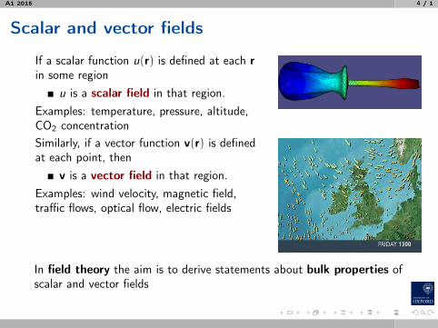
Scalar and vector fields

If a scalar function u(r) is defined at each rin some region

u is a scalar field in that region.Examples: temperature, pressure, altitude,CO2 concentrationSimilarly, if a vector function v(r) is definedat each point, then

v is a vector field in that region.Examples: wind velocity, magnetic field,traffic flows, optical flow, electric fields

In field theory the aim is to derive statements about bulk properties ofscalar and vector fields

A1 2015 5 / 1

Line integrals through fieldsLine integrals are concerned with measuring

the integrated interaction with a field as you move through it onsome defined path.

Eg, given a map showingthe pollution density fieldin Oxford, how muchgunk would you breath inwhen cycling from collegeto the Department ondifferent routes?

Miasma

Vapours Stench

A1 2015 6 / 1

Not entirely frivolous ...

NO2 in area of SE London

2003 2010

A1 2015 7 / 1

Vector line integrals

1) Chop path L into vector segments δri .2) Multiply each segment by the field value atthat point in space.3) Sum products.Three types:

r

F(r)

δr

1: Integrand U(r) is a scalarfield. Integral is a vector.

I =∫LU(r)dr

2: Integrand a(r) is a vectorfield dotted with dr. Integral is ascalar:

I =∫La(r) · dr

3: Integrand a(r) is a vectorfield crossed with dr. Integral isvector.

I =∫La(r)× dr

A1 2015 8 / 1

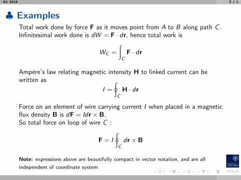
♣ ExamplesTotal work done by force F as it moves point from A to B along path C .Infinitesimal work done is dW = F · dr, hence total work is

WC =

∫CF · dr

Ampère’s law relating magnetic intensity H to linked current can bewritten as

I =∮CH · dr

Force on an element of wire carrying current I when placed in a magneticflux density B is dF = Idr × B.So total force on loop of wire C :

F = I∮C

dr × B

Note: expressions above are beautifully compact in vector notation, and are allindependent of coordinate system

A1 2015 9 / 1

♣ Examples

Q: A force F = x2y ı+ xy2 acts on a body at it moves between (0, 0)and (1, 1). Find work done when the path is:

1 along the line y = x .2 along the curve y = xn.3 along the x axis to the point

(1, 0) and then along the linex = 1

0,0 0,1

1,1

1

2 3

A:In planar Cartesians r = ıx + y ⇒dr = ıdx + dyThen the work done is∫

LF · dr =

∫L(x2y ı+ xy2 ) · (ıdx + dy) =

∫L(x2ydx + xy2dy) .

A1 2015 10 / 1

Example Path 1

PATH 1: For the path y = x we find thatdy = dx . So it is easiest to convert all yreferences to x .

0,0 0,1

1,1

1

2 3

∫ (1,1)(0,0)

(x2ydx + xy2dy) =

∫ x=1

x=0(x2xdx + xx2dx)

=

∫ x=1

x=02x3dx

=[x4/2

∣∣x=1x=0 = 1/2 .

NB! Although x , y involved these are NOT double integrals.Why not?

A1 2015 11 / 1

Example Path 2

0,0 0,1

1,1

1

2 3

PATH 2: For path y = xn

dy = nxn−1dx

Again convert y references to x .

∫ (1,1)(0,0)

(x2ydx + xy2dy) =

∫ x=1

x=0(xn+2dx + nxn−1.x .x2ndx)

=

∫ x=1

x=0(xn+2dx + nx3ndx)

=1

n + 3+

n3n + 1

A1 2015 12 / 1

Example Path 3

0,0 0,1

1,1

1

2 3

PATH 3: not smooth, so break into two.Along the first section, y = 0 and dy = 0,along second section x = 1 and dx = 0:

∫B

A(x2ydx + xy2dy) =

∫ x=1

x=0(x20dx) +

∫ y=1

y=01.y2dy

= 0+[y3/3

∣∣y=1y=0

= 1/3 .

Line integral depends on path taken

A1 2015 13 / 1

♣ Example 2

Q2: Repeat path (2), but now using the Force F = xy 2ı+ x2y .A2:

F · (ıdx + dy) = xy2 dx + x2y dy .

For the path y = xn we find that dy = nxn−1dx , so∫ (1,1)(0,0)

(xy2dx + x2ydy) =

∫ x=1

x=0(x2n+1dx + nxn−1x2xndx)

=

∫ x=1

x=0(x2n+1dx + nx2n+1dx)

=1

2n + 2+

n2n + 2

=12

This is independent of n, soThis line is independent of path!

Can we understand why?

A1 2015 14 / 1

Line integrals in Conservative fieldsWrite

g(x , y) = x2y2/2

Then the perfect differential is

dg =∂g∂x

dx +∂g∂y

dy = y2xdx + x2ydy

So our line integral∫F · dr =

∫B

A(y2xdx + yx2dy) =

∫B

Adg = gB − gA

It depends solely on the value of g at the start and end points, and notat all on the path

A vector field which gives rise to line integrals which are independent ofpaths is called a conservative field

A1 2015 15 / 1

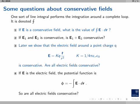
Some questions about conservative fieldsOne sort of line integral performs the integration around a complete loop.It is denoted

∮1 If E is a conservative field, what is the value of

∮E · dr ?

2 If E1 and E2 is conservative, is E1 + E2 conservative?

3 Later we show that the electric field around a point charge q

E = Kqrr2 K = 1/4πεrε0

is conservative. Are all electric fields conservative?

4 If E is the electric field, the potential function is

φ = −

∫E · dr .

So are all electric fields conservative?

A1 2015 16 / 1

Line integrals & parametrized curves

♣ Example 1:Q: Evaluate

∫F · dr when F = z ı+ y2 + xy k from (0, 0, 0) to (1, 1, 1)

along the space curve x = p, y = p2, z = p3.A:

F = p3ı+ p4 + p3kdr = dx ı+ dy + dz k

= dpı+ 2pdp+ 3p2dpk∫F · dr =

∫p=1

p=0(p3dp + 2p5dp + 3p5dp)

=[(1/4)p4 + (5/6)p6

∣∣p=1p=0

= (26/24) .

Suppose the integral was from (0, 0, 0) to (−2, 4,−8) ...∫p=?

p=?

A1 2015 17 / 1

Line integrals & parametrized curves /ctdAbove,

∫F · dr boiled down to working out some straightforward∫

F (p)dp. So, while the following don’t appear to involve vectors, theycould be the last stage in a vector integral ...

♣ 2:Consider

I =∫LF (x , y , z)ds ,

where the path L is the curve defined as x = x(p), y = y(p), z = z(p).First, convert the function to F (p), writing

I =∫pend

pstart

F (p)dsdp

dp

where (from Lec 3)dsdp

=

[(dxdp

)2

+

(dydp

)2

+

(dzdp

)2]1/2

.

Then do the (now straightforward) integral w.r.t. p.

A1 2015 18 / 1

Line integrals & parametrized curves /ctd

I =∫LF (x , y , z)ds

♣ 3: Suppose parameter is arc-length s andthe path L is x = x(s), y = y(s), z = z(s).Convert the function to F (s), writing

I =∫ send

sstartF (s) ds

♣ 4: If p is x — so y = y(x) and z = z(x) (or similar for p = y or p = z)

I =∫ xend

xstart

F (x)

[1+

(dydx

)2

+

(dzdx

)2]1/2

dx .

A1 2015 19 / 1

Surface integrals

Surface S is divided into infinitesimal vectorelements of area dS:

the dirn of the vector dS is the surfacenormalits magnitude represents the area ofthe element.

dS

Again there are three possibilities:1:

∫S UdS — scalar field U;

vector integral.2:

∫S a · dS — vector field a;

scalar integral.

3:∫

S a× dS — vector field a;vector integral.

A1 2015 20 / 1

Physical example of surface integral

Physical examples of surface integralsoften involve the idea of flux of a vectorfield through a surface∫

Sa · dS

Mass of fluid crossing a surface elementdS at r in time dt is

dM = ρ v · dSdt

Total rate of gain of mass can beexpressed as a surface integral:

dMdt

=

∫Sρ(r)v(r) · dS

dSa

Note that expression is free of any coordinate system

A1 2015 21 / 1

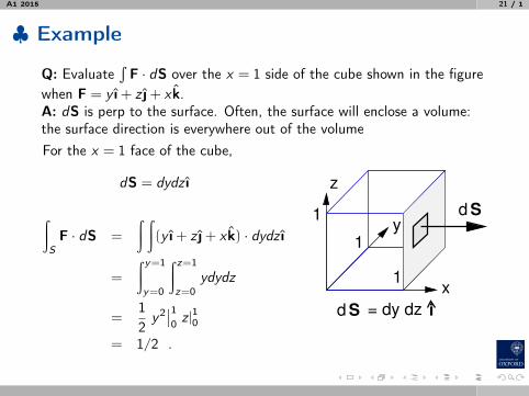
♣ Example

Q: Evaluate∫F · dS over the x = 1 side of the cube shown in the figure

when F = y ı+ z + x k.A: dS is perp to the surface. Often, the surface will enclose a volume:the surface direction is everywhere out of the volumeFor the x = 1 face of the cube,

dS = dydz ı

∫SF · dS =

∫ ∫(y ı+ z + x k) · dydz ı

=

∫ y=1

y=0

∫ z=1

z=0ydydz

=12

y2∣∣10 z |10

= 1/2 .

1

1

x

z

y

1

dS

dS = dy dz i

A1 2015 22 / 1

Volume integrals

The definition of the volume integral is again taken as the limit of a sumof products as the size of the volume element tends to zero.

One obvious difference though is that the element of volume is a scalar.

The possibilities are:

1:∫

V U(r)dV — scalar field; scalar integral (1P1 stuff!)

2:∫

V a(r)dV — vector field; vector integral. In this case one can treateach component separately.∫

VadV =

∫V

a1(x , y , z )ıdV +

∫V

a2(x , y , z )dV +

∫V

a3(x , y , z)kdV

= ı∫V

a1(x , y , z)dV + ∫V

a2(x , y , z)dV + k∫V

a3(x , y , z)dV

So, 3× 1P1 stuff.

A1 2015 23 / 1

Changing variables: curvilinear coordinates

Before dealing with further examples of line, surface and volume integralsit is important to understand how to convert an integral from one set ofcoordinates into another

You saw how to do this for scalar volume integrals in 1P1 (and we’veseen that volume integrals can always be handled as scalars)

— but we need to understand where Jacobians came from, and how wecan apply the mechanism more generally.

You will find the general problem slightly heavy going

— the better news is that later we specialize to the standard set of polarcoordinate systems

A1 2015 24 / 1

Changing variables: curvilinear coordinatesThe line integral in Cartesian coordinates uses

r = x ı+ y + z k and dr = dx ı+ dy + dz k

You can be sure that length scales are properly handled because|dr| = ds =

√dx2 + dy2 + dz2.

But often symmetry screams at you to change coordinate system:

likely to be plane, cylindrical, or spherical polars,but can be something more general like “u, v ,w ”— a curvilinear coordinate system

Now the bad news: Length scales are screwed upr 6= uu+ v v + ww

dr 6= duu+ dv v + dww

|dr| = ds 6=√

du2 + dv2 + dw2 .

A1 2015 25 / 1

Finding the length scalesConsider the transform to u, v where x = x(u, v) and y = y(u, v)

We writer = x(u, v )ı+ y(u, v )

And because

dx =∂x∂u

du +∂x∂v

dv

dy =∂y∂u

du +∂y∂v

dv

lines of constant x

lines o

f consta

nt y

yy

x x

lines of constant vlines of const u

we can write dr =

(∂x∂u

du +∂x∂v

dv)ı+(∂y∂u

du +∂y∂v

dv)

=

(∂x∂u

ı+∂y∂u

)

du +

(∂x∂v

ı+∂y∂v

)

dv

= hu u du + hv v dv

hu and hv are called metric coefficients

A1 2015 26 / 1

Metric coefficients, ctdTo repeat, the metric coefficients appear in

dr =

(∂x∂u

ı+∂y∂u

)

du +

(∂x∂v

ı+∂y∂v

)

dv

= hu u du + hv v dv

hu,v are the factors that turn the du, dv , or whatever, into proper lengths.But we can also write

dr =∂r∂u

du +∂r∂v

dv ⇒huu =∂r∂u

& hv v =∂r∂v

As u has to be a unit vector, we find that

hu =

∣∣∣∣∂r∂u

∣∣∣∣ =[(∂x∂u

)2

+

(∂y∂u

)2]1/2

and similarly for v

A1 2015 27 / 1

We can tie this in with tangentsIf we write the position vector as

r = x(u, v )ı+ y(u, v )

we find the tangent to a v -constantcurve as

∂r∂u

=∂x∂u

ı+∂y∂u

z

y

x

lines of constant vlin

es o

f consta

nt u

(∂r

∂u

)du

(∂r

∂v

)dv

* This is like dr/dp but is partial because there are two parametersand v is being held constant!

But u is not arclength, so ∂r/∂u will not be a unit tangent, rather

∂r∂u

= huu , so hu =

∣∣∣∣∂r∂u

∣∣∣∣ & u =1hu

∂r∂u

and similarly for v. Exactly what we derived before!

A1 2015 28 / 1

To summarize ...

These ideas extend to n-vectors without need for further proof.

Summary

r = x(u, v ,w )ı+ y(u, v ,w )+ z(u, v ,w)k

dr = huduu + hvdv v + hwdww

hu =

∣∣∣∣∂r∂u

∣∣∣∣ hv =

∣∣∣∣∂r∂v

∣∣∣∣ hw =

∣∣∣∣∂r∂w

∣∣∣∣∣∣∣∣∂r∂u

∣∣∣∣ =[(∂x∂u

)2

+

(∂y∂u

)2

+

(∂z∂u

)2]1/2

and similarly for others.

A1 2015 29 / 1

Surface integrals and curvilinear coordinates

The surface element is a vector productdSi = (dy )× (dz k)

In curvi coordsdSw 6= (duu)× (dv v)

Locally the surface element is planar, so

dSw =∂r∂u

du × ∂r∂v

dv

= huduu× hvdv v z

y

x

lines of constant vlin

es o

f consta

nt u

(∂r

∂u

)du

(∂r

∂v

)dv

The general 3D result for dSw in (u, v ,w) coords is

dSw = huhvdudv(u× v)

For an orthogonal curvilinear coord system, u× v = w and

dSw = huhvdudvw

A1 2015 30 / 1

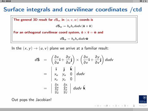
Surface integrals and curvilinear coordinates /ctd

The general 3D result for dSw in (u, v ,w) coords is

dSw = huhvdudv(u × v)

For an orthogonal curvilinear coord system, u × v = w and

dSw = huhvdudvw

In the (x , y)→ (u, v) plane we arrive at a familiar result:

dS =

(∂x∂u

ı+∂y∂u

)×(∂x∂v

ı+∂y∂v

)

dudv

=

∣∣∣∣∣∣

ı kxu yu 0xv yv 0

∣∣∣∣∣∣dudv

=

∣∣∣∣∂x∂u

∂x∂v

∂y∂u

∂y∂v

∣∣∣∣ dudv k

Out pops the Jacobian!

A1 2015 31 / 1

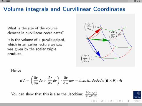
Volume integrals and Curvilinear Coordinates

What is the size of the volumeelement in curvilinear coordinates?

It is the volume of a parallelopiped,which in an earlier lecture we sawwas given by the scalar tripleproduct. (

∂r

∂u

)du

(∂r

∂v

)dv

(∂r

∂w

)dw

Hence

dV =

(∂r∂u

du × ∂r∂v

dv)· ∂r∂w

dw = huhvhwdudvdw(u× v) · w

You can show that this is also the Jacobian: ∂(x ,y ,z)∂(u,v ,w)

A1 2015 32 / 1

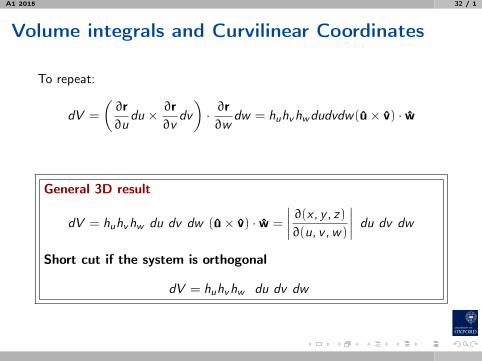
Volume integrals and Curvilinear Coordinates

To repeat:

dV =

(∂r∂u

du × ∂r∂v

dv)· ∂r∂w

dw = huhvhwdudvdw(u× v) · w

General 3D result

dV = huhvhw du dv dw (u× v) · w =

∣∣∣∣∂(x , y , z)∂(u, v ,w)

∣∣∣∣ du dv dw

Short cut if the system is orthogonal

dV = huhvhw du dv dw

A1 2015 33 / 1

The Polars

Some curvilinear coordinate systems are orthogonal, meaning that u, vand w are mutually perpendicular, so that

u× v = w and (u× v) · w = 1

We look atplane polarscylindrical polarsspherical polars

A1 2015 34 / 1

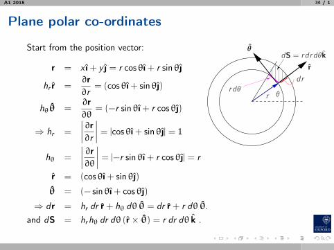
Plane polar co-ordinates

Start from the position vector:

r = x ı+ y = r cos θı+ r sin θ

hr r =∂r∂r

= (cos θı+ sin θ)

hθθ =∂r∂θ

= (−r sin θı+ r cos θ)

⇒ hr =

∣∣∣∣∂r∂r

∣∣∣∣ = |cos θı+ sin θ| = 1

hθ =

∣∣∣∣∂r∂θ

∣∣∣∣ = |−r sin θı+ r cos θ| = r

r = (cos θı+ sin θ)

θ = (− sin θı+ cos θ)

⇒ dr = hr dr r + hθ dθ θ = dr r + r dθ θ.and dS = hrhθ dr dθ (r × θ) = r dr dθ k .

dS = rdrdθkθ

r

r θ

dr

rdθ

A1 2015 35 / 1

Cylindrical polar coordinates

x

y

z

zφ

rP

R

ı

k

r

φ

r

y

z

x

Lines of

constant φ

Lines of

constant r

Lines of

constant z

x = r cosφ , y = r sinφ , z = z

Position vector R = x ı+ y + z k = r cos φı+ r sinφ+ z k

Why change the notation of position vector from r to R?If we did not, r would not equal |r|, and r would not be in same dirn as r.This could be confusing.

A1 2015 36 / 1

Cylindrical polars /ctd

R = r cos φı+ r sinφ+ z khr r = ∂R/∂r = (cos φı+ sinφ)

hφφ = ∂R/∂φ = (−r sin φı+ r cosφ)

hz z = ∂R/∂z = k⇒ hr = 1 and r = cos φı+ sinφ

hφ = r and φ = − sin φı+ cosφ

hz = 1 and z = k⇒ dR = dr r + rdφ φ+ dz z

and dSr = hφhzdφdz(φ× z) = r dφ dz r

dSφ = hzhrdzdr(z× r) = dz dr φdSz = hrhφdrdφ(r × z) = rdrdφzdV = r dr dφ dz

A1 2015 37 / 1

♣ Example: Line integral in cylindrical polarsFrom the list: change in position vector is dR = dr r + rdφ φ+ dz z

Q: Evaluate∮

C a · dR, where a = x3 − y 3ı+ x2y k and C is the circle ofradius ρ in the z = 0 plane, centred on the origin.

A: Turn a into cp’sa = ρ3(− sin3 φı+ cos3φ+ cos2φ sinφk)Since dz = dr = 0 on our particular path,and the constant r = ρ,

dR = ρ dφ φ = ρdφ(− sin φı+ cosφ)

so that∮Ca·dR =

∫2π

0ρ4(sin4φ+cos4φ)dφ =

3π2ρ4 x

y

z

rφ

d l = rdφφ

NB! For line integrals you will often see the element along the pathwritten as d` (or dr). Just roll with it ...

A1 2015 38 / 1

Surface integrals in cylindrical polars

Reminder ...

x

y

z

dz z

dz z

dr r

dr rrdφφ

rdφφ

dSz = rdrdφz

dSr = rdφdz r

dSφ = drdz φ

Cylindrical polars:Often-used surface area elementsare:

dSz = dr r × rdφφ = r dr dφ zdSr = rdφφ× dz z = r dφ dz r

Less often needed is

dSφ = hzhrdzdr(z× r) = dz dr φ

A1 2015 39 / 1

♣ Example: Surface integral in cyl polarsQ: Find

∫S v · dS when v = y 2ı+ x2 and the surface S is a cylinder of

radius a and height h whose base sits on the x , y plane and whose axiscoincides with k.

A: v has zero k component, so there is no contribution from the top(where dS = +r dr dφk) or bottom (dS = −r dr dφk).From the wall of the cylinder∫

v · dS =

∫h

z=0

∫2π

φ=0(a2 sin2 φı+ a2 cos2φ) · (a dφ dz r)

But r = cos φı+ sinφ, so∫v · dS = a3

∫h

z=0

∫2π

φ=0(sin2φ cosφ+ cos2φ sinφ)dφ dz

=a3h3[sin3φ− cos3φ)

]2π0 = 0

Can we see why zero? ....

A1 2015 40 / 1

Surface integrals in cylindrical polars

... plot the vector field v = y 2ı+ x2 from above. The red ring is thecylinder.

−1 −0.5 0 0.5 1

−1

−0.8

−0.6

−0.4

−0.2

0

0.2

0.4

0.6

0.8

1

As much v flows in as flows out, and∫v · dS is the net outflow or efflux.

A1 2015 41 / 1

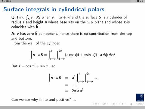
Surface integrals in cylindrical polarsQ: Find

∫S v · dS when v = x ı+ y and the surface S is a cylinder of

radius a and height h whose base sits on the x , y plane and whose axiscoincides with k.

A: v has zero k component, hence there is no contribution from the topand bottom.From the wall of the cylinder∫

v · dS =

∫h

z=0

∫2π

φ=0(a cos φı+ a sinφ) · a dφ dz r

But r = cos φı+ sinφ, so∫v · dS = a2

∫h

z=0

∫2π

φ=0...

= ....

= 2π h a2

Can we see why finite and positive? ...

A1 2015 42 / 1

Surface integrals in cylindrical polars

... plot the vector field v = x ı+ y . The red ring is the cylinder ...

−1.5 −1 −0.5 0 0.5 1 1.5

−1

−0.5

0

0.5

1

∫v · dS is the net efflux — clearly positive

A1 2015 43 / 1

Volume integrals in cylindrical polars

x

y

z

dV = dxdydzdx ı

dy

dz k

x

y

z

φ

dφrdφ

dz z

dr r

rdφφ

dV = rdrdφdz

In Cartesians, volume element given by

dV = dx ı · (dy × dz k) = dx dy dz

In cylindrical polars, volume element given by

dV = dr r · (rdφφ× dz z) = r dφ dr dz

NB: Volume is scalar triple product, hence:

dV =

∣∣∣∣∣∣

rdrφrdφzdz

∣∣∣∣∣∣=

∣∣∣∣∣∣∣

∂x∂r

∂y∂r

∂z∂r

∂x∂φ

∂y∂φ

∂z∂φ

∂x∂z

∂y∂z

∂z∂z

∣∣∣∣∣∣∣dr dφ dz

A1 2015 44 / 1

Spherical polars

x

y

z

ı

k θφ

r

P

r

φ

θ

x

y

z

Lines of constant

Lines ofconstant r

Lines of constant

φ

θ

(longitude)

(latitude)

Can use r again ...

x = r sin θ cosφ , y = r sin θ sinφ , z = r cos θr = x ı+ y + z k

= r sin θ cos φı+ r sin θ sinφ+ r cos θk

A1 2015 45 / 1

Spherical polars /ctd

r = r sin θ cos φı+ r sin θ sinφ+ r cos θk⇒ hr r = ∂r/∂r =

hθθ = ∂r/∂θ =

hφφ = ∂r/∂φ =

⇒ hr = 1 , hθ = r sin θ, hφ = r

⇒ r = sin θ cos φı+ sin θ sinφ+ cos θkθ = cos θ cos φı+ cos θ sinφ− sin θkφ = − sin θı+ cosφ

⇒ dr = dr r + rdθ θ+ r sin θ dφ φdSr = r2 sin θ dθ dφ r on spherical surface

dSθ = ? dr dθ θ on conical surface: DIY

dSφ = r dr dφ φ on planar hemisphere surfacedV = r2 sin θ dr dθ dφ

A1 2015 46 / 1

Surface integrals in spherical polars

Three possibilities, but most useful are surfaces of constant rThe surface element dSr is given by

dSr = hθdθθ× hφdφφ= r2 sin θdθdφr

x

y

z

rdθθ

r sin θdφφ

dSr = r2 sin θdθdφr

A1 2015 47 / 1

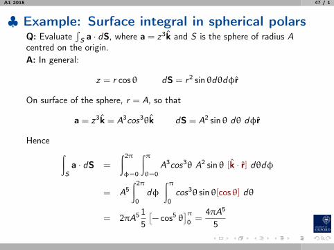
♣ Example: Surface integral in spherical polarsQ: Evaluate

∫S a · dS, where a = z3k and S is the sphere of radius A

centred on the origin.A: In general:

z = r cos θ dS = r2 sin θdθdφr

On surface of the sphere, r = A, so that

a = z3k = A3cos3θk dS = A2 sin θ dθ dφr

Hence ∫Sa · dS =

∫2π

φ=0

∫πθ=0

A3cos3θ A2 sin θ [k · r] dθdφ

= A5∫2π

0dφ

∫π0

cos3θ sin θ[cos θ] dθ

= 2πA5 15[− cos5 θ

]π0 =

4πA5

5

A1 2015 48 / 1

Volume integrals in spherical polars

x

y

z

rdθθ

r sin θdφφ

dr r

dV = r2 sin θdrdθdφ

dφ

dφ

dθ

θ

φ

r

r sin θdφ

r sin θ

Volume element given by

dV = dr r.(rdθθ× r sin θdφφ) = r2 sin θdrdθdφ

Note again that this volume could be written as a determinant

A1 2015 49 / 1

Summary

We introduced line, surface and volume integrals involving vectorfields.

We defined curvilinear coordinates, and realized that metriccoefficient were necessary to relate change in an arbitrary coordinateto a length scale.

We showed in detail how line, surface and volume elements arederived, and how the results specialized for orthogonal curvilinearsystem, in particular plane, cylindrical and spherical polarcoordinates.

Working stuff out from first principles has been hard going: as theexamples showed, application is much easier!