A wavelet transform coder supporting browsing and transmission of sea ice SAR imagery

2464 IEEE TRANSACTIONS ON GEOSCIENCE AND REMOTE SENSING, VOL. 40, NO. 11, NOVEMBER 2002

A Wavelet Transform Coder Supporting Browsingand Transmission of Sea Ice SAR Imagery

Juha Karvonen and Markku Similä

Abstract—A wavelet-transform-based algorithm for sea ice syn-thetic aperture radar (SAR) image data compression is presented.Compression of the relatively low resolution (100 m) SAR datais necessary to enable the transmission of such images from theFinnish Ice Service to users in the Baltic Sea. On board the ships,the SAR images are used for navigation purposes. Hence, in the vi-sual appearance of the compressed image, special attention must bepaid to the sharpness of small details. Several target-dependent fea-tures are incorporated in the compression scheme developed here.The addition of these features was motivated by an examinationof the wavelet coefficient statistics for the SAR data. In the quan-tization phase, the sensitivity characteristics of the human visualsystem were taken into account. As a result, the proposed algorithmdeviates in several respects from the standard procedures used inwavelet-based compression. The algorithm requires the setting upof multiple user-defined parameters to satisfy the requirements ofthe users and data. This requires supervision of an expert, but alsomakes it flexible for many kinds of data and user requirements.The algorithm presented here gives satisfactory results with a com-pression ratio of 20:1. Since only the location of ice-covered areasis of significance for ship traffic, the algorithm introduced containsan option to mask off open sea areas with the aid of an automaticopen-water detection procedure. We also report the results of auser evaluation, in which the proposed algorithm is compared tothe algorithm currently used by the Finnish Ice Service, as well asto the JPEG standard. The results of the evaluation favor the useof the proposed algorithm.

Index Terms—Image compression, sea ice, synthetic apertureradar (SAR), wavelets.

I. INTRODUCTION

I MAGE COMPRESSION is a widely researched area today.This is because of the requirements for transmitting high-

precision images and video (through wired (i.e., Internet) andwireless networks) and efficient storage. However, most of thisresearch is concentrated on optical images and video. The re-search of remote sensing data compression, especially the com-pression of detected SAR imagery over a specific target,is doc-umented later. The number of operative users of SAR data whogain from the compression of these expensive data is still rel-atively small. High-resolution SAR images can be very large,and efficient compression of the data is, therefore, importantfor transmitting the data to roaming users or for data storage. Inthis paper, we introduce a synthetic aperture radar (SAR) com-pression algorithm that currently is under test by the Finnish IceService (FIS).

Manuscript received February 7, 2002; revised July 12, 2002. The project wassupported by Tekes, the Finnish Technology Agency.

The authors are with the Finnish Institute of Marine Research, 00931Helsinki, Finland (e-mail: [email protected] or [email protected]).

Digital Object Identifier 10.1109/TGRS.2002.805068

The task of the FIS, an operational unit of the Finnish Instituteof Marine Research (FIMR), is to monitor ice conditions in theBaltic Sea, a brackish water area with seasonal ice cover. Thesea ice cover is relatively thin (with a mean thickness of usu-ally less than 70 cm). However, the deformed ice fields exhibita large variability in their degree of difficulty for marine navi-gation. Knowledge of local ice conditions is of utmost impor-tance for merchant vessels and ice breakers. FIS prepares dailya varied set of sea ice information products about the ice situ-ation to fulfil the needs of its customers. C-band RADARSATScanSAR Narrow images, with a coverage of 300 km300 kmand original spatial resolution of 50 m, constitute an essentialinformation source in the operational sea ice monitoring. TheRADARSAT images are received , processed, and compressedusing the Lempel–Ziv algorithm [1] by the Tromsö Satellite Sta-tion (TSS). They are then transferred to the FIS via the Internet.After further processing at FIS (Section II-A), a whole SARscene or a part of it is transmitted to vessels for visual assess-ment at a resolution of 100 m. At best, a SAR image is receivedonboard a few hours after the overflight of the satellite.

Due to the narrow bandwidth in use (the Global Systemfor Mobile Communications (GSM) network widely in usein Scandinavia) and the huge size of the images (typically6–10 MB), the data require strong compression. Currently,this is solved by using downsampling and adaptive Laplacianpyramid (ALP) coding [2], [3] of the downsampled images. Inthis paper, a wavelet-based algorithm (named SARKOMP, anacronym for “SAR compression” in Finnish) is introduced toreplace the ALP algorithm in operational use. When designingthe SARKOMP algorithm, our aim has been to take intoaccount explicitly some characteristic features of the availablesea ice SAR image data, e.g., the geometry of the edges presentin images. The design of a compression scheme is governed bythe application of the compressed image. Since these imagesare used onboard a ship to infer the current ice conditions, thecompression must preserve the amount and sharpness of thesmall details present in the image as well as possible.

A most comprehensive attempt to model the backscatteringfrom the Baltic Sea ice is made in [4]. There the model compu-tations indicated that the single most important factor causinglocal fluctuation in the backscattering found in C-band SAR im-ages over the Baltic sea is the variation in the ice surface rough-ness. The largest changes in the ice surface roughness are cre-ated by the occurrence of ice ridges. These are thick, long, andnarrow accumulations of ice blocks with a typical sail heightless than 2 m in the Baltic Sea. The width of an ice ridge varieswidely, but usually has a magnitude of a few meters. Also, thedensity of the occurrence of ice ridges has a large spatial varia-

0196-2892/02$17.00 © 2002 IEEE

KARVONEN AND SIMILÄ: WAVELET TRANSFORM CODER 2465

tion [5]. From the point of view of navigation, the most impor-tant tasks are to discriminate between open water and ice-cov-ered areas and to detect highly deformed ice areas using a SARscene. The major texture elements in a sea ice SAR image arethe edges, which indicate either a ridge, a ship track, an ice floeedge, or a transition from highly deformed ice area (like a rubblefield or strongly ridged area) to a smoother ice surface.

The ridged ice areas often have a blurred appearance in a SARimage, and their visual assessment is difficult, even from theoriginal data. There are two major reasons for the blur. First, thediffuse scattering usually dominates, because the scatterers withthe strongest returns, i.e., ice ridges and the resolution (100 m) atwhich this scattering process is observed, have a fundamentallydifferent spatial scale. Secondly, the magnitude of roughness at ascale comparable to the radar wavelength influences the averagebackscattering level and, thereby, the contrast between level iceand ridged ice areas [6]. As a result, many of the edges present inour images are quite fragmented in nature and, in addition, ofteninvolve only weak contrast with respect to the background. Theweakness of the contrast can be partially attributed to the loga-rithmic scaling applied to our SAR data (Section II). Actually,we have taken the restoration of edges as one of the propertiesagainst which the different compression schemes are assessed(Section VI-B).

Wavelet transform has been applied with great success tonumerous image compression problems (see [7]). However,in connection with detected SAR imagery, only relativelyfew compression articles utilizing the transform coding haveappeared. Some recent contributions are [8]–[11]. Baxter [10]used the Gabor transform and utilized in his work resultsrelated to the human visual system (HVS) processing. Also, inour approach, observations made in the analysis of the HVSare employed, although differently than in [10]. The paper byZeng and Cumming [11] appeared during revision of our paper.Their approach relies on the tree-structured wavelet transform,which is closely related to wavelet packet decomposition.Some ideas similar to our approach are presented in [11], e.g.,a homogeneous set (here “textureless area”) and a target set(here “textured area”). Unfortunately, the approach in [11] alsocontains several adjustable parameters just like ours. A variantof the Fourier transform, i.e., a discrete cosine transform overthe blocks, is implemented in the standard JPEG algorithm[12]. In Section VII-B, we will briefly discuss our experienceswith this transform coding method. We have also investigatedusing fractal coding for sea ice SAR images [13].

The wavelet transform yields for several image classes asparse representation in the context of coding of noise freedata [7]. In the wavelet transform coding, one is actually facedwith three major issues: the determination of the threshold(s)(a wavelet coefficient with a magnitude larger than the giventhreshold is retained), the quantization of the values of theretained coefficients, and an efficient coding of the location ofthe zeroes in the wavelet plane. In this paper, all these aspectswill be discussed. The problem of the speckle, which influ-ences fundamentally the SAR image statistics and makes thecompression such a complex issue, is discussed in connectionwith thresholding and of coding the location of zeroes in thewavelet plane.

The outline of the paper is as follows. Section II first reviewsthe main properties of the TSS-processed SAR images. Becauseour aim is to compress the areas with a weak texture more thanthe areas of strong textural variation, the textural variation isalso treated in this section. Section III describes the implemen-tation of the wavelet transform as well as the choice of a suitablebasis. In Section IV, different statistics of wavelet coefficientsare investigated. A detailed description of the implementationof the algorithm can be found in Section V. In this section, wealso show how results obtained from the sensitivity analysis ofthe HVS can be utilized during the quantization. In Section VI,some central design choices of the coder are justified throughstatistical analysis. Finally, in Section VII, some experimentalresults are presented. Also, the important option of maskingthe open sea and compressing only the ice-covered area is pre-sented. Section VIII contains the conclusions.

The usability of a compression scheme should be assessed inthe light of the particular application in which the algorithm isutilized. The presented algorithm is designed for sea ice SARimages. If the target of interest is an urban area or forests, mod-ifications for the algorithm are perhaps needed in order to re-trieve the most important features of the target. When in the fol-lowing we refer to SAR images, we always mean sea ice SARimages with a relatively low resolution (100 m). If the resolu-tion of the data is changed, our algorithm still applies, but theefficient thresholds must be determined anew. The user-definedparameters of the algorithm can be adjusted suitable to manykinds of datasets and user requirements. This adjusting needsto be made by an expert aware of the user requirements for thespecific data and application.

II. DATA

A. The TSS Radarsat Images

The RADARSAT images are received and processed bythe Tromsö Satellite Station. In this process, the originalbackscatter intensity data (16-bit) are quantized and mapped toeight-bit values by logarithmic scaling. The original (quantized)backscattering coefficients can be recovered from the deliveredRADARSAT images by using the equation (a communicationfrom TSS)

(1)

where is the pixel value in the SAR image (0–255);is the logarithmic scale; is the logarithmic gain

factor; and is the local incidence angle. The 8-bpp images re-ceived from TSS are geometrically rectified to ground projec-tion (Mercator) [14], and the land area is masked off. Duringthe rectification process, the pixel resolution is lowered fromthe original 50 m to 100 m.

We sometimes call the received SAR images “TSSRADARSAT images” to emphasize the fact that the ScanSARdata are processed at the Tromsö Satellite Station with theirown software. Discussion of the impact of the logarithmictransform to image statistics is postponed until the concept ofthe textural variation is defined.


Fig. 1. RADARSAT SAR scene that was used as a test image. The ice field iscomposed of old (brighter areas) and new ice (darker areas) with some deformedareas on the right side of the image (brightest areas). Also, several long and shortice ridges (narrow bright stripes) are visible in the scene. The resolution of thedata is 100 m.

B. The Test SAR Images

To examine the efficiency of the compression scheme, eighttest SAR scenes of size 512512 pixels were selected ran-domly from several RADARSAT ScanSAR Narrow images. Wechecked that the resulting test set was composed of images rep-resenting several kinds of ice conditions and that the SAR sceneswere acquired during cold conditions so that moisture would notreduce the dynamic range of scattering statistics. One of the testSAR scenes covered mainly open water without any strong fea-tures (test image 2). The results presented here were computedeither for one of the test SAR scenes (shown in Fig. 1) or for allthe test scenes. All these test SAR scenes are available from ourWeb page [15].

C. Texture in a SAR Image

The SAR data are very noisy. Hence, it is desirable that com-pression should be strongest in areas where the fluctuation ofthe pixel values can be considered to be caused mainly by thespeckle (a textureless area). On the other hand, more detailsshould be preserved in areas where one expects that the vari-ability of scattering statistics, due to the geometrical propertiesof the target, dominates the total signal oscillation at the finestscale (textured areas).

In order to perform this discrimination between texturelessand textured areas, we applied the concept of texture variancesuggested in [16] and utilized, for example, in [17] and [18].There the following multiplicative model was applied for di-viding the total within-field (pixel-to-pixel) variation betweentwo different fluctuation sources (the changing of the scattering

properties from pixel-to-pixel (texture variance) and the specklevariance)

(2)

where is the measured intensity of the pixel () repre-senting the field ; is the mean intensity over the same field;

is the texture random variable characteristic to the field withthe constraint ; and is the speckle random vari-able with a distribution accounting for the speckle of anintensity radar image with independent looks. The variable

is normalized to have . Then .In our application the word “field” refers to a relatively smallpatch of the ice surface that can be assumed to be statisticallyhomogeneous with respect to the most important ice parame-ters. Hence a “field” may be, for example, a level ice field or adeformed ice field with the same ridging intensity.

After some manipulation , one obtains ([16, p. 1911])

(3)

On the left-hand side of the equation is the variance to thesquared-mean ratio (VSMR). By employing (3), it is possible toassess the amount of variation attributed to the texture variance

when compared to the noise variance .The logarithmic transformation applied to the intensity SAR

values in the TSS SAR data converts the multiplicative specklenoise model to an additive noise model in which the specklenoise model can be approximated well by a Gaussian distribu-tion [19]; a precise speckle density determination after the loga-rithmic transformation is carried out in [20]. For a homogeneoustarget, the theory in [20] predicts that the standard deviation ofthe TSS pixel values is constant and depends only on the numberof looks used in the processing. In the mean value of the sig-nals scattered from a homogeneous target, the scaling introducesa bias dependent on. However, this bias is independent of thesignal level and is the same for all the homogeneous targets inthe scene [20].

To illustrate the effect of the logarithmic scaling, we com-puted the mean and the standard deviation over the open waterarea (extracted from test image 2) using pixel blocks of size16 16 pixels both for the intensity SAR image and the TSSSAR image. The open water area is visually featureless. Thestatistics for the open-water SAR intensity image are shown inFig. 2(a). The observed VSMR behavior in Fig. 2(a) supports theassumption that the variation in this SAR image is mainly due tospeckle. The same statistics for the same pixel blocks are shownfor the TSS SAR image in Fig. 2(b) where the speckle varia-tion remains at the same level independent of the mean radarreflectivity. For each TSS SAR image pixel block, the hypoth-esis about the Gaussian distribution was tested by computing thethird and fourth sample moments and by comparing them withtheir predicted Gaussian-distribution-based values. The fit wasvery good in almost all cases.

To evaluate the compression results, the texture variance isutilized in the following manner. The numberof looks presentin the TSS RADARSAT ScanSAR Narrow data is estimated tovary from to , depending on the incidence angle


(a)

(b)

Fig. 2. Here the SAR data consist of the same TSS RADARSAT imagetaken over open sea. In Fig. 2(a), the SAR data are converted to an intensitySAR image. In Fig. 2(b), the format of logarithmically scaled measurementrepresentation is used. In both figures, the blockwise standard deviations areplotted against the blockwise mean. The size of the block is 16� 16 pixels.

[21]. We did not compute the incidence angle for the selectedtest images. Hence we use 1/6 as a conservative estimate of thespeckle variance. We consider a pixel block as representing atextured area if the texture variance is greater than the givennoise variance, i.e., if . From Table V (dis-cussed in more detail in Section VI), one can see that large frac-tions of each test SAR images can be labeled as textured ac-cording to this criterion. The proportion of the textured areavaries from small (just 19.6% in test image 8 which consistsmainly of level ice) to large (the fraction may be about 90% intest images consisting of only drift ice).

III. W AVELET TRANSFORMIMPLEMENTATION

The orthogonal wavelet transform preserves energy. How-ever, a general shortcoming in using orthogonal compactly sup-

TABLE IWAVELET FILTERS USED IN THE ALGORITHM. H0 (LOW-PASS) AND G0

(HIGH-PASS) ARE THE ANALYSIS FILTERS. H1 (LOW-PASS) AND G1(HIGH-PASS) ARE THE SYNTHESIS FILTERS

ported real-valued wavelet filters for compression is that theyare all asymmetric except the Haar filter. This asymmetry blursedges during quantization, because asymmetric filters do notpreserve phase. Symmetric filters also make it easier to deal withthe boundaries of image [22, Ch. 8 and 10]. On the other hand,the biorthogonal wavelet filters can be symmetric, compactlysupported, and real-valued [22, Ch. 8]. In the biorthogonal case,the analysis filters (hereh0 andg0) differ from the synthesis fil-ters (hereh1 andg1). The wavelet functions associated with thefilters h1 andg1 are called the dual functions of the waveletfunctions associated with the filtersh0 andg0 (and vice-versa).The dual functions are orthogonal with respect to each other.

We used the 7/9 biorthogonal wavelet filters introduced in[23] and given in Table I. These filters are called Antoninifilters here. In addition to symmetry, the Antonini filters havealso other attractive properties. They are biorthogonal perfectreconstruction filters with the property that both the analysisand synthesis wavelets have the regularity of four vanishingmoments. Their dual functions are very similar. Hence, thebasis associated with the filters is almost orthogonal. Thequasi orthogonality guarantees that the they preserve almostenergy. The number of vanishing moments gives the filtersenough regularity to create small wavelet coefficients forslowly varying domains during the analysis phase, and also thereconstruction from the sparse data with quantized values isperformed smoothly [7, Ch. 7].

It is known that the Antonini filters perform well in thecompression of optical images [24]. To gain some insight intowhether the good performance of the Antonini filters is validalso for SAR imagery, we used the same kind of approach asin one of the tests performed in [24]. All the coefficients fromthe two finest scales were removed, and the image was recon-structed with the remaining coefficients. The reconstructionswere then assessed by visual inspection and according to thepeak-signal-to-noise ratio (PSNR) [for a definition see (22)].The following set of filters was included: Haar, Daubchechies,Symmlets, and Antonini (the coefficients for the first threefilter sets are given, for example, in [22]). The result was thatthe Antonini and the Symmlets with four vanishing moments


Fig. 3. Example of a two-level wavelet transform. (Upper left) Original image.(Upper right) Transform. (Lower left) Approximation image scaled up to theoriginal scale. (Lower right) Diagram showing how the image is divided infrequency space. If more levels are used in the wavelet transform, the LL-bandis (iteratively) divided further into four subchannels.

performed far better than the others. These filters preserved thesharpness of the edges and the small details in SAR imagerybest relative to the other tested filter sets according to bothvisual assessment and to the PSNR. One should note, however,that in all the reconstructions there were some visible artifactsdue to the large compression ratio. The Antonini filters werechosen because of their symmetry, which makes the utilizationof the interscale dependencies between the wavelet coefficientseasier (see Section VI-A).

The discrete wavelet transform is implemented by using sep-arable wavelet filters as described by, for example, Mallat [7].Hence, the two-dimensional convolution can be computed asone-dimensional (1-D) convolutions along the columns of theimage followed by 1-D convolutions along the rows

(4)

where the pair ( ) comprises high- and low-passfilters; variables and indicate the pixel coordinates; and

indicates the value of pixel in the location []. Theappropriate pairings of the filters in the analysis phase are(g0,h0), (h0,g0), (g0,g0), or (h0,h0). In the synthesis phase,one uses the corresponding pairings for the filtersh1 andg1.The pairing (g0,h0) refers to the fact that high-pass filtering isfirst applied along the columns, followed by low-pass filteringalong the rows. In Fig. 3, this operation is denoted by .Each filtering is followed by resampling by decimation (down-sampling) in the analysis phase and preceeded by upsamplingin the synthesis phase. The meaning of the other pairings andtheir corresponding abbreviations in Fig. 3 is obvious. In ouralgorithm we used five resolution levels.

IV. WAVELET STATISTICS OFSEA ICE SAR IMAGES

A. Statistics of TSS RADARSAT Images

The statistics of the discrete wavelet coefficients depend onthe noise type [see (4)]. The effect of the speckle on the mag-nitude of a coefficient is similar to the case of the standard de-viation (see Fig. 2), i.e., the local mean magnitude of waveletcoefficients (calculated from a pixel block) increases as a func-tion of the mean radar reflectivity for an intensity SAR imageand remains at the same level for a TSS RADARSAT image. Inthe computations, the same pixel blocks as for Fig. 2 were used.Due to the linearity of the transform, this behavior of waveletcoefficients is to be expected. Hence, if one wants to compressan intensity SAR image in the wavelet domain, some kind ofnormalization with respect to the mean radar reflectivity is nec-essary. One suggestion is to normalize by the value of the ap-proximation image in the wavelet decomposition [18].

We chose to work with the TSS RADARSAT pixel values.One benefit of this format is that we deal with a constant specklelevel. Another benefit is that we process the same data as theusers at sea inspect. This enables us to implement ideas origi-nating from the sensitivity analysis of the human visual system(see Section V-C).

B. Statistics of Frequency Distribution

We now consider some statistics describing the frequency dis-tribution of the wavelet coefficients. These statistics are entropy(which is directly proportional to the code length [25]) and kur-tosis. Kurtosis is defined as the normalized fourth moment ofthe random variable. The sample estimator of the kurtosis is (denotes the sample mean andthe sample standard deviation)

If the distribution is Gaussian, then . In the case ,the distribution is called sub-Gaussian (e.g., the uniform dis-tribution), and the case indicates super-Gaussian dis-tribution (e.g., the Laplacian distribution). This last case is im-portant in transform coding, since, if a new representation hasa super-Gaussian distribution, its distribution is more concen-trated around the mean value, and it has heavier tails than theGaussian distribution. From a compression point of view, this isdesirable because it implies that a significant part of the signalvariation is captured by a relatively few large coefficients. Ahigh kurtosis value also implies that most of the coefficients aresmall (the mean of the wavelet filter is zero) and can be removedfrom the recontruction without significant information loss.

In the following, we compare the statistics based on a singletest SAR scene (Fig. 1) with the corresponding quantities com-puted for the Lena image. These images are of the same size.Currently, a great deal of mathematical effort has been directedto understanding and characterizing the statistics of the photo-graphic data of natural scenes (like Lena) (for references into thecurrent state-of-the-art see, for example, [26]–[28]). Althoughthe comparison of a single SAR scene and a single photographicimage comprise only a case study, we hope that this comparisonilluminates the fundamental differences in the statistics of these


Fig. 4. Sample kurtosis of each detail image at the five finest scales is plottedfor the test SAR image and for the Lena image (three detail images per scale).The drawn horizontal line has a value 3 that is the kurtosis of the Gaussiandistribution.

two datasets. These comparisons also illustrate how the pres-ence of strong noise influences the statistics of the wavelet co-efficients. We would like to note that the results obtained fromthe other test SAR scenes (seven scenes) were qualitatively verysimilar.

The kurtosis values of the wavelet coefficients at the fivefinest scales (99.9% of all the coefficients) are displayed inFig. 4. We first note that the marginal distribution of the SARpixel values for the log case is almost a Gaussian one ( ).The wavelet transform enhances the non-Gaussian features indata. These features are related mostly to edges. At the finestscale, the frequency distribution of the coefficients and, hence,also the kurtosis value is close to a Gaussian distribution (

). One can suspect that at the finest scale most of the variationcan be attributed to fluctuations caused by the Gaussian noise.We recall that noise cannot be compressed. At the coarser res-olutions, the efficiency of the wavelet representation increases,and the kurtosis values vary between 4.5 and 7.3. For the othertest SAR images, the kurtosis behaves very much like it doesfor test image 4, being usually somewhat larger. Exceptions arethe test images with a very weak texture, i.e., images 2 (largeopen water area) and image 8 (mostly level ice). In these cases,the distributions remain at all resolutions close to the Gaussiancase, the kurtosis taking values between 3 and 4.

The efficiency of the wavelet basis is much better for a datasetlike the Lena image. In this image, the kurtosis increases from

for the original image to almost for some de-tail images at the two finest scales. The kurtosis statistics implythat the task of compressing an image can be carried out moreeffectively in the wavelet domain for Lena than for SAR im-agery because, unlike for SAR images, a reasonable approxi-mation even with a relatively few large wavelet coefficients forthe Lena image can be achieved.

Also, the entropies of the frequency distributions indicate thatthe compression of the Lena image is the easier one of these two

Fig. 5. Distribution of energy according to orientation at the four finestresolution levels (the test SAR and Lena images). The three detail images perscale appear in the order LH, HL, and HH. The total energy of the four finestscales is normalized to one.

images. The entropies are 4.5 bits per pixel (the number of uni-form quantization bins was 256) for the SAR scene and 2.0 bitsfor the Lena image. Hence, coding these coefficients with 256values for the SAR image, without any location information,would result in a code more than two times as long as for theLena scene.

C. Distribution of Energy

The orthogonal wavelet transforms preserve the energy (thesum of the squares of the pixel values) of the original image. Ac-tually, the energy equals the variance of a zero-centered image.The wavelet transform redistributes the variation present in theoriginal data according to the frequency and to the orientation.The biorthogonal distribution used here does not preserve theenergy exactly, but it is very stable due to its quasi orthogonality[7]. For our test images, the changes in the amount of the energywere maximally only a few percent of the total energy. In Figs. 5,6, and 8, we show the distribution of the energy in the waveletdomain from three different points of view.

Fig. 5 shows the energy of the three different detail imagesat the four finest scales. The energy present in a single detailimage is normalized by the total energy over the four finestscales. Probably the most fundamental feature in the distribu-tion of variation was that most of the energy in the SAR imageis concentrated in the two finest scales. This energy concentra-tion is in strong contrast to the respective results computed forthe Lena image, where the energy of a detail image increases asthe resolution level becomes coarser. On the basis of Fig. 5, itis evident that the smaller scale signal oscillation dominates thevisual appearance of the SAR image, unlike in the case of theLena image. Also, an important difference between the sea iceSAR image and the Lena image is that the energy of the SARimagery is distributed much more evenly between different de-tail images than in the Lena image where one detail image cor-responding to the vertical edges comprises most of the energy.

The distribution of the coefficients with the largest magnitudein the different detail images at the four finest scales is displayed


Fig. 6. Distribution of the largest wavelet coefficients according to orientationat the four finest resolution levels (the test SAR and Lena images). The threedetail images per scale appear in the order LH, HL, and HH. The frequency ofthe retained coefficients at the four finest scales is normalized to one.

in Fig. 6. Only the very largest coefficients (2.5%) were chosenbecause every compression strategy relying solely on the mag-nitude of the coefficient must include them. As shown in Fig. 6,most of the largest coefficients computed from the logarithmi-cally scaled SAR image can be found in the second finest scale.By combining the results presented in Figs. 4 and 5 with theresults of Fig. 6, one finds support for the assumption that theGaussian speckle variation accounts for most of the signal os-cillation detectable in the finest scale.

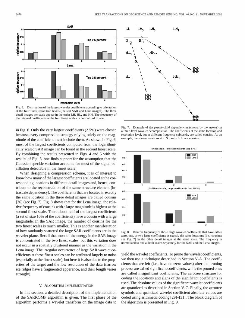
When designing a compression scheme, it is of interest toknow how many of the largest coefficients are located at the cor-responding locations in different detail images and, hence, con-tribute to the reconstruction of the same structure element (in-trascale dependency). The coefficients that are located in exactlythe same location in the three detail images are called cousins[26] (see Fig. 7). Fig. 8 shows that for the Lena image, the rela-tive frequency of cousins with a large magnitude is highest at thesecond finest scale. There about half of the largest coefficients(a set of size 10% of the coefficients) have a cousin with a largemagnitude. In the SAR image, the number of cousins for thetwo finest scales is much smaller. This is another manifestationof how randomly scattered the large SAR coefficients are in thewavelet plane. Recall that most of the energy in the SAR imageis concentrated in the two finest scales, but this variation doesnot occur in a spatially clustered manner as the variation in theLena image. The irregular occurrence of large SAR wavelet co-efficients at these finest scales can be attributed largely to noise(especially at the finest scale), but here it is also due to the prop-erties of the target and the low resolution of the data (narrowice ridges have a fragmented apperance, and their length variesstrongly).

V. ALGORITHM IMPLEMENTATION

In this section, a detailed description of the implementationof the SARKOMP algorithm is given. The first phase of thealgorithm performs a wavelet transform on the image data to

Fig. 7. Example of the parent–child dependencies (shown by the arrows) ina three-level wavelet decomposition. The coefficients at the same location andresolution level, but at different frequency subbands, are called cousins. As anexample, the shown locations atLH andHH are cousins.

Fig. 8. Relative frequency of those large wavelet coefficients that have eitherzero, one, or two large coefficients at exactly the same locations (i.e., cousins;see Fig. 7) in the other detail images at the same scale. The frequency isnormalized to one at both scales separately for the SAR and the Lena images.

yield the wavelet coefficients. To prune the wavelet coefficients,we then use a technique described in Section V-A. The coeffi-cients that are left (i.e., have nonzero values) after the pruningprocess are called significant coefficients, while the pruned onesare called insignificant coefficients. The zerotree structure forcoding the locations and signs of the significant coefficients isused. The absolute values of the significant wavelet coefficientsare quantized as described in Section V-C. Finally, the zerotreesymbols and quantized wavelet coefficient absolute values arecoded using arithmetic coding [29]–[31]. The block diagram ofthe algorithm is presented in Fig. 9.


Fig. 9. Block diagram of the algorithm.

We have adopted the zerotree structure and coding the ze-rotree labels from the embedded zerotree wavelet (EZW) algo-rithm [32]. Our algorithm uses the HVS-dependent quantizationthat is different from the successive approximation quantizationused in the EZW algorithm. We do not order the wavelet coef-ficients according to their importance as in EZW but take theirimportance to visual perception into account in our quantizationscheme. Thus, our algorithm also does not use embedding likeEZW. In the current operative application, the image is com-pressed with a suitable set of parameters and then transmitted toend-users either via satellite connection or mobile connection,depending on the receiver equipment onboard of the receivingvessel. After receiving the image, it is decompressed in the back-ground, and after that the user is notified about the arrival of anew image. The transmission protocol [33] handles the trans-mission errors. Progressive coding could be a useful addition tothe algorithm in the future, depending on the development of theoperative system.

There are multiple user-defined parameters, which need tobe set for a certain set of data (e.g., for a certain SAR instru-ment) and user requirements, in our algorithm. This usuallyneeds some expert supervision in the setup phase to adjust theparameters suitably. But it also gives a great flexibility for manydifferent kinds of datasets and user requirements. The parame-ters have now been adjusted for RADARSAT ScanSAR data. Afuture improvement would be to give more exact guidelines forselecting the parameters for different kinds of data.

A. Wavelet Coefficient Pruning

For the approximation image at level 5, we save all the coef-ficients. For the wavelet coefficients at resolution levels 3–5, athresholding is used that is dependent on the detail image sta-tistics, i.e., we prune coefficients whose absolute values are lessthan a threshold defined as

(5)

where the index refers to the detail image with standard devi-ation . The resolution-level-dependent factoris given as aparameter to the algorithm. The term takes into account thelocal statistics in the image by applying different thresholdingin different areas of the image. We were led to implement thisoption because of the change in local image statistics in the SARdata caused by change of incidence angle [21]. The amount ofthe local thresholding can be adjusted by a gain parameterasdescribed by the equation

(6)

A single threshold for all the coefficients is achieved by set-ting to zero, which is also the default value. Higher valuesthan zero cause the local variation to be taken into account pro-portionally to . The values of the factor are computed in thecenter of the local windows and smoothed between the differentwindows. The relative standard deviation at image lo-cation ( ) is computed as

(7)

where is the local standard deviation, andis the globalstandard deviation for the image. The local standard deviationis computed in an pixel window, where the value ofis a user-adjustable parameter.

At the two finest scales, we use a thresholding scheme thattakes into consideration whether the wavelet coefficient was de-termined as being significant at a previous scale (the interscaledependency). We first compute a threshold valueusing the sta-tistics for the second finest resolution level

(8)

We then divide the wavelet coefficients at level 2 into twocategories, i.e., the textured area coefficients and the texturelessarea coefficients. A coefficient is called a textured area coef-ficient (“cheaper” coefficient) if the wavelet coefficient at thenext lower resolution level at the same location is significant;otherwise, it is a textureless area coefficient (“expensive” coef-ficient). The thresholds applied to the textured area coefficientsand to the textureless area coefficients differ from each other.The different treatment of these areas is due to the zerotree al-gorithm as explained in Section VI-A.

The coefficient pruning process for the textured area coeffi-cients is as follows. First, we compute a threshold

(9)

where is as above and is a user-adjustable parameter. Thecondition for pruning is

otherwise(10)

where is the wavelet coefficient value, i.e., the coefficient ispruned if the absolute value is less than or equal to the threshold

. After applying the threshold , most of the significant co-efficients at resolution level 2 are determined. Let us denote theset of coefficients that satisfy the condition in (10) by A. In addi-tion to set A, some other coefficients (we denote the set of themhere by B) will also be included in the set of significant coeffi-cients. A coefficient will be included in set B if the coefficienttogether with the coefficients in A is believed to form an edgein the image. The stepwise procedure, described below, to de-termine if this is the case can be regarded as a geometric filter.

The test as to whether a coefficient is in the set B proceedsas follows. We first apply threshold to exclude very smallcoefficients from set B. Threshold is computed as

(11)

where is a user-adjustable parameter. Let us suppose thatthe magnitude of the coefficient exceeds this threshold. Thena 5 5 pixel neighborhood in the wavelet domain is studied


for coefficients for which the absolute strength, defined asthe sum of the coefficients’ absolute values in the three detailimages at the same resolution level (the sum of “cousins”; seeSection IV-C)

(12)

exceeds a third threshold value

(13)

where is a parameter. If in the 3 3 neighborhood there ismore than one coefficient, with the same sign as the coefficientstudied, whose absolute strengthexceeds and, additionally,if in the 5 5 neighborhood there is more than one coefficient,with the same sign as the coefficient tested and whose absolutestrength exceeds , then the coefficient is included in setB. The sign condition is necessary because, in the case ofsymmetric FIR filters, an edge pixel generates two largewavelet coefficients with different signs. A similar pruningprocess is performed for the textureless area coefficients butusing higher pruning factors , , and instead of , ,and (i.e., , , and ). All these valuesare user-adjustable parameters. At the finest resolution level, asimilar pruning process with textured and textureless areas isperformed.

We note that some interesting ideas for using the tree structurein the pruning or classification of the wavelet coefficients havebeen presented in [34].

B. Default Parameters

The current default parameters are presented in Table II. Forhigh compression ratios, the thresholds for the textureless areasat the finest resolution level were selected so large that no coeffi-cients in these areas are retained. The number of thresholds used(six thresholds for each of the two finest scales, one thresholdfor the resolution levels from 3–5) may detract from the factthat the algorithm is primarily controlled by the thresholds se-lected for the “cheap” ( ) and “expensive” ( ) co-efficients at the two finest scales. Reasonable values for thesethresholds can be determined for a particular image set by ex-amining the effects of different thresholding schemes using theconditional histograms as diagnostic tools as in Figs. 10 and 11.In order to gather representative information of the underlyingstatistics, the different thresholding schemes must be exploredfor several sample images.

The four remaining thresholds for the two finest scales can beselected then according to the principles given in Section V-A.From the coefficients at the three coarsest scales, only those rel-atively close to zero should be set to zero. Using small thresh-olds for these resolution levels yields much information for thereconstruction at small cost because the total amount of the co-efficients at these levels is together only 6.25%.

C. Quantization

The sensitivity of the HVS to changes in the intensity levelis dependent on three different factors: the local backgroundintensity level, the local spatial frequency, and the local texture

TABLE IITHE DEFAULT PARAMETERS. IN f THE NUMERAL INDEX i REFERS TO THE

RESOLUTIONLEVEL (i = 3; . . . ; 5). IN f THE NUMERAL INDEX i REFERS TO

THE RESOLUTION LEVEL (i = 1,2), AND THE INDEX j IS THE INDEX IN THE

TEXT WHERE ONLY ONE INDEX IS USED (j = 1; . . . ; 6)

content [35]–[38]. The first term, sensitivity to the backgroundintensity level, is also known as the Weber–Fechner law

(14)

where is the HVS response to the intensity stimulus changewith background intensity, and is an experimental con-

stant. After integration, the Weber–Fechner law has the form, where is an experimental constant. There have

also been several studies on the spatial frequency sensitivity ofthe HVS [37], [39], [40]. The spatial frequency perceived de-pends on the pixel size of the image viewed and the viewingdistance. Some numerical values can be computed, for example,for a typical viewing distance and a typical monitor or printerresolution. The spatial frequency is typically expressed in cy-cles per degree. Some formulae for computing contrast and fre-quency sensitivity are given, for example, in [41].


(a)

(b)

Fig. 10. Lena image. (a) Conditional frequency distribution of the childwavelet coefficients at resolution level 1 given the magnitude of the parentcoefficients at resolution level 2. (b) Parent–child dependencies for resolutionlevels 3 and 2. The frequencies at level 1 are normalized separately for eachfixed magnitude at level 2 (see text). The thick black line is the conditionalmedian. The straight lines shown are the thresholds used in the SARKOMPalgorithm. The percentages marked indicate the number of coefficients in thespecified region.

The quantization model we have used is similar to that pre-sented in [42]. We use a basic quantization step for each waveletcoefficient computed as

(15)

where is a user-adjustable factor; is a spatial frequencyfactor; and is a texture content factor. The background inten-sity factor is computed from the approximation image as

(16)

where is the quantized approximation image value atimage location ( ). For the frequency sensitivity , we haveused the experimentally selected values in Table III.

(a)

(b)

Fig. 11. SAR image. (a) Conditional frequency distribution of the childwavelet coefficients at resolution level 1 given the magnitude of the parentcoefficients at resolution level 2. (b) Parent–child dependencies for resolutionlevels 3 and 2. The frequencies at level 1 are normalized separately for eachfixed magnitude at level 2 (see text). The thick black line is the conditionalmedian. The straight lines shown are the thresholds used in the SARKOMPalgorithm. The percentages marked indicate the number of coefficients in thespecified region.

The texture value is a very simple approximation based onthe number of significant coefficients at the location and com-puted as

(17)

where is the overall number of significant wavelet coeffi-cients at the location, and is the number of resolutionlevels ( 5).

The number of quantization steps is computed from theoriginal step value as

(18)


TABLE IIIHVS FREQUENCYSENSITIVITY VALUES F USED IN OUR ALGORITHM.

LEVEL 1 IS THE HIGHEST RESOLUTION LEVEL AND LEVEL 5 THE

LOWESTRESOLUTION LEVEL

where and are user-defined parameters that can beused to adjust the number of quantization steps.is the lengthof the interval of the wavelet coefficient absolute value in thedetail image in question

(19)

The first quantization step is that closest to the minimum and isnow defined as

(20)

and the quantization step is increased by a valueat eachstep toward the band maximum, producing a linearly increasingquantization step. is a user-adjustable parameter;produces a uniform quantization, while values pro-duce an increasing quantization. The value ofis found to be

(21)

We found experimentally that the value gives quite agood visual quality performance. We also found that this valuegave a much smaller quantization error in thenorm than uni-form quantization.

The approximation image, i.e., the values of the wavelet coef-ficients in the LL-band of the lowest resolution level are quan-tized using this kind of nonuniform quantization with a fixednumber of quantization steps (64, corresponding to six bits).

D. Coding

The quantized approximation image coefficients are codedusing a fixed number of bits (six bits). The wavelet coefficientsof the detail images are coded for each detail image separatelyusing arithmetic coding [29]–[31]. This also requires the distri-bution of each detail image’s coefficients to be written to thecompression output file, but with only a few quantization stepsthe distributions do not occupy very much file space. The fourtypes of zerotree labels appearing in the zerotree structure arethe zerotree root label (denoted here by ZTR), the positive sig-nificant coefficient label (PS), the negative significant coeffi-cient label (NS), and the isolated zero label (IZ) [32]. The ze-rotree labels are also coded using arithmetic coding. The finestresolution level labels are coded separately from the others, be-cause there are only three labels possible, as no isolated zeroscan be at the finest resolution level; the other resolution levelscan have all four possible labels.

The example given in Appendix I and II shows how the deci-sion whether to prune a coefficient or not can affect the codinglength.

VI. I MPACT OF THE WAVELET PROPERTIES

ON THE CODER DESIGN

In this section, our aim is to justify some essential designchoices in the SARKOMP algorithm through the statistical anal-ysis. We preferred to present the implentation of the algorithmfirst, because some parts of the statistical analysis performedhere required the knowledge of the algorithm.

A. Interscale Dependency and Compression

From the perspective of compression, the most critical scalesare naturally the two finest scales that together contain 93.75%of all the wavelet coefficients. All compression strategies witha low bit rate set most of these coefficients to zero. In this case,the question of how to code the location information of the rel-atively few significant coefficients becomes extremely impor-tant. Embedded zerotree coding (EZT) reduces the code lengthby exploiting the interscale dependencies [32]. The central as-sumption behind the zerotree algorithm is that if the magnitudeof a wavelet coefficient is small at one scale, the correspondingwavelet coefficients at finer scales are also small. When thisproperty (a manifestation of a certain kind of self-similarity)holds, the tree-like representation of the zerotree algorithm isefficient. This coding scheme has been demonstrated to givegood results for photographic data [32]. These results are alsosupported by a theoretical analysis valid for a large class of (op-tical) image models [43]. The property of the wavelet decompo-sition, that edges create large wavelet coefficients across severalscales, is used in various disguises in many wavelet algorithms,e.g., in Mallat’s multiscale edge characterization [44] or in theprobabilistic trees in [45].

The importance of a wavelet coefficient for the reconstruc-tion of the original image depends solely on the magnitude ofthe coefficient in the error metric. However, from a compres-sion point of view, encoding a single large (significant) waveletcoefficient can be either “cheap” or “expensive” when expressedin terms of the bit allocation in the EZT coding. This dichotomybetween coefficients with the same magnitude prevails becausethe space allocated to the coding of the location varies. The mainadvantage of the zerotree coder is that it very efficiently encodestrees consisting only of insignificant coefficients (a zerotree). Inthe wavelet decomposition with five resolutions, as in our case,it may happen that only one symbol is needed to encode a singlezerotree across all the five scales, i.e., the information of the lo-cations and values of 4 4 4 coefficientsis compressed into a single symbol. Hence, the EZT coder is anexcellent choice when at the three finest scales most of the co-efficients belong to a zerotree, which is the case for many imagedatasets at high compression ratios. Also, trees comprising onlysignificant coefficients can be encoded relatively efficiently. Ifthere are gaps between two significant coefficients at the corre-sponding locations, i.e., if at the same locations at one or moreadjacent scales there are only insignificant coefficients, the effi-ciency of the location coding with EZT decreases quickly. Thesekind of gaps give rise to the isolated zeros in the zerotree coding.


In the case of the arithmetic or Lempel–Ziv coder [25], [29], thecode length is determined by the number of coefficients, not bytheir location. The Lempel–Ziv coder takes into account alsorepeatedly occurring patterns, but they are very rare in SAR im-ages if the image is scanned row by row.

In order to gain some quantitative insight into how the effi-ciency of the zerotree coding decreases if the basic assumptionbehind the EZT (the coefficients tend to organize according totree structure) is violated, a realistic example is analyzed in Ap-pendix 1. There we compare the costs of two decisions: to keepone significant coefficient at the finest scale if the previous sig-nificant coefficient appeared at the fourth finest scale, or to dis-card this fine-scale coefficient. Note that in the case of our SARdata this kind of situation is not rare. All values used in the com-putations were taken from our SAR data. The result of the anal-ysis was that keeping one large coefficient at the finest scalerequired in this example over 30 times the number of bits com-pared to omitting it. Hence, when using the zerotree coder onehas to check that the interscale dependency assumption, whichunderlies it, holds.

To this purpose, we now examine whether there is an inter-scale dependency also in the SAR data. As a diagnostic tool,we use the conditional histograms for two consecutive scales,suggested in [26]. In this approach, one computes the condi-tional distribution of the magnitude of the coefficients at thefiner scale, say , given a fixed coefficient value at the adja-cent coarser scale . Hence, the frequencies at scalearescaled to the interval [0,1]separatelyfor each column, i.e., thecoefficient that appears most frequently at levelgiven a fixedvalue at level receives a value of 1, while the remainingfrequencies in that column are normalized by the frequency ofthis coefficient. The wavelet coefficients are quantized, i.e., theyare divided into histogram bins before the calculations. Also theconditional median for the magnitude of a coefficient at reso-lution level given the magnitude at resolution level iscomputed.

The conditional histograms and medians for the Lena imageas well as for a test SAR image are displayed in Figs. 10 and 11.The thresholds applied in the SARKOMP algorithm (see Sec-tion V) are also shown. The histograms are displayed here ona log–log scale. Because the energy distributions are so funda-mentally different for these two different datasets, it is under-standable that also the strengths of their interscale dependencydiffer. There is a strong linear dependency between the magni-tudes of the parent and child wavelet coefficients in the Lenaimage (see Fig. 10). Actually, a similar dependency was ob-served to prevail in a large set of optical images in [26].

The conditional dependency was in general weaker in the testSAR scene (Fig. 11). Nevertheless, also for this data there isan interscale dependency between the large coefficients aftertheir magnitude has exceeded a (data-dependent) threshold atthe coarser level. For our data, the dependency between the co-efficients at the two finest scales was weaker than the depen-dency between the second and the third finest scales, unlike inthe Lena image. This seems to be a consequence of the strongnoise present at the finest scale in the SAR imagery.

Using Figs. 10 and 11, it is possible to give a partial answer tothe question of how well the data are organized according to treestructure in these two cases. By employing only the numbers

given in these figures, one can estimate accurately the proba-bility of the event “the coefficients at the three finest scales forma zerotree given that the coefficient at the scale 3 is insignifi-cant.” One can also approximate the number of trees that com-prise only significant wavelet coefficients at the correspondinglocations at the two finest scales given that the coefficient atthe scale 3 is significant. A simple computation shows that thenumber of both kind of trees is larger in the Lena image than inthe SAR image.

The trees comprising only significant coefficients werechosen as the nucleus in our compression scheme. If thewavelet coefficients at a specific location remain large acrossseveral scales, then the edge associated with these coefficientsis important for the visual appearance of the image, and a spu-rious oscillation peak due to noise (noise varies independentlyfrom pixel to pixel) very rarely results in large coefficients atseveral consecutive scales [46]. The results presented later inTables V and VI reflect this property of the wavelet transform.

There are two opposite goals when a coder is designed: onemust balance between the restrictions imposed by the bit budget,on one hand, and by the reconstruction quality, on the otherhand. We performed the tradeoff between these goals by uti-lizing the zerotree coder with two kinds of thresholds for thecoefficient at the two finest scales. The threshold for a “cheap”coefficient (a significant coefficient at the previous scale) wasselected to be lower than the threshold for an “expensive” co-efficient (an insignificant coefficient at the previous scale). Forvery high compression ratios, the higher threshold at the finestscale was selected to be so large that no coefficient exceededit, and at the second highest level only the very largest “expen-sive” coefficients were retained at the compression. Naturallythe thresholds (high and low) depend on the desired compres-sion ratio.

One can regard this policy of two thresholds as a possible so-lution to adapt the zerotree algorithm for very noisy data. Theempirical results presented in Appendix 2 indicate that the pro-posed coding scheme works for SAR data when the success ofthe coding is measured by the code length for specific num-bers of coefficients at each scale. According to the compar-isons, the coding lengths resulting from the arithmetic coding orthe Lempel–Ziv coding were about 82% higher than the codinglength values from the zerotree coder with the default parameterset and at the compression ratio of 20:1. Also, it was observedthat the coding of locations and signs occupied about 68% ofthe total size of the zerotree compressed images. Hence, even inthis scheme most of the bit budget at a high compression ratiomust be allocated to the location information.

B. Compression and the Texture of a Sea Ice SAR Image

In the previous section, the two-thresholds policy utilized inthe SARKOMP algorithm was motivated by the code length. Inthis section, we attempt to gain some insight into how the algo-rithm works with respect to the objectives set earlier (a texture-less area should be smoothed more than a textured area).

In the SARKOMP algorithm, the selection of the wavelet co-efficients is performed at the two finest scales both on the basisof their magnitude and of the SAR imagery local statistics (tex-ture). It is, therefore, interesting to compare the performance


TABLE IVCOMPARISON OF THEPSNR VALUES FORTHREE SELECTION PROCEDURES:SARKOMP,THE MAGNITUDE BASED (SEE TEXT), AND THE NONLINEAR

APPROXIMATION. IN THE CASE OF THEFIRST TWO METHODS, THE NUMBER OF

COEFFICIENTSARE EQUAL IN EVERY DETAIL IMAGE. THE THRESHOLD IN THE

NONLINEAR APPROXIMATION IS CHOSEN SOTHAT THE TOTAL AMOUNTS OF

THE RETAINED COEFFICIENTSARE EQUAL IN THE THREEMETHODS

TABLE VLOCATION OF SIGNIFICANT WAVELET COEFFICIENTSWITH RESPECT TO

THE AMOUNT OF TEXTURE VARIANCE. THE FRACTION OF TEST IMAGE

WITH DISCERNIBLE TEXTURE IS DENOTED, AND THE FRACTION OF

RETAINED WAVELET COEFFICIENTSTHAT ARE LOCATED IN THE TEXTURED

IMAGE AREA IS DISPLAYED. THE NUMBERS IN BRACKETS ARE FOR

THE MAGNITUDE-BASED APPROXIMATION

of our algorithm to a compression scheme where the magni-tude is the only selection criterion. To this purpose, we chosean algorithm that selects from each detail image exactly thesame number of coefficients as the SARKOMP algorithm butwhere the selection is based solely on magnitude (the magni-tude-based approach). Hence, at the three coarsest scales, thecoefficients chosen by the SARKOMP and the magnitude-basedapproach are exactly the same. The differences occur only at thetwo finest scales. Another alternative for a reference algorithmis the nonlinear approximation approach. The nonlinear approx-imation approach selects the largest coefficients at the twofinest scales, where again the coefficients at the three coarsestscales are exactly the same, and also the total number of coef-ficients ( ) at the two finest scales are equal. In our experi-ments, the main difference between the nonlinear approxima-tion and the magnitude-based approaches was that the formerallocated somewhat more coefficients at the second finest level

and consequently fewer coefficients at the finest scale than thelatter (compare with Fig. 6). In the light of the PSNR (no quan-tization applied), the performance of the nonlinear approxima-tion and the magnitude-based approaches was almost the same(Table IV). From our point of view, the latter algorithm has theadvantage that it allows us to make a more straightforward com-parison at each scale. The mean magnitude of the coefficientsselected by the SARKOMP algorithm is slightly smaller thanthe mean magnitude of the two other approaches that are veryclose to each other.

According to the PSNR values, the magnitude-based se-lection should be preferred over the SARKOMP algorithm(Table IV). Since the SAR data are noisy, the PSNR value indi-cates also that the algorithm preserves undesirable oscillationscaused by the speckle. It is, hence, necessary also to applysome other criteria to measure the success of the compression.In Section II-C, the texture variance was used to divide animage into parts with discernible structures (textured areas) andinto parts without any distinctive features (textureless areas).We note that, in contrast to the texture variance, the waveletcoefficients take into account the image spatial correlations.The objective to compress the textureless areas more than thetextured areas means in terms of wavelet coefficients that therelative frequency of the retained coefficients should be higherin the textured areas of the image than in the textureless areas.

We have collected in Table V some results about the distri-bution of the retained coefficients between the textured and tex-tureless areas in the test SAR images. The default parameters ofthe SARKOMP algorithm (Table II) were used. If the texturelessarea is small (say less than 30% of the image size), then the re-tained coefficients at the two finest scales are almost completelyconcentrated in the textured areas. Even if the amount of tex-tureless areas is large (as in test image 8, which consist mainlyof level ice), the relative frequency of significant coefficientsin the textured areas is larger than the fraction of the texturedareas in the whole image. The results presented in Table V implythat, among the two compared approaches, the SARKOMP al-gorithm picks up the retained coefficients in a manner that canbe regarded as geophysically more preferable. On the basis ofTable V, the SARKOMP algorithm copes a little better withnoise present in the data.

It would be very informative to know how well the imagestructure is preserved in the reconstruction in terms of the edges(or the sharpness of edges). This measure is natural for a sea iceSAR image because different kinds of edges together with thetonal intensity form the information content of a SAR image.To evaluate the sharpness and the preservation of edges, the fol-lowing simple procedure was applied.

We assume that edges are the principal structure elements inour image set. Hence, under a high compression ratio, most ofthe retained coefficients would in the ideal case contribute to thereconstruction of edges. A wavelet coefficient is regarded hereas an edge coefficient if in the immediate spatial neighborhoodof a large coefficient there is another large coefficient. We as-sume further that the more edge coefficients there are amongall the retained coefficients the better the edges are preservedin the compression and the sharper the reconstructed edges are.Again the comparison is performed at the two finest scales. Atthe coarser scales the methods use the same coefficients.


TABLE VIPERCENTAGE OF THERETAINED COEFFICIENTS AT THETWO FINEST SCALES IS

GIVEN, AND THEN IT IS INDICATED HOW MANY OF THESE RETAINED

COEFFICIENTSCONTRIBUTE TO THERECONSTRUCTION OFEDGES(FOR

THE CRITERION; SEE TEXT). THE NUMBERS IN BRACKETS ARE FOR

THE MAGNITUDE-BASED APPROXIMATION

We took a 3 3 pixel block as a neighborhood. This neigh-borhood is examined for each retained coefficient. If there ismore than one significant coefficient in the neighborhood, withthe same sign as the coefficient studied, then the studied coef-ficent is labeled as an edge coefficient. The sign condition isnecessary (see Section V-A). The more edge coefficients thereare, the more spatially clustered appear the retained coefficients.The results are summarized in Table VI for all the test SAR im-ages and also for the Lena image.

Based on the results for the Lena image, the proposed way tomeasure the quality of the reconstruction is sensible. The Lenaimage is practically noise free. The percentages of the edge coef-ficients given both by the SARKOMP and the magnitude-basedselection are high. According to Table VI, at the second finestlevel the number of edge coefficients almost agree, but at thefinest scale the thresholding by the SARKOMP retains moreedge coefficients (links the edges together).

For the SAR test images, the tree-dependent thresholding bythe SARKOMP algorithm clearly retained more edge coeffi-cients than the magnitude-based approach. At the second finestlevel, the fraction of edge coefficients varied only a little in bothapproaches. At the finest scale, the number of edge coefficientsshowed more variation, and the relative number of the edge co-efficients followed roughly the size of the textured area in theimage. The fraction of edge coefficient ranged from 28% (thelevel ice image 8) to 43% (test image 6) for the SARKOMP. Therespective range was from 12% (the level ice image 8) to 22%(test image 3) for the magnitude-based selection. The amountof edge coefficients was lowest in test image 2 (an image with alarge open water area) for both approaches as was expected. Allin all, the SARKOMP algorithm retained at the finest scale al-most twice as many edge coefficients than the magnitude-basedapproach. This must be regarded as a significant difference. Ifone can accept the heuristic assumptions made above, then theresults in Table VI favor the SARKOMP algorithm.

Finally, we consider the case where a single threshold acrossall the scales instead of the magnitude-based selection is used.The computation of directly comparable statistics with the

SARKOMP in Table VI (where the finest scale results are mostimportant) is not possible for the nonlinear approximationapproach. It is, however, possible to measure the codinglengths between these two approaches. For the threshold, the“universal threshold” , suggested by Donohoand Johnstone [47] in the context of denoising, was chosen (is the standard deviation of the detail image at the finestscale, and is the number of pixels in the original image).Adaptive HVS quantization (see Section V-C) was applied. Thelocations of the retained coefficients were coded by applyingthe zerotree representation. This procedure resulted in a PSNRaround 27 dB for our test SAR images. The compressionratio was about 11:1. However, this compression ratio is notenough for our purposes. If we increase the compression ratioby increasing the threshold value and then apply the sameprocedure, the image quality deteriotates too much to be usefulin practice. The SARKOMP algorithm maintains the samevisual quality, i.e., a PSNR of about 27 dB, but improves thecompression ratio by almost a factor of two when compared tothis single-threshold strategy (see Section V). The quantizationprocedure as well as the representation of the location of theretained coefficients were the same in both cases. Hence, theimprovement in the compression ratio can be attributed to thewavelet coefficient selection.

VII. EXPERIMENTAL RESULTS

A. Experiments With Parameters

We varied the parameters based on the parameter set currentlyin use. The compression ratio for typical SAR images using thisset of parameters (in Table II) is about 20. When changing thewavelet coefficient threshold parameters, both the error mea-sures and compression ratio change smoothly. The results forquantization parameters are similar. For details, see Table VII.The final adjustment of parameters can be done using visual in-spection of the images.

The values are higher for the optical images, around 0.95compared to the corresponding values for the SAR data around0.60. On the basis of Fig. 5, it is natural that the reduction ofoscillation at the two finest scales has a greater effect on theSAR data than on the Lena image.

The number of quantization bins is less significant in SARimage compression than in compression of optical images.When the maximum number of quantization steps was set tothree, for optical images the PSNR and values decreasedconsiderably (PSNR almost 4 dB) compared to the corre-sponding values for SAR data (PSNR about 0.4 dB). Also ourvisual observations have shown that using a small number ofquantization steps has only a slight effect on the visual imagequality for SAR images.

To get higher compression ratios using the proposed algo-rithm, both quantization and wavelet coefficient thresholdingcan be tightened for SAR images; for optical images, increasingthe wavelet coefficient threshold values yields better results.

The compression ratios with the same set of parameters aregenerally higher for visual images than for SAR images. Itshould be noted that the set of parameters has been adjusted forvisual compression of SAR images, and it is not optimal for


TABLE VIIEXPERIMENTSWITH A TEST SET OF EIGHT SAR IMAGES. IN THE FIRST COLUMN, FOR EXAMPLE, f MEANS THAT ALL THE THRESHOLDINGPARAMETERSf

ARE CHANGED. IN THE SECOND COLUMN, FOR EXAMPLE, 0.8x MEANS THAT ALL THE PARAMETERS OF THEPARAMETER TYPE IN THE FIRST COLUMN ARE

MULTIPLIED BY 0.8. OTHERWISE THENEW VALUES OF THESPECIFIEDPARAMETERS ARE GIVEN IN THE COLUMN

optical images in the sense of error measures and compressionratio.

B. Objective and Subjective Comparisons to ALP and JPEGAlgorithms

We have evaluated our new algorithm by comparing it withthe ALP algorithm currently in use at FIS and with the JPEG al-gorithm. The test images were downsampled to the 250-m reso-lution (which is the highest resolution currently available for icebreakers). Some compression examples are shown in Figs. 13and 14. The two original images are shown in Fig. 12.

We computed many objective image quality measures, andin Table VIII we give some PSNR and R-square () values

computed from our SAR test images. The PSNR is defined (foran eight-bit image with a maximum value ) as

(22)

and is defined as

(23)where refers to the original (uncompressed) image,to thecompressed image, andis the computed mean value of theoriginal image. The sums are computed over whole images.


Fig. 12. Two windows from SAR images (referred to as window1 in the upperpanel, and window2 in the lower panel) used as examples of the compression.

We also computed some subjective image quality measures,such as the objective picture quality scale (PQS) [41], but theydid not agree very well with the visual tests.

A subjective image quality test was implemented by creatinga Web page [15] with eight 512 512 image windows, one foreach of the eight test images, each compressed using five dif-ferent methods, i.e.,

1) image downsampled to 250-m resolution;2) ALP compression with a compression ratio of about 20:1;3) JPEG with a similar compression ratio;4) our wavelet compression with a similar compression

ratio;

Fig. 13. The original window1 at 250-m resolution and compressed with acompression ratio of about 20:1 using three algorithms: ALP compression,JPEG compression, and wavelet compression. The images are showed in apanel where the order is the same as in the text, i.e, the original window1 isthe uppermost, and the wavelet compressed window1 is the lowermost.

5) our wavelet compression with a compression ratio ofabout 40:1 (see Fig. 15).

Some Gaussian noise has been added to the image of Fig. 15,because it seemed to help the visual interpretation of the imageswith high compression ratios in our visual tests.

Feedback was given through the Web pages [15] by awardingnumbers from zero (useless) to five (contains practically all thenecessary information for navigation) to the images. We havedivided the feedback into two categories, one being the overallcategory containing all the feedback, and the other containing


Fig. 14. The original window2 at 250-m resolution and compressed with acompression ratio of about 20:1 using three algorithms: ALP compression,JPEG compression, and wavelet compression. The images are showed in apanel where the order is the same as in the text, i.e, the original window2 is theuppermost, and the wavelet compressed window2 is the lowermost.

feedback from the sea ice specialists at FIS. The FIS category ispresented separately because the staff at FIS are specialists in in-terpreting sea ice SAR images, and this feedback can, therefore,be considered to be most valuable for our purposes. The five im-ages corresponding to each compression method for each of theeight images are presented in the Web pages in random order, sothat the person giving the numbers cannot know from the orderof the images which method was used for the compression. Thefeedback evaluation is presented in Table IX. The values in thetable are the classification means for the eight test images, and

TABLE VIIISOME OBJECTIVEQUALITY MEASURES FORSAR IMAGES COMPRESSEDWITH

DIFFERENTMETHODS. THE VALUES GIVEN ARE MEDIANS OF THEVALUES

COMPUTED FOREIGHT SAR TEST IMAGES

the values in parentheses are the standard deviations of these ap-praisals.

It can be seen from the Table IX that wavelet compression re-ceives the best marks. It should also be noted that the quality ofthe monitor used for inspecting the images on the Web pages canaffect the grading. For a reasonable feedback, a A monitor ca-pable of showing all the 256 gray levels and with enough resolu-tion to show 512 512 pixel images is required. A problem withJPEG compression is that the method produces some unwantedartifacts at high compression ratios. The JPEG 88 pixel blockboundaries can produce visible artificial edges in the images thatcan lead to misinterpretations.

Typical end-user comments were that all the essential fea-tures can be seen in the (wavelet-compressed) images, but thereexist some unsharpness in certain areas (using the term “frogspawn”). These are homogeneous areas actually containing verylittle sea ice information important for navigation. This kind offeedback can partly be explained by the fact that the end-usersare used to view speckled SAR-data.

C. Open-Sea Masking

We have also used an open-sea detection algorithm to reducethe compressed file sizes. If we can detect the open sea areascorrectly, we can then mask off these areas before compressingthe images and get significant reduction in compressed file sizefor images with large open water areas. The open-sea detectionis not yet totally reliable under all circumstances, especially inwet conditions. However, the results of the open sea identifica-tion are mostly satisfactory as the experiences gathered duringthe winters of 1999–2000 and 2000–2001 show. Together, 147RADARSAT images were classified, the majority of them cor-rectly; in 20 of them, some ice area was interpreted as opensea (a serious error in this context). The classification errors oc-curred mainly in the spring time (in April). Anyhow, visual ver-ification of the classification result is required before compres-sion. An example of open-sea masking is shown in Fig. 16. Thecompression ratio for the image without open-water masking isclearly lower than with open-water masking. The compressionratios naturally depend on the image and the sizes and shapes ofthe masked (land and open sea) areas. The open-sea detectionalgorithm is similar to that presented in [51] and is based on spa-tial signal autocorrelation. The parameters used in this test weresimilar to those producing a compression ratio of about 20:1 forthe test images. The compression ratio for the image without


Fig. 15. The panel displays the original image windows 1 and 2 compressedwith a compression ratio of about 40:1 using JPEG (the first and third imagesin the panel) and the wavelet algorithm (the remaining images). The blockingeffect is very clearly visible in the JPEG compression. The wavelet-compressedimages are postprocessed as described in the text.

the open-water mask is higher than the usual about 20:1, be-cause also a land mask has been applied to the original image.The masked land area appears white in Fig. 16.

D. Computational and Technical Aspects

The program requires a relatively large amount of randomaccess memory (RAM); for typical SAR images of some 8 MB,a minimum of 64 MB is required, and 128 MB is recommended.The compression and decompression of a typical SAR imageboth take about 2 min on a 233-MHz Pentium Linux systemwith 128 MB of RAM.

TABLE IXSUBJECTIVE QUALITY EVALUATION OF SAR TEST IMAGES. FIS REPRESENTS

THE NUMBERS GIVEN BY THE SEA ICE SPECIALISTS OF THEFINNISH ICE

SERVICE. THE VALUES IN PARENTHESESAFTER THE METHOD NAMES

ARE THE APPROXIMATE COMPRESSIONRATIOS, AND THE VALUES IN

PARENTHESESAFTER THEASSESSMENTNUMBERS ARE THE STANDARD

DEVIATIONS OF THE NUMBERS

The algorithm parameters can be adjusted to be suitable forvisual images, or also for some other specific group of images,e.g., images produced by a specific sensor. There is also a(RGB) color version of the algorithm tested for some visualRGB images.

The algorithm has been implemented using the standard Clanguage without any platform-specific code, and it shouldwork for any platform. Also, the microprocessor-dependentbyte order of multibyte datatypes is tested and taken intoaccount in run-time, and no different source code is requiredso-called for big-endian (higher order bytes stored at loweraddresses, e.g., Motorola, IBM, HP) and little-endian (Intel,DEC) systems.

VIII. SUMMARY AND CONCLUSION

A wavelet-based compression algorithm for SAR imageswith many target-dependent features was developed for opera-tional use at the Finnish Ice Service. Sea ice is a very specifictarget withmany strong transitions due to fragmentation of theice cover on multiple scales. The statistics of SAR imagesdiffer significantly from that of optical images, and the specialfeatures of the image data to be compressed must be taken intoaccount in the compression. For SAR images, compressionratios of about 20:1 give reasonable results for practical use.In practice, higher compression ratios are achieved for typicalimages, because the land areas are masked off (i.e., coded witha single value) before compression. Also, higher compressionratios can be used, depending on the use of the images. Thecompression results are visually better than ALP or JPEGcompressed images with similar compression ratios, thoughthe objective quality measures do not differ very much. A morethorough statistical analysis of user feedback would reaquirea much larger evaluation test, and it is practically impossibleto implement with our resources. The main point of the userfeedback received is that our wavelet-compressed imagesare useful in operational use and outperform the other testedmethods, containing most of the navigationally essential seaice information.


Fig. 16. SAR image (April 5, 1999, Gulf of Bothnia) before (upper) andafter open sea detection. The masked pixels appear white in the image. Thecompression ratio for the upper image was 43.4:1, and it was 54.1:1 for thelower image using the default compression parameters.

Sea ice SAR data transmission to ice breakers and ships hasalso been implemented by the Canadian Ice Service (CIS).At CIS, a commercial wavelet-based compression technique(MrSid by LizardTech, Inc. [48]) is used for automaticallycompressing the Radarsat data with a compression ratio of15:1. This software utilizes image tiling, i.e., splitting theimage into subsets, or tiles, and applying wavelet transform tothese tiles separately. This technique makes possibly to processvery large images because only part of the image is necessaryto be stored in central storage at a time. The transmission to icebreakers has been accomplished by either satellite (Inmarsat,Msat) or by cellular connection [49]. The possible advantageof our system is that we can integrate the compression more

tightly to our sea ice SAR transmission and viewing system andalso can adjust and further develop the compression. Basically,the transmission systems are quite similar, heavily compressingthe data using a wavelet-based scheme and then transmittingthe compressed data via satellite or cellular connection to theice breakers.

After the implementation of our algorithm, the JPEG 2000still-image compression standard [50] has been completed.JPEG 2000 also uses wavelet transform and similar biorthog-onal filters as in our algorithm. In JPEG 2000, it is possible toselect regions of interest that are compressed more accuratelythan other areas, and it is possible to tile the image into rect-angular nonoverlapping blocks and compress these separately,reducing the memory requirements. Image tiling could beuseful for large SAR images and considered as an improvementto our algorithm. In our current algorithm, the local imagestatistics can be taken into account, adjusting the user-definedparameters, producing local wavelet coefficient thresholding.JPEG 2000 also uses visual frequency weighting to takeadvantage of the human visual perception. In our algorithm,we also take into account the background intensity and texturein the HVS-dependent quantization. JPEG 2000 also supportsscalability, meaning that it is possible to reconstruct imagesof more than one quality or resolution simultaneously. Ouralgorithm does not currently support this kind of progressivecoding scheme, but it could also be a future improvement if itwill be necessary in our operational system. In our algorithm,the coefficients are handled differently in homogeneous andtextured areas, and the quantization scheme also differs fromthat of JPEG 2000. For entropy coding, both algorithms use thearithmetic coding.

Through the manipulation of the wavelet coefficients, one cancontrol the local regularity of the reconstructed image. Hence,the wavelet-based compression also performs speckle-reductionfiltering. One can optimize the performance of the algorithmwith respect to this property with properly selected parameters(either without quantization or with very accurate quantization).The wavelet coefficient tresholding presented can also be seenas a despeckling filter. It could be possible to improve this byapplying, for example, Wiener filtering in the wavelet domain.Also, some kind of image preclassification could be performedto define local wavelet thresholds. These improvements will beconsidered in the future.

The parameters of the system are easily adjustable by editingthe ASCII-format parameter file. The optimal parameters for acertain class of images, such as SAR images produced by a cer-tain instrument or optical images of some typical scenery, mustbe defined experimentally by an expert aware of the importanceof the features that should be preserved in the compression. Thismay be a time-consuming process because of the large numberof parameters, but is needed to be done only once for a certainset of data and user requirements.

The compression can be further improved by using anopen-water mask before applying the algorithm. The land andopen-sea masks can optionally be produced to be smoothlychanging at the mask/ice edges to improve the wavelet com-pression, because the smoothed edges do not produce suchlarge wavelet coefficients as sharp edges do. With high com-


Fig. 17. Coding structure needed for a single wavelet coefficient at the finestresolution level (a) compared to a zerotree root at the third finest resolution level(b) at the given location. S is used as a symbol for both negative and positivesignificant coefficient labels.

pression ratios, also, some postprocessing can improve thevisual appearance of the images.

The algorithm has been integrated into the software in use onFinnish ice breakers and some merchant vessels to make trans-mission of more detailed SAR images to these vessels possible.

It is not at all obvious that the wavelet transform is the bestpossible choice for compressing the data in question, althoughit did give better results than, for example, the cosine transform(JPEG). As a matter of fact, some statistics presented in Sec-tion IV suggest that more efficient bases than the wavelet basescan perhaps be constructed to represent a sea ice SAR image,e.g., it may be that the kurtosis values provided by the waveletbasis can be improved by a representation in another basis. Es-pecially, we have in our mind the new representations (ridgeletsand curvelets) developed by David Donoho and his colleagues(e.g., see [52]). In these representations, it is possible to describean edge with a few coefficients. In this way, we can partly over-come the problem that most of the variation is concentrated athigh frequencies in SAR imagery. The algorithmic implemen-tation issues of these transforms were, however, still under in-vestigation during our research. Hence, the efficiency of theserepresentations could not be assessed in our context.

APPENDIX AZEROTREECODING EXAMPLE

In Fig. 17, an example of a single-wavelet coefficient at thefinest resolution level is coded and compared to the coding witha zerotree root at the third finest resolution level at that location.Because in arithmetic coding for large datasets, the code lengthsapproach the optimal values, the coding length in Fig. 17(a) (notincluding the significant value above) can be expressed as

(24)where refers to number of bits; is the total number ofbits; is the number bits required to code the significantwavelet coefficient at the finest resolution level; and

are the code lengths (bits) required by the zerotreeroot labels at the second finest and finest resolution levels, re-spectively. is the code length of the isolated zero label,and is the code length required by the significant (nega-tive or positive, depending on the sign) label.

The coding length in bits of a single symbol can be computedfrom the probability of the symbol ( ) as

(25)

As an example, we have computed the label distribution of aSAR image as follows (PS refers to positive significant and NSto negative significant)

for other levels than the finest resolution level and

for the finest resolution level. We also computed the distribu-tions of the quantization labels in each subchannel (not shownhere). From these distributions, the probabilities and codelengths for each symbol can be computed. As an example,we selected the coding of a positive wavelet coefficient withprobability corresponding to a code lengthof 6.8715 bits. This probability (and code length) was computedfrom a real coefficient distribution.

This leads to the coding length for Fig. 17(a)

bits

The coding length for the ZTR only [Fig. 17(b)] is

It can be seen that the coding of the data for one coefficient(in this example) requires over 30 times the number of bits com-pared to omitting it. By employing true SAR data, this exampleillustrates how significant the decision to include or exclude asingle coefficient may be for the compression efficiency. The ex-ample is unrealistic in the sense that when more coefficients areincluded or omitted, the distributions and probabilities changeand estimation of the changes in code length iare not as straight-forward as in the case treated.

APPENDIX BCODING THE SIGNIFICANCE MAP

We compared the zerotree coding to direct coding of the loca-tions and signs. In the direct coding, we labeled the locations ofthe significant coefficients according to their sign (two labels)and the locations of the insignificant coefficients with distinctlabels, thus resulting in a total of three labels. We then codedthis three-label array of labels (size of the array is the same asthe size of the image) using arithmetic coding. The results areshown in Table X. Using the Lempel–Ziv–Welch (LZW) coding[53] for the same structure produced similar sizes as arithmeticcoding. We remark that although the selection of the signifi-cant coefficients was based on the requirements of the zerotreecoding, the comparison of the zerotree coding with the arith-metic coding and LZW coding is fair. For the arithmetic coding,only the amount of the significant coefficients is important. TheLZW coder takes into account also repeated occurrences of spe-cific string sequencies. These kinds of typical patterns are, how-ever, very rare in the SAR data.


TABLE XLOCATION AND SIGN INFORMATION OF THESIGNIFICANT WAVELET COEFFICIENTSCODED USING THE ZEROTREEAPPROACH ANDJUST USING ARITHMETIC

CODING (NO ZEROTREE) FOR THREE TEST IMAGES. THE TEST IMAGES ARE 100-m RESOLUTION RADARSAT IMAGES. THE SIZES ARE IN BYTES. THE TWO

VALUES IN PARENTHESESAFTER THEZEROTREEVALUE ARE THECODE LENGTHS AT THEFOUR LOWERRESOLUTIONS, AND THE CODE LENGTH AT THE HIGHEST

RESOLUTION, GIVEN SEPARATELY AND SUMMING UP TO THETOTAL LENGTH

The compression ratios vary, because the land areas aremasked off in these images, and the size of the land maskvaries for different images. These tests have been done with thedefault parameter set resulting in a compression ratio of about20:1 for sea ice SAR images without land area masking.

It can be seen that the coding length values for direct codingare about 82% higher than the coding-length values for the ze-rotree approach. Also, it can be seen that coding of the locationsand signs (with this coarse quantization) occupies about 68% ofthe total size of the compressed images.

ACKNOWLEDGMENT

The authors wish to thank especially one of the referees forhis particularly detailed and thoughtful comments that led to atotal revision of the paper. The authors also thank R. King, M.Mäkynen, L. Holmström, E. Arjas, and D. Smart for valuablecomments on the manuscript.

REFERENCES

[1] J. Ziv and A. Lempel, “A universal algorithm for sequential data com-pression,”IEEE Trans. Inform. Theory, vol. IT-23, no. 3, pp. 337–343,1977.

[2] P. J. Burt and E. H. Adelson, “The Laplacian pyramid as a compactimage code,”IEEE. Trans. Commun., vol. 31, no. COMM-4, pp.532–540, 1983.

[3] K. Mäkisara, “Adaptive Laplacian pyramid compression of remotesensing images,”Proc. IGARSS’91, pp. 1439–1442, 1991.

[4] A. Carlström, L. M. H. Ulander, and W. Dierking, “Radar scatteringmodels and ERS-1 SAR data inversion for Baltic Sea ice,” National Mar-itime Admin., Winter Navigation Research Board, Norrköping, Sweden,Res. Rep. 51, 1995.

[5] J. E. Lewis, M. Leppäranta, and H. B. Granberg, “Statistical propertiesof sea ice surface topography in the Baltic sea,”Tellus, vol. 45A, pp.127–142, 1993.

[6] T. Manninen, “Microwave surface backscattering and surface roughnessof Baltic Sea ice,” Finnish Inst. Marine Research, Helsinki, Finland, Res.Rep. 265, 1996.

[7] S. Mallat,A Wavelet Tour of Signal Processing, 2nd ed. Orlando, FL:Academic Press, 1999.

[8] S. A. Werness, S. C. Wei, and R. Carpinella, “Experiments with waveletsfor compression of SAR data,”IEEE Trans. Geosci. Remote Sens., vol.32, pp. 197–201, Jan. 1994.

[9] D. Wei, H. Guo, J. Odegard, M. Lang, and C. Burrus, “Simultaneousspeckle reduction and data compression using best wavelet packet baseswith application to SAR based ATD/R,” inProc. SPIE, vol. 2491, Or-lando, FL, Apr. 1995.

[10] R. A. Baxter, “SAR image compression with the Gabor transform,”IEEE Trans. Geosci. Remote Sens., vol. 37, pp. 574–588, Jan. 1999.

[11] Z. Zeng and I. G. Cumming, “SAR image data compression using atree-structured wavelet transform,”IEEE Trans. Geosci. Remote Sens.,vol. 39, no. Mar., pp. 546–552, 2001.

[12] W. B. Pennebaker and J. L. Mitchell,JPEG Still Image Data Compres-sion Standard. New York: Van Nostrand Reinhold, 1993.

[13] J. Karvonen, “Fractal coding of SAR images,” Finnish Inst. Marine Re-search, Helsinki, Finland, Tech. Rep., 2000.

[14] E.-A. Herland and R. Berglund, “Demonstration of operational sea-icemonitoring in the Baltic sea with ERS-1 SAR,”Int. J. Remote Sens., vol.16, no. 17, pp. 3427–3439, 1995.

[15] SARKOMP: Compression of SAR images for visual utilization, FinnishInst. Marine Research and Technical Research Centre of Finland. [On-line]. Available: http://www.fimr.fi/en/tutkimus/tutkimusalueet/muu-tutkimus/sarkomp.html

[16] F. T. Ulaby, R. K. Moore, and A. K. Fung,Microwave RemoteSensing. Norwood, MA: Artech House, 1986, vol. 3.

[17] E. Rignot and R. Kwok, “Characterization of spatial statistics of dis-tributed targets in SAR data,”Int. J. Remote Sens., vol. 14, no. 2, pp.345–363, 1993.

[18] M. Simard, G. DeGrandi, K. P. B. Thomson, and G. B. Benie, “Anal-ysis of speckle noise contribution on wavelet decomposition of SARimages,”IEEE Trans. Geosci. Remote Sensing, vol. 36, pp. 1953–1962,Nov. 1998.

[19] H. H. Arsenault and G. April, “Properties of speckle integrated with afinite aperture and logarithmic transformation,”Opt. Soc. Amer., vol. 66,no. 11, pp. 1160–1163, 1976.

[20] E. Hoekman, “Speckle ensemble statistics of logarithmically scaleddata,”IEEE Trans. Geosci. Remote Sensing, vol. 29, pp. 180–182, Jan.1991.

[21] M. Mäkynen, T. Manninen, M. Similä, J. Karvonen, and M. Hallikainen,“Incidence angle dependence of the statistical properties of C-bandHH-polarization backscattering signatures of the Baltic sea ice,” IEEETrans. Geosci. Remote Sensing, 2002, submitted for publication.

[22] I. Daubechies,Ten Lectures on Wavelets. Philadelphia, PA: SIAM,1992.

[23] M. Antonini, M. Barlaud, P. Mathieu, and I. Daubechies, “Image codingusing wavelet transform,”IEEE Trans. Image Processing, vol. 1, pp.205–220, Apr. 1992.

[24] J. D. Villasenor, B. Belzer, and J. Liao, “Wavelet filter evaluationfor image compression,”IEEE Trans. Image Processing, vol. 4, pp.1053–1060, Aug. 1995.

[25] T. M. Cover and J. A. Thomas,Elements of Information Theory. NewYork: Wiley, 1991.

[26] R. W. Buccirossi and E. P. Simoncelli, “Image compression via jointstatistical characterization in the wavelet domain,”IEEE Trans. ImageProcessing, vol. 8, pp. 1688–1701, Dec. 1999.

[27] D. L. Donoho and A. G. Flesia, “Can Recent Innovations in the Har-monic Analysis ’Explain’ the Key Findings in Natural Image Statistics,”Statistics Dept., Stanford Univ., , Stanford, CA, 2001.

[28] A. B. Lee, K. S. Pedersen, and D. Mumford, “The nonlinear statisticsof high-contrast patches in natural images,” Div. Appl. Math., BrownUniv., Providence, RI, 2001.

[29] J. Rissanen and G. G. Langdon Jr, “Arithmetic coding,”IBM J. Res.Devel., no. 2, pp. 149–162, 1979.

[30] G. G. Langdon Jr, “An introduction to arithmetic coding,”IBM J. Res.Devel., no. 2, pp. 135–149, 1984.

[31] I. H. Witten, R. M. Neal, and J. G. Cleary, “Arithmetic coding for datacompression,”Commun. ACM, vol. 30, no. 6, pp. 520–540, June 1987.

[32] J. M. Shapiro, “Embedded image coding using zerotrees of wavelet co-efficients,”IEEE Trans. Signal Processing, vol. 41, pp. 3445–3462, Dec.1993.

[33] M. Laakso, “SFT – smart file transfer,”ERCIM News, no. 37, pp. 31–32,1999.

[34] S. G. Servetto, K. Ramchandran, and M. T. Orchard, “Image codingbased on a morphological representation of wavelet data,” IEEE Trans.Image Processing, to be published.


[35] C. H. Graham, Ed.,Vision and Visual Perception, 2nd ed. New York:Wiley, 1966.

[36] R. J. Safranek and J. D. Johnston, “A perceptually tuned sub-bandimage coder with image dependent quantization and post-quantizationdata compression,”Proc. ICASSP, vol. 3, pp. 1945–1948, 1989.

[37] N. Jayant, J. Johnston, and R. Safranek, “Signal compression based onmodels of human perception,”Proc. IEEE, vol. 81, pp. 1385–1422, Oct.1993.

[38] L. Kaufman, Sight and Mind, An Introduction to Visual Percep-tion. London, U.K.: Oxford Univ. Press, 1974.

[39] F. L. Van Nes and M. A. Bouman, “Spatial modulation in the humaneye,”J. Opt. Soc. Amer., vol. 57, no. 3, pp. 401–406, Mar. 1967.

[40] B. Girod, “Psychovisual aspects of image communication,”Signal Pro-cessing, vol. 28, pp. 239–251, 1992.

[41] M. Miyahara, K. Kotani, and V. R. Algazi, “Objective picture qualityscale (PQS) for image coding,”IEEE Trans. Commun., vol. 46, no. 9,pp. 1215–1226, 1998.

[42] A. S. Lewis and G. Knowles, “Image compression using the 2-D wavelettransform,” IEEE Trans. Image Processing, vol. 1, pp. 244–256, Apr.1992.

[43] A. Cohen, I. Daubechies, O. Guleryuz, and M. Orchard, “On the impor-tance of combining wavelet-based nonlinear approximation with codingstrategies,”IEEE Trans. Image Processing, vol. 48, pp. 1895–1921, July1998.

[44] S. Mallat and S. Zhong, “Characterization of signals from multiscaleedges,”IEEE Trans. Pattern Anal., vol. 14, pp. 710–732, July 1992.

[45] M. S. Crouse, R. D. Nowak, and R. G. Baraniuk, “Wavelet-based sta-tistical processing using hidden Markov models,”IEEE Trans. SignalProcessing, vol. 46, pp. 886–902, Apr. 1998.

[46] S. G. Mallat and W. L. Hwang, “Singularity detection and processingwith wavelets,”IEEE Trans. Inform. Theory, vol. 38, pp. 617–643, Mar.1992.

[47] D. Donoho, “De-noising by soft-thresholding,”IEEE Trans. Inform.Theory, vol. 41, pp. 613–627, May 1995.

[48] J. N. Bradley, “Storage and retrieval of large digital images,” U.S. Patent5 710 835, 1998.

[49] B. Scarlett, “End to end scenario for compressed SAR imagery,” Envi-ronment Canada, Canadian Ice Service, Hull, QC, Canada, Aug. 1999.

[50] A. Skodras, C. Christopoulos, and T. Ebrahimi, “The JPEG 2000 stillimage compression standard,”IEEE Signal Processing Mag., vol. 18,pp. 36–58, Sept. 2001.

[51] J. Karvonen and M. Similä, “Pulse-coupled neural network for sea iceSAR image segmentation and classification,” inProc. 9th Workshopon Virtual Intelligence/Dynamic Neural Networks, vol. 3728, 1999, pp.333–361.

[52] E. Candes and D. Donoho, “Ridgelets: A key to higher-dimensionalintermittency?,” Phil. Trans. R. Soc. Lond., ser. A, vol. 357, pp.2495–2509, 1999.

[53] T. A. Welch, “A technique for high-performance data compression,”IEEE Comput., vol. 17, pp. 8–19, June 1984.

Juha Karvonen received the M.S. degree in engi-neering and Lic.Sci.Tech. degrees from the HelsinkiUniversity of Technology, Department of ComputerScience and Engineering, Laboratory of Computerand Information Science, Helsinki, Finland, in 1991and 1996, respectively. He is pursuing the Ph. D. de-gree in computer and information science at HelsinkiUniversity of Technology.

He is currently a Research Scientist at the FinnishInstitute of Marine Research, Helsinki, Finland. Hisresearch interests are signal and image processing,

pattern recognition, intelligent systems, and automated interpretation of sensor,especially SAR, data.

Markku Similä received the M.S. degree in mathematics from the Universityof Helsinki, Helsinki, Finland, in 1982.

Since 1990, he has been a Research Scientist at the Finnish Institute of Ma-rine Research, Helsinki, Finland. His research has concentrated on sea ice SARimages. His research interests are in statistical interpretation models for remotesensing radar data and analysis of images through different mathematical rep-resentations.

A wavelet transform coder supporting browsing and transmission of sea ice SAR imagery

Documents

Transcript of A wavelet transform coder supporting browsing and transmission of sea ice SAR imagery