�����������������

Citation: Balalaa, M.S.; Ben Mabrouk,

A. A Wavelet Multiscale

Mathematical Model for Quality of

Life Index Measuring. Appl. Sci. 2022,

12, 4058. https://doi.org/10.3390/

app12084058

Academic Editor: Marek Krawczuk

Received: 25 February 2022

Accepted: 13 April 2022

Published: 17 April 2022

Publisher’s Note: MDPI stays neutral

with regard to jurisdictional claims in

published maps and institutional affil-

iations.

Copyright: © 2022 by the authors.

Licensee MDPI, Basel, Switzerland.

This article is an open access article

distributed under the terms and

conditions of the Creative Commons

Attribution (CC BY) license (https://

creativecommons.org/licenses/by/

4.0/).

applied sciences

Article

A Wavelet Multiscale Mathematical Model for Quality of LifeIndex Measuring

Majed S. Balalaa 1,† and Anouar Ben Mabrouk 2,3,4,*,†

1 Deanship of Public Relations and Media, University of Tabuk, Tabuk 47512, Saudi Arabia; mbalalaa@ut.edu.sa2 Laboratory of Algebra, Number Theory and Nonlinear Analysis, Department of Mathematics,

Faculty of Sciences, University of Monastir, Avenue of the Environment, Monastir 5019, Tunisia3 Department of Mathematics, Faculty of Sciences, University of Tabuk, Tabuk 47512, Saudi Arabia4 Department of Mathematics, Higher Institute of Applied Mathematics and Computer Science,

University of Kairouan, Street of Assad Ibn Alfourat, Kairouan 3100, Tunisia* Correspondence: anouar.benmabrouk@fsm.rnu.tn† These authors contributed equally to this work.

Abstract: The present paper is concerned with the study of the quality of life index. Such an indexhas become an important index for measuring the well-being of individuals. However, the qualityof life index is always subjective, intangible, and often hard to quantify with precision due to thelack of quantitative models. The main goal of the present paper is thus to propose a mathematical,quantitative model for the measurement of a quality of life index. The main novelty is firstly theconstruction of a wavelet dynamic multiscale model to quantify and investigate the effect of timescale on the quality of life index measuring. The proposed procedure is acted empirically on a samplecorresponding to Saudi Arabia as a case study during the period from 2003 to 2020 as part of the2030 vision plan. Saudi Arabia has implemented the so-called 2030 vision plan where quality of lifeimprovement is one of the main goals. The findings show that wavelets are capable of localizingthe time-wise behavior of the index contrarily to classical studies, which estimate a global viewof the index. Moreover, the study shows the link between the quality of life behavior and manyother indices.

Keywords: wavelets; multiscale; quality of life; mathematical models

1. Introduction

Quality of life is nowadays a major and important concept in the evaluation of modernwell-being. The major drawback in such an index is due to its subjectivity and intangibilitycompared to the standard of living concepts and factors. To date, it is hard to measure suchan index in a complete way that may be applied in all situations, such as healthy well-beingand economic well-being, etc. [1–3]. This is due to the fact that this index is often hard toquantify, as the factors that may be involved and that affect the overall quality of life varyby people’s lifestyles and their personal preferences [4–10].

In the last few years, the Kingdom of Saudi Arabia represented by its Council ofEconomic Affairs and Development has implemented the so-called 2030 vision, whichis a block of programs and plans of strategic importance for the government of SaudiArabia. One of the strategic objectives to be established in such a vision is the quality of lifeprograms, which aim essentially to make the kingdom one of the most suitable destinationfor both its citizens and also for foreigners and residents as a top living place, and thus atop and/or high quality of life index (see [11]).

Regardless of these factors, this measure plays an essential part in the financial de-cisions in everyone’s lives. The purpose of this paper is to understand the topics or thefactors and/or indices that seek to improve the quality of life. We aim essentially to studythe quality of life and its measurements in view of KSA 2030 vision and policy to concludeabout the effects of life quality on the economic situation in KSA, the general situation

Appl. Sci. 2022, 12, 4058. https://doi.org/10.3390/app12084058 https://www.mdpi.com/journal/applsci

Appl. Sci. 2022, 12, 4058 2 of 24

forecasting in Saudi Arabia as the best destination as implemented and aimed in the 2030vision plans, and the possibility to reach such a goal in view of quantitative indices.

Our basic idea reposes on the application of wavelet theory as a new mathematicaltool that is not widely applied in social sciences. The application of wavelet analysis onthe data results in a decomposition into many components. A first component reflectsthe global shape of the data, and other components containing the noise, and it describesmore adequately the fluctuations hidden in the data according to different horizons knownas levels of decomposition or also time scales. Wavelets indeed posses some specialmathematical requirements useful in data representation. For example, for non-stationarydata, wavelets are efficient descriptors for trend, volatility clustering, and variance due totheir ability to take into account both frequency and time in the multi-resolution [12–19].

In the literature, there are also other models that may be applied in social sciencegenerally and involving multiscaling laws such as multiscale time series. In this context,the time-scaling concept permits assessing the dynamical complexity of the time seriesacross multiple temporal scales. To understand and describe well the time-scaling behaviorin time series, many methods have been applied such as entropy, fractals and multifractals,chaos, fluctuation analysis, and Markov chains.

In [20], an entropy concept is applied to investigate the time-scale behavior of timeseries. In [21], a multiscale approach is developed to localize the peaks in time series issuedessentially from neuronal recordings (see also [22,23]).

Adam and Oelschlger [24] applied hidden Markov models for modeling multiscaledata issued from economic variables where the time-scale behavior is always observableat different temporal resolutions. Variables are strongly related to the ones applied in thepresent work such as GDP, for which the time-scaling aspect is observed on yearly, quarterly,and also monthly bases. In [25], Baranowski and Fryzlewicz developed a multiscale methodto model time-series autoregression, where the linear regressors include features of pathsliving on multiple time scales.

Multifractal modeling of the scaling law such as time-scale and multiscale time seriesis also well known in data analysis, especially in biosignals and financial time series, wherethe data hides a complex structure. See, for example, [26,27]. Further readings on multiscaletime series may be found in [28–32].

Due to many reasons—such as the availability of data in both web sites designated forit or the social media texts (which are in the heart of our study) to estimate and show theirinfluence on the different situations of the countries, economic, political, or also social, andin order to possibly compare with existing ideas in measuring quality of life index—weproposed a mathematical multiscale in time wavelet model based on the following factorsor variables to be estimated. The first variable is due to the Gross Domestic Product (GDP,in Millions of Saudi Riyals), the second is the Gross National Income (percentage of GDP),and the third is estimated by the Gross Savings (percentage of GDP). The model will includealso the Unemployment rate, the Energy Consumption per Capita, the Death Rate, the LifeExpectancy, and the Education Index (as percentage of GDP).

The main difference with the last existing model due to [4] is the involvement of atime-scale procedure, which permits to detect the time-wise or the time-scale behavior ofthe quality of life index as well as other variables, instead of the one global index computedin [4]. The new procedure will show clearly the movement of the market and generallythe situation of the country and to also forecast its ability to be really a suitable futuredestination as a top living city.

The sample of data to be applied will be based on annual values of the variables raisedabove traded on the period 2003 to 2020. This is a remarkable period characterized bymany political, economic and financial movements such as Qatar embargo, Yemen war,NEOM project, 2030 KSA vision, the Arab spring, and lastly the COVID-19 pandemic. Allthese factors have surely strong effects and thus make the findings in the present worka good basis for understanding current and future situations and may be thus bases offuture decisions.

Appl. Sci. 2022, 12, 4058 3 of 24

One of the main variables applied in worldwide regions when estimating manyindexes such as the QoL is the poverty rate. However, in many cases, such a variable is notprovided, despite its existence in the real daily life in the society subject of study. In SaudiArabia, for example, and which is the case study in our present paper, the index of povertyor the rate is nowhere provided, except for some discussions in many global and generalreports which are not provided by the concerned authorities.

This may make the evaluation of many models such as the one reviewed previously,and which has been mainly simulated in Romania, unable to represent other cases. Thisleads us to modify the existing model by including other indexes or variables, which mayinvolve even implicitly the lost variables from the existing models such as poverty in ourcase. Indeed, our model to be developed involves the Education Index instead, which isstrongly related in fact to poverty. We know that one of the main goals of the worldwideauthorities, especially UNESCO, is to enable all humankind, especially poor humans, to beeducated at least to some level.

Recall that the estimated indices especially in social sciences are very rarely takinginto account the time scale, and they are estimated instead relatively to the entire periodsof the study. This means in time scale interpreting that the indices are assumed to bestable relatively to a certain scale. While in reality, the variance with the society such asthe market, money, and investments varies over time, and therefore, there should be somestatistical issues to be considered related to errors in the estimates of individual well-being,securities, and their instabilities.

In this context, it is worth noticing that a major problem in data processing or dataanalysis that is always confronted by researchers and analysts is related to the availabilityand accuracy of the data. These are known in data analysis as missing, fuzzy, uncertain,and also false data. To overcome these problems, many tools have been developed byresearchers to adjust the data and thus to build complete samples to be used adequately.

In our present situation, this problem is present strongly, as our data are in the majoritycollected from media such as web sites and social media sites, where the possibility oferrors is somehow large and thus, there is a necessity for adjustments. Even in manygovernmental sites, the authorities often did not provide complete data. This is of coursegenerally related to many cases when the data, for example, are related to the policy and/orthe secrets of the countries, and also when the data may yield unstable movements.

In our case, to build a complete sample, and thus to reconstruct the missing and theuncertain parts, we applied the wavelet method, which is able to reconstruct our shorttime series on an arbitrary set of backwards and/or forwards (past and/or future, priorand/or post) values. Recall that to obtain good reconstructions in the case of statisticalseries, it is needed to have a significantly long past interval for training. This fact maynot be satisfied in general situations such as the present one. All the existing proceduresconsidered only the reconstruction of future values by means of preceding ones, i.e., just aforecasting procedure. See, for example, [18,19,33] and the references therein.

In our case, some values that are missing are unfortunately at the beginning of theperiod. We re-applied a modified version of the method developed in [17,33]. Our newidea consists first of applying a backward–forward method to reconstruct missing data.The method is principally characterized by the non-necessity of testing it on the detail partscomponents of the series nor its wavelet coefficients. This is essentially due to the fact thatwe use few values of the series, leading to short sub-samples, and next act the predictionon the sub-samples. The most positive point in the method is the fact that it requires onlycomputing the values of the source scaling function and the associated wavelet on a suitablegrid, the dyadic or the integer grid in the supports of the mother and father wavelets. Suchvalues are well estimated in [34], which motivated the application of Daubechies waveletsin the empirical part.

The present paper will proceed as follows. Section 2 is concerned with an overviewon the quality of life and the related concepts. Section 3 will review briefly the last knownmodels that proposed a quantitative measure for the quality of life. In Section 4, we will

Appl. Sci. 2022, 12, 4058 4 of 24

develop our idea for a quantitative mathematical model to measure a quality of life index. Ina first step, an adjustment of the data based on wavelets will be provided. Next, a multiscalewavelet model will be developed involving the time scale and wavelet decomposition intothe model. Section 5 is devoted to the empirical results due to the quantitative mathematicalmodel developed in Section 4. The sample in the study is based on Saudi Arabia as a casestudy in the framework of its 2030 vision plan. Section 5 is devoted to the discussion andinterpretations of our empirical results. Section 6 is a final conclusion, and Section 7 is anappendix concerned with the brief review of the wavelet toolkit.

2. Quality of Life Brief Overview2.1. Different Measurements of the Quality of Life

To understand and/or conclude whether a person or society has reached some levelof life quality, several measurements have been defined by researchers. Some of them aresubjective; others are qualitative. However, few of them are quantitative. Some researchersconsidered personal well-being aspects such as emotional experience, joy, stress, sadness,anger, and affection as factors to measure the quality of life. Others suggest to measure orcompare to some scale or threshold to conclude that the person is living well. The scalemay be related to income, fertility, productivity, and also to the education level. Healthcare, wealth, and materialistic goods are also factors that are taken into consideration inmany cases. In developing countries, for example, and/or poor countries, we know thathealth care and social securities are not well supported by the states (see [1–3,35,36]).

However, in these countries and poor societies, a great part of the community relatesthe quality of life to other even simple actors such as global family happiness and living ina family, especially in a safe situation. We know that in many countries such as India, southAfrican countries, South America, and even in the USA, the overage of crime is high. Thismakes life unsafe. Sociologists considered the so-called physical quality of life index basedon basic literacy, infant mortality, and life expectancy and sometimes a country’s ecologicalfootprint as an indicator [8,9,37–42].

In political economics to measure the quality of life, researchers considered liveability,which takes into account the place of birth, the place of childhood, family situation, and sta-bility such as the rate of divorce in the society or satisfaction with the infrastructure. Otherfactors may be also included such as government taxation, government aid, sponsorshipprograms, freedom and political rights, the rate of employment, and racism. Readers mayrefer here to [43–46].

2.2. Quality of Life and Marketing

One of the important concepts that may be related or regarded simultaneously withquality of life is marketing. Most of the relevant links between marketing and quality oflife appear in theory only from the last two decades. Indeed, nowadays, governments,organizations, and individuals are paying more interest in how their activities impact onquality of life at the regional, national, and global levels. Factors such as global resources,environmental circumstances, politics, competition, technology, and education may havea significant impact on populations regardless of their level of development. See forinstance [1,4–7,10,36,37,47,48].

A conceptualization of quality of life based on the involvement of citizens in exchang-ing resources to new resources or to ultimate satisfaction in a set of arenas of action maybe of interest. The so-called objective and subjective approaches to measuring quality oflife address different aspects of the exchange relationships and their context. Marketing atleast indirectly may contribute to a higher quality of life by rendering work life possibleand by providing the goods and services entering the consuming life arena. In addition,marketing may induce a negative influence by giving priority to short-term, materialisticneeds (see [47,48]).

Moreover, quality of life defined as the individuals’ subjective perceptions on objectiveconditions related to welfare and standard of living may be a main cause of decisions on

Appl. Sci. 2022, 12, 4058 5 of 24

consumption and purchase; therefore, marketing specialists should take it into considera-tion when developing the product, establishing the price, and designing the distributionsystem and the communicational strategy [38,39].

Another link may be due to the influence on social marketing, given that this is anarea of marketing that is concerned especially with society’s problems, trying to promote aresponsible behavior for firms and citizens in order to increase the level of satisfaction withevery aspect of life [40–42,49].

The present project aims to build a research study into quality of life and marketing byreviewing the research literature dealing with this concept and develop a set of antecedentsand consequences of that relationship. The task of marketing in quality of life may beregarded as marketing practices designed to enhance the well-being of customers whilepreserving the well-being of the firm’s other stakeholders. We think that the consequencesof marketing beneficence and normal efficiency are high levels of customer well-being,customer trust and commitment, and positive corporate image and company goodwill.These factors may also be influenced by environmental factors, organizational factors, andindividual factors.

2.3. The Impact on the Whole Community

• Investments will participate in decreasing the rate of unemployment.• Investments permit the country be transferred to an industrial country that will export

technology, foods, drugs, and energy more than importing.• High-level educated individuals will improve the scientific level such as research

in national universities. This will improve the rank of these universities and willgive them an international aspect. It will be possible to interchange students andresearchers worldwide.

• These facts will have a positive effect on the growth, the development, and thus theeconomic situation in the country.

More discussion and background may be found in [11,43–46] and the references therein.

3. Recent Quality of Life Mathematical Model Review

In the literature review on quality of life mathematical models, unfortunately, thereare few ideas that apply really exact mathematical models to provide an exact powerfulmeasure for such an index. This is due to the fact that quality of life may be viewedin different ways according to the field of examination. Health quality is different fromeconomic quality. This later is in turn different from social well-being. Regarding thepolitical situation, human rights are also factors that may be included in the evaluation ofthe satisfaction of people against the citizenship [3–7,10,50–53].

One of the recent models that seems to be a step ahead is due to [4] where the authorhas introduced a mathematical model to estimate some real-valued measurement of theQoL. The model in its original form is based on economic variables issued from knowledgeand introduced in [4]. It applies to the following variables,

• xt1 Health;

• xt2 Family life;

• xt3 Community life;

• xt4 Financial situation (GDP per capita, in $);

• xt5 Political stability and security;

• xt6 Climate and geography;

• xt7 Job safety (unemployment rate);

• xt8 Political freedom;

• xt9 Gender equality;

• LE Life expectancy at birth;• LEI Life expectancy index;• EI Degree of access to education;• MYSI Education period;

Appl. Sci. 2022, 12, 4058 6 of 24

• I I Revenue indicator;• GNIpc Gross national income at purchasing power parity per capita.

As explained in [4], the variables xt1, . . . , xt

9 are assumed to be independent and reflectthe mathematical objective characteristics of the quality of life, giving individuals in asociety the subjective satisfaction at a given time t. Denote for the next X the arithmeticmean of xt

1, . . . , xt9. The mathematical model provides an index HDI relative to a period of

time [t0, t1], as an average

HDIm =1

(t1 − t0)2

∫ t1

t0

HDI(t)dt .∫ t1

t0

X(t)dt. (1)

At an instant of time t, we have

HDI = 3√

LEI × EI × I I,

where

LEI =LE− 20

82.3− 2.0, EI =

√MYSI × EYSI

0.951, MYSI =

MYS13.2

, EYSI =EYS20.6

,

and

I I =ln(GNIpc)− ln 100ln(107.721)− ln 100

.

More details and related discussion may be found in [5–7,52,53].

4. Development of a Multiscale Wavelet Model

In the present section, we provide details concerning the mathematical model to beinvestigated in the present paper. In fact, such a model is not completely new, but thenew task resides in the involvement of the time-scale behavior and the use of waveletsin the construction or the adjustment of the data sample. For convenience, and for a non-mathematics community, we proposed a brief review of wavelet theory in Appendix A asthe main tool in our work.

4.1. Wavelet Adjustment of Data Samples

Let (ti, Xi), i = 1, 2, . . . , N be the statistical series, and its wavelet decomposition at alevel J,

XJ = ∑k

a0,k ϕ0,k +J

∑j=1

∑k

dj,kψj,k. (2)

The missing values will be categorized into two categories.

• A missing value, Xk, is situated between two segments of known values, afterand before it. Thus, we chose the one with greater length for the prediction ofthe missing value Xk. Denote, for example, Lk the length of the greater segmentIk = {ik

1, ik2, . . . , ik

Lk}.

• Consider next the truncated time series X̃i corresponding to (ti, Xi) i ∈ Ik, and itswavelet decomposition as in (2).

• If Ik is an after-interval to Xk, we estimate the value Xik1−1 by

Xik1−1 = ∑l

a0,l ϕ(ik1) +

J

∑j=1

∑l

dj,lψ(2j(ik

1)− l). (3)

Appl. Sci. 2022, 12, 4058 7 of 24

• If Ik is a before-interval to the missing value, we estimate the value XikLk+1 by

XikLk+1 = ∑

la0,l ϕ(ik

Lk+ 1− l) +

J

∑j=1

∑l

dj,lψ(2j(ik

Lk+ 1)− l). (4)

• Whenever the after and before intervals have the same length, we take the mean valueof the two predicted ones.

• In the case where many successive values are missing, we take the extremities of themissing segments as starting points to be reconstructed.

• Finally, each predicted value is added to the series, and the new series is reconsideredfor the next step.

We recall again that the process necessitates knowing the values of ψ on the dyadicgrid {2j(N + 1)− l, l} and those of ϕ on the integer grid {N + 1− l, l} in the supports.

4.2. The Multiscale Mathematical Model

Notice that in model (1), we get a global index relative to a whole period, which maynot reflect the real situation during localized times, as it did not take into considerationthe time scale. To improve the model and exploit the time scale’s role and influence, weproposed to implement a multiscale QoL index by considering multiple time periods. Weestimate a relative HDI according to a time scale j ∈ N, for which

• The scale 0 corresponds to a period of 1 year dynamics;• The scale 1 corresponds to a period of 2 years dynamics;• The scale 2 corresponds to a period of 4 years dynamics;• The scale j ≥ 0 corresponds to a period of 2j = 2j+1 − 2j years dynamics.

The maximal value of the scale j will be Jmax depending on the size of the data sampleor equivalently to the period of the empirical study.

The idea consists of computing for each scale j a corresponding HDI index, whichwill be called the j-level HDI index as

HDIj =1

22j

∫ 2j+1

2jHDI(t)dt .

∫ 2j+1

2jX(t)dt. (5)

5. Results

In the present section, we aim to apply the multiscale mathematical model developedabove to discuss the situation of the QoL measure in Saudi Arabia, based on special dataextracted from the social media, which reflects somehow the opinion of both nationals,non-national residents, as well other interested peoples to such a region such as investorsfrom the economic and energy sectors, for example. We essentially focused on the period2003–2020, resulting in 18 years. As a consequence, the maximum level will be fixed toJmax = 4. Our model evaluation will be based on the following variables,

• V1: Gross Domestic Product (GDP, in Millions of Saudi Riyals SARs);• V2: Gross National Income (percentage of GDP);• V3: Gross Savings (percentage of GDP);• V4: Unemployment Rate;• V5: Energy Consumption per Capita;• V6: Death Rate;• V7: Education Index (as percentage of GDP);• V8: Life Expectancy.

In Table 1 below, we provide the values of the variables gathered. Some of them arecompared to existing values already provided in authorized web sites specialized in suchdata statistics. The red values in Table 1 are the missing ones estimated by means of our

Appl. Sci. 2022, 12, 4058 8 of 24

preceding procedure developed in Section 4.1 using Daubechies wavelet Db8 as a motherwavelet [34].

Table 1. Variables and their values: (black) real values created by the authors based on data providedon different websites, (red) missing values reconstructed by wavelet method as in Section 4.1.

Year V1 V2 V3 V4 V5 V6 V7 V8

2003 809,279 11.242 34.816 5.56 6.456 3.59 0.580 73.012004 970,283 7.958 42.139 5.82 6.398 3.57 0.594 73.102005 1,230,771 5.574 48.653 6.05 6.801 3.56 0.604 73.192006 1,411,491 2.788 48.505 6.25 6.995 3.54 0.619 73.282007 1,558,827 1.847 48.927 5.73 7.022 3.53 0.634 73.372008 1,949,238 6.250 52.752 5.08 7.270 3.51 0.649 73.462009 1,609,117 −2.060 36.598 5.38 7.506 3.49 0.664 73.642010 1,980,777 5.040 43.563 5.55 7.962 3.46 0.691 73.832011 2,517,146 9.997 50.590 5.77 8.004 3.44 0.719 74.012012 2,759,906 5.411 48.928 5.52 8.534 3.42 0.747 74.202013 2,799,927 2.699 44.608 5.57 8.871 3.41 0.770 74.382014 2,836,314 3.652 38.924 5.72 9.267 3.41 0.787 74.482015 2,453,512 4.106 25.502 5.59 9.485 3.41 0.802 74.592016 2,418,509 1.670 27.235 5.65 9.333 3.43 0.803 74.692017 2,582,198 −0.741 30.371 5.89 9.151 3.45 0.784 74.802018 3,062,170 2.434 33.227 6.04 8.954 3.47 0.789 74.902019 3,013,561 0.331 33.597 6.13 8.434 3.51 0.789 75.062020 2,637,629 −4.106 25.255 8.22 8.263 3.5 0.854 75.22

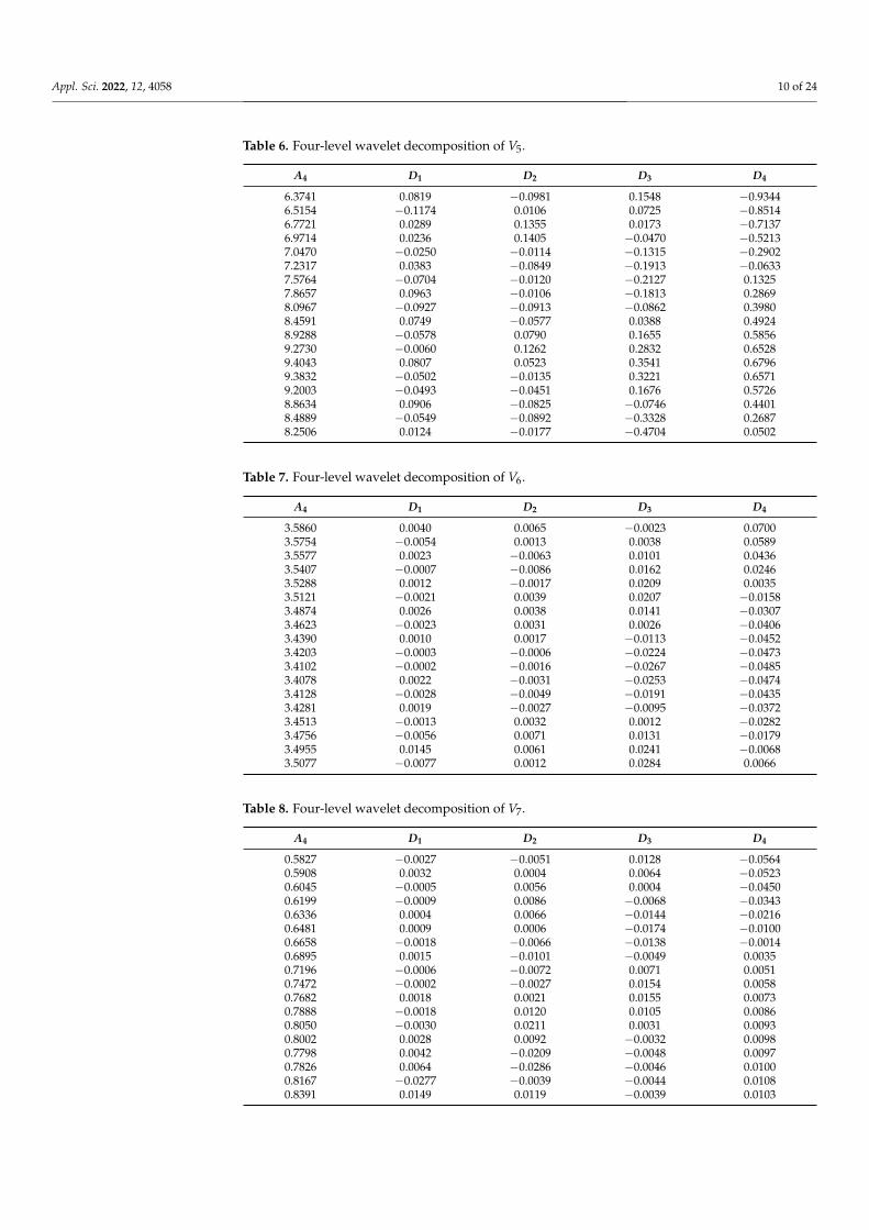
Next, we provide the wavelet multiscale analysis of each variable at the level 4, usingherewith the well-known Daubechies wavelet Db8 (See [34]). Tables 2–9 represent the fourcomponents due to the four-level wavelet decomposition. The first column in each tablerepresents the approximation component A4 relative to each variable, and the second, third,fourth, and fifth columns represent, respectively, the detail components D1, D2, D3, and D4already for each variable.

Table 2. Four-level wavelet decomposition of V1.

A4 D1 D2 D3 D4

13.6398 −0.0359 −0.1138 −0.0672 −0.350513.7696 0.0158 −0.0194 −0.1024 −0.298013.9706 0.0526 0.0865 −0.1073 −0.224514.1841 −0.0240 0.1539 −0.0883 −0.132114.3258 −0.0664 0.1181 −0.0540 −0.030914.3779 0.1050 −0.0025 −0.0151 0.056114.3789 −0.0877 −0.1416 0.0164 0.114714.4705 0.0285 −0.1568 0.0446 0.141114.6995 0.0391 −0.0022 0.0693 0.136814.8639 −0.0332 0.1117 0.0815 0.119514.8761 −0.0310 0.0862 0.0788 0.102814.8139 0.0441 0.0099 0.0591 0.080314.7116 0.0015 −0.0846 0.0244 0.053514.6949 0.0037 −0.0927 −0.0091 0.029214.8253 −0.0611 0.0372 −0.0310 0.008514.9016 0.0330 0.0993 −0.0437 −0.001114.8549 0.0638 0.0241 −0.0467 0.000914.8311 −0.0457 −0.0238 −0.0424 −0.0005

Appl. Sci. 2022, 12, 4058 9 of 24

Table 3. Four-level wavelet decomposition of V2.

A4 D1 D2 D3 D4

11.0367 0.2053 2.0380 2.3487 0.36668.6928 −0.7348 −0.1612 2.3803 0.38794.7299 0.8441 −2.7730 1.2976 0.38782.4961 0.2919 −2.8414 −0.5104 0.36553.4032 −1.5562 0.3882 −2.4143 0.34003.3979 2.8521 1.7395 −3.3599 0.36241.8750 −3.9350 −0.1305 −2.6500 0.45903.3736 1.6664 −0.0957 −0.8784 0.62987.3882 2.6088 2.0807 1.2229 0.85887.8662 −2.4552 1.4130 2.6468 1.08654.0935 −1.3945 −1.9316 2.5602 1.26151.9360 1.7160 −2.7348 1.5977 1.37962.7195 1.3865 −0.2637 0.3630 1.41432.7536 −1.0836 1.3615 −0.6843 1.32321.6384 −2.3794 1.1667 −0.9664 1.08900.3848 2.0492 0.6175 −0.9308 0.7000−1.3631 1.6941 −0.3359 −0.9063 0.1747−2.5174 −1.5886 −0.8588 −0.7252 −0.4095

Table 4. Four-level wavelet decomposition of V3.

A4 D1 D2 D3 D4

37.0951 −2.2791 −4.7882 −3.3139 −0.922540.8820 1.2570 −1.2043 −3.9412 0.359645.8691 2.7839 3.0641 −3.9847 1.704250.3946 −1.8896 6.2395 −3.2464 3.022751.3069 −2.3799 5.3467 −1.7768 4.173647.6891 5.0629 0.1665 −0.0998 4.954941.8344 −5.2364 −6.5255 1.4147 5.229841.5055 2.0575 −6.8480 2.6718 4.963148.5453 2.0447 1.2520 3.4202 4.186451.2447 −2.3167 6.1430 3.4182 3.063245.0606 −0.4526 3.1558 2.6198 1.758836.3746 2.5494 −1.4576 1.0723 0.326028.0662 −2.5642 −5.3802 −0.8362 −1.086925.5446 1.6904 −4.4002 −2.1723 −2.238231.4484 −1.0774 3.3774 −2.3684 −2.975934.3101 −1.0831 6.6704 −1.6996 −3.219029.7973 3.7997 1.5103 −0.5234 −2.982827.1184 −1.8634 −1.9759 0.4517 −2.4919

Table 5. Four-level wavelet decomposition of V4.

A4 D1 D2 D3 D4

5.5492 0.0108 −0.3690 0.1172 0.34015.8074 0.0126 −0.0491 0.0873 0.26606.1869 −0.1369 0.4061 0.0523 0.17186.1765 0.0735 0.4915 0.0045 0.05955.5848 0.1452 0.0031 −0.0473 −0.06555.2344 −0.1544 −0.2899 −0.0586 −0.19215.4054 −0.0254 −0.1292 −0.0141 −0.31175.5504 −0.0004 −0.0428 0.0625 −0.41915.5898 0.1802 −0.0772 0.1350 −0.51005.6454 −0.1254 −0.0351 0.1282 −0.58455.6183 −0.0483 0.0229 0.0020 −0.64015.6269 0.0931 0.1455 −0.1822 −0.66595.7274 −0.1374 0.3050 −0.3481 −0.65195.6632 −0.0132 0.1288 −0.3870 −0.58905.5373 0.3527 −0.3559 −0.2270 −0.47065.9918 0.0482 −0.4165 0.0472 −0.30217.0382 −0.9082 0.0746 0.3288 −0.09187.6892 0.5308 0.2793 0.4812 0.1488

Appl. Sci. 2022, 12, 4058 10 of 24

Table 6. Four-level wavelet decomposition of V5.

A4 D1 D2 D3 D4

6.3741 0.0819 −0.0981 0.1548 −0.93446.5154 −0.1174 0.0106 0.0725 −0.85146.7721 0.0289 0.1355 0.0173 −0.71376.9714 0.0236 0.1405 −0.0470 −0.52137.0470 −0.0250 −0.0114 −0.1315 −0.29027.2317 0.0383 −0.0849 −0.1913 −0.06337.5764 −0.0704 −0.0120 −0.2127 0.13257.8657 0.0963 −0.0106 −0.1813 0.28698.0967 −0.0927 −0.0913 −0.0862 0.39808.4591 0.0749 −0.0577 0.0388 0.49248.9288 −0.0578 0.0790 0.1655 0.58569.2730 −0.0060 0.1262 0.2832 0.65289.4043 0.0807 0.0523 0.3541 0.67969.3832 −0.0502 −0.0135 0.3221 0.65719.2003 −0.0493 −0.0451 0.1676 0.57268.8634 0.0906 −0.0825 −0.0746 0.44018.4889 −0.0549 −0.0892 −0.3328 0.26878.2506 0.0124 −0.0177 −0.4704 0.0502

Table 7. Four-level wavelet decomposition of V6.

A4 D1 D2 D3 D4

3.5860 0.0040 0.0065 −0.0023 0.07003.5754 −0.0054 0.0013 0.0038 0.05893.5577 0.0023 −0.0063 0.0101 0.04363.5407 −0.0007 −0.0086 0.0162 0.02463.5288 0.0012 −0.0017 0.0209 0.00353.5121 −0.0021 0.0039 0.0207 −0.01583.4874 0.0026 0.0038 0.0141 −0.03073.4623 −0.0023 0.0031 0.0026 −0.04063.4390 0.0010 0.0017 −0.0113 −0.04523.4203 −0.0003 −0.0006 −0.0224 −0.04733.4102 −0.0002 −0.0016 −0.0267 −0.04853.4078 0.0022 −0.0031 −0.0253 −0.04743.4128 −0.0028 −0.0049 −0.0191 −0.04353.4281 0.0019 −0.0027 −0.0095 −0.03723.4513 −0.0013 0.0032 0.0012 −0.02823.4756 −0.0056 0.0071 0.0131 −0.01793.4955 0.0145 0.0061 0.0241 −0.00683.5077 −0.0077 0.0012 0.0284 0.0066

Table 8. Four-level wavelet decomposition of V7.

A4 D1 D2 D3 D4

0.5827 −0.0027 −0.0051 0.0128 −0.05640.5908 0.0032 0.0004 0.0064 −0.05230.6045 −0.0005 0.0056 0.0004 −0.04500.6199 −0.0009 0.0086 −0.0068 −0.03430.6336 0.0004 0.0066 −0.0144 −0.02160.6481 0.0009 0.0006 −0.0174 −0.01000.6658 −0.0018 −0.0066 −0.0138 −0.00140.6895 0.0015 −0.0101 −0.0049 0.00350.7196 −0.0006 −0.0072 0.0071 0.00510.7472 −0.0002 −0.0027 0.0154 0.00580.7682 0.0018 0.0021 0.0155 0.00730.7888 −0.0018 0.0120 0.0105 0.00860.8050 −0.0030 0.0211 0.0031 0.00930.8002 0.0028 0.0092 −0.0032 0.00980.7798 0.0042 −0.0209 −0.0048 0.00970.7826 0.0064 −0.0286 −0.0046 0.01000.8167 −0.0277 −0.0039 −0.0044 0.01080.8391 0.0149 0.0119 −0.0039 0.0103

Appl. Sci. 2022, 12, 4058 11 of 24

Table 9. Four-level wavelet decomposition of V8.

A4 D1 D2 D3 D4

73.0235 −0.0135 −0.0375 0.0975 −0.361073.0854 0.0146 0.0010 0.0649 −0.352073.1909 −0.0009 0.0442 0.0323 −0.321773.2898 −0.0098 0.0527 −0.0116 −0.269273.3579 0.0121 0.0091 −0.0639 −0.201673.4667 −0.0067 −0.0234 −0.0914 −0.139573.6397 0.0003 −0.0189 −0.0813 −0.095173.8266 0.0034 −0.0166 −0.0399 −0.071074.0156 −0.0056 −0.0171 0.0210 −0.065674.2021 −0.0021 −0.0032 0.0628 −0.061674.3624 0.0176 0.0149 0.0602 −0.047274.4935 −0.0135 0.0268 0.0330 −0.030074.5991 −0.0091 0.0261 −0.0029 −0.011874.6850 0.0050 −0.0000 −0.0278 0.009274.7759 0.0241 −0.0399 −0.0223 0.030674.9135 −0.0135 −0.0373 −0.0056 0.057875.0896 −0.0296 0.0159 0.0072 0.090875.2003 0.0197 0.0346 0.0133 0.1159

As we know, it is generally not easy to see accurately the variations (fluctuations,increase, decrease) of these variables from the tables solely. So, for further understandingthe behavior of these variables according to the time scale, we reproduced the variables Viof Table 1 to illustrate more their variability of their behaviors. This will yield in turn andamong other interpretations a good and easy reading and description of these variablesaccording to the time scale. The following graphs illustrate the variables with their trendsand dynamics or fluctuations represented by the four-level wavelet decomposition (seeFigures 1–8). The strong fitting between each variable and its approximation is clearlynoticed, which is always and already confirmed in wavelet theory.

Figure 1. The wavelet decomposition of the variable V1 at the level 4.

Appl. Sci. 2022, 12, 4058 12 of 24

Figure 2. The wavelet decomposition of the variable V2 at the level 4.

Figure 3. The wavelet decomposition of the variable V3 at the level 4.

Appl. Sci. 2022, 12, 4058 13 of 24

Figure 4. The wavelet decomposition of the variable V4 at the level 4.

Figure 5. The wavelet decomposition of the variable V5 at the level 4.

Appl. Sci. 2022, 12, 4058 14 of 24

Figure 6. The wavelet decomposition of the variable V6 at the level 4.

Figure 7. The wavelet decomposition of the variable V7 at the level 4.

Appl. Sci. 2022, 12, 4058 15 of 24

Figure 8. The wavelet decomposition of the variable V8 at the level 4.

Next, as the components of our sample are completed and the sample has now nomissing values, we provide the resulting quality of life index HDI issued from the model (5).The values are provided in Table 10 below.

Table 10. The HDI index, real and time-scale model (5).

HDI0 HDI1 HDI2 HDI3 HDI4

0.7841 −0.0021 −0.0033 0.0046 −0.02840.7859 0.0021 0.0001 0.0019 −0.02600.7886 0.0004 0.0033 −0.0003 −0.02200.7920 −0.0007 0.0048 −0.0028 −0.01640.7962 −0.0010 0.0030 −0.0055 −0.00960.8008 0.0019 −0.0007 −0.0067 −0.00330.8057 −0.0016 −0.0039 −0.0059 0.00170.8108 0.0007 −0.0044 −0.0032 0.00500.8161 0.0002 −0.0012 0.0011 0.00680.8216 −0.0007 0.0013 0.0047 0.00800.8273 0.0004 0.0014 0.0063 0.00950.8329 −0.0004 0.0024 0.0065 0.01060.8383 0.0007 0.0037 0.0054 0.01100.8432 0.0004 0.0014 0.0033 0.01070.8477 −0.0024 −0.0036 0.0008 0.00960.8515 0.0020 −0.0052 −0.0023 0.00810.8547 0.0005 −0.0018 −0.0056 0.00620.8572 −0.0008 0.0013 −0.0071 0.0034

Figure 9 illustrates graphically the behavior of the quality of life index HDI andprovides thus a graphical comparison between the real values and the one due to ourwavelet multiscale model (5).

Appl. Sci. 2022, 12, 4058 16 of 24

Figure 9. The plots of the HDI index, real and time scale model (5).

6. Discussion of Results

Before going on commenting and discussing our results in the framework of quality oflife sense, we quickly recall some facts about the accuracy and convergence of our waveletdecomposition. This may be in fact a theoretical task which is already guaranteed in wavelettheory. We know that in wavelet theory, the wavelet approximation of the statistical seriesat a level J converges in the L2-sense (variance or standard deviation measures in statistics).Mathematically speaking, we know that the projection on the multi-resolution space VJguarantees an approximation of the order 2−sJ , and thus, as we increase the order J, we keepa best convergence and accuracy. s = NLogN is the regularity of the wavelet used, whereN is the length of the wavelet filter. In our case, Db8 is regular of order s = 8Log8 = 16.63.So, the order of convergence is approximately 2−32Log8, which is an accurate order.

Let us now comment on, interpret, and discuss our empirical results. Figure 1 illus-trates the behavior of the variable V1, which represents the Gross Domestic Product. Noticethat such a variable represents a global shape showing an increase in time. However, itsglobal shape does not reflect the real and hidden behavior of the variable according to thetime scale. Indeed, at low scales, j = 1, the component D1 shows quietly the same globalbehavior, an increasing variation according to time. However, by increasing the level or thescale, the real hidden behavior starts to appear, explaining some pseudo-periodicity and/ora fluctuation in the variation of the factor V1. By means of quality of life vocabulary, thismeans that the situation is not stable, and thus, the future quality of life situation shouldbe carefully linked to the Gross Domestic Product. However, this is unstable accordingto the time scale. Related to the case study, especially the period chosen, this is a naturalconsequence of many critical phenomena that happened in this period. The first is thestarting steps in implementing the 2030 vision plans. As usual, with the absence of a realfuture view, precise forecasting, and prevision of this plan, the statistics as well as thereal behavior of investors and citizens is always careful. The COVID-19 pandemic hasbeen also dispersed in all the word, leading to a perturbation and sometimes a permanentstop of many important activities such as oil exportation, foreign investments, etc. Thesefacts affect the local or the national market, especially local or domestic production: for

Appl. Sci. 2022, 12, 4058 17 of 24

example, by increasing prices of consummations, taxes, etc, which negatively affect theview of people regarding their lives, especially their economic situation.

The variable V2 representing the Gross National Income is tending more toward adecreasing shape, with more stability at medium horizons. As the time scale increases, thisincome shows more instability with always a decreasing magnitude. This may be due asevoked previously to many causes, especially COVID-19, as well as the low movementof exportation. Recall also that the embargo against Qatar country where the exportationof a big amount of especially food industry products has been stopped for a long time, asestimated by the level j = 3. Another cause is the restoring legitimacy of the war in Yemen,which has largely affected the GCC continent in general. These phenomena have led to alarge portion of money being directed to and reserved for the army activities and needsrather than being allocated to investments that bring more interest to the treasury.

The variable V3 relative to Gross Savings is somehow increasing in low horizons, witha small perturbation in medium levels, and more instabilities at higher horizons. Thisbehavior may be explained by the fact that the present or precisely the index is high atthe beginning of the period, and then it starts to be unstable, decreasing as the time scaleincreases. A main cause is firstly the increase in prices mainly of consumed products, forwhich COVID-19 stopped many, even small, activities. There was an increase of taxes aswell as fuel prices and cars. An important movement of immigration of citizens and thusan outside flow of money investments has taken place.

The employment rate denoted here by V4 according to Figure 4 is somehow remainingstable and quietly constant with little variation from its average, especially at short horizons.At the end of the period, there is an extreme increase or what we call jump, which may beexplained by the movement of nationalization of jobs in the kingdom as part of the politicsof the government already in the application and/or the execution of the 2030 vision planto reduce the national unemployment rate. We know that Saudi Arabia, as well as thewhole continent of GCC countries, rely on a large percentage on foreign incoming laborfrom abroad. GCC countries have planned some 2030 to 2035 vision plans, which targetamong many goals reducing the non-national labor. However, in the last period, manycrises have appeared such as the COVID-19 pandemic as well as the Yemen war, whichseverely affected the economy. Many industrial as well as small firms have been closed dueto the crisis. This explains well the increase of the unemployment rate suddenly. However,we stress that this instability is not large enough to affect strongly the variation of theunemployment rate. It is worthy recalling that Saudi nationals are not widely attracting theprivate sector, as they are on one side seeking high salaries, and on the other side, they havemore employment protections than expatriate workers, The government has made somepolicy to encourage the private sector for Saudi nationals recruitment such as the Nitaqat,which allocates some funds to private firms that recruit Saudi nationals. This policy haseffectively increased the employment rate in some short time horizons. However, withthe not strong qualifications of this national labor, the private sector often replaces theseworkers with expatriates, which caused in turn many problems.

The variable V5 designates the Energy Consumption per Capita. Concerning thisindex, Saudi Arabia is one of the most important countries and forces that may provide theentire population with self-produced energy. Moreover, it may produce more energy, whichis then exported. This makes the index of Energy Consumption globally increasing in shorthorizons, as it is shown in Figure 5. This may be naturally explained by the availability ofenergy to be delivered to the population time-wise. However, at long horizons, we noticesome perturbation shown clearly in the detail component D4 relative to this factor. Thisexplains the influence of the global crisis due to COVID-19 and the Yemen war, which hasled to a lack of technology importation as a main cause (see also [54]). We may also hererelate this perturbation to the act of nationalization of jobs when including non-qualifiedjobs. One of the main plans in the 2030 vision is the NEOM city that the kingdom startedto implement in the northwest region. This project has a great influence as a great partof energy as well as a huge amount of money is now allocated to such a project. In other

Appl. Sci. 2022, 12, 4058 18 of 24

words, a type of austerity policy is carried out in order to save both energy and money forthe NEOM project.

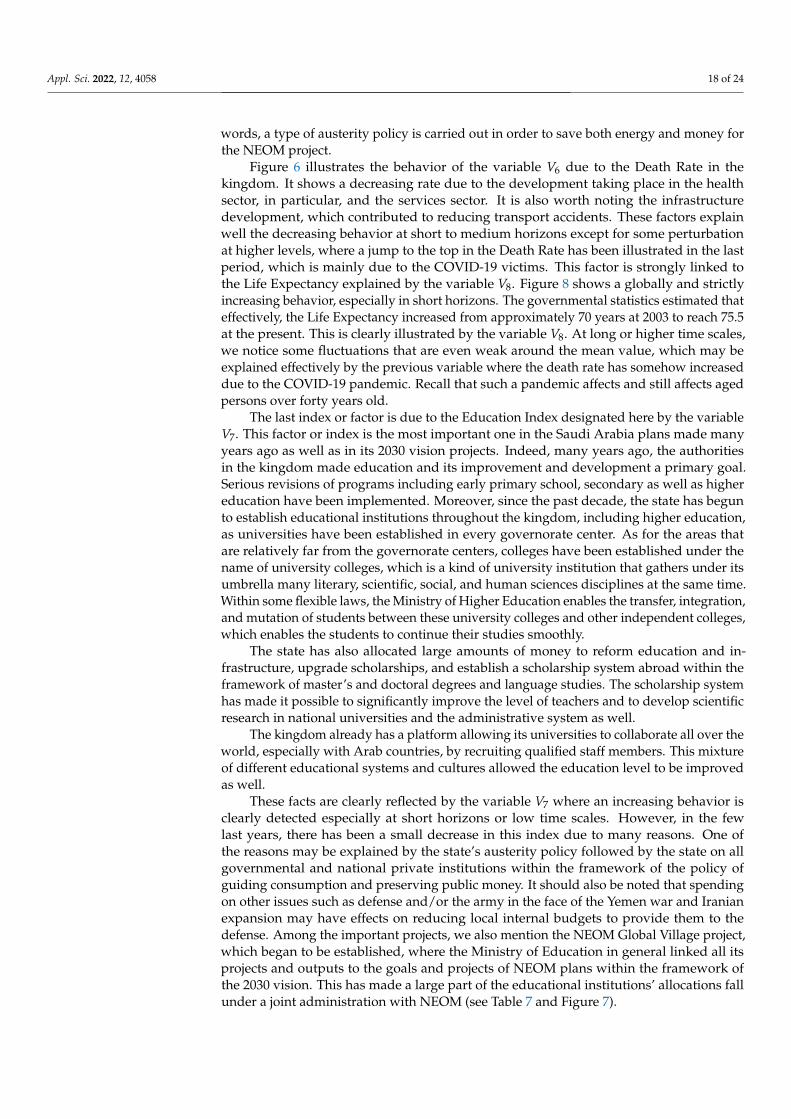
Figure 6 illustrates the behavior of the variable V6 due to the Death Rate in thekingdom. It shows a decreasing rate due to the development taking place in the healthsector, in particular, and the services sector. It is also worth noting the infrastructuredevelopment, which contributed to reducing transport accidents. These factors explainwell the decreasing behavior at short to medium horizons except for some perturbationat higher levels, where a jump to the top in the Death Rate has been illustrated in the lastperiod, which is mainly due to the COVID-19 victims. This factor is strongly linked tothe Life Expectancy explained by the variable V8. Figure 8 shows a globally and strictlyincreasing behavior, especially in short horizons. The governmental statistics estimated thateffectively, the Life Expectancy increased from approximately 70 years at 2003 to reach 75.5at the present. This is clearly illustrated by the variable V8. At long or higher time scales,we notice some fluctuations that are even weak around the mean value, which may beexplained effectively by the previous variable where the death rate has somehow increaseddue to the COVID-19 pandemic. Recall that such a pandemic affects and still affects agedpersons over forty years old.

The last index or factor is due to the Education Index designated here by the variableV7. This factor or index is the most important one in the Saudi Arabia plans made manyyears ago as well as in its 2030 vision projects. Indeed, many years ago, the authoritiesin the kingdom made education and its improvement and development a primary goal.Serious revisions of programs including early primary school, secondary as well as highereducation have been implemented. Moreover, since the past decade, the state has begunto establish educational institutions throughout the kingdom, including higher education,as universities have been established in every governorate center. As for the areas thatare relatively far from the governorate centers, colleges have been established under thename of university colleges, which is a kind of university institution that gathers under itsumbrella many literary, scientific, social, and human sciences disciplines at the same time.Within some flexible laws, the Ministry of Higher Education enables the transfer, integration,and mutation of students between these university colleges and other independent colleges,which enables the students to continue their studies smoothly.

The state has also allocated large amounts of money to reform education and in-frastructure, upgrade scholarships, and establish a scholarship system abroad within theframework of master’s and doctoral degrees and language studies. The scholarship systemhas made it possible to significantly improve the level of teachers and to develop scientificresearch in national universities and the administrative system as well.

The kingdom already has a platform allowing its universities to collaborate all over theworld, especially with Arab countries, by recruiting qualified staff members. This mixtureof different educational systems and cultures allowed the education level to be improvedas well.

These facts are clearly reflected by the variable V7 where an increasing behavior isclearly detected especially at short horizons or low time scales. However, in the fewlast years, there has been a small decrease in this index due to many reasons. One ofthe reasons may be explained by the state’s austerity policy followed by the state on allgovernmental and national private institutions within the framework of the policy ofguiding consumption and preserving public money. It should also be noted that spendingon other issues such as defense and/or the army in the face of the Yemen war and Iranianexpansion may have effects on reducing local internal budgets to provide them to thedefense. Among the important projects, we also mention the NEOM Global Village project,which began to be established, where the Ministry of Education in general linked all itsprojects and outputs to the goals and projects of NEOM plans within the framework ofthe 2030 vision. This has made a large part of the educational institutions’ allocations fallunder a joint administration with NEOM (see Table 7 and Figure 7).

Appl. Sci. 2022, 12, 4058 19 of 24

Now, as the components of our sample are illustrated, described, analyzed, andinterpreted, we provide the resulting quality of life index HDI issued from the model (5).The values are provided in Table 10 below.

Notice from Table 10 and Figure 9 that the wavelet multiscale model succeeded toreflect or to localize the real behavior of the HDI relative to time scales. Contrarily toexisting methods that yield a global value on each a priory fixed period independent fromeach other, and to the scale, we here notice that the HDI may possess different time-scalebehaviors. Related to the case study, the HDI is increasing at short to medium horizons,reflecting good well-being and/or satisfaction versus the quality of life in the kingdom,especially at the beginning of the period of study.

Overall, the present study concludes clearly and strongly that time-scale decomposi-tion is very important for analyzing quality of life index as well as its factors. In particular,we conclude easily that the case study of Saudi Arabia during the period 2003–2020 is anappropriate period to model the quality of life index at the time scale, which is clearlydominated by a trend. At higher scales (i.e., low frequencies), the wavelet details permitlocalizing the instabilities in the index behavior and thus allow the researchers to analyzethe eventual causes. In low horizons, the fit is generally well.

Existing models dealing with the quality of life are in the majority independentlybased on the health situation or economic one. So, only the influence of the health situationof individuals or the influence of the economical variables are estimated in these models.However, there may be many dimensions and factors that influence the population life andtheir satisfaction such as education, security, employment, etc. The present model, even ithas not considered all the facts related to quality of life, tried to include many of them toestimate a more adequate index.

7. Conclusions

The present paper concerns the estimation of a quality of life index by using wavelettheory as a mathematical tool to discover the influence of the time scale on such an index.The wavelet multiscale then provided allowed the estimation of the quality of life index inSaudi Arabia.

In the present work, we developed a quantitative mathematical model for estimatingthe quality of life index. The first step in building the model is a wavelet by adjusting thedatabase. Such a base is characterized by its short size, which represents a major drawbackin the prediction of statistical series. We showed that on the contrary, wavelets are able toremedy such a problem. The model is then applied to Saudi Arabia as a case study in theframework of its 2030 vision plan, and it is based on data gathered from social media.

The results show firstly the effectiveness of wavelets in the development of multiscale-in-time models, and secondly, the effect of the time scale in the description of the behaviorof the index of quality of life and its variation over time. The present model permits thepossibility to overcome the subjectivity and intangibility of the major existing models,which are majorly non-quantitative, and allows thus a quantification of the quality oflife index.

The present work confirms the idea stating that generally, to estimate quality oflife or population satisfaction and well-being, it is necessary to define the areas wherethe individuals can realize their possibilities at different levels, such as the availabilityof services, health care, education, security and safety (economic and physical), dignity,communication, participation in decision making, etc.

The present model may be improved to include more dimensions such as materialliving standards, political voice and governance, social connections and relationships,environment, etc. We join here the models discussed theoretically in [52,53]. We think thata hybrid idea may lead to better estimates and understanding of the quality of life index.A future eventual extension of the present study may be also the consideration of factoranalysis as a classical tool, especially in social sciences.

Appl. Sci. 2022, 12, 4058 20 of 24

The present model may be also improved in the step of wavelet adjustment of thedata, where missing values have been reconstructed. An extension of the datasets may beapplied by considering long series (with large size) to be used for forecasting the missingvalues and next extract the adequate sub-series relative to the period of study. This permitslong time series in the forecasting. Recall that effectively, the use of long time series yieldsthe best accuracy and convergence of the wavelet approximation.

Author Contributions: Conceptualization, M.S.B. and A.B.M.; Methodology, M.S.B. and A.B.M.;Software, M.S.B. and A.B.M.; Validation, M.S.B. and A.B.M.; Formal analysis, M.S.B. and A.B.M.;Investigation, M.S.B. and A.B.M.; Resources, M.S.B. and A.B.M.; Data curation, M.S.B. and A.B.M.;Writing—original draft preparation, M.S.B. and A.B.M.; Writing—review and editing, M.S.B. andA.B.M.; Visualization, M.S.B. and A.B.M.; Supervision, M.S.B. and A.B.M.; Project administration,M.S.B. and A.B.M.; Funding acquisition, M.S.B. and A.B.M. All authors have read and agreed to thepublished version of the manuscript.

Funding: This research received no external funding.

Institutional Review Board Statement: Not applicable.

Informed Consent Statement: Not applicable.

Data Availability Statement: Not Applicable

Conflicts of Interest: The authors declare no conflict of interest.

Appendix A. Wavelet Processing Toolkit

Wavelets have been introduced few decades ago in mathematical theory, althoughtheir discovery was related to applications in petroleum extraction [12–16,34].

A wavelet is simply a short wave function oscillating such as the Fourier modes, butwith high frequency and small support, which we call in wavelet theory localization intime-frequency and/or time-space.

To analyze a statistical (time, financial, etc.) series, we have to compute the so-called wavelet transform, a two-parameter quantity evaluated by the correlation type (aconvolution) of the analyzed series with translated-dilated copies of one fixed waveletknown as the mother wavelet, which is a special function that should satisfy at least anadmissibility assumption as

Aψ =∫R

|ψ̂(ξ)|2|ξ| dξ < ∞. (A1)

The wavelet analysis appeared originally in the theoretical form as a refinement andalso terminology to Fourier and harmonic analysis is general. Therefore, it associates tothe analyzed function a type of transform known as the wavelet transform or exactly thecontinuous wavelet transform obtained by a convolution product of the analyzed functionwith special copies of a source function known as the mother wavelet. More precisely,denote for s > 0 and u ∈ R fixed

ψs,u(x) =1√

sψ(

x− us

). (A2)

For a function F ∈ L2(R), its continuous wavelet transform at the scale s and theposition u is defined by

WT s,u(F) =∫ ∞

−∞F(t)ψs,u(t)dt. (A3)

The parameters s and u have many nominations according to the context of use of thewavelet transform. s is known as a frequency, scale, or a dilation or compression parameter.u is known also as the translation parameter. When covering all the real values of s andu, we obtain the so-called time-frequency or time-space domain. This transform is called

Appl. Sci. 2022, 12, 4058 21 of 24

continuous because of the nature of the parameters s and u that may operate on all thespace (0, ∞)× R. It holds in wavelet theory that the function F may be reproduced bymeans of its continuous wavelet transform in an L2-sense and analogously as in Fourieranalysis via the L2-equality

F(t) =1Aψ

∫ ∫RWT u,s(F)ψ

(x− u

s

)dsdu

s2 . (A4)

We conclude that the wavelet transform operates according two parameters: theparameter s permitting to compress or to dilate the graph of ψ, which allows in turn toreach the high/low magnitude fluctuations in the signal, and the parameter u, whichpermits translating the graph of ψ to localize or to approach the local fluctuations.

The discrete wavelet transform is a variant of the continuous one evaluated on adiscrete grid for the parameters s and u. The most known one is the dyadic, while there isno essential difference between the discrete grids. In the dyadic case, we restrict on the set{(s, u) = (2−j, k2−j) ; j, k ∈ Z}. In this case, the translated–dilated copies are defined by

ψj,k(t) = 2j/2ψ(2jt− k). (A5)

The continuous wavelet transformWT s,u will be called the discrete wavelet transform,which is denoted usually by dj,k. The recosntruction formula (A6) will be evaluated via adiscrete representation as

F(t) = ∑j,k

dj,k(F)ψj,k(t), (A6)

known as the wavelet series of the function F.In the discrete case such as statistical series and discrete signals, the wavelet transform

of a series X(t) (known also as the discrete wavelet transform (DWT)) is obtained bycorrelation-type (discrete convolution)

dj,k(X) = ∑n

X(n)ψj,k(n), (A7)

known also as the wavelet coefficient or detail coefficient at the level or the scale j and theposition k. In wavelet theory, it is proved that any series X(t) may be decomposed in aseries form as

X(t) = ∑j,k

dj,k(X)ψj,k(t), (A8)

known as the wavelet series or the wavelet decomposition of X(t), and it guarantees acomplete reconstruction formula of the original series X(t) [12–19,33,34].

The greatest advantage of this decomposition is the fact that it allows splitting thedata into different horizons known as levels. Each level is associated to a component ofthe series, and it makes itself a refinement of the preceding one, which we call in wavelettheory the concept of multi-resolution. Denote for j ∈ Z, Wj = spann(ψj,k ; k ∈ Z) (known

as the detail space at the level j), and Vj =⊥⊕

l≤j

Wl (known as the approximation space at

the level j). We get an orthogonal decomposition Vj = Vj−1

⊥⊕Wj−1. This permits splitting

the wavelet decomposition above as

X(t) = ∑j≤Jmin,k

dj,k(X)ψj,k(t) + ∑j>Jmin,k

dj,k(X)ψj,k(t), (A9)

relative to a fixed integer Jmin ∈ Z. For j ∈ Z, the component

Appl. Sci. 2022, 12, 4058 22 of 24

Aj(X(t)) = ∑l≤j,k

dl,k(X)ψl,k(t) (A10)

belongs to Vj, and it is called the approximation of X(t) at the level j. It describes the globalbehavior, the trend, or the shape of X(t). The component

Dj(X(t)) = ∑k

dj,k(X)ψj,k(t) (A11)

belongs to the space Wj, and it is called the detail component of X(t) at the level j. It reflectsthe higher frequency oscillations or the fine-scale deviations of the series near its trend. Asa consequence, the wavelet decomposition of X(t) in (A9) is a superposition as

X(t) = AJmin(X(t)) + DJmin+1(X(t)) + DJmin+2(X(t)) + . . . (A12)

A second main advantage of wavelet theory is the reduction in computing the coeffi-cients needed in the decomposition. Indeed, there exists a function ϕ (known as the scalingfunction or the father wavelet) characterized by the so-called two-scale relation

ϕ = ∑k∈Z

hk ϕ1,k, (A13)

and which is related to the function ψ by

ψ = ∑k∈Z

gk ϕ1,k, (A14)

where

hk =∫ +∞

−∞ϕ(t)ϕ1,k(t)dt, and gk = (−1)kh1−k. (A15)

It holds that Vj = spann(ϕj,k ; k ∈ Z), where the ϕj,k values are defined similarly tothe ψj,k in (A5). The component Aj(X(t)) is therefore written as

Aj(X(t)) = ∑k

aj,k(X)ϕj,k(t), (A16)

where the coefficients aj,k(X) (known as the approximation or scaling coefficients of X(t))are evaluated as the dj,k(X) by replacing the function ψ by ϕ. The relation (A13) permitscomputing the level decomposition from each other as

aj,k(X) = ∑l∈Z

hlaj+1,l+2k(X), (A17)

dj,k(X) = ∑l∈Z

glaj+1,l+2k(X), (A18)

andaj+1,k(X) = ∑

lhl−2kaj,l(X) + ∑

lgl−2kdj,l(X). (A19)

The sequence H = (hk)k is called the discrete wavelet low-pass filter, and the sequenceG = (gk)k is the discrete wavelet high-pass filter.

The truncation of the last decomposition in (A12) in a practical finite level J > Jmin ∈ Zgives the so-called J-level finite wavelet decomposition of X(t) as

SJ = AJ0(S) + ∑J0<j≤J

Dj(S). (A20)

Appl. Sci. 2022, 12, 4058 23 of 24

The lower index Jmin is in fact more flexible, and it is usually chosen to be 0. Thechoice of J is always critical, and it is related to the eventual error estimates requested.See [12–16,34] for more details.

References1. Caescu, S.C.; Constantinescu, M.; Ploesteanu, M.G. Strategic Marketing and Quality of Life; Annals of Faculty of Economics; Faculty

of Economics, University of Oradea: Oradea, Romania, 2012; Volume 1, pp. 801–806.2. Cella, D.F.; Cherin, E.A. Quality of life during and after cancer treatment. Compr Ther. 1988, 14, 69–75. [PubMed]3. Colby, B.N. Well-Being: A Theoretical Program. Am. Anthropol. 1987, 89, 879–895. [CrossRef]4. Bucur, B. How can we apply the models of the quality of life and the quality of life management in an economy based on

knowledge? Econ. Res. Ekon. Istraz. 2017, 30, 629–646. [CrossRef]5. Bucur, A. Modeling as a multiple-criteria decision-making problem and simulation, for the hierarchization of programs of study.

In Proceedings of the Advances in Automatic Control Modelling and Simulation, Brasov, Romania, 1–3 June 2013; pp. 338–343.6. Bucur, A. An indicator of an individual’s professional quality. In Proceedings of the 8th International Conference on Applied

Mathematics, Simulation, Modelling, Florence, Italy, 22–24 November 2014; pp. 342–345.7. Bucur, A.; Oprean, C. Operational Research and Applications in Quality Management; LAP Lambert Academic Publishing: Saar-

brücken, Germany, 2014.8. Costanza, R.; Fisher, B.; Ali, S.; Beer, C.; Bond, L.; Boumans, R.; Snapp, R. An integrative approach to quality of life measurement,

research, and policy. Surv. Perspect. Integr. Environ. Soc. 2008, 1, 16–21. [CrossRef]9. Fayers, P.M.; Machin, D. Quality of Life the Assessment, Analysis and Interpretation of Patient-Reported Outcomes, 2nd ed.; John Wiley

& Sons, Ltd.: West Sussex, UK, 2007.10. Alves, H.; Vázquez, J.L. Quality-of-Life Marketing: An Introduction to the Topic. In Best Practices in Marketing and Their

Impact on Quality of Life; Applying Quality of Life Research: (Best Practices); Alves, H., Vázquez, J., Eds.; Springer: Dordrecht,The Netherlands, 2013.

11. Quality of Life Program Delivery Plan. Available online: https://www.vision2030.gov.sa/v2030/vrps/qol (accessed on 1 January 2022).12. Arfaoui, S.; Rezgui, I.; Ben Mabrouk, A. Wavelet Analysis on the Sphere; Spheroidal Wavelets; De Gryuter: Berlin, Germany, 2017.13. Arfaoui, S.; Ben Mabrouk, A.; Cattani, C. Wavelet Analysis Basic Concepts and Applications, 1st ed.; CRC Taylor-Francis, Chapmann

& Hall: Boca Raton, FL, USA, 2021.14. Gençay, R.; Selçuk, F.; Whitcher, B. An Introduction to Wavelets and Other Filtering Methods in Finance and Economics; Academic

Press: San Diego, CA, USA, 2002.15. Hubbard, B.B. The World According to Wavelets: The Story of a Mathematical Technique in the Making, 2nd ed.; Ak Peters Ltd.: Natick,

MA, USA, 1998.16. Mallat, S. A Wavelet Tour of Signal Processing, 3rd ed.; The Sparse Way, Academic Press: Orlando, FL, USA, 2008.17. Sarraj, M.; Ben Mabrouk, A. The Systematic Risk at the Crisis-A Multifractal Non-Uniform Wavelet Systematic Risk Estimation.

Fractal Fract. 2021, 5, 135. [CrossRef]18. Soltani, S. On the use of the wavelet decomposition for time series prediction. Neurocomputing 2002, 48, 267–277. [CrossRef]19. Soltani, S.; Modarres, R.; Eslamian, S.S. The use of time series modeling for the determination of rainfall climates of Iran. Int. J.

Climatol. 2007, 27, 819–829. [CrossRef]20. Faes, L.; Porta, A.; Javorka, M.; Nollo, G. Efficient Computation of Multiscale Entropy over Short Biomedical Time Series Based

on Linear State-Space Models. Complexity 2017, 2017, 1768264. [CrossRef]21. Messer, M.; Backhaus, H.; Fu, T.; Stroh, A.; Schneider, G. A multi-scale approach for testing and detecting peaks in time series.

Statistics 2020, 54, 1058–1080. [CrossRef]22. Wang, J.; Shang, P.; Zhao, X.; Xia, J. Multiscale entropy analysis of traffic time series. Int. J. Mod. Phys. C 2013, 24, 1350006.

[CrossRef]23. Wu, S.-D.; Wu, C.-W.; Lin, S.-G.; Wang, C.-C.; Lee, K.-Y. Time Series Analysis Using Composite Multiscale Entropy. Entropy 2013,

15, 1069–1084. [CrossRef]24. Adam, T.; Oelschlger, L. Hidden Markov models for multi-scale time series: An application to stock market data. In Proceedings

of the 35th International Workshop on Statistical Modelling (IWSM), Bilbao, Spain, 19–24 July 2020; 6p.25. Baranowski, R.; Fryzlewicz, P. Multiscale autoregression on adaptively detected timescales. In Proceedings of the 12th Interna-

tional Conference of the ERCIM WG on Computational and Methodological Statistics (CMStatistics 2019), London, UK, 14–16December 2019.

26. Chen, L.; Ozsu, M.T.A. Similarity-Based Retrieval of Time-Series Data Using Multi-Scale Histograms; Technical Report CS-2003-31 Sept2003; School of Computer Science, University of Waterloo: Waterloo, ON, Canada; 26p.

27. Gierałtowski, J.; Zebrowski, J.J.; Baranowski, R. Multiscale multifractal analysis of heart rate variability recordings with a largenumber of occurrences of arrhythmia. Phys. Rev. E 2012, 85, 021915. [CrossRef] [PubMed]

28. Cai, B.; Huang, G.; Xiang, Y.; Angelova, M. Multi-Scale Shapelets Discovery for Time-Series Classification. Int. J. Inf. Technol.Decis. Mak. 2020, 19, 721–739. [CrossRef]

29. Shi, Y.; Li, B.; Du, G.; Dai, W. Clustering framework based on multi-scale analysis of intraday financial time series. Physica A 2021,567, 125728. [CrossRef]

Appl. Sci. 2022, 12, 4058 24 of 24

30. Cho, M.; Kim, B.; Bae, H.-J.; Seo, J. Stroscope: Multi-Scale Visualization of Irregularly Measured Time-Series Data. IEEE Trans. Vis.Comput. Graph. 2014, 20, 808–821. [CrossRef] [PubMed]

31. Vespier, U.; Knobbe, A.; Nijssen, S.; Vanschoren, J. MDL-based Analysis of Time Series at Multiple Time-Scales. ECMLPKDD’12.In Proceedings of the 2012th European Conference on Machine Learning and Knowledge Discovery in Databases, Bristol, UK,24–28 September 2012; Volume II, pp. 371–386.

32. Gao, J.; Cao, Y.; Tung, W.-W.; Hu, H. Multiscale Analysis of Complex Time Series: Integration of Chaos and Random Fractal Theory, andBeyond; John Wiley: Hoboken, NJ, USA, 2007.

33. Ben Mabrouk, A.; Kahloul, I.; Hallara, S.-E. Wavelet-Based Prediction for Governance, Diversification and Value CreationVariables. Int. Res. J. Financ. Econ. 2010, 60, 15–28.

34. Daubechies, I. Ten Lectures on Wavelets; Society for Industrial and Applied Mathematics: Philadelphia, PA, USA, 1992.35. Arndt, J. Marketing and the quality of life. J. Econ. Psychol. 1981, 1, 283–301. [CrossRef]36. Constantinescu, M. The Relationship between the Quality of Life Concept and Social Marketing Development. Int. J. Econ. Pract.

Theor. 2012, 2, 75–80.37. Hajli, M.N. A study of the impact of social media on consumers. Int. J. Mark. Res. 2014, 56, 387–404. [CrossRef]38. McCall, S. Quality of life. Soc. Indic. Res. 1975, 2, 229–248. [CrossRef]39. Michalos, A.C. (Ed.) Encyclopedia of Quality of Life and Well-Being Research; Springer: Berlin, Germany, 2014.40. Schuessler, K.F.; Fisher, G.A. Quality of life research and sociology. Annu. Rev. Sociol. 1985, 11, 129–149. [CrossRef]41. Siddiqui, S.; Singh, T. Social Media its Impact with Positive and Negative Aspects. Int. J. Comput. Appl. Technol. Res. 2016, 5,

71–75. [CrossRef]42. Sirgy, M.J.; Samli, A.C.; Meadow, H.L. The Interface between Quality of Life and Marketing: A Theoretical Framework. J. Mark.

Public Policy 1982, 1, 69–84. [CrossRef]43. Terhune, K.W. Probing policy relevant questions on the quality of life. In The Quality of Life Concept; Environmental Protection

Agency: Washington, DC, USA, 1973.44. Testa, M.A.; Simonson, D.C. Assessment of quality of life outcomes. N. Engl. J. Med. 1996, 334, 835–840. [CrossRef] [PubMed]45. Veenhoven, R. The four quality of life. Ordering concepts and measures of the good life. In Understanding Human Well-Being;

McGillivray, M., Clark, M., Eds.; United Nations University Press: Tokyo, Japan; NewYork, NY, USA; Paris, France, 2006;pp. 74–100.

46. Wilczek, B. Media Use and Life Satisfaction: The Moderating Role of Social Events. Int. Rev. Econ. 2018, 65, 157–184. [CrossRef]47. Jones, N.; Borgman, R.; Ulusoy, E. Impact of social media on small Businesses. J. Small Bus. Enterp. Dev. 2015, 22, 611–632.

[CrossRef]48. Lee, D.-J.; Sirgy, M.J. Quality-of-Life (QOL) Marketing: Proposed Antecedents and Consequences. J. Macromark. 2004, 24, 44–58.

[CrossRef]49. Sirgy, M.J.; Samli, A.C. New Dimensions in Marketing/Quality of Life Research; Quorum Books: Westport, CT, USA, 1995.50. Boscaiu, V.; Voda, V.G. Aplicatii ale seriilor de timp vectoriale in controlul calitatii, Applications of the vector time series in quality

control. Rev. Calit. Manag. 2008, 7, 42–45.51. Oprean, C.; Bucur, A. Modeling and simulation of the quality’s entropy. Qual. Quant. 2013, 47, 3403–3409. [CrossRef]52. Puskorius, S. Theoretical Model of Estimating the Quality of Life Index. Intelekt. Econ. 2014, 8, 55–64. [CrossRef]53. Puskorius, S. The Methodology of Calculation the Quality of Life Index. Int. J. Inf. Educ. Technol. 2015, 5, 156–159. [CrossRef]54. Shaikh, I. On the relation between the crude oil market and pandemic Covid-19. Eur. J. Manag. Bus. Econ. 2021, 30, 331–356.

[CrossRef]