A User-Friendly 3D FEA Program to Analyze I-Shaped Beams ...
12
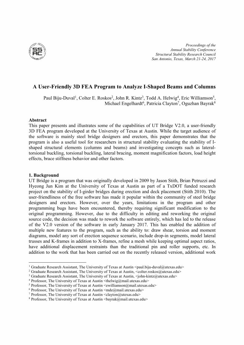
Proceedings of the Annual Stability Conference Structural Stability Research Council San Antonio, Texas, March 21-24, 2017 A User-Friendly 3D FEA Program to Analyze I-Shaped Beams and Columns Paul Biju-Duval 1 , Colter E. Roskos 2 , John R. Kintz 3 , Todd A. Helwig 4 , Eric Williamson 5 , Michael Engelhardt 6 , Patricia Clayton 7 , Oguzhan Bayrak 8 Abstract This paper presents and illustrates some of the capabilities of UT Bridge V2.0, a user-friendly 3D FEA program developed at the University of Texas at Austin. While the target audience of the software is mainly steel bridge designers and erectors, this paper demonstrates that the program is also a useful tool for researchers in structural stability evaluating the stability of I- shaped structural elements (columns and beams) and investigating concepts such as lateral- torsional buckling, torsional buckling, lateral bracing, moment magnification factors, load height effects, brace stiffness behavior and other factors. 1. Background UT Bridge is a program that was originally developed in 2009 by Jason Stith, Brian Petruzzi and Hyeong Jun Kim at the University of Texas at Austin as part of a TxDOT funded research project on the stability of I-girder bridges during erection and deck placement (Stith 2010). The user-friendliness of the free software has made it popular within the community of steel bridge designers and erectors. However, over the years, limitations in the program and other programming bugs have been encountered, thereby requiring significant modification to the original programming. However, due to the difficulty in editing and reworking the original source code, the decision was made to rework the software entirely, which has led to the release of the V2.0 version of the software in early January 2017. This has enabled the addition of multiple new features to the program, such as the ability to: draw shear, torsion and moment diagrams, model any sort of erection sequence scenario, include drop-in segments, model lateral trusses and K-frames in addition to X-frames, refine a mesh while keeping optimal aspect ratios, have additional displacement restraints than the traditional pin and roller supports, etc. In addition to the work that has been carried out on the recently released version, additional work 1 Graduate Research Assistant, The University of Texas at Austin <[email protected]> 2 Graduate Research Assistant, The University of Texas at Austin, <[email protected]> 3 Graduate Research Assistant, The University of Texas at Austin, <[email protected]> 4 Professor, The University of Texas at Austin <[email protected]> 5 Professor, The University of Texas at Austin <[email protected]> 6 Professor, The University of Texas at Austin <[email protected]> 7 Professor, The University of Texas at Austin <[email protected]> 8 Professor, The University of Texas at Austin <[email protected]>
-
Upload
khangminh22 -
Category
Documents
-
view
3 -
download
0
Transcript of A User-Friendly 3D FEA Program to Analyze I-Shaped Beams ...
Proceedings of the Annual Stability Conference
Structural Stability Research Council San Antonio, Texas, March 21-24, 2017
A User-Friendly 3D FEA Program to Analyze I-Shaped Beams and Columns
Paul Biju-Duval1, Colter E. Roskos2, John R. Kintz3, Todd A. Helwig4, Eric Williamson5, Michael Engelhardt6, Patricia Clayton7, Oguzhan Bayrak8
Abstract This paper presents and illustrates some of the capabilities of UT Bridge V2.0, a user-friendly 3D FEA program developed at the University of Texas at Austin. While the target audience of the software is mainly steel bridge designers and erectors, this paper demonstrates that the program is also a useful tool for researchers in structural stability evaluating the stability of I-shaped structural elements (columns and beams) and investigating concepts such as lateral-torsional buckling, torsional buckling, lateral bracing, moment magnification factors, load height effects, brace stiffness behavior and other factors. 1. Background UT Bridge is a program that was originally developed in 2009 by Jason Stith, Brian Petruzzi and Hyeong Jun Kim at the University of Texas at Austin as part of a TxDOT funded research project on the stability of I-girder bridges during erection and deck placement (Stith 2010). The user-friendliness of the free software has made it popular within the community of steel bridge designers and erectors. However, over the years, limitations in the program and other programming bugs have been encountered, thereby requiring significant modification to the original programming. However, due to the difficulty in editing and reworking the original source code, the decision was made to rework the software entirely, which has led to the release of the V2.0 version of the software in early January 2017. This has enabled the addition of multiple new features to the program, such as the ability to: draw shear, torsion and moment diagrams, model any sort of erection sequence scenario, include drop-in segments, model lateral trusses and K-frames in addition to X-frames, refine a mesh while keeping optimal aspect ratios, have additional displacement restraints than the traditional pin and roller supports, etc. In addition to the work that has been carried out on the recently released version, additional work
1 Graduate Research Assistant, The University of Texas at Austin <[email protected]> 2 Graduate Research Assistant, The University of Texas at Austin, <[email protected]> 3 Graduate Research Assistant, The University of Texas at Austin, <[email protected]> 4 Professor, The University of Texas at Austin <[email protected]> 5 Professor, The University of Texas at Austin <[email protected]> 6 Professor, The University of Texas at Austin <[email protected]> 7 Professor, The University of Texas at Austin <[email protected]> 8 Professor, The University of Texas at Austin <[email protected]>
2
continues on a number of other aspects, including the modeling of initial imperfections and the capability to perform a large displacement analysis on imperfect or curved systems. UT Bridge V2.0 was validated using theoretical solutions on simple systems as well as analyses on more complex scenarios using commercial software packages. In this paper, the focus is made on single straight structural elements in order to illustrate how useful the program may also be for researchers in structural stability, keeping in mind that analyzing complex bridge systems shall first be tested on simple structural elements. 2. Fundamentals The program uses an 8-noded isoparametric general shell element for all webs, flanges and transverse web stiffeners. A full 3D shell representation of the bridge is therefore provided, which offers a more accurate analysis of complex systems than the traditional 2D grid model considered by many commercial software packages (Zureick and Naqib 1999). Within the realm of 3D shell models, the approach considered is slightly different from a parallel approach where flanges are still modeled with beam elements instead. This is for example the case of BASP (Buckling Analysis of Stiffened Plates), a program developed in the 1970s to evaluate the stability of I-shaped structural elements. The behavior is essentially unchanged, but a full shell representation of an I-shaped structural element enables the capture of potential local buckling instabilities in the flanges. It also enables a more accurate definition of restraints and loads, for example warping restraints. Both approaches are considered accurate and state-of-the-art (NCHRP 725). The shell element mentioned above is well known for its accuracy and versatility (Bathe 1996). Since it is a quadratic element, it also fits well for curved systems. The drilling degree of freedom is not considered in the finite element formulation. Five degrees of freedom per node are retained. For nodes shared between flanges and webs, or webs and stiffeners, this results in six degrees of freedom overall. A reduced integration with four Gauss points is considered, with two integration layers through the shell thickness. This integration method was selected since full integration proved to produce excessively high stresses on curved systems with low radii of curvature, and also results in a higher computational cost. Extensive validation of the program on simple, as well as complex systems with severe skews or very low radii of curvature, was achieved by comparing the results against ABAQUS. In ABAQUS, the “S8R5” element is the finite element that is closest to the one discussed in the previous paragraph. One difference of the S8R5 is the use of a mixed interpolation for out-of-plane shear stresses. However, since the relative thickness of the shells with regards to their in-plane dimensions never gets particularly low for the models envisioned for the program, shear locking was proven not to be an issue. A mixed interpolation approach was therefore dismissed. From a programing perspective, modeling of a structure is achieved through a series of user-friendly Visual Basic forms, which leads to the generation of an input file that is then read and processed by a finite element program written in Fortran 90. Output files are then generated, which enables the 3D rendering of a structure, its deflected shape, moment and shear diagrams, and potential cross-frame forces in a viewer using some OpenGL functions.
3
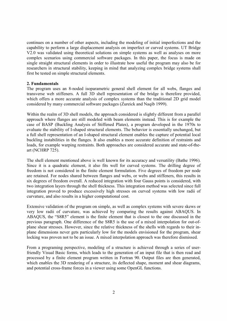
3. Case studies The following examples illustrate some of the basic capabilities of the program. 3.1 Case study #1: Deflections, reactions and moment diagrams In this first example, a 50’ long beam fixed at one end and supported at the other end loaded under its self-weight is considered. The cross-sectional dimensions are the following: 8”x1” for the top flange, 12”x1” for the bottom flange, and 40”x0.5” for the web. This is of course a simple problem. Yet, it is already a statically indeterminate system deflecting in double curvature, and the cross-section is singly-symmetric only. For this example, a fine mesh consisting of 8 elements through the web depth and 90 elements longitudinally was selected, resulting in a total of 17,575 degrees of freedom. The roller was modeled by restraining the vertical displacement at the bottom flange to web node, as well as the lateral displacement at both the bottom flange and top flange to web nodes. This is to prevent torsion and avoid rigid body instability modes while still permitting warping. On the other end, the fixity was modeled by additionally restraining the longitudinal displacement at both the bottom flange and top flange to web nodes (to prevent the rotation of the beam about its strong axis) and at all other flange nodes (to restrain warping of the flanges). The moment diagram is shown in Fig. 1. Note that it is automatically generated by the program. This is important for structural engineers working on advanced 3D FEA shell models. The finite element method indeed considers the displacements and rotations at all unrestrained degrees of freedom of a model as the main unknowns. However, structural engineers are often interested in other quantities as well such as the shear and moment diagrams. For shell models, commercial programs such as ABAQUS are unable to produce these diagrams and instead require a beam model. In that case however, the local behavior of a system is lost. Therefore, having the ability to produce those diagrams on a shell model is significant. It requires first the calculation of the location of the elastic neutral axis of the beam, and then the integration of the longitudinal stresses at all nodes across the section about that axis. For curved systems, the stresses are first converted to the local coordinate system of each point along the length the beam. In a similar way, shear is calculated at every point along the length of the beam by integrating the vertical shear stresses. For this example, the beam theory predicts a negative moment at the fixed end given by Eq. 1:
inkwLM 4.51082
min (1)
Whereas the maximum positive moment is given by Eq. 2:
inkwLM 1.2871289 2
max (2)
UT Bridge shows moments equal to – 490.7 k⸱in and + 295.4 k⸱in respectively (cf. Fig. 1), which means a relative difference of about – 3.9 % and + 2.9 %. This is fairly reasonable as stresses are
4
second derivatives of displacements, where some accuracy is inevitably lost in the post-processing of the displacements.
Figure 1: Moment diagram for a propped cantilever loaded under its self-weight only
Another basic capability of the program is to calculate the support reactions, which is useful for erectors worried about potential uplift. For curved systems, the restraints are transformed to the local coordinate system at the point considered, which means that radial boundary conditions are considered. In this example, the vertical reaction turns out to be equal to 4.27 kips at the fixed end and 2.62 kips at the roller end. Given the cross-sectional dimensions, the beam self-weight is calculated as 6.81 kips, equating to a relative difference of 1.2 % (without considering the extra weight provided by the fillets that would probably make up for some of that difference). If the “true” shell dimensions are considered instead, the overall self-weight of the beam becomes exactly 6.89 kips. The amplitude of the displacement vector at each node, as well as its three components, is derived at each node and able to be displayed in the viewer. In this example, the maximum deflection predicted by the beam theory is given by Eq. 3:
"30.01854
max EIwL (3)
where w is the self-weight of the beam (per unit length), E is the modulus of elasticity, I is the moment of inertia, and L is the length of the beam. UT Bridge provides the same value of 0.30”. Overall, UT Bridge accurately provides basic structural analysis calculations. Deflections, stresses (not shown here), reactions, moment, torsion and shear diagrams are available for use by
5
the bridge engineer. For curved systems, where bending and torsion are coupled, this is particularly significant. 3.2 Case study #2: Eigenvalue buckling analysis, Cb factors, load height effects In this second example, a 60’ long W30x90 is modeled using again 8 elements through the web depth. First, as in the previous example, only the self-weight of the beam is considered. The maximum deflection calculated by the program is equal to 0.25”, which corresponds to the beam theory solution given by Eq. 5:
"24.03845 4
max EIwL (5)
The same applies to the moment at mid-span, equal to 483.1 kips⸱in according the program, which compares well to the well-known expression given by Eq. 6:
inkwLM 6.48282
max (6)
A buckling analysis leads to a first eigenvalue equal to 3.73. This corresponds to a critical moment equal to 1802.2 kips⸱in. The original AISC equation originally derived by Timoshenko (Timoshenko and Gere 1961) for calculating the critical moment is given below as Eq. 7:
wybb
bcr CIL
EEIGJL
CM2
2
(7)
Where Cb is the moment magnification factor, Lb is the unbraced length, Iy is the moment of inertia about the weak axis and Cw is the torsional warping constant. In particular, Cb is given by Eq. 8 (AISC Specifications):
CBA
b MMMM
MC
3435.2
5.12
max
max (8)
Where Mmax is the maximum moment within the unbraced length, MA is the moment at quarter point of the unbraced length, MB is the moment at mid-span of the unbraced length, and MC is the moment at three-quarter point of the unbraced length. In this case, the critical moment ends up being equal to:
inkM cr
2.1866881,24114
720000,2957.2154,11114000,29
72014.1
22
6
This represents a relative difference of 3.4%. In addition to validating Eq. 7, UT Bridge is also a tool to back-calculate Cb factors, which were themselves initially derived by similar programs such as BASP (Akay, Johnson and Will 1977). Here for example, the moment magnification factor for a parabolic moment distribution within the unbraced length would be equal to:
10.1)14.1/2.1866(2.1802 bC
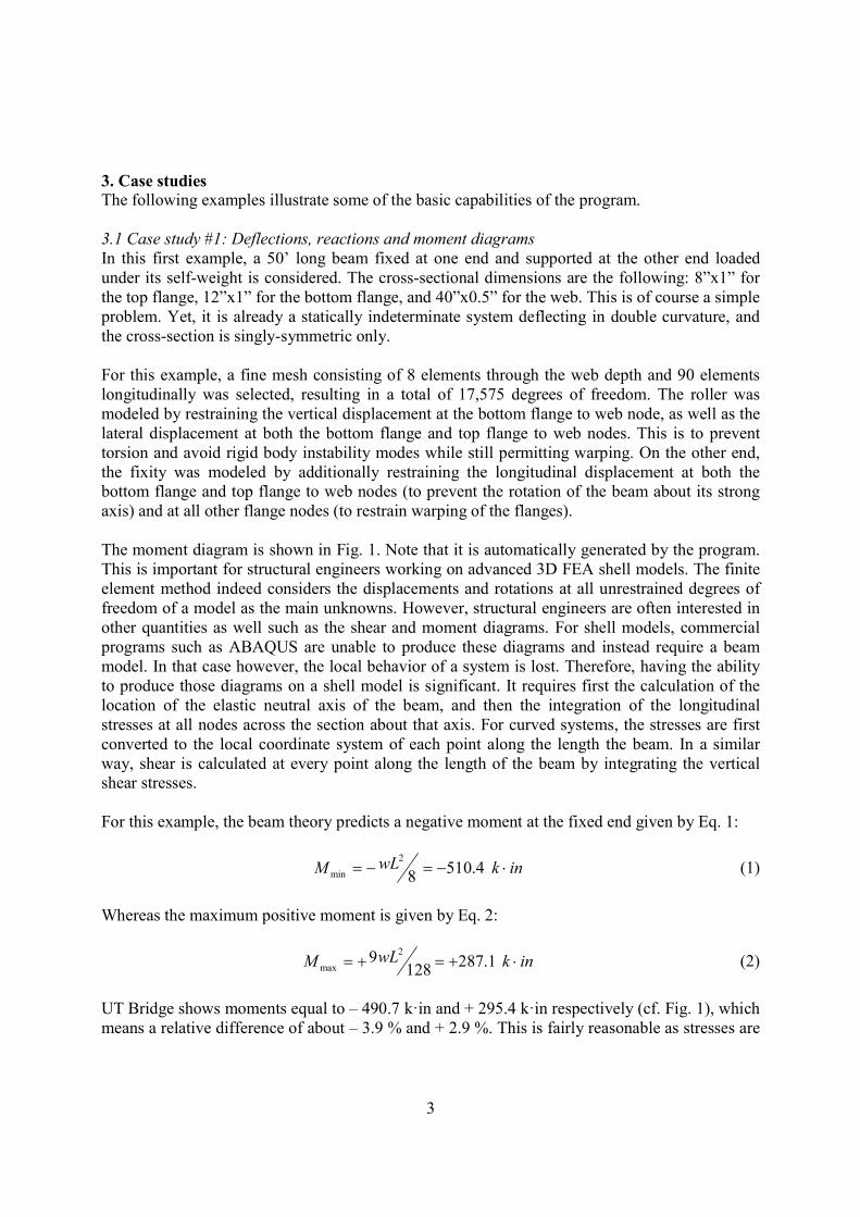
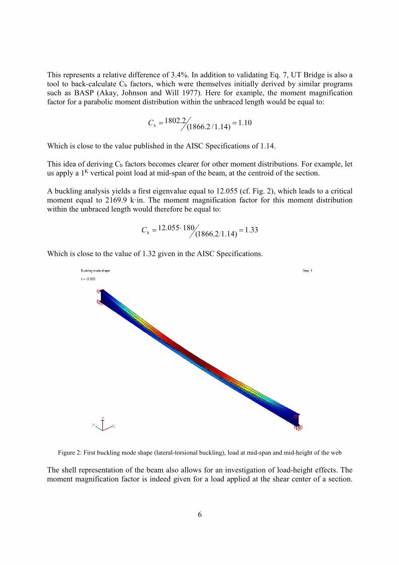
Which is close to the value published in the AISC Specifications of 1.14. This idea of deriving Cb factors becomes clearer for other moment distributions. For example, let us apply a 1K vertical point load at mid-span of the beam, at the centroid of the section. A buckling analysis yields a first eigenvalue equal to 12.055 (cf. Fig. 2), which leads to a critical moment equal to 2169.9 k⸱in. The moment magnification factor for this moment distribution within the unbraced length would therefore be equal to:
33.1)14.12.1866(180055.12 bC
Which is close to the value of 1.32 given in the AISC Specifications.
Figure 2: First buckling mode shape (lateral-torsional buckling), load at mid-span and mid-height of the web
The shell representation of the beam also allows for an investigation of load-height effects. The moment magnification factor is indeed given for a load applied at the shear center of a section.
7
However, for a load applied at a different height through the web, a modifying factor must be applied (Helwig, Frank and Yura 1997), which is given in Eq. 10: hy24.1 (10) Where h is the depth of the web, and y is the vertical coordinate of the node where the point load is applied (+0.5h for the bottom flange to web node, -0.5h for the top flange to web node). The point load was therefore applied at different locations through the depth of the web. The results are given as follows, where λ denotes the eigenvalue corresponding to the first buckling mode:
73.083.8
85.030.10
18.122.14
39.171.16
4/2/
4/4/
4/4/
2/2/
hyhy
hyhy
hyhy
hyhy
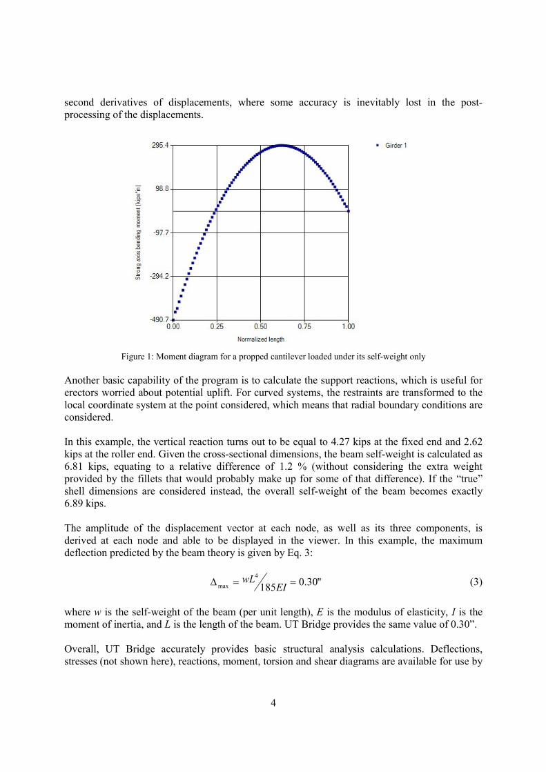
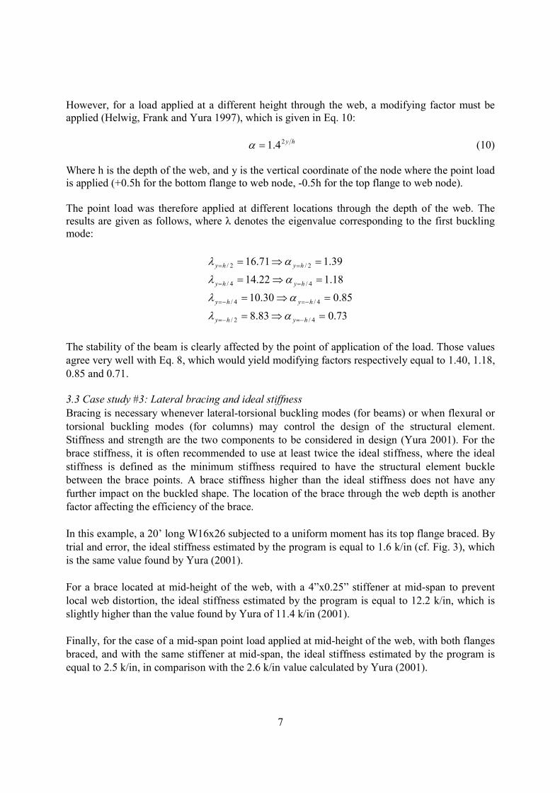
The stability of the beam is clearly affected by the point of application of the load. Those values agree very well with Eq. 8, which would yield modifying factors respectively equal to 1.40, 1.18, 0.85 and 0.71. 3.3 Case study #3: Lateral bracing and ideal stiffness Bracing is necessary whenever lateral-torsional buckling modes (for beams) or when flexural or torsional buckling modes (for columns) may control the design of the structural element. Stiffness and strength are the two components to be considered in design (Yura 2001). For the brace stiffness, it is often recommended to use at least twice the ideal stiffness, where the ideal stiffness is defined as the minimum stiffness required to have the structural element buckle between the brace points. A brace stiffness higher than the ideal stiffness does not have any further impact on the buckled shape. The location of the brace through the web depth is another factor affecting the efficiency of the brace. In this example, a 20’ long W16x26 subjected to a uniform moment has its top flange braced. By trial and error, the ideal stiffness estimated by the program is equal to 1.6 k/in (cf. Fig. 3), which is the same value found by Yura (2001). For a brace located at mid-height of the web, with a 4”x0.25” stiffener at mid-span to prevent local web distortion, the ideal stiffness estimated by the program is equal to 12.2 k/in, which is slightly higher than the value found by Yura of 11.4 k/in (2001). Finally, for the case of a mid-span point load applied at mid-height of the web, with both flanges braced, and with the same stiffener at mid-span, the ideal stiffness estimated by the program is equal to 2.5 k/in, in comparison with the 2.6 k/in value calculated by Yura (2001).
8
UT Bridge is therefore very capable of estimating an ideal brace stiffness for different moment distributions and brace configurations.
Figure 3: First buckling mode shape (uniform moment distribution, top flange bracing, brace stiffness higher than
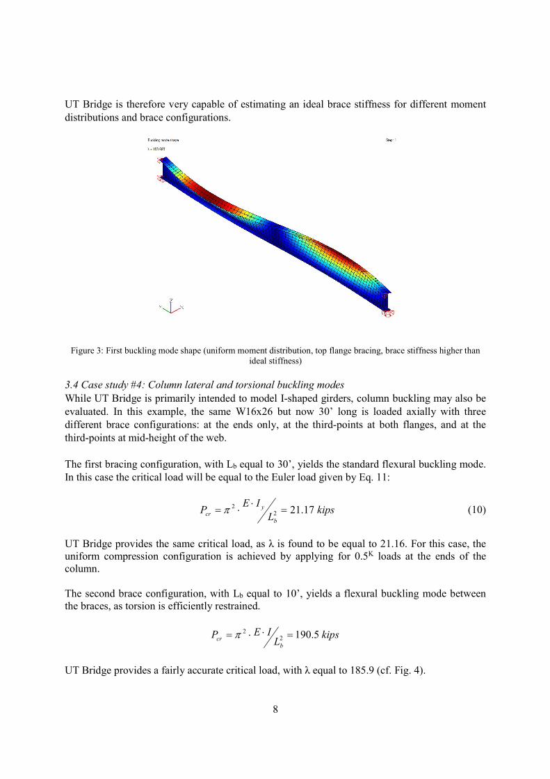
ideal stiffness) 3.4 Case study #4: Column lateral and torsional buckling modes While UT Bridge is primarily intended to model I-shaped girders, column buckling may also be evaluated. In this example, the same W16x26 but now 30’ long is loaded axially with three different brace configurations: at the ends only, at the third-points at both flanges, and at the third-points at mid-height of the web. The first bracing configuration, with Lb equal to 30’, yields the standard flexural buckling mode. In this case the critical load will be equal to the Euler load given by Eq. 11:
kipsL
IEP
b
ycr 17.212
2
(10)
UT Bridge provides the same critical load, as λ is found to be equal to 21.16. For this case, the uniform compression configuration is achieved by applying for 0.5K loads at the ends of the column. The second brace configuration, with Lb equal to 10’, yields a flexural buckling mode between the braces, as torsion is efficiently restrained.
kipsL
IEPb
cr 5.19022
UT Bridge provides a fairly accurate critical load, with λ equal to 185.9 (cf. Fig. 4).
9
Figure 4: Column first buckling mode, intermediate bracing at the third points at both flanges
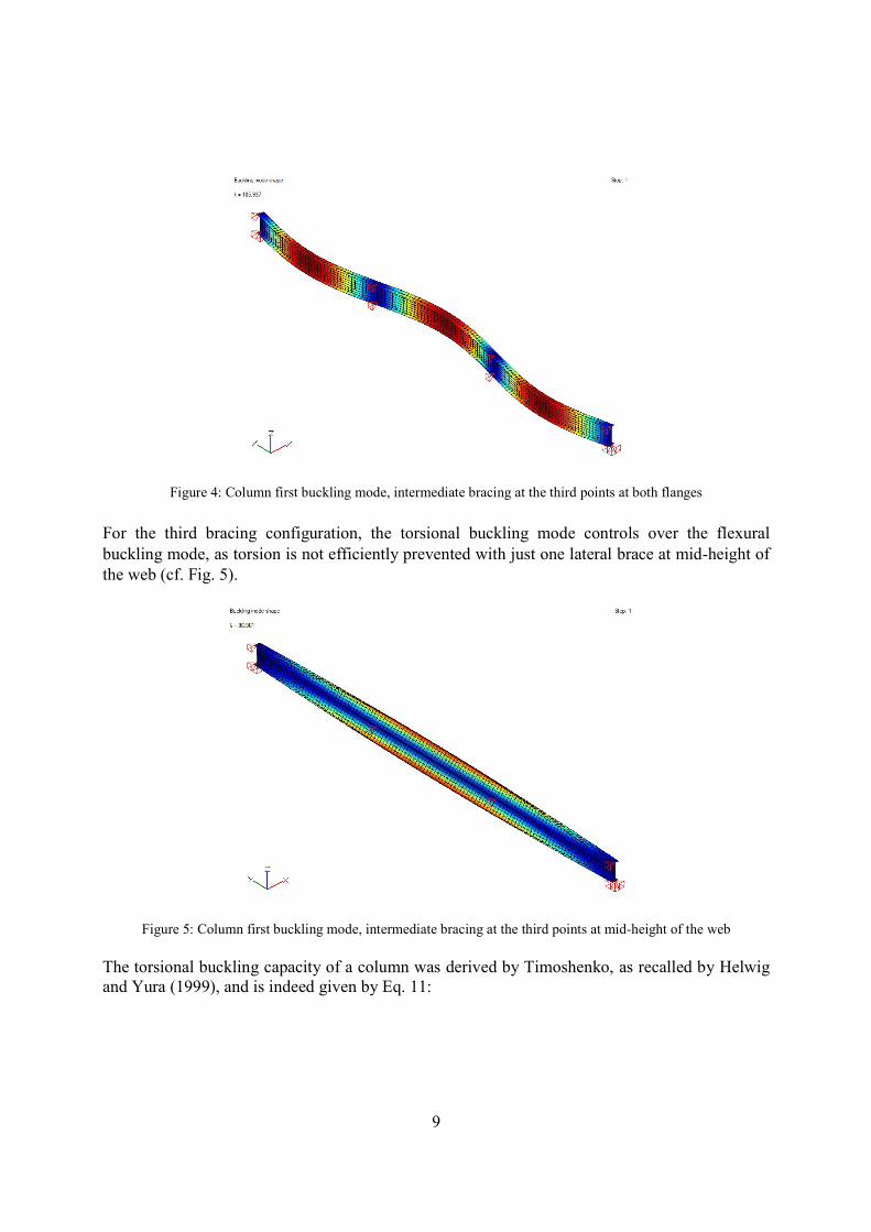
For the third bracing configuration, the torsional buckling mode controls over the flexural buckling mode, as torsion is not efficiently prevented with just one lateral brace at mid-height of the web (cf. Fig. 5).
Figure 5: Column first buckling mode, intermediate bracing at the third points at mid-height of the web
The torsional buckling capacity of a column was derived by Timoshenko, as recalled by Helwig and Yura (1999), and is indeed given by Eq. 11:
10
22
2)4(
yx
ey
Trr
JGdPP
(11)
Where rx and ry are the strong and weak radii of gyration respectively, d is the distance between the flange centroids, and Pey is the elastic flexural buckling load based on the column length between points of zero twist, given by Eq. 12:
2
2
T
yey L
IEP
(12)
Where LT is the unbraced length for torsion. In this case, we have:
kipsPey 17.21
kipsPT 4.9413.124.6
229.0111544
345.1517.21
22
2
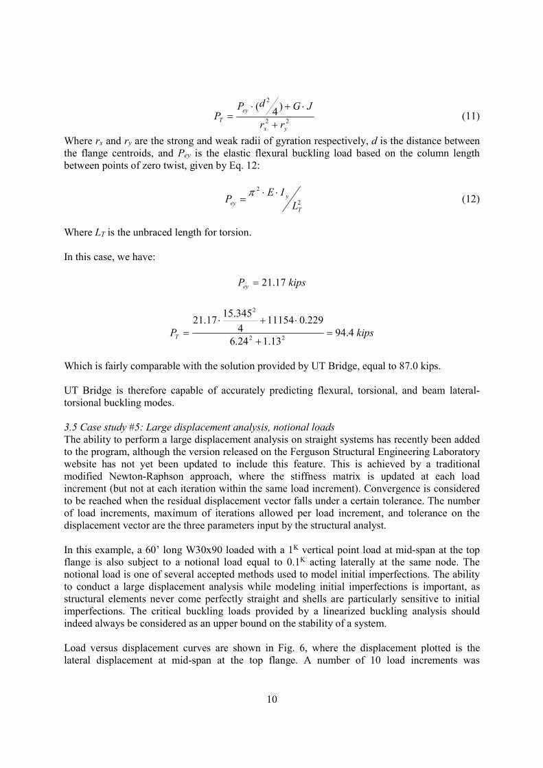
Which is fairly comparable with the solution provided by UT Bridge, equal to 87.0 kips. UT Bridge is therefore capable of accurately predicting flexural, torsional, and beam lateral-torsional buckling modes. 3.5 Case study #5: Large displacement analysis, notional loads The ability to perform a large displacement analysis on straight systems has recently been added to the program, although the version released on the Ferguson Structural Engineering Laboratory website has not yet been updated to include this feature. This is achieved by a traditional modified Newton-Raphson approach, where the stiffness matrix is updated at each load increment (but not at each iteration within the same load increment). Convergence is considered to be reached when the residual displacement vector falls under a certain tolerance. The number of load increments, maximum of iterations allowed per load increment, and tolerance on the displacement vector are the three parameters input by the structural analyst. In this example, a 60’ long W30x90 loaded with a 1K vertical point load at mid-span at the top flange is also subject to a notional load equal to 0.1K acting laterally at the same node. The notional load is one of several accepted methods used to model initial imperfections. The ability to conduct a large displacement analysis while modeling initial imperfections is important, as structural elements never come perfectly straight and shells are particularly sensitive to initial imperfections. The critical buckling loads provided by a linearized buckling analysis should indeed always be considered as an upper bound on the stability of a system. Load versus displacement curves are shown in Fig. 6, where the displacement plotted is the lateral displacement at mid-span at the top flange. A number of 10 load increments was
11
considered. The lateral displacement at mid-span turns out to be 8.3% higher when using a large displacement analysis, which is significant for a notional load of only 0.1K, but is comparable with the same analysis conducted on ABAQUS.
Figure 6: Load versus displacement curves (lateral displacement at mid-span, top flange)
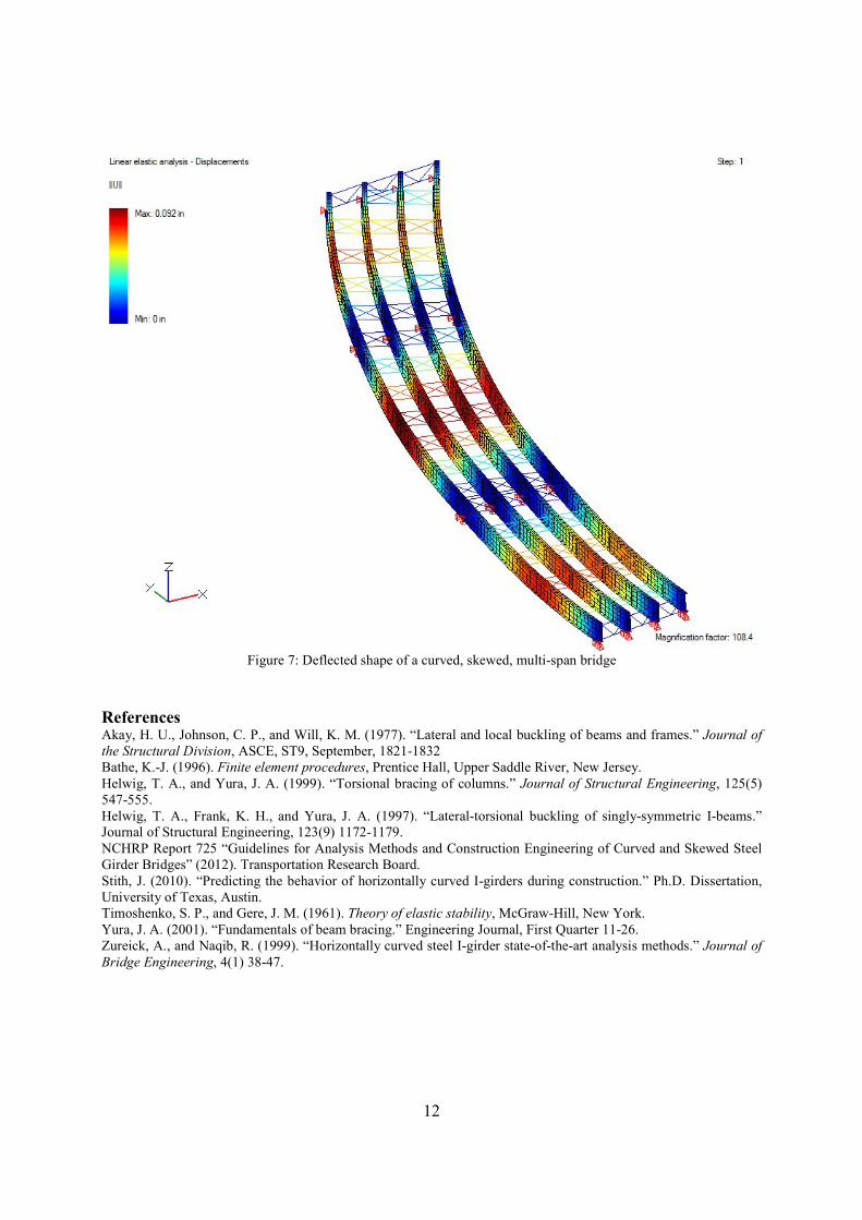
4. Conclusions This paper briefly presented how UT Bridge, a 3D FEA program used by steel bridge engineers and erectors to analyze curved I-girder bridges during erection and deck placement, can also be a useful tool for researchers in structural stability investigating the buckling of I-shaped beams and columns. Many of the equations included in the Stability chapter of the AISC Specifications were actually derived or verified with BASP, which was developed in the late 1970s and has not gone through any significant update in the past decade. UT Bridge includes the capabilities of BASP, but is also able to model much larger systems (cf. Fig. 7), including curved and skewed multi-span non-prismatic systems. UT Bridge provides a conventional structural analysis in addition to the buckling analysis available by using BASP, and generates a clear visual rendering of the structures and their deflected shapes. Future developments for the program include the ability to perform a large displacement analysis on curved systems, as well as the ability to model different types of initial imperfections not only by adding notional loads but by actually modifying the initial geometry of the structures. Other types of bridges, such as tub girder bridges, are also planned to be covered by the program in the future. Acknowledgements The authors would like to thank the Texas Department of Transportation for funding of this project. The opinions presented in this paper are those of the authors and do not necessarily reflect the views of the sponsor.
12
Figure 7: Deflected shape of a curved, skewed, multi-span bridge
References Akay, H. U., Johnson, C. P., and Will, K. M. (1977). “Lateral and local buckling of beams and frames.” Journal of the Structural Division, ASCE, ST9, September, 1821-1832 Bathe, K.-J. (1996). Finite element procedures, Prentice Hall, Upper Saddle River, New Jersey. Helwig, T. A., and Yura, J. A. (1999). “Torsional bracing of columns.” Journal of Structural Engineering, 125(5) 547-555. Helwig, T. A., Frank, K. H., and Yura, J. A. (1997). “Lateral-torsional buckling of singly-symmetric I-beams.” Journal of Structural Engineering, 123(9) 1172-1179. NCHRP Report 725 “Guidelines for Analysis Methods and Construction Engineering of Curved and Skewed Steel Girder Bridges” (2012). Transportation Research Board. Stith, J. (2010). “Predicting the behavior of horizontally curved I-girders during construction.” Ph.D. Dissertation, University of Texas, Austin. Timoshenko, S. P., and Gere, J. M. (1961). Theory of elastic stability, McGraw-Hill, New York. Yura, J. A. (2001). “Fundamentals of beam bracing.” Engineering Journal, First Quarter 11-26. Zureick, A., and Naqib, R. (1999). “Horizontally curved steel I-girder state-of-the-art analysis methods.” Journal of Bridge Engineering, 4(1) 38-47.