A unified framework for estimating or updating origin/destination matrices from traffic counts

Tronrpn. Res:B. Vol 228. No 6. pp 437-J%. 19HX Prmred m Great Bruin.

0191.?615iSR 13 CO+ .OlJ ‘C 1988 Pergamon Press plc

A UNIFIED FRAMEWORK FOR ESTIMATING OR UPDATING ORIGIN/DESTINATION MATRICES FROM

TRAFFIC COUNTS

ENNIO CASCETTA Istituto di Tecnica ed Economia dei Trasporti. Universita di Napoli, Napoli. Italia

and

SANG NGUYEN Departement d’informatique et de recherche operationnelle et Centre de Recherche sur les

Transports, Universite de Montreal. Canada

(Received 8 December 1986; in revised form 30 December 1987)

Abstract-This paper presents an in-depth study of the methodology for estimating or updating origin-to-destination trip matrices from traffic counts. Following an analysis of the statistical foundation of the estimation and updating problems. various basic approaches are reviewed using a generic traffic assignment map. Computational issues related to specific assignment maps and estimation models for both road and transit networks are then discussed. Finally, additional insight into the relative performance of several estimators is provided by a set of test problems with varying input data.

1. INTRODUCTION

Consider a transport network, abstracted into a graph model, consisting of a set. I ‘of nodes and a set 1 of directed links (arcs). A node at which trips originate and/or terminate is called a centroid. Let rrS denote the average number of trips going from centroid r to centroid S, within a given time period. Let T be a vector? with components t,*. T is usually referred to as an origin-destination trip matrix.

Each origin-destination flow t,S subdivides on the network into path flows y,sk, k E

I,J, where I, is a subset of all paths connecting the pair of centroids r and S. For a given link I E 1, the sum of all path flows traversing this link is denoted by

the link flow u/:

u/ = 2 2 hkyrrk,

n kEl,

(1.1)

where 8/k equals 1 if path k traverses link I and 0 otherwise. In a more compact notation, eqn (1.1) may be rewritten as

v = AY, (1.2)

where A is the usual multi-origin-destination pairs link-path incidence matrix, and V and Y are, respectively, vectors of link and path flows.

With every arc 1 E 1 is associated an average unit travel cost c,(V), which may be a fixed constant or a function of link flow V. In addition, to reflect the variation and error in the trip maker’s perception of travel costs-both across the trip maker population and time-the perceived travel cost C,(V) is considered to be a random variable with mean value c,(V):

E,(V) = c,(V) + E/. (1.3)

tAll vectors are column vectors: ’ denotes transposition.

137

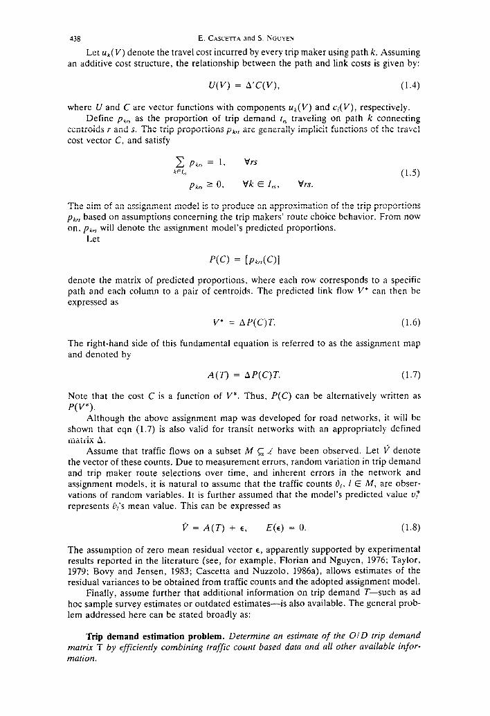
438 E. CASCEITA and S. NGUYEY

Let Us denote the travel cost incurred by every trip maker using path k. Assuming an additive cost structure, the relationship between the path and link costs is given by:

U(V) = A’C(V), (1.4)

where I/ and C are vector functions with components uJV> and c,(V), respectively. Define pkrJ as the proportion of trip demand t, traveling on path k connecting

centroids r and S. The trip proportions p k,s are generally implicit functions of the travel cost vector C, and satisfy

c pkn = I. Vrs kEl,< (1.5)

pkrr z 0, Vk E I,, tlrs.

The aim of an assignment model is to produce an approximation of the trip proportions pkls based on assumptions concerning the trip makers’ route choice behavior. From now on, pk,* will denote the assignment model’s predicted proportions.

Let

p(c> = [Pkrs(C)l

denote the matrix of predicted proportions, where each row corresponds to a specific path and each column to a pair of centroids. The predicted link flow V* can then be expressed as

V* = AP(C)T. (1.6)

The right-hand side of this fundamental equation is referred to as the assignment map and denoted by

A(T) = AP(C)T. (1.7)

Note that the cost C is a function of V*. Thus, Z’(C) can be alternatively written as P( v*).

Although the above assignment map was developed for road networks, it will be shown that eqn (1.7) is also valid for transit networks with an appropriately defined matrix A.

Assume that traffic flows on a subset M c 1 have been observed. Let V denote the vector of these counts. Due to measurement errors, random variation in trip demand and trip maker route selections over time, and inherent errors in the network and assignment models, it is natural to assume that the traffic counts O,, 1 E M, are observations of random variables. It is further assumed that the model’s predicted value u; represents ii,‘s mean value. This can be expressed as

V = A(T) + E, E(E) = 0. (1.8)

The assumption of zero mean residual vector E, apparently supported by experimental results reported in the literature (see, for example, Florian and Nguyen, 1976; Taylor, 1979; Bovy and Jensen, 1983; Cascetta and Nuzzolo, 1986a), allows estimates of the residual variances to be obtained from traffic counts and the adopted assignment model.

Finally, assume further that additional information on trip demand T-such as ad hoc sample survey estimates or outdated estimates -is also available. The general problem addressed here can be stated broadly as:

Trip demand estimation problem. Determine an estimate of the OID trip demand matrix T by efficiently combining traffic count based data and all other available information.

Estimating or updating origin/destination matrices 439

Depending on the nature of the available information, the above problem may be formulated differently. For instance, if sample survey estimates are given, the estimation problem can be seen as that of attempting to combine two distinct sets of experimental data (survey estimates and traffic counts), related to the unknown trip demand T.

On the other hand, if an a priori probability distribution of T-formalizing our subjective knowledge about the demand T-is given, then the estimation problem will reduce to that of attempting to combine a priori information and experimental data.

This article provides a unified framework for the estimation or the updating of a trip matrix T from traffic counts, for both car and transit networks. Section 2 shows that both the classical and the Bayesian inference techniques, in addition to the standard minimum information (maximum entropy) approach, may be used to develop choice criteria for trip demand estimates. For each approach, a generic optimization formulation for the estimation problem, using an abstract traffic assignment map A(T) is then described. Computational issues related to the assignment map, as well as, the estimation problem are addressed in Section 3. A small illustrative numerical example is described in the last section.

This paper differs from an earlier survey of models and methods for car networks given by Nguyen (1984) in several aspects. First, by placing emphasis on the conventional statistical inference methods rather than on the traditional entropy-maximizing approach used in the transportation field (Wilson, 1970), it provides a larger variety of trip matrix estimators, and new insight into the trip matrix estimation problem. And second, by introducing a model independent assignment map, it presents a unified framework for car and transit networks which has not been described previously.

2. FORMULATIONS OF THE ESTIMATION PROBLEbl

This section formulates trip matrix estimation or updating as optimization problems. The objective function of the latter depends on the statistical inference techniques adopted. Within the classical inference approach, the maximum likelihood (ML) and the generalized least-squares (GLS) methods for deriving objective functions will be examined, and contrasted to the Bayesian method. The different approaches considered in this section are related to methods proposed previously by various researchers, such as Landau er al. (1982), Maher (1983), Spiess (1983a), Cascetta (1984), McNeil (1983), and Ben-Akiva et al. (198.5), among others. The maximum entropy models (see, for example, Wilson, 1970; Snickars and Weibull, 1977; Van Zuylen and Willumsen, 1980; Nguyen, 1983) will not be reviewed here, as they were described in detail in Nguyen (1984). However, the relationship between these and certain Bayesian models will be pointed out.

2.1 ML estimators ML estimators are obtained by maximizing the likelihood of observing the experi-

mental data conditional on the true trip matrix T. The data consists of a set of sample counts u,~ with given sampling fractions 01, used

in the survey, and a set of traffic counts 5,. These two sets of data are usually considered to be statistically independent, so the likelihood of observing both sets can be expressed as

l(N, V’IT) = l(A’IT) . /(PIT). (2-l)

The maximum likelihood estimator TbfL of trip demand T may then be obtained by maximizing expression (2.1) or, more conveniently, its natural logarithm:

plL = arg tn~;{ln .t(iVIT) + lnI(PIT)}, (2.2)

where S is the set of feasible T. Unless explicitly specified, S will simply be the set of all nonnegative T.

440 E. CASCETTA and S. NGCYEN

The computation of T,ML will depend on the probability distribution assumed for the effective sample count vector N and that of the traffic count vector p (or equivalently the residual E in eqn (1.8)). In practice, the muftivariare normal (MVN) and the Poisson are perhaps the prevailing distribution choices for the error E.

If the traffic counts are independent Poisson variates with means u; = A(T), (Van Zuylen and Branston, 1982), then

In I(PIT) = c [it, In A(T), - A(T),] + constant. /EM

(2.3)

On the other hand, if the error terms are assumed to have a joint MVN distribution with zero mean and an arbitrary variance-covariance matrix W (Maher, 1983; Cascetta, 1984, 1986), then

In _L(PIT) = -&(P - A(T))‘W-’ (i/ - A(T)) + constant. (2.4)

Although traffic counts are discrete random variables that take only positive values, the MVN error distribution assumption is not totally inappropriate, since given the usual level of measured flows and error variances, the probability of obtaining a negative value is practically negligible. Possible ways for estimating the error variances are outlined in Section 3.

The distribution of the sample count vector N depends naturally on the sampling procedure adopted (e.g., simple random, stratified, or cluster sampling). Only the simple random sampling is considered here.

If II, out of r,. trips are sampled at each origin r, and if the sampling fractions

a, = n,it,, are sufficiently low, then sample N may be assumed to follow a multinomial distribution so that

where

In this case,

lnJ(NIT) = C n,x ln(o,t_) + constant, ,S

(24

and the constraint set S becomes:

If the number of trips sampled at each origin and the number of possible destinations are sufficiently large, then the likelihood function 1 (NIT) may be expressed as a product of Poisson probability functions with parameters a,t,3:

(2.7)

leading to

Estimating or updating originidestination matrices 441

In J(N(T) = 2 [n, ln((~,t,~) - CY,~~] + constant. n

(2.8)

In summary, the objective function in optimization problem (2.2) is the sum of (2.6) or (2.8) and either (2.3) or (2.4). The computational complexity of model (2.2) depends largely on the assignment map A(T).

Note that (2.4) may be considered alternatively as a penalty function for the deterministic constraint

A(T) = P,

which corresponds to the limiting case where the variances of the error terms are set to zero.

Finally, note that T”L- the ML estimators-are asymptotically consistent, efficient, and normally distributed: TML - MVN(T, W,,,) with mean T and dispersion matrix

-’ w,,, = - )I . (2.9)

For large samples, this dispersion matrix can be approximated by the negative inverse of the Hessian of In J(N, VIT) evaluated at T ‘IL Also, by substituting In J(N, p’(T) . in expression (2.9) by the sum of In I(NIT) and In 1(p/T), one can see that the T’IL estimator variances are lower than those of an ML estimator based solely on sample counts.

2.2 GLS estimator The advantage of this approach is that no distributional assumptions must be made

on the sets of data. Let ii- denote the survey estimate of T obtained from grossing up the sample counts, independently of the sampling technique used. Consider the following stochastic system of equations in T:

i”=T+q

v = A(T) + E, (2.10)

in which q is the sampling error with a variance-covariance matrix Z, and E is the traffic count error with dispersion matrix W introduced earlier. The GLS estimator TCLS of T may then be obtained by solving:

TCLS = arg min(? - T)‘Z-‘(f - T) + (p - A(T))‘W-‘(v - A(T)). (2.11) TES

The estimation of dispersion matrix Z depends on the sampling scheme adopted. For origin-based simple random sampling with sufficiently small sampling fractions, Z can be approximated as follows:

Var(i,) = $ 1. ( )

I-F 1.

Cov(i,, irk) = - F r.

Cov(i,, i(k) = 0.

142 E. CASCETTA and S. NGL’YEN

Note that the GLS estimator (2.11) coincides with the ML estimator when MVN distributions are assumed for both N and v. For assignment models that produce a linear map A(T) = AT, under certain simplifying assumptions, TCLS can be shown to be an unbiased most efficient linear estimator, and its dispersion matrix W,,, can be related to that of ? as follows:

W GLS = Z - ZA’(W + AZA’)-‘AZ. (2.12)

The above expression also shows that a reduction of variance is obtained by combining survey data with traffic count based information, since the second term on the right- hand side of eqn (2.12) corresponds to a positive (semi) definite matrix (Judge et al., 1980).

2.3 The Bayesian approach

In the Bayesian inference framework, a priori information on the trip demand T is expressed as a prior probability function g(T), the parameters of which are a function of the a priori estimates q_ of the unknown t,,. The qr5 are either rough or obsolete estimates, or estimates resulting from a combination of several distinct data sets.

On the other hand, the traffic counts represent an additional source of information about T with given probability /(PIT); Bayes theorem allows these two sources of information to be combined to provide the posterior probability function f(T/P) (i.e.. the probability of observing T conditional to the traffic count P):

W-t@ x @IT) . g(T). (2.13)

In principle, the above posterior probability function allows a confidence region to be generated for T. In practice, due to computational complications, only point estimators can be obtained, either as the posterior expected value:

TB = E(TIp) = Tf( T/v) dT, (2.14)

or as the maximum value of (the logarithm of) the posterior distribution (the mode of the posterior distribution):

TB = arg in:.; In f(Tli’). (2.15)

The maximum posterior distribution estimator is a substitution for the expected value, when this latter requires complex numerical integration.

If multivariate normal or independent Poisson distributions are assumed for the traffic counts, then the likelihood function .l(plT) is given by either (2.3) or (2.4). On the other hand, the most frequently used prior distribution g(T) is the multinomial distribution, which provides a simple analytical log-function.

Indeed, if the prior distribution g(T) is a multinomial with probabilities proportional to the a priori estimates q,5:

g(T) = (2.16)

where q.. = I& q,3. then using Stirling’s approximation for the logarithm of factorial terms yields

In g(T) = - c t,5 In ;s + constant, ,S

(2.17)

Estimating or updating origin/destination matrices

where the total number of trips is assumed fixed:

443

2 f, = constant. r*

The above function (2.17) is identical to Kullback’s discriminatoryfunction or the entropy function of T (Kullback, 1959), which pervades maximum entropy models in transportation and regional planning (see, for example, Wilson, 1970; Snickars and Weibull, 1977; Van Zuylen and Willumsen, 1980; Nguyen, 1983). In particular, the generic maximum entropy trip matrix estimation problem can be formulated as follows:

TE = argmax - c t,ln:, TES TX IS

(2.18)

where the set S of feasible T is here defined as:

A(T) = Q

c t, = constant IS

Ts 0. (2.19)

This formulation can be seen as a particular instance of problem (2.15), when the objective is the sum of (2.4) and (2.17).

With Poisson approximation to the multinomial distribution:

the log-function becomes

ln g(T) = -2 t, 0

(In ; - I) + constant,

(2.20)

(2.21)

which again may also be obtained from the maximum entropy principle. Less frequently used is a multivariate normal prior distribution, with mean Q and

dispersion matrix W, (Maher, 1983):

g(T) 3~ exp( -1(T - Q)‘Wa’(T - Q)),

yielding

In g(T) = - +(T - Q)' W;‘(T - Q) + constant. (2.22)

In summary, a Bayesian estimator of T may be obtained by solving the optimization problem (2.14), the objective function of which is a sum of two log-functions. Under different assumptions, the log-function associated with traffic counts is either function (2.3) or (2.4); and that related to the prior distribution is either function (2.16), (2.17). (2.21) or (2.22). Note that expressions for the variance-covariance matrix of Bayesian estimators can also be developed. However, in the present case, variances and covari- antes of the estimators are only measures of the subjective uncertainty posterior to the use of traffic counts.

So far, it has been assumed that the experimental information on T is given uniquely by the set of traffic counts. If survey data are also available, they can be used simulta-

44-t E. C~\SCETTA and S. NGUYEN

neously with traffic counts to yield the following posterior probability:

so that

T* = arg t-n;; [In J(VlT) + In /(NIT) + In g(T)].

All functions /(NIT), developed earlier, can be used in the above objective function. It is perhaps worth noting the different roles assumed by Tin the classical and the

Bayesian inference approach. In the first case, the true t,5 are parameters of the sampling likelihood function 1 (N(T), and in the second case the rrX are random variables with given prior distributions.

3. COMPUTATIONAL CONSIDERATIONS

This section addresses the statistical issues related to the collection of traffic counts, to the choice of traffic count distributions, as well as to the count-independent information (i.e., survey or a priori trip matrix), and discusses the computation of existing assignment maps for both road and transit networks.

3.1 Statistical aspects Links with fraffic count. From the variance reduction property obtained with the

generalized least squares approach (see expression (2.12) describing the GLS dispersion matrix), it follows that to maximize the expected variance reduction, the counted links should have the lowest possible variance to mean ratios and should have uncorrelated or negatively correlated residuals. Hence, in practice, links with large flows along a screen line should be chosen. Finally, the larger the number of links with similar char- acteristics included in the traffic count data set, the larger will be the variance reduction obtained.

Traffic count distributions. As mentioned in Section 2, the multivariate normal and the Poisson distributions are the major distributions used in practice. For data sets with large counts (say larger than 500 veh/hour), the normal distribution seems to be pref- erable to the Poisson distribution for the following reasons. First, the normal distribution allows different variances to be used for links with the same level of flow. Experimental studies, reported in the literature, provide a means of estimating these error variances using essentially the sample standard deviation. Second, if links are chosen appropriately, the error covariances can be ignored on a first approximation, so that the dispersion matrix W in eqn (2.4) reduces to a diagonal matrix. This generally decreases the effort required to solve the estimation problem.

In addition, there is a certain flexibility in the use of traffic counts, since in the limit. setting the variances of the errors to zero amounts to imposing the deterministic constraint: A(T) = P in the estimation problem. However, if errors are actually present in the counts and the survey based information is reasonably accurate, it is possible to produce an increase in the mean squared errors by imposing the above deterministic constraint. On the other hand, dealing with constraints rather than probability distribution functions directly may allow the development of simpler and more consistent models.

Count independent information. Count independent information on the true trip demand matrix is often biased and underestimated. For survey estimates, this under- estimation results from the well-known trip understatement phenomenon, whereas for a priori information based on outdated demand, this comes usually from an increase in total demand. In this case, the decrease in the mean squared errors, obtained with the traffic count data set, is more significant the larger the starting estimate bias, as shown by the simulation results in Section 4.


A problem that is worth mentioning is that caused by zero cell entries in the survey or a priori estimates in the Bayesian inference approach. The cells with zero counts cannot have positive estimated values with multinomiai and Poisson prior distributions- an undesirable feature. In general, a certain “seeding” of zero cell entries must be adopted.

Trip demand estimator. In the classical inference framework, the ML is superior to the GLS estimator for large samples. However, this theoretical superiority vanishes for finite samples, and indeed experiments confirm this (Cascetta, 1984). Note also that a closed functional form of the loglikelihood of sample count N may not be easily obtained, except for certain sampling schemes (simple multinomial or Poisson sampling). In this respect, the GLS estimator has the advantage of being independent of the sampling distribution.

GLS estimation requires the calculation of the covariance matrix Z of T. In practice, a diagonal matrix is frequently used to diminish the computational effort required in solving the estimation problem. Estimates of the variances of i,s can be obtained for the majority of sampling schemes (see, for instance, Yates, 1981).

The MVN prior distribution (2.22) has the undesirable feature of allowing negative estimated values. On the other hand, it permits different subjective confidences to be placed on various trip matrix cells by tailoring appropriately the corresponding cell variances in the dispersion matrix W,.

3.2 Computing assignment maps Existing assignment models are built on the premise that every trip maker, being

a rational decision maker, minimizes his or her perceived journey cost in the choice of routing alternative. An alternative either represents a single path in road networks or a collection of paths with fixed path probabilities-called a hyperpath in transit networks (Nguyen and Pallottino, 1985a). The notion of hyperpath will be detailed shortly.

The average link cost-travel time or generalized travel cost-can be considered as a flow independent constant in uncongested networks or as a first approximation in congested networks, but more realistically it is a function of traffic flow. Independently from the functional form given to the average cost, if it is assumed that trip makers are identical and possess perfect knowledge of the network and the travel costs incurred on the network, we obtain the class of deterministic assignment models in which the user’s perceived cost is exactly the average cost. For instance, when travel costs are assumed to be flow independent constants, only a single alternative is utilized between each pair of centroids, giving rise to “all-or-nothing” assignment models; when the average travel cost increases with flows-in congested urban networks-then multiple alternatives with equal minimum travel costs are utilized between each pair of centroids, leading to Wardrop equilibrium-based models (Wardrop, 1952).

On the other hand, stochastic assignment models take into account the variation and error in the trip maker’s perception of travel costs. Consequently, multiple alternatives are utilized between every pair of centroids, independently of the level of conges- tion considered; each utilized alternative is perceived as the minimum cost alternative by a subgroup of trip makers.

Before reviewing the computation of the major existing assignment maps, we will first show that expression (1.7):

A(T) = AP(C)T. (3.1)

is also valid for transit networks, with an appropriately defined incidence matrix A, and thus provide a unified assignment framework for both private car and public transit networks.

Consider an urban public transportation system consisting of a set of distinct transit lines, and stops where passengers board and alight transit carriers (buses). Each transit line is identified by a unique sequence of arcs, and each stop is modeled by a subgraph, in which each line is connected to an artificial node by a pair of boarding and alighting

446 E. CASCETTA and S. NGUYEN

arcs. This artificial node is referred to in the sequel as a srop node. Walking arcs connect either centroids to stop nodes or pairs of stop nodes.

As in the private car network, let( L I ; 1) denote the modeling graph, in which ._ I is the set of nodes (centroids, stops, line nodes) and A is the set of arcs (line segments, boarding and alighting arcs, centroid connectors, and transfer arcs). Note that the subset of stop nodes, 1 . 8 C _ I ‘and that of boarding arcs d B C 4 assume a predominant role.

A decision problem often faced by a passenger waiting at a stop node is whether to board an arriving carrier or to wait for a faster one. From the assignment point of view, the problem reduces to that of determining the passenger’s subset of attractive transit lines, such that the passenger always boards the first arriving carrier of this set, to get to his or her destination. This adaptive component of choice behavior cannot be captured by considering only elementary path alternatives. Adopting Nguyen and Pal- lottino’s (1985a) assignment framework, a routing alternative is now defined as a subset of elementary paths with fixed path probabilities, called a hyperpath. More precisely:

Definition. A hyperpath connecting r and s is an acyclic subgraph H = (X, E, T), where X C c I ; E C 1 is the union of a subset of elementary paths connecting r and s, and each component (nij) is equal to the conditional probability that arc (i, j) is traversed by a passenger who arrived at node i.

Note that the set of boarding arcs of hyperpath H, incident to a given stop node, identifies the attractive set of transit lines at this stop node for passengers who travel on this hyperpath, and the flow of passengers at a stop node is subdivided among the boarding arcs in proportion to the arc conditional probability.

Let Ah be the probability of travelling on elementary path h of hyperpath H. Then:

in which Siih equals 1 if path h traverses arc (i, i), and 0 otherwise. The path probabilities induce the probabilities of traversing arc (i, j):

4, = 2 %,,A, V(i, j). h

Let uk denote the average travel cost of hyperpath Hk. Then:

uk = C drlkCkij> (r.i)

(3.3)

(3.1)

where cki, is the travel cost incurred on arc (i, j) of hyperpath Hk. In general, c!,.,, is a function of the mean wait time wki at node i and the average unit travel cost c,,.

Now, let pkrs denote the proportion of passenger demand t, traveling on hyperpath Hk. The resulting link flows are

yielding the following assignment map:

A(T) = c 2 dr&‘drr~ rx k

(3.5)

(3.6)

Finally, if we define an arc-hyperpath incidence matrix 4 = [d!,k], then eqn (3.5) can be rewritten as:

A(T) = aP(C)T, (3.7)


which is mathematically identical to the generic map developed for car networks (eqn (1.7)). The difference in the definition of ‘the routing alternative-hyperpath versus elementary path-is completely absorbed in the incidence matrix A. This permits the application of the same assignment models to both private car and public transit networks. Note that the above framework is independent of specific values given to the conditional probabilities rrLi, and the mean waiting time wk.. These variables depend on the particular stochastic model adopted for passenger and transit carrier arrivals at a stop node and other assumptions. For instance, under the simplifying assumption of random passenger and independent Poisson transit carrier arrivals (see, for example, Chriqui and Robillard. 1975; Spiess, 1983b), the conditional probabilities nk,, take on specific values for boarding arcs E*:

nk,, = cp!,/@,, V(i, j) E Ef:

where cpi, is the mean frequency of the transit line associated with boarding arc (i, j), and

@i = c ‘p,‘j (i’./)EB,

is the combined frequency of the attractive set at stop node i, identified by the set B, of boarding arcs. The mean wait time Wk,, at stop node i, is equal to the inverse of the combined frequency: wki = @‘;I.

Networks with constant average link costs. In the present case, the trip proportion matrix P(C) can be defined independently from the link flows and thus from the demand T, yielding a linear assignment map:

A(T) = AT = AP(C)Z-, (3.8)

where, for convenience, A denotes a matrix with components

a irr = c d,kpkrr, k

where dlk is the probability of traversing arc 1 of alternative k. For instance, in the all-or-nothing assignment model, assuming that the minimum

cost alternative between any given pair of centroids is uniquely defined, the trip proportions pkrS satisfy

1, if k is the minimum cost alternative connecting r and s P lirr = 0, otherwise.

(3.9)

For car networks, numerous fairly efficient shortest path labeling algorithms can be used for this task (see, for example, the detailed computational analyses reported in Dial et al. (1979) and Gallo and Pallottino (1984)).

Computation of shortest hyperpaths in transit networks is more specific to the assignment model considered. Nevertheless, it was shown in Nguyen and Pallottino (1985a, 1985b) that, for random passenger and Poisson transit carrier arrivals at stop nodes, the shortest hyperpath problem can also be described by a dynamic program. and solved with nontrivial adaptations of shortestpath labeling algorithms. Furthermore, the arc traversal probabilities d,,, can be computed in topological order, which obviates the explicit enumeration of elementary paths contained in the shortest hyperpath k. Application of shortest hyperpath algorithms on real transit networks is reported by Inaudi and Morello (1985).

In the case where the perceived cost E, is a random variable, the average trip

TRCB) 22:6-D

448 E. CASCETI-A and S. I\;GCYEN

proportion plrrs equals the probability of choosing alternative k from the subset 1,5:

Pkn = PrOb(icl, < ti,,, Vh # k), (3.10)

where

rzk = ,.dk + Ek (3.11)

is the perceived travel cost incurred on alternative k and ek is the unobservable error. The value of pkrJ depends solely on the probability distribution assumed for the error terms ek, and again may be computed independently of the trip demand T, as in the well-known mulfinomiaf logit (Dial, 1971) or mulfinomial probit (Daganzo and Sheffi, 1977) models.

Although, a logit based model is theoretically less appealing than a probit model, because of the so-called axiom of the independence of irrelevant alternatives (see, for example, Daganzo and Sheffi, 1977; Florian and Fox, 1976), it provides efficient algorithms for the computation of elementary path probabilities pk,$ (Dial, 1971). For transit networks, only hierarchical logir models (Williams. 1977; Sobel, 1980) may not require a complete enumeration of hyperpaths. The potential application of these latter models is currently under investigation.

On the other hand, the probit-based models are more general but computationally prohibitive. Only approximate maps can be computed, either by numerical approximation methods or by Monte Carlo simulation.

In the first case. once the travel costs Lik and tik,,, (cost of common links) for ah paths k and h are evaluated, Clark’s approximation or Langdon’s “separated split” methods can be used to compute the probabilities pk,r (Daganzo er al., 1977; Langdon, 1984). Note that explicit enumeration of paths is required in the present approach.

The simulation method is based on repeated sampling of the perceived link costs from independent normal variates, with given variance and mean value equal to the true average link cost. For each replication, a complete set of shortest hyperpath (path) trees are then determined. Let m be the number of replications. Then components of the assignment map A can be approximated by

in which & = d,. if link I belongs to the minimum cost alternative connecting the pair of centroids r and s at replication X, and zero otherwise. In general, for practical size networks, explicit enumeration of routing alternatives is not feasible, and the simulation method seems to be the only viable alternative.

Networks with flow dependent average link costs. For congested networks, when the travel costs vary with traffic flows, the trip proportion map P(C) is a function of the predicted flow vector V*.

For the deterministic equilibrium assignment model (Wardrop, 1952) the components pkrr are defined as follows:

y.L = t,, Vrs

* Ykrr

Y;,rs 2 0 Pkrr = - and only if lck(v*) = mEi,n{(uh(v*)}

rJ (3.12)

in which Y* and V* are, respectively, the predicted hyperpath (path) and link flows.

In the stochastic approach, the trip proportion pk,J is again given by the probability that alternative k is the minimum perceived cost alternative. However, this probability


is now a function of the predicted flow:

449

P t,r = Prob(rik(V*) < ti,,(V*), Vh # k). (3.13)

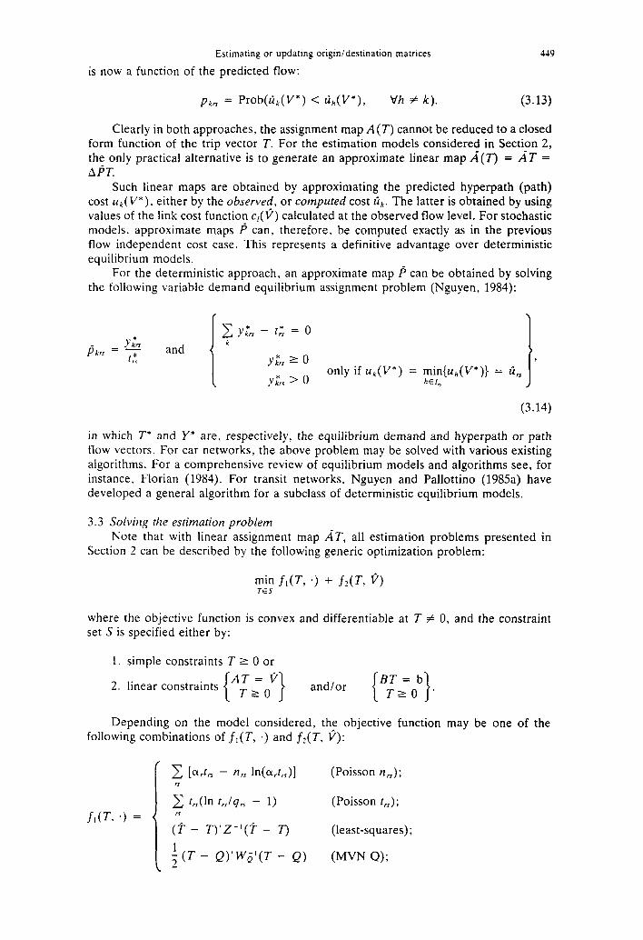
Clearly in both approaches, the assignment map A(T) cannot be reduced to a closed form function of the trip vector T. For the estimation models considered in Section 2, the only practical alternative is to generate an approximate linear map A(T) = AT = Al?

Such linear maps are obtained by approximating the predicted hyperpath (path) cost uk(V*), either by the observed, or computed cost fi k. The latter is obtained by using values of the link cost function c,(V) calculated at the observed flow level. For stochastic models. approximate maps p can, therefore, be computed exactly as in the previous flow independent cost case. This represents a definitive advantage over deterministic equilibrium models.

For the deterministic approach, an approximate map Is can be obtained by solving the following variable demand equilibrium assignment problem (Nguyen, 1984):

(3.14)

in which T* and Y* are, respectively, the equilibrium demand and hyperpath or path flow vectors. For car networks, the above problem may be solved with various existing algorithms. For a comprehensive review of equilibrium models and algorithms see, for instance, Florian (1984). For transit networks, Nguyen and Pallottino (1985a) have developed a general algorithm for a subclass of deterministic equilibrium models.

3.3 Solving the estimation problem Note that with linear assignment map AT, all estimation problems presented in

Section 2 can be described by the following generic optimization problem:

7;: f,(T, a) + f,(T, V)

where the objective function is convex and differentiable at T # 0, and the constraint set S is specified either by:

1. simple constraints T 2 0 or

2. linear constraints AT= p I and/or

BT = b TzO 1 TzO .

Depending on the model considered, the objective function may be one of the following combinations of f,(T, .) and fz( T, v):

I T [%tr* - nrs ~n(cu,)l (Poisson n,);

C Uln t,J(7,f - 1) (Poisson t,r); f,(T. .I =

;‘i. - T)‘Z-‘(i‘ - T) (least-squares);

;(T - Q)‘W;I(T - Q) (MVN Q);

450 E. CASCEITA and S. NGCYEN

c [A,T - i3/ In A,T] (Poisson);

fZ(T, P) = ;‘” 2 (ri - AT)‘W-‘(6’ - AT) (MVN).

For models that admit only a few linear constraints in addition to the nonnegativity constraints, a solution algorithm based on the projected Newton methods (see, for example Bertsekas. 1982) seems to represent a good choice. On the other hand, when deterministic traffic count constraints are imposed, then numerous algorithms for linearly constrained convex programs can be adapted for these problems (see, for example, Luenberger, 1973). However, for large-scale estimation problems with an entropy objective function:

and numerous constraints, it may be advantageous to consider a dual coordinate-wise ascent algorithm which operates on a single constraint at a time. Bregman’s efficient algorithm (Bregman, 1967) is an example of such a method.

4. A NUMERICAL EXAblPLE

To provide additional insight into the relative performance of several generic estimators, a test problem with varying input-data was generated. The 6 node 1-I link test network is shown in Fig. 1. Nodes {i,, i3, i,, i6} are centroid nodes, and a complete O/D trip demand matrix T with equal “true” average cell values t,X was assumed. Val- ues of 25 and 50 trips per unit time were successively considered.

True average link flows uI were obtained from a logit path choice model:

with 8 = 0,20 and a constant cost cl = 5 was assumed for each link 1. Observed flows ir, on links {(1,4),(4,1),(2.5),(5,2),(3,6),(6,3)} were sampled from

independent normal variates with coefficients of variation cv (standard deviation to mean ratio) of 5% and lO%, respectively. The assignment map A(T) is also displayed in Fig. 1.

The first set of simulations involved the ‘*classical” estimators-estimators that combine trip survey estimates with traffic counts. Trip “survey” counts [n,X] were obtained from a Monte Carlo simulation with sampling fraction c1 of 2 and lo%, respectively. All trips were assumed to be home-based trips for the period considered.

For each run a different set of sample trips [trI], where of, = nrr, and traffic counts [c,] was used to compute the Poisson-based ML and GLS estimates. The following models were assumed:

ML estimates

GLS estimates

(4.2)


Fig. 1. Network layout and assignment map A(T).

(1.4) 0,20 0.86 0,33 0.33 0.02 0,20 (4,l) 0,20 0.86 0.33 0.20 0.33 0.02 (2.5) 0,lO 0.12 0.33 0.10 0.33 0,12 0.10 0.10 (5.2) 0.10 0.10 0,12 0.33 0.10 0.33 0.12 0.10

0.02 0.33 0.20 0.33 0.86 0.20 0.20 0,02 0.33 0,33 0.86 0.20

in which the sampling error variance ak of the survey estimates i,5 and the flow measurement error variance af were computed, respectively, as

The mean squared errors (MSE) statistic:

MSE = 2 (bX + Var(t,J)), ,J

(4.3)

where b,5 is the theoretical bias of the estimated O/D flow rrr, was calculated for each estimator. In the present case, all estimators (T, T aML, TcLs) are unbiased. Thus, the MSE is simply the sum of their variances. The percentage reduction of the mean squared errors of the final estimates with respect to that of the initial survey estimates-a measure of the improvement produced by the addition of the traffic counts based information- was computed as follows:

A.wsdii. - TE> = MSE( 7) - MSE(T’)

MSE(?-) ’

where TE denotes either T’lL or TGLS. Results for this set of tests are reported in Tables 1 and 2.

Two conclusions can be drawn from this experiment. First, the Poisson-based ML estimator seems to be slightly better than the GLS estimator. However, this also suggests a certain robustness of the latter, since the simple random sampling scheme, used in this case, favors a maximum likelihood approach. Second, it is somewhat reassuring to see that the improvement obtained for the survey estimates, measured by the percentage reduction AMsE, is fairly consistent over the range of input data generated. The less precise the survey estimates (smaller sampling rate a), and the smaller the unknown O/D flows, the more significant is the improvement obtained. Furthermore, the more precise the traffic counts (smaller coefficient of variation cu), the larger is the improvement. The negligible negative values of AMSE in Tables 1 and 2, which arose for extreme cases-high sampling rate (a = 10%) and low traffic count precision (cu = lO%)- may be caused by computional round-off errors. Nevertheless, this suggests that in real

452 E. CASCET~A and S. NGUYEN

Table I. Performance of the Poisson-based ML estimator

(& (Z)

2 5 2 10

10 5 10 10 2 5 2 10

10 5 10 10

“True” “Survey”

[Ll MSE(?-)

25 11.125 25 11,275 25 2,290 25 2,178

150 68,712 150 66.175 150 13,031 150 12.728

Poisson-based ,ML

MSE( T”‘) A&j - ,Wi)

4,738 0.57-t 5,163 0.542 1.363 0.105 1,574 0.277

53.032 0.223 55,258 0.165 12.596 0.03-t 12.943 -0.017

a = sampling rate; CY = standard deviation to mean ratio (number of simulation runs = 200).

applications, imprecise traffic counts combined with errors in the adopted assignment model may worsen the initial survey estimates.

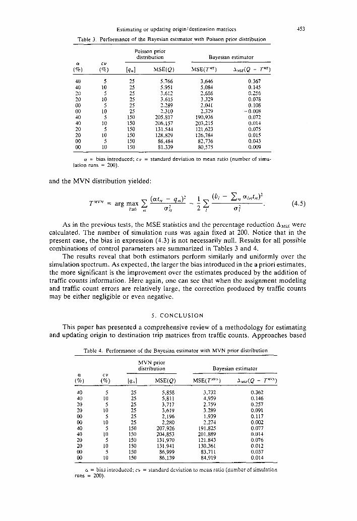
Two Bayesian estimators were examined in the second set of simulation runs. For this experiment, the “a priori” estimates Q = [qrS] were given equal cell values of 25 and 150 trips, respectively, while the “true” unknown flows T = [r,3] were generated by sampling IV, trips for each origin zone from a multinomial variate with probabilities assumed equal to the destination weights pIX = q,/q, . The number of trips IV, sampled was set equal to N, = (1 + a)qr.. A value of Q = 0 means that the a priori estimates qrr reproduce exactly the total number of trips originating from each zone, and approximately the distribution of this number among the destination zones. On the other hand, a strictly positive a implies that the a priori values underestimate the global level of mobility, even though the relative attraction to each destination zone is approximately reproduced.

Two different prior distributions were considered: a Poisson distribution with mean Q, and a MVN distribution with mean Q and a diagonal dispersion matrix WQ in which the variances a:; were calculated as follows:

With normal distributions assumed for the traffic counts, the Poisson distribution lead to the following maximum entropy estimator:

TME = arg max - TaO

Table 2. Performance of the GLS estimator

(& (;) “True”

IL1 “Survey” ME(F)

GLS

MSE(7’GL’) A,,,,@ - F’)

2 5 25 11,125 4.901 0.559

2 10 25 11,275 5,614 0.502 10 5 25 2,290 1.412 0.383 10 10 25 2,178 1.705 0.217 2 150 68,712 55,798 0.188 2 1; 150 66,175 63,086 0.047

10 5 150 13,031 12,866 0.013 In 10 150 12.728 12,786 .0.005

CI = sampling rate; CY = standard deviation to mean ratio (number of simulation runs = 200).


Table 3. Performance of the Bayesian estimator with Poisson prior distribution

453

and the MVN distribution yielded:

Poisson prior distribution Bayesian estimator

Q CY

(%b) (%)

40 5 25 5,766 3,646 0.367 40 10 25 5.951 5,084 0.145 20 5 25 3.612 2,686 0.256 20 10 25 3.615 3,329 0.078 00 5 25 2.289 2.041 0.108 00 10 25 2,310 2.329 - O.M)8 40 5 150 205.817 190.936 0.072 40 10 150 206,157 203,215 0.014 20 5 150 131.544 121,623 0.075 20 10 150 128,829 126,781 0.015 00 5 150 86,484 82,736 0.043 00 10 150 81.339 80,575 0.009

o = bias introduced; CY = standard deviation to mean ratio (number of simulation runs = 200).

(4.5)

As in the previous tests, the MSE statistics and the percentage reduction A,MSE were calculated. The number of simulation runs was again fixed at 200. Notice that in the present case, the bias in expression (4.3) is not necessarily null. Results for all possible combinations of control parameters are summarized in Tables 3 and 4.

The results reveal that both estimators perform similarly and uniformly over the simulation spectrum. As expected, the larger the bias introduced in the a priori estimates, the more significant is the improvement over the estimates produced by the addition of traffic counts information. Here again, one can see that when the assignment modeling and traffic count errors are relatively large, the correction produced by traffic counts may be either negligible or even negative.

5. CONCLUSION

This paper has presented a comprehensive review of a methodology for estimating and updating origin to destination trip matrices from traffic counts. Approaches based

Table 4. Performance of the Bayesian estimator with MVN prior distribution

MVN prior distribution Bayesian estimator

(& (& k7nl M=(Q) MSE( F”“‘) A.&Q - 7”‘v.v)

40 1; 25 5,858 3.732 0.362 40 25 5,811 4.959 0.146 20 5 25 3,717 2.759 0.257 20 10 25 3,619 3,289 0.091 00 5 25 2,196 1,939 0.117 00 10 25 2,280 2.274 0.002 40 5 150 207,926 191,825 0.077 40 10 150 204,853 201.889 0.014 20 5 150 131,970 121,843 0.076 20 10 150 131,941 130,361 0.012 00 5 150 86,999 83,711 0.037 00 10 150 86,139 84,919 0.014

Q = bias introduced; cv = standard deviation to mean ratio (number of simulation runs = 200).

45-l E. CASCETTA and S. NGUYEN

on the classical and Bayesian statistical inference techniques were examined in detail. For each approach, a generic optimization formulation of the estimation problem using an abstract traffic assignment operator was described. and computational issues dis-

cussed.

Our goal was not to promote any particular model or set of models, but rather to describe a general approach to estimating and updating origin to destination trip matrices from traffic counts. This approach is intended to serve as a framework within which problem-specific models can be crafted and solution algorithms developed.

REFERENCES

Bell G. H. A. (1983) The estimation of an origin-destination matrix from traffic counts, Trenspn. Sci. 10. 198-217.

Ben-Akiva M. E., Macke P. P. and Hsu P. S. (1985) Alternative methods to estimate route-level trip tables and expand on-board surveys. TRB, Transpn. Res. Rec. 1037. l-1 1.

Bertsekas D. P. (1982) Projected Newton methods for optimization problems with simple constraints. S/AM J. Control Optim. 20, 221-216.

Bevy P. H. L. and Jensen G. R. M. (1983) Network aggregation effects upon equilibrium assignment outcomes: An empirical investigation. Transpn. Sci. 17, 240-262.

Bregman L. M. (1967) The relaxation method of finding the common point of convex sets and its application to the solution of problems in convex programming. USSR Computational Mafhemafics and Mathemafical Physics 7, 200-217.

Cascetta E. (1984) Estimation of trip matrices from traffic counts and survey data: A generalized least squares estimator. Transpn. Res. 18B. 289-299.

Cascetta E. (1986) A Class of Travel Demand Esfimafors Using Traffic Flotvs. Publication 375. Centre de Recherche sur les Transports. Universite de Montreal.

Cascetta E. and Nuzzolo A. (1986a) Empirical analysis of urban network assignment models. Proceedings of rhe 4’h Nationa Congress of the Progetto Finali zzafo Trasporfi. Torino. October 1986.

Cascetta E. and Nuzzolo A. (1986b) A behavioral model of path choice in urban transit networks. Proceedings of the ja Nafional Congress of fhe Progeffo Finalizzato Trasporti. Torino. October 1986.

Chriqui C. and Robillard P. (1975) Common bus line. Transpn. Sci. 9. 115-121. Daganzo C. F. (1979) Multinomial Probit: The Theory and Its Application to Demand Forecasting. Academic

Press. New York. Daganzo C. F., Bouthelier F. and Sheffi Y. (1977) Multinomial probit and qualitative choice: A computationally

efficient algorithm. Trunspn. Sci.11, 338-358. Daganzo C. F. and Sheffi Y. (1977) On stochastic models of traffic assignment. Transpn. Sci. 11, 253-274. Dial R. B. (1971) A probabilistic multipath traffic assignment model which obviates path enumeration. Transpn.

Res. 5, 83-111. Dial R. B., Glover F., Karney D. and Klingman D. (1979) A computational analysis of alternative algorithms

and labeling techniques for finding minimum cost alternative trees. iVefworks 9, 215-248. Domencich T. A. and McFadden D. (1975) Urban Travel Demand: A Behavioral Analysis. American Elsevier.

New York. Florian M. and Fox B. (1976) On the probabilistic origin of Dial’s multipath traffic assignment model. Trtmspn.

Res. 10. 339-341. Florian M. and Nguyen S. (1976) An application and validation of equilibrium trip assignment methods.

Transpn. Sci. 10, 374-389. Florian M. (1984) An introduction to networks models used in transportation planning. In Transportation

PIanning Mode/s (M. Florian. ed.), pp. 137-152. Elsevier Science Publishers B. V. (North Holland). Amsterdam.

Gallo G.. Pallottino S.. Ruggeri S. and Storchi G. (1982) Bib1iograph.v on minimum cosf alternarives. Rapport0 technico, C. N. R.. Progetto Finalizzato Informatica. SOFIMAT.

Gallo G. and Pallottino S. (1984) Minimum cost alternative methods in transportation models. In Trunsportafion Planning Models (M. Florian. ed.). pp. 227-256. Elsevier Science Publishers B. V. (North Holland). Amsterdam.

Inaudi D. and Morello E. (1985) Aspetti applicativi di un modello di equilibrio per reti di trasporto public0 urbane. Proceedings of fhe 3’d National Congress of the Progetto Finalizzato Trasporti, Taormina, May 1985.

Judge G. G., Griffiths W. E.. Hill R. C. and Lee T. C. (1980) The Theory and Pracfice of Econometrics. Wiley, New York.

Kullback S. (1959) Information Theory and Sfutistic. Wiley, New York. Landau U.. Hauer E. and Geva I. (1982) Estimation of cross-cordon origin-destination flows from cordon

studies. TRB. Transpn. Res. Rec. 891, 5-10. Langdon M. G. (1984) Methods of determining choice probability in utility maximizing multiple alternative

models. Transpn. Res. 18B, 209-233. Luenberger D. G. (1973) Inrroduction to Linenr and Nonlinear Programming. Addison Wesley. Reading.

Mass. Maher M. J. (1983) Inferences on trip matrices from observations on link volumes: a Bayesian statistical

approach. Transpn. Res. 17B. 435447. Manski C. F. and McFadden D. L. (1981) Alternative estimators and sample design for discrete choice analysis.

In Sfructural Analysis of Discrete Data with Econometric Application (C. Manski and D. McFadden. eds.). MIT Press, Cambridge, Massachusetts.

Estimating or updating origin/destination matrices 4%

McNeil S. (1983) Quadratic matrix entry estimation methods. Ph.D. thesis, Dept. of Civil Engineering, Carnegie-Mellon University, Pittsburgh, Pennsylvania.

Nguyen S. (1983) Modele de distribution spatiale tenant compte des itintraires. INFOR 21(4), 270-292. Nguyen S. (1984) Estimating origin-destination matrices from observed flows. In Transporturion Planning

Models (M. Florian, ed.), pp. 363-380. Elsevier Science Publishers B. V. (North Holland), Amsterdam. Nguyen S. and Pallottino S. (1985a) Equilibrium Traffic Assignmenf for Large Scale Transit Networks. Quar-

derno 14, IAC, C. N. R., Roma. Nguyen S. and Pallottino S. (1985b) Assegnamento dei Passeggeri ad un Sistema di Linee Urbane: Deter-

minazione degli Ipercamini Minimi. Ricerca Operativa 38, 29-78. Snickars F. and Weibull J. W. (1977) A minimum information principle, theory and practice. Region. Sci.

Urban Econ. 7, 137-168. Sobel K. L. (1980) Travel demand forecasting with the nested multinomial logit model. Proceedings of the

59” Annual Meeting of the Transportation Research Board, Washington D.C.. January 1980. Spiess H. (1983a) A Maximum Likelihood Model for Estimating Origin-Destination Matrices. Publication 293,

Centre de Recherche sur les Transports, Universite de Montreal. Spiess H. (1983b) On Optimal Choice Strategies in Transit Networks. Publication 286, Centre de Recherche

sur les Transports, UniversitC de Montrtal. Taylor M. A. P. (1979) Evaluating the performance of a simulation model. Transpn. Res. 13A, 1.59-173. Van Zuylen J. H. and Branston D. M. (1982) Consistent link flows estimation from counts. Trunspn. Res.

16B, 473-476. Van Zuylen J. H. and Willumsen L. G. (1980) The most likely trip matrix estimated from traffic counts.

Transpn. Res. 14B, 281-293. Wardrop J. G. (1952) Some theoretical aspects of road traffic research. Proc. Inst. Civil Engr., Part If 1, 325-

378. Williams H. C. W. L. (1977) On the formation of travel demand models and economic evaluation measures

of user benefit. Environ. Plan. A 9, 285-344. Wilson A. G. (1970) Entropy in Urban and Regional Modeling. Methuen, Inc., New York. Yates F. (1981) Sampling Methods for Censures and Surveys. Griffin, London.

A unified framework for estimating or updating origin/destination matrices from traffic counts

Documents

Transcript of A unified framework for estimating or updating origin/destination matrices from traffic counts