Meta-analytic Structural Equation Modeling with Covariance Matrices 1

Running head: Meta-analytic Structural Equation Modeling with Covariance Matrices

A Two-Stage Approach to Synthesizing Covariance Matrices

in Meta-Analytic Structural Equation Modeling

Mike W.-L. Cheung

National University of Singapore

Wai Chan

Chinese University of Hong Kong

This is a post-print version of the following paper:

Cheung, M. W.-L., & Chan, W. (2009). A two-stage approach to synthesizing covariance

matrices in meta-analytic structural equation modeling. Structural Equation Modeling: A

Multidisciplinary Journal, 16(1), 28–53. http://doi.org/10.1080/10705510802561295

Meta-analytic Structural Equation Modeling with Covariance Matrices 2

Abstract

Structural equation modeling (SEM) is widely used as a statistical framework to test complex

models in behavioral and social sciences. When the number of publications increases, there is a

need to systematically synthesize them. Methodology of synthesizing findings in the context of

SEM is known as meta-analytic structural equation modeling (MASEM). Although correlation

matrices are usually preferred in MASEM, there are cases that synthesizing covariance matrices

is useful, especially when the scales of the measurement are comparable. This study extends the

two-stage structural equation modeling (TSSEM) approach proposed by M. W. L. Cheung and

Chan (2005a) to synthesizing covariance matrices in MASEM. A simulation study was

conducted to compare the TSSEM approach with several approximate methods. An empirical

example was used to illustrate the procedures. Future directions for MASEM were discussed.

Keywords: meta-analytic structural equation modeling, meta-analysis, Fisher’s z transformation

Meta-analytic Structural Equation Modeling with Covariance Matrices 3

A Two-Stage Approach to Synthesizing Covariance Matrices

in Meta-Analytic Structural Equation Modeling

Structural equation modeling (SEM) is widely used as a statistical framework to test

models involving observed and latent variables in behavioral and social sciences (e.g.,

Hershberger, 2003; Tremblay & Garden, 1996). However, it is often found that researchers are

reluctant to consider alternative models (MacCallum & Austin, 2000). This confirmation bias, a

prejudice in favor of the model being evaluated, hinders the development of research progress

(Greenwald et al., 1986). Consistent conclusions may not be easily reached even there are many

empirical studies on the same topic. This prompts the need of systematically comparing and

integrating research findings in the context of SEM.

Meta-analysis, a term coined by Glass (1976), is usually employed as a statistical

approach to synthesize research findings in medical, behavioral and social sciences (e.g., Hedges

& Olkin, 1985; Hunter & Schmidt, 2004; National Research Council, 1992). Two common

objectives of meta-analysis are to test the homogeneity of findings and to synthesize the findings.

It is intuitive to combine meta-analytic techniques and SEM in testing complex models from a

pool of studies (e.g., B. J. Becker & Schram, 1994; M. W. L. Cheung, 2002; M. W. L. Cheung &

Chan, 2005a; S. F. Cheung, 2000; Furlow & Beretvas, 2005; Hafdahl, 2001; Hunter & Schmidt,

2004; Shadish, 1996; Viswesvaran & Ones, 1995).

Several terms have been used interchangeably in the literature, for instance, meta-analytic

path analysis (Colquitt, LePine, & Noe, 2000), meta-analysis of factor analysis (G. Becker,

1996), meta-analytical structural equations analysis (Hom, Caranikas-Walker, Prussia, &

Griffeth, 1992), path analysis of meta-analytically derived correlation matrices (Eby, Freeman,

Rush, & Lance, 1999), structural equation modeling of a meta-analytic correlation matrix

Meta-analytic Structural Equation Modeling with Covariance Matrices 4

(Conway, 1999) and path analysis based on meta-analytic findings (Tett & Meyer, 1993). In this

paper we use the generic term meta-analytic structural equation modeling (MASEM) to describe

this class of techniques (see M. W. L. Cheung & Chan, 2005a).

Correlation matrices are usually used in MASEM because the measurement or scales of

the variables are likely different across studies (Hunter & Hamilton, 2002; Hunter & Schmidt,

2004). However, covariance matrices preserving the scales of the variables may sometimes be

preferred when the same measurement is used in all studies and the scales of the variables are of

interest. For example, it is of interest to test whether the scales (variances) of the measurement

are the same in cross-cultural research where the same measurement is usually used (M. W. L.

Cheung, Leung, & Au, 2006). Recently, Beretvas and Furlow (2006) proposed an approximate

method to synthesize covariance matrices in MASEM. Specifically, they suggested synthesizing

correlation matrices and standard deviations separately. The pooled correlation matrix and the

pooled standard deviations are combined to obtain a pooled covariance matrix. The pooled

covariance matrix is then used to fit structural models.

M. W. L. Cheung and Chan (2005a) proposed a two-stage structural equation modeling

(TSSEM) approach to conduct MASEM with correlation matrices. Although they mentioned that

their approach could be extended to covariance matrices (M. W. L. Cheung & Chan, 2005a),

they did not provide any details and computational procedures. The main objective of the present

study is to extend the TSSEM approach to synthesizing covariance matrices in the context of

MASEM. In the following sections, we first summarize approaches on MASEM with correlation

and covariance matrices. Next, we present the TSSEM approach and its advantages in

synthesizing covariance matrices. The proposed approach is empirically evaluated against the

approximate methods proposed by Beretvas and Furlow (2006) via computer simulation. An

Meta-analytic Structural Equation Modeling with Covariance Matrices 5

empirical example is used to illustrate the procedures. Finally, we discuss the future research

directions in MASEM.

Meta-analytic Structural Equation Modeling

Synthesizing Correlation Matrices

Meta-analytic structural equation modeling is usually conducted via two stages

(Viswesvaran & Ones, 1995). In the first stage, meta-analytic techniques are applied on a series

of correlation matrices to create a pooled correlation matrix. Univariate and multivariate methods

may be used to pool the correlation matrices. If the correlation matrices are homogeneous, a

pooled correlation matrix is estimated. In the second stage, the pooled correlation matrix is used

as the observed covariance matrix to fit structural models, which can be path models,

confirmatory factor analytic (CFA) models, or general structural models.

Stage 1: Estimating a pooled correlation matrix. In the present study, we denote )( gT as

a generic effect size in the gth study. The effect size )( gT can be expressed as

)()()( ggg eT , (1)

where )( g and )( ge are the population effect size and the sampling error in the gth study,

respectively. )( ge is assumed normally distributed with a mean of zero and a sampling variance

of 2)( )( g . It can be shown (e.g., Hedges & Olkin, 1985) that the weighted average T is

K

g

g

K

g

gg

w

Tw

T

1

)(

1

)()(

, (2)

where 2)()( )/(1 ggw is the weight and K is the total number of studies. The sampling variance

2

Ts of T is estimated by

Meta-analytic Structural Equation Modeling with Covariance Matrices 6

K

g

g

Tws

1

)(2 /1 . (3)

When univariate methods are used, each correlation coefficient is combined individually

with Pearson correlations (univariate r method; Hunter & Schmidt, 2004) or Fisher’s z scores

(univariate z method; Hedges & Olkin, 1985). The univariate r method computes the average of

individual correlation coefficients by weighted by their sampling variance,

K

g

gr

K

g

ijg

r

ij

w

rw

r

(g)

1

)(

1

)(

(4)

where ijr is the pooled correlation coefficient for the ith and jth variables,

22)()()( ))(1/( gij

ggr rnw , )( g

ijr and )(gn are the sample correlation and sample size in gth study,

respectively.1

The sampling distribution of the correlation coefficient becomes skewed when the

population correlation deviates from zero. Hedges and Olkin (1985) argued using Fisher’s z

transformed scores on averaging correlation coefficients. The sample correlation )( gijr is first

transformed to a Fisher’s z score )(gijz by

)1

1(log

2

1(g)

(g)

(g)

ij

ijij

r

rz

(5)

where log(.) is the natural logarithm. Then the pooled Fisher’s z score, ijz , for ith and jth

variables can be obtained by

K

g

gz

K

g

ijg

z

ij

w

zw

z

(g)

1

)(

1

)(

, (6)

Meta-analytic Structural Equation Modeling with Covariance Matrices 7

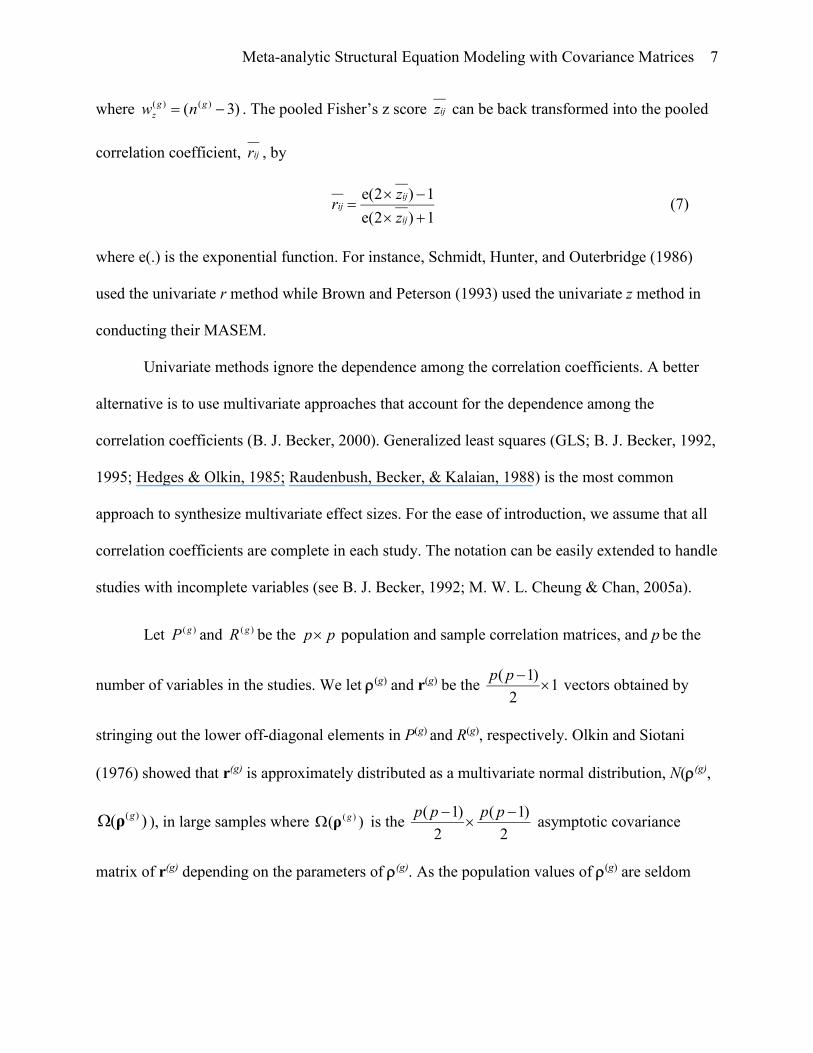
where )3( )()( ggz nw . The pooled Fisher’s z score ijz can be back transformed into the pooled

correlation coefficient, ijr , by

1)2e(

1)2e(

ij

ijij

z

zr (7)

where e(.) is the exponential function. For instance, Schmidt, Hunter, and Outerbridge (1986)

used the univariate r method while Brown and Peterson (1993) used the univariate z method in

conducting their MASEM.

Univariate methods ignore the dependence among the correlation coefficients. A better

alternative is to use multivariate approaches that account for the dependence among the

correlation coefficients (B. J. Becker, 2000). Generalized least squares (GLS; B. J. Becker, 1992,

1995; Hedges & Olkin, 1985; Raudenbush, Becker, & Kalaian, 1988) is the most common

approach to synthesize multivariate effect sizes. For the ease of introduction, we assume that all

correlation coefficients are complete in each study. The notation can be easily extended to handle

studies with incomplete variables (see B. J. Becker, 1992; M. W. L. Cheung & Chan, 2005a).

Let )( gP and )( gR be the pp population and sample correlation matrices, and p be the

number of variables in the studies. We let (g) and r(g) be the 12

)1(

pp vectors obtained by

stringing out the lower off-diagonal elements in P(g) and R(g), respectively. Olkin and Siotani

(1976) showed that r(g) is approximately distributed as a multivariate normal distribution, N((g),

)( )(gρ ), in large samples where )( )( gρ is the 2

)1(

2

)1(

pppp asymptotic covariance

matrix of r(g) depending on the parameters of (g). As the population values of (g) are seldom

Meta-analytic Structural Equation Modeling with Covariance Matrices 8

known, their sample estimates r(g) are often substituted in )( )( gρ , i.e., )( )(gr . The elements of

variances and covariances of )( )( gρ are then calculated by,

)(

22)1(

) var(g

ij

ijn

rr

, (8)

)(5.0[),cov(2222

jljkiliklkijklij rrrrrr )(/)]( glkljlilkkjkijljkjiilikijjkiljlik nrrrrrrrrrrrrrrrr .

To simplify the presentation, the superscript (g) in the correlation coefficients is skipped from

the above equation.

Let ρ be a 12

)1(

pp vector that contains the population correlations. Then for the gth

study, we define a 2

)1(

2

)1(

pppp selection matrix, )( gG , with 0’s and 1’s that select the

appropriate correlation coefficients in the gth study. Since it is assumed that there is no

incomplete variable, )( gG is simply an identity matrix.

We then let TT)()2()1( |...|| KGGGG TT be a matrix obtained by stacking the selection

matrices from the K studies, where (.)T is the transpose of the matrix. By assuming a linear

combination of true correlation vector and sampling error, the observed correlation vector can be

expressed as

eρr G (9)

where TT)(T)2(T)1( |...|| Krrrr and e is a 1)2

)1((

1

g

k

ppvector of random errors with E(e) = 0,

it can be shown that the value of estimated via GLS is

rρ 1T-11T Ω)Ω(ˆ GGG (10)

Meta-analytic Structural Equation Modeling with Covariance Matrices 9

where )()2()1( ,...,,Diag k , Diag() is a diagonal matrix, and )( )()( kk r (B. J. Becker,

1992; Hedges & Olkin, 1985).

The GLS approach can also be extended to Fisher’s z scores. The asymptotic covariance

matrix of the Fisher’s z scores is first estimated (see Steiger, 1980 for the formula). Then

Equation 10 is applied to obtain a pooled matrix of Fisher’s z scores (B. J. Becker & Fahrbach,

1994).

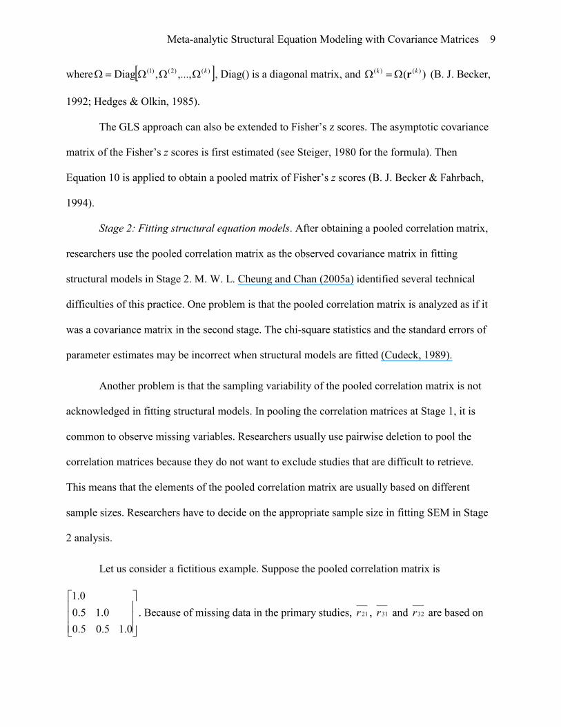
Stage 2: Fitting structural equation models. After obtaining a pooled correlation matrix,

researchers use the pooled correlation matrix as the observed covariance matrix in fitting

structural models in Stage 2. M. W. L. Cheung and Chan (2005a) identified several technical

difficulties of this practice. One problem is that the pooled correlation matrix is analyzed as if it

was a covariance matrix in the second stage. The chi-square statistics and the standard errors of

parameter estimates may be incorrect when structural models are fitted (Cudeck, 1989).

Another problem is that the sampling variability of the pooled correlation matrix is not

acknowledged in fitting structural models. In pooling the correlation matrices at Stage 1, it is

common to observe missing variables. Researchers usually use pairwise deletion to pool the

correlation matrices because they do not want to exclude studies that are difficult to retrieve.

This means that the elements of the pooled correlation matrix are usually based on different

sample sizes. Researchers have to decide on the appropriate sample size in fitting SEM in Stage

2 analysis.

Let us consider a fictitious example. Suppose the pooled correlation matrix is

0.15.05.0

0.15.0

0.1

. Because of missing data in the primary studies, 21r , 31r and 32r are based on

Meta-analytic Structural Equation Modeling with Covariance Matrices 10

sample sizes of 1,000, 500 and 200, respectively. However, the sample sizes for these correlation

coefficients are assumed equal in fitting SEM in Stage 2. If 1,000 is used as the sample size, the

sample sizes for 31r and 32r are overestimated. In other words, the standard errors of 31r and 32r

will be under-estimated. If 500 is used as the sample size in the analysis, the standard errors of

21r and 32r are over-estimated and under-estimated, respectively.

Different ways for determining the sample size have been used in the literature, for

example, the arithmetic mean (Carson, Carson, & Roe, 1993; Premack & Hunter, 1988;

Verhaeghen & Salthouse, 1997), the harmonic mean (Colquitt, LePine, & Noe, 2000; Conway,

1999), the median (Brown & Peterson, 1993) or the total (Hunter, 1983; Tett & Meyer 1993) of

the sample sizes based on the synthesized correlation coefficients. It should be noted that all of

these suggested methods are ad-hoc and without strong statistical support. Because the Type I

error of the chi-square test statistics, goodness-of-fit indices, statistical power, and standard

errors of parameter estimates are all related to the sample size used (Bollen, 1989), using

different sample sizes may result in different inferences.

M. W. L. Cheung and Chan (2005a) conducted several simulation studies to evaluate the

performance of these conventional approaches. They found that the univariate approaches work

well in testing the homogeneity of correlation matrices in Stage 1 while they are too liberal in

controlling the Type I error in Stage 2. On the other hand, the GLS approach performs poorly

unless the average sample size per study is very large (n>1,000 per study).

It is speculated that the poor performance of the GLS approach is due to the use of the

study-specific covariance matrices estimated in Equation 8. If the estimated asymptotic

covariance matrix of the correlation coefficients is not stable, results based on the GLS approach

will become inaccurate. Several suggestions have been made to improve the GLS performance.

Meta-analytic Structural Equation Modeling with Covariance Matrices 11

These include using Fisher’s z score with the GLS approach (B. J. Becker, & Fahrbach, 1994)

and using average correlations instead of study-specific correlations in Equation 8 (e.g., B. J.

Becker & Fahrbach, 1994; S. F. Cheung, 2000; Furlow &, Beretvas, 2005).

Synthesizing Covariance Matrices

Beretvas and Furlow (2006) argued that covariance matrices are preferred in fitting scale

non-invariant models. To pool covariance matrices, they suggested synthesizing the correlation

matrices and the standard deviations separately. Since the sample standard deviations are not

normally distributed, Beretvas and Furlow (2006) suggested transforming them to

)1(2

1)log(

)(

)()(

g

gu

gu

nsd , (11)

where )( gus and )(gn are the sample standard deviation for the ith variable, and the sample size in

the gth study, respectively. After the transformation, the sampling variance of )( gud can be

approximated by )1(2

1)( gn

(Raudenbush & Bryk, 2002). Then the transformed standard

deviations can be pooled together by Equation 2.

When a multivariate approach is used to synthesize the standard deviations, the estimated

covariance between the transformed standard deviations )( gud and )( g

vd is approximated by

)1(2 )(

2)(,

g

uvgdvdu

n

r , (12)

where uvr is the correlation between variables u and v. GLS approach can be used to synthesize

standard deviations. Once the pooled correlation matrix and the pooled standard deviations are

Meta-analytic Structural Equation Modeling with Covariance Matrices 12

available, it is easy to calculate the pooled covariance matrix. Then the pooled covariance matrix

with the total sample size as the sample size is used to fit structural models in the second stage.

A TSSEM Approach to Synthesizing Covariance Matrices

Pooled correlation matrix is usually used as a covariance matrix in conventional MASEM.

In the SEM community, it is well-known that fitting correlation matrices as covariance matrices

may result in incorrect test statistics and standard errors (Cudeck, 1989). M. W. L. Cheung and

Chan (2005a) proposed a TSSEM approach to conduct MASEM on correlation matrices.

Specifically, they proposed using a multiple-group CFA model to test the homogeneity of the

correlation matrices and to synthesize the matrices in Stage 1.

In the second stage, the pooled correlation matrix is then used to fit structural models

with the asymptotic covariance matrix of the pooled correlation matrix as the weight matrix by

the weighted least squares (WLS) method, which is equivalent to Browne’s (1984)

asymptotically distribution-free method. The Stage-1 and Stage-2 analyses are known as “Case

C” and “Case D” analyses of correlation matrices in Jöreskog, Sörbom, Du Toit, and Du Toit

(1999). Browne and Arminger (1995), and Fouladi (2000) also provided detailed discussion on

how to fit correlation structures and correlation matrices in SEM.

Stage 1: Testing Homogeneity of Covariance Matrices and Estimating Pooled Covariance

Matrix

It is well-known that a covariance matrix can be decomposed into the matrices of

standard deviations and correlations by

T)()()()()( gggg θ (13)

Meta-analytic Structural Equation Modeling with Covariance Matrices 13

where )( g is a )()( gg pp diagonal matrix of factor loadings and )(g is a )()( gg pp

standardized matrix of factor correlations (e.g., Bentler, 1995; Bentler & Lee, 1983; Jöreskog &

Sörbom, 1996; Jöreskog et al., 1999; Krane & McDonald, 1978). The standardized factor

correlation matrix )(g and the diagonal factor loading matrix )( g represent the sample

correlation matrix and the standard deviations, respectively (also see M. W. L. Cheung, in press;

M. W. L. Cheung & Chan, 2004 and Raykov, 2001 for other applications of similar

parameterizations). Since the dimensions of the covariance matrices can be different across

studies, incomplete variables can be handled easily.

To pool correlation matrices, we can impose equality constraints on (g) across studies.

The estimate under these constraints is the estimate of the pooled correlation matrix. As the

constrained model and the unconstrained model are nested, we may use chi-square difference test

to test the homogeneity of the correlation matrices. Moreover, goodness-of-fit indices may also

be used to assess the adequacy of the homogeneity of correlation matrices.

The above approach can be easily modified to pool covariance matrices. We can use:

T)()()()()( gggg II θ (14)

where )( g is the )()( gg pp covariance matrix and )( gI is a )()( gg pp identity matrix in the

gth study. We can then pool the covariance matrices together by imposing the following

constraint:

)()2()1( K . (15)

The estimate under these constraints is the estimate of the pooled covariance matrix. This

approach has been frequently applied to test the homogeneity of covariance matrices in the SEM

literature (e.g., Jöreskog & Sörbom, 1996; Raykov, 2001). Chi-square difference test and other

goodness-of-fit indices may be used to assess the homogeneity of the covariance matrices.

Meta-analytic Structural Equation Modeling with Covariance Matrices 14

An equivalent parameterization of the above model is to impose equality constraints on

the standard deviations and correlations separately. That is, we set )()2()1( K and

)()2()1( K simultaneously in Equation 13. The chi-square statistic and other

goodness-of-fit indices are the same as those under Equations 14 and 15. However, estimates of

the pooled covariance matrix are decomposed into estimates of the pooled correlation matrix and

the pooled standard deviations. This decomposition is not suitable for the Stage 2 analysis in

which the covariance matrix and its asymptotic covariance matrix are expected. Nevertheless,

this parameterization is very useful in testing the homogeneity of variances (see the empirical

example).

Stage 2: Fitting Structural Models

After the analysis from Stage 1, we have estimates of a pooled pp covariance matrix

S with its 2

)1(

2

)1(

pppp asymptotic covariance matrix of parameter estimates V and the

total sample size N which equals the sum of all sample sizes, i.e.,

K

g

gnN1

)( .

Similar to the approach proposed by M. W. L. Cheung and Chan (2005a), we use S as

the observed covariance matrix and its asymptotic covariance matrix V as the weight matrix

with the WLS as the estimation method. The fit function for the structural model is

))(*(ˆ))(*()( 1T θθθ sVsF (16)

where *s and )(θ are the 1*p vectors of 1)/2(* ppp elements obtained by stringing out

the lower triangular elements in S and in the implied covariance matrix )(θ , respectively. V is

a ** pp weight matrix estimated from the first stage and is a structural parameter vector of

the proposed model (Jöreskog, et al., 1999).

Meta-analytic Structural Equation Modeling with Covariance Matrices 15

We mentioned in a previous section that conventional approaches in MASEM do not take

into consideration of the precision of the estimates from Stage 1. In other words, it is difficult to

choose an appropriate sample size in the Stage 2 analysis because the elements of the pooled

correlation matrix are based on different sample sizes. Recall our example with a pooled

correlation matrix of

0.15.05.0

0.15.0

0.1

, in which 21r , 31r and 32r are based on sample sizes of

1,000, 500 and 200, respectively. In the TSSEM approach a 33 asymptotic covariance matrix

of the pooled correlation coefficients will be used as the weight matrix in the analysis. Since 21r ,

31r and 32r are based on different sample sizes, the elements of the asymptotic covariance matrix

would be different. For example, the asymptotic variance on 21r will be smaller than those on

31r and 32r because 21r is based on a larger sample size (thus a smaller standard error). Since V

is inverted in Equation 16, more weight will be given to 21r than to 31r and 32r . Therefore, the

TSSEM approach takes the precision of the estimates from Stage 1 into account by using

different weights in Equation 16. This is also consistent with the general principle in meta-

analysis- more weight is given to estimates with higher precision (smaller standard error;

Equation 2).

The fitting procedure can be implemented with SEM packages such as LISREL (Jöreskog

& Sörbom, 1996) and Mx (Neale, Boker, Xie, & Maes, 2006). It should be noted that both

LISREL and Mx expect that the asymptotic covariance matrix estimated from Stage 1 is

multiplied by the sample size before being used as the weight matrix in the Stage 2 analysis

(Jöreskog et al., 1999, p. 193; Neale et al., 2006, p.41).2

Meta-analytic Structural Equation Modeling with Covariance Matrices 16

There are several advantages of using the TSSEM approach to synthesize covariance

matrices. First, the model is well integrated into SEM. Both pooling covariance matrices (Step 1

analysis) and fitting structural models (Step 2 analysis) are conducted with some existing SEM

packages, e.g., LISREL. This enables researchers with basic knowledge in SEM to conduct

MASEM with correlation or covariance matrices. Second, many techniques in SEM can be

directly applied to MASEM. For example, the TSSEM approach, that is a special case of the

general SEM, is efficient in handling incomplete variables (e.g., Allison, 1987; Muthén, Kaplan,

& Hollis, 1987) that are common in MASEM.

Third, the TSSEM approach can be easily used to test the homogeneity of variances. If it

is found that the homogeneity of covariance matrices is not tenable, researchers may want to

know whether this is due to the heterogeneity of correlation matrices or the heterogeneity of

variances or both. Since SEM approach is used, it is easy to constrain the equality on (g) but not

on (g) across studies in Equation 13 (see the illustration on an empirical example below). The

homogeneity of covariance matrices is nested within both the homogeneity of correlation

matrices and the homogeneity of variances. Chi-square difference test may be used to compare

these models. Researchers may have a better idea on whether the structures (correlation matrices)

or the scales (variances) are different. If the heterogeneity of covariance matrices is due to the

heterogeneity of variances, researchers may choose to synthesize correlation matrices as outlined

in M. W. L. Cheung and Chan (2005a).

A Simulation Study

In this section, a simulation study was conducted to investigate the performance of the

TSSEM approach and the approximate methods proposed by Beretvas and Furlow (2006) in

synthesizing covariance matrices and fitting CFA models. A two-factor CFA model with three

Meta-analytic Structural Equation Modeling with Covariance Matrices 17

indicators per factor was used in the study. This model was the same as the one used in M. W. L.

Cheung and Chan (2005a). The factor loadings for the variables were 0.8, 0.7, and 0.6 for each

factor while the factor correlation was .30. The error variances were fixed correspondingly at

0.36, 0.51, and 0.64. As covariance matrices were used in this study, the above correlation

structure was rescaled by the population standard deviations of the observed variables.

Method

Data generation. R (R Development Core Team, 2007) was used to generate multivariate

normal data with known covariance structures. The raw data were converted into covariance

matrices simulating the cases for MASEM with covariance matrices. Procedures implementing

the approximate methods were programmed in R. LISREL 8.80 (Jöreskog & Sörbom, 2006) and

a DOS program performing data manipulation (M. W. L. Cheung, 2007a) were used to conduct

the TSSEM approach. For the ease of manipulation, all variables are assumed complete. This

assumption can be justified in cross-cultural research in which there are usually no missing

variables (e.g., M. W. L. Cheung, Leung, & Au, 2006). One thousand replications were used in

each condition.

Number of studies (NS). Three levels of NS were considered: 10, 20 and 30. These are

similar to the settings used in previous simulation studies for MASEM (e.g., M. W. L. Cheung &

Chan, 2005a; 2005b; Beretvas & Furlow, 2006).

Population standard deviations (PS). Two levels of PS were considered: 1.0 and 3.0. In

the condition of PS=1.0, the population values were the same as the one in the correlation

structure. In the condition of PS=3.0, the population values were

0.13.0

0.1,

T

8.11.24.2000

0008.11.24.2, and 76.559.424.376.559.43.24Diag .

Meta-analytic Structural Equation Modeling with Covariance Matrices 18

Average sample sizes per study (AS). In applied settings, the sample sizes of studies may

be unequal. In this study the sample size per study was assumed normally distributed with a

mean of average sample size and standard deviation of one-fourth of the mean (M. W. L. Cheung

& Chan, 2005b; Field, 2001). Three levels of AS were considered: 100, 300 and 1,000. Thus, the

standard deviations of the sample sizes were 25, 75 and 250. Since the sample sizes were

randomly generated, it is possible that the resultant sample sizes were negative. To safeguard this

problem, the sample size of 20 was used as the minimum sample size per study.

Methods of Synthesizing Covariance Matrices. The first method was the TSSEM

approach proposed in this study. Beretvas and Furlow (2006) proposed several univariate and

multivariate methods in synthesizing covariance matrices with correlation coefficient and

Fisher’s z score. Four such methods were considered in this simulation study. The first two

approximate methods were the univariate methods in synthesizing correlation coefficients

(Equation 4) and Fisher’s z scores (Equation 6). The transformed standard deviations with

Equation 11 were pooled individually. The pooled correlation matrices and the pooled standard

deviations were then back transformed into a pooled covariance matrix. They were denoted as

the univariate approach to synthesizing correlations and standard deviations (uni.r.sd) and the

univariate approach to synthesizing Fisher’s z scores and standard deviations (uni.z.sd) here.

The other two approximate methods were the multivariate approaches in synthesizing

correlation coefficients and Fisher’s z scores. As indicated in previous studies (e.g., B. J. Becker

& Fahrbach, 1994; M. W. L. Cheung & Chan, 2005a; S. F. Cheung, 2000; Furlow &, Beretvas,

2005), the conventional GLS approach does not work well. Hence, the univariate pooled

correlations and Fisher’s z scores were used to calculate the asymptotic covariance matrix of the

correlation coefficients (Equation 8) and Fisher’s z scores (based on Steiger’s 1980 formula).

Meta-analytic Structural Equation Modeling with Covariance Matrices 19

The univariate pooled correlations and the pooled Fisher’s z scores back converted into

correlations were also used to calculate the asymptotic covariance matrix of the transformed

standard deviations in Equation 12. These two methods were denoted as the multivariate

approach to synthesizing correlations and standard deviations (mul.r.sd) and the multivariate

approach to synthesizing Fisher’s z scores and standard deviations (mul.z.sd) here.

All these four approximate methods are based on the GLS approach. The univariate

methods assume the effect sizes are uncorrelated while the multivariate methods take the

correlation among the effect sizes into consideration. Therefore, chi-square statistics on testing

the homogeneity of effect sizes (correlations and standard deviations) could be calculated in

Stage 1. Maximum likelihood was used as the estimation method with the total sample size as

the sample size in fitting the CFA model in Stage 2.

Assessment of the Empirical Performance. Several criteria were used to evaluate the

empirical performance of these methods. The first one was the empirical rejection rates of the

chi-squared tests computed in the two stages. Specifically, the hypothesis of the homogeneity of

covariance matrices was tested in Stage 1, and the proposed two-factor model was tested in Stage

2. As the syntheses of correlation matrices and standard deviations are considered as independent

in the approximate methods, the sum of these two chi-square statistics is assumed distributed as a

chi-square variate with the appropriate degrees of freedom. Since the data were generated from

known structures with correctly specified models, the chi-square test statistics at both Stages

were expected to follow chi-square distributions with the corresponding degrees of freedom. If

the methods are good, the rejection percentage should be close to its theoretical value (.05 in this

study).

Meta-analytic Structural Equation Modeling with Covariance Matrices 20

The second measure was the relative percentage bias of each parameter estimate, which is

defined as

%100ˆ

)ˆ(

B , (17)

where is the population value of the parameter and is the mean of the estimates of the

parameters across all replications. Good estimation methods should have relative percentage bias

less than 5% (Hoogland & Boomsma, 1998). The final measure was the relative percentage bias

of the standard error of each parameter estimate, which is defined as

%100)ˆ(

)ˆ()ˆ())ˆ((

SD

SDESESB , (18)

where )ˆ(ES is the mean of the estimated standard errors and )ˆ(SD is the empirical standard

deviation of the parameter estimates across all replications, was used to assess the accuracy of

the standard error estimates in fitting SEM (Hoogland & Boomsma, 1998). Good estimation

methods should have relative bias less than 10% in their standard errors (Hoogland & Boomsma,

1998).

Results and Discussion

Table 1 shows the rejection percentages of the Stages 1 and 2 analyses. In testing the

homogeneity of covariance matrices, the uni.r.sd, uni.z.sd and mul.r.sd did not work well. The

rejection percentages and their chi-square statistics were inflated. In other words, these methods

may wrongly suggest that the covariance matrices are heterogeneous. When the sample sizes got

larger, the rejection percentages of mul.r.sd converged to .05. However, this was not the case for

uni.r.sd and uni.z.sd. The performance of mul.z.sd and TSSEM approaches was comparable. The

TSSEM approach performed best in testing the homogeneity of covariance matrices at Stage 1.

Meta-analytic Structural Equation Modeling with Covariance Matrices 21

When comparing the rejection percentages at Stage 2, most of them were comparable and

close to .05. The performance of uni.r.sd was the worst among all methods, especially when the

average sample sizes were small (AS=100). Regarding the factors being studied, only the average

sample size per study had an effect on some of these methods. Results based on different

population standard deviations and different no. of studies were similar.

Tables 2 and 3 show the relative percentage bias of the parameter estimates and their

standard errors at the Stage 2 analysis. Since the estimated factor loadings and error variances for

variables 4 to 6 were similar to those of variables 1 to 3, only one set of them was reported.

Using 5% as the reference, all parameter estimates in Table 2 could be considered as unbiased.

When compared across different methods, the bias of uni.r.sd was slightly larger than those of

other methods. Regarding the bias of the standard errors listed in Table 3, they could be

considered as unbiased by using 10% as the reference. When comparing across different methods,

uni.r.sd had the highest percentage bias in the estimated standard errors.

An Illustration with a Real Example

M. W. L. Cheung and Chan (2005a) demonstrated their procedures with a cross-cultural

data set on work-related attitudes (Inter-University Consortium for Political and Social Research,

1989). Individuals aged 18 years and older from 11 countries were sampled based on multistage

stratified probability sampling. The minimum and maximum sample sizes per country were 319

and 1,047, respectively. Their analyses were based on correlation matrices. Since the variances

of the variables were available, the present study illustrates the TSSEM approach on analyzing

covariance matrices. The LISREL syntax and data manipulation were performed by M. W. L.

Cheung (2007a). The selected LISREL syntax is attached in the Appendix.

Meta-analytic Structural Equation Modeling with Covariance Matrices 22

Method

Nine variables were selected for illustrative purposes. They were grouped into three

meaningful constructs: Job prospects (F1), including job security (x1), income (x2), and

advancement opportunity (x3); Job nature (F2), including interesting job (x4), independent work

(x5), help other people (x6), and useful to society (x7); and Time demand (F3), represented by

flexible working hours (x8) and lots of leisure time (x9). After pooling the covariance matrices, a

CFA model with uncorrelated errors was fitted in the second stage analysis.

Results

Stage 1 analyses. We first tested the homogeneity of covariance matrices. To illustrate

the procedures, we also conducted tests on the homogeneity of correlation matrices and

homogeneity of variances. Table 4 shows the results.3 There are several observations. First, the

chi-square statistics of the univariate methods were generally larger than those of the

multivariate methods (including the TSSEM approach). This is in line with the findings in the

present simulation study and in M. W. L. Cheung and Chan (2005a). Taking the dependence

among the correlations into consideration may help to achieve a better and correct model fit.

Second, the model of homogeneity of correlation matrices fitted the data better than the

model of homogeneity of variances. This can be checked by comparing their chi-square statistics

with their degrees of freedom. One advantage of using the TSSEM approach is that goodness-of-

fit indices are also available in the Stage 1 analysis. The goodness-of-fit indices for the model of

homogeneity of covariance matrices were CFI=0.84, NNFI=0.86 and RMSEA=0.09 while the

goodness-of-fit indices for the models of homogeneity of correlation matrices and homogeneity

of variances were CFI=0.96, NNFI=0.95, RMSEA=0.05; and CFI=0.91, NNFI=0.63 and

Meta-analytic Structural Equation Modeling with Covariance Matrices 23

RMSEA=0.13, respectively. This confirms that the correlation matrices are reasonably

homogeneous while the variances are not.

Stage 2 analyses. Based on the above results, it seems that the homogeneity of covariance

matrices is not tenable. Nevertheless, we fitted the CFA model on the pooled covariance matrix

for the sake of illustration. The goodness-of-fit indices of different methods are shown in Table 4.

In terms of chi-square statistics, the TSSEM approach fitted the data better than other approaches.

However, many of the goodness-of-fit indices of the TSSEM approach were worsen than those

of other approaches. This finding is consistent with the observations of using correlation matrices

in MASEM (M. W. L. Cheung & Chan, 2005a; M. W. L. Cheung, Leung, & Au, 2006). This

issue will be addressed later in the Discussion.

Table 5 presents the parameter estimates and their standard errors. They are comparable

across methods. This is consistent with our findings in the simulation study that the parameter

estimates and standard errors are generally comparable.

General Discussion and Future Directions

The present study extended the TSSEM approach proposed by M. W. L. Cheung and

Chan (2005a) to analyzing covariance matrices in MASEM. The advantages of using this unified

SEM framework were discussed. A simulation study was conducted to compare the performance

of different methods. It was found that mul.z.sd and TSSEM performed best while uni.r.sd

performed poorest. In fitting CFA model in the second stage, results on all methods were

comparable. A real data set was also used to illustrate the procedures. Here are several issues that

future research is required.

Types of Missing Data

Meta-analytic Structural Equation Modeling with Covariance Matrices 24

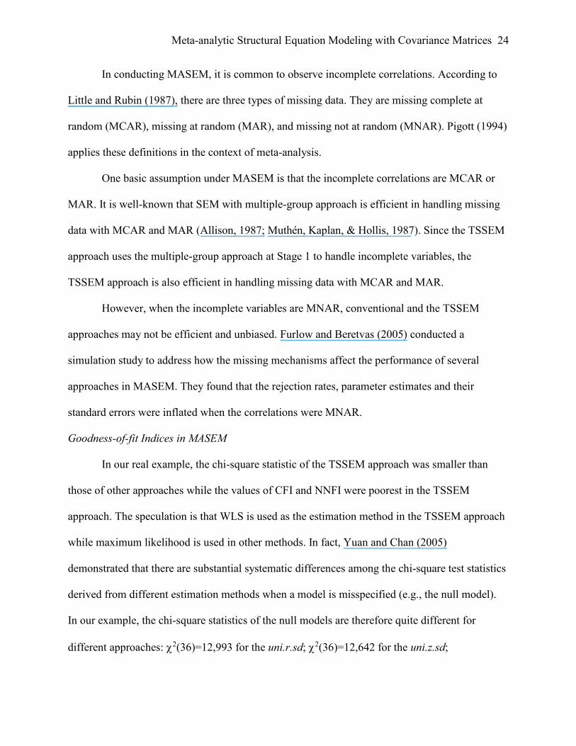
In conducting MASEM, it is common to observe incomplete correlations. According to

Little and Rubin (1987), there are three types of missing data. They are missing complete at

random (MCAR), missing at random (MAR), and missing not at random (MNAR). Pigott (1994)

applies these definitions in the context of meta-analysis.

One basic assumption under MASEM is that the incomplete correlations are MCAR or

MAR. It is well-known that SEM with multiple-group approach is efficient in handling missing

data with MCAR and MAR (Allison, 1987; Muthén, Kaplan, & Hollis, 1987). Since the TSSEM

approach uses the multiple-group approach at Stage 1 to handle incomplete variables, the

TSSEM approach is also efficient in handling missing data with MCAR and MAR.

However, when the incomplete variables are MNAR, conventional and the TSSEM

approaches may not be efficient and unbiased. Furlow and Beretvas (2005) conducted a

simulation study to address how the missing mechanisms affect the performance of several

approaches in MASEM. They found that the rejection rates, parameter estimates and their

standard errors were inflated when the correlations were MNAR.

Goodness-of-fit Indices in MASEM

In our real example, the chi-square statistic of the TSSEM approach was smaller than

those of other approaches while the values of CFI and NNFI were poorest in the TSSEM

approach. The speculation is that WLS is used as the estimation method in the TSSEM approach

while maximum likelihood is used in other methods. In fact, Yuan and Chan (2005)

demonstrated that there are substantial systematic differences among the chi-square test statistics

derived from different estimation methods when a model is misspecified (e.g., the null model).

In our example, the chi-square statistics of the null models are therefore quite different for

different approaches: 2(36)=12,993 for the uni.r.sd; 2(36)=12,642 for the uni.z.sd;

Meta-analytic Structural Equation Modeling with Covariance Matrices 25

2(36)=12,532 for the mul.r.sd; 2(36)=12,642 for the mul.z.sd; and 2(36)=4,083 for the

TSSEM approach. It is clear that the null model fits the data much better under the TSSEM

approach (or much poorer in other approaches). Since the null models are involved in calculating

many goodness-of-fit indices (e.g., Hu & Bentler, 1999; Rigdon, 1996), the CFI and NNFI of the

TSSEM approaches were poorer than those of other approaches. One more complication is that

there are two separate stages of analyses in MASEM. Further studies are required to address

which goodness-of-fit indices should be routinely recommended in MASEM.

Searching for Homogeneous Studies

Most studies in MASEM assume that the studies are homogeneous. If the studies are

heterogeneous, we may use cluster analysis to group the studies into relatively homogeneous

subgroups (M. W. L. Cheung & Chan, 2005b). It is relatively easy to extend the cluster analytic

approach to covariance matrices. Alternatively, we may consider the heterogeneity of studies

from the perspective of SEM by releasing some cross-group constraints to improve the model fit.

Hopefully, we may group the studies into several relatively homogeneous sub-groups. There are

several strategies on doing model modification in SEM, for instance, model modification indices

(Kaplan, 1990; MacCallum, 1986) and model specification searches (Marcoulides & Drezner,

2003; Marcoulides, Drezner, & Schumacker, 1998). Since it is possible to group the studies in

MASEM by searching for homogeneous variables or by searching for homogeneous studies,

further research is required to address how to apply these techniques properly in the context of

MASEM.

It has been recognized that many different statistical approaches can be well integrated

under the general latent variable modeling framework. For example, multilevel modeling (Bauer,

2003; Curran, 2003; Mehta & Neale, 2005), item response theory (Takane & DeLeeuw, 1987),

Meta-analytic Structural Equation Modeling with Covariance Matrices 26

generalized linear models (Skrondal & Rabe-Hesketh, 2004), and mixture models (Muthén,

2001). However, limited studies have addressed how to integrate SEM and meta-analysis into a

single framework (cf. M. W. L. Cheung, 2006; 2007b). The TSSEM approach and its extension

presented in this study hope to provide a start on this line of research.

Meta-analytic Structural Equation Modeling with Covariance Matrices 27

References

Allison, P. D. (1987). Estimation of linear models with incomplete data. Sociological

Methodology, 17, 71-103.

Bauer, D. J. (2003). Estimating multilevel linear models as structural equation models. Journal

of Educational and Behavioral Statistics, 28, 135-167.

Becker, B. J. (1992). Using results from replicated studies to estimate linear models. Journal of

Educational Statistics, 17, 341-362.

Becker, B. J. (1995). Corrections to “Using results from replicated studies to estimate linear

models”. Journal of Educational Statistics, 20, 100-102.

Becker, B. J. (2000). Multivariate meta-analysis. In H. E. A. Tinsley, & S. D. Brown (Eds.)

Handbook of applied multivariate statistics and mathematical modeling (pp.499-525).

San Diego: Academic Press.

Becker, B. J., & Fahrbach, K. (1994, April). A comparison of approaches to the synthesis of

correlation matrices. Paper presented at the annual meeting of the American Educational

Research Association, New Orleans, LA.

Becker, B. J., & Schram, C. M. (1994). Examining explanatory models through research

synthesis. In H. Cooper and L. V. Hedges (Eds). The handbook of research synthesis

(pp.357-381). New York: Russell Sage Foundation.

Becker, G. (1996). The meta-analysis of factor analyses: An illustration based on the cumulation

of correlation matrices. Psychological Methods, 1, 341-353.

Bentler, P. M. (1995). EQS structural equations program manual. Encino, CA: Multivariate

Software.

Meta-analytic Structural Equation Modeling with Covariance Matrices 28

Bentler, P. M., & Lee, S. Y. (1983). Covariance structure under polynomial constraints:

Application to correlation and Alpha-type structure models. Journal of Educational

Statistics, 8, 207-222.

Beretvas, S. N., & Furlow, C. F. (2006). Evaluation of an approximate method for synthesizing

covariance matrices for use in meta-analytic SEM. Structural Equation Modeling, 13,

153-185.

Bollen, K. A. (1989). Structural equations with latent variables. New York: Wiley.

Brown, S. P., & Peterson, R. A. (1993). Antecedents and consequences of salesperson job

satisfaction: Meta-analysis and assessment of causal effects. Journal of Marketing

Research, 30, 63-77.

Browne, M. W. (1984). Asymptotically distribution-free methods for the analysis of covariance

structures. British Journal of Mathematical and Statistical Psychology, 37, 62-83.

Browne, M. W., & Arminger, G. (1995). Specification and estimation of mean- and covariance-

structure models. In G. Arminger, C. C. Clogg, & M. E. Sobel (Eds.), Handbook of

statistical modeling for the social and behavioral sciences (pp. 185-249). New York:

Plenum Press.

Carson, P. P., Carson, K. D., & Roe, C. W. (1993). Social power bases: A meta-analytic

examination of interrelationships and outcomes. Journal of Applied Social Psychology,

23, 1150-1169.

Cheung, M. W. L. (2002). Meta-analysis for structural equation modeling: A two-stage

approach. Unpublished doctoral dissertation, Chinese University of Hong Kong, Hong

Kong.

Meta-analytic Structural Equation Modeling with Covariance Matrices 29

Cheung, M. W. L. (2006). Is meta-analysis a structural equation model? The case of fixed effects

models. Manuscript submitted for publication.

Cheung, M. W. L. (2007a). TSSEM: A LISREL syntax generator for two-stage structural

equation modeling (Version 1.10) [Computer software]. Retrieved from

http://courses.nus.edu.sg/course/psycwlm/internet/tssem.zip.

Cheung, M. W. L. (2007b). A general model for integrating fixed-, random-, and mixed-effects

meta-analyses into structural equation modeling. Manuscript submitted for publication.

Cheung, M. W. L. (in press). Constructing approximate confidence intervals for parameters with

structural equation models. Structural Equation Modeling.

Cheung, M. W. L., & Chan, W. (2004). Testing dependent correlation coefficients via structural

equation modeling. Organizational Research Methods, 7, 206-223.

Cheung, M. W. L., & Chan, W. (2005a). Meta-analytic structural equation modeling: A two-

stage approach. Psychological Methods, 10, 40-64.

Cheung, M. W. L., & Chan, W. (2005b). Classifying correlation matrices into relatively

homogeneous subgroups: A cluster analytic approach. Educational and Psychological

Measurement, 65, 954-979.

Cheung, M. W. L., Leung, K., & Au, K. (2006). Evaluating multilevel models in cross-cultural

research: An Illustration with Social Axioms. Journal of Cross-Cultural Psychology, 37,

522-541.

Cheung, S. F. (2000). Examining solutions to two practical issues in meta-analysis: Dependent

correlations and missing data in correlation matrices. Unpublished doctoral dissertation,

Chinese University of Hong Kong, Hong Kong.

Meta-analytic Structural Equation Modeling with Covariance Matrices 30

Colquitt, J. A., LePine, J. A., & Noe, R. A. (2000). Toward an integrative theory of training

motivation: A meta-analytic path analysis of 20 years of research. Journal of Applied

Psychology, 85, 678-707.

Conway, J. M. (1999). Distinguishing contextual performance from task performance for

managerial jobs. Journal of Applied Psychology, 84, 3-13.

Cudeck, R. (1989). Analysis of correlation matrices using covariance structure models.

Psychological Bulletin, 105, 317-327.

Curran, P. J. (2003). Have multilevel models been structural equation models all along?

Multivariate Behavioral Research, 38, 529-569.

Eby, L. T., Freeman, D. M., Rush, M. C., & Lance, C. E. (1999). Motivational bases of affective

organizational commitment: A partial test of an integrative theoretical model. Journal of

Occupational and Organizational Psychology, 72, 463-483.

Field, A. P. (2001). Meta-analysis of correlation coefficients: A Monte Carlo comparison of

fixed- and random-effects methods. Psychological Methods, 6, 161-180.

Fouladi, R. T. (2000). Performance of modified test statistics in covariance and correlation

structure analysis under conditions of multivariate nonnormality. Structural Equation

Modeling, 7, 356-410.

Furlow, C. F. &, Beretvas, S. N. (2005). Meta-analytic methods of pooling correlation matrices

for structural equation modeling under different patterns of missing data. Psychological

Methods, 10, 227-254.

Glass, G. V. (1976). Primary, secondary, and meta-analysis of research. Educational Researcher,

5, 3-8.

Meta-analytic Structural Equation Modeling with Covariance Matrices 31

Greenwald, A. G., Pratkanis, A. R., Leippe, M. R., & Baumgardner, M. H. (1986). Under what

conditions does theory obstruct research progress? Psychological Review, 93, 216-229.

Hafdahl, A. R. (2001). Multivariate meta-analysis for exploratory factor analytic research.

Unpublished doctoral dissertation, University of North Carolina at Chapel Hill.

Hedges, L. V., & Olkin, I. (1985). Statistical methods for meta-analysis. Orlando, FL: Academic

Press.

Hershberger, S. L. (2003). The growth of structural equation modeling: 1994-2001. Structural

Equation Modeling, 10, 35-46.

Hom, P. W., Caranikas-Walker, F., Prussia, G. E., & Griffeth, R. W. (1992). A meta-analytical

structural equations analysis of a model of employee turnover. Journal of Applied

Psychology, 77, 890-909.

Hoogland, J. J., & Boomsma, A. (1998). Robustness studies in covariance structure modeling:

An overview and a meta-analysis. Sociological Methods and Research, 26, 329-367.

Hu, L., & Bentler, P. M. (1999). Cutoff criteria for fit indexes in covariance structure analysis:

Conventional criteria versus new alternatives. Structural Equation Modeling, 6, 1-55.

Hunter, J. E. (1983). A causal analysis of cognitive ability, job knowledge, job performance, and

supervisor ratings. In F. Landy, S. Zedeck & J. Cleveland (Eds.) Performance

measurement and theory (pp.257-266). Hillsdale, N.J.: Lawrence Erlbaum Associates.

Hunter, J. E., & Hamilton, M. A. (2002). The advantages of using standardized scores in causal

analysis. Human Communication Research, 28, 552-561.

Hunter, J. E., & Schmidt, F. L. (2004). Methods of meta-analysis: Correcting error and bias in

research findings (2nd ed.). Thousand Oaks, Calif.: Sage.

Meta-analytic Structural Equation Modeling with Covariance Matrices 32

Inter-University Consortium for Political and Social Research (1989). International Social

Survey Program: Work Orientation. Ann Arbor, MI: Author.

Jöreskog, K. G. (2004). On Chi-squares for the independence model and fit measures in LISREL.

Retrieved from http://www.ssicentral.com/lisrel/techdocs/ftb.pdf.

Jöreskog, K. G., & Sörbom, D. (1996). LISREL 8: A user's reference guide. Chicago, IL:

Scientific Software International, Inc.

Jöreskog, K. G., & Sörbom, D (2006). LISREL 8.80 [Computer software]. Chicago, Ill.:

Scientific Software International.

Jöreskog, K. G., Sörbom, D., Du Toit, S., & Du Toit, M. (1999). LISREL 8: New Statistical

Features. Chicago, Ill.: Scientific Software International.

Kaplan, D. (1990). Evaluating and modifying covariance structure models: A review and

recommendation. Multivariate Behavioral Research, 25, 137-155.

Krane, W. R., & McDonald, R. P. (1978). Scale invariance and the factor analysis of correlation

matrices. British Journal of Mathematical and Statistical Psychology, 31, 218-228.

Little, R. J. A., & Rubin, D. B. (1987). Statistical analysis with missing data. New York: Wiley.

MacCallum, R. (1986). Specification searchers in covariance structure modeling. Psychological

Bulletin, 100, 107-120.

MacCallum, R. C., & Austin, J. T. (2000). Applications of structural equation modeling in

psychological research. Annual Review of Psychology, 51, 201-226.

Marcoulides, G. A., & Drezner, Z. (2003). Model specification searches using ant colony

optimization algorithms. Structural Equation Modeling, 10, 154-164.

Meta-analytic Structural Equation Modeling with Covariance Matrices 33

Marcoulides, G. A. Drezner, Z., & Schumacker, R. E. (1998). Model specification searches in

structural equation modeling using Tabu search. Structural Equation Modeling, 5, 365-

376.

Mehta, P. D., & Neale, M. C. (2005). People are variables too: Multilevel structural equation

modeling. Psychological Methods, 10, 259-284.

Muthén, B. (2001). Latent variable mixture modeling. In G. A. Marcoulides & R. E. Schumacker

(eds.), New Developments and Techniques in Structural Equation Modeling (pp. 1-33).

Lawrence Erlbaum Associates.

Muthén, B., Kaplan, D., & Hollis, M. (1987). On structural equation modeling with data that are

not missing completely at random. Psychometrika, 51, 431-462.

National Research Council (1992). Combining information: Statistical issues and opportunities

for research. Washington, D.C.: National Academy Press.

Neale, M.C., Boker, S. M., Xie, G., & Maes, H. H. (2006). Mx: Statistical modeling (7th ed.).

VCU Box 900126, Richmond, VA 23298: Department of Psychiatry.

Pigott, T. D. (1994). Methods for handling missing data in research synthesis. In H. Cooper and

L. V. Hedges (Eds). The handbook of research synthesis (pp.163-175). New York:

Russell Sage Foundation.

Premack, S. L., & Hunter, J. E. (1988). Individual unionization decisions. Psychological Bulletin,

103, 223-234.

R Development Core Team (2007). R: A language and environment for statistical computing. R

Foundation for Statistical Computing, Vienna, Austria. ISBN 3-900051-07-0, URL:

http://www.r-project.org.

Meta-analytic Structural Equation Modeling with Covariance Matrices 34

Raykov, T. (2001). Testing multivariate covariance structure and means hypotheses via structural

equation modeling. Structural Equation Modeling, 8, 224-256.

Raudenbush, S. W., Becker, B. J., & Kalaian, H. (1988). Modeling multivariate effect sizes.

Psychological Bulletin, 103, 111-120.

Raudenbush, S. W., & Bryk, A. S. (2002). Hierarchical linear models: Applications and data

analysis methods (2nd Ed.). Thousand Oaks, CA: Sage Publications.

Rigdon, E. E. (1996). CFI versus RMSEA: A comparison of two fit indexes for structural

equation modeling. Structural Equation Modeling, 3, 369-379.

Schmidt, F. L., Hunter, J. E., & Outerbridge, A. N. (1986). Impact of job experience and ability

on job knowledge, work sample performance, and supervisory ratings of job performance.

Journal of Applied Psychology, 71, 432-439.

Shadish, W.R. (1996). Meta-analysis and the exploration of causal mediating processes: A

primer of examples, methods, and issues. Psychological Methods, 1, 47-65.

Skrondal, A., & Rabe-Hesketh, S. (2004). Generalized latent variable modeling: Multilevel,

longitudinal, and structural equation models. Boca Raton: Chapman & Hall.

Steiger, J. H. (1980). Tests for comparing elements of a correlation matrix. Psychological

Bulletin, 87, 245-251.

Takane, Y. & DeLeeuw, J. (1987). On the relationship between item response theory and factor

analysis of discretized variables. Psychometrika, 52, 393-408.

Tett, R. P., & Meyer, J. P. (1993). Job satisfaction, organizational commitment, turnover

intention, and turnover: Path analyses based on meta-analytic findings. Personnel

Psychology, 46, 259-290.

Meta-analytic Structural Equation Modeling with Covariance Matrices 35

Tremblay, P. F., & Gardner, R. C. (1996). On the growth of structural equation modeling in

psychological journals. Structural Equation Modeling, 7, 629-636.

Verhaeghen, P., & Salthouse, T. A. (1997). Meta-analyses of age-cognition relations in

adulthood: Estimates of linear and nonlinear age effects and structural models.

Psychological Bulletin, 122, 231-249.

Viswesvaran, C., & Ones, D. S. (1995). Theory testing: Combining psychometric meta-analysis

and structural equations modeling. Personnel Psychology, 48, 865-885.

Yuan, K.-H., & Chan, W. (2005). On nonequivalence of several procedures of structural

equation modeling. Psychometrika, 70, 791-798.

Meta-analytic Structural Equation Modeling with Covariance Matrices 36

Author Note

Mike W.-L. Cheung, Department of Psychology, National University of Singapore; Wai

Chan, Department of Psychology, Chinese University of Hong Kong.

This research was supported by the Academic Research Fund Tier 1 (R-581-000-064-112)

from the Ministry of Education, Singapore. We would like to thank Kevin Au for sharing with us

information about International Social Survey Program data set.

Correspondence concerning this article should be addressed to Mike W.-L. Cheung,

Department of Psychology, Faculty of Arts and Social Sciences, National University of

Singapore, Block AS4, Level 2, 9 Arts Link, Singapore 117570. Tel: (65) 6516-3702; Fax: (65)

6773-1843; E-mail: mikewlcheung@nus.edu.sg.

Meta-analytic Structural Equation Modeling with Covariance Matrices 37

Endnotes

1The weight )()( ggr nw is sometimes used instead of 22)()()( ))(1/( g

ijgg

r rnw in pooling

correlations (see Field, 2001; Hunter & Schmidt, 2004).

2With any consistent weight matrix, the test statistic T follows a chi-square distribution

with (p*-q) degrees of freedom in large samples, that is,

)*(~)()1( 2min qpFnT θ

where )(min θF is the minimum of )(θF in Equation 16, n is the sample size and q is the number

of free parameters estimated when the model is correctly specified (Browne, 1984). For the ease

of discussion, we use n instead of (n-1) in this paper. After the Stage 1 analysis, we have a 1*p

vector of covariances *s and its ** pp asymptotic covariance matrix V . The total sample

size

K

g

gnN1

)( is used as the sample size in the Stage 2 analysis. Since N is multiplied into V ,

which is inverted in Equation 16, the effect of the sample size is cancelled out as shown by

))(*()ˆ())(*( 1T θθ sVNsN .

Alternatively, it is also possible not to multipliy N into V and to use N=1 in the Stage 2

analysis. When N=1 is used in LISREL, the sample size is simply not included in the fit function.

It can be verified empirically that the test statistics, parameter estimates and their standard errors

are equivalent in both approaches (within round-off errors). Since the sample size is explicitly

involved in calculating some goodness-of-fit indices, using N=1 may result in incorrect

goodness-of-fit indices. Therefore, we suggest multiplying N into V and using the total sample

size in the analysis.

3Some of the goodness-of-fit indices for the correlation matrices are slightly different

from those reported in M. W. L. Cheung and Chan (2005a). The reason is that LISREL 8.80 was

Meta-analytic Structural Equation Modeling with Covariance Matrices 38

used in this study while LISREL 8.30 was used in M. W. L. Cheung and Chan (2005a). Started

from LISREL 8.70, some formulas in calculating the chi-square statistics and the goodness-of-fit

indices were changed (Jöreskog, 2004).

Meta-analytic Structural Equation Modeling with Covariance Matrices 39

Table 1

Rejection Percentages with = .05 of Stages 1 and 2 Analyses

Population standard deviation

No. of studies

Average N per study

uni.r.sd uni.z.sd mul.r.sd mul.z.sd TSSEM

Stage 1: Testing homogeneity of covariance matrices 1.0 10 100 0.205** 0.110** 0.145** 0.065 0.040

300 0.140** 0.120** 0.074** 0.056 0.048 1,000 0.106** 0.096** 0.062 0.058 0.042 20 100 0.270** 0.119** 0.166** 0.074** 0.054 300 0.162** 0.112** 0.087** 0.062 0.050 1,000 0.106** 0.095** 0.055 0.051 0.043 30 100 0.299** 0.127** 0.217** 0.073** 0.055 300 0.166** 0.112** 0.111** 0.061 0.051 1,000 0.122** 0.108** 0.073** 0.065 0.055

3.0 10 100 0.184** 0.094** 0.120** 0.059 0.046 300 0.141** 0.120** 0.075** 0.059 0.044 1,000 0.111** 0.108** 0.056 0.051 0.045 20 100 0.243** 0.107** 0.157** 0.062 0.035* 300 0.148** 0.112** 0.097** 0.066* 0.059 1,000 0.134** 0.127** 0.075** 0.067* 0.048 30 100 0.321** 0.121** 0.216** 0.073** 0.050 300 0.154** 0.118** 0.106** 0.072** 0.063 1,000 0.106** 0.092** 0.060 0.048 0.044 Stage 2: Fitting confirmatory factor analytic models

1.0 10 100 0.101** 0.060 0.046 0.060 0.049 300 0.061 0.050 0.048 0.050 0.045 1,000 0.050 0.047 0.046 0.047 0.044 20 100 0.078** 0.053 0.042 0.053 0.045 300 0.078** 0.072** 0.069* 0.072** 0.062 1,000 0.060 0.061 0.061 0.061 0.059 30 100 0.085** 0.050 0.044 0.050 0.041 300 0.063 0.054 0.049 0.054 0.051 1,000 0.057 0.055 0.054 0.055 0.053

3.0 10 100 0.091** 0.063 0.054 0.063 0.055 300 0.061 0.053 0.051 0.053 0.046 1,000 0.057 0.054 0.053 0.054 0.053 20 100 0.103** 0.059 0.051 0.059 0.049 300 0.058 0.046 0.044 0.046 0.042 1,000 0.046 0.042 0.042 0.042 0.041 30 100 0.085** 0.054 0.041 0.054 0.043 300 0.059 0.055 0.054 0.055 0.052 1,000 0.057 0.053 0.052 0.053 0.048

Note. uni.r.sd = univariate approach to synthesizing correlations and standard deviations; uni.z.sd

= univariate approach to synthesizing Fisher’s z scores and standard deviations; mul.r.sd =

Meta-analytic Structural Equation Modeling with Covariance Matrices 40

multivariate approach to synthesizing correlations and standard deviations; mul.z.sd =

multivariate approach to synthesizing Fisher’s z scores and standard deviations; TSSEM = two-

stage structural equation modeling approach in pooling covariance matrices. * Rejection

percentage falls outside the 95% acceptance regions. ** Rejection percentage falls outside the

99% acceptance regions.

Meta-analytic Structural Equation Modeling with Covariance Matrices 41

Table 2

Relative Percentage Bias of Parameter Estimates in Stage 2

Average N per study

Methods 11 21 31 21 11 22 33

No. of studies=10 100 uni.r.sd 1.17 1.16 1.63 0.95 -4.65 -2.29 -1.72

uni.z.sd 0.24 0.11 0.37 0.23 -1.32 -0.25 -0.29 mul.r.sd -0.07 -0.23 -0.04 -0.01 -0.23 0.41 0.18 mul.z.sd 0.24 0.11 0.37 0.23 -1.32 -0.25 -0.29 TSSEM -0.05 -0.16 0.03 0.62 -1.34 -0.57 -0.72

300 uni.r.sd 0.41 0.24 0.37 0.21 -1.56 -0.55 -0.46 uni.z.sd 0.10 -0.10 -0.04 -0.03 -0.48 0.10 0.00 mul.r.sd 0.00 -0.21 -0.18 -0.10 -0.12 0.32 0.16 mul.z.sd 0.10 -0.10 -0.04 -0.03 -0.48 0.10 0.00 TSSEM 0.00 -0.19 -0.15 0.09 -0.49 -0.01 -0.12

1,000 uni.r.sd 0.09 0.15 0.20 0.31 -0.34 -0.24 -0.14 uni.z.sd 0.01 0.05 0.07 0.24 -0.03 -0.06 0.00 mul.r.sd -0.02 0.02 0.03 0.22 0.07 0.00 0.04 mul.z.sd 0.01 0.05 0.07 0.24 -0.03 -0.06 0.00 TSSEM -0.02 0.02 0.04 0.28 -0.03 -0.09 -0.04 No. of studies=20

100 uni.r.sd 1.13 1.28 1.30 1.12 -4.19 -2.71 -1.71 uni.z.sd 0.19 0.20 -0.05 0.30 -0.83 -0.61 -0.18 mul.r.sd -0.12 -0.15 -0.49 0.05 0.27 0.06 0.31 mul.z.sd 0.19 0.20 -0.05 0.30 -0.83 -0.61 -0.18 TSSEM -0.03 -0.02 -0.33 0.40 -0.56 -0.56 -0.25

Note. uni.r.sd = univariate approach to synthesizing correlations and standard deviations; uni.z.sd = univariate approach to synthesizing Fisher’s z scores and standard deviations; mul.r.sd = multivariate approach to synthesizing correlations and standard deviations; mul.z.sd = multivariate approach to synthesizing Fisher’s z scores and standard deviations; TSSEM = two-stage structural equation modeling approach in pooling covariance matrices.

Meta-analytic Structural Equation Modeling with Covariance Matrices 42

Table 2 (continued) Average N per

study Methods

11 21 31 21 11 22 33

300 uni.r.sd 0.46 0.45 0.55 0.40 -1.53 -0.89 -0.58 uni.z.sd 0.15 0.10 0.12 0.15 -0.41 -0.22 -0.09 mul.r.sd 0.04 -0.01 -0.03 0.06 -0.04 0.00 0.07 mul.z.sd 0.15 0.10 0.12 0.15 -0.41 -0.22 -0.09 TSSEM 0.06 0.02 0.02 0.17 -0.31 -0.21 -0.11

1,000 uni.r.sd 0.05 0.13 0.10 0.02 -0.33 -0.25 -0.16 uni.z.sd -0.04 0.03 -0.03 -0.05 0.00 -0.05 -0.01 mul.r.sd -0.07 -0.01 -0.07 -0.08 0.11 0.02 0.04 mul.z.sd -0.04 0.03 -0.03 -0.05 0.00 -0.05 -0.01 TSSEM -0.06 0.00 -0.06 -0.04 0.03 -0.04 -0.02 No. of studies=30

100 uni.r.sd 1.09 1.19 1.55 0.69 -4.14 -2.51 -1.86 uni.z.sd 0.10 0.08 0.19 -0.11 -0.60 -0.36 -0.32 mul.r.sd -0.22 -0.28 -0.26 -0.36 0.56 0.33 0.18 mul.z.sd 0.10 0.08 0.19 -0.11 -0.60 -0.36 -0.32 TSSEM -0.10 -0.13 -0.06 -0.07 -0.25 -0.22 -0.29

300 uni.r.sd 0.36 0.34 0.39 0.36 -1.42 -0.84 -0.52 uni.z.sd 0.05 -0.02 -0.05 0.10 -0.31 -0.14 -0.02 mul.r.sd -0.05 -0.14 -0.20 0.01 0.06 0.08 0.14 mul.z.sd 0.05 -0.02 -0.05 0.10 -0.31 -0.14 -0.02 TSSEM -0.02 -0.09 -0.13 0.11 -0.17 -0.11 -0.02

1,000 uni.r.sd 0.08 0.13 0.08 0.03 -0.36 -0.27 -0.14 uni.z.sd -0.02 0.02 -0.05 -0.05 -0.01 -0.06 0.01 mul.r.sd -0.05 -0.01 -0.10 -0.07 0.10 0.01 0.06 mul.z.sd -0.02 0.02 -0.05 -0.05 -0.01 -0.06 0.01 TSSEM -0.03 0.00 -0.08 -0.04 0.02 -0.04 0.01

Meta-analytic Structural Equation Modeling with Covariance Matrices 43

Table 3

Relative Percentage Bias of Standard Errors of Parameter Estimates in Stage 2

Average N per study

Methods 11 21 31 21 11 22 33

No. of studies=10 100 Uni.r.sd -5.41 -2.63 -4.18 -6.75 -6.04 -6.66 -4.25

Uni.z.sd -3.10 -0.51 -1.25 -4.46 0.10 -2.20 -1.23 Mul.r.sd -2.89 -0.47 -0.83 -3.85 0.95 -1.74 -0.95 Mul.z.sd -3.10 -0.51 -1.25 -4.46 0.10 -2.20 -1.23 TSSEM -2.46 0.39 -0.17 -3.59 0.92 -0.87 -0.41

300 Uni.r.sd -1.98 1.01 -4.80 -0.32 -2.63 -4.18 -3.65 Uni.z.sd -1.06 1.59 -3.97 0.49 -0.95 -2.95 -2.78 Mul.r.sd -0.93 1.60 -3.82 0.70 -0.77 -2.87 -2.68 Mul.z.sd -1.06 1.59 -3.97 0.49 -0.95 -2.95 -2.78 TSSEM -0.66 1.80 -3.70 1.07 -0.91 -2.72 -2.67

1,000 Uni.r.sd -4.07 3.71 1.15 1.93 -3.37 1.66 -1.26 Uni.z.sd -3.79 4.08 1.36 2.24 -2.95 2.07 -0.69 Mul.r.sd -3.75 4.15 1.37 2.34 -2.91 2.11 -0.56 Mul.z.sd -3.79 4.08 1.36 2.24 -2.95 2.07 -0.69 TSSEM -3.74 4.30 1.63 2.44 -2.86 2.30 -0.64 No. of studies=20

100 Uni.r.sd -6.76 -2.80 -6.79 -7.82 -8.55 -8.11 -6.56 Uni.z.sd -3.74 -0.36 -3.96 -5.35 -1.48 -3.08 -3.01 Mul.r.sd -3.29 -0.22 -3.48 -4.65 -0.37 -2.58 -2.54 Mul.z.sd -3.74 -0.36 -3.96 -5.35 -1.48 -3.08 -3.01 TSSEM -2.00 0.54 -3.26 -4.42 -0.05 -1.89 -1.74

Note. uni.r.sd = univariate approach to synthesizing correlations and standard deviations; uni.z.sd = univariate approach to synthesizing Fisher’s z scores and standard deviations; mul.r.sd = multivariate approach to synthesizing correlations and standard deviations; mul.z.sd = multivariate approach to synthesizing Fisher’s z scores and standard deviations; TSSEM = two-stage structural equation modeling approach in pooling covariance matrices.

Meta-analytic Structural Equation Modeling with Covariance Matrices 44

Table 3 (continued) Average N per

study Methods

11 21 31 21 11 22 33

300 Uni.r.sd -0.80 -1.68 -0.80 -3.03 -5.08 -4.35 -2.46 Uni.z.sd 0.10 -0.28 0.24 -2.40 -3.02 -2.21 -0.61 Mul.r.sd 0.21 0.02 0.39 -2.22 -2.70 -1.76 -0.19 Mul.z.sd 0.10 -0.28 0.24 -2.40 -3.02 -2.21 -0.61 TSSEM 1.03 -0.07 0.53 -1.89 -2.19 -1.37 -0.03

1,000 Uni.r.sd 7.15 1.81 3.44 1.34 3.64 -0.81 4.88 Uni.z.sd 7.36 2.02 3.73 1.49 4.21 -0.51 5.21 Mul.r.sd 7.34 2.02 3.76 1.54 4.26 -0.52 5.24 Mul.z.sd 7.36 2.02 3.73 1.49 4.21 -0.51 5.21 TSSEM 7.48 2.12 3.76 1.46 4.25 -0.50 5.19 No. of studies=30

100 Uni.r.sd -5.69 -3.85 -1.10 -1.14 -6.65 -8.26 -2.80 Uni.z.sd -2.74 -0.75 1.90 1.45 -0.18 -2.46 1.18 Mul.r.sd -2.42 -0.37 2.22 2.14 0.64 -1.65 1.69 Mul.z.sd -2.74 -0.75 1.90 1.45 -0.18 -2.46 1.18 TSSEM -1.17 1.22 3.24 2.70 1.68 -0.79 2.82

300 Uni.r.sd -1.44 -4.81 1.84 2.60 -0.29 -3.01 -3.64 Uni.z.sd -0.18 -3.94 2.79 3.32 2.18 -1.49 -2.17 Mul.r.sd 0.03 -3.83 2.91 3.56 2.58 -1.33 -1.94 Mul.z.sd -0.18 -3.94 2.79 3.32 2.18 -1.49 -2.17 TSSEM 0.39 -3.45 3.10 3.59 2.93 -0.62 -1.78

1,000 Uni.r.sd 1.17 -2.03 -2.32 -2.64 -0.52 -0.84 1.40 Uni.z.sd 1.49 -1.59 -2.15 -2.46 0.09 0.33 1.82 Mul.r.sd 1.52 -1.51 -2.15 -2.40 0.17 0.61 1.90 Mul.z.sd 1.49 -1.59 -2.15 -2.46 0.09 0.33 1.82 TSSEM 1.68 -1.53 -1.98 -2.44 0.26 0.44 1.82

Meta-analytic Structural Equation Modeling with Covariance Matrices 45

Table 4

Goodness-of-fit Indices of the Real Example

uni.r.sd uni.z.sd mul.r.sd mul.z.sd TSSEM

Stage 1: Testing homogeneity of covariance matrices

2 (df) 2,809 (450) 2,775 (450) 2,225 (450) 2,226 (450) 2,510 (450)

Stage 1: Testing homogeneity of correlation matrices

2 (df) 1,275 (360) 1,241 (360) 948 (360) 945 (360) 941 (360)

Stage 1: Testing homogeneity of variances

2 (df) 1,534 (90)a 1,534 (90)a 1,278 (90) 1,281 (90) 1,216 (90)

Stage 2: Fitting a confirmatory factor analytic model

2 (df) 1,860 (24) 1,808 (24) 1,792 (24) 1,808 (24) 1,164 (24)

CFI 0.87 0.87 0.87 0.87 0.72

NNFI 0.81 0.81 0.81 0.81 0.58

RMSEA 0.10 0.10 0.10 0.10 0.08

SRMR 0.06 0.06 0.06 0.06 0.07

Note. uni.r.sd = univariate approach to pooling correlations and standard deviations; uni.z.sd =

univariate approach to pooling Fisher’s z scores and standard deviations; mul.r.sd = multivariate

approach to pooling correlations and standard deviations; mul.z.sd = multivariate approach to

pooling Fisher’s z scores and standard deviations; TSSEM = two-stage structural equation

modeling approach in pooling covariance matrices. 2(df) = Chi-square test statistic and its

associated degrees of freedom; CFI = Comparative Fit Index; NNFI = Non-Normed Fit Index;

RMSEA = Root Mean Square Error of Approximation; SRMR = Standardized Root Mean

Square Residual. aThe univariate methods of pooling standard deviations were the same.

Meta-analytic Structural Equation Modeling with Covariance Matrices 46

Table 5

Parameter Estimates and Their Standard Errors of the Real Example

Parameter Estimates uni.r.sd uni.z.sd mul.r.sd mul.z.sd TSSEM

11 0.45 (0.01) 0.45 (0.01) 0.45 (0.02) 0.45 (0.01) 0.47 (0.02)

21 0.64 (0.02) 0.64 (0.02) 0.63 (0.02) 0.64 (0.02) 0.58 (0.02)

31 0.69 (0.02) 0.68 (0.02) 0.68 (0.02) 0.68 (0.02) 0.64 (0.02)

42 0.58 (0.01) 0.58 (0.01) 0.58 (0.01) 0.58 (0.01) 0.60 (0.01)

52 0.47 (0.01) 0.47 (0.01) 0.47 (0.01) 0.47 (0.01) 0.49 (0.01)

62 0.70 (0.01) 0.69 (0.01) 0.69 (0.01) 0.69 (0.01) 0.70 (0.01)

72 0.62 (0.01) 0.61 (0.01) 0.61 (0.01) 0.61 (0.01) 0.62 (0.01)

83 0.75 (0.04) 0.72 (0.04) 0.72 (0.04) 0.72 (0.04) 0.73 (0.04)

93 0.33 (0.02) 0.32 (0.02) 0.32 (0.02) 0.32 (0.02) 0.32 (0.02)

21 0.39 (0.02) 0.39 (0.02) 0.39 (0.02) 0.39 (0.02) 0.47 (0.02)

31 0.42 (0.03) 0.43 (0.03) 0.43 (0.03) 0.43 (0.03) 0.40 (0.03)

32 0.35 (0.03) 0.37 (0.03) 0.37 (0.03) 0.37 (0.03) 0.39 (0.03)

11 0.88 (0.02) 0.88 (0.02) 0.88 (0.02) 0.88 (0.02) 0.86 (0.02)

22 0.57 (0.02) 0.58 (0.02) 0.58 (0.02) 0.58 (0.02) 0.58 (0.02)

33 0.65 (0.02) 0.66 (0.02) 0.66 (0.02) 0.66 (0.02) 0.66 (0.02)

44 0.51 (0.01) 0.51 (0.01) 0.51 (0.01) 0.51 (0.01) 0.45 (0.01)

55 0.70 (0.01) 0.70 (0.01) 0.70 (0.01) 0.70 (0.01) 0.62 (0.01)

66 0.56 (0.01) 0.57 (0.01) 0.57 (0.01) 0.57 (0.01) 0.52 (0.01)

77 0.54 (0.01) 0.54 (0.01) 0.55 (0.01) 0.54 (0.01) 0.47 (0.01)

88 1.12 (0.06) 1.15 (0.06) 1.16 (0.06) 1.15 (0.06) 1.05 (0.06)

99 0.99 (0.02) 1.00 (0.02) 1.00 (0.02) 1.00 (0.02) 0.98 (0.02) Note. Note. uni.r.sd = univariate approach to synthesizing correlations and standard deviations;

uni.z.sd = univariate approach to synthesizing Fisher’s z scores and standard deviations; mul.r.sd

= multivariate approach to synthesizing correlations and standard deviations; mul.z.sd =

multivariate approach to synthesizing Fisher’s z scores and standard deviations; TSSEM = two-

stage structural equation modeling approach in pooling covariance matrices.

Meta-analytic Structural Equation Modeling with Covariance Matrices 47

Appendix

LISREL syntax to testing the homogeneity of covariance matrices, the homogeneity of

correlation matrices, and the homogeneity of variances

! In analyzing the real data, 11 groups were involved. ! To save journal space, only 2 groups are listed here. TI TSSEM Stage 1: Testing the homogeneity of covariance matrices DA NG=2 NI=9 NO=591 CM FU FI=covariance.dat MO NX=9 NK=9 LX=ID TD=ZE PH=SY,FR OU TI TSSEM Stage 1: Group 2 DA NI=9 NO=656 CM FU FI=covariance.dat MO NX=9 NK=9 LX=ID TD=ZE PH=SY,FR ! Constraints on testing the homogeneity of variances EQ PH(1,1,1) PH(2,1,1) EQ PH(1,2,2) PH(2,2,2) EQ PH(1,3,3) PH(2,3,3) EQ PH(1,4,4) PH(2,4,4) EQ PH(1,5,5) PH(2,5,5) EQ PH(1,6,6) PH(2,6,6) EQ PH(1,7,7) PH(2,7,7) EQ PH(1,8,8) PH(2,8,8) EQ PH(1,9,9) PH(2,9,9) ! Constraints on testing the homogeneity of covariances EQ PH(1,1,2) PH(2,1,2) EQ PH(1,1,3) PH(2,1,3) EQ PH(1,1,4) PH(2,1,4) EQ PH(1,1,5) PH(2,1,5) EQ PH(1,1,6) PH(2,1,6) EQ PH(1,1,7) PH(2,1,7) EQ PH(1,1,8) PH(2,1,8) EQ PH(1,1,9) PH(2,1,9) EQ PH(1,2,3) PH(2,2,3) EQ PH(1,2,4) PH(2,2,4) EQ PH(1,2,5) PH(2,2,5) EQ PH(1,2,6) PH(2,2,6) EQ PH(1,2,7) PH(2,2,7) EQ PH(1,2,8) PH(2,2,8) EQ PH(1,2,9) PH(2,2,9) EQ PH(1,3,4) PH(2,3,4) EQ PH(1,3,5) PH(2,3,5) EQ PH(1,3,6) PH(2,3,6) EQ PH(1,3,7) PH(2,3,7) EQ PH(1,3,8) PH(2,3,8) EQ PH(1,3,9) PH(2,3,9) EQ PH(1,4,5) PH(2,4,5)

Meta-analytic Structural Equation Modeling with Covariance Matrices 48

EQ PH(1,4,6) PH(2,4,6) EQ PH(1,4,7) PH(2,4,7) EQ PH(1,4,8) PH(2,4,8) EQ PH(1,4,9) PH(2,4,9) EQ PH(1,5,6) PH(2,5,6) EQ PH(1,5,7) PH(2,5,7) EQ PH(1,5,8) PH(2,5,8) EQ PH(1,5,9) PH(2,5,9) EQ PH(1,6,7) PH(2,6,7) EQ PH(1,6,8) PH(2,6,8) EQ PH(1,6,9) PH(2,6,9) EQ PH(1,7,8) PH(2,7,8) EQ PH(1,7,9) PH(2,7,9) EQ PH(1,8,9) PH(2,8,9) ! Output the pooled covariance matrix ! and its asymptotic covariance matrix OU PH=cov1.cor EC=cov1.ack TI TSSEM Stage 2: Fitting a CFA based on the pooled covariance matrix DA NI=9 NO=7155 MA=CM ! The elements for cov2.cor and cov2.ack are ! calculated from cov1.cor and cov1.ack. ! A DOS program to conduct the computations ! can be obtained from the first author’s website. CM=cov2.cor SY AC=cov2.ack SY MO NX=9 NK=3 PH=ST,FR PA LX 3*(1 0 0) 4*(0 1 0) 2*(0 0 1) ! Weighted least squares is required as the estimation method OU ME=WL TI TSSEM Stage 1: Testing the homogeneity of correlation matrices DA NG=2 NI=9 NO=591 CM FU FI=covariance.dat MO NX=9 NK=9 LX=DI,FR TD=ZE PH=ST,FR OU TI TSSEM Stage 1: Group 2 DA NI=9 NO=656 CM FU FI=covariance.dat MO NX=9 NK=9 LX=DI,FR TD=ZE PH=ST,FR ! Constraints on testing the homogeneity of correlation matrices EQ PH(1,1,2) PH(2,1,2) EQ PH(1,1,3) PH(2,1,3) EQ PH(1,1,4) PH(2,1,4) EQ PH(1,1,5) PH(2,1,5) EQ PH(1,1,6) PH(2,1,6) EQ PH(1,1,7) PH(2,1,7) EQ PH(1,1,8) PH(2,1,8) EQ PH(1,1,9) PH(2,1,9) EQ PH(1,2,3) PH(2,2,3) EQ PH(1,2,4) PH(2,2,4)

Meta-analytic Structural Equation Modeling with Covariance Matrices 49

EQ PH(1,2,5) PH(2,2,5) EQ PH(1,2,6) PH(2,2,6) EQ PH(1,2,7) PH(2,2,7) EQ PH(1,2,8) PH(2,2,8) EQ PH(1,2,9) PH(2,2,9) EQ PH(1,3,4) PH(2,3,4) EQ PH(1,3,5) PH(2,3,5) EQ PH(1,3,6) PH(2,3,6) EQ PH(1,3,7) PH(2,3,7) EQ PH(1,3,8) PH(2,3,8) EQ PH(1,3,9) PH(2,3,9) EQ PH(1,4,5) PH(2,4,5) EQ PH(1,4,6) PH(2,4,6) EQ PH(1,4,7) PH(2,4,7) EQ PH(1,4,8) PH(2,4,8) EQ PH(1,4,9) PH(2,4,9) EQ PH(1,5,6) PH(2,5,6) EQ PH(1,5,7) PH(2,5,7) EQ PH(1,5,8) PH(2,5,8) EQ PH(1,5,9) PH(2,5,9) EQ PH(1,6,7) PH(2,6,7) EQ PH(1,6,8) PH(2,6,8) EQ PH(1,6,9) PH(2,6,9) EQ PH(1,7,8) PH(2,7,8) EQ PH(1,7,9) PH(2,7,9) EQ PH(1,8,9) PH(2,8,9) ! Output the pooled correlation matrix ! and its asymptotic covariance matrix OU PH=cor1.cor EC=cor1.ack TI TSSEM Stage 2: Fitting a CFA based on the pooled correlation matrix DA NI=9 NO=7155 MA=KM ! The elements for cor2.cor and cor2.ack are ! calculated from cor1.cor and cor1.ack. ! A DOS program to conduct the computations ! can be obtained from the first author’s website. KM=cor2.cor SY AC=cor2.ack SY MO NX=9 NK=3 PH=ST,FR PA LX 3*(1 0 0) 4*(0 1 0) 2*(0 0 1) ! Weighted least squares is required as the estimation method OU ME=WL TI TSSEM Stage 1: Testing the homogeneity of variances DA NG=2 NI=9 NO=591 CM FU FI=covariance.dat MO NX=9 NK=9 LX=ID TD=ZE PH=SY,FR OU TI TSSEM Stage 1: Group 2 DA NI=9 NO=656 CM FU FI=covariance.dat

Meta-analytic Structural Equation Modeling with Covariance Matrices 50

MO NX=9 NK=9 LX=ID TD=ZE PH=SY,FR ! Constraints on testing the homogeneity of variances EQ PH(1,1,1) PH(2,1,1) EQ PH(1,2,2) PH(2,2,2) EQ PH(1,3,3) PH(2,3,3) EQ PH(1,4,4) PH(2,4,4) EQ PH(1,5,5) PH(2,5,5) EQ PH(1,6,6) PH(2,6,6) EQ PH(1,7,7) PH(2,7,7) EQ PH(1,8,8) PH(2,8,8) EQ PH(1,9,9) PH(2,9,9) OU