The Trillion Dollar Conundrum: Complementarities and Health Information Technology
A Two-Country NATREX Model for the Euro/Dollar:
Theoretical Approach
Marianna Belloc and Daniela Federici�
CIDEI Working paper No. 76 - April 2007
Abstract
This paper develops a NATREX (NATural Real EXchange rate) model for two large economies,
the Eurozone and the United States. The NATREX approach has already been adopted to
explain the medium-long term dynamics of the real exchange rate in a number of industrial
countries. So far, however, it has been applied to a one-country framework where the �rest
of the world� is treated as given. In this paper, we build a NATREX model where the two
economies are fully speci�ed and allowed to interact. Our theoretical model o¤ers the basis to
empirical estimation of the euro/dollar equilibrium exchange rate that will be carried out in
future research.
Key words : NATREX; equilibrium exchange rate; euro/dollar; structural approach
JEL classi�cation : F31; F36; F47
�Marianna Belloc: Department of Economics and CIDEI, Sapienza University of Rome (Italy).
Email: [email protected]. Daniela Federici: Department of Economics, University of Cassino (Italy).
Email: [email protected]. We are indebted to Giancarlo Gandolfo for many generous comments and suggestions.
The usual disclaimer applies.
1
1 Introduction
Since the introduction of the euro as common currency for 11 member states of the EU, the
euro-dollar exchange rate has surprised most observers for its highly unexpected dynamics.
As �gure 1 shows, it has depreciated steadily and almost continuously from January 1999 to
February 2002, then it reversed this trend, began to rise and kept doing so until December
2004. Thereafter the euro has substantially stabilized at a high level with respect to the
US dollar. The study of such an anomalous behavior has given rise to a growing literature
that looks for theoretically coherent explanations. They include black market holdings of
euros (Sinn and Westermann, 2001); reactions to �scal policy (Cohen and Loisel, 2000);
responses to fundamental variables such as productivity di¤erentials (e.g. Alquist and
Chinn 2002, Bailey et al. 2001), growth rate of money, per capita income, population and
capital accumulation (Welfens, 2001); in�ation di¤erentials, relative rates of return of US
versus Euroland assets, current account (e.g. De Grauwe, 2000, De Grauwe and Grimaldi,
2005. For a survey see Shams, 2005). Despite the large number of studies on the issue,
however, the state of the art does not seem to have reached any satisfactory arrival point: the
behavior of the euro-dollar between 1999 and 2004 remains mostly puzzling to the economic
theory. Yet, understanding what drives the euro-dollar real exchange rate developments is
crucial for both theoretical and policy implications. In this paper we look at the issue from
a di¤erent perspective. Rather than trying to explain the actual real exchange rate (RER),
we study the determinants of the real equilibrium exchange rate (REER) of the euro/dollar
in order to provide a yardstick against which the development of the actual real exchange
rate is gauged.
2
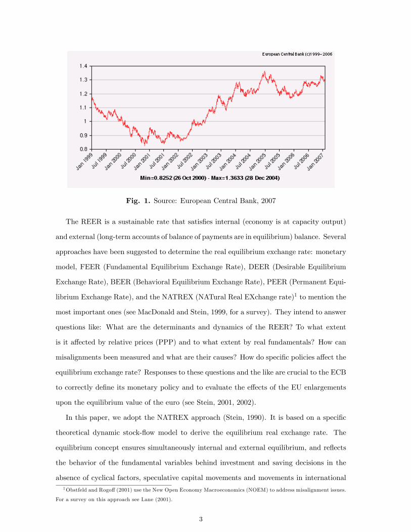
Fig. 1. Source: European Central Bank, 2007
The REER is a sustainable rate that satis�es internal (economy is at capacity output)
and external (long-term accounts of balance of payments are in equilibrium) balance. Several
approaches have been suggested to determine the real equilibrium exchange rate: monetary
model, FEER (Fundamental Equilibrium Exchange Rate), DEER (Desirable Equilibrium
Exchange Rate), BEER (Behavioral Equilibrium Exchange Rate), PEER (Permanent Equi-
librium Exchange Rate), and the NATREX (NATural Real EXchange rate)1 to mention the
most important ones (see MacDonald and Stein, 1999, for a survey). They intend to answer
questions like: What are the determinants and dynamics of the REER? To what extent
is it a¤ected by relative prices (PPP) and to what extent by real fundamentals? How can
misalignments been measured and what are their causes? How do speci�c policies a¤ect the
equilibrium exchange rate? Responses to these questions and the like are crucial to the ECB
to correctly de�ne its monetary policy and to evaluate the e¤ects of the EU enlargements
upon the equilibrium value of the euro (see Stein, 2001, 2002).
In this paper, we adopt the NATREX approach (Stein, 1990). It is based on a speci�c
theoretical dynamic stock-�ow model to derive the equilibrium real exchange rate. The
equilibrium concept ensures simultaneously internal and external equilibrium, and re�ects
the behavior of the fundamental variables behind investment and saving decisions in the
absence of cyclical factors, speculative capital movements and movements in international1Obstfeld and Rogo¤ (2001) use the New Open Economy Macroeconomics (NOEM) to address misalignment issues.
For a survey on this approach see Lane (2001).
3
reserves. Several notable studies have already adopted the NATREX approach to explain
the medium-long term dynamics of the real exchange rate in a number of industrial coun-
tries: USA (Stein, 1995, 1997), Australia (Lim and Stein, 1995), Germany (Stein and
Sauernheimer, 1996), France (Stein and Paladino, 1999), Italy (Gandolfo and Felettigh,
1998; Federici and Gandolfo, 2002), Belgium (Verrue and Colpaert, 1998), the Eurozone
(Detken and Marin, 2002; Duval, 2002), China (Holger et al., 2001), and Hungary (Karadi,
2003). However, in the previous literature, the NATREX approach has been applied to a
one-country framework where the �rest of the world� is treated as given. Yet, the recog-
nition of the interdependence of the world economy requires to extend the framework and
endogenize the �rest of the world�in a two-country context. This work is the �rst to build
a two-country NATREX model and apply it to the Eurozone and the US. The theoretical
model presented in this paper o¤ers the basis for empirical estimation that will be carried
out in future research.
The remainder of this paper is organized as follows. Section 2 brie�y introduces the
theory of NATREX. Section 3 reviews the main alternative approaches to the equilibrium
exchange rate provided by the literature and the previous empirical applications to the
euro/dollar. Section 4 presents our theoretical model, whereas Sections 5 and 6 respectively
illustrate the NATREX derivation and the qualitative analysis of the model.
2 NATREX approach
In this section we brie�y recall the theoretical framework of the NATREX approach: for a
complete treatment, the reader should consult Allen (1995) and Stein (1995, 2001, 2006).
Following Stein (2001), the NATREX is a moving equilibrium exchange rate responding
to continual changes in exogenous real fundamentals, and representing the trajectory of
the medium-to-long run equilibrium. Therefore it may be interpreted as a benchmark from
which misalignments of the actual real exchange rate are measured. Denoting the real
economic fundamentals by Z; foreign debt by F and domestic output by Y , the actual real
exchange rate (E) can be written as:
E = fE (Z) + E (F;Z)� E (Z)g+ [E � E (F;Z)]
4
where E (F;Z) is the NATREX. Whence, simplifying the terms within the curly brackets,
we have:
E = NATREX + deviations
The NATREX represents the intercyclical equilibrium real exchange rate that ensures
the balance of payments� equilibrium in the absence of cyclical factors, speculative capi-
tal movements, changes in monetary policy, and movements in international reserves. In
other words, the NATREX is the equilibrium real exchange rate that would prevail if the
above-mentioned factors could be removed and the GNP were at capacity. Since it is an
equilibrium concept, the NATREX should guarantee the attainment of both internal and
external equilibrium, the focus being on the long run. The long-run internal equilibrium is
achieved when the economy is at capacity output, that is when the rate of capacity utiliza-
tion is at its stationary mean: de�ationary and in�ationary pressures are excluded. The
long-run external equilibrium is achieved when the long-term accounts of the balance of
payments are in equilibrium. Short term (speculative) capital movements and movements
in o¢ cial reserves are bound to be short term transactions, since they are unsustainable
in the long run. In the long-run equilibrium they must average out at zero; hence, the
excess of national (private plus public) investment over national saving must be entirely
�nanced through international long term borrowing. Thus, unlike other models of REER,
the NATREX approach adds dynamics to the determination of the REER.
Under these conditions long term capital in�ows and excess national investment over
saving coincide, so that also the real market long run equilibrium condition and the long
term external equilibrium condition coincide. The framework of the approach lies on the
national income accounting equation:
S � I = CA; (1)
where CA is the balance of payments� current account, the private and public sectors
having been aggregated into a single one. Relation (1) is intended in real terms: the model
assumes neutrality of money and that monetary policy keeps in�ation at a level compatible
with internal equilibrium (at least in the long run). Therefore, the focus being on the real
part of the economy, there is no need to model the money market. Perfect international
5
capital mobility is assumed: the real interest rate is driven by the portfolio equilibrium
condition or real interest parity condition, possibly with a risk premium.
The system is assumed to be self-equilibrating (hence the adjective natural in the
acronym NATREX). Take for example an initial position of full equilibrium (S� I = CA =
0) and suppose an exogenous shock leads to a situation where S � I < 0. Given the per-
fect international capital mobility, the interest rate cannot play the role of the adjustment
variable; rather, the di¤erence between national investment and national saving originates
a corresponding in�ow of long-term capital. The RER appreciates accordingly, leading to a
deterioration in the current account. The capital in�ow also causes an increase in the stock
of foreign debt, which in turn determines a decrease in total consumption (household and
government) and hence an increase in saving, until equilibrium is restored. In conclusion,
the RER is the adjustment variable in equation (1).
The hypothesis of perfect foresight is rejected. Rather, rational agents that e¢ ciently
use all the available information will base their intertemporal decisions upon a sub-optimal
feedback control (SOFC) rule (Infante and Stein, 1973; Stein, 1995). Basically, SOFC starts
from the observation that the optimal solution derived from standard optimization tech-
niques in perfect-knowledge perfect-foresight models has the saddle-path stability property,
hence the slightest error in implementing the stable arm of the saddle will put the system on
a trajectory that will diverge from the optimal steady state. Actual optimizing agents know
that they do not possess the perfect knowledge required to implement the stable arm of the
saddle without error, hence it is rational for them to adopt SOFC, which is a closed loop
control that only requires current measurements of a variable, not perfect foresight, and
will put the economy on a trajectory which is asymptotic to the unknown perfect-foresight
stable arm of the saddle.
The consumption and investment functions are derived accordingly, through dynamic
programming techniques with feedback control. No di¤erence is made between the private
and the public decisional process. The model can be solved for its medium run and long run
(steady state) solutions. Any perturbation on the real fundamentals of the system pushes
the equilibrium RER on a new medium-to-long-run trajectory. Since cyclical, transitory
and speculative factors are considered noise, averaging out at zero in the long run, the
6
actual RER converges to the equilibrium trajectory. The PPP theory turns out to be only
a special case of the NATREX approach: �the issue is not whether or not the real exchange
rate is stationary over an arbitrary period, but whether it re�ects the [real] fundamentals.�
(Stein, 1995, p. 43).
3 Alternative approaches to the euro/dollar equilibrium ex-
change rate
3.1 Other than NATREX
Several ways of calculating equilibrium exchange rates have been suggested in the litera-
ture. While for a complete survey we refer the reader to MacDonald and Stein (1999), in
this subsection we only consider empirical works that have been applied to the euro/dollar2
(for a survey see Stein, 2001, and ECB, 2002. For further considerations on the alterna-
tive approaches to the euro/dollar see Williamson 2004). We can distinguish three broad
categories: monetary, statistical and structural approaches.
The monetary approach models the nominal exchange rate as the interaction between
the relative demand for and supply of two currencies. Accordingly the nominal exchange
rate, e.g., of the euro/dollar appreciates (depreciates) in the event of a relative decrease
(increase) in the money supply of, or a relative increase (decrease) in the money demand
for, euros. It follows that in addition to monetary aggregates and base money, further
determinants of the exchange rate are factors that in�uence the demand for money such
as income, interest rates and in�ation rate. Monetary models for the euro/dollar exchange
rate have been developed and estimated by Chinn and Alquist (2002) and van Aarle et al.
(2000).
The BEER (Behavioral Equilibrium Exchange Rate; Clark and MacDonald, 1999) be-
longs to the second group. Di¤erently from the structural approaches, the BEER relies on a
statistical concept of equilibrium. Its calculation involves the estimation of a reduced-form
equation that explains the behavior of the actual real exchange rate in terms of a set of
long-run (such as terms of trade, net foreign assets, relative government debt, and price2We remark that, due to the lack of long-span series for the actual euro/dollar exchange rate, most of these studies
use the synthetic euro.
7
indices) and medium-run (such as real interest rate di¤erential) economic fundamentals,
and a set of transitory factors a¤ecting the real exchange rate in the short run. A number
of empirical studies have applied this methodology to estimate the equilibrium exchange
rate of the euro/dollar: Gern et al. (2000), Clostermann and Shnatz (2000), and Lorenzen
and Thygesen (2000); and of the euro real e¤ective exchange rate: Koen et al. (2001), and
Maeso-Fernandez et al. (2001)3.
The measured BEER, generated from variables that are highly persistent and often non-
stationary, is likely to be a very persistent series as well. Adopting the Johansen cointegra-
tion method, the vector of cointegrated variables underlying the BEER can be decomposed
into permanent and transitory components (see Clark and MacDonald, 2004). The PEER
(Permanent Equilibrium Exchange Rate) is derived considering only the former ones. The
PEER has been estimated for the euro/dollar by Alberola et al. (1999) and Hansen and
Roeger (2000), and for the euro real e¤ective exchange rate by Alberola et al. (1999), and
Maeso-Fernandez et al. (2001).
Among the structural approaches to the real equilibrium exchange rate, the FEER (Fun-
damental Equilibrium Exchange Rate, Williamson, 1985, 1994) is the main alternative to
the NATREX (illustrated in Section (2)). In this approach the equilibrium exchange rate is
de�ned as the real exchange rate that is consistent with macroeconomic balance, which is
generally interpreted as when the economy is operating at full employment and low in�ation
(internal balance), and a current account that is sustainable, i.e. re�ects underlying net
capital �ows (external balance). The core of the FEER approach is the identity equating
the current account (CA) to the (negative of) the capital account (NFA). The attention of
the method is on the determinants of the current account, which is generally explained as a
function of home and foreign output or demand and the real e¤ective exchange rate. Given
the parameters of the current account, including in particular the sensitivity of current ac-
count �ows to the real exchange rate, the FEER is calculated using an exogenously given
estimate of sustainable net capital �ows. The main di¤erence between the FEER and the
NATREX lies on the fact that while the former is a medium-term concept where external3Bénassy-Quéré et al. (2006) adopt the BEER approach to derive consistent real e¤ective equilibrium exchange
rate for 15 countries of the G20.
8
and internal balance prevails, the latter explains the determinants of the evolution of the
real equilibrium exchange rate in the medium to the longer run, where the net foreign debt
is constant and the capital stock is at its steady state level. The FEER approach has been
adopted to estimate the real equilibrium exchange rate of the euro/dollar by Wren-Lewis
and Driver (1998), and Borowski and Couharde (2000).
Finally two further approaches to the equilibrium exchange rate are the DEER (Desirable
Equilibrium Exchange Rate) and the CHEER (Capital Enhanced Equilibrium Exchange
Rate). The former (see Bayoumi et al., 1994) is a variant of the FEER and assumes target
values for the macroeconomic objectives, such as targeted current account surplus for each
country. The latter (see MacDonald, 2000, 2006) exploits the cointegration properties of
the interest rate di¤erentials and the real exchange rate.
3.2 NATREX
At the best of our knowledge, there are only two applications of the NATREX approach
to the Eurozone, namely Detken et al. (2002)4 and Duval (2002), both considering the
exchange rate of the synthetic euro vis-à-vis the US dollar from early 1970 to 2000. Whereas
the former employ a multiple-equation structural model estimation, the latter implements
a reduced form single equation estimation as described in what follows.
Duval (2002) builds a dynamic model for the real equilibrium exchange rate of the
euro/dollar combining the NATREX and the BEER approaches. First, the long run REER
for tradable goods (eLTT denotes the variable in logarithmic terms) is modelled as a NA-
TREX. Accordingly, the author obtains the reduced-form equation of eLTT as a function of
the time preferences (ct) and technological progress (at):
eLT;iT = eLT;iT (at; ct) (2)
where i stands for either the Eurozone (EU) or the United States (US). Second, (2) is
combined with the real equilibrium exchange rate of the euro/dollar for the whole economy
(eLT ), that is:
eLT = eLTT + ���pUSNT � pUST
���pEUNT � pEUT
��(3)
4See also Detken and Marin-Martinez (2001).
9
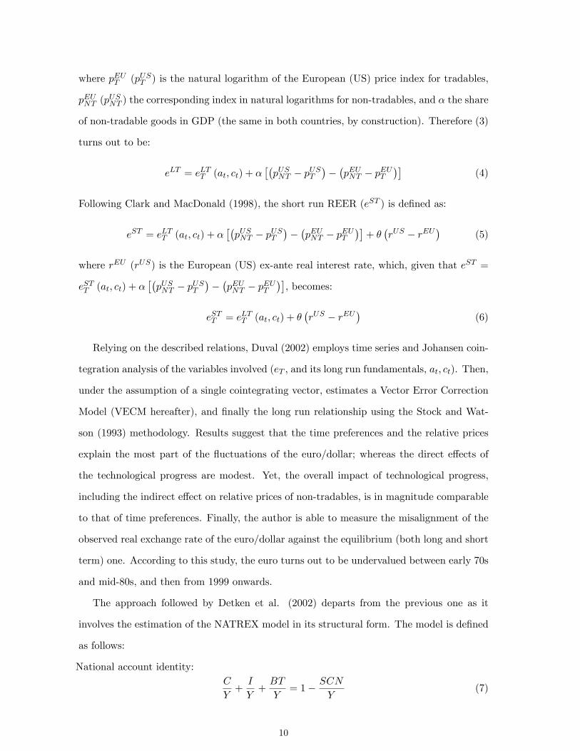
where pEUT (pUST ) is the natural logarithm of the European (US) price index for tradables,
pEUNT (pUSNT ) the corresponding index in natural logarithms for non-tradables, and � the share
of non-tradable goods in GDP (the same in both countries, by construction). Therefore (3)
turns out to be:
eLT = eLTT (at; ct) + ���pUSNT � pUST
���pEUNT � pEUT
��(4)
Following Clark and MacDonald (1998), the short run REER (eST ) is de�ned as:
eST = eLTT (at; ct) + ���pUSNT � pUST
���pEUNT � pEUT
��+ �
�rUS � rEU
�(5)
where rEU (rUS) is the European (US) ex-ante real interest rate, which, given that eST =
eSTT (at; ct) + ���pUSNT � pUST
���pEUNT � pEUT
��, becomes:
eSTT = eLTT (at; ct) + ��rUS � rEU
�(6)
Relying on the described relations, Duval (2002) employs time series and Johansen coin-
tegration analysis of the variables involved (eT ; and its long run fundamentals, at; ct). Then,
under the assumption of a single cointegrating vector, estimates a Vector Error Correction
Model (VECM hereafter), and �nally the long run relationship using the Stock and Wat-
son (1993) methodology. Results suggest that the time preferences and the relative prices
explain the most part of the �uctuations of the euro/dollar; whereas the direct e¤ects of
the technological progress are modest. Yet, the overall impact of technological progress,
including the indirect e¤ect on relative prices of non-tradables, is in magnitude comparable
to that of time preferences. Finally, the author is able to measure the misalignment of the
observed real exchange rate of the euro/dollar against the equilibrium (both long and short
term) one. According to this study, the euro turns out to be undervalued between early 70s
and mid-80s, and then from 1999 onwards.
The approach followed by Detken et al. (2002) departs from the previous one as it
involves the estimation of the NATREX model in its structural form. The model is de�ned
as follows:
National account identity:C
Y+I
Y+BT
Y= 1� SCN
Y(7)
10
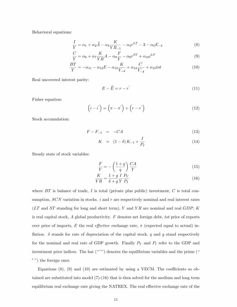
Behavioral equations:
I
Y= �1 + �2 bA� �3 K
Y R�1� �4rLT � 3� �5E�4 (8)
C
Y= �6 + �7
K
Y RA� �8
F
Y� �9rST + �10iLT (9)
BT
Y= ��11 � �12E � �13
K
Y�4+ �14
C0
Y0
�4+ �15tot (10)
Real uncovered interest parity:
E � bE = r � r0 (11)
Fisher equation: �i� i0
�=�� � �0
�+�r � r0
�(12)
Stock accumulation:
F � F�1 = �CA (13)
K = (1� �)K�1 +I
PI(14)
Steady state of stock variables:
F
Y= �
�1 + q
q
�CA
Y(15)
K
Y R=1 + g
� + g
I
Y
PYPI
(16)
where BT is balance of trade, I is total (private plus public) investment, C is total con-
sumption, SCN variation in stocks. i and r are respectively nominal and real interest rates
(LT and ST standing for long and short term), Y and Y R are nominal and real GDP ; K
is real capital stock, A global productivity. F denotes net foreign debt, tot price of exports
over price of imports, E the real e¤ective exchange rate, � (expected equal to actual) in-
�ation. � stands for rate of depreciation of the capital stock, q and g stand respectively
for the nominal and real rate of GDP growth. Finally PY and PI refer to the GDP and
investment price indices. The hat (�b�) denotes the equilibrium variables and the prime (�
0 �) the foreign ones.
Equations (8), (9) and (10) are estimated by using a VECM. The coe¢ cients so ob-
tained are substituted into model (7)-(16) that is then solved for the medium and long term
equilibrium real exchange rate giving the NATREX. The real e¤ective exchange rate of the
11
synthetic euro is then compared with the benchmark generated by the model simulations
to measure the misalignments, if any. It turns out that the synthetic euro was overvalued
from the second half of the �70s until the early �80s; periods of over- and under-evaluations
alternate thereafter until 1997 when it fell and stayed below the equilibrium value (more
remarkably starting from 1999 onwards) for the remaining part of the period considered.
Also, Detken et al. (2002) emphasize the main driving forces of the dynamics of the equi-
librium exchange rate for the euro resulting from their work, and namely the productivity
growth and the terms of trade.
4 Two-country NATREX model
We consider two large economies, the Eurozone (EU) and the United States (US), which
are modelled symmetrically. The model is de�ned by dynamic equations for fundamental
variables in each country plus the national account identities. The equations specify the
dynamics for, respectively: net social investment, internal social consumption, trade balance
(goods and services), interest rate, technology and capital stock. As already observed in
Section 2, variables adjust with a certain lag to their desired (partial equilibrium) level,
according to the dynamic disequilibrium modelling approach in continuous time. In what
follows variables are real, �D�denotes the operator d=dt, the hat �b�stands for �desired�,and all coe¢ cients are written in such a way that they are supposed to be positive unless
otherwise stated. Furthermore, the exchange rate (E) for the euro/dollar is de�ned as the
number of US dollars per one euro; it follows that an increase in E means an appreciation of
the euro (the euro gets stronger) vis-à-vis the US dollar. Finally, we notice that, while the
rest of the world is not explicitly modelled in the theoretical framework, in the empirical
estimation it will be captured by exogenous correction factors.
4.1 Investment
Saving and investment decisions are made independently by individual agents. This is
equivalent to saying that families choose saving and consumption, while �rms decide over
investment and production. Total investment (I) is given by the sum of private and public
investment. It adjusts to its partial equilibrium level with a mean time lag (1=�1) due to
12
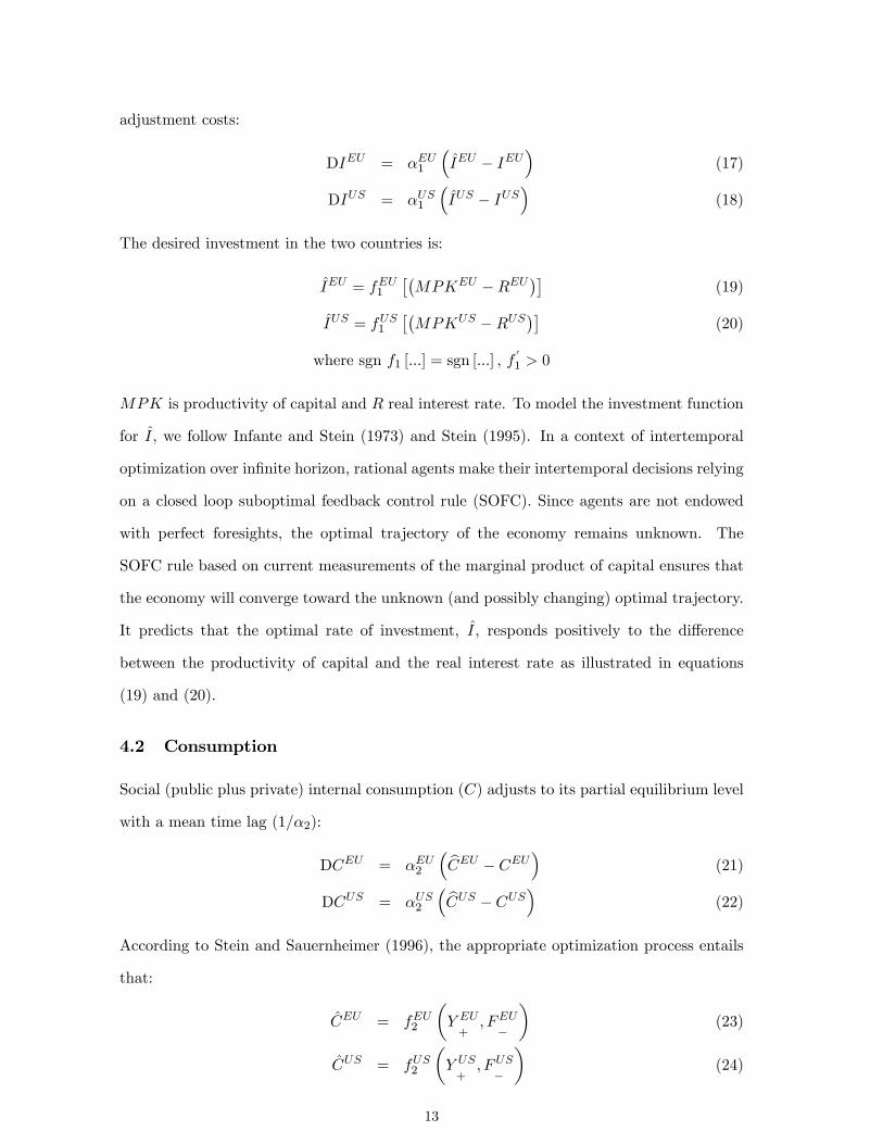
adjustment costs:
DIEU = �EU1
�IEU � IEU
�(17)
DIUS = �US1
�IUS � IUS
�(18)
The desired investment in the two countries is:
IEU = fEU1��MPKEU �REU
��(19)
IUS = fUS1��MPKUS �RUS
��(20)
where sgn f1 [:::] = sgn [:::] , f0
1 > 0
MPK is productivity of capital and R real interest rate. To model the investment function
for I, we follow Infante and Stein (1973) and Stein (1995). In a context of intertemporal
optimization over in�nite horizon, rational agents make their intertemporal decisions relying
on a closed loop suboptimal feedback control rule (SOFC). Since agents are not endowed
with perfect foresights, the optimal trajectory of the economy remains unknown. The
SOFC rule based on current measurements of the marginal product of capital ensures that
the economy will converge toward the unknown (and possibly changing) optimal trajectory.
It predicts that the optimal rate of investment, I, responds positively to the di¤erence
between the productivity of capital and the real interest rate as illustrated in equations
(19) and (20).
4.2 Consumption
Social (public plus private) internal consumption (C) adjusts to its partial equilibrium level
with a mean time lag (1=�2):
DCEU = �EU2
� bCEU � CEU� (21)
DCUS = �US2
� bCUS � CUS� (22)
According to Stein and Sauernheimer (1996), the appropriate optimization process entails
that:
CEU = fEU2
�Y EU+
; FEU�
�(23)
CUS = fUS2
�Y US+; FUS
�
�(24)
13
where Y denotes domestic output and F net foreign debt. The desired consumption function
is derived as follows. Private and public agents optimize their utility under an intertemporal
budget constraint. According to standard optimization theory, consumption is proportional
to current capacity output. When foreign debt grows above the level considered sustainable,
the government employes a restrictive �scal policy by decreasing current expenditure. This
gives that partial optimal consumption is a positive function of domestic output and a
negative function of foreign debt.
4.3 Trade balance
According to the NATREX theory, the partial adjustment process also holds for the balance
of trade (BT ):
DBTEU = �EU3
�dBTEU �BTEU� (25)
DBTUS = �US3
�dBTUS �BTUS� (26)
where BT = XGS �MGS, XGS denotes exports and MGS imports. The partial equilib-
rium values are:
dBTEU = fEU3
�Y US+; Y EU
�; E�
�(27)
dBTUS = fUS3
�Y EU+
; Y US�; E+
�(28)
and are obtained considering that, according to the standard assumptions in international
economics, real exports are a¤ected positively by the other country�s output, whereas im-
ports respond positively to the home country�s real output. Furthermore, given our de�-
nition for the euro/dollar exchange rate (number of US dollars per one euro), an increase
in E leads to an appreciation of the euro vis-à-vis the US dollar and, thus, to a decrease
(increase) of the EU (US) export and an increase (decrease) of the EU (US) imports. It fol-
lows that the partial �rst derivatives have the sign shown below the corresponding variables
in equations (27) and (28).
In a world made up of two countries (the Eurozone and the US), the following condition
must hold:
BTEU +1
EBTUS = 0 (29)
14
Given (29), one between (25) and (26) is redundant. Nonetheless, in view of the empirical
estimation of the model, we maintain both equations to also consider the rest of the world
e¤ect.
4.4 Real interest rates
The dynamic equations for the real interest rate (R) respectively in the Eurozone and in
the United States are given by5:
DREU = �EU4
� bREU �REU� (30)
DRUS = �US4
� bRUS �RUS� (31)
where:
bREU = RUS + �EU (32)
bRUS = REU + �US (33)
and � is the risk premium.
The real interest rate parity (RIP) theory states that if investors make their decisions in
real terms, then portfolio equilibrium in an open economy entails equality between expected
rates of return in real terms, possibly admitting a divergence corresponding to the risk
premium. In this model, investors face a long time horizon, deal with both direct and
portfolio investment, and trade domestic as well as foreign assets. Agents are rational
in the sense that they exploit all available information. Hence, investors keep trading,
and let interest di¤erentials adjust, until they become indi¤erent between domestic and
foreign assets, i.e. the RIP condition with risk premium holds ((32) and (33) respectively
for the Eurozone and the US). This condition, however, is not valid instantaneously, but
rather is achieved with a certain time lag (1=�4), due to market imperfections and to the
corresponding sluggishness in the re-equilibrating process, as described by (30) and (31).
Eaton and Gersovitz (1981) establish that, because of the moral hazard associated with
sovereign risk, the risk premium of international lending varies positively with the stock
of debt held by the given country. Moreover, Sachs (1984), Sachs and Cohen (1982), and
Cooper and Sachs (1985) suggest that the cost of servicing the debt may be curbed by5For the long run characteristics of the system composed of (30) and (31) see the mathematical appendix A.
15
means of growth-oriented policies and policies that enhance the country�s foreign exchange
earning capacity. It follows that the risk premiums may be expressed as a positive function
of the ratio between foreign debt and domestic output (van der Ploeg, 1996; Bhandari,
Hague, and Turnovsky, 1990), that is:
�EU = fEU4
�FEU=Y EU
+
�(34)
�US = fEU4
�FUS=Y US
+
�(35)
In the long run, two further conditions must hold. Indeed in a two-large economy world, a
situation where one country is continuously characterized by a positive, while the other by
a negative stock of foreign debt is not sustainable in the long run. Therefore, the long run
equilibrium requires that:
FEU = FUS = 0: (36)
Given equations (34) and (35), it also follows that:
�EU = �US = 0 (37)
4.5 Output
In the two economies, output adjusts with a lag (1=�5) to the excess demand:
DY EU = �EU5�Y EUD � Y EUS
�(38)
DY US = �US5�Y USD � Y USS
�(39)
where YD and YS are respectively aggregate demand and aggregate supply, and by national
account identity it turns out that YD = C + I + (XGS �MGS) :
In this paper we follow Federici and Gandolfo (2002) and introduce endogenous growth.
The production function is modelled in an �AK�fashion6, that is potential output, respec-
tively in the Eurozone and the United States, and is given by:
Y EUS = AEUKEU (40)
Y USS = AUSKUS (41)6For obvious reasons this function has come to be known in the recent literature as the �AK� production function
(Barro and Sala-i-Martin, 1995), but its use in growth theory has a long tradition: e.g. Harrod (1939) and Domar
(1946); Klump and Streissler (2000) show that the von Neumann production function can be reduced to the AK
type. More sophisticated forms (including other factors of production) could be considered, but on the basis of the
parsimony principle we decided to start with the simplest possible form.
16
where A is a positive constant which re�ects the technological level.
We generalize this approach by assuming that bA is function of the stock of accumulatedknowledge, , which has a positive but decreasing e¤ect. In addition, A () has an upper
limit �A, since it is implausible to think that the productivity of capital can go to in�nity.
Therefore:
bAEU = AEU (EU ) (42)
bAUS = AUS(US) (43)
with A0 > 0; A00 < 0; A � A
where may be in turn expressed as a function of the accumulated R&D expenditure
(IR&D):
EU = EUZ t
�1IEUR&D (s) ds or _ = EUIEUR&D (44)
US = USZ t
�1IUSR&D (s) ds or _ = USIUSR&D (45)
We assume that A adjusts with a lag (1=�6) to its partial equilibrium level, hence the
corresponding dynamic equations in the two economies are described by:
D lnAEU = �EU6 ln
bAEUAEU
!(46)
D lnAUS = �US6 ln
bAUSAUS
!(47)
Total investment (I) is divided between investment in �xed capital (IK) and investment in
R&D (IR&D):
IEU = IEUK + IEUR&D (48)
IUS = IUSK + IUSR&D (49)
R&D investment enhances the marginal productivity of capital (by increasing the stock of
accumulated knowledge) but with a lag ( ). The lag is crucial: more investment in R&D
means less increase in the capital stock and hence smaller growth immediately; it also means
higher productivity and thus higher growth later.
We need now to determine the optimal allocation of I between IK and IR&D. Given that
investment is private+public, we can think of the choice being determined by a maximizing
17
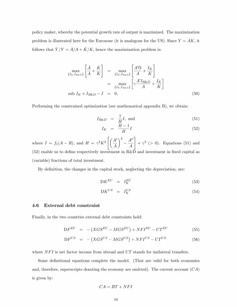
policy maker, whereby the potential growth rate of output is maximized. The maximization
problem is illustrated here for the Eurozone (it is analogous for the US). Since Y = AK, it
follows that _Y =Y = _A=A+ _K=K; hence the maximization problem is:
maxfIK ;IR&Dg
"_A
A+_K
K
#= max
fIK ;IR&Dg
"A0 _
A+IKK
#
= maxfIK ;IR&Dg
� A0IR&DA
+IKK
�sub IK + IR&D � I = 0; (50)
Performing the constrained optimization (see mathematical appendix B), we obtain:
IR&D =1
HI; and (51)
IK =H � 1H
I (52)
where I = f1(A � R), and H = 2K2
"�A0
A
�2� A00
A
#+ 2 (> 0). Equations (51) and
(52) enable us to de�ne respectively investment in R&D and investment in �xed capital as
(variable) fractions of total investment.
By de�nition, the changes in the capital stock, neglecting the depreciation, are:
DKEU = IEUK (53)
DKUS = IUSK (54)
4.6 External debt constraint
Finally, in the two countries external debt constraints hold:
DFEU = ��XGSEU �MGSEU
�+NFIEU � UTEU (55)
DFUS = ��XGSUS �MGSUS
�+NFIUS � UTUS (56)
where NFI is net factor income from abroad and UT stands for unilateral transfers.
Some de�nitional equations complete the model. (That are valid for both economies
and, therefore, superscripts denoting the economy are omitted). The current account (CA)
is given by:
CA = BT +NFI
18
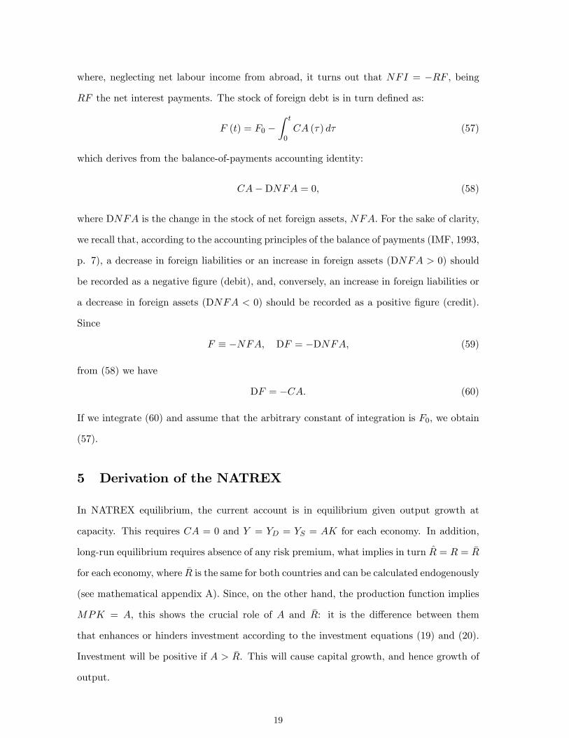
where, neglecting net labour income from abroad, it turns out that NFI = �RF , being
RF the net interest payments. The stock of foreign debt is in turn de�ned as:
F (t) = F0 �Z t
0CA (�) d� (57)
which derives from the balance-of-payments accounting identity:
CA�DNFA = 0; (58)
where DNFA is the change in the stock of net foreign assets, NFA: For the sake of clarity,
we recall that, according to the accounting principles of the balance of payments (IMF, 1993,
p. 7), a decrease in foreign liabilities or an increase in foreign assets (DNFA > 0) should
be recorded as a negative �gure (debit), and, conversely, an increase in foreign liabilities or
a decrease in foreign assets (DNFA < 0) should be recorded as a positive �gure (credit).
Since
F � �NFA; DF = �DNFA; (59)
from (58) we have
DF = �CA: (60)
If we integrate (60) and assume that the arbitrary constant of integration is F0, we obtain
(57).
5 Derivation of the NATREX
In NATREX equilibrium, the current account is in equilibrium given output growth at
capacity. This requires CA = 0 and Y = YD = YS = AK for each economy. In addition,
long-run equilibrium requires absence of any risk premium, what implies in turn R = R = �R
for each economy, where �R is the same for both countries and can be calculated endogenously
(see mathematical appendix A). Since, on the other hand, the production function implies
MPK = A, this shows the crucial role of A and �R: it is the di¤erence between them
that enhances or hinders investment according to the investment equations (19) and (20).
Investment will be positive if A > �R. This will cause capital growth, and hence growth of
output.
19
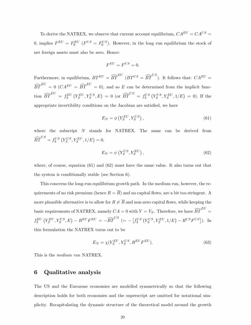
To derive the NATREX, we observe that current account equilibrium, CAEU = CAUS =
0, implies FEU = FEU0 (FUS = FUS0 ). However, in the long run equilibrium the stock of
net foreign assets must also be zero. Hence:
FEU = FUS = 0:
Furthermore, in equilibrium, BTEU =dBTEU (BTUS =dBTUS). It follows that: CAEU =dBTEU = 0 (CAEU = dBTEU = 0), and so E can be determined from the implicit func-
tion dBTEU = fEU3�Y EUS ; Y USS ; E
�= 0 (or dBTUS = fUS3
�Y USS ; Y EUS ; 1=E
�= 0): If the
appropriate invertibility conditions on the Jacobian are satis�ed, we have
EN = ��Y EUS ; Y USS
�; (61)
where the subscript N stands for NATREX. The same can be derived fromdBTUS = fUS3�Y USS ; Y EUS ; 1=E
�= 0,
EN = �Y USS ; Y EUS
�; (62)
where, of course, equation (61) and (62) must have the same value. It also turns out that
the system is conditionally stable (see Section 6).
This concerns the long-run equilibrium growth path. In the medium run, however, the re-
quirements of no risk premium (hence R = R) and no capital �ows, are a bit too stringent. A
more plausible alternative is to allow for R 6= R and non-zero capital �ows, while keeping the
basic requirements of NATREX, namely CA = 0 with Y = YS . Therefore, we havedBTEU =fEU3
�Y EUS ; Y USS ; E
�� REUFEU = �dBTUS (= �
�fUS3
�Y USS ; Y EUS ; 1=E
��RUSFUS
�). In
this formulation the NATREX turns out to be
EN = �(Y EUS ; Y USS ; REUFEU ): (63)
This is the medium run NATREX.
6 Qualitative analysis
The US and the Eurozone economies are modelled symmetrically so that the following
description holds for both economies and the superscript are omitted for notational sim-
plicity. Recapitulating the dynamic structure of the theoretical model around the growth
20
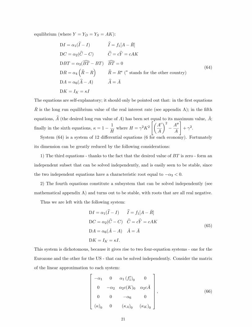
equilibrium (where Y = YD = YS = AK):
DI = �1(bI � I) bI = f1[A� �R]
DC = �2( bC � C) bC = cbY = cAK
DBT = �3(dBT �BT ) dBT = 0DR = �4
� bR�R� bR = R� (� stands for the other country)
DA = �6( bA�A) bA = �A
DK = IK = �I
(64)
The equations are self-explanatory; it should only be pointed out that: in the �rst equations
�R is the long run equilibrium value of the real interest rate (see appendix A); in the �fth
equations, bA (the desired long run value of A) has been set equal to its maximum value, �A;
�nally in the sixth equations, � = 1� 1
Hwhere H = 2K2
"�A0
A
�2� A00
A
#+ 2.
System (64) is a system of 12 di¤erential equations (6 for each economy). Fortunately
its dimension can be greatly reduced by the following considerations:
1) The third equations - thanks to the fact that the desired value of BT is zero - form an
independent subset that can be solved independently, and is easily seen to be stable, since
the two independent equations have a characteristic root equal to ��3 < 0:
2) The fourth equations constitute a subsystem that can be solved independently (see
mathematical appendix A) and turns out to be stable, with roots that are all real negative.
Thus we are left with the following system:
DI = �1(bI � I) bI = f1[A� �R]
DC = �2( bC � C) bC = cbY = cAK
DA = �6(A�A) A = �A
DK = IK = �I:
(65)
This system is dichotomous, because it gives rise to two four-equation systems - one for the
Eurozone and the other for the US - that can be solved independently. Consider the matrix
of the linear approximation to each system:266666664
��1 0 �1 (f01)0 0
0 ��2 �2c(K)0 �2c �A
0 0 ��6 0
(�)0 0 (�A)0 (�K)0
377777775; (66)
21
where �A =1
H2
@H
@A; �K =
1
H2
@H
@Kand (:::)0 denotes that the variable is evaluated at the
equilibrium point. Furthermore, it can be checked7 that@H
@A< 0;
@H
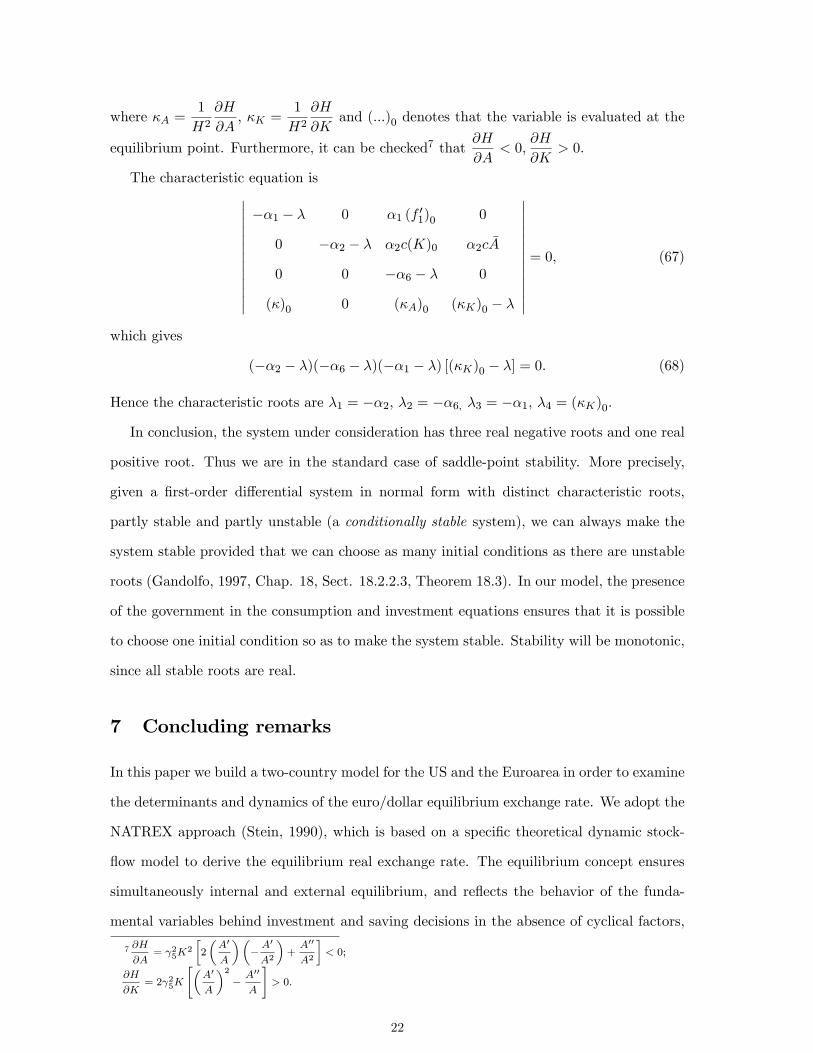
@K> 0:
The characteristic equation is�������������
��1 � � 0 �1 (f01)0 0
0 ��2 � � �2c(K)0 �2c �A
0 0 ��6 � � 0
(�)0 0 (�A)0 (�K)0 � �
�������������= 0; (67)
which gives
(��2 � �)(��6 � �)(��1 � �) [(�K)0 � �] = 0: (68)
Hence the characteristic roots are �1 = ��2; �2 = ��6; �3 = ��1; �4 = (�K)0.
In conclusion, the system under consideration has three real negative roots and one real
positive root. Thus we are in the standard case of saddle-point stability. More precisely,
given a �rst-order di¤erential system in normal form with distinct characteristic roots,
partly stable and partly unstable (a conditionally stable system), we can always make the
system stable provided that we can choose as many initial conditions as there are unstable
roots (Gandolfo, 1997, Chap. 18, Sect. 18.2.2.3, Theorem 18.3). In our model, the presence
of the government in the consumption and investment equations ensures that it is possible
to choose one initial condition so as to make the system stable. Stability will be monotonic,
since all stable roots are real.
7 Concluding remarks
In this paper we build a two-country model for the US and the Euroarea in order to examine
the determinants and dynamics of the euro/dollar equilibrium exchange rate. We adopt the
NATREX approach (Stein, 1990), which is based on a speci�c theoretical dynamic stock-
�ow model to derive the equilibrium real exchange rate. The equilibrium concept ensures
simultaneously internal and external equilibrium, and re�ects the behavior of the funda-
mental variables behind investment and saving decisions in the absence of cyclical factors,
7 @H
@A= 25K
2
�2
�A0
A
��� A
0
A2
�+A00
A2
�< 0;
@H
@K= 2 25K
"�A0
A
�2� A00
A
#> 0:
22
speculative capital movements and movements in international reserves. This approach
has already been applied to explain the medium-long term dynamics of the real exchange
rate in a number of industrial countries. However, the previous literature has relied on a
one-country framework where the �rest of the world�is treated as given. This work is the
�rst to fully specify the two economies and allow for their interaction. The model presents
a saddle point stability. Hence, once the initial condition is chosen, the system turns out
conditionally stable. Since the government takes part in the consumption and investment
decisions, the choice of the appropriate initial condition is always guaranteed. Our theoret-
ical model o¤ers the basis for empirical estimation of the euro/dollar equilibrium exchange
rate that will be carried out in future research.
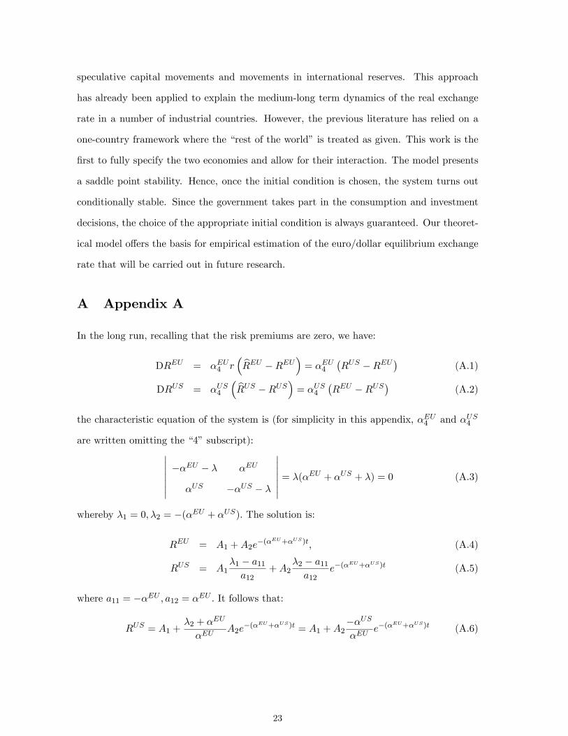
A Appendix A
In the long run, recalling that the risk premiums are zero, we have:
DREU = �EU4 r� bREU �REU� = �EU4
�RUS �REU
�(A.1)
DRUS = �US4
� bRUS �RUS� = �US4�REU �RUS
�(A.2)
the characteristic equation of the system is (for simplicity in this appendix, �EU4 and �US4
are written omitting the �4�subscript):���������EU � � �EU
�US ��US � �
������� = �(�EU + �US + �) = 0 (A.3)
whereby �1 = 0; �2 = �(�EU + �US): The solution is:
REU = A1 +A2e�(�EU+�US)t; (A.4)
RUS = A1�1 � a11a12
+A2�2 � a11a12
e�(�EU+�US)t (A.5)
where a11 = ��EU ; a12 = �EU : It follows that:
RUS = A1 +�2 + �
EU
�EUA2e
�(�EU+�US)t = A1 +A2��US�EU
e�(�EU+�US)t (A.6)
23
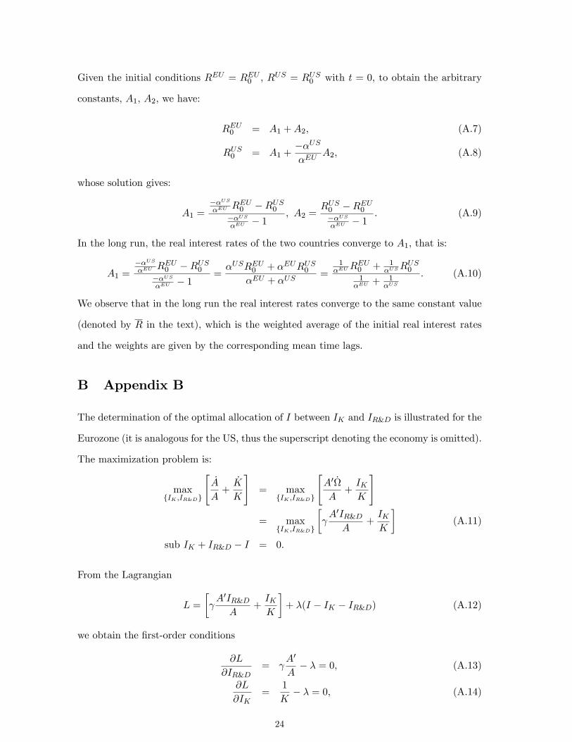
Given the initial conditions REU = REU0 ; RUS = RUS0 with t = 0, to obtain the arbitrary
constants, A1, A2, we have:
REU0 = A1 +A2; (A.7)
RUS0 = A1 +��US�EU
A2; (A.8)
whose solution gives:
A1 =��US�EU REU0 �RUS0
��US�EU � 1
; A2 =RUS0 �REU0��US�EU � 1
: (A.9)
In the long run, the real interest rates of the two countries converge to A1, that is:
A1 =��US�EU REU0 �RUS0
��US�EU � 1
=�USREU0 + �EURUS0
�EU + �US=
1�EUR
EU0 + 1
�USRUS0
1�EU +
1�US
: (A.10)
We observe that in the long run the real interest rates converge to the same constant value
(denoted by R in the text), which is the weighted average of the initial real interest rates
and the weights are given by the corresponding mean time lags.
B Appendix B
The determination of the optimal allocation of I between IK and IR&D is illustrated for the
Eurozone (it is analogous for the US, thus the superscript denoting the economy is omitted).
The maximization problem is:
maxfIK ;IR&Dg
"_A
A+_K
K
#= max
fIK ;IR&Dg
"A0 _
A+IKK
#
= maxfIK ;IR&Dg
� A0IR&DA
+IKK
�(A.11)
sub IK + IR&D � I = 0:
From the Lagrangian
L =
� A0IR&DA
+IKK
�+ �(I � IK � IR&D) (A.12)
we obtain the �rst-order conditions
@L
@IR&D=
A0
A� � = 0; (A.13)
@L
@IK=
1
K� � = 0; (A.14)
24
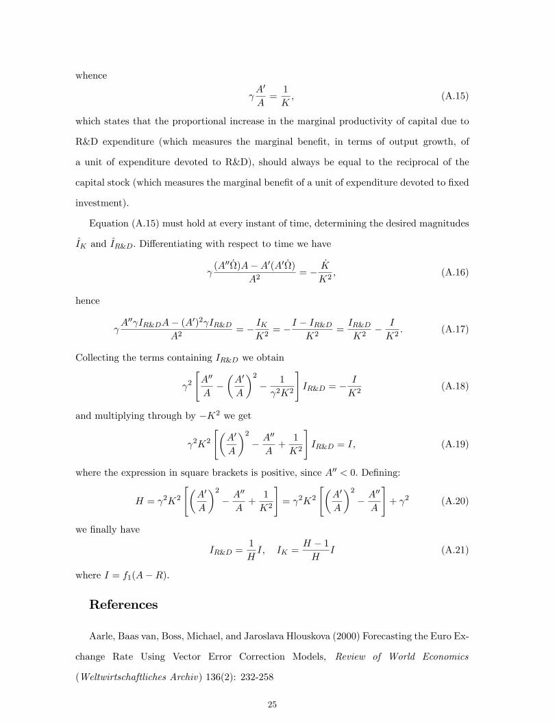
whence
A0
A=1
K; (A.15)
which states that the proportional increase in the marginal productivity of capital due to
R&D expenditure (which measures the marginal bene�t, in terms of output growth, of
a unit of expenditure devoted to R&D), should always be equal to the reciprocal of the
capital stock (which measures the marginal bene�t of a unit of expenditure devoted to �xed
investment).
Equation (A.15) must hold at every instant of time, determining the desired magnitudes
IK and IR&D: Di¤erentiating with respect to time we have
(A00 _)A�A0(A0 _)
A2= �
_K
K2; (A.16)
hence
A00 IR&DA� (A0)2 IR&D
A2= � IK
K2= �I � IR&D
K2=IR&DK2
� I
K2: (A.17)
Collecting the terms containing IR&D we obtain
2
"A00
A��A0
A
�2� 1
2K2
#IR&D = �
I
K2(A.18)
and multiplying through by �K2 we get
2K2
"�A0
A
�2� A00
A+
1
K2
#IR&D = I; (A.19)
where the expression in square brackets is positive, since A00 < 0: De�ning:
H = 2K2
"�A0
A
�2� A00
A+
1
K2
#= 2K2
"�A0
A
�2� A00
A
#+ 2 (A.20)
we �nally have
IR&D =1
HI; IK =
H � 1H
I (A.21)
where I = f1(A�R):
References
Aarle, Baas van, Boss, Michael, and Jaroslava Hlouskova (2000) Forecasting the Euro Ex-
change Rate Using Vector Error Correction Models, Review of World Economics
(Weltwirtschaftliches Archiv) 136(2): 232-258
25
Alberola, Enrique, Cervero, Susana G., Lopez, Humberto, and Angel Ubide (1999)
Global Equilibrium Exchange Rates: Euro, Dollar, �ins,��outs,�and Other Major Curren-
cies in a Panel Cointegration Framework, IMF Working Paper 175
Allen, Polly Reynolds (1995) The Economic and Policy Implications of the NATREX
Approach, in Jerome L. Stein, Polly Reynolds Allen et al., 1995, Fundamental Determinants
of Exchange Rates, Oxford University Press.
Alquist, Ron, and Menzie D. Chinn (2002) Productivity and the Euro-Dollar Exchange
Rate Puzzle, NBER Working Paper 8824
Bayoumi, Tamim, Peter Clark, Steve Symansky, and Mark Taylor (1994) The Robustness
of Equilibrium Exchange Rate Calculations to Alternative Assumptions and Methodologies,
in John Williamson (ed), Estimating Equilibrium Exchange Rates, Washington: Institute
for International Economics
Bailey, Andrew John, and Stephen Millard (2001) Capital Flows and Exchange Rates,
Bank of England Quarterly Bulletin (Autumn): 310-318
Bénassy-Quéré, Agnès, Lahrèche-Révil, Amina, and Valérie Mignon (2006) World Con-
sistent Equilibrium Exchange Rates, CEPII Working Paper 20
Bhandari, Jagdeep S., Haque, Nadeem Ul, and Stephen J. Turnovsky (1989) Growth,
External Debt, and Sovereign Risk in a Small Open Economy, IMF Sta¤ Papers 37: 388-417
Chinn, Menzie D., and Ron Alquist (2002) Tracking the Progress of Euro, International
Finance 3(3): 357-373
Clark, Peter, and Ronald MacDonald (1999) Exchange Rate and Economic Fundamen-
tals, in Ronald MacDonald and Jerome L. Stein (eds), Equilibrium Exchange Rates, Kluwer
Academic Publishers (Dordrecht): 285-322
Clark, Peter, and Ronald MacDonald (2004) Filtering the BEER: a Permanent and
Transitory Decomposition, Global Finance Journal 15: 29-56
Clostermann, Jörg and Bernd Schnatz (2000) The Determinants of the Euro-Dollar
Exchange Rate: Synthetic Fundamentals and a Non-Existing Currency, Konjunkturpoli-
tik/Applied Economics Quarterly 46 (3): 274-302
Cohen, Daniel, and Olivier Loisel (2001) WhyWas the EuroWeak? Markets and Policies,
European Economic Review 45: 988-994
26
Cooper, Richard N. and Je¤rey D. Sachs (1984) Borrowing Abroad: The Debtor�s Per-
spective, NBER Working Paper 1427
De Grauwe, Paul (2000) Exchange Rates in Search of Fundamentals: The Case of the
Euro-Dollar Rate, International Finance 3(3): 329-356
De Grauwe, Paul, and Marianna Grimaldi (2005) The Exchange Rate and its Funda-
mentals in a Complex World, Review of International Economics 13 (3): 549-575
Detken, Carsten and Carmen Marin-Martinez (2001) The E¤ective Euro Equilibrium
Exchange Rate Since the 1970�s: A Structural NATREX Estimation, European Central
Bank, Working Paper available at webdeptos.uma.es
Detken, Carsten, Dieppe, Alistair, Henry Jerome, Smets Frank, and Carmen Marin-
Martinez (2002) Determinants of the E¤ective Real Exchange Rate of the Synthetic Euro:
Alternative Methodological Approaches, Australian Economic Papers 41(4): 405-436
Domar, Evsey D. (1946) Capital Expansion, Rate of Growth and Employment, Econo-
metrica 14(2): 137-47
Duval, Romain (2002) What Do We Know about Long Run Equilibrium Real Exchange
Rates? PPPs vs Macroeconomic Approaches, Australian Economic Papers 41(4): 382-403
European Central Bank (2002) Economic Fundamentals and the Exchange Rate of the
Euro, ECB Monthly Bulletin (January): 41-53
European Central Bank (2007) Euro Foreign Exchange Reference Rates at
http://www.ecb.int/stats/exchange/eurofxref/html/eurofxref-graph-usd.en.html
Federici, Daniela, and Giancarlo Gandolfo (2002) Endogenous Growth in an Open Econ-
omy and the Real Exchange Rate, Australian Economic Papers 41(4): 499-518
Gandolfo, Giancarlo (1997) Economic Dynamics, Springer-Verlag, Berlin
Gern, Klaus-Jürgen, Kamps, Christophe, Meier, Carsten-Patrick, and Joachim Scheide
(2000) Euroland: Peak of the Upswing�Little Evidence of a New Economy, Kiel Discussion
Papers 369
Hansen, Jan, and Roeger, Werner (2000) Estimation of Real Equilibrium Exchange
Rates, European Commission Economic Papers (Brussels) 144
Harrod, Roy F. (1939) An Essay in Dynamic Theory, Economic Journal 49(193): 14-33
Holger, van Eden, Liu, Bin, Gerbert, Romyn, and Xiaoguang G. Yang (2001) NATREX
27
and Determinants of the Real Exchange Rate of RMB, Journal of Systems Science & Com-
plexity 14 (4): 356-372
IMF - International Monetary Fund (1993) Balance of Payments Manual, 5th edition
Infante, Ettore F., and Jerome L. Stein (1973) Optimal Growth with Robust Feedback
Control, Review of Economic Studies 15: 47-60
Karadi, Peter (2003), Structural and Single Equation Estimation of the NATREX Equi-
librium Real Exchange Rate, Central Bank of Hungary, Working Paper
Klump, Rainer, and Harald Preissler (2000) CES Production Functions and Economic
Growth, Scandinavian Journal of Economics 102(1): 41-56.
Koen, Vincent, Boone, Laurence, de Serres, Alain, and Nicola Fuchs (2001) Tracking the
Euro, OECD Economics Department Working Paper 24
Lane, Philip R. (2001) The New Open Economy Macroeconomics: A Survey, Journal of
International Economics 54: 235-266
Lim, Guay C., and J.L. Stein (1995) The Dynamics of the Real Exchange Rate and
Current Account in a Small Open Economy: Australia, in J.L. Stein, P.R. Allen, et al
(eds.) Fundamental Determinants of the Exchange Rates, Oxford University Press, Oxford
Lorenzen, Hans Peter, and Niels Thygesen (2000) The Relation between the Euro and
the Dollar, paper presented at the EPRU Conference, Copenhangen
MacDonald, Ronald (2000) Concepts to Calculate Equilibrium Exchange Rates: An
Overview, Deutsche Bundesbank Discussion Paper 3
MacDonald, Ronald (2005) Exchange Rate Economics: Theories and Evidence, Taylor
and Francis, forthcoming
MacDonald, Ronald, and Jerome L. Stein (1999) Equilibrium Exchange Rates, Kluwer
Academic Publishers, Dordrecht
Maeso-Fernandez, Francisco, Chiara Osbat and Bernd Schnatz (2002) Determinants of
the Euro Real E¤ective Exchange Rate: a BEER/PEER Approach, Australian Economic
Papers 41(4): 437-461
Obstfeld, Maurice, and Kenneth Rogo¤ (2001) Perspectives on OECD Economic Inte-
gration: Implications for US Current Account Adjustment, paper presented at the Jackson
Hole Conference, Federal Reserve Bank of Kansas
28
Ploeg, van der Frederik (1996) Budgetary Policies, Foreign Indebtedness, the Stock Mar-
ket, and Economic Growth, Oxford Economic Papers 48: 382-396
Sachs, Je¤rey D. (1984) Theoretical issues in International Borrowing, Princeton Studies
in International Finance 54
Sachs, Je¤rey D., and Daniel Cohen (1982) LDC Borrowing with Default Risk, NBER
Working Paper 925
Shams, Rasul (2005) Exchange Rate 1999-2004-Dollar and Euro as International Cur-
rencies, Hamburgisches Welt-Wirtschafts-Archiv (HWWA) Discussion Paper 321
Sinn, Hans-Werner, and Frank Westermann (2001) Why Has the Euro Been Falling?,
CESifo Working Paper 493
Stein, Jerome L. (1990) The Real Exchange Rate, Journal of Banking and Finance 14:
1045-1078
Stein, Jerome L. (1995) The Fundamental Determinants of the Real Exchange Rate of
the US Dollar Relative to the Other G-7 Countries, IMF Working Paper 95/81
Stein, Jerome L. (2001) The Equilibrium Value of the Euro/$ US Exchange Rate: an
Evaluation of Research, CESifo Working Papers 525
Stein, Jerome L. (2002) Enlargement and the Value of the Euro, Australian Economic
Papers 41(4): 462-479
Stein, Jerome L. (2006) Stochastic Optimal Control, International Finance and Debt
Crisis, Jerome Stein (ed.) Oxford University Press (chapter 4)
Stein, Jerome L., and Giovanna Paladino (1999) Exchange Rate Misalignments and
Crises, CESifo Working Paper 205
Stein, Jerome L., and Karlhans H. Sauernheimer (1996) The Equilibrium Real Exchange
Rate in Germany, Economic Systems 20: 97-131
Stock, James H., and Mark W. Watson (1993) A Simple Estimator of Cointegrating
Vectors in Higher Order Integrated Systems, Econometrica 61(4): 783-820
Verrue, Johan L., and Jan Colpaert (1998) A Dynamic Model of the Real Belgian Franc,
CIDEI Working Paper (Sapienza University of Rome) 47
We¤ens, Paul J. (2001) European Monetary Union and Exchange Rate Dynamics: New
Approaches and Application to the Euro, Springer Verlag
29
Williamson, John (2000) The Dollar/Euro Exchange Rate, Économie Internationale 100:
51-60
Williamson, John (1994) Estimates of FEERs in John Williamson (ed.), Estimating
Equilibrium Exchange Rates, Institute for International Economics
Williamson, John (1983, revised 1985) The Exchange Rate System, Institute of Interna-
tional Economics, Washington DC: Policy Analyses in International Economics 5
Wren-Lewis, Simon, and Rebecca Driver (1998) Real Exchange Rates for the Year 2000,
Institute for International Economics, Policy Analyses in International Economics 54
30
Copyright © 2022 FDOKUMEN