A tree-projection-based algorithm for multi-label recurrent-item associative-classification rule...

Available online at www.sciencedirect.com

Data & Knowledge Engineering 64 (2008) 171–197

www.elsevier.com/locate/datak

A tree-projection-based algorithm for multi-labelrecurrent-item associative-classification rule generation

Rafal Rak *, Lukasz Kurgan, Marek Reformat

Department of Electrical and Computer Engineering, University of Alberta, 9107-116 Street, Edmonton, Alberta, Canada T6G 2V4

Received 3 February 2006; received in revised form 20 December 2006; accepted 5 May 2007Available online 30 June 2007

Abstract

Associative-classification is a promising classification method based on association-rule mining. Significant amount ofwork has already been dedicated to the process of building a classifier based on association rules. However, relatively smallamount of research has been performed in association-rule mining from multi-label data. In such data each example canbelong, and thus should be classified, to more than one class. This paper aims at the most demanding, with respect to com-putational cost, part in associative-classification, which is efficient generation of association rules. This task can beachieved using different frequent pattern mining methods. In this paper, we propose a new method that is based on thestate-of-the-art tree-projection-based frequent pattern mining algorithm. This algorithm is modified to improve its effi-ciency and extended to accommodate the multi-label recurrent-item associative-classification rule generation. The pro-posed algorithm is tested and compared with A priori-based associative-classification rule generator on two large datasets.� 2007 Elsevier B.V. All rights reserved.

Keywords: Association rules; Associative classification; Tree projection; Multi-label rules; Recurrent-item rules

1. Introduction

Classification aims at assigning labels to objects. First a classifier(s) is built based on a set of training objectsfor which labels are known, and next the classifier is used to recognize previously unseen objects and assignlabels to them. The process of building classifiers (called learning) as well as the process of classification itselfcan be realized in many different ways using variety of machine learning techniques such as support vectormachines, naive Bayes, instance-based classification, decision trees, etc. Our research addresses associative-

classification which is a relatively new classification method that has been recently gaining researchers’attention. The advantage of using associative classification lies in (1) the simplicity of the core idea, i.e., usinga statistical approach (finding frequent patterns) may be perceived as conceptually simpler and more intuitivethan creating a mathematical model (such as in SVM or Naı̈ve Bayesian classifiers) yet the technique givescomparable accuracy as opposed to even simpler but less accurate instant-based methods, and (2) the

0169-023X/$ - see front matter � 2007 Elsevier B.V. All rights reserved.

doi:10.1016/j.datak.2007.05.006

* Corresponding author. Tel.: +1 780 492 2855; fax: +1 780 492 1811.E-mail addresses: [email protected] (R. Rak), [email protected] (L. Kurgan), [email protected] (M. Reformat).

mailto:[email protected]



172 R. Rak et al. / Data & Knowledge Engineering 64 (2008) 171–197

descriptive nature of the model, i.e., a flat list (as opposed to, e.g., decision trees) of human-interpretable andindependent (modular) rules.

Several different associative-classification methods have been proposed so far, such as CBA [20], CMAR[19], CPAR [35], ARC-AC/BC [36], LM

3 [3], or MMAC [34,33], as well as some modification to a standard clas-sification task such as CAEP [8], a classifier that captures changing trends in data over time. However, themajority of research work on associative-classification deals only with single-label classification, i.e., assigningonly one class label to an object. Although multi-label classification, i.e., assigning one or more class labels toan object, has been widely studied, e.g., in [18,4,21,22,10], relatively small amount of work has been devoted tomulti-label associative classification. Multi-label classification is desired in fields such as text categorization.For instance, article references from the MEDLINE database, consisting of over 13 million records, are beingassigned by National Library of Medicine’s (NLM) employees to, in most cases, over ten different MedicalSubject Headings (MeSH). A single-label classifier would be obviously of no avail in this case.

One of the commonly used methods to deal with multi-label classification is to use rules generated during astandard single-label rule mining and employ thresholding techniques to choose more than one rule matching anew and unknown object during classification. That approach, with respect to associative-classification, hasbeen already discussed in [31]. In this paper, we present an algorithm that generates rules each of which is asso-ciated with one or more labels and thus may be sufficient to cover a new unknown object. We also show thatmulti-label rules being supersets of single-label rules can be generated with relatively low cost, when comparedto single-label rule generation, introducing a set of additional, to single-label, rules. Moreover, the proposedmethod considers re-occurrence of features in a single object in both learning and classification process asdescribed in [32].

The method is based on the state-of-the-art frequent pattern mining algorithm described in [2]. Althoughthis paper is focused on efficient generation of association rules, we also show a classification schema built ongenerated rules. The accuracy of the classifier is evaluated and compared to decision-tree-based, rule-based,and two other associative classifiers.

The next section defines a problem of associative-classification and presents current research in the field.Section 3 describes the design of the proposed algorithm including frequent pattern mining algorithm anda multi-label recurrent-item associative-classification rule generation algorithm. The results of performedexperiments are shown in Section 5, whereas Section 6 summarizes the paper.

2. Background

2.1. Problem definition

We start by defining a problem of multi-label recurrent-item associative-classification rule generation.Let C be a set of labels and I a set of items. The dataset D consists of transactions being a powerset of C

and I in the form of hXi,Cii where X i � I is a set of items {xi1,xi2, . . .,xik} and Ci � C is a set of labels{ci1,ci2, . . .,cij} for each transaction Ti with j labels and k items, such that

Sni¼1T i ¼ D.

The task of associative-classification rule generation is to find association rules in the form of X) C indi-cating strong relationship between items in X and the set of classes C. (Traditional associative-classificationconsiders C as a single class as opposed to a multi-label scenario presented in this paper.) The set of itemsX in a rule is commonly called condition set or simply condset.

There are two measures indicating the strength of a rule. The support r of the rule X) C is the fraction oftransactions in D that contain both X and C, or formally:

rDðhX ;CiÞ ¼r̂DðhX ;CiÞjDj ð1Þ

where r̂DðxÞ denotes the number of occurrences of x in D.The confidence u of the rule is the fraction of transactions containing X which also contain C, or formally:

uDðhX ;CiÞ ¼r̂DðhX ;CiÞ

r̂DðX Þð2Þ

R. Rak et al. / Data & Knowledge Engineering 64 (2008) 171–197 173

In text categorization documents and words they contain are equivalent to transactions and items, respec-tively, as defined above. In the remaining part of this paper we use these terms interchangeably.

Recurrent-item association-rule mining is one of the extensions to association-rule mining known from [1].The information on the number of occurrences of each item in a single transaction has been applied to Asso-ciative-Classification in [32] and comparison to the ‘‘non-recurrent’’ approach has been presented in [31]. Inrecurrent-item associative-classification transactions are in the form of h{q1x1, . . .,qnxn},Ci, where xi 2 I is anitem, C � C is a set of labels, and qi is the number of occurrences of the item xi in the transaction.

Let T = hXT,CTi be a transaction such that XT = {q1Tx1, . . .,qmTxm} and CT = {c1, . . .,cn}, and R = hXR,CRibe a ruleitem such that XR = {q1Rx1, . . .,qkRxk} and CR = {c1, . . .,cl}. We say that transaction T supports rule-item R if "i 2 [1, l] :ci 2 CR) ci 2 CT and "j 2 [1,k] :xj 2 XR) xj 2 XT ^ qjR 6 qjT. In other words, a transac-tion supports a ruleitem if each item and label from the ruleitem has its correspondent in the transaction and thenumber of occurrences of each corresponding item in the transaction is no less that this in the ruleitem.

A simple example enhancing the difference between recurrent- and non-recurrent-item representation isshown in Fig. 1. Recurrent-item representation allows for further discrimination of the rules based on thenumber of recurrent items in both the document and rules. In the given example, both rules R1 and R2 innon-recurrent-item representation match document D, however, when item recurrence is considered, R2 nolonger matches D due to an excess amount of item b.

2.2. Related work

Associative-classification stems from association-rule mining, a data mining technique introduced in [1].Integration of association-rule mining with classification has been shown in the CBA algorithm [20]. Theauthors extended the commonly used A priori algorithm [1] to generate classification rules. Similar approachhas been employed in the family of associative classification algorithms ARC-AC/BC [36]. However, A priori-based algorithms, that use candidate set generate-and-test approach are computationally expensive, especiallywith long and numerous patterns in an input dataset. As opposed to the previous algorithms, CMAR [19] usesthe FP-growth approach based on an FP-tree [14,15], which is claimed to be an order of magnitude faster thanthe A priori algorithm.

Another approach to accelerate rule generation and improve classification accuracy has been proposed inCPAR [35], an algorithm that integrates rule-based methods, such as FOIL/FFOIL [27,29,30,28] and RIPPER[5,6], to generate rules with features of associative-classification in predictive rule analysis.

A technique based on intersection method, presented in [37], has been proposed in MCAR [34] and MMAC[33].

However, researchers focus their attention more on classification schemata based on previously generatedrules (using well known techniques) than on efficient generation of those rules, which is fully justified provid-ing that the created algorithms work with small datasets. Our work, in contrast, aims at the efficiency of rulegeneration. Additionally, as opposed to the above mentioned papers that discuss single-label classification and

Fig. 1. Difference between non-recurrent- and recurrent-item representation.


are tested on relatively small datasets, our approach aims at multi-label recurrent-item classification withapplications to large datasets (containing hundreds of thousands of transactions). Although MCAR andMMAC deal with multiple labels, they generate rules by iteratively repeating the adopted method for gener-ating single-label rules. At the same time, our algorithm generates multi-label rules in a single run.

We adopt and modify very efficient dataset-projection-based method that can be easily applied to otherassociation-rule algorithms, such as the A priori or pattern-growth algorithms such as FP-growth. However,applying recurrent items into the FP-tree, used in the FP-growth algorithm, appeared to be a difficult task. Tothe best of our knowledge only one such approach has been published so far [24], but the method does notdiscover all frequent patterns. The A priori algorithm is more flexible in this matter because it does not imposerestrictions on how data are stored.

Currently there are several techniques that perform efficient projection of the data to generate associationrules. A pattern-growth approach [12], adopts a divide-and-conquer method to project and partition the datasetbased on the currently discovered patterns. This method has been applied in, e.g., FP-growth [14], FreeSpan[13], PrefixSpan [26,25], and a framework for parallel data mining [7]. Similar divide-and-conquer approachhas been applied in a tree-projection algorithm [2], where frequent itemsets and their projected datasets areembedded in a tree structure. The same tree structure has been further used in sequential pattern mining [11].

The method proposed in this paper is based on association-rule mining which can be treated as an extensionto frequent pattern mining, i.e., the structure of discovered frequent patterns is divided into precedent andconsequent to form a rule X! C. Moreover, when considering associative-classification X has to representa set of object’s features (items) and C has to represent a set of labels describing the object.

The core of the proposed algorithm, i.e., discovering frequent patterns (itemsets), is similar to the tree-pro-jection algorithm described in [2] in that information about itemsets together with their projected datasets areorganized in a tree structure. Main differences lie in that the branches of our proposed tree represent only par-ticular items instead of the whole itemsets, and that new branches are created directly from the tree withoutusing additional structures (which require additional space) such as triangular matrices used in [2]. Such struc-ture allows for significant reduction of the number of candidate tests, which is a crucial problem for associ-ation-rule algorithms producing candidates to obtain longer itemsets. Furthermore, our algorithm uses lessspace to store the projected datasets. In order to accommodate the algorithm to deal with class labels (or moreprecisely with multiple class labels) as well as with re-occurrence of items in a single transaction further mod-ifications have been imposed on the projected tree, as shown in the next section.

To recapitulate, our work aims at the efficient generation of rules to fill the gap between qualitative aspectsof associative-classification, that have been gaining researchers’ attention for several years now, and quanti-tative capabilities of such classifiers. Additionally, we introduce recurrent items and instantaneous generationof multiple labels in associative-classification.

3. Design

This section discusses the design of the proposed algorithm and is organized as shown in Fig. 2. The sectionstarts with introducing frequent pattern mining problem and its extensions and optimizations which areapplied in the proposed associative-classification rule generation algorithm. Section 3.1 presents the problemof frequent pattern mining using the tree-projection technique. Although frequent pattern mining is notdirectly addressed in this paper, associative-classification rule generation is based on this approach. Sections3.2–3.5 discuss the extensions and constraints that need to be applied to frequent pattern mining in order toobtain the algorithm for associative-classification rule generation. The final algorithm has two possible flavorsthat are based on breadth-first and depth-first search algorithms. These are presented in Sections 4.1 and 4.2,respectively.

3.1. Frequent pattern mining algorithm

3.1.1. Tree-projection

The proposed algorithm is based on a tree consisting of nodes representing items and labels connected byedges in a way the tree becomes a graphical representation of rules.

Multi-label recurrent-itemassociative-classification

rule generator

Frequentpatternmining

(sec. 3.1)

Labels(sec. 3.2)

Recurrentitems

(sec. 3.3)

Optimiza-tions

(sec. 3.4,3.5)

Breadth-first algorithm(sec. 4.1)

Depth-first algorithm(sec. 4.2)

Fig. 2. Design overview.


To improve transparency of the description we initially describe the problem without considering classlabels, focusing on items only. The tree discussed in this section is therefore called an itemset tree in contrastto a ruleitem tree which is discussed later on when labels are added (see Section 3.2).

Following the problem defined in Section 2.1 let us further assume that there is an order between items, e.g.,based on the position of items in the input dataset, that is kept for each transaction. Expression xi < xj denotesthat item xi precedes xj. The itemset tree is defined as follows:

1. Each vertex (node), except the root node, in the tree represents an item in I.2. Each edge corresponds to an order between two items in a transaction.3. The root vertex does not correspond to any item and does not have any incoming edges.4. Each path of length l in the tree connecting a root vertex and any other vertex corresponds to an l-itemset,

either frequent or hypothetical (candidate), such that each vertex in the path represents a single item in theitemset.

An example of an itemset tree and a corresponding set of itemsets is shown in Fig. 3. This tree is complete,i.e., it consists of all possible itemsets that can be created from four items. The itemsets shown in this examplecorrespond to paths spanning from the root of the tree to its nodes. For instance, the longest itemset {1,2,3,4}is represented by the left-most path spanning from the root, through nodes 1, 2, and 3 to node 4.

For simplicity, given node p and item x represented by p, we refer to p as if it was actually item x, i.e.,x 2 I) p 2 I. For any two nodes p and q, expression p = q denotes that both represent the same item.

We provide several definitions that facilitate further descriptions as follows:

Level: Given node p other then the root, level l of p is the length of the path from the root node tothe node p. V(l) denotes a set of nodes at level l.

Parent: A node is called parental node or parent if it is a seed to generate next level of nodes suchthat each of newly generated nodes has exactly one edge connecting it to the parent. Givennode q, its parent is denoted by P(q).

Candidate: A node generated from another node is called candidate. G(p) denotes a set of candidatesoutgoing (branching) from the same parent p.

Frequent node: Node q generated from node p is frequent if q 2 G(p) and q satisfies the support threshold n.F(p) denotes a set of frequent nodes generated from p, and "p F(p) � G(p).

Successor: Given node q, each node si that succeeds q, i.e., q < si, and has the same parent p is calledsuccessor. S(q) denotes a set of successors of node q. For any level l,"q 2 V(l)() S(q) � V(l).The tree depicted in Fig. 3 is complete, i.e., support threshold n = 0, which means thatF(p) = G(p) for every node p.

root

1 2 3 4

2 4 3 3 4 4

3 4 4 4

4

a

b

Fig. 3. Example: (a) itemset tree and (b) corresponding itemsets.


For reader’s convenience the terminology is recapitulated in Table 1.The outcome of an algorithm for generation of frequent itemsets (an algorithm for genera-tion of associative-classification rules is presented later in this paper in Section 3.2) is theitemset tree consisting of frequent nodes only. The nature of the algorithm is to generatenodes beginning from the root (bottom-up strategy). The approach is similar to the A priorialgorithm [1] in that it produces candidate nodes that are tested against a set of transactions.However, unlike A priori the set of transactions for testing k-itemsets is limited to the trans-actions consisting of k � 1-itemsets which means that each node p in the tree has its own pro-jected dataset.

Projected dataset: For each node q and its parent p = P(q) there is a set D(q) � D(p), called projected dataset,such that q 2 Ti for each transaction Ti 2 D(q) and for the root node r D(r) = D.

3.1.2. Basic algorithm

This section describes the general behavior of the algorithm with respect to generation of frequent itemsets.Figs. 4–7 show the pseudocode of the algorithm. The following description is a high level explanation of algo-rithm’s mechanisms that does not fully reflect the actual implementation. The implementation contains several

Table 1Terminology

r; r̂ Support and support count, respectivelyn; n̂ Support threshold and support threshold count, respectivelyq Number of word occurrencesV(l) Set of nodes at level l

G(p) Candidates originated from node p

F(p) Frequent nodes originated from node p

S(p) Successors of node p

P(p) Parent of p

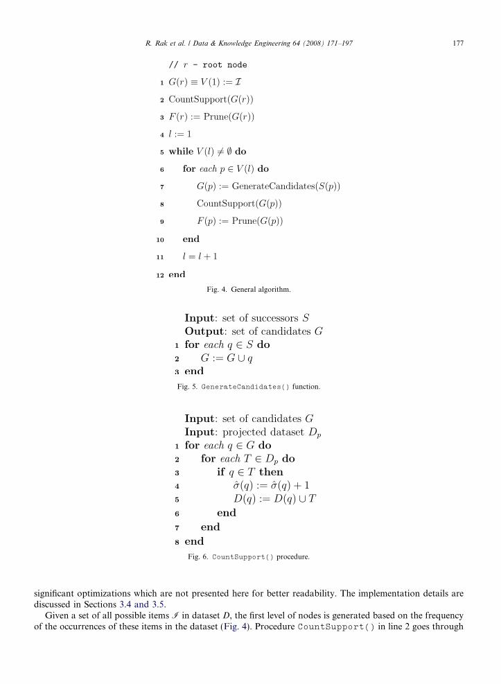
Fig. 4. General algorithm.

Fig. 5. GenerateCandidates() function.

Fig. 6. CountSupport() procedure.


significant optimizations which are not presented here for better readability. The implementation details arediscussed in Sections 3.4 and 3.5.

Given a set of all possible items I in dataset D, the first level of nodes is generated based on the frequencyof the occurrences of these items in the dataset (Fig. 4). Procedure CountSupport() in line 2 goes through

Fig. 7. Prune() function.


the dataset and increases support count for each node from the set passed to the function as an argument.Infrequent nodes are pruned (line 3) based on support threshold. Subsequent levels are created based on pre-ceding levels. The three functions GenerateCandidates(), CountSupport(), and Prune() (lines 7–9)are repeated for each node at the current level. (Note that nodes V(l) for l > 1 may have different parents.) Thealgorithm stops if there is no new level of nodes to generate further nodes from (the condition in line 5).

Details of function GenerateCandidates() are shown in Fig. 5. The function simply creates a copy ofa node and ties it with an appropriate parent.

Procedure CountSupport(), shown in Fig. 6, needs more attention. The existence of each candidate isverified against a projected dataset (lines 2–7). If a candidate exists in a currently processed transaction T (line3), its support count is increased by one (line 4), whereas T is added to candidate’s projected dataset D(q) (line5). Therefore the function not only counts support but also creates projected datasets.

Function Prune(), shown in Fig. 7, simply verifies the support count of each candidate and prunes thosethat do not satisfy a given support threshold.

The actual implementation counts the support and creates projected datasets using more advanced tech-niques. More specifically transactions are verified against the whole set of candidates G(p) at once and pro-jected datasets keep only references to transactions in dataset D which is discussed in details in Section 3.4.

The following section addresses adding class labels into the rule generation process.

3.2. Labels in the projected tree

This section focuses on building the complete rule tree, i.e., a tree containing both items and labels. Theeasiest way to include labels in a frequent itemset is to treat them as items, i.e., neglect distinction betweenitems and labels. However, this solution would result in a vast amount of association rules without a labeland rules containing labels only. In other words, there would be cases where creating a rule in the form ofX) C would be impossible due to the lack of either X or C. Although after pruning incomplete rules thissolution is undoubtedly correct, it is highly inefficient. For instance, in the tree shown in Fig. 3 if ‘‘1’’denotes a label and ‘‘2’’, ‘‘3’’, and ‘‘4’’ denote items, from the total of 15 rules only seven have a labeland at least one item. Using real datasets and n > 0 the number of complete rules, X) C, is significantlysmaller.

To avoid generation of unwanted rules both the tree and algorithm need to be modified. Similarly to items,we assume that there is an order between labels. We propose to implement the following constraints into thetree to efficiently generate association rules with class labels:

• The first level consists of nodes representing labels only.• The second level consists of nodes representing items only.• Levels three and higher consist of nodes representing both items and labels.• If nodes have the same parent, nodes representing items precede those representing labels.

root

A

2 3

2 3

3

1

B C

B C

B C C

C

B C

C

C

3 B

B C C

C

C B C

C

1 3 2

2 3

3 C C

C

C 3 C

C

C

B

21 3

3

3

3

C

2

Fig. 8. Multi-label ruleitem tree.


An example of a complete tree consisting of items and labels is depicted in Fig. 8. Labels and items aredenoted by capital letters and numbers, respectively.

Situating labels at the first level ensures that all rules have at least one label. Lack of labels at the secondlevel prevents from generating rules without items. Note that although the first level of labels is essential forbuilding further generations, it cannot be used to produce any rules by itself.

The algorithm for frequent itemset mining presented in the previous section must be modified to accommo-date for the class labels. However, it still can be used applying some modifications without giving up the intrin-sic characteristics of the algorithm. We observe that the second level candidates cannot be generated fromsuccessors S(p) of any first-level node p. Similarly the third level of nodes does not fully follow Candidate-

Generation() function. However, generation of the nodes of levels greater then three does comply with thefunction. This leads to the modifications of the basic algorithm as shown in Fig. 9.

The new algorithm consists of four parts. The first part builds the first level of nodes representing labels(lines 1–3). The second part (lines 4–8) assigns items to each first-level node. At this point it is possible to pro-duce fully qualified rules, X) C, consisting of exactly one item and one label.

Up to now each level greater than one is built based on its preceding level only. However, the generation ofthe third level involves two preceding levels. Given node p at level two, the third level candidates are generatedbased on successors S(p) as well as successors of p’s parent S(P(p)) (line 10). Levels four and higher are gen-erated in the same fashion as described in previous section (see Fig. 4).

3.3. Recurrent items

Recurrent items have been already defined in Section 2.1. A fragment of a tree consisting of recurrentitems and its corresponding set of ruleitems is shown in Fig. 10. To avoid ambiguity between item’s iden-tifier and a number of its occurrences, the latter one is put in round brackets, i.e., notations qixi and xi(qi)are equivalent.

The algorithm is adapted to take recurrent items into consideration by introducing one modification: a setof successors S(p) of node p is extended by this node. To further limit the number of candidates the followingconstraints must also be applied. For a given node p, for which candidate branches are to be created:

• if p 2 C then p must not be added to the list of successors, and• if p 2 I then p is added to the list of successors if and only if the number of p’s ancestors representing the

same item in the path from the root to p is less that the maximum number of occurrences of p per trans-action in a dataset.

Fig. 9. General algorithm for mining ruleitem tree.


Indeed, labels in a rule need to be distinct, and the maximum number of occurrences of any item in a rule-item cannot be more than the maximum number of occurrences of that item in any transaction. The latterlimitation requires the algorithm to store the information about a maximum number of occurrences of items.This can be simply achieved by the initial reading of a dataset when the algorithm builds the index of frequentitems.

3.4. Candidate test optimization

Most of the solutions related to the generate-and-test approach of frequent itemset mining rely on very sim-ple candidate test method. Each candidate itemset is verified against each transaction from a projected (or ori-ginal) dataset.

Let X = {x1,x2, . . .,xk} be a candidate k-itemset and T = {y1,y2, . . .,yl} be a transaction of length l. The eas-iest strategy to test the candidate would be to compare each item in X with every item in T. In the worst casescenario this results in k · l comparisons. If items in both X and T are ordered (the order in X is embedded intothe generated tree, whereas the order in T requires a single sort operation) then the complexity decreases to thesize of either a transaction or itemset, whichever is longer (in most real-life cases transactions are longer thanitemsets). This, however, has to be repeated |D(p)| times for every node p in the tree.

Instead of testing each itemset against every transaction we can again use the generated ruleitem treetogether with the projected datasets. Maintaining projected datasets allows for checking only the last item

1 2

2

A

3

3 B

2 3 3

2 3

2

B

a

b

Fig. 10. Fragment of (a) tree with recurrent items and (b) its corresponding set of ruleitems.


in an itemset represented by a node in G(p) for some p, since the remaining part of the itemset has been alreadyverified in the previous levels. We also observe that G(p) is ordered in the tree. Therefore we can test the entireG(p) against a transaction at once. However, now instead of testing whether X � T, the support of each itemxi 2 X is increased if xi = yj for any yj 2 T. Thus, our approach results in |G(P(p))| times smaller number ofoperations.

Procedure IncreaseSupportAndCreateProjDatasets(), shown in Fig. 11, performs the candidatetest described above. For any given set X, function Next(X) successively returns items from set X, one ateach call, with respect to order in X.

3.5. Dataset optimization

The algorithm distinguishes between two types of datasets: generic and projected. Generic dataset is readfrom a hard drive and stored in main memory. This dataset is kept at the root node of the ruleitem tree andused for a candidate test at the first level of the tree. Projected datasets are obtained from the generic datasetand used for candidate test at levels higher then one. This section discusses the optimization techniques forstorage and accessing both generic and projected datasets.

There are several different techniques of storing a dataset in the main memory. One possibility is tokeep transactions in the form of bit vectors so that each bit represents either the existence or absenceof an item. This allows for very fast candidate test if itemsets are kept in the same fashion. However, thissolution is memory consuming, especially when dealing with sparse data which is the case, e.g., in textcategorization.

Another solution is to keep items in a transaction in the form of a list. Although it slows down candidatetests, this structure is very often the only way to deal with large amount of sparse and highly dimensional data.

The proposed method uses item lists. To reduce the amount of required memory, the stored transactionsconsist of frequent items only. There are two methods to filter out the frequent items either by (1) readingthe complete transactions once into the main memory and next pruning infrequent items or (2) reading thecomplete transactions to compute item frequency values and then reading the data once again and storingin the main memory only the frequent items which are selected based on the counts computed during the first

Fig. 11. IncreaseSupportAndCreateProjDatasets() procedure.


reading. The first solution is faster because it reads the dataset only once. However, in some cases there mightnot be enough space to load the entire dataset.

Having the entire dataset in the main memory there is no need to copy transactions to the projected data-sets for every node. Therefore the projected datasets keep only references to the generic dataset. This signif-icantly reduces memory consumption.

Another optimization employed in the proposed algorithm is deleting projected datasets if they are nolonger needed. If level k + 1 has been created, the projected datasets of nodes at level k can be deleted.

4. The proposed algorithm

Two possible strategies can be used to explore the ruleitem tree either by using a breadth-first search or byusing a depth-first search. These strategies differ from each other with respect to the total number of projecteddatasets required to compute the rules. The two strategies are discussed in the following sections.

4.1. Breadth-first strategy

In breadth-first search approach the tree is explored level by level, i.e., level l + 1 of the tree is generatedonly if computations are completed for all nodes at level l. The basic mechanism of the breadth-first searchapproach has already been presented in the previous sections. Here we provide more details and discuss prosand cons of this approach.

Using the breadth-first search we can take advantage of an important property of the A priori algorithm: ifan itemset is not frequent its superset is not frequent either. Due to the fact that the tree is a representation ofitemsets, this property can be exploited to optimize the algorithm. Before going into details let us introduce aconcept of a base node:

Base node: Given node p and q such that q 2 G(p), we call node s 2 S(p) base node of q, denoted B(q), if node q

was directly generated from node s.

In order for the algorithm to comply with the A priori property, before generating (l + 1)-level node q for l-level node p from some successor s 2 S(p) it must verify whether node s belongs to frequent branches of p’s


(l � 1)-level base node, i.e. whether s 2 F(B(p)). This prevents from testing of nodes that are guaranteed not tobe be frequent, and thus saves time needed for candidate test operations. The new procedure for generatingcandidates, namely GenerateCandidatesBF(), is depicted in Fig. 12.

The breadth-first algorithm, shown in Fig. 13, begins with determining a set of the first-level frequent nodes.After employing dataset optimization, described in Section 3.5, this set is equal to the set of labels C, i.e., we

Fig. 12. GenerateCandidatesBF() function.

Fig. 13. Breadth-first algorithm.


assume that C consists of frequent labels only. For each node in the current level l set of candidates G(p) isgenerated (lines 5–11) following a procedure associated with level l of the tree (discussed in Section 3.2). Sup-port for each candidate is calculated and candidates’ projected datasets are created (lines 12–14) according tooptimized procedure described in 3.4. Finally, the infrequent candidates are pruned and dataset D(p) is deletedto release no longer needed portion of memory (lines 15–16). The procedure is repeated as long as newly gen-erated frequent nodes exist.

4.2. Depth-first strategy

The main drawback of the breadth-first algorithm is that the number of projected datasets is equal to thenumber of nodes in the current level l plus one dataset at level l � 1. For a large number of items and lowsupport threshold values the tree may become very wide which may result in substantial memory consump-tion. A depth-first search approach addresses this problem. In this case branches are created path-wise, i.e.,for a given node p a set of frequent nodes F(p) is found and for each such node q 2 F(p) the procedure asfor p is recursively repeated until the last level of the tree is reached.

After reaching the last level as shown in the example, the last but one is mined, etc.A complete psuedocode of the proposed depth-first search algorithm is shown in Fig. 14.Function DepthFirst() is performed for each frequent label. The function itself generates candidates

following, again, the level-dependent procedure described in Section 3.2 (Fig. 14b, lines 3–12). Note that indepth-first strategy it is impossible to determine base node B(p) for any given p during the process of gener-ating candidates, simply because base node B(p) is yet to be discovered. Therefore, GenerateCandi-dates() function does not follow GenerateCandidatesBF() depicted in Fig. 12. After support foreach candidate is calculated, projected datasets are created, and infrequent candidates are pruned (lines 10–13), DepthFirst() function is performed recursively for each frequent candidate (lines 14–16). The memoryoccupied by the projected dataset can be released only after all frequent branches of the currently performednode are mined (line 17).

The maximum number of projected datasets held in main memory at the same time depends now on thenumber of levels and is equal to

Pni¼1jGðpiÞj where n is the number of levels in the currently mined path. Note

that |G(pi)| 6 |G(pi�1)|.The number of levels depends on the statistic features of a dataset and a given support threshold. The lower

the threshold or the longer patterns in data, the bigger the number of levels and longer rules. Nevertheless, themaximum number of levels can never exceed the number of items, which gives a significant reduction in thenumber of projected datasets when compared to the exponential growth of projected datasets in the breadth-first strategy. A closer look at the complexity of these two algorithms is provided in the next section.

4.3. Complexity and limitations

This section discusses the complexity of the algorithms and their limitations. We compare our breadth-firstand depth-first algorithms to each other as well as to our implementation of tree-based A priori (brieflydescribed in Section 5).

4.3.1. Computational complexity

Runtime complexity depends on the number of nodes (candidates) in the tree and the computation timeneeded for each node. We address each of them separately and multiply the resulting complexities to obtainthe total complexity. For simplicity (without loss of generality), let us treat labels in the same fashion as items.

The size of the tree depends on the number of items (and labels) and a pruning factor, i.e., the differencebetween the number of candidates and the number of frequent items. For simplicity of further analysis letus assume that this difference is constant for all groups of candidates, i.e., G(p) � F(p) = k for each node p,where k = const.

This results in the following formula for the size of tree T (excluding the root node):

jTkðnÞj ¼ F kþ1ðnþ 1Þ � 1 ð3Þ

Fig. 14. Depth-first algorithm.


where n is the number of items (and labels) and Fm is a generalized Fibonacci number, which, in its combina-torial representation [17], is:

F mðnÞ ¼Xnþm�2

mb c

i¼0

nþ m� 2� ðm� 1Þii

� �ð4Þ


In the worst case scenario (e.g., a crude dataset containing only one transaction or a set of exactly the sametransactions) the size of the tree is 2n � 1 (which can be derived from (3) for k = 0). This exponential growthbecomes weaker for greater values of k, and the complexity can be expressed as O(cn) for some constant c,where c = 2 for k = 0 and converges to 1 with increasing values of k.

If, however, pruning factor k is relative to the number of items n (for instance, k = n/2, i.e., a situationwhere always a half of first-level candidates is frequent) it is expected that for certain relations of k and n

the computational complexity will become lower than O(cn). Let us analyze the following recursive formulafor the size of the tree:

jTkðnÞj ¼n if n 6 k þ 1;Pn�k�1

i¼1 jTkðiÞj þ n if n > k þ 1;

�ð5Þ

This formula is derived directly from the visual representation of the tree (see Section 3). Eliminating therecursion in (5) results in the following formula dependent on the relation between k and n:

jTkðnÞj ¼n if n 6 3kþ1

2;

2n�3k�12

k þ n if 3kþ12< n 6 2k þ 1;Pn�2k�1

i¼1 F kþ1ðn� 2k � iÞiþ 2n�3k�12

k þ n if n > 2k þ 1;

8><>: ð6Þ

From (6) we can observe that the bigger the difference between n and k, the bigger the tree growth rate. Withconstant k and increasing n the size of the tree grows from O(n) (the first case) to O(n2) (the middle case) toO(cn) (the latter case, where mainly the sum of generalized Fibonacci numbers dictates the growth). Thus, if k

is relative to n the tree growth rate can decrease significantly. For instance, to continue with the previousexample, for k = n/2 the tree growth becomes quadratic.

Let us now analyze the complexity of operations that need to be performed at each node of the tree. Fromthe algorithms presented in Sections 3 and 4 we see that each node (a candidate) requires the following oper-ations to be performed: (1) generation, (2) counting support, and (3) pruning. Generation is only a matter ofadding a single item to the tree. The complexity of counting support was already discussed in Section 3.4 and isproportional to jDðpÞj

jGðP ðpÞÞj jT j for node p and transaction T, i.e., it takes |G(P(p))| times less time than supportcounting in other algorithms. Pruning is only a simple if statement comparing two numbers and, if true, delet-ing the node.

The difference between the depth-first and breadth-first search algorithms, as described in Sections 4.1 and4.2, lies in generating less candidates for the latter one (although it yields additional comparisons). However,the asymptotic complexity of those two algorithms remains the same. Thus, the majority of time is spent on thecandidate test (counting support). The range of denominator |G(P(p))| is 1 to n with lower values on deeperlevels of the tree. However, numerator |D(p)|, bounded by n̂ and |D|, also decreases at the same time. Althoughthe asymptotic upper bound of the candidate test is still O(m), where m = |D|, there is a substantial reductionin the number of candidate tests when compared to the algorithms of other researchers due to the decreasingsize of projected datasets D(p) and performing aggregated (vs. one node at a time) tests.

The total computational complexity of the proposed algorithms equals O(nm), O(n2m), and O(cnm) depend-ing on the relation between k and n. It varies from being linear to quadratic to exponential (the first two only ifthe pruning factor depends on the number of items) with respect to the number of items (and labels) with theconstant number of transactions, and linear with respect to the number of transactions with the constant num-ber of items (and labels). Although the latter one is scalable, the tree-size-dependent complexity imposes cer-tain limitations on our algorithms: they will not scale well in situations with long patterns in data (very similartransactions) or/and very small support thresholds. In both such situations the pruning factor will be close tozero, which, in turn, will ‘‘trigger’’ exponential growth in the number of operations. However, in somedomains such as text categorization, the pruning factor is relatively high, and thus, the expected complexityshould remain at most quadratic.

4.3.2. MemoryDue to the fact that our proposed algorithms keep projected datasets their memory consumption is obvi-

ously higher than, for instance, the one of A priori, which keeps only a dataset and the tree nodes in main


memory, i.e., its memory consumption is proportional to jDj þ jTj. However, breadth-first and depth-firstalgorithms differ from each other in the number of projected datasets they keep (discussed in Sections 4.1and 4.2). Thus, memory usage is proportional to:

• jDj þ jTj þP

p2V maxjDðpÞj for the breadth-first algorithm, and

• jDj þ jTj þPbnþk

kþ1c�1

i¼0

Pq2GðpiÞjDðqÞj for the depth-first algorithm,

where n, as before, is the number of items (and labels), pi is an ith node of the currently searched path in thetree (with p0 being the root node), and Vmax is a set of nodes at the widest level of the tree with the followingcardinality (assuming the concept of pruning factor as described in Section 4.3.1):

jV maxj ¼ max06i6bnþk

kþ1c

nþ k � ki

i

� �: ð7Þ

The above equation is obtained from (4) and is equal to the maximum component of the sum for Fk+1(n + 1)in (4), which can be estimated as O(cn) for constant c, 1 < c < 2. The number of nodes in G(pi) for each pi in thepath is of O(n2). Based on these estimates and those made in Section 4.3.1 the asymptotic complexity, in termsof memory usage, can be written as:

• O(m) + O(cn) + O(cn)O(m), and• O(m) + O(cn) + O(n2)O(m),

for the breadth-first and depth-first algorithms, respectively. Thus, the projected datasets increase memoryusage (when compared to the A priori) exponentially and quadratically with the increasing number of items(and labels) for the breadth-first and depth-first algorithms, respectively.

5. Experiments

A number of experiments exploiting a wide space of parameter values and input data was performed toevaluate runtime and memory consumption of the proposed algorithm for the multi-label associative-classifi-cation with recurrent items.

We also implemented a priori-like version of associative-classification rule generator and compared it withthe proposed algorithm. This algorithm works in similar fashion to the one described in [20]. The main dif-ference is that it is based on the ruleitem tree as a ruleitem representation. We refer to this algorithm as A

priori, whereas the two versions of the proposed algorithm, breadth-first and depth-first projected, are referredas BF-TP and DF-TP, respectively.

Although two measures indicating the strength of rules, namely support and confidence, are usually used asparameters of association-rule mining, only support is used in this paper. The confidence, though a very sig-nificant parameter, is usually often omitted (like in frequent pattern mining) because it does not directly influ-ence the number of generated rules but is only used to prune some of them.

5.1. Experimental setup

Although many researchers demonstrate complexity of their algorithms using synthetic data or small single-label corpora [20,19,35,34], these data cannot be used in case of the proposed method. First of all, datasetsused to verify frequent pattern mining methods lack labels which are an intrinsic part of associative-classifi-cation rule generation. Secondly, our intention is to primarily use this algorithm for text categorization. There-fore, we chose OHSUMED [16] and RCV1 [18] corpora which are standard benchmarks in the textcategorization and, most importantly, provide multi-label transactions.

OHSUMED [16] is a corpus of 348,543 records extracted from the MEDLINE, National Library ofMedicine’s (NLM) database consisting of approximately 13 million article references to biomedical journalarticles, limited to 5 years: 1987–1991. Each document is assigned to Medical Subject Headings (MeSH),


NLM’s controlled vocabulary thesaurus consisting of medical terms at various levels of specificity. We used amodified version of this collection described in [31]. The original collection was reduced to documents thathave both title and abstract which resulted in the total of 233,445 documents. Over 22,000 headings arrangedin 11-level structure were generalized to the second level resulting in the total of 114 class labels [31]. We referto this dataset as ohsumed-gen2.

The second dataset, RCV1 [18], is much larger and contains 804,414 news stories from Reuters. Fromthroughout several dimensions of labels available for this collection we chose the most commonly used andadequate for our goal, 103 labels of ‘‘topics’’. Each Reuters’s news story is assigned to at least one topic thatcategorizes this story. We refer to this dataset as rcv1-topics.

Both datasets are summarized in Table 2.The proposed algorithm is evaluated with respect to several performance measures such as runtime, mem-

ory consumption, and scalability. Several sets of experiments for various sizes of the datasets and supportthreshold values were performed, and both single- and multi-label rules were generated. The complete exper-imental setup is shown in Table 3.

The experiments were performed on a PC with a 2 GHz Pentium IV processor and 1.5 GB of RAM. Run-time is measured excluding the time of reading a dataset from a hard drive. The reading time depends on thesize of a dataset only, i.e., it is indifferent to parameters and algorithms chosen, and ranges from several sec-onds for the smallest datasets used to several minutes for the biggest datasets.

5.2. Runtime

Fig. 15 shows the runtime values of the algorithms on the two datasets. Due to space limitations, runtimeis shown only for datasets with 100,000 transactions and various support threshold values. Performance onthe entire range of dataset sizes is analyzed in Section 5.4 that evaluates the scalability of the algorithm.Fig. 15a, c, e, and g shows the runtime in the function of a support threshold (note the reverse order).A priori is definitely slower than both BF-TP and DF-TP algorithms when exploring low values of the sup-port threshold. We observe that the runtimes have tendency to rapidly grow with respect to the decreasingsupport. However, the number of rules generated grows nonlinearly with increasing value of the supportthreshold. Fig. 15b, d, f, and h shows the same runtime in function of the number of generated rules.The axes are scaled logarithmically to help visualize all points on the graph. The three algorithms show lin-ear relationship between runtime and the number of rules. The dotted line on the graph is a linear approx-imation (in a least squares sense) for the DF-TP algorithm. Both BF-TP and DF-TP require significantlyless runtime to generate the same number of rules when compared with A priori. The coefficients of linearapproximations for the rcv1-topics dataset are {0.63, 114}, {0.019, 12}, and {0.021, 12} for A priori, BF-TP,and DF-TP, respectively, where {a,b} indicates coefficients for the linear approximation f(x) = ax + b.

Table 2Dataset statistics

Dataset Size Number of labels Number of words

Total l r Total l r

ohsumed-gen2 233,445 114 9.8 3.1 99,775 95.6 40.62rcv1-topics 804,414 103 3.2 1.4 288,062 123.9 110.3

l, average per transaction; r, standard deviation.

Table 3Experimental setup

Dataset Size (Transaction number) [k] Support threshold [%]

ohsumed-gen2 12.5, 25, 50, 100, 200 2, 3, 4, 8, 12, 16, 20rcv1-topics 25, 50, 100, 200, 400, 800 2, 3, 4, 8, 12, 16, 20

51015200

2000

4000

6000

8000

Support threshold [%]

Tim

e [s

]

ohsumed–gen2 (size=100k, multilabel)AprioriBF–TPDF–TP

102

103

104

102

104

Number of rules

Tim

e [s

]

ohsumed–gen2 (size=100k, multilabel)AprioriBF–TPDF–TPlinear aprox.

51015200

1000

2000

3000

4000

5000


Tim

e [s

]

rcv1–topics (size=100k, multilabel)AprioriBF–TPDF–TP

101 102 103 104

100

102

104

Number of rules

Tim

e [s

]

rcv1–topics (size=100k, multilabel)AprioriBF–TPDF–TPlinear aprox.

51015200

1000

2000

3000

4000

5000


Tim

e [s

]

ohsumed–gen2 (size=100k, singlelabel)AprioriBF–TPDF–TP

101

102

103

100

102

104

Number of rules

Tim

e [s

]

ohsumed–gen2 (size=100k, singlelabel)AprioriBF–TPDF–TPlinear aprox.

51015200

1000

2000

3000

4000


Tim

e [s

]

rcv1–topics (size=100k, singlelabel)AprioriBF–TPDF–TP

101

102

103

104

100

102

104

Number of rules

Tim

e [s

]

rcv1–topics (size=100k, singlelabel)AprioriBF–TPDF–TPlinear aprox.

a b

c d

e f

g h

Fig. 15. Runtime.


Although the three considered algorithms are characterized by the same linear asymptotic complexity withrespect to runtime, linear extrapolation to 50,000 rules shows that it takes almost 9 h to generate rules usingA priori and only about 16 min using BF-TP.

The difference in runtime between A priori and the two proposed algorithms is a result of storing pro-jected datasets in case of the two latter algorithms. The difference between BF-TP and DF-TP is most likely


a result of a lower number of candidates in BF-TP. BF-TP limits this number during generation of nodesusing information from upper levels of the tree, which is not available in case of DF-TP (for details referto Section 4.1).

If we treat the decreasing support threshold as the way to increase the number of items in the mining pro-cess, we observe that the obtained results fully comply with complexity estimates (O(cn)) elaborated in Section4.3.1.

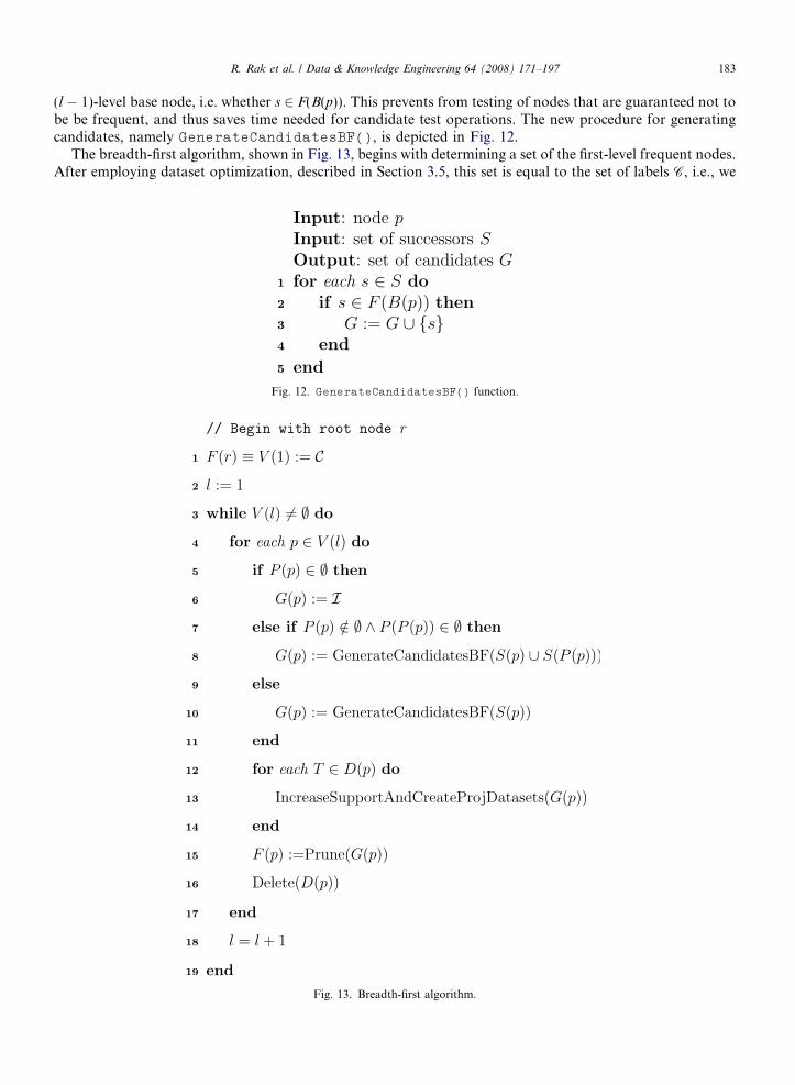
5.3. Memory consumption

Memory characteristics, shown in Fig. 16, are similar to those for the runtime, i.e., memory consump-tion rapidly grows with lower values of the support threshold (Fig. 16a, c, e, and g). However, in contrastto the runtime results, the algorithms performing faster, i.e., BF-TP and DF-TP, require more memorythan the slowest, A priori. In fact, A priori’s memory consumption changes only slightly even for a lowsupport threshold when compared to BF-TP and DF-TP. Although BF-TP and DF-TP require comparableamount of memory for higher values of support threshold, the former one requires significantly more mem-ory for medium and low values of support. Nevertheless, the three algorithms are characterized by approx-imately linear characteristic between memory consumption and the number of rules, as shown in Fig. 16b,d, f, and h.

Since A priori does not store projected datasets, the size of memory it requires is dependent only on thenumber of generated rules. In case of both BF-TP and DF-TP relatively large memory consumption is dueto storing projected datasets. However, we note that DF-TP consumes significantly less memory than BF-TP when generating a large number of rules. For DF-TP, the number of projected datasets depends on thedepth of the tree and not, as in case of BF-TP, on its width. As a consequence, since lowering support thresh-old results in creation of wider, rather than deeper, ruleitem trees, DF-TP is characterized by worse memoryconsumption when compared to BF-TP.

Again, treating the decreasing support threshold as the way to increase the number of items, the obtainedresults confirm our estimates made in Section 4.3.2. It also confirms the limitations of our algorithms: either alow support threshold or long patterns in data, i.e., the situation where very similar transactions yield a largenumber of patterns even if a support threshold is high, will result in numerous nodes in the tree and potentiallylarge projected datasets (or rather references to the generic dataset as discussed in Section 3.5) on those nodes.This, in turn, may result in memory overflow. Nevertheless, setting a reasonable support threshold is left touser’s disrection (e.g., buliding a rule-based classification model that consists of more rules than transactionsmay raise some doubts on usefullness of such a model) and becomes an engineering task itself.

5.4. Scalability

Scalability test was performed by iteratively increasing the number of transactions in the input dataset andmeasuring the corresponding results. The results are shown in Fig. 17. Both runtime and memory consump-tion indicate linear relation with the growing number of transactions (as estimated in Sections 4.3.1 and 4.3.2).Similarly to the previous results, BF-TP and DF-TP show comparable scalability and are superior to A prioriwith respect to runtime (Fig. 17a, c, e, and g). For instance, for the multi-label rcv1-topics dataset and thesupport threshold of 4% it takes about 237 seconds for A priori to generate rules from 25,000 transactionsand about 12 s for DF-TP. For larger 800,000-transaction dataset A priori needs almost two hours comparedto about 7 min for DF-TP.

On the other hand, memory consumption diagrams (Fig. 17b, d, f, and h) shows the opposite relation.Memory usage for A priori is almost constant, whereas for TP-algorithms, the required memory is linearlyincreasing with the increasing number of transactions.

Assuming uniform distribution of words in a dataset, the number of rules generated with the same supportthreshold should be virtually the same for any subset of the dataset. This implies that the ruleitem tree struc-ture be almost identical. That is why A priori use nearly the same amount of memory for different datasetsizes. Since TP-algorithms need to keep projected datasets, their memory consumption increases linearly withthe size of the generic dataset.

51015200

100

200

300

400


Mem

ory

[MB

]

ohsumed–gen2 (size=100k, multilabel)

AprioriBF–TPDF–TP

102 103 104

102

100

102

Number of rules

Mem

ory

[MB

]

ohsumed–gen2 (size=100k, multilabel)AprioriBF–TPDF–TPlinear aprox.

5101520

0

50

100

150

200


Mem

ory

[MB

]

rcv1–topics (size=100k, multilabel)


101 102 103 104

102

100

102

Number of rules

Mem

ory

[MB

]

rcv1–topics (size=100k, multilabel)AprioriBF–TPDF–TPlinear aprox.

5101520

0

50

100

150

200


Mem

ory

[MB

]

ohsumed–gen2 (size=100k, singlelabel)


101 102 103

102

100

102

Number of rules

Mem

ory

[MB

]

ohsumed–gen2 (size=100k, singlelabel)AprioriBF–TPDF–TPlinear aprox.

5101520

0

50

100

150

200


Mem

ory

[MB

]

rcv1–topics (size=100k, singlelabel)


101 102 103 104

102

100

102

Number of rules

Mem

ory

[MB

]

rcv1–topics (size=100k, singlelabel)AprioriBF–TPDF–TPlinear aprox.

a b

c d

e f

g h

Fig. 16. Memory consumption (multi-label rules).


5.5. Single- vs. multi-label rule generation

The results discussed in the previous sections show that both single-label rule generation and multi-labelrule generation preserve the same asymptotic complexity and relations between the three considered

0.5 1 1.5 2

x105

0

500

1000

1500

2000

2500

Dataset size

Tim

e [s

]

ohsumed–gen2 (support=4%, multilabel)AprioriBF–TPDF–TP

0.5 1 1.5 2

x105

0

50

100

150

200

250

Dataset size

Mem

ory

[MB

]

ohsumed–gen2 (support=4%, multilabel)AprioriBF–TPDF–TP

1 2 3 4 5 6 7 8

x105

0

1000

2000

3000

4000

Dataset size

Tim

e [s

]

rcv1–topics (support=4%, multilabel)AprioriBF–TPDF–TP

1 2 3 4 5 6 7 8

x105

0

100

200

300

Dataset size

Mem

ory

[MB

]

rcv1–topics (support=4%, multilabel)AprioriBF–TPDF–TP

0.5 1 1.5 2

x105

0

500

1000

1500

Dataset size

Tim

e [s

]

ohsumed–gen2 (support=4%, singlelabel)AprioriBF–TPDF–TP

0.5 1 1.5 2

x105

0

50

100

150

Dataset size

Mem

ory

[MB

]

ohsumed–gen2 (support=4%, singlelabel)AprioriBF–TPDF–TP

1 2 3 4 5 6 7 8

x105

0

1000

2000

3000

Dataset size

Tim

e [s

]

rcv1–topics (support=4%, singlelabel)AprioriBF–TPDF–TP

1 2 3 4 5 6 7 8

x105

0

100

200

300

Dataset size

Mem

ory

[MB

]

rcv1–topics (support=4%, singlelabel)AprioriBF–TPDF–TP

a b

c d

e f

g h

Fig. 17. Scalability (multi-label rules).


algorithms. Fig. 18 shows a summarized comparison of the cost of generating multi-label rules in relation tosingle-label rules with respect to the number of rules generated and runtime. For the same support thresholdthe two types of rule generation differ in the number of generated rules. This difference is especially visible withthe low values of support threshold. For instance, setting the support threshold value to 4% results in gener-ation of about two and a half times more multi-label rules than single-label rules with only about 80% increase

51015200

50

100

150size=100k


Rul

e in

crea

se [%

] rcv1–topicsohsumed–gen2

51015200

50

100

150size=100k


Tim

e in

crea

se [%

] rcv1–topicsohsumed–gen2

a b

Fig. 18. Increase (a) in the number of rules between multi-label and single-label rules, and (b) in runtime to generate multi-label rules inrelation to single-label rules.


in runtime. (The difference between the two datasets used in experiments is a consequence of their class labeldistribution, i.e., the average number of labels per transaction is significantly higher in the ohsumed-gen2 data-set than in the rcv1-topics dataset (see Table 2).) This shows that the generation of multi-label rules, that aresupersets of single-label rules, is feasible with relatively low cost when compared to the generation of single-label rules.

5.6. Analysis of generated rules

Table 4 shows several rules for each of the dataset used in the experiments. All item names are shown intheir stemmed form (e.g., studi, compan, and pric), which in some cases may become ambiguous. The presentedrules were chosen in a way to show the variety of forms they can take and to be comprehensible to non-experts. There are rules with one item and one label (rules (ii), (iv), (vi), and (x)), with multiple items andone label (rules (i), (iii), (ix), and (xii)), with one item and multiple labels (rules (vii) and (viii)), and finallymultiple items and labels (rules (v), (xi), and (xiii)). As expected, introducing recurrent items increases the con-fidence of the rule, decreasing support at the same time (compare rules (v) and (vii)). Rules with high supportand low confidence (such as rule (viii)) signal that rules’ items are commonly used throughout most of the clas-ses and may be considered to be added to the list of stop words, i.e., the list of words that appear frequently but

Table 4Examples of discovered rules in (a) ohsumed-gen2 and (b) rcv1-topics datasets

Rulea Support (%) Confidence (%)

(a) ohsumed-gen2(i) rat(2)! Animals [B01] 5.30 99.96(ii) bondr! Animals [B01] 4.17 99.86(iii) effect, studi, control! Animals [B01] 4.29 99.35(iv) children! Persons [M01] 4.64 95.71(v) tumor(2)! Animals [B01], Neoplasms [C04] 4.11 93.80(vi) tumor!Neoplasms [C04] 6.13 89.09(vii) tumor! Animals [B01], Neoplasms [C04] 6.10 82.94(viii) studi! Persons [M01], Animals [B01], Investigative Techniques [E05] 12.26 30.75

(b) rcv1-topics(ix) million, net, profit! Corporate/Industrial 4.02 92.28(x) compan! Corporate/Industrial 21.84 78.50(xi) net, profit! Corporate/Industrial, Performance 4.19 78.09(xii) net, profit! Performance 4.19 78.09(xiii) market, pric! Commodity markets, Markets 4.00 31.03

a Number in parentheses denotes recurrence.


are irrelevant to classification. Clearly, the most valuable rules, from predictive point of view, are those withhigh support and high confidence. However, in most cases such rules are of no avail from descriptive point ofview as they usually carry obvious knowledge (see rule (x)). Thus, experts may be more interested in rules withhigh confidence disregarding their support at the same time (rule (ii) may be a candidate).

5.7. Classification

Although the main focus of this paper is the generation of association rules that can be used in associative-classification, we also demonstrate classification capabilities of the generated rules. We compared the classifi-cation accuracy of our method to recent results presented by Thabtah et al. [33]. That paper proposed amultiple-label associative-classification algorithm MMAC, and showed its accuracy on several benchmarkdatasets from the well-known UCI repository [23]. The authors compared their own MMAC algorithm tothree other classifiers including a decision-tree-based algorithm PART [9], rule-based RIPPER [5], and anassociative-classification algorithm CBA [20]. The four algorithms and ours alike are based on descriptive(human-interpretable) models. From the total of 19 datasets used in [33] we discarded one, namely Autos, sincewe were not able to identify an actual class attribute used by the authors.

Based on the rules generated using our algorithm (constrained by support and confidence thresholds) weapplied several techniques to classify instances. For each instance a set of rules that matched the instancewas chosen. This set of rules was further ranked according to either rules’ confidence or cosine measure beingan angle between a rule and instance represented by their vector models. The class from a rule with the highestscore (biggest confidence or smallest angle) was then assigned to the instance. In case where there was no rulesmatching the instance, the default class was always chosen. In order to generate rules for unevenly distributeddatasets we used a technique that generates rules based on a class-size-dependent support threshold, i.e., rulei-tems are pruned based on the support threshold proportional to the size of a class they include.

Eventually, the experiments were performed using a 10-fold cross validation technique with the followingparameters: (1) a support threshold, (2) a confidence threshold, (3) class-size-dependent thresholding (eitherswitched on or switched off), and (4) either a confidence-based or cosine-measure-based rank. This set ofparameters was tuned to maximize accuracy for a given dataset within 10-fold cross validation regime. Impos-ing cross validation ensures that the generated rules are general enough to avoid overfitting to a given trainingset – testing set pair. From rule expressiveness point of view it basically means less or/and shorter rules.

Table 5Comparison accuracy of five associative-classification algorithms

PART RIPPER CBA MMAC ACRI

Tictac 92.58 97.54 98.60 99.29 99.90Contact-lenses 83.33 75.00 66.67 79.69 85.00Led7 73.56 69.34 72.39 73.20 72.72Breast-cancer 71.32 70.97 68.18 72.10 74.00Weather 57.14 64.28 85.00 71.66 65.00Heart-c 81.18 79.53 78.54 81.51 83.46Heart-s 78.57 78.23 71.20 82.45 92.69Lymph 76.35 77.70 74.43 82.20 82.24Mushroom 99.81 99.90 98.92 99.78 95.57Primary-tumor 39.52 36.26 36.49 43.92 51.50Vote 87.81 87.35 87.39 89.21 94.10Crx 84.92 84.92 86.75 86.47 86.36Sick 93.90 93.84 93.88 93.78 93.88Balance-scale 77.28 71.68 74.58 86.10 83.45Breast-w 93.84 95.42 94.68 97.26 94.11Hypothyroid 92.28 92.28 92.29 92.23 95.22Zoo 91.08 85.14 83.18 96.15 90.00Kr-vs-kp 71.93 70.24 42.95 68.75 66.07

Average 80.36 79.42 78.12 83.10 83.63

Table 6Comparison of algorithms

Measurement Algorithm A priori Breadth-first

Runtime Breadth-first ++Depth-first ++ �

Memory Breadth-first ��Depth-first � ++

Scalability – runtime Breadth-first ++Depth-first ++ �

Scalability – memory Breadth-first ��Depth-first � ++

+, better; ++, far better; �, comparable; �, worse; ��, far worse.


The results for the best sets of parameters (tuned for each dataset individually) are shown in Table 5. Fromthe total of the five presented classifiers, our classifier performed the best in terms of the average classificationaccuracy. Performing a paired t-test shows that the differences are statistically significant (at the 95% confi-dence) in all cases but one, MMAC. Won-tied-loss records of our classifier against PART, RIPPER, CBA,and MMAC are 13-0-5, 15-0-3, 13-1-4, and 10-0-8, which again confirm superior performance of the proposedmethod over the other classifiers. The class-size-dependent thresholding technique proved to be successfulwhen dealing with multi-class, unevenly distributed datasets, such as Primary tumor (22 classes) for whichour classifier outperformed others by almost 8%. The main difference in generating rules between our algo-rithm and the best performing other associative-classification algorithm MMAC is that MMAC iterativelygenerates sets of single-label rules to eventually form a set of multi-label rules, whereas the proposed algorithmcreates multi-label rules at once, based on the projection tree.

6. Summary and conclusions

In this paper, we presented the design of an algorithm for generation of multi-label recurrent-item associa-tive-classification rules. The experimental results showed superior performance of the proposed breadth-firstand depth-first tree-projected algorithms over the A priori-like algorithm with respect to runtime. As expected,memory consumption is bigger for the proposed tree-projected algorithms than for the A priori-like algorithmdue to usage of projected datasets to generate rules. Although this difference is significant for the breadth-firstsearch, the memory characteristics indicate significantly better (smaller) memory consumption for the depth-first algorithm. The comparison of the three algorithms is summarized in Table 6. The comparison shows thatthe proposed depth-first search multi-label association classification rule generation algorithm provides thebest balance by being characterized by low runtime and moderate memory consumption. The proposedmethod is the first to address generation of multi-label association rules and achieves performance that is com-parable to a single-label rule generation. In short, we showed that the added value of multi-label rules comeswith a reasonably low cost in terms of both runtime and memory consumption. The algorithms scale linearlywith respect to the dataset size for both runtime and memory usage. Although complexity with respect to thenumber of items may become exponential (for frequent and long patterns), we showed several tree-based tech-niques to significantly slow down this growth, which makes our algorithms, and especially the depth-first strat-egy, more efficient than those of other researchers.

References

[1] R. Agarwal, R. Srikant, Fast algorithms for mining association rules, in: Proceedings of the International Conference on Very LargeData Bases, 1994, pp. 487–499.

[2] R.C. Agarwal, C.C. Aggarwal, V.V.V. Prasad, A tree projection algorithm for generation of frequent item sets, Journal of Paralleland Distributed Computing 61 (3) (2001) 350–371.

[3] E. Baralis, P. Garza, Majority classification by means of association rules, in: Knowledge Discovery in Databases: PKDD 2003, 2003,pp. 34–46.


[4] R.A. Calvo, J.-M. Lee, X. Li, Managing content with automatic document classification, Journal of Digital Information 5 (2) (2004).[5] W.W. Cohen, Fast effective rule induction, in: Proceedings of the 12th International Conference on Machine Learning, July 1995, pp.

115–123.[6] W.W. Cohen, Y. Singer, Context-sensitive learning methods for text categorization, ACM Transactions on Information Systems 17

(2) (1999) 141–173.[7] S. Cong, J. Han, J. Hoeflinger, D. Padua, A sampling-based framework for parallel data mining, in: Proceedings of the 10th

ACM SIGPLAN Symposium on Principles and Practice of Parallel Programming, ACM Press, New York, NY, USA, 2005, pp.255–265.

[8] G. Dong, X. Zhang, L. Wong, J. Li, Caep: classification by aggregating emerging patterns, in: Discovery Science, 1999, pp. 30–42.[9] E. Frank, I.H. Witten, Generating accurate rule sets without global optimization, in: Proceedings of the 15th International

Conference on Machine Learning, 1998, pp. 144–151.[10] B. Gao, T.-Y. Liu, G. Feng, T. Qin, Q.-S. Cheng, W.-Y. Ma, Hierarchical taxonomy preparation for text categorization using

consistent bipartite spectral graph co-partitioning, IEEE Transactions on Knowledge and Data Engineering, Special Issue on DataPreparation (2005) 41–50.

[11] V. Guralnik, G. Karypis, Parallel tree-projection-based sequence mining algorithms, Parallel Computing 30 (4) (2004) 443–472.[12] J. Han, J. Pei, Mining frequent patterns by pattern-growth: methodology and implications, SIGKDD Explorations Newsletter 2 (2)

(2000) 14–20.[13] J. Han, J. Pei, B. Mortazavi-Asl, Q. Chen, U. Dayal, M.-C. Hsu, Freespan: frequent pattern-projected sequential pattern mining, in:

Proceedings of the Sixth ACM SIGKDD International Conference on Knowledge Discovery and Data Mining, ACM Press, NewYork, NY, USA, 2000, pp. 355–359.

[14] J. Han, J. Pei, Y. Yin, Mining frequent patterns without candidate generation, in: Proceedings of the 2000 ACM SIGMODInternational Conference on Management of Data, ACM Press, New York, NY, USA, 2000, pp. 1–12.

[15] J. Han, J. Pei, Y. Yin, R. Mao, Mining frequent patterns without candidate generation: a frequent-pattern tree approach, DataMining and Knowledge Discovery 8 (1) (2004) 53–87.

[16] W. Hersh, C. Buckley, T.J. Leone, D. Hickam, Ohsumed: an interactive retrieval evaluation and new large test collection for research,in: Proceedings of the 17th Annual International ACM SIGIR Conference on Research and Development in Information Retrieval,Springer-Verlag New York Inc., New York, NY, USA, 1994, pp. 192–201.

[17] S.T. Klein, Combinatorial representation of generalized fibonacci numbers, Fibonacci Quarterly 29 (1991) 124–131.[18] D.D. Lewis, Y. Yang, T. Rose, F. Li, Rcv1: a new benchmark collection for text categorization research, Journal of Machine

Learning Research 5 (2004) 361–397.[19] W. Li, J. Han, J. Pei, Cmar: accurate and efficient classification based on multiple class-association rules, in: Proceedings of the IEEE

International Conference on Data Mining, 2001, pp. 369–376.[20] B. Liu, W. Hsu, Y. Ma, Integrating classification and association rule mining, in: Knowledge Discovery and Data Mining, 1998, pp.

80–86.[21] T.-Y. Liu, Y. Yang, H. Wan, H.-J. Zeng, Z. Chen, W.-Y. Ma, Support vector machines classification with very large scale taxonomy,

SIGKDD Explorations, Special Issue on Text Mining and Natural Language Processing (2005).[22] T.-Y. Liu, Y. Yang, H. Wan, Q. Zhou, B. Gao, H.-J. Zeng, Z. Chen, W.-Y. Ma, An experimental study on large-scale web

categorization, in: WWW ’05: Special Interest Tracks and Posters of the 14th International Conference on World Wide Web, ACMPress, New York, NY, USA, 2005, pp. 1106–1107.

[23] D. Newman, S. Hettich, C. Blake, C. Merz, Uci repository of machine learning databases, 1998.[24] K. Ong, W. Ng, E. Lim, Mining multi-level rules with recurrent items using fp’-tree, in: Proceedings of the Third International

Conference on Information, Communications and Signal Processing, Singapore, October 2001.[25] J. Pei, Pattern-growth methods for frequent pattern mining, Ph.D. Thesis, Simon Fraser University, June 2002.[26] J. Pei, J. Han, B. Mortazavi-Asl, H. Pinto, Q. Chen, U. Dayal, M.-C. Hsu, Prefixspan: mining sequential patterns efficiently by prefix-

projected pattern growth, in: Proceedings of the 17th International Conference on Data Engineering, IEEE Computer Society,Washington, DC, USA, 2001, p. 215.

[27] J.R. Quinlan, Learning logical definitions from relations, Machine Learning 5 (3) (1990) 239–266.[28] J.R. Quinlan, Learning first-order definitions of functions, Journal of Artificial Intelligence Research 5 (1996) 139–161.[29] J.R. Quinlan, R.M. Cameron-Jones, Foil: a midterm report, in: ECML ’93: Proceedings of the European Conference on Machine

Learning, Springer-Verlag, London, UK, 1993, pp. 3–20.[30] J.R. Quinlan, R.M. Cameron-Jones, Induction of logic programs: foil and related systems, New Generation Computing 13 (3& 4)

(1995) 287–312.[31] R. Rak, L. Kurgan, M. Reformat, Multi-label associative classification of medical documents from medline, in: Proceedings of the

Fourth International Conference on Machine Learning and Applications, 2005, pp. 177–184.[32] R. Rak, W. Stach, O.R. Zaı̈ane, M.-L. Antonie, Considering re-occurring features in associative classifiers, Lecture Notes in

Computer Science 3518 (2005) 240–248.[33] A. Thabtah, P. Cowling, Y. Peng, Multiple labels associative classification, Knowledge and Information Systems 9 (1) (2006)

109–129.[34] F. Thabtah, P. Cowling, Y. Peng, Mcar: multi-class classification based on association rule, in: Proceedings of the Third ACS/IEEE

International Conference on Computer Systems and Applications, 2005, pp. 33–39.[35] X. Yin, J. Han, Cpar: classification based on predictive association rules, in: Proceedings of the Third SIAM International Conference

on Data Mining (SDM’03), May 2003.


[36] O.R. Zaı̈ane, M.-L. Antonie, Classifying text documents by associating terms with text categories, in: Proceedings of the 13thAustralasian Database Conference, 2002, pp. 215–222.

[37] M.J. Zaki, S. Parthasarathy, M. Ogihara, W. Li, New algorithms for fast discovery of association rules, Technical Report, Rochester,NY, USA, 1997.

A tree-projection-based algorithm for multi-label recurrent-item associative-classification rule...

Documents

Transcript of A tree-projection-based algorithm for multi-label recurrent-item associative-classification rule...