268 0-7803-7169-0/01 $10.00 © 2001 IEEE

Paper 10.2 ITC INTERNATIONAL TEST CONFERENCE

A Technique for Fault Diagnosis of Defects in Scan Chains

Ruifeng Guo

RA1-329, Intel Corp.

Hillsboro, OR 97124

ruifeng.guo@intel.com

Srikanth Venkataraman

RA1-329, Intel Corp.

Hillsboro, OR 97124

srikanth.venkataraman@intel.com

Abstract

In this paper, we present a scan chain fault

diagnosis procedure. The diagnosis for a single

scan chain fault is performed in three steps. The

first step uses special chain test patterns to

determine both the faulty chain and the fault type in

the faulty chain. The second step uses a novel

procedure to generate special test patterns to

identify the suspect scan cell within a range of scan

cells. Unlike previously proposed methods that

restrict the location of the faulty scan cell only from

the scan chain output side, our method restricts the

location of the faulty scan cell from both the scan

chain output side and the scan chain input side.

Hence the number of suspect scan cells is reduced

significantly in this step. The final step further

improves the diagnostic resolution by ranking the

suspect scan cells inside this range. The proposed

technique handles both stuck-at and timing failures

(transition faults and hold time faults). The

extension of the procedure to diagnose multiple

faults is discussed. The experimental results show

the effectiveness of the proposed method.

1. Introduction

Logic fault diagnosis or fault isolation is the process

of analyzing failure logic portions of an integrated circuit

to isolate the cause of failure to enable design or

fabrication process modification to avoid similar

failures. Scan design has been used widely as a design

for testability methodology to improve the testability and

facilitate the diagnosis of VLSI circuits. In a typical scan

design, the area occupied by the logic associated with

the scan chains (including the scan cells) ranges from

10%-30% of the total area of the circuit. As a

consequence, about 10%-30% of defects that impact

logic cause the scan chain to fail. A functional scan chain

is critical to the testing and diagnosis of other parts of the

circuit, hence it is necessary to find the fault location in a

faulty scan chain and finally find the root cause of the

failure.

Scan chain fault diagnosis is the process of identifying

the defective scan cell in a scan chain. Several methods

have been proposed to diagnose scan chain failures.

They can be classified into two categories. In the first

category, hardware modification beyond the basic scan

design is necessary through special scan cell design or

additional circuitry. These special designs are then used

to facilitate the scan chain diagnosis process. Schafer

proposed a new shift register design to connect the

output of each scan cell to another scan cell such that its

value can be observed by the other scan chain in

diagnosis mode [1]. Edirisooriya uses a global diagnosis

signal and XOR gates between the adjacent scan cells to

improve the stuck-at fault diagnosis along the scan chain

[2]. A set/reset circuitry is proposed by Nayaranan to

enhance the stuck-at fault diagnosibility of the scan

chain [3]. The techniques of flipping scan flip-flops and

setting/resetting scan flip-flops are used by Wu to

identify the defective scan cell [4]. The techniques in this

category introduce area overhead and performance

penalty, which may not be acceptable.

The other category of scan chain fault diagnosis

techniques does not need any modification in addition to

the basic scan design. Sequential ATPG techniques or

special algorithms are designed to isolate the defective

scan cell. Kundu proposed the use of sequential ATPG

techniques to set the scan cells to specific values and the

diagnosis information is collected during the unload of

the scan cells [5]. Because of the complexity of the

sequential ATPG techniques, this method is very time-

consuming and may be infeasible. Instead of using

ATPG techniques, Cheney proposed to use random test

pattern simulation [6]. This method is very time efficient

while the resolution largely depends on the randomly

generated test patterns. Fault simulation and matching

269

Paper 10.2

algorithm are used to find the best possible faulty scan

cell [7]. However, the number of suspect scan cells that

need to be considered could be very large for a long scan

chain making this method time consuming and adversely

affect the resolution. IDDQ testing was proposed for

scan chain fault diagnosis by loading special test patterns

to the scan chain and observing the quiescent current

after each shift [8]. This method is effective in

diagnosing stuck-at faults, but its application to transition

faults is very limited. Further, this method requires the

circuit to be IDDQ testable.

In this paper, we propose an algorithmic method to

diagnose a circuit with a scan chain defect. Three steps

are implemented in the proposed scan chain diagnosis

procedure. In the first step, we use special chain test

patterns, which only contain scan pattern load and

unload operations, to determine both the faulty scan

chain (we assume there is more than one scan chain in

the circuit under test) and the fault type of the faulty scan

chain. In the second step, we use a modified ATPG test

pattern set to identify the range of the suspect scan cells.

In this step, we restrict the location of the faulty scan cell

both from the scan chain input and from the scan chain

output. This can significantly reduce the number of scan

cells to be considered and in many cases this step may

even provide the exact location of the scan cell with the

defect. In the last step, we use ATPG test patterns to

simulate faults in the suspect scan cells. By comparing

the simulation responses and the observed faulty circuit

responses from the tester, each suspect scan cell is given

a score.

The paper is organized as follows. In Section 2,

definitions used in this paper are provided. In Section 3,

we discuss the fault model handled by the proposed

procedure. Section 4 describes the proposed scan chain

fault diagnosis procedure for a single scan chain fault.

Section 5 discusses the extension of the procedure to

handle multiple faults. Experimental results are provided

in Section 6. Section 7 concludes the paper.

2. Definitions

We provide the definitions and terms that are used in

this paper. We use SCI to denote the scan data input pin

of a scan chain, and SCO to denote the scan data output

pin of a scan chain. The length of a scan chain is the

total number of scan cells in the scan chain. Each scan

cell in a scan chain is given an index. The cell connected

to SCO is numbered 0 and numbers incremented up to

the SCI. In this paper, the scan cell with index n is

referred to as scan cell n (Sn). For a list of consecutive

scan cells in a scan chain, the scan cell with the highest

index is called the upper bound, and the scan cell with

the lowest index is called the lower bound. The scan

cells between the SCI and the scan input pin of a scan

cell are called the upstream cells of this scan cell, while

the scan cells between the SCO and the scan input pin of

a scan cell are called the downstream cells of this scan

cell. Note that from this definition, the downstream cells

of a scan cell include the scan cell itself. During scan

shift, data flows from upstream cells to downstream

cells. For example, a scan chain of length 6 is shown in

Figure 1. The index of each scan cell is also shown in

this figure. Scan cells 4 and 5 are upstream cells of scan

cell 3 while scan cells 0, 1, 2, and 3 are downstream cells

of scan cell 3. For a list of scan cells that consist scan

cells 1, 2, 3 and 4, the lower bound of this list is scan cell

1 and the upper bound is scan cell 4.

If the number of inversion gates between the scan

input pin of scan cell Sc and the SCO is even, then scan

cell Sc has positive polarity. Otherwise, Sc has negative

polarity. In many cases the scan cell itself may have an

inverter inside it, thus the scan input pin and the scan

output pin of the scan cell may have different polarities.

We define the polarity of the scan input pin of the scan

cell as the polarity of the scan cell. For example, in

Figure 1, scan cells 0, 1, 4 and 5 have positive polarities

and scan cells 2 and 3 have negative polarities.

In this paper, for a given load pattern or unload

pattern, the right most bit is the value of scan cell 0. For

example, after loading pattern 111000 to the scan chain

shown in Figure 1, the values of scan cells from 5 to 0

are 110100.

Figure 1: An Example of a Scan Chain of Length 6

3. Fault Models

Both stuck-at fault models and timing related fault

models have been proposed for scan chain fault

diagnosis in previous works [4][7]. Our method targets

similar fault models.

Stuck-at faults: Stuck-at-0 and Stuck-at-1 faults are

the classical fault models used for logic testing and

SCISCO

5 4 3 2 1 0Index

+ - + +-Polarity

not not

1 1 0 1 0 0

+

270

Paper 10.2

diagnosis. Stuck-at behavior may occur when a scan

chain is bridged to the ground or power, when the clock

signal to some scan cells stays stuck-off, or when a scan

chain is open. When a SA0 or SA1 behavior occurs on a

chain, the scan unload data will be a string of zeros or

ones, depending on the polarity of the defect site and the

stuck-at value. If the defective scan cell has positive

polarity, the scan output string has the same value as the

stuck-at value while if the defective scan cell has

negative polarity, the scan output string has the

complementary value of the stuck-at value. For example,

in the scan chain shown in Figure 1, a stuck-at-0 fault at

the scan input pin of scan cell 0, which has positive

polarity, results in the unload values to be a string of 0s

at SCO. A stuck-at-0 fault at the scan input pin of scan

cell 2, which has negative polarity, results in the unload

values to be a string of 1s at SCO.

Transition faults: This fault model covers defects that

cause scan cells to exhibit timing problems in

transitioning from 0 to 1 or vice versa. As described in

[7], the result could be any of the following four

conditions: slow-to-rise, slow-to-fall, fast-to-rise, fast-to-

fall. For example, consider a defect at a positive polarity

site. Suppose the fault free circuit unload pattern is

001100110011 and the defect behaves as a slow-to-rise

fault, the observed unload values are 00100010001X

(where X depends on the initial value of the faulty cell).

If the defect behaves as a slow-to-fall fault, the observed

output values are 011101110111. If the defect behaves as

a fast-to-rise fault, the observed output values are

X01110111011 (where X depends on the next scan in

value.) If the defect behaves as a fast-to-fall fault in the

scan chain, the observed output values are

000100010001.

Hold time faults: If the clock to the scan latches stays

ON, the function of the scan latch is the same as a buffer

[7], or if there are large clock skews [4], the expected

output values come out one clock cycle earlier. For

example, suppose the expected unload values are

00110011. However, if there is a hold time fault in the

scan chain, the observed output values are X0011001,

where X depends on the next load value.

4. Scan Chain Fault Diagnosis

Procedure

The detailed description of the proposed scan chain

fault diagnosis procedure for a single scan chain fault is

presented in this section. Figure 2 shows the block

diagram of the proposed procedure. The procedure takes

the circuit description and its scan chain design as the

inputs. We also assume that logic ATPG test patterns are

available for the circuit under test. The output of the

procedure is a list of candidate scan cells in the

decreasing order of the probability.

Figure 2: Scan Chain Fault Diagnosis Procedure

There are three steps in the procedure. In the first step,

we use special chain test patterns to determine the faulty

scan chain and the fault type for the defective scan chain.

In step 2, modified ATPG test patterns are applied to the

circuit under test and the observed outputs from the

faulty scan chain are analyzed. The novelty of this step is

that both the upper and lower bounds of the suspect scan

cells are calculated. Hence the number of suspect scan

cells could be significantly reduced and in many cases

the exact location of the defective scan cell can be

identified in this step. The modification to the ATPG test

patterns masks the effect of the faulty scan cell on the

scan load operation. After simulating the modified ATPG

test patterns, the upper and lower bounds can be derived

during the unload process. The reasoning behind our

method is based on the observation that during scan data

unload only the upstream scan cells are affected by the

faulty scan cell. The lower bound of the suspect scan

cells can be collected from the scan cells that have the

expected binary values observed in the faulty circuit

responses. The upper bound information of the candidate

scan cells can be collected from the scan cells that don't

have the expected binary values observed in the faulty

Circuit under

Diagnosis

ATPG Test

Patterns

Chain test to determine the faulty

chain and the fault type

Modified ATPG test patterns to

identify upper and lower bounds

Use matching method to score and

rank the candidate scan cells

Candiate cells with decreasing

score

Step 1

Step 2

Step 3

271

Paper 10.2

circuit responses. In Step 3, the procedure uses the logic

ATPG test patterns to characterize the candidate scan

cells. By comparing the simulated responses for each

candidate scan cell with the observed faulty circuit

responses, scores are calculated and assigned to the

candidate scan cells. The candidate scan cells with the

highest scores are most likely to contain the real defect.

Note that matching algorithm was also proposed by

Stanley for scan chain defect diagnosis [7]. Similar

metrics are evaluated in our method, but we use different

method to calculate scores for each candidate scan cell.

Details of each step follow.

4.1. Chain Test to Determine Fault Type

Special load patterns are used in the chain test to

determine the fault type for the defective scan chain.

Chain test patterns were also used in [4] and [7] to

differentiate the behaviors of different fault models. Note

that the fault type is determined with respect to the

positive polarity positions. The fault type for the

negative polarity positions are opposite in the values for

stuck-at faults and opposite in the transition directions

for the transition faults with respect to the positive

polarity positions. For the fault models described in

Section 3, three test patterns can be applied to the faulty

scan chain. The load patterns for positive SCI, the

expected fault-free circuit outputs and the faulty circuit

outputs for each type of faults at positive polarity

positions are given in Table 1.

Table 1: Chain Tests to Determine Fault Type

The first two patterns are all-0s and all-1s patterns.

From Table 1, it can be seen that stuck-at-0 fault (SA0)

and stuck-at-1 fault (SA1) can be easily determined by

the all-0 and all-1 scan patterns. The third pattern is the

regular chain test pattern that consists of double 0s and

double 1s. The hold time faults and the transition faults

have different unload values for the third test pattern. By

comparing the expected outputs for each fault model

with the observed faulty values, we determine the fault

type to model the defect in the scan chain. Note that the

first two chain test patterns are necessary because the

regular chain test cannot differentiate the stuck-at faults

from the cases where two transition faults of the same

type exist in the same scan chain. More complex chain

test patterns are required if more than one transition

faults are to be considered in a scan chain. This will be

discussed in Section 5.

4.2. Calculating lower and upper bounds

Cheney proposed loading pseudo-random test patterns

into the scan chains and clocking the circuit [6]. Based

on the observation that during the unload process the

defect only affects the upstream cells of the faulty scan

cell, by analyzing the unload data the faulty site can be

claimed to be in the upstream cells of some scan cell.

One problem with this method is that pseudo-random

test patterns can introduce bus contention that could

destroy the circuit under diagnosis. The other limit to

pseudo-random test patterns is that they can only find the

lower bound for stuck-at faults while providing no

diagnostic information for transition faults and hold time

faults.

In the proposed procedure, we use modified ATPG

test patterns to identify the upper and lower bounds of

the candidate scan cell for all the fault types we

proposed in Section 3. The purpose of the modification

to the ATPG test patterns is to mask the effect of the

faulty scan cell during the scan pattern load process. One

way to modify the ATPG test patterns is called fully

constrained. In this method we change the load values of

the faulty scan chain cells to all X (unknown) values

while the load values of other fault free scan chains

remain unchanged.

To get both the upper and lower bounds of the

candidate scan cell, we logic simulate the modified

ATPG test patterns with full constraints. After logic

simulation, the scan cells in the defective scan chain that

have binary values (0 or 1) are marked with their values.

These values are not affected by the faulty scan cell. For

the marked scan cells, by comparing the values obtained

during simulation and the values observed in the faulty

circuit responses, we can derive the upper and lower

bounds of the potentially faulty scan cells (also called

Pattern 1 Pattern 2 Pattern 3

Load Value 00000000 11111111 11001100

Unload Value 00000000 11111111 11001100

SA0 00000000 00000000 00000000

SA1 11111111 11111111 11111111

Slow-to-Rise 00000000 11111111 10001000

Slow-to-Fall 00000000 11111111 11011101

Fast-to-Rise 00000000 11111111 11101110

Fast-to-Fall 00000000 11111111 01000100

Hold Time 00000000 11111111 01100110

272

Paper 10.2

the candidate list). Note that those scan cells that have

unknown values after logic simulation may have their

values affected by the faulty scan cell and hence cannot

be used to identify the upper and lower bounds for the

candidate list.

The following examples illustrate how to determine

the upper and lower bounds of the candidate list. For

ease of understanding, we assume that all the scan cells

in the faulty scan chain have positive polarities.

However, the algorithm can be generalized if the scan

chain has both positive polarity cells and negative

polarity cells.

5 34 012

SCOSCI

Sim. Value:

Obs. Value:

0 1

1 1

0 1

0 1

defect location

Figure 3: Determine the Upper/Lower Bounds

Consider stuck-at faults. Suppose the fault type is

stuck-at-1 and the scan cell Sc has binary value 0 after

logic simulation of the modified ATPG test pattern. After

applying the modified ATPG test pattern to the faulty

circuit, if the observed faulty circuit value of scan cell Sc

is 0, then we claim that the stuck-at fault must be in the

upstream cells of Sc. On the other hand, if the observed

faulty circuit value of scan cell Sc is 1, then we claim that

the stuck-at fault must be in the downstream cells of Sc.

For example, consider a stuck-at-1 fault in the scan chain

shown in Figure 3. After logic simulation scan cells 1

and 4 have value 0. If the observed value of scan cell 1

is 0, then we can conclude that the fault is in the

upstream cells of scan cell 1 since if the fault were in the

downstream cells we would observe a value 1 in scan

cell 1. If the observed value of scan cell 4 is 1, then we

can conclude that the fault is in the downstream cells of

scan cell 4 since if the fault were in the upstream cells,

we would have observed value 0 in scan cell 4.

For transition faults, we need the values of two

adjacent scan cells to claim an upper bound or a lower

bound. Consider a slow-to-rise fault in a scan chain. Let

scan cells Sc-1 and Sc both have binary values after logic

simulating the modified ATPG pattern. Let us assume

that scan cell Sc-1 has value 0 and that scan cell Sc has

value 1, i.e. there is a 0 to 1 transition at scan cell Sc-1

during unload. If the observed faulty circuit responses

show that scan cell Sc-1 and scan cell Sc both have the

same values as their marked values, we claim that the

fault must be in the upstream cells of scan cell Sc-1.

Otherwise, if both scan cell Sc-1 and Sc have values 0, the

fault must be in the downstream cells of Sc-1. For

example, suppose there is slow-to-rise fault in the scan

chain shown in Figure 3. If scan cells 0 and 3 have

simulation value 1 and scan cells 1 and 4 have

simulation value 0. If the observed values for scan cell 0

and 1 are the same as their simulation values, then we

claim that the fault must be in the upstream cells of scan

cell 0. If the observed value for scan cell 3 is 1 and the

observed value for scan cell 4 is 1, then we conclude that

the fault must be in the downstream cells of scan cell 3.

Similarly, for the hold time faults, we have to observe

the values for two adjacent cells to decide whether a

specific scan cell is an upper bound or lower bound. To

do this, the adjacent scan cells must be marked with

different binary values during logic simulation of the

modified ATPG test patterns. For example, scan cells Sc-

1 and Sc have different binary values after logic

simulation of the modified ATPG test patterns. If the

observed faulty circuit outputs show that scan cells Sc-1

and Sc have the same values as they were marked, we

claim that the fault must happen in the upstream cells of

scan cell Sc-1. Otherwise, the fault must be present in the

downstream cells of scan cell Sc-1.

In the above examples, we assume all the scan cells in

the scan chain have positive polarities. This can be

extended to the scan chains consisting of both positive

polarity and negative polarity scan cells. In general, for

stuck-at-a faults, where a is 0 or 1, after logic simulating

the modified ATPG test pattern, we mark the positive

polarity scan cells which have binary values (1-a) and

the negative scan cells which have values a. From the

observed faulty circuit responses, if the marked value is

observed for any scan cell, we claim the defect is in the

upstream cells, if the complimentary value of the marked

value is observed, then we claim that the fault is in the

downstream cells. For transition faults and hold time

faults, after simulating the modified ATPG test pattern,

we need to mark all pairs of adjacent scan cells that have

values necessary to activate the fault in the scan chain. If

the observed values of the scan cells are the same as

their marked values, then we claim the fault must be in

the upstream cells of the scan cell with lower index.

Otherwise, if the expected transition is not observed,

then we claim the fault must be in the downstream cells

of the scan cell with the lower index.

Note that changing the load values of the faulty scan

chain to all-Xs is not the only way to mask the faulty

273

Paper 10.2

scan cell, full constraints can be relaxed based on the

fault model. Consider the case of stuck-at faults. For a

stuck-at-0 fault on the positive polarity position or a

stuck-at-1 fault on the negative polarity position, if the

SCI has positive polarity we can load the all-0 vector to

the faulty scan chain without activating the SA0 fault.

Similarly, for a stuck-at-1 fault on positive polarity

position or stuck-at-0 fault on negative polarity position,

if the SCI has positive polarity we can load the all-1

vector to the faulty scan chain without activating the

SA1 fault. For transition faults and hold time faults, full

constraints can be relaxed to loading all-0 or all-1 test

patterns to the faulty scan chain and then perform logic

simulation. For transition faults, more modification

methods are available by using combined strings of 1

and 0 without triggering the fault effect during scan load

operation. For example, if we have a slow-to-rise defect

in the scan chain, besides all-0, all-1 load patterns to the

faulty scan chain, the load pattern 00...0011...11 masks

the faulty scan cell during scan load process. Note that

only one transition, from 1 to 0, is allowed in this pattern

and this transition can happen at any position along the

load pattern. A second transition from 1 to 0 introduces a

0 to 1 transition and triggers the slow-to-rise fault and

makes the values in the scan cells uncertain during scan

load process. These modifications give us choices in

generating the modified test patterns. Similarly, a test

pattern 11...1100...00 can also set specific values to scan

cells in the scan chain with a slow-to-fall defect.

It is possible for the modified ATPG test patterns to

introduce bus contention. Bus contention is determined

by logic simulation and the ATPG test patterns that

introduce potential bus contention or bus contention are

discarded and are not used for diagnosis.

4.3. Score and Ranking

In this step, the logic ATPG test patterns are simulated

for each candidate scan cell between the upper bound

and the lower bound. The simulation outputs obtained

are compared against the observed faulty circuit outputs.

Based on a matching algorithm, a score is calculated and

assigned to each candidate scan cell. The candidates are

ranked in the decreasing order of scores with a higher

score denoting a higher probability that the candidate is

the actual defect site. Note that the test pattern

simulation for candidate scan cell is different from the

regular fault simulation which loads and unloads scan

chain values in parallel. To consider the effects of the

faulty scan cell, we use modified logic simulation to

derive expected outputs for each candidate scan cell.

During scan data load, the downstream cell values are

forced to be consistent with the fault effect caused by the

fault type. During scan data unload, the upstream scan

cell values are calculated according to the fault type. For

example, a SA0 fault in a scan chain with 500 scan cells

of positive polarity, the range of the candidate list is

identified to be scan cell 10 to scan cell 15. While we are

simulating candidate scan cell 10, during data load, we

force the values of scan cells 0 to 10 to value 0; which is

consistent with the effect caused by stuck-at-0 fault.

During data unload, we force the values of upstream

cells (scan cells 11 to 499) to value 0 which is consistent

with the fault effect of the stuck-at-0 fault.

NonpredictionIntersection

Misprediction

Candidate Signature (EO)

Observed Failures (EO’ )

Figure 4: Metrics to Calculate Scores

Score matching method is based on the hypothesis

that the closer the fault site to the actual defect site, the

better match between the tester unload data and the

simulated unload data. We use the same matching

calculation method as proposed in [9]. The calculation of

the score is based on the metrics of intersections, mis-

predictions, and the non-predictions, these are also

shown in Figure 4. Intersection is the count of failures

observed on the tester and also by the simulation. Vector-

wise intersection is the count of test patterns for which

the simulation results are exactly the same as the tester

outputs for that test pattern. Vector-wise intersection is

the strongest indication that the candidate scan cell has

the defect. The mis-prediction is the count of the failures

observed by the simulator but not on the tester. The non-

prediction is the count of failures observed on the tester

but not by the simulator. The score of each candidate

scan cell consists of the accumulated values for vector-

wise intersections, intersections, non-intersections and

mis-predictions for all the ATPG test patterns with

vector-wise intersection as the strongest metric and mis-

prediction as the weakest metric. Stuck-at faults,

transition faults and hold time faults are dealt with

274

Paper 10.2

identically while calculating the scores. Note that the

matching algorithm in [7] calculates scores based on the

intersection, mis-prediction and non-prediction, it

doesn’t consider the vector-wise intersection while we

use vector-wise intersection as the strongest metric [9].

In [7], the mis-prediction and non-prediction are given

the same priority to calculate scores while we believe the

non-prediction is a stronger metric than mis-prediction

and hence it is given higher priority than mis-prediction.

5. Extension to Multiple Faults

In the previous sections we described the fault

diagnosis for a single scan chain fault in the circuit

under test. We now discuss how the method can be

extended to handle multiple faults. Two conditions

are considered: single faults on multiple scan chains

and multiple faults on single scan chains.

First let's consider single faults in multiple scan

chains. To determine the faulty chains and fault

types, the proposed chain test patterns are still

applicable without any change. To identify the

range of the candidate lists for all the faulty chains,

modified ATPG test patterns can still be used.

However, instead of modifying the values for one

scan chain, we need to modify the values for all the

faulty scan chains while keeping the values of the

fault free scan chains unchanged. The upper bound

and the lower bound for each faulty chain can be

calculated separately. To match the candidate scan

cells with the observed faulty circuit outputs, we

consider the faulty scan chains one at a time. While

one faulty scan chain is being considered, the

original ATPG test patterns cannot be used directly.

Instead, all the load values of other faulty chains

should be masked with constraint values, and all the

unload values from other faulty chains should not

be considered to calculate the intersections, mis-

predictions and non-predictions.

In the case of multiple faults in a single scan

chain, diagnosis depends on the types of faults in

the scan chain. Our procedure only has limited

diagnosibility for some special cases. Modifications

to each step are necessary. For example, to

differentiate the fault effect of a stuck-at fault and

that of a multiple transition faults of the same type

in a single scan chain, more complex chain test

patterns are needed. For the multiple faults in a

single scan chain, our method can only find the

range for one fault. For example, if there are two

faults, one stuck-at-0 and one stuck-at-1 in a scan

chain, our method could only provide the diagnosis

for the fault which is closer to the SCO. If there are

two faults, one stuck-at-0 faults and one slow-to-fall

fault, then our method can only determine that there

is a stuck-at-0 fault and provide diagnosis for this

fault. However, in practice the occurrence of

multiple faults in a single scan chain is unlikely and

the diagnosis of one fault from one failing scan

chain provides useful information for follow up.

6. Experimental Results

Experiments were performed on a chipset design with

more than 430K gates. There are about 22K scan cells

that are organized in 54 scan chains. The maximum scan

chain length is 410. We use simulation results and silicon

data to show the effectiveness of the proposed scan

chain fault diagnosis procedure for a single scan chain

fault.

6.1 Simulation Results

First we evaluate the technique to identify the upper

and lower bounds of the candidate list. The number of

scan cells between the upper and lower bounds (also

Figure 6: Distribution of candidate list

sizes for stuck-at-0 faults

0

50

100

150

Size of Candidate List

Figure 5: Distribution of candidate list

sizes for stuck-at-1 faults

0

50

100

150

1 2 3 4 5 6 7 8 9 10 11 12

Size of Candidate List

275

Paper 10.2

called the size of the candidate list) is used as the metric

of our evaluation. One hundred modified ATPG test

patterns are applied to each scan chain. We consider a

fault in each scan cell. Based on the logic simulation

results of the modified ATPG test patterns, we calculate

the lower and upper bounds of the candidate list for the

fault in each scan cell. Different fault models are used in

this experiment. The typical distributions of candidate

list sizes for stuck-at-1 faults and stuck-at-0 faults are

shown in Figure 5 and Figure 6 respectively. From

Figure 5 we can see that for 135 scan cells the size of the

candidate list is one. This means that for 32.9% of the

total scan cells in a scan chain, the technique to

determine the upper and lower bounds can identify the

exact defective scan cell if the defect behaves as a stuck-

at-1 fault. For more than 80% of the total scan cells, the

size of the candidate list is less than or equal to five.

These results show that Step 2 of the proposed

procedure can effectively reduce the number of

candidate scan cells. Note that these results are derived

only by logic simulation of one hundred modified ATPG

test patterns, which generally executes in a few minutes.

However, from Figure 5, it can be seen that there are

some scan cells (about 20% of the total scan cells) that

have a candidate list of size six or larger. This tells us

that further improvement of the diagnosis resolution

using Step 3 to reduce the size of the candidate list is

necessary. Similar conclusions can be drawn from the

distribution of the candidate list sizes for stuck-at-0

faults reported in Figure 6. In Figure 6, more than 70%

of scan cells have candidate lists of size smaller than or

equal to five and about 30% of scan cells have candidate

lists of size six or larger.

The typical distributions of candidate list sizes for

slow-to-fall faults and fast-to-rise faults are shown in

Figure 7 and Figure 8 respectively. While comparing

with the results shown in Figures 5 and 6, the sizes of the

candidate list for transition faults are larger than those

for stuck-at faults. This can be explained by the fact that

specific values of two consecutive scan cells are required

to determine an upper bound or lower bound for

transition faults. This is a stricter condition than that

required for stuck-at fault that only requires a single scan

cell value to determine an upper bound or lower bound.

For transition faults, we also observed that for about

40% of the scan cells, the sizes of the candidate lists are

less than or equal to five.

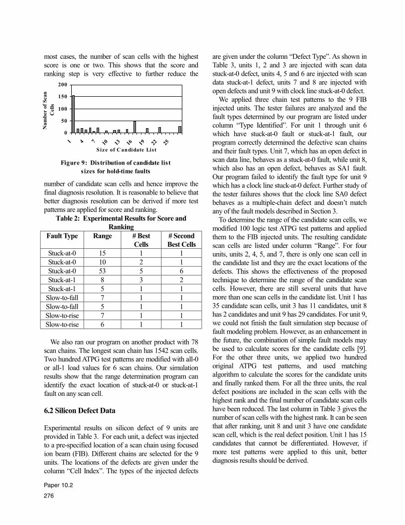
The typical distribution of candidate list sizes for hold-

time faults are shown in Figure 9. When comparing with

the candidate list sizes distribution for transition faults,

more scan cells have candidate lists consisting one scan

cell. Actually, for hold time faults, there are about 35%

of scan cells have a candidate list consisting of only one

scan cell. This result should be expected. The reason is

that even though the values of two consecutive scan cells

are required to determine an upper bound or lower

bound for hold time faults, this requirement is much

looser than those for transition faults because any value

transition (0 to 1 or 1 to 0) in the two consecutive scan

cells can be used to calculate the boundary of candidate

list for hold time faults. We also observed that some scan

cells have a large candidate list which tells us that further

improvement of the diagnostic resolution is necessary.

To improve the diagnostic resolution, we used the

matching algorithm to rank the candidate scan cells. In

this step, we used one hundred ATPG test patterns to

simulate each candidate scan cell. In this experiment, we

studied some cases where larger sizes of candidate lists

were obtained in the last step. The results are shown in

Table 2. The first column in Table 2 lists the fault types

of the targeting candidate lists. The sizes of the candidate

lists are shown in Column 2. Columns 3 and 4 show the

numbers of scan cells with the best score and the number

scan cells with the second best score. From Table 2, we

can see that after score and ranking, the number of

candidate scan cells can be reduced dramatically, and in

Figure 7: Distribution of candidate list

sizes for slow-to-fall faults

0

10

20

30

40

50

60

70

Size o f C andidate List

Figure 8: Distribution of candidate list

sizes for fast-to-rise faults

0

20

40

60

80

1 4 7 10 13 16 19 22 25 28

Size of Candidate List

Nu

mb

er o

f S

can

Cell

s

276

Paper 10.2

most cases, the number of scan cells with the highest

score is one or two. This shows that the score and

ranking step is very effective to further reduce the

number of candidate scan cells and hence improve the

final diagnosis resolution. It is reasonable to believe that

better diagnosis resolution can be derived if more test

patterns are applied for score and ranking.

Table 2: Experimental Results for Score and

Ranking

Fault Type Range # Best

Cells

# Second

Best Cells

Stuck-at-0 15 1 1

Stuck-at-0 10 2 1

Stuck-at-0 53 5 6

Stuck-at-1 8 3 2

Stuck-at-1 5 1 1

Slow-to-fall 7 1 1

Slow-to-fall 5 1 1

Slow-to-rise 7 1 1

Slow-to-rise 6 1 1

We also ran our program on another product with 78

scan chains. The longest scan chain has 1542 scan cells.

Two hundred ATPG test patterns are modified with all-0

or all-1 load values for 6 scan chains. Our simulation

results show that the range determination program can

identify the exact location of stuck-at-0 or stuck-at-1

fault on any scan cell.

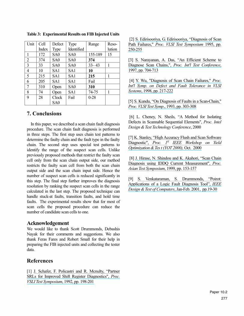
6.2 Silicon Defect Data

Experimental results on silicon defect of 9 units are

provided in Table 3. For each unit, a defect was injected

to a pre-specified location of a scan chain using focused

ion beam (FIB). Different chains are selected for the 9

units. The locations of the defects are given under the

column “Cell Index”. The types of the injected defects

are given under the column “Defect Type”. As shown in

Table 3, units 1, 2 and 3 are injected with scan data

stuck-at-0 defect, units 4, 5 and 6 are injected with scan

data stuck-at-1 defect, units 7 and 8 are injected with

open defects and unit 9 with clock line stuck-at-0 defect.

We applied three chain test patterns to the 9 FIB

injected units. The tester failures are analyzed and the

fault types determined by our program are listed under

column “Type Identified”. For unit 1 through unit 6

which have stuck-at-0 fault or stuck-at-1 fault, our

program correctly determined the defective scan chains

and their fault types. Unit 7, which has an open defect in

scan data line, behaves as a stuck-at-0 fault, while unit 8,

which also has an open defect, behaves as SA1 fault.

Our program failed to identify the fault type for unit 9

which has a clock line stuck-at-0 defect. Further study of

the tester failures shows that the clock line SA0 defect

behaves as a multiple-chain defect and doesn’t match

any of the fault models described in Section 3.

To determine the range of the candidate scan cells, we

modified 100 logic test ATPG test patterns and applied

them to the FIB injected units. The resulting candidate

scan cells are listed under column “Range”. For four

units, units 2, 4, 5, and 7, there is only one scan cell in

the candidate list and they are the exact locations of the

defects. This shows the effectiveness of the proposed

technique to determine the range of the candidate scan

cells. However, there are still several units that have

more than one scan cells in the candidate list. Unit 1 has

35 candidate scan cells, unit 3 has 11 candidates, unit 8

has 2 candidates and unit 9 has 29 candidates. For unit 9,

we could not finish the fault simulation step because of

fault modeling problem. However, as an enhancement in

the future, the combination of simple fault models may

be used to calculate scores for the candidate cells [9].

For the other three units, we applied two hundred

original ATPG test patterns, and used matching

algorithm to calculate the scores for the candidate units

and finally ranked them. For all the three units, the real

defect positions are included in the scan cells with the

highest rank and the final number of candidate scan cells

have been reduced. The last column in Table 3 gives the

number of scan cells with the highest rank. It can be seen

that after ranking, unit 8 and unit 3 have one candidate

scan cell, which is the real defect position. Unit 1 has 15

candidates that cannot be differentiated. However, if

more test patterns were applied to this unit, better

diagnosis results should be derived.

Figure 9: Distribution of candidate list

sizes for hold-time faults

0

50

100

150

200

1 4 7 10 13 16 19 22 25

S ize of C andidate List

Nu

mb

er o

f S

can

Cell

s

277

Paper 10.2

Table 3: Experimental Results on FIB Injected Units

Unit Cell

Index

Defect

Type

Type

Identified

Range Reso-

lution

1 172 SA0 SA0 155-189 15

2 374 SA0 SA0 374

3 33 SA0 SA0 33– 43 1

4 10 SA1 SA1 10

5 215 SA1 SA1 215 1

6 205 SA1 SA1 Fail

7 310 Open SA0 310

8 74 Open SA1 74-75 1

9 28 Clock

SA0

Fail 0-28

7. Conclusions

In this paper, we described a scan chain fault diagnosis

procedure. The scan chain fault diagnosis is performed

in three steps. The first step uses chain test patterns to

determine the faulty chain and the fault type in the faulty

chain. The second step uses special test patterns to

identify the range of the suspect scan cells. Unlike

previously proposed methods that restrict the faulty scan

cell only from the scan chain output side, our method

restricts the faulty scan cell from both the scan chain

output side and the scan chain input side. Hence the

number of suspect scan cells is reduced significantly in

this step. The final step further improves the diagnosis

resolution by ranking the suspect scan cells in the range

calculated in the last step. The proposed technique can

handle stuck-at faults, transition faults, and hold time

faults. The experimental results show that for most of

scan cells the proposed procedure can reduce the

number of candidate scan cells to one.

Acknowledgement We would like to thank Scott Drummonds, Debashis

Nayak for their comments and suggestions. We also

thank Feras Fares and Robert Small for their help in

preparing the FIB injected units and collecting the tester

data.

References

[1] J. Schafer, F. Policastri and R. Mcnulty, “Partner

SRLs for Improved Shift Register Diagnostics", Proc.

VSLI Test Symposium, 1992, pp. 198-201

[2] S. Edirisooriya, G. Edirisooriya, “Diagnosis of Scan

Path Failures," Proc. VLSI Test Symposium 1995, pp.

250-255

[3] S. Narayanan, A. Das, “An Efficient Scheme to

Diagnose Scan Chains,", Proc. Int'l Test Conference,

1997, pp. 704-713

[4] Y. Wu, "Diagnosis of Scan Chain Failures," Proc.

Int'l Symp. on Defect and Fault Tolerance in VLSI

Systems, 1998, pp. 217-222

[5] S. Kundu, “On Diagnosis of Faults in a Scan-Chain,"

Proc. VLSI Test Symp., 1993, pp. 303-308

[6] L. Cheney, N. Sheils, “A Method for Isolating

Defects in Scannable Sequential Elements", Proc. Intel

Design & Test Technology Conference, 2000

[7] K. Stanley, “High Accuracy Flush and Scan Software

Diagnostic", Proc. 1st IEEE Workshop on Yield

Optimization & Tes t (YOT 2000), Oct. 2000

[8] J. Hirase, N. Shindou and K. Akahori, “Scan Chain

Diagnosis using IDDQ Current Measurement", Proc.

Asian Test Symposium, 1999, pp. 153-157

[9] S. Venkataraman, S. Drummonds, “Poirot:

Applications of a Logic Fault Diagnosis Tool”, IEEE

Design & Test of Computers, Jan-Feb. 2001, pp.19-30