M4M 2009

A Tableau Method for Checking RuleAdmissibility in S4

Sergey Babenysheva, Vladimir Rybakova, Renate A. Schmidtb

and Dmitry Tishkovskyb

a Department of Computing and Mathematics,Manchester Metropolitan University, UK

b School of Computer Science,The University of Manchester, UK

Abstract

Rules that are admissible can be used in any derivations in any axiomatic system of a logic. In this paperwe introduce a method for checking the admissibility of rules in the modal logic S4. Our method is basedon a standard semantic ground tableau approach. In particular, we reduce rule admissibility in S4 tosatisfiability of a formula in a logic that extends S4. The extended logic is characterised by a class of modelsthat satisfy a variant of the co-cover property. The class of models can be formalised by a well-defined first-order specification. Using a recently introduced framework for synthesising tableau decision procedures thiscan be turned into a sound, complete and terminating tableau calculus for the extended logic, and gives atableau-based method for determining the admissibility of rules.

Keywords: Tableau calculus, admissible rule, modal logic, S4, tableau synthesis framework.

1 Introduction

Logical admissible rules were first considered by Lorenzen [12]. Initial investigationswere limited to observations on the existence of interesting examples of admissiblerules that are not derivable (see Harrop [7], Mints [13]). The area gained new mo-mentum when Friedman [2] posed the question whether algorithms exist for recog-nising whether rules in intuitionistic propositional logic IPC are admissible. Thisproblem and the corresponding problem for modal logic S4 are solved affirmativelyin Rybakov [15,17]. The same approach can be used for a broad range of proposi-tional modal logics, for example K4, S4, GL [18]. Roziere [14] presents a solution toFriedman’s problem for IPC that uses methods of proof theory.

The theory of admissible rules in S4 does not have the finite approximationproperty [11] in the strict sense. The algorithm in [15] is based on the existence ofa model (of bounded size) that witnesses the non-admissibility of a rule, but is notnecessarily a model for all the other admissible rules. In [1] it is observed that awitnessing model can be obtained by filtration.

This paper is electronically published inElectronic Notes in Theoretical Computer Science

URL: www.elsevier.com/locate/entcs

Babenyshev et al

Admissibility of rules has direct connections to the problem of unification. Arefined technique [18] is used for admissibility of rules with meta-variables, for uni-fication, for unification with parameters, and for the solvability of logical equationsin transitive modal logics.

Algorithms deciding admissibility for some transitive modal logics and IPC,based on projective formulae and unification, are described in Ghilardi [3,4,5,6].They combine resolution and tableau approaches for finding projective approxima-tions of a formula and rely on the existence of an algorithm for theorem proving. Apractically feasible realisation for S4 built on the algorithm for IPC in [5] is describedin [24]. These algorithms were specifically designed for finding general solutions formatching and unification problems. In contrast, the original algorithm of [15] canbe used to find only some solution of such problems in S4.

In this paper we focus on S4 and introduce a new method for recognising theadmissibility of rules. Our method is based on the reduction of the problem ofrule admissibility in S4 to the satisfiability of a certain formula in an extensionof S4. We refer to the extended logic as S4u,+. S4u,+ can be characterised by aclass of models, which satisfy a variant of the co-cover property that is definable bymodal formulae. This property is expressible in first-order logic and means that thesemantics of the logic can be formalised in first-order logic. We exploit this propertyin order to devise a tableau calculus for S4u,+ in a recently introduced frameworkfor automatically synthesising tableau calculi and decision procedures [21,22].

The tableau synthesis method of [22] works as follows.

(i) The user defines the formal semantics of the given logic in a many-sortedfirst-order language so that certain well-definedness conditions hold.

(ii) The method automatically reduces the semantic specification of the logic toSkolemised implicational forms which are then rewritten as tableau inferencerules. These are combined with some default closure and equality rules.

The set of rules obtained in this way provides a sound and constructively completecalculus. Furthermore, this set of rules automatically has a subformula propertywith respect to a finite subformula operator. If the logic can be shown to admitfinite filtration with respect to a well-defined first-order semantics then adding ageneral blocking mechanism produces a terminating tableau calculus [21].

We show how, using this method, a sound, complete and terminating tableaucalculus can be synthesised for the extended logic S4u,+. This tableau calculus isthen incorporated into a method for solving the rule admissibility problem in S4.

The paper is structured as follows. In Section 2 we define the syntax and seman-tics of the modal logic S4, and its extension S4u with the universal modality, in sucha way that they can be accommodated in the tableau synthesis framework of [22].The section also defines standard modal logic constructions and notions requiredfor the main results of the paper. In Section 3, we give definitions of derivableand admissible rules for S4 and state Rybakov’s criterion for testing admissibilityof rules in S4. The reduction of rule admissibility in S4 to satisfiability in S4u,+

is described in Section 4. In Section 5, we show how the formulaic variant of theco-cover property can be expressed by a set of first-order formulae that provide asuitable background theory for the specification of the semantics of S4u,+ in the

2

Babenyshev et al

Definitions of connectives Background theory

∀x(ν(¬p, x) ↔ ¬ν(p, x)

)∀x, y, z

(R(x, y) ∧R(y, z)→ R(x, z)

)∀x(ν(p ∨ q, x) ↔ ν(p, x) ∨ ν(q, x)

)∀x R(x, x)

∀x(ν(3p, x) ↔ ∃y (R(x, y) ∧ ν(p, y))

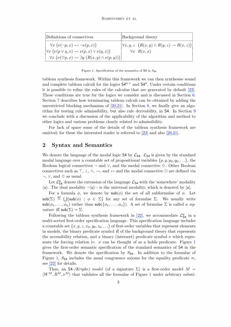
)Figure 1. Specification of the semantics of S4 in SS4

tableau synthesis framework. Within this framework we can then synthesise soundand complete tableau calculi for the logics S4u,+ and S4u. Under certain conditionsit is possible to refine the rules of the calculus that are generated by default [22].These conditions are true for the logics we consider and is discussed in Section 6.Section 7 describes how terminating tableau calculi can be obtained by adding theunrestricted blocking mechanism of [20,21]. In Section 8, we finally give an algo-rithm for testing rule admissibility, but also rule derivability, in S4. In Section 9we conclude with a discussion of the applicability of the algorithm and method toother logics and various problems closely related to admissibility.

For lack of space some of the details of the tableau synthesis framework areomitted; for these the interested reader is referred to [22] and also [20,21].

2 Syntax and Semantics

We denote the language of the modal logic S4 by LS4. LS4 is given by the standardmodal language over a countable set of propositional variables {p, q, p0, q0, . . .}, theBoolean logical connectives ¬ and ∨, and the modal connective 3. Other Booleanconnectives such as >, ⊥, ∧, →, and↔ and the modal connective 2 are defined via¬, ∨, and 3 as usual.

Let LuS4 denote the extension of the language LS4 with the ‘somewhere’ modality

〈u〉. The dual modality ¬〈u〉¬ is the universal modality, which is denoted by [u].For a formula φ, we denote by sub(φ) the set of all subformulae of φ. Let

sub(Σ) def=⋃{sub(φ) | φ ∈ Σ} for any set of formulae Σ. We usually write

sub(φ1, . . . , φn) rather than sub({φ1, . . . , φn}). A set of formulae Σ is called a sig-nature iff sub(Σ) = Σ.

Following the tableau synthesis framework in [22], we accommodate LuS4 in a

multi-sorted first-order specification language. This specification language includesa countable set {x, y, z, x0, y0, z0, . . .} of first-order variables that represent elementsin models, the binary predicate symbol R of the background theory that representsthe accessibility relation, and a binary (intersort) predicate symbol ν which repre-sents the forcing relation |=. ν can be thought of as a holds predicate. Figure 1gives the first-order semantic specification of the standard semantics of S4 in theframework. We denote the specification by SS4. In addition to the formulae ofFigure 1, SS4 includes the usual congruence axioms for the equality predicate ≈,see [22] for details.

Thus, an S4-(Kripke) model (of a signature Σ) is a first-order model M =〈WM , RM , νM 〉 that validates all the formulae of Figure 1 under arbitrary substi-

3

Babenyshev et al

tutions of LS4-formulae (from the signature Σ) for variables p and q.Let S4u be the extension of S4 with the somewhere (or universal) modality. The

semantic specification of S4u, denoted by SS4u , is the extension of the specificationSS4 of S4 with

∀x (ν(〈u〉p, x)↔ ∃y ν(p, y)).(1)

This defines the somewhere modality 〈u〉. An S4u-model (of a signature Σ) is bydefinition a first-order model M = 〈WM , RM , νM 〉 that validates this formula inaddition to all the formulae of Figure 1 under arbitrary substitutions of Lu

S4-formulae(from the signature Σ) for propositional variables p and q.

Note that if M is a model of the signature Σ then M is also a model of anysignature Σ′ ⊆ Σ. In the other direction, it is clear that every model M of a smallersignature Σ′ can be extended to a model of a bigger signature Σ by (re)defining theinterpretation of ν on formulae from Σ\Σ′ (by induction on their length). We oftenuse these facts when defining models.

A (Kripke) frame of S4 (resp. S4u) is a first-order structure F = 〈WF , RF 〉 thatvalidates all the formulae of the background theory of SS4 (resp. SS4u). A model Mis based on a frame F (or the underlying frame of M is F ) iff WM = WF andRM = RF .

A cluster of a model M is a set U ⊆WM such that for all w ∈WM and u ∈ Uit holds that (w, u), (u,w) ∈ RM iff w ∈ U . Any set of RM -incomparable clustersof M is called an anti-chain in M . A cluster U ⊆ WM is maximal iff (u,w) ∈ RMimplies w ∈ U for all w ∈WM and u ∈ U .

Let Σ be a fixed signature and M a model of the signature Σ. We say that aformula φ ∈ Σ is true (satisfied) in a world w ∈ WM (in symbols M,w |= φ) iff(φ,w) ∈ νM . A formula φ (from Σ) is valid in M (in symbols M |= φ) iff M,w |= φ

for every w ∈ WM . And, as usual, φ is satisfiable in M iff there is w ∈ WM suchthat M,w |= φ. A formula φ ∈ Σ is valid in a frame F (in symbols F |= φ) iff it istrue in every model M of the signature Σ based on F .

For a signature Σ and every element w of WM we define a Σ-type τΣ(w) of was the set of all formulae from Σ which are true in w, namely:

τΣ(w) def= {ψ ∈ Σ |M,w |= ψ}.

We omit the superscript Σ and write τ(w) if Σ is known from the context. A modelM of a signature Σ is called Σ-differentiated iff τΣ(w) = τΣ(v) implies w = v forall w, v ∈ WM . A model M is formulaic iff for every element w ∈ WM there is aformula φ such that M,w |= φ and M, v 6|= φ for all v ∈WM \ {w}. It is clear thatif Σ is finite then every Σ-differentiated model is also formulaic.

We call a Kripke model M of a signature Σ′ a definable variant of a model N ofa signature Σ if M and N are based on the same frame and for every propositionalvariable p ∈ Σ′ there is a formula φ ∈ Σ such that M,w |= p ⇐⇒ N,w |= φ forevery w ∈WM = WN .

Let Σ be the set of all formulae in n variables p1, . . . , pn. An S4-model M ofsignature Σ is called an n-characterising model for S4 iff M |= φ ⇐⇒ φ ∈ S4 forevery φ ∈ Σ.

4

Babenyshev et al

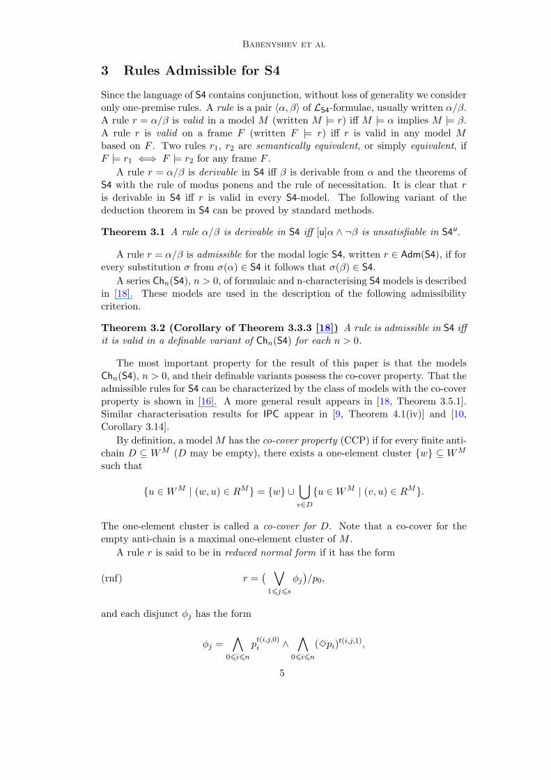
3 Rules Admissible for S4

Since the language of S4 contains conjunction, without loss of generality we consideronly one-premise rules. A rule is a pair 〈α, β〉 of LS4-formulae, usually written α/β.A rule r = α/β is valid in a model M (written M |= r) iff M |= α implies M |= β.A rule r is valid on a frame F (written F |= r) iff r is valid in any model Mbased on F . Two rules r1, r2 are semantically equivalent, or simply equivalent, ifF |= r1 ⇐⇒ F |= r2 for any frame F .

A rule r = α/β is derivable in S4 iff β is derivable from α and the theorems ofS4 with the rule of modus ponens and the rule of necessitation. It is clear that ris derivable in S4 iff r is valid in every S4-model. The following variant of thededuction theorem in S4 can be proved by standard methods.

Theorem 3.1 A rule α/β is derivable in S4 iff [u]α ∧ ¬β is unsatisfiable in S4u.

A rule r = α/β is admissible for the modal logic S4, written r ∈ Adm(S4), if forevery substitution σ from σ(α) ∈ S4 it follows that σ(β) ∈ S4.

A series Chn(S4), n > 0, of formulaic and n-characterising S4 models is describedin [18]. These models are used in the description of the following admissibilitycriterion.

Theorem 3.2 (Corollary of Theorem 3.3.3 [18]) A rule is admissible in S4 iffit is valid in a definable variant of Chn(S4) for each n > 0.

The most important property for the result of this paper is that the modelsChn(S4), n > 0, and their definable variants possess the co-cover property. That theadmissible rules for S4 can be characterized by the class of models with the co-coverproperty is shown in [16]. A more general result appears in [18, Theorem 3.5.1].Similar characterisation results for IPC appear in [9, Theorem 4.1(iv)] and [10,Corollary 3.14].

By definition, a model M has the co-cover property (CCP) if for every finite anti-chain D ⊆ WM (D may be empty), there exists a one-element cluster {w} ⊆ WM

such that

{u ∈WM | (w, u) ∈ RM} = {w} ∪⋃v∈D{u ∈WM | (v, u) ∈ RM}.

The one-element cluster is called a co-cover for D. Note that a co-cover for theempty anti-chain is a maximal one-element cluster of M .

A rule r is said to be in reduced normal form if it has the form

(rnf) r =( ∨

16j6s

φj)/p0,

and each disjunct φj has the form

φj =∧

06i6n

pt(i,j,0)i ∧

∧06i6n

(3pi)t(i,j,1),

5

Babenyshev et al

where (i) all φj are different, (ii) p0, . . . , pn denote propositional variables, (iii) t is aBoolean function t : {0, . . . , n}×{1, . . . , s}×{0, 1} → {0, 1} (i.e., t(i, j, z) ∈ {0, 1}),and (iv) α0 def= ¬α and α1 def= α for any formula α.

Using the renaming technique any modal rule can be transformed into an equiv-alent rule in reduced normal form [15].

Lemma 3.3 Every rule r = α/β can be transformed in exponential time to a de-finably equivalent rule rnf(r) in the reduced normal form.

Proof We shall specify the general algorithm described in [18, Lemma 3.1.3] and[18, Theorem 3.1.11].

Let r = α/β be an inference rule. Denote sub(α, β) as sub(r), and let V ar(r) bethe set of propositional variables occurring in r. We will need a set of new variablesZ = {zγ | γ ∈ sub(r)}. Let us consider the rule in the intermediate form:

rif = zα ∧∧

γ∈sub(r)\V ar(r)

(zγ ↔ γ])/zβ,

where

γ] =

{zδ ∨ zε when γ = δ ∨ ε,∗zδ when γ = ∗δ for ∗ ∈ {¬,3}.

The rules r and rif are equivalent. Indeed, suppose M is a model with a valuationν := νM : V ar(r) → 2W over the frame F := 〈W,R〉 = FM , such that M 6|= r.Then F |=ν α(x) and there exists an element w ∈ W , such that F,w 6|=ν β(x). Letµ : Z → 2W be the valuation defined as follows: µ(zγ) = ν(γ). It is straightforwardto show that F |=µ zα ∧

∧γ∈sub(r)\V ar(r)(zγ ↔ γ]). In addition, F,w 6|=µ zβ.

For the other direction, suppose F |=µ zα ∧∧{zγ ↔ γ] | γ ∈ sub(r) \ V ar(r)}

and F,w 6|=µ zβ, for some valuation µ : Z → 2W and some w ∈ W . Defineν : V ar(r) → 2W by ν(xi) = µ(zxi). It follows directly that for all γ ∈ sub(r),ν(γ) = µ(zγ). Thus F |=ν α(x), F,w 6|=µ β(x), hence F 6|=ν r.

Finally, we transform the premise of the obtained rule rif into a perfect disjunc-tive normal form over primitives of the form xi and 3xi. This requires no more thanexponential time on the number of variables, i.e., on the number of subformulas ofthe original rule (the same as for reduction of any boolean formula to the perfectdisjunctive normal form). 2

Lemma 3.3 gives us a procedure, that deterministically assigns a particular nor-mal form to each rule. We will denote this form by by rnf(r). As seen from theproof of Lemma 3.3, the variables in the reduced form represent the subformulas ofα and β. In particular, the variable xβ (in the future x1) stands for the conclusionβ itself. Note that Lemma 3.3 proves more than the equivalence of r and rnf(r).Indeed, it follows from the proof that if r is refutable in a model N then rnf(r) isrefutable in a definable variant M of N with M,w |= qγ ⇐⇒ N,w |= γ for allγ ∈ sub(r).

Let r be any rule in reduced normal form (rnf). Let Θ(r) def= {φ1, . . . , φs} be theset of all disjuncts of r. For every φj ∈ Θ(r), let

θ(φj)def= {pi | t(i, j, 0) = 1} and θ3(φj)

def= {pi | t(i, j, 1) = 1}.

6

Babenyshev et al

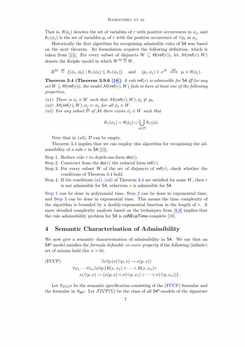
That is, θ(φj) denotes the set of variables of r with positive occurrences in φj , andθ3(φj) is the set of variables pi of r with the positive occurrence of 3pi in φj .

Historically the first algorithm for recognising admissible rules of S4 was basedon the next theorem. Its formulation requires the following definition, which istaken from [15]. For every subset of disjuncts W ⊆ Θ(rnf(r)), let M(rnf(r),W )denote the Kripke model in which WM def= W ,

RMdef= {(φ1, φ2) | θ3(φ2) ⊆ θ3(φ1)} and (pi, φj) ∈ νM

def⇐⇒ pi ∈ θ(φj).

Theorem 3.4 (Theorem 3.9.6 [18]) A rule rnf(r) is admissible for S4 iff for anyset W ⊆ Θ(rnf(r)), the modelM(rnf(r),W ) fails to have at least one of the followingproperties.

(a1) There is φj ∈W such that M(rnf(r),W ), φj 6|= p0.(a2) M(rnf(r),W ), φj |= φj for all φj ∈W .(a3) For any subset D of M there exists φj ∈W such that

θ3(φj) = θ(φj) ∪⋃φ∈D

θ3(φ).

Note that in (a3), D can be empty.Theorem 3.4 implies that we can employ this algorithm for recognising the ad-

missibility of a rule r in S4 [15].

Step 1. Reduce rule r to depth-one-form do(r).Step 2. Construct from the do(r) the reduced form rnf(r).Step 3. For every subset W of the set of disjuncts of rnf(r), check whether the

conditions of Theorem 3.4 hold.Step 4. If the conditions (a1)–(a3) of Theorem 3.4 are satisfied for some W , then r

is not admissible for S4, otherwise r is admissible for S4.

Step 1 can be done in polynomial time, Step 2 can be done in exponential time,and Step 3 can be done in exponential time. This means the time complexity ofthe algorithm is bounded by a doubly-exponential function in the length of r. Amore detailed complexity analysis based on the techniques from [8,9] implies thatthe rule admissibility problem for S4 is coNExpTime-complete [10].

4 Semantic Characterisation of Admissibility

We now give a semantic characterisation of admissibility in S4. We say that anS4u-model satisfies the formula definable co-cover property if the following (infinite)set of axioms hold (for n > 0):

∃x∀p (ν(3p, x)→ ν(p, x))(FCCP)

∀x1 · · · ∀xn∃x∀p(R(x, x1) ∧ · · · ∧R(x, xn)∧

ν(3p, x)→ (ν(p, x) ∨ ν(3p, x1) ∨ · · · ∨ ν(3p, xn))).

Let SFCCP be the semantic specification consisting of the (FCCP) formulae andthe formulae in SS4u . Let FCCP(Σ) be the class of all S4u-models of the signature

7

Babenyshev et al

Σ that satisfy all instances of the formulae of SFCCP under substitutions of LuS4-

formulae in Σ for propositional variables.Let S4u,+ be the modal logic with the language Lu

S4 that has SFCCP as semanticspecification. The following theorem is a direct consequence of the definitions aboveand the fact that all n-characterising models Chn(S4) for S4 satisfy the (FCCP)formulae.

Theorem 4.1 S4u,+ is a conservative extension of S4.

Now we prove that S4u,+ has the effective finite model property. Let Σ be afixed signature and M an S4u,+-model of the signature Σ. We define the filtrated(through Σ) model M as follows. The equivalence ∼ on the set WM is defined byw ∼ v

def⇐⇒ τ(w) = τ(v). Further, [w] def= {v ∈ WM | w ∼ v} and WM def= {[w] | w ∈WM}. Next, RM def= {([w], [v]) | M,v |= ψ implies M,w |= 3ψ for every 3ψ ∈ Σ}and, finally, νM def= {(ψ, [w]) | (ψ,w) ∈ νM} for every ψ ∈ Σ.

The following lemma can be proved by induction on the structure of formulaein Σ by verifying that all semantic conditions in SFCCP hold.

Lemma 4.2 (Filtration Lemma) M is an S4u,+-model of the signature Σ.

Note that by definition M is Σ-differentiated and it is finite whenever Σ is finite.

Theorem 4.3 (The Effective Finite Model Property) Let φ be a formulaand n the length of φ (i.e., the number of symbols in φ). If φ is satisfiable inan S4u,+-model (of the signature sub(φ)) then it is satisfiable in a finite S4u,+-model(of the signature sub(φ)) and its size does not exceed 2n.

Theorem 4.4 α/β ∈ Adm(S4) iff [u]α ∧ ¬β is unsatisfiable in S4u,+.

Proof Suppose α/β is not admissible and p1, . . . , pn are all the propositional vari-ables occurring in α and β. Then there is a model M—a definable variant ofChn(S4) such that M 6|= α/β. This model has the co-cover property and it isroutine to transform M into an S4u,+-model satisfying [u]α ∧ ¬β.

For the converse, let Σ def= sub([u]α∧¬β) and suppose [u]α∧¬β is satisfiable in anS4u,+-model. Then it is satisfiable in a finite Σ-differentiated S4u,+-model M (of thesignature Σ), by the Filtration Lemma. Let sub3(α, β) def= {3γ | γ ∈ sub(α, β)} ∪sub(α, β) for any LS4-formulae α and β. For every w ∈ WM let τ3(w) def= {γ ∈sub3(α, β) |M,w |= γ} and

φ(w) def=∧

γ∈sub(α,β)

qχ(γ)γ ∧

∧γ∈sub(α,β)

3qχ(3γ)γ ,

where χ is the characteristic function of the set τ3(w). Let us consider the modelM∗

def= 〈WM∗ , RM∗, νM

∗〉, where WM∗ def= {φ(w) | w ∈ WM}, (φ(u), φ(v)) ∈RM

∗ def⇐⇒ (u, v) ∈ RM , and (qγ , φ(w)) ∈ νM∗ def⇐⇒ M,w |= γ. Each φ(w) is a

disjunct in reduced normal form rnf(r). Therefore we have that

• WM∗ ⊆ Θ(rnf(r)),• 〈WM∗ , RM

∗〉 is isomorphic to the underlying frame of M ,

8

Babenyshev et al

• M∗ satisfies conditions (a1)–(a3) of Theorem 3.4.

By Theorem 3.4, rnf(r) is not admissible, and hence neither is r. 2

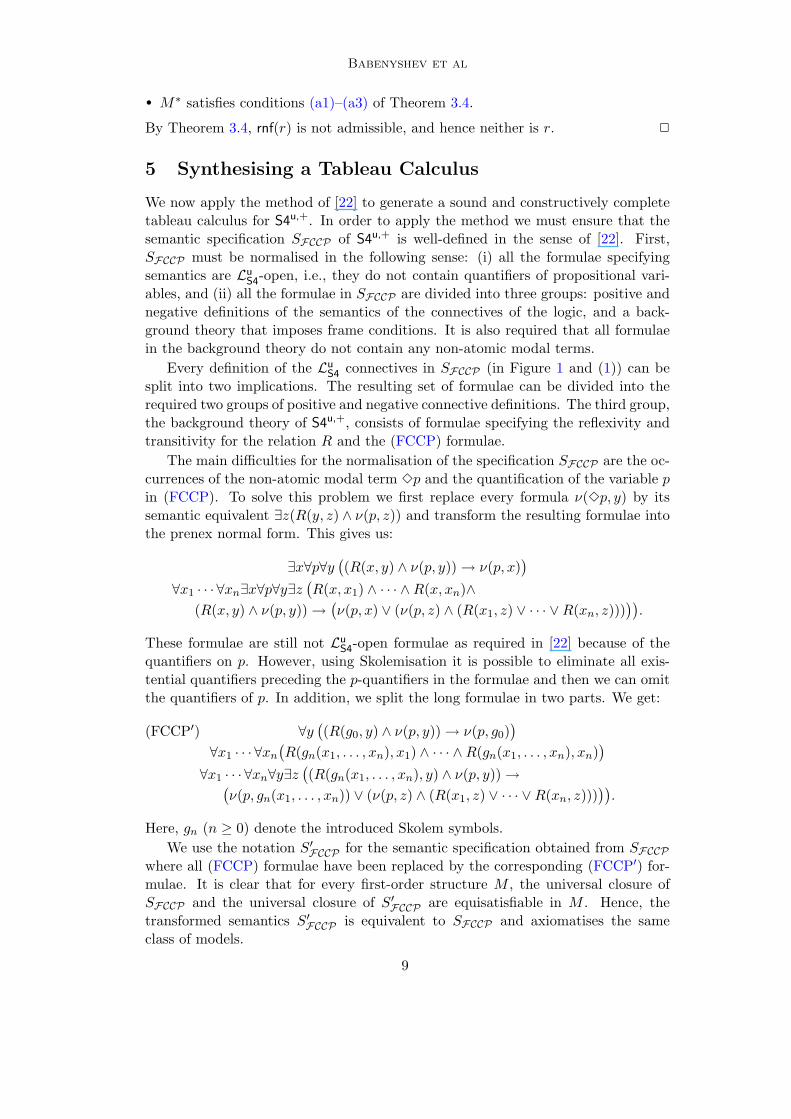
5 Synthesising a Tableau Calculus

We now apply the method of [22] to generate a sound and constructively completetableau calculus for S4u,+. In order to apply the method we must ensure that thesemantic specification SFCCP of S4u,+ is well-defined in the sense of [22]. First,SFCCP must be normalised in the following sense: (i) all the formulae specifyingsemantics are Lu

S4-open, i.e., they do not contain quantifiers of propositional vari-ables, and (ii) all the formulae in SFCCP are divided into three groups: positive andnegative definitions of the semantics of the connectives of the logic, and a back-ground theory that imposes frame conditions. It is also required that all formulaein the background theory do not contain any non-atomic modal terms.

Every definition of the LuS4 connectives in SFCCP (in Figure 1 and (1)) can be

split into two implications. The resulting set of formulae can be divided into therequired two groups of positive and negative connective definitions. The third group,the background theory of S4u,+, consists of formulae specifying the reflexivity andtransitivity for the relation R and the (FCCP) formulae.

The main difficulties for the normalisation of the specification SFCCP are the oc-currences of the non-atomic modal term 3p and the quantification of the variable pin (FCCP). To solve this problem we first replace every formula ν(3p, y) by itssemantic equivalent ∃z(R(y, z) ∧ ν(p, z)) and transform the resulting formulae intothe prenex normal form. This gives us:

∃x∀p∀y((R(x, y) ∧ ν(p, y))→ ν(p, x)

)∀x1 · · · ∀xn∃x∀p∀y∃z

(R(x, x1) ∧ · · · ∧R(x, xn)∧

(R(x, y) ∧ ν(p, y))→(ν(p, x) ∨ (ν(p, z) ∧ (R(x1, z) ∨ · · · ∨R(xn, z)))

)).

These formulae are still not LuS4-open formulae as required in [22] because of the

quantifiers on p. However, using Skolemisation it is possible to eliminate all exis-tential quantifiers preceding the p-quantifiers in the formulae and then we can omitthe quantifiers of p. In addition, we split the long formulae in two parts. We get:

∀y((R(g0, y) ∧ ν(p, y))→ ν(p, g0)

)(FCCP′)

∀x1 · · · ∀xn(R(gn(x1, . . . , xn), x1) ∧ · · · ∧R(gn(x1, . . . , xn), xn)

)∀x1 · · · ∀xn∀y∃z

((R(gn(x1, . . . , xn), y) ∧ ν(p, y))→(

ν(p, gn(x1, . . . , xn)) ∨ (ν(p, z) ∧ (R(x1, z) ∨ · · · ∨R(xn, z))))).

Here, gn (n ≥ 0) denote the introduced Skolem symbols.We use the notation S′FCCP for the semantic specification obtained from SFCCP

where all (FCCP) formulae have been replaced by the corresponding (FCCP′) for-mulae. It is clear that for every first-order structure M , the universal closure ofSFCCP and the universal closure of S′FCCP are equisatisfiable in M . Hence, thetransformed semantics S′FCCP is equivalent to SFCCP and axiomatises the sameclass of models.

9

Babenyshev et al

Decomposition tableau rules:

ν(¬p, x)

¬ν(p, x)

¬ν(¬p, x)

ν(p, x)ν(p ∨ q, x)

ν(p, x) | ν(q, x)

¬ν(p ∨ q, x)

¬ν(p, x), ¬ν(q, x)ν(3p, x)

R(x, f3(p, x)), ν(p, f3(p, x))

ν(¬3p, x)

¬R(x, y) | ¬ν(p, y)

ν(〈u〉p, x)

ν(p, fu(p))

ν(¬〈u〉p, x), y ≈ y¬ν(p, y)

Theory tableau rules:

x ≈ xR(x, x)

x ≈ x, y ≈ y, z ≈ z¬R(x, y) | ¬R(y, z) | R(x, z)

Infinite set of (FCCP) tableau rules (n > 0):

(cc0):p ≈ p, y ≈ y

¬R(g0, y) | ¬ν(p, y) | ν(p, g0)(ccn

0 ):x1 ≈ x1, . . . , xn ≈ xn, y ≈ yR(gn(x), x1), . . . , R(gn(x), xn)

(ccn1 ):

p ≈ p, x1 ≈ x1, . . . , xn ≈ xn, y ≈ y¬R(gn(x), y) | ¬ν(p, y) | ν(p, gn(x)) | R(x1, hn(p, x, y)), ν(p, hn(p, x, y)) | · · ·

Closure tableau rules:

ν1(p, x), ¬ν1(p, x)

⊥R(x, y), ¬R(x, y)

⊥

Figure 2. Generated tableau rules for S4u,+

R(x, y)

x ≈ x, y ≈ y¬R(x, y)

x ≈ x, y ≈ y¬ν(p, x)

p ≈ p, x ≈ xν(p, x)

p ≈ p, x ≈ xR(x, y), x ≈ z

R(z, y)

R(x, y), y ≈ zR(x, z)

ν(p, x), x ≈ yν(p, y)

x ≈ yy ≈ x

x ≈ y, y ≈ zx ≈ z

Figure 3. Equality congruence rules for predicates occurring in SS4u .

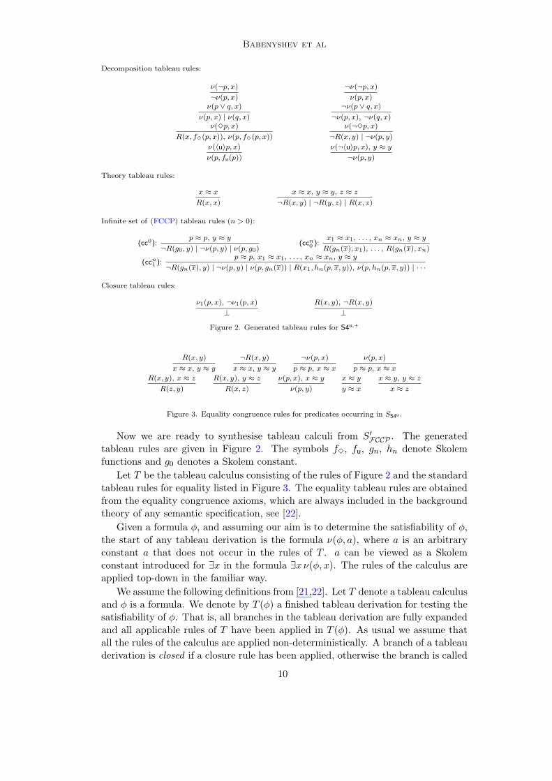
Now we are ready to synthesise tableau calculi from S′FCCP . The generatedtableau rules are given in Figure 2. The symbols f3, fu, gn, hn denote Skolemfunctions and g0 denotes a Skolem constant.

Let T be the tableau calculus consisting of the rules of Figure 2 and the standardtableau rules for equality listed in Figure 3. The equality tableau rules are obtainedfrom the equality congruence axioms, which are always included in the backgroundtheory of any semantic specification, see [22].

Given a formula φ, and assuming our aim is to determine the satisfiability of φ,the start of any tableau derivation is the formula ν(φ, a), where a is an arbitraryconstant a that does not occur in the rules of T . a can be viewed as a Skolemconstant introduced for ∃x in the formula ∃x ν(φ, x). The rules of the calculus areapplied top-down in the familiar way.

We assume the following definitions from [21,22]. Let T denote a tableau calculusand φ is a formula. We denote by T (φ) a finished tableau derivation for testing thesatisfiability of φ. That is, all branches in the tableau derivation are fully expandedand all applicable rules of T have been applied in T (φ). As usual we assume thatall the rules of the calculus are applied non-deterministically. A branch of a tableauderivation is closed if a closure rule has been applied, otherwise the branch is called

10

Babenyshev et al

open. The tableau derivation T (φ) is closed if all its branches are closed and T (φ)is open otherwise. A calculus T is sound (for a logic L) iff for any formula φ, eachT (φ) is open whenever φ is satisfiable in an L-model. T is complete iff for anyunsatisfiable formula φ there is a T (φ) which is closed. T is constructively complete(for L) iff for any open branch in a finished tableau derivation in T it is possible toconstruct an L-model from terms of the branch such that the model reflects all theformulae occurring in the branch. (Constructive completeness is a stronger notionthan completeness.) T is said to be terminating if every finished open tableauderivation in T has a finite open branch.

It is easy to check that the specification S′FCCP for S4u,+ is well-defined in thesense of [22]. A consequence of [22, Theorems 1 and 2] is this result.

Theorem 5.1 T is a sound and constructively complete calculus for S4u,+.

6 A Refined Tableau Calculus

The generated calculus T can be refined as follows. First, it is possible to refinethe calculus by moving negated conclusions in certain rules up to premise positions.We move formulae that contain only propositional variables and do not contain anycomplex modal terms upwards. It is not difficult to check for each rule that thecondition given in [22, Theorem 3] for this refinement to preserve soundness andconstructive completeness is true.

Second, we can apply the second refinement described in [22, Section 5]. For thiswe extend the language Lu

S4 by introducing a countable set {i, j, k, . . .} of nominalvariables and logical connectives (acting on nominals) which correspond to Skolemfunctions and constants. The @ operator can be introduced and specified in such away that @iφ

def= [u](i→ φ) for every nominal term i and formula φ (of the extendedlanguage). It is not difficult to see that the semantics of all the connectives of theextended language can be represented in the language itself (see [22, Section 5]).

Summing up, the refined rules we obtain are given in Figure 4. In these rules,i, j, k, i1, . . . , in denote nominal variables, and f3, fu, gn, and hn (n ≥ 0) denote‘nominal functions’ which correspond to the Skolem functions with same names.

Let T+ be the tableau calculus which consists of the rules of Figure 4 and therefined equality rules given in Figure 5. In T+, a tableau derivation for testing thesatisfiability of φ starts with a formula @i0φ where i0 is a fresh nominal constant.

Theorem 6.1 T+ is a sound and constructively complete tableau calculus for S4u,+.

7 A Terminating Tableau Calculus

Our proof of Theorem 4.3 that S4u,+ has the effective finite model property uses afiltration argument. That is, in the terminology of [21], S4u,+ admits finite filtration.Using the results of [21], this means that the tableau calculi generated in Section 5and 6 can be turned into terminating tableau calculi. In particular, we are interestedonly in the refined calculus T+.

Adding the following unrestricted blocking rule to T+ gives a terminating tableau

11

Babenyshev et al

Decomposition tableau rules:

(¬):@i¬¬p

@ip

(∨):@i(p ∨ q)@ip | @iq

(¬∨):@i¬(p ∨ q)@i¬p, @i¬q

(3):@i3p

@i3f3(p, i), @f3(p,i)p(¬3):

@i¬3p, @i3j

@j¬p

(〈u〉):@i〈u〉p@fu(p)p

(¬〈u〉):@i¬〈u〉p, @jj

@j¬p

Theory tableau rules:

(refl):@ii

@i3i(trans):

@i3j, @j3k

@i3k

Infinite set of (FCCP′) tableau rules (n > 0):

(cc′00):@g0g0

(cc′01):@g03i, @ip

@g0p

(cc′n0 ):@i1 i1, . . . , @in in

@gn(i)3i1, . . . , @gn(i)3in

(cc′n1 ):@gn(i)3j, @jp

@gn(i)p | @i13hn(p, i, j), @hn(p,i,j)p | · · · | @in3hn(p, i, j), @hn(p,i,j)p

Closure tableau rules:

(⊥):@ip, @i¬p⊥

Figure 4. Refined tableau rules for S4u,+

(refl≈):@ip

@ii(sym≈):

@ij

@ji(trans≈):

@ij, @jk

@ik

(con≈0):@ip, @ij

@jp(con≈1):

@i3j, @jk

@i3k

Figure 5. Refined equality congruence rules

calculus.(ub):

@ii, @jj

@ij | @i¬jThe conditions that blocking must satisfy are:

(b1) The rules (3) and (〈u〉) are never applied to formulae of the form @i3j and,respectively, @i〈u〉j where j is a nominal term.

(b2) If @ij appears in a branch and i < j (i.e., nominal i appeared strictly earlierthan nominal j in the derivation) then all further applications of the tableaurules which produce new nominals (in our case the (3), (〈u〉), (cc′00) and (cc′n0 )rules) to the formulae with occurrences of j are not performed within thebranch.

(b3) In every open branch there is some node from which point onwards beforeany application of any tableau rule that produces new nominals (i.e., the (3),(〈u〉), (cc′00) and (cc′n0 ) rules) all possible applications of the (ub) rule havebeen performed.

We denote the extended calculus by TS4u,+ .

12

Babenyshev et al

Since T+ is sound and constructively complete for S4u,+, and S4u,+ admits finitefiltration the results in [20] allow us to state:

Theorem 7.1 TS4u,+ is a sound, (constructively) complete and terminating tableaucalculus for S4u,+.

Let TS4u be the tableau calculus which consists of the same set of rules as TS4u,+

but excludes the (FCCP′) rules: (cc′00), (cc′01), (cc′n0 ), and (cc′n1 ). Applying tableausynthesis to S4u in a similar way gives the following result.

Theorem 7.2 TS4u is a sound, (constructively) complete and terminating tableaucalculus for S4u.

8 A Tableau Method for Testing Rule Admissibility

Putting all the results together (in particular Theorems 3.1, 4.4, 7.1 and 7.2) hereis a method for determining whether a modal rule is admissible in S4, or not.

Step 1. Given an S4-rule α/β, rewrite it to [u]α ∧ ¬β.Step 2. Use the tableau calculus TS4u to test the satisfiability of [u]α ∧ ¬β in S4u.Step 3. If TS4u([u]α ∧ ¬β) is closed, i.e., [u]α ∧ ¬β is unsatisfiable in S4u, then stop

and return ‘derivable’.Step 4. Otherwise (i.e., TS4u([u]α ∧ ¬β) is open), continue the tableau derivation

with the rules in TS4u plus the rules (cc′00), (cc′01), (cc′n0 ), and (cc′n1 ). Inparticular, continue the derivation with a finite open branch of TS4u([u]α ∧¬β) using the rules of TS4u,+ until the derivation stops.

Step 5. If TS4u,+([u]α ∧ ¬β) is closed then return ‘not derivable and admissible’.Otherwise, i.e., if TS4u,+([u]α ∧ ¬β) is open, return ‘not admissible’.

The answers returned by the method are either ‘derivable’, ‘not derivable andadmissible’, or ‘not admissible’. If a rule is derivable it is also admissible but notconversely.

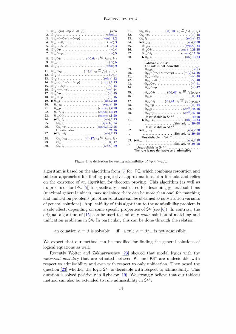
Figure 6 demonstrates the algorithm for the rule 3p ∧ 3¬p/⊥. The Step 1rewrites the rule to ¬〈u〉(¬3p ∨ ¬3¬p) modulo standard modal equivalences. Theblack triangles in the figure denote branching points in the derivation. A branchexpansion after a branching point is indicated by appropriate indentation.

9 Concluding Remarks

A major difficulty in dealing with S4-admissibility, is that the theory of S4-ad-missible rules does not have the finite approximation property [11] in this sense:for a rule r /∈ Adm(S4), there is no single finite Kripke model M separating r

from Adm(S4), (i.e., such that M |= Adm(S4), but M 6|= r). Therefore the tableaualgorithm that we have introduced in this paper builds open branches that representa (possibly) infinite Adm(S4)-model and is a counter-model to a non-admissiblerule. The subsequent filtration provides a finite model (not necessarily an Adm(S4)-model) witnessing the refutation.

A known algorithm that can handle S4-admissibility appears in Zucchelli [24]and is based on the research of Ghilardi [3,4,5,6] on projective approximations. This

13

Babenyshev et al

1. @i0¬〈u〉(¬3p ∨ ¬3¬p) . . . . . . . . . . . . . . . . given2. @i0 i0 . . . . . . . . . . . . . . . . . . . . . . . . . . . . . . (refl≈),13. @i0¬(¬3p ∨ ¬3¬p) . . . . . . . . . . . . . . .(¬〈u〉),1,24. @i0¬¬3p . . . . . . . . . . . . . . . . . . . . . . . . . . . . (¬∨),35. @i0¬¬3¬p . . . . . . . . . . . . . . . . . . . . . . . . . . (¬∨),36. @i03p . . . . . . . . . . . . . . . . . . . . . . . . . . . . . . . . (¬),47. @i03¬p . . . . . . . . . . . . . . . . . . . . . . . . . . . . . . . (¬),5

8. @i03i1 . . . . . . . . . . . . . . . . (3),6: i1def= f3(p, i0)

9. @i1p . . . . . . . . . . . . . . . . . . . . . . . . . . . . . . . . . . (3),610. @i1 i1 . . . . . . . . . . . . . . . . . . . . . . . . . . . . . . (refl≈),9

11. @i03i2 . . . . . . . . . . . . . . .(3),7: i2def= f3(¬p, i0)

12. @i2¬p . . . . . . . . . . . . . . . . . . . . . . . . . . . . . . . . (3),713. @i2 i2 . . . . . . . . . . . . . . . . . . . . . . . . . . . . . (refl≈),1214. @i2¬(¬3p ∨ ¬3¬p) . . . . . . . . . . . . . (¬〈u〉),1,1315. @i2¬¬3p . . . . . . . . . . . . . . . . . . . . . . . . . . . (¬∨),1416. @i2¬¬3¬p . . . . . . . . . . . . . . . . . . . . . . . . . (¬∨),1417. @i23p . . . . . . . . . . . . . . . . . . . . . . . . . . . . . . . (¬),1518. @i23¬p . . . . . . . . . . . . . . . . . . . . . . . . . . . . . . (¬),1619. I@i0 i1 . . . . . . . . . . . . . . . . . . . . . . . . . . . . (ub),2,1020. @i1 i0 . . . . . . . . . . . . . . . . . . . . . . . . . . (sym≈),1921. @i0p . . . . . . . . . . . . . . . . . . . . . . . . . (con≈0),9,2022. @i13i1 . . . . . . . . . . . . . . . . . . . . . . (con≈0),8,1923. @i03i0 . . . . . . . . . . . . . . . . . . . . . . (con≈1),8,2024. I@i0 i2 . . . . . . . . . . . . . . . . . . . . . . . . . . (ub),2,1325. @i2 i0 . . . . . . . . . . . . . . . . . . . . . . . . .(sym≈),2426. @i0¬p . . . . . . . . . . . . . . . . . . . . (con≈0),12,25

Unsatisfiable . . . . . . . . . . . . . . . . . . . . . . . 21,2627. I@i0¬i2 . . . . . . . . . . . . . . . . . . . . . . . . (ub),2,13

28. @i23i3 . . . . . . . . . . . (3),17: i3def= f3(p, i2)

29. @i3p . . . . . . . . . . . . . . . . . . . . . . . . . . . . . (3),1730. @i3 i3 . . . . . . . . . . . . . . . . . . . . . . . . . (refl≈),29

31. @i23i4 . . . . . . . . . . (3),18: i4def= f3(¬p, i2)

32. @i4¬p . . . . . . . . . . . . . . . . . . . . . . . . . . . . (3),1833. @i4 i4 . . . . . . . . . . . . . . . . . . . . . . . . . (refl≈),3234. I@i0 i3 . . . . . . . . . . . . . . . . . . . . . . . . (ub),2,3035. @i3 i0 . . . . . . . . . . . . . . . . . . . . . . . (sym≈),3436. @i23i0 . . . . . . . . . . . . . . . . . .(con≈1),28,3537. @i23i2 . . . . . . . . . . . . . . . . . . . (trans),11,3638. I@i2 i4 . . . . . . . . . . . . . . . . . . . . . (ub),13,33. . . . . . . . . . . . . . . . . . . . . . . . . . . . . . . . . . . . . . . .

Satisfiable in S4u . . . . . . . . . . . . . . . . . . . . .The rule is not derivable . . . . . . . . . . . . .

39. @g0g0 . . . . . . . . . . . . . . . . . . . . . . . . . (cc′00)40. @g0¬(¬3p ∨ ¬3¬p) . . . . . . (¬〈u〉),1,3541. @g0¬¬3p . . . . . . . . . . . . . . . . . . . (¬∨),4042. @g0¬¬3¬p . . . . . . . . . . . . . . . . . . (¬∨),4043. @g03p . . . . . . . . . . . . . . . . . . . . . . . . (¬),4144. @g03¬p . . . . . . . . . . . . . . . . . . . . . . (¬),42

45. @g03i5 . . . . . . . (3),43: i5def= f3(p, g0)

46. @i5p . . . . . . . . . . . . . . . . . . . . . . . . . . (3),43

47. @g03i6 . . . . . . (3),44: i6def= f3(¬p, g0)

48. @i6¬p . . . . . . . . . . . . . . . . . . . . . . . . (3),4449. @g0p . . . . . . . . . . . . . . . . . . . . (cc′01),45,46

50. @g0¬p . . . . . . . . . . . . . . . . . . . (cc′01),47,48

Unsatisfiable in S4u,+ . . . . . . . . . . . 49,5051. I@i2¬i4 . . . . . . . . . . . . . . . . . . . . (ub),13,33. . . . . . . . . . . . . . . . . . . . . . . Similarly to 39–50

Unsatisfiable in S4u,+ . . . . . . . . . . . . . . . . .52. I@i0¬i3 . . . . . . . . . . . . . . . . . . . . . . . (ub),2,30. . . . . . . . . . . . . . . . . . . . . . . . Similarly to 39–50

Unsatisfiable in S4u,+ . . . . . . . . . . . . . . . . . .53. I@i0¬i1 . . . . . . . . . . . . . . . . . . . . . . . . . . (ub),2,10. . . . . . . . . . . . . . . . . . . . . . . . . . . . Similarly to 39–50

Unsatisfiable in S4u,+ . . . . . . . . . . . . . . . . . . . . . .The rule is not derivable and admissible

Figure 6. A derivation for testing admissibility of 3p ∧3¬p/⊥.

algorithm is based on the algorithm from [5] for IPC, which combines resolution andtableau approaches for finding projective approximations of a formula and relieson the existence of an algorithm for theorem proving. This algorithm (as well asits precursor for IPC [5]) is specifically constructed for describing general solutions(maximal general unifiers, maximal since there can be more than one) for matchingand unification problems (all other solutions can be obtained as substitution variantsof general solutions). Applicability of this algorithm to the admissibility problem isa side effect, depending on some specific properties of S4 (see [6]). In contrast, theoriginal algorithm of [15] can be used to find only some solution of matching andunification problems in S4. In particular, this can be done through the relation:

an equation α ≡ β is solvable iff a rule α ≡ β/⊥ is not admissible.

We expect that our method can be modified for finding the general solutions oflogical equations as well.

Recently Wolter and Zakharyaschev [23] showed that modal logics with theuniversal modality that are situated between Ku and K4u are undecidable withrespect to admissibility and even with respect to only unification. They posed thequestion [23] whether the logic S4u is decidable with respect to admissibility. Thisquestion is solved positively in Rybakov [19]. We strongly believe that our tableaumethod can also be extended to rule admissibility in S4u.

14

Babenyshev et al

In fact, our method of replacing the first-order co-cover condition with its formu-laic variant (which is also first-order but in the extended language) is not restrictedto S4. We expect that it can be modified to deal with a number of other modallogics, especially those covered by the general theory of [18]. Similarly, it can be ap-plied to their superintuitionistic counterparts (either through Godel’s translation ordirectly) and to transitive modal logics augmented with the universal modality [19].

References

[1] S. Babenyshev. The decidability of admissibility problems for modal logics S4.2 and S4.2Grz andsuperintuitionistic logic KC. Algebra Logic, 31(4):205–216, 1992.

[2] H. Friedman. One hundred and two problems in mathematical logic. J. Symb. Log., 40(3):113–130,1975.

[3] S. Ghilardi. Unification in intuitionistic logic. J. Symb. Log., 64(2):859–880, 1999.

[4] S. Ghilardi. Best solving modal equations. Ann. Pure Appl. Logic, 102(3):183–198, 2000.

[5] S. Ghilardi. A resolution/tableaux algorithm for projective approximations in IPC. Log. J. IGPL,10(3):229–243, 2002.

[6] S. Ghilardi and L. Sacchetti. Filtering unification and most general unifiers in modal logic. J. Symb.Log., 69(3):879–906, 2004.

[7] R. Harrop. Concerning formulas of the types a → b ∨ c, a → ∃xb(x) in intuitionistic formal system.J. Symb. Log., 25:27–32, 1960.

[8] R. Iemhoff. On the admissible rules of intuitionistic propositional logic. J. Symb. Log., 66(1):281–294,2001.

[9] E. Jerabek. Admissible rules of modal logics. J. Log. Comput., 15(4):411–431, 2005.

[10] E. Jerabek. Complexity of admissible rules. Arch. Math. Logic, 46(2):73–92, 2007.

[11] V. R. Kiyatkin, V. V. Rybakov, and T. Oner. On finite model property for admissible rules.Mathematical Logic Quarterly, 45:505–520, 1999.

[12] P. Lorenzen. Einfuhrung in die operative Logik und Mathematik. Springer, 1955.

[13] G. Mints. Derivability of admissible rules. Journal of Soviet Mathematics, 6(4):417–421, 1976.

[14] P. Roziere. Admissible and derivable rules. Mathematical Structures in Computer Science, (3):129–136,1993.

[15] V. V. Rybakov. A criterion for admissibility of rules in modal system S4 and the intuitionistic logic.Algebra Logic, 23(5):369–384, 1984.

[16] V. V. Rybakov. Semantic admissibility criteria for deduction rules in S4 and Int. Mat. Zametki,50(1):84–91, 1991.

[17] V. V. Rybakov. Rules of inference with parameters for intuitionistic logic. J. Symb. Log., 57(3):912–923,1992.

[18] V. V. Rybakov. Admissibility of logical inference rules, vol. 136 of Studies in Logic and the Foundationsof Mathematics. Elsevier, 1997.

[19] V. V. Rybakov. Logics with universal modality and admissible consecutions. J. Appl. Non-ClassicalLog., 17(3):381–394, 2007.

[20] R. A. Schmidt and D. Tishkovsky. Using tableau to decide expressive description logics with rolenegation. In ISWC07, vol. 4825 of Lect. Notes Comput. Sci., pp. 438–451. Springer, 2007.

[21] R. A. Schmidt and D. Tishkovsky. A general tableau method for deciding description logics, modallogics and related first-order fragments. In IJCAR08, vol. 5195 of Lect. Notes Comput. Sci., pp. 194–209. Springer, 2008.

[22] R. A. Schmidt and D. Tishkovsky. Automated synthesis of tableau calculi. In TABLEAUX09, vol.5607 of Lect. Notes Artif. Intell., pp. 310–324. Springer, 2009.

[23] F. Wolter and M. Zakharyaschev. Undecidability of the unification and admissibility problems formodal and description logics. ACM Transdactions on Computational Logic, 9(4):1–20, 2008.

[24] D. Zucchelli. Studio e realizzazione di algoritmi per l’unificazione nelle logiche modali. Laureaspecialistica in informatica (Masters Thesis), Universita degli Studi di Milano, 2004. In Italian.Supervisor: Silvio Ghilardi.

15