
An algorithm for simplex tableau reduction with numerical comparison
23
An algorithm for simplex tableau reduction: the push-to-pull solution strategy H. Arsham a, * , T. Damij a,b , J. Grad c a University of Baltimore, Business Center, MIS Division, Baltimore, MD 21201-5779, USA b Faculty of Economics, University of Ljubljana, 1000 Ljubljana, Slovenia c School of Public Administration, University of Ljubljana, 1000 Ljubljana, Slovenia Abstract The simplex algorithm requires artificial variables for solving linear programs, which lack primal feasibility at the origin point. We present a new general-purpose solution algorithm, called push-to-pull, which obviates the use of artificial variables. The algo- rithm consists of preliminaries for setting up the initialization followed by two main phases. The push phase develops a basic variable set (BVS) which may or may not be feasible. Unlike simplex and dual simplex, this approach starts with an incomplete BVS initially, and then variables are brought into the basis one by one. If the BVS is com- plete, but the optimality condition is not satisfied, then push phase pushes until this condition is satisfied, using the rules similar to the ordinary simplex. Since the proposed strategic solution process pushes towards an optimal solution, it may generate an in- feasible BVS. The pull phase pulls the solution back to feasibility using pivoting rules similar to the dual simplex method. All phases use the usual Gauss pivoting row op- eration and it is shown to terminate successfully or indicates unboundedness or infea- sibility of the problem. A computer implementation, which further reduces the size of simplex tableau to the dimensions of the original decision variables, is provided. This enhances considerably the storage space, and the computational complexity of the proposed solution algorithm. Illustrative numerical examples are also presented. Ó 2002 Elsevier Science Inc. All rights reserved. Keywords: Linear programming; Basic variable set; Artifical variable; Advanced basis; Simplex tableau reduction * Corresponding author. E-mail address: [email protected] (H. Arsham). 0096-3003/02/$ - see front matter Ó 2002 Elsevier Science Inc. All rights reserved. PII:S0096-3003(02)00157-1 Applied Mathematics and Computation 137 (2003) 525–547 www.elsevier.com/locate/amc
Transcript of An algorithm for simplex tableau reduction with numerical comparison

An algorithm for simplex tableaureduction: the push-to-pull solution strategy
H. Arsham a,*, T. Damij a,b, J. Grad c
a University of Baltimore, Business Center, MIS Division, Baltimore, MD 21201-5779, USAb Faculty of Economics, University of Ljubljana, 1000 Ljubljana, Slovenia
c School of Public Administration, University of Ljubljana, 1000 Ljubljana, Slovenia
Abstract
The simplex algorithm requires artificial variables for solving linear programs, which
lack primal feasibility at the origin point. We present a new general-purpose solution
algorithm, called push-to-pull, which obviates the use of artificial variables. The algo-
rithm consists of preliminaries for setting up the initialization followed by two main
phases. The push phase develops a basic variable set (BVS) which may or may not be
feasible. Unlike simplex and dual simplex, this approach starts with an incomplete BVS
initially, and then variables are brought into the basis one by one. If the BVS is com-
plete, but the optimality condition is not satisfied, then push phase pushes until this
condition is satisfied, using the rules similar to the ordinary simplex. Since the proposed
strategic solution process pushes towards an optimal solution, it may generate an in-
feasible BVS. The pull phase pulls the solution back to feasibility using pivoting rules
similar to the dual simplex method. All phases use the usual Gauss pivoting row op-
eration and it is shown to terminate successfully or indicates unboundedness or infea-
sibility of the problem. A computer implementation, which further reduces the size of
simplex tableau to the dimensions of the original decision variables, is provided. This
enhances considerably the storage space, and the computational complexity of the
proposed solution algorithm. Illustrative numerical examples are also presented.
� 2002 Elsevier Science Inc. All rights reserved.
Keywords: Linear programming; Basic variable set; Artifical variable; Advanced basis; Simplex
tableau reduction
*Corresponding author.
E-mail address: [email protected] (H. Arsham).
0096-3003/02/$ - see front matter � 2002 Elsevier Science Inc. All rights reserved.
PII: S0096 -3003 (02 )00157-1
Applied Mathematics and Computation 137 (2003) 525–547
www.elsevier.com/locate/amc
1. Introduction
Since the creation of the simplex solution algorithm for linear programs
(LP) problems in 1947 by Dantzig [5], this topic has enjoyed a considerable and
growing interest by researchers and students of many fields. However, expe-
rience shows there are still computational difficulties in solving LP problems in
which some constraints are in (P) form with the right-hand side (RHS) non-negative, or in (¼) form.One version of the simplex known as the two-phase method introduces an
artificial objective function, which is the sum of artificial variables, while theother version adds the penalty terms which is the sum of artificial variables
with very large positive coefficients. The latter approach is known as the Big-M
method.
Most practical LP problems such as transportation problem [3], and the
finite element modeling [8] have many equality, and greater-than-or equal
constraints. There have been some attempts to avoid the use of artificial
variables in the context of simplex method. Arsham [2] uses a greedy method,
which is applicable to small size problem. Papparrizos [9] introduced an al-gorithm to avoid artificial variables through a tedious evaluation of a series of
extraneous objective functions besides the original objective function. At each
iteration this algorithm must check both optimality and feasibility conditions
simultaneously. An algebraic method is also introduced in [1] which is based on
combinatorial method of finding all basic solutions even those which are not
feasible. Recently non-iterative methods [6,7] are proposed which belong to
heuristic family algorithms.
This paper proposes a new general solution algorithm, which is easy tounderstand, is free from any extraneous artificial variables. The algorithm
consists of two phases. In phase I each successive iteration augments basic
variable set (BVS) (which is initially empty) by including a hyper-plane and/or
shifting an existing one parallel to itself toward the feasible region (reducing its
slack/surplus value), until the BVS is full which specifies a feasible vertex. In
this phase the movements are on faces of the feasible region rather than from a
vertex to a vertex. This phase (if needed) is then moving from this vertex to a
vertex that satisfied the optimality condition. If the obtained vertex is notfeasible, then the second phase generates an optimal solution (if exists), using
the rule similar to the dual simplex method.
The inclusion of the ordinary simplex, and the dual simplex methods as part
of the proposed algorithm unifies both methods by first augmenting the BVS,
which is (partially) empty initially, rather than replacing variables.
The proposed solution algorithm is motivated by the fact that, in the case of
(¼) and (P) constraints the simple method has to iterate through many in-feasible verities to reach the optimal vertex. Moreover, it is well known that theinitial basic solution by the simplex method could be far away from the optimal
526 H. Arsham et al. / Appl. Math. Comput. 137 (2003) 525–547

solution [10]. Therefore, in the proposed algorithm we start with a BVS which
is completely empty, then we fill it up with ‘‘good’’ variables i.e. having large Cj
while maintaining feasibility. As a result, the simplex phase has a warm-start
which is a vertex in the neighborhood of optimal vertex.
The algorithm working space is the space of the original variables with a
nice geometric interpretation of its strategic process. Our goal is to obviate the
use of artificial variables, and unification with the ordinary simplex with the
dual simplex in a most natural and efficient manner. The proposed approach
has smaller tableau to work with since there are no artificial columns, penalty
terms in the objective function, and also the row operations are performeddirectly on CJ s and there is no need for any extra computation to generate an
extraneous row Cj � Zj.
In Section 2, we present the strategic process of the new solution algorithm
with the proof that it converges successfully if an optimal solution exists. Some
numerical examples illustrate different parts of the new solution algorithm in
Section 3. In Section 4, we present a computer implementation of the algorithm
with further reduction in the computer storage, and the computational com-
plexity by removing the slack/surplus variables. Applying the computer im-plementation technique to the same numerical examples solved earlier is given
in the next section. The last section contains some useful remarks.
2. The new solution algorithm
Consider any LP problem in the following standard form
maxXn
j¼1CjXj
subject to AX ð6 ;¼; P Þb; X P 0 and bP 0 ð1Þ
A is the respective matrix of constraint coefficients, and b is the respective RHS
vectors (all with appropriate dimensions). This LP problem can be rewritten inthe form
max CX
subject toXn
j¼1Xjpj ¼ p0; Xj P 0: ð2Þ
Without loss of generality we assume all the RHS elements are non-negative.
We will not deal with the trivial cases such as when A ¼ 0, (no constraints) orb ¼ 0 (all boundaries pass through the origin point). The customary notation is
H. Arsham et al. / Appl. Math. Comput. 137 (2003) 525–547 527

used: Cj for the objective function coefficients (known as cost coefficients),
and X ¼ fXjg for the decision vector. Throughout this paper the word con-straints means any constraint other than the non-negativity conditions. To
arrive at this standard form some of the following preliminaries may be nec-
essary.
Preliminaries: To start the algorithm the LP problem must be converted into
the following standard form:
(a) The problem must be a maximization problem: If the problem is a minimi-
zation problem convert it to maximization by multiplying the objectivefunction by �1. By this operation the optimal solution remains the same,then use the original objective function to get the optimal value by substi-
tuting the optimal solution.
(b) RHS must be non-negative: Any negative RHS can be converted by multi-
plying it by �1 and changing its direction if it is an inequality, optimal so-lution remains unchanged.
(c) All variables must be non-negative: Convert any unrestricted variable Xj to
two non-negative variables by substituting y � Xj for every Xj everywhere.This increases the dimensionality of the problem by one only (introduce
one y variable) irrespective of how many variables are unrestricted. If there
are any equality constraints, one may eliminate the unrestricted variable(s)
by using these equality constraints. This reduces dimensionality in both
number of constraints as well as number of variables. If there are no unre-
stricted variables do remove the equality constraints by substitution, this
may create infeasibility. If any Xj variable is restricted to be non-positive,
substitute �Xj for Xj everywhere.
It is assumed that after adding slack and surplus variables to resource
constraints (i.e.,6 ) and production constraints (i.e.,P) respectively, the ma-trix of coefficients is a full row rank matrix (having no redundant constraint)
with m rows and n columns. Note that if all elements in any row in any simplex
tableau are zero, we have one of two special cases. If the RHS element is non-
zero then the problem is infeasible. If the RHS is zero this row represents a
redundant constraint. Delete this row and proceed.
2.1. Strategic process for the new solution algorithm
Solving LP problems in which some constraints are in (P) form, with theRHS non-negative or in (¼) form, has been difficult since the beginning of LP(see, e.g., [4,5,11]). One version of the simplex method, known as the two-phase
method, introduces an artificial objective function, which is the sum of theartificial variables. The other version is the Big-M method [4,10] which adds a
penalty term, which is the sum of artificial variables with very large positive
528 H. Arsham et al. / Appl. Math. Comput. 137 (2003) 525–547
coefficients. Using the dual simplex method has its own difficulties. For ex-
ample, handling (¼) constraints is very tedious.The algorithm consists of preliminaries for setting up the initialization fol-
lowed by two main phases: push and pull phases. The push phase develops a
BVS which may or may not be feasible. Unlike simplex and dual simplex, this
approach starts with an incomplete BVS initially, and then variables are
brought into the basis one by one. If the BVS is complete, but the optimality
condition is not satisfied, then push phase pushes until this condition is satis-
fied. This strategy pushes towards an optimal solution. Since some solutions
generated may be infeasible, the next step, if needed, the pull phase pulls thesolution back to feasibility. The push phase satisfies the optimality condition,
and the pull phase obtains a feasible and optimal basis. All phases use the usual
Gauss pivoting row operation.
The initial tableau may be empty, partially empty, or contain a full BVS.
The proposed scheme consists of the following two strategic phases:
push phase: Fill-up the BVS completely by pushing it toward the optimal
corner point, while trying to maintain feasibility. If the BVS is complete, but
the optimality condition is not satisfied, then push phase continues until thiscondition is satisfied.
pull phase: If pushed too far in phase I, pull back toward the optimal corner
point (if any). If the BVS is complete, and the optimality condition is satisfied
but infeasible, then pull back to the optimal corner point; i.e., a dual simplex
approach.
Not all LP problems must go through the push and pull sequence of steps, as
shown in the numerical examples.
To start the algorithm the LP problem must be converted into the followingstandard form:
1. must be a maximization problem
2. RHS must be non-negative
3. all variables must be non-negative
4. convert all inequality constraints (except the non-negativity conditions) into
equalities by introducing slack/surplus variables.
The following two phases describe how the algorithm works. It terminates
successfully for any type of LP problems since there is no loop back between
the phases.
2.1.1. The push phase
Step 1: By introducing slack or surplus variables convert all inequalities
(except non-negativity) constraints into equalities.The coefficient matrix must have full row rank, since otherwise either no
solution exists or there are redundant equations.
H. Arsham et al. / Appl. Math. Comput. 137 (2003) 525–547 529

Step 2: Construct the initial tableau containing all slack variables as basic
variables.Step 3: Generate a complete BVS, not necessarily feasible, as follows:
(1) Incoming variable is Xj with the largest Cj (the coefficient of Xj in the ob-
jective function, it could be negative).
(2) Choose the smallest non-negative C=R if possible. If there are alternatives,break the ties arbitrarily.
(3) If the smallest non-negative C=R is in already occupied BV row then choosethe next largest Xj and go to (1).If the BVS is complete then continue with step 4, otherwise generate the
next tableau and go to (1).
Step 4: If all Cj 6 0 then continue with step 5.
(1) Identify incoming variable (having largest positive Cj).
(2) Identify outgoing variable (with the smallest non-negative C=R). If morethan one, choose any one, this may be the sign of degeneracy. If Step 4fails, then the solution is unbounded. Stop.
Step 5: If all RHSP 0 in the current tableau then this is the optimal solu-
tion, find out all multiple solutions if they exist (the necessary condition is that
the number of Cj ¼ 0 is larger than the size of the BVS). Otherwise continuewith the pull phase.
2.1.2. The pull phase
Step 6: Use the dual simplex pivoting rules to identify the outgoing variable
(smallest RHS). Identify the incoming variable having negative coefficient in
the pivot row in the current tableau, if there are alternatives choose the onewith the largest positive row ratio ðR=RÞ (that is, a new row with elements: rowCj=pivot row); if otherwise generate the next tableau and go to step 5. If step 6fails, then the problem is infeasible. However, to prevent a false sign for the
unbound solution, introduce a new constraint RXi þ S ¼ M to the current
tableau, with S as a basic variable. WhenM is an unspecified sufficiently, large
positive number, and Xi�s are variables with a positive Cj in the current tableau.
Enter the variable with largest Cj and exit S. Generate the next tableau, (this
makes all Cj 6 0), then go to step 5.
2.2. The theoretical foundation of the proposed solution algorithm
One of the advantages of the simplex-based methods over another meth-
ods is that final tableau generated by these algorithms contains all of the
information needed to perform the LP sensitivity analysis. Moreover, the
530 H. Arsham et al. / Appl. Math. Comput. 137 (2003) 525–547

proposed algorithm operates in the space of the original variables and has a
geometric interpretation of its strategic process. The geometric interpretationof the algorithm is interesting when compared to the geometry behind the
ordinary simplex method. The simplex method is a vertex-searching method.
It starts at the origin, which is far away from the optimal solution. It then
moves along the intersection of the boundary hyper-planes of the constraints,
hopping from one vertex to the neighboring vertex, until an optimal vertex is
reached in two phases. It requires adding artificial variables since it lacks
feasibility at the origin. In the first phase, starting at the origin, the simplex
hops from one vertex to the next vertex to reach a feasible one. Uponreaching a feasible vertex; i.e., upon removal of all artificial variables from
the basis, the simplex moves along the edge of the feasible region to reach an
optimal vertex, improving the objective value in the process. Hence, the first
phase of simplex method tries to reach feasibility, and the second phase of
simplex method strives for optimality. In contrast, the proposed algorithm
strives to create a full BVS; i.e., the intersection of m constraint hyper-planes,
which provides a vertex. The initialization phase provides the starting seg-
ment of a few intersecting hyper-planes and yields an initial BVS with someopen rows. The algorithmic strategic process is to arrive at the feasible part of
the boundary of the feasible region. In the push phase, the algorithm pushes
towards an optimal vertex, unlike the simplex, which only strives, for a
feasible vertex. Occupying an open row means arriving on the face of the
hyper-plane of that constraint. The push phase iterations augment the BVS
by bringing-in another hyper-plane in the current intersection. By restricting
incoming variables to open rows only, this phase ensures movement in the
space of intersection of hyper-planes selected in the initialization phase onlyuntil another hyper-plane is hit. Recall that no replacement of variables is
done in this phase. At each iteration the dimensionally of the working region
is reduced until the BVS is filled, indicating a vertex. This phase is free from
pivotal degeneracy. The selection of an incoming variable with the largest Cj
helps push toward an optimal vertex. As a result, the next phase starts with a
vertex.
At the end of the push-further phase the BVS is complete, indicating a vertex
which is in the neighborhood of an optimal vertex. If feasible, this is an optimalsolution. If this basic solution is not feasible, it indicates that the push has been
excessive. Note that, in contrast to the first phase of the simplex, this infeasible
vertex is on the other side of the optimal vertex. Like the dual simplex, now the
pull phase moves from vertex to vertex to retrieve feasibility while maintaining
optimality; it is free from pivotal degeneracy since it removes any negative,
non-zero RHS elements.
Theorem 1. By following steps 3(1) and 3(2) a complete BV set can always begenerated which may not be feasible.
H. Arsham et al. / Appl. Math. Comput. 137 (2003) 525–547 531
Proof. Proof of the first part follows by contradiction from the fact that there
are no redundant constraints. The second part indicates that by pushing to-ward the optimal corner point we may have passed it.
Note that if all elements in any row are zero, we have one of two special cases.
If the RHS element is non-zero then the problem is infeasible. If the RHS is zero
this row represents a redundant constraint. Delete this row and proceed. �
Theorem 2. The pull phase and the initial part of the push phase are free frompivotal degeneracy that may cause cycling.
Proof. It is well known that whenever a RHS element is zero in any simplextableau (except the final tableau), the subsequent iteration may be pivotal de-
generate when applying the ordinary simplex method, which may cause cycling.
In the push phase, we do not replace any variables. Rather, we expand the BVS
by bringing in new variables to the open rows marked with ‘‘?’’. The pull phase
uses the customary dual simplex rule to determine what variable goes out. This
phase is also free from pivotal degeneracy since its aim is to replace any nega-
tive, non-zero RHS entries. Unlike the usual simplex algorithms, the proposed
solution algorithm is almost free from degeneracy. The initial phase bringsvariables in for the BVS, and the last phase uses the customary dual simplex,
thus avoiding any degeneracy which may produce cycling. When the BVS is
complete, however, degeneracy may occur using the usual simplex rule. If such a
rare case occurs, then the algorithm calls for degeneracy subroutine as described
in the computer implementation section. �
Theorem 3. The solution algorithm terminates successfully in a finite number ofiterations.
Proof. The proposed algorithm converges successfully since the path through
the push, push-further and pull phases does not contain any loops. Therefore,
it suffices to show that each phase of the algorithm terminates successfully. The
set-up phase uses the structure of the problem to fill up the BVS as much as
possible without requiring GJP iterations. The initial part of the push phase
constructs a complete BVS. The number of iterations is finite since the size of
the BVS is finite. Push phase uses the usual simplex rule. At the end of this
phase, a basic solution exists that may not be feasible. The pull phase termi-nates successfully by the well-known theory of dual simplex. �
3. Applications: illustrative numerical examples
Not all LP problems necessarily go through all steps of the proposed so-
lution algorithm. The purpose of this section is to solve two small size problems
by walking through the two phases of the proposed algorithm.
532 H. Arsham et al. / Appl. Math. Comput. 137 (2003) 525–547

Numerical example 1: Consider the following problem
max 2X1 þ 6X2 þ 8X3 þ 5X4subject to 4X1 þ X2 þ 2X3 þ 2X4P 80;
2X1 þ 5X2 þ 4X4 6 40;2X2 þ 4X3 þ 1X4 ¼ 120;
and X1;X2;X3;X4P 0.Introducing slack/surplus (no artificial) variable, we have
max 2X1 þ 6X2 þ 8X3 þ 5X4subject to 4X1 þ X2 þ 2X3 þ 2X4 � X5 ¼ 80;
2X1 þ 5X2 þ 4X4 þ X6 ¼ 40;2X2 þ 4X3 þ X4 ¼ 120;
and X1;X2;X3;X4;X5;X6P 0.
The initial tableau is:
The push phase: The candidate to enter is X3 and the smallest C/R belongs toan open row, so its position is the third row. After pivoting we get
The candidate variable to enter is X4, however, it has not have the smallestC/R. The next candidate is X2, however, it has not have the smallest C/R. Thenext on is X1 and the smallest C/R belongs to an open row, so its position is thefirst row. After pivoting we get
BVS X1 X2 X3 X4 X5 X6 RHS C/R
? 4 1 2 2 �1 0 80 80/2
X6 2 5 0 4 0 1 40 –
? 0 2 4 1 0 0 120 120/4
Cj 2 6 8 5 0 0
BVS X1 X2 X3 X4 X5 X6 RHS C/R1 C/R2 C/R3
? 4 0 0 3/2 �1 0 20 20/(3/2) – 20/4
X6 2 5 0 4 0 1 40 40/4 40/5 40/2
X3 0 1/2 1 1/4 0 0 30 30(1/4) 30(1/2) –
Cj 2 2 0 3 0 0
" 1" 2
" 3
H. Arsham et al. / Appl. Math. Comput. 137 (2003) 525–547 533

The next variable to enter is X4 replacing X6.
The next variable to enter is X5 replacing X4.
The pull phase: There is no need for this phase, since all RHS are non-negative. This tableau is the optimal one. The optimal solution is: X1 ¼ 20,X2 ¼ 0, X3 ¼ 30, X4 ¼ 0. With the optimal value which is found by plugging theoptimal decision into the original objective function, we get the optimal
value ¼ 280.Numerical example 2: As a different example, consider the following prob-
lem:
max 2X1 þ 3X2 � 6X3subject to X1 þ 3X2 þ 2X3 6 3;
X1 � X2 þ X3 ¼ 2;�2X2 þ X3 6 1;2X1 þ 2X2 � 3X3 ¼ 0;
and X1;X2;X3 P 0.
BVS X1 X2 X3 X4 X5 X6 RHS C/R
X1 1 0 0 3/8 �1/4 0 5 –
X6 0 5 0 13/4 �1/2 1 30 30/5
X3 0 1/2 1 1/4 0 0 30 30/(1/2)
Cj 0 2 0 0 �2 0
BVS X1 X2 X3 X4 X5 X6 RHS C/R
X1 1 �15/26 0 0 �4/13 �3/26 20/13 < 0
X4 0 20/13 0 1 2/13 4/13 120/13 60
X3 0 3/26 1 0 �1/26 �1/13 360/13 < 0
Cj 0 �19/13 0 0 2/13 �9/13
BVS X1 X2 X3 X4 X5 X6 RHS
X1 1 65/21 0 2 0 1/2 20
X5 0 10 0 13/2 1 2 60
X3 0 1/2 1 1/4 0 0 30
Cj 0 �3 0 �1 0 �1
534 H. Arsham et al. / Appl. Math. Comput. 137 (2003) 525–547

The initial tableau is:
3.1. The push phase
Bringing X2 into BVS we have
The next variable is X1 to come in:
We now start the pull-phase, since some of RHS are negative
The pull phase: The variable to go out is X2. By row ratio (R/R) test, X3comes in, since its R/R is larger.
BVS X1 X2 X3 S1 S2 RHS C/R
S1 1 3 2 1 0 3 3/3
S2 0 �2 1 0 1 1 �1/2? 1 �1 1 0 0 2 �2/1? 2 2 �3 0 0 0 0/2
Cj 2 3 �6 0 0
BVS X1 X2 X3 S1 S2 RHS C/R
S1 �2 0 13/2 1 0 3 �3/2S2 2 0 �2 0 1 1 1/2
? 2 0 �1/2 0 0 2 2/2
X2 1 1 �3/2 0 0 0 0/1
Cj �1 0 �3/2 0 0
BVS X1 X2 X3 S1 S2 RHS
S1 0 0 6 1 0 5
S2 0 0 �3/2 0 1 �1! ð1ÞX1 1 0 �1/4 0 0 1
X2 0 1 �5/4 0 0 �1! ð2ÞCj 0 0 �7/4 0 0
R=R1 – – 7/6 – –
R=R2 – – 7/5 – –
BVS X1 X2 X3 S1 S2 RHS
S1 0 24/5 0 1 0 1/5
S2 0 �6/5 0 0 1 1/5
X1 1 �1/5 0 0 0 6/5
X3 0 �4/5 1 0 0 4/5
Cj 0 �7/5 0 0 0
H. Arsham et al. / Appl. Math. Comput. 137 (2003) 525–547 535

This tableau is the optimal one. The optimal solution for decision variables
are: X1 ¼ 6=5, X2 ¼ 0, and X3 ¼ 4=5.
4. Implementation and reduction algorithm
The description given up to now of the proposed solution algorithm aimed
at clarifying the underlying strategies and concepts. A second important aspect
that we consider now is efficient computer implementation and data structures.
Practical LP problems may have hundreds or thousands of constraints andeven more variables. A large percentage of variables are either slack or surplus
variables. Our proposed method as described is not efficient for computer
solution of large-scale problems, since it carries slack/surplus variables of the
tableau at each iteration. Some useful modifications of the proposed algorithm
as well as its efficient implementation will reduce the number of computations
and the amount of computer memory needed. We are concerned with com-
putational efficiency, storage, and accuracy, as well as ease of data entry. This
is achieved by removing the need for storing the slack/surplus variables. Thisfact also means faster iterations.
4.1. The main algorithm
4.1.1. The push phase
Step 1: State A ¼ ½p1; . . . ; pn� in (2) as A ¼ ½F ;D;B�, where F is the matrixof input vectors pj, j ¼ 1; . . . ; s, D is the matrix of slack vectors pj, j ¼sþ 1; . . . ; d, and B is the (unity) identity matrix composed of basis vectors, i.e.slack vectors pj, j ¼ d þ 1; . . . ; n. For the elements dij of D we have dii ¼ �1,and dij ¼ 0, for i ¼ 1; . . . ;m and j ¼ sþ 1; . . . ; d. This means that the columnvectors composing D and B and the corresponding components cj of the ob-jective function are prescribed in advance and we may confine ourselves to the
LP solving process carried out only on matrix F. Namely, matrix B is onlyneeded for defining the initial basis, which could be empty or partial empty.
Regarding matrix D, at each iteration, if necessary we define one of its vectors,say py , transform it and store it in F to replace pk that enters the basis. py mayenter the basis at some later stage of the iteration process. From the compu-
tational point of view this means less computer storage for storing the simplex
tableau and less computer time for its transformation. Therefore in the algo-
rithm A, i.e. F, is defined as an m� s matrix.Step 2:
(i) read m, s, (cj, j ¼ 1; . . . ; s), (p0i , i ¼ 1; . . . ;m), ((aij, i ¼ 1; . . . ;m), j ¼1; . . . ; s), where p0i is RHS.
536 H. Arsham et al. / Appl. Math. Comput. 137 (2003) 525–547

i(ii) Build a vector q of order m with components qi ¼ type of the ith constraintof (1), i.e. 00P 00, 00 ¼ 00 or 006 00: read (qi, i ¼ 1; 2; . . . ;m).
(iii) Compute the values of d:d ¼ s;for i ¼ 1 to mif (qi ¼ 00P 00 or qi ¼ 006 00) then
d ¼ d þ 1;end if
end for
(iv) Create vectors v and c involving subscripts of the input and slack vectorswithin the simplex tableau, and the corresponding coefficients of the objec-
tive function, respectively:
for i ¼ 1 to svi ¼ i;
end for
w ¼ 0;for j ¼ sþ 1 to d
cj ¼ 0;for i ¼ wþ 1 to m
if(qi ¼ 006 00 or qi ¼ 00P 00) thenvj ¼ j;w ¼ i;exit for
end if
end for
end for(v) Create vectors vB and cB involving subscripts of the basic vectors within the
simplex tableau and the corresponding coefficients of the objective func-
tion, respectively:
ii ¼ 0;
for i ¼ 1 to mvBi ¼ 0;cBi ¼ 0;if (qi ¼ 006 00) then
ii ¼ iiþ 1;vBi ¼ sþ ii;
else if (qi ¼ 00P 00) thenii ¼ iiþ 1;
end if
end for
Step 3:Do while (vB is not complete)
H. Arsham et al. / Appl. Math. Comput. 137 (2003) 525–547 537

(1) Define k of vector pk that enters the basis
(a)
pk ¼ max16 j6 s
amþ1;j
where amþ1;j has not been chosen yet in the current iteration.
(b)
for i ¼ 1 to dif (k ¼ vi) then
h ¼ i;exit for
end if
end for
Subscript i of vi ¼ k shows the real location of the pivot column (see,e.g., Ref. [4]) within A.
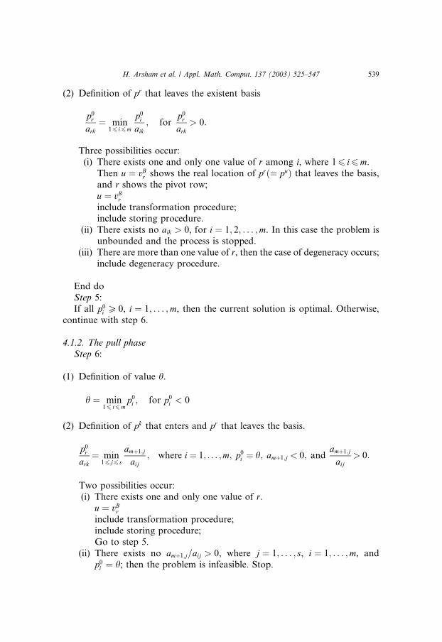
(2) Definition of pr that leaves the existent basis
Subscript r defines the pivot row (see, e.g., Ref. [4]) within A.Search for subscript r satisfying
p0rark
¼ min16 i6m
p0iaik
; forp0rark
> 0:
Four possibilities occur:
(i) vBr is already occupied then go to 1 to choose the next largest amþ1;j.(ii) There exists one and only one value of r among i, where 16 i6m.
Then u ¼ vBr shows the real location of prð¼ puÞ that leaves the basis,
and r shows the pivot row;u ¼ vBrinclude transformation procedure;
include storing procedure.
(iii) There exists no aik > 0, for i ¼ 1; 2; . . . ;m. In this case the problem isunbounded and the process is stopped.
(iv) There are more than one value of r, then the case of degeneracy occurs;Include degeneracy procedure.
End do
Step 4:Do while (there are amþ1;j > 0; j ¼ 1; . . . ; s)
(1) Define k of vector pk that enters the basis
pk ¼ max16 j6 s
amþ1;j; for amþ1;j > 0
Include step 3 (1.b.).
538 H. Arsham et al. / Appl. Math. Comput. 137 (2003) 525–547
(2) Definition of pr that leaves the existent basis
p0rark
¼ min16 i6m
p0iaik
; forp0rark
> 0:
Three possibilities occur:
(i) There exists one and only one value of r among i, where 16 i6m.Then u ¼ vBr shows the real location of p
rð¼ puÞ that leaves the basis,and r shows the pivot row;u ¼ vBrinclude transformation procedure;include storing procedure.
(ii) There exists no aik > 0, for i ¼ 1; 2; . . . ;m. In this case the problem isunbounded and the process is stopped.
(iii) There are more than one value of r, then the case of degeneracy occurs;include degeneracy procedure.
End do
Step 5:If all p0i P 0, i ¼ 1; . . . ;m, then the current solution is optimal. Otherwise,
continue with step 6.
4.1.2. The pull phase
Step 6:
(1) Definition of value h.
h ¼ min16 i6m
p0i ; for p0i < 0
(2) Definition of pk that enters and pr that leaves the basis.
p0rark
¼ min16 j6 s
amþ1;j
aij; where i¼ 1; . . . ;m; p0i ¼ h; amþ1;j < 0; and
amþ1;j
aij> 0:
Two possibilities occur:i(i) There exists one and only one value of r.
u ¼ vBrinclude transformation procedure;
include storing procedure;
Go to step 5.
(ii) There exists no amþ1;j=aij > 0, where j ¼ 1; . . . ; s, i ¼ 1; . . . ;m, andp0i ¼ h; then the problem is infeasible. Stop.
H. Arsham et al. / Appl. Math. Comput. 137 (2003) 525–547 539

4.2. Subroutine degeneracy
In case of degeneracy we iteratively, for j ¼ 1; 2; . . . ; d, divide the compo-nents of vector pj by the elements of A in the kth column. The process stopswhen pr have been found and defined.
e ¼ 1for g ¼ 1 to d(i) if (vg < 0) then
COMMENT. In this case pj is one of the basis vectors.j ¼ �vg(a) Build a vector p with its components pi ¼ 0, i ¼ 1; . . . ;m, i 6¼ j,and pj ¼ 1.(b) Search for subscript r satisfyingpr
ark¼ min16 i6m
pi
aik; for aik > 0:
(ii) else if (vg 6 s) thenCOMMENT. In this case pj is the jth column vector of A.j ¼ vgSearch for subscript r satisfying
pr
ark¼ min16 i6m
aij
aik; for aik > 0:
(iii) else if (vg 6 d) thenCOMMENT. In this case pj is one of the slack vectors.
(a) Define subscript j by the following procedurefor i ¼ e to m
if (qi ¼ 00P 00) thene ¼ iþ 1;j ¼ i;exit for
end if
end for
(b) Build a vector p with its components pi ¼ 0, i ¼ 1; . . . ;m, i 6¼ j,and pj ¼ �1.(c) Search for subscript r satisfyingpr
ark¼ min16 i6m
pi
aik; for aik > 0:
end if(iv) if there is one value for r then
COMMENT. In this case pr has been defined.
540 H. Arsham et al. / Appl. Math. Comput. 137 (2003) 525–547
u ¼ vBrexit for
end if
end for
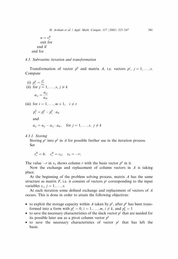
4.3. Subroutine iteration and transformation
Transformation of vector p0 and matrix A, i.e. vectors pj, j ¼ 1; . . . ; s.Compute
ii(i) p0r ¼p0rark
i(ii) for j ¼ 1; . . . ; s, j 6¼ k
arj ¼arj
ark
(iii) for i ¼ 1; . . . ;mþ 1, i 6¼ r
p0i ¼ p0i � p0r � aik
and
aij ¼ aij � arj � aik; for j ¼ 1; . . . ; s; j 6¼ k
4.3.1. Storing
Storing pr into pk in A for possible further use in the iteration process.Set
vBr ¼ h; cBr ¼ ch; vh ¼ �r;
The value �r in vh shows column r with the basis vector ph in it.Now the exchange and replacement of column vectors in A is taking
place.
At the beginning of the problem solving process, matrix A has the same
structure as matrix F, i.e. it consists of vectors pj corresponding to the input
variables xj, j ¼ 1; . . . ; s.At each iteration some defined exchange and replacement of vectors of A
occurs. This is done in order to attain the following objectives:
• to exploit the storage capacity within A taken by pk, after pk has been trans-
formed into a form with pki ¼ 0, i ¼ 1; . . . ;m, i 6¼ k, and pk
k ¼ 1• to save the necessary characteristics of the slack vector pr that are needed for
its possible later use as a pivot column vector pk
• to save the necessary characteristics of vector pr that has left the
basis.
H. Arsham et al. / Appl. Math. Comput. 137 (2003) 525–547 541

The process of replacement of pk by pr is as follows:
ii(i) if (qr ¼ 00P 00 and u ¼ 0) thenCOMMENT. In this case uth row in the basis is not occupied. A slackvector psþr is built up to the position of an auxiliary vector p, then trans-formed in accordance with the particular iteration and stored in the kthcolumn of A.(a) Build up psþr within an auxiliary vector p, where pi ¼ 0, i ¼
1; . . . ;mþ 1, i 6¼ r, and pr ¼ �1(b) Transform components of p accordingly:
pr ¼ prark
pi ¼ pi � pr � aik, i ¼ 1; . . . ;mþ 1, and i 6¼ r(c) Store p into the kth column of A:
aik ¼ pi, i ¼ 1; . . . ;mþ 1(d) Mark up the location of psþr by storing value k into the r þ sth com-
ponent of vector v:vrþs ¼ k
i(ii) else if (qr ¼ 00 ¼ 00 and u ¼ 0) thenCOMMENT. uth row in the basis is not occupied and there is no slackvector to be stored in the kth column of A.
(iii) elseCOMMENT. In this case u shows the real location (column) of pr
(¼ pu) that leaves the basis. pu is a basis vector with its com-
ponents pui ¼ 0, i ¼ 1; . . . ;m, i 6¼ r, and pu
r ¼ 1. In addition, pu can again
enter the basis in later stages of the iteration process. There-
fore it is transformed accordingly and saved in the location of pk
within A.(a) Build up pu within an auxiliary vector p, where pi ¼ 0, i ¼ 1; . . . ;m,
i 6¼ r, and pr ¼ 1(b) Transform components of p accordingly:
pr ¼ prark
pi ¼ pi � aik, i ¼ 1; . . . ;mþ 1, and i 6¼ r(c) Store p in the kth column of A: aik ¼ pi, i ¼ 1; . . . ;m(d) Mark up the location of pu by storing k in the uth component of vec-
tor v: vu ¼ kend if
5. Numerical illustrative example for the computer implementation
In this section we are applying the computer implementation technique tothe last numerical example solved earlier in Section 3.
542 H. Arsham et al. / Appl. Math. Comput. 137 (2003) 525–547

max 2X1 þ 3X2 � 6X3subject to X1 þ 3X2 þ 2X3 6 3
�2X2 þ X3 6 1
X1 � X2 þ X3 ¼ 22X1 þ 2X2 � 3X3 ¼ 0; where Xj P 0; j ¼ 1; . . . ; 3:
Step 1:
X1 þ 3X2 þ 2X3 þ X4 ¼ 3�2X2 þ X3 þ X5 ¼ 1
X1 � X2 þ X3 ¼ 22X1 þ 2X2 � 3X3 ¼ 0
Step 2:
ii(i) Read the input data:
mð¼ 4Þ, sð¼ 3Þ, c, p0ð¼ RHSÞ, Ai(ii) Read q, i.e., q ¼ ½006 00; 006 00; 00 ¼ 00; 00 ¼ 00�(iii) Compute
d ¼ 3(iv) Create
v ¼ ½1; 2; 3�
c ¼ ½2; 3;�6�
amþ1 ¼ ½2; 3;�6�
(v) Create
vB ¼ ½4; 5; 0; 0�
cB ¼ ½0; 0; 0; 0�
Step 3:
(1) Definition of vector pk that enters the basis
H. Arsham et al. / Appl. Math. Comput. 137 (2003) 525–547 543

(2) Definition of vector pr that leaves the basis
0=2; r ¼ 4; u ¼ vB4 ¼ 0
Transformation of p0 and pj, j ¼ 1; . . . ; s
Storing pr and pk
Set
vB4 ¼ 2cB4 ¼ 3v2 ¼ �4
Since q4 ¼ 00 ¼ 00 and u ¼ 0, the uth row in the basis is not occupied and there isno slack vector to be stored in the kth column of A.
5.1. Iteration 2
Step 3:
(1) Definition of vector pk that enters the basis
(2) Definition of vector pr that leaves the basis
2=2; r ¼ 3; u ¼ vB3 ¼ 0
544 H. Arsham et al. / Appl. Math. Comput. 137 (2003) 525–547

Transformation of p0 and pj, j ¼ 1; . . . ; s
Storing pr and pk
vB3 ¼ 1cB3 ¼ 2v1 ¼ �3
Since q3 ¼ 00 ¼ 00 and u ¼ 0, the uth row in the basis is not occupied and there isno slack vector to be stored in the kth column of A.
5.2. Iteration 3
Step 3:
The basis is completed. Therefore continue with step 4.
Step 4:
All amþ1;j 6 0, j ¼ 1; . . . ; s. Continue with step 5.Step 5:
Some of p0i 6 0, i ¼ 1; . . . ;m. Continue with step 6.Step 6: Pull phase
(1) Definition of h.
h ¼ �1; p02 ¼ �1; p04 ¼ �1(2) Definition of vectors pk and pr.
amþ1;3 ¼ �7=4; k ¼ 3; h ¼ 3amþ1;3
a2;3¼ 76;
amþ1;3
a4;3¼ 75; r ¼ 2; u ¼ vB2 ¼ 5
H. Arsham et al. / Appl. Math. Comput. 137 (2003) 525–547 545
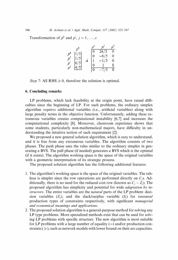
Transformation of p0 and pj, j ¼ 1; . . . ; s
Step 7: All RHSP 0, therefore the solution is optimal.
6. Concluding remarks
LP problems, which lack feasibility at the origin point, have raised diffi-
culties since the beginning of LP. For such problems, the ordinary simplex
algorithm requires additional variables (i.e., artificial variables) along withlarge penalty terms in the objective function. Unfortunately, adding these ex-
traneous variables creates computational instability [6,7] and increases the
computational complexity [8]. Moreover, classroom experience shows that
some students, particularly non-mathematical majors, have difficulty in un-
derstanding the intuitive notion of such requirement [2].We proposed a new general solution algorithm, which is easy to understand,
and it is free from any extraneous variables. The algorithm consists of two
phases. The push phase uses the rules similar to the ordinary simplex in gen-
erating a BVS. The pull phase (if needed) generates a BVS which is the optimal
(if it exists). The algorithm working space is the space of the original variables
with a geometric interpretation of its strategic process.
The proposed solution algorithm has the following additional features:
1. The algorithm�s working space is the space of the original variables. The tab-leau is simpler since the row operations are performed directly on Cjs. Ad-
ditionally, there is no need for the reduced cost row (known as Cj � Zj). The
proposed algorithm has simplicity and potential for wide adaptation by in-structors. The entire variables are the natural parts of the LP problem: deci-sion variables (Xj), and the slack/surplus variable (Si) for resource/
production types of constraints respectively, with significant managerialand economical meanings and applications.
2. The proposed solution algorithm is a general-purpose method for solving any
LP type problems. More specialized methods exist that can be used for solv-
ing LP problems with specific structure. The new algorithm is most suitable
for LP problems with a large number of equality (¼) and/or production con-straints (P), such as networkmodels with lower bound on their arc capacities.
546 H. Arsham et al. / Appl. Math. Comput. 137 (2003) 525–547

3. It is well known that the initial basic solution by the primal simplex could be
far away from the optimal solution [10]. The BVS augmentation conceptwhich pushes toward faces of the feasible region which may contain an op-timal rather than jumping from a vertex to an improved adjacent one to pro-
vide a ‘‘warm-start’’.
4. Its computer implementation leads to further reduction of simplex tableau.
This means a smaller amount of computer storage is needed to store the tab-
leau and also a faster iteration. This fact could be very important particu-
larly in solving large problems of linear programming.
Areas for future research are looking for any possible refinement, and the
development of efficient code to implement this approach, and then perform a
comparative study. At this stage, a convincing evaluation for the reader would
be the application of this approach to a problem he/she solved by any other
methods.
Acknowledgements
We are deeply grateful to the referees for their careful readings and useful
suggestions. The National Science Foundation Grant CCR–9505732 supported
this work.
References
[1] H. Arsham, Affine geometric method for linear programs, Journal of Scientific Computing 12
(3) (1997) 289–303.
[2] H. Arsham, Initialization of the simplex algorithm: an artifical-free approach, SIAM Review
39 (4) (1997) 736–744.
[3] H. Arsham, Distribution-routes stability analysis of the transportation problem, Optimization
43 (1) (1998) 47–72.
[4] V. Chvatal, Linear Programming, Freeman and Co., New York, 1993.
[5] G. Dantzig, Linear Programming and Extensions, Princeton University Press, NJ, 1968.
[6] T. Gao, T. Li, J. Verschelde, M. Wu, Balancing the lifting values to improve the numerical
stability of polyhedral homotopy continuation methods, Applied Mathematics and Compu-
tation 114 (2–3) (2000) 233–247.
[7] V. Lakshmikantham, S. Sen, M. Jain, A. Ramful, Oðn3Þ Noniterative heuristic algorithm forlinear programs with error-free implementation, Applied Mathematics and Computation 110
(1) (2000) 53–81.
[8] G. Mohr, Finite Element modelling of distribution problems, Applied Mathematics and
Computation 105 (1) (1999) 69–76.
[9] K. Papparrizos, The two-phase simplex without artificial variables, Methods of Operations
Research 61 (1) (1990) 73–83.
[10] A. Ravindran, A comparison of the primal-simplex and complementary pivot methods for
linear programming, Naval Research Logistic Quarterly 20 (1) (1973) 95–100.
[11] H. Taha, Operations Research: An Introduction, Macmillan, New York, 1992.
H. Arsham et al. / Appl. Math. Comput. 137 (2003) 525–547 547