An E�cient Steepest-Edge SimplexAlgorithm for SIMD ComputersMichael E. Thomadakis and Jyh-Charn LiuDepartment of Computer ScienceTexas A&M UniversityCollege Station, TX 77843{3112fmiket,jcliug@cs.tamu.eduTR96-032January 30, 1996AbstractThis paper proposes a new parallelization of the Primal and Dual Simplex algorithms forLinear Programming (LP) problems on massively parallel Single-Instruction Multiple-Data(SIMD) computers. The algorithms are based on the Steepest-Edge pivot selection method andthe tableau representation of the constraint matrix. The initial canonical tableau is formed onan attached scalar host unit, and then partitioned into a rectangular grid of sub-matrices anddistributed to the individual Processor Element (PE) memories. In the beginning of the parallelalgorithm key portions of the simplex tableau are partially replicated and stored along with thesub-matrices on each one of the PEs. The SIMD simplex algorithm iteratively selects a pivotelement and carries-out a simplex computation step until the optimal solution is found, or whenunboundedness of the LP is established. The Steepest-Edge pivot selection technique utilizesinformation mainly from local replicas to search for the next pivot element. The pivot row andcolumn are selectively broadcasted to the PEs before a pivot computation step, by e�cientlyutilizing the geometry of the toroidal mesh interconnection network. Every individual PEmaintains locally and keeps consistent its replicas so that inter-processor communication due todata dependencies is further reduced. The presence of a pipelined inteconnection network, likethe mesh network of MP-1 and MP-2 MasPar models allows the global reduction operationsnecessary in the selection of pivot columns and rows to be performed in time O(log nR +log nC), in (nR � nC) PE arrays. This particular combination of pivot selection, matrixrepresentation, and selective data replication is shown to be highly e�cient in the solution oflinear programming problems on SIMD computers. The proposed parallelization has optimalasymptotic speedup and scalability properties. Performance comparisons show that as the1

2problem sizes increase the speed-ups obtained by MasPar's MP-1 and MP-2 models are in theorder of 100 times, and 1000 times, respectively, over sequential versions of the Steepest-EdgeSimplex algorithm running on high-end Unix workstations.Index Terms: Single-Instruction Multiple-Data (SIMD), Simplex Algorithm, Steepest-EdgePivot Selection, Matrix Partitioning, Dense Representation, Data Replication, Global Reduc-tions, Pipelined Networks.

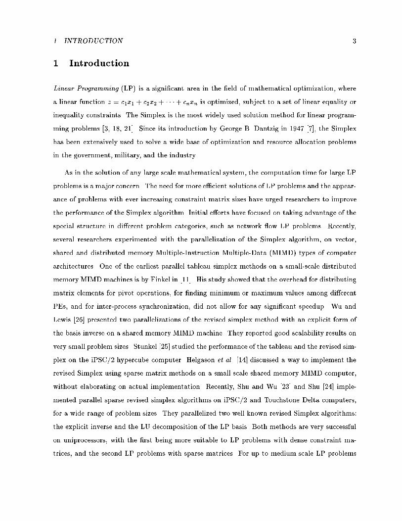
1 INTRODUCTION 31 IntroductionLinear Programming (LP) is a signi�cant area in the �eld of mathematical optimization, wherea linear function z = c1x1 + c2x2 + � � �+ cnxn is optimized, subject to a set of linear equality orinequality constraints. The Simplex is the most widely used solution method for linear program-ming problems [3, 18, 21]. Since its introduction by George B. Dantzig in 1947 [7], the Simplexhas been extensively used to solve a wide base of optimization and resource allocation problemsin the government, military, and the industry.As in the solution of any large scale mathematical system, the computation time for large LPproblems is a major concern. The need for more e�cient solutions of LP problems and the appear-ance of problems with ever increasing constraint matrix sizes have urged researchers to improvethe performance of the Simplex algorithm. Initial e�orts have focused on taking advantage of thespecial structure in di�erent problem categories, such as network ow LP problems. Recently,several researchers experimented with the parallelization of the Simplex algorithm, on vector,shared and distributed memory Multiple-Instruction Multiple-Data (MIMD) types of computerarchitectures. One of the earliest parallel tableau simplex methods on a small-scale distributedmemory MIMD machines is by Finkel in [11]. His study showed that the overhead for distributingmatrix elements for pivot operations, for �nding minimum or maximum values among di�erentPEs, and for inter-process synchronization, did not allow for any signi�cant speedup. Wu andLewis [26] presented two parallelizations of the revised simplex method with an explicit form ofthe basis inverse on a shared memory MIMD machine. They reported good scalability results onvery small problem sizes. Stunkel [25] studied the performance of the tableau and the revised sim-plex on the iPSC/2 hypercube computer. Helgason et al. [14] discussed a way to implement therevised Simplex using sparse matrix methods on a small scale shared memory MIMD computer,without elaborating on actual implementation. Recently, Shu and Wu [23] and Shu [24] imple-mented parallel sparse revised simplex algorithms on iPSC/2 and Touchstone Delta computers,for a wide range of problem sizes. They parallelized two well known revised Simplex algorithms:the explicit inverse and the LU decomposition of the LP basis. Both methods are very successfulon uniprocessors, with the �rst being more suitable to LP problems with dense constraint ma-trices, and the second LP problems with sparse matrices. For up to medium scale LP problems

1 INTRODUCTION 4the explicit form of inverse method attained reasonable speedup. The LU decomposition simplexon the Toughstone Delta was able to show some speedup only on large and sparse problems.Their sparse simplex parallelization experienced high communication to computation ratio on theTouchstone machine due to strong data dependencies between PEs. Simplex algorithms for gen-eral linear programming problems on (Single Instruction Multiple Data stream) SIMD computershave been reported by Agarwal et al. in [1], and by Eckstein et al. in [10]. The early implemen-tation in [1] had a disappointing performance. Eckstein et al. in [10] implemented prototypes ofdense simplex and interior-point algorithms on a CM-2 machine. They concluded that interiorpoint algorithms are relatively easy to implement on SIMD machines with commercially availablelibrary software. On the other hand, an e�cient parallel implementation of the simplex methodwould require careful attention to data placement and low-level data motion, which is di�cult toexpress in current data-parallel high-level languages.The main focus of this paper is on the design of scalable Primal and Dual Simplex methods forSIMD multiprocessor systems. We present an e�cient massively parallel solution to general LPproblems with dense constraint matrices. Dense LP sub-problem are typically found in Bender'sor Dantzig-Wolfe decompositions of large LP problems, or as sub-problems in integer LP problems.Our algorithm is based on the Two-Phase tableau method and the Steepest-Edge pivot selectiontechnique. It forms and distributes the canonical simplex tableau X onto the memories of thePE grid. Simplex continuously examines and modi�es the reduced cost row and the current basicfeasible solution column of the tableau. The parallel algorithm mitigates data dependencies ineach iteration between distant PEs by partially replicating these particular tableau parts to allPEs. By maintaining local replicas our algorithm eliminates the need for continuously distributingthese tableau portions to the rest of the PEs, thus reducing inter-PE communication overhead.The local data replicas maintain su�cient information for the PEs to perform pivot computationsteps, and make decisions about the next pivot step in parallel. Pivot rows and columns areselectively distributed to the PEs before every pivot step. Since each PE stores a rectangular sub-block of the tableau, it needs to receive the portions of the pivot row and column correspondingto this sub-block only, and not the entire pivot row and column. The individual data movementstake place only along the horizontal and the vertical directions of the PE array, and they proceed

2 THE SEQUENTIAL STEEPEST-EDGE SIMPLEX ALGORITHM 5in parallel. In each PE row or column one PE is the source and the rest of the PEs in the same rowor column are the recipients. This origin-destination inter-PE communications pattern utilizese�ciently toroidal mesh interconnection networks commonly available in modern SIMD machines.The algorithm achieves high e�ective communication bandwidth, especially in machines where apipelined network is available.We assess the performance of the proposed method by solving LP problems with di�erenttableaux sizes on MasPar's MP-1 and MP-2 models. A sequential version of the steepest-edgesimplex has solved the same test problems on a Unix SPARC server 1000 workstation. The solutione�ort in terms of average computation (SPARC 1000, MP-1 and MP-2) and communication(MP-1 and MP-2) time per simplex iteration is measured so that comparisons can be madebetween sequential and massively parallel methods. Our performance experiments show that theparallel version running on a 16,384 PE MP-2 achieves execution speedups of the order of 1,000to 1,200 times over the sequential version of the algorithm. These speedup results demonstratethe e�ectiveness of a parallel steepest-edge tableau method on SIMD multiprocessors.The rest of this paper is organized as follows. Section 2 brie y overviews the scalar PrimalSimplex method it analyzes its asymptotic time and presents timing results from our computa-tional experiments with the scalar simplex code. Section 3 develops the SIMD Steepest-EdgeSimplex algorithm, it analyzes its performance and scalability, and presents execution time mea-surements on the MP-1 and MP-2 MasPar models. Finally, section 4 discusses the factors whichallow the steepest-edge simplex to attain high speedup results.2 The Sequential Steepest-Edge Simplex AlgorithmLinear Programming (LP) problems are usually formulated in the general form, where a linearfunction z = c1x1+ c2x2+ � � �+ ckxk, in k variables, is minimized or maximized, while it satis�esa set of linear equality or inequality constraints, and xj � 0, or xj><0, for j = 1; 2; : : : ; k. EveryLP problem in the general form can be expressed into an equivalent LP [9, 21] in the standardform. In this paper without loss of generality we consider minimization types of LP problems, in

2 THE SEQUENTIAL STEEPEST-EDGE SIMPLEX ALGORITHM 6the standard form, de�ned asMinimize z = c1x1+ c2x2 + � � �+ cnxnSubject to a11x1+ a12x2 + � � �+ a1nxn = b1a21x1+ a22x2 + � � �+ a2nxn = b2... . . . ...am1x1+am2x2 + � � �+ amnxn = bmand xj � 0; j = 1; 2; : : : ; n: (1)or more compactly expressed in vector notationminz = c0x (2)Ax = bx � 0;where, A is a m � n constraint coe�cient matrix, c0 2 Rn the cost coe�cients row vector, andb 2 Rm the right-hand side (RHS) column vector of constants. Any x 2 Rn such that Ax = bis called a feasible point, and the convex polytope F = fx 2 Rn : Ax = b;x � 0g forms thefeasible space of the given LP problem, for which we assume F 6= ;. Any collection of m linearlyindependent columns of matrix A, denoted by B = fAB(i) : i = 1; 2; : : : ; mg, is called a basisof A, and in the present discussion B(i) = j means that the ith vector of this basis is the jthcolumn of A. Any given basis B partitions matrixA into two submatrices N and B, denoted byA = [N jB]. N is a m� (n�m) submatrix ofA formed by (n�m) non-basic columns. Similarly,B is a m�m submatrix which consists of the m basic columns of A. Given a basis B , a vectorx 2 Rn which expresses RHS b of (2) as a linear combination of the m columns B of A, is calleda basic feasible solution (BFS) of the LP. In any BFS the (n �m) components associated withthe non-basic columns are equal to zero and the rest m components1, associated with the basiccolumns, are positive numbers. If we denote a BFS by x = [xN jxB]T = [0jxB ]T , then we haveAx = NxN +BxB = BxB = b;and, xB = B�1b. The cost value z of the objective function at a BFS x is given byz = c0BxB = c0B�1b:It is well known [9, 21] that every BFS x 2 F is a vertex (i.e., a corner point) of convex polytope F ,and that the optimal solution, denoted by x�, is also a vertex of F . The simplex algorithm starts1Ignoring the problem of degeneracy.

2 THE SEQUENTIAL STEEPEST-EDGE SIMPLEX ALGORITHM 7from some initial BFS x(0) and by applying successive transformations on the constraint matrixA, called simplex pivot steps, it generates a sequence x(1);x(2); : : : ;x(k) of BFSs'. For the values ofthe cost function z0; z1; : : : ; zk evaluated at the BFSs we have that zi � zi�1, so that after a �nitenumber k of pivot steps the optimal BFS x� = x(k) is found, where z� = c0x� = minfc0x : x 2 Fg.When simplex moves from BFS x(i�1) to BFS x(i), a new basis B(i) is formed, by allowing a non-basic component of x(i�1) to become positive, while letting a basic one to drop to zero, andadjusting the rest in a way that maintains primal feasibility. A pivot operation obtains thenew basis B(i), by removing a \less" pro�table column, Al 2 B(i�1), and introducing a \more"pro�table non-basic column Aj 62 B(i�1) of A, into the current basis. A column Aj 62 B ofA is considered to be pro�table only if its reduced cost coe�cient �cj is less than zero, where�cj = cj�c0BB�1Aj = cj�c0BXj . �cj is the amount by which the cost function value changes whencomponent xj of x increases by one unit, while the basic components are adjusted by quantity�Xj , where Xj = B�1Aj . Simplex reaches the optimal BFS x� when �cj � 0; j = 1; 2; : : : ; n,that is, when there no other pro�table columns to introduce into the current basis.The tableau simplex method maintains a representation Xj of the columns Aj of constraintmatrixA, and the RHS vector b in terms of the basis B associated with a given BFS x. If B is thebasic submatrix of A associated with x, we set X0 = B�1b, and Xj = B�1Aj ; j = 1; 2; : : : ; n.Simplex maintains in a compact form in the tableau matrix X columns Xj ; j = 0; 1; : : : ; n, androw vector �c0. X is a (m+ 1)� (n+ 1) matrix where row 0 is equal to the reduced cost row �c0,and the remaining lower m rows form a m� (n+ 1) submatrix which consists of column vectorsX0; X1; : : : ; Xn, as follows:X = �z �c0B�1[bjA] = �z �c1 �c2 : : : : : : �cnX0 X1 X2 � � � � � � Xn ; (3)where, �z = 0� c0BB�1b = �c0BxB of BFS x.At each pivot step simplex uses a pivot selection heuristic to choose one pro�table column tointroduce into the basis, among those with negative reduced cost coe�cient. Once a new pivotcolumn Xj of X is selected, simplex determines the pivot row x0i, where i is the row that satis�es

2 THE SEQUENTIAL STEEPEST-EDGE SIMPLEX ALGORITHM 80 1 2 3 4 1N− N5

01

M

2

1M−

j

i

Candidate pivot columns

0 1 2 3 4 1N− N5

01

M

2

1M−

j

i

Coefficients in pivot row ix

Tableau coefficients

i,jxCurrent pivot element

jXpivot column

currentpivotrow

The next pivot element isi,jx

xkl

x i

a b

Candidate pivot column Xl

Modified cost row < 0cl

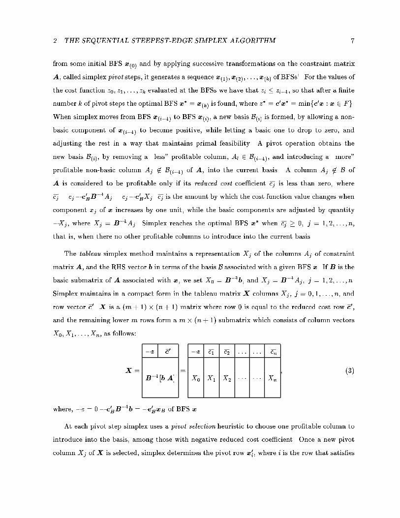
Coefficients in pivot column XjFigure 1: a. The candidate columns Xj with �cj < 0 are scattered throughout tableau X. b. Thepivot row x0i, column Xj , and, element xij on the Simplex tableau X for the scalar algorithmthe minimum-ratio condition�i = xi0xij = min(xk0xkj ; k = 1; 2; : : : ; m; xkj > 0) : (4)Then simplex performs a pivot operation on xij and it generates a new tableau �X from X . �Xre ects a representation with respect to the resulting new basis �B. The elements of the newtableau are computed as follows:�xkl = 8><>: xkl � xkj xilxij ; k = 0; 1; : : : ; m; k 6= i;xklxij ; k = i; (5)for l = 0; 1; : : : ; n. Figure (1.a) shows a typical tableau X con�guration before a pivot step.Columns Xl with reduced cost coe�cient �cl < 0 are scattered throughout the tableau. In Fig-ure (1.b), Xj is the next pivot column, x0i as the pivot row, and xij is the next pivot element.The reduced cost row �c0 is shown as the top shaded row, and the BFS column X0 is the shaded,leftmost column in Figures (1.a, b). From Eq. (5) it is clear that element �xkl of the resultingtableau depends on elements xij ; xil; xkj , and xkl of the previous tableau. One of the most widelyused pivot selection methods is the Dantzig's rule[9], where simplex always selects as pivot columnXj the one with the most negative reduced cost coe�cient �cj = minf�ck < 0 : k = 1; 2 : : : ; ng.This method has been employed in all previous simplex method parallelizations. Other pivot se-

2 THE SEQUENTIAL STEEPEST-EDGE SIMPLEX ALGORITHM 9lection heuristics include the Bland's [21], the Least-Recently Considered [19], the maximum costreduction [21, 22], Partially Normalized [5], the \DEVEX" [13], and the Steepest-Edge [12, 22]rules. Drawing on our previous computational experience with these pivot selection methodswe decided to use the Steepest-Edge method, since i) this method constantly guides simplex totake the fewest pivot steps to �nd the optimal solution compared to the other methods, and ii)the searching for the pivot column and row are scalable and this makes it a natural choice fora massively parallel version of a simplex algorithm, like the one we present in section 3. Thesteepest-edge method selects the column Xj with the most negative quantity �j , where�j = �cjkdjk = min8<: �ckq1 +Pmi=1 x2ik ; k = 1; : : : ; n; �ck < 09=; : (6)Our sequential simplex caries out a pivot computation on the (n � m) non-basic tableaucolumns, one at a time and at the same time it accumulates sums of squares SSQk = 1+Pmi=1 x2ikof the coe�cients for each column Xk with �ck < 0. Then it searches all candidate columnssequentially for the minimum quantity �j .Our scalar and parallel simplex methods rely on the two phase technique to obtain an initialBFS. Both share a basic common portion of code to load an LP problem into memory and preparethe initial \canonical" tableau matrixX . Then simplex is invoked to �nd the solution and collecttiming measurements. The common code is summarized as follows:1. De�ne Tableau X, and other variables;2. Retrieve input LP problem data into memory;3. Add slack/surplus and arti�cial variables, as necessary, to form Simplex tableau X and gothrough Phase I;4. Check after Phase I if LP is infeasible, and if it is STOP;5. Otherwise, remove arti�cial variables and redundant rows, and proceed to simplex PhaseII, starting from the basis B obtained from Phase I;6. Save results and measurements to report �les, and EXIT;

2 THE SEQUENTIAL STEEPEST-EDGE SIMPLEX ALGORITHM 10Algorithmic Steps Asymptotic ComplexityProc Sequential Simplex(X)let OPT = FALSE; /* Not optimal yet */let UNB = FALSE; /* Not unbounded feasible space F */Compute the reduced cost row coe�cients �c0 �(m� n)Find the �rst pivot element xij ; Xj has minf�cj : j = 1; : : : ; ng; O(n)while (not OPT and not UNB) do nPPerform pivot computation described in Eq. (5);Divide pivot row x0i by xij;let xil = xilxij ; l = 0; 1; : : : ; n; �(n)Update reduced cost row: �c0;let �cl = �cl � �c0jxil; k = 0; 1; : : : ; n; �(n)Update remaining tableau coe�cients;for k = 1; 2; : : : ; m; k 6= i; l = 1; 2; : : : ; n; l 6= j; Aj 62 B do �(m� (n�m))let xkl = xkl � xilxkj ;if (�cl < 0) then let SSQ = SSQ+ x2kl; endifendforif (�cl � 0; l = 1; 2; : : : ; n) thenlet OPT = TRUE; /* We are at optimal bfs x� */elseUse Steepest-Edge pivot selection technique to locatethe next incoming column Xj of Tableau X ;Select Xj with �j = min( �clp1 + SSQl : �cl < 0; l = 1; 2; : : : ; n); O(n�m)if (xkj � 0; k = 1; 2; : : : ; m) thenlet UNB = TRUE; /*F is unbounded */elseFind �i = xi0xij = minfor allxkj>0(xk0xkj : k = 1; 2; : : : ; m) ; �(m)endifendifendwhileEndproc Figure 2: The sequential Steepest-Edge simplex algorithm

2 THE SEQUENTIAL STEEPEST-EDGE SIMPLEX ALGORITHM 11The core of the sequential Steepest-Edge algorithm is presented in Fig. (2). The tableau Xhas m+ 1 rows and n + 1 columns, as explained previously. The while : : :do loop iterates oncefor each simplex pivot step, until the optimal BFS x� is found or the LP problem is determinedto be unbounded (min z = �1). The number of times nP that the loop iterates is LP problem(and pivot selection method) dependent. We are interested in the computational complexity ofeach pivot step, so we consider only the statements inside the while loop. The algorithm �rstdivides the current pivot row x0i by the pivot element xij , and updates the reduced cost row, eachin �(n) steps. It carries out the pivot operation on all the non-basic columns of the tableau in�(m� (n�m)) steps. At the same time if the column under update Xj has �cj < 0 it accumulatespartial sums SSQj , needed for the searching of the next pivot element by the steepest-edge (6),in in O(m� (n�m)) steps. Finally, it locates the next entering column Xj and pivot element xijin �(n), and �(m) steps, respectively. To summarize we have the followingComplexity of pivot computationT scomp(m;n) = �(m� (n�m)) + 2�(n) = �(m� (n�m)) (7)Complexity of Steepest-Edge pivot searchT sse(m;n) = O(m� (n�m)) +O(n�m) + �(m) = O(m� (n�m)) (8)Total complexity of sequential Steepest-Edge simplexT stotal(m;n) = �(m� (n�m)) (9)Given that simplex needs nP pivots to solve a problem, the total computation complexity untiloptimal solution is �(nP �m� (n�m)).Most performance measurements reported in the literature show the total time until the so-lution of some LP problem of a certain size. For the same LP problem di�erent pivot selectionmethods generate a di�erent number of pivot steps. On the other hand the average time ina pivot step is a more accurate metric of the resource requirements for a pivot selection andcomputation methods of a speci�c simplex implementation. It may also be used to make direct

3 SIMD STEEPEST-EDGE SIMPLEX ALGORITHM 120

20

40

60

80

100

120

140

0 10000 20000 30000 40000 50000 60000

Tim

e in

Sec

onds

Number of Columns

SPARC 1000: Average Time / Scalar Simplex iteration

4,0963,0722,0481,024

51225664

Figure 3: The Average execution times per scalar Steepest-Edge Simplex iteration versus numberof columns in tableau X, with 64, 256, 512, 1024, 2048, 3072, and 4096 rowsperformance comparisons between sequential and parallel implementations. For this reason wereport and make our performance comparisons based on the average time taken for each pivotstep. The steepest-edge simplex algorithm is implemented in the C language. All the experimentswere conducted on a Sun SPARC Server 1000 Unix workstation, with 64MB of main memory.In the code all variables are 8 byte double precision reals. For each LP problem with a certainnumber of rows we perform many numerical experiments, increasing the number of columns untilmemory capacity is reached. Figure 3 plots the execution times of LP problems with 64, 256, 512,1024, 2048, 3072, and 4096 rows. When the number of rows is relatively small, e.g., 64 or 256,the average time for each iteration increases slowly as we increase the number of columns. Asthe number of rows in the LP tableau becomes more than 1000 rows, the average time for eachiteration increases sharply with the number of columns.3 SIMD Steepest-Edge Simplex AlgorithmThe discussion of this section assumes that the target SIMD computer is a PE array with nR rowsand nC columns of PEs interconnected in a torus mesh topology, and that the tableauX of the LP

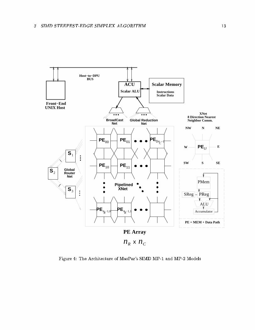
3 SIMD STEEPEST-EDGE SIMPLEX ALGORITHM 13 Front−End UNIX Host

Scalar MemoryACUScalar ALU

BroadCast Net

Global Reduction Net

PE Array

nR nCx

PE00 PE01PE n0 −1C

PE11PE10

PEnR−1,0 PEnR−1,1

Pipelined XNet

PMem

PReg

ALU

Accumulator

SReg

PE = MEM + Data Path

PEIJ

N

S

EW

NW NE

SW SE

XNet8 Direction Nearest Neighbor Comm.

Host−to−DPU BUS

InstructionsScalar Data

S1

S3

GlobalRouter Net

S2

Figure 4: The Architecture of MasPar's SIMD MP-1 and MP-2 Models

3 SIMD STEEPEST-EDGE SIMPLEX ALGORITHM 14is a (m+1)�(n+1) matrix. We use the notation PE[I;J], I = 0; 1; : : : ; nR�1; J = 0; 2; : : : ; nC�1,to refer to PE with coordinates (I; J). From the analysis in section 2, we observe that in eachiteration step the algorithm performs mainly two activities: i) simplex pivot computation, whichtakes time �(m�(n�m)), and ii) pivot column and row search, which takes timeO(m�(n�m)).We note that the data dependencies in the pivot computation of any tableau element xkl in i), asdetermined by Eq. (5), are with elements xkj of the pivot column Xj , xil of pivot row x0i, and xklitself. This was depicted in Fig. (1.b) of section 2 by the two arrows emanating from a tableauelement and reaching the corresponding pivot column and row positions. For ii) simplex needs toutilize information from: a) the reduced cost coe�cients row �c0, and b) the current BFS columnX0. We may partition the tableau X into a rectangular arrangement of nR � nC submatricesXIJ ; I = 0; 1; : : : ; nR� 1; J = 0; 1; : : : ; nC � 1 and distribute them to the nR � nC di�erent PEsof the SIMD machine. We expect that data dependencies to data in remote PEs for i) and ii)will generate high communication requirements. Additionally, PEs which need to receive commondata values broadcasted from some PE would have to wait until this PE transmits it to them, onePE at a time, and this will further decrease the degree of concurrent processing. To avoid thesepotential communication bottlenecks our approach is i) to selectively broadcast the current pivotcolumn and row to the PEs before each pivot step, and ii) replicate the reduced cost row and thecurrent BFS column of the tableau X to all PEs in the beginning of the algorithm and then leteach PE maintain them locally. The broadcast in i) allows the PEs to receive the data they needall at once without having to request and receive it in sequential order from the sending PEs. Thereplication in ii) makes information stored in remote PEs already present when a PE needs it todetermine the next pivot element, thus saving repetitive communication.In our parallel simplex algorithm, after an LP problem is retrieved for solution, the canonicaltableauX is formed on the scalar host of the MasPar SIMD machine in exactly the same way as inour sequential algorithm. In the next step the program partitionsX into nR�nC sub-blocks XIJand distributes them to the individual PEmemories, so that, PE[IJ] receives submatrixXIJ . Eachsub-matrix has nr�1 = mnR rows and nc�1 = nnC columns, andXIJ is assigned tableau coe�cientsxij with i 2 fI � (nr� 1)+1; : : : ; (I+1) � (nr � 1)g and j 2 fJ � (nc� 1)+1; : : : ; (J +1) � (nc� 1)g.At this stage the arrangement of the sub-matrices in the PEs looks much like part a. of Fig. 5.

3 SIMD STEEPEST-EDGE SIMPLEX ALGORITHM 15PE

00PE

01PE

02PE

03

PE10

PE11

PE12

PE13

XScalar tableau

Prepared on scalarfront−end host.

Stored on the PE grid of theSIMD machine.

Replicated cost sub−rows

Replicated bfs sub−columns

Replicated pivot sub−rows

Replicated pivot sub−columns

Tableau coefficients i,jx

a.

b.

n

n

nr

012

n−1r

m

0 1 2 ncnc−1

c.xkl

11X X12X10 X13

X01 X02X00 X03

nc0 1 2 nc−1

nr

012

n−1r

m

0

1

2

n−1r

0 1 2 nc−1

SSQ PEIJ

on

X IJ on PEIJFigure 5: The data lay-out of the original tableau X stored on the local memories of a 2� 4 gridof PEs

3 SIMD STEEPEST-EDGE SIMPLEX ALGORITHM 16The reduced cost row is only stored in the memories of the top row of the PE grid, so that,the �rst nc � 1 coe�cients are stored on PE[0;0], the second nc � 1 on PE[0;1], and so on, andthe current BFS is stored in the leftmost column in the PEs in PE column 0, where the �rstnr � 1 coe�cients are on PE[0;0], the next nr � 1 on PE[1;0], and so on. Before the SIMD simplexiterative steps the algorithm augments every PE sub-matrix XIJ with two additional rows andtwo columns, to store the replicated tableau portions, and a vector SSQ as shown in Fig. 5c.The two rows have indices 0 and nr and the columns indices 0 and nc. Then the reduced costrow �c0 and the current BFS X0 are partially replicated to all PEs in the following fashion. EachPE[I;J], I = 1; : : : ; nR � 1; J = 1; : : : ; nC � 1 receives a copy of �c0 into its zeroth row fromPE[0;J] and a copy of X0 from PE[I;0] into its zeroth column. This is shown in Fig. 5b wherein each XIJ the shaded top row is a replica of the corresponding portion of the reduced costrow �c0 and the shaded leftmost column a replica of the corresponding portion of the current BFScolumn X0. After the initial replication all PEs in the same PE column have identical top rows,and all PEs in the same PE row have identical leftmost columns. In the parallel algorithm apivot column and row are chosen before each pivot step according to the steepest-edge methodand are selectively broadcasted to the PEs. The shaded rightmost column nc and the bottomrow nr of each submatrix XIJ , shown in Fig. 5c, are reserved to receive a copy of a portion ofthe currently chosen pivot column and the pivot row, respectively, In the same �gure we maysee the data dependencies before a pivot step for the computation of elements �xkl of the nexttableau, by Eq. (5) are restricted to data which is stored locally in each PE, and thus, we havee�ectively eliminated the need for any further communication steps. In the example of Fig. (5) a(m+ 1)� (n+ 1) tableau X is partitioned into a (nR�nC) grid of submatrices. Each submatrixhas (nr � 1)� (nc � 1) elements. In this example nr = 8=2 + 1 = 5; nc = 36=4 + 1 = 10; nR = 2,and nC = 4. On each PE the parallel algorithm maintains a \miniature" or complete sub-tableauof the initial canonical simplex tableau X.After the PE submatrices have been prepared the parallel algorithm enters the pivot iterationphase. For the next pivot column and row selection, simplex needs to consult the reduced costcoe�cients �c0, the current basic elements in columnX0. In the parallel simplex all PEs participatein the search for candidate pivot column and row simultaneously, since all this information is

3 SIMD STEEPEST-EDGE SIMPLEX ALGORITHM 17maintained in the local replicas. All PEs keep the replicated reduced cost coe�cient row andcurrent BFS column consistent throughout the execution of the algorithm by updating them withthe pivot operation as if they were another regular row and column of the tableau. Without thelocal replicas each PE would have to request the current reduced cost row from the PEs on the topPE row, and the current BFS from the PEs in the leftmost PE column. In all PEs the algorithmperforms the pivot computation in parallel and computes the partial sums SSQj = Pnri=1 x2ij foreach columnXj inXIJ with �cj < 0. After all sub-matrices have been updated the algorithm addsthe partial sums in the PEs in the same PE column together using a binary tree addition methodto form total sums for each column which are collected in the bottom row PEs. The bottom rowPEs then cooperate among themselves to locate the tableau column XPEj with global minimum�l = �cl=p1 + SSQl; l = 1; : : : ; n and the PE column PEJ storing this column. The PEs in the PEcolumn, say PEJ , work then in parallel to locate the next pivot row. They compute the \global"minimum ratio condition in two steps. In the �rst step each PE[I;PEJ] for I = 0; 1; : : : ; nR � 1locates the row with the minimum ratio condition among the rows of submatrix XI;PEJ . Thisutilizes information from the local replicas of the current BFS column stored on these PEs. Inthe second step the the same PEs cooperate to locate the row with the \global" minimum ratiocondition, using again a binary tree minimum �nding algorithm.After the next pivot column and row have been located the algorithm will broadcast themselectively to all PEs. To avoid complex notation we will refer to the next pivot column as Xjand the next pivot row as x0i. We note that the di�erent parts of pivot column Xj are stored inthe PEs in PE column PEJ . Similarly, the di�erent parts of pivot row x0i are stored in the PEsin PE row PEI . We selectively broadcast the elements of the pivot column row-wise as shown inFig. (6.a). All PEs in the same PE row I = 0; 1; : : : ; nR � 1, receive the same chunk of the pivotcolumn. Similarly, all PEs in a PE column J = 0; 1; : : : ; nC � 1, receive the same chunk of pivotrow elements as shown in Fig. (6b). This type of communication utilizes naturally the geometryof the toroidal mesh interconnection network of SIMD computers of the MasPar's MP- 1 andMP- 2 models. All data is moved-replicated to the PEs in the same horizontal or vertical directionas shown in Fig. 6. MasPar's provides pipelined move-replicate statements xnetcD[o] which canbe used to copy data from one a set of sending PEs to a set of recipient PEs simultaneously. D

3 SIMD STEEPEST-EDGE SIMPLEX ALGORITHM 180

1

2

3

PE rownumber

xPEi

Pivot row

PivotPErowPEI a. Step 3.1 PE Columns

0 1 2 3 4 5 6 7

Pivot columnXPEj

Pivot PE columnPEJb. Step 3.2Figure 6: Step 3.1: selective broadcasting of the pivot row parts to the PEs in the correspondingPE columns, and Step 3.2: selective broadcasting of the pivot column parts to the PEs in thecorresponding PE rows, in a 4� 8 grid of PEs, before the next pivot computationis the direction of the data transfer and it may be N, NE, E, SE, S, SW, W, and NW. o is ano�set in terms of \hops" that the data should be moved. The \c" in the xnetc speci�es thatthe system should leave a copy of the transient data to each one of the PEs found in the straightline path along direction D up to and including the PE found in o�set o. In the pipeline modebits ow continuously from a PE to its next one, on all PEs along a source destination path,without intermediate data bu�ering. This makes the time to transmit data independent of thenumber of \hops" in the path between a source and a destination PE. Since there is no con ictin the destinations all recipient PEs in the same row for the pivot row broadcast, or the samecolumn for the pivot column broadcast, receive the data they need in parallel. The selectivebroadcasts of the pivot rows and columns have no communication con icts, so they proceed veryfast. The xnetcD[o] statements are very e�cient for this style of communications, as was shownafter conducting extensive pro�ling of the di�erent communications primitives of the MP -1 andMP -2 machines. The algorithm proceeds iteratively with pivot selection and pivot computationuntil it locates the optimal BFS x� or it determines that the problem is unbounded.The parallel part of the Simplex algorithm is executed at the Data Parallel Unit of the SIMDprocessor. Figure 7 presents a high-level algorithmic description of this parallel part. The initialsteps, (1.1) and (1.2) perform the partial replication of the reduced cost row and the current

3 SIMD STEEPEST-EDGE SIMPLEX ALGORITHM 19Algorithmic Steps Asymptotic ComplexityProc SIMD Simplex()Declare scalar and parallel variables;let OPT = FALSE; UNB = FALSE;0. Split Tableau X into submatrices and assign XIJ to PE[I;J];1. Partially replicate cost row �c0 column-wise and bfs column �x0 row-wise to PEs;1.1 let xnetcS[nR�1]:X [CRi;j] = X [CRi;j]; j = 1; 2; : : : ; nc � 1; �(nc)1.2 let xnetcE[nC�1]:X [i;0] =X [i;0]; i = 1; 2; : : : ; nr � 1; �(nr)2.0 The pivot element xij is X [PEi;PEj] on PE[PEI;PEJ];while (not OPT and not UNB) do in Parallel nPlet v = PE[PEI;PEJ]:X [PEi;PEj];3. Perform Simplex pivot computation on distributed tableau blocks;3.1 Distribute the pivot sub-rows column-wise; �(nc)3.2 Distribute the pivot sub-columns row-wise; �(nr)3.3 Update the modi�ed cost sub-row on each PE;let X [0;j] = X [0;j] � X [nr;j]v X [0;nc]; �(nc)3.4 Update each sub-block of X ;let X [i;j] = X [i;j] � X [nr;j]v X [i;nc]; j = 0; 1; : : : ; nc � 1; i = 1; 2; : : : ; nr � 1; �(nr � nc)3.5 if all modi�ed cost coe�cients are non-negative thenOptimal solution has been found; return ;endif4 Locate PE with best entering column PEj via Steepest-Edge;4.1 Add all partial sums SSQ and collect results in bottom PE row nR � 1; �(log2 nR � nc)4.2 Find column PEj in each bottom row PE with minjf �c0jSSQj g; j = 1; 2; : : : ; nc � 1; �(nc)4.3 Among nC bottom row PEs locate PE PEJ with minf �c0SSQg; �(log2 nC)5 Locate the exiting basic column;5.1 All PEs in PE column PEJ locate in parallel row with the local min. ratio cond.; �(nr)5.2 if all elements of pivot column in PE[I;PEJ], J = 0; : : : ; nR � 1are negative thenThe LP problem is Unbounded; return ;endif5.3 Locate row PEi among nR PEs in PE column PEJ with theglobal min ratio cond.; �(log2 nR)endwhileEndproc Figure 7: The massively parallel steepest-edge Simplex algorithm

3 SIMD STEEPEST-EDGE SIMPLEX ALGORITHM 20BFS column X0 of the scalar tableau X . The results of the replications is shown in Figure (5).SIMD simplex enters its while loop which contains statements (3{5), inclusive. Statement (3.1)selectively broadcasts the portions of the current pivot row to all the PEs, column-wise, as shownin Figure (6). The data movement occurs only in the vertical direction. Statement (3.2) selec-tively broadcasts the portions of the current pivot column to all the PEs, row-wise, as shown inFigure (6). Data movement here occurs in the horizontal direction. For both directions we usethe xnetc statement which transmits data in pipelined fashion. Then all PEs proceed in parallelto carry out the pivot computation part, as shown in statements (3.3{3.5). The next step involvesthe selection of the column with the minimum �j in statements (4.1{4.3). Finally, in (5.1{5.3) thealgorithm locates the next pivot row, and if optimality has not been reached it continues fromthe beginning of the while loop.The complexity analysis for the SIMD core of the algorithm is as follows: steps (1.1) and(1.2) execute once and take �(nc) and �(nr) steps, respectively. The while loop will executefor nP simplex pivot steps as in the sequential simplex algorithm. Inside the loop, distributingthe pivot sub-rows (3.1), and sub-columns (3.2), take �(nc), and �(nr) steps, respectively. Thealgorithm then in (3.3) divides the entire pivot row by the pivot element in �(nc) steps. AllnR � nC PEs of the PE array, proceed in parallel and update the local submatrices (3.4), takingtime proportional to �(nr�nc). Steps (3.3, 3.4) constitute the main compute intensive part of thesteepest-edge algorithm. Adding all local partial sums SSQj and locating the minf �c0SSQg, in eachPE column (4.1, 4.2), takes �(log2 nR � nc), and O(nc) steps, respectively. Then, locating the\global" minimum of the above quantity (4.3) takes logarithmic time �(log2 nC). At this pointthe algorithm has decided what is the PE column PEJ and the submatrix column PEj whichstores the next pivot column. Lastly, locating the PE row PEI (5.1) and the row of the submatrixPEi which stores the next pivot row (5.3), take O(nr), and �(log2nR) steps, respectively. Thusthe asymptotic complexity of each SIMD pivot step is,Computation T pcomp(nr; nc) = �(nr � nc) + �(nc) = �(nr � nc): (10)

3 SIMD STEEPEST-EDGE SIMPLEX ALGORITHM 21Communication and SearchT pcs(nr; nc) = �(nc � log2 nR) + �(nr) + �(nc) + O(nc)+O(nr) + �(log2nC) + �(log2nR)= �(nc � log2 nR) + �(nr); (11)since, �(log2 nC) and �(log2 nR) are constants related to the logarithms base two of thenumber of rows and columns of the PE array and they do not change with the LP problemsize.Total Asymptotic Time ComplexityT ptotal(nr; nc) = �(nr � nc) + �(nc � log2 nR) + �(nr) = �(nr � nc): (12)Comparing (12) to the complexity of the sequential steepest-edge (9) we obtain the theoreticalspeedup S S = T stotal(m;n)T ptotal( mnR ; nnC ) = �(n � (n�m))�( mnR � nnC ) : (13)We note that in LP problems it is usual that n � m, and in general by setting n = �m andsubstituting into (13) we get S = �(�m � (�m�m))�( �m2nRnC )= �(�(� � 1)m2)�( �m2nRnC ) : (14)Then, for a given � and as m!1 we getlimm!1S = �(�nR � nC); (15)which is an asymptotically optimal speedup, since (nR � nC) is the total number of PEs in thePE array.The scalability of an algorithm indicates the changes in the running time of the algorithmwhen we vary the number of available computing resources, which in our case is the number ofPEs. We will analyze the scalability of the computation Vcomp and communication Vcomm partsin terms of the number of PE rows nR and PE columns nC of the PE array. We rewrite the

3 SIMD STEEPEST-EDGE SIMPLEX ALGORITHM 22asymptotic formulas for computation (10) and communication (11) in terms of nR and nC , andwe examine the running time as we increase the number of PE rows nR to m and the number ofPE columns to n, so that each PE may contain exactly one coe�cient from the Tableau X , thatis when XIJ = xij .Scalability in Computation �(nr � nc) = �( mnR � nnC );thus we have Vcomp = �( mnR � nnC ) ����nR=mnC=n= �(1): (16)Scalability in Communication and Search�(nc � log2 nR) + �(nr) + �(log2 nC) = �( nnC � log2 nR) + �( mnR ) + �(log2 nC)then we have Vcomm = ��( nnC � log2 nR) + �( mnR ) + �(log2 nC)�����nR=mnC=n= �(log2m) + �(1) + �(log2 n): (17)Scalability of Total Time From Eqs. (17, 16) we get the scalability of the entire algorithmVtotal = �(log2m) + �(log2 n): (18)The parallel algorithm scales optimally for the computation part (16). The scalability of thecombined communication and search part (17) is also optimal, since the time to �nd maximaor minima values in (m � n) mesh connected PE arrays is bounded from below by �(log2 n) +�(log2m).We have conducted experiments on two MasPar models, MP -1 and MP -2. For each LP witha speci�c number of rows we executed a set of experiments with an increasing number of columns.We report the average time for each parallel pivot iteration which consists of two components: i)execution and ii) communication and search time. The execution time is from steps (3:3) through

3 SIMD STEEPEST-EDGE SIMPLEX ALGORITHM 230

0.2

0.4

0.6

0.8

1

1.2

1.4

0 5000 10000 15000 20000 25000 30000 35000 40000 45000 50000

Tim

e in

sec

onds

Number of Columns

Average Time: Total and Communication, on MP1

64 Comm.64 Total

256 Comm.256 Total

512 Comm.512 Total

0

0.2

0.4

0.6

0.8

1

1.2

1.4

0 5000 10000 15000 20000 25000

Tim

e in

sec

onds

Number of Columns

Average Time: Total and Communication, on MP1

1024 Comm.1024 Total

2048 Comm.2048 Total

3072 Comm.3072 Total

4096 Comm.4096 Total

Figure 8: Average execution times per SIMD Steepest-Edge Simplex iteration versus number ofcolumns in tableau X, with 64, 256, 512, 1024, 2048, 3072, and 4096 rows, on MP1(3:5). The communication time comes from steps (3.1), (3.2), and, (4), through (6). This includestime to partially distribute data before each pivot computation (steps (3.1), (3.2)), the time tosearch for a candidate pivot column (step (4)), and, time to search for the exiting column (step(5)).In the �rst set of experiments we used a Maspar MP-1 model, consisting of a 64 � 64 gridof PEs with 64KB of memory per PE. We experimented with LP problem sizes of 64, 256, 512,1024, 2048, 3072, and 4096 rows. The average execution time of each parallel simplex iteration isplotted in �gure 8, in terms of average communication and total time for a pivot iteration. Weobserve that in both plots of Fig. 8 the average communication times for all experiments are thesame, regardless of the number of rows m of the tableau matrix. All communication times curvescoincide almost identically forming the bottom lines of the two plots. We also observe that thecurves from di�erent matrix sizes are linear functions of the size of the matrix of the LP problem.In the second set of experiments we used a Maspar MP-2 model, consisting of a 128 � 128grid of PEs with 64KB memory per PE. Pro�ling experiments that we conducted on MP-1 andMP-2 models indicate that a PE in MP-2 is about 2.4 times faster than a PE in MP-1, in termsof double precision oating point arithmetic, and without considering any communication. TheMP-2 machine we used has 4 times as much PEs and memory as the MP-1 model used in the �rstset of our experiments. Speci�cally, we experimented with LP problem with 256, 512, 1024, 2048,

3 SIMD STEEPEST-EDGE SIMPLEX ALGORITHM 240

0.05

0.1

0.15

0.2

0.25

0.3

0 10000 20000 30000 40000 50000 60000

Tim

e in

sec

onds

Number of Columns

Average Time: Total and Communication, on MP2

256 Comm.256 Total

512 Comm.512 Total

1024 Comm.1024 Total

0

0.05

0.1

0.15

0.2

0.25

0.3

0.35

0.4

0.45

0 5000 10000 15000 20000 25000 30000 35000 40000 45000 50000

Tim

e in

sec

onds

Number of Columns

Average Time: Total and Communication, on MP2

2048 Comm.2048 Total

3072 Comm.3072 Total

4096Comm.4096 Total

5120 Comm.5120 Total

Figure 9: Average execution times per SIMD Steepest-Edge Simplex iteration versus number ofcolumns in tableau X, with 64, 256, 512, 1024, 2048, 3072, and 4096 rows, on MP23072, 4096, and 5120 rows. Figure 9 reports the timing measurements from the MP-2 machine,in terms of the average total time and communication time for each pivot iteration. As in theexperiments with the MP-1 we observe that the communication times curves all coincide formingthe bottom curves in the two plots.We can now relate the asymptotic analysis formulas (11, 10, 12) to the timing measurementsfrom the MP-1 and MP-2 experiments. We let � = nCnR , and we obtain Tcomm(n) a function of thecommunication time for a pivot iteration as followsTcomm(n) = �(nc � log2 nR) + �(nr) + �(log2 nC)= �( �m�nR log2 nR) + �( mnR ) + �(log2 nC)= �( n) + �(log2 nC); (19)after setting = 1nC log2 nR. Tcomm(n) is a linear function of n which explains the reason that thecurves of the measured communication times all coincide on one curve. We can obtain similarlya function Ttotal(m;n) which approximates the curves of the total times on the experimentsTtotal(m;n) = �(nr � nc) + �( n) + �(log2 nC)= �(�mn) + �( n) + �(log2 nC); (20)after setting � = 1=(nRnC). In each experiment we set the number of rows m to a �xed numberand then we start varying the number of rows. For a given number of rows Ttotal(m;n) becomes a

3 SIMD STEEPEST-EDGE SIMPLEX ALGORITHM 250

20

40

60

80

100

120

0 10000 20000 30000 40000 50000 60000

Spee

dup

Number of Columns

MP1: Speed-Ups of SIMD Simplex

4,0963,0722,0481,024

512256

64

Figure 10: The attained speed-ups versus number of columns in tableaux X, with 64, 256, 512,1024, 2048, 3072, and 4096 rows, on MP1linear function of n, and this explains the reason that each average total time per iteration curveis a straight line.Finally, we compare the execution times of the sequential steepest-edge simplex versus theexecution times of the SIMD simplex on MP-1 and MP-2 solving the same sets of LP problems.Fig. 10 shows the speedup of the SIMD simplex on the MP-1 machine. When the number of rowsis small, e.g., less than 256, the speedups are moderate. For LP problems with more than 512 rowsthe speedups curves increase sharply. The maximum speedup attained is around 120 times. Fig.11 shows the speedup of the SIMD simplex on the MP-2 machine. From this �gure we can seethat even for relatively small problems with 1; 024� 20; 000 constraint matrices the speedup mayreach and exceed one thousand times, compared to the sequential version of the algorithm. Forproblems of approximately 2; 048� 11; 000 constraint matrix the speedup exceeds twelve hundredtimes. We note that in our experiments the speedup increase as the communication to total timeratio decreases, but due to space limitations we will present these results here.One may directly observe the scaling that the algorithm achieves when it executes on MP-2vs. an MP-1 machine by comparing Fig's 10 and 11. On the MP-2 the algorithm runs slightly

4 CONCLUSIONS 260

200

400

600

800

1000

1200

1400

0 10000 20000 30000 40000 50000 60000

Spee

dup

Number of Columns

MP2: Speed-Ups of SIMD Simplex

4,0963,0722,0481,024

512256

Figure 11: The attained speed-ups versus number of columns in tableau X, with 256, 512, 1024,2048, 3072, and 4096 rows, on MP2more than ten times faster than on an MP-1. The PE array of the MP-2 is four times biggerthan the MP-1's, whereas, each MP-2 PE is approximately 2.4 times faster from an MP-1 PE interms of double-precision arithmetic. It is clear that the fact that we have four times more PEscontributes directly to the improvement in the running time.4 ConclusionsIn this paper we presented an e�cient parallel simplex computing algorithmbased on the Steepest-Edge tableau method. The algorithm balances the load of pivot computations by splitting thetableau matrix into a rectangular grid of submatrices and assigning them to the individual PEmemories. In contrast to simplex method parallelizations reported so far, we pay special attentionto the pivot selection method. We utilize the steepest-edge method which, from our computationalexperience, guides simplex to a shorter path of pivot steps compared to other methods, includingDantzig's pivot selection rule which has been used so far in parallel implementations.The steepest-edge method can be implemented e�ciently on SIMD machines because it is

REFERENCES 27highly scalable and utilizes the available processing and communications capabilities. The successof the proposed massively parallel Simplex algorithm is attributed to the following facts: (i)the partial data replication eliminates unnecessary communication overhead by breaking datadependencies among PEs, (ii) the scalable nature of the steepest-edge pivot selection algorithmallows all PEs to search for a new candidate pivot column in parallel, (iii) \global" functions,such as minima, maxima, etc., on distributed data, can be computed very e�ciently in time�(log2(nR � nC)) on the mesh connected MP-1 and MP-2 models, with nR � nC PE array size,(iv) the compute-intensive pivot computation portion of the algorithm utilizes all the availableprocessing elements simultaneously, and (v) the selective broadcasts before each pivot iterationutilize naturally the geometry of the torus mesh inter-PE communications network yielding veryhigh communication bandwidth.AcknowledgementsWe are most greatful to NASA's Goddard Space Flight Center for allowing us to use the MP-1and MP-2 machines for our experiments and testings.References[1] Agrawal, A., G. E. Blelloch, R. L. Krawitz, and C. A. Phillips, \Four Vector-Matrix Prim-itives," in Proc. ACM Symposium on Parallel Algorithms and Architectures, pp. 292{302,1989.[2] Bartels, R. H. and G. H. Golub, \The Simplex Method of Linear Programming using LUDecomposition," Communications of the ACM, Vol. 12, pp. 266{268, 1969.[3] Bazaraa, M. S., J. J. Jarvis and H. D. Sherali, Linear Programming and Network Flows, JohnWiley & Sons, Inc., 1990.[4] Beale, E. M. L. \The Current Algorithmic Scope of Mathematical Programming," Mathe-matical Programming Study, Vol. 4, pp. 1{11, North-Holland Publ. Company, 1975.[5] Crowder, H. and J. M. Hatting, \Partially Normalized Pivot Selection in Linear Program-ming,"Mathematical Programming Study, Vol. 4, pp. 12{25, North-Holland Publ. Company,1975.[6] Cutler, L. and P. Wolfe, \Experiments in linear Programming," in: R. L. Graves and P.Wolfe, Ed., Recent Advances in Mathematical Programming, McGraw Hill, New York, 1963.

REFERENCES 28[7] Dantzig, G. B., \Programming of Interdependent Activities, II, Mathematical Model," pp.19{32, in Activity Analysis of Production and Allocation, ed. T. C. Coopmans, John Wiley& Sons, Inc., New York, 1951.[8] Dantzig, G. B., and W. Orchard Hays, \The Product Form of the Inverse in the SimplexMethod," Mathematics of Computation, Vol. 8, pp. 64{67, 1954.[9] Dantzig, G. B., Linear Programming and Extensions, Princeton University Press, Princeton,New Jersey, 1963.[10] Eckstein, J., R. Qi, V. I. Ragulin and S. A. Zenios, \Data-Parallel Implementations of DenseLinear Programming Algorithms," Tech. Report, AHPCRC Preprint 92-129, University ofMinnesota, May 1992.[11] Finkel, R. A., \Large-Grain Parallelism: Three Case Studies," in The Characteristics ofParallel Algorithms, Ed. L. H. Jamieson, The MIT Press, 1987.[12] Goldfarb, D. and J. K. Reid, \A Practicable Steepest-Edge Simplex Algorithm,"Mathemat-ical Programming, Vol. 12, no. 3, pp. 361{371, North-Holland Publ. Company, June 1977.[13] Harris, P. M. J., \Pivot Selection Methods of the Devex LP Code," Mathematical Program-ming Study Vol. 4, North-Holland Publ. Company, Amsterdam, December 1975.[14] Helgason, R. V., J. L. Kennington, and H. A. Zaki, \A Parallelization of the SimplexMethod," in Annals of Operations Research, Vol. 14, pp. 17{40, 1988.[15] Hwang, Kai, Advanced Computer Architecture: Parallelism, Scalability, Programmability,McGraw-Hill Inc., 1993.[16] Kreyszig, E., Advanced Engineering Mathematics, Seventh Edition, John Wiley&Sons, Inc.,1993.[17] MasPar, mpl MasPar Programming Language Reference Manual, MasPar Computer Corpo-ration, 1992.[18] Murtagh, B. A., Advanced Linear Programming: Computation and Practice, McGraw-HillInc., 1981.[19] Murty, K. G., Linear Programming, John Wiley & Sons, Inc., 1983.[20] Murty, K. G., Linear and Combinatorial Programming, Reprint Edition, Robert E. KriegerPubl. Company, Malabar, Florida, 1985.[21] Papadimitriou C. H. and K. Steiglitz, Combinatorial Optimization: Algorithms and Com-plexity, Prentice-Hall, Inc., 1982.[22] Quandt, R. E. and H. W. Kuhn, \On Upper Bounds for the Number of Iterations in SolvingLinear Programs," Operations Research, Vol. 11, pp.161{165, 1963.

REFERENCES 29[23] Shu, Wei, and Min-You Wu, \Sparse Implementation of Revised Simplex Algorithms onParallel Computers," in Proc. of the Sixth SIAM Conf. on Parallel Processing for Scienti�cComputing, Vol. II, pp. 501{509, 1993.[24] Shu, Wei, \Parallel Implementation of Sparse Simplex Algorithm," Manuscript, Dept. ofComputer Science , SUNY at Bu�alo, 1994.[25] Stunkel, C. B., \Linear Optimization via Message-based Parallel Processing," Int'l Conf. onParallel Processing, Vol. III, pp. 264{271, August 1988.[26] Wu, Y. and T. G. Lewis, \Performance of Parallel Simplex Algorithms," Tech. Report, De-partment of Computer Science, Oregon State University, 1988.

A THE PARALLEL STEEPEST-EDGE SIMPLEX 30APPENDIXA The SIMD Steepest-Edge Simplex Routine \s()"This appendix lists the detailed code of the SIMD Steepest-Edge algorithm shown in Figure 7 insection 3.A.1 Initial Selective BroadcastsThis part of the code executes once before the iterative Simplex part. Step (1.1) replicates themodi�ed cost row c0 so that each PE PE[I;J] in PE column J = 0; 1; : : : ; nxproc-1 has exactly thesame cost coe�cients as PE[0;J]. Step (1.2) replicates the initial basic feasible solution vector x0so that, all PEs PE[I;J] in PE row I = 0; 1; : : : ; nyproc� 1 receive a copy of the part of the basicfeasible solution stored in PE[I;0].1.1 Partially replicate the cost row to all PEs column-wise;if (iyproc = CPEI) thenfor j = 1 to ncol� 1 dolet xnetcS[nyproc�1]:X [CRi;j] = X [CRi;j];endforendif1.2 Partially replicate the bfs column to all PEs row-wise;if (ixproc = 0) thenfor i = 1 to nrow � 1 dolet xnetcE[nxproc�1]:X[i;0] = X [i;0];endforendifBroadcast X [CR;0] to all copies of X [CR;0] in PEs;let u = PE[CPEI;0]:X [CRi;0];let X [CRi;0] = u;Figure 12: The initial selective broadcast of the modi�ed cost row and bfs column to the PEs

A THE PARALLEL STEEPEST-EDGE SIMPLEX 31A.2 Pivot Row and Column Selective Replication Before PivotingBefore each iterative pivot step the pivot row and column have to be selectively replicated toall PEs. Assuming that the next pivot element XPEi;PEj is stored on PE[PEI;PEJ] we have toselectively broadcast row PEi column-wise and column PEj row-wise, to all other PEs. Steps(3.1.1) and (3.1.2) accomplish the pivot row, and pivot column broadcast, respectively.while (not OPTand not UNB) do3 Perform the SIMD Simplex Pivot operation step on distributed blocks of Tableau X;let Pall = TRUE;let v = PE[PEI;PEJ]:X [PEiPEj];3.1 Distribute the pivot sub-rows column-wise;if (iyproc = PEI) thenfor j = 0 to ncol� 1 doxnetcN[nyproc]:X [nrow;j] = X[PEi;j]v ;endforendif3.2 Distribute the pivot sub-columns row-wise;if (ixproc = PEJ) thenfor i = 0 to nrow � 1 doxnetcE[nxproc]:X[i;ncol] = X [i;PEj];endforendifFigure 13: The selective broadcast of the pivot row and column to the PEs before pivoting

A THE PARALLEL STEEPEST-EDGE SIMPLEX 32A.3 Parallel Pivot ComputationThe SIMD Simplex Pivoting step takes place after the pivot row and column have been locatedand partially distributed to all PEs. This step is the most compute-intensive part of the parallel(and the scalar) simplex tableau method. The partial data replications of steps (1:1) and (1:2)and the selective broadcasting of steps (3:1) and (3:2) ensure that there is no data dependenciesamong PEs. Thus, all PEs execute the pivoting computation in parallel.

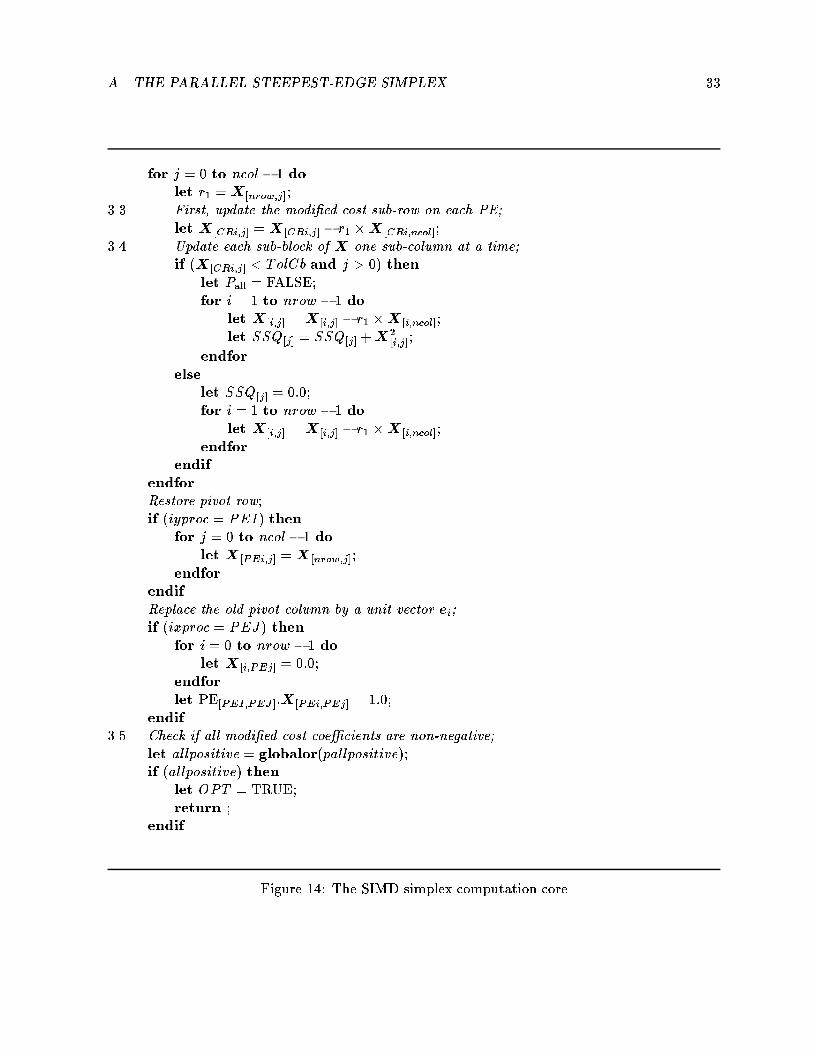
A THE PARALLEL STEEPEST-EDGE SIMPLEX 33for j = 0 to ncol � 1 dolet r1 = X [nrow;j];3.3 First, update the modi�ed cost sub-row on each PE;let X [CRi;j] = X [CRi;j] � r1 �X [CRi;ncol];3.4 Update each sub-block of X one sub-column at a time;if (X [CRi;j] < TolCb and j > 0) thenlet Pall = FALSE;for i = 1 to nrow � 1 dolet X [i;j] = X [i;j] � r1 �X [i;ncol];let SSQ[j] = SSQ[j] +X2[i;j];endforelselet SSQ[j] = 0:0;for i = 1 to nrow � 1 dolet X [i;j] = X [i;j] � r1 �X [i;ncol];endforendifendforRestore pivot row;if (iyproc = PEI) thenfor j = 0 to ncol� 1 dolet X [PEi;j] = X [nrow;j];endforendifReplace the old pivot column by a unit vector ei;if (ixproc = PEJ) thenfor i = 0 to nrow � 1 dolet X [i;PEj] = 0:0;endforlet PE[PEI;PEJ]:X[PEi;PEj] = 1:0;endif3.5 Check if all modi�ed cost coe�cients are non-negative;let allpositive = globalor(pallpositive);if (allpositive) thenlet OPT = TRUE;return ;endif Figure 14: The SIMD simplex computation core

A THE PARALLEL STEEPEST-EDGE SIMPLEX 34A.4 Search for Candidate Pivot Columns

A THE PARALLEL STEEPEST-EDGE SIMPLEX 354 Locate the best entering column PEj and its PE in PE column PEJ via Steepest-Edge;4.1 Add all partial sums SSQ and collect results in bottom row of PEs;let r2 = MAX DOUBLE;let rpj = 0;for j = 0 to ncol� 1 doif (X [CRi;j] < �TolCb) thenLogarithmic summation of all partial SSQs. Sum is stored on bottom row PEs;let d = 1;for i = 0 to log2 nyproc� 1 dolet d = 2id;let k = 2d� 1;if ((iyproc AND k) = k) thenlet SSQ[j] = xnetcN[d]:SSQ[j];endifAccount for the contribution of pivot row to SSQ+ 1:0;let SSQ[j] = SSQ[j] +X [nrow;j];4.2 Find minf� �c2jSSQ[j]g in each PE;if ((r2 > (r3 = (�X2[CRi;j]SSQ[j] ))) thenlet r2 = r3;let rpj = j;endifendforendif4.3 Locate logarithmically global min f� �c2jSSQg;if (iyproc = nyproc� 1) thenlet rPJ = ixproc;let d = 1for j = 0 to log2 nxproc� 1 dolet d = 2j ;let k = 2d� 1;if ((ixproc AND k) = k) thenlet r3 = xnetcW[d]:r2;if (r3 < r2) thenlet r2 = r3;let rPJ = xnetcW[d]:rPJ ;elselet rPJ = ixproc;endifendifendforendiflet PEJ = PE[nyproc�1;nxproc�1]:rPJ ;let PEj = PE[nyproc�1;PEJ]:rpj;Figure 15: The parallel search for the new entering pivot column

A THE PARALLEL STEEPEST-EDGE SIMPLEX 36A.5 Search for Pivot Rows

A THE PARALLEL STEEPEST-EDGE SIMPLEX 375 Locate the exiting basic column;5.1 Locate the rows with the local minimum ratio conditions in each PE in column PEJ;let allnegative = TRUE;let r2 = (r3 = MAX DOUBLE);let rpi = (rPI = 0);if (ixproc = PEJ)let rPI = iyproc;for i = 1 to nrow � 1 doif (X [i;PEj] > TolPiv and ((r3 = X [i;0]X [i;PEj] ) < r2)) thenlet rpi = i;let r2 = r3;let allnegative = FALSE;endifendfor5.2 If all elements in each sub-column PEj of all PEs in PE column PEJare negative the LP is Unbounded;if (allnegative) thenlet UNB = TRUE;return ;endif5.3 Locate the row PEi and its PE in PE row PEI with the globalminimum ratio condition;let d = 1;for i = 0 to log2 nyproc� 1 tolet d = 2id;let k = 2d� 1;if ((iyproc AND k) = k) thenlet r3 = xnetcN[d]:r2;if (r3 < r2) thenlet r2 = r3;let rPI = xnetcN[d]:rPI;elselet rPI = iyproc;endifendifendforendiflet PEI = PE[nyproc�1;PEJ]:rPI;let PEi = PE[PEI;PEJ]:rpi;endwhileFigure 16: The parallel search for the selection of the exiting basic column

B COMPUTATIONAL EXPERIMENTS TABLES 38B Computational Experiments on SPARC server 1000, MP1and MP2This section of the Appendix reports the execution time measurements on the uniprocessor work-station, the MP1, and the MP2.B.1 Computation Experiments on the Scalar WorkstationThe execution times reported in this section were measured on a Sun SPARC server 1000 work-station with 64MB of main memory. While the programwas running there was no other multiuseractivity apart from the standard background Unix processes.

B COMPUTATIONAL EXPERIMENTS TABLES 39Table 1: Average time in seconds per scalar pivot operation versus number of columns in Tableau,with 64, 256, and 512 rows M 64 256 512N Time Time Time128 0.002634 { {256 0.006810 { {512 0.021500 0.062475 {1024 0.053700 0.240000 0.4580002048 0.120900 0.641562 1.3787503072 0.240571 { {4096 0.345571 1.456670 3.5679178192 0.685909 3.300000 8.06928610240 { 4.424000 {12288 { 5.466000 {14336 { 6.516000 {16384 4.359687 8.145750 34.70428618342 { { 34.97857119456 { { 42.74000020480 { 9.974000 {21504 { { 48.40357123552 { { 53.59142924576 { 15.389000 {25600 { { 58.87642927648 { { 66.18642928672 { 24.916000 {31744 { { 80.62571432768 { 31.480000 {33792 { { 86.68428635840 { { 93.72857436864 { 35.497000 {37888 { { 99.11142939936 { { 105.54714340960 { 41.418000 {41984 { { 107.91142944032 { { 112.81714345056 { 46.081000 {46080 { { 118.94785749152 { 49.350000 {53248 { 52.619000 {57344 { 56.542500 {58368 7.767000 60.466000 {

B COMPUTATIONAL EXPERIMENTS TABLES 40Table 2: Average time in seconds per scalar pivot operation versus number of columns in Tableau,with 1024, 2048, 3072, and 4096 rowsN 1024 2048 3072 4096M Time Time Time Time2048 2.407857 { { {3072 4.958000 11.729000 { {4096 7.629000 16.195000 35.639000 {5120 { { 47.306500 67.9985006144 { 47.195000 59.078500 {8192 34.681000 74.941000 { {10240 { 102.834000 { {11264 { 118.463000 { {16384 83.721000 { { {18432 103.224286 { { {19456 106.958571 { { {20480 112.881429 { { {21504 118.429286 { { {22528 125.536429 { { {

B COMPUTATIONAL EXPERIMENTS TABLES 41B.2 Computation Experiments on MP1The execution times reported here were measured on a MP1 model of Maspar. This particularmodel consists of a 64 matrix of PEs. Each PE has 64 KB of private memory. The machine has114KB of ACU memory (scalar data memory).Table 3: Average time in seconds per SIMD pivot operation versus number of columns in Tableaux,with 64, 256, and, 512 rows, on MP1M 64 256 512N Total Comm. Total Comm. Total Comm.128 0.002642 0.001536 { { { {256 0.004159 0.002336 { { { {512 0.006099 0.003065 0.011488 0.004228 { {1024 0.013349 0.007164 0.021378 0.007463 0.031866 0.0078282048 0.025602 0.013610 0.041101 0.013928 0.061360 0.0142943072 0.037961 0.020074 { { { {4096 0.050231 0.026507 0.080679 0.026880 0.120500 0.0272668192 0.099616 0.052347 0.160386 0.052876 0.239521 0.05330016384 0.198631 0.104064 0.319017 0.104715 0.476472 0.10519718304 { { { { 0.532011 0.11736719456 { { { { 0.565326 0.12465621504 { { { { 0.624569 0.13763423552 { { { { 0.683810 0.15060925600 { { { { 0.743048 0.16358527648 { { { { 0.802277 0.17655131744 { { { { 0.920757 0.20250532768 0.397374 0.207633 0.636278 0.208394 0.954449 0.20965533792 { { { { 0.979999 0.21548135840 { { { { 1.039229 0.22844537888 { { { { 1.098472 0.24142739936 { { { { 1.157707 0.25439841984 { { { { 1.216949 0.26737344032 { { { { 1.276179 0.28034346080 0.568056 0.293575 0.901567 0.293863 1.335421 0.293319

B COMPUTATIONAL EXPERIMENTS TABLES 42Table 4: Average time in seconds per SIMD pivot operation versus number of columns in Tableaux,with 1024, 2048, 3072, and 4096 rows, on MP1M 1024 2048 3072 4096N Total Comm. Total Comm. Total Comm. Total Comm.2048 0.102507 0.015156 { { { { { {3072 0.152072 0.021726 { { { { { {4096 0.201341 0.028232 0.360847 0.029798 0.520363 0.031371 { {5120 { { 0.447960 0.036052 0.646489 0.037583 0.845172 0.0391236144 { { 0.536065 0.042526 0.773649 0.044066 1.011395 0.0455848192 0.398441 0.054267 0.712264 0.055466 1.027942 0.057000 { {10240 { { 0.888481 0.068419 { { { {12288 { { 1.064677 0.081361 { { { {14336 { { 1.240882 0.094307 { { { {16384 0.790566 0.105972 { { { { { {18304 { { { { { { {19456 0.938011 0.125437 { { { { { {20480 0.987154 0.131922 { { { { { {21504 1.036308 0.138411 { { { { { {22528 1.085451 0.144899 { { { { { {23552 1.134588 0.151377 { { { { { {

B COMPUTATIONAL EXPERIMENTS TABLES 43B.3 Computation Experiments on MP2The execution times were measured on a MP2 Maspar model. Its DPU consists of a 128 � 128PE matrix, with 64KB of private memory each. The ACU of this machine has 512KB of scalardata memory.Table 5: Average time in seconds per SIMD pivot operation versus number of columns in Tableauxwith 256, 512, 1024, and 2048 rows, on MP2M 256 512 1024 2048N Total Comm. Total Comm. Total Comm. Total Comm.512 0.002261 0.001246 { { { { { {1024 0.003807 0.001972 0.004770 0.002075 { { { {2048 0.006866 0.003407 0.008631 0.003512 0.012375 0.003856 { {4096 0.013028 0.006304 0.016421 0.006436 0.023565 0.006910 0.037089 0.0074098192 0.025567 0.012234 0.032259 0.012437 0.045760 0.012909 { {16384 0.050380 0.023937 0.063537 0.024195 0.090133 0.024890 { {23552 { { { { 0.127914 0.034731 { {32768 0.099967 0.047311 { { { { { {33792 { { 0.130009 0.049187 { { { {40960 { { { { { { 0.349355 0.06020044032 { { 0.169112 0.063890 { { { {46080 0.142947 0.067965 0.176927 0.066824 0.250995 0.068333 0.394812 0.068829

B COMPUTATIONAL EXPERIMENTS TABLES 44Table 6: Average time in seconds per SIMD pivot operation versus number of columns in Tableauxwith 3072, 6096, and, 5120 rows, on MP2M 3072 4096 5120N Total Comm. Total Comm. Total Comm.4096 0.050625 0.007905 { { { {5120 0.062538 0.009406 0.079255 0.009897 { {6144 0.074440 0.010899 0.094351 0.011397 { {16384 { { 0.244521 0.025898 { {20480 { { 0.304714 0.031777 0.368999 0.03226122528 { { 0.334803 0.034712 { {23424 { { { { 0.420567 0.03638924576 { { 0.364904 0.037659 { {26624 0.312623 0.040862 0.394994 0.040592 { {

B COMPUTATIONAL EXPERIMENTS TABLES 45B.4 Speed-Ups of Parallel over Sequential Steepest-Edge SimplexThe speed-ups reported in this subsection in a tabular form were attained by the MP2 model overthe SPARC server 1000 workstation.Table 7: Speed-ups for Tableaux with 256, 512, 1024, 3072, and, 4196 rows, on MP2M Attained Speed-upsN 256 512 1024 2048 3072 4096512 27.632 { { { { {1024 63.042 96.017 { { { {2048 93.441 159.744 194.574 { { {3072 { { 275.032 { { {4096 87.938 217.27 323.743 436.652 700.583 {5120 { { { { 753.782 859.6556144 { { { { 798.925 {8192 129.073 250.141 757.889 1040.963 { {11264 { { { 1206.848 { {16384 163.671 546.206 928.861 { { {18432 { { 1028.068 { { {19456 { 567.860 { { { {20480 { { 1013.189 { { {22528 { { 1025.532 { { {21504 { 582.544 { { { {25600 { 596.344 { { { {31744 { 626.958 { { { {32768 314.904 { { { { {35840 { 680.006 { { { {39936 { 687.733 { { { {46080 { 672.299 { { { {58368 334.330 { { { { {