A SUITABLE BAYESIAN APPROACH IN TESTING POINT NU LL

HYPOTHESIS, SOME EXAMPLES REVISITED

i:vl iguel A . Góme2- ViIlegas, Paloma. lVIaín and Luis San2

Departamento de Estadística. e Investigación Operativa

Universidad Complutense de ?vla.drid 28040 ?vla.drid , Spain

ma.gv@mat.ucm.es

Key Vlords: p- values; posterior probability; point null ; prior distribution.

ABSTRACT

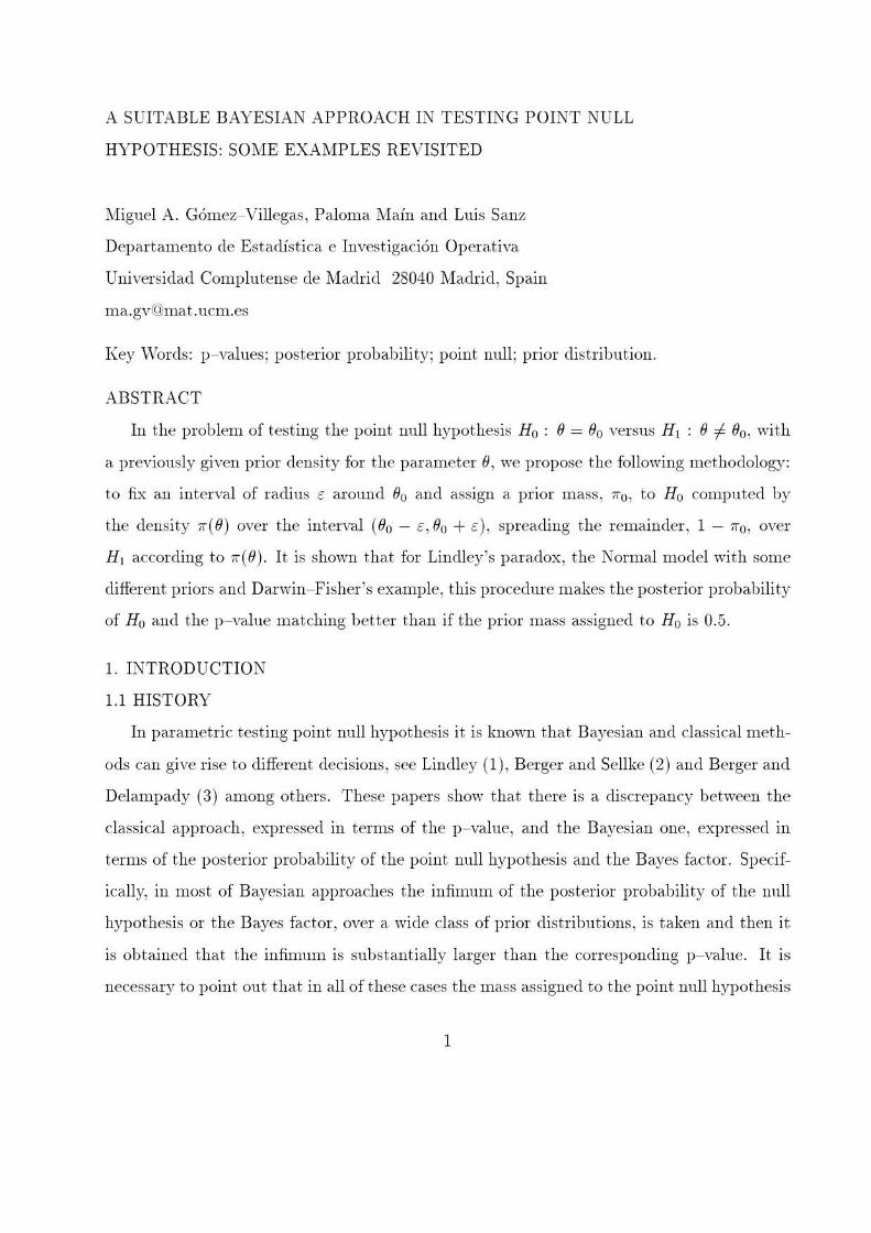
In the problem of testing the point null hypothesis Ro : 8 = 80 versus Hl : () =1 80, with

a previously given prior density for the parameter e, \Ve propose the following metbodology:

tú fix an interval of radius é around ea and assign a· prior mass, ;;0 , tú Ho computed by

tbe density iL(O) over tbe interval (00 - E, Oo + E), spreading the remainder, 1 - ;;0 , over

H1 according tú r. (O). It is shown that for Lindley's paradox, the Normal model with sorne

different priors ancI Darwin- Fisher 's exarnple, this procedure rnakes the posterior probability

of Ho and the p- vd lue rnatching better than if the prior rnass assigned to Ho is 0.5.

1. INTRODUCTION

1.1 HISTORY

In parametric testing point null hypothesis it is known tbat Bayesian and classical rneth­

ods can give ri se to different decisjons, see Lindley (1), Berger and Sellke (2) and Berger and

Ddarnpady (3) arnong otbers. These papers show that there is a discrepancy between tbe

classical approach, expressed in tenns of the p- \rd lue, and the Bayesian one, expressed in

terms of the posterior probability of the point null hypothesis and the Bayes fa,ctor. Specif­

ically, in rnost of Bayesian approa,ches the infimurn of the posterior probability of the null

hypothesis 01' the Bayes factor , over a, wide class of prior distributions, is taken and then it

is obtained tbat the infirnum is substantjally larger than the corresponding p- value. It is

necessary to point out that in all of these cases the mass assigned to the point null hypotbesis

1

is 0.5 . On the otber band, Casella. and Berger (4) show that there is no discrepancy in the

one- sided testing problem.

In most of the existing contributions a class of priors distributions is used, but our

objective is to check what happens when a single prior distribution is used. The methodology

to be proposed is the one introduced by Góme;t,- Villegas and Gómeí:l Sánche2- ?vIaní:lano (5)

and justified by Góme2- ViIlegas and San2 (6) where it is shown that the infimum of the

posterior probability can be close to the p- value when the class of priors is tbe class of all

unimodal and symmetric distributions.

Some releV"dnt references, comparing classical and Bayesian measures, in addition to those

mentioned aboye, are Pratt (7), Edwards, Lindman and Sa.V"dge (8), DeGroot (9), Bernardo

(10), Rubin (11), Mukhopadhyay and DasGupta (12), Berger, Boukai and Wang (13, 14) ,

and Oh and DasGupta (15).

In Section 1.2 we present the problem. In Section 2, tbe methodology is applied to the

Jeffreys- Lindley paradox. Section 3 contains an example with a, normal model and normal

prior. In Section 4 tbe general framework for a normal model is analy:ted and an example with

tbe Cauchy model is considered. In Section 5 we deal with the famous example of Danvin­

Fisher studied by Dickey (16). Finally, Section 6 contains some additional comments.

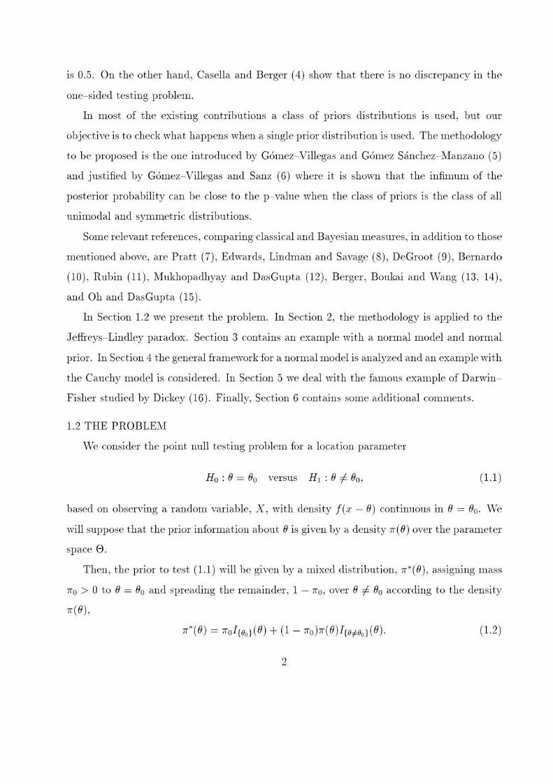
1.2 THE PROBLEM

"Ve consider the point null testing problem for a· location para meter

Ho : O = 00 versus H ] : O =/:- 00 , (1.1)

based on observing a random V"driable, X , with density 1(x - O) continuous in O = Oo. V\le

will suppose that the prior information about O is given by a density ii(O) over the parameter

space 8 .

Then, the prior to test (1.1) will be given by a· mixed distribution, ii~(O) , assigning mass

iiO > O to 8 = 00 and spreading tbe remainder , 1 - "O , over O =/:- 00 according to the density

rr(O) ,

rr ' (O) = rro I{o,¡(O) + (1 - rro)rr(O) I{o#,¡(O).

2

(1.2)

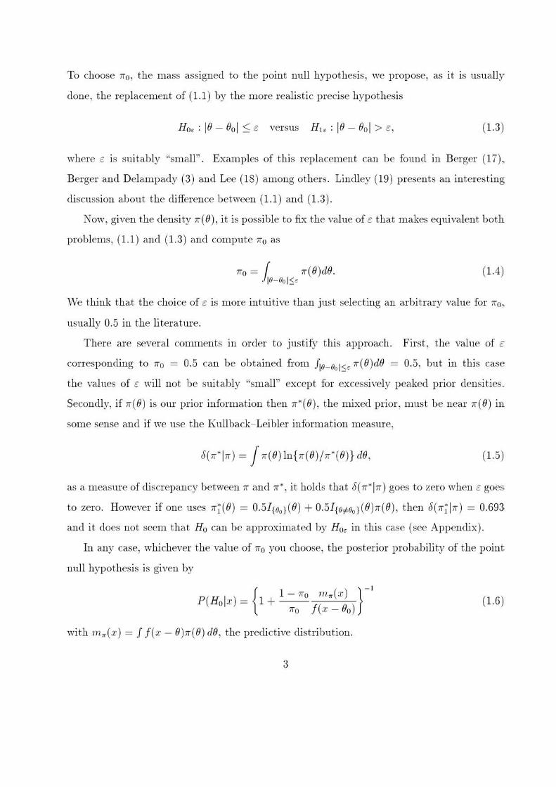
To choose iro , the mass assigned to the point null hypothesis, \Ve propose, as it is usually

done, the replacement of (1.1) by tbe more reali stic precise hypothesis

Ho~ : lO - 00 1 :S E versus Hl ~ : lO - 00 1 > E, (1.3)

wbere E is suitably "smaII" . Examples of this replacement can be found in Berger (17),

Berger and Delampady (3) and Lee (18) among others. Lindley (19) presents an interesting

discussion about tbe difference between (1.1) and (1.3).

Now, given tbe density ir (O) , it is possible to fix tbe value of E that makes equivalent both

problems, (1.1) and (1.3) and compute iro as

"o = r ,,(O)dO. Jlo-ool:::;~

(1.4)

""Te think that tbe choice of E is more intuitive tban just selecting an arbitrary value for iro,

usually 0.5 in the literature.

There are several comments in order to justif)1 this approa.ch. First, the \rdlue of €

corresponding to iro = 0.5 can be obtained from Jlo-ool:::;~ ir (O)dO = 0.5, but in this case

the values of € ",iII not be suitably "small" except for excessively peaked prior densities.

Secondly, if ir (O) is our prior infonnation tben ir~ (O), the mixed prior, must be near ir(O) in

some sense and if \Ve use the KuIIba.ck- Leibler infonnat ion measure,

5(""1") = J ,, (O) ln{,, (O)j,," (O)) dO , (1.5)

as a measure of discrepancy between ir and ir~ , it holds tbat 6( ir* l ir ) goes to %:ero when E goes

to zero. However il one uses rr¡ (O) = 0.5I{oo)(0) + 0.5I{O;iOo)(0)rr(0), then 5(rr¡ lrr ) = 0.693

and it does not seem that Ho can be approximated by Ho! in this case (see Appendix).

In any case, whichever the \rdlue of iTo you choose, the posterior probability of the point

null hypotbesis is given by

P(Hol x) = {1 + 1-"o ",.(x) } _. "o f (x - 00 )

with m·lf (x) = J f (x - O)iT(O) dO , tbe predictive distribution.

3

(1.6)

Finally, a classical l11easure of evidence aga,inst the null hypothesis, which depends on

the observd.tions, is the p- vaIue. If there exists an appropriate statistic T(X) , for exal11ple a

suflicient statistic, the p- value 1m testing (1.1 ) is given by p(,,) = P {lT(X) I > IT( x) li Bo }.

In this paper we wish to establish that the posterior probability of the point nu11 hypoth-

esis, wi th ou1' l11ethodology, is closer to the p- value than the posterior probability when the

l11ass assigned to the point null is 11"0 = 0.5, at least in the problerns \Ve have ana ly:ted. Then,

the cause oi" the discrepancy between the Bayesian and frequentist approxil11ations seel11S to

be more clear in these situations.

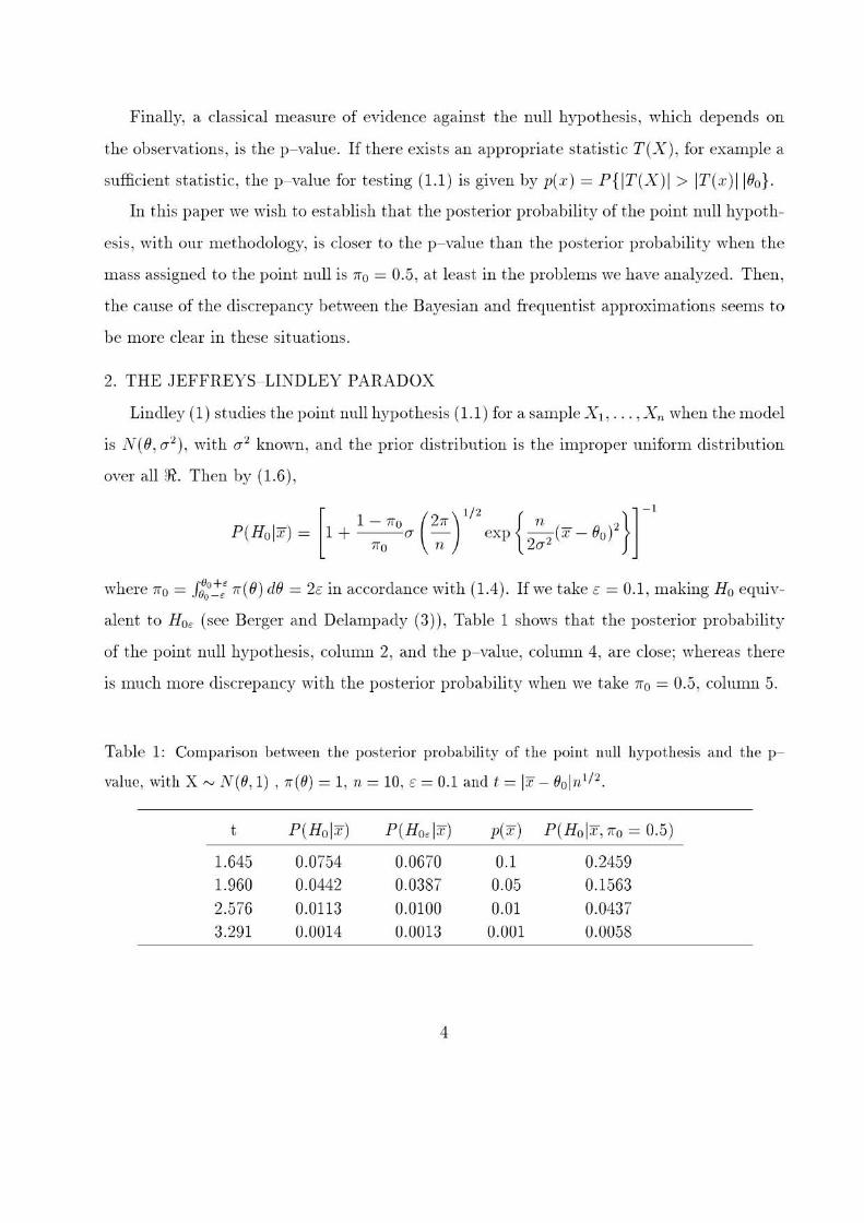
2. THE JEFFREYS- LINDLEY PARADOX

Lindley (1) studies the point null hypothesis (1.1) for a sample Xl, ... , X,¡ when the model

is N(O, (11), with (1'! knowIl , and the prior distribution is the il11proper uniform distribution

over aJl !Jl. Then by (1.6),

1 - 11"0 211" 11. 2 [ '/' j-' P(Holx) = 1 + ITo ,,( -;;-) expL", (x- Bo) }

where 11"0 = J:oO!: 11"( O) dO = 2 E in accordance with (1 .4). If we take E = 0.1, l11aking Ho equiv­

alent to Ho~ (see Berger and Delampady (3)) , Table 1 shows that the posterior probabili ty

of the point nu11 hypothesis , column 2, and the p- va.lue, column 4, are close; whereas there

is much more discrepancy with the posterior probabili ty when we take 11"0 = 0.5, column 5.

Table 1: Comparison betweell t.be posterior probability of the point llull hypothesis and the p­

value , with X '""-' N(O, 1) , 11"(0) = 1, n = 10, E = 0.1 and t = Ix _ Ooln 1f2 .

t P(Ho lx) P(Ho, lx) p(x) P(Ho lx, "o = 0.5)

1.645 0.0754 0.0670 0.1 0.2459

1.960 0.0442 0.0387 0.05 0.1563

2.576 0.01l3 0.0100 0.01 0.0437

3.291 0.0014 0.0013 0.001 0.0058

4

If \Ve take some other values of € around 0.1) the results are similar. For example) ii"

€ = 0.15 ancI t = 1.96) the posterior probability oi" Ho is 0.0734 and the posterior probabili ty

of Ho~ is P(Ho!"lx) = r~: r.(8I x) d8 = 0.0612 . On the other hand column 5, where "O = 0.5,

ean be obtained \Vith our methodology just taking € = 0.25.

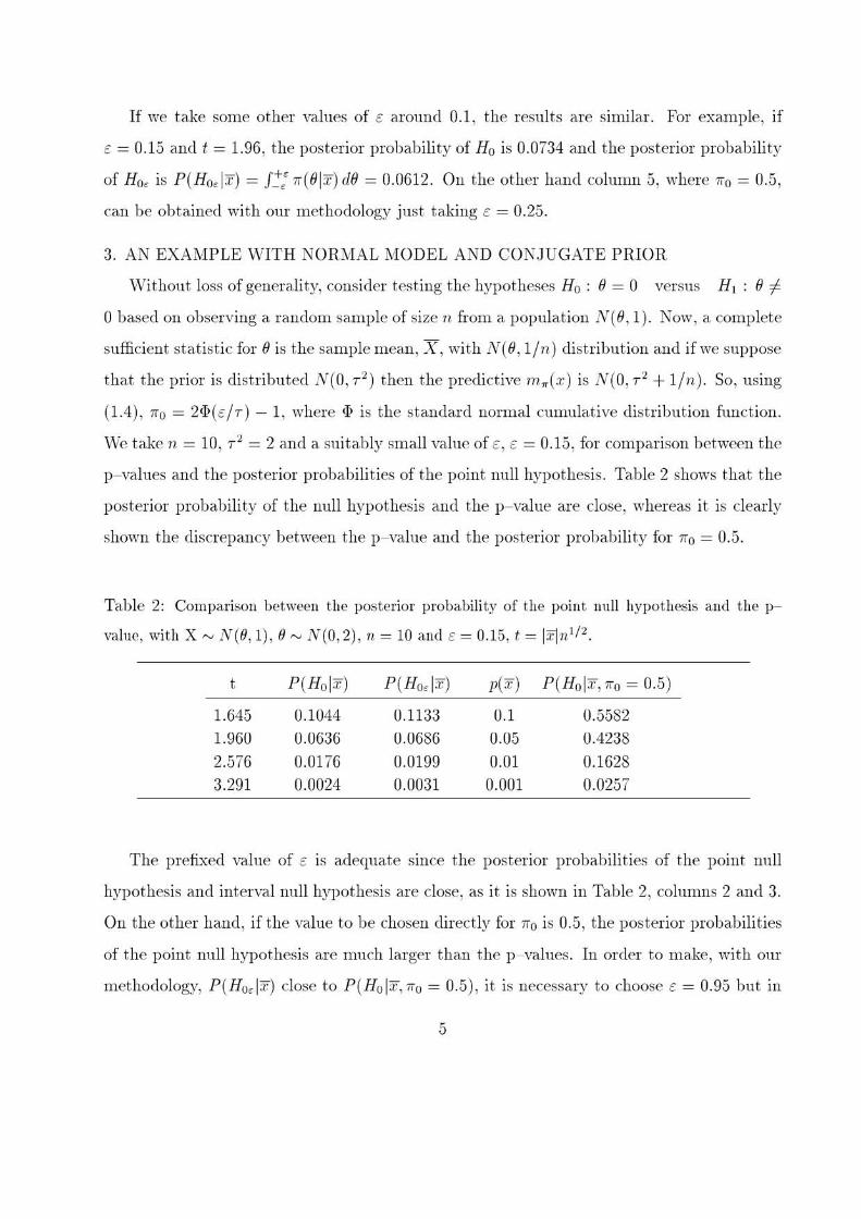
3. AN EXAMPLE WITH NORMAL MODEL AND CONJUGATE PRIOR

vVi thout 10ss of genera1ity, consider testing the hypotheses Ho : 8 = O versus H l : 8 =1

O based on observing a random sample of size n from a population N(8, 1). Now, a· complete

sufficient statistie for 8 is the samplemean, X , with N(8, 1/n) distribution and ifwe suppose

that the prior is distributed N(O, T 2) then the predictive m1t(x) is N(O, T 2 + 1/n) . So, using

(1.4), "O = 2iJ) (é/T) - 1, where iJ) is the standard normal cUlllula.tive distribution funetion.

,".re take n = 10, T 2 = 2 and a suitably sma.ll va lue of €, € = 0.15, for comparison between the

p- values and the posterior probabili ties of the point null hypothesis. Table 2 shows tha.t the

posterior probabili ty of the null hypothesis and the p- va.lue are close, whereas it is clearly

shown the discrepa.ney between the p- value and the posterior probability for Iio = 0.5.

Table 2: Comparison betweell tbe posterior probability of the point 111111 hypothesis and the p­

value, with X '"'"' N(O, 1) , O,",", N(O,2) , n = 10 and € = 0.15 , t = IXln1f2 .

t P(Ho p¡;) P(Ho, lx) ])('1') P(Ho lx, "o = 0.5)

1.645 0.1044 0.1133 0.1 0.5582

1.960 0.0636 0.0686 0.05 0.4238

2.576 0.0176 0.0199 0.01 0.1628

3.291 0.0024 0.0031 0.001 0.0257

The prefixed value of € is adequate sinee the posterior probabilities oi" the point null

hypothesis and interval null hypothesis are close, as it is shown in Ta.ble 2, columns 2 ancI 3.

On the other hand, ii" the va.lue to be ehosen direetly for Iio is 0.5, the posterior probabili t ies

of the point null hypothesis are mueh larger than the p- values. In order to make, with our

methodology, P(Ho!lx) close to P(Ho lx, ;ro = 0.5), it is necessary to choose é = 0.95 but in

5

this case E is so great that tbe point nu11 hypotbesis does not seem to be equivalent to tbe

intelYdl hypothesis.

Now, the foUowing question arises: is it possible to choose an intelYdl for E, say (E[,E2), so

tbat taking a value of E in the interval and assigning ira as in (1.4) , the posterior probability

of the point nuU hypothesis, (1.1) , and the p- value match?

Natura11y, there is a· vdlue of E, depending on the data , so that tbe p- value and tbe

posterior probability of the point nuU hypothesis are equal , but this is not our objective.

The analysis of the Table 3 shows that if E is included in the intelYdl (1/ 15, 1/7) , then the

posterior probabilities of the point null hypothesis are close to the p- values, for moderate

vdlues of the observations. Furthermore, for a· vdlue of E in (1/15, 1/7) it can be observed

in Table 3 that , coherently, the posterior probability of the point nuU hypothesis is near the

posterior probability of the interval nuU hypothesis. Thus, in this situation, the ans"'er to

the question stated aboye is affirmative.

Table 3: Values of E matching the posterior probability and the p- value, with X ,...., N(O , l) ,

(j ,...., N(O,2) and n = 10.

t E P( Ha Ix) '" p(x) P(Ho, lx)

1.645 0.143 0.1 0.1074

1.960 0.118 0.05 0.0526

2.576 0.088 0.01 0.0104

3.291 0.065 0.001 0.0010

4. COMPARISON BETWEEN THE P- VALUE AND THE POSTERlOR PROBABILITY

In this section the different properties of the posterior probability observed in previous

sections are rejoined.

Next theorem shows the beha,viour of the posterior probability of the point nuU hypoth­

esis considered as a function of tbe ObSelYdtions and E, the half length of the interval nuU

hypothesis.

6

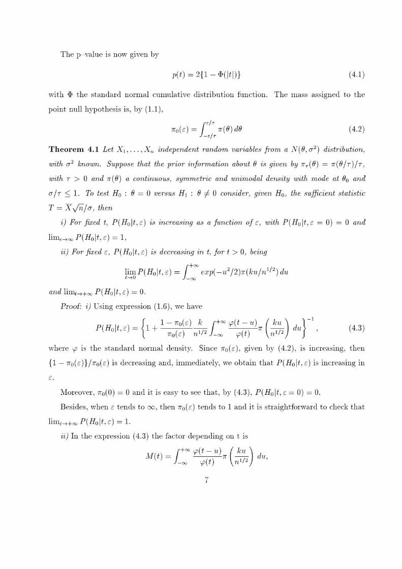
The p- value is non' given by

p(t) = 2{ 1 - <J> (lt!)} (4.1 )

with ¡P the standard normal cumulative distribution function. The rnass assigned to the

point null hypotbesis is, by (1.1),

(4.2)

T heorem 4. 1 Let Xl , ... , X n independent randorn variables fl'orn a N(O, J'J) disi1~ilndion,

with (J'J kno·w1l. Suppose that the prior information about 8 is given by ii r(O) = ii (8j r )jr ,

with T > O and ii (O) a contin-lt01ts, symmet,ic and 'Unimodal densdy ·with mode at 00 and

crjT :S 1. To test Ho : (} = O versus H! : (} :f O consider, g'iven Ho, the s-u.fjicient statistic

T = X ¡nI", then

i) F01' fixed t, P (Holt ,E) is increasing (LS a fu nction 01 E, 'UJ'ith P (Holt ,E = O) = O and

lim!....¡.oo P (Holt,E) = 1,

ii) F01' fixed E, P (Holt, E) is decreasing in t, lor t > O, being

¡+OO lim P(Holt, E) = exp(-u'/2)7r(kuln'I')du 1 ..... 0 -00

and lilll¡....¡.+oo P (Holt, E) = O.

Proof: i) Using expression (1.6), we have

{ 1 - rro(e) k ¡ +oo <p(t - u) ( kU ) }-'

P(Holt ,E) = 1 + () '1' () 7r '7'i du iiO E 11. -00 r.p t 11.

(4.3)

wbere r.p is tbe standa.rd normal density. Since Ílo(E), given by (4.2), is increasing, tben

{1 - iiO( E)} j iiO ( E) is deCl·easing and, imrnediately, we obtain that P( Ho It, E) is increasing in

E .

Moreover, iiO(O) = O and it is easy to see that , by (4.3), P (Holt, E = O) = O.

Besides, when E tends to 00, tben iiO(E) tends to 1 and it is straight forward to check tbat

limH +oo P( Ha It, ¿) = 1.

ii) In tbe expression (4 .3) the factor depending on t is

¡+OO <p(t - u) ( kU ) M (t) = () rr '7'i

-00 r.p t 11. du ,

7

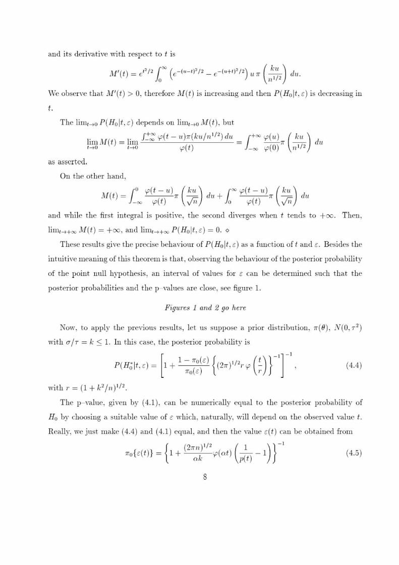
aud its derivative with respect to t is

Nf' (t) = e,2 /2 ( JO (e-(u-IF/2 _ e-( U+ I)1/2) 'Uií ( kU ) d'u. Jo '11. 1/ 2

~Vc observe t hat l\¡f'(t) > 0, thereforc 111(t) is increasing and then P(Holt, e) is dccreasing in

t.

Thc lilTl, ~o P(Holt, <) dcpcnds on lim,~o M (t), but

. " _. r~:: 'I'( t - u)r.(ku/n'/2) elu _ ¡+= 'I'(u) _ ( ku ) hmM(t) - hm ( ) - (O)" ' /2 elu 1-+0 1-+0 c.p t -00 tp n

as asserted,

On the other hand,

, ()_ ¡ O 'I'(t -U) _ ( ku ) d l ='I'(t -U) _ ( ku)d. M t- ()" ¡;: u+ ()" ¡;;; u

-00 !..p i vn o epi vn

and while the fi rst integral is positive, tIte second diverges whcn t tends to +00. Theu;

lim/-~+oo iVI(t) = +00, and lill1t-t+oo P(Holt ,e) = O. o

These rcsults give the precise behaviour of P( Holt , é) as a. function of t and é . Besides the

intuitive meaning of this theorem is that, observillg the behaviour of the posterior probabili ty

of the point null hypothesis, an interval of values for é can be detennined such that the

posterior proba.bili ties and the p- vaIues are close: see figure L

Figures 1 and 2 go here

Now, to apply the previous rcsul ts, let us suppose el prior distribution , ¡r(O), N(O, T 2)

with a-jT = k :S L In this case, t he posterior probabili ty is

P(Hñlt ,<) = [1 + 1 :o~:~e) { (2" )' /2,'I' U)} -'j -' (4 .4 )

with,. = (1 + k 2¡,,) ,/'.

T he p- value, givcn by (4.1), can be numcrically equal to tho posterior probability of

Ho by choosing a suitable value of e which, nat urally, wiII depend on thc observed vaIue t.

Really, wejust make (4.4) and (4.1) cqual, and then the value e(t) can be obtained fro111

{ (2",,) ' /2 (1 ) }-' Too {e(t)) = 1 + k 'I'("t) -() - 1

0' .. P t (4 .5)

8

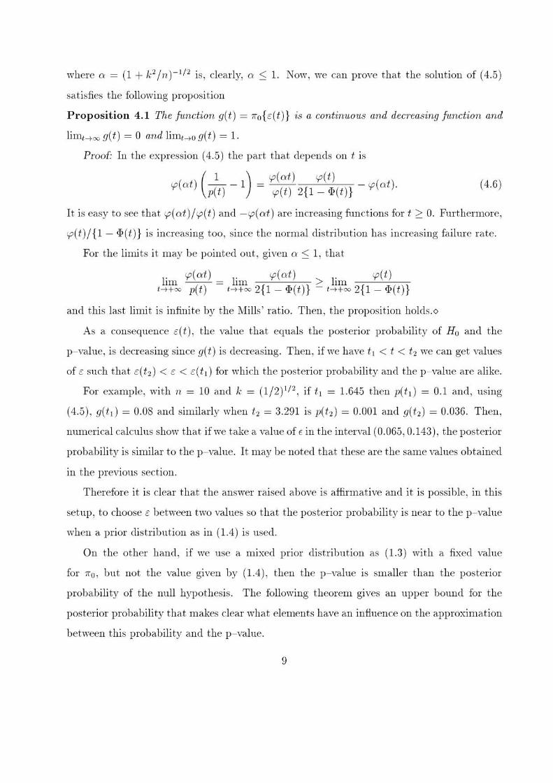
where O' = (1 + k2jn)-I/Z is, clearly, Ú'::S: 1. Now, we can prove tha.t the solution of (4.5)

satisfies the following proposition

P ropositio n 4. 1 The fundíon g(t) = 11"o{E(t )} is a continnous and decreasing jnnction and

lim¡ -+oog(t) = O and lim¡.-+og(t) = l.

Proof: In the expression (4 .5) the part that depends on t is

( 1 ) <p(al ) '1'(1)

'1'(01 ) 1'(1) - 1 = '1'(1) 2{1 - <1> (1 )) - <p(al ). (4.6)

It is easy to see that r.p(<..ti)jr.p(t) and -r.p(o-t ) are increasing functions for t 2: O. Furthermore,

r.p( t)j {1 - 1Jl ( t)} is increasing too, since the normal distriblltion has increasing failure rateo

For the limi ts it ma.y be pointed out , given o- ::s: 1, that

lim <p(al) = lim <p(al) , ~+oo p(l) , ~+oo 2{l - <I> (I)}

> lim '1'(1) - , ~+oo 2{1 - <I> (I)}

ancI this Iast limi t is infini te by the Mills' ratio. Then, the proposi tion hoIds.<>

As a. consequence E(t), the value that equals the posterior probabili ty of R o a.nd the

p- vaIue, is deo·easing since g(t) is den·easing. Then, ifwe have tI < t < t2 we can get va lues

of é such tha.t é(t2) < é < E(tl) fOl" which the posterior probability and the p- va lue are alike.

For exarnple, with n = 10 and k = (1/ 2) 1/2, if tI = 1.645 then p(t l ) = 0.1 and, using

(4.5), g(l') = 0.08 and similarly when 12 = 3.291 is ])(12 ) = 0.001 and g(12 ) = 0.036. Then,

numericaI calcuIus sho\\' that if \Ve take a value of é in the interval (0.065, 0.143), the posterior

probability is similar to the p- vaIue. It may be noted that these are the same "aIues obtained

in the previous section.

Therefore it is clear that the answer raised aboye is affirmative ancI it is possibIe, in this

setup , to choose E between two vaIues so that the posterior probabiIity is near to the p- vaIue

when a. prior distri bution as in (1.4) is used.

On the other hand, if \Ve use a mixed pnor distribution as (1.3) wi tb a fixed value

for iro, but not the vaIue given by (1.4), then the p- value is smaUer than the posterior

probabili ty oi" the null hypothesis. The following theorem gives an llPper bound for the

posterior proba.bili ty that males clear wha.t eIements have an inflllence on the approxima.tion

between this probability and the p- vaIue.

9

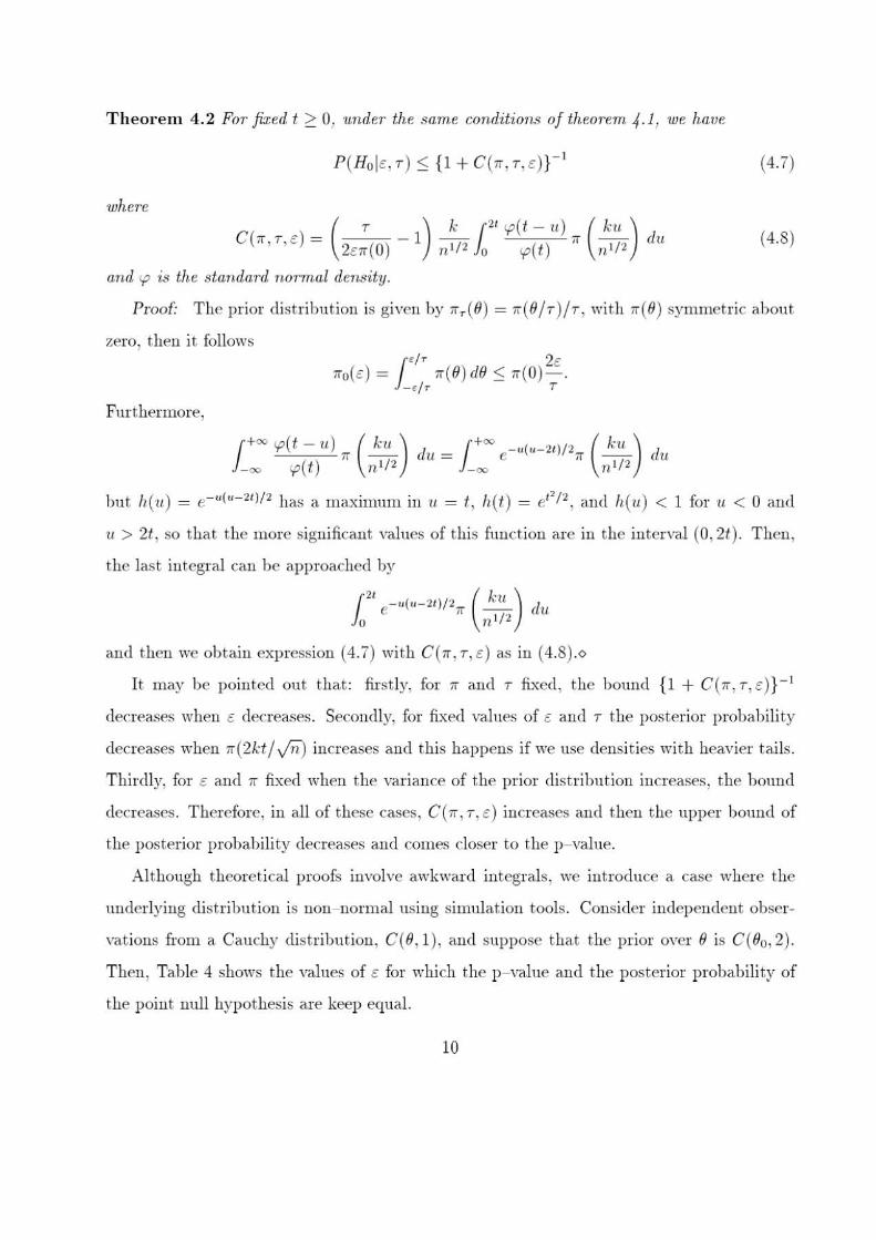
Theore m 4.2 For fixed t 2: O; under the same conditions 01 theorem 4-11 we have

P(Ho le, T) :'O (1+ G(rr , T, eW' (4 7)

'Where

G(rr , . ,e) = Ce:(o) -1) ,,712 f ~~~)u) rr (,;'~2 ) du (4 .8)

and tp is the standm'd n01'1nal densdy.

Proo¡' The prior distribu tion is given by rr r(9) = rr(B/T)/T) with rr (9) synuuetric ahout

zero¡ then it follows

J' I' 2e rro (e) = rr(O) dO :'O rr(O)-.

_~/r T Furthermore,

J+OO ~(t - u) _ ( ku ) d _ J+OO - "1"- 211/2 ( kU ) d.

" -- lt- e rr -- " -00 tp(t ) 11. 1/ 2 -00 n l / 2

but h(u) = e-u( u- 2t)/2 has a maximum in -u = t ) h(t) = el ' / 2 , and h(-u) < 1 fol' -u < O amI

1t > 2t, so that the more significant values of this function are in the interva l (O, 2t) . Then,

the last integral can be approa,chcd by

{ 21 e- u(u -21)/2 rr ( ku ) du Jo 11. 1/ 2

and thcn weobtain exprcssion (4 .7) wi th C(rr , T) é) as in (4.8) .0

It lUay be pointed out that : firstly, fOl" rr and T fixcd , the bound (l + C(rr,T, é)} - 1

deueases when é decreases. SecondIy, for fixed vaIues of é and T the posterior probabili ty

deCl·eases ,,,hen rr(2kt / Jn) increases and this happens if we use dellsities with heavier tails.

ThirdIy, fOl" é and íi fi..xed when the wU"iance of the prior distribution increases, the bound

decreases. Therefore, in a.ll of thesc cases, C( ir 1 T , é) increases and thcn the uppcr bound of

the posterior probability decreases amI comes dosel' to the p- va lue.

Although theoretical proofs involve awkwanl illtegrals, we introduce a case where the

undcrlying distribution is non- normal using simulation tools. Considcr independcnt obse1'­

vatiolls from a. Cauchy dist ribu tion , C(O, l ), and suppose that the prior over B is C(Oo,2).

Then, Table 4 shows the vaIues of é for which the p- value amI the posterior probability of

the point null hypothesis are keep equal.

ID

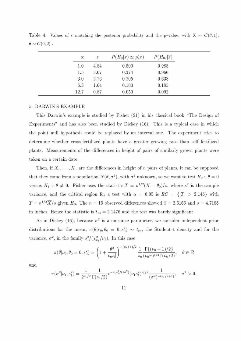
Table 4: Va lues of é matching the posterior probahility and the p- value, with X '" C(O, l) ,

o ~ C(O, 2) .

x e P(Holx) "" p(x) P(Ho,lx)

1.0 4.84 0.500 0.988

15 3.67 0.374 0.966

30 2.76 0.205 0638

63 1.64 0.100 0.185 12.7 0.87 0.050 0.092

5. DARWIN·S EXAMPLE

This Danvin's example is studied by Fisher (21 ) in his classical book "The Design of

Expel'iments': and has also been studied by Dickey (16). This is a typical case in which

t he point null hypothesis could be replaced by an interval one. The experiment tries to

determine whcther cross-fcrtilizcd plants have a greater gl'Owing rate than self- fer tilized

plants. Measurements of the diffel'enccs in hcight of pai1's of similarly grown plants were

taken on a cer tain date.

Then, if Xl , .. . , X " a,re the differences in height of 11 pai rs of plants , it can be supposed

that they come fl'Om a population N(8, 0'1) , with 0'1 unkno\Vn, so we want to test Ho : fJ = O

versus Hl fJ f. O. Fisher uses the sta tistic T = 11. [/2( X - fJo)/ s, where 3 2 is t he sample

variance, and the cri tical region for a test with O' = 0.05 is Re = { IT I > 2.145} with

T = n 1/ 2X fs given Ha. The n = 15 observed differences showed x = 2.6166 and 3 = 4.7188

in inches. Hel1 ce the statistic is t l ,[ = 2. 1476 and the test \Vas ba.rel)' significant.

As in Dickey (16), because 0''1. is a. nuisance parametel' , \Ve consider independent prior

distribu tions fol' the mean, ;r(8Iva, fJa = 0,3&) "" t/.'t), the Student- t dcnsity and for the

va riallce, 0'2 , in the famil)' 3UL\;~Jv¡). In th is case

.. (Olvo ,Oo = O,s;) =

ancl

11

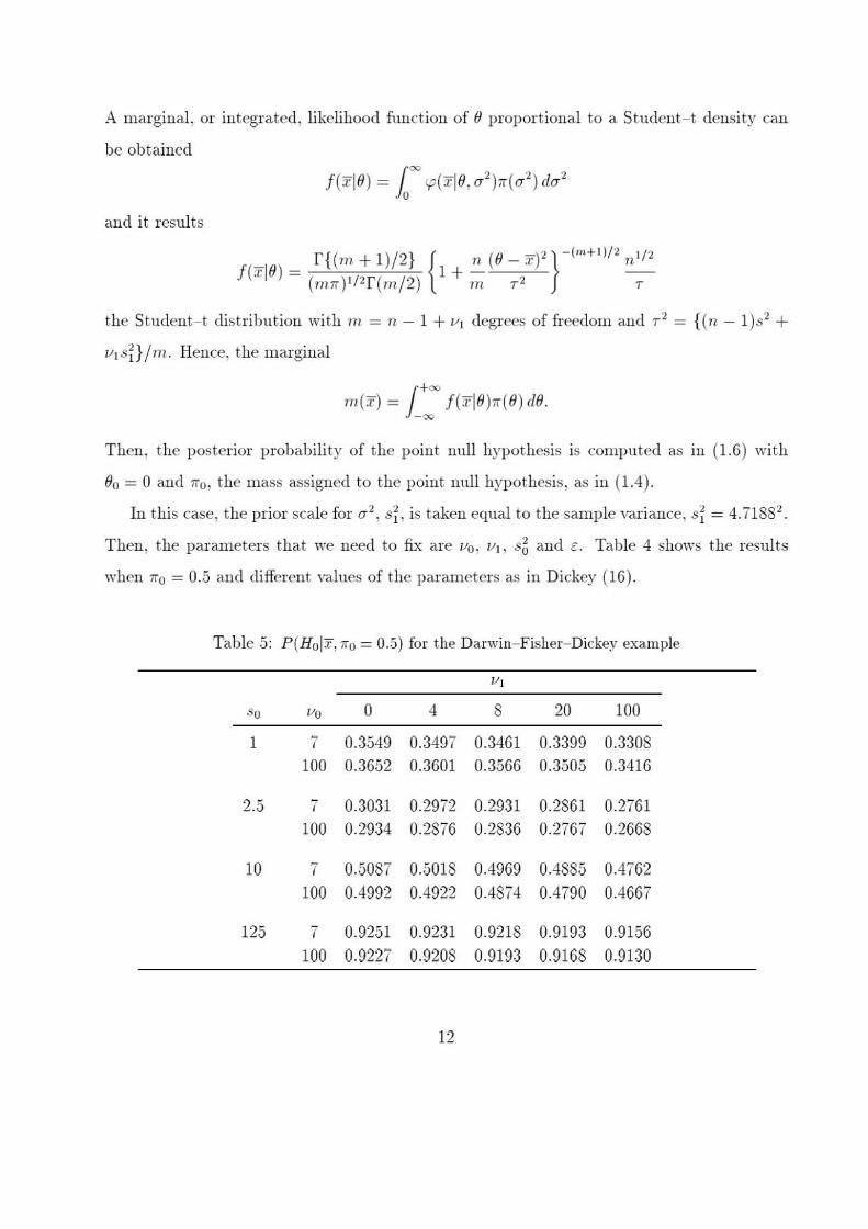
A marginal , 0 1' integratcd, likelihood function of (J proportional to a. Student- t dcnsity can

be obtained

ancl it results

f -1" r{(m + 1)/2) { n (O - x)2 }-(,.,+IJ/2 n '/2

( tu)- 1+- -. - (m rr )1/2r(m/2) m T2 T

the Student-t distribution with m = n - 1 + V I degrces of frecdom and T'1 = {(n - l )s'1 + vl sD/m. Hence, the marginal

¡+= 711(:/') = _= f(xIO)¡;(O) dO.

Then, the posterior probabili ty of the point null hypothes is is computed as in (1.6) wi th

(Jo = O and ¡ro, the mass assigned to thc point null hypothcsis, as in (1.4) .

In this case, the prior scale for (j '1, si, is taken equaJ to the sample vaúance, si = 4.71881.

Then, the parameters that we need to fix are Vo , V I , s& and € . Table 4 shows the results

when "O = 0.5 and different va lues of the parametcrs as in Dickcy (16).

Table 5: P(Ho lx, ITo = 0.5 ) for the Darwin- Fisher- Dickey example

VI

So Vo O 4 8 20 100

1 7 0.3549 0.3497 0.3461 0.3399 0.3308

100 0.3652 0.3601 0.3566 0.3505 0.3416

2.5 7 0.3031 0.2972 0.2931 0.2861 0.2761

100 0.2934 02876 0.2836 0.2767 0.2668

10 7 0.5087 0501 8 0.4969 0.4885 0.4762

100 0.4992 0.4922 0.4874 0.4790 0.4667

125 7 0.9251 09231 0.9218 0.9193 0.9156

100 0.9227 09208 0.9193 0.9168 0.9130

12

For a, fixed 30, the posterior probabilities are robust with respect to the shape va of the

prior density of O and to the degree V1 of the prior distribution of (1'2 . Moreover , it can

be noted tha.t the posterior probability of the point null hypothesis tends to one when the

conditional prior di spersion, 36, of O increases. That is, we can get a· posterior probability

close to one just increasing 36, but it means tha.t if the prior distribution tends to give

less knowledge about O then the posterior probability of the point null hypothesis becomes

grea.ter. It does not look reasonable.

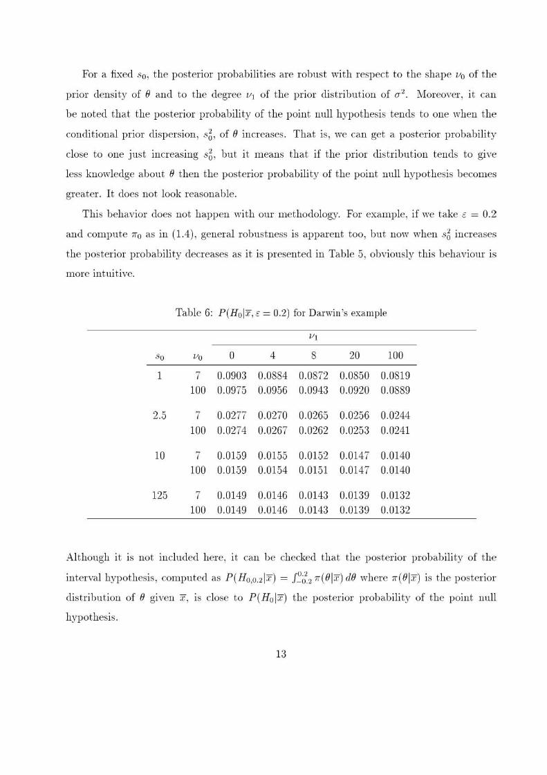
This behavior does not bappen with our methodology. For example, if we take é = 0.2

and compute ;;0 as in (1.4), general robustness is apparent too, but no'" when 36 increases

the posterior probability decreases as it is presented in Table 5, obviously this beha,viour is

more intuitive.

Table 6; P(Holx, é = 0.2) rOl" Danvin's example

"1

So Vo o 4 8 20 100

1 7 0.0903 0.0884 0.0872 0.0850 0.0819 100 0.0975 0.0956 0.0943 0.0920 0.0889

2.5 7 0.0277 0.0270 0.0265 0.0256 0.0244 100 0.0274 0.0267 0.0262 0.0253 0.0241

10 7 0.0159 0.0155 0.0152 0.0147 0.0140 100 0.0159 0.0154 0.0151 0.0147 0.0140

125 7 0.0149 0.0146 0.0143 0.0139 0.0132 100 0.0149 0.0146 0.0143 0.0139 0.0132

Although it is not included bere, it can be checked tha.t tbe posterior probability of tbe

interval hypothesis, computed as P(HO,O.2Ix) = J~o~21r (O lx) dO where 1r (Olx) is tbe posterior

distribution of O given x, is close to P(Ho lx) tbe posterior probability of tbe point null

hypothesis.

13

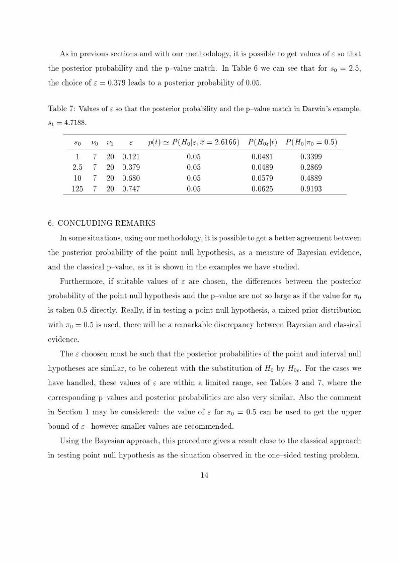
As in previous sections and with our methodology, it is possible to get vdlues of E so that

the posterior probability and the p- \rdlue match. In Table 6 we can see that for So = 2.5,

the choice of E = 0.379 leads to a posterior probability of 0.05.

Table 7: Values of E so that the posterior probability and the p- value match in Oanvin 's example,

S l = 4.7188.

So Vo VI E p(t) "" P(Ho IE, X= 2.6166) P(Ho, lt) P(Ho lrro = 0.5)

1 7 20 0.121 0.05 0.0481 0.3399

2.5 7 20 0.379 0.05 0.0489 0.2869

10 7 20 0.680 0.05 0.0579 0.4889

125 7 20 0.747 0.05 0.0625 0.9193

6. CONCLUDING REMARKS

In some situations, using our methodology, it is possible to get a better agreement between

the posterior probability of the point nuII hypothesis, as a, measure of Bayesian evidence,

ancI the classical p- value, as it is shown in the examples we ha,ve studied.

Furthermore, if suitable values of E are chosen, the differences between the posterior

probability of the point null hypothesis and the p- vdlue are not so large as if the value for ira

is taken 0.5 directly. Really, if in testing a point null hypothesis, a· mixed prior distribution

with ira = 0.5 is used , there wiII be a, remarkable discrepancy between Bayesian ancI classical

evidence.

The E choosen must be such that the posterior probabilities of the point ancI intelYdl nuII

hypotheses are similar, to be coherent with the substitution of Ha by Ho~ . For the cases we

have handled, these vdlues of E are within a limited range, see Tables 3 and 7, where the

corresponding p- values and posterior probabilities are also very similar. Also the comment

in Section 1 may be considered: the vdlue of E for ira = 0.5 can be used to get the uppel·

bound of E- however smaIIer values are recommended.

Using the Bayesian approach, this procedure gives a result close to the classicaI approadl

in testing point nuII hypothesis as the situation observed in the one- sided testing problem.

14

APP ENDIX

Thcre is a. problcm in using (1.5) as a measurc of discrepancy between 7i and 7r~ because

rr(B) is a dCllsity hut ,,"(8) is not a density. \ 'Ve can SOl't out thc pl'oblcm considcl'ing two

mea sures on (n , (B)"R. )' Fol' all .4 in tIte Bore! u - field \Ve define:

1'(04) = j' rr(O)d>' (O), A

{ { rro + (1 - rro)/,(A) .ud 1,-(04 ) = j , rr-(O)d>' (O) =

A (1 - rro),,(A)

if 80 E A,

if 80 E AC

Tho measurc ¡.t(A) is ol'iginated by thc density rr (B) and 11'" (A) by ¡¡'"(in, with "O given by

(1.4) and ). thc Lebcsguc l1lcasurc.

It is casy tú prove tha.t {l. is absolutcly continuous with respcct tú ¡.t" (¡.t « 11-), so it exits

clp,/ dI-'- l the Radon- Nikodym derivative of tt wit h respect tú ¡t'" . Besides, it is straightfonvard

tú see that

,.1" (8) = { o 1 d,,-1 -ñO

if 8 = Bo:

ir o '" 00

(A.l)

No"" using tha t 1-1. « 1-1,. , \Ve can define the discrepal1cy between 1-1' and It- as Ó(IL·I /J) =

j,,(lu(dl,.j dl,'-))dll. Theu, by (A.l), we have 0(/'-1,,) = - ln(1 - rro).

ACKNOWLEDGEMENT S

\~íe are very gl'ateful tú t he Edi tor and two 8110nymous rcfcl'ces fol' their helpful commcnts

and valuable suggestions on a previous version ofthe papel'. This research has been sponsol'cd

by DGES (Spaiu) tlnder grant PB- 9S- 0797.

BIBLIOGRAPHY

(1) Lin(lle)', D.V. A sta.tistical paradox. Biometrika, 1957, .f.f, 187- 192.

(2) Berger , J .0. ; Sellkc, T. Testing a point null hyphoteses: The irrcconciliabili ty oC p- va.lues

and cvidencc, (with discllssion). J. Amer. Statist. Assoc. ) 1987, 82, 112- 139.

(3) Bcrgcl', J .O. ; Delampady, M. Testing precise hyphoteses, (with discussion). Statistical

Science, 198 7, 2(3), 317- 352.

15

(4) Casella, G.; Berger, R.L. Reconciling Bayesian and frequenti st evidence in the one-sided

testing problem, (with discussion) . .l . Amer. Statist. Assoc. 1987, 82, 106- 135.

(5) Góme;t,- Villegas, i\LA.; Góme;t, Sánche%:-Man%:ano, E. Bayes factor in testing precise hy­

photeses. Commun. Statist. - Theory Meth. , 1992, 21, 1707-1715.

(6) Góme;t,- Villegas, M.A .; Sam;, L. Reconciling Bayesian and frequenti st evidence in the

point null testing problem. Test, 1998, 7(1) , 207- 216 .

(7) Pratt , J .vV. Bayesian interpretation of standard inference statements . .l . Roy. Statist .

SoC. B, 1965, 27, 169- 203

(8) Edwards, "V. L.; Lindman, H.; Sa.vdge, L . .l . Bayesian StatisticaI Inference for Psycho-

10gicaI Research. Psychol. Rev. , 1963, 70, 193- 248. Reprinted in Rob"nstness 01 Bayesian

Analysis (J .B. Kadane, ed.) Amsterdam: North- Holland, 1984, 1- 62.

(9) DeGroot , M.H. Doing what comes naturally: Interpreting a tail area. as a posterior

probability or as a, likelihood ratio. J. Amer. Statist. Assoc. , 1973, 68, 966- 969.

(10) Bernardo, .l .M. A Bayesian analysis of classicaI hypothesis testing in: .l .M. Bernardo,

M.H. DeGroot , D.V. Lindley and A.F .lVI. Smith, eds., Bayesian Statistics (University Press,

Valencia') , 1980, pp. 605- 647 (with discussion) .

(11) Rubin , D.B . Bayesianly justifiable and relevant frequency calculations for the applied

statiscian. Ann. Statist ., 1984, 12, 1151- 1172

(12) Mukhopadhyay, S.; DasGupta , A. Unifonn approximation of Bayes solutions and pos­

teriors: Frequentistly \rdlid Bayes inference. Statistics ancI Decisions, 1997, 15, 51- 73.

(13) Berger, J .O.; Boukai , B.; "Vang, Y. Unified frequentist and Bayesian testing of a precise

hypothesis. Satistical Science, 1997, 12(3) , 133- 160.

(14) Berger, J .O.; Boukai, B.; vVang, Y. Simultaneous Bayesian- Frequentist sequential test­

ing of nested hypothesis. Biometrika, 1999, 86, 79- 92.

16

(15) Oh, H.S.; DasGupta , A. Comparison of tbe p- V"d lue and posterior probability. J . of

Statist. Planning and Inference, 1999, 76, 93- 107

(16) Dickey, .L M. Is tbe tail area. useful as an approxirnate Bayes factor? .l. Ame!". Stat ist .

Assoc. , 1977, 72, 138- 142.

(17) Berger, .l.O. Statistical Decision TheoTy and Bayesian Analysis, Springer Verlag, New

York, 1985.

(18) Lee, P.?vI. Bayesian Statistics: An Introd1J.ction, Charles Griffin , London, 1994.

(19) Lindley, D.V. Statistical inference concerning Hardy-\>Veinberg equilibrium. Bayesian

Statistics 3, .l j\lI. Bernardo et al. Oxford University Press. 1988, 307- 326.

(20) Góme,,- Vi11egas, i'vI.A.; San", L. é-contaminated priors in testing point nu11 hypotbesis:

a procedure to determine the prior probability. Statist. and Probab. Lett. , 2000, 47(1)

53- 60.

(21) Fisher , R.A. Statistical Methods and Sci entific Inference. Edinburgh: Oliver and Boyd,

1956 / 1973. R.eprinted in 1990 witbin Statistical l\,IIetbods, Experimental Design and

Scientific Inference (J.M . Bennet , ed.) Oxford: University Press.

17