Journal of

Actuator NetworksSensor and

Article

A Study on Sensor System Latency in VR Motion Sickness

Ripan Kumar Kundu 1,*, Akhlaqur Rahman 2 and Shuva Paul 3

�����������������

Citation: Kundu, R.K.; Rahman, A.;

Paul, S. A Study on Sensor System

Latency in VR Motion Sickness. J.

Sens. Actuator Netw. 2021, 10, 53.

https://doi.org/10.3390/

jsan10030053

Academic Editor: Ugo Fiore

Received: 10 April 2021

Accepted: 13 July 2021

Published: 6 August 2021

Publisher’s Note: MDPI stays neutral

with regard to jurisdictional claims in

published maps and institutional affil-

iations.

Copyright: © 2021 by the authors.

Licensee MDPI, Basel, Switzerland.

This article is an open access article

distributed under the terms and

conditions of the Creative Commons

Attribution (CC BY) license (https://

creativecommons.org/licenses/by/

4.0/).

1 Faculty of Computer Science & Electrical Engineering, University of Rostock, Albert Einstein Str. 2,18059 Rostock, Germany

2 School of Industrial Automation, Engineering Institute of Technology, Melbourne, VIC 3000, Australia;akhlaqur.rahman@eit.edu.au

3 School of Electrical and Computer Engineering, Georgia Institute of Technology, Atlanta, GA 30332, USA;spaul94@gatech.edu

* Correspondence: ripan.kundu@uni-rostock.de

Abstract: One of the most frequent technical factors affecting Virtual Reality (VR) performance andcausing motion sickness is system latency. In this paper, we adopted predictive algorithms (i.e.,Dead Reckoning, Kalman Filtering, and Deep Learning algorithms) to reduce the system latency.Cubic, quadratic, and linear functions are used to predict and curve fitting for the Dead Reckoningand Kalman Filtering algorithms. We propose a time series-based LSTM (long short-term memory),Bidirectional LSTM, and Convolutional LSTM to predict the head and body motion and reduce themotion to photon latency in VR devices. The error between the predicted data and the actual datais compared for statistical methods and deep learning techniques. The Kalman Filtering method issuitable for predicting since it is quicker to predict; however, the error is relatively high. However,the error property is good for the Dead Reckoning algorithm, even though the curve fitting is notsatisfactory compared to Kalman Filtering. To overcome this poor performance, we adopted deep-learning-based LSTM for prediction. The LSTM showed improved performance when compared tothe Dead Reckoning and Kalman Filtering algorithm. The simulation results suggest that the deeplearning techniques outperformed the statistical methods in terms of error comparison. Overall,Convolutional LSTM outperformed the other deep learning techniques (much better than LSTM andBidirectional LSTM) in terms of error.

Keywords: cross-correlation; dead-reckoning; deep learning; kalman filtering; latency; LSTM; predic-tive tracking; sensors; Virtual Reality

1. Introduction

In an ever-changing world seeking regular technological advancement, Virtual Realityhas been proven to play an imperative role in the further advancement of scientific progressin many sectors of our lives. Virtual Reality (VR) refers to a computer-simulated environ-ment that produces a sensible and intuitive 3D environment that clients can understandthrough a head-mounted display (HMD). However, the assessment of VR has brought up awell-known issue of many users suffering from motion sickness (MS), which is also knownas simulation sickness or visually induced motion sickness (VIMS). In addition, motionsickness can be referred to as a mal-adaptation syndrome when exposed to real and/orapparent motion [1]. The signs or symptoms of motion sickness include nausea, excessivesalivation, cold sweating, and drowsiness [2]. MS is categorized by actual motion on land,sea, and air, [1]. The cause of motion sickness is described in multiple theories, i.e., thesensory conflict theory [3], evolutionary/poison theory, postural instability theory, eyemovement theory, and rest-frame hypothesis theory [4]. These theories argue for differentcausal factors describing the effects of mal-adaptation while sensing real or perceivedmotion.

The most common causal theory of MS, the Sensory Conflict Theory, was first proposedin 1975 [1]. According to the Sensory Conflict Theory, the visual systems generate the sensory

J. Sens. Actuator Netw. 2021, 10, 53. https://doi.org/10.3390/jsan10030053 https://www.mdpi.com/journal/jsan

J. Sens. Actuator Netw. 2021, 10, 53 2 of 18

inputs to the brain. The vestibular systems are different sensations experienced at differenttimes, which cause MS. The perception of visual change (such as time delays found inthe Head-Mounted Displays (HMDs) or Virtual environments (VEs)) causes a situationwhere the observing visual images are different from the user learned and mapped duringthe development phase. These are possible sources of sensory conflict [4]. These effects ofsensory conflict frequently result in MS. Additionally, the optical and temporal distortionsare also considered as sources of MS. These distortions occur due to the change of thedesired inputs of the visual and vestibular systems. In [4], the term “simulator sickness” (ss)method was also used to describe MS. Researchers measured simulator sickness estimatesand reports about MS symptoms during simulator and VE exposure [5]. Some technicalfactors cause MS. For example, a large field of view (FOV) can increase MS.

In addition to the FOV, other factors include latency, tracking accuracy, calibration,tracking precision, lack of positional tracking, judder, refresh rate, display response time,and persistence, all of which can be considered reasons for MS. In addition, other individualfactors cause MS. For instance, lateral movement, expectations, experience with VR, think-ing about sickness, and mental models can cause MS. Further factors include: instructionfor how to put on the HMD correctly, sense of balance, Read–Write (RW) experience withthe task (the less, the better) [3].

Concurrent to VR, application of machine learning and deep learning methods havealso become increasingly common in different sectors, including power grid security [6],energy management [7], weather impact analysis on critical infrastructures [8], game theoryanalysis [9,10], robotics [11], medical diagnosis [12,13], and agriculture advisory [14], etc.Deep learning methods for human body prediction have made significant progress.

In [15,16] different deep recurrent neural networks (RNN) and Long short-term mem-ory (LSTM) models were proposed to predict the human future trajectories. However,their models attempted to learn general human movement from a large collection of im-ages/videos. The LSTM model, which can learn generic human movement and predictfuture trajectories, was used in [15]. The authors proposed a Social-LSTM that predictedpedestrian trajectories more accurately than existing algorithms, which was applied ontwo publicly available datasets.

In [16], the authors proposed a single Gated Recurrent Unit (GRU) LSTM insteadof usual multi-layer LSTM architectures for short-term motion prediction using humanskeletal data to learn human kinematics. These models are complicated since they aredesigned to learn patterns from a set of skeletal data and predict up to 80 millisecondsahead of time. However, head motion prediction in six degrees of freedom (6DoF) is moredifficult than in 360-degree video (3DoF) since both the location and viewing direction canchange at any time, and users have a much wider virtual space to explore [17,18].

Thus, the resulting precision of the predicted location is much lower than what isneeded for pre-rendering in the VR scenarios. The most difficult aspect of this particularmethod is to meet the ultra-low latency requirements since streaming 360-degree video canconsume quite a lot of bandwidth. Good VR user experiences essentially require ultra-lowlatency (less than 20 ms) [19].

Motivated by the aforementioned latency-related challenges, in this paper, we studyVR devices to predict head and body motions to meet the ultra-low latency require-ments [20]. As we know, latency issues disrupt the VR device performance when auser portraits the captured motion on display. One approach is to perform predictivepre-rendering using the edge device/computer and then to stream the expected view toHMD (as long as we can predict the users’ head and body movement/motion for theimmediate future) [21].

This paper’s contributions include investigating the performance of the position pre-diction using statistical and deep-learning-based prediction techniques (i.e., Dead Reckon-ing, Kalman Filtering, deep-learning-based long short-term memory (LSTM), BidirectionalLSTM, and Convolutional LSTM). Initially, we review the theories related to motion sick-ness (MS) in Section 2. Then, the technical factors causing the MS in VR and Augmented

J. Sens. Actuator Netw. 2021, 10, 53 3 of 18

Reality (AR) devices are discussed (see Section 2). In Section 3, we discuss the commonpredictive algorithms for predictive tracking.

Later, the most critical factor, called latency, is considered for the simulation. In orderto reduce the system delay or latency, we investigate the performance of Dead Reckoningand Kalman Filtering at first. Following that, we deploy deep-learning-based approachesLSTM, Bidirectional LSTM, and Convolutional LSTM (see Section 4). Finally, we concludethis study by analyzing and comparing the error performances between these statisticallearning and deep-learning-based methods in Section 5.

2. Technical Factors Related to the Motion Sickness in Virtual Environment

In this section, a few technical factors involved in motion sickness in a virtual environ-ment are discussed, such as field of view, latency, sensors, rendering, and display

2.1. Motion Sickness (MS) Incidence, Symptoms, and Theories

The word “Cybersickness” does not refer to a disease or a pathological state, rather toa typical physiological response that comes from an abnormal stimulus [22]. Cybersicknessincidence depends on the stimulus, for instance the frequency, duration, and the usermeasurement criteria. The sickness symptoms were previously grouped into three commoncategories of effects, including nausea, oculomotor, and disorientation [23].

Miller and Graybiel determined that 90% to 96% of participants would undergo stom-ach symptoms when the participants reached the maximum number of head movementsduring rotation protocol [1]. Static observers who are healthy might feel significant discom-fort caused by motion stimuli and a moving visual field, which is impossible in individualswithout vestibular function.

According to the Oxford Dictionary of Psychology, passive movement can cause amismatch between the information related to the orientation and the actual movement,which are supplied via the visual and vestibular systems. As per the explanation of sensoryconflict theory, it is this mismatch that induces feelings of nausea [24]. In 2005, “Johnson”explained that there was a higher chance of experiencing simulator sickness (SS) when theperceived motion was not correlated with the forces transmitted by the users’ vestibularsystem [1].

Otherwise, if the real-life movements agree with the visual perception, the risk ofexperiencing SS reduces [25]. According to the Evolutionary/Poison theory, if conflictinginformation is received from our senses, it implies that something is irregular with ourperceptual and motor systems/frameworks. Human bodies have advanced features thathelp to ensure an individual by limiting unsettling physiological influences created byconsumed poisons [3].

Once humans predict what is or is not stationary, they will combine the informa-tion received by the visual and inertial system to support their following perceptionsor actions [25]. As per Rest Frame (RF) theory, the most effective way to solve SS is byhelping people find or create clear and non-conflicting rest frames to reconstruct theirspatial perception [1].

2.2. Field of View

In optical devices and sensors, field of view (FOV) describes the specific angle basedon which the devices can catch up with electromagnetic radiation. Rather than a singlefocusing point, FOV allows for coverage of an area. For VR, it is better to consider a largerFOV to obtain an immersive, life-like experience. Similarly, wider FOV provides bettersensor coverage or accessibility for other optical devices. Field of view is one of the criticalfactors contributing to cybersickness, which can be categorized into two issues [26].

2.3. Latency

Latency or movement to photon latency is one of the most significant and criticalproperties in VR and AR systems [27]. Latency describes the time length between the user

J. Sens. Actuator Netw. 2021, 10, 53 4 of 18

performing motion and the display showing the perfect content for the capture motion.More precisely, the duration it obtains for the real-world event to be sensed, processed,and displayed to the user is the system latency. The approximate range of latency is tensto hundreds of milliseconds (ms) [28]. In VR systems, latency has been determined toconfound pointing and object motion tasks, catching tasks, and ball bouncing tasks.

Latency is exceptionally perceptional for humans. In VR, the user only sees the virtualcontent, which is a perception of the misalignment that originates from the muscle motionand the vestibular system. The user is not able to sense up to 20 ms of lag in the system [28].With that in mind, the commonly used system for overlaying the virtual content onto thereal world is via the optical see-through (OST) in the augmented reality space [29].

Since there is no lag in the real world, the latency for AR systems such as these hasbecome visually apparent, as seen from the misregistration between the virtual contentand real-world [28]. It is difficult to obtain minimum latency, as there is very little researchevidence about these topics. “Moss and Muth” differentiated latency from other systemvariables. According to them, there was no increase in motion sickness symptoms whenthe amount of extra HMD system latency was varied [27]. Obtaining low latency is farmore complex.

2.4. Sensors

Most mobile AR and VR devices combine cameras and inertial measurement units(IMUs) for their use for motion estimation. For tracking the position and orientation andthe low end-to-end latency, IMU plays an important role. Primarily AR and VR systemsrun the frequency of tracking cameras at 30 Hz. This suggests that only 33 ms is neededfor the image to read out and then passed on to be processed. They are assuming thatexposure is settled at 20 ms. Thus, the first step is to assign a timestamp for each sensormeasurement so that the processing can happen later on [28]. The cameras are operating at30–60 Hz, so IMUs also run at a higher rate (from 100 Hz to even 1000 Hz) [28].

2.5. Tracking

In tracking the HMD track, the user’s head’s movement updates the rendered sceneaccording to the orientation and location. Three rotational movements: pitch, yaw, androll, are tracked by rotational tracking. Rotational tracking is performed by IMUs (such asaccelerometers, gyroscopes, and magnetometers). In addition, there are three translationalmovements: forward/back, up/down, and left/right are tracked by positional trackingknown as six degrees of freedom (6DOF) [30].

Usually, positional tracking is much more complicated than rotational tracking [31].Depending on how the AR or VR device has moved and rotated, the tracking absorbs thesensor data to calculate a 6DOF motion estimation (i.e., the pose). Here, 6DOF means thatthe body is free to move forward or backward, up or down, and left to right.

2.6. Rendering

A 2D image is generated at the rendering stage. Then, the frame buffer is sent to thedisplay. The renderer requires several inputs to generate that image, such as the 3D content.Due to this, it is usual for rendering to happen asynchronously from the point of tracking.When generating a new frame, it is assumed that the latest camera pose estimated by thetracker is used [28].

2.7. Display

The display’s process is critical for AR and VR since it contributes to a significantamount of additional latency, which is also highly visible. During the buffer phase, thedata is to the display in pixel-by-pixel and line-by-line mode [30]. Each pixel of the displaysystem stores the three primary colors: red, green, and blue. Thus, the data of the frameslook like RGBRGBRGBRGB. . . [28].

J. Sens. Actuator Netw. 2021, 10, 53 5 of 18

That means the frame is arranged as scanlines so that each scanline has a pixel, andeach pixel has RGB color components. The organic light-emitting diode (OLED) and liquidcrystal display (LCD) do not usually store received pixel data in an intermediate/temporarybuffer but do some extra processing, such as re-scaling [28]. In [32], predictive displaysfound success in overcoming the AR device system latency issue by providing the userwith immediate visual feedback.

3. Common Prediction Algorithm for Predictive Tracking

A particular device latency tester can measure the motion-to-photon latency in a VRdevice [28]. The desire to perform predictive tracking comes from the latency, as mentionedearlier. The latency increases with the growing delay. By utilizing this predictive tracking,it is possible to reduce the latency [33]. Latency can come from multiple sources, such assensing delays, processing delays, transmission delays, data smoothing, rendering delays,and frame rate delays [31]. All of the AR/VR devices have minimal delays. To counter this,“predictive tracking” alongside different methods (e.g., time-warping) helps to reduce theapparent latency [31].

One of the most prominent uses of predictive tracking is by decreasing the evident“motion-to-photon” latency, which indicates the time between movement and the instancethe movement is portrayed/visualized on the actual display [28]. Although there is a delaybetween the movements and the instant the movement information is presented on display,the perceived latency can be reduced by an estimated future orientation and the positionas information used in refreshing the display.

The reason for choosing predictive tracking in AR devices includes the viewer’snatural world’s rapid movement to look at against the augmented reality overlay [33]. Aclassic example would be when the user displays a graphical overlay over a physical objectthat the user watches with an AR headset. The overlay must stay “locked” to the objecteven when the user pivots his head. This is needed to ensure that it feels like part of thereal world. Even though the object might be perceived with a camera, time is needed sothat the camera can capture the frame.

A graphics chip renders the processor figures out the positioning of the object inthe frame and then the overlay’s new area. The user can potentially decrease the overlaymovement contrasted with the natural world by using predictive tracking [31]. For example,while doing head-tracking, the user can see how quickly the human head can turn, and thetypical rotation speeds, which can help improve the tracking model [31]. Next are someregularly used prediction algorithms.

3.1. Statistical Methods of Prediction

In this section statistical methods of prediction, the Dead Reckoning algorithm, Alpha-beta-gamma algorithm, and Kalman Filtering are discussed.

3.1.1. Dead Reckoning

Suppose the position, as well as the velocity, are known for a given instance. In thatcase, the predicted new position presumes that the last known velocity and position arecorrect and that the velocity is continuous as before. With this algorithm, one crucial issueis that it requires the velocity to be constant regularly. However, as the velocity does notstay constant in most of the cases, that is why it makes the next set of suspicions wrong [31].

Dead Reckoning-based prediction is applied here for the prediction of the future value.From the Dead Reckoning, we applied the polynomial function for the prediction. Thereason being that the data were polynomial. The basic equation of a cubic function or, moregenerally, a third-degree polynomial function is as follows:

y = ax3 + bx2 + cx + d (1)

where y is the dependent variable and a, b, c, d are regression coefficients. For the prediction,the values for the four points from the dataset are taken. Then, the next point’s value is

J. Sens. Actuator Netw. 2021, 10, 53 6 of 18

predicted using the polynomial cubic function. Next, the quadratic function and the linearfunction are used for the prediction. The equation of the quadratic and linear function canbe expressed as follows:

y = ax2 + bx + c (2)

y = ax + b (3)

3.1.2. Alpha-Beta-Gamma

The Alpha-beta-gamma (ABG) predictor has close relations to the Kalman predictor,even though it has less complicated mathematical analysis. ABG endeavors to continuouslyestimate the velocity and acceleration so that it can be used for prediction. Since the estimateconsiders the actual data, they reduce the noise [31]. This is done by configuring threeparameters (e.g., alpha, beta, and gamma) that give the ability to underscore responsivenessrather than noise reduction [30].

A commonly used helpful technique to reduce apparent latency is predictive tracking.This offers sophisticated or straightforward implementations and requires some idea aswell as investigation. However, for today’s VR and AR systems, predictive tracking isessential to achieve low latency tracking [33].

3.1.3. Kalman Filtering

As with Dead Reckoning, the Kalman Filtering algorithm estimates some unknownvariables based on measurements taken over time. It is used to decrease the sensor noisefor systems in which a mathematical model exists for the operation of the system [34]. Itis an optimal estimator algorithm that combines data from a sensor and a motion modelcomputationally. When the predicted values contain random error, uncertainty, or variation,it is a continuous cycle of predict–update [34].

The Kalman filter estimates the value more quickly than conventional standard predic-tion algorithms (e.g., Dead Reckoning and Alpha-beta-gamma predictor). Prediction withKalman Filtering starts with the initial state estimation and in the estimated state, there is acertain amount of error. During the iterative process, the Kalman filter narrows down thepredicted values somewhere close to the actual values very quickly. To predict efficientlyand accurately, sufficient data is preferred. With enough data, the uncertainties are small,and the predicted value from the Kalman filter will be close to the actual value [34].

Let us consider X as the state matrix (Xi, Xj), P as the process co-variance matrix, µ asthe control variable matrix, W as the predicted state noise matrix, Q as the process noisecovariance matrix, I as the identity matrix, K as the Kalman Gain, R as the noise covariancematrix (measurement error), and Y as the measurement of the state. A and B are the simplematrices multiplied with the state matrix to obtain the object’s current position. H is also amatrix that allows the format of one matrix to fall into the other matrix’s format.

We consider the initial state as X0 and P0, the previous state as Xk−1, and the predictednew state as Kp. Thus, the predicted new state Xkp and Pkp can be written as follows:

Xkp = AXk−1 + Bµk + Wk (4)

Pkp = APk−1 ∗ AT + Qk (5)

Next, the measured position of the object, which needs to be tracked, is converted intothe proper format and returned as a vector. A measurement noise or a measurementuncertainty might need to be added since the measurement at face value might not alwaysbe taken. There may be some noise that can be defined in a matrix and add that to themeasurement, which results in an updated measurement.

Then, the measurement is folded into the predicted state, and, from that, we come upwith the Kalman gain K. The Kalman gain decides how much of the estimate needs to bedone. Yk is the measured input and is used to calculate the noise in the measurement andvariation in the estimate.

Yk = CXkm + ZK (6)

J. Sens. Actuator Netw. 2021, 10, 53 7 of 18

Next, the Kalman gain is calculated, and the new state Xk of the object that needs to betracked is predicted.

K =PkH

p

HpkpHT + R

(7)

Xk = Xkp + K[Yk − HXkp

](8)

Next, the process error or the predicted error, Pk in the Kalman gain is calculated asfollows:

Pk = (I − KH)Pkp (9)

In this stage, the calculated current state becomes the previous state and goes through theiteration process for the next prediction. In the Kalman filter, we update the output, thenew position Xk, and the new predicted error Pk.

3.2. Machine Learning-Based Approach

Machine learning has proven to be extremely powerful in the fields of digital imageprocessing, enhancement, and super-resolution. Moreover, machine learning models havebeen commonly used in production systems for computational photography and videocomprehension. However, integrating and implementing machine learning models onmobile graphics pipelines is difficult due to limited computational resources, tight power,and latency constraints in mobile Virtual Reality (VR) systems. For example, suppose wecan predict the head and body motion of the user in the immediate/near future.

In that case, it is possible to perform the predictive pre-rendering on the edge de-vice/computer, thus, streaming the expected view to HMD [35]. To construct our sequentiallearning model, we use the recurrent neural network (RNN) architecture. In this segment,we use an LSTM-based approach of a sequence-to-sequence predictive model that performswell in sequence-to-sequence prediction problems [36]. The predictive model creates aseries from the user’s previous viewpoint positions and predicts future viewpoint positionsin the same way [37].

3.2.1. Recurrent Neural Networks (RNN)

Recurrent Neural Networks (RNNs) are used to learn sequences in data. RNNs canmap sequences into a single output or a series of outputs with ease. RNNs can handlesequences of varying lengths (e.g., VR data) [38]. The VR data is capable of performingthe same operation as the time series data in the RNN model [39]. RNN adds a loopingmechanism to a Feed Forward Neural Network (FFNN) that allows information to flowfrom one step to the next. The secret state (memory) representing the previous inputscarries the knowledge from the input data [40].

RNNs can be used for sequential knowledge modeling [41]. To generate output h0, thenetwork takes input x0, which is fed along with the next input x1 to generate the secondoutput h1. Here, the h1 output depends on the current x1 input and its previous h0 output.The structure of the RNN helps discover the dependencies of the input samples and recallsthe meaning behind the sequences during training [16].

3.2.2. Long Short-Term Memory (LSTM)

Long short-term memory (LSTM) is able to manage long-term dependencies betweensamples of inputs. Unlike RNNs, it can selectively forget or recall data and add freshinformation without fully changing the existing information [42]. An LSTM networkconsists of cells called memory blocks. Within every cell, there are four neural networklayers. To go to the next cell, each cell moves two states: the cell state Ct−1 and the hiddenlayer state ht−1 at the previous time step. xt represents the input at the current time step.Both cell state C and hidden layer state h (also the output state) change after passingthrough LSTM cells to form a new cell state Ct and a new hidden layer state ht.

J. Sens. Actuator Netw. 2021, 10, 53 8 of 18

These cells are responsible for remembering essential information. Through gatingmechanisms, this information can be manipulated. There are three gates to LSTM: theforget gate ft, input gate it, and output gate ot. We calculate the forget gate ft, input gateit, output gate ot, current cell memory st, and current cell output ht to follow the LSTMstructure from [41,43]:

ft = σ(Wf [ht−1, xt ] + b f ),

it = σ(Wi[ht−1, xt ] + bi),

ot = σ(Wo[ht−1, xt ] + bo),

st = ft � st−1 + it � (tanh(Ws[ht−1, xt ] + bs)),

ht = ot � tanh(st),

Here st−1 is the previous cell memory, st is the current cell memory, and ht is the currentcell output. The activation functions are sigma (σ) and tanh. W and b are the weight vectorsfor the all gates.

The update mechanism of the cell state represents the core of LSTM. This means thatcell state Ct−1 used the forget gate to discard part of the data/information at the previoustime step (t− 1) and obtain a new state Ct by inserting part of the information throughthe input gate. The output gate controls and updates a new hidden layer state ht [15]. Formotion prediction by using LSTM, the mean square error (MSE) is considered as the lossfunction:

Loss =1

|Ntrain| ∑y∈Strain

L

∑t=1

(yt − yt)2,

where Ntrain is the total time steps of all trajectories on training set Strain, and L representsthe total length for each of the corresponding trajectories. yt represents the predictedoutput, and yt represents the actual output.

3.2.3. Bidirectional Long Short-Term Memory (BLSTM)

Unidirectional LSTM preserves information from the past only because it can accessonly the past input. A Bidirectional LSTM will run on the inputs in two ways, one fromthe past to the future and the other from the future to the past. What distinguishes thebidirectional technique from unidirectional is that, in the LSTM that runs backwards, thesystem/user saves information from the future. By combining the two hidden states, thesystem/user may save information from both the past and the future at any point in time.

A bidirectional recurrent neural network (BRNN) was first proposed by M Schuster[44]. In several areas, such as phoneme classification [45], speech recognition [46], andemotion classification [47], bidirectional networks outperform unidirectional networks [48].While applying to the time-series data, it also passes information backward in time andpasses in normal temporal sequences. The BRNN has two hidden layers, each of whichis connected to the input and the output. The first layer has recurrent connections fromprevious time steps, while the second is flipped.

That is how these two layers are differentiated and transfer activation backwardon the series [49]. After unfolding over time, a BRNN can be trained using normal back-propagation. However, motion is a temporal-dynamic process influenced by various factors,such as acceleration, velocity, and direction. To learn these types of dependencies withinsingle/multiple windows, time- and context-sensitive neural networks are proposed here.Since LSTM or BLSTMs learn time-independent dependencies, they capture the relationshipbetween measurements within a window and the rest of the measurements in the samewindow [49,50].

3.2.4. Convolutional LSTM

The Convolutional LSTM architecture combines Convolutional Neural Network(CNN) layers for feature extraction on input data with LSTM to support sequence pre-

J. Sens. Actuator Netw. 2021, 10, 53 9 of 18

diction [51]. CNN’s are a type of feed-forward neural network that performs well in theimage and natural language processing [52]. The Convolutional LSTMs were developedfor visual time series prediction problems as well as the application of creating textualdescriptions from image sequences (e.g., videos). Convolutional LSTM architecture is bothspatially and temporally deep and has the flexibility to be applied to a variety of visiontasks involving sequential inputs and outputs.

The network’s learning efficiency increases by local perceptron and weight sharing,which eventually reduces the number of parameters [53]. The convolution layer and thepooling layer are the two key components of CNN [52]. LSTM is commonly used in timeseries as it expands based on the time sequences [54]. The Convolutional LSTM process oftraining and prediction is shown in Figure 1.

Figure 1. Activity diagram of a CNN-LSTM-based prediction method.

The main steps of a Convolutional LSTM are described as follows:

• Input data: Input the data needed for Convolutional LSTM training.• Data standardization: To better train the neural network model, the MinMax scaler-

based data standardization technique is used to normalize the data. This technique isto re-scale features with a distribution value between 0 and 1.

• Convolutional LSTM layer calculation: A Convolutional LSTM defined by addingCNN layers on the front end followed by LSTM layers with a Dense layer on theoutput. Where the input data are subsequently transferred through the convolutionlayer and pooling layer in the CNN layer, the feature extraction of the input data iscarried out, and the output value is obtained. Finally, the CNN layer output data arecalculated, and an output value is obtained through the LSTM layer.

• Error calculation: To determine the corresponding error, the output value calculatedby the output layer is compared to the real value of this group of data.

• Error back-propagation: Proceed to step 3 to continue training the network by propa-gating the estimated error in the opposite way, updating the weight and bias of eachlayer and so on.

• Train and test the model and make a prediction. Save the trained model and make aprediction of that model with the testing data.

• Data standardization (inverse transform): The output value obtained through theConvolutional LSTM is the standardized value, and the standardized value is restoredto the original value by inverse transform.

• Output result of the predicted values: Output the restored results to complete theprediction process.

3.2.5. Evaluation Metrics for LSTM, Bidirectional LSTM, Convolutional LSTM

To evaluate the performance of the model for prediction we utilized RMSE and MAE.RMSE and MAE can be formulated as follows:

J. Sens. Actuator Netw. 2021, 10, 53 10 of 18

• Root Mean Square Error (RMSE):

RMSE =

√√√√ 1|Ntest| ∑

y∈Stest

L

∑t=1

(yt − yt)2,

• Mean Absolute Error (MAE):

MAE =1

|Ntest| ∑y∈Stest

L

∑t=1

(yt − yt),

Here, yt, yt, and Ntest represent the original value at period t, the predicted value atperiod t, and the number of total time steps of all trajectories on the test set Stest, respectively.The predicted value is compared to the observed value using these measures. The smallerthe value of these metrics, the better the prediction efficiency.

4. Experimental Analysis

In this section, the experimental setup is explained and the simulation results arepresented and discussed. The experimental setup explains the building blocks of this study,and the results analysis describes the results from the statistical and machine-learning-based methods and compares them.

4.1. Experimental Setup

Figure 2 The experimental setup of the proposed study started with the data gener-ation/collection. Two types of data were collected from the VR devices, i.e., IMU dataand camera sensor data. The IMU data was collected in high frequency, and the camerasensor data was collected in low frequency. Since the camera sensor data lead to the latencyproblem, these were considered to illustrate the effectiveness of the proposed method inthe experiment.

The dataset contains the time (ns) and four Quaternions (w, x, y, z) of the sensor. Thecamera data was in the frequency range of 20 Hz, and the sensor data had a frequencyof 200 Hz. After collecting the data, both the statistical and machine learning-basedapproaches were applied for prediction. After the prediction, the error properties of bothapproaches were measured. Next, the deployment scenario and the considered baselineschemes are described. Finally, the performance evaluation of the proposed approach wasevaluated, and some insights from the results are discussed in Section 4.2.

Figure 2. Experimental procedure for the prediction and error calculation.

4.2. Result Analysis

The experimental results from the statistical and machine learning-based approachesare discussed. The results from the statistical methods includes Dead Reckoning and

J. Sens. Actuator Netw. 2021, 10, 53 11 of 18

Kalman Filtering. The results from the ML-based approaches include LSTM, BidirectionalLSTM, and Convolutional LSTM.

4.2.1. Experimental Results for Statistical Methods-Based Prediction

Cross-correlation: Cross-correlation measures the similarity of one signal and thetime-delayed version of another signal as a function of a time-lag applied to them [55],which can be formulated as follows:

R(τ) =∫ +∞

−∞x(t)y(t + τ)dt (10)

Here, x(t) and y(t) are the functions of time and the time delay. The time delay can benegative, zero or positive. Cross-correlation reaches its maximum when the two signalsconsidered become the most similar to each other. Since the frequency of the camerasensor data is higher than for the IMU sensor data, the data is re-sampled followed by thecross-correlation. First, the cross-correlation of the two data was computed and identifiedwhere the cross-correlation was the maximum. The highest lag was found in 0, whichindicates that the camera sensor data and IMU sensor data were mostly the same at thatpoint.

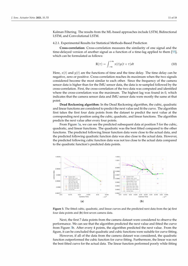
Dead Reckoning algorithm: In the Dead Reckoning algorithm, the cubic, quadraticand linear functions are considered to predict the next value and fit the curve. The algorithmfirst takes the first four data points from the dataset to predict the next value at thecorresponding next position using the cubic, quadratic, and linear functions. The algorithmpredicts the next value after every four points.

From Figure 3a, we can see the predicted subsequent data at position 5 for the cubic,quadratic, and linear functions. The quadratic was the best fitted compared to the otherfunctions. The predicted following linear function data were close to the actual data, andthe predicted following quadratic function data was also close to the actual data. However,the predicted following cubic function data was not too close to the actual data comparedto the quadratic function’s predicted data points.

8.51 8.515 8.52 8.525 8.53 8.535

Camera Time 1010

0.99975

0.9998

0.99985

0.9999

0.99995

1

1.00005

ca

me

ra d

ata

(a)

8.51 8.515 8.52 8.525 8.53 8.535 8.54 8.545 8.55 8.555

Camera Time 1010

0.9992

0.9993

0.9994

0.9995

0.9996

0.9997

0.9998

0.9999

1

1.0001

1.0002

ca

me

ra d

ata

(b)

Figure 3. The fitted cubic, quadratic, and linear curves and the predicted next data from the (a) firstfour data points and (b) first seven camera data.

Next, the first 7 data points from the camera dataset were considered to observe theperformance. We can see that the algorithm predicted the next value and fitted the curvefrom Figure 3b. After every 4 points, the algorithm predicted the next value. From thefigure, it can be concluded that quadratic and cubic functions were suitable for curve fitting.

However, if all of the data from the camera dataset was considered, the quadraticfunction outperformed the cubic function for curve fitting. Furthermore, the linear was notthe best fitted curve for the actual data. The linear function performed poorly while fitting

J. Sens. Actuator Netw. 2021, 10, 53 12 of 18

the curve for the actual data compared to the other two functions. Figure 4 represents thepredicted values of the whole dataset for all the three functions mentioned earlier.

Figure 4. The fitted cubic, quadratic, and linear curves and the predicted next data for all camera data.

Next, the total length for the camera dataset for the cubic, quadratic, and linearfunctions is compared. Figure 5a shows the actual value far away from the predicted valuesby quadratic and cubic functions. From the figure, we can see that the quadratic functionoutperformed the other two functions while predicting the data.

When the previous data with respect to the actual data and the predicted data iscompared, how much the actual data needs to be refined can be analyzed. In this case, itcan be seen that the quadratic property/function was the preferred property/function. Atthe same time, the cubic property also performed close to the quadratic property comparedto the linear function.

8.4 8.6 8.8 9 9.2 9.4 9.6 9.8 10 10.2

Camera Time 1010

0

0.002

0.004

0.006

0.008

0.01

0.012

0.014

0.016

Le

ng

th o

f sa

mp

les f

rom

pre

vio

us p

oin

t

(a)

8.4 8.6 8.8 9 9.2 9.4 9.6 9.8 10 10.2

Camera Time 1010

0

0.001

0.002

0.003

0.004

0.005

0.006

0.007

0.008

0.009

0.01

Pre

dic

ted

Err

or

Difference cubic

Difference quadratic

Difference linear

(b)

Figure 5. (a) Comparison of the total length of the cubic, quadratic, and linear and actual/noprediction length and (b) The differences of the cubic, quadratic, and linear function data from theoriginal data.

The differences of the predicted cubic, quadratic, and linear function data from theoriginal data are plotted in Figure 5b.

Kalman filter: The Kalman filter is applied to the camera dataset to predict the futurevalue. Figure 6a shows that the algorithm predicted the value close to the actual value and

J. Sens. Actuator Netw. 2021, 10, 53 13 of 18

smoothly fitted it. We compare the cubic, quadratic, and linear function methods with theKalman Filtering technique where the Kalman filter quickly predicted the next position,and the predicted value was close to the actual value.

8.52 8.54 8.56 8.58 8.60Time 1e10

0.99975

0.99980

0.99985

0.99990

0.99995

1.00000

Value

Actual dataKalman-Filter predicted data

(a)

0.86 0.88 0.90 0.92 0.94 0.96 0.98 1.001e11

0.84

0.86

0.88

0.90

0.92

0.94

0.96

0.98

1.00

Actual datakalman Filter pred data

(b)

Figure 6. (a) The Kalman filter output for the 30 data points from the data set and (b) the Kalmanfilter output for the all data points from the data set.

In Figure 6b, the prediction was made for the whole dataset, and the curve was fittedcorrectly compared to the cubic, quadratic, and linear function methods. Thus, from theresults above, it can be concluded that the Kalman filter’s prediction was more accurate forthe future position prediction.

4.2.2. Experimental Results for Machine Learning-Based Prediction

To prove the effectiveness of LSTM, Bidirectional LSTM, and Convolutional LSTM, thesame dataset and operating environment were used. The system’s configuration used toconduct the experiments was an Intel i5-4700H 2.6 GHz, 16 GBs of RAM, 500 GB hard disk,and Windows 10 operating system. The dataset was split into 70% and 30% for trainingand testing. The training was executed for 50 epochs. Two hidden dense layers in theLSTM, one dense layer in bidirectional, and one hidden dense layer Convolutional LSTMwere used. The optimizer was Adam, and the loss function of the root mean square error(RMSE) was used to train the model.

Prediction using LSTM, Bidirectional LSTM, and Convolutional LSTM: Figures 7–9illustrates the prediction results for LSTM, Bidirectional LSTM, and Convolutional LSTM.These methods are based on the loss function RMSE.

0.992 0.994 0.996 0.998 1.000 1.002 1.004 1.006Time in seconds 1e11

0.9575

0.9600

0.9625

0.9650

0.9675

0.9700

0.9725

0.9750

0.9775

Camera data value

LSTM based prediction

Actual valuepredicted test Value

(a)

0.86 0.88 0.90 0.92 0.94 0.96 0.98 1.00Time in seconds 1e11

0.84

0.86

0.88

0.90

0.92

0.94

0.96

0.98

1.00

Camera da

ta value

LSTM based prediction

Actua valuePredicted train valuepredicted test Value

(b)

Figure 7. LSTM prediction output for the (a) 30 data points and (b) all data points from the data set.

J. Sens. Actuator Netw. 2021, 10, 53 14 of 18

0.992 0.994 0.996 0.998 1.000 1.002 1.004 1.006Time in seconds 1e11

0.955

0.960

0.965

0.970

0.975

Camera da

ta value

Bi-LSTM based prediction

Actual valuepredicted test Value

(a)

0.86 0.88 0.90 0.92 0.94 0.96 0.98 1.00Time in seconds 1e11

0.84

0.86

0.88

0.90

0.92

0.94

0.96

0.98

1.00

Cam

era

data

val

ue

Bi-LSTM based prediction

Actua valuePredicted train valuepredicted test Value

(b)

Figure 8. Bidirectional LSTM prediction output for the (a) 30 data points and (b) all data points fromthe data set.

0.992 0.994 0.996 0.998 1.000 1.002 1.004 1.006Time in seconds 1e11

0.960

0.965

0.970

0.975

Camera data value

Convolutional LSTM based prediction

Actual valuepredicted test Value

(a)

0.86 0.88 0.90 0.92 0.94 0.96 0.98 1.00Time in seconds 1e11

0.84

0.86

0.88

0.90

0.92

0.94

0.96

0.98

1.00

Camera da

ta value

Convolutional LSTM based prediction

Actua valuePredicted train valuepredicted test Value

(b)

Figure 9. Convolutional LSTM prediction output for the (a) 30 data points and (b) all data pointsfrom the data set.

We found that LSTM, Bidirectional LSTM, and Convolutional LSTM-based predictionoutperformed the Kalman Filtering and Dead Reckoning-based prediction. The details ofthe comparative analysis are provided in Section 4.2.3.

4.2.3. Comparison of Error

Table 1 shows the error comparison of the cubic, quadratic, and linear functionmethods with no prediction data (the difference in the original data from the currentposition to the previous position).

Table 1. Error comparison of cubic, quadratic, and linear function methods with no prediction data.

PredictedFunction Name

MaximumError

MinimumError

AverageError

StandardDeviation Error

Cubic function 0.0096 3.1696× 10−7 0.0016 0.0018Quadraticfunction 0.0051 5.4207× 10−7 9.8735× 10−4 0.0011

Linear function 0.0080 5.8936× 10−7 0.0010 0.0011No prediction 0.0132 5.8524× 10−7 0.0032 0.0032

The no prediction data points were compared to the predicted cubic, quadratic, andlinear data points. Table 1 indicates that the prediction using the quadratic function hada lower error than the no prediction error. However, for the standard deviation (SD), thequadratic and linear function had a similar error. The quadratic function had less errorsthan cubic and linear.

J. Sens. Actuator Netw. 2021, 10, 53 15 of 18

In Table 2, the predicted output of the Kalman filter with our actual data pointsis compared.

Table 2. Error comparison of Kalman filter predicted data and the actual data.

PredictedFunction Name

MaximumError

MinimumError

AverageError

StandardDeviation Error

Kalman filter 0.0193 2.09× 10−6 0.0049 0.0050Actual data 0.9999 0.8436 0.9686 0.0331

Table 2 shows that the actual data points had a higher rate of errors than the Kalmanfilter prediction errors. Thus, the Kalman filter is suitable for prediction, which is illustratedin Figure 5. Additionally, it had more minor errors than the actual value of data points.The predicted data points were close to the actual data points. The results from Table 2indicate that it had significantly fewer errors than the actual data points.

In Table 3, the training and testing RMSE and MAE value from LSTM, BidirectionalLSTM, and Convolutional LSTM model are compared.

Table 3. Error comparison of LSTM, Bidirectional LSTM, and Convolutional LSTM-based predictionRMSE and MAE.

Predicted DeepLearning Model Name

TrainRMSE

TrainMAE

TestRMSE

TestMAE

LSTM 0.02 0.01 0.01 0.001Bidirectional LSTM 0.01 0.01 0.011 0.001

Convolutional LSTM 0.01 0.00 0.012 0.00

The accuracy of the VR sensor prediction presented in Table 3 demonstrates thatthe proposed Convolutional LSTM and Bidirectional LSTM models incurred the smallestRMSE and Convolutional LSTM incurred the smallest MAE in most of the sessions. The ef-fectiveness of the proposed deep-learning-based techniques to predict VR motion positionsis presented by comparing error properties. We found that LSTM performed as superior inevery session of the motion prediction with a small RMSE and MAE. The results depictthat, among the three approaches, CNN-LSTM outperformed the others. The CNN-LSTMhad a MAE of 0.00 and RMSE of 0.00, which were the smallest among the three predictionmodels, and it had high prediction accuracy.

5. Conclusions and Future Work

This paper investigated the latency causing MS in AR and VR systems. We adopteda common prediction algorithm to predict the future values to reduce the system delayresulting in reduced latency. The Dead Reckoning and Kalman Filtering techniques werestudied to predict future data as a common prediction algorithm. We also adopted deep-learning-based methods with three types of LSTM models that could learn general headmotion patterns of VR sensors and predict future viewing directions and locations basedon previous traces.

On a real motion trace dataset with low MAE and RMSE, the system performedwell. The error was compared with no prediction values. We found that the predictedvalues had a minor error when compared with no prediction. While using the DeadReckoning algorithm, the quadratic function had less errors than the cubic and linearfunctions. However, the fitted curve was not right for the quadratic value.

The error property was relatively more minor in the Dead Reckoning algorithm thanwith the Kalman Filtering predicted error results. While deploying the deep-learning-based techniques, the Convolutional LSTM, and Bidirectional LSTM were more effectiveat learning temporal features from the data set. The prediction output can suffer if thenumber of time lags in historical data is insufficient.

J. Sens. Actuator Netw. 2021, 10, 53 16 of 18

However, the model still has certain shortcomings. For instance, we only considereda small amount of data for training and testing since the experiment only had a limitedamount of real-world data from VR sensors. Potential future research would focus onapplying our method with a large, real-world dataset from VR devices.

Since the proposed method showed minimal errors with a high prediction rate, basedon the experimental results, we conclude that our prediction model can reduce significantlysystem latency by predicting future values, which could ultimately help to reduce MS inAR and VR environments.

Author Contributions: Conceptualization, R.K.K. and S.P.; Formal analysis, R.K.K., A.R. and S.P.;Investigation, R.K.K. and S.P.; Methodology, R.K.K. and S.P.; Resources, R.K.K. and S.P.; Supervision,R.K.K., A.R. and S.P.; Writing—original draft, R.K.K. and S.P.; Writing—review & editing, R.K.K.,A.R. and S.P. All authors have read and agreed to the published version of the manuscript.

Funding: This research received no external funding.

Data Availability Statement: The data presented in this study are available on request from thecorresponding author.

Conflicts of Interest: The authors declare no conflict of interest.

References1. Lawson, B.D. Motion Sickness Symptomatology and Origins. 2014. Available online: https://www.taylorfrancis.com/chapters/

mono/10.1201/b17360-33/motion-sickness-symptomatology-origins-kelly-hale-kay-stanney (accessed on 1 September 2020).2. Wood, C.D.; Kennedy, R.E.; Graybiel, A.; Trumbull, R.; Wherry, R.J. Clinical Effectiveness of Anti-Motion-Sickness Drugs:

Computer Review of the Literature. JAMA 1966, 198, 1155–1158. [CrossRef]3. Azad Balabanian, P.L. Motion Sickness in VR: Adverse Health Problems in VR Part I. 2016. Available online: https://researchvr.

podigee.io/5-researchvr-005 (accessed on 5 August 2020).4. Reason, J.T. Motion sickness adaptation: A neural mismatch model. J. R. Soc. Med. 1978, 71, 819–829. [CrossRef] [PubMed]5. Wiker, S.; Kennedy, R.; McCauley, M.; Pepper, R. Susceptibility to seasickness: Influence of hull design and steaming direction.

Aviat. Space Environ. Med. 1979, 50, 1046–1051.6. Paul, S.; Ni, Z.; Ding, F. An Analysis of Post Attack Impacts and Effects of Learning Parameters on Vulnerability Assessment of

Power Grid. In Proceedings of the 2020 IEEE Power Energy Society Innovative Smart Grid Technologies Conference (ISGT),Washington, DC, USA, 17–20 February 2020; pp. 1–5. [CrossRef]

7. Sunny, M.R.; Kabir, M.A.; Naheen, I.T.; Ahad, M.T. Residential Energy Management: A Machine Learning Perspective. InProceedings of the 2020 IEEE Green Technologies Conference(GreenTech), Oklahoma City, OK, USA, 1–3 April 2020; pp. 229–234.[CrossRef]

8. Paul, S.; Ding, F.; Kumar, U.; Liu, W.; Ni, Z. Q-Learning-Based Impact Assessment of Propagating Extreme Weather onDistribution Grids. In Proceedings of the 2020 IEEE Power Energy Society General Meeting (PESGM), Montreal, QC, Canada,3–6 August 2020; pp. 1–5. [CrossRef]

9. Ni, Z.; Paul, S. A Multistage Game in Smart Grid Security: A Reinforcement Learning Solution. IEEE Trans. Neural Netw. Learn.Syst. 2019, 30, 2684–2695. [CrossRef]

10. Paul, S.; Ni, Z.; Mu, C. A Learning-Based Solution for an Adversarial Repeated Game in Cyber–Physical Power Systems. IEEETrans. Neural Netw. Learn. Syst. 2020, 31, 4512–4523. [CrossRef]

11. Alsamhi, S.; Ma, O.; Ansari, S. Convergence of Machine Learning and Robotics Communication in Collaborative Assembly:Mobility, Connectivity and Future Perspectives. J. Intell. Robot. Syst. 2020, 98. [CrossRef]

12. Maity, N.G.; Das, S. Machine learning for improved diagnosis and prognosis in healthcare. In Proceedings of the 2017 IEEEAerospace Conference, Big Sky, MT, USA, 4–11 March 2017; pp. 1–9. [CrossRef]

13. Ahsan, M.M.; Ahad, M.T.; Soma, F.A.; Paul, S.; Chowdhury, A.; Luna, S.A.; Yazdan, M.M.S.; Rahman, A.; Siddique, Z.; Huebner,P. Detecting SARS-CoV-2 From Chest X-Ray Using Artificial Intelligence. IEEE Access 2021, 9, 35501–35513. [CrossRef]

14. Ünal, Z. Smart Farming Becomes Even Smarter With Deep Learning—A Bibliographical Analysis. IEEE Access 2020,8, 105587–105609. [CrossRef]

15. Alahi, A.; Goel, K.; Ramanathan, V.; Robicquet, A.; Fei-Fei, L.; Savarese, S. Social lstm: Human trajectory prediction in crowdedspaces. In Proceedings of the IEEE Conference on Computer Vision and Pattern Recognition,Las Vegas, NV, USA, 27–30 June2016; pp. 961–971.

16. Martinez, J.; Black, M.J.; Romero, J. On human motion prediction using recurrent neural networks. In Proceedings of the IEEEConference on Computer Vision and Pattern Recognition (CVPR), Las Vegas, NV, USA, 27–30 June 2016; pp. 2891–2900.

17. Hou, X.; Dey, S.; Zhang, J.; Budagavi, M. Predictive view generation to enable mobile 360-degree and VR experiences. In Proceed-ings of the 2018 Morning Workshop on Virtual Reality and Augmented Reality Network, Budapest, Hungary, 24 August 2018;pp. 20–26.

J. Sens. Actuator Netw. 2021, 10, 53 17 of 18

18. Fan, C.L.; Lee, J.; Lo, W.C.; Huang, C.Y.; Chen, K.T.; Hsu, C.H. Fixation prediction for 360 video streaming in head-mountedVirtual Reality. In Proceedings of the 27th Workshop on Network and Operating Systems Support for Digital Audio and Video,Taipei, Taiwan, 20–23 June 2017; pp. 67–72.

19. Hou, X.; Lu, Y.; Dey, S. Wireless VR/AR with edge/cloud computing. In Proceedings of the 2017 26th International Conferenceon Computer Communication and Networks (ICCCN),Vancouver, BC, Canada, 31 July–3 August 2017; pp. 1–8.

20. Perfecto, C.; Elbamby, M.S.; Ser, J.D.; Bennis, M. Taming the Latency in Multi-User VR 360°: A QoE-Aware Deep Learning-AidedMulticast Framework. IEEE Trans. Commun. 2020, 68, 2491–2508. [CrossRef]

21. Elbamby, M.S.; Perfecto, C.; Bennis, M.; Doppler, K. Toward low-latency and ultra-reliable Virtual Reality. IEEE Netw. 2018,32, 78–84. [CrossRef]

22. Tiiro, A. Effect of Visual Realism on Cybersickness in Virtual Reality. Univ. Oulu 2018, 350. Available online: http://urn.fi/URN:NBN:fi:oulu-201802091218 (accessed on 5 August 2020).

23. Kennedy, R.S.; Lane, N.E.; Berbaum, K.S.; Lilienthal, M.G. Simulator sickness questionnaire: An enhanced method for quantifyingsimulator sickness. Int. J. Aviat. Psychol. 1993, 3, 203–220. [CrossRef]

24. Sensory Conflict Theory. Available online: https://www.oxfordreference.com/view/10.1093/oi/authority.20110803100454911(accessed on 24 November 2020).

25. Lu, D. Virtual Reality Sickness during Immersion: An Investigation Ofpotential Obstacles towards General Accessibility of VRTechnology. 2016. Available online: https://www.diva-portal.org/smash/get/diva2:1129675/FULLTEXT01.pdf (accessed on 12January 2021).

26. Rouse, M. Field of View (FOV). 2017. Available online: https://whatis.techtarget.com/definition/field-of-view-FOV (accessedon 5 August 2020).

27. Wilson, M.L. The Effect of Varying Latency in a Head-Mounted Display on Task Performance and Motion Sickness. 2016.Available online: https://tigerprints.clemson.edu/cgi/viewcontent.cgi?article=2689&context=all_dissertations (accessed on 20September 2020).

28. Wagner, D. Motion to Photon Latency in Mobile AR and VR. 2018. Available online: https://medium.com/@DAQRI/motion-to-photon-latency-in-mobile-ar-and-vr-99f82c480926 (accessed on 5 August 2020).

29. Hunt, C.L.; Sharma, A.; Osborn, L.E.; Kaliki, R.R.; Thakor, N.V. Predictive trajectory estimation during rehabilitative tasks inaugmented reality using inertial sensors. In Proceedings of the 2018 IEEE Biomedical Circuits and Systems Conference (BioCAS),Cleveland, OH, USA, 17–19 October 2018; pp. 1–4.

30. Zheng, F.; Whitted, T.; Lastra, A.; Lincoln, P.; State, A.; Maimone, A.; Fuchs, H. Minimizing latency for augmented realitydisplays: Frames considered harmful. In Proceedings of the 2014 IEEE International Symposium on Mixed and AugmentedReality (ISMAR), Munich, Germany, 10–12 September 2014; pp. 195–200.

31. Boger, Y. Understanding Predictive Tracking and Why It’s Important for AR/VR Headsets. 2017. Available online: https://www.roadtovr.com/understanding-predictive-tracking-important-arvr-headsets/ (accessed on 7 August 2020).

32. Richter, F.; Zhang, Y.; Zhi, Y.; Orosco, R.K.; Yip, M.C. Augmented Reality Predictive Displays to Help Mitigate the Effectsof Delayed Telesurgery. In Proceedings of the 2019 International Conference on Robotics and Automation (ICRA), MontrealConvention Center, Montreal, QC, Canada, 20–24 May 2019; pp. 444–450.

33. Azuma, R.T. Predictive Tracking for Augmented Reality. Ph.D. Thesis, University of North Carolina, Chapel Hill, NC, USA, 1995.34. Akatsuka, Y.; Bekey, G.A. Compensation for end to end delays in a VR system. In Proceedings of the IEEE 1998 Virtual Reality

Annual International Symposium (Cat. No.98CB36180), Atlanta, GA, USA, 14–18 March 1998; pp. 156–159.35. Butepage, J.; Black, M.J.; Kragic, D.; Kjellstrom, H. Deep representation learning for human motion prediction and classification.

In Proceedings of the IEEE Conference on Computer Vision and Pattern Recognition, Honolulu, HI, USA, 21–26 July 2017;pp. 6158–6166.

36. Greff, K.; Srivastava, R.K.; Koutník, J.; Steunebrink, B.R.; Schmidhuber, J. LSTM: A search space odyssey. IEEE Trans. Neural Netw.Learn. Syst. 2016, 28, 2222–2232. [CrossRef] [PubMed]

37. Liu, J.; Shahroudy, A.; Xu, D.; Wang, G. Spatio-temporal lstm with trust gates for 3d human action recognition. In Proceedings ofthe European Conference on Computer Vision, Amsterdam, The Netherlands, 8–16 October 2016; pp. 816–833.

38. Graves, A.; Mohamed, A.r.; Hinton, G. Speech recognition with deep recurrent neural networks. In Proceedings of the 2013 IEEEInternational Conference on Acoustics, Speech and Signal Processing, Vancouver, BC, Canada, 26–31 May 2013; pp. 6645–6649.

39. Lipton, Z.C.; Berkowitz, J.; Elkan, C. A critical review of recurrent neural networks for sequence learning. arXiv 2015,arXiv:1506.00019.

40. Jain, A.; Zamir, A.R.; Savarese, S.; Saxena, A. Structural-rnn: Deep learning on spatio-temporal graphs. In Proceedings of theIEEE Conference on Computer Vision and Pattern Recognition, Las Vegas, NV, USA, 26 June–1 July 2016; pp. 5308–5317.

41. Zaremba, W.; Sutskever, I.; Vinyals, O. Recurrent neural network regularization. arXiv 2014, arXiv:1409.2329.42. Duan, Y.; Yisheng, L.; Wang, F.Y. Travel time prediction with LSTM neural network. In Proceedings of the 2016 IEEE 19th

international conference on intelligent transportation systems (ITSC), Rio de Janeiro, Brazil, 1–4 November 2016; pp. 1053–1058.43. Cho, K.; Van Merriënboer, B.; Gulcehre, C.; Bahdanau, D.; Bougares, F.; Schwenk, H.; Bengio, Y. Learning phrase representations

using RNN encoder-decoder for statistical machine translation. arXiv 2014, arXiv:1406.1078.44. Schuster, M.; Paliwal, K.K. Bidirectional recurrent neural networks. IEEE Trans. Signal Process. 1997, 45, 2673–2681. [CrossRef]

J. Sens. Actuator Netw. 2021, 10, 53 18 of 18

45. Kim, Y.; Sa, J.; Chung, Y.; Park, D.; Lee, S. Resource-efficient pet dog sound events classification using LSTM-FCN based ontime-series data. Sensors 2018, 18, 4019. [CrossRef]

46. Hashida, S.; Tamura, K. Multi-channel mhlf: Lstm-fcn using macd-histogram with multi-channel input for time series classifica-tion. In Proceedings of the 2019 IEEE 11th International Workshop on Computational Intelligence and Applications (IWCIA),Hiroshima, Japan, 9–10 November 2019; pp. 67–72 .

47. Zhou, Q.; Wu, H. NLP at IEST 2018: BiLSTM-attention and LSTM-attention via soft voting in emotion classification. In Proceedingsof the 9th Workshop on Computational Approaches to Subjectivity, Sentiment and Social Media Analysis, Brusssels, Belgium,31 October–1 November 2018; pp. 189–194.

48. Graves, A.; Schmidhuber, J. Framewise phoneme classification with bidirectional LSTM and other neural network architectures.Neural Netw. 2005, 18, 602–610. [CrossRef]

49. Zhao, Y.; Yang, R.; Chevalier, G.; Shah, R.C.; Romijnders, R. Applying deep bidirectional LSTM and mixture density network forbasketball trajectory prediction. Optik 2018, 158, 266–272. [CrossRef]

50. Chen, T.; Xu, R.; He, Y.; Wang, X. Improving sentiment analysis via sentence type classification using BiLSTM-CRF and CNN.Expert Syst. Appl. 2017, 72, 221–230. [CrossRef]

51. Qin, L.; Yu, N.; Zhao, D. Applying the convolutional neural network deep learning technology to behavioural recognition inintelligent video. Tehnicki Vjesn. 2018, 25, 528–535.

52. Hu, Y. Stock market timing model based on convolutional neural network–a case study of Shanghai composite index. Financ.Econ. 2018, 4, 71–74.

53. Rachinger, C.; Huber, J.B.; Müller, R.R. Comparison of convolutional and block codes for low structural delay. IEEE Trans.Commun. 2015, 63, 4629–4638. [CrossRef]

54. Zhao, Z.; Chen, W.; Wu, X.; Chen, P.C.; Liu, J. LSTM network: A deep learning approach for short-term traffic forecast. IET Intell.Transp. Syst. 2017, 11, 68–75. [CrossRef]

55. Lei Zhang.; Xiaolin Wu. On cross correlation based-discrete time delay estimation. In Proceedings of the Proceedings, (ICASSP’05), IEEE International Conference on Acoustics, Speech, and Signal Processing, Philadelphia, PA, USA, 23–25 March 2005;pp. 981–984.