Instructions for use

Title A Study on Robust Speech Recognition with Time Varying Speech Features

Author(s) Mufungulwa, George

Citation 北海道大学. 博士(情報科学) 甲第12944号

Issue Date 2017-12-25

DOI 10.14943/doctoral.k12944

Doc URL http://hdl.handle.net/2115/68114

Type theses (doctoral)

File Information George_Mufungulwa.pdf

Hokkaido University Collection of Scholarly and Academic Papers : HUSCAP

FO

UNDED

18

76

HOKKA

IDO UNIV

ERSITY

FO

UNDED

18

76

HOKKA

IDO UNIV

ERSITY

Doctoral Thesis

A STUDY ON ROBUST SPEECH RECOGNITION WITHTIME VARYING SPEECH FEATURES

Author:Mr. George Mufungulwa

Superviser:Prof. Yoshikazu MIYANAGA

Examiners:Prof. Kunimasa SAITOH

Prof. Takeo OHGANE Prof. Hiroshi TSUTSUI

A thesis submitted in fulfillment of the requirementsfor the degree of Doctor of Philosophy

in the Division of Information Communication NetworksLaboratory (ICNL)

Graduate School of Information Science and TechnologyHokkaido University

Sapporo, Hokkaido, Japan.

A STUDY ON ROBUST SPEECH RECOGNITION WITH TIME

VARYING SPEECH FEATURES

By

George Mufungulwa

FO

UNDED

18

76

HOKKA

IDO UNIV

ERSITY

FO

UNDED

18

76

HOKKA

IDO UNIV

ERSITY

DOCTORAL THESIS

Supervisor: Prof. Dr. Eng. Yoshikazu Miyanaga

Information Communication Networks Laboratory (ICNL)

Graduate School of Information Science and Technology

Hokkaido University, Japan.

Abstract

Speech feature extraction algorithms have become popular. Speech features can be used

for various applications: biometric recognition, speech recognition, speaker identifica-

tion, and so on. In these applications, a good speech feature can be obtained using

Mel frequency cepstrum Coefficients (MFCC), Linear Predictive Coding (LPC), Time

varying LPC (TVLPC), Perceptual Linear Predictive (PLP) among others. This thesis

focuses on the use of TVLPC among feature extraction algorithms to improve the robust-

ness of automatic speech recognition (ASR) systems against various multiplicative and

additive noises. Time varying speech features (TVSF) are implemented in ASR with

the aim of improving the recognition accuracy on a number of small set of reference

speech databases. The significance of the study is based on the fact that both additive

and multiplicative noises cause great performance degradation of ASR systems, thereby

limiting the speech recognition accuracy in real environments. For this reason, feature

correction, feature compensation and normalization approaches are considered in order

to improve the robustness of a speech recognition system.

The performance degradation is partly due to statistical mismatch between trained

acoustic model of clean speech features and noisy testing speech features. For the pur-

pose of reducing the feature-model mismatch, corrective, compensation as well as nor-

malization techniques are employed both during training and testing of speech features.

In order to achieve improved system performance, normalization in modulation

i

spectrum domain is used to remove non-speech components over a certain frequency

range using running spectrum analysis (RSA) as a band pass filter. In comparison to

other noise reduction techniques used in this study on robust speech recognition, the

RSA filter has an advantage due to its adaptable parameters, that is, the first and second

pass band frequencies can easily be adjusted accordingly. In addition, speech feature

enhancement using dynamic range adjustment (DRA) is utilized. The enhancement is

aimed at correcting the difference between clean and noisy speech features by normal-

izing amplitude of speech features. For the purpose of channel normalization, cepstrum

mean subtraction (CMS) is used in this study.

Two alternative time varying speech features (TVSF) methods are being proposed

and compared with conventional Mel frequency cepstral coefficients (MFCC) features

for noisy speech recognition.

The first experimental study shows that fast Fourier transform (FFT) based Mel fre-

quency cepstrum coefficients (MFCCs) with directly converted time varying linear pre-

diction (TVLPC) based MFCCs, which in this study is defined as time varying speech

features (TVSF), shows a competitive recognition accuracy performance to that of FFT

based MFCCs alone.

In the second experimental study, robustness of speech recognition is further im-

proved by applying mel filtering and logarithmic transformations to short time win-

dowed time varying coefficients before converting to cepstrum coefficients in place of

direct-converted TVLPC speech features. Results show that RSA produces better per-

formance than DRA and CMS/DRA on both similar pronunciation phrases and phrases

uttered by elderly persons. Experimental study shows that the use of time varying speech

features (TVSP) can produce improved speech recognition accuracy even if there is a

mismatch between the training and testing data sets.

ii

Acknowledgments

I thank the Living God Almighty for my life. God is the source of Knowledge, wisdom

and understanding. Without Him, man’s understanding is but ignorance.

I would like to sincerely thank my supervisor, Prof. Yoshikazu Miyanaga, for his

invaluable encouragement, suggestions and support and for providing an excellent re-

search environment. His knowledge, suggestions and discussions greatly contributed in

me understanding research in automatic speech recognition systems and digital signal

processing in general.

I gratefully acknowledge Professor Tsutsui from our laboratory. I will always appre-

ciate his guidance and his support during the time of this research. Through interactions

with him, I have learnt that achieving research of high impact is not just about knowl-

edge acquisition but also skills and paying attention to detail with emphasis on quality.

A very special thanks goes to Professor Alia Asheralieva who was at that time at

our laboratory and is a post doctor at Singapore University of Technology and Design

in Singapore. Her thoughtful critique made me seek a deeper understanding of my area

of research, particularly on publications.

The numerous discussions with all of them and their advice have been an invaluable

contribution to my effort in further developing my understanding of signal processing

algorithms and information theory.

All this would not have happened without the generous support of my sponsors.

iii

Being one of the recipients of the Hokkaido University President’s Fellowship Award

in 2013 and later the Monbukakusho Honors Scholarship for Privately-Financed Inter-

national students from October 2016 to March 2017 has made it possible for me to

complete my studies.

My appreciation also goes to the Thesis defense committee members: Prof. Kuni-

masa Saitoh, Prof. Takeo Ohgane, Prof. Hiroshi Tsutsui and Prof. Yoshikazu Miyanaga

from the graduate school of information science and technology (IST), Hokkaido Uni-

versity.

I am also extremely grateful to the present and past members of the information

communication network laboratory (ICNL). My daily interactions with them saved as

an informal cultural exchange set-up. I thank all those who assisted me in anyway that

I may not directly explain.

I wish to appreciate the following: Dr. Chitondo Lufeyo, my former grade 7 teacher,

Mr Zumba Mwali for looking after me in the time of need, Mr. Ngoma Makosana

(late) for his invaluable advice and mentorship during my undergraduate studies, Mr.

George Nawa, for his support during my search for employment, Mr. Daniel Kasakula

for spiritual guidance during my undergraduate internship. You all have been my role

models through your unique contributions to my humble academic achievement.

From a personal perspective, I would like to express my gratitude to my parents, my

late father, Mr. Giddeon Mufungulwa and my mother, Ms. Easter Chungu. I am very

grateful to you for your sacrifices and for teaching me to be hard working. Last but not

the least, I wish to thank my family for their patience and understanding.

iv

Contents

Abstract i

Acknowledgments iii

List of Tables x

List of Figures xiii

List of Acronyms xiv

1 Introduction 1

1.1 Background . . . . . . . . . . . . . . . . . . . . . . . . . . . . . . . . 1

1.2 Motivation . . . . . . . . . . . . . . . . . . . . . . . . . . . . . . . . . 10

1.3 Thesis overview . . . . . . . . . . . . . . . . . . . . . . . . . . . . . . 14

1.4 Summary of contributions . . . . . . . . . . . . . . . . . . . . . . . . 17

2 Fundamentals of speech recognition 19

2.1 Standard method for speech recognition . . . . . . . . . . . . . . . . . 19

2.2 Speech feature extraction . . . . . . . . . . . . . . . . . . . . . . . . . 20

2.2.1 Conventional FFT-based feature extraction . . . . . . . . . . . 22

2.2.2 TVSF algorithm of direct TVLPC . . . . . . . . . . . . . . . . 30

2.2.3 TVSF algorithm of mel-based TVLPC . . . . . . . . . . . . . . 33

v

2.2.4 Influence of TVLPC coefficient gain . . . . . . . . . . . . . . . 37

2.3 Proposed feature model . . . . . . . . . . . . . . . . . . . . . . . . . . 40

2.3.1 Definition of models . . . . . . . . . . . . . . . . . . . . . . . 40

2.4 Feature classification techniques . . . . . . . . . . . . . . . . . . . . . 41

2.4.1 Artificial neural networks . . . . . . . . . . . . . . . . . . . . 43

2.4.2 Hidden Markov model method . . . . . . . . . . . . . . . . . 44

2.5 Fundamentals of voice activity detection . . . . . . . . . . . . . . . . . 45

2.6 Effects of noise on speech . . . . . . . . . . . . . . . . . . . . . . . . 47

2.6.1 Noise data . . . . . . . . . . . . . . . . . . . . . . . . . . . . . 48

3 Voice Activity Detection 55

3.1 VAD fundamentals . . . . . . . . . . . . . . . . . . . . . . . . . . . . 55

3.2 Short-time energy algorithm . . . . . . . . . . . . . . . . . . . . . . . 57

3.3 Short term autocorrelation algorithm . . . . . . . . . . . . . . . . . . . 60

3.4 Zero-crossing rate algorithm . . . . . . . . . . . . . . . . . . . . . . . 62

4 Noise Reduction 67

4.1 Robust speech technology . . . . . . . . . . . . . . . . . . . . . . . . 67

4.1.1 Subtraction methods . . . . . . . . . . . . . . . . . . . . . . . 67

4.1.2 Dynamic range adjustment (DRA) . . . . . . . . . . . . . . . . 69

4.1.3 High-pass filtering . . . . . . . . . . . . . . . . . . . . . . . . 70

4.1.4 Band-pass Filters . . . . . . . . . . . . . . . . . . . . . . . . . 71

5 Robust speech feature extraction 75

5.1 Speech features based on tvLPC . . . . . . . . . . . . . . . . . . . . . 75

5.1.1 Feature enhancement . . . . . . . . . . . . . . . . . . . . . . . 80

5.1.2 Model formulation . . . . . . . . . . . . . . . . . . . . . . . . 80

vi

5.1.3 Band-pass specifications of RSA . . . . . . . . . . . . . . . . . 81

5.1.4 Simulation parameters and conditions of experiments . . . . . . 84

5.1.5 Simulation results and analysis . . . . . . . . . . . . . . . . . . 88

5.1.6 Discussion . . . . . . . . . . . . . . . . . . . . . . . . . . . . 99

5.1.7 Summary . . . . . . . . . . . . . . . . . . . . . . . . . . . . . 101

5.2 Noise suppression in modulation spectrum . . . . . . . . . . . . . . . . 101

5.2.1 Feature extraction method . . . . . . . . . . . . . . . . . . . . 102

5.2.2 Signal Analysis . . . . . . . . . . . . . . . . . . . . . . . . . . 103

5.2.3 Band-pass specifications of RSA . . . . . . . . . . . . . . . . . 106

5.2.4 Simulation parameters and conditions of experiments . . . . . . 107

5.2.5 Simulation results and analysis . . . . . . . . . . . . . . . . . . 110

5.2.6 Discussion . . . . . . . . . . . . . . . . . . . . . . . . . . . . 113

5.2.7 Summary . . . . . . . . . . . . . . . . . . . . . . . . . . . . . 117

6 Discussion of results 118

6.1 Discussion . . . . . . . . . . . . . . . . . . . . . . . . . . . . . . . . . 118

7 Conclusion and Future Work 122

7.1 Conclusion . . . . . . . . . . . . . . . . . . . . . . . . . . . . . . . . 122

7.2 Future work . . . . . . . . . . . . . . . . . . . . . . . . . . . . . . . . 126

Vita 150

vii

List of Tables

5.1 RSA band specifications. Types (a), (b) and (c) are of infinite impulse

response (IIR) type while Types(d) and (e) are of finite impulse response

(FIR) type . . . . . . . . . . . . . . . . . . . . . . . . . . . . . . . . . 82

5.2 Average recognition accuracy (%) of elderly persons using fixed-cut-off

and gradual-cut-off frequency stop bands of 2nd order RSA pass band

on clean speech and on 15 types of noise (from NOISEX-92 database)

using conventional approach at 0 dB, 5 dB, 10 dB and 20 dB SNR . . 83

5.3 Comparative performance in average recognition accuracy (%) of RSA

type(c) and type (e) specifications under 15 types of noise at 10 dB and

20 dB SNR . . . . . . . . . . . . . . . . . . . . . . . . . . . . . . . . 83

5.4 Parameters for 3 Similar Pronunciation phrases and 142 Japanese com-

mon speech phrases . . . . . . . . . . . . . . . . . . . . . . . . . . . . 86

5.5 Parameters for 13 phrases uttered by elderly male persons . . . . . . . . 87

5.6 Average recognition accuracy (%) for similar pronunciation phrases /genki/,

/denki/ and /tenki/ on 15 types of noise at 10 dB and 20 dB SNR . . . . 91

5.7 Average recognition accuracy (%) for similar pronunciation phrases /kyu/,

/juu/ and /chuu/ on 15 types of noise at 10 dB and 20 dB SNR . . . . . 92

5.8 Average recognition accuracy (%) of 13 phrases for elderly male persons

on 15 types of noise at 10 dB and 20 dB SNR . . . . . . . . . . . . . . 92

viii

5.9 Average recognition accuracy (%) for 142 Japanese common speech

phrases on 15 types of noise at 10 dB and 20 dB SNR . . . . . . . . . 92

5.10 Recognition accuracy (%) for 142 Japanese common speech phrases on

clean speech . . . . . . . . . . . . . . . . . . . . . . . . . . . . . . . . 93

5.11 Recognition performance accuracy (%) of the 15 types of noises on 142

Japanese common speech phrases using conventional approach (model

0) at 10 dB and 20 dB SNR of CMS/DRA and RSA . . . . . . . . . . 94

5.12 Average performance indicators (%) for similar pronunciation phrases

/genki/, /denki/ and /tenki/ on 15 types of noise at 10 dB and 20 dB SNR 96

5.13 Average performance indicators (%) of 13 phrases for elderly male peo-

ple on 15 types of noise at 10 dB and 20 dB SNR . . . . . . . . . . . . 96

5.14 Average performance indicators (%) for similar pronunciation phrases

/kyu/, /juu/ and /chuu/ on 15 types of noise at 10 dB and 20 dB SNR . . 97

5.15 Average performance indicators (%) for 142 Japanese common speech

phrases on 15 types of noise at 10 dB and 20 dB SNR . . . . . . . . . 98

5.16 RSA band specifications. Type (a) is wide bandwidth, Types (b), (c), (d)

and (e) are of narrow bandwidths (FIR) type . . . . . . . . . . . . . . . 107

5.17 RSA sub band specifications for wide band-pass. Type (c1) and (c2)

are sub band-pass for Type (c). Type (d1) and Type (d2) are sub band

specifications for Type (d) wide band-pass . . . . . . . . . . . . . . . . 108

5.18 The condition of speech recognition experiments . . . . . . . . . . . . 109

5.19 Average recognition accuracy (%) for 100 words Japanese common speech

phrases on 15 types of noise at 5 dB, 10 dB, 15 dB ,20 dB , and 25 dB

SNR . . . . . . . . . . . . . . . . . . . . . . . . . . . . . . . . . . . . 112

ix

5.20 Average recognition accuracy (%) for 100 words Japanese common speech

phrases on 15 types of noise at 5 dB, 10 dB, 15 dB ,20 dB , and 25 dB

SNR . . . . . . . . . . . . . . . . . . . . . . . . . . . . . . . . . . . . 113

5.21 Summary recognition accuracy(%) of Japanese common speech phrases

on 15 types of noises at 5 dB , 10 dB, 15 dB , 20 dB and 25 dB SNR . 114

5.22 Relative improvement(%) of Japanese common speech phrases on 15

types of noises at 5 dB , 10 dB, 15 dB , 20 dB and 25 dB SNR of RSA

compared with RSF . . . . . . . . . . . . . . . . . . . . . . . . . . . . 115

x

List of Figures

1.1 Block diagram for statistical based ASR system . . . . . . . . . . . . . 6

1.2 MFCC: Complete pipeline for feature extraction . . . . . . . . . . . . . 11

1.3 Steps of identification and recognition of a isolated word . . . . . . . . 12

2.1 ASR system diagram . . . . . . . . . . . . . . . . . . . . . . . . . . . 20

2.2 Block diagram of MFCC feature extraction process . . . . . . . . . . . 22

2.3 Attenuation of Hamming, Hanning, triangle and rectangle window types 25

2.4 Attenuation of rectangular and Hamming windows . . . . . . . . . . . 26

2.5 Feature estimation process with direct converted TVLPC coefficients. . 30

2.6 Feature estimation process using mel Filtered TVLCP Coefficients. . . . 34

2.7 Waveform for 7 frames of a Japanese phrase /genki/ after VAD and

pre-emphasis and magnitude spectrum of normalized tvLPC coefficients

frame-by-frame. . . . . . . . . . . . . . . . . . . . . . . . . . . . . . . 38

2.8 Waveform for 7 frames of a Japanese phrase /denki/ after VAD and

pre-emphasis and magnitude spectrum of normalized tvLPC coefficients

frame-by-frame. . . . . . . . . . . . . . . . . . . . . . . . . . . . . . . 39

2.9 Waveform for 7 frames of a Japanese phrase /tenki/ after VAD and pre-

emphasis and magnitude spectrum of normalized tvLPC coefficients

frame-by-frame. . . . . . . . . . . . . . . . . . . . . . . . . . . . . . . 39

xi

2.10 Proposed concatenated speech features, with model 0 as conventional

approach. . . . . . . . . . . . . . . . . . . . . . . . . . . . . . . . . . 41

2.11 model definitions . . . . . . . . . . . . . . . . . . . . . . . . . . . . . 42

2.12 Short Term energy contour of a Japanese speech phrase /genki/ . . . . . 46

2.13 The effects of increased babble noise on Japanese speech segment /genki/ 51

2.14 (a) The waveform, spectrum and cepstrum of clean speech /genki/ (b)

Spectrum and Cepstrum with babble noise at 20 dB, (c) Spectrum and

Cepstrum with babble noise at 10 dB (d) Spectrum and Cepstrum with

babble noise at 0 dB SNR . . . . . . . . . . . . . . . . . . . . . . . . . 52

2.15 (a) The power spectrum of clean speech /tenki/ (b) power spectrum with

white noise at 10 dB SNR . . . . . . . . . . . . . . . . . . . . . . . . . 53

3.1 Waveform and Autocorrelation of 30 ms Voiced portion of speech /genki/ 61

3.2 Waveform and Autocorrelation of 30 ms Unvoiced portion of speech

/genki/ . . . . . . . . . . . . . . . . . . . . . . . . . . . . . . . . . . . 61

3.3 Waveform of word of clean speech /genki/ . . . . . . . . . . . . . . . . 63

3.4 Short-time energy of frames of clean speech phrase /genki/ . . . . . . . 64

3.5 Zero-crossing rate of frames of clean speech phrase /genki/ . . . . . . . 64

3.6 Noisy speech signal at 10 dB . . . . . . . . . . . . . . . . . . . . . . . 65

3.7 Short-time energy of frames of a noisy speech signal at 10 dB SNR . . . 65

3.8 Zero-crossing rate of frames of a noisy speech signal at 10 dB SNR . . 66

5.1 Waveform for 7 frames of a Japanese phrase /genki/ after VAD and pre-

emphasis and magnitude spectrum of normalized TVLPC coefficients

frame-by-frame. . . . . . . . . . . . . . . . . . . . . . . . . . . . . . . 90

xii

5.2 Waveform for 7 frames of a Japanese phrase /denki/ after VAD and pre-

emphasis and magnitude spectrum of normalized TVLPC coefficients

frame-by-frame. . . . . . . . . . . . . . . . . . . . . . . . . . . . . . . 90

5.3 Waveform for 7 frames of a Japanese phrase /tenki/ after VAD and pre-

emphasis and magnitude spectrum of normalized TVLPC coefficients

frame-by-frame. . . . . . . . . . . . . . . . . . . . . . . . . . . . . . . 91

5.4 MFCC: Complete pipeline for feature extraction . . . . . . . . . . . . . 104

5.5 Implementation of band-pass RSA FIR filter banks for noise suppression 108

5.6 Relative performance improvement(%) on common speech phrases us-

ing 9 sets of RSA filter banks on 15 types of noises. . . . . . . . . . . . 112

xiii

List of Acronyms

ASR Automatic Speech Recognition

CMS Cepstrum Mean Subtraction

DCT Discrete Cosine Transformation

DFT Discrete Fourier Transform

DRA Dynamic Range Adjustment

DTW Dynamic Time Warping

DTX Discontinuous Transmission

FFT Fast Fourier Transform

FIR Finite Impulse Response

HMM Hidden Markov Model

IFFT Inverse Fast Fourier Transform

IIR Infinite Impulse Response

LPC Linear Predictive Coefficients

MFCC Mel-Freqency Cepstrum Coefficients

PLP Perceptual Linear Prediction

RSA Running Spectrum Analysis

RASTA-PLP Relative Spectral Transform

SNR Signal-to-Noise Ratio

SS Spectral Subtraction

xiv

STFT Short Time Fourier Transform

STP Short Term Processing

TVLPC Time Varying Linear Prediction Coefficients

TVSF Time Varying Speech Features

VAD Voice Activity Detection

VC Voice Command

VQ Vector Quantization

ZCR Zero-Crossing Rate

xv

Chapter 1

Introduction

1.1 Background

Speech is one of the most effective modes of interaction between humans or between hu-

man and a machine. In addition, it is the most natural and convenient method of interac-

tion. A speech signal constitutes infinite information. Digital processing of speech sig-

nal is very important for real time and precise automatic voice recognition technology.

Proliferation of such information devices as personal computers, smart-phones, tablet

devices, etc., has enabled voice command (VC) to be a desirable feature in human-to-

machine interaction. Voice-controlled applications have many practical uses including

communication, business location, daily life navigation, among others. In recent times

speech processing has found its applications in health care, telephony, military and peo-

ple with disabilities, among other fields. Today these speech signals are also used in

biometric recognition technologies and communicating with machines.

Although the speech communication technology between human and computer is

experiencing a revolutionary progress in the information industry, speech recognition is

a challenging and interesting problem in and of itself. It is one of the most integrating ar-

1

eas of machine intelligence, since humans do a daily activity of speech recognition. For

this reason, the digital signal processing such as feature extraction and feature match-

ing are the latest study issues of voice signal. In order to extract valuable information

from the speech signal, speech data needs to be pre-processed and analysed. The basic

method used for extracting the features of the voice signal is to find the mel frequency

cepstral coefficients. In order to extract such features, the key stages and their main

purpose areconsidered:

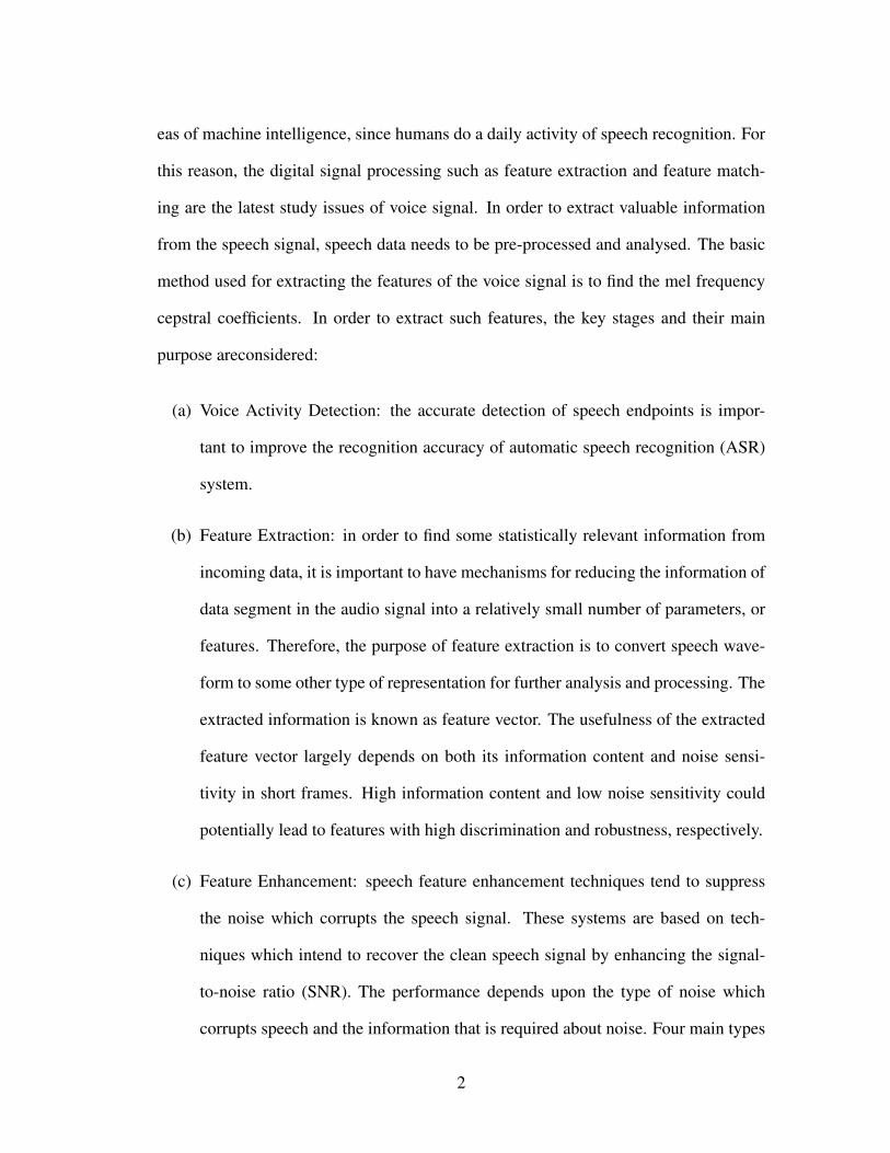
(a) Voice Activity Detection: the accurate detection of speech endpoints is impor-

tant to improve the recognition accuracy of automatic speech recognition (ASR)

system.

(b) Feature Extraction: in order to find some statistically relevant information from

incoming data, it is important to have mechanisms for reducing the information of

data segment in the audio signal into a relatively small number of parameters, or

features. Therefore, the purpose of feature extraction is to convert speech wave-

form to some other type of representation for further analysis and processing. The

extracted information is known as feature vector. The usefulness of the extracted

feature vector largely depends on both its information content and noise sensi-

tivity in short frames. High information content and low noise sensitivity could

potentially lead to features with high discrimination and robustness, respectively.

(c) Feature Enhancement: speech feature enhancement techniques tend to suppress

the noise which corrupts the speech signal. These systems are based on tech-

niques which intend to recover the clean speech signal by enhancing the signal-

to-noise ratio (SNR). The performance depends upon the type of noise which

corrupts speech and the information that is required about noise. Four main types

2

of methods are used for speech enhancement:

(i) Noise Subtraction: this method assumes that noise and speech are uncorre-

lated and additive. In the spectral subtraction approach, the power spectrum

of clean speech is obtained by subtracting the noise power spectrum from the

spectrum of noisy speech. The method assumes that the noise varies so that

the noise estimation obtained during an approximately stationary instance

can be used for suppression.

(ii) Filtering: traditional adaptive filtering techniques have been used for speech

enhancement, but more for speech transmission than for recognition pur-

poses. Unless the noise is stationary and perfectly known, adaptive filtering

technique must usually be done iteratively.

(iii) Use of Markov Models: hidden Markov models (HMM) decomposition is a

method which makes it possible to separate speech from additive noise. The

recognition of a noisy utterance can therefore be carried out by extending the

classical Viterbi decoding algorithm to a search in the state space defined by

the two models. This method is rather computationally demanding.

(iv) Speech Mapping: speech enhancement can be viewed as the process of trans-

forming noisy speech into clean speech by some kind of mapping. For in-

stance, spectral mapping has been implemented by a set of rules obtained by

vector quantization techniques. It is also possible to implement arbitrarily

complex space transformations via connectionist neural networks. Simple

models such as multi-layer perceptions have been trained on learning sam-

ples to realize a mapping of noisy signals to noise-free speech which has

been tested with success in an auditory preference test with human listeners.

3

In this thesis, noise subtraction and filtering is applied.

(d) Modeling Techniques: The objective of modeling technique is to generate speaker

models using speaker specific feature vector. The speaker modeling technique is

classified into two: speaker recognition and speaker identification. The speaker

identification technique automatically identifies who is speaking on basis of in-

dividual information integrated in speech signal. The speaker recognition is also

divided into two parts; that is speaker dependant and speaker independent. In the

speaker independent mode of the speech recognition the computer should ignore

the speaker specific characteristics of the speech signal and extract the intended

message. On the other hand, in case of speaker recognition, the machine should

extract speaker characteristics in the acoustic signal [1].

The following are some of the modeling which can be used in speech recognition

process depending on application [2]; the acoustic-phonetic approach, pattern

recognition approach, template based approach, dynamic time warping, knowl-

edge based approach, statistical based approach, learning based approach, the ar-

tificial intelligence approach and stochastic approach.

Some of these approaches are highlited as follows:

(i) Acoustic-phonetic approach: this approach is based on the theory of acoustic pho-

netics and postulates [3–5]. The earliest approaches to speech recognition were

based on finding speech sounds and providing appropriate labels to these sounds.

This is the basis of the acoustic phonetic approach [6]. Which assumes that there

exist finite, distinctive phonetic units (phonemes) in a spoken language and that

these units are broadly characterized by a set of acoustics properties that are man-

ifested in the speech signal over time.

4

(ii) Pattern recognition approach: the pattern-matching approach [7] [8] [9] involves

two essential steps namely; pattern training and pattern comparison. The essential

feature of this approach is that it uses a well formulated mathematical framework

and establishes consistent speech pattern representations, for reliable pattern com-

parison, from a set of labelled training samples via a formal training algorithm.

A pattern recognition that has been developed over the last two decades has re-

ceived much attention and been applied widely to many practical pattern recog-

nition problems [10]. A speech pattern representation can be in the form of a

speech template or a statistical model (e.g., a Hidden Markov model or HMM)

and can be applied to a sound (smaller than a word), a word, or a phrase. In the

pattern-comparison stage of the approach, a direct comparison is made between

the unknown speeches (the speech to be recognized) with each possible pattern

learned in the training stage in order to determine the identity of the unknown ac-

cording to the goodness of match of the patterns. The pattern-matching approach

has become the predominant method for speech recognition in the last six decades

[11]. Speech recognition is a special case of pattern recognition. Figure 1.1 be-

low shows the processing stages involved in a typical speech recognition system

using this model. There are two phases in supervised pattern recognition, such

are training and testing. The process of extraction of features relevant for classi-

fication is common to both phases. During the training phase, the parameters of

the classification model are estimated using a large number of class ideal models

(training data). During the testing or recognition phase, the features of a test pat-

tern (test speech data) are matched with the trained model of each and every class.

The test pattern is declared to belong to that class whose model matches the test

pattern best.

5

Figure 1.1: Block diagram for statistical based ASR system

(iii) Template based approaches: In template based approaches matching [12] un-

known speech is compared against a set of pre-recorded words (templates) in or-

der to find the best Match. This has the advantage of using perfectly accurate

word models. Template based approach [13] to speech recognition have provided

a family of techniques that have advanced the field considerably during the last

six decades. The underlying idea is that a collection of prototypical speech pat-

terns are stored as reference patterns representing the dictionary of candidates’

words. Recognition is then carried out by matching an unknown spoken utter-

ance with each of these reference templates and selecting the category of the best

matching pattern. Usually templates for entire words are constructed. This has the

advantage that, errors due to segmentation or classification of smaller acoustically

more variable units such as phonemes can be avoided. In turn, each word must

have its own full reference template; template preparation and matching become

prohibitively expensive or impractical as vocabulary size increases beyond a few

6

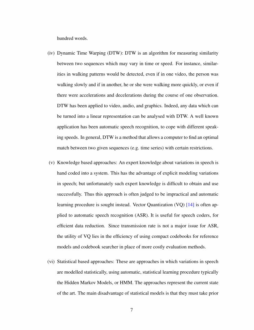
hundred words.

(iv) Dynamic Time Warping (DTW): DTW is an algorithm for measuring similarity

between two sequences which may vary in time or speed. For instance, similar-

ities in walking patterns would be detected, even if in one video, the person was

walking slowly and if in another, he or she were walking more quickly, or even if

there were accelerations and decelerations during the course of one observation.

DTW has been applied to video, audio, and graphics. Indeed, any data which can

be turned into a linear representation can be analysed with DTW. A well known

application has been automatic speech recognition, to cope with different speak-

ing speeds. In general, DTW is a method that allows a computer to find an optimal

match between two given sequences (e.g. time series) with certain restrictions.

(v) Knowledge based approaches: An expert knowledge about variations in speech is

hand coded into a system. This has the advantage of explicit modeling variations

in speech; but unfortunately such expert knowledge is difficult to obtain and use

successfully. Thus this approach is often judged to be impractical and automatic

learning procedure is sought instead. Vector Quantization (VQ) [14] is often ap-

plied to automatic speech recognition (ASR). It is useful for speech coders, for

efficient data reduction. Since transmission rate is not a major issue for ASR,

the utility of VQ lies in the efficiency of using compact codebooks for reference

models and codebook searcher in place of more costly evaluation methods.

(vi) Statistical based approaches: These are approaches in which variations in speech

are modelled statistically, using automatic, statistical learning procedure typically

the Hidden Markov Models, or HMM. The approaches represent the current state

of the art. The main disadvantage of statistical models is that they must take prior

7

modeling assumptions which are answerable to be inaccurate, handicapping the

system performance. In recent years, a new approach to the challenging problem

of conversational speech recognition has emerged, holding a promise to overcome

some fundamental limitations of the conventional Hidden Markov Model (HMM)

approach [15, 16]. This new approach is a radical departure from the current

HMM-based statistical modeling approaches.

(vii) The artificial intelligence approach: the artificial intelligence approach attempts

to mechanize the recognition procedure according to the way a person applies

his intelligence in visualizing, analyzing, and finally making a decision on the

measured acoustic features. Expert system is used widely in this approach [17].

The HMM is a popular statistical tool for modelling a wide range of time series data.

In Speech recognition, HMM has been applied with great success to such problems as

speech classification [18]. Therefore, in this study its application is opted for.

The problem of automatic speech recognition in an adverse environment has at-

tracted many researchers’ attention. The main reason is that the performance of existing

speech recognition systems, designed on assumption of low noise or low interference,

often degrades rapidly in the presence of noise, distortions and articulative effects [19].

Additive noise contaminates the speech signal and changes the data vectors represent-

ing speech. For instance, white noise will tend to reduce the dynamic range, or variance

of cepstral coefficients within the frame. Similarly, speaking in a noisy environment,

where auditory feedback is obstructed by the noise, causes statistically significant ar-

ticulation variability as the speaker attempts to increase the communication efficiency

over the noisy medium. This phenomenon is known as the Lombard effect [20, 21].

These phenomena may produce serious mismatches between the training and recogni-

tion conditions that result in degradation in accuracy. Consequently, most efforts in the

8

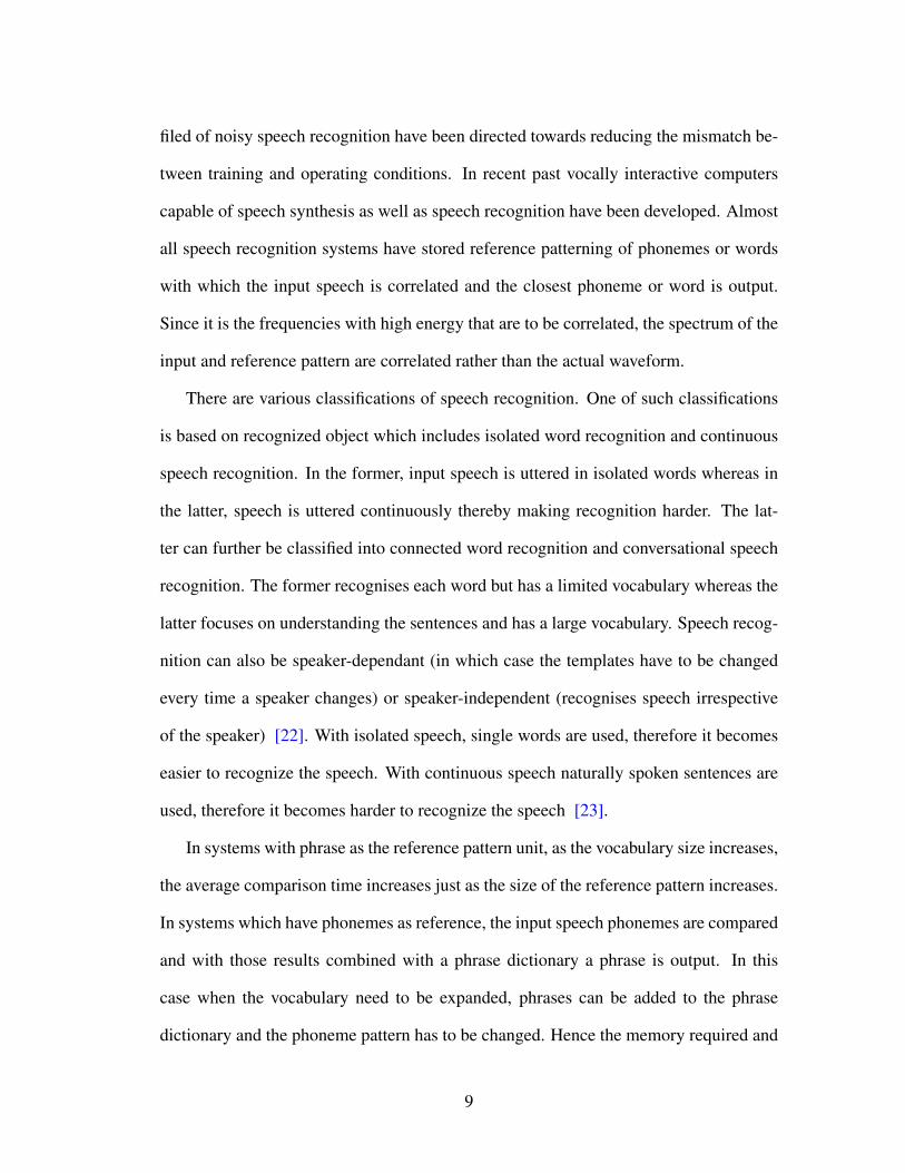
filed of noisy speech recognition have been directed towards reducing the mismatch be-

tween training and operating conditions. In recent past vocally interactive computers

capable of speech synthesis as well as speech recognition have been developed. Almost

all speech recognition systems have stored reference patterning of phonemes or words

with which the input speech is correlated and the closest phoneme or word is output.

Since it is the frequencies with high energy that are to be correlated, the spectrum of the

input and reference pattern are correlated rather than the actual waveform.

There are various classifications of speech recognition. One of such classifications

is based on recognized object which includes isolated word recognition and continuous

speech recognition. In the former, input speech is uttered in isolated words whereas in

the latter, speech is uttered continuously thereby making recognition harder. The lat-

ter can further be classified into connected word recognition and conversational speech

recognition. The former recognises each word but has a limited vocabulary whereas the

latter focuses on understanding the sentences and has a large vocabulary. Speech recog-

nition can also be speaker-dependant (in which case the templates have to be changed

every time a speaker changes) or speaker-independent (recognises speech irrespective

of the speaker) [22]. With isolated speech, single words are used, therefore it becomes

easier to recognize the speech. With continuous speech naturally spoken sentences are

used, therefore it becomes harder to recognize the speech [23].

In systems with phrase as the reference pattern unit, as the vocabulary size increases,

the average comparison time increases just as the size of the reference pattern increases.

In systems which have phonemes as reference, the input speech phonemes are compared

and with those results combined with a phrase dictionary a phrase is output. In this

case when the vocabulary need to be expanded, phrases can be added to the phrase

dictionary and the phoneme pattern has to be changed. Hence the memory required and

9

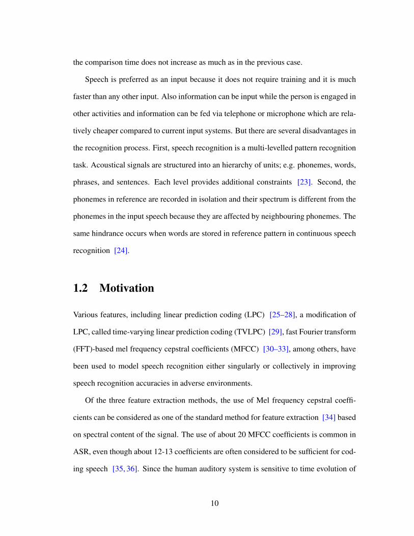
the comparison time does not increase as much as in the previous case.

Speech is preferred as an input because it does not require training and it is much

faster than any other input. Also information can be input while the person is engaged in

other activities and information can be fed via telephone or microphone which are rela-

tively cheaper compared to current input systems. But there are several disadvantages in

the recognition process. First, speech recognition is a multi-levelled pattern recognition

task. Acoustical signals are structured into an hierarchy of units; e.g. phonemes, words,

phrases, and sentences. Each level provides additional constraints [23]. Second, the

phonemes in reference are recorded in isolation and their spectrum is different from the

phonemes in the input speech because they are affected by neighbouring phonemes. The

same hindrance occurs when words are stored in reference pattern in continuous speech

recognition [24].

1.2 Motivation

Various features, including linear prediction coding (LPC) [25–28], a modification of

LPC, called time-varying linear prediction coding (TVLPC) [29], fast Fourier transform

(FFT)-based mel frequency cepstral coefficients (MFCC) [30–33], among others, have

been used to model speech recognition either singularly or collectively in improving

speech recognition accuracies in adverse environments.

Of the three feature extraction methods, the use of Mel frequency cepstral coeffi-

cients can be considered as one of the standard method for feature extraction [34] based

on spectral content of the signal. The use of about 20 MFCC coefficients is common in

ASR, even though about 12-13 coefficients are often considered to be sufficient for cod-

ing speech [35, 36]. Since the human auditory system is sensitive to time evolution of

10

the spectral content of speech signal, an attempt is often made to include the extraction

of this information ,that is, the delta and acceleration as part of feature analysis. These

dynamic coefficients are then concatenated with the static coefficients to make the final

output of feature analysis representation. Figure 1.2 shows the complete MFCC pipeline

Figure 1.2: MFCC: Complete pipeline for feature extraction

For LPC of speech, the speech waveform is modelled as the output of an all-pole

filter. The waveform is partitioned into several short intervals (10-30 ms) during which

the speech signal is assumed to be stationary. For each interval the constant coefficients

of the all-pole filter are estimated by linear prediction by minimizing a squared predic-

tion error criterion. In this thesis, however, a modification of LPC, called time-varying

LPC, which can be used to analyze nonstationary speech signals is considered. In this

method, each coefficient of the all-pole filter is allowed to be time-varying by assuming

it is a linear combination of a set of known time functions.

In comparison, FFT based MFCC is a simple and popular feature extraction method

commonly used in automatic speech recognition (ASR). However, the most notable

11

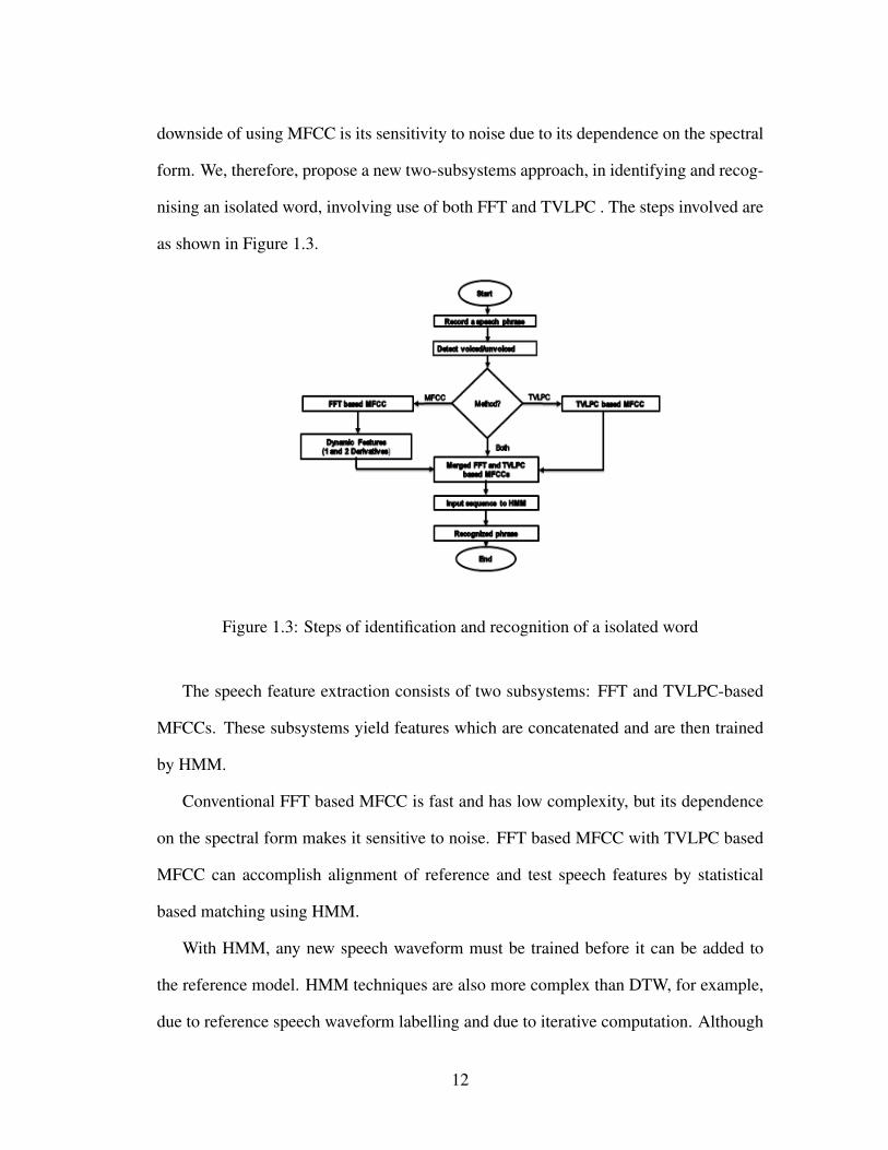
downside of using MFCC is its sensitivity to noise due to its dependence on the spectral

form. We, therefore, propose a new two-subsystems approach, in identifying and recog-

nising an isolated word, involving use of both FFT and TVLPC . The steps involved are

as shown in Figure 1.3.

Figure 1.3: Steps of identification and recognition of a isolated word

The speech feature extraction consists of two subsystems: FFT and TVLPC-based

MFCCs. These subsystems yield features which are concatenated and are then trained

by HMM.

Conventional FFT based MFCC is fast and has low complexity, but its dependence

on the spectral form makes it sensitive to noise. FFT based MFCC with TVLPC based

MFCC can accomplish alignment of reference and test speech features by statistical

based matching using HMM.

With HMM, any new speech waveform must be trained before it can be added to

the reference model. HMM techniques are also more complex than DTW, for example,

due to reference speech waveform labelling and due to iterative computation. Although

12

HMM-based approaches require training [37], for noisy environments, HMM tech-

niques achieve higher accuracy.

In ASR systems, the HMM method has been widely used. The ASR based HMM

consists of two different stages, i.e., training and recognition. For the training stage, a lot

of real speech data should be prepared. After the training stage has been completed, the

system has easily shown high recognition accuracy under low noise circumstances. Re-

cently, since there are several noise reduction methods and speech enhancement meth-

ods against any noises, almost all of ASRs using HMM and noise reduction can show

higher accuracy of speech recognition rate than that given by a conventional standard

HMM based ASR.

In this study, HMMs which are trained by a set of words and phrases are used. Since

the ASR using word based HMM is trained with any detail and important information

of words, e.g., co-articulation, the performance of this ASR can show high accuracy

even in any noisy environments. The challenge, however, is that the training costs of the

word based HMM are normally large. This means, in an event that one word is added to

HMM speech model database, many persons who utter target keywords several times,

are often required. In which case, a prior processing is needed after a large set of speech

database is prepared.

In this thesis, an ASR system is developed that uses time varying speech features

(TVSF). In the proposed method a combination of the FFT-based MFCC with the TVLPC-

based MFCC in a two subsystems feature extraction process using HMM both for train-

ing and recognition is consindered. The combined inter-frame variations (from FFT-

based MFCC) and intra-frame variations (from TVLPC-based MFCC) is envisaged to

improve recognition accuracy. The enhanced technology utilizes information in both

spectral and periodicity of speech signals to overcome the problem of sensitivity to

13

noise.

First, the voice activity detection (VAD) is improved using the short time energy

and zero-crossing rate algorithms. The new proposed approach substantially decreases

the effect of additive noises. The endpoint detection accuracy is also improved. Then,

the use of running spectrum analysis (RSA), cepstrum mean subtraction (CMS), and dy-

namic range adjustment (DRA) on the FFT-based MFCC and DRA only on the TVLPC-

based MFCC to reduce noise are proposed. The two types of TVLPC-based MFCC in-

volve the use of; a) direct converted TVLPC coefficients and b) a mel filter banks and

log transformation TVLCP coefficients. The recognition accuracy with mel filter banks

and log transformed TVLCP cepstrum is better than that of the direct converted TVLPC

cepstrum. In the final analysis, the mel filtered TVLPC-based MFCC is proposed with

HMM be used as a recognizer. The performance of proposed FFT-based MFCC with

mel filter banks TVLPC-based MFCC speech feature extraction approach is similar to

that of FFT-based MFCC only, however, the recognition accuracy is improved notably

under low signal-to-noise ratio (SNR).

1.3 Thesis overview

Chapter 1 describes the background of digital processing of speech, study motivation,

thesis overview and study contributions.

Chapter 2 introduces the standard method for speech recognition, and the steps in-

volved in conventional FFT-based MFCC. Time varying speech feature (TVSF) algo-

rithm of direct TVLPC and TVSF algorithm of mel based TVLPC are discussed. Def-

inition of proposed feature model, feature classification techniques, fundamentals of

voice activity detection, and effects of noise speech are equally introduced.

14

Chapter 3 discusses the voice activity detection (VAD) method with short term en-

ergy, short term autocorrelation and zero-crossing rate (ZCR). The use of a short time

energy is proposed. The proposed approach helps to minimize the effect of pulse-noise.

The endpoint detection accuracy is increased.

Chapter 4 discusses the influence of additive and multiplicative noises. Modula-

tion spectra and noise circustances, the running spectrum filter and running spectrum

analysis algorithm are discussed. In addition, the limitation of band-pass filtering are

highlighted. When speech signal is Fourier transformed, the additive noise can be re-

moved in the frequency component. It is impossible to have the multiplicative noises

successfully removed using Fourier transform only. A Fourier transform of a convolved

signal makes it a multiplicative signal which should be logarithmically transformed to

realize an additive result. The system noise has no time variation factor quite much

compared with speech waveform. Therefore, the modulation spectrum of speech usu-

ally concentrates its energy into around 0 Hz. Accordingly, the important part for speech

recognition can be discriminated from others on the modulation spectrum. In compen-

sating for distortions, CMS is used as normalization method and DRA to minimize the

variability of noise feature values. In DRA, each coefficient of a speech feature is ad-

justed proportionally to its maximum amplitude.

RSA, CMS as normalization method and DRA algorithms are introduced to mini-

mize the variability of noise feature values. In DRA, each coefficient of a speech feature

is adjusted proportionally to its maximum amplitude. Use of CMS/DRA is proposed,

and RSA for noise reduction. The CMS/DRA method improves the accuracy of HMM

efficiently. Band-pass filtering using RSA is used to remove additive noise components

on running spectrum domain. Careful consideration is necessary in designing such a

filter. Excessive elimination of lower modulation frequency band may cause negative

15

values in power spectrum and negative values lead to a problem when power spectrum

is converted to logarithmic power spectrum for obtaining cepstrum.

Chapter 5 evaluates the performance of the proposed time varying speech features

with HMM. Experiments are conducted for the two sets of 3 similar pronounciation

phrases, 13 phrases uttered by elderly people and the 142 common Japanese phrases.

The accuracy of our approach increases with the number of reference speech waveforms

(utterances) available for the reference words. It has been observed that performance of

the proposed approach seems to be influenced by two main factors; first by the type of

noise and second, by the noise reduction technique being applied. It is also observe that

the recognition performance varies depending on the noise levels. It is also noted that

models 1 and 3 perform competitively if not slightly better than model 0. This is an

indication that 1 and 3 dimensional feature components of TVLPC may be adequate to

realize better or slightly better results with our proposed method. By using few compo-

nents the computation time on the part of TVLPC is reduced.

Chapter 6 compares the proposed time varying speech features to those of the con-

ventional approach. There is a difference in tendency between similar pronunciation

phrases and phrases uttered by elderly people. Even though care was taken in designing

the RSA band-pass filter there may be unnecessary components, hence its poor perfor-

mance compared with CMS/DRA. It can cautiously be inferred that the under perfor-

mance exhibited by our proposed method in some cases could be attributed to disconti-

nuities of acoustic units around concatenation points.

Chapter 7 summaries the above research and gives a conclusion to highlight the

research significance. Finally, some possible work for future research are briefly de-

scribed. It is found that concatenating FFT-based MFCC with the TVLPC-based MFCC

to create time varying speech features (TVSF) can improve the speech recognition ca-

16

pability for some models with HMM implementations. The proposed method may be a

simpler solution for speech recognition applications that requires further improvements.

1.4 Summary of contributions

This thesis makes the following contributions:

• By considering the influence of time-varying coefficient gain, frame-by-frame,

we confirm the presence of intra-frame variation in each frame. We aim to eval-

uate the contribution of such variation when appended to features estimated from

inter-frame variation. The resulting expression are important since they quantify

the dominance of the time-varying component whose contributions to recognition

accuracy is the main drive of this study.

• This work demonstrates that time-varying cepstrum combined with features from

quasi stationary speech signal do influence the recognition accuracy both on clean

speech and under noise conditions. The numerical results indicate the difference

between time varying features from direct converted TVLPC coefficients and time

varying features estimated by mel filtered TVLPC based MFCC. The difference

in theory between the two algorithms is clarified later in the study.

• The numerical performance of speech recognition on similar pronunciation phrases,

phrases uttered by elderly persons and common Japanese phrases are evaluated.

The recognition results of the proposed approach using both speech feature extrac-

tion techniques are documented. Comparing with the conventional approach, fast

Fourier Transform based MFCC, the mel filtered FFT based MFCC has demon-

strated that the enhanced approach accounts for recognition accuracy and can be

17

used under low signal-to-noise ratio (SNR). The numerical results also indicates

that the proposed speech features can obtain a good performance with dynamic

range adjustment (DRA) and running spectrum analysis (RSA) as additive noise

reduction technique and multiplicative noise reduction technique respectively.

• To the best of the author’s knowledge this work is the first approach that models

the inter-frame speech features and intra-frame cepstrum coefficients for similar

pronunciation phrases, phrases uttered by elderly people and common japanese

phrases respectively.

18

Chapter 2

Fundamentals of speech recognition

2.1 Standard method for speech recognition

Figure 2.1 shows a diagram of a ASR system that comprises modules for voice activity

detection (VAD), feature extraction, feature enhancement, and speech recognition. The

figure has been designed based on ideas and concepts derived by reviewing the works

of [38–42]. The unknown speech waveform is sampled, processed by these blocks, and

later are compared with known waveforms after a similar feature extraction process, to

make a recognition decision. The blocks shown in this figure are discussed below and

throughout the paper.

FFT-based Mel Frequency Cepstrum (MFC) is a representation of linear cosine

transformation of a short-term log power spectrum of speech signal on a non-linear

Mel scale of frequency. Mel-frequency cepstral coefficients (MFCCs) all together make

up an MFC. It may be said cosine transform is one of the variations of the Fourier trans-

form. MFCC extraction is of the type where all the characteristics of the speech signal

are concentrated in the first few coefficients [43]. Order of MFCC will correspond to

a number of dimensions taken out. Cepstrum is obtained by taking the inverse trans-

19

form of the logarithm of Fourier transform of signal [44]. In speech recognition, after

removal of the low-order component of the cepstrum (c0 removal, liftering processing,

cepstral mean removal), finding the MFCC by the normalization process seems to be a

common process. On the other hand, our newly proposed method with TVLPC-based

MFCC is both an extention as well as a modification of LPC.

Figure 2.1: ASR system diagram

2.2 Speech feature extraction

The fundamental difficulty of speech recognition is that the speech signal is highly vari-

able due to different speakers, different speaking rates, contents and acoustic conditions

[36].

The objective of feature extraction process is to compute discriminative speech fea-

tures suitable for detection. The feature vector is extracted from original speech signal at

the front-end processing of ASR system, which is designed to evaluate the performance

of the proposed algorithms on clean and noisy speech. Three speech databases are used

20

for evaluation of front-end feature extraction algorithms using a defined Hidden Markov

Modelling (HMM) in speech feature training and recognition. In this regard, the aim is

to design an easy to build model and obtain robust features to recognize. In order to

improve the recognition accuracy, the robustness of parameter of feature vector should

be carefully considered.

Mel cepstral coefficients [45] can be estimated by using a parametric approach

derived from linear prediction coefficients (LPC), or by using a nonparametric fast

Fourier transform (FFT)-based approach or yet still by a combination of both. FFT-

based MFCCs typically encode more information from excitation and are more depen-

dent on on high-pitched speech resulting from loud or angry speaking styles. LPC-based

MFCC have been found to be more sensitive to additive noise [46] because it ignores

the pitch-based harmonic structure seen in FFT-based MFCCs.

The overall performance of the system greatly depends on the feature analysis com-

ponent of an ASR system. There are humongous compelling and phenomenal ways to

describe the speech signal in terms of criterion, or features. Many feature extraction

techniques are available, these include linear predictive coefficients (LPCC) [47–50],

Mel-frequency cepstrum coefficients (MFCC) [51], perceptual linear predictive (PLP)

[52, 53] and time varying linear prediction coefficients (TVLPC) [29]. The MFCC is

most popular in ASR because it better expresses the mechanism of human ears. The

steps involved in feature extraction using MFCC are as shown in Figure 2.2. The figure

shows the key stages from speech data input, pre-emphasis, frame blocking, windowing,

fast Fourier transformation, mel filter transformation, log transformation and discrite

cosine transformation to realise the mel frequency cepstrum coefficients. The Mel fre-

quency better describes the nonlinear relation that a human ear feels from the frequency

of speech signal. This analysis technique uses cepstrum with a nonlinear frequency axis

21

Figure 2.2: Block diagram of MFCC feature extraction process

following mel scale [54].

2.2.1 Conventional FFT-based feature extraction

In order to obtain mel cepstrum, a speech waveform s in time domain s(n) is first win-

dowed with a pre-defined analysis window w(n) and then its DFT S(k) is computed. The

magnitude of S(k) is then weighted by a series of mel filter frequency responses whose

center frequencies and bandwidth roughly match those of auditory critical band filters

[55]. The equation used to convert from linear frequency to Mel frequency is

fmel = 2595log10(1+f

700) (2.1)

where fmel is Mel frequency and f is normal linear frequency. In Mel frequency domain,

the concept of hearing is commensurate to frequency. For different frequencies, the

22

speech signal in corresponding critical-band can make the basilar membrane within the

cochlea of the inner ear to vibrate. When the bandwidth of frequency exceed the critical-

band, the signal can not be perceived. The change of critical-band is same to that of Mel

frequency. Below 1000 Hz, the Mel frequency is linear distribution, and it is logarithm

distribution above 1000 Hz. To explain this, Fletcher [56] suggested that the auditory

system behaves like a bank of overlapping bandpass filters. These filters are termed

“auditory filters”. So a set of bandpass filters can be used to imitate hearing, thereby,

condensing the influence of noisy circumstance. According to the different critical-band,

the frequency of speech signal is divided into a set of pyramidal bandpass filters (Mel

filter-banks). The lower, center, and upper band edges are all consequtive interesting

frequencies. The FFT bins (number of acquisition points) are later combined so that

each filter has unit weight, assuming a triangular weighting function. First, the height

of the triangle is figured out and then each frequencies contribution. The weighted

sums of all amplitudes of signals in the same critical-band is the output of a trilateral

bandpass filter, and then a vector is obtained from all outputs by logarithmic amplitude

compression computation. Finally, the vector is transformed to MFCC parameter by

discrete cosine transform (DCT).

(1) Pre-emphasis

Pre-emphasis refers to a system process designed to increase, within a band of

frequencies, the magnitude of some (usually higher) frequencies with respect to

the magnitude of other (usually lower) frequencies in order to improve the overall

signal-to-noise-ratio (SNR). Prior to analysis the input frequency range most sus-

ceptible to noise is boosted. It is also referred to as the intentional alteration of the

amplitude versus frequency characteristics of the signal to reduce adverse effects

23

of noise in a communication system or recording system. Therefore, this step pro-

cesses the passing of signal through a filter which emphasizes higher frequencies.

This process results in energy increase of signal at higher frequency.

When a digitized speech signal, s(n), is passed through a first-order finite impulse

response (FIR) filter, it is put into spectrally flatten signal and made less suscep-

tible to finite precision effects later in the signal processing. The fixed first-order

system is

H(z) = 1−0.97z−1 (2.2)

Pre-emphasis is achieved with a pre-emphasis network which is essentially a cal-

ibrated filter given by the following equation

s′(n) = s(n)−0.97s(n−1) (2.3)

(2) Windowing

Speech is a non-stationary signal where properties change quite rapidly over time.

This is a natural and nice aspect but it makes the use of DFT impossible. For

most phonemes (i.e. any of the perceptually distinct units of sound in a specified

language that distinguish one word from another, for example p, b, d, and t in the

English words pad, pat, bad, and bat ) the properties of the speech remain invari-

ant for a short period of time. Thus for a short window of time, traditional signal

processing methods can be applied relatively successfully. Often we want to anal-

yse a long signal in overlapping short sections called “windows.” For example, we

may want to calculate an average spectrum, or to calculate a spectrogram. Unfor-

tunately we cannot simply cut the signal into short pieces because this will cause

sharp discontinuities at the edges of each section. Instead it is preferable to have

smooth joins between sections and that is the function of the window.

24

In speech processing, the shape of the window function is not that crucial but

usually some soft window like Hamming, Hanning, triangle, are desirable but

not windows with right angles. The reason for this choice is same as in filter

design, sideband lobes are substantially smaller and attenuation is substantially

greater than in a rectangular window. Figure 2.3 shows four representative win-

dows: Hamming, Hanning, triangular and rectangle to demonstrated the attenua-

tion effects. The figures shows that attenuation for the Hanning window outside

the passband is much greater compared to a rectangular one. Moreover, in some

Figure 2.3: Attenuation of Hamming, Hanning, triangle and rectangle window types

analysis the signal is presumed to be 0 outside the window [57, 58], hence the

rectangular window produces abrupt change in the signal, which usually distorts

the analysis as demonstrated in Figure 2.4. The frame step is usually something

like 1/2 or a 1/3 (of total samples), which allows some overlap to the frames.

25

Figure 2.4: Attenuation of rectangular and Hamming windows

The first window length sample frame starts at sample 0, the next window length

sample frame starts at sample half the window length and so on. until the end of

the speech file is reached. If the speech file does not divide into an even number

of frames, we pad it with zeros so that it does.

Taking an implementation perspective, the windowing corresponds to what is un-

derstood in filter design as window-method: a long signal (of speech for instance

or ideal impulse response) is multiplied with a window function of finite length,

giving finite length weighted (usually) version of the original signal as illustrated

in Figure 2.4.

The main purpose of windowing in spectral analysis is to be able to zoom into

finer details of the signal as opposed to looking at the whole signal as such. Short

Time Fourier Transforms (STFT) are very important in case of speech signal pro-

26

cessing where the information like pitch or the formant frequencies are extracted

by analysing the signals through a window of specific duration. The width of the

windowing function relates to how the signal is represented, that is, it determines

whether there is good frequency resolution (frequency components close together

can be separated) or if there is good time resolution (the time at which frequen-

cies change). A wide window gives better frequency resolution but poor time

resolution. A narrower window gives good time resolution but poor frequency

resolution. These are called narrowband and wideband transforms respectively.

The next step in the processing is to window each individual frame. If we define

the window as w(n), 0 6 n 6 N− 1, then the result of Hanning window, has the

form

w(n) = 0.5(1− cos(2

N−1)) = hav(

2nπ

N−1), (2.4)

The ends of the cosine just touch zero, so the side-lobes roll off at about 18 dB

per octave [59].

sw(n) = s′(n)w(n), (2.5)

where, sw(n) is the signal after windowing.

(3) Fast Fourier transform (FFT)

To convert each frame of N samples from time domain into frequency domain FFT

is used. The Fourier transform is used to convert the convolution of the glottal

pulse and the vocal tract impulse response in the time domain [33]. The spectrum

is calculated by using DFT at discrete windowed signal sw(n) that is achieved by

time sampling of a continuous signal s(n). In this case, sw(n) is transformed into

27

spectrum coefficient by FFT:

S(k) =

∣∣∣∣∣N−1

∑n=0

sw(n)e− j 2πknN

∣∣∣∣∣ , 0 6 k 6 N−1 (2.6)

(4) Mel filter-banks

The frequencies range in FFT spectrum is very wide and voice signal does not

follow the linear scale. Each filter’s magnitude frequency response is triangular in

shape and equal to unity (i.e. to 1 ) at the centre frequency and declines linearly

to zero at centre frequency of two adjacent filters. Then, each filter output is the

sum of its filtered spectral components [33]. Important frequency component on

human hearing is stretched in the entire cepstrum. By passing through a Mel filter

bank, the number of dimensions of the feature amount of mel frequency cepstrum

is reduced and the load of calculation is reduced.

S(k) is filtered with Mel filter-banks and the logarithm energy X(m) is obtained.

X(m) = ln

(N−1

∑m=0

S(k)Hm(k)

), 1 6 m 6 M (2.7)

where m is the number of filters, Hm(k) is the weighted factor of the mth filter in

the frequency K and X(m) is the output of mth filter.

(5) Discrete Fourier transform (DFT)

Discrete cosine transform (DCT) is the process to invert the log Mel spectrum

into time domain using DCT. The result of the invertion is called Mel Frequency

Cepstrum Coefficient. The set of coefficients is called acoustic vector. Therefore,

each input speech waveform is transformed into a sequence of acoustic vectors.

The MFCC coefficients c(l) are obtained with DFT.

c(l) =

√2M

M

∑m=1

X(m)cosπ(2m+1)l

2M, 0 6 l 6 L−1 (2.8)

28

where L is the total of MFCC vector dimension.

(6) Temporal derivative

The MFCC feature vector describes only the power spectral envelope of a speech

frame, but it seems like speech would also have information in the dynamics i.e.

what are the trajectories of the MFCC coefficients over time. It turns out that cal-

culating the MFCC trajectories and appending them to the original feature vector

increases ASR performance by quite a bit (if we have 13 MFCC coefficients, we

would also get 13 delta coefficients, and 13 delta-delta coefficients which would

combine to give a feature vector of length 39). Each of the 13 delta features rep-

resents the change between frames corresponding to cepstral or energy feature,

while each of the 13 double delta features represents the change between frames

in the corresponding delta features.

For a short-time cepstral sequence c(l)[n], the delta-cepstral features [60] M

c(l)[n] are typically defined as

M c(l)[n] = c(l)[n+m]− c(l)[n−m] (2.9)

where n is the index of the analysis frames and in practice m is approximately 2

or 3. Similarly, double-delta cepstral features are defined in terms of a subsequent

delta-operation on the delta-cepstral features as

MM c(l)[n] =M c(l)[n+m]− M c(l)[n−m] (2.10)

29

2.2.2 TVSF algorithm of direct TVLPC

In this sub section, the theory on the first of the proposed time varying speech features

is presented. Figure 2.5 shows proposed speech features with direct converted TVLPC

coefficients to cepstrum coefficients. The cepstrum coefficients from the two subsystems

are then spliced into a single feature vector as depicted in the same figure.

Figure 2.5: Feature estimation process with direct converted TVLPC coefficients.

For all-pole signal modeling, the output signal s[n] at time n is modelled as a linear

combination of the past p samples and the input u[n], with G as a gain constant i.e.,

s[n] =−p

∑i=1

ais[n− i]+Gu[n]. (2.11)

The method of linear prediction (or linear predictive coding, LPC) is typically used to

30

estimate the coefficients and the gain factor. In this approach it is assumed that the

signal is stationary over the time interval of interest and therefore the coefficients given

in the model of Equation 2.11 are constants. In speech, for example, this is a reasonable

approximation over short intervals (10 ∼ 30) msec. For the method of time-varying

linear prediction, however, the prediction coefficients are allowed to change with time

progress [29]. The time-varying model can be represented as

s[n] =−p

∑i=1

ai[n]s[n− i]+Gu[n]. (2.12)

The assumption is that the signal is not stationary in an observed frame. Therefore,

the time-varying nature of the coefficient ai[n] must be specified. We have chosen to

model these coefficients as the linear combinations of some known functions of time

uk[n]:

ai[n] =q

∑k=0

aikuk[n]. (2.13)

In this model, the coefficients aik are to be estimated from the speech signal, where

the subscript i is a reference to the time-varying coefficient ai[n], the subscript k is a

reference to the set of time functions uk[n] and q is the basis function order. From

Equations (2.12) and (2.13), the predictor equation is given by

s[n] =−p

∑i=1

( q

∑k=0

aikuk[n])

s[n− i]. (2.14)

and based on (2.12) and (2.14), the predictor error e[n] is defined by

e[n] = s[n]− s[n]. (2.15)

The short-time average prediction squared-error is defined as

En = ∑m

e2n(m) = ∑

m(sn)(m)− sn(m))2. (2.16)

31

The predictor error must be minimized with respect to each coefficient. A model

is usually optimized for the data it was trained for. Therefore, the accurate measure of

predictor error is significant in model assessment. It minimizes chances of choosing

a model that may produce misleading results on testing data. We assumed a constant

optimism such that the model that minimized training error was also the model that

minimized the true predictor error for our testing data.

Because the number of coefficients increases linearly with number (q+1), of terms

in the series expansion, there is a significant increase in the amount of computation

for time-varying LPC as compared with traditional LPC where (q = 0). There are

four possible techniques (covariance-power, covariance Fourier, autocorrelation-power,

and autocorrelation-Fourier) that can be used for time-varying LPC since there are two

methods of summation (covariance and autocorrelation) and two sets of basis functions

(power or Fourier series) that can be used for the prediction coefficients [29]. In this

study, covariance-power series have been used.

If we assume q = 1, then from (2.14) the following equation can be obtained

s[n] =−p

∑i=1

(ai,0u0[n]+ ai,1u1[n])s[n− i]. (2.17)

In addition, assume u0[n] = 1, and u1[n] = n, then

s[n] =−p

∑i=1

(ai,0 + ai,1(n))s[n− i]. (2.18)

Although (2.18) can not represent the various types of time varying models, it is applied

for the limited structure of a linearly and slowly time-variations on an AR model in an

observed frame. We assume in this paper the above model can be employed for the

representation of speech features in a frame.

Using this model, the following speech model is given from (2.18):

s[n] =−p

∑i=1

ai,0s[n−1]−np

∑i=1

ai,1s[n− i]. (2.19)

32

In (2.19), the first part of the right-hand side represents time-invariant factor and thus the

second part represents time varying factor. Accordingly, if we can assume the observed

speech signal can be represented as s[n]→ s0[n] + ns1[n] where s0[n] shows a time-

invariant factor and s1[n] shows a time varying factor, then we get

H p0 (z−1) =

11+ a1,0z−1 + a2,0z−2 + ...+ ap,0z−p , (2.20)

H p1 (z−1) =

11+ a1,1z−1 + a2,1z−2 + ...+ ap,1z−p , (2.21)

where H p0 (z−1) indicates a time invariant transfer function and H p

1 (z−1) indicates a time

varying transfer function.

2.2.3 TVSF algorithm of mel-based TVLPC

In this sub section, the theory on the second of the proposed time varying speech fea-

tures is presented. Figure 2.6 shows proposed speech features with mel filtered TVLPC

based MFCCs. The time varying linear predictive coefficients (TVLPC) are obtained by

solving for covariance matrix of linear equations using Cholesky decomposition [61]

for the time varying case. It should be mentioned here that in both types of TVSF only

up to 12 of the static speech features of TVLPC are considered in this study.

The following stages are involved in estimating mel filtered TVLPC based MFCC

speech features:

(i) Solve for covariance matrix of linear equations frame-by-frame without window-

ing using Cholesky decomposition.

(ii) Normalize the coefficients and therefore discard c[0] coefficients.

(iii) Convert coefficients into filter coefficients using FFT.

33

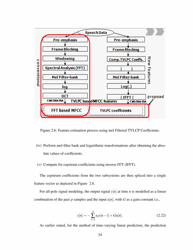
Figure 2.6: Feature estimation process using mel Filtered TVLCP Coefficients.

(iv) Perform mel-filter bank and logarithmic transformations after obtaining the abso-

lute values of coefficients.

(v) Compute for cepstrum coefficients using inverse FFT (IFFT).

The cepstrum coefficients from the two subsystems are then spliced into a single

feature vector as depicted in Figure 2.6.

For all-pole signal modeling, the output signal y[n] at time n is modelled as a linear

combination of the past p samples and the input u[n], with G as a gain constant i.e.,

y[n] =−p

∑i=1

aiy[n− i]+Gu[n]. (2.22)

As earlier stated, for the method of time-varying linear prediction, the prediction

34

coefficients are allowed to change with time progress [29]. Once more, the time-varying

model can be represented by

y[n] =−p

∑i=1

ai[n]y[n− i]+Gu[n]. (2.23)

From equation (5.2), we assume

ai[n] = a1,i +a2,i(n), (2.24)

then

y[n] =−p

∑i=1

(a1,i +a2,i(n))y[n− i]+Gu[n]. (2.25)

If

Y (z−1) =∞

∑i=0

y(i)z−i,

U(z−1) =∞

∑i=0

u(i)z−i, and

δY (z−1)

δ z=

∞

∑i=0

y[i](−i)z−i−1; (2.26)

then Y(z−i) =−∑pi=1 a1,iz−i.Y (z−i)+∑

pi=1 a2,iz−i.δY (z−i)

δ z +

GU(z−i).

Subsequently,

(1+p

∑i=1

a1,iz−i)Y (z−1)−p

∑i=1

a2,iz−i δY (z−1)

δ z= GU(z−1). (2.27)

Let,

A1(z−1)Y (z−1)−A2(z−1)δY (z−1)

δ z= GU(z−1), (2.28)

where,

35

A1(z−1)Y (z−1) is the time-invariant component and −A2(z−1)δY (z−1)δ z is the time

varying component.

If the time invariant component is the dominant factor, the time invariant component

transfer function can be approximately obtained as follows,

A1(z−1)Y (z−1) = GU(z−1), (2.29)

H1(z−1) =1

A1(z−1). (2.30)

However, if the time varying component is the dominant factor, then the time varying

component transfer function can be approximately obtained as follows

−A2(z−1)δY (z−1)

δ z= GU(z−1), (2.31)

H2(z−1) =1

A2(z−1)=

(1

a2,1

)1

1+∑pi=2

a2,i+1a2,1

z−i, (2.32)

which can be represented as

H2(z−1) =b0

1+∑p−1i=1 biz−i

, (2.33)

where b0 =1

a2,1, and bi =

a2,i+1a2,1

.

converting from frequency to Mel scale is achieved using

mel( f ) =

1125ln(1+ f

700) if f>1kHz

f if f<1kHz

(2.34)

where mel( f ) is the Mel-frequency scale and f is the linear frequency. The purpose of

the Mel-filter bank is to filter the magnitude spectrum that is passed to it and to give

an array output called Mel-spectrum. Each of the values in the Mel-spectrum array

corresponds to the result of the filtered magnitude spectrum through the individual Mel-

filters. The mel filter banks are calculated as

36

Wmel(k) =

0 k < f (m−1)

k− f (m−1)f (m)− f (m−1) f (m−1)6 k 6 f (m)

f (m+1)−kf (m+1)− f (m) f (m)6 k 6 f (m+1)

0 k > f (m+1)

(2.35)

where Wmel represent the triangular weighting function associated with kth mel band

in the mel scale and the Mel-spectrum is given by

Yi(n) =K−1

∑k=0|bi(k)|.Wmel(n,k) (2.36)

where, K is number of frames, k is frame index, n = 0,1,2, ...,M−1 is mel-filter index

and M is number of mel-filters. TVLPC based MFCC features are computed by taking

the log of the mel-spectrum Yi(n) and computing the inverse fast Fourier transform as

Ci =1N

N−1

∑n=0

[logYi(n)

]e

2π jN ni (2.37)

2.2.4 Influence of TVLPC coefficient gain

We compute the coefficients gain of time-varying components of the proposed approach.

In the case of speech features estimated by mel filtered TVLPC based MFCC features,

the gain is used as a benchmark in determining whether Equation (5.8) or (5.10) should

be used in obtaining features in the proposed method. The same gain serves a purpose

of checking the presence of variability in intra-frame coefficients. In addition

if log |b0|> 0, c′i = ci

otherwise < 0, c′i = 0.

. (2.38)

37

where ci is the TVLPC based MFCCs features. If gains are mostly large (positive) it

confirms that time-varying is dominant and should be considered, otherwise only time

invariant features should be considered.

The simulations are based on speech analysed using triangular mel filtered time

varying linear predictive coefficients (TVLPC) of an auto-regressive model with pre-

emphasis but without windowing. A speech segment, 128 samples (11.6ms) per frame

of 7 frames, is extracted from the speech signal of each phrase, post voice activity de-

tection (VAD) using short term energy and zero-crossing rate respectively. The VAD

process eliminates silent parts. The time-varying LPC gain for each frame in the speech

segment is then computed.

Shown in Figures 2.7, 2.8, and 2.9, are waveforms and time-varying LPC gains based

on mel filtered TVLPC coefficients for three Japanese phrases; “genki”, “denki” and

“tenki”. This computation process is done with the aim of validating the effectiveness

Figure 2.7: Waveform for 7 frames of a Japanese phrase /genki/ after VAD and pre-

emphasis and magnitude spectrum of normalized tvLPC coefficients frame-by-frame.

of the proposed approach (i.e., by determining the presence of intra-frame variations) in

differentiating similar speech phrases. The top graph in Figure 2.7 shows a waveform

for “genki” while shown immediately below is the frame-by-frame tvLPC gain graph.

38

Figure 2.8: Waveform for 7 frames of a Japanese phrase /denki/ after VAD and pre-

emphasis and magnitude spectrum of normalized tvLPC coefficients frame-by-frame.

Figure 2.9: Waveform for 7 frames of a Japanese phrase /tenki/ after VAD and pre-

emphasis and magnitude spectrum of normalized tvLPC coefficients frame-by-frame.

Figure 2.8 and Figure 2.9 show the comparative results for “denki” and “tenki” in the

same order respectively.

39

2.3 Proposed feature model

The selection of an adequate feature vector for signal detection and a robust decision rule

is a challenging problem that affects the performance of voice activity detector (VAD)

working under noise conditions. This entails a need for noise robust speech features.

In order to achieve such features, the frond-end system should be designed with precise

and robust algorithms. In attempting to achieve such features, we begin by defining the

feature models.

2.3.1 Definition of models

We formulate thirteen models, models 0 to 12 of feature vectors. In this study, models

are formulated as follows: First, model 0 makes use of fast Fourier transform (FFT)-

based MFCC only and is referred to as a conventional method. Models 1 to 12 are

formulated as follows: FFT based MFCC coefficients consisting of 38-dimensional fea-

ture vectors are concatenated with TVLPC based MFCC coefficients. The number of

TVLPC-based MFCC coefficients appended to FFT-based MFCC coefficients indicate

the proposed model number. For example, appending a single TVLP-based MFCC

coefficient to 38 coefficients of FFT-based MFCC make up model 1 and appending

2 TVLPC-based MFCC coefficients to 38 coefficients of FFT-based MFCC make up

model 2 and so on. Therefore, in model 12, 12 of TVLPC-based MFCC coefficients are

appended to the 38 cepstrum coefficients of model 0. The model definition is as fol-

lows: The model 0 is considered as a conventional approach (using FFT-based MFCC

features only) and its 38-parameter feature vector consisting of 12 cepstral coefficients

(without the zero-order coefficient) plus the corresponding 13 delta and 13 acceleration

coefficients is given by [b1b2 . . .b12∆b0∆b1 . . .∆b12∆2b0∆2b1 . . .∆2b12] where bi, ∆bi and

40

∆2bi, are MFCC, delta MFCC and delta-delta MFCC, respectively. As for the proposed

models, j( j = 1, . . . ,12) , we append the intra-frame cepstrum for time-varying coeffi-

cients [c11,c

12, . . . ,c

1j ] to the model 0 feature vector depending on the model number as

shown in Figure 2.10 and depicted in Figure 2.11. Given that the number of time-

Figure 2.10: Proposed concatenated speech features, with model 0 as conventional ap-

proach.

varying LP cesptrum coefficients appended to Model 0 represent the model number, it

therefore, means that model 0 has none time-varying LP cepstrum coefficient appended

to it.

2.4 Feature classification techniques

Two major steps in ASR are speech feature extraction and feature matching. Speech

recognition involves comparing speech features of known and unknown speech signal

in order to determine their similarity. According to the specifics of recognition system,

speech feature comparison can be done using different approaches [62]. Usually the

41

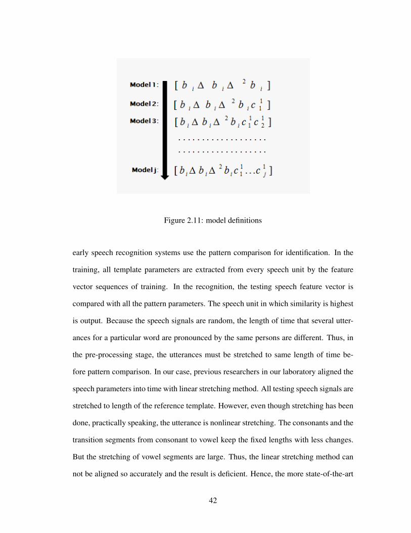
Figure 2.11: model definitions

early speech recognition systems use the pattern comparison for identification. In the

training, all template parameters are extracted from every speech unit by the feature

vector sequences of training. In the recognition, the testing speech feature vector is

compared with all the pattern parameters. The speech unit in which similarity is highest

is output. Because the speech signals are random, the length of time that several utter-

ances for a particular word are pronounced by the same persons are different. Thus, in

the pre-processing stage, the utterances must be stretched to same length of time be-

fore pattern comparison. In our case, previous researchers in our laboratory aligned the

speech parameters into time with linear stretching method. All testing speech signals are

stretched to length of the reference template. However, even though stretching has been

done, practically speaking, the utterance is nonlinear stretching. The consonants and the

transition segments from consonant to vowel keep the fixed lengths with less changes.

But the stretching of vowel segments are large. Thus, the linear stretching method can

not be aligned so accurately and the result is deficient. Hence, the more state-of-the-art

42

pattern comparison techniques are considered in this study.

2.4.1 Artificial neural networks

Artificial neural networks(ANNs) are used to calculate or approximate functions that

may depend on a large number of unknown inputs. Artificial neural networks are rep-

resented as system of “neurons” which are interconnected and send messages to each

other. The connections have numeric weights that can be assigned or turned on expe-

rience, thus making neural nets adaptive to the inputs and capable of learning. ANNs

inspired by biological neural networks i.e the central nervous systems of animals, in

particular the brain, are a family of statistical learning models [63] composed of simple

elements operating in parallel. The elements are inspired by biological nervous systems.

Like in nature, the network function is determined largely by the connections between

elements. We can train a neural network to perform a particular function by adjusting

the values of the connections (weights) between elements. Commonly, neural networks

are adjusted, or trained, so that a particular input leads to a specific target output. An

artificial Neural Network is used as recognition and identification method. The network

has varying neurons input n, which receive input of front-end feature extraction system.

Number of hidden layer varies from 1 to 4 layers and number of neurons in each hidden

layer varies from 10 to 50 neurons.

The basic architecture of a general neural network will be divided into three types

of layers - input, hidden, and output. The signal will flow stringently in a feed forward

direction from input to output.

Neural networks have been trained to perform complex functions in various fields

of application including pattern recognition, identification, classification, speech, vi-

sion, and control systems. In recent times neural networks have been trained to solve

43

problems that are difficult for conventional computers or human beings. In some cases,

neural network pattern recognition tools (NPR tools) are used. Such tools perform su-

pervised training and testing [64].

2.4.2 Hidden Markov model method

According to Juan and colleagues [45], in speech, like in pattern recognition, the main

objective is not to obtain extremely representative models, but to eliminate recognition

errors. The hidden Markov model (HMM) [8, 65–67] is where the speech signal can

be well characterized as a double parametric random processes. One process is used to

describe the statistical method of characterizing the spectral properties of the short-time

nonstationary signal (or instantaneous character of signals), while the other process is

used to describe the process of how a short-time stationary signal is made to transi-

tion to the next short-time stationary signal, as well as dynamic character of the speech

signal. Based on the double random processes, HMM approach can identify the short-

time stationary speech signals of difference parameter. It can also follow the process of

transition between these speech signals.

The human’s process of speech also is a double stochastic processes. The speech

signal is an observable sequence. It is the parameters sequences that the brain makes into

phonemes, words or sentences by the grammar and human’s minds. Thus the parameters

sequences is unobservable. Many experiments have shown that the HMM approach can

describe the processing of phonation of speech signal very accurately.

All parameters of the HMM are defined as follows.

(1) N is the number of states in the model. Although the states are hidden, for many

practical applications there is often some physical significance attached to the sates or

to sets of states of the model. The individual states are labeled as {1,2, . . . ,N}, qi is the

44

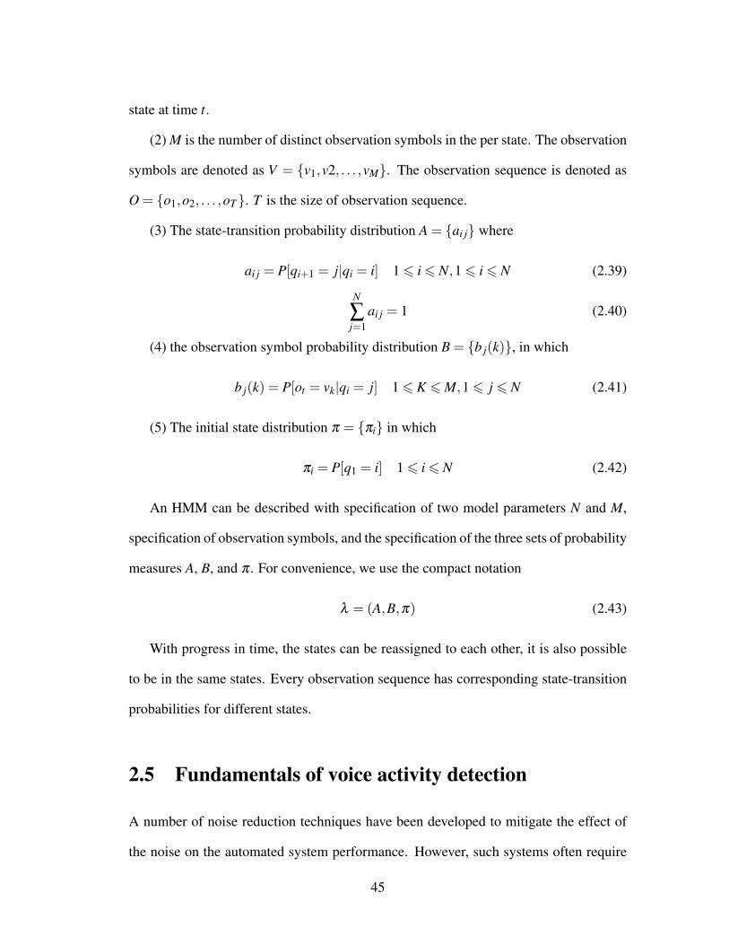
state at time t.

(2) M is the number of distinct observation symbols in the per state. The observation

symbols are denoted as V = {v1,v2, . . . ,vM}. The observation sequence is denoted as

O = {o1,o2, . . . ,oT}. T is the size of observation sequence.

(3) The state-transition probability distribution A = {ai j} where

ai j = P[qi+1 = j|qi = i] 1 6 i 6 N,1 6 i 6 N (2.39)

N

∑j=1

ai j = 1 (2.40)

(4) the observation symbol probability distribution B = {b j(k)}, in which

b j(k) = P[ot = vk|qi = j] 1 6 K 6 M,1 6 j 6 N (2.41)

(5) The initial state distribution π = {πi} in which

πi = P[q1 = i] 1 6 i 6 N (2.42)

An HMM can be described with specification of two model parameters N and M,

specification of observation symbols, and the specification of the three sets of probability

measures A, B, and π . For convenience, we use the compact notation

λ = (A,B,π) (2.43)

With progress in time, the states can be reassigned to each other, it is also possible

to be in the same states. Every observation sequence has corresponding state-transition

probabilities for different states.

2.5 Fundamentals of voice activity detection

A number of noise reduction techniques have been developed to mitigate the effect of

the noise on the automated system performance. However, such systems often require

45

an estimate of the noise statistics obtainable by means of a precise voice activity detector

(VAD) [68]. Speech and non-speech detection is a complex problem that affects numer-

ous applications including mobile communication services [69], real-time speech trans-

mission on the Internet [70] or noise reduction for digital hearing aid devices [71]. For

example, a VAD achieves silence compression in modern mobile telecommunication

systems reducing the average bit rate by using the discontinuous transmission (DTX)

mode.

The different VAD methods include those based on energy thresholds [70], pitch

detection [72], spectrum analysis [73], zero-crossing rate [74] [75], periodicity mea-

sure [76], or combinations of different features [77]. Figure 2.12 shows the waveforms

for a Japanese phrase /genki/ before and after short term energy VAD. The periodicity

is more clear after applying VAD. Desirable aspects of VAD algorithms include a good

Figure 2.12: Short Term energy contour of a Japanese speech phrase /genki/

46

decision rule, adaptability to background noise as well as low computational complexity

[70]. Most of the VADS that formulate the decision rule on a frame by frame basis nor-

mally use decision smoothing algorithms in order to improve the robustness against the

noise. The motivations for these approaches are found in the speech production process

and the reduced signal energy of word beginnings and endings.

In the robust speech recognition, among many intentions of VAD are the following:

(i) Detecting the speech frame and background noise from the signal of speech frame.

The VAD can influence the performance of ASR. If the speech segment is recog-

nized to be noise, then some important speech data are lost and the recognition

accuracy is decreased. Similarly, if the noise segment is recognized to be speech,

then calculation cost and the error probability of comparison with reference pat-

terns will be raised, the recognition accuracy is also decreased.

(ii) Reducing the computational cost. The computational cost is significant to low

performance hardware, mobile device or embedded systems. The VAD can trim

the nonspeech segments and abridge the speech coding, then the ASR system can

not only improve the recognition performance but also time.

(iii) Some speech recognition algorithms require estimate of the spectrum character-

istics of noise. The spectral subtraction (SS), e.g., the spectrum characteristics of

noise is estimated with the detected noise.

2.6 Effects of noise on speech

Automatic speech recognition (ASR) is one of the dominant automation serving as a

man-to-machine admix for real-world applications. In general, the performance of an

47

ASR system is usually degraded when there exist environmental mismatches between

training and test phases [78]. The main causes of speech variation in real environments

are the various kinds of background noises that affect the feature extraction stage in an

ASR system [19]. In this sense, the front-end for robust speech recognition requires to

reduce redundancy and inconstancy as well as the ability to capture important cues of

speech signals, even in noisy environments.

2.6.1 Noise data

The 15 types of noises used in our experiments are based on Signal Processing Infor-

mation Base (SPIB) noise data measured in field by Speech Research Unit (SRU) at

Institute for Perception-TNO, Netherlands, United Kingdom, under the project number

2589-SAM (Feb. 1990) [79]. The names and brief descriptions of the noises are;

1. White Noise: acquired by sampling a high-quality analog noise generator (Wandel

Goltermann), which results in equal energy per Hz bandwidth.

2. Pink Noise: acquired by sampling a high-quality analog noise generator (Wandel

Goltermann), yielding equal energy per 1/3 octave.

3. HF Channel Noise: acquired from an HF radio channel after demodulation.

4. Speech Babble: acquired by recording samples from 1/2” BK condensor micro-

phone onto digital audio tape (DAT). The source of this babble is 100 people

speaking in a canteen. The room radius is over two meters; therefore, individual

voices are slightly audible. The sound level during the recording process was 88

dBA.

5. Factory Floor Noise 1: acquired by recording samples from 1/2” BK condensor

48

microphone onto digital audio tape (DAT). This noise was recorded near plate-

cutting and electrical welding equipment.

6. Factory Floor Noise 2: acquired by recording samples from 1/2” BK condensor

microphone onto digital audio tape (DAT). This noise was recorded in a car pro-

duction hall.

7. Cockpit Noise 1 (Buccaneer Jet Traveling at 190 knots): acquired by recording

samples from 1/2” BK condensor microphone onto digital audio tape (DAT). The

Buccaneer jet was moving at a speed of 190 knots, and an altitude of 1000 feet,

with airbrakes out. The sound level during the recording process was 109 dBA.

8. Cockpit Noise 2 (Buccaneer Jet Traveling at 450 knots): acquired by recording

samples from 1/2” BK condensor microphone onto digital audio tape (DAT). The

Buccaneer was moving at a speed of 450 knots, and an altitude of 300 feet. The

sound level during the recording process was 116 dBA.

9. Engine Room Noise (Destroyer engine): acquired by recording samples from mi-

crophone onto digital audio tape (DAT). The sound level during the recording

process was 101 dBA.

10. Operations Room Background Noise (Destroyer operations): acquired by record-

ing samples from microphone onto digital audio tape (DAT). The sound level

during the recording process was 70 dBA.

11. Cockpit Noise 3 (F-16): acquired by recording samples from 1/2” BK condensor

microphone onto digital audio tape (DAT). The noise was recorded at the co-

pilot’s seat in a two-seat F-16, traveling at a speed of 500 knots, and an altitude of

300-600 feet. The sound level during the recording process was 103 dBA. It was

49

found that the flight condition had only a minor effect on the noise and, therefore,

the reproduced noise can be considered to be representative.

12. Military Vehicle Noise (Leopard): acquired by recording samples from 1/2” BK

condensor microphone onto digital audio tape (DAT). The Leopard 1 vehicle was

moving at a speed of 70 km/h. The sound level during the recording process was

114 dBA.

13. Military Vehicle Noise (M109): acquired by recording samples from 1/2” BK

condensor microphone onto digital audio tape (DAT). The M109 tank was moving

at a speed of 30 km/h. The sound level during the recording process was 100 dBA.

14. Machine Gun Noise: acquired by recording samples from 1/2” BK condensor

microphone onto digital audio tape (DAT). The weapon used was a .50 calibre

gun fired repeatedly.

15. Vehicle Interior Noise (Volvo 340): acquired by recording samples from 1/2” BK

condensor microphone onto digital audio tape (DAT). This recording was made at

120 km/h, in 4th gear, on an asphalt road, in rainy conditions.

Performance of ASR systems operating in noisy environments normally declines and

non efficient speech/non-speech detection appears to be an important degradation source.

In most researches of speech recognition, the standard practice is to record speech

databases in relatively quiet environments. Thus, the better recognition accuracy can be

obtained with the recognition system that speeches are trained or created to reference

models in a controlled quite environment. As for the application of speech recognition

system, the recognition environment is more complex. Under real (uncontrolled) noise

environment, the recognition performance is drastically lower because there is a dis-

crepancy between the feature vectors of the noisy speeches and the reference models,

50

which are created under controlled environment [80–82]. Figure 2.13 demonstrates the

negative effects of noise on speech. The figure shows a segment of clean speech and

Figure 2.13: The effects of increased babble noise on Japanese speech segment /genki/

effects of babble noise at 20 dB, 10 dB and 0 dB respectively on a Japanese speech

phrase /genki/. The deterioration of speech phrase, by amplitude reduction, can easily

be observed with increase in noise from 20 dB to to 0 dB.

Figure 2.14(a) shows the effects of noise on both spectrum and cepstrum domains

on a clean Japanese speech phrase /genki/. Figure 2.14(b) , 2.14(c) and 2.14(d) show

effects of babble noise in spectrum and cespstrum domains on Japanese speech phrase

/genki/ at 20 dB , 10 dB and 0 dB SNR respectively. It can, clearly be seen that , just

like in the case of time domain speech waveform, the spectrum domains as well as the

cepstrum domains of speech are equally distorted with increase in noise.

Figure 2.15 shows the distributive effects of white noise on speech signal. It shows

the power spectrum of a clean Japanese speech phrase /tenki/ and a noisy speech phrase

at 10 dB white noise.

51

(a) (b)

(c) (d)

Figure 2.14: (a) The waveform, spectrum and cepstrum of clean speech /genki/ (b)

Spectrum and Cepstrum with babble noise at 20 dB, (c) Spectrum and Cepstrum with

babble noise at 10 dB (d) Spectrum and Cepstrum with babble noise at 0 dB SNR

The result goes to demonstrate the significance of reduction techniques to mitigate

the noise effects even in cases where VAD is applied.

The robust noisy speech recognition has been a research focus in the last twenty

years, the researches proposed many ways aimed at improving the performance of ASR

system. But any perfect solution has not been proposed for robust ASR system. The

major influences emanate from a number of factors including the following:

(i) The influence of double articulation. The acoustic feature of speech signal is

closely related with the pronounciation. The acoustic features of speech signal

52

(a) (b)

Figure 2.15: (a) The power spectrum of clean speech /tenki/ (b) power spectrum with

white noise at 10 dB SNR

may be made a great deal of different in different contexts and characterizes some

language constructions. Moreover, two same utterances may express different

meanings.

(ii) The influence of language complexity. The meaning of a sentence is closely re-

lated with the contexts and cultural background. Furthermore, the structure of

sentence is variation in language grammar. But it is very difficult that the infor-

mation of context are applied to ASR.

(iii) The influence of variation of pronunciation for speaker himself. For the factors of

age, sentiment, health condition, speaking speed and so on, the acoustic features

are different between utterances of same word.

(iv) The influence of utterances for different speakers. The utterances between differ-

ent speakers have big difference, because their vocal cords are different.

(v) The influence of ambient environment. The speech signal can be distorted easily

by the noise, reverberation, microphone, transmission channel and many other

53

environmental related sources of disturbances.

Noise reduction techniques are aimed at reducing the noise and extracting the real

speech from the noisy speech. They possibly attempt to increase the acoustic feature of

real speech signal, in order to improve the recognition accuracy of ASR system. The

enhancement mostly takes place in the cepstral domain as discussed later.

54

Chapter 3

Voice Activity Detection

3.1 VAD fundamentals

The performance of most of the speech processing systems is degraded by convolutional

and environmental noises both of which can jointly be removed, prior to recognition,

through feature enhancement techniques [83]. Other techniques include use of Tay-

lor series [84], RASTA [85], and by using admix of RASTA-PLP [86] among many

other methods. Despite the much progress made in this research area, a number of tech-

nical challenges still inhibit automated systems from meeting the modern applications

demands especially in speech recognition [68]. Numerous noise reduction techniques

often require an estimate of the noise statistics obtained by means of a precise voice

activity detector (VAD).

An important problem in many areas of speech processing is the determination of

presence of speech periods in a given signal. This task can be identified as a statistical

hypothesis problem whose main purpose is determining to which category or class a

given signal belongs. This classification task is non trivial since the increasing level of

background noise degrades the classifier effectiveness.

55

The human’s speech is incohesive. Thus, the ASR system becomes effective once

speech is detected. Usually, only the voice activity detection (VAD) algorithm is in

execution in order to reduce the computation cost of ASR system, when speech signal

is insignificant. Furthermore, the accurate detection of speech begin and endpoints is

important in order to improve the recognition accuracy of ASR system. Thus, VAD is a

very important technique problem, especially in high ambient noise environments. The

accurate endpoint detection of speech is a simple problem in the most favorable envi-

ronments. Therefore, VADs are frequently used in a number of applications including

speech coding, speech enhancement and speech recognition. A precise VAD extracts

a set of discriminative speech features from the noisy speech and formulates the deci-

sion in terms of well defined rule. In practice, however, one or more problems usually

arise that make accurate VAD challenging, particularly in such speech-correlated noise

as reverberation and reflection as well as in an uncorrelated (additive which includes

both stationary and unstationary) noise. VAD may also prove uneffective in nonsta-

tionary environments (e.g., the presence of door slams, irregular road noise, car horns,

irregular conversations) coupled with speech interference (as from TV, radio, thermal

appliances). Other noise contributing factors are the distortion introduced by such input

equipment as microphone (transmitter), distance to the microphone, filter, transmission

system when the speech is sent, (e.g., distortion, noise, echo, etc.) and distortions from

the recording equipment [87]. In this regard, many VAD methods have been proposed

in speech recognition systems.

VAD algorithm typically relies on the short-time energy and zero-crosssing rate

[88]. The associated techniques use different features of syllables in the time-domain

and have a low computational complexity. In this chapter, we later discuss these kinds

of VAD and propose the VAD algorithm for our study experiments.

56

3.2 Short-time energy algorithm

The first natural division of all signals is into either stationary or non-stationary cate-

gories. Stationary signals are constant in their statistical parameters over time. If you

look at a stationary signal for a few moments and then wait an hour and look at it again,

it would look essentially the same, that is, its overall level would be about the same

and its amplitude distribution and standard deviation would be about the same. Rotating

machinery generally produces stationary vibration signals. Stationary signals are fur-

ther divided into deterministic and random signals. Random signals are unpredictable

in their frequency content and their amplitude level, but they still have relatively uni-

form statistical characteristics over time. Examples of random signals are rain falling

on a roof, jet engine noise, turbulence in pump flow patterns and cavitation [89].

Speech is produced from a time varying vocal tract system with time varying ex-

citation. As a result, the speech signal is non-stationary in nature. Most of the signal

processing tools studied in signals and systems and signal processing assume time in-

variant system and time invariant excitation, i.e. stationary signal. Since the speech

signal is nonstationary in nature, the way stationary signal is processed cannot be used

to process a speech signal. Thus a need for a different way of processing speech.

An engineering solution proposed for processing speech was to make use of existing

signal processing tools in a modified fashion. To be more specific, the tools can still

assume the signal under processing to be stationary. Speech signal may be stationary

when it is viewed in blocks of 10∼ 30 ms. Hence to process speech by different signal

processing tools, it is viewed in terms of 10 ∼ 30 ms. Such a processing is termed as

Short Term Processing (STP).

The speech signal in 10∼ 30 ms time can be as a quasi-steady signal (as short-time

steady state), because the parameters of spectrum and physical characteristics are almost

57

invariant [42, 90].

Therefore, a speech signal can be partitioned into many short frames and each frame

is as a detecting unit. According to the energies of speech and nonspeech frame, short-

time energy based VAD approach can identify endpoints of any speech signal, because

the energy associated with voiced region is large compared to unvoiced region and si-

lence region will have least or negligible energy [91–94]. Thus short term energy can

be used for voiced, unvoiced and silence classification of speech.

Short Term Processing (STP) of speech can be performed either in time domain or

in frequency domain. The particular domain of processing depends on the information

from the speech that we are interested in. For instance, parameters like short term en-

ergy, short term zero crossing rate and short term autocorrelation can be computed from

the time domain processing of speech. Alternatively, short term Fourier transform can

be computed from the frequency domain processing of speech. Each of these parameters

give different information about speech that can be used for automatic processing.

The samples of a waveform of input speech signal is defined as x(m), m is the sample

index. The short-time square energy of speech signal Esqr(n) is defined as

Esqr(n) =+∞

∑m=−∞

[x(m)ω(m−n)]2. (3.1)

This measurement can in a way be used in distinguishing between voiced and unvoiced

segments, since unvoiced speech has significantly smaller short-term energy. For The

length of the window a practical choice is 10 ∼ 30 ms that is 160 ∼ 320 samples for

sampling frequency 16kHz. This way the window will include a suitable number of

pitch periods so that the result will be neither too smooth nor too detailed. The short-

time average amplitude Eavg(n) is defined as

Eavg(n) =+∞

∑m=−∞

|x(m)|ω(m−n). (3.2)

58

The average magnitude calculation does not emphasize large signal levels so much as

short-time energy since its calculation does not include squaring.

The short-time logarithm energy Elog(m) is defined as

Elog(n) =+∞

∑m=−∞

log[x(m)ω(m−n)]2. (3.3)

The ω(n) is the window function which is small width in samples, it represents the

frame size n. Usually the rectangular, Hamming and Hanning window functions are

used in speech signal processing. The rectangular window function is defined as

ω(n) =

{1 0 6 n 6 N−1

0 other.(3.4)

The Hamming window function is defined as

ω(n) =

{0.54−0.64cos( 2nπ

N−1) 0 6 n 6 N−1

0 other.(3.5)

The Hanning window function is defined as

ω(n) =

{0.5(1− cos( 2nπ

N−1)) 0 6 n 6 N−1

0 other.(3.6)

The short-time square energy Esqr(n), logarithm energy Elog(n), and average ampli-

tude Eavg(n) can all embody the signal strength, but their characteristics are different.

To embody the dynamic range of amplitude, the Eavg is better than Esqr and Elog. To

embody the level difference between unvoiced and consonants, the Eavg is worse than

Esqr and Elog. Hence we use the short-time square energy Esqr and hanning window

function to detect endpoint in the chapter.

59

3.3 Short term autocorrelation algorithm

In signal processing, cross-correlation can be used for finding the similarity among the

two sequences and refers to the case of having two different sequences for correlation.

On the other hand, autocorrelation refers to the case of having only one sequence for

correlation. In autocorrelation, the interest is in observing how similar the signal char-

acteristics is with respect to time. Autocorrelation is a mathematical tool for finding

repeating patterns, such as the presence of a periodic signal obscured by noise. This is

achieved by providing different time lag for the sequence and computing with the given

sequence as reference.

The autocorrelation is a very useful tool in case of speech processing. However due

to the non-stationary nature of speech, a short term version of the autocorrelation is

often needed. The autocorrelation of a stationary sequence rxx(k) is given by

rxx(k) =∞

∑m=−∞

x(m).x(m+ k) (3.7)

The corresponding short term autocorrelation of a non-stationary sequence s(n) is

defined as

rss =∞

∑m=−∞

sw(m).sw(k+m)rss(n,k) =∞

∑m=−∞

(s(m)w(n−m).s(k+m).w(n− k+m))

(3.8)

where sw(n) = s(m).w(n−m) is the windowed version of s(n). Thus for a given win-

dowed segment of speech, the short term autocorrelation is a sequence. The nature of

short term autocorrelation sequence is primarily different for voiced and unvoiced seg-

ments of speech. Hence information from the autocorrelation sequence can be used for

discriminating voiced and unvoiced segments.

60

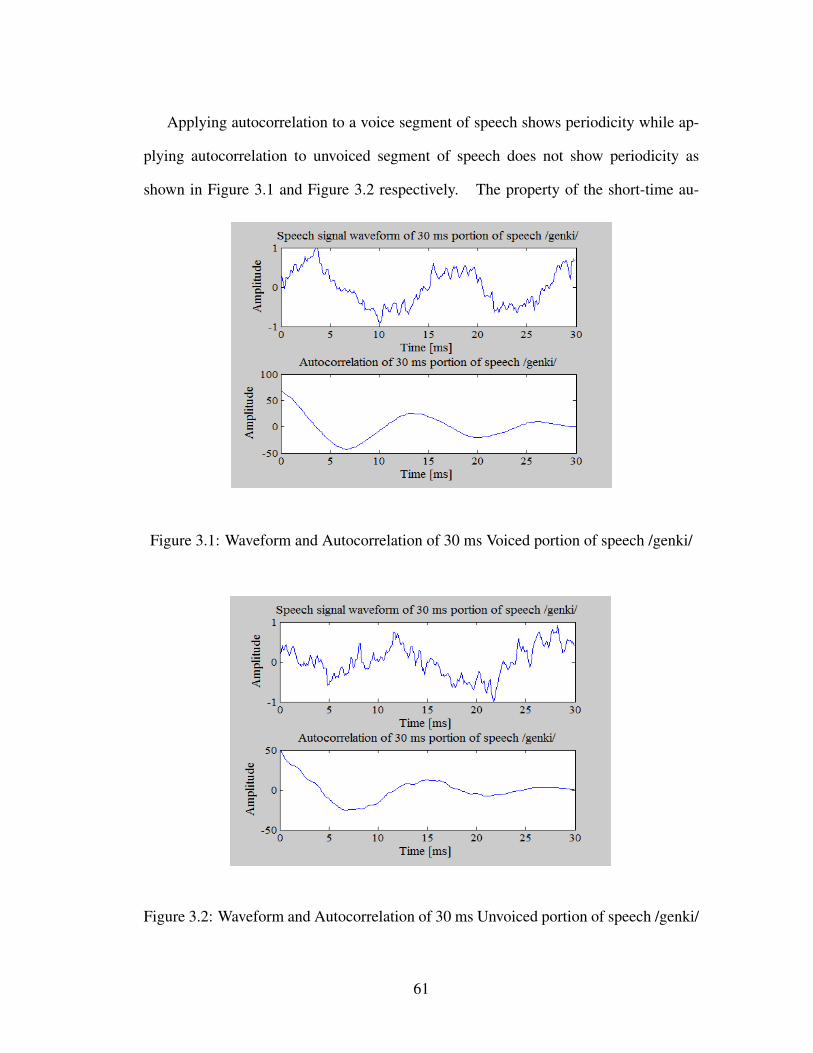
Applying autocorrelation to a voice segment of speech shows periodicity while ap-

plying autocorrelation to unvoiced segment of speech does not show periodicity as

shown in Figure 3.1 and Figure 3.2 respectively. The property of the short-time au-

Figure 3.1: Waveform and Autocorrelation of 30 ms Voiced portion of speech /genki/

Figure 3.2: Waveform and Autocorrelation of 30 ms Unvoiced portion of speech /genki/

61

tocorrelation to reveal periodicity in a signal is demonstrated. Periodicity can be defined

as perpetually spaced frequencies. We note how the autocorrelation of the voiced speech

segment retains the periodicity. On the other hand, the autocorrelation of the unvoiced

speech segment looks more like noise. In general, autocorrelation is considered as a

robust indicator of periodicity.

3.4 Zero-crossing rate algorithm

Sometimes, as earlier indicated short-time energy algorithms are not accurate for VAD

under noisy conditions. The human’s pronunciation include the unvoiced and voiced.

The voiced is produced by the vibration of the vocal chords. The amplitude of voiced

is high and periodicity is apparently. The unvoiced is without vibration of the vocal

chords, it is produced by the friction, impact or plosive that the suction of air into the

mouth. Thus, the short-time energy is lower than that of voiced. It can be identified

into nonspeech easily by short-time energy method. The amplitude of unvoiced seg-

ment is lower than that of voiced segment, and it is almost same to that of nonspeech

segment. Hence, they are very difficult to identify with just our eyes. If the nonspeech

and unvoiced segments are zoomed, we discover that the waveform of unvoiced seg-

ment fluctuates so quickly around zero level value, and the number of crossing zero

level value for nonspeech segment is fewer. The zero crossing rate can help improving

the VAD under noisy conditions.

Let w be the window, and n be the sample that the window is centred on, with N

being the window size. We denote sgn[] as the sign number function and x(n) as the

discrete audio signal. The zero crossing rate is the rate at which the signal changes i.e.

62

goes from negative to positive and vice versa. The zero-crossing rate is defined as

ZCR(n) =12

+∞

∑m=−∞

|sgn[x(m)]− sgn[x(m−1)]|ω(m−n), (3.9)

where the sgn[·] is symbol function, it is defined as

sgn[x] =

{1 x > 0

−1 x < 0(3.10)

The ω(n) usually uses the rectangular window function.

Figures 3.3, 3.4, and 3.5 show the waveform, short-time energy and zero-crossing

rate of frames for a clean Japanese speech phrase “genki” respectively.

Figure 3.3: Waveform of word of clean speech /genki/

Figure 3.6, Figure 3.7 and Figure 3.8 show the waveform, short-time energy and zero-

crossing rate of frames for a noisy Japanese speech phrase “genki” at 10 dB white noise

respectively. The number of crossing zero level value can be used to distinguish the

endpoint of speech signal. The method is described as zero-crossing rate (ZCR) [95–98].

63

Figure 3.4: Short-time energy of frames of clean speech phrase /genki/

Figure 3.5: Zero-crossing rate of frames of clean speech phrase /genki/

64

Figure 3.6: Noisy speech signal at 10 dB

Figure 3.7: Short-time energy of frames of a noisy speech signal at 10 dB SNR

65

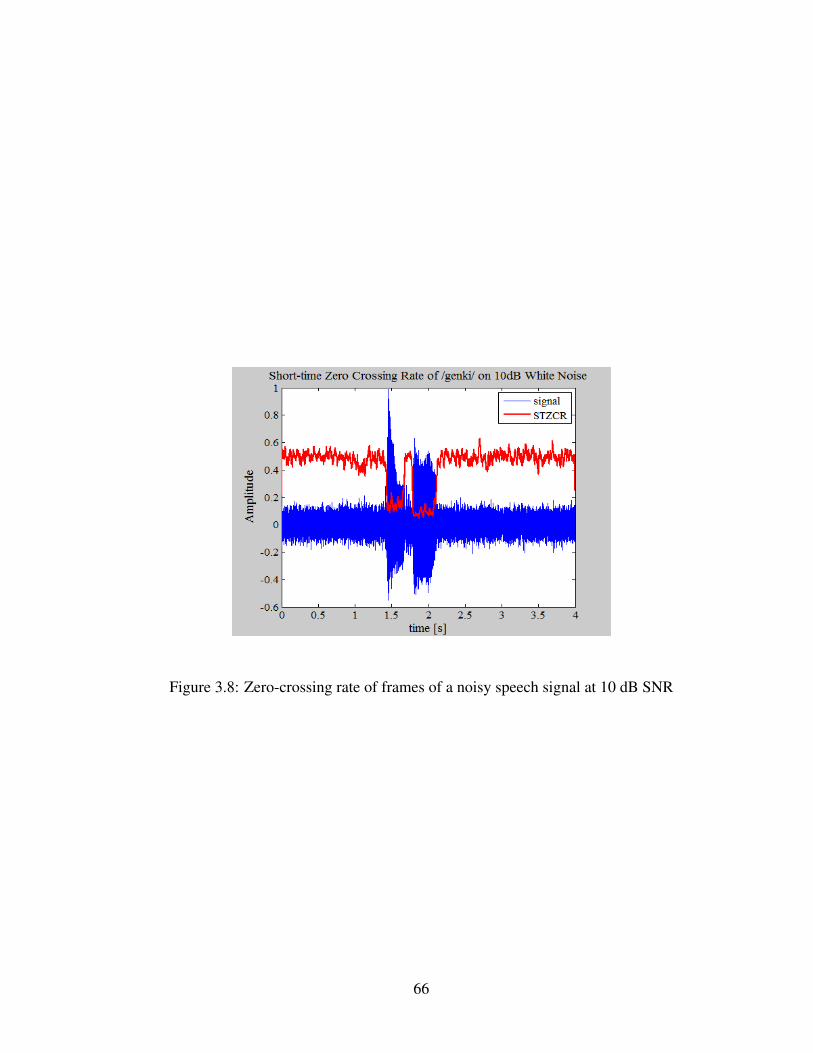
Figure 3.8: Zero-crossing rate of frames of a noisy speech signal at 10 dB SNR

66

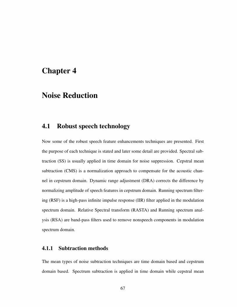
Chapter 4

Noise Reduction

4.1 Robust speech technology

Now some of the robust speech feature enhancements techniques are presented. First

the purpose of each technique is stated and later some detail are provided. Spectral sub-

traction (SS) is usually applied in time domain for noise suppression. Cepstral mean

subtraction (CMS) is a normalization approach to compensate for the acoustic chan-

nel in cepstrum domain. Dynamic range adjustment (DRA) corrects the difference by

normalizing amplitude of speech features in cepstrum domain. Running spectrum filter-

ing (RSF) is a high-pass infinite impulse response (IIR) filter applied in the modulation

spectrum domain. Relative Spectral transform (RASTA) and Running spectrum anal-

ysis (RSA) are band-pass filters used to remove nonspeech components in modulation

spectrum domain.

4.1.1 Subtraction methods

The mean types of noise subtraction techniques are time domain based and cepstrum

domain based. Spectrum subtraction is applied in time domain while cepstral mean

67

subtraction is applied in cepstrum domain.

4.1.1.1 Spectral Subtraction (SS)

Spectrum Subtraction (SS) method assumes that the noise and speech are uncorrelated

and additive in the time domain. The method also assumes that the noise character-

istics change slowly relative to those of speech signals, such that the noise spectrum

estimated during a non-speech period can be used for suppressing the noise contaminat-

ing the speech. SS reduces DC components of modulation spectrum which corresponds

to power spectrum [99]. The method is simple and efficient for stationary or slowly

varying wide-band additive noise, but with some challenges. For example, subtraction

techniques cannot be performed in the logarithmic spectrum domain where noise, even

uncorrelated with the signal in the time domain, becomes signal-dependent [100]. As

reported in [101] that the application of spectral subtraction before mel-filter bank ap-

pears to give better result than after mel-filtering. It has also been reported in [102]

that the over-estimation or flooring techniques make spectral subtraction a non-linear

operation therefore by enhancing noisy speech using spectral subtraction, a signal with

better features and less variability is obtained, at the expense of signal distortion.

4.1.1.2 Cepstrum mean subtraction (CMS)

Speech recognition systems often suffer from multiple sources of variability due to cor-

rupted speech signal features [103]. In compensating for distortions, most speech recog-

nizers use normalization methods. Such adaptation algorithms include cepstrum mean

subtraction (CMS) [104]. CMS removes channel discrepancies in the cesptral domain

[105] by computing the sample mean of the cepstrum vector of an utterance and then

subtracting this mean from the cepstrum vector at each frame.

68

If the signal is in the matrix X , you make it zero-mean by removing the average as:

X ′ = X−mean(X (:)) , (4.1)

CMS is a simple method of reducing noise [106–110] by reducing DC components

of modulation spectrum which corresponds to logarithmic power spectrum. White noise

is uniformly distributed in a spectrum. After feature extraction, the mel frequency cep-

strum coefficient (MFCC) feature vectors are obtained in the cepstral domain. In a

long-time range, almost all speech features are changed with the progress of time. On

the other hand, the time-invariant noise features in such a range are considered as almost

constant. The subtraction of the time-invariant features from noisy speech features re-

sult in the reduction of noise components. We assume that a speech waveform is divided

into h short frames. fi(t) is the tth cepstrum dimensional component of the ith frame.

Noise reduction is then executed as Eq. (4.2).

f ′i (t) = fi(t)−1h

h

∑j=1

f j(t) (4.2)

CMS is performed in the running spectrum after removing the phase component by

an absolute value conversion and performing a logarithmic conversion.

4.1.2 Dynamic range adjustment (DRA)

The difference between the maximum and minimum values of the time varying cep-

stral trajectory over frame axis is called the dynamic range of cepstrum. This dynamic

range of speech energy drastically changes under additive noises by causing a decline in

cepstral dynamic ranges. This results in degraded speech recognition performance. For

example, adding white noise to a speech waveform degrades the speech waveform hence

difficulty to observe compared to clean speech. Dynamic range adjustment (DRA) tends

to minimize the variability of noise feature values [111]. In the DRA, each coefficient

69

of a speech feature vector is adjusted proportionally to its maximum amplitude. This in

turn helps reduce noise corruption as well as preserve important speech characteristics.

Dynamic range adjustment (DRA) can be used to compensate for the difference in

amplitude using the following normalization [112–114].

f ′i (t) =fi(t)

arg maxj=1,··· ,h

| f j(t)|(4.3)

DRA makes it possible to obtain similar cepstrum data for clean speech and noisy speech

after CMS or RSA. However, The shapes of waveform are kept same to original one.

4.1.3 High-pass filtering

Filters are a class of systems which have useful frequency response shapes. A low-pass

filter removes all spectral components of an input signal that have frequencies higher

than the cut-off frequency. A high-pass filter removes spectral components lower than

some cut off frequency. A band-pass filter removes spectral components that occur at

frequencies outside a given range: it only lets through components within a band of

frequencies.

4.1.3.1 Running spectrum filtering (RSF)

The modulation spectra discussed in this section is based on the similar works done by

other researchers elsewhere [115] [116] [117] [118] [119].

For a specific time waveform at the fixed frequency, a modulation spectrum can be

calculated that is the Fourier transform data from the specific time waveform. RSF is

a noise reduction method that exploits the difference of temporal variability between

the spectra of speech and noise signals to remove the noise [120–126]. It is reported

that most of the noise energy is distributed in the low-frequency band of the modulation

70

spectrum. RSF is similar to relative spectral (RASTA), which is proposed by Hermansky

et al. [127–129].

In order to cut-off the effect of input signal, the RSF uses FIR filter instead of IIR

filter [130].

The transfer function of FIR filter is

y(t) =L

∑k=0

bkz−nx(t) (4.4)

Where bk is coefficients of filter. In order to get the sharp filter, the order of FIR filter

must be very big. In some reported system, the order is usually 240. If the order is big,

then the calculation cost is big. Hence, the calculation time is big. The higher order can

affect the performance of ASR system.

4.1.4 Band-pass Filters

Band-pass filters are particularly useful for analysing the spectral content of signals. We

can use a number of band-pass filters to isolate each frequency region of the siignal in

turn so that we can measure the energy in each region: effectively computing a spectrum.

4.1.4.1 Relative Spectral (RASTA)

RASTA is that speech signal is filtered by a band-pass filter in each frequency channel,

according to time tract of speech parameter. RASTA uses a band-pass filter with a sharp

spectral zero at the zero frequency to cut-off slowly changing or steady-state factors in

speech spectrum.

RASTA is a technique that applies a band-pass filter to the energy in each frequency

sub band in order to smooth over short-term noise variations and to remove any constant

offset resulting from static spectral coloration in the speech channel [129]. RASTA

71

is usually used to logarithm or power spectra. It also can be applied to cepstrum or

power spectra, which is transformed through expanding static nonlinear transformation.

RASTA uses an infinite impulse response (IIR) filter [131–133].

Its transfer function is

H(z) = G×zN−1

N−1

∑n=0

(N−1

2−n)

z−n

1−ρz−1 (4.5)

Usually, the N = 5, G = 0.1, and ρ = 0.98. Then,

H(z) = 0.1z4× 2+ z−1− z−3−2z−4

1−0.98z−1 (4.6)

The function of conventional IIR filter is

y(t) =

L

∑k=0

bkz−n

1+M

∑k=1

akz−n

x(t) (4.7)

Where x(t) is input signal, y(t) is output signal, ak and bk are coefficients of filter. The

IIR filter is also defined as Lth-order difference equation by Eq. (4.7)

y(t) =M−1

∑k=0

akx(t− k)−L

∑k=1

bky(t− k) (4.8)

It is known that the output value is calculated with current input and last output values.

Hence, the effect of steady background noise is still residue after many iterations [134].

4.1.4.2 Running spectrum analysis (RSA)

Both the perceptual and automatic speech recognition (ASR) experiments indicate that

some components of modulation spectrum are more important for speech communica-

tion than others. In addition, research has shown that the linguistically dominant factors

of the speech signal may occupy different parts of the modulation spectrum than do

72

some non-linguistics factors such as steady additive noise as explained by Noboru et

al. [135]. This suggests that a proper processing of modulation spectrum of speech

may improve quality of noisy speech. Investigations on possibilities of the modulation

spectrum domain for enhancement of noisy speech, by Hermansky et al. [136] and

Avendano et al. [137] support dominance of modulation spectrum components in the

vicinity of 2-8 Hz in speech communication.

After Fourier transform in the running spectrum, the influence of multiplicative noise

is concentrated on the modulation frequency lower than 1 Hz. Some researchers suggest

that an important component in speech recognition is present in the range of about 1 to

10 Hz modulation frequency. The RSA feature enhancement techniques is used in order

to remove nonspeech components over 15 Hz in modulation spectrum domain thereby

emphasizing speech features Hayasaka [116].

The application of RSA for the high frequency components in the modulation spec-

trum domain is consistent with the theory explained by Ohnuki et al. [138] and by

Wada et al. [139]. In their case, modulation frequency range mostly considered is from

0 Hz to 15 Hz. However, such a range is limited by number of frequency components

and as such, it is impossible to obtain sufficient resolution in case of few speech feature

vectors. However, modulation frequency resolution can be increased by using a given

modulation spectrum repeatedly. Assuming that we obtain M speech feature vectors

defined as:

si = [si,1si,2si,3...si,L]T . (4.9)

where L denotes the number of speech features, i = 1, ...M, and T stands for trans-

pose. The speech features are estimated as time varying linear prediction coefficients

(TVLPC) based mel-frequency cepstrum components. Instead of the discrete Fourier

transform (DFT), the following equation is applied:

73

Pj(k) =p.M

∑i=1

s[i,M], je− j2πki

pM . (4.10)

where j = 1,2, ...,L, k = 1,2, ...., pM, and s[i,M], j is the modulation spectrum after

RSA. It is equally possible to reduce the components at the required modulation fre-

quencies through the total number of components sampled into the spectrum domain.

74

Chapter 5

Robust speech feature extraction

5.1 Speech features based on tvLPC

In this section the use of time-varying TVLPC with FFT based MFCC for speech recog-

nition is explained. In order to find some statistically relevant information from in-

coming data, it is important to have mechanisms for reducing the information of data

segment in the audio signal into a relatively small number of parameters, or features. In

this part of study, there are two systems for feature extraction. The left side of Figure

2.6 represents the conventional approach based on MFCC [140] [141]. The right side

of the same figure are our newly introduced mel filtered TVLPC based MFCC method.

We explain how such speech features are obtained.

The following are the stages in estimating mel filtered TVLPC coefficients:

(1) Pre-emphasis: In this stage, the speech signal is subjected to a similar process to

the one explained in Equation (1).

(2) Frame Blocking: This processing can be likened to the one in Equation (2). How-

ever, in this case, both the frame length and shift length are equal. Typically an

autoregressive (AR) model is fit to acoustic data on a per-segment basis (following

75

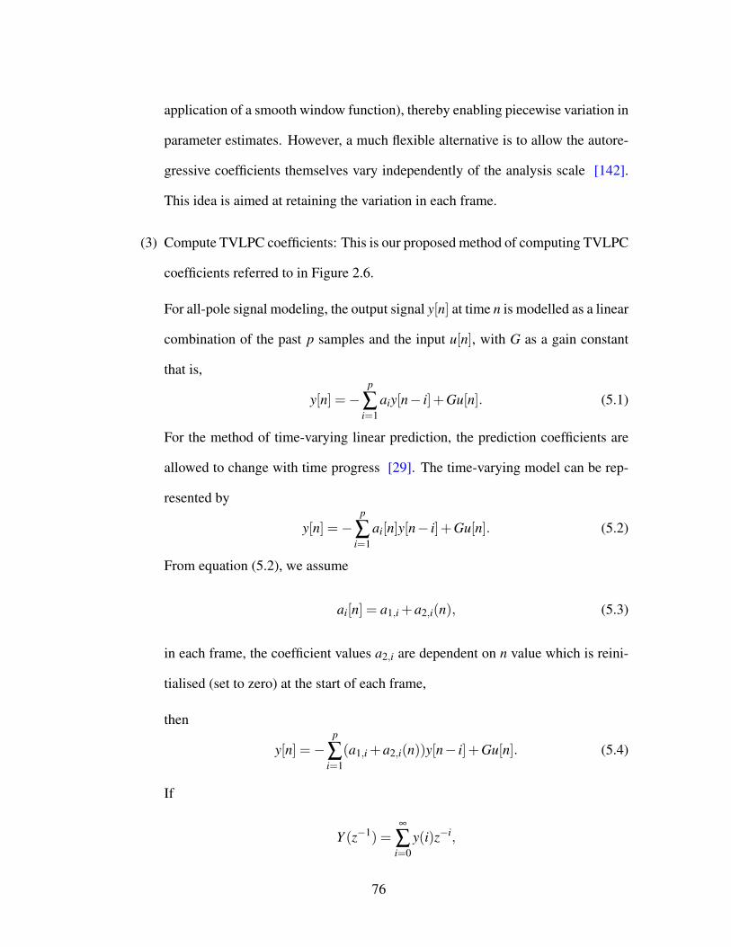
application of a smooth window function), thereby enabling piecewise variation in

parameter estimates. However, a much flexible alternative is to allow the autore-

gressive coefficients themselves vary independently of the analysis scale [142].

This idea is aimed at retaining the variation in each frame.

(3) Compute TVLPC coefficients: This is our proposed method of computing TVLPC

coefficients referred to in Figure 2.6.

For all-pole signal modeling, the output signal y[n] at time n is modelled as a linear

combination of the past p samples and the input u[n], with G as a gain constant

that is,

y[n] =−p

∑i=1

aiy[n− i]+Gu[n]. (5.1)

For the method of time-varying linear prediction, the prediction coefficients are

allowed to change with time progress [29]. The time-varying model can be rep-

resented by

y[n] =−p

∑i=1

ai[n]y[n− i]+Gu[n]. (5.2)

From equation (5.2), we assume

ai[n] = a1,i +a2,i(n), (5.3)

in each frame, the coefficient values a2,i are dependent on n value which is reini-

tialised (set to zero) at the start of each frame,

then

y[n] =−p

∑i=1

(a1,i +a2,i(n))y[n− i]+Gu[n]. (5.4)

If

Y (z−1) =∞

∑i=0

y(i)z−i,

76

U(z−1) =∞

∑i=0

u(i)z−i, and

δY (z−1)

δ z=

∞

∑i=0

y[i](−i)z−i−1; (5.5)

then Y(z−i) =−∑pi=1 a1,iz−i.Y (z−i)+∑

pi=1 a2,iz−i.δY (z−i)

δ z +

GU(z−i).

Subsequently,

(1+p

∑i=1

a1,iz−i)Y (z−1)−p

∑i=1

a2,iz−i δY (z−1)

δ z= GU(z−1). (5.6)

Let,

A1(z−1)Y (z−1)−A2(z−1)δY (z−1)

δ z= GU(z−1), (5.7)

where,

A1(z−1)Y (z−1) is the time-invariant component and −A2(z−1)δY (z−1)δ z is the time

varying component.

If the time invariant component is the dominant factor, the time invariant compo-

nent transfer function can be approximately obtained as follows,

A1(z−1)Y (z−1) = GU(z−1), (5.8)

if we assume that GU(z−1) is input and Y (z−1) is output then

H1(z−1) =1

A1(z−1). (5.9)

However, if the time varying component is the dominant factor, then the time

varying component transfer function can be approximately obtained as follows

−A2(z−1)δY (z−1)

δ z= GU(z−1), (5.10)

77

H2(z−1) =1

A2(z−1)=

(1

a2,1

)1

1+∑pi=2

a2,i+1a2,1

z−i, (5.11)

which can be represented as

H2(z−1) =b0

1+∑p−1i=1 biz−i

, (5.12)

where b0 =1

a2,1, and bi =

a2,i+1a2,1

.

In this paper, b0 represents the frame-by-frame TVLPC gain earlier introduced

and whose purpose is to determine whether our TVLPC algorithm is able to retain

the intra-frame variations.

(4) Absolute value and mel filter bank transformation: This part explains steps 4 and

5 of the proposed method. To apply mel filter transformation the signal value

must be positive. Negative values lead to a problem when modulation spectrum is

converted to logarithmic spectrum for obtaining cepstrum.

Converting from frequency to Mel scale is achieved using

mel( f ) =

1125ln(1+ f

700) if f>1kHz

f if f<1kHz,

(5.13)

where mel( f ) is the Mel-frequency scale and f is the linear frequency. The pur-

pose of the Mel-filter bank is to filter the magnitude spectrum that is passed to

it and to give an array output called Mel-spectrum. Each of the values in the

Mel-spectrum array corresponds to the result of the filtered magnitude spectrum

78

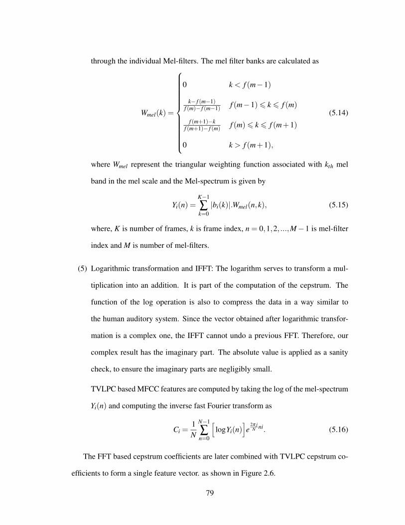
through the individual Mel-filters. The mel filter banks are calculated as

Wmel(k) =

0 k < f (m−1)

k− f (m−1)f (m)− f (m−1) f (m−1)6 k 6 f (m)

f (m+1)−kf (m+1)− f (m) f (m)6 k 6 f (m+1)

0 k > f (m+1),

(5.14)

where Wmel represent the triangular weighting function associated with kth mel

band in the mel scale and the Mel-spectrum is given by

Yi(n) =K−1

∑k=0|bi(k)|.Wmel(n,k), (5.15)

where, K is number of frames, k is frame index, n = 0,1,2, ...,M−1 is mel-filter

index and M is number of mel-filters.

(5) Logarithmic transformation and IFFT: The logarithm serves to transform a mul-

tiplication into an addition. It is part of the computation of the cepstrum. The

function of the log operation is also to compress the data in a way similar to

the human auditory system. Since the vector obtained after logarithmic transfor-

mation is a complex one, the IFFT cannot undo a previous FFT. Therefore, our

complex result has the imaginary part. The absolute value is applied as a sanity

check, to ensure the imaginary parts are negligibly small.

TVLPC based MFCC features are computed by taking the log of the mel-spectrum

Yi(n) and computing the inverse fast Fourier transform as

Ci =1N

N−1

∑n=0

[logYi(n)

]e

2π jN ni. (5.16)

The FFT based cepstrum coefficients are later combined with TVLPC cepstrum co-

efficients to form a single feature vector. as shown in Figure 2.6.

79

5.1.1 Feature enhancement

Feature enhancement techniques are applied in time series in order to enhance the fea-

tures. Additive noise components can be removed with band-pass filtering on running

spectrum domain. Running spectrum analysis (RSA) reduces more of unnecessary com-

ponents with band-pass characteristics. It is applied for the high frequency components

in the modulation spectrum domain to remove nonspeech components [115] [116]. Dy-

namic range adjustment (DRA) tends to minimize the variability of noise feature values.

In the DRA, each coefficient of a speech feature vector is adjusted proportionally to its

maximum amplitude. This in turn helps reduce noise corruption as well as preserve

important speech characteristics [111] [113] [114]. Cepstrum mean subtraction (CMS)

removes channel discrepancies in the cepstral domain by computing the sample mean

of the cepstrum vector of an utterance and then subtracting this mean from the cep-

strum vector at each frame. By cepstral mean removal, components corresponding to

the characteristics such as stationary acoustic system is removed [109] [110].

5.1.2 Model formulation

Speech feature models are formulated as follows. Five models are formulated, mod-

els 0 to 4 of feature vectors. In this study, models are formulated as follows: First,

model 0 makes use of FFT based MFCC only and is referred to as a conventional

method. Models 1 to 4 are formulated as follows: FFT based MFCC coefficients con-

sisting of 38-dimensional feature vectors are concatenated with TVLPC based MFCC

coefficients (of up to a maximum of 4 coefficients, although they can be up to a maxi-

mum of 13 cepstrum coefficients). The number of TVLPC based MFCC coefficients

appended to FFT based MFCC coefficients represents the proposed model number.

For example, appending a single TVLP-based MFCC coefficient to 38 coefficients of

80

FFT based MFCC result in model 1 and appending 2 TVLP based MFCC coefficients

to 38 coefficients of FFT-based MFCC result in model 2 and so on. Therefore, in

model 4, 4 of TVLP based MFCC coefficients are appended to the 38 cepstrum co-

efficients of model 0. The model definition is as follows: The model 0 is consid-

ered as a conventional approach (using FFT-based MFCC features only) and its 38-

parameter feature vector consisting of 12 cepstral coefficients (without the zero-order

coefficient) plus the corresponding 13 delta and 13 acceleration coefficients is given by

[b1b2 . . .b12∆b0∆b1 . . .∆b12∆2b0∆2b1 . . .∆2b12] where bi, ∆bi and ∆2bi, are MFCC, delta

MFCC and delta-delta MFCC, respectively. As for the proposed models, j( j = 1, . . . ,4)

, the intra-frame cepstrum for the time-varying coefficients [c11,c

12, . . . ,c

1j ] are appended

to the model 0 feature vector depending on the model number as follows:

• Model 0: [b1 . . .b12∆b0 . . .∆b12∆2b0 . . .∆2b12]

• Model 1: [b1 . . .b12∆b0 . . .∆b12∆2b0 . . .∆2b12][c1

1]

• Model 2: [b1 . . .b12∆b0 . . .∆b12∆2b0 . . .∆2b12][c1

1,c12]

• Model 3: [b1 . . .b12∆b0 . . .∆b12∆2b0 . . .∆2b12][c1

1, . . . ,c13]

• Model 4: [b1 . . .b12∆b0 . . .∆b12∆2b0 . . .∆2b12][c1

1, . . . ,c14].

Given that the number of time-varying LP cesptrum coefficients appended to Model 0

represents the model number, it therefore, means that model 0 has none time-varying

LP cepstrum coefficient appended to it.

5.1.3 Band-pass specifications of RSA

Running spectrum analysis (RSA) uses a bandpass. It is applied for the high frequency

components. The filter characteristics of RSA and its realization on a speech signal

81

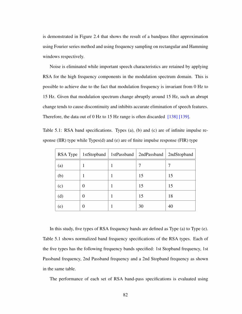
is demonstrated in Figure 2.4 that shows the result of a bandpass filter approximation

using Fourier series method and using frequency sampling on rectangular and Hamming

windows respectively.

Noise is eliminated while important speech characteristics are retained by applying

RSA for the high frequency components in the modulation spectrum domain. This is

possible to achieve due to the fact that modulation frequency is invariant from 0 Hz to

15 Hz. Given that modulation spectrum change abruptly around 15 Hz, such an abrupt

change tends to cause discontinuity and inhibits accurate elimination of speech features.

Therefore, the data out of 0 Hz to 15 Hz range is often discarded [138] [139].

Table 5.1: RSA band specifications. Types (a), (b) and (c) are of infinite impulse re-

sponse (IIR) type while Types(d) and (e) are of finite impulse response (FIR) type

RSA Type 1stStopband 1stPassband 2ndPassband 2ndStopband

(a) 1 1 7 7

(b) 1 1 15 15

(c) 0 1 15 15

(d) 0 1 15 18

(e) 0 1 30 40

In this study, five types of RSA frequency bands are defined as Type (a) to Type (e).

Table 5.1 shows normalized band frequency specifications of the RSA types. Each of

the five types has the following frequency bands specified: 1st Stopband frequency, 1st

Passband frequency, 2nd Passband frequency and a 2nd Stopband frequency as shown

in the same table.

The performance of each set of RSA band-pass specifications is evaluated using

82

Table 5.2: Average recognition accuracy (%) of elderly persons using fixed-cut-off and

gradual-cut-off frequency stop bands of 2nd order RSA pass band on clean speech and

on 15 types of noise (from NOISEX-92 database) using conventional approach at 0 dB,

5 dB, 10 dB and 20 dB SNR

RSA Clean On 15 Noises

Type speech 0 dB 5 dB 10 dB 20 dB

(a) 74.62 19.49 33.85 58.67 72.67

(b) 73.85 23.49 39.49 67.33 84.82

(c) 91.54 23.18 39.99 67.44 84.92

(d) 92.31 22.77 39.23 67.39 84.72

(e) 93.85 23.80 40.46 66.51 85.68

Table 5.3: Comparative performance in average recognition accuracy (%) of RSA

type(c) and type (e) specifications under 15 types of noise at 10 dB and 20 dB SNR

Model RSA Type(c) RSA Type(e)

10 dB 20 dB 10 dB 20 dB

Model 0 67.44 84.92 66.51 85.68

Model 1 67.08 84.77 66.51 84.61

Model 2 65.95 84.00 65.59 83.59

conventional approach both on clean speech and on the 15 types of noises at differ-

ent signal-to-noise ratios (SNRs) as shown in Table 5.2 and based on the same results,

extended experiments were conducted using RSA type (c) and type (e) on proposed ap-

proach for models 1 and 2 for validation at 10 dB and 20 dB respectively. Results of the

extended experiments shown in Table 5.3 include results for the conventional approach

83

(model 0) from Table 5.2 for performance comparison purposes. From the results, it is

observed that type (e) shows a better performance.

5.1.4 Simulation parameters and conditions of experiments

The simulation parameters shown in Table 5.4 are used in testing of the two earlier

stated speech data sets of similar pronunciation phrases, set (a): /denki/,/genki/ and

/‘tenki/ and set (b): /kyuu/,/juu/ and /chuu/ as well as the 142 Japanese common speech

phrases, designated as speech data set (d). The parameters shown in Table 5.5 are used

in testing set (c) phrases uttered by elderly persons. Initially, a database of 40 male

speakers is made available for the study. Prior to the commencement of experiments,

the initial database is split into two parts, the first part consisting of 30 speakers and is

used for the front-end feature extraction and HMM training. The second part consisting

of 10 speakers is utilised in the testing stage.

In first and second experiments, 30 male speakers each uttering 3 Japanese similar

pronunciation phrases /denki/,/genki/ and /‘tenki/ designated as set (a) and another set of

3 Japanese similar pronunciation phrases /kyuu/,/juu/ and /chuu/ both designated as set

(b) with utterance of 3 are utilized. The speech sample is 11.025 KHz and 16-bit quan-

tization. FFT based MFCC features are extracted after pre-emphasis and Hanning win-

dowing in the case of FFT based MFCC and without windowing in mel filtered TVLPC

based MFCC. In conventional approach the features are converted to 38-dimensional

feature vectors. Which features are appended with TVLPC based MFCC features. In

both feature extraction subsystems frame length and shift length are 23.2 ms (256 sam-

ples) and 11.6 ms (128 samples) respectively.

In third experiment, 30 male speakers each uttering the following 13 Japanese phrases:

(1) ohayou, (2) konnichiwa, (3) kombanwa, (4) onamaewa, (5) genki, (6) tanoshiine,

84

(7) arigato, (8) denki, (9) tenki, (10) kyuu, (11) juu, (12) migi, and (13) hidari with ut-

terance of 3 are utilised for training. Speech sample is 11.025 kHz and 16-bit quantiza-

tion. Features are extracted after pre-emphasis and Hanning windowing in the case FFT

based MFCC and without windowing in the case of mel filtered TVLPC based MFCC.

The FFT based features are later concatenated into 38-parameter feature vectors. Frame

length and shift length are 23.2 ms (256 samples) and 11.6 ms (128 samples) respec-

tively. In the proposed approach, the time invariant MFCC features are appended with

cepstrum of the dominant TVLPC based MFCC component (as explained in Eq. 5.8 and

Eq. 5.10 respectively) depending on the model number.

In the fourth experiment, 30 male speakers each uttering 142 Japanese common

speech phrases with each phrase repeated 3 times are utilized in feature extraction and

training. In testing stage, 10 speakers each uttering 142 words with each word repeated

3 times are utilized. In this experiment, the feature extraction process, concatenation

as well as training procedures are similar to the ones earlier explained. The key dif-

ference,however, is that the 142 phrases of set (d) include all other speech data set (a):

/denki/,/genki/ and /‘tenki/ , set (b): /kyuu/,/juu/ and /chuu/ and set (c) 13 speech phrases

uttered by elderly persons, being considered in this study.

/denki/,/genki/ and /‘tenki/ and set (b): /kyuu/,/juu/ and /chuu/

In these simulations the performance of conventional approach and proposed approach

are evaluated on clean speech as well as noisy speech in MATLAB (R2014a) software.

The noisy speech is evaluated on DRA, CMS/DRA, RSA and RSA/DRA. Three separate

speech databases are utilized, one with 30 speakers for the front-end feature extraction

and subsequent HMM training while the other two databases with 10 speakers (one

of elderly persons) are utilised in recognition. Independent speakers (not used in the

training) are used in HMM recognition in both proposed and conventional approach

85

Table 5.4: Parameters for 3 Similar Pronunciation phrases and 142 Japanese common

speech phrases

Parameter name Parameter value/type

Sampling 11.025 kHz (16-bit)

Frame length 23.2 ms (256 samples)

Shift length 11.6 ms (128 samples)

Pre emphasis 1−0.97z−1

Windowing Hanning window for MFCC

Feature bi(i = 1, . . . ,12), c1i (i = 1, . . . ,4),

vectors ∆bi(i = 0, . . . ,12),

∆2bi(i = 0, . . . ,12),

TVLPC order p = 14

Training set 30 male speakers,

3 utterances each

Recognition set 10 male speakers,

3 utterances each

HMM states 32

Noise 15 types from NOISEX-92

SNR 0 dB, 5 dB 10 dB, 20 dB

Noise reduction DRA, CMS/DRA,

methods RSA, RSA/DRA

experiments. In the testing stage, 0 dB, 5 dB, 10 dB and 20 dB of each of the 15

types of noises are artificially added to the original speech. In the first stage, the average

86

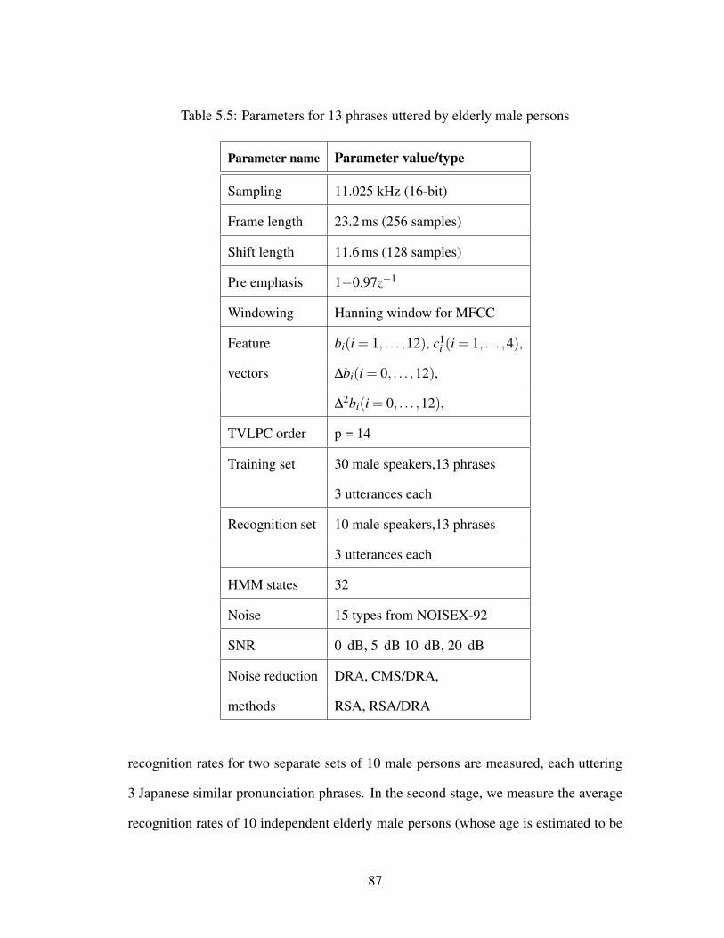
Table 5.5: Parameters for 13 phrases uttered by elderly male persons

Parameter name Parameter value/type

Sampling 11.025 kHz (16-bit)

Frame length 23.2 ms (256 samples)

Shift length 11.6 ms (128 samples)

Pre emphasis 1−0.97z−1

Windowing Hanning window for MFCC

Feature bi(i = 1, . . . ,12), c1i (i = 1, . . . ,4),

vectors ∆bi(i = 0, . . . ,12),

∆2bi(i = 0, . . . ,12),

TVLPC order p = 14

Training set 30 male speakers,13 phrases

3 utterances each

Recognition set 10 male speakers,13 phrases

3 utterances each

HMM states 32

Noise 15 types from NOISEX-92

SNR 0 dB, 5 dB 10 dB, 20 dB

Noise reduction DRA, CMS/DRA,

methods RSA, RSA/DRA

recognition rates for two separate sets of 10 male persons are measured, each uttering

3 Japanese similar pronunciation phrases. In the second stage, we measure the average

recognition rates of 10 independent elderly male persons (whose age is estimated to be

87

above 75 years), uttering 13 phrases and each phrase repeated 3 times, on 4 models at

10 dB and 20 dB as shown in Table 5.8 while in the third stage we measure the average

recognition rates of these 10 males uttering 142 Japanese common speech phrases as

shown in Table 5.9. In the fourth and last phase we measure the recognition accuracy

for the four speech data sets a) , b), c) and d) respectively, on clean speech as shown in

Table 5.10.

5.1.5 Simulation results and analysis

In this study variation of 1 % is considered to be an improvement from the conven-

tional method based on the fact that our proposed feature extraction has never been tried

before.

The simulation results are presented as follows: first, the dominant component of

TVLPC cepstrum coefficients is determined by computing the TVLPC gain frame-by-

frame on similar pronunciation phrases, second, the results for model 0 on the 15 types

of noises are shown, third, the average recognition for the 2 separate speech data sets

of the 3 similar pronunciation phrases are computed, fourth, the average recognition

accuracy on the 15 types of noise for phrases uttered by elderly persons (above the age

of 75 years ,approximately) are computed, fifth, the average recognition accuracy on the

15 types of noise for the 142 Japanese common speech phrases are computed and sixth,

the recognition accuracy for each of the four speech data sets (a), (b), (c) and (d) on

clean speech for models 0 to 4 are computed.

TVLPC gain is computed from the base 10 logarithm of absolute b0 frame-by-frame.

Given that b0 is stationary in each frame, the gain serves as the purpose of checking the

presence of variability in intra-frame coefficients. A large number of positive values

confirm the dominance of time-varying component.

88

In this study, the aim is to evaluate performance of concatenated inter-frame vari-

ation (obtained from quasi-stationary FFT based MFCC coefficients) with intra-frame

variation (obtained from TVLPC based MFCC). Observing the dominance of b0 helps

in confirming the presence of intra-frame variation.

It is also used as a benchmark in determining whether Equation (5.8) or (5.10) should

be used in obtaining features in the proposed method.

The 15 types of noises used in the experiments are based on Signal Processing In-

formation Base (SPIB) noise data measured in field by Speech Research Unit (SRU) at

Institute for Perception-TNO, Netherlands, United Kingdom, under the project number

2589-SAM (Feb. 1990) [79] [143].

Experiments for 142 Japanese common speech phrases on models 0 and 1 are con-

ducted on the 15 types of noises with CMS/DRA and RSA to show how the recognition

performance varies depending on the noise levels. The performance of each noise type

are different as shown in Table 5.11 depending on the noise levels. In signal processing,

white noise is a random signal having equal intensity at different frequencies, giving it

a constant power. Babble noise is noise encountered when a crowd or a group of people

are talking together and is considered as one of the best noises for masking speech. As

such, the effectiveness of the proposed method can be evaluated based on the perfor-

mance of white and babble noises. Therefore, the observed increase in recognition rate

under these two noises demonstrates that the method is effective especially for noisy

conditions.

5.1.5.1 Simulation results of TVLPC gain

The simulations are based on speech analysed using mel filtered TVLPC of an auto-

regressive model with pre-emphasis but without windowing. A speech segment, 128

89

Figure 5.1: Waveform for 7 frames of a Japanese phrase /genki/ after VAD and pre-

emphasis and magnitude spectrum of normalized TVLPC coefficients frame-by-frame.

Figure 5.2: Waveform for 7 frames of a Japanese phrase /denki/ after VAD and pre-

emphasis and magnitude spectrum of normalized TVLPC coefficients frame-by-frame.

samples (11.6ms) per frame of 7 frames, is extracted from the speech signal of each

phrase, post voice activity detection (VAD) using short term energy (STE) respectively.

The VAD process eliminates silent parts. The time-varying LPC gain for each frame in

the speech segment is then computed.

Figures 5.1, 5.2, and 5.3, show the waveforms and their corresponding time-varying

LPC gain for three Japanese phrases; /genki/, /denki/ and /tenki/. The top graph in

Figure 5.1 shows a waveform for “genki” while shown immediately below is the frame-

90

Figure 5.3: Waveform for 7 frames of a Japanese phrase /tenki/ after VAD and pre-

emphasis and magnitude spectrum of normalized TVLPC coefficients frame-by-frame.

Table 5.6: Average recognition accuracy (%) for similar pronunciation phrases /genki/,

/denki/ and /tenki/ on 15 types of noise at 10 dB and 20 dB SNR

Models DRA CMS/DRA RSA RSA/DRA

10 dB 20 dB 10 dB 20 dB 10 dB 20 dB 10 dB 20 dB

Model 0 55.56 67.78 58.00 74.00 61.33 71.56 52.89 66.00

Model 1 56.45 70.67 58.00 73.33 61.78 71.56 54.67 67.11

Model 2 56.22 70.45 56.67 71.55 62.64 70.67 52.89 66.44

Model 3 58.45 68.67 58.44 73.56 60.89 70.67 53.33 66.44

Model 4 56.00 72.00 55.78 71.78 58.67 67.11 51.55 64.12

by-frame TVLPC gain graph. Figure 5.2 and Figure 5.3 show the comparative results for

/denki/ and /tenki/ in the same order respectively. In all three phrases, the TVLPC gains

are mostly positive values. This confirms that the time-varying component is dominant.

We can therefore be certain that our algorithm is able to retain the time variation in

most of the speech frames and therefore coefficients obtained can be considered in our

experiments.

91

Table 5.7: Average recognition accuracy (%) for similar pronunciation phrases /kyu/,

/juu/ and /chuu/ on 15 types of noise at 10 dB and 20 dB SNR

Models CMS/DRA RSA

10 dB 20 dB 10 dB 20 dB

Model 0 57.78 70.89 57.33 70.44

Model 1 57.56 71.56 58.44 69.78

Table 5.8: Average recognition accuracy (%) of 13 phrases for elderly male persons on

15 types of noise at 10 dB and 20 dB SNR

Models DRA CMS/DRA RSA RSA/DRA

10 dB 20 dB 10 dB 20 dB 10 dB 20 dB 10 dB 20 dB

Model 0 57.38 76.75 67.33 76.31 67.44 84.92 61.51 69.59

Model 1 57.54 77.18 67.74 76.41 67.08 84.77 61.23 69.64

Model 2 56.68 76.82 67.59 75.79 65.95 84.00 60.97 69.03

Model 3 55.79 76.46 67.44 76.20 66.00 83.64 61.08 68.87

Model 4 56.56 76.98 67.38 76.20 66.41 83.64 61.13 68.87

Table 5.9: Average recognition accuracy (%) for 142 Japanese common speech phrases

on 15 types of noise at 10 dB and 20 dB SNR

Models CMS/DRA RSA

10 dB 20 dB 10 dB 20 dB

Model 0 72.16 87.77 69.75 85.65

Model 1 72.03 87.86 69.58 86.15

92

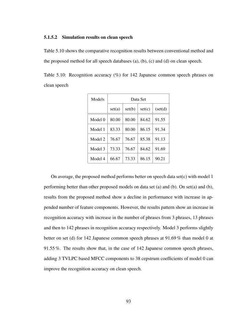
5.1.5.2 Simulation results on clean speech

Table 5.10 shows the comparative recognition results between conventional method and

the proposed method for all speech databases (a), (b), (c) and (d) on clean speech.

Table 5.10: Recognition accuracy (%) for 142 Japanese common speech phrases on

clean speech

Models Data Set

set(a) set(b) set(c) (set(d)

Model 0 80.00 80.00 84.62 91.55

Model 1 83.33 80.00 86.15 91.34

Model 2 76.67 76.67 85.38 91.13

Model 3 73.33 76.67 84.62 91.69

Model 4 66.67 73.33 86.15 90.21

On average, the proposed method performs better on speech data set(c) with model 1

performing better than other proposed models on data set (a) and (b). On set(a) and (b),

results from the proposed method show a decline in performance with increase in ap-

pended number of feature components. However, the results pattern show an increase in

recognition accuracy with increase in the number of phrases from 3 phrases, 13 phrases

and then to 142 phrases in recognition accuracy respectively. Model 3 performs slightly

better on set (d) for 142 Japanese common speech phrases at 91.69 % than model 0 at

91.55 %. The results show that, in the case of 142 Japanese common speech phrases,

adding 3 TVLPC based MFCC components to 38 cepstrum coefficients of model 0 can

improve the recognition accuracy on clean speech.

93

Table 5.11: Recognition performance accuracy (%) of the 15 types of noises on 142

Japanese common speech phrases using conventional approach (model 0) at 10 dB and

20 dB SNR of CMS/DRA and RSA

Noise type CMS/DRA RSA

10 dB 20 dB 10 dB 20 dB

White 62.75 82.68 51.20 80.49

Pink 69.79 88.45 59.01 84.79

HF 75.85 88.10 67.96 85.56

Babble 72.46 89.44 78.10 87.68

Factory 1 62.25 86.06 67.32 86.06

Factory 2 84.23 90.77 82.89 88.80

Cockpit 1 68.66 89.08 62.25 86.55

Cockpit 2 61.83 84.15 54.01 83.10

DestroEg 83.31 90.49 72.75 86.76

DestrOps 58.87 85.35 75.28 86.69

F-16 80.14 90.00 74.01 86.83

Leopard 88.87 91.83 86.90 88.94

M109 80.56 90.63 81.48 88.31

Machine gun 52.18 77.75 50.70 75.21

Volvo 340 80.63 91.83 82.46 89.01

5.1.5.3 Simulation results for 10 speakers and 3 similar phrases (set A)

Simulations were conducted on 3 similar pronunciation phrases /genki/, /denki/ and

/tenki/ for models 0 to 4 using 15 types of noise from NOISEX-92 database [143]. The

results shown in Table 5.6 indicate that model 3 performs better at 58.45% at 10 dB

94

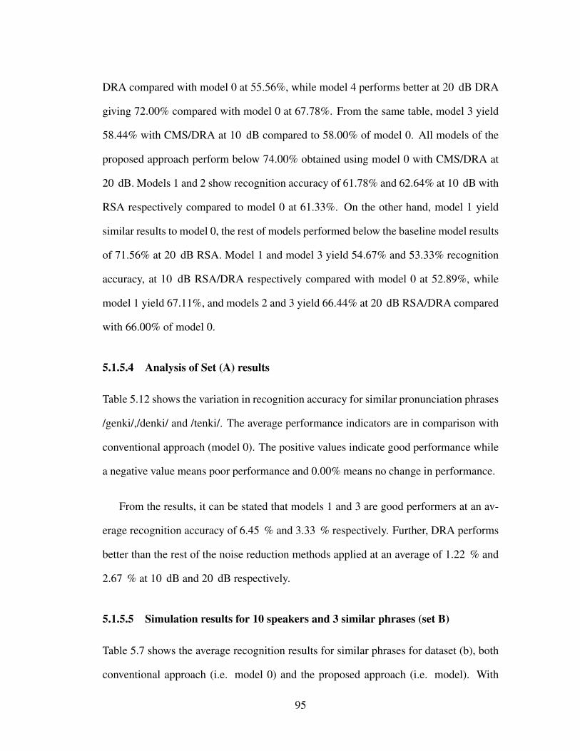
DRA compared with model 0 at 55.56%, while model 4 performs better at 20 dB DRA

giving 72.00% compared with model 0 at 67.78%. From the same table, model 3 yield

58.44% with CMS/DRA at 10 dB compared to 58.00% of model 0. All models of the

proposed approach perform below 74.00% obtained using model 0 with CMS/DRA at

20 dB. Models 1 and 2 show recognition accuracy of 61.78% and 62.64% at 10 dB with

RSA respectively compared to model 0 at 61.33%. On the other hand, model 1 yield

similar results to model 0, the rest of models performed below the baseline model results

of 71.56% at 20 dB RSA. Model 1 and model 3 yield 54.67% and 53.33% recognition

accuracy, at 10 dB RSA/DRA respectively compared with model 0 at 52.89%, while

model 1 yield 67.11%, and models 2 and 3 yield 66.44% at 20 dB RSA/DRA compared

with 66.00% of model 0.

5.1.5.4 Analysis of Set (A) results

Table 5.12 shows the variation in recognition accuracy for similar pronunciation phrases

/genki/,/denki/ and /tenki/. The average performance indicators are in comparison with

conventional approach (model 0). The positive values indicate good performance while

a negative value means poor performance and 0.00% means no change in performance.

From the results, it can be stated that models 1 and 3 are good performers at an av-

erage recognition accuracy of 6.45 % and 3.33 % respectively. Further, DRA performs

better than the rest of the noise reduction methods applied at an average of 1.22 % and

2.67 % at 10 dB and 20 dB respectively.

5.1.5.5 Simulation results for 10 speakers and 3 similar phrases (set B)

Table 5.7 shows the average recognition results for similar phrases for dataset (b), both

conventional approach (i.e. model 0) and the proposed approach (i.e. model). With

95

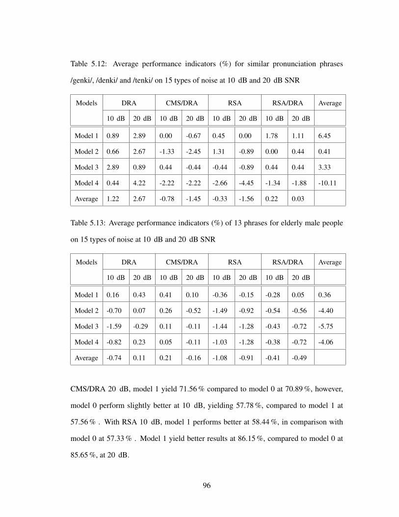
Table 5.12: Average performance indicators (%) for similar pronunciation phrases

/genki/, /denki/ and /tenki/ on 15 types of noise at 10 dB and 20 dB SNR

Models DRA CMS/DRA RSA RSA/DRA Average

10 dB 20 dB 10 dB 20 dB 10 dB 20 dB 10 dB 20 dB

Model 1 0.89 2.89 0.00 -0.67 0.45 0.00 1.78 1.11 6.45

Model 2 0.66 2.67 -1.33 -2.45 1.31 -0.89 0.00 0.44 0.41

Model 3 2.89 0.89 0.44 -0.44 -0.44 -0.89 0.44 0.44 3.33

Model 4 0.44 4.22 -2.22 -2.22 -2.66 -4.45 -1.34 -1.88 -10.11

Average 1.22 2.67 -0.78 -1.45 -0.33 -1.56 0.22 0.03

Table 5.13: Average performance indicators (%) of 13 phrases for elderly male people

on 15 types of noise at 10 dB and 20 dB SNR

Models DRA CMS/DRA RSA RSA/DRA Average

10 dB 20 dB 10 dB 20 dB 10 dB 20 dB 10 dB 20 dB

Model 1 0.16 0.43 0.41 0.10 -0.36 -0.15 -0.28 0.05 0.36

Model 2 -0.70 0.07 0.26 -0.52 -1.49 -0.92 -0.54 -0.56 -4.40

Model 3 -1.59 -0.29 0.11 -0.11 -1.44 -1.28 -0.43 -0.72 -5.75

Model 4 -0.82 0.23 0.05 -0.11 -1.03 -1.28 -0.38 -0.72 -4.06

Average -0.74 0.11 0.21 -0.16 -1.08 -0.91 -0.41 -0.49

CMS/DRA 20 dB, model 1 yield 71.56 % compared to model 0 at 70.89 %, however,

model 0 perform slightly better at 10 dB, yielding 57.78 %, compared to model 1 at

57.56 % . With RSA 10 dB, model 1 performs better at 58.44 %, in comparison with

model 0 at 57.33 % . Model 1 yield better results at 86.15 %, compared to model 0 at

85.65 %, at 20 dB.

96

Table 5.14: Average performance indicators (%) for similar pronunciation phrases /kyu/,

/juu/ and /chuu/ on 15 types of noise at 10 dB and 20 dB SNR

Models CMS/DRA RSA Average

10 dB 20 dB 10 dB 20 dB

Model 1 -0.22 0.67 1.11 -0.66 0.90

5.1.5.6 Analysis of Set (B) results

Table 5.14 shows the performance variation in recognition accuracy for similar pro-

nunciation phrases /kyu/, /juu/ and /chyu/ in comparison to the conventional approach

(model 0). From the results it has been shown that model 1 is slightly better at average

of 0.90 %. It must be pointed out that the indicator is lower than the one shown in Table

5.12 considering that it is based on 4 noise levels and not 8 noise levels as the case is in

Table 5.12.

5.1.5.7 Simulation results for 10 speakers and 13 phrases uttered by elderly per-

sons

Table 5.8 shows the average recognition results for elderly persons for both conventional

approach (i.e. model 0) and the proposed approach (i.e. models 1 to 4). With DRA at

both 10 dB, and 20 dB, model 1 at 57.54 %, and 77.18 %, is better compared to model

0 at 57.38 %, and 67.33 %, respectively. With CMS/DRA at 10 dB, and 20 dB, model 1

is better at 67.74 % and 76.41 % compared to model 0 at 67.33 %, 76.31 % respectively.

With RSA at 10 dB, and 20 dB, model 0 performs better at 67.44 %, and 84.92 %

with the closest model in performance being model 1 at 67.08 %, and 84.77 %, respec-

tively.Regarding RSA/DRA at 10 dB, models 0 yield 61.51 %, followed by model 1 at

97

61.23 %. As for RSA at 20 dB, model 1 performs slightly better at 69.64 %, followed

by model 0 at 69.59 %,.

5.1.5.8 Analysis of results for 13 phrases

Table 5.13 shows the performance variation in recognition accuracy for 13 phrases of

elderly male people in comparison to the conventional approach (model 0).

Table 5.15: Average performance indicators (%) for 142 Japanese common speech

phrases on 15 types of noise at 10 dB and 20 dB SNR

Models CMS/DRA RSA Average

10 dB 20 dB 10 dB 20 dB

Model 1 -0.13 0.09 -0.17 0.50 0.29

The results show that model 1 is a good performer with an overall average of 0.36

%. CMS/DRA improves the results by an average of 0.21 % at 10 dB followed those of

DRA with 0.11 % at 20 dB.

5.1.5.9 Simulation results for 10 speakers and 142 Japanese common speech phrases

Table 5.9 shows the average recognition results for 142 Japanese common speech phrases.

The proposed method performs slightly better than conventional method on CMS/DRA

and RSA 20 dB with 87.86 % and 86.15 % compared to 87.77 % and 85.65 % respec-

tively.

In the case of similar pronunciation phrases, the proposed approach show positive

results on ’genki”, “tenki” and “denki” with CMS/DRA. while slight improvements are

achieved on “kyu”, “juu” and “chuu”, with CMS/DRA at 20 dB and RSA at 10 dB.

98

Overall performance of the proposed approach shows improvement on 142 Japanese

common speech phrases.

5.1.5.10 Analysis of results for 142 Japanese common speech phrases

Table 5.15 shows the performance variation in recognition accuracy in comparison to the

conventional approach (model 0). The results show that model 1 improves the results

by 0.29 %.

5.1.6 Discussion

In this chapter findings of the experiments are discussed and a comparatison is made

with other reported methods. The effects of TVLPC coefficients on speech recogntion

is also showm.

The proposed method was adapted to demonstrate the plausibility of concatenating

time invariant and time varying speech features in speech recognition. This was thought

to be effective considering that multiple acoustic features of speech signal have been

investigated elsewhere and have shown that the accuracy of automatic speech recogni-

tion systems can be improved by the combination of different acoustic features [144].

However, unlike in other reported works, not the entire TVLPC cepstrum coefficients

are utilized. Instead cepstrum components are added incrementally , model-by-model,

in each of the proposed model.

In the study, recognition accuracies are calculated for various cases (4 sets of data,

models, and noises types). They have been shown in tables and compared.

Table 6 shows that recognition accuracy increases with the number of reference

speech waveforms (utterances) available for the reference words. The increase in recog-

nition accuracy rates with increase in words used for training is as reported by other

99

researcher elsewhere [145]. In addition, just generically increasing the vocabulary size

can improve the accuracy for many common speech words but degrades the recognition

rate for less common speech words [146].

Table 5.12 shows model 1 performing well at 6.45 % and with DRA being the best

performer among all noise reduction methods while model 4 performing poorly at -

10.11 %. Model 4 results seem to suggest that increasing the number intra-frame cep-

strum coefficients can result in poor performance particularly when RSA and DRA are

combined.

The experiments have also shown the effect of adding TVLPC coefficients for speech

recognition in adverse conditions. Table 5.13 shows model 1 to be a good performer at

an average of 0.36 %. Equally, Table 5.14 shows model 1 to have a slight improvement

in recognition with RSA at 10 dB giving a performance improvement of 1.11 % and an

overall improvement of 0.90 % while Table 5.15 shows model 1 being a good performer

at 0.29 %. From these results, it has been shown that TVLPC coefficients are good at

capturing transistions in plosive phrases /genki/, /denki/ and /tenki/ than on /kyu/, /juu/

and /chuu/. Depending on the pronunciation context and the frequency of such words

also affects the accuracy of the system [147]. Therefore, it can stated confidently that

the proposed method performs better with models 1 and 3.

Since TVLPC coefficients are good at capturing transition features, it is naturally

expected that they may have positive effects for recognition for phonemes with non-

stationary features. They can still work for noisy conditions by decomposing the noisy

signal into spectral components by means of a spectral transform, a filter bank or loga-

rithmic transform [148].

RSA and DRA are thought to be effective for noisy speech. However, results of a

combination of both does not give a good match with expectations. The possible cause

100

of such low accuracy may be due to the distortion of the speech waveform after noise

reduction. RSA reduces more of unnecessary components with band-pass characteris-

tics. As the general dismal performance of the proposed method, it is plausible that the

discontinuity at concatenation joints of acoustic units may be the cause, which suggests

need for smoothing techniques [149].

5.1.7 Summary

Currently, MFCC and TVLPC are separately used for speech feature extraction with ac-

ceptable performance. However, our findings demonstrate that a combination of MFCC

and TVLPC shows better performance with model 1 and 3 showing improved recogni-

tion results when compared to the conventional and other proposed models.

Models 1 and 3 give an average improvement of 6.45% and 3.33% to the conven-

tional method.

Although models 1 and 3 will require further optimization, our study results suggest

that the two models could be used in the front-end feature extraction process in ASR

systems.

5.2 Noise suppression in modulation spectrum

Speech recognition systems often suffer from various sources of variability due to cor-

rupted speech signal faetures. Techniques aimed at both reducing noise corruption as

well as preserving important speech characteristics are often required. This section

focuses on the use offlexible band-pass RSA FIR filtering scheme in a modulation spec-

trum domain. Several ASR systems that make use of RSA for noise suppression in con-

tinuous speech recognition [150] have been developed before and work successfully. In

101

the authors’ view, the use of RSA for isolated speech phrases has yet to be elucidated.

In addition, the use of effectiveness of higher frequency components of RSA on recog-

nition of isolated word remains unknown. In this paper, the use of MFCC [31] [32]

with RSA for noise suppression for isolated word recognition is being proposed.

5.2.1 Feature extraction method

Although removing low-frequency components with a high-pass RSF filter can reduce

the noise, the speech spectrum covers a wider frequency range. There is low energy of

noise in the high-frequency band. Therefore, it is anticipated that incorporating high-

frequency components in HMM training would improve recognition accuracy. Unlike

RSF which increases the calculation cost by its order number, proposed wide band-pass

RSA is simple and computationally effective. RSF is fixed based on the order number

while RSA band-pass can be adapted based on noise level as demonstrated later.

Based on the above, the following way for robust speech recognition can be pro-

posed;

(i) Evaluate SNR at 5 levels of 5 dB, 10 dB, 15 dB, 20 dB, 25 dB, and ∞ respec-

tively.

(ii) According to SNR, the specification of RSA should be incrementally changed in

creating different sets of filter banks to include higher order frequency compo-

nents.

(iii) for (ii), several intra filter bank specifications of RSA should be given and be

evaluated.

102

5.2.2 Signal Analysis

Now the feature extraction method used in the proposed phrase speech recognition sys-

tem is presented. Shown in Figure 5.4 are the steps involved in obtaining speech features

using the conventional approach. In the initial step of the feature extraction, we conduct

a pre-emphasis of the sampled speech signal. Every 11.6ms, a Hanning window is ap-

plied to pre-emphasized 23.2ms long speech segments. Later the short-term spectrum

by Fast Fourier Transform (FFT) is computed. Thereafter, the outputs of 40 overlapping

Mel scale triangular filters are computed. For each filter, the output is a sum of weighted

spectral magnitudes. Then a linear transformation is performed on the first 13 filters and

logarithmic transformation on the 27 filter bank outputs followed by Discrete Cosine

Transform which outputs 13 cepstrum coefficients. Since the human auditory system is

sensitive to time evolution of the spectral content of speech signal, an attempt is made

to include the extraction of delta and delta-delta of static features as part of feature anal-

ysis. Lastly these dynamic coefficients with the static coefficients are concatenated to

make up the final output of feature analysis representation.

The details of FFT based MFCCs and its computation are discussed in [140] [141]

and explained as follows:

(1) Pre-emphasis: When a digitized speech signal, s(n), is passed through a first-order

finite impulse response (FIR) filter, it is put into spectrally flatten signal and made

less susceptible to finite precision effects later in the signal processing. The fixed

first-order system is

H(z) = 1−0.97z−1 (5.17)

(2) Windowing: Speech is a non-stationary signal where properties change quite

rapidly over time. It is preferable to have smooth joins between sections and

103

Figure 5.4: MFCC: Complete pipeline for feature extraction

that is the function of the window. The frame step is usually something like 1/2

or a 1/3 of total samples, which allows some overlap to the frames. The next step

in the processing is to window each individual frame. If we define the window as

w(n), 0 6 n 6 N−1, then the result of Hanning window, has the form

w(n) = 0.5(1− cos(2nπ

N−1)) = hav(

2nπ

N−1), (5.18)

sw(n) = s′(n)w(n), (5.19)

where, sw(n) is the signal after windowing and s′(n) is pre-emphasized speech

signal.

(3) Spectral analysis by fast Fourier transform (FFT): To convert each frame of N

samples from time domain into frequency domain FFT is used. The spectrum is

calculated by using discrete Fourier transform (DFT) at discrete windowed signal

sw(n) that is achieved by time sampling of a continuous signal s(n). In this case,

104

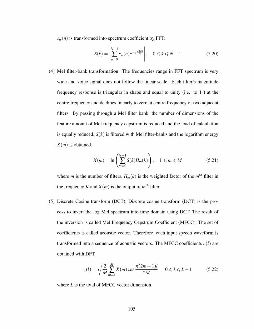
sw(n) is transformed into spectrum coefficient by FFT:

S(k) =

∣∣∣∣∣N−1

∑n=0

sw(n)e− j 2πknN

∣∣∣∣∣ , 0 6 k 6 N−1 (5.20)

(4) Mel filter-bank transformation: The frequencies range in FFT spectrum is very

wide and voice signal does not follow the linear scale. Each filter’s magnitude

frequency response is triangular in shape and equal to unity (i.e. to 1 ) at the

centre frequency and declines linearly to zero at centre frequency of two adjacent

filters. By passing through a Mel filter bank, the number of dimensions of the

feature amount of Mel frequency cepstrum is reduced and the load of calculation

is equally reduced. S(k) is filtered with Mel filter-banks and the logarithm energy

X(m) is obtained.

X(m) = ln

(N−1

∑m=0

S(k)Hm(k)

), 1 6 m 6 M (5.21)

where m is the number of filters, Hm(k) is the weighted factor of the mth filter in

the frequency K and X(m) is the output of mth filter.

(5) Discrete Cosine transform (DCT): Discrete cosine transform (DCT) is the pro-

cess to invert the log Mel spectrum into time domain using DCT. The result of

the inversion is called Mel Frequency Cepstrum Coefficient (MFCC). The set of

coefficients is called acoustic vector. Therefore, each input speech waveform is

transformed into a sequence of acoustic vectors. The MFCC coefficients c(l) are

obtained with DFT.

c(l) =

√2M

M

∑m=1

X(m)cosπ(2m+1)l

2M, 0 6 l 6 L−1 (5.22)

where L is the total of MFCC vector dimension.

105

5.2.3 Band-pass specifications of RSA

In continuous speech recognition RSA is applied for the high frequency component us-

ing a band-pass of finite impulse response (FIR) type. The technique helps to eliminate

noise while retaining important speech characteristics in the modulation spectrum do-

main as reported in [138] [139]. RSA has been applied for the frequency components

of between 1 Hz and 15 Hz in the modulation spectrum domain. The data out of 1 Hz

to 15 Hz range is often discarded. In addition to its use for continuous speech recogni-

tion, its merits for the phrase recognition have been found through several evaluations

of its filter banks specifications. In this way, all available frequency components in the

modulation spectrum domain, except for the one below 1 Hz, are utilised in determining

the most robust filter banks. By judicious choices, the following band-pass ranges are

selected for evaluation; 1 Hz to 7 Hz, 1 Hz to 15 Hz, 1 Hz to 30 Hz, 1 Hz to 35 Hz

and 1 Hz to 40 Hz and each band-pass is evaluated respectively. Table 5.16 shows five

types of RSA frequencies band-pass specifications which we have defined as Type (a)

to Type (e). For the purpose of this study, Type (a) is designated as a wide bandwidth

specification, Type (b) (c), (d) and (e) as narrow bandwidths. Like in conventional FIR

filter, each of the bandwidth is designed to have a 1st stop band frequency, a 1st pass

band frequency, a 2nd pass band frequency and a 2nd stop band frequency respectively.

The range between the 1st pass band frequency and the 2nd pass band frequency repre-

sents the number of frequency components to be considered in the respective bandwidth

specification. Subsequently, Type (a) has 7 frequency components, Type (b) has 15 fre-

quency components, Type (c) has 30 frequency components, Type (d) has 35 frequency

components, while Type (e) has 40 frequency components, respectively. Table 5.17

shows the sub bandwidths specifications within the narrow bandwidths between Types

(c) and (d) and between Types (d) and (e). It is aimed to determine the tendency in the

106

relative improvement of RSA over RSF. Therefore, for the purpose of this study, Types

(c1) and (c2) are sub bandwidths between Types (c) and (d) while Types (d1) and (d2)

are sub bandwidths between Types (c) and (d), respectively. Type(c1) has 32 frequency

components, Type(c2) has 34 frequency components, Type(d1) has 36 frequency com-

ponents while Type(d2) has 38 frequency components. The implementation is as shown

in Figure 5.5.

Table 5.16: RSA band specifications. Type (a) is wide bandwidth, Types (b), (c), (d)

and (e) are of narrow bandwidths (FIR) type

RSA Type 1stStopband 1stband-pass 2ndband-pass 2ndStopband

(a) 1 1 7 7

(b) 1 1 15 15

(c) 1 1 30 30

(d) 1 1 35 35

(e) 1 1 40 40

5.2.4 Simulation parameters and conditions of experiments

The main method used for speech enhancement is filtering. The performance of high-

pass RSF IIR filtering with several band-pass RSA FIR filtering banks are compared.

The simulation parameters shown in Table 5.18 are used in testing of the isolated Japanese

common speech phrases. In our experiments, an initial database of 40 male speakers is

made available for the study. Prior to the commencement of experiments, the database

is split into two sets, the first set consisting of 30 speakers, each speaker uttering 100

Japanese common speech phrases, and each phrase repeated 3 times, is used for the

107

Table 5.17: RSA sub band specifications for wide band-pass. Type (c1) and (c2) are sub

band-pass for Type (c). Type (d1) and Type (d2) are sub band specifications for Type

(d) wide band-pass

RSA Type 1stStopband 1stband-pass 2ndband-pass 2ndStopband

(c1) 1 1 32 32

(c2) 1 1 34 34

(d1) 1 1 36 36

(d2) 1 1 38 38

Figure 5.5: Implementation of band-pass RSA FIR filter banks for noise suppression

front-end feature extraction and HMM training. The second set consisting of 10 speak-

ers (classified as independent speakers), each speaker uttering 100 phrases and each

phrase repeated once is utilised in the testing stage. The speech sample is 11.025 KHz

and 16-bit quantization. FFT based MFCC features are extracted after pre-emphasis and

Hanning windowing.

108

Table 5.18: The condition of speech recognition experiments

Parameter name Parameter value/type

Recognition Task Isolated 100 phrases

Speech database (a) 100 Japanese common speech phrases

Sampling 11.025 kHz (16-bit)

Frame length 23.2 ms (256 samples)

Shift length 11.6 ms (128 samples)

Pre emphasis 1−0.97z−1

Windowing Hanning window

Speech bi(i = 1, . . . ,12)

Feature ∆bi(i = 0, . . . ,12),

vectors ∆2bi(i = 0, . . . ,12),

Training Set 30 male speakers,

100 phrases ,

3 utterances each

Tested Set 10 male speakers,

100 isolated phrases

1 utterance each

Acoustic Model 32-states isolated word HMMs

Noise 15 types from NOISEX-92

varieties heightSNR 5 dB 10 dB, 15 dB, 20 dB 25 dB,

Filtering RSF, RSA,

methods

109

In the simulations, the performance of conventional approach are evaluated under

noisy and clean conditions in MATLAB (R2014a) software. In both conditions, high-

pass RSF IIR filtering scheme and 9 RSA FIR filters (2 wide bands, and 7 narrow bands)

are evaluated. An isolated speech databases of Japanese common speech phrases is

utilized. Independent speakers (not used in the training) are used in HMM recognition

in the experiments. In the testing stage, 5 dB, 10 dB, 15 dB, 20 dB and 25 dB of

the 15 types of noises are artificially added to the original speech. In the first stage,

the average recognition rates for 10 speakers is measured, each uttering 100 Japanese

common speech phrases on RSF and 9 RSA bandwidth specifications for Type (a) to

Type (e) at 5 dB and 10 dB 15 dB, 20 dB and 25 dB SNR as shown in Table 5.19. Table

5.21 shows a summary of the average recognition accuracy for the purpose of critical

comparison while Table 5.22 shows the relative improvement in recognition accuracy

as performance indicators of individual RSA band-pass specifications compared with a

high-pass RSF IIR filtering on Japanese common speech phrases database.

5.2.5 Simulation results and analysis

The signal-to-noise ratio (SNR) of a system is the ratio of the average signal level to

the average noise level at the output, where the noise is any unwanted signal added to

the input by the system or from the environment. The influence of 15 noises on various

acoustic characteristics of speech utterances is described below. In each experiment sim-

ulation, an average recognition rate is used to determine whether RSA performed better

than RSF on 5 kinds of noise levels. Analyses are carried out for the speech database.

The analysis use RSF and RSA filters and 5 noise levels (at 5 dB, 10 dB, 15 dB, 20 dB

and 25 dB) as independent variables. The presentation of results focuses on the perfor-

mance of RSA on the various acoustic measures. The simulation results are presented

110

as follows: first, we show the signal-noise-ratio (SNR) results for RSF and RSA for the

15 types of noises on Japanese common speech phrases, then we provide a summary

for the average recognition accuracy under the 15 noises and on clean speech. We then

compute the relative improvement in recognition accuracy as performance indicators.

The 15 types of noises used in the experiments are based on Signal Processing In-

formation Base (SPIB) noise data measured in field by Speech Research Unit (SRU) at

Institute for Perception-TNO, Netherlands, United Kingdom, under the project number

2589-SAM (Feb. 1990) [79] [143].

In this paper the model formulation is as follows: The model uses FFT based MFCC

coefficients consists of 38-dimensional feature vectors. The 38-parameter feature vector

consisting of 12 cepstral coefficients (without the zero-order coefficient) plus the corre-

sponding 13 delta and 13 acceleration coefficients is given by

[b1b2 . . .b12∆b0∆b1 . . .∆b12∆2b0∆2b1 . . .∆2b12] where bi, ∆bi and ∆2bi, are MFCC, delta

MFCC and delta-delta MFCC, respectively.

The recognition accuracy was evaluated by the average of the 10 independent male

speakers. It can be observed from Table 5.19 results that each type of noise has its

special effects on the speech signal. In addition, the signal-to-noise rations (SNRs) for

various noisy environments can result in different recognition accuracies depending on

the type of filter as well as on the number of frequency components in the case of RSA.

Table 5.21 is a summary of the recognition accuracies ON 15 types of noises at 5

dB, 10 dB, 15 dB, 20 dB and 25 dB . The increasing tendency in recognition accuracy

from 5 dB to 25 dB is as expected. All RSA Types exhibited ’normal’ increase in results

from large to small SNRs. RSA Type(d) showed better results than the rest. Among the

five noise levels, at 54.04 %, 5 dB was the best. This signifies that the approach is much

more effective for large noise than it is for less noisy conditions. Table 5.22 shows the

111

Table 5.19: Average recognition accuracy (%) for 100 words Japanese common speech

phrases on 15 types of noise at 5 dB, 10 dB, 15 dB ,20 dB , and 25 dB SNR

Models RSF RSA Type(a) RSA Type(b)

5 dB 10 dB 15 dB 20 dB 25 dB 5 dB 10 dB 15 dB 20 dB 25 dB 5 dB 10 dB 15 dB 20 dB 25 dB

white 33.20 66.00 84.30 92.30 95.50 27.80 59.40 79.40 87.90 90.90 35.30 66.80 82.80 91.00 93.10

pink 1 28.90 74.00 91.30 94.90 96.90 27.90 68.30 85.50 90.30 91.90 32.10 74.50 89.10 93.40 94.10

hfchannel 36.60 74.10 89.00 94.90 96.90 36.40 73.20 87.00 91.10 92.30 45.50 79.70 90.30 93.80 95.00

babble 47.20 85.50 94.40 96.90 97.20 51.70 84.10 91.00 92.20 92.80 59.90 90.00 94.30 95.30 95.40

factory1 33.20 78.40 90.90 95.70 97.20 36.70 77.10 88.50 92.20 92.60 41.70 81.50 90.80 94.30 95.20

factory2 51.80 91.70 97.30 97.30 97.40 56.10 89.70 93.20 93.30 93.20 66.10 93.10 95.00 95.20 95.50

buccaneer1 29.60 71.80 91.20 95.60 97.30 28.70 69.20 86.80 91.00 93.00 30.80 73.50 90.80 94.40 95.20

buccaneer2 33.20 68.80 85.50 93.10 96.00 30.00 63.90 80.70 88.40 91.80 34.70 69.40 85.70 91.60 94.20

destroterengine 50.40 86.30 94.80 96.90 97.10 47.20 82.50 89.40 92.40 92.90 52.90 85.50 92.60 94.80 95.20

destroyerops 48.40 86.40 94.60 96.10 97.10 50.20 84.10 90.40 92.10 92.60 50.40 84.90 92.80 94.70 95.40

f16 43.80 86.30 94.50 96.90 97.10 40.80 82.10 90.80 92.80 92.70 48.10 86.90 93.10 95.20 95.30

leopard 74.10 96.50 97.40 97.40 97.50 79.00 92.60 93.20 93.20 93.00 85.00 94.80 95.50 95.60 95.80

m109 50.40 90.00 96.90 97.40 97.50 60.00 88.20 92.50 92.90 93.00 63.10 91.50 94.90 95.20 95.40

machinegun 49.00 63.40 78.10 84.30 88.60 59.50 69.50 80.30 83.70 86.80 57.40 68.30 79.40 84.80 89.10

volvo 62.70 87.40 96.90 97.20 97.30 72.40 88.60 92.90 93.00 93.10 80.90 93.00 95.70 95.60 95.70

Figure 5.6: Relative performance improvement(%) on common speech phrases using 9

sets of RSA filter banks on 15 types of noises.

112

Table 5.20: Average recognition accuracy (%) for 100 words Japanese common speech

phrases on 15 types of noise at 5 dB, 10 dB, 15 dB ,20 dB , and 25 dB SNR

Models RSA Type(c) RSA Type(d) RSA Type(e)

5 dB 10 dB 15 dB 20 dB 25 dB 5 dB 10 dB 15 dB 20 dB 25 dB 5 dB 10 dB 15 dB 20 dB 25 dB

white 33.30 67.30 84.90 93.50 96.00 33.50 66.50 84.90 93.60 95.80 32.90 67.10 85.40 93.70 95.70

pink 32.00 76.10 91.90 96.10 97.20 31.70 75.30 92.10 96.20 97.30 31.60 75.70 92.20 96.20 97.30

hfchannel 45.50 82.70 93.80 96.60 97.90 45.40 82.90 94.10 96.70 98.00 45.60 83.80 93.80 96.40 98.20

babble 63.30 93.80 97.40 98.10 98.60 63.30 93.20 97.50 98.40 98.60 64.00 93.80 97.60 98.20 98.40

factory1 42.50 84.00 93.80 97.40 98.10 42.20 84.00 93.60 97.50 98.30 42.10 84.10 93.80 97.50 98.10

factory2 70.00 95.90 97.60 98.30 98.50 71.60 95.80 97.80 98.30 98.40 70.50 95.50 98.00 98.30 98.60

buccaneer1 30.90 75.90 93.00 97.40 98.40 31.20 75.40 93.20 97.50 98.10 30.60 76.10 93.30 97.40 98.40

buccaneer2 33.80 69.80 88.60 94.00 96.90 33.40 70.60 88.10 93.80 97.20 33.00 70.20 88.20 94.00 97.10

destroterengine 52.50 87.80 95.10 97.80 98.30 53.60 87.80 95.40 97.80 98.50 52.90 88.10 95.60 98.00 98.30

destroyerops 52.30 87.90 95.80 97.90 98.20 51.90 87.60 95.90 97.80 98.30 50.80 87.80 95.70 97.70 98.10

f16 49.70 89.50 96.10 98.20 98.20 49.70 89.00 96.20 98.10 98.40 50.50 89.30 96.10 98.50 98.50

leopard 88.70 98.10 98.50 98.40 98.50 89.90 98.10 98.50 98.60 98.70 89.90 98.30 98.30 98.40 98.60

m109 66.50 94.70 98.10 98.20 98.30 67.00 94.70 98.20 98.40 98.40 66.80 94.60 98.20 98.00 98.20

machinegun 58.60 69.10 81.00 86.80 92.10 58.40 69.40 82.00 86.70 91.60 58.40 69.80 81.90 86.80 91.60

volvo 85.60 95.90 98.50 98.50 98.60 87.80 96.50 98.60 98.60 98.70 87.40 96.50 98.40 98.50 98.60

relative improvement (%) on 15 types of noises at 5 dB, 10 dB, 15 dB, 20 dB, 25 dB

SNR and on clean speech and their average relative improvements are 9 % , 4 % , 1.9

% , 1.3 % 1.1 %, and 1.3 % respectively. Figure 5.6shows the performance variation on

the 5 levels of noises. From the results, RSA type(a) under perform at 10 dB, 15 dB,

20 dB, 25 dB and ∞ while type(b) under performs at 15 dB, 20 dB, 25 dB and ∞. The

general trend in improvement is from 5 dB to ∞ in decreasing order.

5.2.6 Discussion

In this section findings of the experiments are siscussed and a compararison to other

reported theory is made. The positive effects of increasing the frequency components in

RSA as compared to the high-pass RSF IIR filter are shown.

A band-pass filter is a system that reduces the amplitudes of signal components that

113

Table 5.21: Summary recognition accuracy(%) of Japanese common speech phrases on

15 types of noises at 5 dB , 10 dB, 15 dB , 20 dB and 25 dB SNR

band-pass Avg(%) for 15 Noises Clean

5 dB 10 dB 15 dB 20 dB 25 dB speech

RSF 44.83 80.44 91.81 95.13 96.44 97.30

RSA:Type(a) 46.96 78.17 88.11 91.10 92.17 93.00

RSA:Type(b) 52.26 82.23 90.85 93.66 94.64 95.70

RSA:Type(c) 53.68 84.57 93.61 96.48 97.59 98.60

RSA:Type(c1) 53.99 84.53 93.65 96.45 97.60 98.60

RSA:Type(c2) 53.75 84.50 93.67 96.47 97.58 98.60

RSA:Type(d) 54.04 84.45 93.74 96.53 97.62 98.60

RSA:Type(d1) 53.98 84.65 93.73 96.51 97.57 98.50

RSA:Type(d2) 53.91 84.73 93.76 96.51 97.61 98.50

RSA:Type(e) 53.80 84.74 93.77 96.51 97.58 98.50

lie outside a given frequency range. It only lets through components within a band of

frequencies. Band-pass filters are particularly useful for analysing the spectral content

of signals. Therefore, the use of a number of band-pass filters to isolate each frequency

region of the signal in turn for the purpose of measuring the energy in each region

is applied: effectively, a spectrum can be calculated. In this study, the energy in the

regions specified in Tables 5.1 and 5.16 were measured.

The problem of improving the performance of speech recognizers may not only be

related to developing new methods of extracting the speech signal from the noise but it

may also require consideration of how the spectral properties of speech change under

noise conditions.

114

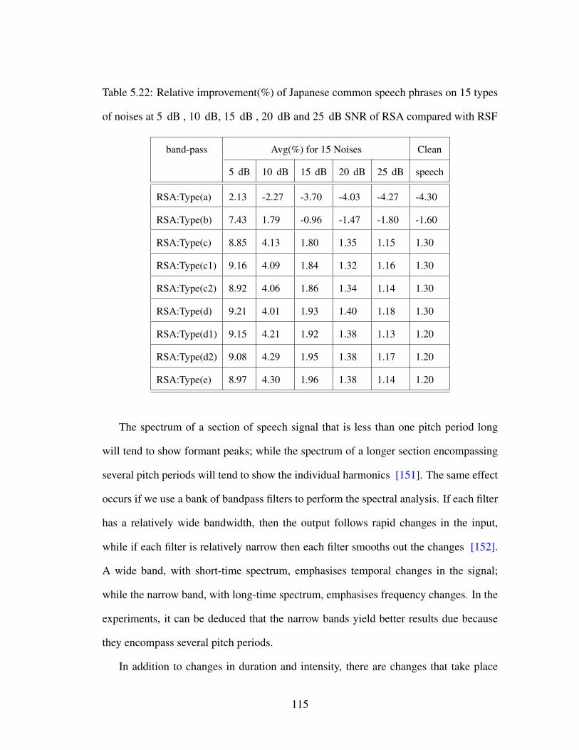
Table 5.22: Relative improvement(%) of Japanese common speech phrases on 15 types

of noises at 5 dB , 10 dB, 15 dB , 20 dB and 25 dB SNR of RSA compared with RSF

band-pass Avg(%) for 15 Noises Clean

5 dB 10 dB 15 dB 20 dB 25 dB speech

RSA:Type(a) 2.13 -2.27 -3.70 -4.03 -4.27 -4.30

RSA:Type(b) 7.43 1.79 -0.96 -1.47 -1.80 -1.60

RSA:Type(c) 8.85 4.13 1.80 1.35 1.15 1.30

RSA:Type(c1) 9.16 4.09 1.84 1.32 1.16 1.30

RSA:Type(c2) 8.92 4.06 1.86 1.34 1.14 1.30

RSA:Type(d) 9.21 4.01 1.93 1.40 1.18 1.30

RSA:Type(d1) 9.15 4.21 1.92 1.38 1.13 1.20

RSA:Type(d2) 9.08 4.29 1.95 1.38 1.17 1.20

RSA:Type(e) 8.97 4.30 1.96 1.38 1.14 1.20

The spectrum of a section of speech signal that is less than one pitch period long

will tend to show formant peaks; while the spectrum of a longer section encompassing

several pitch periods will tend to show the individual harmonics [151]. The same effect

occurs if we use a bank of bandpass filters to perform the spectral analysis. If each filter

has a relatively wide bandwidth, then the output follows rapid changes in the input,

while if each filter is relatively narrow then each filter smooths out the changes [152].

A wide band, with short-time spectrum, emphasises temporal changes in the signal;

while the narrow band, with long-time spectrum, emphasises frequency changes. In the

experiments, it can be deduced that the narrow bands yield better results due because

they encompass several pitch periods.

In addition to changes in duration and intensity, there are changes that take place

115

in the distribution of spectral energy over time such as modifications in the patterns of

the vowel formant frequencies or in the short-term spectra of speech features under the

influence of noise [153]. Including the change in the distribution of spectral energy

in the short-term spectra of various segments is advantageous in that it influences the

recognition accuracy positively.

A band-pass filter removes spectral components that occur at frequencies outside a

given range. In a segmented speech signal the high energy components become more

concentrated with increase in noise. In addition, signals long in time tend to be narrow

in spectrum. Applying a band-pass filter to a segmented noisy speech signal with a

narrow spectrum results in a minimal number of frequency components with reduced

amplitudes. These characteristics results in improved recognition accuracy under large

noise condition. However, the recognition accuracy on clean speech does not exhibit a

much higher improvement than the one obtained under noise conditions.

Most speech databases contain words of different sizes with energies concentrated

on different locations in the time domain. Some words are short and simple yet others

are long and complex. Applying a narrow band-pass to long and complex words may

cause such words to be modified resulting in negative effects. This effect may give rise to

much lower recognition accuracy results than expected. On the other hand, application

of a wide band-pass often results in both simple and complex words being adequately

handled. This in turn results in improved recognition accuracy.

Speech is periodic. The spectral analysis of any periodic signal shows a line spec-

trum. The spectral components occur only at frequencies which are whole-number mul-

tiples of the repetition frequency (harmonics) [152].

In this study, recognition accuracies calculated for 15 noises types have been shown

in tables and compared.

116

In the case of RSA, Table 5.21 shows that recognition accuracy increases with the

number of frequencies components applied for the respective noise level. The increase

in recognition accuracy rates with increase in frequency components used for training

is as reported in [145]. Results seem to suggest that increasing the number frequency

components can result in better speech recognition accuracy particularly when RSA is

adaptively applied.

5.2.7 Summary

Thisstudy presents a novel band-pass RSA filtering scheme using sets of filter banks

as a feature enhancement technique. Theoretical analysis indicates the proposed nar-

row band-pass and wide band-pass schemes are easy to realize and experimental re-

sults demonstrate their effectiveness of improving the robustness in automatic speech

recognition. The experiments also demonstrate that the width of band-pass scheme for

RSA has effects to noise suppressing. When band-pass is chosen reasonably, the al-

gorithm will have significant performance improvement. The improvement of accurate

rate (5dB) reaches 9.21 % for RSA Type(d) comparing with high-pass RSF IIR filtering

scheme.

117

Chapter 6

Discussion

6.1 Discussion

This chapter discusses findings of the experiments.

The performance of the proposed approach is assumed to be influenced by two main

factors: first, the level of noise and second the noise reduction technique being applied

on a particular noise. In general, speech recognition improves as signal-to-noise ra-

tio (SNR) is increased [154]. When people speak in a noisy environment, not only

does the loudness(energy) of their speech increase, the pitch and frequency compo-

nents also change. These speech variations are called the Lombard effect which in-

cludes a significant change in spectral tilt [155] [156] [157]. Some experimental stud-

ies done elsewhere indicate that these indirect influences of noise have a greater effect

on speech recognition than does the direct influence of noises entering microphones

[158] [159] [19].

The increase in recognition accuracy rates with increase in words used for training is

as reported by other researcher elsewhere [145]. In addition, just generically increasing

the vocabulary size can improve the accuracy for many common words but degrades the

118

recognition rate for less common words [146].

In the case of similar pronunciation phrases, the proposed approach show positive

results on ’genki”, “tenki” and “denki” with CMS/DRA. While slight improvements

are achieved on “kyu”, “juu” and “chuu”, with CMS/DRA at 20 dB and RSA at 10

dB, overall performance of the proposed approach shows improvement on 142 normal

phrases.

Different speakers may pronounce the same word differently in different contexts.

This is due to dialectal variations, educational qualifications and emotional conditions

and so on.

Mis-recognised words occur due to the absence of all pronunciation variations by

all speakers used in training which is the cause of the low performance of the speech

recognition system [160].

Vowel compression and expansion are mostly observed which are very difficult to

represent in the pronunciation dictionary [161] [162].

The use of TVLPC with FFT-based MFCC for feature extraction on Japanese speech

phrases has never been done before.

The proposed method performs slightly better on plosive phases “genki”, “denki”

and “tenki” than on “kyu”, “juu” and “chuu”.

It is observed that, in the case of clean speech, models 1 and 3 perform competitively

if not slightly better than model 0. This indicates that 1 or 3 dimensional components

may be adequate to realise better results with this proposed method. From the results, it

has been demonstrated that a single intra-frame cepstrum coefficient may be adequate to

improve recognition accuracy for 3 similar pronunciation phrases as well as on speech

uttered by elderly persons on clean speech. On the other hand, under similar conditions,

3 intra-frame cepstrum coefficients may be required to improve recognition accuracy in

119

the case of 142 words. Depending on the pronunciation context and the frequency of that

word also affects the accuracy of the system [147]. From the results, it can be inferred

that there is a difference in tendency between similar pronunciation phrases and phrases

uttered by elderly people. The recognition performance for speech influenced by noise

and distortion is particularly degraded when only very clean speech was used to train

the speech as was in this case. Secondly, poor performance in some of the proposed

models would be attributed to discontinuities of acoustic units around concatenation

points [149].

The cause of such low accuracy may be due to the distortion of the speech waveform

after noise reduction. RSA reduces more of unnecessary components with band-pass

characteristics. As the general dismal performance of proposed method, it is plausible

that the discontinuity at concatenation joints of acoustic units may be the cause, which

suggests need for smoothing techniques. Careful consideration is necessary in design-

ing such a filter. Excessive elimination of lower modulation frequency band may have

caused negative values in power spectrum and negative values lead to a problem when

power spectrum is converted to logarithmic power spectrum for obtaining cepstrum.

The challenge, however, is that the training costs of the word based HMM becomes

normally large. This means, in an event that one word is added to HMM speech model

database, many persons who utter target keywords several times, are often required. In

which case, we need a prior processing after a large set of speech database is prepared.

The accuracy of this approach increases with the number of reference speech wave-

forms (utterances) available for the reference words. It is observed that the proposed ap-

proach seems to be influenced by two main factors; first by the type of noise and second,

by the noise reduction technique being applied. It is also observed that the recognition

performance varies depending on the noise levels. It is also noted that models 1 and 3

120

perform competitively if not slightly better than model 0. This is an indication that 1 and

3 dimensional components may be adequate to realize better results with this proposed

method, although further optimization may be required.

By passing through a Mel filter bank, the number of dimensions of the feature

amount of mel frequency cepstrum is reduced and the load of calculation is reduced.

For the technique of speech recognition improvement, the researcher notes there is

a possibility of achieving higher accuracy if the best combination of filter with VAD

[163] and feature enhancement that incorporates noise and reverberation into audio-

logical speech-recognition testing are studied in order to improve predictions of perfor-

mance in the real world [164].

121

Chapter 7

Conclusion and Future Work

7.1 Conclusion

In this section an account of the results of this work is provided. In this work an en-

hanced robust ASR technique that exploits VAD, noise-reduction, and HMM-based

processing has been proposed. An attempt has been made to elucidate simulation re-

sults from a number of theory and mathematical analysis. Time varying speech features

and conventional FFT based MFCC features have been evaluated for a wide range of

simulation results. In chapter 2, a standard method of feature extraction as well as fea-

ture enhancement has been discussed. The complete pipeline for feature extraction and

the steps involved in identifying and recognizing a isolated word has also been shown.

The proposed ASR system has equally been discussed. The conventional MFCC fea-

ture extraction have been detailed and both the conventional TVLPC feature extraction

and the proposed feature estimation process have been explained using direct converted

TVLCP-based MFCC as well as feature estimation process using mel filtered TVLPC-

based MFCC. In the enhanced proposed method the inter-frame variation are combined

with intra-frame variation to realize the time varying speech features. The proposed fea-

122

ture model definition is equally discussed, showing the concatenation process of inter-

frame and intra-frame speech feature vectors. The significance of pattern recognition is

highlighted and ANN and HMM coding technologies have been discussed.

In chapter 3 VAD fundamentals covering short-time energy, short term autocorre-

lation and zero-crossing rate have been discussed. The short-time energy can detect

endpoint of voiced speech segment effectively. Short term autocorrelation can find re-

peating patterns, such as the presence of a periodic signal obscured by noise. The ZCR

can detect endpoint of voiceless speech segment effectively. The instantaneous pulse

noise can effect detection with short-time energy. This proposed approach that combine

use of short-time energy and zero-crossing rate helps improve accuracy of VAD.

In Chapter 4 The influence of additive and multiplicative noises have been discussed

and the modulation spectra concept and running spectrum analysis algorithm explained.

In this study,explainations have been made that in the time domain a speech signal and

environmental noise are additive. When such a signal is Fourier transformed, the addi-

tive noise can be removed in the frequency component. It has also been mentioned that

it is impossible for the multiplicative noises to successfully be removed using Fourier

transform only. A Fourier transform of a convolved signal makes it a multiplicative

signal which should be logarithmically transformed to realize an additive result. The

Fourier transform data from the specific time waveform is its modulation spectrum. The

influence of the additive noise causes the increase in energy. In addition, the system

noise has no time variation factor quite much compared with speech waveform. There-

fore, the modulation spectrum of speech usually concentrates its energy around or less

than 0 Hz.

Accordingly, the important part for speech recognition can be discriminated from

others on the modulation spectrum. RSA, CMS and DRA algorithms are introduced

123

to help minimize the problem of noise. Band-pass filtering using RSA is discussed in

greater detail. Additive noise components can be removed with band-pass filtering on

running spectrum domain to separate speech from noise. However, our study shows

that care should be taken in the design of such a band-pass filter. Excessive elimina-

tion of lower modulation frequency band may cause negative values in power spectrum

and negative values lead to a problem when power spectrum is converted to logarith-

mic power spectrum for obtaining cepstrum. However, the use of filter banks to sample

a number of higher frequency components in the modulation spectrum help improve

recognition accuracy. In compensating for distortions, we have used CMS as normal-

ization method and DRA to minimize the variability of noise feature values. In DRA,

each coefficient of a speech feature is adjusted proportionally to its maximum amplitude.

In Chapter 5 Two main experiments have been conducted. Experiment 1 focuses

on evaluating the performance of proposed time varying speech features with HMM. In

the first experiment simulation results for 3 similar pronunciation phrases, 13 phrases

uttered by elderly persons and the 142 normal phrases have been shown. The accuracy

of the approach increases with the number of reference speech waveforms (utterances)

available for the reference words. In other words, the average recognition accuracy is

higher for the 142 normal phrases compared to that of the 3 similar phrases. It has been

observed that the proposed approach seems to be influenced by two main factors; first

by the type of noise and second, by the noise reduction technique being applied. It has

also been observed that the recognition performance varies depending on the noise lev-

els. Overall, the proposed method performs slightly better on plosive phrases “genki”,

“denki” and “tenki” than on “kyu”, “juu” and “chuu”. It is also noted that models 1 and

3 perform competitively if not slightly better than model 0. This is an indication that 1

and 3 dimensional components may be adequate to realize better or slightly better results

124

with this proposed method. Using few components reduces the computation time on the

part of TVLPC. The second experiment focuses on the use of band-pass RSA FIR filter-

ing scheme on FFT-based MFCC. In continuous speech recognition RSA is applied for

the high frequency component while eliminating noise and retaining important speech

characteristics in the modulation spectrum. In addition, its merits have been found for

the phrase recognitionl. 9 band-pass filter banks were evaluated with varying number of

frequency components. The same were compared to the performance of high-pass RSF

IIR filtering scheme under 5 noise levels of 5 , 10 dB, 15 dB, 20 dB 25 dB and ∞. The

relative improvement (%) on the 15 types of noises were 9 %, 4 %, 1.9 %, 1.3 %, 1.1

%, and 1.3 % respectively on 100 Japanese common speech phrases uttered by 30 male

speakers and each phrase repeated three times (9000 waveforms).

In chapter 6, the results obtained from proposed time varying speech features and

conventional approach have been evaluated. Even if the proposed method does not

require many time varying components for each spoken word or phrase and can use

a small number of speech waveforms as references, there is a difference in tendency

between similar pronunciation phrases and phrases uttered by elderly people. The ten-

dency shows better results for elderly people compared with similar phrases. It can be

inferred that the dismal performance of some cases could be attributed to discontinuities

of acoustic units around concatenation points. Even if care may be taken in designing

the RSA band-pass filter there may be unnecessary components. It has been found that

concatenating FFT-based MFCC with the TVLPC-based MFCC to create time varying

speech features (TVSF) can improve the speech recognition capability for some HMM

implementations. The proposed method may be a simpler solution for speech recogni-

tion applications.

In summary, two kinds of TVLPC features can be realized; the time invariant and

125

time varying type. Model 1 and model 3 of TVSF algorithm improves the recognition

accuracy of ASR. Overall, CMS/DRA approach is better than others in low SNR. In-

crease in the number of words shows a corresponding increase in recognition accuracy.

7.2 Future work

Although this proposed method has improved the performance of ASR system with time

varying speech features, the recognition accuracy is not so high in low SNR. The real

environment is sophisticated and extremely unpredictable, an attempt must therefore be

made to improve further the recognition accuracy of ASR system in order for such a

system to be ideal for practical application.

The VAD algorithm need to be modified and thus improved accuracy of endpoint

detection. Use of short-time energy method is limited to detect endpoint in low SNR.

Hence, continued research and exploring of new and enhanced technology in order to

detect endpoint accurately in low SNR are required. As an immediate alternative, the

use of a combination of VAD techniques requires consideration.

Since the recognition accuracy recognition seems to be influenced by the type of

noise and possibly the discontinuities of acoustic units around concatenation points,

smoothing techniques should be explored. In addition, an attempt should be made to

improve the performance of RSA in low SNR by conducting further experiments under

various conditions to ascertain the ideal and practical pass-band.

The accuracy increases with an increasingly large reference waveform database. The

future work will attempt to find the best compromises between accuracy and computa-

tion time. The proposed method is based on the small vocabulary of 3 and 142 normal

words. Although models 1 and 3 perform well, on some RSA, it is still low when the

126

method is applied to small vocabulary of 3 phrases. Hence the need to modify RSA

algorithm and an attempt to decrease computation time of TVLCP, with the aim of im-

proving the recognition accuracy.

Further improvement in the feature extraction using TVSF will be sought. Also

implementing the proposed approach in other languages such as C/C++ that are much

faster than MATLAB will be considered. In addition, a computer with a much faster

processing speed would be an important factor considering that speech processing is

quite demanding assuming that slow processing may be a contributing factor to low

results in some instances.

127

Bibliography

[1] Samudravijay K, “Speech and Speaker Recognition: a tutorial, http://speech.

tifr.res.in/chief/publ/03iwtdil_spSpkrReco.pdf, viewed on 26 Oct.

2016.

[2] Santosh K.Gaikwad, Bharti W.Gawali, and Pravin Yannawar, “A Review on Speech

Recognition Technique,” International Journal of Computer Applications(0975

8887), vol.10, no.3, Nov. 2010.

[3] Dennis H. Klatt, “Speech perception: a model of acoustic-phonetic analysis and

lexical access: Theoretical Perspectives,” Journal of Phonetics, vol.7, pp.279-312,

1979.

[4] Carol Yvonne Espy-Wilson, “ An Acoustic-Phonetic Approach to Speech Recogni-

tion: Application to the Semivowels”, RLE Technical Report, no.531, Jun. 1987.

[5] R. Schwartz, Y. Chow, O. Kimball, S. Roucos, M. Krasner and J. Makhoul,

“Context-dependent modeling for acoustic-phonetic recognition of continuous

speech,” IEEE International Conference on Acoustics, Speech, and Signal Process-

ing, ICASSP ’85, Apr. 1985.

[6] “Speech Recognition in Machines,” http://www.ece.ucsb.edu/Faculty/

Rabiner/ece259/Reprints/mitecs_paper.pdf, viewed on 26 Oct. 2016.

128

[7] F. Itakura,“Minimum prediction residual principle applied to speech recognition,”

IEEE Transactions on Acoustics, Speech, and Signal Processing, vol.23, no.1,

pp.67-72, Feb. 1975.

[8] L.R. Rabiner,“A tutorial on hidden Markov models and selected applications in

speech recognition,” Proceedings of the IEEE, vol.77, no. 2, pp.257-286, Feb. 1989.

[9] Lawrence Rabiner, and Biing-Hwang Juang, “ Fundamentals of speech recogni-

tion,” Prentice-Hall, Inc. Upper Saddle River, NJ, USA, 1993.

[10] D.R. Reddy, “An Approach to Computer speech Recognition by direct analysis of

the speech wave,” Tech. Report No.C549, Computer Science Department, Stanford

University, Sept. 1996.

[11] C.S. Myers and L.R. Rabiner, “ A Level Building Dynamic Time Warping Al-

gorithm for Connected Word Recognition” IEEE Trans. Acoustics, Speech Signal

Proc., ASSP-29, pp.284-297, Apr. 1981.

[12] L. R. Rabiner, S. E. Levinson and M. M. Sondhi,“On the application of Vector

Quantization and Hidden Markov Models to speaker-independent, isolated word

recognition,” The Bell System Technical Journal, vol.62, no.4, Apr. 1983.

[13] Tavel R.K. Moore,“Twenty things we still dont know about speech,” Proc.

CRIM/FORWISS Workshop on Progress and Prospects of speech Research and

Technology, 1994.

[14] Keh-Yih Su and Chin-Hui Lee, “Speech Recognition using weighted HMM and

subspace projection approaches,”IEEE Transactions on Speech and Audio Process-

ing, vol.2, no.1, pp.69-79, Jan. 1994.

129

[15] Nicols Morales, John H. L. Hansen and Doorstep T. Toledano, “MFCC Compen-

sation for improved recognition filtered and band limited speech, Center for Spoken

Language Research, University of Colorado at Boulder, Boulder (CO), USA.

[16] M.A. Anusuya and S.K. Katti, Speech Recognition by Machine: A Review, Inter-

national Journal of Computer Science and Information Security, 2009.

[17] John Butzberger, “Spontanious Speech Effect in Large Vocabulary speech recog-

nition application,” SRI International Speech Research and Technology program,

Menlo Park, CA, 94025, USA.

[18] Shigeru Katagiri and Chin-Hui Lee, “A New hybrid algorithm for speech recogni-

tion based on HMM segmentation and learning Vector quantization,” IEEE Trans-

actions on Speech and Audio Processing, vol. 1, no.4, pp.421-430, Oct. 1993.

[19] Sadaoki Furui, “Towards Robust Speech Recognition Under Adverse Condi-

tions,” Proc. ESCA Workshop on Speech Processing in Adverse Conditions, Cannes-

Mandeliue, France, Nov. 10-13, 1992.

[20] https://en.wikipedia.org/wiki/Lombard_effect, viewed on 26 Nov.

2016.

[21] Junqua JC, “The Lombard reflex and its role on human listeners and automatic

speech recognizers,” Journal of the Acoustical Society of America, vol.93 no.1,

pp.51024, Jan. 1993.

[22] Sadaoki Furui, “Digital Speech Processing, Synthesis, and Recognition” CRC

Press; 2nd edition, 2000.

[23] https://en.wikipedia.org/wiki/Speech_recognition, Retrieved 14 De-

cember 2016.

130

[24] Wayne A. Lea, “ Trends in Speech Recognition,” Prentice Hall, 1980.

[25] Masumi Watanabe, Hiroshi Tsutsui, and Yoshikazu Miyanaga,“Robust speech

recognition for similar pronunciation phrases using MMSE under noise environ-

ments,” Proc. 13th International Symposium on Communications and Information

Technologies (ISCIT), 2013.

[26] J. Tierney, “A study of LPC analysis of speech in additive noise,” IEEE Trans.

on Acoustic., Speech, and Signal Process., vol. ASSP-28, no.4, pp.389-397, Aug.

1980.

[27] S.M. Kay,“Noise compensation for autoregressive spectral estimation,” IEEE

Trans. on Acoust., Speech, and Signal Process., vol. ASSP-28, no.3, pp.292-303,

Mar. 1980.

[28] Pramod B. Patil, “Multilayered Network for LPC based Speech Recognition,”

IEEE, 1998.

[29] Mark G. Hall, Alan V. Oppenheim, and Alan S. Willsky,“Time-varying parametric

modelling of speech,” Signal Processing, vol.5, pp.267-285, 1983.

[30] Safdar Tanweer, Abdul Mobin, and Afshar Alam,“Analysis of Combined use of

NN and MFCC for Speech Recognition,”International Journal of Computer, Elec-

trical, Automation, Control and Information Engineering, vol.8, no.9, 2014.

[31] L. Muda M. Begam, I. Elamvazuthi, “Voice recpgnition algorithm using Mel Fre-

quency Cepstral Coefficient (MFCC) and Dynamic Time Warping (DTW) tech-

niques,” Journal of Computing, vol.2, no.3, pp.138-143, 2010.

[32] Chadawan Ittichaichareon, Siwat Sukasri and Tha-Weesak Yingthawornsuk,“

Speech recognition using MFCC,” Proc. International conference on computer

131

Graphics simualtion and modeling (ICGSM 2012) July 28-29 2012 pattaya, Thai-

land.

[33] Anjali Bala, Abhijeet Kumar, Niddhika Birla,“Voice command recognition sys-

tem based on MFCC and DTW,” International Journal of Engineering Science and

Technology, vol.2, no.12, pp.7335-7342, 2010.

[34] Petr Motlicek, “ Feature Extraction in speech coding and recognition,” Report

of PhD research internship in ASP Group, OGI-OHSU, 2002, http://www.fit.

vutbr.cz/~motlicek/publi/2002/rp.pdf, viewed on 26 Oct. 2016.

[35] Vikhyath Narayan K N, and S P Meharunnisa, “Detection and Analysis of Stut-

tered Speech ,” International Journal of Advanced Research in Electronics and

Communication Engineering (IJARECE) vol.5, no.4, Apr., 2016.

[36] Urmila Shrawankar and Dr. Vilas Thakare, “ Techniques for feature extraction in

speech recognition system: a comparative study,” PG Dept. of Computer Science,

SGB Amravati University, Amravati.

[37] G. Kang and S. Guo,“Variable Sliding Window DTW Speech Identification Algo-

rithm,” Proc. The 9th International Conference on Hybrid Intelligent Systems, vol.

1, pp.304-307, Aug. 2009.

[38] Dan Jurafsky and James H. Martin, Speech and Language Processing: An Intro-

duction to Natural Language Processing, Computational Linguistics, and Speech

Recognition,Prentice Hall,2009.

[39] Peter Foster and Thomas Schalk, Speech Recognition The Complete Practical Ref-

erence Guide,CMP Books,1993.

132

[40] Kuldip K. Paliwal, Automatic speech and speaker recognition: advanced topics,

Springer, 1996.

[41] Xuedong Huang and Alejandro Acero and Alex Acero and Hsiao-Wuen Hon,

Spoken language processing: a guide to theory, algorithm, and system develop-

ment,Upper Saddle River, NJ: Prentice Hall,2001.

[42] Lawrence Rabiner and Biing-Hwang Juang, Fundamentals of speech recogni-

tion,Prentice Hall PTR,Upper Saddle River, New Jersey, USA,1993.

[43] K.V. Krishna Kishore, P. Krishna Satish, “Emotion Recognition in speech using

MFCC and Wavelete Features”, 3rd IEEE International Advance Computing Con-

ference

[44] J. SirishaDevi, Dr. Srinivas Yarramalle, Siva Prasad Nandyala,“Speaker Emotion

Recognition Based on Speech Features and Classification Techniques,” I.J. Image,

Graphics and Signal Processing, vol.7, pp. 61-77, Jun. 2014.

[45] Juan Ignacio Godino Llorente, Pedro G omez-Vilda, and Manuel Blanco-

Velasco,“Dimensionality Reduction of a Pathological Voice Quality Assessment

System Based on Gaussian Mixture Models and Short-Term Cepstral Parameters’,

IEEE Transactions on Biomedical Engineering, vol.53, no. 10, Oct. 2006.

[46] Sahar E. Bou-Ghazale and John H.L. Hansen ,“A comparative study of traditional

and newly proposed features for recognition of speech under stress,” IEEE Trans.

Speech Audio Process., vol.8, no.4, pp.429-442, Jul. 2000.

[47] B. S. Atal,“Effectiveness of linear prediction characteristics of the speech wave for

automatic speaker identification and verification,” Journal of the Acoustical Society

of America, vol.55, no.6, pp.1304-1312, Jun. 1974.

133

[48] F. Itakura,“Line spectrum representation of linear predictive coefficients of speech

signals,” Journal of the Acoustical Society of America, vol.57, no.S1, pp.S35, Mar.

2000.

[49] B.S. Atal,“Automatic recognition of speakers from their voices,” Proceedings of

the IEEE, vol.64, no.4, pp.460-475, Apr. 1976.

[50] Hong Kook Kim and Seung Ho Choi and Hwang Soo Lee,“On approximating line

spectral frequencies to LPC cepstral coefficients,” IEEE Transactions on Speech and

Audio Processing, vol.8, no.2, pp.195-199, Mar. 2000.

[51] Steven B. Davis. and Paul Mermelstein,“Comparison of parametric representations

for monosyllabic word recognition in continuously spoken sentences,” IEEE Trans-

actions on Acoustics, Speech and Signal Processing, vol.28, no.4, pp.357-366, Aug.

1980.

[52] Hynek Hermansky,“Perceptual linear predictive (PLP) analysis of speech,” Journal

of the Acoustical Society of America, vol.87, no.4, pp.1738-1752, Apr. 1990.

[53] Hermansky, H. and Cox, L.A., Jr.“Perceptual Linear Predictive (PLP) Analysis-

Resynthesis Technique,” IEEE Workshop on Applications of Signal Processing to

Audio and Acoustics, pp.37-38, Oct. 1991.

[54] Bojan Petek and Joe Tebelskis, “Context-Dependent Hidden Control Neural Net-

work Architecture for Continuous Speech Recognition”, Proceeding IEEE Interna-

tional Conference on Acoustics, Speech and Signal Processing, 1992.

134

[55] Eslam Mansour mohammed, Mohammed Sharaf Sayed, Abdallaa Mohammed

Moselhy and Abdelaziz Alsayed Abdelnaiem, “LPC and MFCC Performance Eval-

uation with Artificial Neural Network for Spoken Language Identification”, Inter-

national Journal of Signal Processing, Image Processing and Pattern Recognition,

vol.6, no.3, Jun. 2013.

[56] Harvey Fletcher, “Auditory patterns,” Reviews of Modern Physics 12, 47, Bell Tele-

phone Laboratories, New York, 1940. ]

[57] https://en.wikipedia.org/wiki/Window_function, viewed on 21 October

2016.

[58] Curtis Roads (2002), Microsound, The MIT Press. 2002.

[59] https://www.dsprelated.com/freebooks/sasp/Hann_Hanning_Raised_

Cosine, viewed on 27 oct 2016.

[60] Kshitiz Kumar, Chanwoo Kim and Richard M. Stern, “Delta-spectral cepstral co-

efficients for robust speech recognition,” Department of Electrical and Computer

Engineering, Language Technologies Institute, Carnegie Mellon University, Pitts-

burgh, PA 15213.

[61] D.K. Faddeev and V.N. Faddeeva, Computational Methods of Linear Algebra,

W.H. Freeman and Co., San Francisco, 1963.

[62] R. Pieraccini, “Pattern compression in isolated word recognition,” Signal Process-

ing, vol.7, no.1, pp.1-15, Sep. 1984.

[63] S. Lalitha, D. Geyasruti, R. Narayanan, and M. Shravani,“Emotion Detection us-

ing MFCC and Cepstrum Features,”4th International Conference on Eco-friendly

Computing and Communication Systems, 2015.

135

[64] Mehmet S. Unluturk, Kaya Oguz, Cskun Atay,“Emotion Recognition Using Neu-

ral Networks”, Word Academy of Science, Engineering and Technology, vol.7, no.3,

2013.

[65] B H Juang,“On the hidden Markov model and dynamic time warping for speech

recognition: A unified view,” AT&T Technical journal, vol.63. no.7, pp.1213-1243,

1984.

[66] X. D. Huang and Y. Ariki and Mervyn A. Jack, Hidden Markov Models for Speech

Recognition, Edinburgh University Press, 1990.

[67] Yoshizawa, S. and Miyanaga, Y. and Yoshida, N,“On a High-Speed HMM VLSI

Module with Block Parallel Processing,” Institute of Electronics Information and

Communication Engineers, vol.J85-A, no.12, pp.1440-1450, Feb. 2002.

[68] J.Ramirez, J.M Gorriz and J.C. Segura, Robust Speech Recognition and Under-

standing ,I-tech Education and Publishing, 2007.

[69] D. K. Freeman, G. Cosier, C. B. Southcott, and I. Boyd, “The voice activity detec-

tor of the pan-European digital mobile telephone service”,Proc. IEEE, vol. CH2673-

2, 1989.

[70] A. Sangwan, M.C. Chiranth, H.S. Jamadagni, R. Sah, R. Venkatesha Prasad and

V. Gaurav, “VAD techniques for real-time speech transmission on the Internet,” 5th

IEEE International Conference on High Speed Networks and Multimedia Commu-

nication (Cat. No.02EX612), 2002.

[71] K. Itoh and M. Mizushima, “Environmental Noise Reduction Based on

Speech/Non-Speech Identification for Hearing Aids,” IEEE Computer Society,

vol.1, no. , pp. 419, 1997.

136

[72] Rashmi Makhijani ,Urmila Shrawankar, and Dr. V. M. Thakare, “Speech enhance-

ment using pitch detection approach for noisy environment,” International Journal

of Engineering Science and Technology (IJEST), vol.3 no.2 Feb. 2011.

[73] M. Marzinzik and B. Kollmeier,“Speech pause detection for noise spectrum esti-

mation by tracking power envelope dynamics,” IEEE Transactions on Speech and

Audio Processing, vol.10, no.2, Aug. 2002.

[74] F. Gouyon, F. Pachet, and O. Delerue,“Classifying percussive sounds: a matter of

zero-crossing rate,” in Proceedings of the COST G-6 Conference on Digital Audio

Effects (DAFX-00), Verona, Italy, December 79, 2000.

[75] https://en.wikipedia.org/wiki/Zero-crossing_rate, viewed on 30 Oc-

tober 2016.

[76] R. Tucker, “Voice activity detection using a periodicity measure,” IEE Proceedings

I - Communications, Speech and Vision, vol.139, no.4, Aug. 1992.

[77] S.G. Tanyer, and H. ’Ozer, “Voice activity detection in nonstationary noise,” IEEE

trans on speech and audio processing, vol.8, no.4, pp.478-482, 2000.

[78] Doh-Suk Kim, Soo-Young Lee, and Rhee M. Kil,“Auditory Processing of Speech

Signals for Robust Speech Recognition in Real-World Noisy Environments,” IEEE

Transactions on Speech and audio processing, vol.7, no.1, Jan. 1999.

[79] http://spib.linse.ufsc.br/noise.html, viewed on 5 Nov. 2016.

[80] Junqua, Jean-Claude, Haton and Jean-Paul, Robustness in Automatic Speech

Recognition: Fundamentals and Applications, Springer, 1996.

137

[81] Yifan Gong,“Speech recognition in noisy environments: A survey,” Speech Com-

munication, vol.16, no.3, pp.261-291, Apr. 1995.

[82] B. Raj,V.N. Parikh, and R.M. Stern,“The effects of background music on speech

recognition accuracy,” IEEE International Conference on Acoustics, Speech, and

Signal Processing, vol.2, no.2, pp.851-854, Apr. 1997.

[83] Veronique Stouten, Hugo Van hamme and Patrick Wambacq,“Joint Removal of

Additive and Convolutional Noise with Model-Based Feature Enhancement,” In

Proc. International Conference on Acoustics, Speech and Signal Processing, vol.1,

pp.949-952, May 2004.

[84] A. Acero, L. Deng, T. Kristjansson, and J. Zhang, “HMM adaptation using Vector

Taylor Series for noisy speech recognition, in Proc.ICSLP, pp.869872. Oct. 2000.

[85] Hynek Hermansky, Nelson Morgan, and Hans-Gunter Hirsch,“Recognition of

speech in additive and convolutional noise based on RASTA spectral processing,” in

Proc. IEEE International Conference on Acoustics, Speech, and Signal Processing

ICASSP, vol.2, pp.83-86, Apr. 1993.

[86] Joachim Koehler, Nelson Morgan, Hynek Hermansky, H. Guenther

Hirsch,and Grace Tong,“Integrating RASTA-PLP into Speech Recognition,”

in Proc.ICASSP94, vol.1, pp.421-424, Apr. 1994.

[87] B H Juang and L R Rabiner and J G Wilpon,“On the use of bandpass liftering in

speech recognition,” IEEE Transactions on Acoustics, Speech and Signal Process-

ing, vol.35, no.7, pp.947-954, Jul. 1987.

138

[88] N. Erdol, C. Castelluccia and A. Zilouchian,“Recovery of missing speech packets

using the short-time energy and zero-crossing measurements,” IEEE Transactions

on Speech and Audio Processing, vol.1, no.3, pp.295-303, Jul. 1993.

[89] http://www.azimadli.com/vibman/stationarysignals.htm, viewed on 22

Nov. 2016.

[90] L.R. Rabiner and R.W.Schafer,Digital Processing of Speech Signals,Rainbow-

Bridge Book Company PTR,Upper Saddle River, Prentice HallUSA,1978.

[91] S. Seneff, “Real-time harmonic pitch detector,” IEEE Transactions on Acoustics,

Speech and Signal Processing, vol.26. no.4, pp.358-365, Aug. 1978.

[92] L R Rabiner and M R Sambur, “An Algorithm for Determining the Endpoints for

Isolated Utterances” The Bell System Technical Journal, vol.54, no.2, pp.297-315,

1975.

[93] J. C. Junqua, B. Mak and B, Reaves,“A robust algorithm for word boundary detec-

tion in the presence of noise,” IEEE Transactions on Speech and Audio Processing,

vol.2, no.3, pp.406-412, Jul. 1994.

[94] Gang Xu and Bo Tong and XiaoWei He, “Robust Endpoint Detection in Mandarin

Based on MFCC and Short-Time Correlation Coefficient,” International Conference

on Intelligent Computation Technology and Automation, vol.2, pp.336-339, Oct.

2009.

[95] Yiu-Kei Lau and Chok-Ki Chan,“Speech recognition based on zero crossing rate

and energy,” IEEE Transactions on Acoustics, Speech and Signal Processing,vol.33,

no.1, pp.320-323, Feb. 1985.

139

[96] Gan, C.K. and Donaldson, R.W.“Adaptive silence deletion for speech storage and

voice mail applications,” IEEE Transactions on Acoustics, Speech and Signal Pro-

cessing, vol.36, no.6, pp.924-927, Jun. 1988.

[97] Zhang, T. and Kuo, C.-C.Jay,“Audio content analysis for online audiovisual data

segmentation and classification,” IEEE Transactions on Speech and Audio Process-

ing, vol.9, no.4, pp.441-457, May 2001.

[98] Panagiotakis, C. and Tziritas, G.,“A speech/music discriminator based on RMS

and zero-crossings,”IEEE Transactions on Multimedia, vol.7, no.1, pp.155-166,

Feb. 2005.

[99] Naoya Wada, Noruba Hayasaka, Shingo Yoshizawa and Yoshikazu Miyanaga, “

Direct Control on Modulation Spectrum for Noise-Robust Speech Recognition and

Spectral Subtraction”, IEEE, pp. 2533-2536, 2006.

[100] Yifan Gong, “ Speech recognition in noisy environments: A survey ,”, Speech

Communication, vol. 16, pp. 261-291, Nov. 1994.

[101] J. A. Nolazco Flores and S. J. Young, “Continuous Speech Recognition in Noise

Using Spectral Subtraction and HMM Adaptation,” ICASSP Pp.I. (1994) pp. 409-

412, 1994.

[102] J. A. Nolazco Flores and S. J. Young, “ Adapting a HMM-based Recogniser for

Noisy Speech Enhanced by Spectral Subtraction,” CUED/F-INFENG/TR.123, Apr.

1993.

[103] K. Yao, K. K. Paliwal and S. Nakamura, “Model-based noisy speech Recognition

with Environment Parameters Estimated by noise adaptive speech Recognition with

140

prior,” EUROSPEECH 2003-GENEVA, Switzerland, Tech. Rep., pp. 1273-1276,

2003.

[104] M. Westphal, “The Use of Cepstral Means in Conversational Speech Recogni-

tion,” Interactive Systems Laboratories, University of Karlsruhe, 76128, Karlsruhe,

Germany.

[105] S. Dharanipragada, U. H. Yapanel, and B.D. Rao, “Robust Feature Extraction for

Continuous speech Recognition using the MVDR Spectrum Estimation method,”

vol. 15, no. 1, pp.224-234, Jan. 2007.

[106] Rahim, M.G. and Biing-Hwang Juang and Wu Chou and Buhrke,

E.,“Effectiveness of linear prediction characteristics of the speech wave for

automatic speaker identification and verification,” Journal of the Acoustical Society

of America, vol.55, no.6, pp.1304-1312, 1974.

[107] Naik, D.,“Pole-filtered cepstral mean subtraction,” International Conference on

Acoustics, Speech, and Signal Processing, vol.1, no.1, pp.157-160, May 1995.

[108] Rahim, M.G. and Biing-Hwang Juang and Wu Chou and Buhrke, E.,“Signal con-

ditioning techniques for robust speech recognition,” IEEE Signal Processing Let-

ters, vol.3, no.4, pp.107-109, Apr. 1996.

[109] Z.H. Chen, and Y.F. Liao, and Y.T. Juang, ,“Eigen-prosody analysis for robust

speaker recognition under mismatch handset environment,” Electronics Letters,

vol.40, no.19, pp.1233-1235, Sep. 2004.

[110] Shabtai, N.R. and Zigel, Y. and Rafaely, B.,“The Effect of GMM Order and CMS

on Speaker Recognition with Reverberant Speech,”Hands-Free Speech Communi-

cation and Microphone Arrays, PP.144-147, May 2008.

141

[111] Y. Sun, K. Ohnuki, and Y. Miyanaga, “On the Use of RSA and DRA to Improve

the Robustness of Continuous Speech Recognition Systems in Adverse Conditions,”

IEEE International Symposium on Communications and Information Technology,

ISCIT 2010, pp. 28-33, 2010.

[112] S Yoshizawa and N Wada and N Hayasaka and Y Miyanaga,“Noise robust speech

recognition focusing on time variation and dynamic range of speech feature param-

eters,” International Symposium on Intelligent Signal Processing and Communica-

tion Systems (ISPACS),pp.484-487, Dec. 2003.

[113] Naoya Wada and Shingo Yoshizawa and Noboru Hayasaka and Yoshikazu-

Miyanaga, “Robust Speech Feature Extraction using RSF/DRA and Burst Noise

Skipping,” Transactionson Electrical Engineering, Electronics, and Communica-

tions ECTI-EEC, vol.3, no.2, pp.100-107, Aug. 2005.

[114] Naoya Wada and Noboru Hayasaka and Nobuo Hataoka and Yoshikazu

Miyanaga,“Noise Robust Speech Detection/Recognition System Including

RSF/DRA and MFCC International Symposium on Communications and Informa-

tion Technologies (ISCIT), vol.1, pp. 455-458, Sep. 2003.

[115] Noboru Hayasaka, Shingo Yoshizawa, and Yoshikazu Miyanaga, “Robust speech

recognition with feature extraction using combined method of RSF and DRA,” Int’l

Symposium on Communications and Information Technologies (ISCIT), pp.1001-

1004, Oct. 2004.

[116] Noboru Hayasaka and Yoshikazu Miyanaga, “Spectrum filtering with FRM for

robust speech recognition,” IEEE International Symposium on Circuits and Systems

(ISCAS), pp.3285-3288, May 2006.

142

[117] Noboru Hayasaka, Nobuo Hataoka, and Yoshikazu Miyanaga, “Noise robust

speech detection/recognition system including RSF/DRA and MFCC,” Int’l Sym-

posium on Communications and Information Technologies, (ISCIT), pp.455-458,

Sep. 2003.

[118] M. Sakata, Y. Miyanaga and N. Yoshida, “A new design method of Band-pass

Fileters Based on a Frequency-Response-Masking Technique,” Proc. International

Symposium on Intelligent Signal Processing and Communication, Dec. 2003.

[119] S. Yoshizawa, N. Wada, N. Hayasaka and Y. Miyanaga, “ Hardware Implemen-

tation of a Noise Robust Speech Recognition System Using RSF/DRA Technique,”

Technical report of IEICE, CAS2003-42, pp.127-132, June 2003.

[120] K. Fujioka, and Y. Miyanaga,“A new noise reduction method of speech signal

with running spectrum filtering,” International Symposium on Intelligent Signal

Processing and Communication Systems, pp. 173-176, Nov. 2004.

[121] Hayasaka, Noboru and Khankhavivone, Kham and Miyanaga, Yoshikazu and

Songwatana, Kraisin, “New Robust Speech Recognition By Using Nonlinear Run-

ning Spectrum Filter,”International Symposium on Communications and Informa-

tion Technologies,pp. 133-136, Oct. 2006.

[122] Q. Zhu, N. Ohtsuki, Y. Miyanaga, and N. Yoshida,“Robust speech analysis in

noisy environment using running spectrum filtering,” International Symposium on

Communications and Information Technologies, vol. 2, pp. 995-1000, Oct. 2004.

[123] N. Wada, N. Hayasaka, S. Yoshizawa, and Y. Miyanaga, “Robust speech recog-

nition with feature extraction using combined method of RSF and DRA,” Interna-

tional Symposium on Communications and Information Technologies, vol. 2, pp.

143

1001-1004, Oct. 2004.

[124] N. Hayasaka, and Y. Miyanaga,“Spectrum filtering with FRM for robust speech

recognition,” IEEE International Symposium on Circuits and Systems, pp. 3285-

3288, Nov. 2006.

[125] N. Ohtsuki, Qi Zhu and Y. Miyanaga, “The effect of the musical noise suppres-

sion in speech noise reduction using RSF,” International Symposium on Communi-

cations and Information Technologies, vol. 2, pp. 663-667, Oct. 2004.

[126] Yang Jie and Wang Zhenli, “Noise robust speech recognition by combining

speech enhancement in the wavelet domain and Lin-log RASTA,” International

Colloquium on Computing, Communication, Control, and Management, vol. 2, pp.

415-418, Aug. 2009.

[127] M Holmberg and D Gelbart and W Hemmert,“Automatic speech recognition with

an adaptation model motivated by auditory processing,” IEEE Transactions on Au-

dio, Speech, and Language Processing, vol. 14, no. 1, pp. 43-49, Jan. 2006.

[128] M Grimaldi and F Cummins,“Speaker Identification Using Instantaneous Fre-

quencies,” IEEE Transactions on Audio, Speech, and Language Processing, vol. 16.

no. 6, pp. 1097-1111, Aug. 2008.

[129] H. Hermansky and N. Morgan, “RASTA processing of speech,” IEEE Trans. on

Speech and Audio Proc., vol. 2, no. 4, pp. 578-589, Oct. 1994.

[130] N. Hayasaka, S. Yoshizawa, N. Wada, Y. Miyanaga and N. Hataoka, “A Study of

Robust Speech Recognition System and Its LSI Design,”The Society of Instrument

and Control Engineers, vol. 41, no. 5, pp. 473-480, May 2005.

144

[131] Lawrence R. Rabiner and Ronald W. Schafer, “Theory and Application of Digital

Speech Processing,” Prentice-Hall Inc., 2009.

[132] Alan V. Oppenheim and Ronald W. Schafer and John R. Buck, “Discrete-time

Signal Processing,” 2nd, Prentice-Hall Inc.,1998.

[133] L. R. Rabiner and R. W. Schafer,“Introduction to Digital Speech Processing,”

Foundations and Trends in Signal Processing, vol. 1, no. 1-2, pp. 1-194, 2007.

[134] Johan de Veth and Louis Boves,“Channel normalization techniques for automatic

speech recognition over the telephone,” Speech Communication, vol. 25, no. 1, pp.

149-164, 1998.

[135] Noboru Kanedera, Takayuki Arai, Hynek Hermansky and Misha Pavel, “On the

importance of various modulation frequencies for speech recognition,” Proceedings

of EUROSPEECH 97, Rhodos, Greece, Sep. 1997.

[136] Hynek Hermansky, Eric Wan, and Carlos Avendano, “Speech enhancement based

on temporal processing,” IEEE International Conference on Acoustic, Speech and

Signal Processing, Detroit, Michigan, Apr.1995.

[137] Carlos Avendano, Sarel van Vuuren and Hynek Hermansky, “On the properties

of temporal processing for speech in adverse environments,” Proceedings of 1997

Workshop on Applications of Signal Processing to Audio and Acoustics, Mohonk

Mountain House, New Paltz, New York, October 18-22, 1997.

[138] W. Ohnuki, K. Takahashi, S. Yoshizawa, and Y. Miyanaga, “Analysis of Robust-

ness of RSA acoustic model by distance between Phonemes,” IEICE Tech. Rep.,

vol.109, no.112, SIP2009-25, pp. 37-42, Jul. 2009.

145

[139] N. Wada, N. Hayasaka, and Y. Miyanaga, “Robust speech Recognition with Fea-

ture Extraction using Combined method of RSF and DRA,” in IEEE International

Symposium on Communications and Information Technology (ISCIT), vol. 2, pp.

1001-1004, Apr. 2004.

[140] D. Sanjib, “Speech Recognition Technique: A Review,” International Journal of

Enginering Research and Applications, vol. 2, no. 3, pp. 2071-2087, 2012.

[141] B. Anjali, K. Abhijeet, and B. Nidhika, “Voice Command Recognition System

Based on MFCC and DTW,” International Journal of Engineering Science and

Technology, vol. 2 no. 12, pp. 7335-7342, 2010.

[142] Daniel Rudoy,Thomas F. Quatieri,Patrick J. Wolfe, “Time-Varying Autoregres-

sive Tests for Multiscale Speech Analysis,” INTERSPEECH, ISCA 2009, 6-10, Sep.

2009.

[143] http://www.speech.cs.cmu.edu/comp.speech/Section1/Data/noisex.

html viewed on 11 Nov. 2016.

[144] Andras Zolnay,Ralf Schluter,and Hermann Ney,“Acoustic Feature Combination

for Robust Speech Recognition,” ICASSP2005 2005.

[145] Amy Neustein, Judith A. Markowitz, Mobile Speech and Advanced Natural Lan-

guage Solutions, Springer-Verlag New York, 2013.

[146] A. Teixeira et. al, “Computational Processing of the Portuguese Language,” Proc.

8th International Conference, PROPOR 2008, pp.264-267, 2008.

[147] Davel, M., Martirosian, O, “Pronucniation Dictionary Development in Resource-

scarce Environments,” In INTERSPEECH, pp.2851-2854, 2009.

146

[148] Rainer Martin,“Statistical Methods for the Enhancement of Noisy Speech,” In-

ternational Workshop on Acoustic Echo and Noise Control (IWAENC2003), Sep.

2003.

[149] Yannis Stylianou, “Applying the harmonic plus noise model in concatenative

speech synthesis,” IEEE Transactions on Speech and Audio Processing, vol.9, no.1,

pp.21-29, Feb. 2001..

[150] Naoya Wada, Noruba Hayasaka, Shingo Yoshizawa and Yoshikazu Miyanaga, “

Direct Control on Modulation Spectrum for Noise-Robust Speech Recognition and

Spectral Subtraction,” IEEE, pp. 2533-2536, 2006

[151] Lawrence, J. Raphael, Gloria J, Borden and Katherine S. Harris, Speech Science

Primer: Physiology, Acoustics, and Perception of Speech, Sixth Edition, Lippincott

Williams and Wilkins, 2014.

[152] Rosen S., Cohen, M. and Vanniasegaram, I, ”Auditory and Cognitive abilities of

children suspected of Auditory Processing Disorder (APD), International Journal of

Pediatric Otorhinolaryngology, no. 74, pp. 594-600, 2010.

[153] W. Van Summers, David B. Pisoni, Robert H. Bernacki, Robert I. Pedlow, and

Michael A. Stokes, ”Effects of noise on Speech Production” Acoustic and Percep-

tual analysis” , Journal of the Acoustical Society of America, 84(3), pp. 917-928,

Sep, 1988. ]

[154] Dawna Lewis, Kendra Schmid, Samantha O’Leary, Jody Spalding, Elizabeth

Heinrichs-Graham and Robin High, “Effects of Noise on Speech Recognition and

Listening Effort in Children With Normal Hearing and Children With Mild Bilateral

147

or Unilateral Hearing Loss,” Journal of Speech, Language, and Hearing Research,

vol.59, pp.1218-1232. Oct. 2016. [153]

[155] D.B. Pisoni, R.H. Bernacki, H.C. Nusbaum and M. Yuchtman, Proc. IEEE Int.

Conf. Acoust., Speech, Signal Processing Tampa S41.10, pp.1581, 1985.

[156] I. Lecomte, M. Lever, J. Boudy and A. Tassy, Proc. IEEE Int. Conf. Acoust.,

Speech, Signal Processing, Glasgow S10a.12, pp.512, 1989.

[157] J.C. Junqua and Y. Anglade, Proc. IEEE Int. Conf. Acoust., Speech, Signal Pro-

cessing, Albuquerque S15b.9 pp.841, 1990.

[158] P.K. Rajasekaran, G.R. Doddington and J.W. Picone., Proc. IEEE Int. Conf.

Acoust., Speech, Signal Processing, Tokyo, 14.10, pp.733, 1986.

[159] S.Furui, Speech Communication Nos.5-6, 1991.

[160] Martirosian, O.M, davel, M. “Error analysis of a public domain pronunciation

dictionary,” In PRASA, pp.13-16, 2007.

[161] Benus, S., Cernak, M., Rusko, M., Trnka, M., Darjaa, S., “Adapting Slovak ASR

for native Germans speaking Slovak. In EMNLP, pp.60-64, 2011..

[162] N. Usha Rani and P.N. Girija, “ Error Analysis and Improving the Speech Recog-

nition Accuracy on Telugu Language, Advances in Communication, Network, and

Computing: Revised selected papers of the Third International Conference, CNC

2012, Feb. 2012

148

[163] V. Radha ; C Vimala. ; and M. Krishnaveni, “An efficient Voice Activity Detection

method for Automatic Tamil Speech Recognition System using VADSOHN algo-

rithm,” IEEE International Conference on Communication Control and Computing

Technologies (ICCCCT), Oct. 2010.

[164] Wroblewski M, Lewis D.E, Valente D.L, Stelmachowicz P.G. “Effects of rever-

beration on speech recognition in stationary and modulated noise by school-aged

children and young adults,” Ear Hear,vol.33, no.6, pp.731-44, 2012.

149

List of Publications

Peer-reviewed Journal

[1] G. Mufungulwa, H. Tsutsui, Y. Miyanaga and S. Abe, ”Enhanced Running

Spectrum Analysis for Robust Speech Recognition Under Adverse Conditions: Case

of Japanese Speech,” in ECTI Transactions on Computer and Information Technology

(ECTI-CIT) , vol. 11, no. 1, pp. 82-90, May 2017.

Peer-reviewed International Conference

[1] X. Jiang, T. Nakagoshi, G. Mufungulwa, H. Tsutsui ,Y. Miyanaga and S. Abe,

”Robust Isolated Phrase Recognition System Using Running Spectrum Analysis,” to

appear in Proceedings of Intelligent Transportation Society of America World Congress

(ITS 2017), Montreal, Quebec, Canada, October 29 - November 2, 2017.

[2] G. Mufungulwa, H. Tsutsui, Y. Miyanaga, S. Abe and M. Ochi, Robust Speech

Recognition for Similar Japanese Pronunciation Phrases Under Noisy Conditions, Pro-

ceedings of International Symposium on Signals, Circuits and Systems 2017 (ISSCS2017),

IEEE, Jul.2017 (accepted).

[3] G. Mufungulwa, A. Asheralieva, H. Tsutsui, S. Abe and Y. Miyanaga, ”Speech

150

Recognition Using TVLPC Based MFCC for Similar Pronunciation Phrases,” in Pro-

ceedings of the 2017 IEEE International Symposium on Circuits and Systems (ISCAS

2017), Baltmore, MD, USA, May 28-31, 2017.

[4] G. Mufungulwa, A. Asheralieva, H. Tsutsui and Y. Miyanaga, ”New MFCC with

Triangular Mel Filtered Time Varying LPC,” in Proceedings of International Symposium

on Multimedia and Communication Technology (ISMAC 2016), Tokyo, Japan, August

31 - September 2, 2016.

[5] G. Mufungulwa, A. Asheralieva, H. Tsutsui and Y. Miyanaga, ”Speech Recogni-

tion using MFCC with Time Varying LPC for Similar Pronunciation Phrases,” The 31st

International Technical Conference on Circuits/Systems, Computers and Communica-

tions (ITC-CSCC), Jul. 2016.

Domestic Conference

[1] G. Mufungulwa, H. Tsutsui, A. Asheralieva, and Y. Miyanaga, ”Robust Speech

Recognition Recognition using MFCC with Triangular Mel Filtered Time Varying LPC,”

IEICE Society Conference, A-15-10, Sep. 2016.

[2] G. Mufungulwa, A. Asheralieva, H. Tsutsui and Y. Miyanaga, ”New Speech

Features Based on time-varying LPC for Robust Automatic Speech Recognition,” IEICE

Technical Report, Vol. 116, No.81, pp.55-59, SIS2016-11, 9-10 Jun.2016.

151