A Study of the Feasibility of Split Tool Titanium Machining
127
Through Spindle Cooling: A Study of the Feasibility of Split Tool Titanium Machining by C. Prins This thesis presented in partial fulfilment of the requirements for the degree of Master of Science in Industrial Engineering in the Faculty of Engineering at Stellenbosch University. Department of Industrial Engineering, University of Stellenbosch, Private Bag X1, Matieland 7602, South Africa Supervisors: Mnr N.F. Treurnicht Prof A.F. van der Merwe March 2015
-
Upload
khangminh22 -
Category
Documents
-
view
1 -
download
0
Transcript of A Study of the Feasibility of Split Tool Titanium Machining

Through Spindle Cooling:
A Study of the Feasibility of Split Tool Titanium Machining
by
C. Prins
This thesis presented in partial fulfilment of the requirements for the
degree of Master of Science in Industrial Engineering in the Faculty of
Engineering at Stellenbosch University.
Department of Industrial Engineering, University of Stellenbosch,
Private Bag X1, Matieland 7602, South Africa
Supervisors:
Mnr N.F. Treurnicht
Prof A.F. van der Merwe
March 2015

DECLARATION
I, the undersigned, hereby declare that the work contained in this thesis is my own original work and that
I have not previously in its entirety or in part submitted it at any university for a degree.
Signature:
Date: 29-09-2014
Copyright © 2015 Stellenbosch UniversityAll rights reserved
Stellenbosch University https://scholar.sun.ac.za

ACKNOWLEDGEMENTS i
ACKNOWLEDGEMENTS
The author wishes to thank the following people and organizations (in no particular order) for their
contributions:
Mr. Nico Treurnicht for his assistance and mentorship during the process of completing my PDE and
facilitating my requirement to start my M.Eng research in parallel. Mr. Treurnicht also meticulously
expedited the pay-out of my bursary fees to keep the research on track. He provided an opportunity to
contribute academic knowledge in a practical context towards the Aerospace manufacturing industry of
South Africa. Lastly, he was generous in providing after hours assistance where needed.
Prof. A.F. Van der Merwe for assistance during the examination of the thesis.
Mr. Ruan De Bruyn, my M.Eng colleague for contributing towards the primary data collection at Daliff
Precision Engineering during the establishment of “current practices” of the process. Mr. De Bruyn
often added valuable insights to the research.
Mr. Mike Saxer and mr. Pieter Conradie for enabling laboratory work at the faculty, using the Kistler
force plate and Hermle C40 milling machine for preliminary and thesis experiments. Mr. Saxer always
answered any questions regarding the practical side of machining tests with due diligence and mr.
Conradie contributed greatly with measurements on the dynamometer.
Mrs. Amelia Henning for administration.
Mrs. Anel de Beer for her efforts in administrating the Department of Science and Technology bursary
pay-outs.
Mrs. Karina Smith, the faculty administrative clerk, for scheduling meetings, receiving packages,
transferring calls and providing continuous administrative support and advice.
Prof. Dimitrov for his continued facilitation of industry partner work through the Department of Science
and Technology.
The Department of Science and Technology of South Africa, which provided the funding to complete
my Master’s Degree in Industrial Engineering.
Kennametal, South Africa for donating inserts and a cutter body for experimentation purposes.
Christiaan van Schalkwyk, Rashied Combrink, Zaid Fakier, and Lee Julies from Daliff Precision
engineering: Without the assistance and patience of these individuals this project would not have been
realised.
Family and friends who have supported me throughout the course of my studies.
Stellenbosch University https://scholar.sun.ac.za

OPSOMMING ii
OPSOMMING
Doeltreffende masjinering van titaan allooie bied `n wêreldwye uitdaging. Moeilik-om-te-sny super allooie
soos Ti-6Al-4V word as die “werksesel” materiaal vir lugvaart komponente beskou. Gedurende die
masjinering van lugvaart komponente word 80% - 90% van die materiaal verwyder. Dit is hiérdie behoefte
wat die innovering van masjien -en snygereedskap dryf om dit meer doeltreffend en finansieël vatbaar te
maak. Die Suid Arikaanse behoefte vir doeltreffende snygereedskap vir Ti-6Al-4V masjinering stem ooreen
met hierdie internationale behoefte. Die geskiedkundige Suid Afrikaanse praktyk om onverwerkte,
waardevolle minerale soos Ilmeniet, rutiel en leucoxene uit te voer, kniehalter die land se kans om winste
uit verwerkte titaan allooi produkte te geniet. Die “Titanium Centre of Competence” (TiCoC) se mikpunt is
om `n Suid Afrikaanse titaanproduk vervaardigingsmark op die been te bring teen 2020. Stellenbosch
Universiteit se funksie, binne hierdie strategiese raamwerk, fokus op hoë spoed masjinering van Ti-6Al-4V
lugvaart komponente.
Die hitte geleidingsvermoë van Ti-6Al-4V is noemenswaardig laer as die van ander “werksesel” materiale
soos byvoorbeeld staal of alumium. Om hierdie rede word hitte in die freesbeitelpunt gedurende hoë
spoed masjinering opgeberg. Dit verkort gereedskap leeftyd en verhoog masjinerings kostes. Daarvandaan
deurlopende ontwikkelinge in verkoelingsmetodes vir hoë spoed masjinering. Die mees onlangse
ontwikkeling in hoë druk verkoeling is “split tools” wat koelmiddel na die snyoppervlak deur middel van
langwerpige gleufies in die hark gesig van die beitelpunt lewer. Hierdie tegnologie is op die mark
beskikbaar, maar slegs deur `n enkele verskaffer. Daar is ook geen akademiese publikasies wat oor Ti-6Al-
4V masjinering met “split tools” handel nie. Die verrigtings vermoë en toepassings gebied vir die
gereedskap is steeds onbekend.
'n Dinamometer is gebruik om die tangensiale snykragte tydens 11 sny eksperimente te meet. Die
eksperiment ontwerp is faktoriaal van aard en bevat drie faktore en drie middelpunte oor twee vlakke. `n
Kwadratiese model is geskik om die data op 95% vertroue vlak voor te stel en voorspellings mee te maak.
Die voorspellingsmodel is ontwikkel in terme van: (1) Diepte van snit, (2) voertempo, en (3) Snyspoed. Die
invloed van die drie parameters op die tangentiale snykrag, asook invloed met mekaar word ondersoek.
Verdere data in verband met materiaal verwydering, oppervlak afwerking en beitel slytasie word ook
bespreek.
Praktiese werk is met behulp van `n bedryfsvennoot gedoen om vas te stel: (1) die impak van 'n analitiese
benadering en ontwikkelings proses op die uitrof van lugvaart komponente, (2) en om die
lewensvatbaarheid van implementering van “split tools“ aan 'n bestaande proses te bepaal. `n
Noemenswaardige besparing is sodoende behaal. Dit is verder bevind dat “split tools” nie `n geskikte
plaasvervanger vir die huidige snygereedskap is nie. Die rede daarvoor is gedeeltelik omdat die huidige
Stellenbosch University https://scholar.sun.ac.za

OPSOMMING iii
freesmasjien by die bedryfsvennoot nie aan die kritiese operasionele vereistes van die gereedskap
vervaardiger voldoen nie.
Stellenbosch University https://scholar.sun.ac.za

ABSTRACT iv
ABSTRACT
Efficient face milling of titanium alloys provides a global challenge. Difficult-to-cut super alloys such as Ti-
6Al-4V is considered the “workhorse” material for aerospace components. During the machining of
aerospace components, 80% – 90% of the material is removed. This requirement drives the innovation for
machines and tooling to become more efficient, while driving down costs. In South Africa, this requirement
is no different. Due to the historic practice of exporting valuable minerals such as Ilmenite, leucoxene and
rutile, South Africa does not enjoy many of financial benefits of producing value added titanium alloy
products. The Titanium Centre of Competence (TiCoC) is aimed at creating a South African titanium
manufacturing industry by the year 2020. More specifically, the roughing of Ti-6Al-4V aerospace
components has been identified as an area for improvement.
The thermal conductivity of Ti-6Al-4V is significantly lower than that of other “workhorse” metals such as
steel or aluminium. Therefore, heat rapidly builds up in the tool tip during high speed machining resulting in
shortened tool life and increased machining costs. Hence the ongoing developments in the field of cooling
methods for high speed machining. The latest development in high pressure cooling (HPC) is split tools that
deliver coolant into the cutting interface via flat nozzles in the rake face of the insert. Although it has been
released recently and limited to a single supplier, this cooling method is commercially available, yet little is
known about its performance or application conditions.
The operational characteristics of split tools are studied by answering set research questions. A
dynamometer was used to measure the tangential cutting forces during 11 cutting experiments that follow
a three-factor factorial design at two levels and with three centre points. A second-order model for
predicting the tangential cutting force during face milling of Ti-6Al-4V with split tools was fit to the data at
95% confidence level. A predictive cutting force model was developed in terms of the cutting parameters:
(1) Axial depth of cut (ADOC), (2) feed per tooth and, (3) cutting speed. The effect of cutting parameters on
cutting force including their interactions are investigated. Data for chip evacuation, surface finish and tool
wear are examined and discussed.
Practical work was done at a selected industry partner to determine: (1) impact of an analytical approach to
perform process development for aerospace component roughing, (2) determine the feasibility of
implementing split tools to an existing process. A substantial time saving in the roughing time of the
selected aerospace component was achieved through analytical improvement methods. Furthermore it
was found that the split tools were not a suitable replacement for current tooling. It was established that
certain critical operational requirements of the split tools are not met by the existing milling machine at the
industry partner.
Stellenbosch University https://scholar.sun.ac.za

TABLE OF CONTENTS v
TABLE OF CONTENTS ACKNOWLEDGEMENTS ....................................................................................................................................... i
OPSOMMING ..................................................................................................................................................... ii
ABSTRACT .......................................................................................................................................................... iv
LIST OF FIGURES ................................................................................................................................................ ix
LIST OF TABLES .................................................................................................................................................. xi
LIST OF ACRONYMS.......................................................................................................................................... xii
CHAPTER 1 ......................................................................................................................................................... 1
INTRODUCTION ................................................................................................................................................. 1
1.1 THE SOUTH AFRICAN TITANIUM CENTRE OF COMPETENCE ........................................................... 1
1.2 BACKGROUND ................................................................................................................................... 2
1.3 INDUSTRY PRACTICE AND PREVIOUS STUDIES ................................................................................ 2
1.4 PROBLEM STATEMENT...................................................................................................................... 3
1.5 RESEARCH OBJECTIVES AND QUESTIONS ......................................................................................... 3
1.6 RESEARCH ROADMAP ....................................................................................................................... 3
CHAPTER 2 ......................................................................................................................................................... 5
OVERVIEW OF ADVANCED COOLING TECHNIQUES FOR TITANIUM ALLOY MACHINING IN AEROSPACE
APPLICATIONS ................................................................................................................................................... 5
2.1 INTRODUCTION ................................................................................................................................. 5
2.2 OVERVIEW OF CONVENTIONAL COOLING METHODS ..................................................................... 5
2.2.1 Flood Cooling ............................................................................................................................. 5
2.2.2 High Pressure Cooling (HPC) ..................................................................................................... 6
2.2.3 Near Dry Machining with Oil Based Lubricants (MQL and DOS) ............................................. 7
2.2.4 Liquid Nitrogen Cooling (LN2) ................................................................................................... 9
2.2.5 High Pressure, Through Spindle Cooling (HPTSC) .................................................................. 10
2.2.6 Cutting Fluids........................................................................................................................... 11
2.2.7 Specialised Cooling: Cryogenic Through Spindle, Through Tool Cooling (LN2/MQL)............ 12
2.2.8 Specialised Cooling: HPTSC with Split Tool Inserts (HPTSC-ST) ............................................. 13
2.3 CONCLUSION AND REMARKS ......................................................................................................... 17
CHAPTER 3 ....................................................................................................................................................... 19
MACHINABILITY FACTORS FOR FACE MILLING .............................................................................................. 19
3.1 INTRODUCTION ............................................................................................................................... 19
3.2 SURFACE FINISH AND INTEGRITY ................................................................................................... 19
3.2.1 Introduction ............................................................................................................................ 19
3.2.2 Measurement .......................................................................................................................... 20
3.2.3 Considerations for Face Milling .............................................................................................. 21
Stellenbosch University https://scholar.sun.ac.za

TABLE OF CONTENTS vi
3.2.4 The Complexities of Surface Roughness Prediction .............................................................. 22
3.3 CHIP CONTROL ................................................................................................................................ 23
3.3.1 Introduction ............................................................................................................................ 23
3.3.2 Chip Classification Criteria ...................................................................................................... 24
3.4 TOOL DETERIORATION PHENOMENA ............................................................................................ 25
3.4.1 Flank Wear .............................................................................................................................. 25
3.4.2 Crater Wear ............................................................................................................................. 28
3.4.3 Notch and Groove Wear ......................................................................................................... 29
3.4.4 Plastic Deformation ................................................................................................................ 30
3.4.5 Chipping ................................................................................................................................... 30
3.4.6 Edge Fracture or Catastrophic Failure .................................................................................... 31
3.4.7 Thermal Cracking .................................................................................................................... 31
3.4.8 Built-up Edge (BUE) ................................................................................................................. 32
3.4.9 Flaking ..................................................................................................................................... 32
3.5 FORCE AND POWER REQUIRED ...................................................................................................... 33
3.5.1 Forces in Machining ................................................................................................................ 33
3.5.2 The Effect of Tool Geometry on Cutting Force ...................................................................... 35
3.5.3 Power Required in Machining ................................................................................................ 36
3.5.4 Modeling of Cutting Forces..................................................................................................... 36
3.5.5 Response Surface Methodology (RSM) .................................................................................. 37
3.6 CONCLUSION AND REMARKS ......................................................................................................... 39
CHAPTER 4 ....................................................................................................................................................... 41
METHODOLOGY .............................................................................................................................................. 41
4.1 INTRODUCTION ............................................................................................................................... 41
4.2 PREPARATION OF MATERIAL, TOOLS AND EQUIPMENT ............................................................... 41
4.2.1 Workpiece Material ................................................................................................................ 41
4.2.2 Tool Geometry and Cutting Edges .......................................................................................... 42
4.2.3 Milling Machine ...................................................................................................................... 43
4.2.4 Cutting Strategy ...................................................................................................................... 44
4.3 EXPERIMENTAL DESIGN .................................................................................................................. 45
4.3.1 Introduction ............................................................................................................................ 45
4.3.2 Research Hypothesis ............................................................................................................... 45
4.3.3 Research Methodology for Statistical Modeling ................................................................... 46
4.3.4 Coding of Experimental Matrix .............................................................................................. 47
4.3.5 Cutting Experiment Worksheet .............................................................................................. 47
CHAPTER 5 ....................................................................................................................................................... 49
Stellenbosch University https://scholar.sun.ac.za

TABLE OF CONTENTS vii
EXPERIMENTAL RESULTS AND STATISTICAL MODELING ............................................................................... 49
5.1 SURFACE FINISH .............................................................................................................................. 49
5.2 TOOL WEAR ..................................................................................................................................... 50
5.3 CHIP CONTROL AND CHARACTERISTICS ......................................................................................... 51
5.4 CUTTING FORCE MEASUREMENTS ................................................................................................. 53
5.5 STATISTICAL MODELING ................................................................................................................. 54
5.5.1 Estimation of the Sums of Squares......................................................................................... 54
5.5.2 Estimation of the Mean Squares ............................................................................................ 57
5.5.3 Effect Contributions and Initial ANOVA ................................................................................. 58
5.5.4 Significance of Terms .............................................................................................................. 59
5.5.5 Non-significant Terms ............................................................................................................. 61
5.5.6 ANOVA for Reduced Model .................................................................................................... 61
5.5.7 Fitting of a Quadratic Model .................................................................................................. 67
5.5.8 Diagnostic Plots ....................................................................................................................... 71
5.5.9 Model Graphing ...................................................................................................................... 73
5.6 CONCLUSIONS AND RECOMMENDATIONS .................................................................................... 80
CHAPTER 6 ....................................................................................................................................................... 81
PRACTICAL WORK WITH INDUSTRY PARTNER ............................................................................................... 81
6.1 INTRODUCTION ............................................................................................................................... 81
6.2 MACHINE TOOL, INSERTS AND WORKPIECE MOUNTING .............................................................. 82
6.3 PRODUCTIVITY CALCULATIONS ...................................................................................................... 84
6.3.1 Tool Wear Factor ..................................................................................................................... 84
6.3.2 Effective Cutting Diameter ..................................................................................................... 84
6.3.3 Radial Engagement Ratio and Machinability Factor .............................................................. 84
6.3.4 Engagement Angle and Number of Teeth in Cut ................................................................... 85
6.3.5 Cutting Force Required at the Spindle ................................................................................... 87
6.3.6 Cutting Speed .......................................................................................................................... 87
6.3.7 Table Feed ............................................................................................................................... 88
6.3.8 Average Cross Sectional Area of Chip .................................................................................... 88
6.3.9 Material Removal Rate ........................................................................................................... 89
6.4 ISCAR TOOL CONSIDERATIONS ....................................................................................................... 89
6.4.1 Tool Wear Factor Selection ..................................................................................................... 89
6.4.2 Sinamics 1PH8133-1DF02-0LA1 Spindle Torque and Power ................................................. 89
6.4.3 Effective Cutting Diameter ..................................................................................................... 90
6.4.4 Other Cutting Parameters....................................................................................................... 90
6.5 ISCAR EXPERIMENTS ....................................................................................................................... 91
Stellenbosch University https://scholar.sun.ac.za

TABLE OF CONTENTS viii
6.5.1 Nonlinear Programming ......................................................................................................... 91
6.5.2 Sensitivity Analysis of Nonlinear Programming Results ........................................................ 92
6.5.3 Experimental Results .............................................................................................................. 92
6.5.4 Microscope Analysis of ISCAR H600 WXCU 05T312T Inserts................................................. 93
6.6 KENNAMETAL EXPERIMENTS ......................................................................................................... 94
6.6.1 Nonlinear Programming ......................................................................................................... 94
6.6.2 Sensitivity Analysis of Nonlinear Programming Results ........................................................ 95
6.6.3 Microscope Analysis of Kennametal RCGX2006M0SGF Inserts ............................................ 96
6.7 PRODUCTIVITY AND SAVINGS ........................................................................................................ 98
6.8 ECONOMIC FEASIBILITY .................................................................................................................. 99
CHAPTER 7 ..................................................................................................................................................... 101
CONCLUSIONS AND RECOMMENDATIONS .................................................................................................. 101
7.1 CONCLUSIONS ............................................................................................................................... 101
7.2 RECOMMENDATIONS FOR INDUSTRY PARTNER ......................................................................... 102
LIST OF REFERENCES ..................................................................................................................................... 104
APPENDICES .................................................................................................................................................. 111
APPENDIX A ................................................................................................................................................... 111
Stellenbosch University https://scholar.sun.ac.za

LIST OF FIGURES ix
LIST OF FIGURES
Figure 1: Titanium Centre of Competence [3] ................................................................................................... 1
Figure 2: Extreme directional effects of flood cooling [15] ............................................................................... 5
Figure 3: Boiling regimes associated with bath quenching a small metallic mass [17] ..................................... 6
Figure 4: Tool life during Ti-6Al-4V machining with uncoated tungsten carbide [19] ...................................... 7
Figure 5: Structure of nozzle for DOS system [23] ............................................................................................ 8
Figure 6: Revised DOS nozzle design [23] .......................................................................................................... 8
Figure 7: Behaviour of cutting temperature related to cooling method [23] ................................................... 8
Figure 8: Flank and Nose wear during turning of Ti-6Al-4V [29] ..................................................................... 10
Figure 9: (a) CoroTurn HPTSC for turning. (b) HPSTC application for Hyundai’s drilling tool body ................ 10
Figure 10: Long continuous and short, discontinuous chips ........................................................................... 12
Figure 11: Cryogenic/MQL and through spindle cooling system with thermograph [34]............................... 12
Figure 12: Cutting forces during high speed experiments with different cooling methods [12] .................... 13
Figure 13: HPTSC-ST for both milling and turning applications [10] ............................................................... 14
Figure 14: Thermograph for turning with typical cooling (a) vs. through insert cooling (b) [10] ................... 14
Figure 15: KSRM features and benefits [10] .................................................................................................... 15
Figure 16: Beyond Blast Daisy round inserts vs. standard through spindle cooling [10] ................................ 16
Figure 17: Round insert dynamic effective cutting diameter and superior chip lengths [36] ........................ 16
Figure 18: Surface texture characteristics [38]................................................................................................ 20
Figure 19: Arithmetic mean surface roughness profile [38] ........................................................................... 20
Figure 20: Profilometer stylus path along the cut-off length [37] .................................................................. 21
Figure 21: Surface finish face milling (a) Isometric view after milling (b) Top view during milling [45] ......... 22
Figure 22: Influences on surface quality in metal cutting [46] ........................................................................ 23
Figure 23: Chip type categories [46] ................................................................................................................ 24
Figure 24: Milling insert components .............................................................................................................. 26
Figure 25: Flank wear measurement criteria for an endmill [57] ................................................................... 26
Figure 26: Localized flank wear in the form of notch wear and groove wear [55] ......................................... 27
Figure 27: Flank wear as a function of time [58] ............................................................................................. 27
Figure 28: Crater wear [56] ............................................................................................................................. 28
Figure 29: Stair-formed face wear [55] ........................................................................................................... 28
Figure 30: Vertical scanning interferometer [59] ............................................................................................ 29
Figure 31: 3D map (b & c) of insert crater (a) [60] .......................................................................................... 29
Figure 32: (a) Groove wear, (b) Notch wear [56] ............................................................................................ 30
Figure 33: Plastic deformation [56] ................................................................................................................. 30
Figure 34: Non-uniform chipping (CH 2) [56] .................................................................................................. 31
Figure 35: Edge fracture [56] ........................................................................................................................... 31
Figure 36: Thermal cracking [56] ..................................................................................................................... 32
Figure 37: Built-up edge [56] ........................................................................................................................... 32
Figure 38: Flaking on the cutting edge of a turning insert [61] ....................................................................... 33
Figure 39: Merchant's force wheel [46] .......................................................................................................... 34
Figure 40: Tool geometries [65] [64] ............................................................................................................... 35
Figure 41: The sequential nature of RSM [75] ................................................................................................. 38
Figure 42: (a) Fractional factorial (b) Full factorial with centre points (c) Central composite design ............. 38
Figure 43: Contours and response surface [76] .............................................................................................. 39
Figure 44: Material hardness testing procedure [55] ...................................................................................... 42
Figure 45: Kennametal KSRM63A04RC20BB cutter geometry ........................................................................ 42
Figure 46: Insert coolant channel alignment with cutter body ....................................................................... 42
Stellenbosch University https://scholar.sun.ac.za

LIST OF FIGURES x
Figure 47: RCGX2006M0SGF insert [82] .......................................................................................................... 43
Figure 48: Force measurement experiment setup .......................................................................................... 44
Figure 49: Experiment design factors .............................................................................................................. 45
Figure 50: Research methodology ................................................................................................................... 46
Figure 51: Surface roughness measured on inside diameter of cut (Ra1) ...................................................... 49
Figure 52: Surface roughness measured on outside diameter of cut (Ra2) .................................................... 49
Figure 53: Experiment run 2, Insert 3, index B: Six uniform wear measurements along flank (at 100 μm) ... 50
Figure 54: Average tool wear for experimental runs ...................................................................................... 51
Figure 55: Material removal rate per experimental run ................................................................................. 51
Figure 56: Chip width at varying ADOC ........................................................................................................... 52
Figure 57: Chip length at varying cutting speeds ............................................................................................ 52
Figure 58: Chip segmentation at varying feedrates ........................................................................................ 52
Figure 59: Dynoware cutting force signal measurement ................................................................................ 53
Figure 60: Geometric view of the design matrix ............................................................................................. 54
Figure 61: First-order model vs. experimental data ........................................................................................ 66
Figure 62: Second-order model vs. experimental data ................................................................................... 71
Figure 63: Residual and predictive plots ......................................................................................................... 72
Figure 64: Box-Cox plot for power transforms ................................................................................................ 73
Figure 65: Effect of ADOC on tangential cutting force .................................................................................... 73
Figure 66: Effect of feed per tooth on tangential cutting force at different cutting speeds .......................... 75
Figure 67: Effect of cutting speed on tangential cutting force at different feedrates .................................... 76
Figure 68: Effect of ADOC on tangential cutting force at different feedrates ................................................ 77
Figure 69: Effect of ADOC on tangential cutting force at different cutting speeds ........................................ 77
Figure 70: Effect of feedrate on tangential cutting force at different cutting speeds .................................... 78
Figure 71: Cube graph ..................................................................................................................................... 78
Figure 72: Response surface and contour plot for ADOC and feedrate interaction ....................................... 79
Figure 73: Response surface and contour plot for ADOC and cutting speed interaction ............................... 79
Figure 74: Response surface and contour plot for feedrate and cutting speed interaction ........................... 79
Figure 75: Airbus lug component, 15-5 PH Stainless Steel (dimensions in mm) ............................................. 81
Figure 76: Current machining processes and times for Airbus lug .................................................................. 82
Figure 77: Kennametal Beyond Blast KSRM cutter ad RCGX round inserts .................................................... 82
Figure 78: ISCAR EWX cutter and H600 hexagonal inserts .............................................................................. 83
Figure 79: Airbus "lug" clamping method on Leadwell V-50L ......................................................................... 83
Figure 80: Top view of cutter bodies - Engagement factor of 0.625 (left) and 1.0 (right) .............................. 85
Figure 81: Engagement Angle and number of inserts in cut for Dmax/2 < ae < Dmax [82] ................................. 86
Figure 82: Engagement Angle and number of inserts in cut for ae < Dmax/2 [82] ............................................ 87
Figure 83: Top view of an example of a face milling cutter body with z = 8 and fz = 0.25 .............................. 88
Figure 84: Average cross sectional area of chip according to insert geometry .............................................. 88
Figure 85: Sinamics 1PH8133-1DF02-0LA1 drive power curve [88] ................................................................ 89
Figure 86: Sinamics SH 130 power vs. spindle speed function........................................................................ 90
Figure 87: Helical milling path for roughing of the billet ................................................................................. 91
Figure 88: ISCAR H600 WXCU 05T312T cratering on rake face (at 50 μm) ..................................................... 94
Figure 89: KSRM cutter and four new RCGX inserts on the Leadwell V-50L ................................................... 94
Figure 90: Kennametal tool wear: (a) Grooving, insert 4, exp. 4 (b) Flaking, insert 2, exp. 4 (at 200 μm) ..... 98
Figure 91: Airbus lug improved roughing time as percentage of total machining time ................................. 98
Stellenbosch University https://scholar.sun.ac.za
LIST OF TABLES xi
LIST OF TABLES
Table 1: Experimental parameters [10] ........................................................................................................... 15
Table 2: Experimental Results [10] .................................................................................................................. 15
Table 3: Summary of Available Cooling Methods............................................................................................ 17
Table 4: Workpiece material properties .......................................................................................................... 41
Table 5: Milling machine configuration ........................................................................................................... 43
Table 6: Coding of the design matrix. .............................................................................................................. 47
Table 7: Experimental design run chart ........................................................................................................... 47
Table 8: Tangential force measurement results .............................................................................................. 53
Table 9: First-order model, effect estimate summary .................................................................................... 58
Table 10: ANOVA for preliminary first-order factorial model ......................................................................... 59
Table 11: First-order ANOVA including p-values, indicating significant terms ............................................... 61
Table 12: ANOVA for reduced first-order model ............................................................................................. 64
Table 13: First-order model ANOVA supplementary table 1 .......................................................................... 64
Table 14: First-order model ANOVA supplementary table 2 .......................................................................... 65
Table 15: ANOVA for second-order model ...................................................................................................... 69
Table 16: Second-order model ANOVA supplementary table 1 ...................................................................... 70
Table 17: Second-order model ANOVA supplementary table 2 ...................................................................... 70
Table 18: Tool wear factors [87] ...................................................................................................................... 84
Table 19: Kennametal machinability factor table [80] .................................................................................... 84
Table 20: Nonlinear program results and sensitivity analysis ......................................................................... 92
Table 21: ISCAR tabulated experimental results ............................................................................................. 93
Table 22: ISCAR average uniform tool wear and maximum chip size (μm) .................................................... 93
Table 23: Nonlinear program results and sensitivity analysis ......................................................................... 95
Table 24: Kennametal tabulated experiment results ...................................................................................... 96
Table 25: RCGX2006M0SGF insert wear ......................................................................................................... 97
Table 26: RCGX2006M0SGF insert chipping size (μm) .................................................................................... 97
Table 27: ISCAR cutter cost calculations ......................................................................................................... 99
Table 28: Kennametal split tool cost calculations ........................................................................................... 99
Stellenbosch University https://scholar.sun.ac.za

LIST OF ACRONYMS xii
LIST OF ACRONYMS
ANOVA Analysis of Variance
ap or ADOC Depth of Cut
BUE Built-up Edge
CAM Computer-aided Manufacturing
CF Catastrophic Failure
CH 1 Uniform Chipping
CH 2 Non-uniform Chipping
CH 3 Localized Chipping
CH 4 Chipping of the non-active part of the major cutting edge
CR 1 Comb Cracks
CR 2 Parallel Cracks
CR 3 Irregular Cracks
CV Coefficient of Variation
DAQ Data Acquisition System
DF Degrees of Freedom
DOS Direct Oil Drop Supply System
DST The Department of Science and Technology
FEM Finite Element Method
FeTiO3 Ilmenite
FL Flaking
fz Feedrate/Feed per Tooth
HPC High Pressure Cooling
HPE High Pressure Emulsion
HPTSC High Pressure, Through Spindle Cooling
HPTSC-ST High Pressure, Through Spindle Cooling with Split Tool Inserts
KT 1 Crater Wear
KT 2 Stair-formed Face Wear
LAM Laser Assisted Machining
LN2 Liquid Nitrogen
LN2/MQL Cryogenic Through Spindle, Through Tool Cooling
MQL Minimal Quantity of Lubricant
MRR Material Removal Rate
MS Mean Square
MSE Mean Square Error
PD Plastic Deformation
PRESS Prediction Error Sum of Squares
Ra Surface Roughness
RSM Response Surface Methodology
SS Sum of Squares
Stellenbosch University https://scholar.sun.ac.za

LIST OF ACRONYMS xiii
TiAlN Titanium Aluminium Nitride
TiCoC Titanium Centre of Competence
TiO2 Rutile
VB Flank Wear
VB 1 Uniform Flank Wear
VB 2 Non-uniform Flank Wear
VB 3 Localized Flank Wear
Stellenbosch University https://scholar.sun.ac.za

Stellenbosch University https://scholar.sun.ac.za

CHAPTER 1: INTRODUCTION 1
CHAPTER 1
INTRODUCTION
1.1 THE SOUTH AFRICAN TITANIUM CENTRE OF COMPETENCE South Africa is the world’s second largest producer of the titanium bearing minerals, Ilmenite (FeTiO3) and
Rutile (TiO2) as it contributes 18% of the global supply. Geological surveys estimate that South African
titanium mineral deposits constitute 11% of global reserves [1]. Despite the regional abundance of this
precious mineral, South Africa does not necessarily benefit from downstream profits. South Africa
manufactures negligible volumes of finished titanium metal products, when compared to world production
leaders such as China, Japan, Russia, United States, Ukraine and Kazakhstan [2].
Henceforth, in 2003, the South African Government accepted an Advanced Manufacturing Technology
Strategy, proposed by The Department of Science and Technology (DST). A feasibility study conducted by
the DST in 2008, generated confidence in a national strategy that aims to establish a South African titanium
manufacturing industry by the year 2020. As a result the TiCoC was established to determine building
blocks for the realisation of this strategy [3]. The DST funds technology development and research for the
TiCoC strategy in proportion according to Figure 1.
Figure 1: Titanium Centre of Competence [3]
Stellenbosch University https://scholar.sun.ac.za

CHAPTER 1: INTRODUCTION 2
Stellenbosch University’s research contract with DST involves a research framework that focuses on high
performance machining and incorporates a number of local industry partners. This arrangement is aimed at
applying the research results to add value to the titanium industrial partner. The Department of Industrial
Engineering at Stellenbosch University maintains a co-beneficial relationship with Daliff Engineering, that is
situated in Cape Town’s Airport Industrial area, as one of the partners. This relationship promotes a
research and development platform that draws from industry and academic inputs.
The TiCoC building blocks define the role of Stellenbosch University within the 2020 strategy: Develop high
performance machining methods for industry and commercial benefits. Tool life and accompanying costs
are currently some of the biggest challenges in the titanium machining industry. Novel manufacturing
techniques that have not been used on a commercial level in South Africa are researched and expanded.
Research knowledge is shared with industry in order to facilitate the broader strategy of the DST for the
year 2020. In conclusion, there is an inherent opportunity for Stellenbosch University to further develop its
involvement with regards to research contribution to the South African Industry.
1.2 BACKGROUND
The price of titanium can be up to nine times more than steel due to a considerably more demanding
process from ore to component [4]. Melting is done in either a vacuum or an inert atmosphere at nominally
1600 degrees Celsius compared to steel melting at nominally 1500 degrees Celsius in a normal atmosphere
environment [5] [6]. Similarly machining properties are also challenging, classifying titanium as a difficult to
machine super alloy [7].
These properties cause cutting tools to overheat and fail after only a few minutes of high performance
machining, potentially resulting in extended changeover time and increased tool cost [8] [9]. Recent
technological advancements, specifically the combination of high pressure, through spindle cooling (HPTSC)
and split tools, claim to provide vast machining improvements [10] [11].
1.3 INDUSTRY PRACTICE AND PREVIOUS STUDIES
HPTSC, in combination with cryogenic cooling is currently being successfully applied in aerospace industry.
Although some research papers have been published on cryogenic, through spindle cooling it is common to
find manufacturers implementing technologies that are on a more advanced level than those published in
open, academic literature [12] [13]. This is due to the limitations on intellectual property within the
industry. As a result, unique specialist applications are kept secret for as long as possible by manufacturing
technology companies.
In terms of research, previous studies conducted in this field have proved that HPTSC provides
improvements in tool life due to a reduction in tool wear over time [9]. Still, increasing cooling in titanium
machining can result in negative effects of tool wear, such as thermal shock and chip adhesion to the tool
Stellenbosch University https://scholar.sun.ac.za

CHAPTER 1: INTRODUCTION 3
surface [9]. These are important factors that have not been researched in depth in articles or publications
relating to industry practice, yet need to be taken into account for the purpose of determining overall
feasibility.
Split tooling is a recent development and an example of second generation derivative technologies that
followed after the success of HPTSC. Indications are that the early adopters are embracing the technology,
but no scientific results are being released [14].
1.4 PROBLEM STATEMENT
The feasibility and application conditions of split tool technology needs to be explored for the South African
titanium component manufacturing industry to enable competitiveness on an international level.
1.5 RESEARCH OBJECTIVES AND QUESTIONS
The purpose of this research project is to determine whether split tooling can benefit existing titanium
manufacturing operations. The study objective involves the establishment of a machinability index or
model, which aids in the transfer of information to the industry partner. A machinability model has certain
requirements that have to be met, thus certain machining productivity and quality related questions need
to be answered:
1.5.1 Can tangential cutting forces for Ti-6Al-4V split tool milling be predicted by a model?
1.5.2 What are the significant factors affecting cutting forces during experiments?
1.5.3 Are split tools able to perform semi finishing of Ti-6Al-4V during face milling?
1.5.4 What types of tool failures are characteristic during split tool milling of Ti-6Al-4V?
1.5.5 Can Ti-6Al-4V machining productivity be enhanced by the application of analytical techniques?
1.6 RESEARCH ROADMAP The introduction, problem background, problem statement and research objectives are discussed in this
chapter. The literature review commences with chapter two and provides an overview of cooling
techniques. Conventional cooling methods such as flood cooling, HPC, near dry machining, liquid nitrogen
(LN2) cooling and high pressure through spindle cooling (HPTSC) as well as advancements in industry
solutions such as cryogenic through spindle, through tool cooling and through spindle cooling with split
tools are covered.
The literature review continues with chapter three and discusses the factors contributing to the
machinability of titanium alloys during face milling. Factors such as surface finish and integrity, chip control,
tool wear, cutting forces and tool geometries are explained in terms of their measurement criteria. In
addition, specific considerations for face milling and inherent complexities associated with the modeling of
milling systems are considered.
Stellenbosch University https://scholar.sun.ac.za

CHAPTER 1: INTRODUCTION 4
Chapter four describes the methodology followed for the face milling experiments. The machine tool,
milling tool and insert specifications and cutting strategy are explained. Material characteristics are
determined by means of testing and the statistical experiment design is discussed. This chapter includes an
in-depth design of the face milling experiments, according to the ISO standards for tool life testing in end
milling and face milling.
Chapter five evaluates experiment results and proceeds with the modeling of tangential cutting forces. The
suitability of a first and second-order model is determined, based on each model’s prediction ability at the
95% confidence level and the interactions of cutting parameters on tangential cutting force are shown. The
response surface for the model is explored. Additional experimental results from surface finish
measurements, tool wear inspection and chip formation are discussed at the end of the chapter.
Chapter six is a detailed report on the application of a nonlinear program approach to contribute
productivity savings at the selected industry partner. The cutting parameters for an existing cutting process
were examined. Experiments were conducted with new parameters from the nonlinear program and
results interpreted with the aid of microscope analysis of the inserts. The split tool was also implemented
during this project.
Chapter seven concludes the study by determining whether the research objectives were met in terms of
the results from experiments, industry partner work and the predictive cutting force model.
Stellenbosch University https://scholar.sun.ac.za

CHAPTER 2: OVERVIEW OF ADVANCED COOLING TECHNIQUES FOR TITANIUM ALLOY MACHINING IN AEROSPACE APPLICATIONS
5
CHAPTER 2
OVERVIEW OF ADVANCED COOLING TECHNIQUES FOR TITANIUM ALLOY MACHINING IN AEROSPACE APPLICATIONS
2.1 INTRODUCTION The most common and extensively studied cooling strategies are dry cutting, flood cooling, HPC, and
HPTSC; the strategy and technique used depends on the material and parameters surrounding the
machining process.
Recent advances in cooling technology for aerospace manufacturing, specifically the combination of HPTSC
and split tools, are claimed to yield improved machining productivity for difficult-to-cut materials.
New advancements are highly specialised as they are usually made in-house by means of a partnership
between the manufacturer and the tool supplier with a high premium on confidentiality. The cooling
methods are designed for specific applications within the production process and usually comprises a finely
tuned hybrid between some of the aforementioned conventional cooling systems.
2.2 OVERVIEW OF CONVENTIONAL COOLING METHODS
2.2.1 Flood Cooling Flood cooling with soluble oil is widely used in industry. Flood cooling, best described as an uninterrupted
flow of an abundant quantity of coolant, from a source external to the tool, cools the tool and removes
chips by a flushing action. With flood cooling, thermal shock on milling tools are minimised, and the ignition
of chips is eliminated [9].
Figure 2: Extreme directional effects of flood cooling [15]
This method is often a benchmark for experiments due to its extensive use in standard machining
applications. Flood cooling is inadequate in some cases, one of which is titanium alloy machining.
Flood cooling is not based on the principle of precise directional application of the coolant stream. Two
extreme cases are shown in Figure 2. In the most extreme case, where the titanium alloy’s short contact
Stellenbosch University https://scholar.sun.ac.za

CHAPTER 2: OVERVIEW OF ADVANCED COOLING TECHNIQUES FOR TITANIUM ALLOY MACHINING IN AEROSPACE APPLICATIONS
6
area between chip and tool is approximated, the chip prevents the coolant from being applied to the tool
chip interface (b). The cutting edge therefore experiences a large thermal load resulting in poor tool life [8].
2.2.2 High Pressure Cooling (HPC) HPC became the standard in industry as soon as flood cooling methods were found less effective for high
speed machining of hard metals. During high speed machining the performance levels of modern
machinery generate so much heat that normal flood cooling is unable to remove chips quick enough and
pierce through the vapour barrier. Long, thick and unmanageable chips form, as result [16].
The Leidenfrost phenomenon can be observed in cases where a vapour barrier is formed. In Figure 3,
Bernardin and Mudawar’s time based graph for initial vapour barrier formation versus time is depicted
[17].
Figure 3: Boiling regimes associated with bath quenching a small metallic mass [17]
This initial barrier “film boiling regime” prohibits the flood coolant to come into contact with the hot tool-
chip interface as the vapour barrier persists [16] [17] [18]. Penetration and removal of the vapour barrier is
only achieved through high pressure nozzles to direct coolant at the hot surface. High pressure cooling also
enables the formation of short chips, which prohibits the re-cut of chips, thus increasing tool life [16].
Ezugwu [19] found that high pressure cooling demonstrates the potential for improvements in tool life
when machining Ti-6Al-4V with carbide (coated and uncoated) tools at higher cutting speeds. Figure 4
shows notable tool life extension under HPC, compared to flood cooling methods [19]. Particular attention
to the greater potential of the HPC over flood cooling, referred to as conventional cooling in Ezugwu’s
Stellenbosch University https://scholar.sun.ac.za

CHAPTER 2: OVERVIEW OF ADVANCED COOLING TECHNIQUES FOR TITANIUM ALLOY MACHINING IN AEROSPACE APPLICATIONS
7
work, should be noted, specifically at higher cutting speeds. Tool life usually increases with higher coolant
pressures as the cutting speed increases [19].
Figure 4: Tool life during Ti-6Al-4V machining with uncoated tungsten carbide [19]
At a cutting speed of 110 m/min (Figure 4) a pressure of 203 bar yields approximately double the tool life of
70 bar pressure. It also results in a three times increase in tool life compared to flood cooling. At 110
m/min, there is a noticeable difference in tool life when comparing 110 bar and 203 bar cooling is.
However, at 120 m/min the difference between tool life for 110 bar and 203 bar pressures is less than 5%.
Also, at 130m/min, 110 bar pressure delivers better tool life than 203 bar pressure [19]. These results
therefore question the supposed direct relationship between pressure and cooling effectiveness.
2.2.3 Near Dry Machining with Oil Based Lubricants (MQL and DOS) As industry moves toward greener manufacturing processes, the minimal quantity of lubricant technique
(MQL) is being implemented in cases where the waste oil by-product of machining is undesirable [20] [21]
[22]. The minimal quantity of lubricant technique implements a pressured air nozzle to deliver a small
amount of oil mist to the cutting surface thereby substantially reducing the amount of cutting fluid required
for machining operations.
In an attempt to improve the current minimal quantity of lubricant technique, Aoki, Aoyama, Kakinuma,
and Yamashita [23] argue that it has two major disadvantages for consideration: Due to the absence of the
hydraulic pressure of pressurised coolant, the chip removal ability of the minimal quantity of lubricant
technique is practically non-existent. Furthermore, the minimal quantity of lubricant technique results in
the work area being covered in oil. The oil mist causes machine problems, slippage on affected surfaces and
inhalation of hazardous fumes [23].
Aoki et al. [23] proposes an improved system: “Direct Oil Drop Supply System (DOS)”, to counteract the oil
mist problem of the minimal quantity of lubricant technique. During the operation of this system,
pressurised oil drops are supplied to the nozzle via a 0.4 MPa gear pump.
Stellenbosch University https://scholar.sun.ac.za

CHAPTER 2: OVERVIEW OF ADVANCED COOLING TECHNIQUES FOR TITANIUM ALLOY MACHINING IN AEROSPACE APPLICATIONS
8
Figure 5: Structure of nozzle for DOS system [23]
Compressed air is also exhausted from the circular slit surrounding the oil discharge hole in order to direct
the oil mist to the cutting surface. The pressurised air serves both as chip removal mechanism and also
contains the oil drops inside a high speed air barrier. During experimentation it was found that the nozzle in
Figure 5 did not deliver oil to the entire cutting surface effectively, consequently a second derivate nozzle
was designed.
Figure 6: Revised DOS nozzle design [23]
The subsequent design (Figure 6) comprises four small air flow pipes to deliver air flow to the cutting point
more directly while still separating the oil and air. The oil delivery nozzle is located in the centre of the four
surrounding air supply nozzles.
Figure 7 illustrates the measured temperatures at the cutting surface for Ti-6Al-4V with a 10mm Carbide
square end mill. Cutting speed set at 150m/min, ADOC 6mm and radial ADOC at 0.5mm. Results indicate
little difference in temperature between the minimal quantity of lubricant technique and the direct oil drop
supply system. Aoki et al. reported an 80% reduction in oil mist diffusion around the machine [23].
Figure 7: Behaviour of cutting temperature related to cooling method [23]
Stellenbosch University https://scholar.sun.ac.za

CHAPTER 2: OVERVIEW OF ADVANCED COOLING TECHNIQUES FOR TITANIUM ALLOY MACHINING IN AEROSPACE APPLICATIONS
9
Liu WD, Liu Q, Yan, and Yuan [24] found that although the MQL technique significantly reduces cutting
force, tool wear and surface roughness, it cannot produce an evident effect on cutting performance. As a
result flaking wear on the flank surface of the insert was found under certain experimental conditions.
Another major disadvantage of this experimental technology is the degree of customization that is required
to install a MQL technique system or DOS. Due to a high level of customization to existing equipment,
machine setups can be complex and costly.
2.2.4 Liquid Nitrogen Cooling (LN2)
LN2 as a coolant has been used in a number of studies. In certain cases, it has been conclusively proven that
when utilised correctly; it improves tool life, surface finish and dimensional accuracy [15] [25] [26].
Kaynak [26] experimented on a lathe with cryogenic cooling and found that machining performance is
improved when the amount of coolant nozzles directed at the workpiece is increased. As a result of this
approach, tool wear was reduced, lower machining temperature achieved and better surface quality was
measured.
Furthermore, Rajurkar and Wang [27] compared conventional cooling and LN2 cooling during turning of Ti-
6Al-4V for a cutting speed of 132m/min-1, feedrate of 0.2 mm/rev-1 and ADOC of 1 mm. Experiment results
indicated that with conventional cooling, flank wear was increased five times as compared to LN2 cooling.
In contrast to this, Gowrishankar, Nandy, and Paul (2008) [28] found that HPC outperformed LN2 cooling by
two fold when comparing tool wear. Further experiments by Bermingham, Dargusch, Kent, and Palanisamy
(2011) [29] supports the findings of Gowrishankar et al.
Although Bermingham et al. and Gowrishankar et al. found that HPC resulted in improved performance
over LN2 cooling, improvements are marginal. Turning of Ti-6Al-4V is used as comparison for all three
experimental sets. The discrepancies between the respective findings can be attributed to differences in
coolant delivery mechanisms.
Bermingham et al. [29] experimented with four different coolant delivery systems (Note D1-4 postfix for
tests in Figure 8):
(D1) Coolant delivered to the tip of tool through nozzles on standard Jetstream tool holder;
(D2) same as (D1) with added nozzle directing coolant to primary flank;
(D3) standard nozzles in Jetstream are sealed and all coolant is delivered through three
aftermarket nozzles directing coolant to the primary flank, the tool nose and the rake face;
(D4) same as D2 with added nozzle underneath tool directing coolant onto the tool nose.
Results differ noticeably at 125m/min where the “LN” datasets show a clear departure from high pressure
emulsion (HPE) and “dry” results in terms of tool life.
Stellenbosch University https://scholar.sun.ac.za

CHAPTER 2: OVERVIEW OF ADVANCED COOLING TECHNIQUES FOR TITANIUM ALLOY MACHINING IN AEROSPACE APPLICATIONS
10
Figure 8: Flank and Nose wear during turning of Ti-6Al-4V [29]
LN2 cooling reduces tool wear during higher speed turning operations (125m/min) while performing
marginally inferior to HPC at lower machining speeds [27] [28] [29]. Evidence therefore suggests that there
are high speed application possibilities for LN2 cooling.
2.2.5 High Pressure, Through Spindle Cooling (HPTSC)
HPTSC has been used since 1994, when it was first patented by Chang, Chen, Du, Hsu, and Lin [30]. This 20
year old technology directly led to the removal of the external cooling pipe and nozzle in the design of
modern high pressure cooling systems. HPTSC is available for milling, drilling and turning applications as
shown in Figure 9.
Figure 9: (a) CoroTurn HPTSC for turning. (b) HPSTC application for Hyundai’s drilling tool body
Stellenbosch University https://scholar.sun.ac.za

CHAPTER 2: OVERVIEW OF ADVANCED COOLING TECHNIQUES FOR TITANIUM ALLOY MACHINING IN AEROSPACE APPLICATIONS
11
During HPTSC, coolant is delivered to the work surface through a channel inside the tool clamp and/or
cutter body. The coolant is directed at the workpiece through minute nozzles, mounted close to the insert
[16].
At first glance, HPTSC seems complex and costly to implement. Tool manufacturers maintain that it
provides unsurpassed advantages: Rapid tool changes, better chip control, increased tool life for difficult to
machine materials, 50% increase in cutting capability at the same cutting parameters (𝑣𝑐 , 𝑎𝑝, 𝑓𝑧) and 20%
cutting speed increase for aerospace materials such as titanium and nickel alloys [16].
Ezugwu [19] performed a number of milling experiments in order to compare HPC with HPTSC. During the
experiments, single layer coated, multi-layer coated and uncoated inserts were compared for both cooling
methods. It was found that when coated tungsten carbide cutting tools are used, improvements in flank
wear under the concept of high pressure through spindle cooling are realised.
Experiments indicate that the multi layered coating performance is the lowest and shows no benefit from
pressurised cooling or high pressure through spindle cooling. Uncoated inserts showed clear benefit from
high pressure through spindle cooling, yielding considerably lower values of uniform wear during the earlier
part of the insert’s life.
2.2.6 Cutting Fluids Cutting fluids, in general, serve two major roles in machining namely cooling and lubrication [31] [32]. The
flow of cutting fluid also aids in the removal of chips, minimise thermal shock in milling operations and
keeps chips from igniting. When high pressure cooling methods are used, chips are often small and
discontinuous as shown in Figure 10.
Cutting fluids can be divided into three major categories: neat cutting oils, soluble oils and gaseous cooling.
Each of these categories have their own characteristic application. Neat cutting oils are mineral oils that
may contain additives and are primarily used when the pressures between the tool and chip are high and
when lubrication is a primary concern. Water soluble coolants are suitable when cutting speeds are high
and tool pressures are low. It has been found, that cutting fluids do not penetrate the tool-chip interface
when cutting speeds are high [32]. Here gaseous coolants can be utilised to overcome coolant penetration
difficulties, but the high cost of gases does limit their use.
When a workpiece is overcooled it becomes harder and tougher, resulting in reduced tool life [33].
Overcooling can also deteriorate the surface finish and dimensional accuracy of the workpiece in severe
cases.
Cutting fluids may cause environmental, health and logistical problems. Typical environmental problems
are chemical breakdown resulting in water and soil contamination. Operators may experience
Stellenbosch University https://scholar.sun.ac.za

CHAPTER 2: OVERVIEW OF ADVANCED COOLING TECHNIQUES FOR TITANIUM ALLOY MACHINING IN AEROSPACE APPLICATIONS
12
dermatological ailments due to prolonged exposure. Government regulations are strict about disposal
procedures, resulting in high transportation costs to disposal sites [15].
Figure 10: Long continuous and short, discontinuous chips
Nitrogen composes approximately 78% of our earth’s atmosphere, and because LN2 evaporates to nitrogen
gas when used, it is considered environmentally friendly [19] [15] [25]. No operator ailments have been
reported with regard to nitrogen. Nevertheless, displacement of normal oxygen rich air in semi-confined
spaces such as machine shops are a risk for operator safety.
2.2.7 Specialised Cooling: Cryogenic Through Spindle, Through Tool Cooling (LN2/MQL) In 2010, MAG announced LN2/MQL cooling system, that comprises an internally developed system that
combines LN2 cooling with HPTSC for machining of difficult-to-cut materials. Marketing media may indicate
what is being accomplished by these new technologies, but not how these processes precisely work.
Conversely, as is the case with MAG, these technologies are slowly making their way to the market [34].
Figure 11: Cryogenic/MQL and through spindle cooling system with thermograph [34]
Figure 11 thermo-graphically depicts the hottest and coldest areas on the tool/workpiece interface. The
measured temperature for the cutter is -32°C, while the hottest area is measured to be 82°C. MAG’s
LN2/MQL system concentrates the cooling in the body of the cutter. Early in-house experimental tests
found that through tool cooling provides the most efficient heat transfer model for LN2 and consumes the
least amount of the coolant gas. MAG claims a four times increase in processing speed for milling
compacted graphite iron with Polycrystalline Diamond inserts. LN2/MQL cooling is claimed to provide twice
the tool life, compared to conventional MQL. The benefits for this cooling technology are listed as: no mist
collection, no filtration required due to the absence of wet chips, workpieces aren’t contaminated and
Stellenbosch University https://scholar.sun.ac.za

CHAPTER 2: OVERVIEW OF ADVANCED COOLING TECHNIQUES FOR TITANIUM ALLOY MACHINING IN AEROSPACE APPLICATIONS
13
therefore disposal cost is reduced. LN2 is a pressured gas, which is self-propelled and therefore eliminates
the need for coolant pumps and fans [34].
In terms of academic publications, Jeong, Lee, DY, Lee, MG, Lee, SW, Park, and Yang (2014) [12] recently
published experiment results based on LN2/MQL cooling for a milling process. The machining performance
during flood cooling, dry machining, conventional MQL, laser assisted machining (LAM), LN2 cooling and
LN2/MQL were compared. A dynamometer was attached to the milling machine for the measurement of
cutting forces. Experimental results indicate that the cutting forces for LN2/MQL cooling was the lowest of
all techniques tested at high machining speeds as shown in Figure 12.
Figure 12: Cutting forces during high speed experiments with different cooling methods [12]
Conversely, LN2/MQL cooling performance is reduced under low speed machining. Other techniques such
as flood cooling and conventional MQL were more effective in terms of the resultant cutting forces.
Furthermore, it was found that cryogenic/MQL cooling reduces tool wear most, compared to the other
cooling techniques.
2.2.8 Specialised Cooling: HPTSC with Split Tool Inserts (HPTSC-ST)
HPTSC-ST was pioneered during an innovative development project in 2010 by Kennametal. Tools with
HPTSC-ST technology are also referred to as “Beyond Blast” tools. This innovation followed Boeing’s pre
2010 market research for their 787 manufacturing purposes that concluded that there would not be
enough titanium alloy machining capacity in the world during peak requirement for the new 787’s. This
high demand is related to the requirement that 80% - 90% of the material of titanium alloy components is
machined away for aerospace parts [11].
HPTSC-ST technology is different to LN2/MQL, in two major ways; the type of coolant that is utilised and the
delivery mechanism. HPTSC-ST can be implemented using existing water based HPC, while LN2/MQL cooling
Stellenbosch University https://scholar.sun.ac.za

CHAPTER 2: OVERVIEW OF ADVANCED COOLING TECHNIQUES FOR TITANIUM ALLOY MACHINING IN AEROSPACE APPLICATIONS
14
specifically requires LN2. HPTSC-ST cooling is designed so that the coolant ejects through the insert rake
face (Figure 13), while LN2/MQL cooling uses a more traditional HPTSC delivery mechanism.
Figure 13: HPTSC-ST for both milling and turning applications [10]
It is claimed that HPTSC-ST cooling offers a cost reduction over conventional HPC methods, due to the
insert that directs the coolant precisely where it is needed [10].
Cooling applications often miss the highest heat concentration location, generated at the shearing point
(Figure 14). Impacting chips after they have formed proves typical cooling applications can even force chips
back into the cut, accelerating tool wear. Part of the challenge is that the coolant-delivering nozzle is
located relatively far from the workpiece.
With a split tool delivery system (Figure 14 (b)), coolant is delivered through the insert, at the cutting
interface. Consequently, coolant is delivered much closer to the shear point, causing the pressure to remain
stable. Delivery is therefore more reliable and controlled, significantly reducing temperatures at the point
of the cut. The precision cooling technology assists in chip removal by hydraulically lifting chips out of the
cut. This is known as chip lifting [10].
Figure 14: Thermograph for turning with typical cooling (a) vs. through insert cooling (b) [10]
Stellenbosch University https://scholar.sun.ac.za

CHAPTER 2: OVERVIEW OF ADVANCED COOLING TECHNIQUES FOR TITANIUM ALLOY MACHINING IN AEROSPACE APPLICATIONS
15
HPTSC-ST tools for face milling applications are specifically aimed at large material removal rates. The
Kennametal KSRM tools uses round insert split tool technology with HPTSC. The cutter bodies have up to
eight positions for indexable inserts. The inserts are channelled to precisely direct the flow of coolant into
the cutting interface, where it helps with chip lifting, chip removal, lubrication, and increased heat transfer
as shown in Figure 15.
Figure 15: KSRM features and benefits [10]
The Beyond Blast cutter body (split tooling) is benchmarked with T114526 and T117470 inserts, specifically
designed for heavy roughing of Ti-6Al-4V and other difficult-to-cut materials. Some cutting experiments
from literature are considered:
Table 1: Experimental parameters [10]
Workpiece Material Ti-6Al-4V
Number of inserts 5
Hardness 42-46 HRC
Length of Pass 245 mm
Cutting Fluid Water based synthetic
Coolant Pressure 1000 Psi (~70 Bar)
Cutting Speed 46 m/min and 58 m/min respectively
Chip Load (𝒇𝒛) 0.25 mm per tooth
Axial ADOC (𝒂𝒑) 3.8 mm
Radial ADOC (𝒂𝒆) 51 mm
Cutter Body Diameter (𝑫) 100 mm
Table 2: Experimental Results [10]
EXPERIMENT 1: MATERIAL REMOVAL RATE AT 46 m/min
𝑣𝑓 = 183.03 m/min 𝑣𝑐 = 46.00 m/min MRR = 35.47 cm3 𝑛 = 146.42 RPM
EXPERIMENT 2: MATERIAL REMOVAL RATE AT 58 m/min
𝑣𝑓 = 230.77 m/min 𝑣𝑐 = 58.00 m/min MRR = 44.72 cm3 𝑛 = 184.62 RPM
Stellenbosch University https://scholar.sun.ac.za

CHAPTER 2: OVERVIEW OF ADVANCED COOLING TECHNIQUES FOR TITANIUM ALLOY MACHINING IN AEROSPACE APPLICATIONS
16
The material removal rate (MRR) achieved during experiments one and two are comparable to steel milling
for both roughing and semi finishing operations (35.37 cm3/min and 44.72 cm /min). Moreover, 3
experiment results indicate a 2.5x tool life increase (Figure 16) compared to conventional HPTSC systems.
Desirable cutting parameters are at high feedrates (𝑓𝑧) and large ADOC’s (𝑎𝑝) with low spindle speeds (𝑛).
Figure 16: Beyond Blast Daisy round inserts vs. standard through spindle cooling [10]
Round insert cutters have a continuously variable entering angle, depending upon the cutting depth and
causes a chip-thinning effect, suitable for machining difficult-to-cut materials [35]. Modern insert geometry
developments have made the round insert milling cutters more widely suitable because of the smoother
cutting action, requiring less power and stability from the machine tool. Today, it is not a specialised cutter
anymore and should be regarded as an efficient roughing cutter, capable of high MRR’s [35].
Figure 17: Round insert dynamic effective cutting diameter and superior chip lengths [36]
A unique trait of round inserts is that the effective cutting diameter increases dynamically with ADOC.
Although chip thickness for a given feed per tooth is equal for round and straight edged inserts, the amount
of material removed with round inserts per pass is superior. This is due to a larger contact area along the
round cutting edge as shown in Figure 17. Nevertheless, with a larger contact area comes greater friction,
which increases machining temperatures. This is the reason behind the development of a new coolant
delivery method such as HPTSC-ST. Where high MRR’s are required with round inserts, results have been
achieved where the approach angle is close to 180 degrees and the ADOC is small [36].
Stellenbosch University https://scholar.sun.ac.za

CHAPTER 2: OVERVIEW OF ADVANCED COOLING TECHNIQUES FOR TITANIUM ALLOY MACHINING IN AEROSPACE APPLICATIONS
17
2.3 CONCLUSION AND REMARKS
The use of coolant in the machining of Ti-6Al-4V serves multiple purposes. Coolant serves as a lubricant,
which reduces cutting force, friction and heat, therefore increasing tool life. Coolant can also serve as an
ejection mechanism for cut chips (higher pressure applications), prohibiting re-cutting and thus increasing
tool life. The different cooling methods for consideration are summarised according to their strengths,
weaknesses and cost of implementation in Table 3.
Table 3: Summary of Available Cooling Methods
Cooling Method
Operational Advantages Operational Shortcomings Cost of Implementation
Flood Thermal shock minimised, relatively inexpensive and easy to setup.
Ineffective chip removal. Not suitable for high speed Ti-6Al-4V machining – Overheating.
Low cost.
HPC
More effective chip removal than flood. Penetration of Leidenfrost Barrier at high speeds.
Nozzle removed from cutting interface. Chips pushed back and re-cut. Increased thermal shock.
Widespread use, relatively low cost.
MQL DOS
Reduces oil mist deposit on work area by 80%. Similar performance to MQL. Low thermal shock.
Limited chip removal. Early stages of development. Setup can be challenging.
Not commercially available.
LN2
Eliminates need for cutting fluids. Lower tool wear rate compared to HPC and MQL at high speeds.
Low speed results comparable to less expensive techniques such as MQL. Thermal shock.
Increased commercial availability. Expensive initial capital investment, especially for large scale installations.
HPTSC
Good chip removal. Strategically located nozzles. Successful integration with indexable tools and increased compatibility with machines.
Thermal shock. Chips sometimes blown back into cut by isolated coolant nozzles.
Widely available tools. Retro-fitting to older machines. Superior productivity over HP makes it feasible.
HPTSC-ST
High MRR, even for Ti-6Al-4V. Adhesion to inserts limited by coating and coolant’s direction. Chips not re-cut.
Requires through spindle cooling capable machine.
Same as HPTSC, but inserts are more costly.
HPC provides better chip removal and penetration than flood cooling. It compresses the vapour barrier and
successfully cools hot workpieces during high speed machining. Experiment results from previous work
shows that tool life is not directly proportional to coolant pressure. Yet, the effect of HPC is diminished with
high cutting speeds in excess of 125 m/min. In these high speed machining cases, cutting fluids often fail to
penetrate the tool-chip interface. Gasses such as LN2 provide better tool-chip interface penetration for high
speed machining.
Stellenbosch University https://scholar.sun.ac.za

CHAPTER 2: OVERVIEW OF ADVANCED COOLING TECHNIQUES FOR TITANIUM ALLOY MACHINING IN AEROSPACE APPLICATIONS
18
DOS is an improvement on conventional MQL due to its use of compressed air jets to reduce oil mist by
80%. As a result, the effectiveness of this cooling method is determined by the delivery mechanism.
Operational improvements are incremental. The machining temperature of the direct oil drop supply
system shows 4% improvement over dry machining and during experimentation flaking wear on the flank
surface was observed. MQL systems are cumbersome and costly to install.
Liquid nitrogen holds distinct potential for high speed machining applications. Results from literature
indicate that high pressure coolant and liquid nitrogen cooling provide similar performance benefits when
compared at lower machining speeds (below 125 m/min). However, for high speed applications above 125
m/min, liquid nitrogen provides significant advantages. Findings from literature suggest that effectiveness
of this cooling method is also dependent on the delivery system. As a result, more research and
development from private companies has yielded products such as MAG’s cryogenic through tool cooling.
The technology offers a 60% speed increase with ten times increase in tool life due to the extraordinary low
temperatures maintained at the tool and workpiece (-32°C and 86°C respectively). Unfortunately, this type
of cryogenic machining is currently specialised, relatively costly and therefore more suitable for high
volume production.
Kennametal’s HPTSC-ST technology provides aggressive MRR’s for rough and semi finishing face milling.
Pocket milling tools are also available for intricate profile machining. During experiments conducted in the
field, material removal rates of 35.37 cm3/min and 44.72 cm /min at cutting speeds of 46 m/min and 58 3
m/min were observed. The use of round inserts causes a chip thinning effect that reduces cutting force and
temperature. Round inserts in combination with the split tool cooling extends tool life by 2.5 times over
other through spindle cooling applications.
The Beyond Blast coolant delivery method, through the insert rake face, achieves better penetration at the
tool-chip interface compared to HPC and chips can be ejected more effectively. The improved delivery
mechanism potentially reduces friction in the cut. Kennametal’s choice to implement water based cooling
with round insert split tools permits wider industry adoption. The cutter bodies are designed so that it is
compatible with all milling machines that are capable of HPTSC.
Stellenbosch University https://scholar.sun.ac.za

CHAPTER 3: MACHINABILITY 19
CHAPTER 3
MACHINABILITY FACTORS FOR FACE MILLING
3.1 INTRODUCTION The machinability of the workpiece has a significant influence on the machining thereof. Groover [37] lists
these machinability factors as tool life or deterioration, forces and power, surface finish and ease of chip
disposal. Similarly, Kalpakjian, Musa, and Schmid, [38] describe machinability factors as surface finish and
integrity, tool life, force and power required, level of difficulty in chip control. Machinability indices for
materials are available, but often lacking in specific detail on machining recommendations. Poor
machinability would indicate short tool life, high cutting force and power requirements, long continuous
and unmanageable chips that interfere with the cutting operation, as well as poor surface finish and
integrity.
3.2 SURFACE FINISH AND INTEGRITY
3.2.1 Introduction Surface finish refers to the geometric features of a machined surface area, while surface integrity describes
material properties such as corrosion resistance, residual stress and fatigue life. Surface finish is influenced
most predominantly by built up edge on tool tips. Dull tools or tools with large nose radi will cause more
rubbing on the material surface during machining, because of the larger tool contact area. Rubbing
generates heat, which can cause residual surface stresses that lead to component failures. It is common
practice to adjust the ADOC to an amount that exceeds the nose radius of the tool [38].
On the other hand, surface integrity of Ti-6Al-4V can be affected by the raw material production process. A
quenched Ti-6Al-4V component, for example, is likely to have high residual stresses. These residual stresses
are not necessarily relieved during aging and components machined from such a raw material may show
signs of distortion upon further analysis [39].
In the study of manufacturing and tool wear, surface roughness is most commonly denoted as 𝑅𝑎 or Ra.
This abbreviation refers to the arithmetic mean surface roughness measurement parameter. Surface
roughness is generally expressed in microns (μm). The arithmetic mean value (Ra) is internationally used
since 1955, because of its simplicity [38].
Cetin, Demirbas, Kuram, and Ozcelik [40] used a Mitutoyo Surf Test 301 for surface roughness (Ra)
measurements for the comparison of different cutting fluids for a turning operation. Estrems, Faura, and
Franco [41] used a SM RT-150 profilometer to determine arithmetic mean surface roughness (Ra) and
profile for the prediction of the latter by examining factors such as feed, cutting tool geometry and tool
errors. Similarly, Baek, Kim, and Ko [42] created a surface roughness model, based on feedrate, which
Stellenbosch University https://scholar.sun.ac.za

CHAPTER 3: MACHINABILITY 20
simulates a face milling operation to determine the arithmetic mean surface roughness. Lockheed Martin
Space Systems also utilises the arithmetic mean surface roughness parameter for investigation of surface
finish on the Juno spacecraft [43].
3.2.2 Measurement During examination of surface finish, certain characteristics of the surface texture are considered. Figure 18
illustrates these characteristics: (1) Flaws and defects are random irregularities such as cracks, holes,
seams, tears depressions, scratches or inclusions. (2) The lay is the direction of the surface pattern.
Figure 18: Surface texture characteristics [38]
(3) Roughness is defined as closely spaced, irregular deviations on a small scale and can be expressed in
terms of its height, width, and distance along the surface. (4) Waviness is the recurrent deviation from a flat
surface. It can be expressed in terms of distance between adjacent crests (waviness width) and distance
between peaks and valleys (waviness height) [38] [37].
The calculation of the arithmetic mean surface roughness is based on the surface profile as shown in Figure
19 and is formulated as:
𝑅𝑎 = ∫|𝑦|
𝐿𝑚𝑑𝑥
𝐿𝑚
0
[Eq. 3.1]
Where 𝐿𝑚 is the profile length and |y| are absolute values for surface profile readings. For explanatory
purposes, equation 3.1 can be rewritten as:
𝑅𝑎 = 𝑎 + 𝑏 + 𝑐 + 𝑑 + 𝑒 + ⋯
𝑛 [Eq. 3.2]
In equation 3.2, all coordinates are considered absolute values and n is the number of readings across the
measured length of the profile, AB as shown in Figure 19.
Figure 19: Arithmetic mean surface roughness profile [38]
Stellenbosch University https://scholar.sun.ac.za

CHAPTER 3: MACHINABILITY 21
Surface roughness is generally measured with a profilometer, which has a diamond tip, called a stylus. The
stylus travels along the roughness profile, measuring magnitude of the peaks and valleys. The length of the
path that the stylus travels along the profile is called the cut-off. The cut-off length is 0.8 mm in most
engineering applications, though the cut-off for profilometers can be adjusted to 25 mm where there is a
requirement [38]. Figure 20 shows the path of the stylus along the measured surface. The red line
represents the actual path that the stylus travels. A diamond stylus tip is approximately 10 μm in diameter
and can therefore not penetrate all the valleys in the profile. The stylus follows a path such as illustrated by
the red line drawn across the peaks and valleys in Figure 20. A smaller stylus tip and smoother surface
finish, will produce a more accurate roughness reading [44].
Figure 20: Profilometer stylus path along the cut-off length [37]
3.2.3 Considerations for Face Milling
The tool geometry and feed determine the surface geometry and it is the tool tip that is the important tool
geometry factor. In the case where a larger tool nose radius is used at the same feedrate, the larger tool
nose will produce a smoother finish, because the feed marks are less pronounced. On the other hand,
where the same tool nose radius is used at two different feedrates, the larger feedrate will provide a
rougher surface finish, because of the increase between feed mark intervals along the roughness profile
[37].
Surface finish roughness for insert cutters typically ranges between 0.8 and 3.8 micron. Better surface finish
is usually achieved with cutters that have non interchangeable cutting edges. Due to the indexing ability of
cutters and accompanying inserts comes with certain drawbacks. Although the inserts are usually tightly
seated in the cutter body by means of slots, grooves and a lock screw, tiny offsets in relation to each other
still occur. The tool manufacturer advises that this offset be adjusted to an approximate maximum of 0.025
mm for a good surface finish [45].
Stellenbosch University https://scholar.sun.ac.za
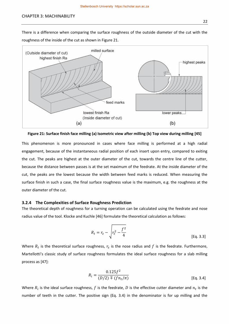
CHAPTER 3: MACHINABILITY 22
There is a difference when comparing the surface roughness of the outside diameter of the cut with the
roughness of the inside of the cut as shown in Figure 21.
Figure 21: Surface finish face milling (a) Isometric view after milling (b) Top view during milling [45]
This phenomenon is more pronounced in cases where face milling is performed at a high radial
engagement, because of the instantaneous radial position of each insert upon entry, compared to exiting
the cut. The peaks are highest at the outer diameter of the cut, towards the centre line of the cutter,
because the distance between passes is at the set maximum of the feedrate. At the inside diameter of the
cut, the peaks are the lowest because the width between feed marks is reduced. When measuring the
surface finish in such a case, the final surface roughness value is the maximum, e.g. the roughness at the
outer diameter of the cut.
3.2.4 The Complexities of Surface Roughness Prediction The theoretical depth of roughness for a turning operation can be calculated using the feedrate and nose
radius value of the tool. Klocke and Kuchle [46] formulate the theoretical calculation as follows:
𝑅𝑡 = 𝑟𝜀 − √𝑟𝜀2 −
𝑓2
4
[Eq. 3.3]
Where 𝑅𝑡 is the theoretical surface roughness, 𝑟𝜀 is the nose radius and 𝑓 is the feedrate. Furthermore,
Martellotti’s classic study of surface roughness formulates the ideal surface roughness for a slab milling
process as [47]:
𝑅𝑖 =0.125𝑓2
(𝐷/2) ∓ (𝑓𝑛𝑡/𝜋)
[Eq. 3.4]
Where 𝑅𝑖 is the ideal surface roughness, 𝑓 is the feedrate, 𝐷 is the effective cutter diameter and 𝑛𝑡 is the
number of teeth in the cutter. The positive sign (Eq. 3.4) in the denominator is for up milling and the
Stellenbosch University https://scholar.sun.ac.za

CHAPTER 3: MACHINABILITY 23
negative sign is for down milling. Mertellotti’s equation assumes that the inserts are spaced perfectly
around the cutter axis and in relation to each other within the cutter body. Additional assumptions relate
to the straightness of the cutter, clamping rigidity, play on the spindle and that the inserts are always sharp.
These conditions are rarely achieved in practice, due to a significant difference between theoretical versus
measured values. Therefore the use of equations 3.3 and 3.4 are limited.
Benardos and Vosniakos [48] produced a review on roughness prediction for machining and validated
previous findings by means of a neural network approach. Findings from reviewed literature point to the
fact that theoretical prediction of surface roughness values is complex, due to a plethora of influencing
factors that should be considered.
Figure 22: Influences on surface quality in metal cutting [46]
Benardos and Vosniakos constructed an intricate fish bone diagram to illustrate the associated
complexities. Similarly, Kloche and Kuchle [46] efficiently summarises the currently known factors that
influence surface quality in metal cutting as shown in Figure 22.
Surface roughness prediction models are known to be limited in their application and scope, because they
are primarily valid for a specific set of conditions [41] [42] [49] [50] [51]. Conversely, Benardos and
Vosniakos conclude that research in the field is increasing and that the resulting contributions are valuable
for development of automated in-line inspection of machining operations.
3.3 CHIP CONTROL
3.3.1 Introduction
Ti-6Al-4V machining generates heat, concentrated at the tool tip, due to the material’s low thermal
conductivity. Chips formed during Ti-6Al-4V machining are characterised by a serrated or segmented
formation, due to the low modulus of elasticity of Ti-6Al-4V. More specifically, the findings Ozel and Sima
[52] suggest that for cutting speeds of 60 m/min and above, serrated chips with accompanying adiabatic
shear bands are visible during electron microscope analysis. Similarly, Komanduri and von Turkovich [53]
Stellenbosch University https://scholar.sun.ac.za

CHAPTER 3: MACHINABILITY 24
report that Ti-6Al-4V is regarded as model material by investigators, because it forms serrated chips at low
cutting speeds. Other materials typically start producing serrated chips at higher cutting speeds.
The physical characteristics of chips provides important evidence about the formation at the shear zone.
The examination of the shape of the chip provides information about the condition of the tool tip, cutting
speed, shear force and temperature at the tool-chip interface.
3.3.2 Chip Classification Criteria
Chips are generally classified into four categories. They are: Continuous chips, segmented or serrated chips,
chips that result from a built-up edge (BUE) on the tool and shearing or discontinuous chips as shown in
Figure 23 [38] [46] [37].
Figure 23: Chip type categories [46]
Continuous chips are formed when ductile materials are machined at high cutting speeds with small
feedrates and ADOC. This type of chip usually produces a desirable surface finish, but tend to tangle around
critical parts of machines such as the tool holder (turning) or cutter body (milling) as well as the fixturing
and chip evacuation system. A continuous chip also provides evidence of low friction at the shear zone,
hence lower cutting temperatures and therefore improved tool life. Chip breakers are frequently used to
control the length of this chip type, that increases the overall manageability thereof. Additional remedies to
control chip geometry include changing cutting speed, ADOC and using cutting fluid [54] [37] [38].
Segmented chips have a distinctive sawtooth appearance due to the cyclical alteration in strain at the shear
zone. This type of chip is also refered to as serrated or non-homogenous. This sawtooth appearance is
characteristic in the machining of difficult-to-cut superalloys, particularly titanium alloys. The sawtooth chip
profile can also be observed with the machining of more common metals at high cutting speeds [54] [37]
[38].
BUE chips are caused by the adherence of the work material to the tool tip due to tool-chip friction at the
shear zone at lower cutting speeds. As the cutting speed increases, the BUE decreases. The magnitude of
the BUE on the tool tip varies constantly as material accumulates on the tip and finally breaks off in a
Stellenbosch University https://scholar.sun.ac.za

CHAPTER 3: MACHINABILITY 25
cyclical manner, until corrective measures are taken. During machining, the BUE material is partially
removed from the tool tip by the in-contact chip area and the rest is deposited on the workpiece surface.
This undesireable effect causes changes in the tool tip geometry and contributes to premature dulling. An
additional drawback is the negative effect of the BUE deposits on the finished workpiece surface. Managing
a smaller BUE is advantegous, because it protects the rake face and extends tool life [54] [38] [37].
Shearing or discontinuous chips are formed when machining a brittle or impure material or during extreme
cutting speeds beyond the machinability guidelines for feedrate and ADOC. Poor workpiece clamping,
flexure in the tool holder and the milling machine are causes of chatter and vibration, that results in
discontinuous chips. Depending on the degree of rigidity in the milling machine setup, the cutting tool may
wear prematurely or even become damaged. The surface finish for ductile materials is negatively impacted
when discontinuous chips are formed, while discontinuous chip formation has a positive impact on surface
finish for less ductile materials such as Ti-6Al-4V. [54] [37] [38]
3.4 TOOL DETERIORATION PHENOMENA Groover [37] lists three failure modes for cutting tools: (1) Fracture failure, (2) temperature failure and, (3)
gradual wear. In agreement to this, the ISO standard for tool life testing in milling defines these three
failure modes as (1) brittle fracture, (2) plastic deformation and, (3) tool wear [55]. These failures can be
subdivided into more specific failure phenomena.
3.4.1 Flank Wear
The typical components of a milling insert for an indexable tool is illustrated in Figure 24. The insert flank
face is represented by A. The flank is the part of the insert that comes into contact with the workpiece as
the cutter rotates. Flank wear results from the friction between the tool flank face and the material being
cut [37]. Friction is high on the flank face and this is where most of the tool wear should occur under
normal Ti-6Al-4V machining conditions. The rake face is the area of the insert that is adjacent to the cutting
edge and denoted by B. The rake face mostly directs the flow direction of the newly cut material. The insert
clamp screw is denoted by D. The insert clamp screw pulls the indexable insert onto the insert seat, which
is represented by C.
Stellenbosch University https://scholar.sun.ac.za

CHAPTER 3: MACHINABILITY 26
Figure 24: Milling insert components
Flank wear is a gradual process and characteristic of normal cutting conditions, however, flank wear can be
accelerated in cases where inadequate lubrication is applied or cutting speeds are excessive [38] [56].
Flank wear is measured by determining the width of the wear bands, also known as the wear land, on the
rake face as shown in Figure 25.
Figure 25: Flank wear measurement criteria for an endmill [57]
The wear land is measured from the position of the original cutting edge even in cases where the edge is
worn away. In such a case, the position of original cutting edge is determined by extending the line from
the neighbouring, unaffected cutting edge. VB 1 is the uniform wear land and usually has a constant width
across the cutting edge. Uniform wear is considered the as the average wear on the cutting edge and
denoted as 𝑉𝑏 in literature. Non-uniform flank wear has an uneven width for all occurrences along the flank
and is illustrated as VB 2 in Figure 25. Non-uniform flank wear is also described as maximum flank wear and
denoted as 𝑉𝑏𝑚𝑎𝑥 in literature. ISO 8688-1 : 1989 [55] further describes localized flank wear as exaggerated
Stellenbosch University https://scholar.sun.ac.za

CHAPTER 3: MACHINABILITY 27
flank wear at localized areas on the flanks. Localized flank wear is referred to as VB 3 and is further
subdivided into notch wear and groove wear as shown in Figure 26.
Figure 26: Localized flank wear in the form of notch wear and groove wear [55]
The flank wear rate can be decelerated by choosing a more suitable tool grade for the material being cut,
reducing cutting speed or selection of a smaller entering angle. The Taylor tool life equation is based on
flank wear:
𝑉𝑇𝑛 = 𝐶 [Eq. 3.5]
Where 𝑉 is the cutting speed, 𝑇 is the time (min) to develop a certain wear land (𝑉𝑏), 𝑛 is a workpiece and
tool material exponent and 𝐶 is a constant. The value for factors 𝑛 and 𝐶 are determined experimentally,
through performing numerous cutting tests at different cutting speeds, feedrates, depths of cut, tool
materials and geometries. Cutting speed is the primary factor affecting tool life [37] [56] [58] [38].
Figure 27: Flank wear as a function of time [58]
The break-in period (Figure 27) sees the tool’s sharp cutting edge rapidly wear during the first few minutes
of machining. During the steady-state wear period, wear is uniform although not a linear relationship over
time in all cases. The failure region marks the useful tool lifetime where cutting temperatures are elevated
and productivity is reduced due to approaching maximum flank wear for the tool [37].
Stellenbosch University https://scholar.sun.ac.za

CHAPTER 3: MACHINABILITY 28
During tool wear experiments, the cutting time is recorded and the wear land is measured. Tool wear
experiments are rather costly, because large amounts of material is removed to record tool wear from
break-in to failure as shown in Figure 27 and also explained earlier in Figure 4 and Figure 8.
Costs are increased for high cost alloys such as Ti-6Al-4V [4]. The cost of recording the tool failure time for
face milling with a tool diameter of 63 mm (Kennametal Beyond Blast KSRM63A04RC20BB) would therefore
not be feasible for academic purposes at university level.
3.4.2 Crater Wear
Crater wear (Figure 28) consists of a concave section on the rake face and occurs with high cutting
temperatures that is caused by chip friction against the rake face. Craters are predominantly measured by
depth or area [38]. Diffusion is usually associated with crater wear. During diffusion, atoms are exchanged
in the tool-chip interface. Diffusion depletes the tool tip of the atoms responsible for its hardness. The tool
then becomes more vulnerable to abrasion and adhesion.
Figure 28: Crater wear [56]
ISO 8688-1 : 1989 [55] also explains how crater wear (KT 1) is typically formed parallel to the major cutting
edge and the maximum crater depth is often located some distance away from the major cutting edge.
Another closely related type of wear is stair-formed face wear (KT 2), in which the maximum depth of the
wear scar occurs at the intersection of the wear scar with the tool major flank.
Figure 29: Stair-formed face wear [55]
Cratering or stair-formed face wear is remedied by reducing the cutting speed and increasing coolant to the
tool-chip interface [37] [56]. ISO 8988-1 : 1989 provides a guideline for maximum crater size in terms of
testing time, under a tool deterioration section [55]. Unfortunately, crater wear can be challenging to
measure accurately.
Stellenbosch University https://scholar.sun.ac.za

CHAPTER 3: MACHINABILITY 29
Figure 30: Vertical scanning interferometer [59]
Devillez, Lesko, and Mozer [59] proposed the use of white light interferometry for the measurement of the
crater depth as shown in Figure 30. During white light interferometry, an optical profiler is used to scan the
object (such as a cratered insert) along the vertical axis. Fringes developed along the crater as each area of
the surface moves into focus. The images are communicated to a computer algorithm that fits the data
with a coherence envelope, which reveals the crater depth.
Alternatively, Hong, Wang, and Wong, [60] measures crater wear by implementing a phase shifting method
to achieve a 3D rendering of the tool surface. During the scanning process, an LCD projects linear sinusoidal
fringe patterns over the insert as shown in Figure 31 (a).
Figure 31: 3D map (b & c) of insert crater (a) [60]
These projections are altered from four different angles with respect to the insert, which is mounted on a
stage in front of the projector and microscope camera. The images are captured by a long working distance
microscope. The captures 256-graylevel images are then processed to map the 3D surface as shown in
Figure 31 (b & c).
3.4.3 Notch and Groove Wear
Notch and groove wear is characterised by a noticeable indentation at a certain point along the worn major
and minor flank face. ISO 8988-1 : 1989 [55] categorises notch and groove wear under localized flank wear,
because the notches develop on the area of the major flank adjacent to the work surface during cutting as
Stellenbosch University https://scholar.sun.ac.za

CHAPTER 3: MACHINABILITY 30
shown in Figure 32 b. However, groove wear is formed on the area of the minor flank adjacent to the
machined surface during cutting as shown in Figure 32 a.
Figure 32: (a) Groove wear, (b) Notch wear [56]
Notches or grooves are initiated when machining a material that has an inconsistent hardness gradient. In
practice a hardened outer layer is encountered. Residues from sand casting, hardening from cold drawing
or previous machining are the main causes of notch wear. Sandvik Coromant [56] suggests that notch or
groove wear can be caused by excessive cutting speed and Kennametal blames incorrect cutter geometry
[45].
3.4.4 Plastic Deformation Plastic deformation (PD) is the distortion of the cutting part of a tool from its original shape without initial
loss of tool material as shown in Figure 33 [55]. During PD, the cutting tool edge geometry is transformed
by high temperatures at the tool-chip interface. The cutting force pressure on the tool further contributes
to the deformation of the geometry.
Figure 33: Plastic deformation [56]
A plastically deformed tool is more susceptible to flank wear, because of increased abrasion. PD is reduced
by selecting a harder grade tool, reducing feedrate and cutting at a lower speed [56].
3.4.5 Chipping
Chipping patterns have a saw-toothed appearance and can easily be mistaken for normal flank wear as
shown in Figure 34. An ineffectively clamped workpiece or re-cutting of chips is often the cause [45] [56].
Stellenbosch University https://scholar.sun.ac.za

CHAPTER 3: MACHINABILITY 31
Figure 34: Non-uniform chipping (CH 2) [56]
There are four types of chipping according to ISO 8988-1 : 1989: (CH 1) Uniform chipping, where the loss of
tool fragments along the cutting edge is around the identical size, (CH 2) Non-uniform chipping which is
formed at a few positions along the active cutting edges but with no uniformity from one cutting edge to
another, (CH 3) Localized chipping which happens consistently along specific locations along the active
cutting edge, and (CH 4) Chipping of the non-active part of the major cutting edge, which is formed outside
the active part of the cutting edge due to chip hammering [55].
Chipping can be reduced by changing from a tool with a neutral geometry to a lead angle geometry. Rigid
clamping reduces chatter and an increase in coolant pressure or better delivery system helps to prevent the
re-cutting of chips [56] [45].
3.4.6 Edge Fracture or Catastrophic Failure This phenomenon (Figure 35) is observed when there is rapid deterioration to complete failure of the
cutting part [55]. A number of factors contribute to edge fracture: Excessive load on the insert, BUE,
excessive tool wear, tool grade and incorrect geometry [56]. Edge fracture can also occur in cases similar to
chipping, due to lack of stability in the workpiece clamping.
Figure 35: Edge fracture [56]
Edge fracture can be reduced by reducing the feedrate and ADOC, while ensuring that the workpiece is
rigidly clamped. Selection of a more suitable insert type, with regards to geometry and grade reduces the
chances of fractures.
3.4.7 Thermal Cracking
Thermal cracking is induced by extreme temperature variations within the cutting tool insert during cutting.
There are three types of cracks: (CR 1) Comb cracks which form on the tool face and the tool flank and are
oriented perpendicular to the major cutting edge, (CR 2) Parallel cracks that appear on the tool face or the
Stellenbosch University https://scholar.sun.ac.za
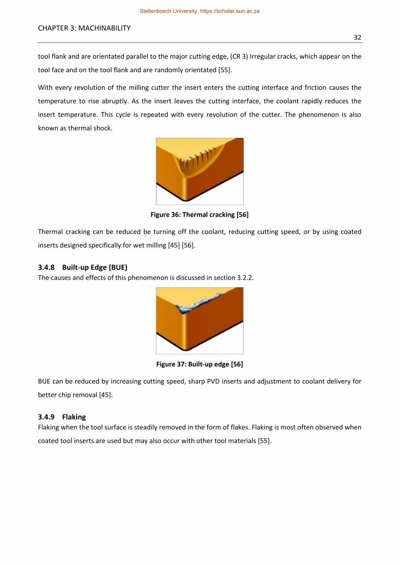
CHAPTER 3: MACHINABILITY 32
tool flank and are orientated parallel to the major cutting edge, (CR 3) Irregular cracks, which appear on the
tool face and on the tool flank and are randomly orientated [55].
With every revolution of the milling cutter the insert enters the cutting interface and friction causes the
temperature to rise abruptly. As the insert leaves the cutting interface, the coolant rapidly reduces the
insert temperature. This cycle is repeated with every revolution of the cutter. The phenomenon is also
known as thermal shock.
Figure 36: Thermal cracking [56]
Thermal cracking can be reduced be turning off the coolant, reducing cutting speed, or by using coated
inserts designed specifically for wet milling [45] [56].
3.4.8 Built-up Edge (BUE)
The causes and effects of this phenomenon is discussed in section 3.2.2.
Figure 37: Built-up edge [56]
BUE can be reduced by increasing cutting speed, sharp PVD inserts and adjustment to coolant delivery for
better chip removal [45].
3.4.9 Flaking Flaking when the tool surface is steadily removed in the form of flakes. Flaking is most often observed when
coated tool inserts are used but may also occur with other tool materials [55].
Stellenbosch University https://scholar.sun.ac.za

CHAPTER 3: MACHINABILITY 33
Figure 38: Flaking on the cutting edge of a turning insert [61]
Flaking can also be caused in cases where the cutting tool is used at feedrates or cutting speeds in excess of
the tool manufacturer’s specifications for that particular material [62].
3.5 FORCE AND POWER REQUIRED
3.5.1 Forces in Machining Knowledge of the magnitude of the cutting forces during machining is important. Kalpakjian et al. [38]
elaborates on the significance of cutting force data: The design of machine tools is based on the magnitude
of cutting forces, amongst other factors. A knowledge of the cutting forces prevents distortion of machine
components, maintains the desired dimensional accuracy of the machined part and aids in selecting correct
tool and work holding devices. Attention to these factors reduces the distortion of the finished workpiece.
The power requirements also need to be determined for selection of the appropriate machine tool.
A cutting force diagram can be constructed to determine the force components acting on the tool and
workpiece as shown in Figure 39 [46]. This force diagram is known as a Merchant force diagram and is
named after its creator, Eugene Merchant [63]. Merchant’s force wheel is interpreted as follows: In Figure
39, the forces acting on the chip are divided into two perpendicular components, namely friction force (𝐹𝛾)
and normal force to friction (𝐹𝛾𝑛). 𝐹𝛾𝑛 is perpendicular to 𝐹𝛾. These two forces are used to define the
coefficient of friction between the tool and chip:
𝜇 =𝐹𝛾
𝐹𝛾𝑛
[Eq. 3.6]
The vectors 𝐹𝛾 and 𝐹𝛾𝑛 are added to form the resultant force 𝐹𝑧 which is orientated at angle 𝜌. This angle is
known as the friction angle [37]. The relationship of the friction angle (𝜌) and the coefficient of friction is
written as:
𝜇 = tan 𝜌 [Eq. 3.7]
There are also two additional tool forces components acting on the chip, namely shear force (𝐹𝜙) and
normal force to shear (𝐹𝜙𝑛). Shear force (𝐹𝜙) causes shear deformation at the shear plane to which the
Stellenbosch University https://scholar.sun.ac.za
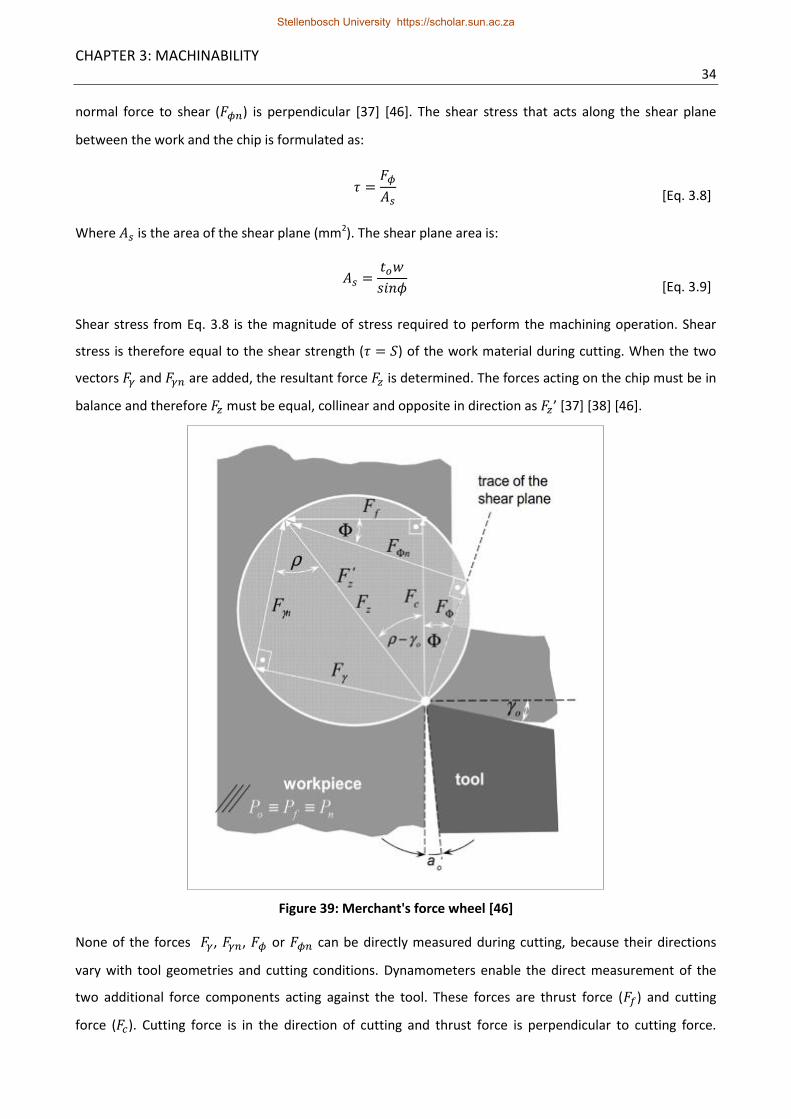
CHAPTER 3: MACHINABILITY 34
normal force to shear (𝐹𝜙𝑛) is perpendicular [37] [46]. The shear stress that acts along the shear plane
between the work and the chip is formulated as:
𝜏 =𝐹𝜙
𝐴𝑠
[Eq. 3.8]
Where 𝐴𝑠 is the area of the shear plane (mm2). The shear plane area is:
𝐴𝑠 =𝑡𝑜𝑤
𝑠𝑖𝑛𝜙
[Eq. 3.9]
Shear stress from Eq. 3.8 is the magnitude of stress required to perform the machining operation. Shear
stress is therefore equal to the shear strength (𝜏 = 𝑆) of the work material during cutting. When the two
vectors 𝐹𝛾 and 𝐹𝛾𝑛 are added, the resultant force 𝐹𝑧 is determined. The forces acting on the chip must be in
balance and therefore 𝐹𝑧 must be equal, collinear and opposite in direction as 𝐹𝑧’ [37] [38] [46].
Figure 39: Merchant's force wheel [46]
None of the forces 𝐹𝛾, 𝐹𝛾𝑛, 𝐹𝜙 or 𝐹𝜙𝑛 can be directly measured during cutting, because their directions
vary with tool geometries and cutting conditions. Dynamometers enable the direct measurement of the
two additional force components acting against the tool. These forces are thrust force (𝐹𝑓) and cutting
force (𝐹𝑐). Cutting force is in the direction of cutting and thrust force is perpendicular to cutting force.
Stellenbosch University https://scholar.sun.ac.za
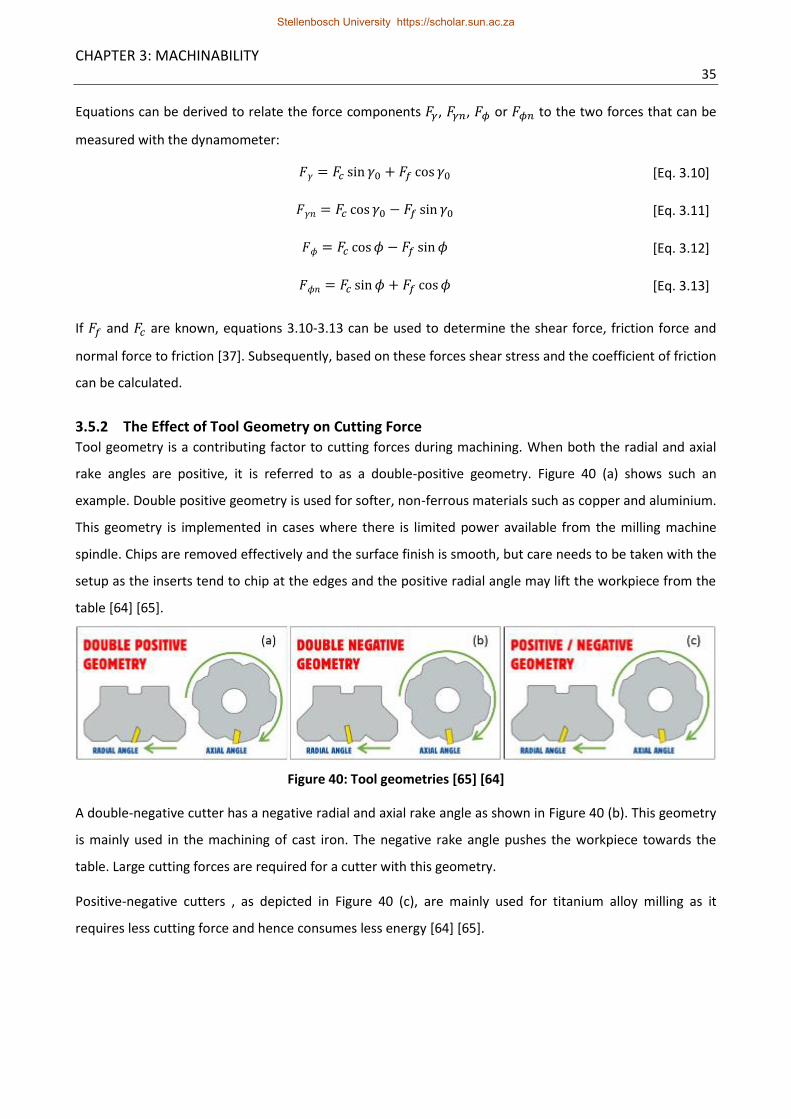
CHAPTER 3: MACHINABILITY 35
Equations can be derived to relate the force components 𝐹𝛾, 𝐹𝛾𝑛, 𝐹𝜙 or 𝐹𝜙𝑛 to the two forces that can be
measured with the dynamometer:
𝐹𝛾 = 𝐹𝑐 sin 𝛾0 + 𝐹𝑓 cos 𝛾0 [Eq. 3.10]
𝐹𝛾𝑛 = 𝐹𝑐 cos 𝛾0 − 𝐹𝑓 sin 𝛾0 [Eq. 3.11]
𝐹𝜙 = 𝐹𝑐 cos 𝜙 − 𝐹𝑓 sin 𝜙 [Eq. 3.12]
𝐹𝜙𝑛 = 𝐹𝑐 sin 𝜙 + 𝐹𝑓 cos 𝜙 [Eq. 3.13]
If 𝐹𝑓 and 𝐹𝑐 are known, equations 3.10-3.13 can be used to determine the shear force, friction force and
normal force to friction [37]. Subsequently, based on these forces shear stress and the coefficient of friction
can be calculated.
3.5.2 The Effect of Tool Geometry on Cutting Force
Tool geometry is a contributing factor to cutting forces during machining. When both the radial and axial
rake angles are positive, it is referred to as a double-positive geometry. Figure 40 (a) shows such an
example. Double positive geometry is used for softer, non-ferrous materials such as copper and aluminium.
This geometry is implemented in cases where there is limited power available from the milling machine
spindle. Chips are removed effectively and the surface finish is smooth, but care needs to be taken with the
setup as the inserts tend to chip at the edges and the positive radial angle may lift the workpiece from the
table [64] [65].
Figure 40: Tool geometries [65] [64]
A double-negative cutter has a negative radial and axial rake angle as shown in Figure 40 (b). This geometry
is mainly used in the machining of cast iron. The negative rake angle pushes the workpiece towards the
table. Large cutting forces are required for a cutter with this geometry.
Positive-negative cutters , as depicted in Figure 40 (c), are mainly used for titanium alloy milling as it
requires less cutting force and hence consumes less energy [64] [65].
Stellenbosch University https://scholar.sun.ac.za

CHAPTER 3: MACHINABILITY 36
3.5.3 Power Required in Machining
Cutting power is the product of force and velocity. The cutting power is largely dissipated in the shear zone
(due to energy required to shear the material) and at the rake face of the tool (due to tool-chip interface
friction) [38].
The power equation can therefore by derived as [45] [37] [38]:
𝑃𝑠 = 𝐹𝑐𝑣𝑐 [Eq. 3.14]
Where 𝑃𝑠 = power at spindle (kW), 𝐹𝑐 is the cutting force component and 𝑣𝑐 is the cutting speed. The
instantaneous power required by a certain cut is limited by the maximum allowable power at any given
revolutions per minute according to the milling machine spindle specification for power and torque
delivery.
3.5.4 Modeling of Cutting Forces A significant amount of publications cover the area of modeling cutting forces for a machining operation.
Most popular among these are models for drilling, milling and turning operations. Publications also differ in
their modeling approach: Some follow a mechanistic approach to predict cutting forces, while others rely
on the finite element method (FEM). In addition, the statistical or nonparametric approach to force
prediction is increasingly used. The statistical approach differs from mechanistic and FEM approaches in
that the majority of experiments for such a model are performed before modeling is done. Thereafter it is
commonplace to utilise tools such as analysis of variance (ANOVA) or regression to evaluate factorial
relationships and also test the error between the model and experimental values. The inverse is true for
mechanistic and FEM modeling.
During the classic study of Chandrasekharan, DeVor, and Kapoor, [66] a mechanistic model was developed
from first principles to predict thrust force during drilling. The mechanistic model was compared to
experiment results and a maximum error of 10% was reported in the predicted mean thrust values.
Similarly, Baro, Joshi, and Kapoor [67] developed a mechanistic model for face milling. The purpose of the
model is to predict cutting forces for face milling with self-propelled round inserts. Baro et al. follows the
same methodology as Chandrasekharan et al. in that a mechanistic model is validated with experiments.
Additional factors considered by Baro et al. are the various frictions acting on the cutting interface,
geometry of the insert and geometry of the cutter. Experiments are validated using a dynamometer. The
maximum error between measured and predicted forces is 17% for this study.
Another mechanistic prediction model is that of Huang and Liang [68]. They derived a mechanistic force
prediction model for turning, considering the tool wear effect. Subsequently, a genetic algorithm was
applied to identify the coefficients, due to the absence of explicit normal equations. Finally, cutting force
Stellenbosch University https://scholar.sun.ac.za

CHAPTER 3: MACHINABILITY 37
prediction was validated through obtaining experiment results by means of a dynamometer mounted to
the tool post.
Hsieh, Shih, and Strenkowski [69] modeled drilling thrust force with a FEM technique. The model was
validated with laboratory experiments at several drill diameters, spindle speeds and feedrates.
Furthermore, Altan and Özel [70] developed a FEM model for flat end milling, which was then validated
with experiments, using a dynamometer. Experimental results showed “reasonable agreement” with
predicted force values. The interpretation of the results follow a subjective approach due to the prediction
of an entire cut cycle waveform instead of a mean force value for a given axis. The predicted values appear
to closely follow the maximum measured cutting force along the force curve.
The FEM approach taken by Hossan and Qian [71] for predicting cutting force during a turning operation
differs slightly from other modeling approaches as it uses results from literature to validate predicted
values. Predicted force error is a maximum of 15% when compared to results from literature. It is worth
mentioning that models are often validated against results from literature if researchers do not have access
to high cost testing equipment such as dynamometers or heavy milling machines.
Hocheng and Tsao [72] follows the Taguchi method: Multi-variable linear regression through ANOVA to
statistically predict thrust forces during core drilling of carbon fibre reinforced polymer. The correlation
between thrust force and cutting parameters is also described. Verification of the predictive model reveals
a maximum error of 15.3%.
Amin, Faris, and Patwari (2009) [73] incorporates experimental design and (response surface methodology)
RSM to predict tangential cutting force in end milling. The cutting parameters of the model are ADOC,
feedrate and cutting speed. The measured response is tangential cutting force. Through ANOVA it was
determined that the cutting force is most affected by feedrate, then ADOC, and finally cutting speed.
Central composite design was applied to develop the force model in relation to the cutting parameters. The
significance of the model was verified with ANOVA at a 95% confidence level.
During turning experiments Bouacha, Mabrouki, Rigal, and Yallese [74] explores the relationship between
machining input parameters and output variables with RSM. The effect of ADOC, feedrate and cutting
speed on cutting force is determined through ANOVA. Bouacha et al. finds that the ADOC has the largest
influence on the cutting forces measured during experimentation.
3.5.5 Response Surface Methodology (RSM) Montgomery [75] [76] defines RSM as, “A collection of mathematical and statistical techniques useful for
the modeling and analysis of problems in which a response of interest is influenced by several variables and
the objective is to optimize this response.” RSM is a sequential technique for following a path to the
Stellenbosch University https://scholar.sun.ac.za

CHAPTER 3: MACHINABILITY 38
optimum response surface. The path that the experimenter follows is called the method of steepest ascent,
and in cases where minimization is required, it is called the method of steepest descent.
Figure 41: The sequential nature of RSM [75]
The response surface can be represented by the entire curved surface in Figure 41. The relationship
between the dependent and the independent variables is often unknown at first. The experimenter usually
starts some distance away from the optimum as shown by the ‘current operating conditions’ in Figure 41.
First, the experimenter needs to approximate the true functional relationship between the response and
the independent variables employed. This is usually achieved through a first-order model that is derived
from a fractional factorial or full factorial design as shown in Figure 42 (a) and (b) respectively. If the
response is well modeled by a linear function of the independent variables, then the approximating
function is the first-order model. If this is not the case, then the steepest ascent method is followed until a
decrease in response is observed as shown by the contours in Figure 41 [75] [77].
Figure 42: (a) Fractional factorial (b) Full factorial with centre points (c) Central composite design
A factorial design with centre points, as shown in Figure 42 (b), is then fitted around this region. If the
ANOVA for this model reveals no significant curvature, then a first-order model may very well adequately
represent the optimum surface. Conversely, if significant curvature is detected by the full factorial design,
then additional experiments need to be performed to establish a second-order model [75] [78]. A second-
order model usually significantly describes the response surface, but in certain cases a third or fourth-order
Stellenbosch University https://scholar.sun.ac.za

CHAPTER 3: MACHINABILITY 39
model might be of better significance. Additional experimentation usually follows a central composite
design methodology as illustrated in Figure 42 (c).
The second-order model fitted by means of the central composite design method allows the experimenter
to construct a response surface with the aid of computer software.
Figure 43: Contours and response surface [76]
RSM is a valuable tool in determining the optimum operating characteristics of the modeled function,
especially when a rotatable design was chosen. Figure 43 shows the concentric circle contours, which
means that the response is the same on all points along the same contour that are the same distance from
the centre of the design. The valley represented by the 3-dimensional response surface in Figure 43 further
shows that the optimum response values are for a minimization problem and that a method of steepest
descent was followed. The response values around the centre contours are therefore minimum optima.
3.6 CONCLUSION AND REMARKS
Surface finish is generally measured with a profilometer in micron and the arithmetic mean surface
roughness method is followed. Surface roughness is affected by numerous factors that are difficult to
control in practice. Despite the widespread use of the arithmetic mean surface roughness method, there
are limitations to its accuracy.
Conditions at the tool-chip interface affect chip formation. There are four main categories for the types of
chips. Furthermore, the characteristics of machined chips provide evidence about machinability factors
such as the material being cut, the magnitude of the cutting force, geometric features of the cutting tool
and the quality of surface finish and integrity. Chip analysis is an important tool in the improvement of
machining operations.
Tool wear is a factor of productivity and is typically affected by cutting speed. There are roughly nine
different categories of tool wear. The type of tool wear observed during a machining operation suggests
the specific corrective measures that needs to be taken for increased productivity. Flank wear is the
principal measure of tool wear and tools normally wear according to three distinct phases over time. Tool
Stellenbosch University https://scholar.sun.ac.za
CHAPTER 3: MACHINABILITY 40
wear is measured by recording the width of the wear land on the insert flank. Tool wear measurement
requires microscopy. Examination of tool wear across all three phases of wear can be a time consuming and
therefore costly exercise, depending on the amount and the cost of the material that will be removed
during the experiment.
Milling machines and tools are designed according to the type of forces present at the tool-chip interface.
The cutting force component is measured in the direction of the cutting speed and is used to determine the
required force for the cutting operation. Although the magnitude and direction of all force components
during cutting cannot be theoretically determined, dynamometers enable the measurement of thrust force
and cutting force. Equations 3.10 to 3.13 allow the determination of friction force, normal force to friction,
shear force and normal force to shear in cases where the cutting force and thrust force is known.
Modeling of cutting forces for drilling, milling and turning is a popular subject for researchers. Past papers
provide ample groundwork to build on in terms of methodology when modeling. There are three types of
approaches mainly used for cutting force modeling: Mechanistic, FEM and statistical. When taking into
consideration an industrial engineering approach to answer the research questions of this thesis, it
becomes apparent that the statistical methods discussed in this chapter offer a more suitable way forward
in terms of modeling.
The literature review reveals that a reasonable amount of papers follow the response surface
methodology. RSM provides an iterative sequence of arriving at an optimum solution for modeling a
particular response surface and subsequently fitting a first, second, third or even fourth-order model of
significance. The RSM technique in its entirety can become a lengthy process in terms of the number of
experiments that are required to accurately model a specific response surface. The reason therefore is
within the sequential experimental approach that needs to be followed before and after the application of
the steepest ascent method. A well prepared full factorial design with centre points can provide
information about the location of the optimum surface area by examining the curvature represented in the
location of the central points.
Stellenbosch University https://scholar.sun.ac.za

CHAPTER 4: METHODOLOGY 41
CHAPTER 4
METHODOLOGY
4.1 INTRODUCTION The experimental design is tailored to provide conclusive results for Ti-6Al-4V cutting experiments. The
overall goal of the experiments is to: (1) Measure and inspect tool wear, chip formation, surface finish and
tangential cutting forces, (2) Fit a statistical model to the experimental data for the purpose of cutting force
prediction.
4.2 PREPARATION OF MATERIAL, TOOLS AND EQUIPMENT The experimental design follows procedures set forth by ISO 8688-1 [55] and 8688-2 [57]. These guidelines
are aimed at experimentation with end milling and face milling respectively. Important experimental design
factors for consideration include: (1) Workpiece material properties, (2) Tool geometry and cutting edges,
(3) Cutting fluid and lubricant, (4) Cutting strategy, (5) Tools and tool holders, and (6) Machine tool.
4.2.1 Workpiece Material The workpiece material used for experiments is Ti-6Al-4V, grade 5. The required properties and
specifications of the Ti-6Al-4V bar used for experiments are listed in Table 4.
Table 4: Workpiece material properties
Material Ti-6Al-4V
Supplier Sierra Alloys
Product Code MIL T-90451
Grade 5
Condition Annealed
Vickers Hardness (HV) 342.3
Rockwell Hardness (HRC) 34.7
Tensile Strength (N/mm2) 1100.25
Chemical Composition Al (6%) – Fe (0.25%) – O (0.2%) – Ti (90%) – V (4%)
Final Dimensions (W x L x H) 101.68 mm x 73.20 mm x 92.3 mm
The surface scale on the Ti-6Al-4V bar was removed prior to milling experiments. The hardness of the
material was verified to confirm the information provided by the product data sheet. The testing zone
Hardness testing was performed at five points along the centre line of the test zone or width of cut area as
shown in Figure 44.
Hardness readings were taken on the testing zone before and after experiments, to check the hardness
gradient throughout the workpiece. The average Vickers hardness of the uncut testing section was 342 HV
and the average hardness of the cut section was 342.6 HV. The width of the cut is 43 mm. The marking out
of the hardness testing points along the experimental area on the Ti-6al-4V sample is shown in Figure 44.
Stellenbosch University https://scholar.sun.ac.za

CHAPTER 4: METHODOLOGY 42
Figure 44: Material hardness testing procedure [55]
4.2.2 Tool Geometry and Cutting Edges The Kennametal KSRM63A04RC20BB cutter body and RCGX2006M0SGF inserts as shown in Figure 45 is
used for cutting experiments. The cutter is designed for machining with Ti-6Al-4V. Due to the large tool
diameter and 20mm inserts, this tool is capable of high material removal rates at higher radial engagement.
Figure 45: Kennametal KSRM63A04RC20BB cutter geometry
The cutter has a neutral axial rake angle and neutral radial rake angle as shown in Figure 45. A neutral
geometry is uncommon for a Ti-6Al-4V face milling cutters. In cases where a cutter has a positive axial rake
angle, it usually ranges between 5° to 20° (positive) for Ti-6Al-4V purposes. Similarly, the radial rake angle
ranges from 1° to 14° [79]. Kennametal developed the KSRM63A04RC20BB cutter body for through spindle
cooling with split tools. This is achieved by channelling the coolant through the cutter body and out through
the insert rake face as shown in Figure 46.
Figure 46: Insert coolant channel alignment with cutter body
Stellenbosch University https://scholar.sun.ac.za

CHAPTER 4: METHODOLOGY 43
The RCGX insert range is manufactured from carbide and the RCGX2006M0SGF inserts have a TiAlN coating
which is applied by means of the Physical Vapour Deposition (PVD) process [80]. TiAlN is the next derivative
coating of titanium nitride (TiN).
Horling, Hultman, Karlsson, Larsson, Mayrhofer, Mitterer, and Sjolen, found that TiAlN outperforms TiN
coatings in high speed machining applications, because TiAlN coatings undergo “spinodal decomposition”,
that hardens the insert at elevated temperatures. Furthermore it was determined that TiAlN has higher
resistance against oxidation due to the formation of an aluminium-oxide layer [81].
Figure 47: RCGX2006M0SGF insert [82]
The RCGX2006M0SGF insert is designed for heavy Ti-6Al-4V milling, hence its larger nose radius. These
inserts each have six indexable positions with an anti-rotation notch in the cutter body. RCGX2006M0SGF
inserts have a 0° rake angle and 7° relief angle [80] [82].
4.2.3 Milling Machine Face milling experiments were conducted on a Hermle C40 milling machine in the Rapid Product
Development Laboratory. The milling machine configuration for the experiments is summarized in Table 5.
Table 5: Milling machine configuration
Machine Tool Hermle C40
Spindle HSK A 63 (18 000 rpm/130 Nm/15 kW)
Coolant Blaser Vasco 5000 (Diluted to 12% concentration)
Coolant Delivery Through spindle, through insert (split tooling)
Coolant Pressure 65 Bar
Cutter Kennametal KSRM63A04RC20BB
Inserts Kennametal RCGX2006M0SGF
Radial Engagement 43 mm
Cutting Force Measurement Kistler 9255C Dynamometer
The tangential cutting force was measured with a Kistler dynamometer attached between the Hermle C40
bed and the workpiece. A force signal cable connects the dynamometer and charge amplifier, which is
connected to the data acquisition system (DAQ). The magnitude and direction of the cutting force
Stellenbosch University https://scholar.sun.ac.za

CHAPTER 4: METHODOLOGY 44
components are then communicated from the DAQ to the Dynoware software by USB interface. The force
measurement system is summarised in Figure 48.
Figure 48: Force measurement experiment setup
The arithmetic mean surface roughness of the outside and inside diameter of each cut was measured with
a Mitutoyo SJ-201P profilometer. The surface finish was measured after each run, because every successive
cut creates its own surface finish, removing the previous surface. The average of three readings was taken
on each side of the cut. The surface roughness of the inside diameter of the cut was labelled as Ra1 and the
roughness of the outside diameter of the cut was labelled as Ra2.
The indexing of inserts after each experiment run enabled measurement of tool flank wear. Each insert has
six indexable positions and each position was marked with a scriber. The marking of inserts followed an
alpha numeric convention: Insert number, followed by the index position according to the alphabet. Insert
three at index B would be labelled as 3B for example. Uniform tool wear measurements were made at six
intervals along each insert’s indexed flank and the average was measured with an Olympus GX51
microscope.
Machining chips were collected for analysis after each experiment run. The milling machine’s table was
cleaned with a high pressure nozzle after every experiment run, to prevent mixing of chips. The chips were
stored in labelled plastic containers for microscope analysis. Chip formation and characteristics were
examined with an Olympus SZX7 Zoom Stereo microscope.
4.2.4 Cutting Strategy Straight cuts were performed for experiments. Each successive straight line cut was made on top of the
previous cut. The radial engagement of 43 mm remained constant for all experiments as the cutting speed,
ADOC and feedrate were varied according to the experimental design matrix. The cutter was not rolled into
Stellenbosch University https://scholar.sun.ac.za

CHAPTER 4: METHODOLOGY 45
cuts, hence thicker initial chips can be expected. The down milling technique, popular with Ti-6Al-4V
milling, was used as described by Tschätsch and Reichelt [83].
4.3 EXPERIMENTAL DESIGN
4.3.1 Introduction
The pre-experimental planning was done by means of constructing a fish bone diagram of controllable,
uncontrollable and constant factors. These factors are illustrated in Figure 49.
Figure 49: Experiment design factors
The choice of experimental design is determined by the desired sample size [75]. In this case, the high price
and limited availability of Ti-6Al-4V in South Africa requires a small sample size. A full factorial design with
three variables at two levels and three centre points (23+3) was chosen. This particular design was chosen,
because it is the most efficient design for the study of two or more factors [75] [84]. The addition of centre
points to the full factorial design enables curvature testing. This provides an indication of how far the
selected response surface is from a change in the sign of the gradient, indicating a possible optimum [75]
[76] [85] [77] [78].
4.3.2 Research Hypothesis
If both the curvature and lack of fit is not significant, while the model is found to be significant, then a first-
order model accurately represents the optimal response surface of tangential cutting forces. On the other
hand, if there is significant curvature, the first-order model, despite being fitted significantly to the current
response surface, does not represent the optimum response surface [75] [85]. Therefore the following
hypothesis can be derived:
H0 : A first-order model significantly represents the optimal response surface of tangential cutting forces.
Stellenbosch University https://scholar.sun.ac.za

CHAPTER 4: METHODOLOGY 46
H1 : A first-order model represents a response surface different from the optimum of tangential cutting
forces.
4.3.3 Research Methodology for Statistical Modeling The chosen methodology follows the steps shown in Figure 50. Response surface methodology (RSM)
cannot be followed in its entirety due to the amount of experiments required to determine the optimum
response surface by means of the steepest ascent method. The methodology provides a best model fit
solution for the given design space by means of systematic increase of the model order if a better fit is
required.
Estimate sums of squares and mean
squares
Determine effect contributions
Hypothesis test: Significance of
Curvature
Construct initial ANOVA table
Examine significance of
terms, drop insignificant terms
Create reduced model and
perform ANOVA
Hypothesis test: Significance of reduced model
Diagnostic plots and graphs
Interpret results
Hypothesis test: �Lack-of-fit
Improvement Needed? NO
Estimate sums of squares and mean
squares
YES
First Order Model Fitting
Raise Model Order
Hypothesis test: Significance of
model and �Lack of Fit
Inspect tool wear, chips, cutting
force and surface finish
Perform Ti-6Al-4V cutting
experiments
Coding of Ti-6Al-4V experiments
Data Collection
Negative tool wear effects?
NOYES
Figure 50: Research methodology
Stellenbosch University https://scholar.sun.ac.za

CHAPTER 4: METHODOLOGY 47
4.3.4 Coding of Experimental Matrix
The variables chosen for experimentation are feed per tooth (𝑓𝑧), ADOC (𝑎𝑝) and cutting speed (𝑣𝑐). The
measured response is tangential cutting force (𝐹𝑥). Using orthogonal coding, the low and high levels of the
factors are listed for eight runs as shown in Table 6. The addition of centre points to the factorial design,
allows an independent estimate of error to be calculated [75].
Table 6: Coding of the design matrix.
CODED FACTORS Effect Labels
FACTOR LEVELS
Run A (𝒂𝒑) B (𝒇𝒛) C (𝒗𝒄) Factor Low (-) High (+) Centre
(0)
1 ̶− ̶− ̶− (1) A (𝑎𝑝 mm) 0.50 2.50 1.50
2 + ̶− ̶− a B (𝑓𝑧 mm) 0.05 0.15 0.10
3 ̶− + ̶− b C (𝑣𝑐 m/min) 55.00 99.29 77.15
4 + + ̶− ab
5 ̶− ̶− + c
6 + ̶− + ac
7 ̶− + + bc
8 + + + abc
9 0 0 0 Centre
10 0 0 0 Centre
11 0 0 0 centre
4.3.5 Cutting Experiment Worksheet The experimental design run chart, as shown in Table 7, was developed using the Design Expert 7 software
package from Stat-Ease. Values under the heading “Exp.” is the order from 1 to 11 in which experiments
were performed. The “Run” order follows the standard full factorial (23+3) design matrix according to Table
6.
Table 7: Experimental design run chart
Factors Effect
Exp. Run A (𝒂𝒑) B (𝒇𝒛) C (𝒗𝒄) Labels
10 1 0.50 0.05 55.00 (1)
3 2 2.50 0.05 55.00 a
1 3 0.50 0.15 55.00 b
2 4 2.50 0.15 55.00 ab
6 5 0.50 0.05 99.29 c
9 6 2.50 0.05 99.29 ac
4 7 0.50 0.15 99.29 bc
5 8 2.50 0.15 99.29 abc
7 9 1.50 0.10 77.15 Centre
11 10 1.50 0.10 77.15 Centre
8 11 1.50 0.10 77.15 Centre
Stellenbosch University https://scholar.sun.ac.za

CHAPTER 4: METHODOLOGY 48
The tangential cutting forces are recorded for each experiment. Analysis of the machinability factors
determines if the measured forces are acceptable for modeling purposes. If the machinability analysis
provides evidence of catastrophic tool failures, high temperatures or abnormal chip formation, then the
recorded cutting forces are rejected and adjustments need to be made to the face milling experimental
design run chart. If no problems are observed during the machining of the Ti-6Al-4V, then the tangential
cutting force data is useful for the purpose of statistical modeling.
Stellenbosch University https://scholar.sun.ac.za

CHAPTER : EXPERIMENTAL RESULTS AND STATISTICAL MODELING 49
CHAPTER 5
EXPERIMENTAL RESULTS AND STATISTICAL MODELING
5.1 SURFACE FINISH Ra1 is lowest at high ADOC, high cutting speed and low feedrate as shown in Figure 51. Alternatively Ra1 is
highest at medium ADOC, medium cutting speed and medium-to-high feedrate. Figure 51 shows
agreement with findings from the literature review: surface roughness is primarily affected by feedrate.
Figure 51: Surface roughness measured on inside diameter of cut (Ra1)
The measured surface roughness on the outside diameter (Ra2) also suggests feedrate as a primary
affecting factor as shown in Figure 52. The surface roughness is greatest with high-to-medium feedrates
and surface roughness is lower with smaller feedrates. It is also observed that high ADOC increases surface
roughness along with higher feedrates. The maximum recorded surface roughness is 1.26 μm as shown in
Figure 52, while the minimum recorded surface roughness was 0.2 μm as shown in Figure 51.
Figure 52: Surface roughness measured on outside diameter of cut (Ra2)
Stellenbosch University https://scholar.sun.ac.za

CHAPTER : EXPERIMENTAL RESULTS AND STATISTICAL MODELING 50
The recorded data for surface roughness confirms that the Kennametal KSRM63A04RC20BB cutter with
RCGX2006M0SGF inserts is able to perform semi finishing and finishing of machined surfaces. Typical
surface finish for components manufactured by the Daliff Engineering industry partner ranges from 1.6 μm
to 3 μm.
5.2 TOOL WEAR Uniform tool wear measurements were made at six intervals along each insert’s indexed flank and the
average was recorded as shown in Figure 54.
Figure 53: Experiment run 2, Insert 3, index B: Six uniform wear measurements along flank (at 100 μm)
Cutting experiment duration ranged from 18 seconds to 97 seconds, which represents the tool break-in
period as discussed in section 3.4.1 and illustrated in Figure 27. Therefore, the data recorded for the
purpose of tool wear examination cannot be used to model tool wear rate prediction. However the
microscope analysis of the insert flanks is required to assess if tangential cutting force measurements were
conducted under ideal or normal conditions. If there were to be chatter or heat induced tool failures, the
accuracy of the tangential cutting force measurement data becomes questionable.
Examination of the flank wear types gives an indication of conditions at the cutting interface. Uniform flank
wear was observed during all 11 runs. Non uniform flank wear was also observed in four separate runs, but
in negligible magnitudes of 5 μm to 10 μm in the worst cases. These observations were therefore omitted
from results. Figure 54 shows that tool wear rate is affected by the cutting variables ADOC, feedrate and
cutting speed.
Stellenbosch University https://scholar.sun.ac.za

CHAPTER : EXPERIMENTAL RESULTS AND STATISTICAL MODELING 51
Figure 54: Average tool wear for experimental runs
The average uniform tool wear graph (Figure 54) shows that maximum tool wear rate was observed at high
levels for feedrate, ADOC and cutting speed. Conversely, the lowest tool wear rate was observed at low
feedrate, low ADOC and low cutting speed. The microscope analysis therefore concludes that cutting
conditions were normal and tangential force measurements are accurate enough to perform modeling of
the data.
Figure 55: Material removal rate per experimental run
The MRR’s for experiments are shown in Figure 55. The highest MRR of 36.25 cm3/min is in agreement
with Kennametal’s marketed MRR for Beyond Blast cutters.
5.3 CHIP CONTROL AND CHARACTERISTICS Serrated chips were observed during all experiment runs with some shearing at higher ADOC and cutting
speeds. No BUE or continuous chips were observed.
Stellenbosch University https://scholar.sun.ac.za

CHAPTER : EXPERIMENTAL RESULTS AND STATISTICAL MODELING 52
Figure 56: Chip width at varying ADOC
It was found that the chip width increased with higher ADOC and decreased with lower ADOC as shown in
Figure 56. The chip length increased with cutting speed and deformation of chips were observed at the
highest level of cutting speed as shown in Figure 57. This deformation of the edge can be attributed to the
observed shearing of the chips at high cutting speeds.
Figure 57: Chip length at varying cutting speeds
Segmentation was only observed at cutting speeds beyond 55 m/min. This is in agreement with findings
from literature. The feedrate also has an impact on the pitch of the segments. Higher feedrates cause
higher segment pitches or a more prominent saw tooth effect, while lower feedrates have the opposite
effect as shown in Figure 58.
Figure 58: Chip segmentation at varying feedrates
No discoloration of any chips were observed. This is evidence of low cutting temperatures at the cutting
interface. High cutting temperatures usually cause a yellow to brown discoloration of Ti-6Al-4V chips. The
chips that were collected were discontinuous, but not short, indicating that the cutter and inserts
performed adequate chip control. Few chips collected on the milling machine table and the workpiece itself
during experiments. The beyond blast coolant delivery method and coolant pressure of 65 bar thus
removed chips from the cut very effectively. It is therefore expected that very few chips were re-cut
contributing to better tool life.
Stellenbosch University https://scholar.sun.ac.za

CHAPTER : EXPERIMENTAL RESULTS AND STATISTICAL MODELING 53
5.4 CUTTING FORCE MEASUREMENTS
The cutting force data was recorded and plotted with Kistler Dynoware as shown in Figure 59. The average
tangential cutting force (𝐹𝑥), which is the force in the direction of the cut, was measured using the
software’s mean force measurement add-in.
Figure 59: Dynoware cutting force signal measurement
A low pass signal filter was applied to remove signal noise and the graph was corrected for signal drift. The
mean force was measured for the duration of full tool engagement with the workpiece. The impact forces
during tool entrance and exit with respect to the cut were omitted from the analysis and the average
tangential cutting force during full engagement was recorded as indicated by the two vertical lines in Figure
59. The recorded tangential cutting forces for each experiment run are summarised in Table 8.
Table 8: Tangential force measurement results
Experiment Factors Response
Run A (𝒂𝒑) B (𝒇𝒛) C (𝒗𝒄) 𝑭𝒙
1 0.50 0.05 55.00 27.00
2 2.50 0.05 55.00 88.34
3 0.50 0.15 55.00 17.73
4 2.50 0.15 55.00 82.36
5 0.50 0.05 99.29 21.69
6 2.50 0.05 99.29 68.28
7 0.50 0.15 99.29 40.13
8 2.50 0.15 99.29 92.60
9 1.50 0.10 77.15 3.64
10 1.50 0.10 77.15 7.67
11 1.50 0.10 77.15 0.51
The results show that the highest force was measured at the high level of the coded variables (experiment
run 8, with 92.6N). Lowest cutting forces were measured at the centre points.
Stellenbosch University https://scholar.sun.ac.za

CHAPTER : EXPERIMENTAL RESULTS AND STATISTICAL MODELING 54
5.5 STATISTICAL MODELING Examination of the experimental results for the surface finish, chip formation, tool wear and cutting force
reveal no undesired tool wear effects or distortions. Good surface finish was also achieved and chip
colouration provides evidence of low temperatures at the cutting interface. The tangential cutting force
data from the laboratory experiments is therefore used in creating a model for the purpose of cutting force
prediction. The methodology illustrated in Figure 50 is followed for modeling purposes.
5.5.1 Estimation of the Sums of Squares
A power transformation was initially applied to the data, because the responses followed a left-skewed
normal distribution [75] [76]. The cutting force data is illustrated in the design matrix as shown in Figure 60.
Figure 60: Geometric view of the design matrix
ANOVA is performed to determine the mean sum of squares, mean squares (MS’s), F-values and p-values.
The centre points are used to determine the curvature and pure error of the model. The average estimated
effect of A is:
𝐴 =1
4𝑛[𝑎 − (1) + 𝑎𝑏 − 𝑏 + 𝑎𝑐 − 𝑐 + 𝑎𝑏𝑐 − 𝑏𝑐] [Eq. 5.1]
Where 𝐴 is an estimated effect factor, 𝑛 is the number of experimental replications and 𝑎, 𝑏, 𝑐 and (1) are
the labels given to interaction levels as shown in Figure 60. The estimated effect of A is:
𝐴 =1
4(1)[88.34 − 27.00 + 82.36 − 17.73 + 68.28 − 21.69 + 92.60 − 40.13]
=1
4[225.03] = 56.26
Similarly, the remaining estimated effects are calculated:
𝐵 =1
4𝑛[𝑏 + 𝑎𝑏 + 𝑏𝑐 + 𝑎𝑏𝑐 − (1) − 𝑎 − 𝑐 − 𝑎𝑐]
[Eq. 5.2]
Stellenbosch University https://scholar.sun.ac.za

CHAPTER : EXPERIMENTAL RESULTS AND STATISTICAL MODELING 55
𝐵 =1
4(1)[17.73 + 82.36 + 40.13 + 92.60 − 27.00 − 88.34 − 21.69 − 68.28] = 6.88
=1
4[27.51] = 6.88
𝐶 =1
4𝑛[𝑐 + 𝑎𝑐 + 𝑏𝑐 + 𝑎𝑏𝑐 − (1) − 𝑎 − 𝑏 − 𝑎𝑏]
[Eq. 5.3]
𝐶 =1
4(1)[21.69 + 68.28 + 40.13 + 92.60 − 27.00 − 88.34 − 17.73 − 82.36]
=1
4[7.27] = 1.82
𝐴𝐵 =1
4𝑛[𝑎𝑏 − 𝑎 − 𝑏 + (1) + 𝑎𝑏𝑐 − 𝑏𝑐 − 𝑎𝑐 + 𝑐]
[Eq. 5.4]
𝐴𝐵 =1
4(1)[82.36 − 88.34 − 17.73 + 27.00 + 92.60 − 40.13 − 68.28 + 21.69]
=1
4[9.17] = 2.29
𝐴𝐶 =1
4𝑛[(1) − 𝑎 + 𝑏 − 𝑎𝑏 − 𝑐 + 𝑎𝑐 − 𝑏𝑐 + 𝑎𝑏𝑐] [Eq. 5.5]
𝐴𝐶 =1
4(1)[27.00 − 88.34 + 17.73 − 82.36 − 21.69 + 68.28 − 40.13 + 92.60]
=1
4[−26.91] = −6.73
𝐵𝐶 =1
4𝑛[(1) + 𝑎 − 𝑏 − 𝑎𝑏 − 𝑐 − 𝑎𝑐 + 𝑏𝑐 + 𝑎𝑏𝑐]
[Eq. 5.6]
𝐵𝐶 =1
4(1)[27.00 + 88.34 − 17.73 − 82.36 − 21.69 − 68.28 + 40.13 + 92.60]
=1
4[58.01] = 14.50
𝐴𝐵𝐶 =1
4𝑛[𝑎𝑏𝑐 − 𝑏𝑐 − 𝑎𝑐 + 𝑐 − 𝑎𝑏 + 𝑏 + 𝑎 − (1)]
[Eq. 5.7]
𝐴𝐵𝐶 =1
4(1)[92.60 − 40.13 − 68.28 + 21.69 − 82.36 + 17.73 + 88.34 − 27.00]
=1
4[2.59] = 0.65
The sums of squares are calculated, using the average estimate effects. The formula for calculating the sum
of squares is:
Stellenbosch University https://scholar.sun.ac.za

CHAPTER : EXPERIMENTAL RESULTS AND STATISTICAL MODELING 56
𝑆𝑆 =(𝐶𝑜𝑛𝑡𝑟𝑎𝑠𝑡)2
8𝑛 [Eq. 5.8]
𝑆𝑆𝐴 =(225.03)2
8(1)= 6329.81
𝑆𝑆𝐵 =(27.51)2
8(1)= 94.60
𝑆𝑆𝐶 =(7.27)2
8(1)= 6.61
𝑆𝑆𝐴𝐵 =(9.17)2
8(1)= 10.51
𝑆𝑆𝐴𝐶 =(−26.91)2
8(1)= 90.52
𝑆𝑆𝐵𝐶 =(58.01)2
8(1)= 420.65
𝑆𝑆𝐴𝐵𝐶 =(2.59)2
8(1)= 0.84
𝑆𝑆𝑀𝑜𝑑𝑒𝑙 = 𝑆𝑆𝐴 + 𝑆𝑆𝐵 + 𝑆𝑆𝐶 + 𝑆𝑆𝐴𝐵 + 𝑆𝑆𝐴𝐶 + 𝑆𝑆𝐵𝐶 + 𝑆𝑆𝐴𝐵𝐶
= 6329.81 + 94.60 + 6.61 + 10.51 + 90.52 + 420.65 + 0.84
= 6953.53
The three centre points are taken into account for the calculation of the sum of squares for the curvature:
�̅�𝐶 =3.64 + 7.67 + 0.51
3
= 3.94
The average of the eight factorial runs is:
�̅�𝐹 =27.00 + 88.34 + 17.73 + 82.36 + 21.69 + 68.28 + 40.13 + 92.60
8
= 54.77
There is a large difference between �̅�𝐶 and �̅�𝐹. It suggests significant curvature. To verify this, the pure
quadratic sum of squares or sum of squares of the curvature is calculated:
𝑆𝑆𝐶𝑢𝑟𝑣𝑒 =𝑛𝐹𝑛𝐶(�̅�𝐹 − �̅�𝐶)2
𝑛𝐹 + 𝑛𝐶 [Eq. 5.9]
=(8)(3)(54.77 − 3.94)2
8 + 3
Stellenbosch University https://scholar.sun.ac.za

CHAPTER : EXPERIMENTAL RESULTS AND STATISTICAL MODELING 57
= 5636.49
Where 𝑛𝐹 is the number of factorial runs, 𝑛𝐶 is the number of centre points, �̅�𝐹 is the average of the
factorial runs, and �̅�𝐶 is the average of the centre points.
The total sum of squares is calculated by taking the centre points into account. The total sum of squares or
𝑆𝑆𝑇 for three variables is:
𝑆𝑆𝑇 = ∑ ∑ ∑ ∑ 𝑦𝑖𝑗𝑘𝑙2
𝑛
𝑙=1
𝑐
𝑘=1
𝑏
𝑗=1
𝑎
𝑖=1
−𝑦2 …
𝑎𝑏𝑐𝑛
[Eq. 5.10]
= (27.00 − 40.90)2 + (88.34 − 40.90)2 + ⋯ + (7.67 − 40.90)2 + (0.51 − 40.90)2
= 12615.85
𝑆𝑆𝐸 is determined by means of subtraction:
𝑆𝑆𝑇𝑜𝑡𝑎𝑙 = 𝑆𝑆𝑀𝑜𝑑𝑒𝑙 + 𝑆𝑆𝐶𝑢𝑟𝑣𝑒 + 𝑆𝑆𝐸𝑟𝑟𝑜𝑟 [Eq. 5.11]
12615.85 = 6953.53 + 5636.49 + 𝑆𝑆𝐸𝑟𝑟𝑜𝑟
𝑆𝑆𝐸𝑟𝑟𝑜𝑟 = 25.83
5.5.2 Estimation of the Mean Squares Each of the models terms A,B,C, AB, AC, BC and ABC has 1 degree of freedom, including the curvature. The
total degrees of freedom is equal to the amount of observations, less 1. Therefore the degrees of freedom
for the error is 10 − 8 = 2. The degrees of freedom are:
𝑑𝑓𝑇𝑜𝑡𝑎𝑙 = 𝑛 − 1 [Eq. 5.12]
𝑑𝑓𝐴 = 𝑎 − 1 [Eq. 5.13]
𝑑𝑓𝐵 = 𝑏 − 1 [Eq. 5.14]
𝑑𝑓𝐶 = 𝑐 − 1 [Eq. 5.15]
𝑑𝑓𝐴𝐵 = (𝑎 − 1)(𝑏 − 1) [Eq. 5.16]
𝑑𝑓𝐴𝐶 = (𝑎 − 1)(𝑐 − 1) [Eq. 5.17]
𝑑𝑓𝐵𝐶 = (𝑏 − 1)(𝑐 − 1) [Eq. 5.18]
𝑑𝑓𝐴𝐵𝐶 = (𝑎 − 1)(𝑏 − 1)(𝑐 − 1) [Eq. 5.19]
𝑑𝑓𝐶𝑢𝑟𝑣𝑒 = 𝑎 − 1 [Eq. 5.20]
𝑑𝑓𝐸𝑟𝑟𝑜𝑟 = 𝑎𝑏𝑐(𝑛 − 1) [Eq. 5.21]
Stellenbosch University https://scholar.sun.ac.za

CHAPTER : EXPERIMENTAL RESULTS AND STATISTICAL MODELING 58
MS for each term is calculated by dividing each sum of squares by its degrees of freedom. The formula for
the MS is:
𝑀𝑆 =𝑠𝑢𝑚 𝑜𝑓 𝑠𝑞𝑢𝑎𝑟𝑒𝑠
𝑑𝑒𝑔𝑟𝑒𝑒𝑠 𝑜𝑓 𝑓𝑟𝑒𝑒𝑑𝑜𝑚=
𝑆𝑆
𝑑𝑓 [Eq. 5.22]
The MSE of all the factors is calculated by using the 𝑑𝑓’s from equations 5.12-5.22:
𝑀𝑆𝐴 =6329.81
1= 6329.81
𝑀𝑆𝐵 =94.60
1= 94.60
𝑀𝑆𝐶 =6.61
1= 6.61
𝑀𝑆𝐴𝐵 =10.51
1= 10.51
𝑀𝑆𝐴𝐶 =90.52
1= 90.52
𝑀𝑆𝐵𝐶 =420.65
1= 420.65
𝑀𝑆𝐴𝐵𝐶 =0.84
1= 0.84
𝑀𝑆𝐶𝑢𝑟𝑣𝑒 =5636.49
1= 5636.49
𝑀𝑆𝐸𝑟𝑟𝑜𝑟 =25.83
2= 12.91
𝑀𝑆𝑀𝑜𝑑𝑒𝑙 =6953.53
7= 993.36
5.5.3 Effect Contributions and Initial ANOVA The effect estimates and the sums of squares are summarized in Table 9.
Table 9: First-order model, effect estimate summary
Factor Effect Sum of Percent
Estimate Squares Contribution
A 56.26 6329.81 50.17
B 6.88 94.60 0.75
C 1.82 6.61 0.052
AB 2.29 10.51 0.083
AC -6.73 90.52 0.72
BC 14.50 420.65 3.33
ABC 0.65 0.84 0.006
The effect estimate summary table is a rough but effective tool to determine the relative importance of
each model term. Effects A, B, AC, BC and curvature seem to be significant terms according to Table 9. The
complete ANOVA table provides proof, by means of F-values and p-values.
Stellenbosch University https://scholar.sun.ac.za

CHAPTER : EXPERIMENTAL RESULTS AND STATISTICAL MODELING 59
Table 10: ANOVA for preliminary first-order factorial model
Source Sum of Squares
𝒅𝒇 Mean
Square F-Value
Model 6953.53 7 993.36 76.92
A-𝑎𝑝 6329.81 1 6329.81 490.13
B-𝑓𝑧 94.60 1 94.60 7.33
C-𝑣𝑐 6.61 1 6.61 0.51
AB 10.51 1 10.51 0.81
AC 90.52 1 90.52 7.01
BC 420.65 1 420.65 32.57
ABC 0.84 1 0.84 0.06
Curvature 5636.49 1 5636.49 436.45
Pure Error 25.83 2 12.91
Total 12615.85 10
5.5.4 Significance of Terms The significance of each term with respect to the model should be checked. Non-significant terms do not
affect the model at the 95% confidence level. The p-value of each term is calculated to determine if they
should form part of the revised model or not.
Table 10 shows the F-Value for the model factor. This is the summary for the overall model. It is already
known that 𝑆𝑆𝑀𝑜𝑑𝑒𝑙 = 𝑆𝑆𝐴 + 𝑆𝑆𝐵 + 𝑆𝑆𝐶 + 𝑆𝑆𝐴𝐵 + 𝑆𝑆𝐵𝐶 + 𝑆𝑆𝐴𝐵𝐶 = 6953.53. Two hypotheses test the
model and the curvature of the preliminary first-order factorial model.
The F-statistic is used during ANOVA. 𝑀𝑆𝐸𝑟𝑟𝑜𝑟 is used as denominator in all hypotheses about the
significance of the model terms. This is the statistical error, and represents the difference between the
model and the unobservable population mean. Alternatively, when calculating the F-value for individual
terms such as the curvature or lack-of-fit, then 𝑀𝑆𝑅𝑒𝑠 is used as denominator. This is the residual that is the
difference between the term in question and the sample mean.
The critical values for the subsequent F-tests are determined by reading the corresponding values from the
supporting table in Appendix A [76].
The hypothesis to determine the significance of the model is:
The parameter of interest is the model terms.
Thus the test statistic,
𝐹0 =𝑀𝑆𝑀𝑜𝑑𝑒𝑙
𝑀𝑆𝐸𝑟𝑟𝑜𝑟
Tests the hypotheses,
𝐻0: 𝛽1 = 𝛽2 = 𝛽3 = 𝛽12 = 𝛽13 = 𝛽23 = 𝛽123 = 0
𝐻1: 𝑎𝑡 𝑙𝑒𝑎𝑠𝑡 𝑜𝑛𝑒 𝛽 ≠ 0
The selected confidence level is 95% (𝛼 = 0.05).
Stellenbosch University https://scholar.sun.ac.za

CHAPTER : EXPERIMENTAL RESULTS AND STATISTICAL MODELING 60
Reject 𝐻0 if 𝐹 > 𝐹𝑐𝑟𝑖𝑡𝑖𝑐𝑎𝑙 where 𝐹0.05,7,2 = 19.35
𝑀𝑆𝑀𝑜𝑑𝑒𝑙 = 993.36, 𝑀𝑆𝐸𝑟𝑟𝑜𝑟 = 12.91
𝐹0 =𝑀𝑆𝑀𝑜𝑑𝑒𝑙
𝑀𝑆𝐸𝑟𝑟𝑜𝑟=
993.36
12.91= 76.92
The p-value is 0.0129.
Since 𝐹 = 76.92 and 76.92 > 19.35, reject null hypothesis and conclude that the model is significant.
The p-value of 0.0129 indicates that there is only a 1.29% chance that a Model F-Value this large could
occur due to noise.
The hypothesis for the test of curvature is:
The parameter of interest is the curvature term of the model equation.
Thus the test statistic,
𝐹0 =𝑀𝑆𝐶𝑢𝑟𝑣𝑒
𝑀𝑆𝐸𝑟𝑟𝑜𝑟
Tests the hypotheses,
𝐻0: ∑ 𝛽𝑗𝑗 = 0
𝑘
𝑗=1
𝐻1: ∑ 𝛽𝑗𝑗 ≠ 0
𝑘
𝑗=1
The selected confidence level is 95% (𝛼 = 0.05).
Reject 𝐻0 if 𝐹 > 𝐹𝑐𝑟𝑖𝑡𝑖𝑐𝑎𝑙 where 𝐹0.05,1,2 = 18.51
𝑀𝑆𝐶𝑢𝑟𝑣𝑒 = 5636.49, 𝑀𝑆𝐸𝑟𝑟𝑜𝑟 = 12.91
𝐹0 =𝑀𝑆𝑀𝑜𝑑𝑒𝑙
𝑀𝑆𝐸𝑟𝑟𝑜𝑟=
5636.49
12.91= 436.45
The p-value is 0.0023.
Since 𝐹 = 436.45 and 436.45 > 18.51, reject null hypothesis and conclude: There is significant
curvature as measured by the difference between the average of the centre points and the average of
the factorial points in the design space. There is only a 0.23% chance that a curvature F-value this large
could occur due to noise.
Similarly, the p-values for the remaining terms (A, B, C, AB, AC, BC and ABC) are all calculated to determine
their respective significance for consideration in the revised model. The p-values are summarized in Table
11 for length considerations. The ANOVA shown in Table 10 shows all of the p-values and indicate
individual term significance.
Stellenbosch University https://scholar.sun.ac.za

CHAPTER : EXPERIMENTAL RESULTS AND STATISTICAL MODELING 61
Table 11: First-order ANOVA including p-values, indicating significant terms
Source Sum of Squares
𝒅𝒇 Mean
Square F-Value
p-value Prob > F
Comment
Model 6953.53 7 993.36 76.92 0.0129 Significant
A-𝑎𝑝 6329.81 1 6329.81 490.13 0.0020 Significant
B-𝑓𝑧 94.60 1 94.60 7.33 0.1137 Not significant
C-𝑣𝑐 6.61 1 6.61 0.51 0.5487 Not significant
AB 10.51 1 10.51 0.81 0.4622 Not significant
AC 90.52 1 90.52 7.01 0.1180 Not significant
BC 420.65 1 420.65 32.57 0.0294 Significant
ABC 0.84 1 0.84 0.06 0.8227 Not significant
Curvature 5636.49 1 5636.49 436.45 0.0023 Significant
Pure Error
25.83 2 12.91
Total 12615.85 10
5.5.5 Non-significant Terms
According to the rough estimate of Table 9, the significant terms are A, BC and curvature. However
calculations of the p-values have verified that the significant terms possess p-values smaller or equal to
0.05 (95% confidence level). Therefore, the terms B, C, AB, AC and ABC are not significant terms and are
omitted from the first-order model equation. Nevertheless, due to the hierarchical limit of the terms, B and
C cannot be omitted from the reduced model despite their low significance. The initial ANOVA is revised to
exclude these terms.
5.5.6 ANOVA for Reduced Model The non-significant terms are omitted. The sum of squares for the remaining terms are unchanged and the
sum of squares for the lack of fit is calculated by subtraction.
𝑆𝑆𝐿𝑜𝐹 = 𝑆𝑆𝑇𝑜𝑡𝑎𝑙 − 𝑆𝑆𝑀𝑜𝑑𝑒𝑙 − 𝑆𝑆𝐶𝑢𝑟𝑣𝑒 − 𝑆𝑆𝐸𝑟𝑟𝑜𝑟 [Eq. 5.23]
Where, 𝑆𝑆𝑇𝑜𝑡𝑎𝑙 = 12615.85, 𝑆𝑆𝑀𝑜𝑑𝑒𝑙 = 6851.66 (𝐴 + 𝐵 + 𝐶 + 𝐵𝐶), 𝑆𝑆𝐶𝑢𝑟𝑣𝑒 = 5636.49, 𝑆𝑆𝐸𝑟𝑟𝑜𝑟 =
25.83 from Table 11. Thus:
𝑆𝑆𝐿𝑜𝐹 = 12615.85 − 6851.66 − 5636.49 − 25.83 = 101.87
The MSE of all the remaining factors is re-calculated by using equations 5.12-5.22. Three degrees freedom
are assigned to lack of fit for the three omitted terms.
𝑀𝑆𝐴 =6329.81
1= 6329.81
𝑀𝑆𝐵 =94.60
1= 94.60
𝑀𝑆𝐶 =6.61
1= 6.61
Stellenbosch University https://scholar.sun.ac.za

CHAPTER : EXPERIMENTAL RESULTS AND STATISTICAL MODELING 62
𝑀𝑆𝐵𝐶 =420.65
1= 420.65
𝑀𝑆𝐶𝑢𝑟𝑣𝑒 =5636.49
1= 5636.49
𝑀𝑆𝐿𝑜𝐹 =101.87
3= 33.96
𝑀𝑆𝐸𝑟𝑟𝑜𝑟 =25.83
2= 12.91
𝑀𝑆𝑅𝑒𝑠 =127.70
5= 25.54
𝑀𝑆𝑀𝑜𝑑𝑒𝑙 =6851.66
4= 1712.92
The F-Values and p-values for the reduced ANOVA are required. The hypothesis to determine the
significance of the model is:
The parameter of interest is the model terms.
Thus the test statistic,
𝐹0 =𝑀𝑆𝑀𝑜𝑑𝑒𝑙
𝑀𝑆𝐸𝑟𝑟𝑜𝑟
Tests the hypotheses,
𝐻0: 𝛽1 = 𝛽2 = 𝛽3 = 𝛽12 = 𝛽13 = 𝛽23 = 𝛽123 = 0
𝐻1: 𝑎𝑡 𝑙𝑒𝑎𝑠𝑡 𝑜𝑛𝑒 𝛽 ≠ 0
The selected confidence level is 95% (𝛼 = 0.05).
Reject 𝐻0 if 𝐹 > 𝐹𝑐𝑟𝑖𝑡𝑖𝑐𝑎𝑙 where 𝐹0.05,4,2 = 19.25
𝑀𝑆𝑀𝑜𝑑𝑒𝑙 = 1712.92, 𝑀𝑆𝐸𝑟𝑟𝑜𝑟 = 12.91
𝐹0 =𝑀𝑆𝑀𝑜𝑑𝑒𝑙
𝑀𝑆𝐸𝑟𝑟𝑜𝑟=
1712.92
12.91= 67.07
The p-value is 0.01474.
Since 𝐹 = 67.07 and 67.07 > 19.25, reject null hypothesis and conclude that the model is significant.
The p-value of 0.01474 indicates that there is only a 1.47% chance that a Model F-Value this large could
occur due to noise.
The hypothesis for the test of curvature is:
The parameter of interest is the curvature term of the model equation.
Thus the test statistic,
𝐹0 =𝑀𝑆𝐶𝑢𝑟𝑣𝑒
𝑀𝑆𝑅𝑒𝑠
Tests the hypotheses,
Stellenbosch University https://scholar.sun.ac.za

CHAPTER : EXPERIMENTAL RESULTS AND STATISTICAL MODELING 63
𝐻0: ∑ 𝛽𝑗𝑗 = 0
𝑘
𝑗=1
𝐻1: ∑ 𝛽𝑗𝑗 ≠ 0
𝑘
𝑗=1
The selected confidence level is 95% (𝛼 = 0.05).
Reject 𝐻0 if 𝐹 > 𝐹𝑐𝑟𝑖𝑡𝑖𝑐𝑎𝑙 where 𝐹0.05,1,5 = 6.61
𝑀𝑆𝐶𝑢𝑟𝑣𝑒 = 5636.49, 𝑀𝑆𝑅𝑒𝑠 = 25.54
𝐹0 =𝑀𝑆𝐶𝑢𝑟𝑣𝑒
𝑀𝑆𝑅𝑒𝑠=
5636.49
25.54= 220.69
The p-value is 0.000025.
Since 𝐹 = 220.69 and 220.69 > 6.61, reject null hypothesis and conclude: There is significant
curvature as measured by the difference between the average of the centre points and the average of
the factorial points in the design space. There is only a 0.01% chance that a curvature F-value this large
could occur due to noise.
The hypothesis for the test of lack of fit is:
The parameter of interest is the lack of fit of the equation.
Thus the test statistic,
𝐹0 =𝑀𝑆𝐿𝑜𝑓
𝑀𝑆𝑅𝑒𝑠
Tests the hypotheses,
𝐻0: 𝑇ℎ𝑒𝑟𝑒 𝑖𝑠 𝑛𝑜 𝑙𝑎𝑐𝑘 𝑜𝑓 𝑙𝑖𝑛𝑒𝑎𝑟 𝑓𝑖𝑡
𝐻1: 𝑇ℎ𝑒𝑟𝑒 𝑖𝑠 𝑎 𝑙𝑎𝑐𝑘 𝑜𝑓 𝑙𝑖𝑛𝑒𝑎𝑟 𝑓𝑖𝑡
The selected confidence level is 95% (𝛼 = 0.05).
Reject 𝐻0 if 𝐹 > 𝐹𝑐𝑟𝑖𝑡𝑖𝑐𝑎𝑙 where 𝐹0.05,3,5 = 5.41
𝑀𝑆𝐿𝑜𝑓 = 33.96, 𝑀𝑆𝑅𝑒𝑠 = 25.54
𝐹0 =𝑀𝑆𝐿𝑜𝑓
𝑀𝑆𝑅𝑒𝑠=
33.96
25.54= 2.63
The p-value is 0.1621.
Since 𝐹 = 2.63 and 2.63 < 5.41, we cannot reject the null hypothesis and conclude: The "Lack of Fit F-
value" of 2.63 implies the Lack of Fit is not significant relative to the pure error. There is a 16.21%
chance that a "Lack of Fit F-value" this large could occur due to noise. Non-significant lack of fit is good.
We want the model to fit.
Stellenbosch University https://scholar.sun.ac.za

CHAPTER : EXPERIMENTAL RESULTS AND STATISTICAL MODELING 64
Table 12: ANOVA for reduced first-order model
Source Sum of Squares
df Mean
Square F-Value
p-value Prob > F
Comment
Model 6851.66 4 1712.92 67.07 0.0147 significant
A-𝑎𝑝 6329.81 1 6329.81 247.84 < 0.0001
B-𝑓𝑧 94.60 1 94.60 3.70 0.1123
C-𝑣𝑐 6.61 1 6.61 0.26 0.6327
BC 420.65 1 420.65 16.47 0.0097
Curvature 5636.49 1 5636.49 220.70 < 0.0001 significant
Residual 127.70 5 25.54
Lack of Fit 101.87 3 33.96 2.63 0.1621 not significant
Pure Error 25.83 2 12.91
Total 12615.85 10
The R-Squared value for the ANOVA can be calculated as:
𝑅2 =𝑆𝑆𝑀𝑜𝑑𝑒𝑙 + 𝑆𝑆𝐶𝑢𝑟𝑣𝑒
𝑆𝑆𝑇𝑜𝑡𝑎𝑙 [Eq. 5.24]
=6851.66 + 5636.49
12615.85
= 0.9817
The adjusted R-Squared value for the ANOVA is:
𝐴𝑑𝑗 𝑅2 = 1 −(1 − 𝑅2)(𝑁 − 1)
𝑁 − 𝑝 − 1 [Eq. 5.25]
= 1 −(1 − 0.9817)(11 − 1)
11 − 3 − 1
= 0.9671
Where 𝑅2 is from equation 5.25, 𝑁 is the sample size and 𝑝 is the number of estimators or variables. The
remainder of the results from the ANOVA are tabulated in Table 13.
Table 13: First-order model ANOVA supplementary table 1
Std. Dev. 5.05 R-Squared 0.9817
Mean 40.90 Adj R-Squared 0.9671
C.V. % 12.35 Pred R-Squared 0.9380
PRESS 782.51 Adeq Precision 24.2619
Standard deviation is a measure of the dispersion around the average or mean value of 40.90 as shown in
Table 13. High standard deviation is therefore undesirable. The standard deviation for the first-order model
is 5.05.
Stellenbosch University https://scholar.sun.ac.za

CHAPTER : EXPERIMENTAL RESULTS AND STATISTICAL MODELING 65
The coefficient of variation (CV) is a ratio of the standard deviation to the mean. Lower CV ratios are
desirable for modeling purposes. In this case CV is expressed as a percentage. The CV of the first-order
model 12.35%.
Prediction error sum of squares (PRESS) is often used to evaluate and compare competing models [76].
PRESS is a measure of how well the model predicts new data or data that was not used to fit the model.
Models with small PRESS values are preferred [76]. The PRESS value of 782.51 for the first-order model is
reasonably low for modeling purposes.
The R-squared, Adjusted R-squared, Predicted R-squared are shown in Table 13. The problem with using 𝑅2
alone as an indicator or test statistic is that it increases with the number of factors that are added to the
model, even if they are insignificant. Adjusted R-squared decreases when non-significant terms are added
to a model [75] [76]. Therefore it is good practice to evaluate the agreement between the R-squared and
adjusted R-squared values. In this case, the adjusted R-squared of 0.9671 is in fair agreement with the R-
squared of 0.9817.
“Adeq precision” measures the model signal to noise ratio. A ratio greater than four is desirable. The
current ratio of 24.262 indicates an adequate signal. This model can be used to navigate the design space.
Table 14: First-order model ANOVA supplementary table 2
Factor Coefficient Estimate
𝒅𝒇 Standard
Error 95% CI
Low 95% CI High
VIF
Intercept 54.77 1 1.79 50.17 59.36
A-𝑎𝑝 28.13 1 1.79 23.54 32.72 1
B-𝑓𝑧 3.44 1 1.79 -1.15 8.03 1
C-𝑣𝑐 0.91 1 1.79 -3.68 5.50 1
BC 7.25 1 1.79 2.66 11.84 1
Centre Point -50.83 1 3.42 -59.62 -42.03 1
The coefficient estimates for the reduced model is assigned to the terms in Table 14. Each term has 1
degree of freedom. The standard error and confidence intervals are also given at a 95% confidence level.
The upper and lower coefficients have ranges containing 0 for the terms B and C. This confirms these terms
are not statistically significant in the model due to their near-zero effect. As previously mentioned: These
terms are included to satisfy the hierarchical requirement of the model equation containing the term BC.
The final equation (at 95% confidence level) for the linear model in terms of the coded factors can
therefore be written as:
𝐹𝑥 = 54.77 + 28.13𝑎𝑝 + 3.44𝑓𝑧 − 0.91𝑣𝑐 + 7.25𝑓𝑧𝑣𝑐 [Eq. 5.26]
Stellenbosch University https://scholar.sun.ac.za
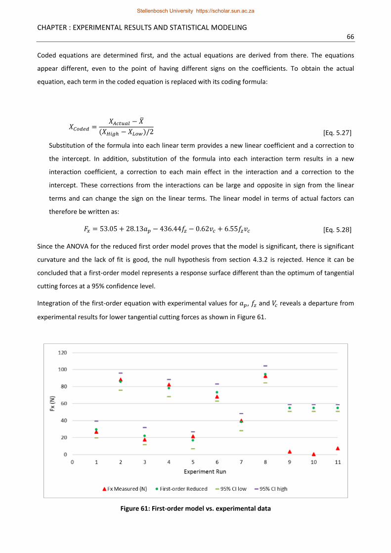
CHAPTER : EXPERIMENTAL RESULTS AND STATISTICAL MODELING 66
Coded equations are determined first, and the actual equations are derived from there. The equations
appear different, even to the point of having different signs on the coefficients. To obtain the actual
equation, each term in the coded equation is replaced with its coding formula:
𝑋𝐶𝑜𝑑𝑒𝑑 =𝑋𝐴𝑐𝑡𝑢𝑎𝑙 − �̅�
(𝑋𝐻𝑖𝑔ℎ − 𝑋𝐿𝑜𝑤)/2
[Eq. 5.27]
Substitution of the formula into each linear term provides a new linear coefficient and a correction to
the intercept. In addition, substitution of the formula into each interaction term results in a new
interaction coefficient, a correction to each main effect in the interaction and a correction to the
intercept. These corrections from the interactions can be large and opposite in sign from the linear
terms and can change the sign on the linear terms. The linear model in terms of actual factors can
therefore be written as:
𝐹𝑥 = 53.05 + 28.13𝑎𝑝 − 436.44𝑓𝑧 − 0.62𝑣𝑐 + 6.55𝑓𝑧𝑣𝑐 [Eq. 5.28]
Since the ANOVA for the reduced first order model proves that the model is significant, there is significant
curvature and the lack of fit is good, the null hypothesis from section 4.3.2 is rejected. Hence it can be
concluded that a first-order model represents a response surface different than the optimum of tangential
cutting forces at a 95% confidence level.
Integration of the first-order equation with experimental values for 𝑎𝑝, 𝑓𝑧 and 𝑉𝑐 reveals a departure from
experimental results for lower tangential cutting forces as shown in Figure 61.
Figure 61: First-order model vs. experimental data
Stellenbosch University https://scholar.sun.ac.za
CHAPTER : EXPERIMENTAL RESULTS AND STATISTICAL MODELING 67
The first order model from equation 5.28 is able to predict the tangential cutting forces well along the
higher tangential cutting force values, but prediction is unsatisfactorily along the lower cutting force data
points. Cutting forces for experiment run 9, 10 and 11 are not predicted accurately despite the model’s
non-significant lack of fit and large R-squared value. This variation at lower cutting forces is due to the
curvature that was found during the ANOVA. The first-order model does not represent the curvature
adequately. Therefore it is worth testing if a second-order or quadratic model may provide an improvement
upon the first-order model.
5.5.7 Fitting of a Quadratic Model
A quadratic model represents curvature more adequately due to the addition of second order terms to the
equation. A second order equation typically assumes the following form [75] [76]:
𝑦 = 𝛽0 + 𝛽1𝑥1 + 𝛽2𝑥2 + 𝛽12𝑥1𝑥2 + 𝛽11𝑥112 + 𝛽22𝑥2
2 + 𝜀
The construction of the initial ANOVA for the second order model follows the same method as the first
order model, with the exception of the squared term 𝐴2, which represents the curvature. Terms 𝐵2 and 𝐶2
are omitted here, because they are non-significant terms. The model sum of squares therefore now
includes the curvature sum of squares, which becomes 𝐴2 and lack of fit is re-calculated:
𝑆𝑆𝐴 =(225.03)2
8(1)= 6329.81
𝑆𝑆𝐵 =(27.51)2
8(1)= 94.60
𝑆𝑆𝐶 =(7.27)2
8(1)= 6.61
𝑆𝑆𝐴𝐵 =(9.17)2
8(1)= 10.51
𝑆𝑆𝐴𝐶 =(−26.91)2
8(1)= 90.52
𝑆𝑆𝐵𝐶 =(58.01)2
8(1)= 420.65
𝑆𝑆𝐶𝑢𝑟𝑣𝑒 => 𝑆𝑆𝐴2 = 5636.49
𝑆𝑆𝑀𝑜𝑑𝑒𝑙 = 𝑆𝑆𝐴 + 𝑆𝑆𝐵 + 𝑆𝑆𝐶 + 𝑆𝑆𝐴𝐵 + 𝑆𝑆𝐵𝐶 + 𝑆𝑆𝐴𝐶 + 𝑆𝑆𝐴2
= 6329.81 + 94.60 + 6.61 + 10.51 + 90.52 + 420.65 + 5636.49
= 12589.18
From equation 5.10, the total sum of squares is 12615.85 and therefore from equation 5.11:
Stellenbosch University https://scholar.sun.ac.za

CHAPTER : EXPERIMENTAL RESULTS AND STATISTICAL MODELING 68
𝑆𝑆𝑇𝑜𝑡𝑎𝑙 = 𝑆𝑆𝑀𝑜𝑑𝑒𝑙 + 𝑆𝑆𝐸𝑟𝑟𝑜𝑟 + 𝑆𝑆𝐿𝑜𝐹
12615.85 = 12589.18 + 25.83 + 𝑆𝑆𝐿𝑜𝐹
𝑆𝑆𝐿𝑜𝐹 = 0.84
And the residual sum of squares is the sum of 𝑆𝑆𝐿𝑜𝐹 and 𝑆𝑆𝐸𝑟𝑟𝑜𝑟:
𝑆𝑆𝑅𝑒𝑠 = 𝑆𝑆𝐿𝑜𝐹 + 𝑆𝑆𝐸𝑟𝑟𝑜𝑟
= 0.84 + 25.83
= 26.67
The MSE’s are:
𝑀𝑆𝐴 =6329.81
1= 6329.81
𝑀𝑆𝐵 =94.60
1= 94.60
𝑀𝑆𝐶 =6.61
1= 6.61
𝑀𝑆𝐴𝐵 =10.51
1= 10.51
𝑀𝑆𝐴𝐶 =90.52
1= 90.52
𝑀𝑆𝐵𝐶 =420.65
1= 420.65
𝑀𝑆𝐴2 =5636.49
1= 5636.49
𝑀𝑆𝐿𝑜𝐹 =0.84
1= 0.84
𝑀𝑆𝐸𝑟𝑟𝑜𝑟 =25.83
2= 12.91
𝑀𝑆𝑅𝑒𝑠 =26.67
3= 8.89
𝑀𝑆𝑀𝑜𝑑𝑒𝑙 =12589.18
7= 1798.45
The F-Values and p-values for the second-order ANOVA are now calculated. The hypothesis to determine
the significance of the model is:
The parameter of interest is the model terms.
Thus the test statistic,
Stellenbosch University https://scholar.sun.ac.za

CHAPTER : EXPERIMENTAL RESULTS AND STATISTICAL MODELING 69
𝐹0 =𝑀𝑆𝑀𝑜𝑑𝑒𝑙
𝑀𝑆𝐸𝑟𝑟𝑜𝑟
Tests the hypotheses,
𝐻0: 𝛽1 = 𝛽2 = 𝛽3 = 𝛽12 = 𝛽13 = 𝛽23 = 𝛽123 = 0
𝐻1: 𝑎𝑡 𝑙𝑒𝑎𝑠𝑡 𝑜𝑛𝑒 𝛽 ≠ 0
The selected confidence level is 95% (𝛼 = 0.05).
Reject 𝐻0 if 𝐹 > 𝐹𝑐𝑟𝑖𝑡𝑖𝑐𝑎𝑙 where 𝐹0.05,7,2 = 19.35
𝑀𝑆𝑀𝑜𝑑𝑒𝑙 = 1798.45, 𝑀𝑆𝐸𝑟𝑟𝑜𝑟 = 19.35
𝐹0 =𝑀𝑆𝑀𝑜𝑑𝑒𝑙
𝑀𝑆𝐸𝑟𝑟𝑜𝑟=
1798.45
19.35= 92.94
The p-value is 0.0106.
Since 𝐹 = 92.94 and 92.94 > 8.89, reject null hypothesis and conclude that the model is significant.
The p-value of 0.01059 indicates that there is only a 1.06% chance that a Model F-Value this large could
occur due to noise.
The hypothesis for the test of lack of fit is:
The parameter of interest is the lack of fit of the equation.
Thus the test statistic,
𝐹0 =𝑀𝑆𝐿𝑜𝑓
𝑀𝑆𝐸𝑟𝑟𝑜𝑟
Tests the hypotheses,
𝐻0: 𝑇ℎ𝑒𝑟𝑒 𝑖𝑠 𝑛𝑜 𝑙𝑎𝑐𝑘 𝑜𝑓 𝑓𝑖𝑡
𝐻1: 𝑇ℎ𝑒𝑟𝑒 𝑖𝑠 𝑎 𝑙𝑎𝑐𝑘 𝑜𝑓 𝑓𝑖𝑡
The selected confidence level is 95% (𝛼 = 0.05).
Reject 𝐻0 if 𝐹 > 𝐹𝑐𝑟𝑖𝑡𝑖𝑐𝑎𝑙 where 𝐹0.05,1,2 = 18.51
𝑀𝑆𝐿𝑜𝑓 = 0.84, 𝑀𝑆𝐸𝑟𝑟𝑜𝑟 = 12.91
𝐹0 =𝑀𝑆𝐿𝑜𝑓
𝑀𝑆𝐸𝑟𝑟𝑜𝑟=
0.84
12.91= 0.065
The p-value is 0.8227.
Since 𝐹 = 12.91 and 12.91 < 18.51, we cannot reject the null hypothesis and conclude: The "Lack of
Fit F-value" of 0.065 implies the Lack of Fit is not significant relative to the pure error. There is a 82.27%
chance that a "Lack of Fit F-value" this large could occur due to noise. Non-significant lack of fit is good.
We want the model to fit.
Table 15: ANOVA for second-order model
Source Sum of Squares
𝒅𝒇 Mean
Square F-Value
p-value Prob > F
Comment
Stellenbosch University https://scholar.sun.ac.za

CHAPTER : EXPERIMENTAL RESULTS AND STATISTICAL MODELING 70
Model 12589.18 7 1798.45 92.94 0.0106 significant
A-𝑎𝑝 6329.81 1 6329.81 712.08 0.0001
B-𝑓𝑧 94.60 1 94.60 10.64 0.0471
C-𝑣𝑐 6.61 1 6.61 0.74 0.4520
AB 10.51 1 10.51 1.18 0.3564
AC 90.52 1 90.52 10.18 0.0497
BC 420.65 1 420.65 47.32 0.0063
A2 5636.49 1 5636.49 634.08 0.0001
Residual 26.67 3 8.89
Lack of Fit 0.84 1 0.84 0.06 0.8227 not significant
Pure Error 25.83 2 12.91
Total 12615.85 10
The second-order model standard deviation of 2.98 is less than the first-order model standard deviation of
5.05 as shown in Table 16.
Table 16: Second-order model ANOVA supplementary table 1
Std. Dev. 2.98 R-Squared 0.9979
Mean 40.90 Adj R-Squared 0.9930
C.V. % 7.29 Pred R-Squared 0.9911
PRESS 111.78 Adeq Precision 34.7427
The CV of the second-order model (7.29%) is lower than the CV of the first-order model (12.35%). The
PRESS value of 111.78 for the second-order model is considerably less than the PRESS value of 782.51 for
the first-order model. The adjusted R-squared of 0.9930 is in better, reasonable agreement with the R-
squared of 0.9979 when compared to the first-order model. The signal to noise ratio of 34.74 shows
improvement over the first order model signal to noise ratio of 24.2619.
Table 17: Second-order model ANOVA supplementary table 2
Factor Coefficient Estimate
df Standard
Error 95% CI
Low 95% CI High
VIF
Intercept 3.94 1 1.72 -1.54 9.42
A-𝑎𝑝 28.13 1 1.05 24.77 31.48 1
B-𝑓𝑧 3.44 1 1.05 0.08 6.79 1
C-𝑣𝑐 0.91 1 1.05 -2.45 4.26 1
AB 1.15 1 1.05 -2.21 4.50 1
AC -3.36 1 1.05 -6.72 -0.01 1
BC 7.25 1 1.05 3.90 10.61 1
A2 50.83 1 2.02 44.40 57.25 1
Coefficients are assigned to the second-order model terms in Table 17. The final equation in terms of the
coded factors for the model is:
𝐹𝑥 = 3.94 + 28.13𝑎𝑝 + 3.44𝑓𝑧 − 0.91𝑣𝑐 + 1.15𝑎𝑝𝑓𝑧 − 3.36𝑎𝑝𝑉𝑐 + 7.25𝑓𝑧𝑉𝑐 + 50.83𝑎𝑝2 [Eq. 5.29]
Stellenbosch University https://scholar.sun.ac.za

CHAPTER : EXPERIMENTAL RESULTS AND STATISTICAL MODELING 71
Substituting the formula from equation 5.27 into each quadratic term will result in a new quadratic
coefficient and a correction to the intercept:
𝐹𝑥 = 102.45 − 114.93𝑎𝑝 − 470.83𝑓𝑧 − 0.39𝑉𝑐 + 22.93𝑎𝑝𝑓𝑧 − 0.15𝑎𝑝𝑉𝑐 + 6.55𝑓𝑧𝑉𝑐 + 50.83𝑎𝑝2 [Eq. 5.30]
Integration of the second-order equation with experimental values for 𝑎𝑝, 𝑓𝑧 and 𝑣𝑐 shows improved
prediction ability for high and low values of measured tangential cutting force as shown in Figure 62.
Figure 62: Second-order model vs. experimental data
Cutting forces for experiment run 9, 10 and 11 are predicted more accurately due to the inclusion of the
curvature in the second-order model. The second-order predicted force values also show better agreement
with experimental values, when compared to the predicted values of the first-order model. This confirms
the improvements discussed with Table 16. The second-order model provides satisfactory results at a 95%
confidence level. Diagnostic plots can be constructed for further evaluation.
5.5.8 Diagnostic Plots Diagnostic plots provide a valuable tool for visual assessment of the ANOVA findings. A modest deviation
from normality can be observed in the normal plot of residuals as shown in Figure 63, but not enough to be
of concern. The residuals vs. predicted plot also reveals nothing unusual, nor does the plot for externalized
student residuals. Predicted vs. actual plot shows good performance, including the centre points.
Stellenbosch University https://scholar.sun.ac.za

CHAPTER : EXPERIMENTAL RESULTS AND STATISTICAL MODELING 72
Figure 63: Residual and predictive plots
The Box-Cox plot for the power transforms that were performed on the primary data before the ANOVA
was performed, reveals no further requirements as shown in Figure 64. The ANOVA and diagnostic plots
provide satisfactory results of a significant second-order model that fits the design space.
Despite the suboptimal nature of the model, results still provide the opportunity to assess the model within
the selected response surface. The model is not fitted to the optimal response surface, therefore significant
predictions about any values outside of the experimental area cannot be made at the 95% confidence level.
Stellenbosch University https://scholar.sun.ac.za
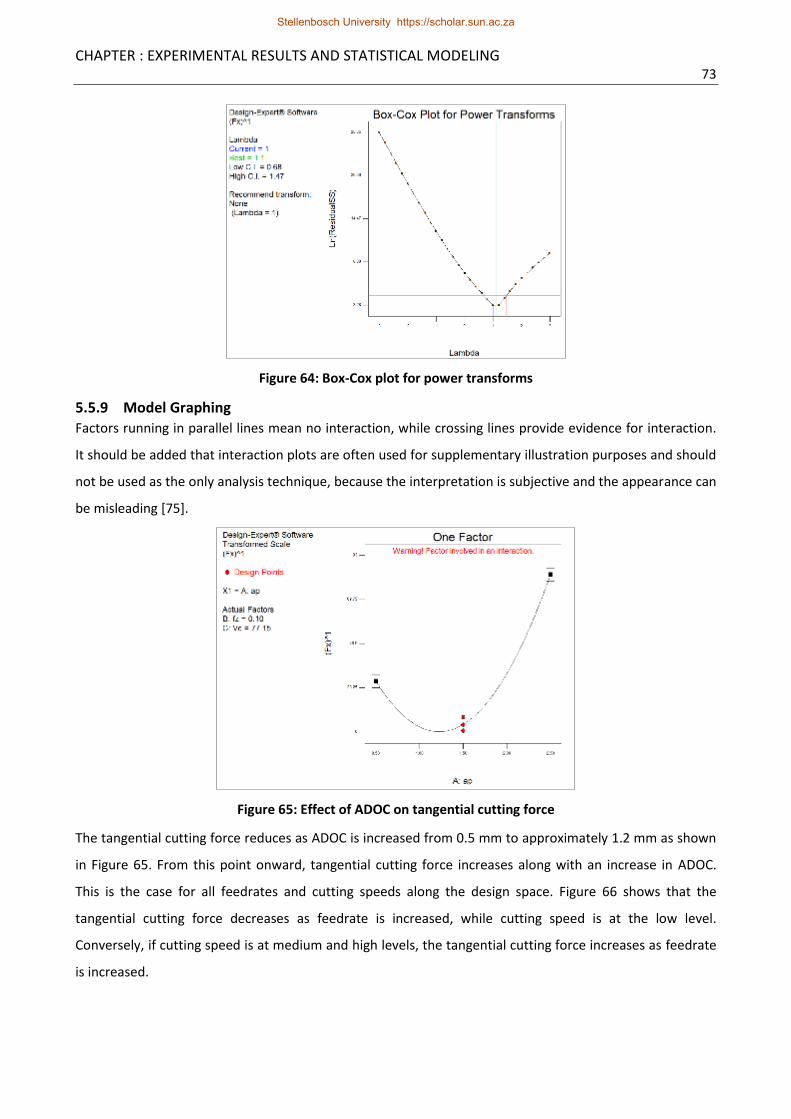
CHAPTER : EXPERIMENTAL RESULTS AND STATISTICAL MODELING 73
Figure 64: Box-Cox plot for power transforms
5.5.9 Model Graphing
Factors running in parallel lines mean no interaction, while crossing lines provide evidence for interaction.
It should be added that interaction plots are often used for supplementary illustration purposes and should
not be used as the only analysis technique, because the interpretation is subjective and the appearance can
be misleading [75].
Figure 65: Effect of ADOC on tangential cutting force
The tangential cutting force reduces as ADOC is increased from 0.5 mm to approximately 1.2 mm as shown
in Figure 65. From this point onward, tangential cutting force increases along with an increase in ADOC.
This is the case for all feedrates and cutting speeds along the design space. Figure 66 shows that the
tangential cutting force decreases as feedrate is increased, while cutting speed is at the low level.
Conversely, if cutting speed is at medium and high levels, the tangential cutting force increases as feedrate
is increased.
Stellenbosch University https://scholar.sun.ac.za

CHAPTER : EXPERIMENTAL RESULTS AND STATISTICAL MODELING 74
As cutting speed increases, the tangential cutting force decreases, as shown in Figure 67. This is only the
case at the low level of feedrate. The tangential cutting force increases as cutting speed increases at the
medium and high levels of feed per tooth.
Stellenbosch University https://scholar.sun.ac.za

CHAPTER : EXPERIMENTAL RESULTS AND STATISTICAL MODELING 75
Figure 66: Effect of feed per tooth on tangential cutting force at different cutting speeds
Stellenbosch University https://scholar.sun.ac.za

CHAPTER : EXPERIMENTAL RESULTS AND STATISTICAL MODELING 76
Figure 67: Effect of cutting speed on tangential cutting force at different feedrates
Stellenbosch University https://scholar.sun.ac.za
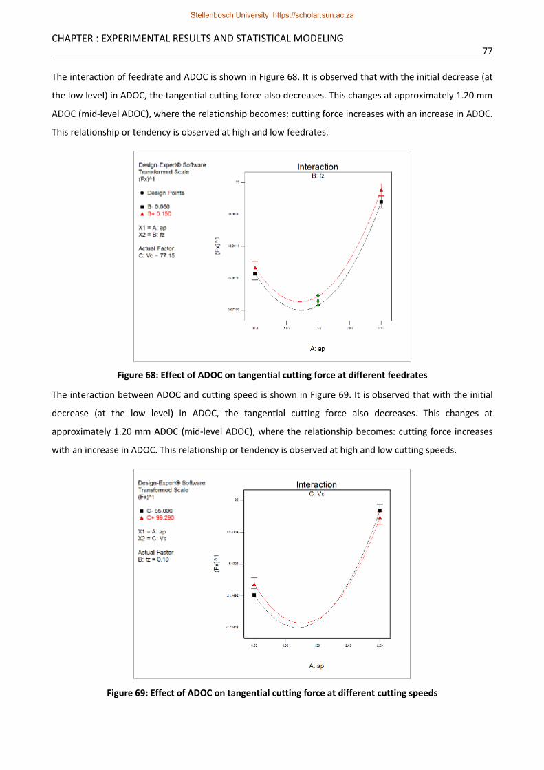
CHAPTER : EXPERIMENTAL RESULTS AND STATISTICAL MODELING 77
The interaction of feedrate and ADOC is shown in Figure 68. It is observed that with the initial decrease (at
the low level) in ADOC, the tangential cutting force also decreases. This changes at approximately 1.20 mm
ADOC (mid-level ADOC), where the relationship becomes: cutting force increases with an increase in ADOC.
This relationship or tendency is observed at high and low feedrates.
Figure 68: Effect of ADOC on tangential cutting force at different feedrates
The interaction between ADOC and cutting speed is shown in Figure 69. It is observed that with the initial
decrease (at the low level) in ADOC, the tangential cutting force also decreases. This changes at
approximately 1.20 mm ADOC (mid-level ADOC), where the relationship becomes: cutting force increases
with an increase in ADOC. This relationship or tendency is observed at high and low cutting speeds.
Figure 69: Effect of ADOC on tangential cutting force at different cutting speeds
Stellenbosch University https://scholar.sun.ac.za
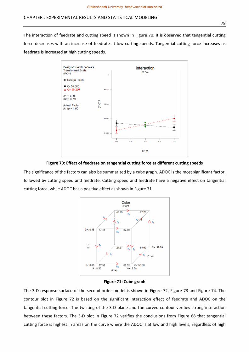
CHAPTER : EXPERIMENTAL RESULTS AND STATISTICAL MODELING 78
The interaction of feedrate and cutting speed is shown in Figure 70. It is observed that tangential cutting
force decreases with an increase of feedrate at low cutting speeds. Tangential cutting force increases as
feedrate is increased at high cutting speeds.
Figure 70: Effect of feedrate on tangential cutting force at different cutting speeds
The significance of the factors can also be summarized by a cube graph. ADOC is the most significant factor,
followed by cutting speed and feedrate. Cutting speed and feedrate have a negative effect on tangential
cutting force, while ADOC has a positive effect as shown in Figure 71.
Figure 71: Cube graph
The 3-D response surface of the second-order model is shown in Figure 72, Figure 73 and Figure 74. The
contour plot in Figure 72 is based on the significant interaction effect of feedrate and ADOC on the
tangential cutting force. The twisting of the 3-D plane and the curved contour verifies strong interaction
between these factors. The 3-D plot in Figure 72 verifies the conclusions from Figure 68 that tangential
cutting force is highest in areas on the curve where the ADOC is at low and high levels, regardless of high
Stellenbosch University https://scholar.sun.ac.za
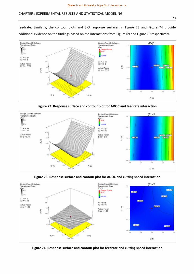
CHAPTER : EXPERIMENTAL RESULTS AND STATISTICAL MODELING 79
feedrate. Similarly, the contour plots and 3-D response surfaces in Figure 73 and Figure 74 provide
additional evidence on the findings based on the interactions from Figure 69 and Figure 70 respectively.
Figure 72: Response surface and contour plot for ADOC and feedrate interaction
Figure 73: Response surface and contour plot for ADOC and cutting speed interaction
Figure 74: Response surface and contour plot for feedrate and cutting speed interaction
Stellenbosch University https://scholar.sun.ac.za
CHAPTER : EXPERIMENTAL RESULTS AND STATISTICAL MODELING 80
5.6 CONCLUSIONS AND RECOMMENDATIONS
The experimental data collected for the tangential cutting force follows a left-skewed normal distribution
and had to be transformed with application of a power transformation for modeling and analysis purposes.
A first-order model provided a significant fit to the data at the 95% confidence level, but was unable to
predict tangential cutting forces at low levels. The alternative research hypothesis was statistically
significant, while the null hypothesis was rejected. The presence of significant curvature means that: “A
first-order model represents a response surface different than the optimum of tangential cutting forces”.
Hence a second-order model was fitted to the data. The second-order model significantly represents a
response surface with curvature that is close to the optimum response surface. The second-order equation
can be used to predict cutting forces within the design space at a 95% confidence level.
The model can be improved to represent the optimal response surface for this process through
augmentation towards a central composite design. Six axial or star points can be added to the existing
experimental data, which means that six additional experiments should be conducted. These six additional
experiments are to be performed under the exact conditions as the first set of experiments, i.e. the same
work material, milling machine setup, cutting tools and cutting strategy.
The examination of machinability factors such as surface finish, tool wear rate and chip control revealed no
abnormalities. The surface finish achieved during experimentation is comparable to the surface finish
requirements for finishing in some cases. Therefore the Kennametal KSRM63A04RC20BB cutter with
RCGX2006M0SGF inserts is recommended for roughing as successive finishing operations would be kept to
a minimum. Tool wear followed a uniform pattern for the majority of cutting experiments and is evident of
cutting under normal conditions. The analysis of cutting chips verified findings from literature and provided
evidence about the temperature and chip evacuation at the cutting interface.
Stellenbosch University https://scholar.sun.ac.za

CHAPTER : PRACTICAL WORK WITH INDUSTRY PARTNER 81
CHAPTER 6
PRACTICAL WORK WITH INDUSTRY PARTNER
6.1 INTRODUCTION The funding contract for this study requires technology transfer to an industrial partner. The goal of this
part of the project is therefore to transfer academic knowledge in a practical way to improve the
productivity of the industry partner’s current processes. Hence, the project is focused on a larger volume
product, where improvements, if any, would make the largest impact on overall productivity.
The chosen component for the project is a lug machined from stainless steel (Figure 75). Daliff Precision
Engineering manufactures an annual volume of approximately 100 lugs for Airbus. Daliff Engineering also
has contracts with companies such as Denel and Boeing, though annual volumes for these clients are lower.
The project had to coincide with a scheduled production window at the workshop.
The component for comparison (Figure 75) is machined from Aubert & Duval’s X15U5W 15-5 PH Stainless
Steel. The Stainless Steel was hardened for four hours at 550°C. Its Brinell hardness factor is 357 HBW and
tensile strength is 1126 N/mm2. These material characteristics are similar to Ti-6Al-4V (336 HBW, 950
N/mm2), with the exception of the difference in thermal conductivity. X15U5W 15-5 PH Stainless Steel has
a thermal conductivity of 16 W.m/m2. °C, compared to the thermal conductivity of Ti-6Al-4V (6.7
W.m/m2.°C) [39] [86]. The forces and power required for machining the two materials is expected to be
similar, with accelerated tool wear for Ti-6Al-4V.
Figure 75: Airbus lug component, 15-5 PH Stainless Steel (dimensions in mm)
The lug is currently fabricated on a Deckel Maho DMU 60, 5-axis milling machine. The Deckel Maho has an
initial investment cost of R4.5M. The current process times for machining the component on the Deckel
Maho are summarised in Figure 76. The roughing process occupies 73% of the current total machining time.
Stellenbosch University https://scholar.sun.ac.za

CHAPTER : PRACTICAL WORK WITH INDUSTRY PARTNER 82
Therefore this project is focused on improving the roughing process and subsequently reducing the
required machining time of the Airbus lug.
Figure 76: Current machining processes and times for Airbus lug
6.2 MACHINE TOOL, INSERTS AND WORKPIECE MOUNTING
In addition to the Deckel Maho, Daliff Precision Engineering has a Leadwell V-50L (3-axis) milling machine in
the workshop. The Leadwell milling machine’s cost is considerably less than the Deckel Maho at R1.6M, and
was therefore utilised for the purpose of comparative testing during this project. The Deckel Maho’s 5-axes
are not essential for the machining of the Airbus lug if recent developments are utilised in cutting tools and
hence process design. Migration of the roughing process to the Leadwell alone, already provides a 2.8
times saving due to the difference in machine cost per hour.
Figure 77: Kennametal Beyond Blast KSRM cutter ad RCGX round inserts
Roughing tools for the project are the Kennametal (Figure 77) and ISCAR (Figure 78) cutters with their
respective inserts. The ISCAR cutter has a positive-neutral geometry. Each cutter that was tested has four
Stellenbosch University https://scholar.sun.ac.za

CHAPTER : PRACTICAL WORK WITH INDUSTRY PARTNER 83
inserts. The Kennametal cutter has through spindle and split tool cooling. The Leadwell V-50L is able to
produce three bar pressure for nozzle and through spindle cooling.
Figure 78: ISCAR EWX cutter and H600 hexagonal inserts
The 15-5 PH stainless steel billets for the Airbus lugs were clamped to a pedestal that was clamped to the
machine bed (Figure 79). The pedestal and clamp is manufactured from mild steel. The billet is attached to
the pedestal by four screws in the bottom of the flange assembly. The flange is held together with two M12
screws (one in each opposing corner).The four holes in the bottom of the billet are pre-drilled. The pedestal
is then attached to the machine bed with two M10 screws (also one in each opposing corner).
Figure 79: Airbus "lug" clamping method on Leadwell V-50L
The cutting parameters such as feed per tooth (𝑓𝑧), ADOC (𝑎𝑝) and revolutions per minute (𝑛) required
process improvement for operation with the Leadwell machine to ensure more productive cutting
conditions.
Stellenbosch University https://scholar.sun.ac.za

CHAPTER : PRACTICAL WORK WITH INDUSTRY PARTNER 84
6.3 PRODUCTIVITY CALCULATIONS
Productivity formulae are often provided by the tool manufacturer in the technical section of the cutting
tool manuals for practical application in the workshop. In addition it was found that online productivity
calculators on the tool manufacturer websites employ the same formulae. These formulae are required to
calculate tool-specific productivity factors such as MRR, table feed, cutting speed, and cutting power for
example.
6.3.1 Tool Wear Factor The tool wear factor is a constant that corresponds to different tool wear rates with varying cutting forces.
The tool wear factor (𝐶𝑤) is needed for further cutting force related calculations. The tool wear factor for a
determined cutting operation can be referenced from Table 18, as prepared by Oberg [87]:
Table 18: Tool wear factors [87]
Milling type 𝒂𝒑 (mm) 𝒇𝒛 (mm) 𝑪𝒘
Light 0.5 to 2.5 0.08 to 0.15 1.1
Medium 2.5 to 5 0.15 to 0.25 1.2
Heavy Duty 5 to 10 0.25 to 1.0 1.3
6.3.2 Effective Cutting Diameter
The cutting speed is dependent on the effective cutting diameter (𝐷𝑚𝑎𝑥) at a specific axial depth (𝑎𝑝). With
the Kennametal inserts, the effective cutting diameter (𝐷𝑚𝑎𝑥) is dependent on the ADOC. The equation for
effective cutting diameter for the Kennametal cutter at a specific depth is [80]:
𝐷𝑚𝑎𝑥.𝑅 = 𝐷𝑐 + √𝐷𝑖2 − (𝐷𝑖 − 2𝑎𝑝)2
[Eq. 6.1]
Where 𝐷𝑚𝑎𝑥.𝑅 is the effective cutting diameter (mm), 𝐷𝑐 is the cutter body diameter (mm), 𝐷𝑖 is the insert
diameter (mm) and 𝑎𝑝 is the ADOC (mm). This equation is only applicable for use with round inserts, hence
the addition of “R” in the notation.
6.3.3 Radial Engagement Ratio and Machinability Factor
This ratio is the relationship of the radial depth of cut (RDOC) of the cutting tool and workpiece, based on
effective cutting diameter. For example: The machinability factor (𝐶𝑚) is assumed to be 1.20 for a W/D
ratio of 0.67 ≤ W/D ≤ 1.0 for Ti-6Al-4V milling as shown in Table 19.
Table 19: Kennametal machinability factor table [80]
Machinability Factor (𝑪𝒎) W/D ≤ 0.67 0.67 ≤ W/D ≤ 1.0 W/D = 1.0
Carbon & Alloy Steels 1.0 1.15 1.3
Stainless Steel 2.0 2.15 2.3
Grey Cast Iron 1.0 1.15 1.3
Titanium Alloys 1.0 1.20 1.4
Stellenbosch University https://scholar.sun.ac.za

CHAPTER : PRACTICAL WORK WITH INDUSTRY PARTNER 85
Aluminium Alloys 1.0 1.05 1.1
Figure 80 illustrates how the W/D engagement factor is calculated by using the ratio of the RDOC to the
maximum effective diameter of the cutter.
Figure 80: Top view of cutter bodies - Engagement factor of 0.625 (left) and 1.0 (right)
Radial engagement is formulated as follows:
𝑊
𝐷=
𝑎𝑒
𝐷max
[Eq. 6.2]
6.3.4 Engagement Angle and Number of Teeth in Cut
Number of teeth in cut (𝑍𝑐) is a calculated factor for how many inserts are in the cut and is used in
calculating the tangential cutting force (𝐹𝑥). The amount of inserts in the cut is dependent on the following
parameters: Effective cutting diameter (𝐷𝑚𝑎𝑥), Width of cut (𝑎𝑒), Engagement angle (𝛼), Angle between
cutter centre line and cutter radius to the peripheral point of exit or entry (𝛼1), and number of inserts in
the cutter body (𝑍𝑛). For all force and power related calculations, the effective cutter diameter (𝐷𝑚𝑎𝑥)
needs to be used. The effective cutting diameter should not be confused with the cutter body diameter
(𝐷𝑐). There are two different scenarios for calculating the number of inserts in the cut. The first formula
assumes that:
𝐷𝑚𝑎𝑥
2< 𝑎𝑒 < 𝐷𝑚𝑎𝑥 [Eq. 6.3]
The cutter is engaged with the workpiece by more than half of the effective cutting diameter as illustrated
in Figure 81.
Stellenbosch University https://scholar.sun.ac.za

CHAPTER : PRACTICAL WORK WITH INDUSTRY PARTNER 86
Figure 81: Engagement Angle and number of inserts in cut for Dmax/2 < ae < Dmax [82]
𝑍𝑐 for 𝐷𝑚𝑎𝑥/2 < 𝑎𝑒 < 𝐷𝑚𝑎𝑥 is formulated as:
𝑍𝑐 = 𝑧 [90° + 𝑠𝑖𝑛−1 (
2𝑎𝑒−𝐷𝑚𝑎𝑥
𝐷𝑚𝑎𝑥)]
360° [Eq. 6.4]
Where:
𝑍𝑐 =𝑧 × 𝛼°
360°
And:
𝛼 = 90° + 𝛼1
Thus:
𝑠𝑖𝑛𝛼1 =𝐴𝐵
𝑂𝐵= [
𝑎𝑒 − (𝐷𝑚𝑎𝑥
2)
(𝐷𝑚𝑎𝑥
2)
] =2 [𝑎𝑒 − (
𝐷𝑚𝑎𝑥
2)]
𝐷𝑚𝑎𝑥=
2𝑎𝑒 − 𝐷𝑚𝑎𝑥
𝐷𝑚𝑎𝑥
Hence:
𝛼1 = 𝑠𝑖𝑛−12𝑎𝑒 − 𝐷𝑚𝑎𝑥
𝐷𝑚𝑎𝑥
The second formula assumes that the cutter is engaged with the workpiece by less than half of the effective
cutting diameter as illustrated in Figure 82. The formula is given as:
𝑎𝑒 <𝐷𝑚𝑎𝑥
2 [Eq. 6.5]
Stellenbosch University https://scholar.sun.ac.za

CHAPTER : PRACTICAL WORK WITH INDUSTRY PARTNER 87
Figure 82: Engagement Angle and number of inserts in cut for ae < Dmax/2 [82]
𝑍𝑐 for 𝑎𝑒 < 𝐷𝑚𝑎𝑥/2 is formulated as:
𝑍𝑐 = 𝑧 [90° − 𝑠𝑖𝑛−1 (
𝐷𝑚𝑎𝑥−2𝑎𝑒
𝐷𝑚𝑎𝑥)]
360° [Eq. 6.6]
Where:
𝑍𝑐 =𝑧 × 𝛼°
360°
And:
𝛼 = 90° − 𝛼1
Thus:
𝑠𝑖𝑛𝛼1 =𝐴𝐵
𝑂𝐵= [
(𝐷𝑚𝑎𝑥
2) − 𝑎𝑒
(𝐷𝑚𝑎𝑥
2)
] =2 [(
𝐷𝑚𝑎𝑥
2) − 𝑎𝑒]
𝐷𝑚𝑎𝑥=
𝐷𝑚𝑎𝑥 − 2𝑎𝑒
𝐷𝑚𝑎𝑥
Hence:
𝛼1 = 𝑠𝑖𝑛−1𝐷𝑚𝑎𝑥 − 2𝑎𝑒
𝐷𝑚𝑎𝑥
6.3.5 Cutting Force Required at the Spindle
To calculate the required tangential cutting force, (𝑓𝑥) the formula used is:
𝐹𝑥 = 𝑆 × 𝐴 × 𝑍𝑐 × 𝐶𝑚 × 𝐶𝑤 [Eq. 6.7]
Where 𝑆 = Ultimate strength of Ti-6Al-4V (N/mm2), 𝐴 is average cross sectional area of the chip (mm2), 𝑍𝑐 is
number of inserts in cut (Not to be confused with 𝑧), 𝐶𝑚 is machinability factor is a constant 1.2 (factor),
𝐶𝑤 is tool wear factor is a constant for Ti-6Al-4V milling = 1.2 [80].
6.3.6 Cutting Speed The cutting speed equation is:
Stellenbosch University https://scholar.sun.ac.za

CHAPTER : PRACTICAL WORK WITH INDUSTRY PARTNER 88
𝑣𝑐 = 𝐷𝑐 × 𝜋 × 𝑛
1000 [Eq. 6.8]
Where, 𝑣𝑐 is the cutting speed in m/min, 𝐷𝑐 is the cutter body diameter, 𝜋 is the constant of which the first
six digits are 3.14159 and 𝑛 is the spindle speed (rpm). The cutting speed is also referred to as the chip
velocity and is the speed at which chips are removed at the cutting interface. The cutting interface is
subjected to increased friction in cases where the cutting speed is high.
6.3.7 Table Feed Table feed is the speed at which the tool is moving in the cutting direction. It is expressed as mm/min. The
table feedrate is formulated as:
𝑣𝑓 = 𝑓𝑧 × 𝑛 × 𝑧 [Eq. 6.9]
Where 𝑣𝑓 is the table feed in mm/min, 𝑓𝑧 is feed per tooth (mm), 𝑛 is spindle speed (rpm), 𝑧 is the number
of inserts in cutter body. Feed per tooth is the thickness of chip material that each tooth removes with one
pass as per Figure 83. The number of revolutions per minute is represented by n (rpm).
Figure 83: Top view of an example of a face milling cutter body with z = 8 and fz = 0.25
6.3.8 Average Cross Sectional Area of Chip The average cross sectional area of the chip is a dynamic value calculated by the product of the instantaneous
cutting depth and feed per tooth at any given moment during the cut.
Figure 84: Average cross sectional area of chip according to insert geometry
The average cross sectional area of the chip is calculated as [82]:
𝐴 = 𝑎𝑝 × 𝑓𝑧 [Eq. 6.10]
Stellenbosch University https://scholar.sun.ac.za
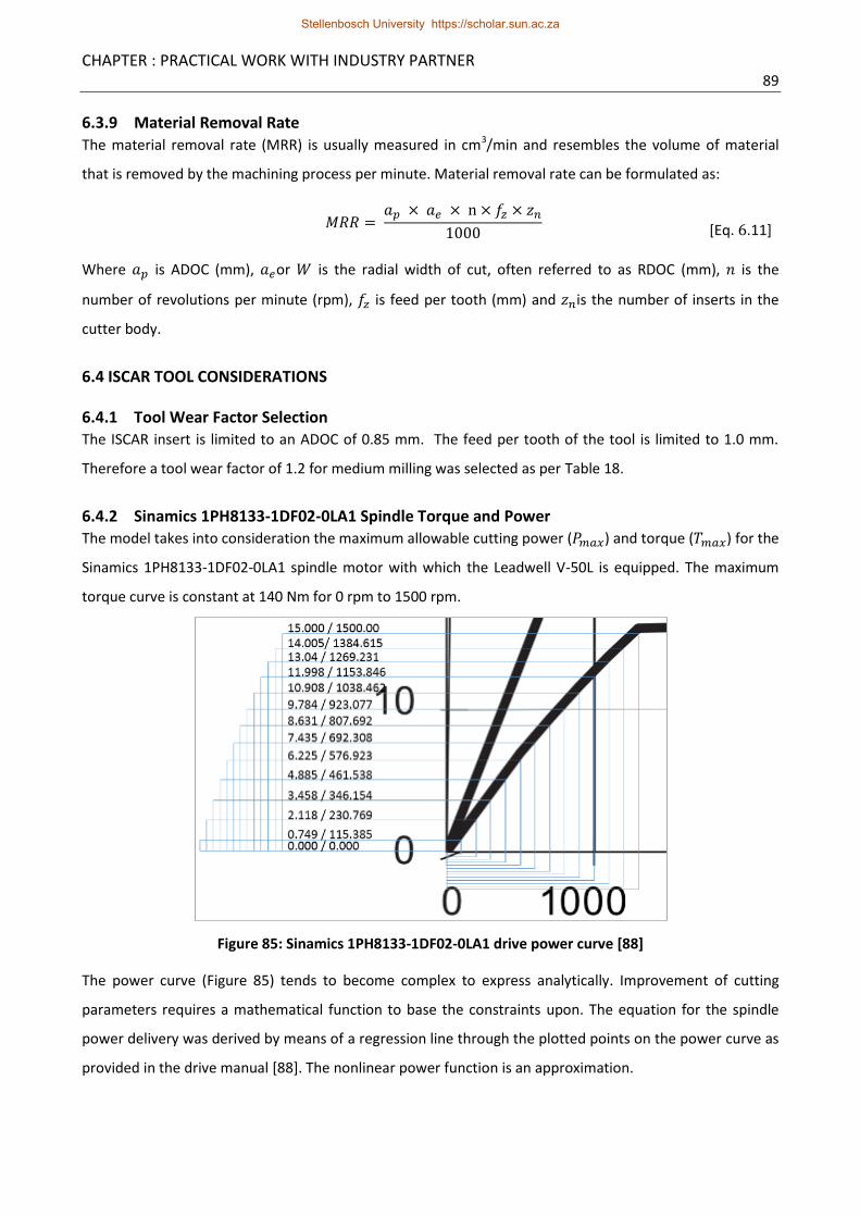
CHAPTER : PRACTICAL WORK WITH INDUSTRY PARTNER 89
6.3.9 Material Removal Rate
The material removal rate (MRR) is usually measured in cm3/min and resembles the volume of material
that is removed by the machining process per minute. Material removal rate can be formulated as:
𝑀𝑅𝑅 = 𝑎𝑝 × 𝑎𝑒 × n × 𝑓𝑧 × 𝑧𝑛
1000 [Eq. 6.11]
Where 𝑎𝑝 is ADOC (mm), 𝑎𝑒or 𝑊 is the radial width of cut, often referred to as RDOC (mm), 𝑛 is the
number of revolutions per minute (rpm), 𝑓𝑧 is feed per tooth (mm) and 𝑧𝑛is the number of inserts in the
cutter body.
6.4 ISCAR TOOL CONSIDERATIONS
6.4.1 Tool Wear Factor Selection The ISCAR insert is limited to an ADOC of 0.85 mm. The feed per tooth of the tool is limited to 1.0 mm.
Therefore a tool wear factor of 1.2 for medium milling was selected as per Table 18.
6.4.2 Sinamics 1PH8133-1DF02-0LA1 Spindle Torque and Power The model takes into consideration the maximum allowable cutting power (𝑃𝑚𝑎𝑥) and torque (𝑇𝑚𝑎𝑥) for the
Sinamics 1PH8133-1DF02-0LA1 spindle motor with which the Leadwell V-50L is equipped. The maximum
torque curve is constant at 140 Nm for 0 rpm to 1500 rpm.
Figure 85: Sinamics 1PH8133-1DF02-0LA1 drive power curve [88]
The power curve (Figure 85) tends to become complex to express analytically. Improvement of cutting
parameters requires a mathematical function to base the constraints upon. The equation for the spindle
power delivery was derived by means of a regression line through the plotted points on the power curve as
provided in the drive manual [88]. The nonlinear power function is an approximation.
Stellenbosch University https://scholar.sun.ac.za

CHAPTER : PRACTICAL WORK WITH INDUSTRY PARTNER 90
Figure 86: Sinamics SH 130 power vs. spindle speed function
The approximate equation for the maximum allowable spindle power is (from Figure 86):
𝑃𝑚𝑎𝑥 = −2𝐸−6𝑥2 + 0.0219𝑥 + 0.7565 [Eq. 6.12]
Where 𝑃𝑚𝑎𝑥 is the maximum allowable spindle power and 𝑥 is revolutions per minute at any given point.
6.4.3 Effective Cutting Diameter The effective cutting diameter for the KSRM cutter and RCGX inserts is determined through the application
of equation 6.1. On the other hand, the effective cutting diameter for the ISCAR cutter is calculated from
the geometric characteristics of its inserts and how they seat in the cutter body. The equation for effective
cutting diameter for the ISCAR insert at a specific depth can be derived as:
𝐷𝑚𝑎𝑥.𝐻 = 𝐷𝑐 + [2 (𝑎𝑝
tan 17)] + (3.46𝑎𝑝) [Eq. 6.13]
Where 𝐷𝑚𝑎𝑥.𝐻 is effective cutting diameter (mm), 𝑎𝑝 is the ADOC, 𝐷𝑐 is the diameter of cutter body (mm),
𝑡𝑎𝑛 17 is the tangent of the rake angle of the insert. Note the “H” added to the 𝐷𝑚𝑎𝑥 notation to specify
reference to the hexagonal ISCAR insert.
6.4.4 Other Cutting Parameters The machinability factor for 15-5 PH Stainless steel is 2.15 (from Table 19), taking into account an average
W/D ratio of 0.67 ≤ W/D ≤ 1.0 for the machining operation. The engagement angle and the number of teeth
in the cut is represented by equations 6.3 to 6.6 The cutting force required at the spindle is formulated by
using equation 6.7 and the cutting speed is calculated with equation 6.8. The table speed is determined
through equation 6.9 and the average cross sectional area of the undeformed chip is represented by
equation 6.10 with reference to Figure 84 and taking into account the insert geometry.
Material removal rate is calculated with equation 6.11 and the cutting power required at the spindle is
determined by substituting values for cutting speed and force into equation 6.14. The cutting torque
Stellenbosch University https://scholar.sun.ac.za

CHAPTER : PRACTICAL WORK WITH INDUSTRY PARTNER 91
required at the spindle is calculated using the required force and effective cutting diameter of a tool with
hexagonal inserts:
𝑇𝑠 = 𝐹𝑐 × 𝐷𝑚𝑎𝑥.𝐻
2000 [Eq. 6.14]
Where 𝑇𝑠 is the torque required at the spindle (Nm), 𝐹𝑐 is the cutting force and 𝐷𝑚𝑎𝑥 is the effective cutting
diameter of the round or hexagonal inserts (m), depending on which cutter is in use [45].
6.5 ISCAR EXPERIMENTS Scope for the adjustment of machining parameters according to the outputs from the nonlinear program
was provided by Daliff Engineering.
The computer-aided manufacturing (CAM) milling program followed a helical path down the outside of the
billet as shown in Figure 87. This was the case for both the ISCAR and Kennametal cutters.
Figure 87: Helical milling path for roughing of the billet
6.5.1 Nonlinear Programming The problem of maximising the material removal rate for the ISCAR cutter, depending on operational
constraints can be formulated as follows: Let: 𝑍𝑛 = 4; 𝑆 = 1126; 𝐷𝑐 = 22; 𝑎𝑒 = 28.5; 𝐶𝑤 = 1.2; 𝐶𝑚 = 2.15.
Equation 6.13 is used to calculate the 𝐷𝑚𝑎𝑥.𝐻 and equation 6.12 is used to calculate the power constraint
placed by the spindle. Equations 6.2 - 6.11 and 6.14 are used to calculate values for the cutting parameters.
Maximise:
𝑀𝑅𝑅 = 𝑎𝑝 × 𝑎𝑒 × 𝑛 × 𝑓𝑧 × 𝑧𝑛
1000 [Material Removal Rate]
Subject to:
𝑃𝑚𝑎𝑥 = −2𝐸−6𝑥2 + 0.0219𝑥 + 0.7565 [Spindle Power]
Stellenbosch University https://scholar.sun.ac.za

CHAPTER : PRACTICAL WORK WITH INDUSTRY PARTNER 92
𝑇𝑚𝑎𝑥 =𝐹𝑐 × 𝐷𝑚𝑎𝑥.𝐻
2000
[Spindle Torque]
𝑛 =1000 × 𝑣𝑐
𝜋 × 𝐷𝑐
[Spindle Speed]
For: 0 ≤ 𝑎𝑝 ≤ 0.85; 0 ≤ 𝑓𝑧 ≤ 1; 0 ≤ 𝑛 ≤ 1100; 0 ≤ 𝑇𝑚𝑎𝑥 ≤ 140; 0 ≤ 𝑃𝑚𝑎𝑥 ≤ 17.83 (𝑎𝑡 1100 𝑟𝑝𝑚)
6.5.2 Sensitivity Analysis of Nonlinear Programming Results
The following values were used in the nonlinear model: 𝑧𝑛 = 4; 𝑆 = 1126; 𝐷𝑐 = 22; 𝑎𝑒 = 28.5; 𝑊
𝐷=
0.934; 𝐶𝑚 = 2.15; 𝐶𝑤 = 1.2. Nonlinear program results are shown in Table 20:
Table 20: Nonlinear program results and sensitivity analysis
Parameter Type Value Status Slack Lagrange Multiplier
MRR Objective 81.28 cm3/min Obj. Function NA 0
𝑎𝑝 ≥ 0 Variable 0.85 mm Not Binding 0.85 0
𝑎𝑝 ≤ 0.85 Variable 0.85 mm Binding 0 38.35
𝑓𝑧 ≥ 0 Variable 0.76 mm Not Binding 0.76 0
𝑓𝑧 ≤ 1 Variable 0.76 mm Not Binding 0.24 0
𝑛 ≥ 0 Variable 1100 rpm Not Binding 1100 0
n ≤ 1100 Variable 1100 rpm Binding 0 0.05
𝑇𝑚𝑎𝑥 ≤ 140 Parameter 47.97 Nm Not Binding 92.03 0
𝑃𝑚𝑎𝑥 ≤ 17.83 Parameter 17.83 Kw Binding 0 4.56
Binding factors were the maximum allowable ADOC, spindle speed and available power at the spindle. Slack
values are 0.24 for the feed per tooth and 92.03 Nm for the available torque. The model returned a
maximum MRR of 81.28 cm3/min, while satisfying all constraints.
6.5.3 Experimental Results The cutting parameters for the ISCAR FF EWX D32-4-060-W32-05 cutter were programmed into the
Leadwell V-50L PLC. The parameters were taken from the nonlinear program outputs. They are: 𝑓𝑧 = 0.75
mm; 𝑎𝑝 = 0.85 mm; 𝑛 = 1100 rpm with a theoretically calculated MRR of 81.28 cm3/min.
Four billets were roughed out with the same inserts, not indexed between experiments. Parameters
remained unchanged between experiments. The total cutting time of the four billets was 18:54 minutes,
which results in an average of 4:43 minutes per billet. A surface roughness in excess of 320 μm, which is the
maximum measureable roughness for the Mitutoyo SJ-201P, was recorded. The experiments are tabulated
in Table 21:
Stellenbosch University https://scholar.sun.ac.za

CHAPTER : PRACTICAL WORK WITH INDUSTRY PARTNER 93
Table 21: ISCAR tabulated experimental results
# 𝒂𝒑 𝒇𝒛 𝒏 𝑻𝒎𝒂𝒙 𝑷𝒎𝒂𝒙 𝑫𝒎𝒂𝒙.𝑯 𝒁𝒄 𝒗𝒄 MRR 𝑻𝒔 𝑷𝒔 Time
(mm:ss) 𝑹𝒂
(μm)
1 0.85 0.75 1100 140 17.83 30.5 1.67 76.0 81.29 47.97 17.8 04:38 > 320
2 0.85 0.75 1100 140 17.83 30.5 1.67 76.0 81.29 47.97 17.8 04:40 > 320
3 0.85 0.75 1100 140 17.83 30.5 1.67 76.0 81.29 47.97 17.8 04:45 > 320
4 0.85 0.75 1100 140 17.83 30.5 1.67 76.0 81.29 47.97 17.8 04:55 > 320
The parameters for 𝑎𝑝, 𝑓𝑧 and 𝑛 are inputs. 𝑇𝑚𝑎𝑥 and 𝑃𝑚𝑎𝑥 are constraints for the nonlinear program. The
values underlined in the table are theoretically calculated. Cutting time was measured using a stopwatch to
indicate the time from cutter engagement with material to disengagement. Due to dry cutting during this
experiment, it is likely that chips were re-cut. The inserts were numbered and removed for microscope
analysis.
6.5.4 Microscope Analysis of ISCAR H600 WXCU 05T312T Inserts
Uniform flank wear was observed on the minor flanks of each of the four inserts (VB 1). Localized wear (VB
3) was observed on the major flank of all four inserts in the form of notches. Table 22 shows the measured
tool wear type detected on each flank face. Rake face wear was also inspected.
Cratering (KT 1) was found to have formed on all the insert rake faces. These phenomena could not be
quantified with respect to its dimensions, but the flank wear amounts could be measured using an Olympus
GX51 Microscope. The inserts were removed after the fourth experiment to examine tool wear over the
total cutting time of 18:54 minutes. The GX51 was set to 20x magnification (50 μm).
Table 22: ISCAR average uniform tool wear and maximum chip size (μm)
Insert # Minor Flank, Uniform
Wear (VB 1) Major Flank,
Localized Wear (VB 3)
1 30.82 171.52
2 37.59 178.88
3 41.13 176.96
4 43.26 100.80
Average 38.20 157.04
Testing time of approximately 20 minutes is classified as “short” in ISO 8988-1 : 1989 [55]. The standard
prescribes that under short testing, VB 1 of 200 μm is the maximum allowable wear for useful tool life.
Furthermore, VB 3 is limited to 1000 μm. Therefore the results obtained during the ISCAR tests fall well
within the guidelines set forth by the international standard for milling tool wear testing.
Stellenbosch University https://scholar.sun.ac.za

CHAPTER : PRACTICAL WORK WITH INDUSTRY PARTNER 94
Figure 88: ISCAR H600 WXCU 05T312T cratering on rake face (at 50 μm)
The cratering phenomena on the rake faces are indicated with red arrows in Figure 88. This is an indication
of high temperatures at the cutting interface due to the absence of coolant.
6.6 KENNAMETAL EXPERIMENTS
The KSRM63A04RC20BB cutter with four new RCGX2006M0SGF inserts was mounted on the Leadwell V-
50L. The workpiece was mounted using the existing pedestal clamping system as shown in Figure 89.
Figure 89: KSRM cutter and four new RCGX inserts on the Leadwell V-50L
Through spindle coolant was used for cutting experiments with the HPTSC-ST cutter. The maximum coolant
pressure provided by the Leadwell V-50L is 3 bar and is therefore not appropriate for use with the KSRM
cutter. Kennametal specifies a coolant pressure of at least 30 bar for all Beyond Blast applications [89].
6.6.1 Nonlinear Programming A maximum spindle speed of 900 rpm was selected for the first test to examine the cutter performance at
lower rpm’s due to the low coolant pressure. The problem of maximising the material removal rate for the
KSRM cutter, depending on operational constraints can now be formulated. Let: Zn = 4; S = 1126; Dc = 43; ae
Stellenbosch University https://scholar.sun.ac.za

CHAPTER : PRACTICAL WORK WITH INDUSTRY PARTNER 95
= 28.5; Cw = 1.2; Cm = 2.15. Eq. 6.25 is used to calculate the power constraint placed by the spindle. Eq. 6.1
is now used to calculate Dmax.R. Equations 6.1 - 6.12 and 6.14 are used to calculate values for the cutting
parameters.
Maximise:
𝑀𝑅𝑅 = 𝑎𝑝 × 𝑎𝑒 × 𝑛 × 𝑓𝑧 × 𝑧𝑛
1000 [Material Removal Rate]
Subject to:
𝑃𝑚𝑎𝑥 = −2𝐸−6𝑥2 + 0.0219𝑥 + 0.7565 [Spindle Power]
𝑇𝑚𝑎𝑥 =𝐹𝑐 × 𝐷𝑚𝑎𝑥.𝑅
2000
[Spindle Torque]
𝑛 =1000 × 𝑣𝑐
𝜋 × 𝐷𝑐
[Spindle Speed]
For: 0 ≤ 𝑎𝑝 ≤ 4.0; 0 ≤ 𝑓𝑧 ≤ 0.2; 0 ≤ 𝑛 ≤ 900; 0 ≤ 𝑇𝑚𝑎𝑥 ≤ 140; 0 ≤ 𝑃𝑚𝑎𝑥 ≤ 15.63 (𝑎𝑡 900 𝑟𝑝𝑚)
6.6.2 Sensitivity Analysis of Nonlinear Programming Results
The following values were used in the nonlinear model: 𝑧𝑛 = 4; 𝑆 = 1126; 𝐷𝑐 = 43; 𝑎𝑒 = 28.5; 𝑊
𝐷=
0.4831; 𝐶𝑚 = 2.15; 𝐶𝑤 = 1.2. The nonlinear program results are shown in Table 23:
Table 23: Nonlinear program results and sensitivity analysis
Parameter Type Value Status Slack Lagrange Multiplier
MRR Objective 62.24 cm3/min Obj. Function NA 0
𝑎𝑝 ≥ 0 Variable 4.0 mm Not Binding 4.0 0
𝑎𝑝 ≤ 4.0 Variable 4.0 mm Binding 0 1.0
𝑓𝑧 ≥ 0 Variable 0.15 mm Not Binding 0.15 0
𝑓𝑧 ≤ 0.2 Variable 0.15 mm Not Binding 0.05 0
𝑛 ≥ 0 Variable 900 rpm Not Binding 900 0
n ≤ 900 Variable 900 rpm Binding 0 0.05
𝑇𝑚𝑎𝑥 ≤ 140 Parameter 50.87 Nm Not Binding 89.13 3.98
𝑃𝑚𝑎𝑥 ≤ 15.63 Parameter 15.63 Kw Binding 0 0
Binding factors were the maximum allowable ADOC, spindle speed and available power at the spindle. Slack
values are 0.05 mm for the feed per tooth, and 89.13 Nm for the available torque. The model returned a
maximum MRR of 62.24 cm3/min, while satisfying all constraints.
Stellenbosch University https://scholar.sun.ac.za

CHAPTER : PRACTICAL WORK WITH INDUSTRY PARTNER 96
The cutting parameters were adjusted for each one of the five experiments with the KSRM cutter. The total
cutting time during the first experiment was 7:37 minutes. The inserts were indexed after every
experiment.
The cutting parameters were adjusted for experiment two as shown in Table 24. According to theoretically
calculated values, 𝑇𝑠 does not exceed 𝑇𝑚𝑎𝑥. The spindle power was theoretically calculated to be upon the
threshold of the approximated maximum allowable spindle power. During experiment two, the cutter
ceased in the cut, shattering the four inserts. As a results, tool wear could not be measured for experiment
one and two. Although undesirable for production purposes, the shattering inserts verify the calculated
theoretical power limit.
Table 24: Kennametal tabulated experiment results
# 𝒂𝒑 𝒇𝒛 𝒏 𝑻𝒎𝒂𝒙 𝑷𝒎𝒂𝒙 𝑫𝒎𝒂𝒙.𝑯 𝒁𝒄 𝒗𝒄 MRR 𝑻𝒔 𝑷𝒔 Time
(mm:ss) 𝑹𝒂
(μm)
1 4.00 0.15 900 140 15.63 59.0 0.98 121.6 62.24 50.87 15.63 07:37 0.57
2 5.66 0.32 683 140 12.80 61.0 0.99 131.0 141.69 170.70 12.21 NaN NaN
3 2.50 0.15 1953 140 22.72 56.2 1.02 345.0 87.22 7.54 1.54 05:24 0.57
4 2.50 0.17 2110 140 22.83 56.2 1.02 372.7 101.56 8.76 1.94 04:40 0.57
5 2.50 0.20 1500 140 21.03 56.2 1.02 265.0 87.00 12.72 2.00 05:10 0.57
The machine was reset, new inserts were attached and experiment three was initiated with different
machining parameters as shown in Table 24. The underlined values in the table are theoretically calculated.
During experiment three there was significant chatter, which caused chipping of the rake face on the RCGX
inserts. It was suspected that the pedestal clamp caused deflection and therefore the pedestal was
removed after experiment three and the workpiece was mounted directly to the machine bed.
During experiment four and five chatter was decreased, but tool chipping was still encountered. An average
surface roughness of 0.57 μm was measured on the inside diameter of billets one and three to five, using
the on-site laboratory’s Mitutoyo SJ-201P roughness tester. The total machining time for the four
successfully cut billets was 22:51 minutes with an average of 05:42 minutes per billet.
As a result of the low coolant pressure provided to the KSRM cutter, it is likely that chips were re-cut,
because adequate evacuation was not possible. In addition, effective chip lifting effect (Figure 14) could not
be achieved as the recommended minimum coolant pressure for this specific tool is 35 bar.
6.6.3 Microscope Analysis of Kennametal RCGX2006M0SGF Inserts
Inserts one to four were removed and analysed using an Olympus GX51 Microscope set to 5x magnification
(200 μm). Tool wear was measured for every experiment from the third experiment onwards. Due to the
inserts shattering during experiment two, it was impossible to recover these inserts for microscope
Stellenbosch University https://scholar.sun.ac.za

CHAPTER : PRACTICAL WORK WITH INDUSTRY PARTNER 97
analysis. However, inserts from experiments three, four and five provide tool wear evidence. Uniform flank
wear (VB 1) was observed on the minor flank and localised notching (VB 3) was observed on the major flank
as shown in Table 25.
Table 25: RCGX2006M0SGF insert wear
EXPERIMENT 3 EXPERIMENT 4 EXPERIMENT 5
Insert Minor Flank,
Uniform Wear (VB 1)
Major Flank, Localized
Wear (VB 3)
Minor Flank, Uniform
Wear (VB 1)
Major Flank, Localized
Wear (VB 3)
Minor Flank, Uniform
Wear (VB 1)
Major Flank, Localized
Wear (VB 3)
1 102.84 560.64 65.00 1040.64 33.85 211.20
2 72.41 691.20 61.04 839.68 34.61 515.84
3 74.34 1214.72 55.04 678.40 35.84 194.56
4 93.82 1018.88 63.98 529.92 38.11 157.44
Ave. 85.85 974.93 61.27 772.16 35.60 269.76
There is a reduction in the average uniform tool wear on the minor flank (VB 1) from experiment three to
experiment four due to the removal of the pedestal clamp. VB 1 was further reduced from experiment four
through five by application of more conservative cutting parameters. Similarly, the average size of the
localized notching observed on the major flanks was reduced from experiment three to five as shown in
Table 25. According to ISO 8988-1 : 1989 [55], the total uniform wear criteria falls under “short” testing,
because the average machining time per experiment was approximately five minutes. Therefore, the
specified criteria for the uniform tool wear on the minor flank (VB 1) is 200 μm and the localized wear (VB
3) limit is 1000 μm. In terms of these criteria, the RCGX2006M0SGF inserts conform to the ISO standard.
However, analysis of the rake faces revealed localized, macro chipping (CH 3) [55] as shown in (Figure 90 b).
The average chip length observed on the rake face is reduced from experiment three to five, due to
aforementioned factors as shown in Table 26.
Table 26: RCGX2006M0SGF insert chipping size (μm)
Insert # Exp. 3 Exp. 4 Exp. 5
1 1246.72 1268.48 none
2 1331.20 771.84 736.00
3 812.80 642.52 none
4 1112.32 505.60 none
Average 1125.76 797.11 736.00
ISO 8988-1 : 1989 [55] specifies the maximum chip length for macro chipping during a small testing time at
300 to 1000 μm. In terms of this criteria and also taking into consideration the observed degree of chipping
on the rake faces of the inserts, conditions for the RCGX2006M0SGF are not ideal.
Stellenbosch University https://scholar.sun.ac.za

CHAPTER : PRACTICAL WORK WITH INDUSTRY PARTNER 98
Figure 90: Kennametal tool wear: (a) Grooving, insert 4, exp. 4 (b) Flaking, insert 2, exp. 4 (at 200 μm)
The absence of rigid clamping and sufficient coolant pressure are the major contributing factors. The
removal of the pedestal clamping device did not eliminate the tool chipping, but the average chipping size
on the tool rake face was reduced.
6.7 PRODUCTIVITY AND SAVINGS The KSRM cutter is not a feasible solution for roughing on the Leadwell V-50L mainly because of the lack of
proper coolant pressure. Savings are interpreted in terms of the improvement of cutting parameters for the
ISCAR cutter. Figure 91 illustrates the effect of the reduced roughing time on total lug machining time. The
roughing time was reduced to an average of five minutes. This is a saving of 108 minutes per lug. It is an
annual time saving of 172.8 hours, based on an annual volume of 96 units. A total time saving of 95.57% is
achieved.
Figure 91: Airbus lug improved roughing time as percentage of total machining time
Taking into consideration the entire machining process of the Airbus lug (Figure 91) it is evident that the
roughing process now occupies 11% of the total time required to machine the component. This paves the
way for further improvement of other milling processes that occupy large quantities of time, such as the
Stellenbosch University https://scholar.sun.ac.za

CHAPTER : PRACTICAL WORK WITH INDUSTRY PARTNER 99
second surface finishing process (23%). Further improvements can be achieved in the exact same method
as was done with the ISCAR tool, keeping in mind that the tool geometry should be adapted to suit the new
milling tool in question. This is necessary so that an accurate 𝐷𝑚𝑎𝑥 value can be calculated, which
subsequently dictates the accuracy of force, power and torque estimations at any given machining
parameters.
6.8 ECONOMIC FEASIBILITY
The economic feasibility of split tools can be determined by comparing the ISCAR cutter’s cost model to
that of the split tools. The basis for comparison used is the cost per cm3 (In Rand currency) removed for
each tool. This can be expressed by the following formula as also used by Boeing Phantom Works during
tool life and feasibility experiments [90]:
𝑅/𝑐𝑚3 = [
𝑇𝑐
𝑇𝐿+
𝑅𝑚
60+ (
𝑅𝐿
60×
𝑇
𝑇𝐿)]
𝑀𝑅𝑅 [Eq. 6.15]
Where 𝑇𝑐 is the tool cost of the inserts, 𝑇𝐿 is the tool life in minutes (total), calculated by multiplying the
amount of insert edges or indexing positions with the tool life per edge, 𝑅𝑚 is the milling machine’s hourly
rate, 𝑅𝐿 is the labour rate per hour and 𝑇 is the tool change time in minutes. The data collected for milling
the Airbus lug is used to populate Table 27 and Table 28. The cost/cm3 is calculated by substituting values
into equation 6.15.
Table 27: ISCAR cutter cost calculations
T = 15 Tool change time (min)
Tc = R 928.40 Tool cost
TL = 114 Tool life (min)
Rm = R 450.00 Machine hourly rate (R/hr)
RL = R 50.00 Labour hourly rate (R/hr)
MRR = 81.28 cm3/min
Cost/cm3 = R 0.19 (from eq. 6.15)
Table 28: Kennametal split tool cost calculations
T = 15 Tool change time (min)
Tc = R 348.48 Tool cost
TL = 30 Tool life (min)
Rm = R 450.00 Machine hourly rate (R/hr)
RL = R 50.00 Labour hourly rate (R/hr)
MRR = 62.24 cm3/min
Cost/cm3 = R 0.31 (from eq. 6.15)
Stellenbosch University https://scholar.sun.ac.za

CHAPTER : PRACTICAL WORK WITH INDUSTRY PARTNER 100
The hourly machine rate and labour costs were obtained from the industry partner and the MRR’s used for
calculation were taken from the experimental results. Tool change time was measured during machining of
the Airbus lugs and recorded as an average of 15 minutes per cutter. This is the time required to index all
four inserts on each cutter. The ISCAR cutter provides a 63.16% reduction in cost per cm3. This difference in
cost can be attributed to the better tool life of the ISCAR inserts, compared to the split tool inserts, despite
the lower cost of the split tool inserts (62.47% lower).
Stellenbosch University https://scholar.sun.ac.za

CHAPTER 7: CONCLUSIONS AND RECOMMENDATIONS 101
CHAPTER 7
CONCLUSIONS AND RECOMMENDATIONS
7.1 CONCLUSIONS The examination of machinability factors such as surface finish, tool wear rate and chip control revealed no
abnormalities. Uniform tool wear was observed during experimentation with negligible occurrences of non-
uniform wear. Shearing of chips was observed at high cutting speeds, but according to findings from
literature, this is a beneficial phenomenon when machining Ti-6Al-4V as surface finish is improved during
shearing. Precision Coolant Technology assisted with chip lifting and evacuation. Further analysis of the cut
chips provided evidence about the low temperatures and thorough chip removal at the cutting interface.
The cutting experiments generated useful data for modeling of tangential cutting forces with split tools.
The primary research hypothesis was answered and the null hypothesis rejected. The research question
regarding the predictive tangential cutting force model is answered satisfactorily and a second-order model
fits the data at 95% confidence level. The predicted values show good agreement with experimental data
and the model can therefore be used to navigate the experimental design space. The existing experiment
design can be augmented by the addition of six star points to form a central composite design. This design
is preferred, when significant curvature is present as shown by the first-order model. A model fitted to the
data delivered by the central composite design will have to be tested for optimality, but evidence from
significant curvature suggests that the existing full factorial design was already rather close to the optimal
response surface. A model fitted to the optimal response surface would be valuable for predicting
tangential cutting forces for the entire process without being limited to the design space.
The ANOVA for the second-order model gives a clear indication of the significant factors that affected
cutting forces during experimentation. The interaction plots and 3-D response surfaces also show how
these factors affect each other by indicating interactions. The factors affecting cutting force are (1) ADOC,
(2) feedrate, and (3) cutting speed, respectively and in that order of significance. Regression analysis
revealed no relationship between cutting force vs. tool wear or cutting force vs. surface roughness.
The surface finish achieved during laboratory experimentation is highly satisfactory. The maximum surface
roughness on the outside diameter of the cut was reported as 1.26 micron that is below the requirement
for the final surface finish for the selected industry partner component. The high material removal rate
achieved during high levels of ADOC, feedrate and cutting speed promotes the feasibility of this cutter as a
roughing tool as successive finishing operations would be reduced. It should be added that the large inserts
and cutter diameter will limit the use of the tool to roughing out of large surface areas with large radius
corners.
Stellenbosch University https://scholar.sun.ac.za

CHAPTER 7: CONCLUSIONS AND RECOMMENDATIONS 102
7.2 RECOMMENDATIONS FOR INDUSTRY PARTNER
The ISCAR FF EWX cutter provided a higher MRR than the Kennametal KSRM on the Leadwell V-50L. The
improved MRR can be attributed to the ISCAR FF EWX cutter’s smaller effective tool diameter compared to
the Kennametal KSRM cutter (32mm vs. 63mm). Effective diameter directly affects the number of teeth in
the cut (𝑍𝑐) for a given radial engagement (𝑎𝑒). Since number of teeth in cut is a factor in calculating MRR,
it proves that higher radial immersion ratios (W/D) are more productive than smaller radial immersions
when only MRR is considered. Hence, in this case, due to the geometry of the component, the smaller
diameter cutter proved more efficient.
The measured tool wear of the ISCAR FF EWX (VB 1 and VB 3) after experiments 1-4 fall within the ISO
8988-1 : 1989 criteria for face milling tool testing [55]. Notching was observed on the major flank and
cratering was found on the rake face. It is recommended that coolant be used to improve tool life, more
specifically to reduce the cratering in the rake face of the ISCAR H600 WXCU 05T312T inserts.
The measured tool wear of the Kennametal RCGX inserts after experiments 3-5 is not in agreement with
the ISO 8988-1 : 1989 criteria. More specifically, the average chip size. The initial workpiece clamping
method contributed to the chipping of the Kennametal RCGX inserts during experiments one, two and
three.
Furthermore, the coolant pressure of 3 bar that is provided on the Leadwell V-50L is not sufficient for
roughing at high feedrates with the Kennametal KSRM cutter. These cutters are designed for use with
pressures of 30 bar and upward. Evidence suggests that adequate chip lifting was not achieved and
therefore chips were re-cut, accelerating the tool wear rate through elevated temperatures at the cutting
interface.
Notching was observed during experimentation with both cutters. According to the literature review,
notching occurs in cases where previously machined sections are re-machined [56]. This is the case with a
helical milling path as shown in Figure 87.
ISCAR tools cost 62.47% less per cm3 of material removed. For the purpose of this particular machining
process, taking into consideration operational and economic feasibility factors, it is recommended that the
ISCAR FF EWX D32-4-060-W32-05 cutter and H600 WXCU 05T312T inserts be utilized for future use. The
average major localized flank wear on the H600 WXCU 05T312T inserts was 157 μm for 18 minutes of
machining. This falls well within the tool life requirements set by the industry partner and ISO standards.
A 95.57% time saving was achieved by increasing the cutting parameters of an existing roughing process.
Other milling processes at Daliff Precision Engineering may be improved by means of the nonlinear
programming model that was created for this project. The model for this project was created using MS
Excel in a way that allows easy modification to accommodate different spindle power curves and cutter
Stellenbosch University https://scholar.sun.ac.za

CHAPTER 7: CONCLUSIONS AND RECOMMENDATIONS 103
geometries. The report explains in detail what is required to apply these changes for other processes. The
time required for adjusting the model is negligible compared to the savings that are made as a result.
In terms of the research problem, it is recommended that it becomes common practice for Daliff Precision
Engineering to analytically consider machining processes, if world class aerospace component machining is
desired. The feasibility of split tool milling at the industry partner was explored and it can be concluded
that it is not a feasible alternative at the moment, due to coolant pressure limitations on the Leadwell V-
50L. The operating characteristics of the KSRM cutter were explored in laboratory experiments and in
practice. The geometry of the selected aerospace component provides a challenge for the KSRM cutter.
Despite these findings, laboratory experiments provide evidence that suggests that the Kennametal KSRM
cutter holds the potential to save roughing time and reduce subsequent finishing processes. The KSRM
cutter provides a surface finish that matches the industry partner’s final finish requirement.
Stellenbosch University https://scholar.sun.ac.za

LIST OF REFERENCES 104
LIST OF REFERENCES
[1] H. Sibum, “Titanium and Titanium Alloys - From Raw Material to Semi-finished Products,” Advanced
Engineering Materials, vol. 5, no. 6, pp. 393-398, 4 July 2003.
[2] C. Cui, B. Hu, S. Liu and L. Zhao, “Titanium Alloy Production Technology, Market Prospects and Industry
Development,” Materials & Design, vol. 32, no. 3, pp. 1684-1691, March 2011.
[3] D. J. de Beer, “Establishment of Rapid Prototyping/Additive Manufacturing in South Africa,” The
Journal of The Southern African Institute of Mining and Metalurgy, vol. 111, no. 1, pp. 211-215, March
2011.
[4] G. Herlihy, “Metals Week,” Platts, vol. 83, no. 16, p. 22, 16 April 2012.
[5] R. Singh, Introduction to Basic Manufacture Process and Workshop Technology, Darya Ganj, New
Delhi: New Age International Publishers, 2006, p. 117.
[6] G. Lutering and J. C. Williams, Titanium (Engineering Materials and Processes), Berlin: Springer-Verlag
Berling Heidelberg, 2007, p. 60.
[7] J. C. Aurich and D. Dornfield, “Burrs - Analysis, Control and Removal,” in Proceedings to the CIRP
International Conference on Burrs, University of Kaiserslautern, 2009.
[8] D. Koen, Investigation of Novel Cooling Methods to Enhance Aerospace Component Manufacturing
Practices, Stellenbosch, Western Cape: Stellenbosch University, 2011, pp. 13, 47-52.
[9] G. A. Oosthuizen, Innovative Cutting Materials for Finish Shoulder Milling Ti-6Al-4V, Stellenbosch,
Western Cape: Stellenbosch University, 2009, pp. 38, 58-60, 101.
[10] B. North, “Why Metalcutting (Especially in Aerospace) is Such and Exciting Field,” in 5th Annual
Americas HTEC CNC Educators Conference, Phoenix, 2011.
[11] J. Cagan and C. M. Vogel, Creating Breakthrough Products: Revealing the Secrets that Drive Global
Innovation, New Jersey: Pearson Education, FT Press, 2012.
[12] H. Jeong, D. Y. Lee, M. G. Lee, S. W. Lee, K. H. Park and G. D. Yang, “Eco-Friendly Face Milling of
Titanium Alloy,” International Journal of Precision Engineering and Manufacturing, vol. 15, no. 6, pp.
1159-1164, June 2014.
[13] E. Chiapinni, M. Monno, Q. Semeraro, M. Strano and S. Tirelli, “Experimental Comparison Between
Traditional and Cryogenic Cooling Conditions in Rough Turning of Ti-6Al-4V,” Key Engineering
Materials, vol. 611, pp. 1174-1185, 2014.
[14] VOLUMILL, “US Air Force Announces Sustainable Manufacturing Successes,” Wright-Patterson Air
Force Base, Fairborn, 2011.
[15] Y. Ding and S. Y. Hong, “Cooling Approaches and Cutting Temperatures in Cryogenic Machining of Ti-
6Al-4V,” International Journal of Machine Tools and Manufacture, vol. 41, no. 10, pp. 1417-1437, 2001.
Stellenbosch University https://scholar.sun.ac.za

LIST OF REFERENCES 105
[16] F. Klocke, D. Lung, T. Cayli, B. Dobbeler and H. Sangermann, “Evaluation of Energy Efficiency in Cutting
Aerospace Materials with High-Pressure Cooling Lubricant Supply,” International Journal of Precision
Engineering and Manufacturing, vol. 15, no. 6, pp. 1179-1185, June 2014.
[17] J. Bernardin and I. Mudawar, “Experimental And Statistical Investigation Of Changes In Surface
Roughness Associated With Spray Quenching,” International Journal of Heat and Mass Transfer, vol.
39, no. 10, pp. 2023-2037, 1996.
[18] J. Bonney, R. B. da Silva, E. O. Ezugwu, Á. R. Machado and F. Wisley, “Tool Life and Wear Mechanisms
in High Speed Machining of Ti-6Al-4V Alloy with PCD Tools Under Various Coolant Pressures,” Journal
of Materials Processing Technology, vol. 213, no. 8, pp. 1459-1464, August 2013.
[19] E. O. Ezugwu, “Key Improvements in the Machining of Difficult-to-cut Aerospace Superalloys,” Machine
Tools & Manufacture, vol. 45, no. 12-13, pp. 1353-1367, 2005.
[20] U. Heisel, M. Lutz, D. Spath, U. Walter and R. A. Wassmer, “Application Of Minimum Quantity Cooling
Lubrication Technology In Cutting Processes,” Production Engineering II, vol. 1, no. 2, pp. 49-54, 1994.
[21] T. Aoyama, “Development Of A Mixture Supply System For Machining With Minimal Quantity
Lubrication,” CIRP Annals-Manufacturing Technology, vol. 51, no. 1, pp. 289-292, 2002.
[22] T. Aoyama, T. Ichikawa, Y. Saikawa and T. Takada, “High Speed Drilling and Tapping Using the
Technique of Spindle Through MQL Supply,” Key Engineering Materials, vol. 257, no. 1, pp. 559-564,
2004.
[23] M. Aoki, T. Aoyama, Y. Kakinuma and M. Yamashita, “Development Of A New Lean Lubrication System
For Near Dry Machining Process,” CIRP Annals-Manufacturing Technology, vol. 57, no. 1, pp. 125-128,
2008.
[24] W. Liu, Q. Liu, L. Yan and S. Yuan, “Effects of Cooling Air Temperature on Cryogenic Machining of Ti-
6Al-4V Alloy,” Journal of Materials Processing Technology, vol. 211, no. 3, pp. 356-362, 2011.
[25] M. Dhananchezian and M. Pradeep Kumar, “Cryogenic Turning Of The Ti-6Al-4V Alloy With Modified
Cutting Tool Inserts,” Cryogenics, vol. 51, no. 1, pp. 34-40, 2011.
[26] Y. Kaynak, “Evaluation of Machining Performance in Cryogenic Machining of Inconel 718 and
Comparison with Dry and MQL Machining,” International Journal of Advanced Manufacturing
Technology, vol. 72, no. 5-8, pp. 919-933, 2014.
[27] K. Rajurkar and Z. Wang, “Cryogenic Machining of Hard-to-cut Materials,” Wear, vol. 239, no. 2, pp.
168-175, 2000.
[28] M. Gowrishankar, A. Nandy and S. Paul, “Some Studies On High-pressure Cooling In Turning of Ti-6Al-
4V,” International Journal of Machine Tools and Manufacture, vol. 49, no. 2, pp. 182-198, 2009.
[29] M. Bermingham, M. Dargusch, D. Kent and S. Palanisamy, “A Comparison of Cryogenic and High
Pressure Emulsion Cooling Technologies on Tool Life and Chip Morphology in Ti–6Al–4V Cutting,”
Journal of Materials Processing Technology, vol. 212, no. 4, pp. 752-765, 2012.
[30] T.-H. Chang, Z.-M. Chen, C.-C. Du, S.-Y. Hsu and C.-C. Lin, “Coolant Through Spindle Device”. USA
Stellenbosch University https://scholar.sun.ac.za

LIST OF REFERENCES 106
Patent US Patent 5,327,979, 12 July 1994.
[31] E. Ezugwu and Z. Wang, “Titanium Alloys And Their Machinability - A Review,” Journal of Materials
Processing Technology, vol. 68, no. 3, pp. 262-274, 1997.
[32] M. Nalbant and Y. Yildiz, “A Review of Cryogenic Cooling in Machining Processes,” International Journal
of Machine Tools and Manufacture, vol. 48, no. 9, pp. 947-964, 2008.
[33] J. Bonney, E. Ezugwu and Y. Yamane, “An Overview Of The Machinability Of Aeroengine Alloys,”
Journal of Materials Processing Technology, vol. 134, no. 2, pp. 233-253, 2003.
[34] MAG, “Cryogenics,” 1 August 2010. [Online]. Available: http://www.mag-
ias.com/en/mag/technologies/cryogenics.html. [Accessed 14 February 2014].
[35] Sandvik Coromant, “Metal Cutting Technical Guide - Milling,” 30 January 2006. [Online]. Available:
http://www2.coromant.sandvik.com/coromant/pdf/metalworking_products_061/tech_d_1.pdf.
[Accessed 14 February 2014].
[36] M. Heuwinkel and A. Richter, “Let's Talk Radial,” Walter USA Inc., vol. 57, no. 5, pp. 1-3, 1 May 2005.
[37] M. P. Groover, Fundamentals of Modern Manufacturing, 3rd ed., New York: John Wiley & Sons, 2010,
pp. 82-86, 543-549.
[38] S. Kalpakjian, H. Musa and S. R. Schmid, Manufacturing Engineering and Technology, 6th ed., London:
Prentice Hall, 2009, pp. 574-583.
[39] R. Boyer, E. Colling and G. Welsch, Materials Properties Handbook: Titanium Alloys, 4th ed., Novelty,
OH: ASM International, 2007, pp. 483-484, 515.
[40] H. M. Cetin, E. Demirbas, E. Kuram and B. Ozcelik, “Experimental Investigations of Vegetable Based
Cutting Fluids with Extreme Pressure During Turning of AISI 304L,” Tribology International, vol. 44, no.
2011, p. 1865, 2011.
[41] M. Estrems, F. Faura and P. Franco, “Influence of Radial and Axial Runouts on Surface Roughness in
Face Milling with Round Insert Cutting Tools,” International Journal of Machine Tools & Manufacture,
vol. 44, no. 2004, pp. 1555-1565, 2004.
[42] D. K. Baek, H. S. Kim and T. J. Ko, “Optimization of Feedrate in a Face Milling Operation Using a Surface
Roughness Model,” International Journal of Machine Tools & Manufacture, vol. 41, no. 2001, pp. 451-
461, 2000.
[43] S. Rawal, J. Brantley and N. Karabudak, “Additive Manufacturing of Ti-6Al-4V Alloy Components for
Spacecraft Applications,” Lockheed Martin Space Systems, 1 January 2014. [Online]. Available:
http://www.techbriefs.com/component/content/article/7-ntb/tech-briefs/manufacturing-and-
prototyping/18883. [Accessed 30 June 2014].
[44] Mitutoyo America Corporation, “Brochures,” 1 Dec 2009. [Online]. Available:
http://www.mitutoyo.com/wp-content/uploads/2012/11/1984_Surf_Roughness_PG.pdf. [Accessed 30
June 2014].
Stellenbosch University https://scholar.sun.ac.za

LIST OF REFERENCES 107
[45] Kennametal, “Catalog Archives: Milling 6050 Master Catalog - Metric,” 24 April 2007. [Online].
Available: http://www.kennametal.com/en/resources/catalogs-and-literature/catalog-archives.html.
[Accessed 18 June 2014].
[46] F. Klocke and A. Kuchle, Manufacturing Processes 1, 1st ed., Aachen: Springer Science & Business
Media, 2011, pp. 54-55.
[47] M. E. Martellotti, “An Analysis of the Millign Process,” ASME Transactions, vol. 64, no. 8, pp. 677-700,
9141.
[48] P. G. Benardos and G. C. Vosniakos, “Predicting Surface Roughness in Machining: A Review,”
International Journal of Machine Tools & Manufacture, vol. 43, no. 2003, pp. 833-844, 2002.
[49] P. G. Benardos and G. C. Vosniakos, “Prediction of surface roughness in CNC face milling using neural
networks and Taguchi’s design of experiments,” Robotics and Computer Integrated Manufacturing, vol.
18, no. 2002, pp. 343-354, 2002.
[50] M. Bayramoglu and B. Ozcelik, “The Statistical Modeling of Surface Roughness in High-speed Flat End
Milling,” International Journal of Machine Tools & Manufacture, vol. 46, no. 2006, pp. 1395-1402,
2005.
[51] M. Gostimirovic, P. Kovac, V. Pucovsky, D. Rodic and B. Savkovic, “Application of Fuzzy Logic and
Regression Analysis for Modeling Surface Roughness in Face Milling,” Journal of Intelligent
Manufacturing, vol. 24, no. 4, pp. 755-762, 2013.
[52] T. Ozel and M. Sima, “Modified Material Constitutive Models for Serrated Chip Formation Simulations
and Experimental Validation in Machining of Titanium Alloy Ti-6Al-4V,” International Journal of
Machine Tools & Manufacture, vol. 50, no. 2010, pp. 943-960, 2010.
[53] R. Komanduri and B. F. von Turkovich, “New Obseravations on the Mechanism of Chip Formation when
MAchining Titanium Alloys,” Wear, vol. 69, no. 1981, pp. 179-188, 1981.
[54] R. K. Rajput, A Textbook of Manufacturing Technology, 1st ed., New Delhi: Firewall Media, 2007, pp.
363-364.
[55] International Organization for Standardization, Tool Life Testing in Milling - Part 1: Face Milling, 1st ed.,
Vols. ISO 8688-1, Genève: International Organization for Standardization, 1989.
[56] Sandvik Coromant, “Wear on Cutting Edges,” Sandvik Coromoant, 20 February 2002. [Online].
Available: http://www.sandvik.coromant.com/en-
gb/knowledge/materials/cutting_tool_materials/wear_on_cutting_edges/pages/default.aspx.
[Accessed 4 July 2014].
[57] International Organization for Standardization, Tool Life Testing in Milling - Part 2: End Milling, 1st ed.,
Vols. ISO 8688-2, Genève: International Organization for Standardization, 1989.
[58] V. Marinov, Manufacturing Processes for Metal Products, 2nd ed., Dubuque: Kendall Hunt Publishing
Company, 2010, pp. 77-80.
[59] A. Devillez, S. Lesko and W. Mozer, “Cutting Tool Crater Wear Measurement with White Light
Stellenbosch University https://scholar.sun.ac.za

LIST OF REFERENCES 108
Interferometry,” Wear, vol. 256, no. 1-2, pp. 56-65, 2004.
[60] G. S. Hong, W. H. Wang and Y. S. Wong, “3D Measurement of Crater Wear by Phase Shifting Method,”
Wear, vol. 261, no. 2, pp. 164-171, 2006.
[61] H. Kato, K. Kubota, Y. Morimoto, K. Nakagaki, T. Shikimura and K. Shintani, “Study on High-Efficiency
Finish Turning of Carburized Hardened Steel with Driven Rotary Cutting,” International Journal of
Automation Technology, vol. 7, no. 3, pp. 321-328, 2013.
[62] A. Abdullah, C. H. Che-Haron and A. Jawaid, “Tool Wear Characteristics in Turning of Titanium Alloy Ti-
6246,” Journal of Materials Processing Technology, Vols. 92-93, no. 1, pp. 329-334, 1999.
[63] E. Merchant, “Mechanics of the Metal Cutting Process II. Plasticity Conditions in Orthogonal Cutting.,”
Journal of Applied Physics, vol. 16, no. 1945, pp. 318-324, 1945.
[64] SECO, “Education (STEP),” SECO, 4 September 2008. [Online]. Available:
http://www.secotools.com/CorpWeb/north_america/STEP_training/STEP_1_web.html. [Accessed 30
June 2014].
[65] B. Winegard, “Application Support and Training, SECO,” SECO, Detroit, 2012.
[66] V. Chandrasekharan, R. E. DeVor and S. G. Kapoor, “A Mechanistic Approach to Predicting the Cutting
Forces in Drilling: With Application to Fiber-Reinforced Composite Materials,” Journal of Engineering
for Industry, vol. 117, no. 4, pp. 559-570, 1995.
[67] P. K. Baro, S. S. Joshi and S. G. Kapoor, “Modeling of Cutting Forces in a Face-Milling Operation with
Self-Propelled Round Insert Milling Cutter,” International Journal of Machine Tools & Manufacture, vol.
45, no. 7-8, pp. 831-839, 2005.
[68] Y. Huang and S. Y. Liang, “Modeling of Cutting Forces Under Hard Turning Conditions Considering Tool
Wear Effect,” Journal of Manufacturing Science and Engineering, vol. 127, no. 2, pp. 262-270, 2005.
[69] C. C. Hsieh, A. J. Shih and J. S. Strenkowski, “An Analytical Finite Element Technique for Predicting
Thrust Force and Torque in Drilling,” International Journal of Machine Tools and Manufacture, vol. 44,
no. 12-13, pp. 1413-1421, 2004.
[70] T. Altan and T. Özel, “Process Simulation Using Finite Element Method — Prediction of Cutting Forces,
Tool Stresses and Temperatures in High-Speed Flat End Milling,” International Journal of Machine Tools
and Manufacture, vol. 40, no. 5, pp. 713-738, 2000.
[71] M. R. Hossan and L. Qian, “Effect on Cutting Force in Turning Hardened Tool Steels with Cubic Boron
Nitride Inserts,” Journal of Materials Processing Technology, vol. 191, no. 1-3, pp. 274-278, 2007.
[72] H. Hocheng and C. C. Tsao, “Parametric Study on Thrust Force of Core Drill,” Journal of Materials
Processing Technology, Vols. 192-193, no. 1, pp. 37-40, 2007.
[73] N. Amin, W. F. Faris and A. Patwari, “Prediction of Tangential Cutting Force in End Milling of Medium
Carbon Steel by Coupling Design of Experiment and Response Surface Methodology,” Journal of
Mechanical Engineering, vol. 40, no. 2, pp. 95-103, 2009.
Stellenbosch University https://scholar.sun.ac.za

LIST OF REFERENCES 109
[74] K. Bouacha, T. Mabrouki, J.-F. Rigal and M. A. Yallese, “Statistical Analysis of Surface Roughness and
Cutting Forces Using Response Surface Methodology in Hard Turning of AISI 52100 Bearing Steel with
CBN Tool,” International Journal of Refractory Metals and Hard Materials, vol. 28, no. 3, pp. 349-361,
2010.
[75] D. C. Montgomery, Design and Analysis of Experiments, 8th ed., New Jersey: John Wiley & Sons, Inc.,
2013.
[76] D. C. Montgomery and G. C. Runger, Applied Statistics and Probability for Engneers, 4th ed., New
Jersey: John wiley & Sons, 2007.
[77] B. S. El-Haik and K. Yang, Design for Six Sigma, Chapter 17 - Response Surface Methodology, Part 17,
2nd ed., New York: Mcgraw-Hill, 2009, pp. 611-678.
[78] A. I. Khuri, Response Surface Methodology and Related Topics, 1st ed., New Jersey: World Scientific,
2006, pp. 409-427.
[79] E. Isakov, “Tackling Titanium,” Cutting Tool Engineering, vol. 61, no. 6, p. 1, 1 June 2009.
[80] Kennametal, “Metalworking Catalog Archive,” 15 January 2013. [Online]. Available:
http://www.kennametal.com/content/dam/kennametal/kennametal/common/Resources/Catalogs-
Literature/Metalworking/Metalworking%20Catalog%20Archive.html. [Accessed 15 05 2014].
[81] A. Horling, L. Hultman, L. Karlsson, T. Larsson, H. P. Mayrhofer, C. Mitterer and J. Sjolen, “Self-
organized Nanostructures in the Ti-Al-N System,” Applied Physics Letters, vol. 83, no. 10, pp. 2049-
2051, 2003.
[82] Kennametal, “Innovations Master Catalogue,” 30 March 2012. [Online]. Available:
http://www.kennametal.com/en/promotions/kennametal-master-catalog-2013.html. [Accessed 17
June 2014].
[83] H. Tschätsch and A. Reichelt, Applied Machining Technology, 8th ed., New York: Springer, 2010, pp.
173-195.
[84] M. J. Anderson and P. J. Whitcomb, DOE Simplified: Practical Tools for Effective Experimentation,
Second ed., London: Taylor & Francis, 2007, pp. 3-1 to 3-23.
[85] C. M. Anderson-Cook, D. C. Montgomery and R. H. Myers, Response Surface Methodology, 2nd ed.,
New Jersey: John Wiley & Sons, 2011.
[86] Aubert & Duval, “Our Materials,” 11 October 2010. [Online]. Available:
http://www.aubertduval.com/uploads/tx_obladygestionproduit/X15U5W_GB.pdf. [Accessed 7 July
2014].
[87] E. Oberg, Machinery's Handbook, 29th Edition, 29 ed., South Norwalk: Industrial Press, 2012, p. 1086.
[88] Siemens Automation, “Sinumerick & Sinamics,” 15 January 2010. [Online]. Available:
www.ad.siemens.com.cn. [Accessed 12 May 2014].
[89] Kennametal, “Catalogs and Literature,” 20 March 2012. [Online]. Available:
Stellenbosch University https://scholar.sun.ac.za

LIST OF REFERENCES 110
http://www.kennametal.com/content/dam/kennametal/kennametal/common/Resources/Catalogs-
Literature/Industry%20Solutions.html. [Accessed 7 July 2014].
[90] Boeing Technology Phantom Works, “High Performance Ti Machining,” The Boeing Company, St. Louis,
2008.
Stellenbosch University https://scholar.sun.ac.za
APPENDICES: APPENDIX A 111
APPENDICES
APPENDIX A
Stellenbosch University https://scholar.sun.ac.za