A study of the apsidal angleand a proof of monotonicity in the logarithmic potential case

Roberto Castelli

BCAM - Basque Center for Applied Mathematics, Alameda de Mazarredo, 14 48009 Bilbao, Basque Country, Spain.Email: rcastelli@bcamath.org

Abstract

This paper concerns the behaviour of the apsidal angle for orbits of central force system withhomogeneous potential of degree −2 ≤ α ≤ 1 and logarithmic potential. We derive a formula forthe apsidal angle as a fixed end-points integral and we study the derivative of the apsidal anglewith respect to the angular momentum `. The monotonicity of the apsidal angle as function of ` isdiscussed and it is proved in the logarithmic potential case.

Keywords: Two-body problem, Logarithmic potential, Apsidal angle2000 MSC: 70F05, 65G30

1. Introduction

In this paper we investigate the apsidal precession for the orbits of central force systems of theform

u = ∇Vα(|u|), u ∈ R2 (1)

where

Vα(x) =1

α

1

xα, α ∈ [−2, 1] \ {0}

V0(x) = − log(x) α = 0.

(2)

The solutions of system (1) preserve the mechanical energy E = 12 |u|

2−V and the angular momen-

tum ~= u∧ u and, while rotating, all the bounded non-collision orbits oscillate between the apses,that is, the points of minimal ( pericenter) and maximal (apocenter ) distance from the origin. Theapsidal angle is defined as the angle at the origin swept by the orbit between two consecutive apses.

For an admissible choice of E and ` ( being ` the scalar angular momentum, positive forcounterclockwise orbits and negative for clockwise orbits), the apsidal angle of an orbit u(t) isgiven by

∆αθ(u) =

∫ r+

r−

`

r2√

2(E + V (r)

)− `2

r2

dr (3)

where r± are the points where the denominator vanishes.The extremal cases α = −2 and α = 1 consist in the harmonic oscillator and the Kepler

problem respectively. Systems with −2 < α < 1 are of relevant interest in quantum mechanics andastrophysics, for instance in describing the galactic dynamics in presence of power law densitiesor massive black-holes and in modelling the gravitational lensing, see [1, 2]. Also, the logarithmicpotential appears in particle physics [3, 4] and in a model for the dynamics of vortex filaments inideal fluid, see e.g. [5].

Since Newton, the behaviour of the apsidal angle has been extensively studied, in particular forits implications to celestial mechanics. In the Book I of the Principia Newton derived a formulathat relates the apsidal angle to the magnitude of the attracting force: for “close to circular” orbits,a force field of the form κrn−3 leads to an apsidal angle equal to π/

√n. Hence, the experimental

measurement of the precession of an orbit may give the exponent of the force law. Newton himselfin Book III, looking at the orbit of the Earth and of the Moon, concludes that the attracting forceof the Sun and of the Earth must be inverse square of the distance. “Close to circular” meansthat this formula has been proved for orbits with small eccentricity, or equivalently, with angularmomentum close to `max.

In the singular case (α ≥ 0), the behaviour of the apsidal angle plays a fundamental role indealing with the collision solutions of (1) and related systems: a possible regularisation of thesingularities of the flow is possible only in case that twice the apsidal angle tends to a multiple ofπ as ` → 0, see for instance [6, 7, 8, 9]. Also a variational approach to system (1) may lead tocollision avoidance provided ∆αθ(u) > π as |u| → 0, see [10]. Moreover, as pointed out in [11], thederivative of the apsidal angle with respect to the angular momentum has common feature withthe derivative of the potential scattering phase shift and applications in a variety of fields, such asnuclear physics and astrophysics.

Two are the main technical hurdles that make both the analytical treatment and the numericalinvestigation of the integral (3) a difficult problem: the integrand is singular at the end-points andthe end-points themselves are only implicitly defined as function of E and `. Nevertheless, partialand important results are very well known. In 1873, Bertrand proved that there are only twocentral force laws for which all bounded orbits are closed, namely the linear and the inverse square[12]. It means that the apsidal angle of any bounded solution of the elastic and Kepler problem isrationally proportional to π for any value of E and `. In the first case it values π/2 and π in thesecond. In addition, for α = −2

3 ,−1, 12 ,23 , the apsidal angle can be expressed in terms of elliptic

functions, see [13], but in general ∆αθ(u) cannot be written in closed form.Valluri et al. [11] propose an expansion of ∆αθ(u) and ∂`∆αθ(u) in terms of the eccentricity of

the orbit for α close 1. A study for the logarithmic case using the p − ellipse approximation andthe Lambert W function is presented in [2]. Touma and Tremaine in [1], by means of the Mellintransform, provide an asymptotic series on ` for any α ∈ [−2, 1]. Also, by applying a generalisationof the Burmann-Lagrange series for multivalued inverse function, Santos et al. in [14] obtain aseries expression for the apsidal angle valid for any central force field.

Several numerical simulations, like the ones proposed in the cited papers, show that for any

2

fixed α and E the apsidal angle is a monotonic function of the angular momentum. However, atthe best of the author’s knowledge, no proof of this statement is available in the literature. Thepurpose of this paper is to review the notion of the apsidal angle and to derive a formula for itsderivative with respect to the angular momentum; from where, the monotonicity will be evidentfor any α ∈ (−2, 1) and proved in the logarithmic potential case.

The plan of the paper is the following: in the next section we recall the orbital structure of thesolutions of (1) and we write a formula for the apsidal angle as a fixed-ends integral (7), wherethe parameter q plays the role of the angular momentum. Then, section 3 is dedicated to theanalytical study of the integrand, in particular of the function Eα(s, q). In section 4 the resultsso far obtained are used to compute the limit values of the apsidal angle for radial and close tocircular orbits. In section 5 we compute the derivative of the apsidal angle and we provide insightinto the monotonicity in the α-homogeneous case. Finally, in section 6 the apsidal angle for α = 0is proved to be monotonically increasing as function of the angular momentum. In Appendix sometechnical lemmas are collected.

2. Orbital structure and apsidal angle

In polar coordinates u = (r, θ) the energy associated to a solution u(t) of the problem (1) is

E(u) =1

2r2 +

1

2

`2

r2− Vα(r)

hence the motion is allowed only for those r where E > V effα = 1

2`2

r2− Vα(r). From the analysis of

the V effα , see also Fig. 1, we realise that

• for α ∈ (0, 1]: bounded orbits exist for negative energies and, for any value E < 0, the

modulus of the angular momentum ` ranges between 0 and `max =(

2αα−2E

)− 2−α2α

. Values

E ≥ 0 give rise to unbounded orbits;

• for α = 0: since log(r)→∞ as r →∞, all the possible orbits are bounded. For any value of

E, the motion is possible provided 0 ≤ |`| ≤ `max = eE−12 ;

• for α ∈ [−2, 0): the potential function Vα is negative therefore the motion exists only forpositive values of E. In particular all the orbits are bounded and the |`| ranges within the

interval [0, `max] with `max =(

2αα−2E

)− 2−α2α

.

The radial coordinate r(t) of the orbit u(t) solves the differential equation

r − `2

r3+

1

rα+1= 0

3

1 2 3

-2

-1

0

12

-1

0

1

1 2 3

2

3

0

1

1 2 3a) b) c)

r

r

r

rc

rc

rc

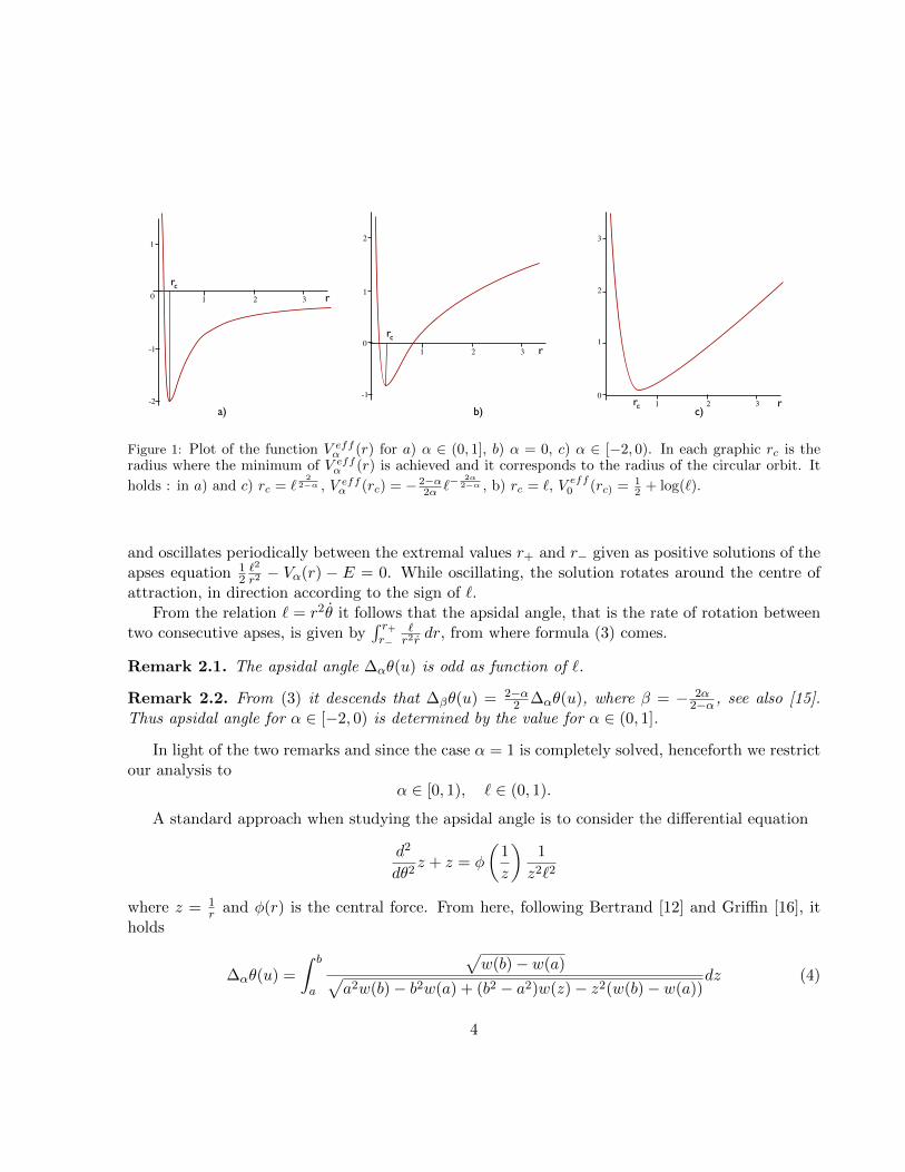
Figure 1: Plot of the function V effα (r) for a) α ∈ (0, 1], b) α = 0, c) α ∈ [−2, 0). In each graphic rc is theradius where the minimum of V effα (r) is achieved and it corresponds to the radius of the circular orbit. It

holds : in a) and c) rc = `2

2−α , V effα (rc) = − 2−α2α `−

2α2−α , b) rc = `, V eff0 (rc) = 1

2 + log(`).

and oscillates periodically between the extremal values r+ and r− given as positive solutions of theapses equation 1

2`2

r2− Vα(r) − E = 0. While oscillating, the solution rotates around the centre of

attraction, in direction according to the sign of `.From the relation ` = r2θ it follows that the apsidal angle, that is the rate of rotation between

two consecutive apses, is given by∫ r+r−

`r2r

dr, from where formula (3) comes.

Remark 2.1. The apsidal angle ∆αθ(u) is odd as function of `.

Remark 2.2. From (3) it descends that ∆βθ(u) = 2−α2 ∆αθ(u), where β = − 2α

2−α , see also [15].Thus apsidal angle for α ∈ [−2, 0) is determined by the value for α ∈ (0, 1].

In light of the two remarks and since the case α = 1 is completely solved, henceforth we restrictour analysis to

α ∈ [0, 1), ` ∈ (0, 1).

A standard approach when studying the apsidal angle is to consider the differential equation

d2

dθ2z + z = φ

(1

z

)1

z2`2

where z = 1r and φ(r) is the central force. From here, following Bertrand [12] and Griffin [16], it

holds

∆αθ(u) =

∫ b

a

√w(b)− w(a)√

a2w(b)− b2w(a) + (b2 − a2)w(z)− z2(w(b)− w(a))dz (4)

4

where the function w(z) = 2∫ψ(z) dz and ψ(z) = r2φ(r). In practice, for the force field we are

interest in, it holds

φ(r) = − 1

rα+1, ψ(z) = zα−1, w(z) =

2

αzα, α 6= 0

φ(r) = −1

r, ψ(z) = z−1, w(z) = 2 log(z), α = 0.

The dependence on ` and on the energy of the integral (4) is through the values of the a = 1/r+and b = 1/r−. Indeed, in the logarithmic potential case, such values are given as solutions of theequation log(z2)− `2z2 = −2E, whose roots can only be expressed as

z =

√−Wj(−`2e−2E)

`

where Wj represent the two branches of the Lambert W function, [17]. Similarly, in the homoge-neous case, a and b are the solutions of −`2z2 + 2

αzα = −2E.

From (4), by easy manipulation it follows

∆αθ(u) =

∫ b

a

dz√b2 − z2 − (b2 − a2)w(b)−w(z)w(b)−w(a)

=

∫ b

a

dz√(b− z)

((b+ z)− (b+ a)

w(b)−w(z)b−z

w(b)−w(a)b−a

)=

∫ b

a

1√z − a

1√b− z

1√1 + ε(z)

dz

where

ε(z) =b+ a

z − a

[1−

w(b)−w(z)b−z

w(b)−w(a)b−a

]. (5)

Let L := b− a and perform the change of variable s = z−aL ; it results

∆αθ(u) =

∫ 1

0

1√s(1− s)

1√1 + ε(s)

ds (6)

where

ε(s) =(2b− L)

Ls

[1−

w(b)− w(b− L(1− s)

)(1− s)

(w(b)− w(b− L)

)] .

Then, taking q = Lb , we obtain

∆αθ(u) =

∫ 1

0

1√s(1− s)

1√1 + Eα(s, q)

ds (7)

5

with

Eα(s, q) =2− qqs

[1−

1−(1− q(1− s)

)α(1− s)(1− (1− q)α)

], α ∈ (0, 1)

E0(s, q) =2− qqs

[1− log(1− q(1− s))

(1− s) log(1− q)

], α = 0

(8)

For any fixed value of the mechanical energy, the parameter q = 1 − ab is a function of the

angular momentum `. In particular, as ` increases from zero to `max, the ratio a/b increases from0 to 1. Therefore

q = q(`) ∈ (0, 1),dq

d`< 0, ∀` ∈ (0, 1).

The integral in (7) is the main object of investigation of the present paper. Two are the reasons whyit is advantageous to analyse (7) instead of the classical one (3): in the first integral the end-pointsare fixed and the dependence on the angular momentum is confined and well separated from thesingularities of the integrand function.

The behaviour of the apsidal angle as the angular momentum ` varies is intimately related tothe behaviour of the function Eα(q, s) when s, q vary in their domain. Hence, we first present adetailed analysis of the function Eα(s, q) and its derivative ∂qEα(s, q).

3. Analysis of the functions Eα(s, q)

It is convenient to introduce the weights

ωαn :=

−(αn

)(−1)n α ∈ (0, 1)

1n α = 0

∀n ≥ 1 (9)

and two auxiliary functions: for any n ≥ 2 let

An(s) :=1− (1− s)n−1

s, s ∈ (0, 1)

and, for any n ≥ 2 and α ∈ [0, 1) let

Kαn (s) := 2

ωαn+1

ωαnAn+1(s)−An(s) = 2

n− αn+ 1

An+1(s)−An(s), s ∈ (0, 1). (10)

Note that ωαn > 0 for any n ≥ 1 and α ∈ [0, 1). We collect in the Appendix all the properties ofthe functions An(s) and Kα

n (s) used throughout the paper.Recalling the power series expansions:

(1− x)α = 1 +∑n≥1

(α

n

)(−1)nxn, log(1− x) = −

∑n≥1

xn

n, |x| < 1

6

it holds, for α ∈ (0, 1),

Eα(s, q) =2− qqs

−(1− s)∑

n≥1(αn

)(−1)nqn +

∑n≥1

(αn

)(−1)nqn(1− s)n

(1− s)(−∑

n≥1(αn

)(−1)nqn

)

=2− q

qs(−∑

n≥1(αn

)(−1)nqn

)−∑

n≥2

(α

n

)(−1)nqn +

∑n≥2

(α

n

)(−1)nqn(1− s)n−1

=

1∑n≥1

(αn

)(−1)nqn−1

∑n≥2

(α

n

)(−1)nqn−2(2− q)An(s)

and similarly, for α = 0,

E0(s, q) =1∑

n≥11nq

n−1

∑n≥2

1

n(2− q)qn−2An(s).

By means of the weights ωαn , for any α ∈ [0, 1) we can write in compact form

Eα(s, q) =1∑

n≥1 ωαnq

n−1

∑n≥2

ωαn(2− q)qn−2An(s). (11)

Proposition 3.1. For any α ∈ [0, 1) and q ∈ (0, 1) the function Eα(q, s) is monotonically decreasingand convex in s for any s ∈ (0, 1).

Proof. Since A′2(s) = 0, for any α ∈ [0, 1)

d

dsEα(s, q) =

1∑n≥1 ω

αnq

n−1

∑n≥3

ωαnqn−2(2− q)A′n(s)

andd2

ds2Eα(s, q) =

1∑n≥1 ω

αnq

n−1

∑n≥4

ωαnqn−2(2− q)A′′n(s).

Since ωαn > 0 and, for point iii) of lemma 7.1, A′n < 0 and A′′n > 0, the thesis follows.�

Corollary 3.2. For any α ∈ [0, 1) the function Eα(s, q) > 0 for any s ∈ (0, 1), q ∈ (0, 1).

Proof. From the previous proposition

Eα(s, q) ≥ Eα(1, q) =

2−qq

(1−(1−q)α−αq

1−(1−q)α

), 0 < α < 1

2−qq

(1 + q

log(1−q)

), α = 0.

7

Since (1− q)α < 1− αq and − log(1− q) > q, it follows Eα(1, q) > 0 for any q ∈ (0, 1).�

Consider now the derivative of Eα(s, q) with respect to the variable q. For α ∈ [0, 1)

∂qEα(s, q) =1(∑

n≥1 ωαnq

n−1)2 ·

∑n≥2

ωαn

((n− 2)(2− q)− q

)qn−3An(s)

∑n≥1

ωαnqn−1

−

∑n≥2

ωαn(2− q)qn−2An(s)

∑n≥1

ωαn(n− 1)qn−2

=

1(∑n≥1 ω

αnq

n−1)2 · ∑

n≥2,m≥1ωαnω

αm

((2− q)(n−m)− 2

)An(s)q(n−2)+(m−2).

(12)

Henceforth, let us denote

Cα(q) :=

∑n≥1

ωαnqn−1

−2 .In the sequel we prove that the function ∂qEα(s, q) is monotonic and convex in s. For that let usintroduce the quantity

Hα(n,m) := ωαn+2ωαm(n−m)

and we prove the following.

Lemma 3.3. Let n,m ≥ 1 and n > m. Then, for any α ∈ [0, 1),

Hα(n,m) +Hα(m,n) > 0.

Proof. Case α = 0.

H0(n,m) +H0(m,n) =

(1

n+ 2

1

m− 1

m+ 2

1

n

)(n−m) = 2

(n−m)2

nm(n+ 2)(m+ 2)> 0.

Let be now α ∈ (0, 1). For any integer t, we remind the relations(α

t+ 1

)=α− tt+ 1

(α

t

),

(α

t+ 2

)=α− (t+ 1)

t+ 2

α− tt+ 1

(α

t

).

Then

Hα(n,m) +Hα(m,n) =

(α− (n+ 1)

n+ 2

α− nn+ 1

− α− (m+ 1)

m+ 2

α−mm+ 1

)ωαnω

αm(n−m)

=

((n+ 1)− α

n+ 2

n− αn+ 1

− (m+ 1)− αm+ 2

m− αm+ 1

)ωαnω

αm(n−m) .

(13)

Since K−αK+1 >

P−αP+1 > 0 whenever K > P ≥ 1, it follows Hα(n,m)+Hα(m,n) > 0 for any n > m. �

8

Proposition 3.4. For any α ∈ [0, 1) and q ∈ (0, 1)

i)d

ds

(∂qEα(s, q)

)< 0, ∀s ∈ (0, 1)

ii)d2

ds2

(∂qEα(s, q)

)> 0, ∀s ∈ (0, 1).

Proof. i) From (12), since A′2(s) = 0,

d

ds(∂qEα(s, q)) = Cα(q)

∑n≥3,m≥1

ωαnωαm

((2− q)(n−m)− 2

)A′n(s)q(n−2)+(m−2)

= Cα(q)∑p≥4

∑n+m=pn≥3,m≥1

ωαnωαm

((2− q)(n−m)− 2

)A′n(s)

qp−4.Denote

Coef(s, q, α, p) :=∑

n+m=pn≥3,m≥1

ωαnωαm

((2− q)(n−m)− 2

)A′n(s).

We prove that Coef(s, q, α, p) < 0 for any s ∈ (0, 1), q ∈ (0, 1) and α ∈ [0, 1) and p ≥ 4. Computefirst the derivative in q:

d

dqCoef(s, q, α, p) =−

∑n+m=pn≥3,m≥1

ωαnωαm(n−m)A′n(s).

For point iii) in lemma 7.1 A′n(s) < 0, then if p ≤ 6 the above sum is obviously positive, beingn ≥ m in any contribution. For p ≥ 7, we write

d

dqCoef(s, q, α, p) = −ωαp−1ωα1 (p−2)A′p−1(s)−ωαp−2ωα2 (p−4)A′p−2(s)−

∑n+m=pn≥3,m≥3

ωαnωαm(n−m)A′n(s).

The first and the second terms in the right hand side are positive then, collecting the contributionsto the sum due to the couples (n,m) and (m,n), and for point iv) in lemma 7.1, it holds

d

dqCoef(s, q, α, p) > −

∑n+m=pn>m≥3

ωαnωαm(n−m)(A′n(s)−A′m(s)) > 0.

9

Therefore, ddqCoef(s, q, α, p) > 0 for any p ≥ 4 and s ∈ (0, 1), q ∈ (0, 1), α ∈ [0, 1). It means that

Coef(s, q, α, p) < Coef(s, 1, α, p).

Now,

Coef(s, 1, α, p) =∑

n+m=pn≥3,m≥1

ωαnωαm

(n−m− 2

)A′n(s) =

∑n+m=p−2n≥1,m≥1

ωαn+2ωαm

(n−m

)A′n+2(s)

=∑

n+m=p−2n>m≥1

[ωαn+2ω

αm

(n−m

)A′n+2(s) + ωαm+2ω

αn

(m− n

)A′m+2(s)

].

Since ωαn+2ωαm > 0 and, again for property iii) of lemma 7.1, A′n+2(s) < A′m+2(s), it follows

Coef(s, 1, α, p) <∑

n+m=pn>m≥1

[ωαn+2ω

αm

(n−m

)+ ωαm+2ω

αn

(m− n

)]A′m+2(s)

=∑

n+m=pn>m≥1

(Hα(n,m) +Hα(m,n))A′m+2(s) < 0

in light of lemma 3.3. Therefore all the coefficients Coef(s, q, α, p) < 0 and dds (∂qEα(s, q)) < 0.

ii) Consider now the second derivative

d2

ds2

(∂qE(s, q)

)= Cα(q)

∑p≥5

∑n+m=pn≥4,m≥1

ωαnωαm

((2− q)(n−m)− 2

)A′′n(s)qp−4 .

Arguing as before, we realise that q = 1 represents the worst case and, since A′′n(s) > 0, it follows∑n+m=pn≥4,m≥1

ωαnωαm

((n−m)− 2

)A′′n(s) > 0, ∀s ∈ (0, 1), q ∈ (0, 1), α ∈ (0, 1), p ≥ 5.

�Up to now we investigated the monotonicity and the convexity of ∂qEα(q, s) without mentioning

the value of ∂qEα(q, s). To the purpose of proving the monotonicity of the apsidal angle, it wouldbe enough that ∂qEα(q, s) is positive for any s. Unfortunately that is not the case, indeed for any αthere is a region of q where ∂qEα(q, s) is not everywhere positive. Nevertheless, we prove now that∂qEα(q, s) > 0 at s = 1/2 for any α and q. For the previous result it follows that ∂qEα(q, s) > 0 forany s ∈ (0, 1/2), for any q and α.

10

Proposition 3.5. For any q ∈ (0, 1) and α ∈ [0, 1)

∂qEα(

1

2, q

)> 0.

Proof.

∂qEα(

1

2, q

)= Cα(q)

∑p≥3

∑n+m=pn≥2,m≥1

ωαnωαm

((2− q)(n−m)− 2

)An(1/2)qp−4

= Cα(q)∑p≥3

∑n+m=pn≥2,m≥1

ωαnωαm

(2(n−m− 1)

)An(1/2)qp−4

−∑

n+m=pn≥2,m≥1

ωαnωαm

(n−m

)An(1/2)qp−3

.When p = 3 the first sum does not contribute, then we can write

∂qEα(

1

2, q

)= Cα(q)

∑p≥4

∑n+m=pn≥2,m≥1

ωαnωαm2(n−m− 1)An(1/2)−

∑n+m=p−1n≥2,m≥1

ωαnωαm

(n−m

)An(1/2)

qp−4.Denote by

Qp(q) :=∑

n+m=pn≥2,m≥1

ωαnωαm2(n−m− 1)An(1/2)−

∑n+m=p−1n≥2,m≥1

ωαnωαm(n−m)An(1/2)

the coefficient of qp−4. For p ≥ 4

Qp(q) =∑

n+m=p−1n≥1,m≥1

ωαn+1ωαm2(n−m)An+1(1/2)−

∑n+m=p−1n≥2,m≥1

ωαnωαm(n−m)An(1/2)

= ωα2 ωαp−22(3− p)A2(1/2) +

∑n+m=p−1n≥2,m≥1

ωαnωαm(n−m)

(2ωαn+1

ωαnAn+1(1/2)−An(1/2)

)

= ωα2 ωαp−22(3− p)A2(1/2) + ωαp−2ω

α1 (p− 3)

(2ωαp−1ωαp−2

Ap−1(1/2)−Ap−2(1/2)

)

+∑

n+m=p−1n≥2,m≥2

ωαnωαm(n−m)

(2ωαn+1

ωαnAn+1(1/2)−An(1/2)

).

11

Reminding the definition (10) of Kαn (s) and collecting the contributions due to the couple (n,m)

and (m,n), it results

Qp(q) = ωαp−2(p− 3)

[2ωα1

ωαp−1ωαp−2

Ap−1(1/2)− ωα1Ap−2(1/2)− 2ωα2A2(1/2)

]+

∑n+m=p−1n>m≥2

ωαnωαm(n−m)

(Kαn (1/2)−Kα

m(1/2)).

For point ii) in lemma 7.2, the last sum is positive. Moreover, for α ∈ (0, 1), the function

ηα(p) := 2ωα1ωαp−1ωαp−2

Ap−1(1/2)− ωα1Ap−2(1/2)− 2ωα2A2(1/2)

=2α(p− 2− α)

p− 1Ap−1(1/2)− αAp−2(1/2)− α(1− α)

is such that

ηα(4) = 0, ηα(p) =2α(2 + 2α)

(p− 1)22p−2

(2p−2 − 1− (p− 1) log(2)

)> 0 ∀p ≥ 4.

A similar result holds for η0(p). Thus Qp(q) > 0 for any p ≥ 4 and α ∈ [0, 1) and the thesis follows.�

4. Limits of ∆αθ(u) as ` → 0 and ` → `max

This section concerns the limits of the apsidal angle for near-circular and near-radial orbits,that is when `→ `max and `→ 0.

Although these limit values are well known in the literature, we present the result for the sakeof completeness and because it descends directly from the above computations.

Theorem 4.1. For any α ∈ [0, 1)

lim`→0

∆αθ(u) =π

2− α, lim

`→`max

∆αθ(u) =π√

2− α.

Proof. According to the discussion in section 2, the limit values for the apsidal angle are given asthe limit for q → 0 and q → 1 of the integral (7). In particular, q → 0 corresponds to ` → `maxand q → 1 to `→ 0. Since Eα(s, q) > 0 for any α ∈ [0, 1), q ∈ (0, 1), s ∈ (0, 1), see Corollary 3.2, forthe Lebesgue’s dominated convergence theorem,

limq→0

∆αθ =

∫ 1

0

1√s(1− s)

1√1 + limq→0 Eα(s, q)

ds =

∫ 1

0

1√s(1− s)

1√1 + (1− α)

ds =π√

2− α

12

and

limq→1

∆αθ =

∫ 1

0

1√s(1− s)

1√1 + limq→1 Eα(s, q)

ds =

∫ 1

0

1√s(1− s)

1√1 + 1

ssα−s1−s

ds =π

2− α.

�

5. The derivative of ∆αθ(u)

We now examine the derivative of the apsidal angle as a function of the angular momentum`. That is equivalent to compute the derivative of ∆αθ(u) given in (7) with respect to q. FromProposition 3.4 and 3.5

|∂qEα(s, q)| < ∂qEα(0, q) = Mα(q)

whereMα(q) =

α2 (1− q)α q3 +(

(2− α) (1− q)2α +(−2α2 + α− 4

)(1− q)α + 2

)q2

+(−4 (1− q)2α + 8 (1− q)α − 4

)q + 2((1− q)α − 1)2

((1− q)α − 1)2 (q − 1)2 q2,α ∈ (0, 1)

q3 − log (1− q) q2 − 2 q2 + 2 (log (1− q))2 q2 − 4 (log (1− q))2 q + 2 (log (1− q))2

(log (1− q))2 q2 (1− 2 q + q2)α = 0

is C1((0, 1)) for any α. Therefore, for any q ∈ (0, 1) we can pass the derivative under the integralsign and write

d

dq∆αθ(u) =

∫ 1

0

1√s(1− s)

∂q

(1√

1 + Eα(s, q)

)ds = −1

2

∫ 1

0

1√s(1− s)

∂qEα(s, q)

(1 + Eα(s, q))32

ds. (14)

The following analysis aims at proving that the integral in (14) is positive for any q ∈ (0, 1) andα ∈ [0, 1). It would mean that the apsidal angle is monotonically increasing as a function of theangular momentum ` for any α ∈ [0, 1).

Denote

Iα(q) :=

∫ 1

0

1√s(1− s)

∂qEα(s, q)

(1 + Eα(s, q))32

ds.

Taking advantage from the symmetry in s, it holds

Iα(q) =

∫ 1/2

0

1√s(1− s)

(∂qEα(s, q)

(1 + Eα(s, q))32

+∂qEα(1− s, q)

(1 + Eα(1− s, q))32

)ds.

13

By Propositions 3.4, 3.5, the first term of the integrand is positive, but, as said earlier, ∂qEα(1−s, q)could be negative. A sufficient condition for Iα(q) > 0 is that

∂qEα(s, q)

(1 + Eα(s, q))32

> − ∂qEα(1− s, q)(1 + Eα(1− s, q))

32

, ∀s ∈ (0, 1/2). (15)

The convexity of ∂qEα(s, q) in the variable s implies that ∂qEα(s, q) > |∂qEα(1− s, q)| for anys ∈ (0, 1/2). On the other side, from Proposition 3.1, Eα(s, q) > Eα(1 − s, q) hence the validity of(15) cannot be achieved from the global behaviour of Eα and ∂qEα, rather it deserves a carefullyanalysis.

Consider the function

Iα(s, q) := ∂qEα(s, q) (1 + Eα(1− s, q))32 + ∂qEα(1− s, q) (1 + Eα(s, q))

32 .

Clearly, the statement Iα(s, q) > 0 for any s ∈ (0, 1/2) is equivalent to (15), then we aim at provingthat Iα(s, q) is positive. The next lemma allows to replace the power 3

2 by 2.

Lemma 5.1. Let A ≥ C > 0, B,D > 0. If

AB2 − CD2 > 0⇒ AB32 − CD

32 > 0.

Proof.

AB2 > CD2 ⇒ A34B

32 > C

34D

32 ⇒ AB

32 > C

34A

14D

32 > CD

32 .

�For those s where ∂qEα(q, 1 − s) ≥ 0 it holds Iα(s, q) > 0 and (15) is true. While for those s

where ∂qEα(q, 1− s) < 0 it holds ∂qEα(q, s) > −∂qEα(q, 1− s), then for the lemma, we can replacethe above function Iα(s, q) by

Iα(s, q) := ∂qEα(q, s) (1 + Eα(q, 1− s))2 + ∂qEα(q, 1− s) (1 + Eα(q, s))2 (16)

and we investigate whether the new defined Iα(s, q) is positive.From (12) it descends, for α ∈ (0, 1),

Iα(q, s) = Cα(q)∑

n≥2,m≥1ωαnω

αm

((2− q)(n−m)− 2

)[ An(s) (1 + Eα(1− s, q))2

+An(1− s) (1 + Eα(s, q))2

]q(n−2)+(m−2).

(17)

Algebraic manipulations lead to the expansion

Iα(s, q) = Cα(q)∑p≥4

Qα(p, s)qp−4 (18)

14

where

Qα(p, s) =∑

n≥2,m≥1n+m=p

ωαnωαm2(n−m− 1)

[An(s)

(1 + Eα(1− s, q)

)2+An(1− s)

(1 + Eα(s, q)

)2]

−∑

n≥2,m≥1n+m=p−1

ωαnωαm(n−m)

[An(s)

(1 + Eα(1− s, q)

)2+An(1− s)

(1 + Eα(s, q)

)2].

(19)

Note that the quantities in square brackets are positive and increasing in n and it can be provedthat both the sums appearing in Qα(p, s) are positive for any p ≥ 4. However, Qα(p, s) has nota definite sign as q ranges in (0, 1) then we cannot conclude about the sign of Iα(s, q) looking atthe sign of each of the Qα(p, s)’s. Therefore we have to extrapolate the dependence on q fromeach of the Eα(s, q) and Eα(1 − s, q). By substituting the expansion (11) in (17), straightforwardcomputations give

Iα(q, s) = C2α(q)

∑n≥2,m≥1k1,k2≥2

ωαnωαmω

αk1ω

αk2

((2− q)(n−m)− 2

)q(n−2)+(m−2)+(k1−2)+(k2−2)·

·

An(s)

(ωαk1−1

ωαk1+ (2− q)Ak1(1− s)

)(ωαk2−1

ωαk2+ (2− q)Ak2(1− s)

)+An(1− s)

(ωαk1−1

ωαk1+ (2− q)Ak1(s)

)(ωαk2−1

ωαk2+ (2− q)Ak2(s)

) .(20)

Note that in the series there is no the term q−1. Indeed the only possibility for this term to appearis for the choice (n,m, k1, k2) = (2, 1, 2, 2) but the first bracket results −q. Also the coefficient ofq0 is equal to zero. Therefore, collecting on the powers of q, we can write

Iα(q, s) = C2α(q)

∑p≥1

Coefp(α, s)qp

where, for any p, only a finite number of quart-uple (n,m, k1, k2) contributes to Coefp(α, s). Herewe list the first few of these coefficients, for the case α ∈ (0, 1).

Coef1(α, s) =1

9(2− α)2

((5 + α)s2α− (5 + α)s+ α+ 2

)Coef2(α, s) =

1

18α4(1− α)(7− 4α)(2− α)3

((5 + α)s2α− (5 + α)s+ α+ 2

)

15

Coef3(α, s) =1

90α4(2− α)3(1− α)

(α3 − 5α2 − 17α+ 69

)s4+(

10α2 − 138− 2α3 + 34α)s3+(

482− 346α+ 15α2 + 23α3)s2+(

−22α3 − 20α2 − 413 + 329α)s+

21α3 − 84α− 39α2 + 156

Coef4(α, s) =1

540α4(1− α)(2− α)3(9− 4α)

(3α3 − 15α2 − 51α+ 207

)s4+(

−6α3 + 30α2 + 102α− 414)s3+(

29α3 − 5α2 − 428α+ 746)s2+(

−26α3 − 10α2 + 377α− 539)s+

23α3 − 47α2 − 92α+ 188

.

The first two coefficients are clearly positive for any s ∈ (0, 1/2) and α ∈ (0, 1) and the same holds forCoef3(α, s), Coef4(α, s). By symbolic computation and numerical visualisation it appears evidentthat even for larger p the coefficients Coefp(α, s) are positive and, therefore, that Iα(q, s) > 0.On the other side, although rigorous, the check of the positivity of any large but finite number ofcoefficients does not provide a proof for Iα(q, s) > 0, unless a proof that Coefp(α, s) > 0 for anyp > p? is provided.

That is exactly what we are presenting in the next section, where the monotonicity of theapsidal angle is proved in the case α = 0.

6. The monotonicity of the apsidal angle in the logarithmic potential case

We aim at proving that, for any fixed value of the energy, the apsidal angle ∆0θ(u) is mono-tonically increasing as a function of the angular momentum `. According to the discussion of theprevious sections, it is enough to prove that the function

I0(s, q) = ∂qE0(s, q) (1 + E0(1− s, q))2 + ∂qE0(1− s, q) (1 + E0(s, q))2 (21)

is positive for any s ∈ (0, 1/2) and q ∈ (0, 1).The proof is split in different steps and analytical arguments are sometimes combined with rig-

orous numerical computations based on interval arithmetics, [18]. All the numerical computationshave been performed in Matlab with the interval arithmetic package Intlab. [19]. That assures thatthe results we obtain are reliable in the strict mathematical sense.

First we show that ∂qE0(1−s, q) > 0 for any s ∈ (0, 1/2) for any q ∈ [0.9, 1), yielding I0(s, q) > 0for any s ∈ (0, 1/2), q ∈ [0.9, 1).

Proposition 6.1. For any q ∈ [0.9, 1), s ∈ (0, 1/2), ∂qE0(1− s, q) > 0.

Proof. From Proposition 3.4, it is enough to show that lims→1 ∂qE0(s, q) > 0 for q ∈ [0.9, 1).It holds

F (q) := lims→1

∂qE0(s, q) = − 2

q2− 1

log(1− q)+

2− q(1− q) log2(1− q)

.

16

Compute

F ′(q) =4(1− q)2 log3(1− q) + q4 log(1− q) + 2q3(2− q)

q3(1− q)2 log3(1− q)=:

N(q)

D(q).

The denominator D(q) is negative for any q ∈ (0, 1), while the numerator

N(q) < −4(1− q)2q3 + q4 log(1− q) + 2q3(2− q) = q4(

log(1− q)− 4q + 6)

=: q4B(q).

The function B(q) is decreasing in q and, by rigorous computation it holds B(0.91) < −0.04.Moreover, for any q ∈ [0.9, 0.91] it holds N(q) < −0.2. Therefore N(q) < 0 and F (q) is increasingfor any q ∈ [0.9, 1). Since F (0.9) ∈ [0.0394, 0.040] it follows that F (q) > 0 for any q ∈ [0.9, 1).

�From now on, we restrict our analysis to the case q ∈ (0, 0.9]. For these values of q the function

∂qE0(1 − s, q) is not everywhere positive for s ∈ (0, 1/2) then the argument above adopted is notanymore valid to prove that I0(s, q) > 0.

From (18), we can separate

I0(s, q) = C0(q)(If0 (s, q) + I∞0 (s, q)

)= C0(q)

10∑p=4

Q0(s, p)qp−4 +

∑p≥11

Q0(s, p)qp

(22)

and we prove separately, in Section 6.1 and 6.2, that the series I∞0 (s, q) and the finite sum If0 (s, q)are positive for any s ∈ (0, 1/2) and q ∈ (0, 0.9]. Reminding the definition (19) and (9), for thelogarithmic potential case, we have

Q0(p, s) =∑

n≥2,m≥1n+m=p

1

n

1

m2(n−m− 1)

(An(s)

(1 + E0(1− s, q)

)2+An(1− s)

(1 + E0(s, q)

)2)

−∑

n≥2,m≥1n+m=p−1

1

n

1

m(n−m)

(An(s)

(1 + E0(1− s, q)

)2+An(1− s)

(1 + E0(s, q)

)2).

(23)

It is convenient to express the coefficients Q0(p, s) in a different way: by a change of index n→ n+1

17

in the first sum, it follows

Q0(p, s) =∑

n≥1,m≥1n+m=p−1

1

n+ 1

1

m2(n−m)

(An+1(s)

(1 + E0(1− s, q)

)2+An+1(1− s)

(1 + E0(s, q)

)2)

−∑

n≥2,m≥1n+m=p−1

1

n

1

m(n−m)

(An(s)

(1 + E0(1− s, q)

)2+An(1− s)

(1 + E0(s, q)

)2)

=1

2

1

p− 22(1− (p− 2))

(A2(s)

(1 + E0(1− s, q)

)2+A2(1− s)

(1 + E0(s, q)

)2)+

∑n≥2,m≥1n+m=p−1

1

n+ 1

1

m2(n−m)

(An+1(s)

(1 + E0(1− s, q)

)2+An+1(1− s)

(1 + E0(s, q)

)2)

−∑

n≥2,m≥1n+m=p−1

1

n

1

m(n−m)

(An(s)

(1 + E0(1− s, q)

)2+An(1− s)

(1 + E0(s, q)

)2).

Collecting all the contributions and reminding the definition (10) it results

Q0(p, s) =∑

n≥2,m≥1n+m=p−1

1

n

1

m(n−m)

[Kn(s)

(1 + E0(1− s, q)

)2+Kn(1− s)

(1 + E0(s, q)

)2]

− p− 3

p− 2

((1 + E0(1− s, q)

)2+(

1 + E0(s, q))2)

.

(24)

6.1. Analytical estimate of the tail elements

The goal of this section is to prove that Q0(s, p) ≥ 0 for any s ∈ (0, 1/2), q ∈ (0, 1) and p ≥ 11.That implies that I∞0 (s, q) ≥ 0 for any s ∈ (0, 1/2) and q ∈ (0, 1).

In practice, we are going to prove that∑n≥2,m≥1n+m=p−1

1

n

1

m(n−m)K0

n(s) >p− 3

p− 2, ∀p ≥ 11, s ∈ (0, 1).

The first estimate is the following:

Lemma 6.2. For any p ≥ 10∑n≥2,m≥1n+m=p−1

1

n

1

m(n−m)K0

n(s) ≥∑

n≥2,m≥1n+m=p−1

1

n

1

m(n−m)

n− 1

n+ 1, ∀s ∈ (0, 1).

18

Proof. Set

g(s) :=∑

n≥2,m≥1n+m=p−1

1

n

1

m(n−m)K0

n(s).

Assume p is odd, p = 2l + 1. Then

g(s) =2l−2∑n=l+1

(m=2l−n)

1

n

1

m(n−m)

(K0n(s)−K0

m(s))

+2l − 2

2l − 1K0

2l−1(s)

=

2l−3∑n=l+1

(m=2l−n)

1

n

1

m(n−m)

(K0n(s)−K0

m(s))

+2l − 2

2l − 1K0

2l−1(s) +l − 2

2l − 2

(K0

2l−2(s)−K02 (s)

).

Any term (K0n(s) −K0

m(s)) inside the series is such that m ≥ 3 and n ≥ m + 2. By adding andsubtracting equal terms, we obtain

K0n(s)−K0

m(s) =(K0n(s)−K0

n−1(s))

+(K0n−1(s)−K0

n−2(s))· · ·+

(K0m+1(s)−K0

m(s)), if m > 3

or

K0n(s)−K0

m(s) =(K0n(s)−K0

n−1(s))

+(K0n−1(s)−K0

n−2(s))· · ·+

(K0

5 (s)−K03 (s)

), if m = 3.

In both the cases, for point iii) of Proposition 7.2 and for Remark 7.3, we infer

K0n(s)−K0

m(s) ≥ K0n(1)−K0

m(1).

Again, for point i) of Proposition 7.2,

K02l−2(s) ≥ K0

2l−2(1)

and, for Lemma 7.4,

2l − 2

2l − 1K0

2l−1(s)−l − 2

2l − 2K0

2 (s) ≥ 2l − 2

2l − 1K0

2l−1(1)− l − 2

2l − 2K0

2 (1)

for any l ≥ 1.Therefore, collecting all these bounds, we conclude

g(s) ≥ g(1) =∑

n≥2,m≥1n+m=p−1

1

n

1

m(n−m)K0

n(1) =∑

n≥2,m≥1n+m=p−1

1

n

1

m(n−m)

[2n

n+ 1− 1

].

19

The case p even is completely equivalent. Indeed setting p = 2l + 2 we obtain

g(s) =2l−2∑n=l+1

(m=2l+1−n)

1

n

1

m(n−m)

(K0n(s)−K0

ms))

+2l − 3

2(2l − 1)K0

2l−1(s) +2l − 1

2lK0

2l(s)−2l − 3

2(2l − 1)K0

2 (s).

Note that when m = 3 then n = 2l−2 = p−4 ≥ 6, therefore the term K4(s)−K3(s) is not present.Arguing as before, we conclude that g(s) ≥ g(1).

�Define

S(p) :=∑

n≥2,m≥1n+m=p−1

1

n

1

m(n−m)

1

n+ 1.

Lemma 6.3. S(p) is decreasing for any p > 4 and S(p) < 0 for any p ≥ 11.

Proof.

S(p) =

p−2∑n=2

(1

p− 1− n− 1

n

)1

n+ 1.

Then

S(p)− S(p+ 1) =

p−2∑n=2

(1

p− 1− n− 1

n

)1

n+ 1−

p−1∑n=2

(1

p− n− 1

n

)1

n+ 1

=

p−2∑n=2

(1

p− 1− n− 1

p− n

)1

n+ 1−(

1− 1

p− 1

)1

p.

Since(

1p−1−n −

1p−n

)> 0 for any n = 2 . . . , p− 2, it holds

S(p)− S(p+ 1) ≥ 1

p− 1

p−2∑n=2

(1

p− 1− n− 1

p− n

)− p− 2

p(p− 1)

=1

p− 1

[p−1∑n=3

1

p− n−

p−2∑n=2

1

p− n

]− p− 2

p(p− 1)

=1

p− 1

(1− 1

p− 2

)− p− 2

p(p− 1)=

p− 4

(p− 2)(p− 1)p> 0 ∀p > 4.

Then S(p) is decreasing for any p > 4. In particular S(11) = − 291260 .

�We are now in the position to prove

20

Theorem 6.4. For any s ∈ (0, 1) and any p ≥ 11∑n≥2,m≥1n+m=p−1

1

n

1

m(n−m)K0

n(s) >p− 3

p− 2.

Proof. By Lemma 6.2, for any p ≥ 10∑n≥2,m≥1n+m=p−1

1

n

1

m(n−m)K0

n(s) ≥∑

n≥2,m≥1n+m=p−1

1

n

1

m(n−m)

n− 1

n+ 1=

∑n≥2,m≥1n+m=p−1

1

n

1

m(n−m)

(1− 2

n+ 1

)

=∑

n≥2,m≥1n+m=p−1

(1

m− 1

n

)− 2

∑n≥2,m≥1n+m=p−1

1

n

1

m(n−m)

1

n+ 1.

The first sum gives

∑n≥2,m≥1n+m=p−1

(1

m− 1

n

)=

p−2∑n=2

(1

p− 1− n− 1

n

)= 1− 1

p− 2+

p−3∑n=2

1

p− 1− n−

p−3∑n=2

1

n=p− 3

p− 2

then, by Lemma 6.3, the thesis follows. �

Corollary 6.5. For any s ∈ (0, 12 ] and p ≥ 11

Q0(p, s) ≥ 0.

Proof. From (24)

Q0(p, s) =

∑n≥2,m≥1n+m=p−1

1

n

1

m(n−m)K0

n(s)− p− 3

p− 2

(1 + E0(1− s, q))2

+

∑n≥2,m≥1n+m=p−1

1

n

1

m(n−m)K0

n(1− s)− p− 3

p− 2

(1 + E0(s, q))2.

(25)

By Theorem 6.4 both the terms are non-negative whenever p ≥ 11. �

21

6.2. Rigorous bound for the finite sum

We are now concerning the finite part in the splitting (22). We wish to prove that

If0 (s, q) =10∑p=4

Q0(p, s)qp−4 ≥ 0, ∀s ∈ (0, 1/2), q ∈ (0, 0.9].

By inserting Q0(p, s) in the form (23), it results

If0 (s, q)

If0 (s, q) =

10∑p=4

∑n≥2,m≥1n+m=p

1

n

1

m2(n−m− 1)An(s)−

∑n≥2,m≥1n+m=p−1

1

n

1

m(n−m)An(s)

qp−4(1 + E0(1− s, q))2

+10∑p=4

∑n≥2,m≥1n+m=p

1

n

1

m2(n−m− 1)An(1− s)−

∑n≥2,m≥1n+m=p−1

1

n

1

m(n−m)An(1− s)

qp−4(1 + E0(s, q))2

= R(s, q)(

1 + E0(1− s, q))2

+R(1− s, q)(

1 + E0(s, q))2

(26)

where

R(s, q) :=10∑p=4

∑n≥2,m≥1n+m=p

1

n

1

m2(n−m− 1)An(s)−

∑n≥2,m≥1n+m=p−1

1

n

1

m(n−m)An(s)

qp−4.If we perform all the computations, we obtain

R(s, q) =− 2

3s+

1

3+

(1− 7

3s+ s2

)q +

(349

180− 239

45s− 6

5s3 +

43

10s2)q2

+

(−94

15s3 +

31

10+

4

3s4 +

689

60s2 − 197

20s

)q3

+

(249

56− 4523

280s− 10

7s5 +

4093

168s2 − 823

42s3 +

173

21s4)q4

+

(3

2s6 +

3739

126s4 − 15367

630s+

3749

630− 29941

630s3 − 143

14s5 +

28313

630s2)q5

+

(95663

12600− 218681

6300s+

474889

6300s2 − 620681

6300s3 +

5125

63s4 − 10517

252s5 +

439

36s6 − 14

9s7)q6.

22

Note that the coefficient of q0 is odd in s = 1/2.

Theorem 6.6. For any s ∈ (0, 1/2) and q ∈ (0, 0.9]

If0 (s, q) > 0.

Proof. For any q ∈ (0, 1) the function E(s, q) is decreasing in s, that is E(1, q) ≤ E(s, q) ≤ E(0, q).We know that R(s, q) ≥ 0 for any q ∈ [0, 1] and s ∈ [0, 12 ] while it could be negative for larger

values of s. Therefore, If0 (s, q) > 0 for those s where R(1− s) is positive, otherwise

If0 (s, q) ≥ B(s, q) := R(s, q)(

1 + E(1, q))2

+R(1− s, q)(

1 + E(0, q))2. (27)

Hence, it is enough to prove that B(s, q) > 0. Since B(s, q) is made up a finite number of termsand s, q are within bounded intervals, the problem B(s, q) > 0 is, at least theoretically, well suitedto be solved by rigorous numerics. Let us first show that B(s, q) > 0 for any s ∈ (0, 1/2) andq ∈ (0, 0.1] then we address the case q ∈ [0.1, 0.9]. The reason for this further splitting is thatR(s, q) +R(1− s, q) = O(q), meaning B(s, q)→ 0 for any s when q → 0. This behaviour underliesan obstacle for a rigorous computational scheme to be completely successful: indeed any numericaltool based on interval arithmetics will definitely result a non-positive output when computingB(s, q) at small values of q. Therefore, the case when q is small deserves a particular treatment.

First computation: q ∈ [0, 1/10]Let us prove that B(s, q) ≥ 0 for any s ∈ [0, 1], q ∈ [0, 1

10 ]. We compute

E(1, q) := lims→1E(s, q) =

2

q− 1 +

2− qln(1− q)

E(0, q) := lims→0E(s, q) = 1− 2

q− 2− q

(1− q) ln(1− q).

Using the relation ln(1− x)−1 > −(q + q2

2 + q3

3 + q4

4 + q5

5

)−1it follows

E(1, q) > 1− 1

3q +

1

90q3 − 29

90q4, ∀q ∈ (0, 1).

Similarly,

E(0, q) < 1 +1

3q +

1

3q2 +

1

3

(58 + 87 q + 8 q2 + 15 q3 + 12 q4

)(1− q) (60 + 30 q + 20 q2 + 15 q3 + 12 q4)

q3

< 1 +1

3q +

1

3q2 + 0.4q3, ∀q ∈ [0, 0.1].

23

By inserting the above estimates into (27)

B(s, q) ≥ R(s, q)(

2− 1

3q +

1

90q3 − 29

90q4)2

+R(1− s, q)(

2 +1

3q +

1

3q2 + 0.4q3

)2, ∀q ∈ [0, 0.1].

As expected, the 0th order term in q vanishes. Let be introduced R(s, q), E(1, q), E(0, q) so that

R(s, q) =

(1

3− 2

3s

)+ qR(s, q)(

2− 1

3q +

1

90q3 − 29

90q4)2

= 4 + qE(1, q),(

2 +1

3q +

1

3q2 + 0.4q3

)2= 4 + qE(0, q).

It results

B(s, q) ≥ q

4(R(s, q) + R(1− s, q)

)+(13 −

23s) (E(1, q)− E(0, q)

)+q(R(s, q)E(1, q) + R(1− s, q)E(0, q)

) .For the choice ∆(s) = 0.02, ∆(q) = 0.01, define the intervals

sj := [(j − 1)∆(s), j∆s], j = 1, . . . , 25, qk := [(k − 1)∆q, k∆q], k = 1, . . . , 10

so that⋃j sj ⊃ [0, 1/2] and

⋃k qk ⊃ [0, 1/10], Then, for any j, k in their range, we compute using

interval arithmetics the quantities

M(j, k) =4(R(sj , qk) + R(1− sj , qk)

)+

(1

3− 2

3sj

)(E(1, qk)− E(0, qk)

)+ qk

(R(sj , qk)E(1, qk) + R(1− sj , qk)E(0, qk)

).

(28)

It results minj,k(min(M(j, k))) > 0.2744, proving that B(s, q) > 0 for any s ∈(

0, 12

), q ∈

(0, 1

10

].

Second computation, q ∈ [0.1, 0.9]We are now concerned with the remaining part, that is when q ∈ [ 1

10 ,910 ]. We rigorously

compute the lower bound for B(s, q), as given in (27), for s ∈ (0, 1), q ∈ [0.1, 0.9]. With the choiceof ∆s = 2 · 10−3 and ∆q = 2 · 10−4 it results that B(s, q) ≥ 0.0013.

�We can now state the theorem:

Theorem 6.7. For any value of the energy E, the apsidal angle ∆0θ(u) is monotonically increasingas a function of the angular momentum.

Proof. From proposition 6.1, corollary 6.5 and theorem 6.6 it follows that I0(s, q) > 0 for anys ∈ (0, 1) and q ∈ (0, 1). Then, for lemma 5.1, the derivative in (14) is negative for any q ∈ (0, 1).Since q = q(`) is decreasing, it follows that

d

d`∆0θ(u) > 0, ∀` ∈ (0, `max).

�

24

7. Appendix

This appendix is intended to collect all the technical results concerning the functions An(s) andKαn (s, q).

7.1. Properties of An(s)

An(s) =1− (1− s)n−1

s, n ≥ 2, s ∈ (0, 1)

Lemma 7.1.

i) A2(s) = 1, An(1) = 1 for any n ≥ 2.

ii) An+1(s)−An(s) = (1− s)n−1, An+1(1− s)−An(1− s) = s(n−1).

iii) For any n ≥ 3 and s ∈ (0, 1), An(s) is decreasing and convex, i.e. A′n(s) < 0 and A′′n(s) > 0.

iv) For any n > m, A′n(s) < A′m(s) for any s ∈ (0, 1).

Proof. i), ii) are obvious.iii)

d

dsAn(s) =

−1 + (1− s)n−1 + (n− 1)(1− s)(n−2)ss2

.

Looking at the numerator, say N(s), we see that N(0) = 0, N(1) = −1 and

N ′(s) = −(n− 1)(1− s)n−2 − (n− 1)(n− 2)(1− s)n−3s+ (n− 1)(1− s)(n−2) < 0

hence An(s) is decreasing.

d2

ds2An(s) =

2s− 2s(1− s)(n−1) − 2(n− 1)(1− s)n−2s2 − (n− 2)(n− 1)(1− s)n−3s3

s4

=2− 2(1− s)(n−1) − 2(n− 1)(1− s)n−2s− (n− 2)(n− 1)(1− s)n−3s2

s3.

Looking at the numerator, N(s), we note that N(0) = 0, N(1) = 2 and

N ′ = (n− 3)(n− 2)(n− 1)(1− s)n−3 > 0, s ∈ (0, 1)

hence An(s) is convex.

25

iv)

d

dnA′n(s) =

(1− s)n−1 log(1− s) + (1− s)n−2s+ (n− 1)(1− s)n−2s log(1− s)s2

=(1− s)(n−2)

s2(log(1− s)(1− s) + s+ (n− 1)s log(1− s))

=(1− s)(n−2)

s2(log(1− s) + s+ (n− 2)s log(1− s)) < 0.

�

7.2. Properties of Kαn (s)

Kαn (s) = 2

n− αn+ 1

An+1(s)−An(s), s ∈ (0, 1), α ∈ [0, 1), n ≥ 2.

Lemma 7.2. For any α ∈ [0, 1) and n ≥ 2:

i) Kαn (s) is decreasing and convex for any s ∈ (0, 1).

ii) Kαn+1(s)−Kα

n (s) > 0 for any s ∈ (0, 1).

For any α ∈ [0, 1) and n ≥ 4

iii) Kαn+1(s)−Kα

n (s) is decreasing for any s ∈ (0, 1).

Proof. i) By a direct computation the property is proved for n = 2, 3. Then,

Kαn (s) =

2(n− α)

n+ 1An+1(s)−

1− (1− s)n−1 + (1− s)n − (1− s)n

s

=

(2(n− α)

n+ 1− 1

)An+1(s) + (1− s)n−1,

(29)

hence

d

dsKαn (s) =

(n− 2α− 1

n+ 1

)A′n+1(s)− (n− 1)(1− s)n−2 < 0, ∀s ∈ (0, 1), n ≥ 4.

Also,

d2

ds2Kαn (s) =

(n− 2α− 1

n+ 1

)A′′n+1(s) + (n− 2)(n− 1)(1− s)n−3 > 0, ∀s ∈ (0, 1), n ≥ 4.

ii) The case n = 2 gives Kα3 (s)−Kα

2 (s) = 56 −

136 s+ 3

2 s2 − 1

6 a+ 56 αs−

12αs

2 that is positivefor any s ∈ (0, 1) and α ∈ [0, 1).

26

In the general case

Kαn+1(s)−Kα

n (s) =2(n+ 1− α)

n+ 2An+2(s)−

3n+ 1− 2α

n+ 1An+1(s) +An(s)

=1

(n+ 1)(n+ 2)[2(n+ 1)(n+ 1− α)An+2(s)− (3n+ 1− 2α)(n+ 2)An+1(s) + (n+ 1)(n+ 2)An(s)] .

Using twice property ii) of Lemma 7.1 we obtain

Kαn+1(s)−Kα

n (s) =1

(n+ 1)(n+ 2)·

[2(α+ 1)An(s) + 2(n+ 1)(n+ 1− α)(1− s)n − (n2 + 3n− 2α)(1− s)n−1

].

Denote ηαn(s) := 2(n + 1)(n + 1 − α)(1 − s)n − (n2 + 3n − 2α)(1 − s)n−1. Its derivative ηαn(s) =

(1− s)n−2((n2 + 3n− 2α)(n− 1)− 2n(n+ 1)(n+ 1−α)(1− s)) is zero for (1− s) = (n2+3n−2α)(n−1)2n(n+1)(n+1−α)

where it corresponds the minimum for ηαn(s). We infer

ηαn(s) ≥ 2(n+ 1)(n+ 1− α)(n2 + 3n− 2α)n(n− 1)n

(2n)n(n+ 1− α)n(n+ 1)n− (n2+3n−2α)n(n− 1)n−1

(2n)n−1(n+ 1− α)n−1(n+ 1)n−1

= − (n2 + 3n− 2α)n(n− 1)n−1

2n−1nn(n+ 1− α)n−1(n+ 1)n−1.

(30)

For any α ∈ [0, 1) we can uniformly bound

ηαn(s) ≥ η(n) := − (n2 + 3n)n(n− 1)n−1

2n−1nn(n)n−1(n+ 1)n−1= −(n+ 3)n(n− 1)n−1

(2n)n−1(n+ 1)n−1.

The last ratio is monotonically decreasing for n ≥ 1, and it equals 32 at n = 3. Therefore ηαn(s) ≥ −3

2for any s ∈ (0, 1) and n ≥ 3, α ∈ [0, 1). Since An(s) ≥ 1 for any n and s ∈ (0, 1), it follows

Kαn+1(s)−Kα

n (s) ≥ 1

(n+ 1)(n+ 2)

(2− 3

2

)> 0.

iii) The case n = 4, 5 is proved by a direct computation.For n ≥ 6

d

ds

(Kαn+1(s)−Kα

n (s))

=1

(n+ 1)(n+ 2)·[

(2 + α)A′n(s)− 2n(n+ 1)(n+ 1− α)(1− s)n−1 + (n− 1)(n2+3n− 2α)(1− s)n−2].

Denote ναn (s) := −2n(n+ 1)(n+ 1− α)(1− s)n−1 + (n− 1)(n2+3n− 2α)(1− s)n−2. Then, arguingas before, we prove that

maxs∈(0,1)

(ναn (s)) =(n− 2)n−2(n2 + 3n− 2α)n−1

(2n)n−2(n+ 1)n−2(n+ 1− α)n−2.

27

Therefore, for any α ∈ [0, 1),

ναn (s) ≤ ν(n) :=(n− 2)n−2(n2 + 3n)n−1

(2n)n−2(n+ 1)n−2(n)n−2=

(n− 2)n−2n(n+ 3)n−1

(2n)n−2(n+ 1)n−2.

The function ν(n) is decreasing in n and ν(6) < 2. Since A′n(s) ≤ −1 for any s and n, it followsthat Kα

n+1(s)−Kαn (s) is decreasing in s for any n ≥ 6.

�

Remark 7.3. Kα4 (s) −Kα

3 (s) is not decreasing in s ∈ (0, 1) and the minimum is not achieved ats = 1. However the function K0

5 (s)−K03 (s), for s ∈ [0, 1] attains the minimum at s = 1. Indeed

K05 (s)−K0

3 (s) =11

6− 43

6s+

67

6s2 − 22

3s3 +

5

3s4

and the function has a local minimum and a local maximum at s1, s2 respectively, where s1 ∈ I1 =[0.7230, 0.7233] and s2 ∈ I2 = [0.871, 0.872]. For any s ∈ I1, K0

5 (s) −K03 (s) ∈ [0.1672, 0.1785] >

16 = K0

5 (1)−K03 (1).

Lemma 7.4. For any n ≥ 2, the function

gn(s) :=n− 1

nK0n(s)− n− 3

2(n− 1)K0

2 (s)

is monotonically decreasing for any s ∈ [0, 1].

Proof.

gn(s) =n− 1

nK0n(s)− n− 3

2(n− 1)

(4

3A3(s)− 1

)then, since A′3(s) = −1,

gn(s) =n− 1

n

d

dsK0n(s) +

4

3

n− 3

2(n− 1).

For point i) of lemma 7.2, for any s ∈ (0, 1),

gn(s) ≤ −n− 1

n

(n− 1

n+ 1

)+

2(n− 3)

3(n− 1)=−3(n− 1)3 + 2n(n− 3)(n+ 1)

3n(n+ 1)(n− 1)< 0, ∀n ≥ 2.

�

8. Acknowledgements

This work was partially supported by Grant MTM 2011-24766 of the MICINN, Spain.

28

References

[1] J. Touma and S. Tremaine. A map for eccentric orbits in non-axisymmetric potentials. Mon.Not. R. Astron. Soc., 292:905–919, 1997.

[2] S. R. Valluri, P. A. Wiegert, J. Drozd, and M. Da Silva. A study of the orbits of the logarithmicpotential for galaxies. Mon. Not. R. Astron. Soc., 427(3):2392–2400, 2012.

[3] C. Quigg and Jonathan L. Rosner. Quarkonium level spacings. Phys. Lett., 71:153, 1977.

[4] R.H. Hooverman. Charged particle orbits in a logarithmic potential. J. Appl. Phys.,34(12):3505–3508, 1963.

[5] Paul Newton. The N -vortex problem. Analytical techniques. Number 145 in Applied Mathe-matical Sciences. Springer-Verlag, New York, 2001.

[6] Roberto Castelli, Francesco Paparella, and Alessandro Portaluri. Singular dynamics undera weak potential on a sphere. Nonlinear Differential Equations and Applications NoDEA,20(3):845–872, 2013.

[7] Roberto Castelli and Susanna Terracini. On the regularization of the collision solutions ofthe one-center problem with weak forces. Discr. Contin. Dyn. Syst. Ser. A, 31(4):1197–1218,2011.

[8] Giovanni Bellettini, Giorgio Fusco, and Giovanni Federico Gronchi. Regularization of thetwo-body problem via smoothing the potential. Comm. Pure Appl. Anal., 2:323–353, 2003.

[9] Richard McGehee. Double collisions for a classical particle system with nongravitational in-teractions. Comment. Math. Helvetici, 56:524–557, 1981.

[10] Susanna Terracini and Andrea Venturelli. Symmetric trajectories for the 2n-body problemwith equal masses. Archive for Rational Mechanics and Analysis, 184(3):465–493, 2007.

[11] S. R. Valluri, P. Yu, G. E. Smith, and P. A. Wiegert. An extension of newton’s apsidalprecession theorem. Mon. Not. R. Astron. Soc., 358(4):1273–1284, 2005.

[12] J. Bertrand. Theoreme relatif au movement d’un point attire vers un center fixe. Compt.Rend. Acad. Sci., 77:849–853, 1873.

[13] Edmund Taylor Whittaker. A Treatise on the Analytical Dynamics of Particles and RigidBodies, 4th Ed. Cambridge University Press, Cambridge, 1959.

[14] Filadelfo C. Santos, Vitorvani Soares, and Alexandre C. Tort. Determination of the apsidalangles and Bertrand’s theorem. Phys. Rev. E, 79(3):036605, 2009.

29

[15] Aaron K. Grant and Jonathan L. Rosner. Classical orbits in power-law potentials. Am. J.Phys, 62(4):310–315, 1994.

[16] F. L. Griffin. On the apsidal angle in central orbits. Bull. Amer. Math. Soc., 14(1):6–16, 1907.

[17] D. E. G. Hare D. J. Jeffrey Robert M. Corless, G. H. Gonnet and D. E. Knuth. On theLambert W function. Adv. Comput. Math., 5:329–359, 1996.

[18] Siegfried M. Rump. Verification methods: rigorous results using floating-point arithmetic.Acta Numer., 19:287–449, 2010.

[19] S.M. Rump. INTLAB - INTerval LABoratory. In Tibor Csendes, editor, Develop-ments in Reliable Computing, pages 77–104. Kluwer Academic Publishers, Dordrecht, 1999.http://www.ti3.tu-harburg.de/rump/.

30