Doubling measures, monotonicity, and quasiconformality
20
arXiv:math/0611110v2 [math.CA] 20 Dec 2006 DOUBLING MEASURES, MONOTONICITY, AND QUASICONFORMALITY LEONID V. KOVALEV, DIEGO MALDONADO, AND JANG-MEI WU Abstract. We construct quasiconformal mappings in Euclidean spaces by integration of a discontinuous kernel against doubling measures with suitable decay. The differentials of mappings that arise in this way satisfy an isotropic form of the doubling condition. We prove that this isotropic doubling condi- tion is satisfied by the distance functions of certain fractal sets. Finally, we construct an isotropic doubling measure that is not absolutely continuous with respect to the Lebesgue measure. 1. Introduction Given a nonatomic positive Radon measure μ on R, define an increasing function f μ (x)= x 0 dμ(z ), so that f ′ μ = μ in the sense of distributions. It is well-known that μ is doubling if and only if f μ is quasisymmetric. We extend this relation between doubling measures and quasisymmetric mappings to higher dimensions. Observe that f μ (x)= 1 2 R x − z |x − z | + z |z | dμ(z ). For a nonatomic Radon measure μ on R n , n ≥ 1, we define f μ : R n → R n by (1.1) f μ (x)= 1 2 R n x − z |x − z | + z |z | dμ(z ). where |·| is now interpreted as the Euclidean norm. When n ≥ 2 the integrand in (1.1) is not compactly supported with respect to z . The integral (1.1) converges provided that μ satisfies the decay condition (1.2) |z|>1 |z | −1 dμ(z ) < ∞. For 0 <γ<n, let I γ μ(x)= R n |x − z | γ−n dμ(z ) be the Riesz potential of μ of order γ . Condition (1.2) is equivalent to I n−1 μ being finite almost everywhere. Here and in the sequel the words “almost everywhere” or “a.e.” refer to the Lebesgue measure. A positive Radon measure μ on R n is called doubling if there is a constant C ≥ 1 such that μ(2B) ≤ Cμ(B) for every ball B ⊂ R n . Here 2B stands for the ball that has the same center as B and twice its radius. 2000 Mathematics Subject Classification. Primary 30C65. Secondary 28A75, 42A55, 47H05. L.V.K. was supported by an NSF Young Investigator award under grant DMS 0601926. J.-M.W. was supported by the NSF grant DMS 0400810. 1
-
Upload
independent -
Category
Documents
-
view
6 -
download
0
Transcript of Doubling measures, monotonicity, and quasiconformality

arX
iv:m
ath/
0611
110v
2 [
mat
h.C
A]
20
Dec
200
6
DOUBLING MEASURES, MONOTONICITY, AND
QUASICONFORMALITY
LEONID V. KOVALEV, DIEGO MALDONADO, AND JANG-MEI WU
Abstract. We construct quasiconformal mappings in Euclidean spaces byintegration of a discontinuous kernel against doubling measures with suitabledecay. The differentials of mappings that arise in this way satisfy an isotropicform of the doubling condition. We prove that this isotropic doubling condi-tion is satisfied by the distance functions of certain fractal sets. Finally, weconstruct an isotropic doubling measure that is not absolutely continuous withrespect to the Lebesgue measure.
1. Introduction
Given a nonatomic positive Radon measure µ on R, define an increasing functionfµ(x) =
∫ x
0 dµ(z), so that f ′µ = µ in the sense of distributions. It is well-known that
µ is doubling if and only if fµ is quasisymmetric. We extend this relation betweendoubling measures and quasisymmetric mappings to higher dimensions. Observethat
fµ(x) =1
2
∫
R
x − z
|x − z| +z
|z|
dµ(z).
For a nonatomic Radon measure µ on Rn, n ≥ 1, we define fµ : R
n → Rn by
(1.1) fµ(x) =1
2
∫
Rn
x − z
|x − z| +z
|z|
dµ(z).
where |·| is now interpreted as the Euclidean norm. When n ≥ 2 the integrandin (1.1) is not compactly supported with respect to z. The integral (1.1) convergesprovided that µ satisfies the decay condition
(1.2)
∫
|z|>1
|z|−1 dµ(z) < ∞.
For 0 < γ < n, let
Iγµ(x) =
∫
Rn
|x − z|γ−n dµ(z)
be the Riesz potential of µ of order γ. Condition (1.2) is equivalent to In−1µ beingfinite almost everywhere. Here and in the sequel the words “almost everywhere”or “a.e.” refer to the Lebesgue measure. A positive Radon measure µ on R
n iscalled doubling if there is a constant C ≥ 1 such that µ(2B) ≤ Cµ(B) for everyball B ⊂ R
n. Here 2B stands for the ball that has the same center as B and twiceits radius.
2000 Mathematics Subject Classification. Primary 30C65. Secondary 28A75, 42A55, 47H05.L.V.K. was supported by an NSF Young Investigator award under grant DMS 0601926.J.-M.W. was supported by the NSF grant DMS 0400810.
1

2 LEONID V. KOVALEV, DIEGO MALDONADO, AND JANG-MEI WU
Theorem 1.1. Let µ be a doubling measure on Rn that satisfies the decay condi-
tion (1.2). The mapping fµ defined by (1.1) is η-quasisymmetric with η dependingonly on the doubling constant of µ. Furthermore, fµ is δ-monotone and for a.e.x ∈ R
n
(1.3)1
12C3In−1µ(x) ≤ ‖Dfµ(x)‖ ≤ πIn−1µ(x),
where C is the doubling constant of µ.
Theorem 1.1 expands the class of weights that are known to be comparableto Jacobians of quasiconformal mappings. The quasiconformal Jacobian problemposed by David and Semmes in [9] asks for a characterization of all such weights(see also [4, 6, 7, 16, 18]). The authors of [6] point out that such a characterizationwould give a good idea of which metric spaces are bi-Lipschitz equivalent to R
n.A mapping f : R
n → Rn is called monotone if 〈F (x) − F (y), x − y〉 ≥ 0 for all
x, y ∈ Rn, where 〈·, ·〉 is the inner product [2, 27]. In other words, F is monotone if
the angle formed by the vectors F (x)− F (y) and x− y is at most π/2. A strongerversion of this condition, introduced by Sobolevskii in [19], requires the angle to bebounded by a constant less than π/2.
Definition 1.2. Let δ ∈ (0, 1]. A mapping F from a convex domain Ω ⊂ Rn into
Rn is called δ-monotone if for all x, y ∈ Ω
(1.4) 〈F (x) − F (y), x − y〉 ≥ δ|F (x) − F (y)||x − y|.Let Ω be a domain in R
n. An injective mapping f : Ω → Rn is called η-quasi-
symmetric if there is a homeomorphism η : [0,∞) → [0,∞) such that
(1.5)|f(x) − f(z)||f(y) − f(z)| ≤ η
( |x − z||y − z|
), z ∈ Ω, x, y ∈ Ω \ z.
In the case n ≥ 2, f is called K-quasiconformal if f ∈ W 1,nloc (Ω; Rn) and the operator
norm of the derivative Df satisfies ‖Df(x)‖n ≤ K detDf(x), a.e. in Ω for someK ≥ 1.
Every sense-preserving quasisymmetric mapping f : Rn → R
n, n ≥ 2, is qua-siconformal and vice versa ([12, Ch. 10], [24, p. 98]). The following result relatesδ-monotone and quasisymmetric mappings.
Theorem 1.3. [14, Theorem 4] Suppose that n ≥ 2 and f : Ω → Rn is a non-
constant δ-monotone mapping. If B is a closed ball such that 2B ⊂ Ω, then f isη-quasisymmetric on B with η depending only on δ.
Quasiconformality is known to be related to the doubling condition in severalways [5, 17, 20]. For example, if f : R
n → Rn is quasiconformal, then ‖Df‖n is a
doubling weight, and moreover an A∞ weight [10]. Consequently, ‖Df‖ is doublingas well. Since δ-monotonicity is a stronger property than quasiconformality, one canexpect that the differential of a δ-monotone mappings exhibits a stronger doublingbehavior. Our Theorem 1.5 confirms this. Before stating it, we observe that aRadon measure µ is doubling if and only if there exists a constant A such that
A−1 ≤ µ(Q1)
µ(Q2)≤ A
for any congruent cubes Q1 and Q2 with nonempty intersection. Recall that twosubsets of R
n are called congruent if there is an isometry of Rn that maps one of
them onto the other.
DOUBLING MEASURES, MONOTONICITY, AND QUASICONFORMALITY 3
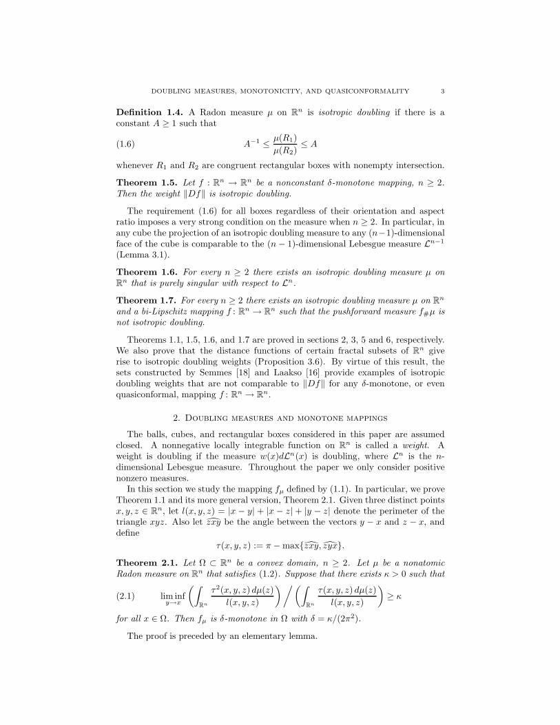
Definition 1.4. A Radon measure µ on Rn is isotropic doubling if there is a
constant A ≥ 1 such that
(1.6) A−1 ≤ µ(R1)
µ(R2)≤ A
whenever R1 and R2 are congruent rectangular boxes with nonempty intersection.
Theorem 1.5. Let f : Rn → R
n be a nonconstant δ-monotone mapping, n ≥ 2.Then the weight ‖Df‖ is isotropic doubling.
The requirement (1.6) for all boxes regardless of their orientation and aspectratio imposes a very strong condition on the measure when n ≥ 2. In particular, inany cube the projection of an isotropic doubling measure to any (n−1)-dimensionalface of the cube is comparable to the (n − 1)-dimensional Lebesgue measure Ln−1
(Lemma 3.1).
Theorem 1.6. For every n ≥ 2 there exists an isotropic doubling measure µ onR
n that is purely singular with respect to Ln.
Theorem 1.7. For every n ≥ 2 there exists an isotropic doubling measure µ on Rn
and a bi-Lipschitz mapping f : Rn → R
n such that the pushforward measure f#µ isnot isotropic doubling.
Theorems 1.1, 1.5, 1.6, and 1.7 are proved in sections 2, 3, 5 and 6, respectively.We also prove that the distance functions of certain fractal subsets of R
n giverise to isotropic doubling weights (Proposition 3.6). By virtue of this result, thesets constructed by Semmes [18] and Laakso [16] provide examples of isotropicdoubling weights that are not comparable to ‖Df‖ for any δ-monotone, or evenquasiconformal, mapping f : R
n → Rn.
2. Doubling measures and monotone mappings
The balls, cubes, and rectangular boxes considered in this paper are assumedclosed. A nonnegative locally integrable function on R
n is called a weight. Aweight is doubling if the measure w(x)dLn(x) is doubling, where Ln is the n-dimensional Lebesgue measure. Throughout the paper we only consider positivenonzero measures.
In this section we study the mapping fµ defined by (1.1). In particular, we proveTheorem 1.1 and its more general version, Theorem 2.1. Given three distinct pointsx, y, z ∈ R
n, let l(x, y, z) = |x − y| + |x − z| + |y − z| denote the perimeter of thetriangle xyz. Also let zxy be the angle between the vectors y − x and z − x, anddefine
τ(x, y, z) := π − maxzxy, zyx.
Theorem 2.1. Let Ω ⊂ Rn be a convex domain, n ≥ 2. Let µ be a nonatomic
Radon measure on Rn that satisfies (1.2). Suppose that there exists κ > 0 such that
(2.1) lim infy→x
(∫
Rn
τ2(x, y, z) dµ(z)
l(x, y, z)
)/(∫
Rn
τ(x, y, z) dµ(z)
l(x, y, z)
)≥ κ
for all x ∈ Ω. Then fµ is δ-monotone in Ω with δ = κ/(2π2).
The proof is preceded by an elementary lemma.

4 LEONID V. KOVALEV, DIEGO MALDONADO, AND JANG-MEI WU
Lemma 2.2. Fix z ∈ Rn and define gz(x) = (x − z)/|x− z| for x ∈ R
n \ z. Forany distinct points x, y ∈ R
n \ z we have
(2.2)2|x − y|
πl(x, y, z)τ(x, y, z) ≤ |gz(x) − gz(y)| ≤ 4|x − y|
l(x, y, z)τ(x, y, z)
and
(2.3)2|x − y|2
π2l(x, y, z)τ(x, y, z)2 ≤ 〈gz(x) − gz(y), x − y〉 ≤ 4|x − y|2
l(x, y, z)τ(x, y, z)2.
Proof. First we prove (2.2). By the sine theorem
(2.4)sin xzy
|x − y| =sin zyx + sin zxy
|x − z| + |y − z| .
Express the sum of sines as a product:
(2.5) sin zyx + sin zxy = 2 cosxzy
2cos
zyx − zxy
2.
Combining (2.4), (2.5), and the identity sin xzy = 2 sin dxzy2 cos dxzy
2 , we obtain
(2.6)sin dxzy
2
|x − y| =cos dzyx−dzxy
2
|x − z| + |y − z| .
The definition of gz implies
|gz(x) − gz(y)| = 2 sinxzy
2,
which together with (2.6) yield
(2.7) |gz(x) − gz(y)| =2|x − y|
|x − z| + |y − z| coszyx − zxy
2.
By the triangle inequality
(2.8)1
2l(x, y, z) ≤ |x − z| + |y − z| ≤ l(x, y, z).
Therefore (2.2) will follow from (2.7) once we prove that
(2.9)1
πτ(x, y, z) ≤ cos
zyx − zxy
2≤ τ(x, y, z).
Let α = maxzxy, zyx. We have
coszyx − zxy
2≥ cos
α
2= sin
π − α
2≥ 2
π
π − α
2=
1
πτ(x, y, z),
which proves the first inequality in (2.9). The second inequality is trivial whenα ≤ π/2, because then τ(x, y, z) = π − α > 1. If α > π/2, then
coszyx − zxy
2≤ cos
α − (π − α)
2= sin(π − α) ≤ π − α = τ(x, y, z).
This proves (2.9) and (2.2).

DOUBLING MEASURES, MONOTONICITY, AND QUASICONFORMALITY 5
The proof of (2.3) involves the identity cosα + cosβ = 2 cos α+β2 cos α−β
2 asfollows:
〈gz(x) − gz(y), x − y〉 =〈z − x, y − x〉
|x − z| +〈z − y, x − y〉
|y − z|= (cos zxy + cos xyz)|x − y|
= 2 sinxzy
2cos
zxy − xyz
2|x − y|
= |gz(x) − gz(y)||x − y| coszxy − xyz
2.
Applying (2.7) we obtain
(2.10) 〈gz(x) − gz(y), x − y〉 =2|x − y|2
|x − z| + |y − z| cos2zyx− zxy
2.
This together with (2.8) and (2.9) imply (2.3).
Proof of Theorem 2.1 . Since
fµ(x) − fµ(y) =1
2
∫
Rn
(gz(x) − gz(y)) dµ(z),
Lemma 2.2 implies the following inequalities.
(2.11) |fµ(x) − fµ(y)| ≤ 2|x − y|∫
Rn
τ(x, y, z)
l(x, y, z)dµ(z);
1
π2|x − y|2
∫
Rn
τ(x, y, z)2
l(x, y, z)dµ(z) ≤ 〈fµ(x) − fµ(y), x − y〉
≤ 2|x − y|2∫
Rn
τ(x, y, z)2
l(x, y, z)dµ(z).
(2.12)
Choose a number κ′ so that 0 < κ′ < κ. Combining (2.11), (2.12), and (2.1), weconclude that for every x ∈ Ω there exists ε(x) > 0 such that
(2.13) 〈fµ(x) − fµ(y), x − y〉 ≥ κ′
2π2|fµ(x) − fµ(y)||x − y|
whenever |x − y| ≤ ε(x). Next, let x and y be any distinct points in Ω. The linesegment [x, y] is covered by open balls B(z, ε(z)/2), z ∈ [x, y]. Choose a finitesubcover with centers zj = y + tj(x − y), 0 = t0 < t1 < · · · < tN = 1. Then
〈fµ(x) − fµ(y), x − y〉 =
N∑
j=1
〈fµ(zj) − fµ(zj−1), x − y〉
≥ κ′
2π2
N∑
j=1
|fµ(zj) − fµ(zj−1)||x − y|
≥ κ′
2π2|fµ(x) − fµ(y)||x − y|.
Letting κ′ → κ completes the proof.
Proof of Theorem 1.1. Let C be such that µ(2B) ≤ Cµ(B) for any ball B ⊂ Rn.
Given two distinct points x, y ∈ Rn and r > 0, choose a point w ∈ R
n so that x−wis orthogonal to x − y and |x − w| = r/2. It is easy to see that τ(x, y, z) ≥ π/3
6 LEONID V. KOVALEV, DIEGO MALDONADO, AND JANG-MEI WU
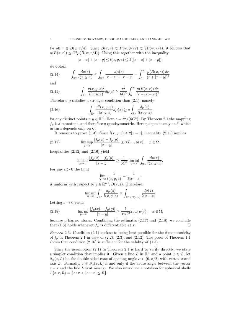
for all z ∈ B(w, r/4). Since B(x, r) ⊂ B(w, 3r/2) ⊂ 8B(w, r/4), it follows thatµ(B(x, r)) ≤ C3µ(B(w, r/4)). Using this together with the inequality
|x − z| + |x − y| ≤ l(x, y, z) ≤ 2(|x − z| + |x − y|),we obtain
(2.14)
∫
Rn
dµ(z)
l(x, y, z)≤∫
Rn
dµ(z)
|x − z|+ |x − y| =
∫ ∞
0
µ(B(x, r)) dr
(r + |x − y|)2and
(2.15)
∫
Rn
τ(x, y, z)2
l(x, y, z)dµ(z) ≥ π2
6C3
∫ ∞
0
µ(B(x, r)) dr
(r + |x − y|)2 .
Therefore, µ satisfies a stronger condition than (2.1), namely
(2.16)
∫
Rn
τ2(x, y, z)
l(x, y, z)dµ(z) ≥ c
∫
Rn
dµ(z)
l(x, y, z)
for any distinct points x, y ∈ Rn. Here c = π2/(6C3). By Theorem 2.1 the mapping
fµ is δ-monotone, and therefore η-quasisymmetric. Here η depends only on δ, whichin turn depends only on C.
It remains to prove (1.3). Since l(x, y, z) ≥ 2|x − z|, inequality (2.11) implies
(2.17) lim supy→x
|fµ(x) − fµ(y)||x − y| ≤ πIn−1µ(x), x ∈ Ω.
Inequalities (2.12) and (2.16) yield
lim infy→x
|fµ(x) − fµ(y)||x − y| ≥ 1
6C3lim inf
y→x
∫
Rn
dµ(z)
l(x, y, z).
For any ε > 0 the limit
limy→x
1
l(x, y, z)=
1
2|x − z|is uniform with respect to z ∈ R
n \ B(x, ε). Therefore,
lim infy→x
∫
Rn
dµ(z)
l(x, y, z)≥∫
Rn\B(x,ε)
dµ(z)
2|x − z|Letting ε → 0 yields
(2.18) lim infy→x
|fµ(x) − fµ(y)||x − y| ≥ 1
12C3In−1µ(x), x ∈ Ω,
because µ has no atoms. Combining the estimates (2.17) and (2.18), we concludethat (1.3) holds whenever fµ is differentiable at x.
Remark 2.3. Condition (2.1) is close to being best possible for the δ-monotonicityof fµ in Theorem 2.1 in view of (2.2), (2.3), and (2.12). The proof of Theorem 1.1shows that condition (2.16) is sufficient for the validity of (1.3).
Since the assumption (2.1) in Theorem 2.1 is hard to verify directly, we statea simpler condition that implies it. Given a line L in R
n and a point x ∈ L, letSα(x, L) be the double-sided cone of opening angle α ∈ (0, π/2) with vertex x andaxis L. Formally, z ∈ Sα(x, L) if and only if the acute angle between the vectorz − x and the line L is at most α. We also introduce a notation for spherical shellsA(x, r, R) = z : r < |z − x| ≤ R.

DOUBLING MEASURES, MONOTONICITY, AND QUASICONFORMALITY 7
Proposition 2.4. Let µ be a nonatomic Radon measure on Rn. Suppose that there
exist constants α ∈ (0, π/2), C > 0, and M ≥ 1 such that for any line L ⊂ Rn, any
x ∈ L and any r > 0 we have
(2.19) µ(A(x, r, 2r)) ≤ Cµ(A(x, M−1r, 2Mr) \ Sα(x, L)).
Then the measure µ satisfies (2.16) and consequently (2.1).
Proof. Without loss of generality we may assume that M = 2m for some integer m.Given y ∈ R
n \ x, let L be the line through x and y. Inequality (2.19) implies
(2.20)
∫
Rn
dµ(z)
l(x, y, z)≤ C1
∫
Rn\Sα(x,L)
dµ(z)
l(x, y, z)
where C1 depends only on C and M . Indeed,∫
Rn
dµ(z)
l(x, y, z)=∑
k∈Z
∫
A(x,2k,2k+1)
dµ(z)
l(x, y, z)≤∑
k∈Z
µ(A(x, 2k, 2k+1))
2k + |x − y|
≤ C∑
k∈Z
µ(A(x, M−12k, M2k+1) \ Sα(x, L))
2k + |x − y|
≤ C1
∫
Rn\Sα(x,L)
dµ(z)
l(x, y, z),
which proves (2.20). Since τ(x, y, z) ≥ α for all z /∈ Sα(x, L), estimate (2.20)implies (2.16).
Any doubling measure satisfies (2.19), because the set A(x, r, 2r) \Sα(x, L) con-tains a ball of radius comparable to r. The following result shows that (2.19) issatisfied by some non-doubling measures as well.
Proposition 2.5. Let ν be a doubling measure on Rn, n ≥ 2. Define a measure µ by
setting µ(E) = ν(E \B(0, 1)). Then µ satisfies the assumptions of Proposition 2.4.
Proof. Fix x ∈ Rn and r > 0. If A(x, r, 2r) ⊂ B(0, 1), then (2.19) holds. Suppose
that there is a point y ∈ A(x, r, 2r) \ B(0, 1). Let y′ = y + 4ry/|y|. Note thatB(y′, 2r)∩B(0, 1) = ∅ and 2r ≤ |y′−x| ≤ 6r. For every line L through x there is apoint z ∈ B(y′, r) such that dist(z, L) ≥ r. It follows that B(z, r/2)∩Sα(x, L) = ∅
for sufficiently small absolute constant α. Therefore,
B(z, r/2) ⊂ A(x, r/4, 8r) \ Sα(x, L).
Furthermore, µ(B(z, r/2)) = ν(B(z, r/2)) because B(z, r/2) ⊂ B(y′, 2r). Using thedoubling property of ν we obtain
ν(B(z, r/2)) ≥ C′ν(B(x, 2r)) ≥ µ(A(x, r, 2r))
where C′ depends on the doubling constant of ν.
Example 2.6. The measure µ defined by the weight
w(x) =
|x|p, |x| > 1,
0, |x| ≤ 1,
satisfies the assumptions of Theorem 2.1 whenever −n < p < 1 − n. However, µ isnot a doubling measure.
8 LEONID V. KOVALEV, DIEGO MALDONADO, AND JANG-MEI WU
Remark 2.7. For any γ ∈ (n−1, n) and every Radon measure µ the Riesz potentialIγµ is comparable to ‖Df‖ for some quasiconformal mapping f : R
n → Rn, pro-
vided that Iγµ(x) 6≡ ∞ [15, Lemma 4.1]. By the composition formula for Riesz po-tentials [21, p. 118] we have Iγµ = CIn−1Iγ−n+1µ for some constant C = C(n, γ).Since Iγ−n+1µ is a doubling measure, and even an A1-weight, Lemma 4.1 in [15]also follows from Theorem 1.1.
Remark 2.8. In [7] Bonk, Heinonen, and Saksman used quasiconformal flows to giveanother class of weights that are comparable to quasiconformal Jacobians. Theseare weights of the form
(2.21) w(x) = exp
−∫
Rn
log|x − z| dµ(z)
,
where µ is a signed Radon measure of sufficiently small total variation. Neither ofthe classes of weights in Theorem 1.1 and equation (2.21) is contained in the otherone.
It is possible that the relation between Riesz potentials and Jacobians of quasi-conformal mappings can be extended beyond the results presented here.
Question 2.9. Let n ≥ 2, 0 < γ < n, and let µ be a Radon measure on Rn such
that Iγµ 6≡ ∞. Does there exist a quasiconformal mapping f : Rn → R
n such thatC−1Iγµ ≤ detDf ≤ CIγµ a.e. for some constant C?
By Gehring’s theorem [10, Theorem 1] every quasiconformal mapping f on Rn
satisfies ‖Df‖ ∈ Lploc for some p > n. This and Theorem 1.1 immediately imply
the following result.
Corollary 2.10. If µ is a doubling measure on Rn, n ≥ 2, then the Riesz potential
In−1µ is either infinite at every point or is in Lploc(R
n) for some p > n.
Corollary 2.10 is probably known, although we could not find a reference.
3. Isotropic doubling measures
In this section we prove Theorem 1.5 and give several examples of isotropic dou-bling measures. It is clear that any weight w ∈ L∞(Rn) such that ess inf x∈Rn w(x) >0 is isotropic doubling.
Lemma 3.1. Suppose that a measure µ satisfies (1.6), and n ≥ 2. Then:
(i) For any congruent rectangular boxes R1, R2 ⊂ Rn
(3.1) A−m ≤ µ(R1)
µ(R2)≤ Am, where m =
⌈dist(R1, R2)
diam(R1)
⌉+ 1.
(ii) Let Q ⊂ Rn be a cube, and let F be a face of R. The pushforward π#µ|Q of
µ|Q under the orthogonal projection π : Q → F is comparable to Ln−1|F with
constants that depend only on n and A.
Proof. (i) There exist congruent boxes S0, . . . , Sm such that S0 = R1, Sm = R2,and Si ∩ Si−1 6= ∅ for i = 1, . . . , m. Repeated application of (1.6) yields (3.1).
(ii) Let l be the length of the edges of Q. Let Q1 and Q2 be congruent (n − 1)-dimensional cubes contained in F . The boxes Ri = π−1(Qi) have diameter at least

DOUBLING MEASURES, MONOTONICITY, AND QUASICONFORMALITY 9
l and the distance between them is at most diamF ≤√
n − 1l. By (3.1) we have
A−m ≤ π#µ(Q1)
π#µ(Q2)≤ Am, where m =
⌈√n − 1
⌉+ 1.
The statement follows by letting diam(Qi) → 0.
Lemma 3.1 implies that any isotropic doubling measure on Rn vanishes on sets
of (n − 1)-dimensional measure zero. The following lemma is the main step in ourproof of Theorem 1.5.
Lemma 3.2. Let f : Rn → R
n be a nonconstant δ-monotone mapping, n ≥ 2.There exists C > 1 such that for any rectangular box R ⊂ R
n
(3.2) C−1 diam(f(R))
diam(R)≤ 1
Ln(R)
∫
R
‖Df(x)‖dLn(x) ≤ Cdiam(f(R))
diam(R).
Here C depends only on δ and n.
Proof. Without loss of generality we may assume that
R = x : ∀i 0 ≤ xi ≤ ai, where a1 ≥ a2 ≥ · · · ≥ an.
We use e1, . . . , en to denote the standard basis vectors in Rn. Let π(x1, x2, . . . , xn) =
(0, x2, . . . , xn) be the orthogonal projection onto the linear span of e2, . . . , en. Fixz ∈ π(R) for now. Since f is quasisymmetric, it follows that
|f(z + a1e1) − f(z)| ≥ c diam f(R)
where c depends only on δ and n. On the other hand, Definition 1.2 implies that theimage of the line segment π−1(z)∩R under f is a rectifiable curve of length at mostδ−1|f(z + a1e1) − f(z)|, which is in turn bounded by δ−1 diam f(R). Therefore,
(3.3) c diam f(R) ≤∫ a1
0
‖Df(z + te1)‖ dt ≤ δ−1 diam f(R).
Integrating (3.3) over z ∈ π(R), we obtain
c diam f(R)
n∏
i=2
ai ≤∫
R
‖Df(x)‖ dLn(x) ≤ δ−1 diam f(R)
n∏
i=2
ai.
Dividing the latter inequality by Ln(R), we arrive at (3.2).
Proof of Theorem 1.5 . By virtue of Lemma 3.2 it suffices to prove that the ratiodiam f(R1)/ diam f(R2) is uniformly bounded for any congruent boxes R1 and R2
with R1 ∩ R2 6= ∅. Let d = diamR1 and pick a point y ∈ R1 ∩ R2. There existsz ∈ R2 such that |y − z| ≥ d/2. For any x ∈ R1 we have
|f(x) − f(y)||f(z)− f(y)| ≤ η
( |x − y||z − y|
)≤ η(2),
where η is the modulus of quasisymmetry of f . Therefore,
diam f(R1) ≤ 2η(2)|f(z) − f(y)| ≤ 2η(2) diam f(R2)
as required.

10 LEONID V. KOVALEV, DIEGO MALDONADO, AND JANG-MEI WU
Theorem 1.5 provides a large family of isotropic doubling weights. Indeed, forany set E ⊂ R
n of Hausdorff dimension dim E < 1 one can find a δ-monotonemapping f : R
n → Rn such that ‖Df‖ has essential limit 0 at every point of E (see
Theorem 5.6 [15] and Theorem 17 [14]).Let Q and R denote the sets of arbitrarily oriented cubes (resp. rectangular
boxes) of diameter at most 1. To a Radon measure µ on Rn we associate two
maximal functions
MQµ(x) = supµ(Q)/Ln(Q) : x ∈ Q ∈ Q;MRµ(x) = supµ(R)/Ln(R) : x ∈ R ∈ R.
Obviously MQµ(x) ≤ MRµ(x) for all x ∈ Rn.
Lemma 3.3. If µ is an isotropic doubling measure on Rn, then there exists C ≥ 1
such that MRµ(x) ≤ CMQµ(x) for all x ∈ Rn.
Proof. Fix x ∈ Rn. Given a box R ∈ R containing x, find a cube Q such that
R ⊂ Q, the edges of R and Q are parallel, and the edges of Q have the same lengthas a longest edge of R. Although in general Q /∈ Q, the diameter of Q cannotexceed
√n. Lemma 3.1 (ii) implies µ(R)/Ln(R) ≤ Cµ(Q)/Ln(Q). The doubling
property of µ and the definition of MQ yield µ(Q)/Ln(Q) ≤ CMQ(x).
Lemma 3.3 and [21, p. 5] imply that the maximal operator MR satisfies weak(1, 1) and strong (p, p) estimates when restricted to the linear span of isotropicdoubling weights with the same doubling constant. In [1, Theorem 1.4] the operatorMR was proved to be bounded on certain Besov spaces. Neither Lemma 3.3 norTheorem 1.4 [1] imply each other.
Example 3.4. The weight w(x) = |x|p, x ∈ Rn, is isotropic doubling if and only
if p > −1. Since the isotropic doubling condition is preserved under additionand weak∗ convergence of measures, for any Radon measure µ on R
n and anyγ ∈ (n − 1, n) the Riesz potential Iγµ is isotropic doubling unless Iγµ ≡ ∞.
Proof. Let µp be the measure |x|pdLn(x), and let
R1 = x ∈ Rn : |x1| ≤ 1; ∀i > 1 |xi| ≤ ε,
R2 = x ∈ Rn : |x1 − 2| ≤ 1; ∀i > 1 |xi − 1| ≤ ε.
If −n < p ≤ −1, then µp(R1)/εn−1 → ∞ as ε → 0. Indeed, |x| ≤ √nx1 whenever
x1 ≥ |xi| for all i > 1. The latter holds in particular when x ∈ R1 and x1 ≥ ε.Therefore,
µp(R1)
εn−1≥ np/2
∫ 1
ε
xp1dx1 → ∞, ε → 0.
Since µp(R2) ≤ 2nεn−1, by Lemma 3.1 (ii) the measure µp is not isotropic doublingin the range −n < p ≤ −1. The sufficiency part follows from Theorem 1.5. Indeed,for p > −1 the mapping fp(x) = |x|px is δ-monotone by Proposition 16 in [14]. ByTheorem 1.5 ‖Df‖ is an isotropic doubling weight. Since ‖Dfp‖ is a p-homogeneousradially symmetric function, it coincides with a constant multiple of |x|p.
Given two points a, b ∈ Rn, let [a, b] denote the segment λa+(1−λ)b : λ ∈ [0, 1].
A set A ⊂ Rn is uniformly linearly non-convex (ULNC) if there exists τ > 0 such
that the following holds: To each pair of distinct points a, b ∈ A there correspondsc ∈ [a, b] such that B(c, τ |a − b|) ∩ A = ∅. [25] The following lemma contains anequivalent definition of ULNC sets.

DOUBLING MEASURES, MONOTONICITY, AND QUASICONFORMALITY 11
Lemma 3.5. Suppose that A ⊂ Rn is ULNC with a constant τ > 0. Let τ ′ =
τ/(2+2τ). Then to each pair of distinct points a, b ∈ Rn there corresponds c ∈ [a, b]
such that B(c, τ ′|a − b|) ∩ A = ∅.
Proof. Without loss of generality we may assume that |a − b| = 1. Suppose thatthere are points a′, b′ ∈ A such that |a′ − a| ≤ τ ′ and |b′ − b| ≤ τ ′; otherwise wecan set c = a or c = b. Since |a′ − b′| ≥ (1 − 2τ ′), there exists c′ ∈ [a′, b′] suchthat B(c′, τ(1 − 2τ ′)) is disjoint from A. Each point of the segment [a′, b′] is atdistance at most τ ′ from a point of [a, b]. Therefore, there exists c ∈ [a, b] such that|c − c′| ≤ τ ′. The closed ball with center c and radius
τ(1 − 2τ ′) − τ ′ = τ
(1 − τ
1 + τ
)− τ
2 + 2τ=
τ
2 + 2τ= τ ′
is disjoint from A, as required.
Proposition 3.6. Let A ⊂ Rn be a nonempty ULNC set. Given p > 0, define
w(x) = dist(x, A)p for x ∈ Rn. The weight w is isotropic doubling.
The proof is preceded by a lemma.
Lemma 3.7. A continuous weight w ∈ C(Rn) is isotropic doubling if and only ifthere exists a constant C such that
(3.4)
∫ 1
0
w(x0 + tv) dt ≤ C
∫ 1
0
w(x0 + tv′) dt
for all points x0 ∈ Rn and all vectors v, v′ ∈ R
n such that |v| = |v′| > 0. Moreover,the constant A in (1.6) depends only on C in (3.4).
Proof. If w is continuous and isotropic doubling, then (3.4) follows by applying (1.6)to two thin rectangular boxes containing the segments x0 + tv : 0 ≤ t ≤ 1 andx0 + tv′ : 0 ≤ t ≤ 1. Conversely, suppose that (3.4) holds. Let R1 and R2 becongruent boxes with nonempty intersection. Let d be the length of a longest edgeof Ri. If Li ⊂ Ri is a segment of length d connecting two opposite faces of Ri, thenRi is contained in the closed
√n − 1d-neighborhood of Li for each i ∈ 1, 2. This
implies dist(L1, L2) ≤ 2√
n − 1d. For an integer N ≥ 2√
n − 1 + 2 we can find asequence of segments l1, . . . , lN of equal length such that l1 = L1, lN = L2, and lishares an endpoint with li+1 for i = 1, . . . , N − 1. A repeated application of (3.4)yields ∫
L1
w(x) ds ≤ CN−1
∫
L2
w(x) ds.
Since the box Ri is foliated by segments such as Li, inequality (1.6) holds withA = CN−1.
Proof of Proposition 3.6 . If dist(x0, A) ≥ 2|v|, then
dist(x0, A) ≤(∫ 1
0
w(x0 + tv) dt
)1/p
≤ 3 dist(x0, A).
If dist(x0, A) ≤ 2|v|, then
(∫ 1
0
w(x0 + tv) dt
)1/p
≤ 3|v|.

12 LEONID V. KOVALEV, DIEGO MALDONADO, AND JANG-MEI WU
Using Lemma 3.5 we obtain the reverse inequality
(∫ 1
0
w(x0 + tv) dt
)1/p
≥ c|v|,
where c > 0 depends only on τ in the definition of a ULNC set. By Lemma 3.7 theweight w is isotropic doubling.
Remark 3.8. Theorem 1.5 admits no converse, that is, there exist isotropicallydoubling weights that are not comparable to ‖Df‖ for any δ-monotone mappingf . This follows from the results of Semmes [18] and Laakso [16], who constructedcompact ULNC sets A ⊂ R
n such that for some p > 0 the weight w(x) := dist(x, A)p
is not comparable to ‖Df‖ for any quasiconformal mapping f : Rn → R
n. ByProposition 3.6 the weight w is isotropic doubling. The example of Semmes is aform of the Antoine’s necklace, and requires n ≥ 3 (see the proof of Theorem 1.10in [18]). The example of Laakso is two-dimensional [16, Theorem 1.7]. The fact thatthe sets considered by Semmes and Laakso are ULNC follows from Theorem 3.3in [25].
Remark 3.9. Buckley, Hanson and MacManus considered several stronger versionsof the doubling condition in [8], but our Definition 1.4 does not appear to be directlyrelated to any of them.
4. The Monge-Ampere measures
The main purpose of this section is to point out a consequence of Theorem 1.5for convex functions on R
n. Let u : Rn → R be a convex function, n ≥ 1. The
subdifferential of u at a point z ∈ Rn is the set
∂u(z) = p ∈ Rn : u(x) ≥ u(z) + 〈p, x − z〉 ∀x ∈ R
n.The convexity of u implies ∂u(z) 6= ∅ for all x ∈ R
n. The function u is differentiableat z ∈ R
n if and only if ∂u(z) is the one-point set ∇u(z). Given z ∈ Rn and
p ∈ ∂u(z), let
uz,p(x) = u(x) − u(z) − 〈p, x − z〉, x ∈ Rn.
The section [11, p. 45] of u with the center z ∈ Rn, direction p ∈ ∂u(z), and height
t > 0 is defined as
Su(z, p, t) = x ∈ Rn : uz,p(x) < t.
If u is Gateaux differentiable at z, then we write uz instead of uz,∇u(z). TheMonge-Ampere measure associated with u is defined by µu(E) = Ln(∂u(E)) forevery Borel set E ⊂ R
n. Note that adding an affine function to u does not changeµu. If u ∈ C2, then µu is absolutely continuous with the density detD2u(x), whereD2u is the Hessian matrix of u.
Definition 4.1. [15] A convex function u : Rn → R has round sections if there
exists a constant τ ∈ (0, 1) such that for every z ∈ Rn, p ∈ ∂u(z) and t > 0
(4.1) B(z, τR) ⊂ Su(z, p, t) ⊂ B(z, R)
for some R ∈ (0,∞).
Proposition 4.2. If a convex function u : Rn → R has round sections, then ||D2u||
is an isotropic doubling weight.

DOUBLING MEASURES, MONOTONICITY, AND QUASICONFORMALITY 13
Proof. First, consider the case n = 1. By Theorem 3.1 [15] and Remark 3.3 [15]u is continuously differentiable and ∇u : R → R is quasisymmetric. If I and J areadjacent intervals of equal length, then µu(I) ≤ η(1)µu(J), where η is as in 1.5.Thus µu is doubling, which in one dimension is the same as being isotropic doubling.
Next, assume n ≥ 2. By Theorem 3.1 [15] u is continuously differentiable, and thegradient mapping ∇u : R
n → Rn is quasiconformal. Since the change of variables
formula applies to quasiconformal mappings [26, Theorem 33.3], we have
µu(E) =
∫
E
detD2u(x) dLn(x), E ⊂ Rn measurable.
Quasiconformality also implies that detD2u is comparable to ‖D2u‖n up to a mul-tiplicative constant. By Theorem 14 [14] the gradient ∇u is a δ-monotone mapping,hence ‖D2u‖ is isotropic doubling by Theorem 1.5.
Remark 4.3. The mapping fµ defined by (1.1) is the gradient of the convex function
(4.2) vµ(x) :=
∫
Rn
|x − z| − |z| + 〈x, z〉
|z|
dµ(z).
Indeed, for all x, z ∈ Rn
x − z
|x − z| +z
|z| ∈ ∂
(|x − z| − |z| + 〈x, z〉
|z|
),
where the subgradient is taken with respect to x. Therefore, fµ(x) ∈ ∂vµ(x) for allx ∈ R
n. The continuity of fµ implies that vµ(x) is differentiable and ∇vµ = fµ.
If the gradient of a convex function is quasisymmetric, then it is δ-monotone byLemma 13 in [14]. This together with Remarks 2.3 and 4.3 indicate that condi-tion (2.1) is close to being best possible for the quasiconformality of fµ in Theo-rem 2.1.
5. Singular isotropic doubling measures
It is well-known that doubling measures on Rn can be supported on sets of
arbitrarily small positive Hausdorff measure ([3] and [22, p. 40]). This is not truefor isotropic doubling measures in dimensions n ≥ 2 by Lemma 3.1 (ii). In thissection we prove Theorem 1.6, which shows that isotropic doubling measures canbe singular with respect to Ln. We will use the following notation: #A is thecardinality of a finite set A, a ∨ b = maxa, b, a ∧ b = mina, b.Proof of Theorem 1.6 . Let us introduce a sequence of vectors
wk := 4nk2
(4k, 42k, 43k, . . . , 4nk) ∈ Rn, k = 1, 2, . . . .
For k ≥ 1 define
λk(x) = 1 +1
2cos(〈x, wk〉), x ∈ R
n.
and
Λm(x) =
m∏
k=1
λk(x).
We shall obtain a singular isotropic doubling measure µ as the weak∗ limit of asubsequence of Λm(x)dLn(x) : m ≥ 1. The proof involves several steps.
Step 1. Existence of µ. For each m the weight Λm is 2π-periodic in all vari-ables. Let Q = [−π, π]n. Clearly
∫Q Λ1(x) dLn(x) = (2π)n. For m ≥ 2 we obtain

14 LEONID V. KOVALEV, DIEGO MALDONADO, AND JANG-MEI WU
∫Q
(Λm − Λm−1)dLn = 0 by integrating in xn over the interval [−π, π] and using
the orthogonality of the trigonometric family. Therefore,∫
QΛm dLn = (2π)n for
all m ≥ 1. Choose a subsequence of Λm(x) dLn(x) converging in the weak∗ senseto a (2π)-periodic measure µ with µ(Q) = (2π)n.
Step 2. Lipschitz estimates. Since the Euclidean norm of wk satisfies
(5.1) 4n(k2+k) ≤ |wk| ≤ 2 · 4n(k2+k),
λk is a Lipschitz function with the constant Lk := 4n(k2+k). Therefore, for anyx, x′ ∈ R
n we have
(5.2)λk(x′)
λk(x)≥ 1/2
1/2 + Lk|x − x′| ≥ 1 − 2Lk|x − x′|.
Multiplying (5.2) over k = 1, . . . , m yields
(5.3)Λm(x′)
Λm(x)≥
m∏
k=1
(1 − 2Lk|x − x′|) ≥ 1 − 2|x − x′|m∑
k=1
Lk ≥ 1 − 3Lm|x − x′|
provided that 3Lm|x − x′| < 1. Thus
(5.4) 1 − 3Lm|x − x′| ≤ Λm(x′)
Λm(x)≤ (1 − 3Lm|x − x′|)−1, |x − x′| <
1
3Lm.
Step 3. Singularity of µ. Given x ∈ Rn and r > 0, let Q(x, r) denote the cube
y ∈ Rn : ∀i |xi − yi| ≤ r. To prove that µ is purely singular, it suffices to show
that
(5.5) lim infr→0
r−nµ(Q(x, r)) = 0 for a.e. x ∈ Rn.
For a.e. x ∈ Rn we have limm→∞ Λm(x) = 0 by [28, p. 209]. Fix such a point x. For
m ≥ 1 let rm = 4−n(m+1)2π. Note that the functions λk, k > m, are 2rm-periodicin each variable. Using orthogonality as in Step 1, we obtain
µ(Q(x, rm)) =
∫
Q(x,rm)
Λm(x) dLn(x).
For every y ∈ Q(x, rm) we have
3Lm|x − y| ≤ 3 · 4n(m2+m)√n4−n(m+1)2π → 0 as m → ∞.
Therefore, supΛm(y) : y ∈ Q(x, rm) → 0 as m → ∞. This proves (5.5).It remains to prove that Λm satisfies (1.6) with a constant independent of m.
Consider a segment L given by the parametric equations x = x0 + tv, 0 ≤ t ≤ 1,
of length r = ‖v‖ > 0. Set K = maxk ≥ 1: 4nk2 ≤ 1/r or K = 0 if no such kexists. Our goal is to show that
(5.6)
∫
L
Λm ds ≈n
r
K∧m∏
k=1
(1 +
1
2cos(〈x0, w
k〉))
where ≈n
indicates that multiplicative constants in the estimate depend only on n.
The estimate (5.6) implies (1.6) by Lemma 3.7.Step 4. Low-frequency terms. If K ≥ 2, then the terms λk with 1 ≤ k ≤ K − 1
are essentially constant on L. Indeed, (5.1) implies
(5.7) |〈v, wk〉| ≤ 2r4n(k2+k) ≤ 2 · 4−nK .

DOUBLING MEASURES, MONOTONICITY, AND QUASICONFORMALITY 15
This implies that for all 0 ≤ t ≤ 1 and all 1 ≤ k ≤ K − 1 we have
|λk(x0 + tv) − λk(x0)| ≤ 4−nK ,
hence
1 − 2 · 4−nK ≤ λk(x0 + tv)
λk(x0)≤ 1 + 2 · 4−nK .
Taking a product over k = 1, . . . , K − 1 yields
(5.8) (1 − 2 · 4−nK)K−1 ≤K−1∏
k=1
λk(x0 + tv)
λk(x0)≤ (1 + 2 · 4−nK)K−1.
Since
(1 − 2 · 4−nK)K−1 ≥ 1 − 2(K − 1)4−nK ≥ 1
2and
(1 + 2 · 4−nK)K−1 ≤ (1 − 2 · 4−nK)1−K ≤ 2,
inequality (5.8) implies
1
2
∫
L
Λm ds ≤ r
m∧(K−1)∏
k=1
(1 +
1
2cos(〈x0, w
k〉))
×∫ 1
0
m∏
k=m∧(K−1)
(1 +
1
2cos(〈x0 + tv, wk〉)
)dt ≤ 2
∫
L
Λm ds.
(5.9)
The estimate (5.9) proves (5.6) in the case m ≤ K + 1.Step 5. High-frequency terms. For the rest of the proof we assume m ≥ K + 2.
Let v∗ = (|v1|, |v2|, . . . , |vn|) be the vector whose components are the absolute valuesof the components of v. Introduce two sets of integers depending on v:
G =
K + 2 ≤ k ≤ m : |〈v, wk〉| ≥ 1
4〈v∗, wk〉
;
B = K + 2 ≤ k ≤ m : k /∈ G .
For every k ∈ G the restriction of λk to L is rapidly oscillating, because
(5.10) |〈v, wk〉| ≥ 4nk2−1n∑
i=1
4ik|vi| ≥ 4nk2+k−1|v| ≥ 4nk2+k−14−n(K+1)2 ≥ 4nk.
Furthermore, if k ∈ G and k > l ≥ 1, then the restriction of λk to L has period atleast 4nk times smaller than the period of the restriction of λl:
(5.11) |〈v, wk〉| ≥ 4nk2−1n∑
i=1
4ik|vi| ≥ 4n(k2−l2)−1n∑
i=1
4nl2+il|vi| ≥ 4nk|〈v, wl〉|.
We have chosen the vectors wk so that #B is bounded by a constant dependingonly on n, by Lemma 5.2 below. Hence
(5.12)
m∏
k=K
λk(x) ≈n
∏
k∈G
λk(x), x ∈ Rn.
Observe that
(5.13)∏
k∈G
(1 +
1
2cos(〈x0 + tv, wk〉)
)= 1+
∑
A⊆G, A 6=∅
1
2#A
∏
k∈A
cos(〈x0+tv, wk〉).

16 LEONID V. KOVALEV, DIEGO MALDONADO, AND JANG-MEI WU
Converting the trigonometric product into a sum, we obtain
∏
k∈A
cos(〈x0 + tv, wk〉) =1
2#A
∑
±
cos
(∑
k∈A
±〈x0 + tv, wk〉)
,
where the exterior sum is taken over all 2#A choices of the ± signs. Using (5.11),we find that for any choice of the signs
∣∣∣∣∣∑
k∈A
±〈v, wk〉∣∣∣∣∣ ≥
2
3|〈v, wmax A〉|,
where maxA is the maximal element of A. Therefore,∣∣∣∣∣
∫ 1
0
∏
k∈A
cos(〈x0 + tv, wk〉) dt
∣∣∣∣∣ ≤ 3|〈v, wmax A〉|−1 ≤ 3 · 4−n max A,
where the last inequality follows from (5.10). For any l ∈ G there exist at most2l−K−2 nonempty subsets A ⊆ G such that maxA = l. Thus we can estimate therighthand side of (5.13) as follows.
∑
A⊆G, A 6=∅
1
2#A
∣∣∣∣∣
∫ 1
0
∏
k∈A
cos(〈x0 + tv, wk〉) dt
∣∣∣∣∣ ≤ 3
m∑
l=K+2
4−nl2l−K−2
≤ 3∞∑
l=K+2
4−l = 4−K−1 ≤ 1
4.
(5.14)
Combining (5.13) and (5.14) yields
3
4≤∫ 1
0
∏
k∈G
(1 +
1
2cos(〈x0 + tv, wk〉)
)dt ≤ 5
4,
which together with (5.9) and (5.12) imply
(5.15)
∫
L
Λm ds ≈n
r
K∏
k=1
(1 +
1
2cos(〈x0, w
k〉))
.
This proves (5.6), and thereby the theorem.
Remark 5.1. The above construction is not symmetric with respect to the variablesx1, . . . , xn. This feature of µ will be used to prove Theorem 1.7. But one canconstruct a more symmetric singular measure ν =
∑σ T σ
#µ, where T σ(x1, . . . , xn) =
(xσ(1), . . . , xσ(n)) and the summation is over all permutations of n elements. Theisotropic doubling condition is obviously preserved under addition of measures.
Now we prove Lemma 5.2, which was used in Step 5 of the proof of Theorem 1.6with parameters q = 4 and ε = 3/4.
Lemma 5.2. Let (v1, . . . , vn) be a nonzero vector in Rn, where n ≥ 2. Given q > 1
and ε ∈ (0, 1), define
B(q, ε) =
k ∈ Z :
∣∣∣∣∣n∑
i=1
qikvi
∣∣∣∣∣ <1 − ε
1 + ε
n∑
i=1
qik|vi|
.

DOUBLING MEASURES, MONOTONICITY, AND QUASICONFORMALITY 17
Then
(5.16) #B(q, ε) ≤ n(n − 1)log((n − 1)/ε)
log q.
Proof. We claim that
(5.17) B(q, ε) ⊆⋃
1≤i<j≤n
Aij ,
where
Aij =
k ∈ Z :
ε
n − 1≤ qik|vi|
qjk|vj |≤ n − 1
ε
if vj 6= 0 and Aij = ∅ otherwise. Indeed, suppose that k ∈ Z \⋃1≤i<j≤n Aij . Let
m be such that qik|vi| is maximal when i = m. Then∣∣∣∣∣
n∑
i=1
qikvi
∣∣∣∣∣ ≥ qmk|vm| −∑
i6=m
qik|vi| ≥ (1 − ε)qmk|vm|,
while on the other handn∑
i=1
qik|vi| ≤ qmk|vm| + (n − 1)ε
n − 1qmk|vm| = (1 + ε)qmk|vm|.
Thus k 6= B(q, ε), which proves (5.17). It remains to estimate the cardinality of thesets Aij , 1 ≤ i < j ≤ n. We may assume that vj 6= 0, for otherwise Aij is empty.Since
Aij =
k ∈ Z : log
ε
n − 1≤ k(i − j) log q + log
|vi||vj |
≤ logn − 1
ε
,
it follows that
#Aij ≤ 2 log((n − 1)/ε)
|i − j| log q≤ 2 log((n − 1)/ε)
log q,
which after summation yields (5.16).
Question 5.3. Is it true that every isotropic doubling measure on Rn is absolutely
continuous with respect to the s-dimensional Hausdorff measure for all s < n?
Lemma 3.1 (ii) gives an affirmative answer to Question 5.3 in the case s ≤ n−1.
6. Bi-Lipschitz transformations
A mapping f : Rn → R
n is called bi-Lipschitz if there exists L ≥ 1 such that
L−1|x − y| ≤ |f(x) − f(y)| ≤ L|x − y|for all x, y ∈ R
n. It is easy to see that the doubling condition is invariant underbi-Lipschitz mappings. In contrast, Theorem 1.7 asserts that the isotropic doublingcondition is not bi-Lipschitz invariant in dimensions n ≥ 2. Its proof is precededby a definition and a lemma.
Definition 6.1. An unbounded Jordan curve Γ ⊂ R2 is a chord-arc curve if there
is a constant C such that for any two points a, b ∈ Γ the part of Γ bounded by aand b has length at most C|a − b|.
Given a set A ⊂ Rn and ε > 0, we define NεA = x ∈ R
n : dist(x, A) ≤ ε.

18 LEONID V. KOVALEV, DIEGO MALDONADO, AND JANG-MEI WU
Lemma 6.2. Suppose that µ is a Radon measure on Rn, n ≥ 2 such that for
every bi-Lipschitz mapping f : Rn → R
n the pushforward measure f#µ is isotropicdoubling. Then for any chord-arc curve Γ: R → R
2 ⊂ Rn and any bounded subarc
Γ′ ⊂ Γ we have
(6.1) 0 < lim infε→0
ε1−nµ(NεΓ′) ≤ lim sup
ε→0ε1−nµ(NεΓ
′) < ∞.
Proof. There exists a bi-Lipschitz mapping g : R2 → R
2 that transforms Γ intothe real axis, see [23, p. 89] or [13, Proposition 1.13]. Let f : R
n → Rn be the
bi-Lipschitz extension of g that acts trivially on the remaining (n− 2) coordinates.Let L be a bi-Lipschitz constant of f . Note that
Nε/Lf(Γ′) ⊂ f(NεΓ′) ⊂ NLεf(Γ′),
and f(Γ′) is a line segment. Lemma 3.1 (ii) implies that for any line segment I thequantity ε1−nµ(NεI) remains bounded away from 0 and ∞ as ε → 0.
Proof of Theorem 1.7 . We use the notation of Theorem 1.6. Define a sequence ofnonnegative functions on R as follows: h0(t) = −t for all t ∈ R,
(6.2) hk(t) = mins ≥ hk−1(t) : λk(t, s, 0, . . . , 0) = 3/2 for k ≥ 1.
Note that λk(t, s, 0, . . . , 0) = 3/2 precisely when cos(4nk2+k(t + 4ks)) = 1. There-fore, hk is a decreasing piecewise affine function such that h′
k(t) = −4−k at thepoints where hk is continuous. Also,
(6.3) 0 ≤ hk(t) − hk−1(t) ≤ 2π4−nk2−2k, t ∈ R.
Therefore, the limit h = limk→∞ hk is a decreasing function on R. Using (6.3) andthe Lipschitz property of λk, we find that for any 1 ≤ k < l we have
λk(t, hl(t), 0, . . . , 0) ≥ λk(t, hk(t), 0, . . . , 0) − 4nk2+2k(hl(t) − hk(t))
≥ 3
2− 2π4nk2+2k
l∑
j=k+1
4−nj2−2j ≥ 3
2− 4−2nk.
(6.4)
Therefore, Λk(t, h(t), 0, . . . , 0) → ∞ as k → ∞ uniformly in t ∈ R. Let Γ be thecurve obtained from the graph of h by filling the gaps at the points of discontinuitywith vertical segments. Since h is a decreasing function, Γ is a chord-arc curve. LetG′ = G ∩ (x, y) : |x| ≤ 1.
In view of Lemma 6.2 it remains to prove that
(6.5) lim supε→0
ε−1µ(NεΓ′) = ∞
Pick a large positive integer K and let ε = 4−nK2
. For any line segment L of lengthε we have
(6.6)
∫
L
Λm ds ≈n
ε maxL
ΛK , m ≥ K,
by virtue of (5.6). For segments L at distance less than ε from the graph of h, therighthand side of (6.6) is large by the Lipschitz estimate (5.4) applied to ΛK−1.Letting K → ∞ we obtain (6.5).

DOUBLING MEASURES, MONOTONICITY, AND QUASICONFORMALITY 19
Acknowledgements
We thank Robert Kaufman and Jeremy Tyson for helpful discussions. We alsothank the referee for several comments and corrections.
References
[1] Aimar, H., Forzani, L., Naibo, V.: Rectangular differentiation of integrals of Besov functions,
Math. Res. Lett. 9, no. 2–3, 173–189 (2002)[2] Alberti, G., Ambrosio, L.: A geometrical approach to monotone functions in R
n, Math. Z.230, no. 2, 259–316 (1999)
[3] Beurling, A., Ahlfors, L.V.: The boundary correspondence under quasiconformal mappings,Acta Math. 96, 125–142 (1956)
[4] Bishop, C.J.: An A1 weight not comparable with any quasiconformal Jacobian. In: CanaryR., Gilman J., Heinonen J., Masur H. (eds.) Proceedings of the 2005 Ahlfors-Bers Colloquium,Contemp. Math, Amer. Math. Soc., Providence, to appear.
[5] Bonk, M., Heinonen, J., Rohde, S.: Doubling conformal densities, J. Reine Angew. Math.541 (2001), 117–141.
[6] Bonk, M., Heinonen, J., Saksman, E.: The quasiconformal Jacobian problem. In: Abikoff,W., Haas, A. (eds.) In the tradition of Ahlfors and Bers, III, Contemp. Math., 355, 77–96,Amer. Math. Soc., Providence (2004)
[7] Bonk, M., Heinonen, J., Saksman, E.: Logarithmic potentials, quasiconformal flows, andQ-curvature, preprint (2006)
[8] Buckley, S.M., Hanson, B., MacManus, P.: Doubling for general sets, Math. Scand. 88, no. 2,229–245 (2001)
[9] David, G., Semmes, S.: Strong A∞ weights, Sobolev inequalities and quasiconformal map-pings. In: Sadosky C. (ed.), Analysis and partial differential equations, 101–111, Lect. NotesPure Appl. Math. 122, 101–111 (1990)
[10] Gehring, F.W.: The Lp-integrability of the partial derivatives of a quasiconformal mapping,Acta Math. 130, 265–277 (1973)
[11] Gutierrez, C.E.: The Monge-Ampere equation, Birkhauser, Boston–Basel–Berlin (2001)[12] Heinonen, J.: Lectures on analysis on metric spaces, Springer-Verlag, New York–Heidelberg
(2001)[13] Jerison, D.S., Kenig, C.E.: Hardy spaces, A∞, and singular integrals on chord-arc domains,
Math. Scand. 50, no. 2, 221–247 (1982).[14] Kovalev, L.V.: Quasiconformal geometry of monotone mappings, J. London Math. Soc., to
appear.[15] Kovalev, L.V., Maldonado, D.: Mappings with convex potentials and the quasiconformal
Jacobian problem, Illinois J. Math. 49, no. 4, 1039–1060 (2005).[16] Laakso, T.J.: Plane with A∞-weighted metric not bi-Lipschitz embeddable to R
n, Bull.London Math. Soc. 34, no. 6, 667–676 (2002).
[17] Rohde, S.: Quasicircles modulo bilipschitz maps, Rev. Mat. Iberoamericana 17, no. 3, 643–659 (2001).
[18] Semmes, S.: On the nonexistence of bi-Lipschitz parameterizations and geometric problemsabout A∞-weights, Rev. Mat. Iberoamericana 12, no. 2, 337–410 (1996).
[19] Sobolevskii, P.E.: On equations with operators forming an acute angle, Dokl. Akad. NaukSSSR (N.S.) 116, 754–757 (1957).
[20] Staples, S.G.: Doubling measures and quasiconformal maps, Comment. Math. Helv. 67, no. 1,119–128 (1992).
[21] Stein, E.M.: Singular integrals and differentiability properties of functions, Princeton Uni-versity Press, Princeton (1970)
[22] Stein, E.M.: Harmonic analysis: real-variable methods, orthogonality, and oscillatory inte-grals, Princeton University Press, Princeton (1993)
[23] Tukia, P.: Extension of quasisymmetric and Lipschitz embeddings of the real line into theplane, Ann. Acad. Sci. Fenn. Ser. A I Math. 6, no. 1, 89–94 (1981).
[24] Tukia, P., Vaisala, J.: Quasisymmetric embeddings of metric spaces, Ann. Acad. Sci. Fenn.Ser. A I Math. 5, no. 1, 97–114 (1980)

20 LEONID V. KOVALEV, DIEGO MALDONADO, AND JANG-MEI WU
[25] Tyson, J.T., Wu, J.-M.: Characterizations of snowflake metric spaces, Ann. Acad. Sci. Fenn.Math. 30, no. 2, 313–336 (2005)
[26] Vaisala, J.: Lectures on n-dimensional quasiconformal mappings, Lecture Notes in Math.,vol. 229. Springer-Verlag, Berlin-New York (1971)
[27] Zeidler, E.: Nonlinear functional analysis and its applications II/B. Nonlinear monotoneoperators, Springer-Verlag, New York–Heidelberg (1990)
[28] Zygmund, A.: Trigonometric Series, 3rd ed., Cambridge Univ. Press, Cambridge (2002)
Department of Mathematics, Mailstop 3368, Texas A&M University, College Sta-
tion, TX 77843-3368, USA
E-mail address: [email protected]
Department of Mathematics, University of Maryland, College Park, MD 20742, USA
E-mail address: [email protected]
Department of Mathematics, University of Illinois, 1409 West Green Street, Ur-
bana, IL 61801, USA
E-mail address: [email protected]