
Private Information, Credit Risk and Graph Structure in P2P ...
Upload
khangminh22Category
view
1download
0
A STUDY OF CREDIT RISK MANAGEMENT PRACTICES
OF PUBLIC AND PRIVATE BANKS IN INDIA
Thesis Submitted to the
GOA UNIVERSITY
For the award of the degree of
DOCTOR OF PHILOSOPHY
in
COMMERCE
by
MRS. RESHMA D. PRABHU VERLEKAR
Under the guidance of
PROF. MANOJ S. KAMAT (VVM’s Shree Damodar College Research Centre)
Principal
D.P.M.’s Shree Mallikarjun and Shri Chetan Manju Desai College
Canacona - Goa.
March 2020

I
DEDICATION
This Thesis is dedicated to
Late Shri Datta R. Prabhu Verlekar (Father)
Late Shri Tulshidas V. Kholkar (Father-in-law)

II
DECLARATION
I hereby declare that the thesis titled “A Study of Credit Risk Management
Practices of Public and Private Banks in India” submitted to the Goa
University, Goa for the award of the degree of Doctor of Philosophy in
commerce is an outcome of original and independent research work done by
me during the period 2014 to 2020 under the supervision and guidance of
Prof. Manoj S. Kamat, Principal - Shree Mallikarjun and Shri Chetan Manju
Desai College Canacona - Goa, and also that it has not formed the basis for
award of any degree, diploma, associateship, fellowship or similar title to any
candidate of this or any other University.
Date: ____________ MS. RESHMA D. PRABHU VERLEKAR
Place: Goa University

III
CERTIFICATE
This is to certify that the Ph.D. thesis titled “A Study of Credit Risk
Management Practices of Public and Private Banks in India” is a bonafide
record of the research done by “Ms. Reshma D. Prabhu Verlekar” under my
supervision and guidance, at the Goa Business School - Goa University. This
dissertation or a part thereof has not formed the basis for the award of any
degree, diploma, associateship, fellowship or similar title of this or any other
University.
Date: ______________ Prof. Manoj S. Kamat
Place: Goa University Research Guide
Principal
D.P.M.’s Shree Mallikarjun
and Shri Chetan Manju Desai College
of Arts and Commerce
Canacona - Goa.

IV
ACKNOWLEDGEMENT
It is a genuine pleasure to express my deep sense of gratitude and immeasurable
appreciation to many personalities who are directly and indirectly connected with this
research work.
I am greatly indebted to Professor Manoj S. Kamat, Principal of Shree Mallikarjun and
Shri Chetan Manju Desai College, Canacona - Goa for being my guide and contributing
immensely with his valuable suggestions, advice, motivation, encouragement and
mentoring throughout the course. It is sir’s moral support, valuable guidance, constructive
criticism and ongoing evaluation of my research work, without which it would not have
been possible for me to complete this task. He has been like a lighthouse to steer me
through all the phases of this research work and always encouraged me to present the
research findings with clarity. It was a great privilege and honour to work and study under
his guidance.
My sincere thanks goes to Dr. Sriram Padyala - Faculty of Goa Business School, Goa
University, for tirelessly witnessing my research work, periodically reviewing my progress
as an expert on the Faculty Research Committee and providing me his opinions and advice
throughout my research work.
I wish to express my gratitude to Prof. Dr. Y. V. Reddy, the Registrar of Goa University
for his wholehearted support and advice during the course of this study. I thank Prof. Dr.
K.B. Subhash, the former Dean and Head of Department of Commerce - Goa University
for providing necessary assistance and conducting the research methodology classes for the
research scholars. I am very much pleased to thank Prof. Dr. Anjana Raju – Programme
Director of Research for her valuable suggestions from time to time to improvise my
research work. I am thankful to Prof. Dr. B. Ramesh for his encouragement and
suggestions. I wish to express my gratitude to Dr. Dayanand M. S. - Vice-Dean
(Research), Goa Business School - Goa University for support and encouragement.

V
I am very thankful to the Principal of our college - Dr. Santosh Patkar, Sridora Caculo
College of Commerce & Management Studies, Mapusa for his continuous encouragement
and support. I am indebted to the Management of Saraswat Education Society for
sanctioning my study leave. I am indebted to Teaching , Administrative and Library
staff of our college for their valuable assistance and moral support throughout my research.
I am profoundly thankful to the Principal of my Research Centre, Dr. Prita Mallya -
V.V.M’s Damodar College of Commerce and Economics. I express my gratitude to the
Librarian – Ms. Manasi Rege and the other library staff of research centre for providing
me required source of secondary data. My sincere thanks to teaching and administrative
staff of the research centre for their support and help in the process of my research work.
I am thankful to the Director of Higher Education- Shri Prasad Lolayekar for timely grant
of study leave, which was of immense help in the successful completion of this research.
My special thanks and appreciation also goes to my colleague Mr. Kedar Phadke -
Faculty of National Institute of Construction Management and Research for giving a patient
hearing to my uncounted doubts and willingly helping me out with his abilities in deciding
the right approach towards selecting the statistical tools for my data analysis. His
experience and critical comments have been of immense help to me during my research
work.
My indebtedness is due to, the Librarian of Goa University Dr. Gopakumar V. and the
staff of ARPG section of Goa University for providing necessary assistance. I am thankful
to Dr. Manasvi M. Kamat for her inspiration, assistance and advice.
I am thankful to all the Respondents who contributed to the major part of my research
work by sparing their valuable time and by providing me the required information. I
express my sincere gratitude to the Resource Persons of various workshops.

VI
I am grateful to all the fellow researchers, at the Goa University – Dr. Ujwalah
Hanjunkar, Ms. P.S. Devi, Dr. Meera Mayekar, Dr. Paresh Lingadkar, Dr. Harsha
Talaulikar , Dr. Anjali Sajilal and Mr. Kavir Shirodkar for their support and timely
assistance. My sincere thanks to the faculties of Department of English – Ms. Priyanka
Pednekar and Mr. Merwyn Miranda, Purushottom Walawalkar Higher Secondary School
for the grammar check of my thesis.
I would fail in my duty, if I fall short of thanking and appreciating the valuable sacrifice of
my son Mast. Mehul Kholkar in seeing me achieve my research dream. My wholehearted
gratitude goes to my mother – Smt. Sulekha Prabhu Verlekar and my spouse Mr.
Mahesh Kholkar for supporting me in all the endeavours of my life. Also I express my
thanks to my sibling - Ms. Disha Panandikar for the assistance provided at appropriate
time. I am also indebted to my brother in law, Mr. Siddesh Kenkre for sharing his valuable
expertise in computer skills with me.
Above all, I pay my homage to the Almighty God for giving me the courage, patience and
health as well as surrounding me with people emitting positive vibes.
Reshma Prabhu Verlekar
THANK YOU.

VII
Table of Contents
Title Page
Dedication I
Declaration II
Certificate III
Acknowledgement IV-VI
Table of Contents VII-X
List of Table XI-XVI
List of Abbreviations XVII
Abstract XVIII-XX
Introduction ......................................................................................................................................... 1
1.1. Background of the Study ..................................................................................................... 1
1.2. Statement of Problem .......................................................................................................... 5
1.2.1 Research Questions ..................................................................................................... 7
1.3. Objectives of the Study ....................................................................................................... 9
1.4. Scope of the Study............................................................................................................. 10
1.5. Significance of the Study .................................................................................................. 11
1.6. Organisation of the Study .................................................................................................. 15
Theoretical Foundations and Empirical Literature ..................................................................... 17
2.1 Introduction ....................................................................................................................... 17
2.2 Theoretical Framework ..................................................................................................... 18
2.2.1 Theory Relating to CRMP and Basel III Preparedness ............................................. 18
2.2.2 Bankruptcy Models ................................................................................................... 19
2.3. Empirical Literature .......................................................................................................... 22
2.3.1. Literature on the Determinants of CRMP ................................................................. 22
2.3.2. Literature on Measurement of CRMP ....................................................................... 24
2.3.3. Literature on the Bankruptcy Models ........................................................................ 28
2.3.4. Literature on the Basel III Preparedness and Compliance ........................................ 32
2.4. Research Gap .................................................................................................................... 35
2.4.1 Gaps on Credit Risk Determinants of CRMP ........................................................... 35
2.4.2 Gaps on Measurement of CRMP............................................................................... 36
2.4.3 Gaps on Bankruptcy Models ..................................................................................... 37
2.4.4 Gaps on Basel III Preparedness and Compliance ...................................................... 37
2.5. Summary ........................................................................................................................... 38

VIII
Methodology and Techniques ........................................................................................................ 40
3.1. Introduction ....................................................................................................................... 40
3.2. Data sources ...................................................................................................................... 41
3.2.1 Primary Data ............................................................................................................. 41
3.2.2 Secondary Source ...................................................................................................... 45
3.3. Hypotheses of the study .................................................................................................... 46
3.4. Statistical Tools ................................................................................................................. 50
3.4.1 Principal Component Analysis (PCA) ...................................................................... 50
3.4.2 Reliability Test .......................................................................................................... 50
3.4.3 Descriptive Statistics ................................................................................................. 51
3.4.4 Ratio Analysis ........................................................................................................... 51
3.4.5 Pearson Correlation Coefficient ................................................................................ 51
3.4.6 Parametric Test and Non-parametric Tests ............................................................... 52
3.4.7 Regression Analysis .................................................................................................. 52
3.4.8 Robust Test ................................................................................................................ 54
3.5. Descriptions of Bankruptcy Models .................................................................................. 54
3.5.1 Altman Z-Score Model -1968 ................................................................................... 54
3.5.2 Springate Model - 1978 ............................................................................................. 56
3.5.3 Zmijewski Model (III)-1984 ..................................................................................... 57
3.5.4 Grover model (IV) -2003 .......................................................................................... 59
Determinants of Credit Risk Management Practices .................................................................. 60
4.1. Introduction ....................................................................................................................... 60
4.2. Theory and Literature ........................................................................................................ 62
4.2.1 Institutional Theory ................................................................................................... 62
4.2.2 Literature Review ...................................................................................................... 62
4.3. Data and Methods.............................................................................................................. 63
4.4. Conceptual Framework of CRMP ..................................................................................... 65
4.4.1 Risk Management Practices (RMP) .......................................................................... 66
4.4.2 Understanding Risk Management (URM) ................................................................ 66
4.4.3 Risk Identification (RI) ............................................................................................. 66
4.4.4 Risk Assessment and Analysis (RAA) ...................................................................... 67
4.4.5 Risk Monitoring and Control (RMC) ........................................................................ 67
4.4.6 Credit Risk Analysis (CRA) ...................................................................................... 67

IX
4.5. Results and Discussion ...................................................................................................... 68
4.5.1 Sample Characteristics .............................................................................................. 69
4.5.2 Identification and Classification of Determinants of CRMP .................................... 71
4.5.3 Descriptive Statistics and Correlation Analysis ........................................................ 76
4.5.4 Development of OLS Model ..................................................................................... 77
4.5.5 Comparison of the Determinants of CRMP between Public and Private Banks ....... 83
4.6. Summary ........................................................................................................................... 84
Measurement of Credit Risk Management Practices .................................................................. 86
5.1 Introduction ....................................................................................................................... 86
5.2 Literature Review .............................................................................................................. 88
5.3 Data and Methods.............................................................................................................. 90
5.4 Result and Discussion ....................................................................................................... 92
5.4.1. Measurement and Comparison of CRMP using the Lending Ratios......................... 92
5.4.2. Measurement and comparison of CRMP using Financial Ratios .............................. 99
5.4.3. Identification of Relationship between Financial Variables ................................... 106
5.5 Summary ......................................................................................................................... 109
Application and Recalibration of Bankruptcy Models in Indian Banking Sector .................. 112
6.1 Introduction ..................................................................................................................... 112
6.1.1. Operational Definitions of Bankruptcy ................................................................... 116
6.2 Review of Literature........................................................................................................ 117
6.2.1 Description of Models ............................................................................................. 120
6.3 Data and Methods............................................................................................................ 121
6.4 Results and discussion ..................................................................................................... 123
6.4.1 An Application of the Altman - 1993 Model (I) ..................................................... 124
6.4.2 An Application of the Springate Model-1978 (II) ................................................... 133
6.4.3 Application of Zmijewski Model - 1984 (III) ......................................................... 142
6.4.4 An Application of Grover Model -2003 (IV) .......................................................... 149
6.4.5 Ranking of Banks as per Bankruptcy Models ......................................................... 155
6.4.6 Comparison of Bankruptcy Score between Public and Private Banks .................... 159
6.5 Summary ......................................................................................................................... 160
Preparedness and Compliance for Basel III Norms in the Indian Banking Sector ................ 163
7.1 Introduction ..................................................................................................................... 163
7.2 Theory and Literature Review ......................................................................................... 166
X
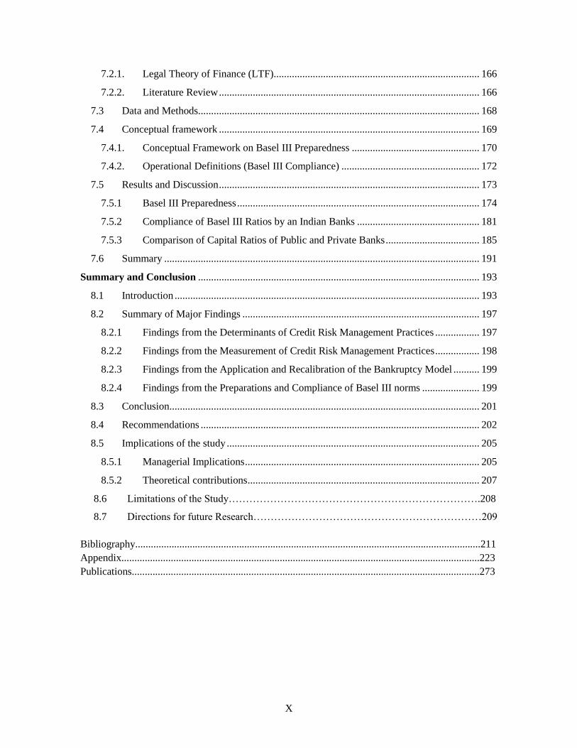
7.2.1. Legal Theory of Finance (LTF)............................................................................... 166
7.2.2. Literature Review .................................................................................................... 166
7.3 Data and Methods............................................................................................................ 168
7.4 Conceptual framework .................................................................................................... 169
7.4.1. Conceptual Framework on Basel III Preparedness ................................................. 170
7.4.2. Operational Definitions (Basel III Compliance) ..................................................... 172
7.5 Results and Discussion .................................................................................................... 173
7.5.1 Basel III Preparedness ............................................................................................. 174
7.5.2 Compliance of Basel III Ratios by an Indian Banks ............................................... 181
7.5.3 Comparison of Capital Ratios of Public and Private Banks .................................... 185
7.6 Summary ......................................................................................................................... 191
Summary and Conclusion ............................................................................................................ 193
8.1 Introduction ..................................................................................................................... 193
8.2 Summary of Major Findings ........................................................................................... 197
8.2.1 Findings from the Determinants of Credit Risk Management Practices ................. 197
8.2.2 Findings from the Measurement of Credit Risk Management Practices ................. 198
8.2.3 Findings from the Application and Recalibration of the Bankruptcy Model .......... 199
8.2.4 Findings from the Preparations and Compliance of Basel III norms ...................... 199
8.3 Conclusion ....................................................................................................................... 201
8.4 Recommendations ........................................................................................................... 202
8.5 Implications of the study ................................................................................................. 205
8.5.1 Managerial Implications .......................................................................................... 205
8.5.2 Theoretical contributions ......................................................................................... 207
8.6 Limitations of the Study……………………………………………………………….208
8.7 Directions for future Research…………………………………………………………209
Bibliography.....................................................................................................................................211
Appendix..........................................................................................................................................223
Publications......................................................................................................................................273
XI
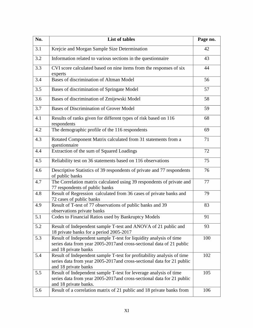
No. List of tables Page no.
3.1 Krejcie and Morgan Sample Size Determination 42
3.2 Information related to various sections in the questionnaire 43
3.3 CVI score calculated based on nine items from the responses of six
experts
44
3.4 Bases of discrimination of Altman Model 56
3.5 Bases of discrimination of Springate Model 57
3.6 Bases of discrimination of Zmijewski Model 58
3.7 Bases of Discrimination of Grover Model 59
4.1 Results of ranks given for different types of risk based on 116
respondents
68
4.2 The demographic profile of the 116 respondents 69
4.3 Rotated Component Matrix calculated from 31 statements from a
questionnaire
71
4.4 Extraction of the sum of Squared Loadings 72
4.5 Reliability test on 36 statements based on 116 observations 75
4.6 Descriptive Statistics of 39 respondents of private and 77 respondents
of public banks
76
4.7 The Correlation matrix calculated using 39 respondents of private and
77 respondents of public banks
77
4.8 Result of Regression calculated from 36 cases of private banks and
72 cases of public banks
79
4.9 Result of T-test of 77 observations of public banks and 39
observations private banks
83
5.1 Codes to Financial Ratios used by Bankruptcy Models 91
5.2 Result of Independent sample T-test and ANOVA of 21 public and
18 private banks for a period 2005-2017
93
5.3 Result of Independent sample T-test for liquidity analysis of time
series data from year 2005-2017and cross-sectional data of 21 public
and 18 private banks
100
5.4 Result of Independent sample T-test for profitability analysis of time
series data from year 2005-2017and cross-sectional data for 21 public
and 18 private banks
102
5.5 Result of Independent sample T-test for leverage analysis of time
series data from year 2005-2017and cross-sectional data for 21 public
and 18 private banks.
105
5.6 Result of a correlation matrix of 21 public and 18 private banks from 106

XII
2005-2017 taking into account 526 observations
6.1 Description of bankruptcy models 121
6.2 Results of the tested Altman Model on 21 public 18 private and 5
NWB
124
6.3 Altman Model Accuracy rate 125
6.4 Correlation Matrix of Recalibrated Altman Model 126
6.5 Coefficient Test of Recalibrated Altman Model 127
6.6 Results of Recalibrated Altman Model of 21 Public, 18 Private and 2
NWB
128
6.7 Recalibrated Altman Model Accuracy Rate 129
6.8 Result of Independent Sample T-test of Altman and Recalibrated
Altman Model
130
6.9 Bases of discrimination as per Robust Test 130
6.10 Results of tested Robust Test on 39 Indian banks 131
6.11 Comparison of Original and Recalibrated Altman Model with the
Robust test
132
6.12 Results of the applied Springate model on 21 public 18 private and 5
NWB
134
6.13 Model Accuracy Rate of Springate Model 135
6.14 Correlation Matrix of Recalibrated Springate Model 136
6.15 The Coefficient test of Recalibrated Springate Model 137
6.16 Results of Applied Recalibrated Model on 21 Public, 18 Private and 2
NWB
138
6.17 Model Accuracy Rate of Recalibrated Springate Model 139
6.18 Result of Independent Sample T-test of Springate and Recalibrated
Springate Model
140
6.19 Comparison of original and Recalibrated Springate Model with the
Robust test
140
6.20 Result of the tested Zmijewski model on 21 public, 18 private and 2
NWB
142
6.21 Model Accuracy rate of Zmijewski Model 144
6.22 Correlation Matrix of Zmijewski Model 145
6.23 Coefficient Test of Zmijewski Model 146
6.24 Result of the tested recalibrated Zmijewski model of 21 Public 18
Private and 2NWB
147
XIII
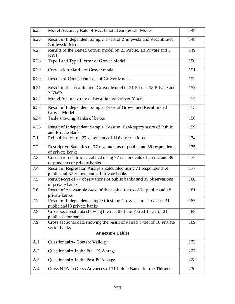
6.25 Model Accuracy Rate of Recalibrated Zmijewski Model 148
6.26 Result of Independent Sample T-test of Zmijewski and Recalibrated
Zmijewski Model
148
6.27 Results of the Tested Grover model on 21 Public, 18 Private and 5
NWB
149
6.28 Type I and Type II error of Grover Model 150
6.29 Correlation Matrix of Grover model 151
6.30 Results of Coefficient Test of Grover Model 152
6.31 Result of the recalibrated Grover Model of 21 Public, 18 Private and
2 NWB
153
6.32 Model Accuracy rate of Recalibrated Grover Model 154
6.33 Result of Independent Sample T-test of Grover and Recalibrated
Grover Model
155
6.34 Table showing Ranks of banks 156
6.35 Result of Independent Sample T-test in Bankruptcy score of Public
and Private Banks
159
7.1 Reliability test on 27 statements of 116 observations 174
7.2 Descriptive Statistics of 77 respondents of public and 39 respondents
of private banks
175
7.3 Correlation matrix calculated using 77 respondents of public and 39
respondents of private banks
177
7.4 Result of Regression Analysis calculated using 71 respondents of
public and 37 respondents of private banks
177
7.5 Result t-test of 77 observations of public banks and 39 observations
of private banks
180
7.6 Result of one-sample t-test of the capital ratios of 21 public and 18
private banks
181
7.7 Result of Independent sample t-testt on Cross-sectional data of 21
public and18 private banks
185
7.8 Cross-sectional data showing the result of the Paired T-test of 21
public sector banks
188
7.9 Cross sectional data showing the result of Paired T-test of 18 Private
sector banks
189
Annexure Tables
A.1 Questionnaire- Content Validity 223
A.2 Questionnaire in the Pre –PCA stage 227
A.3 Questionnaire in the Post PCA stage 228
A.4 Gross NPA to Gross Advances of 21 Public Banks for the Thirteen 230
XIV
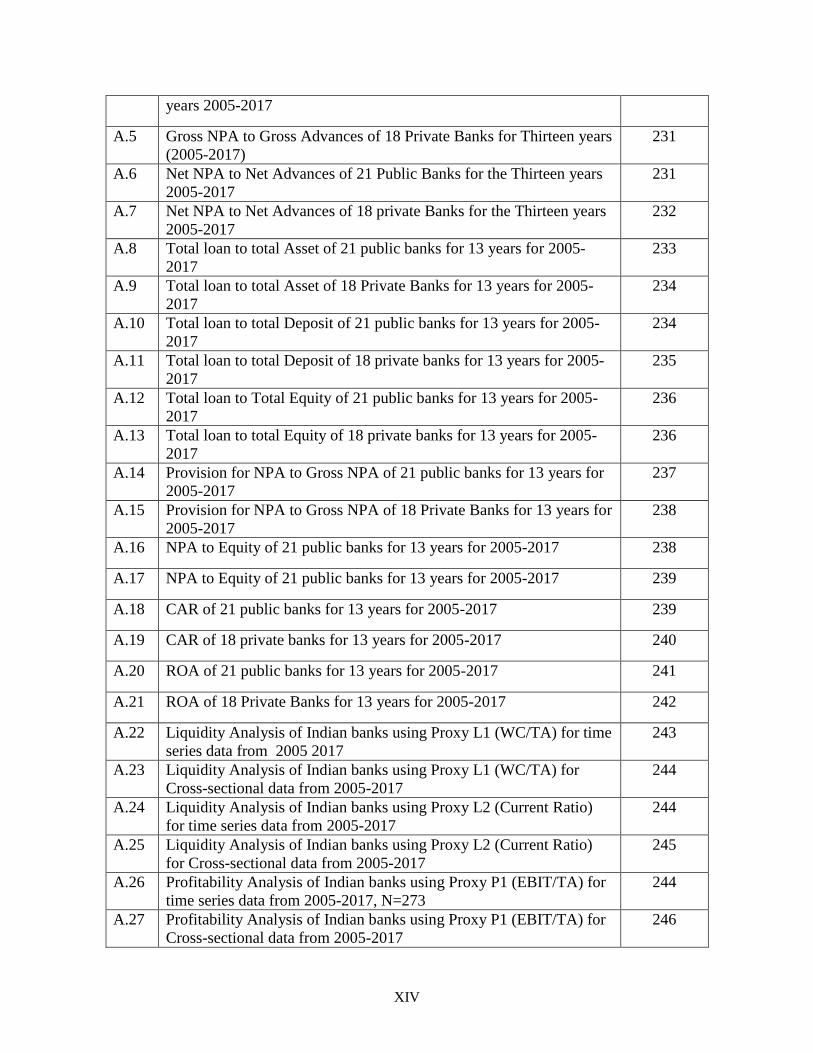
years 2005-2017
A.5 Gross NPA to Gross Advances of 18 Private Banks for Thirteen years
(2005-2017)
231
A.6 Net NPA to Net Advances of 21 Public Banks for the Thirteen years
2005-2017
231
A.7 Net NPA to Net Advances of 18 private Banks for the Thirteen years
2005-2017
232
A.8 Total loan to total Asset of 21 public banks for 13 years for 2005-
2017
233
A.9 Total loan to total Asset of 18 Private Banks for 13 years for 2005-
2017
234
A.10 Total loan to total Deposit of 21 public banks for 13 years for 2005-
2017
234
A.11 Total loan to total Deposit of 18 private banks for 13 years for 2005-
2017
235
A.12 Total loan to Total Equity of 21 public banks for 13 years for 2005-
2017
236
A.13 Total loan to total Equity of 18 private banks for 13 years for 2005-
2017
236
A.14 Provision for NPA to Gross NPA of 21 public banks for 13 years for
2005-2017
237
A.15 Provision for NPA to Gross NPA of 18 Private Banks for 13 years for
2005-2017
238
A.16 NPA to Equity of 21 public banks for 13 years for 2005-2017 238
A.17 NPA to Equity of 21 public banks for 13 years for 2005-2017 239
A.18 CAR of 21 public banks for 13 years for 2005-2017 239
A.19 CAR of 18 private banks for 13 years for 2005-2017 240
A.20 ROA of 21 public banks for 13 years for 2005-2017 241
A.21 ROA of 18 Private Banks for 13 years for 2005-2017 242
A.22 Liquidity Analysis of Indian banks using Proxy L1 (WC/TA) for time
series data from 2005 2017
243
A.23 Liquidity Analysis of Indian banks using Proxy L1 (WC/TA) for
Cross-sectional data from 2005-2017
244
A.24 Liquidity Analysis of Indian banks using Proxy L2 (Current Ratio)
for time series data from 2005-2017
244
A.25 Liquidity Analysis of Indian banks using Proxy L2 (Current Ratio)
for Cross-sectional data from 2005-2017
245
A.26 Profitability Analysis of Indian banks using Proxy P1 (EBIT/TA) for
time series data from 2005-2017, N=273
244
A.27 Profitability Analysis of Indian banks using Proxy P1 (EBIT/TA) for
Cross-sectional data from 2005-2017
246

XV
A.28 Profitability Analysis of Indian banks using Proxy P2 (ROA) for time
series data from 2005-2017, N=273
246
A.29 Profitability Analysis of Indian banks using Proxy P2 (ROA) for
Cross-sectional data from 2005-2017
247
A.30 Profitability Analysis of Indian banks using Proxy P3 (PBIT/CL) for
time series data from 2005-2017
248
A.31 Profitability Analysis of Indian banks using Proxy P3 (PBIT/CL) for
Cross-sectional data from 2005-2017
248
A.32 Profitability Analysis of Indian banks using Proxy P4 (TI/TA) for
time series data from 2005-2017
249
A.33 Profitability Analysis of Indian banks using Proxy P4 (TI/TA) for
Cross-sectional data from 2005-2017
249
A.34 Leverage Analysis of Indian banks using Proxy LV1 (RE/TA) for
time series data from 2005-2017
250
A.35 Leverage Analysis of Indian banks using Proxy LV1 (RE/TA) for
Cross-sectional data from 2005-2017
251
A.36 Leverage Analysis of Indian banks using Proxy LV2 (MVE/TL) for
time series data from 2005-2017,
251
A.37 Leverage Analysis of Indian banks using Proxy LV2 (MVE/TL) for
Cross-sectional data from 2005-2017
252
A.38 Leverage Analysis of Indian banks using Proxy LV3 (TD/TA) for
time series data from 2005-2017
253
A.39 Leverage Analysis of Indian banks using Proxy LV3 (TD/TA) for
Cross-sectional data from 2005-2017
253
A.40 Result of Altman Z-score of 21 public banks for 2005-2017 254
A.41 Result of Altman Z- score of 18 Private Banks for 2005-2017 255
A.42 Result of Altman Z-score of five NWB from 2005-2013 255
A.43 Result of Springate Model of 21 public banks for 2005-2017 255
A.44 Result of Springate Model of 18 private banks for 2005-2017 256
A.45 Result of Springate Model NWB banks from 2005-2014 257
A.46 Result of Zmijewski model for 21 public banks from 2005-2017 257
A.47 Result of Zmijewski model for18 Private banks from 2005-2017 258
A.48 Results of Zmijewski Model for NWB from 2005-2014 258
A.49 Result of Grover model of 21 Public Sector banks from 2005-2017 259
A.50 Result of Grover model for 18 Private Banks from 2005-2017 259
A.51 Result of Grover model for NWB banks from 2005-2014 260
A.52 Result of Recalibrated Altman Model of 21 Public and 18 Private
Banks
260

XVI
A.53 Result of Recalibrated Springate Model of 21 Public and 18 Private
Banks
261
A.54 Result of Recalibrated Zmijewski Model of 21 Public and 18 Private
Banks
262
A.55 Result of Recalibrated Grover Model of 21 Public and 18 Private
Banks
263
A.56 Questionnaire (Part 2): Preparedness in Basel III Implementation 264
A.57 Result of Tier I Capital Ratio from 2009-2018 267
A.58 Result of Tier II Capital Ratio from 2009-2018 268
A.59 Result of CAR from 2009-2018 269
A.60 Result of Leverage Ratio from 2009-2018 271

XVII
List of Abbreviations
AB Anticipated Benefit NPA Non-Performing Asset
AC Anticipated Cost NSFR Net Stable Funding Ratio
AI Anticipated Impact NWB Non - Working Banks
AR Availability of Resources OLS Ordinary Least Square
BP Basel III Preparedness PBIT/TA
Profit before Interest and Tax to
Total Asset (PBIT/TA)
CA/CL
Current assets / Current
Liabilities PBT/CL
Profit Before Tax to Current
Liabilities
CAR Capital Adequacy Ratio PCA Principal Component Analysis
CCB Capital Conservation Buffer RAA Risk Assessment Analysis
CCCB Counter Cyclical Capital Buffer RBI Reserve Bank of India
CRA Credit Risk Analysis RE/TA Retained Earnings to Total Asset
CRAA Credit Risk Assessment and
Analysis
RI Risk Identification
CRI Credit Risk Identification RMC Risk Monitoring Control
CRMC Credit Risk Monitoring Control RMP Risk Management Practices
CRMP Credit Risk Management
Practices ROA Return on Asset
CRU Credit Risk Understanding RWA Risk Weighted Assets
EBIT/CL
Earnings Before Interest and
Tax/Current Liability SEBI
Security Exchange Board of
India
EBIT/TA
Earnings Before Interest and Tax
to Total Asset TD/TA Total Deposit to Total Asset
EC Expected Challenge TI/TA Total Income / Total Asset,
FD Financial Distress TL Tolerance Level
LCR Liquidity Coverage Ratio TL/TA Total liabilities / Total Assets
LR Leverage Ratio URM Understanding Risk Management
MVE/TA
Market Value of Equity to Total
Asset VIF Variable Impact Factor
NI/TA Net Income / Total Assets WC/TA Working Capital to Total Asset
XVIII
ABSTRACT
Credit Risk is a significant threat for banks as the value of any organisation is measured by
its creditworthiness. Given the above, effective Credit Risk Management Practice (CRMP)
needs to be followed by banks to reduce this risk. The CRMP of public and private sector
banks in the Indian banking sector significantly differs as shown by past studies. In the
spirit of these studies, the present research assesses and compares the CRMP of the public
and the private banks in India, to check the extent and magnitude of variations. It is crucial
to study the lending and financial ratios of the banks as piling of NPAs adversely affects the
financial performance of the banks. Therefore the present study measures and compares the
credit risk management practices of public and private banks using lending ratio and
financial ratios.
Since ineffective CRMP may result in the bankruptcy of banks, the prediction of
bankruptcy by applying the bankruptcy model in the Indian banking context plays a
significant role. Due to some criticism of the models and the error rates that occurred in the
application of the model in present study, the current study aims at recalibration of the
applied models. Effective CRMP is possible due to precise control exercised by regulations
and supervision (Basel III norms). These controls pose challenges to bankers, which drives
the attention of bankers towards adequate preparedness needed for Basel III
implementation. Therefore the present study assesses the level of preparedness and
compliance of Basel III norms by public and private sector banks.
The present study used Principal Component Analysis (PCA) to determine the factors
influencing Credit Risk management Practices (CRMP) of banks. Descriptive statistics
were used to provide a summary of variables (CRMP determinants and Basel III
dimensions). In ratio analysis, lending and financial ratios were used to measure the credit
risk. Pearson’s Correlation Coefficient is used to find the relationship between financial
variables such as liquidity, profitability and leverage. An independent sample t-test is
conducted to compare the difference in credit risk determinants of CRMP, lending and

XIX
financial ratios, bankruptcy scores, Basel III preparedness and the Tier I, Tier II and CAR
between public and private banks in India. The test of ANOVA, along with a post hoc test
is conducted to find which bank reveals a statistically significant difference in the group.
One sample t-test and paired t-test was used on Basel III ratios. The robust test is conducted
to measure the financial health of the bank in the year 2017.
Regression Analysis such as, Ordinary Least Square (OLS) regression is used to determine
the statistical impact of the credit risk determinants on CRMP. Multiple linear regression is
used to measure the factors influencing the impact of the Basel III preparedness. Present
study applied Altman Z-score, Springate, Grover, and Zmijewski's model for assessing the
bankruptcy risk and also recalibrated these models by changing its coefficients through
multiple linear regression analysis.
In measuring the impact of the credit risk determinants on their respective CRMP for
public and private banks, regression results reveals that explanatory variable Credit Risk
Understanding and Credit Risk Assessment and Analysis (CRAA) among the four
components are most influential in the contribution of CRMP of private banks. The
regression model fits the data well for private banks compared to public banks in India. The
results of the Independent sample t-test show a significant difference in the credit risk
determinants between public and private banks.
In measuring the CRMP using lending ratios, it is observed that the certain lending ratios
are high in case of public banks. In measuring the CRMP using financial ratios, the result
states that both public and private banks experience low liquidity ratios and the leverage
ratios are lower for public banks and higher for private banks. The profitability ratios of
private banks show a fluctuating trend, and public banks show a decreasing trend.
The risk of bankruptcy of public and private banks was analysed by applying four
bankruptcy models. It is found that the results are not appropriate in case of two models.
The ranking results as per bankruptcy models shows that Bank of Baroda and Nainital Bank

XX
are in the first position (most efficient, and credit-risk safe) among public and private bank
respectively.
In measuring the statistical impact of factors of Basel III Preparedness, the regression
results shows that the factor ‘Anticipated Benefit’ is the most crucial followed by
‘Anticipated Impact’ in Basel III preparedness. The result of one-sample t-test shows that
private sector banks commenced disclosure towards compliance (minimum common equity
Tier I) ratio from 2018 while the public sector banks started compliance from 2014. The
private as well as public banks showed higher compliance of the Tier 1 capital ratio and
capital adequacy ratio, compared to a limit prescribed by Basel III norms.
Based on these findings, a broad conclusion can be drawn that private banks are generally
more efficient in terms of following credit risk management practices. The lending ratios
are low for private banks, indicating a better financial position. The bankruptcy study
concludes that the recalibrated Altman and the Grover model perform better than the
original model. In contrast, the original Springate and the Zmijewski model showed
improved accuracy over the recalibrated model. Further, it can be concluded that Indian
banks are well prepared to implement Basel III norms, as the Basel III ratios are maintained
by the public and private banks are at a much higher level than prescribed by RBI.
The study contributes to the literature in terms of the determination of credit risk
determinants of CRMP using the Principal Component Analysis (PCA) technique and
recalibration of bankruptcy models. The uniformity assumption of Institutional theory does
not apply in our study on account of differences in the understanding among employees on
the different aspects of credit risk and in the assessment and monitoring and control policies
of credit risk followed by the public and private banks in India. The private banks show a
negative relationship of factor, ‘Anticipated Cost’ with Basel III preparedness. These
results support the Legal Theory of Finance.

Chapter I Introduction
1
Chapter I
Introduction
1.1. Background of the Study
The health of a nation’s economy is largely dependent on a sound financial system. The
financial system provides necessary funds for the nation’s growth and development. In the
financial system, the banking sector occupies the most important position as it holds the
savings of the public provides a means of payment for goods and services and finances the
growth of business. The banks also play a major role in planning and implementing a
country’s financial policy (Itanisa 2016). Thus, a banking sector needs to be strong and
resilient for the strong economy of nation.
The word bank is derived from the French word banco or "bancus" or banc which means a
bench (Jhingan, 2001). The early Jews in Lombardy conducted the banking business by
sitting on benches. The banking is as old as the authentic history and the origins of modern
commercial banking are traceable in ancient times. According to Shekhar and Shekhar
(2008), in ancient Greece around 2000 B.C., the famous temple of Ephesus was used as
depositories for people’s surplus fund and these temples were the centres of money lending
transactions. The Priest of these temples acted as financial agent.
The period of banking reforms began in the year 1992, which provided a basis for looking
into the future of the Indian banking system (Kumar, 2014). During the last two decades,
there have been several reforms at the global and national levels that had an impact on the
operating environment of the banks. These reforms are in the form of, the introduction of
new players, new institutions, and new instruments. The introduction of new financial
products and services and the huge strides in technology and communication have brought
significant changes in the working of banks (Mallya 2012). These changes are gradual
liberalization of Indian banking, deregulation of interest rate, global competition, new
financial reforms, virtual banking, diversification of activities, retail character of banking,
liberalization of Foreign Direct Investment (FDI), active role of banks in upliftment of

Chapter I Introduction
2
socio-economic development of the country, implementation of new Basel requirement
etc. Given these above growing complexities in the bank’s business and the dynamic
operating environment, has led the banks to face a new or higher risk.
Risk is understood as “anything that can create hurdles in the way of achievement of certain
goals”. Therefore, the requirement of the risk management perceives a paramount
importance for the banks. According to Rao and Rentala (2012) the dynamic operating
environment of banks, have pushed the risk management to the forefront of the financial
landscape.
Risk management is understood as “adopting a practice of identifying the potential risk in
advance, analysing them and taking precautionary steps to reduce the risk”. Risk
management is significant because, today’s banks run its operation with two goals in mind
i.e. to generate profit and to stay in the business (Marision 2005), In other words, although
avoiding failure is the principal reason for managing risk but financial institution also have
broader objective of maximizing Risk Adjusted Rate of Return on Capital (RAROC).
According to Rao and Rentala (2012), the importance of risk management in banks is
because of their effect on the financial crisis and determining its role in the survival growth
and profitability of the bank. The risk management provides reasonable assurance of
achieving firm’s goals, compliance with applicable laws and regulations. It also helps in
encouragement of specific investment and decreasing the earnings volatility.
The risk management in banks witnessed a substantial change, due to emergence of
regulations evolved from the global financial crisis. As per these regulations the banks
need to retain higher standards for capital, leverage, liquidity, funding requirements and
risk reporting (Phillipe 2015). Although a variety of regulatory and supervisory authorities
have set norms for managing risk, still it remains a challenge for banks, as managing risk
depends on bank’s ability and stability. The process of risk management is complex and
difficult due to absence of risk culture in many banks. As the bank moved into a new high
powered world of financial operations and trading, with a new risk, there is a need for the
more sophisticated and versatile instrument for risk assessment, monitoring and controlling
risk exposure (Nandi and Chaudhary, 2011). The banks are expected to perform risk
management practice by designing effective risk management policies, designing a

Chapter I Introduction
3
procedure for identification and assessment of risk etc. Indian banking industry requires a
combination of new technologies, better processes of credit and risk appraisal, treasury
management, product diversification, internal control and external regulation for better risk
management (Adamson 2012).
Banks face three types of risk i.e. credit risk, market risk, and operational risk. Among
these risks, credit risk is the most important because it has a substantial effect on the return
on investment of the banks. According to Ngoroge and Ngahu (2017) Credit risk is a
significant threat for the banks as the value of any organization is measured by its
creditworthiness. Given the above, effective Credit Risk Management Practice (CRMP)
needs to be followed by banks to reduce this risk. The CRMP assumes establishing a
suitable credit risk management environment by identifying, measuring and managing
credit risk and covers all aspects such as identification of credit risk, understanding what
determines it and its measurement using various tools. The CRMP of public and private
sector banks in the Indian banking sector significantly differ as shown by the studies of
Thiagarajan (2011), Goel and Rekhi (2013), Kattel (2016) and Pourkeiki (2016). In the
spirit of these studies, the present research assesses and compares the CRMP of the public
and the private banks in India, to check the extent and magnitude of variations.
An ineffective CRMP may result in the bankruptcy of banks therefore, the prediction of
bankruptcy may help stakeholders to obscure themselves from the risks arising there from.
There are many models available for bank failure predictions. Literature survey shows that
the majority of international bank failure prediction employs the Altman-Z score model,
Grover model, Springate model and Zmijewski model. The present research aims to apply
all these models in the Indian banking context. Some critics of the above mentioned models
opine that when the original model is applied to a more recent sample, its predictive power
may be deficient and the risk of bankruptcy may be over predicted. Due to this fact, the
present study aims at the recalibration of the above models and compares the results from
the recalibrated and the original model, to judge its accuracy.
The effective CRMP is possible due to precise control by authorities in terms of regulations
and supervision. The concern regarding credit risk management at an international level

Chapter I Introduction
4
began in 1974, with the creation of the committee for regulation and supervision of banking
practices known as the Basel Committee on Banking Supervision (BCBS). Due to this
concern, the formal framework for bank’s capital structure was evolved in 1988 with an
introduction of Basel I. Basel I primarily focused on credit risk and appropriate Risk
Weighted Asset (RWA). The RBI implemented Basel I in the year 1992 in India. Basel I
was criticized for its rigidity of the "One Size Fit" approach and the absence of risk
sensitivity in capital requirements (Jayadev 2013). Due to these deficiencies in Basel I
accord, the BCBS introduced Basel II. Basel II is a much more comprehensive framework
of banking supervision when compared to Basel I (Sarma 2007). It was built on three
mutually reinforcing pillars such as Minimum Capital Requirements (Pillar1), Supervisory
Review (Pillar 2) and Market discipline (Pillar 3). Basel II was criticized for not
considering the liquidity and leverage risk in capital regulation and also failed to address
the systemic risk (Jayadev 2013). It was also criticized for its inability to prevent the
financial crisis; hence in response to the 2007-09 global financial crisis, BCBS issued Basel
III norms.
Basel III focused on four vital banking parameters viz. capital, leverage, funding, and
liquidity. Basel III introduced different aspects to control risk such as Counter Cyclical
Capital Buffers (CCCB), Capital Conservation Buffer (CCB), Leverage Ratio (LR),
Liquidity Coverage Ratio (LCR) and Net Stable Funding Ratio (NSFR). Basel III poses
several challenges to the bankers; risk managers, finance managers, and Basel III program
managers are under pressure to implement Basel III. The key challenges for these managers
will be deciding how best to implement a solution that allows them to comply with Basel
III (Whitepaper). These challenges drive the attention of bankers towards the adequate
preparedness needed for Basel III implementation. This prompts the present study to assess
the level of preparedness by public and private sector banks of Basel III norms.
India should transit to Basel III because of several reasons. By far the most important
reason is that, as India integrates with the rest of the world, as increasingly Indian banks go
abroad and foreign banks come on to our shores, we cannot afford to have a regulatory
deviation from global standards. Also, as per RBI guidelines, Basel III need to be

Chapter I Introduction
5
implemented in phases, due to this Basel III is not implemented fully by some of the banks.
This drives the attention of the researcher, to study the compliance of Basel III.
1.2. Statement of Problem
Over the current years, there has been an increased number of credit-related problems in the
banks due to increased Non-Performing Assets (NPAs). Moreover, the piling of NPAs of
public and private banks adversely affects the profitability, liquidity and leverage position
of banks. It is a worrying fact that public sector banks report higher NPAs than the private
banks. This NPA problem may be the result of ineffective CRMP. The result of ineffective
CRMP may lead to the breakdown of the whole banking system (Ishitiq 2015).
The other problem that guides this study is that recognising of exact determinants of CRMP
is difficult given the different factors that govern CRMP in different countries. The factors
applicable in some context/nations may not apply to Indian banks due to the difference in
the economic background and the Central Bank’s policies of the country.
The credit risk management is also a significant challenge for an Indian banking system due
to the constant heat of competition that banks face from foreign banks. This fact compels
the banks to look into its profitability, liquidity and leverage position, as the financial
position is positively affected by these three variables, or one is achieved at the cost of
others. Since the available literature state an inverse relationship between liquidity and
profitability and also between profitability and leverage, an effort is made to judge the
relation in the Indian context.
In today's era, the most common problems of the Indian banking sector are bank frauds and
hike in NPAs leading the banks towards state of bankruptcy. The stakeholders are
concerned about forecasting the likelihood of financial distress to respond before the event
takes place. Thus a variety of scoring models that can predict the bank failure have been
developed. Further, although the scoring model is one of the powerful tools used for
bankruptcy prediction, it also has its loopholes. Some authors question the model’s capacity
for sound default detection and argue that the bankruptcy prediction model is less accurate

Chapter I Introduction
6
when it is applied to a different environment, period and industry as compared to the reason
for which it was initially devised. The problem is that the prediction models used in this
research might have been for other industries rather than banking or may be outdated. Thus
the models may not provide credible results under all conditions and may need some kind
of calibration. This may lead to another problem. There may be a difference in the
predictive ability in the original and the recalibrated model, as a result both these models
may not match with each other due to change in coefficients. This demands a need for
comparing the results of both the models with the robust test, to decide the accuracy of the
models followed.
Furthermore, due to the above loopholes in the models, the reliability of the model is
doubtful; hence using a single model may not give a perfect result. Therefore, more than
one model needs to be used to predict bankruptcy. According to Kleinert (2014), single
bankruptcy prediction model faces limitations and use of multiple bankruptcy prediction
models improved the prediction accuracy.
The Basel III implementations need proper preparations as it involves huge cost and
resources in terms of capital, manpower and technology. Further, Basel III preparations are
affected by several factors i.e. Anticipated Benefit (AB), Anticipated Cost (Anticipated
Cost), Anticipated Impact (AI), Expected Challenge (EC), Availability of Resources (AR),
Education Level (EL) etc. Thus, there is a need to find the most significant factors
influencing its preparedness. The other research problem is related to compliance of Basel
III implementation by Indian banks. RBI has given the transitional schedule for
implementation of these new norms from the year 2013-2019. In this schedule, the
minimum requirement for Basel III ratios (CAR, Tier I, Tier II, leverage and liquidity ratio)
required to be followed by individual banks are prescribed by RBI. A reference to annual
reports show that some of the banks have recently moved towards Basel guidelines and are
still following standard approaches, but still many do not follow the expected advanced
approaches. This explains the need to study the compliance of Basel III norms in the Indian
context.

Chapter I Introduction
7
The other research problem is related to the pre and post-implementation phase of Basel III.
Capital ratios of the banks differ in the pre and post-implementation phase of Basel III.
Capital ratios of the banks need to be enhanced in the post-implementation of Basel III in
order to meet the higher requirements. Therefore the present study assesses Basel III ratios
in these two phases.
1.2.1 Research Questions
The research question underlying this study is recognizing the exact determinants of
CRMP. These determinants are not standard and as per the literature review it is observed
that, the factors governing the CRMP differs from country to country. In the past, some of
the studies undertaken in one country have used three determinants whereas some other
studies have used five determinants in other country. Thus, determinants applicable in other
context or country may not apply to the Indian banks. Therefore, the research question
addressing the above issue states, what are the determinants of Credit Risk Management
Practices in India? These different determinants have certain impact on the CRMP as per
the reviews of past studies. Therefore, a further question arises as, what is the impact of
these determinants on the CRMP?
The primary function of public and private banks is accepting deposits for lending. In
performing a lending function, both these banks undertake a heavy credit risk. Also, these
banks follow an equivalent procedure and safety precautions before sanctioning a loan and
are on equal foot of bearing the credit risk. Considering this fact, it is understood that there
is uniformity in the risk management practices among the public and private banks.
However it is a worrying fact that, public sector banks report higher NPAs than the private
banks. This triggers the researcher to find an answer to a research question such as, whether
there is a difference in the credit risk determinants of CRMP between public and private
banks?
Financial performance indicators such as, liquidity, profitability and leverage measured
through financial ratios helps public and private banks in knowing its financial position to
manage its credit risk. The financial position of both these banks may not be uniform as the
pattern and extent of liquidity, profitability and leverage differs between public and private
banks due to their nature of operations. Therefore, the research question arises, whether

Chapter I Introduction
8
there is significant difference in the financial ratios between the public and private banks?
The research gap from the literature review highlights the fact that the relationship between
liquidity profitability and leverage has been studied in other countries, but very few similar
studies have been carried out in the Indian banking sector. Therefore, the research question
arises to find - Whether there exists a particular trend and relations among liquidity,
profitability and leverage of Indian banks?
A study on lending ratio helps to understand the lending and NPA position of the banks.
As per the studies of Goel and Rekhi (2013) and kattel (2016) the credit risk management
practices of public and private banks differ. This difference in the CRMP may be on
account of various factors and one amongst them may be lending ratios. Due to this, a
question arises, whether there is a significant difference in the lending ratios between public
and private banks?
The bankruptcy models applied in the present study were originally developed at a different
time period, with different samples and were affected by the country’s economic
environment. Therefore the predictive power of these models may differ. Thus the question
arises as to how accurate are the bankruptcy models? If the predictive power of the model is
affected after its application to the Indian banking sector, the next question arises as to,
whether there is a need for the recalibration of these models to suit the current economic
environment and our specific regulatory environment of the country? After recalibration
and application of these models to the Indian banking sector, the study tries to answer the
question –Which financial distress model is accurate to predict bankruptcy of banks?
The financial position of the bank is assessed using bankruptcy score. Based on these
bankruptcy scores which Indian banks could be ranked as the best, and the worst? Lastly,
based on these scores, it further tries to answer a question whether there is significant
difference in the bankruptcy score of public and private banks?
It is crucial for the Indian banks to have good preparations for the Basel III implementation
in order to meet international standards. Therefore the question arises as to verify, whether
the Indian banks are prepared for the implementation of Basel III norms? The Basel III
preparations are affected by several factors as per the studies of Al- Tamimi (2008) and

Chapter I Introduction
9
Kapoor and Kaur (2015), with this raises the question as to, what are the significant factors
contributing towards Basel III preparedness? The Basel III preparations of public and
private banks may differ due to their nature of operation, availability of resources, etc.
Thus, further question arises whether there is statistical difference in the Basel III
preparations of public and private banks?
Basel III implementation poses a variety of challenges in terms of enhanced capital
requirements, design of comprehensive liquidity management framework, data acquisition
and software and hardware development. Therefore, some of the banks may not follow
these norms due to cost factor thus the question arises as to Whether Indian banks comply
with the minimum requirements of Basel norms stipulated by the RBI? The post
implementation period of Basel III requires banks to maintain higher capital to meet the
norms. Therefore, the question arises as to what is the difference in the Basel III ratios of
banks in the pre and post-implementation phase of Basel III? and whether banks have
followed required capital requirements in the pre and post-implementation phase of Basel
III?
1.3. Objectives of the Study
Following are the four objectives o this study:
1. To identify the factors (determinants) affecting the credit risk management
practices, measure its individual impact and compare them between public and
private banks.
2. To measure and compare the credit risk management practices of public and private
banks using lending ratios and financial ratios.
3. To analyse the risk of bankruptcy of public and private banks using the bankruptcy
models, judge their accuracy and rank the banks based on its score.
4. To assess the preparedness and compliance of the Basel III accord of public and
private banks in India.

Chapter I Introduction
10
1.4. Scope of the Study
The present study has been undertaken primarily to examine the CRMP of public and
private banks in India. Banks face three types of risk – Credit risk, Market Risk and
Operational risk. Among these risks credit risk is the most important one, because it has a
substantial effect on the return on investment of the bank. Therefore, present study is
restricted to credit risk, ignoring the other risk. There are different methods to measure
CRMP, however, the present study covers two methods i.e. credit risk measurement tools
and identifying determinants of credit risk.
The current study covers banks from two categories public sector banks and private banks.
There are 27 public sector banks in India, consisting of 19 Nationalised banks , six State
Bank group, Industrial Development Bank of India (IDBI) and Bhartiya Mahila Bank. The
present study covers 19 nationalized banks, State Bank of India and IDBI bank making it
twenty one public sector banks. There are 29 private banks (old and new private sector
banks) operating in the country, however the present study covers 18 private banks. The
type and the number of banks are selected based on the availability of data and the
consequences of time constraints.
Present study assesses the risk of bankruptcy of public and private banks using bankruptcy
models. There are many models available for bank failure predictions such as Standard and
Moody’s financial ratios, Beaver model, Altman Z- score model, Ohlson’s model CAMEL
model, Grover Model, Springate Model, Neural Network and Zmijewskis Model to predict
the health of the bank. Among these models, the present study focuses on the most
frequently used model in past studies. These models are the Altman-Z score model, Grover
model, Springate model, and Zmijewski model.
The accuracy of these models could be judged based on various factors; however present
study covers Type I and Type II errors, robust test and the ranks given to the individual
banks. The secondary data for the bankruptcy study is collected for thirteen years period
from the year 2004-5 to 2016-17. The data period consists of two phases, the pre-
implementation and the post-implementation phase of Basel II and Basel III norms. This is
the period where the Basel committee put norms on the banks and the effect of all these

Chapter I Introduction
11
norms is reflected in the financial statements of the banks, which are more reliable and will
reduce measurement errors.
Although a study concerning Basel III norms covers many aspects such as impact,
challenges, cost- benefit analysis etc, however, due to time and resource constraints present
study is limited to the assessment of the preparedness and compliance of Basel III norms
between select public and private banks in India.
A vast and intensive study is possible with respect to full compliance of these norms by the
Indian banking sector, but based on the data availability and time factor, present study,
focuses on compliance of Basel III ratios (Minimum Common Equity Tier I capital, Tier I
capital, Tier II capital, Capital Adequacy Ratio and leverage ratios). The other ratios such
as Liquidity ratio and Net Stable Funding ratio is not covered due to lack of data in the
annual statements.
1.5. Significance of the Study
The credit risk is a significant threat for banks as it has a direct impact on the profitability
of the bank. A study by Ishitiq (2015) found a positive relationship between the
performance and risk management. This relationship throws light on the paramount
rationale of management of credit risk. A study by Rehman (2016) states that credit risk
management is getting more attention, especially after the credit crunch of 2007-2009.
According to Ngoroge and Ngahu (2017) effective risk management can bring far reaching
benefits to all organisations, whether large or small, public or private sector. Therefore
efficient CRMP is one of the vital strategy bank needs to make by diverting its resources
for the growth and survival of banking business. This strategy of CRMP can give many
advantages to the financial institution in terms of financial performance, competitive
advantage, optimum utilisation of resources, improved service delivery, growth and
survival, reduced waste and developing policies for regulatory bodies.
The information about CRMP will assist in developing policies for regulatory bodies.
According to Onyano (2010) policy makers in the financial industry will use this study in
understanding the extent to which the banking industry is exposed to credit risks. This will

Chapter I Introduction
12
guide them in designing the best practices for the financial institution to manage credit risk.
The findings will further enhance the managers understanding of the key systems that will
improve the banks performance. Proper CRMP is also important because Ishitiq (2015)
found in its study that, there is positive relationship between the performance and risk
management. In addition to the regulatory requirement, the CRMP is valuable and relevant
in order to increase the value of the firm (Ishitiq 2015).The value of financial institution is
judged based on its financial performance. The credit risk management is found to be one
of the determinants of returns of banks stock (Hussain and Ajmi, 2012). Thus the credit risk
management will maximize the banks risk adjusted rate of return by adjusting credit risk
exposure within acceptable limit.
It is crucial to study the lending and financial ratios of the banks as piling NPAs adversely
affects the financial performance of the banks. A study on measurement of credit risk using
lending and financial ratios is significant to managers, investors, creditors, government and
regulators. Managers can depend on these ratios to have the right choice in the decision-
making process and efficiently adopt new policies and a new management system. These
ratios help the investors to predict the future situation, earning capacity of their invested
companies and the safety of their investments. The ratio analysis assist the creditors in
knowing the ability of a company to pay off its debt and the company's potential in the
future to keep lending it. The ratios aid government to compare individual bank with the
industry ratio to provide financial support for the weaker banks and could help the bank
regulators to evaluate and compare banks performance.
The bank health needs attention because banking is a business entity that collects funds
from the public in the form of savings and Chanel’s to the community in the form of credit.
This process attaches the risk that the borrower may default on his application. This
uncertain economic environment during recent years has stressed the importance
bankruptcy prediction. In such a condition it becomes necessary to assess the financial state
of the banks using distress prediction model to estimate the business risk. This study will
help the banks to understand its financial position much in advance and to avoid financial
distress.
Chapter I Introduction
13
A proper prediction of bank bankruptcies is significant as the financial sector is very crucial
for a growing economy, and any variations in its performance can affect the economy either
way (Chaudhary and Nandi, 2011). The bankruptcy information is useful to the
management to undertake precautions and essential to the auditor to report on the viability
of the firm. Investors are interested in the bankruptcy model to avoid the risk of loss from
an unsuccessful investment, and the lenders are interested in taking decisions on the
granting of loans to the bank. The government agency has an interest in seeing the signs of
bankruptcy to provide support for its revival. Score value calculated using models is useful
to banks to demand loans from RBI or any other funding agency as per Pradhan (2014).
Thus the financial health of banks can help each beneficiary and it can be applied in a wide
variety of situations. Bankruptcy study will provide information on variables that will
influence the health of a bank (Stingar and Warstuti 2014). In total, if bankruptcy could be
predicted with reasonable accuracy ahead of time banks could better protect their business
and could take action to minimize risk and loss of business perhaps even prevent
bankruptcy (Ramage and Pongstal 2004).
The progress report on the implementation of Basel III regulatory framework (2013)
reflects that RBI has taken the steps for convergence of the International Basel standards
and the Indian banks need to transit to Basel III because of several reasons. The most
important reason being, the Indian banks make it presence in the world and foreign banks
come on to our shores. Hence the Indian banks cannot afford to have a regulatory deviation
from global standards. Considering this fact, preparedness of Indian banks for the
implementation of Basel III norms assumes a high level of significance. Further, it is also
significant because it poses a variety of challenges to the banks. These challenges drive
them to develop technological infrastructure and human resources to cope up with risk
environment.
A major challenge for the Indian banks is the implementation of regulations as per the
transitional schedule specified by RBI. In the post-implementation period of Basel III
norms, the banks need to infuse an additional capital, to maintain quantity, quality,
consistency, and transparency of capital as per set norms. According to Athira and Shanti
(2014), banks require additional capital of 5 lakh crores and further the public sector banks

Chapter I Introduction
14
require common equity of 1.4 - 1.5 trillion to meet Basel III requirements. Apart from this,
Basel III norms require banks to follow the Capital Conservation Buffer and Counter
Cyclical Capital Buffer for the better risk management framework. All these stipulations
trigger the banks to enhance their capital base by balancing the profitability aspects of
banks. These facts trigger the significance of Basel III preparations.
Due to the above challenges, RBI introduced phase in arrangement for the implementation
of Basel III norms from 2013-14 to 2018-19, which will also align full implementation of
Basel III in India closer to the internationally agreed date of January 1, 2019. Thus, all
banks are proceeding at their own pace for meeting the Basel III requirements. Therefore, a
study on the compliance of Basel III norms as per the transitional schedule specified by
RBI perceives paramount importance.
The evolution of Basel III norms has taken place due to the impact of the financial crisis in
2008. This crisis affected the U.S. economy and other economies very badly as the capital
was dried up during this crisis. However, the impact of the same was less on the Indian
economy, maybe due to the better capital position of the Indian banks in this period. This
period was known as the pre-implementation period of the Basel III norms and in this
period the capital position of the Indian banks was sufficient to face the financial crisis. The
post-implementation period of Basel III norms shows an improvement in the minimum core
capital stipulations. Thus there is difference in the capital ratios in the pre and post-
implementation period of Basel III norms. Therefore, a comparative study on the Basel III
capital ratios of the public and private banks in the pre-implementation phase and also in
the post-implementation phase achieves due importance.
The present study is also significant as it makes valuable contribution to the current
academic literature in the area of banking and also proposes methodologies as well as
practical additions to the key area. Furthermore, it will act as a source of reference and
background for other research in this area plus findings will stimulate the future research.

Chapter I Introduction
15
1.6. Organisation of the Study
Our study titled “A Study of Credit Risk Management Practices of Public and Private
Banks in India” is organized into eight chapters, and is arranged as follows:
Chapter I: Introduction: This chapter throws light on the background of the study,
statement of the problem, research questions, objectives of the study, scope of the study,
significance of the study, and organization of the study.
Chapter II: Theoretical Foundations and Empirical Literature: This chapter explores
exhaustive and comprehensive literature on Credit Risk management Practices (CRMP),
bankruptcy models and compliance and preparedness of Basel III norms. The review of
literature allows understanding the gaps in prior studies.
Chapter III: Methodology and Techniques: This chapter begins with specifying details
of data sources such as the primary data and secondary data. Further, it covers in detail
hypotheses of the study and the statistical tools used for data description, data validity, and
data analysis. It also covers elaborations on the recalibration of bankruptcy models and
robust tests.
Chapter IV: Determinants of CRMP: This chapter covers the identification of the credit
risk determinants of CRMP, measurement of the impact of these determinants on CRMP,
and the comparison of these determinants between public and private banks in India.
Chapter V: Measurement of CRMP: This chapter measures the CRMP using lending
ratios and financial ratios. Further, it also finds the relationship between liquidity,
profitability and leverage variables.
Chapter VI: Application and Recalibration of Bankruptcy Model: This chapter applies
the Altman Z-score, Springate, Grover, and Zmijewski's, model for assessing the
bankruptcy risk of select public and private banks in India. It also recalibrates these models

Chapter I Introduction
16
and further judges the accuracy of the models and compares the bankruptcy scores of public
and private banks.
Chapter VII Preparedness and Compliance of Basel III Norms: This chapter assesses
the preparedness and compliance of Basel III accord in the Indian banking industry. It
measures the impact of factors of Basel III preparedness on the relevant variables. The
compliance part covers the comparison of actual Basel III ratio of banks with minimum
ratio specified by the RBI. Additionally, it presents the comparison of the Basel III ratios
between public and private banks in the pre-implementation phase and also in the post-
implementation phase of Basel III. Further, it covers the comparison of these ratios before
and after the adoption of Basel III norms.
Chapter VIII Summary and Conclusion: In the concluding chapter, the results and
findings are summarised based on each chapter. Further, it also covers the
recommendations to the stakeholders, contributions of the study in terms of managerial and
theoretical, and finally, it includes directions for future research.

Chapter II Theoretical Foundations and Empirical Literature
17
Chapter II
Theoretical Foundations and Empirical Literature
2.1 Introduction
In 1980s literature put heavy emphasis on a conceptual study of banks and their functions.
In the year 1992 Narsimah committee introduced banking reforms and various measures
were put forth on the banks in the form of capital adequacy norms, phase out of Non-
performing Assets (NPA) etc. This has triggered the researchers and financial writers to
develop a literature on the compliance of banking reforms. Over a period of time, other
regulations came into force such as prudential norms and Basel norms which also made
ample contributions in the banking literature. The reason for the evolution of these norms is
due to inadequate CRMP followed by the banks leading them on the path of bankruptcy.
Thus present study covers CRMP, bankruptcy models and banking regulations such as
Basel III norms. Although, most of the banking literature acknowledges risk management,
bankruptcy models and Basel norms, there has been relatively little research undertaken on
comparison of CRMP between public and private banks in India, assessment of the
financial health of the banks using bankruptcy models, and preparedness and compliance of
Basel III norms.
The review of studies concerning CRMP is helped to understand the credit risk
determinants affecting CRMP and the tools used by banks to measure credit risk. The
literature on bankruptcy predictions is needed to understand the conceptual clarity and
working of bankruptcy models. Similarly, reviews on Basel III norms are required to
understand the mechanism used in other studies for Basel III preparedness and Compliance.
The objective of this chapter is to explore the available literature on CRMP, bankruptcy
models and preparedness and compliance of Basel III norms. This chapter is divided into
three parts. Part I discusses some important theories and descriptions on bankruptcy
models. Part II reviews the studies on credit risk determinants and measurement of CRMP,
bankruptcy models, preparedness and compliance of Basel III norms. Part III focuses on the
research gap and summarises the whole chapter.

Chapter II Theoretical Foundations and Empirical Literature
18
2.2 Theoretical Framework
The study relies on the theories that may have underpinnings to the issue of CRMP and
Basel III preparedness. It further comprises a brief description of bankruptcy models such
as the Altman Z-score model, Springate model, Zmijewski model, and Grover model.
2.2.1 Theory Relating to CRMP and Basel III Preparedness
The researcher resolved the controversy on understanding the difference in the credit risk
determinants of CRMP between public and private banks, with the aid of Institutional
Theory. The other issue relating to understanding the significant contributor to the Basel
III norms preparedness was resolved with the help of Legal Theory of Finance.
2.2.1.1 Institutional Theory
The Institutional Theory (the IT) is based on understanding the theoretical framework in
context to the organizational phenomena. The IT considers the process by which structures,
schemes, rules, norms, and routines become established as authoritative guidelines for
social behaviour as per Scott (2014). This theory describes norms, ideologies, values, to be
uniformly followed by all, to run their organizations. The studies by Collier and Woods
(2011) and Hudin and Hamid (2014) used this theory in describing the concept of risk
management implementation. Their studies put forward that institutionalization exists when
the risk management activities in most of the institutions become highly equivalent. This
equality can be gained through the coercive isomorphic method by which political and
regulatory pressures are employed in the institutions.
It can deduced from this theory that regulatory pressures, enduring practices and structures
will set uniform conditions of actions, triggering highly homogeneous risk management
practices in banks. Thus according to the IT, there is some homogeneity expected with
respect to CRMP of different type of banks operating within the same environment. In
simpler terms uniform regulatory pressures, norms, and expected compliance requirements
bring uniformity in the CRMP of all the banks.

Chapter II Theoretical Foundations and Empirical Literature
19
2.2.1.2 Legal Theory of Finance (LTF)
Legal Theory of Finance was proposed by Pistor (2013) and considered as a cornerstone for
the political economy of finance. The author argues that finance is hierarchical and the
stringent enforcement of legal obligation in the financial market which depends on one’s
hierarchy in the financial network. The theory is based on the assumption of fundamental
uncertainty. This assumption upholds the fact that, during the time of financial crisis,
stringent enforcement of legal obligations would lead to the self-destruction of the financial
system. Therefore, this theory states that the cut down of execution of the law is necessary
for the survival of the financial system. The author claims that, in the past, it is observed
that, although the law tends to give credibility through its enforceability, the actual
implementation of legal commitment without making changes in it had brought down the
financial system. LTF is an inductive theory, which argues that, there is an inverse
relationship between the obligatory nature of contractual and legal commitments on one
hand and the hierarchical nature of finance on the other, where law tends to be more elastic
at the apex and binding on the periphery of the financial system (Pistor, 2013). The
elasticity of law states that law is not equally binding throughout the system.
It is observed from the theory that if the stringent implementation of laws puts the financial
institution in a dire situation of survival, then the suspension of the full force of law is a
priority for the survival of the financial institution. This theory could be related to
understanding the contributory factors for the Basel III preparedness by the banks. In case
the cost incurred for the enforcement of norms exceeds the benefits derived, then it will be
prudent not to implement these norms for the survival of the banks.
2.2.2 Bankruptcy Models
Present study used scoring model such as Altman Z-score model, Springate model,
Zmweskis model and Grover model to predict bankruptcy of banks.

Chapter II Theoretical Foundations and Empirical Literature
20
2.2.2.1 Altman Z-Score Model -1968
Edward Altman, Finance Professor at Stern School of Business of New York University
developed this model to predict the likelihood of bankruptcy of a manufacturing company.
He believes that the univariate prediction model served in most cases as an indicator and
not as a predictor of bankruptcy. Before the development of the model, he used 22 tentative
variables as a significant predictor of bankruptcy from the five areas such as liquidity,
profitability, leverage, solvency, and activity. He ran multiple discriminant analysis
repeatedly with different mergers of these ratios according to individual contributions,
inter-correlations, and the forecasting ability of each merger. Finally, he developed a Z-
Score model based on five variables that had the most predictive power in the multivariate
discriminant analysis model and gained the accuracy rate of 94%. In his model, he used 33
bankrupt and 33 on- bankrupt firms covering a period of 1946-1965. His model gains an
accuracy rate of 94%. His model was the most influential in corporate bankruptcy
prediction as it was a multivariate model build on the values of selected ratios.
Later this model was re-estimated for service companies in the year 1993 and made use by
many researchers in the past such as Shumway (2001), Altman (2000), Chaudhary and
Nandi (2011), Popker (2013), Chieng (2013), Sharma and Mayanka (2013), Chotalia
(2014), Pradhan (2014), Cantemir and Cristana (2014) Lin (2015), Maina and Sawka
(2017) and Khaddafi et al. (2017).
2.2.2.2 Springate Model -1978
The Springate model was the first model to be introduced by Gordon LV Springate and
used for 40 companies using four variables to determine its scores. This model is a
revolution of the Altman model and it is a strong alternative to Altman’s research as per
Cantemir (2014). In development of model, he initially used 19 financial ratios that have
been frequently used. However, after testing the model, he finally chose four financial
ratios to develop a final model. Springate model examines insufficient liquidity, excess
debt, insufficient sales and lack of profit as the factors to determine the health of firms.
Springate used 40 companies as the sample for his research and shows an accuracy rate of
92.5 percent. A study by Arasu (2013), reports that the Springate model was tested using

Chapter II Theoretical Foundations and Empirical Literature
21
forty companies and achieved a bankruptcy prediction rate of 92.5%. The Springate model
was applied in the literature by Sajjan (2016), Husein and Pambekti (2014), Imanzadeh et
al. (2011) and Timmermans (2014).
2.2.2.3 Zmijewskis Model -1984
Finance scholar Mark E. Zmijewski created a financial distress prediction model based on
Ohlson’s (1980) work, and now is popularly known as the ‘Zmijewski model’. Zmijewski
used the probit method to predict bankruptcy by considering external factors such as
industry sector, size of the firm, economic cycle in which it operates etc. Zmijewski model
was not a pioneer in applying probit analysis in bankruptcy prediction; however he is the
first who developed a general probit model. Zmijewski argues that one need to builds a
model based on the entire population, to avoid the bias in estimated coefficients; hence he
tried to avoid the choice-based sample bias in his model. He observed that most of the early
models of predicting bankruptcy suffered from this bias. The sample used was non-
financial, non-service and non-public administration firms listed on the American and New
York stock exchange from 1972-78 comprising of 40 bankrupt and 800 non-bankrupts
firms. The original model reported an accuracy rate of 98.2 percent and was later used by
Mehrani et al. (2005), Imanzadeh et al. (2011), Timmermans (2014), Husein and Pambekti
(2014) Warstuti and Stinjak (2014), and Monousaridis (2017).
2.2.2.4 Grover’s Model - 2003
The ‘Grovers Model’ is developed by the restoration of the Altman Z model by Jeffrey S.
Grover by using a sample of 70, comprising of 35 bankrupt and 35 non-bankrupt firms. The
data period was from 1982 to 1996. During the development and testing of the model he
used the sample according to Altman Z-score and he took working capital to total asset and
EBIT to total asset variable of the Altman model and then adds profitability ratios which
are indicated by ROA. According to Prihanthini and Sari (2013) this model had a very high
accuracy rate compared to the Springate model, Zmijewski's model and Altman Z-Score to
measure bankruptcy in a food and beverage company listed in the Indonesian stock
exchange. This model has been applied by Prihanthini and Sari (2013), Aminian et al.
(2016), Qamruzzaman (2016) and Primasari (2017).

Chapter II Theoretical Foundations and Empirical Literature
22
2.3. Empirical Literature
Past studies undertaken in India and abroad on the credit risk determinants and
measurement of CRMP, bankruptcy models and preparedness and compliance of Basel III
norms have been reviewed extensively by the researcher.
2.3.1. Literature on the Determinants of CRMP
The primary objective of the present study is to identify the factors (determinants) affecting
credit risk management practices, measure its individual impact and compare them between
public and private banks. To achieve this objective present study covers the literature on the
determinants affecting CRMP. In the beginning, studies relating to the conceptual
framework of risk and risk management practices were reviewed. Studies by Benar (2001),
Rosman (2009), Purukaystha and Raul (2014), Harie et al. (2015), and Aven (2016) provide
a historical perspective and conceptual framework of risk and risk management practices.
Their studies point out the phenomenal changes that have taken place in risk management
practices of the Indian banking sector and also explain the relationship between risk
management practice and risk management process.
A study by Diksha and Arora (2009), Bharadwaj (2013) and Subramanyam et al. (2016),
throws light on the weakness of the corporate governance structure of the banks, leading to
improper management of credit risk by banks. Bharadwaj (2013) made an empirical study
on awareness and practices of credit risk management by two banks from Ludhiana city
with a sample of 60 respondents. The data was analyzed data using descriptive statistics,
Chi-square and t-test and concludes that majority of respondents are unaware of the credit
risk management framework. Diksha and Arora (2009) critically examined the risk
management practices of three banks using primary and secondary data. The research
concludes that most of the banks do not have a risk management team, policy, procedure,
and appropriate corporate governance structure in place. Subramanyam et al. (2016)
selected seven Indian banks to study whether the concept of risk management features in

Chapter II Theoretical Foundations and Empirical Literature
23
corporate meetings, and concludes that risk management is rarely discussed in the
meetings.
According to Nazir et al. (2012) efficient risk management practices are in need today,
because these practices will not only increase the return but improve the competitive
strength of banks. However, less efficient Risk Management Practices (RMP) could make
the situation of the bank worse. Empirical literature is available on conceptual studies of
Risk Management Practices and the factors affecting the RMP (Rosman, 2009). A study by
Das (2005), conducted a conceptual study on determinants of RMP, and presented
guidelines on various determinants of RMP. A similar study was conducted by Rosman
(2009) on Islamic banks, and stated the use of four determinants to develop risk
management model and also suggest a positive relationship between the determinants of
risk management and RMP.
A conceptual study put in practice and empirically proved has wider acceptance. Several
researchers conducted an analytical study on finding out the relationship between the RMP
and its determinants. Studies by Al-Tamimi and Al- Mazrooei (2007), Ochola (2010),
Shafiq and Nasr (2010), Nazir et al. (2012), Hussiney (2012), Gakure et.al (2012), Hussain
and Al-Ajmi (2012) and Ishtiaq (2015) have applied RMP models on different banks in
their countries.
A study by Al-Tamimi and Al-Mazoorie (2007), examined the five determinants of Risk
management Practices (RMP) of UAE national and foreign banks with the aid of Ordinary
Least Square (OLS) regression. The results indicate that there is a significant difference
between the UAE national and foreign banks in two determinants of RMP. A study by
Ochola (2010) analyzed primary data on the five determinants of credit risk management
practices used by commercial banks in Kenya with the help of descriptive statistics. Its
study concluded that one factor, i.e. credit risk monitoring score is low, indicating the
inefficiency of banks in monitoring credit risk. A study by Shafiq and Nasr (2010) explored
and compared the five determinants of RMP followed by public sector commercial banks
and local private banks in Pakistan with the aid of OLS regression. The result revealed a
significant difference in the application of determinants of RMP among public banks and
local private banks. A study by Nazir et al. (2012) compared the RMP of conventional and

Chapter II Theoretical Foundations and Empirical Literature
24
Islamic banks in Pakistan using five determinants with the help of regression. The result
indicated that there is a significant difference in the determinants of RMP of Islamic and
conventional banks. A study by Gakure et al. (2012) investigated the effect of the four
determinants of credit risk management practice on the performance of unsecured bank
loans of commercial banks in Kenya and the result indicated a positive effect of two
determinants on the performance of banks. A study by Hussain and Al-Ajmi (2012)
examined the association of the determinants of RMP with the conventional and Islamic
banks using different econometrics and statistical method. This study used five factors to
judge its impact on the RMP using the OLS technique. The study found that the level of
risk is significantly higher in conventional banks. A study by Ishitiaq (2015) assessed the
potency of eight determinants of risk management within banks in Pakistan with the help of
OLS regression. Its study concluded that effective RMP depends upon several determinants
and is useful exercise to meet regulatory requirements. A study by Ngoroge and Ngahu
(2017) used one factor, i.e. Risk Identification (RI) to find its impact on the performance of
the banks in Kenya. Its study concludes that risk identification played a crucial role in the
credit performance of the banks. Hussiney (2012) examined the different techniques of
RMP dealt with within banks in UAE. The result indicated a narrow range of risk and
unuses of diverse range of RMP in the UAE banks.
2.3.2. Literature on Measurement of CRMP
Another aim of the present study is to measure the CRMP of public and private banks
through lending and financial ratios as credit risk measurement tools. It is found from the
literature that, the ratios for measurement of credit risk differs from bank to bank although
all the banks face the same type and extent of credit risk. A studies by Thiagarajan (2011),
Goel and Rekhi (2013), Kattel (2016), and Pourkiaei and Kumar (2016) investigated the
difference in the credit risk of public and private banks using different ratios for
measurement of credit risk.
A study by Thiagarajan (2011) measured and compared the credit risk between public and
private banks using tool such as ratio analysis and ANOVA test. The result shows a
significant difference in the ratios of public and private banks. Similarly, a study by

Chapter II Theoretical Foundations and Empirical Literature
25
Pourkeiki (2016) measured and compared credit risk between public, private and foreign
banks using a tool i.e. ratio analysis and T-test. The result shows a significant difference in
the ratios of public, private and foreign. A study by Kattel (2016), found a significant
difference in credit risk of private and joint-venture banks in Nepal using a tool i.e. one way
ANOVA. A study by Goel and Rekhi (2013) compared the performance of public and
private banks based on indicators such as profitability and capital ratios with the help of
descriptive statistics. This study concludes that new banks are more efficient than old ones.
The present study also covers the measurement of CRMP using liquidity, profitability and
leverage variable, with the assistance of financial ratios. The liquidity, profitability and
leverage are found to be the essential determinants for the success and survival of the
banks; hence there should be optimum tradeoff between these three variables. Considering
the above present study finds the interrelationship between these three variables and
measures CRMP using these variables.
Past studies were reviewed, to understand the interrelationship between these three
variables. It is identified from the reviews that, in certain banks there is positive
relationship between liquidity and profitability, whereas other banks showed no
relationship between these two variables. This shows that, there persists a controversial
issue on the relationship of these two variables. There are studies such as Lartey et al.
(2013), Awais et al. (2016), Nabeel and Hussain (2017), which shows a negative
relationship between liquidity and profitability in banking industry.
A study by Lartey et al. (2013), found a weak relationship between liquidity and
profitability of the banks listed on the Ghana stock exchange. Similarly, Awais (2016)
developed a relationship between profitability and liquidity using the regression model. The
empirical results reveal that there is a significant negative relationship between banks
liquidity measurement and ROA ratio. Also, Nabeel and Hussain (2017) examined the
effect of liquidity management on profitability in the banking sector of Pakistan. Data were
analyzed using correlation and regression techniques. Its study concludes that cash and
current ratios show negative relations whereas quick and CAR show positive relations
towards profitability.

Chapter II Theoretical Foundations and Empirical Literature
26
The studies which show no relationship between liquidity and profitability are Abdullah
(2014) and Ahmed (2016). A study by Abdullah (2014) analysed the impact of liquidity on
profitability in the banking sector of Bangladesh and concluded that there is no significant
relationship between liquidity and profitability. Also a study by Ahmed (2016) does not
show a significant relationship between profitability and liquidity. Its study was conducted
in Pakistan on standard chartered bank. Finally there should be an optimum tradeoff
between profitability and liquidity for the survival of the bank.
A leverage ratio measures the extent to which a bank has financial assets with equity. The
leverage ratio places a cap on the borrowings as a multiple of banks equity. Empirical
literature is available, stating the relationship between profitability and leverage. Most
studies found an inverse relationship between profitability and leverage. These studies are
Ebiringa (2012) Taani (2013) and Zafar and Fartyal (2015).
A study by Ebiringa (2012), analyzed the effect of financial leverage on Nigerian bank
performance, the study found a negative effect of leverage on the performance of the bank.
Research by Taani (2013) examined the impact of leverage on the profitability of Jordan
banks. Its study concludes that the presence of high leverage affects the return on banks. A
study by Zafar and Fartyal (2015) analyzed the leverage position of the Indian banking
industry and its impact on the profitability for a period 2001-2010. Its study concludes that
leverage has an impact on the profitability of the banks. High leverage may reduce the
profitability of the firm hence banks should make efforts to control the risk. Thus most of
the studies claim a negative relationship between leverage and profitability. However a
study by Moghaddam (2017) covered the effect of leverage and liquidity ratios on the
earnings of banks listed on the Tehran stock exchange for a period of 2010-2015 using a
multivariate regression model. The study concludes that there is a significant positive effect
of liquidity and leverage on the earnings of the firm.
A literature in the area of understanding relationship between liquidity and leverage is less,
as also the liquidity and its effect on the debt level have been a controversial issue among
scholars in finance studies. Prior studies have demonstrated that liquidity increased debt
level while other studies found that high liquidity was less leveraged and more regularly

Chapter II Theoretical Foundations and Empirical Literature
27
financed by their capital. A study by Ghasemi and Rajak (2016) concludes that a quick ratio
has a positive effect on leverage, whereas the current ratio harms the leverage of banks.
There is a difference in the profitability, liquidity and leverage position of public and
private banks in India. Most of the studies claim that there is a difference in these variables
of public and private banks. The work by Thakarshibai (2014), Balaji and Kumar (2016),
Patel and Bhanushali (2017),Vadrale and Katti (2018), Khan (2018) and Koley (2018)
conclude that the profitability position of a private bank is better than public banks.
A study by Thakarshibai (2014), analyzed the relative profitability of public and private
banks using ANOVA and descriptive statistics. Its study concludes an improvement in the
profitability of private banks compared to public banks. A study by Balaji and Kumar
(2016) compared the financial position of selected public and private banks in India using
profitability ratios. Its study concludes that the profitability is higher for the private banks
and the public banks are lacking behind in many financial parameters and are undergoing
many challenges too. Chintala (2016) compared the financial performance between public
and private banks in India. Its study found profitability is higher for private banks. A study
by Patel and Bhanushali (2017) made a comparison of nationalized and private banks for a
data period of 2010-2015 on profitability aspects. Its study concludes that both these
sectors are profitable but it is a greatest challenge for public banks. Also, Katti and Vadrale
(2018) compared the profitability position of public and private banks in India for a period
of 2001 to 2015. Their study concludes that the profitability position of the private bank is
better than public banks. A study by Khan (2018) analyzed the financial performance of
public and private banks through the CAMEL model and made a comparison through t-test.
Its study concludes that the performance of the private bank is better in all aspects
compared to public banks. Further, a study by Koley (2019) compared the performance of
public and private banks using the CAMEL model. Its study concludes that private banks'
performance is better than public sector banks. Similarly, Sharma (2017), made a
comparison and analysis of the profitability of private banks using ANOVA. The result
shows a difference in the profitability of banks in two financial ratios out of the four ratios
used in the study.

Chapter II Theoretical Foundations and Empirical Literature
28
2.3.3. Literature on the Bankruptcy Models
The bankruptcy is a situation where business cannot repay its outstanding debt and
improper CRMP will result in bankruptcy of banks. Past research shows different methods
available for predicting bankruptcy and one amongst them is the scoring model. The
scoring model is a linear combination of the factors (accounting variable), weighted by
coefficients which provide the relevant score. This study covers the review of scoring
models such as Altman Z-score model, Springate model, Zmweskis model and Grover
model.
There was extensive literature found on the Altman Z-score model. This model was applied
by many researchers in the past such as Chaudhary and Nandi (2011), Popker (2013),
Sharma and Mayanka (2013), Chieng (2013), Chotalia (2014), Pradhan (2014), Cantemir
(2014) Lin (2015), Maina and Sawka (2017) and Khaddafi et al. (2017).
A study by Chaudhary and Nandi (2011) developed an internal credit rating model for
banks with the help of the Altman Z-score model. Its study used the Altman Z-score model
to arrive at an equation for prediction. The results reveal the developed model is more
accurate than then Altman Z-score model. A study by Popker (2013) applied the Altman Z-
score model to assess the bankruptcy of 15 Indian commercial banks from 2002 to 2012
and concludes that the performance of all banks in the selected sample is under the safety
zone. Sharma and Mayanka (2013) applied the Altman Z-score model on 36 Indian
Commercial Banks for a period of five years from 2007 to 2012 and also ranks were given
for banks based on Z-score. Their Study concludes that financial position of sampled Indian
banks is satisfactory. A study by Chieng (2013) applied Altman Z- score model to predict
banks failure, its study suggest this model as a reliable predictor. A study by Cantemir
(2014) highlighted the evolution of this model and criticized on its clear and sound default
detection.
A study by Chotalia (2014) computed Z-score for the six Indian private banks and
concludes that sampled banks are uncertain about credit risk and considered marginal cases
to be watched with attention. Pradhan (2014) applied Altman Z-score and Neural Network

Chapter II Theoretical Foundations and Empirical Literature
29
to predict the bankruptcy of three Indian public sector banks from 2001 to 2007. Its study
concludes that the neural network technique outperforms the Altman model. Lin (2015)
conducted study on consumer goods Industry in UK and applied original Altman Z-score
model, in which its study found that ratio (Sales/Total Asset) has little contribution to
distinguish bankrupt and non-bankrupt firm, hence its study renewed the original Altman
model and found the renewed Z- score outperforms the original Altman model. Maina and
Sawka (2017), in their paper, assessed the financial distress among 30 listed firms in the
Nairobi stock exchange in Kenya for the period from 2003 to 2007. The result indicates that
the financial health of the listed company needs to be improved. Khaddafi et al. (2017),
tested the Altman model for predicting bankruptcy of banking companies listed on the
Indonesia stock exchange and concludes that, Altman has good predictive power.
Some of the researchers applied multiple models and their comparison to identify the
accuracy and predictive power of models. These reviews are, Imanzadeh (2011), Kordlar
(2011),Vaziris and Bhuyan (2012), Avenhuis (2013), Karamzadeh (2013), , Husein (2014),
Kleinert (2014), Timmermans (2014), Kumar and Kumar (2016), Sajjan (2016), Aminian.,
et al ( 2016), Warstuti, and Stinjak, (2014), Wati (2015), Primsari (2017), Manousaridis
(2017), Syamni et al. (2018). The reviews on comparison of models found certain
researcher’s gains better results using the Altman Z- score model then the other models
such as the Springate model, Ohlson Model, Zmweskis model. However, some other
researchers have criticized the Altman Z-score model on the ground of its predictive ability.
A study by Vaziris and Bhuyan (2012) compared the predictability of failure of 100 banks
from Europe, Asia and US for a data period 2001 to 2010 using Moody's model, Standard
and Poor's, Vaziri's model, Altman-Z-score and Logit model. Their study concludes that,
Altman model makes the best prediction. A study by Karamzadeh (2013), applied and
compared the Altman and Ohlson model to predict bankruptcies of companies listed in
Tehran stock exchange. The sample composed of 45 firms in each group such as bankrupt
and Non-bankrupt group. Its study concludes Z-score model works better. A study by
Primsari (2017), made a comparison of Altman, Grover, Springate, and Zmijewski model
to find its accuracy on the 29 listed firms of the consumer goods industry of Indonesia
Chapter II Theoretical Foundations and Empirical Literature
30
stock exchange. The study shows the Altman Z-score model as most accurate and the
Grover model as least accurate. Another study by Syamni et al. (2018) applied and
measured the impact of the score on the stock prices using Panel regression. Their study
used Altman, Grover and Zmweskis model for predicting bankruptcy of coal mining
companies in Indonesia. Its study found that Ohlson and modified Altman model were
dominant in prediction. Another study by Chieng (2013), made the verification of Altman
Z- score predictive power on Eurozone banks failure, study suggested that Altman Z-score
is a reliable predictor. All the above studies claims that Altman model accurate compared to
other models.
There are other studies propounded the renewal of the Altman Model as it gives a higher
error rate. These studies are Altman (2000), Shumway (2001), Cantemir (2014),
Timmermans (2014) Warstuti and Stinjak (2014), Kumar (2016), Manousaridis (2017), A
study by Altman (2000), discussed two models such as the Z-score model-1968 and Zeta
Model-1977 for assessing the financial distress. Its study demonstrates that the Zeta model
has improved accuracy over the existing failure of the Z-score model. Another study by
Shumway (2001) proved that the Z-score model is dead and not trustworthy anymore for
predicting corporate bankruptcy. He claims that, half of its variables have poor predictive
strength. A conceptual study by Cantemir (2014) criticized the Z-score model as it has a
series of shortcomings that cripples into prediction efficiency. A study by Timmermans
(2014), tested the accuracy of the bankruptcy model such as Altman (1968), Ohlson and
Zmijewski model after its recalibration. Its study found that the accuracy of the model
increased after recalibrations. A study by Warstuti and Stinjak (2014), determined the
variables that affect the level of health of the company by using Grover Model, Altman
Model, Springate Model, Ohlson Model, and Zmijewskis Model to predict the health of the
bank. The results of their study show that working capital has a positive influence on the
health of banks in all models of bankruptcy, except in the model of Altman (1973). Kumar
(2016) applied multiple models such as Altman Z-score, Ohlson and Zmweskis model on
Texmo industries in Coimbatore covering a period of 2005-2010. Its Study concludes that,
O-score model has better prediction performance. A study by Manousaridis (2017), applied
Altman, Springate, Zmweskis and Grover model on the firms from the emerging market. Its

Chapter II Theoretical Foundations and Empirical Literature
31
study concludes that the Altman model is outdated and needs to be handled in cautious
way.
The Springate model is the second model used in the present study, which was introduced
by Gordon LV Springate (1978). A literature review on the Springate model shows the
predictive ability of this model. A study by Sajjan (2016) aimed at presenting a theoretical
foundation and compares the result of two models such as Zavgren and Springate. The
result indicates the adjusted Springate model was efficient than another model. Also, a
study by Warstuti and Stinjak (2014) and Manousaridis (2017), express that Springate
model is better compared to Altman model. However few other studies such as Imanzadeh
(2011) Aminian et al. (2016) and Primsari (2017) found other models more accurate than
Springate model.
The Zmijewskis model is the third model used in the present study, which was developed
by Mark E. Zmijewski in the year 1978. Many studies applied this model such as
Timmermans (2014), Warastuti and Stinjak (2014), Kumar (2016) and Manousaridis
(2017). Some of the studies used multiple models and found Zmijewski model as the best
predictor. A study by Husein (2014), analysed the accuracy of Altman, Springate,
Zmweskis and Grover Model using 132 companies listed under Drafter Efteck Syriah
(DES) in 2009-12. In the study, Binary Logistic Regression (BLR) was used for data
analysis and found that, Zmweskis is the most appropriate model to be used in financial
distress. Imanzadeh (2011) applied Springate and Zmweskis model on the firms of the
Tehran stock exchange. Its study concludes that Springate is a more conservative model
than Zmweskis model. Timmermans (2014), tested the accuracy of the bankruptcy model
such as Altman model, Ohlson and Zmijewskis model after its recalibration and found that
the accuracy of the model increased after recalibrations.
The Grover model is the fourth model used in the present study, which was developed by
the restoration of the Altman Z- model by Jeffrey S. Grover. The literature review on the
Grover model shows the following facts. A study by Aminian et al. (2016) investigated the
ability of bankruptcy prediction models such as Altman, Grover, Springate, and Zmweskis

Chapter II Theoretical Foundations and Empirical Literature
32
of thirty-five listed firms of Tehran stock exchange using regression and correlation
analysis and showed that the Grover model shows a better bankruptcy prediction. A similar
study was conducted by Qumruzzaman (2016), on Grameen bank in Bangladesh using the
same models. Its study concludes that Grover model provides better predictions. However a
study by Primsari (2017), found Grover as the least accurate model.
There are other reviews which present a divergent view on all of these four models such as
Kordlar (2011), Avenhuis (2013) and Wati (2015). A study by Kordlar (2011), compared
the bankruptcy prediction model such as Altman, Ohlson Zmijewski, Shumway and
combined model in Tehran Stock Exchange in Iran. Its study concludes that the combined
model significantly outperforms the other model. This review summarize that all four
models have the same accuracy rate. Avenhuis (2013), tested the generalizability of
Altman, Ohlson and Zmijewski model for Dutch listed firms and re-estimated these models
using logistic regression. It is found that all three models are accurate when the same
statistical technique is used. This implies the explanatory variable of this model is the best
predictor of the likelihood of bankruptcy. Wati (2015) examined the predictive ability of
Zmweskis, Ohlson and Altman model for measuring the financial performance of listed and
delisted banks of Indonesia stock exchange. Its prediction shows that, there exists a smaller
difference in the predictive ability of these models. In other words, it means all three
models have more or less the same accuracy rate.
2.3.4. Literature on the Basel III Preparedness and Compliance
The present study covers Basel III 2013 norms as these norms were developed in the recent
period. These norms encourage banking supervisors to follow a sound CRMP, hence every
bank tries to implement Basel III norms for improving its financial health. However, in
practice, it poses a potential challenge for the banks to implement Basel III. Various studies
in the past highlighted the critique of Basel III and the challenges banks would have to face
in the implementation of Base III norms. These studies include Fry et al. (2011), Adamson
(2012), Subbarao (2012), Jain ( 2013), Jayadev (2013), Sbarcea (2014), Chkrabarti and
Rakshit (2014), Vishwanath (2015) and Barua (2016).

Chapter II Theoretical Foundations and Empirical Literature
33
A study by Fry (2011) addressed the contemporary issues about Basel accord worldwide
and concludes that emerging economies of Pakistan poses several challenges for the
implementation of Basel III. Another conceptual study by Adamson (2012) covered the
Basel III impact on risk management and highlights the challenges posed by new reforms.
Similarly, Subbarao (2012) addressed certain questions about the implementation of Basel
III in his speech. He says it is a potential challenge for a bank to implement Basel III.
Jayadev (2013), expressed the challenges of Basel III implementation in the areas such as
capital resource, growth, financial stability, enhanced profitability, deposit pricing,
maintenance of liquidity standards, etc. A study by Sbarcea (2014) covered the evaluation
and prevention of bank risk using the Basel III approach. Its study raised a challenge on the
implementation deadline and implementation method of Basel III.
A study by Jain (2013) presented a critical view of Basel III norms in Indian banks, it
states, that RBI has delayed the final date of implementation, due to difficulty in its
implementation. Another study by Chkrabarti and Rakshi (2014) critically evaluated the
implementation of the Basel III norm and suggested a need for improvement in corporate
governance. A study by Vishwanath (2015) addressed in the national conference that Basel
III is a challenge for the Indian banking system. A study by Barua (2016) commented on
the need for huge capital requirements by Indian commercial banks to comply with the
minimum requirements of Basel III.
All these above studies focus on the implementation of Basel III norms, a potential
challenge for the Indian banks. This triggers heavy preparations on the part of Indian banks
for the successful implementations of the Basel III accord. Some of the studies have
explored the preparations made by banks such as Ernst and Young (2003), Hussein and Al-
Tamami (2008), KPMG (2008), Mirchandani and Rathore (2013), Ernst and Young (2013),
Roy (2014), Hussein and Hassan (2015), Al-Tamimi (2015), Kapoor and Kaur (2015) and
Boora and Jangra (2018).
A study by Ernst and Young (2003) assessed the readiness of the South African banking
industry for Basel II implementation. Its study found banks data collection is the key
challenge for banks and banks are in part implementation of Basel III. A study by Hussein

Chapter II Theoretical Foundations and Empirical Literature
34
and Al-Tamimi et al. (2008) investigated the Basel II preparations of UAE banks using four
factors affecting preparations such as anticipated benefit, cost, impact, and challenges in
regression. The result shows that anticipate benefit and impact significantly contributes
towards the Basel II preparations. A study by KPMG (2008) examined the preparedness of
thirty-five Asia Pacific banks using simple percentage analysis. Its study concludes that
there is a need to devote more time and resources for the full implementation of
approaches. A study by Mirchandani and Rathore (2013) explored the readiness to comply
with the regulations of Basel III of Indian public sector banks. The results conclude that
implementation will have a significant impact on the profitability and lending activities of
the banks. Also, Ernst & Young (2013) measured the readiness of implementation of Basel
II, Basel II.5 and Basel III in the Russian banking sector. The study concluded that the
Russian banking Sector should plan strategically and conduct various Basel III awareness
programs and workshops for managers.
A study by Roy (2014) analyzed the preparedness of Basel III capital adequacy taking
different elements of capital, its study found that, banks follow a huge challenge to deal
with this capital aspect. Studies by Al- Tamimi et al. (2015) investigated the readiness of
UAE banks for Basel III implementation using three factors for contribution such as
expected benefits, awareness, and the availability of resources. The regression result
indicates, the availability of resources is the most important factor for Basel III
implementation. A study by Kapoor and Kaur (2016) evaluated the Basel II preparations of
Indian public and the private Banks based on the four factors such as perceived benefit,
anticipated cost, anticipated impact, and anticipated challenges using regression analysis,
its results shows that banks anticipated benefit is a significant factor in Basel III
preparations. A study by Boora and Jangra (2018) explored the preparation level of Indian
public banks towards Basel III using six factors in regression analysis. The result shows
bank preparedness has a significant relationship and highly affected by the anticipated
benefit and expected cost provided for implementation. Above studies shows, the
preparations of Basel III are conducted in other countries, but very little literature is
contributed to our country.

Chapter II Theoretical Foundations and Empirical Literature
35
According to Swamy (2013) banking is one of the most heavily regulated businesses since
it is heavily leveraged, hence a need felt to check the compliance of regulations. Kumar
(2014) compared the level of compliance of Basel II norms for selected nationalized,
foreign and private banks. The study used trend analysis, paired t-test, one way ANOVA,
and t-test for analyzing bank compliance for Tier I, Tier II capital, and CAR. The analysis
indicates that foreign banks are more efficient in compliance with new norms as compared
to nationalized and private banks. Datey and Tiwari (2014), studied the effect of Basel III
norms on the stability of Indian banks and concludes that the Basel III accord is expected to
generate a positive response to the economy. Balsubramaniam (2010), in his study, states
the compliance process of the Indian banks to Basel III standards and concludes that, Indian
banks have to plan for more capital in years ahead. Al-Hares et al. (2013) conducted a study
on the compliance of Basel III capital standard in conventional and Islamic banks. Their
study concludes that implementation process will be completed by 2019. Sharma (2017)
conducted a study on the compliance of Basel III norms of selected national foreign and
private banks. Its study found a significant difference in the Tier 1 capital ratio under Basel
II and Basel III and also found a significant difference in the CAR of public and private
banks.
2.4. Research Gap The above reviews present a research gap on credit risk determinants of CRMP,
measurement of CRMP, bankruptcy models and Basel III preparedness and compliance.
2.4.1 Gaps on Credit Risk Determinants of CRMP
Past studies on determinants of RMP reveals the use of three or five determinants while
other studies used six or seven determinants of RMP. These studies are conducted in
different countries such as Pakistan, Kenya, UAE. The determinants applicable in some
context/nations may not apply to Indian banks due to the difference in the economic
background and the Central Bank's policies of the country. Thus recognizing of exact
determinants of RMP in the Indian banking sector persist a research gap. Therefore present
study follows a scientific procedure (Principal Component Analysis) for the identification
of determinants, rather than determining them a priori. Similarly, studies are available
covering the determinants of RMP in general, but studies are very few on determinants of

Chapter II Theoretical Foundations and Empirical Literature
36
Credit RMP. RMP is a broad term covering all types of risks such as credit risk, market
risk, interest risk, and liquidity risk. Among these risks, credit risk is the most important
risk because it has a substantial effect on the return on investment of the bank. Therefore,
the present study will focus on the determinants of Credit Risk Management Practices
(CRMP) and contribute to the literature of the credit risk determinants of CRMP. This
study is adding new value to literature in terms of identifying the determinants of CRMP
using PCA technique.
In Indian banking system the two major sectors are public and private banks. Recent
statistics on NPA reveals that NPA of public sector banks are higher than private banks.
One of the reasons for the same is ineffective CRMP. Considering this fact, the novel
approach of the present study is to compare the CRMP of public and private banks.
2.4.2 Gaps on Measurement of CRMP
Though a great deal of literature is available on credit risk measuring tools with other
parameters, studies measuring the credit risk based on lending ratios and financial ratios as
a parameter are lacking. Studies that investigate the difference in the lending and financial
ratios of public and private banks are also limited in nature. The novelty of the present
study highlights the trend analysis through cross-sectional and time-series data analysis.
This study tries to seek, the year in which the banks liquidity, profitability and leverage
position was poor through a time series data analysis and it also put focus on finding out
the bank from public and private sector group, which has a strong and weak liquidity,
profitability and leverage position through a cross-sectional data analysis. The proxy to the
variable used in the present study is different from those used in past studies as this study
used proxy to a variable based on bankruptcy models used in this study. The relationship
between liquidity profitability and leverage has been studied in other countries, but no
similar studies have been carried out in the Indian banking sector. Most of the studies
focused on the profitability aspect as a base for comparison between public and private
banks, however, the present study covers the liquidity, profitability, and leverage aspects as
a base for making a comparison between public and private banks.

Chapter II Theoretical Foundations and Empirical Literature
37
2.4.3 Gaps on Bankruptcy Models
Many researchers use one or two bankruptcy models in their studies, which may not give
relevant results according to Kleinert (2014). Thus there is a need to use more than two
models to decide the accuracy of the model. Some studies have used limited sample of
banks that may not give an appropriate results, this directs to do a study on larger sample
size. Though ample literature is available on bankruptcy prediction covering only one
sector of banking either public or private sector, but the work on comparative analysis on
public and private banks on this count are lacking. Ample literature is available covering a
data period of three to five years. Literature needs to be developed covering a data period of
more than five years. Studies are available covering a data period of 2001- 2012, studies on
recent period left to be examined and studies on recent periods need to be examined. In
previous studies, bankruptcy models were applied for nonbanking companies, but very few
cover the application of bankruptcy models on banks. The original models may not be
relevant in the current economic environment, thus literature need to be developed on
recalibrations of original model.
The novel approach of present study focuses on seeking the accuracy and ability of
bankruptcy models, following dual approach i.e. ranking the banks based on the score and
detecting Type I and Type II error.
2.4.4 Gaps on Basel III Preparedness and Compliance
Many studies are available on identifying the factors affecting the Basel II preparations,
those concerning Basel III preparations found to be lacking. Even though some of the
studies used six factors affecting Basel III preparedness, but some of these factors were not
significant towards Basel III preparedness. This persist a gap in identifying the significant
factors affecting Basel III preparedness for banks in Indian context. Studies on comparison
of the factors of Basel III preparedness between public and private banks are also lacking.
The empirical literature is available on studies such as factors affecting capital adequacy,
however, very few studies are available on understanding the capital adequacy before and
after adoption of Basel III norms. Previous studies examined the impact of Basel III norms;

Chapter II Theoretical Foundations and Empirical Literature
38
whereas literature is limited on compliance of Basel III norms as per the requirements of
RBI in Indian banking sector. Though some studies do available on comparing the CAR,
Tier I and Tier II capital ratio before and after the adoption of Basel II Norms, but the same
concerning Basel III norms left to be examined.
2.5. Summary The extensive literature review helps in understanding the concepts and assists in finding
the research gaps. Literature review on the historical perspective and conceptual framework
of risk and risk management practices points out the phenomenal changes that have taken
place in risk management practices of the Indian banking sector. The conceptual studies on
risk management states that, banks are unaware of the credit risk management framework
and they do not have a risk management team, procedure and policies in place. Empirical
literature on the determinants of RMP, shows that some studies used three or five
determinants while other studies used six or seven determinants. Similarly these studies are
conducted in different countries, with difference in the economic background and the
Central Bank's policies of the country. This shows that these determinants are not standard
and varies from country to country. Therefore the factors applicable in some
context/nations may not apply to Indian banks. Further, empirical analysis of many studies
found a positive relationship between the determinants of RMP and RMP of banks.
It is found from the literature that, the ratios for measurement of credit risk differs from
bank to bank although all the banks face the same type and extent of credit risk. Some
banks have used lending ratios as well as financial ratios as a credit risk measurement tools.
In this context, certain studies found a significant difference in the ratios of public and
private banks, indicating the difference in the CRMP of banks.
Empirical literature is available on the liquidity, profitability and leverage of banks. The
literature on the profitability and liquidity states, positive and negative relationship between
these two variables. Also few other studies claim no relationship between profitability and
liquidity. This shows the controversy exists in the relationship of profitability and liquidity
of banks. Further, many studies on the relationship between leverage and profitability,
claims negative relationship between them. A literature on liquidity and leverage claims a

Chapter II Theoretical Foundations and Empirical Literature
39
controversial issue among scholars in finance studies. Prior studies have demonstrated that
liquidity increased debt level while other studies found, high liquidity was less leveraged
and more regularly financed by their capital. Finally, the interrelationship between
liquidity, profitability, and leverage is a controversial issue.
An extensive literature is reviewed on the bankruptcy study and it shows different methods
available for predicting bankruptcy. Amongst them, one of the popular method is scoring
model. There was ample literature found on scoring models such as the Altman Z-score
model, Springate model, Zmijewski model, and Grover Model. Certain reviews applied
single model, while others used multiple model in their studies. Similarly, some reviews
applied and compared these models to find the accuracy and predictive power of these
models. These reviews found better results using the Altman Z- score model, while other
researchers found better results using Zmijewski’s Model. Similarly, some other
researchers found the Springate model and Grover model has better predictive ability
compared to other models. Further, some other researchers have criticized these models on
the ground of its predictive ability and propounded for the renewal of these models as it
gives a higher error rate. The reviews assisted the researcher in identifying models,
understanding the critiques of the model and focusing on the recalibration of these models.
The present study covers Basel III 2013 norms as these norms were developed in the recent
period. Various studies in the past highlighted the critique of Basel III and the challenges
banks would have to face in the implementation of Base III norms. This triggers heavy
preparations on the part of Indian banks for the successful implementation of the Basel III
accord. Some of the studies have explored the preparations made by banks in terms of
understanding the factors affecting the Basel III preparedness of the banks. These reviews
highlight the significance of four factors in Basel III preparedness.
The banks are the most heavily regulated businesses as it is heavily leveraged and this
demand to check the compliance of regulations. Past research evidenced the use of different
methods and techniques followed by the researchers for the Basel III compliance. Most of
the studies highlighted the use of capital ratios to check the compliance of Basel III.

Chapter III Methodology and Techniques Literature
40
Chapter III
Methodology and Techniques
3.1. Introduction
The present study entitled “Credit Risk Management Practices of Public and Private Banks
in India" is undertaken to identify the determinants affecting credit risk management
practices, through principal component analysis and measure its impact using OLS
regression. This study also measures credit risk using lending and financial ratios. It
compares the lending ratios between public and private banks and also within these banks
by utilizing independent sample T-test and ANOVA respectively. Further, with the aid of
cross-sectional and time-series data, this study measures liquidity, profitability and leverage
position of banks using financial ratios. It also identifies the relationship between liquidity
profitability and leverage with the aid of Pearson’s correlation coefficient.
This study also aims at analysing the risk of bankruptcy of public and private banks using
the bankruptcy models and judges the accuracy of these models. This aim is achieved by
applying Altman Z-score, Springate, Grover, and Zmijewski's model for assessing the
bankruptcy risk of select public and private banks in India. Further, a study also recalibrates
these models by changing its coefficients through multiple linear regression analysis and
compares the original and recalibrated model to judge the accuracy of these models. The
ranks are given to individual banks by accurate models. Towards the end, a study compares
the bankruptcy score of public and private banks with the help of the t-test.
Finally, the present study assesses the preparedness and the compliance of Basel III accord
in the Indian Banking Industry. A study measures the impact of factors affecting Basel III
preparedness with the aid of multiple linear regressions. Additionally, it covers the
comparison of the implemented Basel III ratios of public and private banks with minimum
requirements specified by RBI using one-sample t-test. Moreover, it covers a comparison of
the Basel III ratios between public and private banks in the pre-implementation phase and
also in the post-implementation phase of Basel III with the aid of independent sample t-test.

Chapter III Methodology and Techniques Literature
41
At last, the study makes a comparison of these ratios before and after the adoption of Basel
III norms using paired sample t-test.
The data for the present study is collected from primary and secondary sources. Primary
data is used to evaluate the impact of credit risk determinants on CRMP and to evaluate
factors affecting the Basel III preparedness of banks. Secondary data is used to measure
credit risk using lending and financial ratio and to assess the financial health of banks by
application and recalibrations of bankruptcy models. This data is further used to check the
compliance of Basel III ratios.
A variety of statistical tools and techniques are used for data validity, data description, and
data analysis. The analyzed data is helpful to draw a valid conclusion and present findings
of the study. These findings are useful for the policy and strategic decision making to the
individual banks, regulatory authorities, government, prospective investors and the other
stakeholders of banks. This chapter covers the elaborations on data sources, statistical tools
and econometric approach and it specifies the descriptions of the hypothesis.
3.2. Data sources
The data required for the present study is collected from primary and secondary sources.
Primary data is used to fulfill the requirements of objective one and part of objective four.
The secondary data sources have been employed for the remaining objectives of the study.
3.2.1 Primary Source
The primary data was collected through a series of interview schedules and a predesigned
structured questionnaire run on credit risk officers of banks. Before designing the
questionnaire, desk research was conducted to study literature on the available subject and
to have a thorough understanding of various parameters to be included in the questionnaire.
The questionnaire was tested with a pilot study and a content validity test. The details of the
sampling design used by the researcher are explained in the forthcoming section.
3.2.1.1 Sampling Design
The sampling design of the study includes a study area, sample size, data collection
instrument, content validity of the questionnaire, and the pilot study.
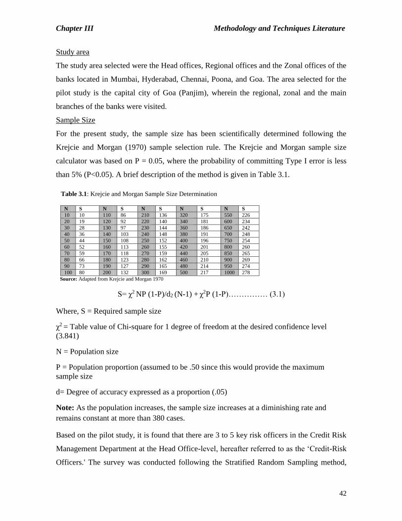
Chapter III Methodology and Techniques Literature
42
Study area
The study area selected were the Head offices, Regional offices and the Zonal offices of the
banks located in Mumbai, Hyderabad, Chennai, Poona, and Goa. The area selected for the
pilot study is the capital city of Goa (Panjim), wherein the regional, zonal and the main
branches of the banks were visited.
Sample Size
For the present study, the sample size has been scientifically determined following the
Krejcie and Morgan (1970) sample selection rule. The Krejcie and Morgan sample size
calculator was based on P = 0.05, where the probability of committing Type I error is less
than 5% (P<0.05). A brief description of the method is given in Table 3.1.
Table 3.1: Krejcie and Morgan Sample Size Determination
N S N S N S N S N S
10 10 110 86 210 136 320 175 550 226
20 19 120 92 220 140 340 181 600 234
30 28 130 97 230 144 360 186 650 242
40 36 140 103 240 148 380 191 700 248
50 44 150 108 250 152 400 196 750 254
60 52 160 113 260 155 420 201 800 260
70 59 170 118 270 159 440 205 850 265
80 66 180 123 280 162 460 210 900 269
90 73 190 127 290 165 480 214 950 274
100 80 200 132 300 169 500 217 1000 278
Source: Adapted from Krejcie and Morgan 1970
S= χ2 NP (1-P)/d2 (N-1) + χ2P (1-P)…………… (3.1)
Where, S = Required sample size
χ2 = Table value of Chi-square for 1 degree of freedom at the desired confidence level
(3.841)
N = Population size
P = Population proportion (assumed to be .50 since this would provide the maximum
sample size
d= Degree of accuracy expressed as a proportion (.05)
Note: As the population increases, the sample size increases at a diminishing rate and
remains constant at more than 380 cases.
Based on the pilot study, it is found that there are 3 to 5 key risk officers in the Credit Risk
Management Department at the Head Office-level, hereafter referred to as the ‘Credit-Risk
Officers.' The survey was conducted following the Stratified Random Sampling method,

Chapter III Methodology and Techniques Literature
43
with two strata of public and private banks. The present study has undertaken 21 public
sector banks and 18 private banks in a sample. Therefore the population of our study is
(21x5) = 105 Credit Officers in case of Public banks, and (18x3) = 54 Credit Risk Officers
in case of private banks. Thus the total population of the present study comprises 159
Credit-Risk Officers. Table 3.1 shows that 113 Credit-Risk Officers would be an
appropriate sample considering a population size of a maximum of 160 Credit-Risk
Officers.
In order to collect data, around 140 questionnaires were distributed through Google Forms
and as well as in-person to the Credit-Risk Officers of the banks. As many as 24
respondents did not reply to the questionnaire due to their busy schedule, providing us with
an 83 percent response rate. Based on the 116 responses generated, the generalisations have
been formulated. The proportion of the sample between public and private banks is 2:1
based on the number of credit risk officers in public and private banks comprising 77 and
39 Credit-Risk Officers of Public and private banks.
The Data Collection Instrument
The data collection instrument was designed based on previous studies, who perform
similar studies but in a different environment. This instrument is similar but not identical,
having been revised after taking into account the environment and opinions of experts. The
questionnaire was sent in electronic and physical form based on the location of the
respondent. The respondents were asked scale based questions on a five-point Likert scale
ranging from 1-5. The questionnaire consists of three sections mentioned in table 3.2
Table 3.2: Information related to various sections in the questionnaire
Section I Demographic Profile
Section II Determinants of Credit Risk management Practice
Section III Preparedness in Basel III Implementation Source: Researchers Compilation based on a questionnaire
3.2.1.2 Content Validity Index (CVI) and Reliability
The content validity index was computed to provide evidence of the validity of contents in
the questionnaire and to assess the necessity of questions. The ratings of items were done
by the six experts on three factors, such as relevance, clarity and simplicity. These experts
were selected from the banking and the academic sectors. The criteria outlined by Yun and

Chapter III Methodology and Techniques Literature
44
Ulrich (2002) were used as a reference point in selecting the panel experts. In this study,
four experts were taken from banking sectors. These four experts are the regulators who
visit the local RBI office and have more than ten years of experience, while two experts
were taken from the academics holding a doctoral degree in the banking area and have
published papers in the same area. The expert’s opinion was analyzed using a quantitative
method such as Content Validity Index (CVI) to decide the quality of items. The minimum
CVR for each item to be considered as acceptable was 0.75 for a one-tailed test at the 95%
confidence level, assuming that a minimum of 8 judges was used for the study
(Lawshe,1975).
Table 3.3: CVI score calculated based on nine items from the responses of six experts
Q. N
o
Co
nstru
ct
no
.
Relev
ancy
(Sco
re)
Clarity
(Sco
re)
Sim
plicity
(Sco
re)
Resu
lts
II - 6 4 33.33 66.67 33.33 Dropped
5 50 66.67 33.33 Dropped
6 83.33 33.33 33.33 Changed
II - 8 1 33.33 66.67 33.33 Dropped
4 83.33 33.33 33.33 Changed
5 50 66.67 33.33 Dropped
6 33.33 33.33 66.67 Dropped
II - 10 33.33 50 33.33 Dropped
IV - 4 50 33.33 33.33 Dropped
Source: Authors calculations based on responses from appendix table A.1
Table 3.3 shows the CVI for nine items from the data collection instrument. The seven
items [Construct no. II-6(4), II-6(5), II-8(1)1, II-8(5), II-8 (6), II-10 and II-4] from the
instrument do not meet the criteria fixed for the study; therefore based on the CVI index
these items were dropped. Four experts suggested minor revisions regarding the clarity or
wording of two items [Constructs no. II – 6 (6) and II-8 (4)] which were incorporated into
the data collection instrument.
3.2.1.3 Pilot Study
The questionnaire was first tested through a pilot study by taking the responses from ten
public banks and eight private banks from the capital city of Goa (Panjim), wherein the
regional, zonal and the main branches of the banks were visited. The pilot study helped the

Chapter III Methodology and Techniques Literature
45
researcher to understand the overview of the Credit Risk Management Department
(CRMD), level of preparedness for implementation of Basel III norms, location of the
zonal, regional and head offices. Further, necessary modifications were made in the
questionnaire based on the responses of respondents from the pilot study. Finally, the
questionnaire was revised and restructured to meet the objectives of the study.
3.2.2 Secondary Source
The secondary data is collected from various sources such as audited statements of
individual banks and RBI websites, various publications of RBI like statistical tables, and
reports. The data is also collected from reputed data sources such as Centre for Monitoring
Indian Economy (CMIE) and Indiastats.com. The present study analysed data for thirteen
years between 2004-05 and 2016-17. The data period consists of two phases, the pre-
implementation and the post-implementation phase of Basel II and Basel III norms. This is
the period where the Basel committee put norms on the banks in the form of minimum
capital requirement, the supervisory review process, market discipline, capital buffers, etc.
The effect of all these norms is reflected in the financial statements of the banks, which are
more reliable and will reduce measurement errors.
In the present study, banks are selected as sample, because the financial data of banks are
taken from publicly available financial statements, which are more reliable and will reduce
measurement errors. Another reason is, banks are subject to many regulations and financial
statements are monitored by outsiders such as creditors, depositors, RBI (Reserve Bank of
India), SEBI (Securities Exchange Board of India), Tax Authorities, etc. The type and the
number of banks are selected based on the availability of data and the consequences of time
limitations. The secondary data is collected for the second objective on 44 Indian banks,
consist of 21 public sector banks, 18 are the private banks and five are the non-working
banks. However, for the other objectives, data about nonworking banks was not relevant;
hence for these objectives, the sample taken is 39 commercial banks (21 public banks and
18 private banks).

Chapter III Methodology and Techniques Literature
46
3.3. Hypotheses of the study
Based on the objectives of the study and the comprehensive review of the literature the
following hypotheses have been framed. The first objective of the study tests the significant
impact of the determinants affecting CRMP and compares them between public and private
banks in India. The Ordinary Least Square (OLS) regression model is used to test the
following null hypothesis:
H01: There is no significant statistical impact of credit risk determinants on their respective
Credit Risk Management Practices (CRMP), of /between public and private banks in India.
A study by Al-Tamimi (2007) showed that understanding risk and risk management, risk
monitoring and reporting and credit risk analysis has a positive relationship with risk
management practices. A conceptual study by Rosman (2009) found a positive relationship
between the RU, RI, RAA and RMC on the RMP of banks. Another study conducted by
Nazir et al. (2012) revealed that risk analysis, risk monitoring and understanding risk and
risk management are positively significantly contributing to risk management practices of
Islamic and conventional banks operating in Pakistan. A study by Jorge and Ngahu (2017)
shows that risk identification is positively significant to influence the CRMP. These studies
are conducted other than India and the above hypothesis is framed in context to Indian
banks. The Indian banks reflect unhealthy scenarios of NPA’s, which may be due to
improper CRMP. Therefore, the hypothesis states no statistical impact on the determinants
in improving CRMP.
The above hypothesis also states, no difference in the determinants of CRMP between
public and private banks in India. This hypothesis supports the institutional theory, as the
theory claims that due to the presence of uniform rules and regulations by all the banks, it
will set uniform conditions of actions triggering risk management practices highly
homogeneous in banks. The identical regulatory pressures, norms, and practices will bring
uniformity in the CRMP of all the banks; hence there may not be a statistical difference in
the determinants of CRMP between public and private banks.

Chapter III Methodology and Techniques Literature
47
The present study also compares the lending ratios between and amongst the public and
private banks based on the following null hypothesis of independent sample t-test and
ANOVA.
H02: There is no statistical difference in the lending ratios between and amongst the public
and private banks in India.
The above hypothesis states that the lending ratios mentioned above are the same for public
and private banks in India, on the ground that both these banks perform a similar function
of accepting deposits for lending; therefore, they undertake a huge credit risk. This will lead
to uniformities in the ratios of public and private banks.
The lending ratios of all the public banks will be in par with the other banks in the public
sector group, as also the case of the private sector group. Due to this, all the public sector
banks and private banks will follow a uniform procedure before sanctioning the loan and
comes under a consistent regulatory regime. Therefore the mean lending ratios of all the
public and private banks will be at the same level; hence the above null hypothesis of
ANOVA states that all the public sector banks and private bank group means are equal.
This study also covers a comparison of financial ratios between public and private banks
based on the following null hypothesis of Independent t-test:
H03: There is no statistical difference in the financial ratio (liquidity, profitability and
leverage) between the public and private banks in India.
The difference in these variables may not arise because both the banks belong to the same
industry and performing similar functions, and comes under the uniform regulatory regime
of RBI. Therefore there may not be a difference in the financial ratios between public and
private banks.
This study tries to seek the difference in the bankruptcy scores between public and private
banks in India and the difference in the original and the recalibrated model, with the aid of
Independent sample t-test. Following is the null hypothesis for the same.
H04: There is no statistical difference in the bankruptcy scores using the original and the
recalibrated bankruptcy models for banks, and between public and private banks in India.

Chapter III Methodology and Techniques Literature
48
The difference in these models may not arise, as both models are using the same accounting
variable to arrive at a score. Similarly, there may not arise, a difference in the bankruptcy
score between public and private banks, due to the similarity in the lending function
performed by both the banks. Both these banks are carrying the risk of default by the
borrower and therefore have an equal chance of becoming bankrupt due to non-payment by
the borrower.
This study explains the Basel III preparedness (BP) of public and private sector banks in
India, in terms of understanding the factors influencing BP. These factors are Anticipated
Benefit (AB), Anticipated Cost (AC), Anticipated Impact (AI) and Expected Challenge
(EC). The Multiple linear regression model is used to test the following null hypothesis:
H05: There is no statistical impact of factors such as Anticipated Benefit, Anticipated Cost,
Anticipated Impact and Expected Challenge on the Basel III Preparedness for and between
the public and private banks in India.
The hypothesis states that the factor AB, AC, AI and EC are not the influential factors for
Basel III preparedness. This hypothesis is framed based on the assumption of the
fundamental uncertainty of the Legal Theory of Finance (LTF). The theory states that, if the
cost of enforcement of norms exceeds the benefit it gains, then the cut down of these norms
will be a priority for the survival of banks. This theory is related to understanding the Non-
contributory factors for the Basel III preparedness by the banks. The factors will be non-
contributory to BP when there is no impact of these factors on BP.
The above hypothesis also states the uniformity in the preparations of Basel III norms by
public and private banks in India. This hypothesis is framed based on the uniform schedule
or the phase-in arrangement of the Basel III norms given by the RBI to the Indian banks.
This schedule makes the uniform enforcement of the Basel III norms by public and private
banks. Therefore both these banks are undertaking similar steps for the preparations of
Basel III norms; hence there may not be any difference in the preparations of Basel III
norms by public and private banks in India.

Chapter III Methodology and Techniques Literature
49
This study explains the compliance of Basel III ratios of public and private banks with the
minimum required ratio prescribed by RBI in Basel III, based on the following hypothesis
of one sample T-test.
H06: The mean actual Basel III compliance ratios of public and private banks in India are
lower or equal to the minimum Basel III ratio prescribed by RBI.
The actual Basel III requirement ratios of public banks and private banks could be lower
because, historically banks were maintaining a low provision coverage ratio, as the Indian
banks have a high proportion of NPAs that are not provided for the capital.
Further, this study comprises of comparison of the Basel III capital ratios between public
and private banks in the pre-implementation phase and also in the post-implementation
phase of the Basel III period using an Independent sample T-test.
H07: There is no statistical difference in the mean Tier I, Tier II and Capital Adequacy
Ratio between public and private banks in India in the pre-implementation and post-
implementation phase of Basel III norms.
The pre-implementation phase covers the period from 2009-2013 and in this phase, banks
were following Basel II norms. Similarly, the post-implementation phase covers the period
from 2014 -2018 and in this period, banks were following Basel III norms. Due to the
implementation of these norms by the banks, the difference in the above ratios may not be
there in this period between public and private banks.
Lastly, this study covers a comparison of Basel III capital ratios before and after the
adoption of Basel III norms, with the help of the following hypothesis of paired T-test
H08: There is no statistical difference in the mean Tier I, Tier II, Capital Adequacy Ratio
among the public and private banks in India before and after the adoption of the Basel III
norms.

Chapter III Methodology and Techniques Literature
50
The significant difference in these ratios may not arise for public banks, because
historically, these banks were maintaining adequate capital and controls the majority share
in the market, possessing good capital health. Therefore there may not be any difference in
the above ratios of public banks before and after the adoption of Basel III norms.
Similarly, the difference in capital ratios may not arise in the case of the private banks, as
these banks were always playing the precautionary role before granting a loan to the
business community and therefore, the NPA’s of these banks were always less compared to
NPA’s of public banks. Further, these banks were maintaining higher capital ratios, even
before the adoption of Basel III norms as per observation to appendix table A.60 (CAR).
3.4. Statistical Tools
The present study used a variety of statistical tools for data validity, data description, and
data analysis. These tools are the following:
3.4.1 Principal Component Analysis (PCA)
PCA is a data compression tool that is utilized to decrease huge sections of variables into
small sections, that still contains most of the common information in the larger set. In the
present study, PCA is used to determine the factors influencing Credit Risk management
Practices (CRMP) of banks using the data generated from section II of the questionnaire
(Appendix table A.2). It is used on 31 statements of the questionnaire. In this study, the
selection of the variable is made based upon Eigenvalues, visualization of the Scree plot,
and Rotated Component Matrix.
3.4.2 Reliability Test
The reliability of the data collected on the Likert five-point scales in the questionnaire was
checked using Cronbach's alpha reliability coefficients, which measure the consistency with
which respondents answer the question within a scale. In the present study, for all the
constructs, the reliability coefficients are greater than 0.7, which concludes that the data
collected by the researcher is reliable and can be used for further analysis.

Chapter III Methodology and Techniques Literature
51
3.4.3 Descriptive Statistics
The descriptive statistics provides summary of variables in terms of percentage, frequency,
mean, median, standard deviation, kurtosis, skewness, minimum, and maximum value, to
organize and summarize data and to describe the characteristics of the sample. The data
with respect to the determinants of CRMP and dimensions of Basel III preparedness of
public and private banks in India is described in terms of mean, median, standard deviation,
kurtosis, skewness and range, minimum and maximum values. This helps us to provide a
summary of all variables concerning the respondent. The data concerning financial ratios is
described in terms of mean, maximum, minimum and standard deviation in the appendix
table (A.22-A.39) to understand the trend analysis of cross-sectional and time-series data.
3.4.4 Ratio Analysis
The ‘Lending Ratios’ such as Gross NPA to Gross Advance Ratio, Net NPA to Net
Advance Ratio, Total Loan to Total Asset, Total Loan to Total Deposit, Total Loan to Total
Equity, Provision for NPA to NPA, Capital Adequacy Ratio and Return on Asset are used
in the present study. Further, 'Financial Ratios' are used to measure the profitability,
liquidity and leverage position of the public and private banks in India. Profitability is
measured using Earnings before Interest and Tax to Total Assets, Earnings Before Interest
and Tax to Current Liability, ROA and Total Income to Total Asset. The Liquidity is
measured using Working Capital to Total Asset, Current Asset to Current Liabilities, while
the Leverage is measured using Retained Earnings to Total Asset, Market Value of Equity
to Total Liability and Total Deposit to Total Asset. The need for measurement of the above
variables arises as they act as a basis to determine the bankruptcy score.
3.4.5 Pearson Correlation Coefficient
Pearson’s Correlation Coefficient is used to find the relationship between financial ratios
used to measure liquidity, profitability and leverage. It is also used to meet the assumption
of multiple linear regression and OLS regression.

Chapter III Methodology and Techniques Literature
52
3.4.6 Parametric Test and Non-parametric Tests
An independent sample t-test is conducted to compare the difference in credit risk
determinants of CRMP, lending and financial ratios, bankruptcy scores, Basel III
preparedness and the Tier I, Tier II and CAR between public and private banks in India.
This test is also used to compare the difference in the bankruptcy scores between the
original and the recalibrated bankruptcy models. The test of ANOVA is used on lending
ratios to find a significant difference amongst the banks. Further, a post hoc test is
conducted to find which bank reveals a statistically significant difference in the group. One
sample t-test is used to compares the actual Basel III ratios of public and private banks with
minimum ratios prescribed by RBI while paired t-test is run to determine the significant
mean difference in the mean tier I cap ratio, tier II cap ratio, and the capital adequacy ratio
in the pre-implementation and post-implementation phase of Basel III norms. Non-
parametric test such as Mann-Whitney U-test is used for comparing the financial ratios, as
the data was found to be following the non-normal distribution
3.4.7 Regression Analysis
Regression Analysis is a powerful statistical method that allows the examination of the
relationship between two or more variables. In the present study, two types of regressions
are used, such as Ordinary Least Square (OLS) regression and Multiple Linear Regression.
The Ordinary Least Square (OLS) regression is used to determine the statistical impact of
the credit risk determinants on CRMP. The result of the PCA shows that CRMP is
dependent on four credit risk determinants.
Thus the multiple regression equation of CRMP is as follows:
CRMP = f (CRU+CRI+CRAA+CRMC) ----------------- (3.1)
Where the independent variable Credit Risk Management Practices (CRMP) are a function
of Credit Risk Understanding (CRU), Credit Risk Identification (CRI), Credit Risk
Assessment and Analysis (CRAA) and Credit Risk Monitoring and Control (CRMC). All
the assumptions required to run the regression, such as testing of linearity, testing of
independence of observation, testing for outliers, testing for Homoscedasticity, testing of
normality and multicollinearity test were checked before running a regression.

Chapter III Methodology and Techniques Literature
53
The second type of regression used in the present study is the Multiple Linear Regression.
This regression allows the researcher to determine the overall fit of the model and the
relative contribution of each of the total variance explained. This regression is used to
recalibrate the bankruptcy models. These equations are:
1. Recalibrated Equation of Altman Model
Z-scores = β+βX1+βX2+βX3+βX4......................................... (3.2)
Z-scores = 2.22 + 0.754X1 + 0.036X2 + 0.199X3 + 0.239X4
Where X1= Working capital/Total assets, X2= Retained earnings/Total assets, X3=
Earnings before interest and taxes/total assets, X4= Market value equity/Book value of
Total liabilities and Z= overall index.
2. Recalibrated Equation of Springate Model
S-scores = β +β1X1+β2X2+β3X3+β4X4........................ (3.3)
S-scores = 0.093 + 1.37X1 + 7.124X2 + 0.585X3 - 1.988X4
Where X1= Working capital/Total assets, X2= Earnings before Interest and Tax/Total
assets, X3= Earnings before interest and taxes/Current Liability, X4= Total Income/Total
Asset, and S= overall index.
3. Recalibrated Equation of Zmijewski Model
X-scores =β +β1X1+β2X2-β3X3.............................. (3.4)
X-scores = -2.534 - 3.79X1 + 4.246X2 - 0.081X3
Where X1 = Return on Asset (ROA), X2 = Total deposit to Total Asset, X3 = Current Asset
to Current Liabilities and X-Score = overall index.
4. Recalibrated Equation of Grover Model
G-scores =β +β1X1+β2X2-β3X3 ............................ (3.5)
G-scores = 0.074 + 1.65X1 + 3.09X2 - 0.014X3
Where X1= Working capital/Total assets, X2= Earnings before Interest and Tax/Total
assets, X3= Return on Asset (ROA) and G-Score = overall index.

Chapter III Methodology and Techniques Literature
54
The recalibrated model consists of the same variable as the original model, but the
coefficients differ. To develop a recalibrated model, all the assumptions required for the
regression were checked. These assumptions are correlation coefficients, independence of
errors, multicollinearity, homoscedasticity, normality, normality of residuals, presence of
outliers and data fit of the model.
The multiple linear regression is also used to measure the factors impacting the impact of
the Basel III preparedness. The conceptual framework states that Basel III Preparedness
(BP) is dependent on four factors, such as AB, AC, AI, and EC. Thus the regression
equation of Basel III Preparedness is as follows:
BP= f (AB+AC+AI+EC).............. (3.6)
Where BP= Basel III Preparedness, AB = Anticipated Benefit, AC = Anticipated Cost, AI
= Anticipated Impact and EC = Expected Challenges.
3.4.8 Robust Test
The robust test is conducted to measure the financial health of the bank in the year 2017.
This test was conducted, taking into account profitability and asset quality as a variable.
These variables are measured using a proxy to a variable such as Return on Asset (ROA)
and Net NPA to Net Advances ratio, respectively, for the year 2017. Thus for the robust
test ROA and Net NPA to Net Advance ratio for the current year 2017 is considered.
3.5. Descriptions of Bankruptcy Models
3.5.1 Altman Z-Score Model -1968
In the year 1967, Edward Altman - Finance Professor of Leonard N. Stern School of
Business of New York University developed the financial model in the year 1967 to predict
the likelihood of bankruptcy of a company. His work was based on the notion that the
univariate prediction model served in most cases as an indicator and not as a predictor of
bankruptcy. Before the development of the Altman -1968 model, he tested 22 tentative
variables as a significant predictor of bankruptcy from the five areas such as liquidity,
profitability, leverage, solvency and activity. Finally, based on five variables, he developed
a Z-score model. In his model, he used 33 bankrupt and 33 non - bankrupt firms covering a

Chapter III Methodology and Techniques Literature
55
period from 1946 -1965. His model gains an accuracy rate of 94%. This model was applied
by Nandi and Chaudhary (2011), Popker (2013), Sharma and Mayanka (2013), Chotalia
(2014), Pradhan (2014), Vaziris and Bhuyan (2012), Lin (2015) and Maina and Sawka
(2017). The model developed a following equation with zones of discrimination
Z = 1.2X1 + 1.4X2 + 3.3X3 + 0.6X4 + 1.0X5 ………..(3.7)
Where X1 = Working capital/Total assets, X2 = Retained earnings/Total assets, X3=
Earnings before interest and taxes/Total assets, X4 = Market value equity/Book value of
total liabilities and Z= overall index.
Zones of discrimination
Z > 2.99 = “Safe” Zone
1.81 < Z < 2.99 = “Gray” Zone
Z < 1.81 = “Distress” Zone
Extension of Z-score Model -1993
Z-score was re-estimated based on the other databases for private manufacturing
companies, non-manufacturing companies, and service companies. The Z-score model for
the service companies uses four variables to discriminate between obligors. These variables
are – liquidity, leverage, profitability, and solvency. These variables are measured with the
help of the following ratios:
An equation for service industries as per Z-score Model -1993
Z = 6.56X1+ 3.26 X2+6.72 X3+1.05 X4 …………………………………………… (3.8)
Where X1= Working capital/Total assets, X2 = Retained earnings/Total assets, X3=
Earnings before interest and taxes/total assets, X4 = Market value equity/Book value of
Total liabilities and Z= overall index.
The ‘Working capital/Total assets (WC/TA)’ ratio measures the liquidity of the firm’s
assets. Altman considers that a firm with heavy operational losses will have diminishing
current assets compared to the total assets. The second ratio ‘Retained earnings/Total assets
(RE/TA)’indicates the ability of the firm to earn profit through retained earnings and
measure of the cumulative profitability in time. Altman (2000) notes that the retained

Chapter III Methodology and Techniques Literature
56
earnings account can be influenced by certain corporate strategies like a reorganization or
dividend declarations. The third ratio ‘Earnings before interest and taxes/Total assets’
measures the profitability of the business and is an indicator of effectiveness of banks in
using its assets to generate earnings before the payment of contractual obligations. The last
ratio ‘Market value equity/book value of total liabilities’ indicates the proportion of owners
fund to the long term debt. A high value of ratio depicts a firm’s aggressiveness in
financing its growth with debt. This rate shows the amount by which the value of the assets
of the firm can fall before the liabilities surmount the assets, and thus the firm is insolvent.
Based on the results of Z- score, banks may be classified into different zones shown in
Table 3.4: Bases of discrimination of Altman Model
Situation Z - score Zones
I 1.1 or less Distress zone
II 1.1 to 2.6 Grey area
III 2.6 or more Safe zone
Source: Secondary data
3.5.2 Springate Model - 1978
The Springate model introduced by Gordon LV Springate in the year1978 and is a
revolution of the Altman model. According to Cantemir (2014) it is a strong alternative to
Altman's research. This models initially tested 19 financial ratios that have been frequently
used by firms and finally chose four financial ratios to be used to determine whether the
company is said to be either a healthy company or potentially insolvent. The Springate
model examines insufficient liquidity, excess debt, insufficient sales and lack of profit as
the factors to determine the health of firms. Springate used 40 companies as the sample for
this research. Springate test shows that the model has an accuracy rate of 92.5%. A study
by Arasu (2013), reports that the Springate model was tested using forty companies and
achieved a bankruptcy prediction rate of 92.5%. The Springate -1978 study formulated a
equation as follows:
S= 1.3X1 + 3.07X2 + 0.66X3 + 0.4X4 …………………….. (3.9)

Chapter III Methodology and Techniques Literature
57
Where X1 = Working capital/Total assets, X2 = Earnings before Interest and Tax/Total
assets, X3 = Earnings before interest and taxes/Current Liability, X4 = Total Income/Total
Asset, and S= overall index.
In the Springate S-score, the first ratio which is the ‘working capital divided by total asset’
measures the liquid asset concerning the firm’s size. The second ratio ‘profit before interest
and taxes divided by total assets’ estimates the cash supply available for allocation to
creditors, the government and shareholders. This ratio is a measure of an organization's
operating efficiency separated from any leverage effects and it is a true depiction of asset
production (Pandey 2011). The third ratio ‘profit before taxes divided by current liabilities’
estimates the cash supply available from the operation, for honoring the short-term
obligations of the firm. Last ratio ‘sales divided by total assets’, measures the capital
turnover. Financial analysts find the Springate model useful as it can increase the power of
decision for investors and suppliers of financial resources to sustain financial markets
(Security Exchange) for ensuring the allocation of optimal financial resources (Arasu et al.
2013). Table 3.5 shows the zones of discrimination for the Springate model.
Table 3.5: Bases of discrimination of Springate Model
Outcome (S-score) S = ≤ 0.862 “Financial Distress”
≥ 0.862 "safe Zone"
Source: Secondary Data
3.5.3 Zmijewski Model - 1984
A study by Mark E. Zmijewski (1984), created a financial distress prediction model based
on Ohlson (1980) work popularly known as Zmijewski model. Zmijewski used the Probit
method to predict bankruptcy. The Probit regression is suitable when the dependent
variable is qualitative and the independent variables are quantitative. During the
development of model Zmijewski’s took external factors, such as industry sector, size of
the company, economic cycle, etc. Therefore, he used all non-financial, non-service and
non-public administration firms listed on American and New York Stock Exchange from
1972-78. His sample consists of 40 bankrupt and 800 non-bankrupts firms. The original

Chapter III Methodology and Techniques Literature
58
models reported an accuracy rate of 98.2%. This model uses variables such as profitability,
leverage and liquidity. This model arrived the following equation:
X - Score = - 4.3 - 4.5X1 + 5.7X2 - 0.004X3 ………………….. (3.10)
Where X1 = Return on Asset (ROA), X2 = Total deposit to Total Asset, X3 = Current Asset
to Current Liabilities and X-Score = overall index.
Based on the results of model, X-Score values obtained are divided into two classes. If the
X-score is negative (X - Score < 0), then the company is classified in a healthy condition.
Conversely, if the X-score is positive (X-Score ≥0) then the company is classified under
financial distress. It is noted that X-score can be converted to bankruptcy probability using
the expression - 1/1+ε-1.8138Zm
Probit models use a latent variable Y* that ranges from negative infinity to positive infinity.
The cumulative standard normal function G transforms the latent variable Y* into a
predicted Y value between 0 and 1.
Pr(𝑌)=𝐺(𝑌∗)=𝐺(𝛽0+𝛽1𝑥1+𝛽2𝑥2+⋯+𝛽𝑘𝑥𝑘 )……….(3.11)
The estimated coefficients from the Probit regression are difficult to interpret because they
measure the change in the latent variable, not Y itself. The marginal effects are a more
useful way to measure the magnitude of the estimated coefficients.
Table 3.6: Bases of discrimination of Zmijewski Model
Outcome (X-Score)
X-score < 0 = ‘Safe’
>0 = ‘Financial Distress’
Probability (X-score) = ≤ 0.5 ‘Safe’
> 0.5 ‘Financial distress’
Source: Secondary data
The Probit model of Zmijewski is beneficial in comparison with MDA because the Probit
function maps the value to a probability bounded between 0 and 1, which is easy to
interpret. In statistical matters, the Zmijewski model defines bases of discrimination as in
case of a p-value or X - score that is equal or greater than 0.5 is classified as ‘Financial
distress’ and companies having a p-value that is lower than 0.5 are classified as ‘Safe’
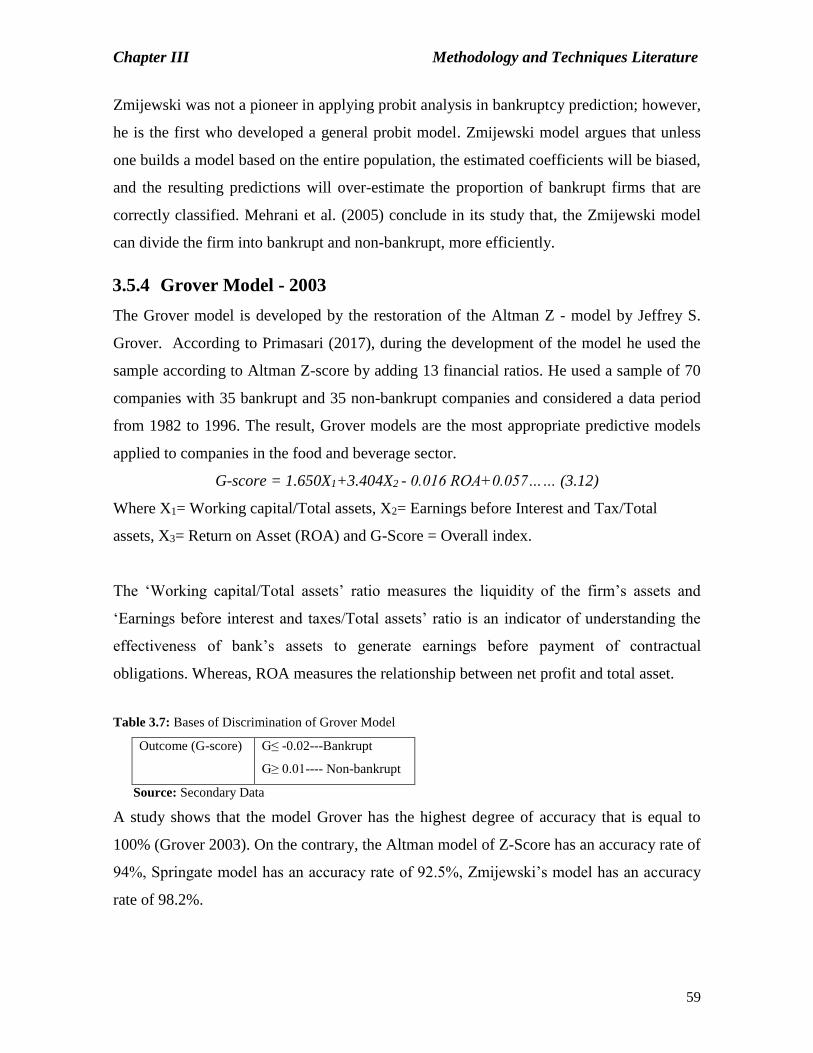
Chapter III Methodology and Techniques Literature
59
Zmijewski was not a pioneer in applying probit analysis in bankruptcy prediction; however,
he is the first who developed a general probit model. Zmijewski model argues that unless
one builds a model based on the entire population, the estimated coefficients will be biased,
and the resulting predictions will over-estimate the proportion of bankrupt firms that are
correctly classified. Mehrani et al. (2005) conclude in its study that, the Zmijewski model
can divide the firm into bankrupt and non-bankrupt, more efficiently.
3.5.4 Grover Model - 2003
The Grover model is developed by the restoration of the Altman Z - model by Jeffrey S.
Grover. According to Primasari (2017), during the development of the model he used the
sample according to Altman Z-score by adding 13 financial ratios. He used a sample of 70
companies with 35 bankrupt and 35 non-bankrupt companies and considered a data period
from 1982 to 1996. The result, Grover models are the most appropriate predictive models
applied to companies in the food and beverage sector.
G-score = 1.650X1+3.404X2 - 0.016 ROA+0.057…… (3.12)
Where X1= Working capital/Total assets, X2= Earnings before Interest and Tax/Total
assets, X3= Return on Asset (ROA) and G-Score = Overall index.
The ‘Working capital/Total assets’ ratio measures the liquidity of the firm’s assets and
‘Earnings before interest and taxes/Total assets’ ratio is an indicator of understanding the
effectiveness of bank’s assets to generate earnings before payment of contractual
obligations. Whereas, ROA measures the relationship between net profit and total asset.
Table 3.7: Bases of Discrimination of Grover Model
Outcome (G-score) G≤ -0.02---Bankrupt
G≥ 0.01---- Non-bankrupt
Source: Secondary Data
A study shows that the model Grover has the highest degree of accuracy that is equal to
100% (Grover 2003). On the contrary, the Altman model of Z-Score has an accuracy rate of
94%, Springate model has an accuracy rate of 92.5%, Zmijewski’s model has an accuracy
rate of 98.2%.
Chapter IV Determinants of Credit Risk Management Practices
60
Chapter IV
Determinants of Credit Risk Management Practices
4.1. Introduction
The banking sector is the mainstream of capital inflows and outflows of the economic
system of the country. The banking sector in an Indian economy is undergoing a process of
change, driving them to pose a higher risk. Therefore, there is a critical need for risk
management in this sector. Risk management is understood as a set of departments or
bodies concerned with identifying, assessing, mitigating and reporting risk. The risk
management is an ongoing process, which is highly dependent on the volatility of the
internal and external environment of the banks. Some of the risk is at the micro level, such
as the negative effects of the recession, political interference, natural disasters, and some
are at the macro level such as credit risk, liquidity risk, foreign exchange risk and
operational risk.
The banks face four types of risk such as credit risk, market risk, liquidity risk, and
operational risk. These four risks have a manifold effect on the performance of the banks
however, the magnitude and the extent of loss caused by credit risks are more severe and
can lead to bank failures. Thus, from amongst the above mentioned risk, credit risk is the
most significant risk, as it has a substantial impact on the financial health of the banks.
According to Afande (2014) the credit risk problem often begins right at the loan
application stage and increases further at the loan approval, monitoring and controlling
stages, especially when CRM guidelines in terms of policy an strategies/procedures for
credit processing do not exist are weak or incomplete. Due to this reason, the management
of credit risk is the most prominent strategy banks need to adopt for survival. Credit risk
management is a broad term, which includes principles, processes, and practices adopted by
the banks. The principles and processes guide the adoption of effective Credit Risk
Management Practices (CRMP). Considering this fact, the present study focuses on
effective CRMP. It is understood that “CRMP means establishing a suitable credit risk
management environment by understanding, identifying, assessment and monitoring the
credit risk.”

Chapter IV Determinants of Credit Risk Management Practices
61
The significance of effective credit risk management practices has increased with time
basically due to prior global meltdown. Further, the credit risk is not only triggered in the
banks due to micro factors but also due to macro factors. It is a problem not just restricted
to national boundary, but the effect of improper credit risk management is spread all over
the world. Thus, not only the country’s economy is affected due to credit risk, but there is a
world economy meltdown due to credit risk. The proliferation of 2008 crisis worldwide
triggered the attention of the researcher towards better credit risk management practices of
the banks, as the major cause of the financial crisis is ineffective credit risk management
practice. In recent years, risk management in banking institutions has got substantial
importance and has become the center debate after the global financial crisis (Ishitiq 2015).
Besides, a study by Rehman (2016), states that risk management is getting more attention,
especially after the credit crunch in 2007 to 2009. Thus, owing to the increasing NPA’s,
CRMP has jumped to the forefront of credit risk management activities carried out by the
banks.
The present study covers the CRMP of the public and the private banks in India to check
the extent and magnitude of variation. It is essential to acknowledge the literature, which
states that CRMP of the public and the private banks differ. This difference may be on
account of an exceptional challenge public sector banks need to face in managing credit
risk due to government control and interference. This interference the government is to
improve the scenario of the Indian economy. As per Kamat (2019), the situation of the
Indian economy reflects that the government needs to address issues such as Job creation,
NPA laden banking, falling investments, poor performance of exports, and burgeoning
deficits. This shows the need for the speedy recovery of the Indian economy along with the
revival of the automobile, banking, finance, service telecom etc. The above issues drive the
government to depend on the public sector banks for financial assistance.
The present chapter is an empirical study which summarizes the findings from the primary
data collected through a questionnaire. It aims to identify the factors (determinants)
affecting credit risk management practices, measure its individual impact and compare
them between public and private banks. This chapter consisting results and discussion is
divided into four parts. Part I explains the sample characteristics such as demographic

Chapter IV Determinants of Credit Risk Management Practices
62
profile, content validity, pilot study. Part II comprises of reliability analysis and Principal
Component Analysis (PCA). Part III consists of descriptive statistics on all the
determinants of CRMP and Pearson’s correlation coefficient. Part IV covers the regression
analysis to measure the credit risk determinants impact on CRMP. It also includes the
results of the Independent sample T-test to compare the credit risk determinants between
public and private banks in India.
4.2. Theory and Literature
4.2.1 Institutional Theory
The present study applies the Institutional Theory to find the extent of uniformity in the
credit risk determinants of CRMP between public and private banks. The Institutional
Theory describes norms, ideologies, values, which need to be uniformly followed by all to
run their organizations. The institutionalization exists when the risk management activities
in most of the institutions become highly equivalent. This equality can be attained through
the coercive isomorphic method by which political and lawfulness pressures are employed
on institutions in the forms of persuasion, direction or invitation. It is understood from the
theory that, due to regulatory pressure, enduring practices and structure will set uniform
conditions of actions triggering risk management practices highly homogeneous in banks.
According to this theory, there is a homogeneity of CRMP between public and private
banks.
4.2.2 Literature Review
Studies by Benar (2001), Rosman (2009), Purukaystha and Raul (2014), Harrie (2015),
Aven (2016) studied the historical perspectives and conceptual framework of risk and risk
management practices over a period of time. A study by Diksha and Arora (2009),
Bharadwaj (2013) and Subramanyam, et al. (2016), throws light on the weakness of
corporate governance structure of the banks and improper management of credit risk by
banks. The credit risk management policies of private banks are different from public banks
as per the studies of Thiagarajan (2011), Goel and Rekhi (2013), Kattel (2016) and
Pourkeiki (2016).

Chapter IV Determinants of Credit Risk Management Practices
63
The empirical literature is available on Risk Management Practices (RMP) and the factors
affecting the RMP. A conceptual study by Das (2005) and Rosman (2009), figures out the
theoretical model of RMP. Das (2005), in its study presented guidelines on determinants of
RMP. A study by Rosman (2009) stated the use of four determinants in understanding the
RMP. Ample literature is available specifying the empirical evidence on determinants of
RMP. A studies by Al-Tamimi & Al-Mazoorie (2002), Al-Tamimi and Al- Mazrooei
(2007), Onyano (2010), Shafiq and Nasr (2010), Nazir (2012), Hussiney (2012), Gakure
(2012), Hussain (2015) and Ishtiaq (2015), Ngoroge and Ngahu (2017), applied RMP
model on different banks in their countries.
Literature on the above studies shows that some studies used three determinants, while
other studies used seven determinants. Ishitiaq (2015) conducted a study in Pakistan and
used seven determinants. Similarly, Al Tamimi (2007), Al-Tamimi & Al-Mazoorie (2002)
conducted a study in UAE, also Hussain & Al-Ajmi, (2012) conducted a study in Bahrain
and Shafiq & Nasr (2010) conducted a study in Pakistan using five determinants. A study
conducted by Rehman (2016) in Pakistan used six determinants. A study by Ngoroge and
Ngahu (2017) used one factor i.e. Risk Identification (RI), to find its impact on the
performance of the bank. This shows that these determinants are not standard. Thus, the
present study is an extension to the above studies with a difference in terms of focusing on
credit risk, identification of the determinants using Principal Component Analysis (PCA),
and a study about Indian banks.
4.3. Data and Methods
This chapter used primary data collected through a predesigned structured questionnaire.
Before designing the questionnaire, desk research was conducted to study literature on the
available subject and to have a complete understanding of various parameters to be
included in the questionnaire. The questionnaire was tested with a content validity test
(Annexure 1) and a pilot study. In the content validity, the ratings of items were done by six
experts on three factors such as relevance, clarity, and simplicity. The result of the content
validity Index shows minor revision regarding the clarity or wording of the items and those
revisions were incorporated into the instrument. The questionnaire was answered by Credit

Chapter IV Determinants of Credit Risk Management Practices
64
Risk Officers of Banks. Most of these officers possessed an experience of more than five
years and a designation of managership as per table 4.2.
Thirty-one questions were used to find the credit risk determinants of CRMP as per
annexure table II. These thirty one statements are undertaken based on the questionnaire of
past studies such as Al-Tamimi and Al-Mazoorie (2002), Al-Tamimi and Al- Mazrooei
(2007), Onyano (2010), Shafiq and Nasr (2010), Nazir (2012), Hussiney (2012), Gakure
(2012), Hussain (2015) and Ishtiaq (2015), Ngoroge and Ngahu (2017). These thirty-one
statements were overlapping and conveyed the same meaning. These thirty one statements
were used by the above studies in their countries to find the determinants of CRMP. The
present study poses a research problem in recognising of exact determinants of CRMP
given the different factors that govern CRMP in different countries. The factors applicable
in some context/nations may not apply to Indian banks due to the difference in the
economic background and the Central Bank's policies of the country. Also, certain studies
used many determinants resulting in the problem of collinearity. Therefore a data
compression tool called PCA was used in the study to identify the credit risk determinants.
This technique could reduce the huge sections of variables into small sections that still
contain most of the common information in the larger set.
The PCA technique reduced the thirty-one statements into twenty two statements.
Assumption such as the suitability of data is measured through the Kaiser-Meyer-Olkin
(KMO) test. The KMO values range from 0 to 1. High values indicate usefulness. Both
William et al. (2010) and Parinet et al. (2004) state the data is adequate when the value is
greater than 0.5. The second assumption of PCA is used to check the Eigen value. An Eigen
value of 1 represents the variance of one variable. Another method to decide the retention
of the component is a visual inspection of the Scree plot. In the Scree plot, only those
components are retained before the last inflection point of the graph. Finally, the retention
of components is made based on Eigen value, visual inspection of Scree plot and rotated
component matrix. Based on PCA, twenty two statements were used to identify the
determinants of CRMP. Reliability analysis was used on these statements to assess the
chances of random error entered.

Chapter IV Determinants of Credit Risk Management Practices
65
Descriptive statistics (mean, median, variance in data, Kurtosis and the maximum and
minimum value) presented in Table 4.6 were used to summarize and describe the
characteristics of the sample, while the Pearson correlation coefficient was used to check
the relationship between the independent variables. Regression analysis was used in the
present study to measure the relationship between several independent variables and a
single dependent variable. The present study used Ordinary Least Square (OLS) to test the
significant impact of the dependent variable on the independent variable. OLS method is
applied in the current study because this is a well-accepted method and commonly used in
studies such as Al Tamimi and Mazoorie (2007), Shafiq and Nasr (2010) etc.
Any Assumptions required to run the ordinary least square regression such as linearity,
independence of observation, outliers, homoscedasticity, normality, normal PP-plot etc.
were checked before running a regression. An independent sample T-test was conducted to
compare the differences in CRMP of public and private banks.
.
4.4. Conceptual Framework of CRMP
Risk management is a wide term, which includes principles, process and practices. Risk
management principles are the rule of action guiding the effective implementation of the
risk management process and also a guiding force for adopting effective risk management
practices. The risk management process is a mechanism for the implementation of the
practice. Considering this fact, it is understood that the principles and processes guide the
adoption of effective Risk Management Practices (RMP). This study focuses on the
adoption of effective RMP. RMP is a broad term that includes determinants governing
RMP and the tools for measurement of credit risk.
RMP is a model comprises of four determinants such as Risk Identification, Risk
Understanding, Risk Assessment and Analysis and Risk Monitoring Control. These are
called determinants or factors because it contributes to effective RMP..

Chapter IV Determinants of Credit Risk Management Practices
66
Based on literature review, it was found that most of the studies in the past have covered all
types of risk under the Risk Management Practices (RMP). These studies are Al-Tamimi &
Al-Mazoorie (2002), Al-Tamimi and Al- Mazrooei (2007), Onyano (2010), Shafiq and
Nasr (2010), Nazir (2012), Hussiney (2012), Gakure (2012), Hussain (2015) and Ishtiaq
(2015), Ngoroge and Ngahu (2017). Further, most of the above studies show the use of five
determinants as an independent variable to arrive at a RMP model. These determinants are
Understanding Risk Management (URM), Risk Identification (RI), Risk Assessment and
Analysis (RAA), Risk Monitoring (RMC) and Credit Risk Analysis (CRA). Following is
the equation used by these studies to understand the impact of the independent variable on
the dependent variable.
RMP = f (URM+RI+RAA+RMC+CRA)…………….. (4.1)
In the above equation, RMP is a response variable that is measured using five explanatory
variables such as URM, RI, RAA, RMC, and CRA.
4.4.1 Risk Management Practices (RMP)
The RMP means establishing an appropriate risk management environment, this can be
created by developing sound policies to identify, manage and measure the risk. Thus RMP
covers the framing of policies on different aspects of risk, identification of risk and
measurement of the risk using tools and techniques.
4.4.2 Understanding Risk Management (URM)
The URM is significant for bank employees to understand the factors causing risk, to make
them vigilant about the threats of banking operations and the risks that are inherent and
exposed in their business operations. A better understanding of risk management is also
important in the bank’s activities where managing risk is one of the most important
objectives of banks. A change in the attitude and mindset of the employees will drive them
to understand that managing risk is crucial for the bank’s success.
4.4.3 Risk Identification (RI)
This variable involves the procedure of identifying threats that confront to banks and
forecasting the happening of such an event. It means deciding in advance the positive and

Chapter IV Determinants of Credit Risk Management Practices
67
negative effects of each threat and also deciding the procedure to control threat. There are
several techniques that can be used in risk identification, such as crucial observation areas
inside and outside the banks, assigning responsibilities to the employees of banks to
identify specific risks. The risk identification process is normally conducted by the risk
analyst, who estimates the likelihood of the threats and identifies the procedure to control it.
4.4.4 Risk Assessment and Analysis (RAA)
RAA classifies the different risk according to the amount of damage it possibly causes.
This classification enables the management to divide risks that are enabling threat to the
existence of the corporation from those which can only cause slight damages (Rosman
2009). In other words in RAA the bank classifies the credit risks that are threatening the
existence of firm from those, which can cause a loss to the banks. A success of the banks
depends on its ability to assess risk strategically.
4.4.5 Risk Monitoring and Control (RMC)
The main task of the risk manager is to monitor, measure and control credit risk. The risk
manager's duty includes the identification of possible events or future changes that could
have a negative impact on the bank's credit portfolio and the bank's ability to withstand the
changes. In case of risk monitoring, the key areas to examine critically is counterparty's
financial position. Therefore, risk monitoring can be used to make sure that risk
management practices are in line which will help bank management to discover mistake at
an early stage.
4.4.6 Credit Risk Analysis (CRA)
This variable focuses on credit risk, as it is the most important risk which may drive the
corporate in the state of insolvency. Therefore, a detailed analysis of this risk will improve
the RMP of banks.
The present study focuses on credit risk. The reason being, credit risk is the most important
risk as it has a direct impact on the financial health, growth and survival of a bank. Also,

Chapter IV Determinants of Credit Risk Management Practices
68
the survey results show that credit risk is ranked one by the majority of respondents as seen
in table 4.1.
Table 4.1: Results of ranks given for different types of risk based on 116 respondents
Source: Authors calculations based on data collection instrument from appendix table A.3
In the data collection instrument, the respondents were asked to give a rank from 1 to 5 to
the different types of risk mentioned in table 4.1. The above table shows that the majority
of the respondents have given 1st rank for credit risk highlighting the significance of credit
risk faced by them amongst the other types of risk. This is due to the fact that lending is the
primary business of banks, which involves huge risk in case of contractual break of the
agreement by obligors. Therefore, the present study focuses on Credit Risk Management
Practices (CRMP) rather than the Risk Management Practices (RMP).
The CRMP involves designing an environment that includes creating awareness among the
bank staff on understanding the concept of credit risk, identification of sources and areas of
credit risk, analysis and assessment of credit risk, finally, monitoring and controlling credit
risk. Based on the above aspects, the data collection instrument (Appendix A.2) covers the
statements on the same.
4.5. Results and Discussion
This chapter consists of results and discussion into four parts. Part I (Sample
Characteristics), it explains the sample characteristics such as demographic profile, pilot
study, content validity, Part II (Identification and Classification of Determinants) comprises
of reliability analysis and Principal Component Analysis (PCA). Part III (Descriptive
analysis correlation analysis) consists of descriptive statistics on all the determinants of
S. N. Types of Risk Frequency Percentage
(%)
Rank
1 Credit Risk 91 84 1
2 Operational Risk 80 74 2
3 Market Risk 74 69 3
4 Exchange rate risk 63 58 5
5 Liquidity risk 85 79 4

Chapter IV Determinants of Credit Risk Management Practices
69
CRMP and the Pearson’s correlation coefficient. Part IV (Development of OLS model)
covers the regression analysis and the results of the Independent sample T-test.
4.5.1 Sample Characteristics
The sample characteristics is explained in terms of the demographic profile of the
respondents, description of the small scale preliminary study (pilot study) and an
explanation on the quality of items on the data collection instrument.
4.5.1.1. Demographic Profile
This data was collected through a predesigned structured questionnaire run on Credit Risk
Officers of Banks. Our sample size has been scientifically determined following the Krejcie
and Morgan (1970) sample selection rule. This rule shows that 113 Credit Risk Officers
would be an appropriate sample considering a population size of maximum of 160 Credit-
Risk Officers. In order to collect data, around 140 questionnaires were distributed through
Google Forms and as well as in-person to the Credit-Risk Officers of the banks. Twenty-
four respondents did not reply to the questionnaire due to their busy schedule, providing us
with an 83 percent response rate. The proportion of the sample between public and private
banks is 2:1 based on the number of credit risk officers in public and private banks
comprising 77 and 39 Credit-Risk Officers of public and private banks. Based on the 116
responses generated, the generalizations have been formulated.
Table 4.2: The demographic profile of the 116 respondents
Attributes Frequency Percentage
Type of Bank
Public 77 66 %
Private 39 34 %
Gender
Male 70 60%
Females 46 40%
Designation
Executive management 15 12%

Chapter IV Determinants of Credit Risk Management Practices
70
Middle level management 101 88%
Length of Experience
Less than five years 40 35%
Five years and Less than ten years 71 61%
Ten Years and longer 5 4%
Source: Authors Compilation based on the data collection instrument from appendix table A.3
Table 4.2 shows that gender composition of the sample is strongly influenced by males and
the majority of the risk officers belong to middle level management. The quality of the
responses will be more reliable as most of the respondents belong to the category of
possessing more than five years of experience.
4.5.1.2. Pilot Study
The questionnaire was first tested with a pilot study by taking responses from branches,
zonal and regional offices of public banks and private banks. The area selected for the pilot
study is the capital city of Goa (Panjim), wherein the regional, zonal and the main branches
of the banks were visited. The pilot study helped the researcher to understand the overview
of the Credit Risk Management Department (CRMD), the profile of the credit risk officers,
the location of the zonal, regional and the head offices etc. Thereafter, modifications were
made in the questionnaire based on the responses of respondents from the pilot study.
4.5.1.3. Test of Content validity
The Content Validity Index (CVI) was computed to provide evidence of content validity
and to assess the necessity of questions. The ratings of items were done by experts on three
factors, such as relevance, clarity and simplicity. A panel of six content experts was asked
to rate each scale item in terms of its relevance, simplicity and clarity to the underlying
constructs. These experts were selected from the banking and academic sectors. The
expert's opinion was analyzed using a quantitative method such as Content Validity Index
(CVI) to decide the quality of items. The minimum CVR for each item to be considered as
acceptable was 0.75 for a one-tailed test at the 95% confidence level, assuming that a
minimum of 8 judges was used for the study (Lawshe, 1975). The result of the content
validity Index showed a minor revision regarding the clarity and wording of items and

Chapter IV Determinants of Credit Risk Management Practices
71
those revisions were incorporated into the instrument. The detail discussion about content
validity is done in the research methodology chapter.
4.5.2 Identification and Classification of Determinants of CRMP
The result and discussion in this section include details on Principal Component Analysis
(PCA) and reliability analysis.
4.5.2.1 Principal Component Analysis (PCA)
In order to identify the determinants, Principal Component Analysis (PCA) is used. The use
of PCA in this study allows transforming and reducing the thirty one statements into a
smaller number of components and yet retaining a significant amount of information about
variance. The preliminary step for PCA is sample adequacy. The sample adequacy is
checked with the help of the Kaiser-Meyer-Olkin (KMO) test. In the present study, the
KMO values are above 0.5, the data for the models are found adequate in their collinearity.
The Rotated Component Matrix and Eigen value methods are used to decide the retention
of components.
Table 4.3: Rotated Component Matrix calculated from 31 statements from a questionnaire
Statements
Rotated Component matrix
Component 1
CRAA
Component 2
CRMC
Component 3
CRU
Component 4
CRI
Stat.26 .984 .102 .105 .038
Stat.23 .841 .109 .158 .123
Stat.13 .783 .025 .138 .102
Stat.2 .650 .166 -.053 .114
Stat.17 .612 .102 .091 .021
Stat.15 .510 .112 .103 .031
Stat.6 .113 .743 -.023 .135
Stat.29 .123 .683 .152 .082
Stat.18 .023 .612 .123 .131
Stat.24 .012 .523 .134 .026
Stat.10 .153 .514. .152 .023
Stat.21 .153 .450 .121 .052
Stat.27 .226 -.007 .780 .142

Chapter IV Determinants of Credit Risk Management Practices
72
Stat.22 .126 .113 .674 .014
Stat.11 .111 .081 .567 .091
Stat.1 .021 .112 .468 .233
Stat.4 .056 .176 .414 .145
Stat.12 .542
Stat.8 .503
Stat.16 .433
Stat.31 .413
Stat.19 .409
Source: Authors working based on data collection instrument from appendix table 4.2
The Rotated component matrix shows the retained rotated component loads on each
variable. The result of the rotated component matrix is given in Table 4.3 indicates the
inclusion of twenty-two statements and the exclusion of nine statements.
Table 4.4: Extraction of the sum of Squared Loadings
Component Eigen
values
% of
variance
Cumulative
%
Component 1 6.23 28.31 28.31
Component 2 4.08 18.54 46.85
Component 3 3.33 15.13 61.98
Component 4 2.41 10.95 72.93
Source: Authors Computation based on appendix table 4.2
The result in the above table indicates the retention of the four components, whose Kaiser -
Eigen value obtained is above one. In other words, twenty two statements are reduced to
four components. These four components put together explained 73% of variations in the
variables. The first component captured around 28% of variations. The second component
captured around 18% of variations, while the third and fourth component captured around
15 and 10 percent variations respectively.
Application of cattle Scree plot is yet another method used to determine the components to
retain in regression. A visual inspection of the Scree plot signifies the retention of four
components to be used in the regression based on the inflection point.

Chapter IV Determinants of Credit Risk Management Practices
73
Studies such as Al-Tamimi & Al-Mazoorie (2002), Al-Tamimi and Al- Mazrooei (2007),
Onyano (2010), Shafiq and Nasr (2010), Nazir (2012), Hussiney (2012), Gakure (2012),
Hussain (2015) and Ishtiaq (2015), Ngoroge and Ngahu (2017) were used as a guidance for
labeling the components (determinants). The data in table 4.5 led to the final conclusion of
grouping and labeling of factors as follows:
1. Determinant 1 has good correlation with the statement number 26, 23, 13, 2, 17 and 15
and will be labeled as CRAA (Credit Risk Assessment and Analysis).
2. Determinant 2 has good correlation with the statement number 6, 29,18,24,10 and 21
and will be labeled as CRMC (Credit Risk monitoring and Control).
3. Determinant 3 has good correlation with statement number 27, 22,11,1 and 4 and will be
labeled as CRU (Credit Risk Understanding).
4 Determinant 4 has good correlation with the statement number 12, 8, 16, 31 and 19 and
will be labeled as CRI (Credit Risk Identification).
The CRMP involves stages in a sequence such as Credit Risk Understanding (CRU), Credit
Risk Identification (CRI), Credit Risk Assessment and Analysis (CRAA) and Credit Risk
Monitoring and Control (CRMC), hence the regression equation of CRMP is as follows:
CRMP= f (CRU+CRI+CRAA+CRMC)…………… (4.2)
The original equation no 4.1 is modified as PCA has subsumed CRA in CRAA. Thus
modified equation consist of CRMP as a response variable which is measured using four
explanatory variables such as CRU CRI, CRAA, and CRMC,
Credit Risk Management Practices (CRMP)
This dependent variable is measured in the present study using six statements mentioned in
Annexure table A.3. These statements are based on the past studies such as Al-Tamimi &
Al-Mazoorie (2002), Al-Tamimi and Al- Mazrooei (2007), Onyano (2010), Shafiq and
Nasr (2010), Nazir (2012), Hussiney (2012), Gakure (2012), Hussain (2015) and Ishtiaq
(2015), Ngoroge and Ngahu (2017), who perform similar studies but in a different
environment. These statements are similar but not identical, having been revised after

Chapter IV Determinants of Credit Risk Management Practices
74
taking into account the environment and opinions of the experts. CRMP is evaluated based
on an appropriateness of banks credit risk management department, periodical preparing of
credit risk policy by bank, well documented credit risk management process that provides
guidance to the staff, assessment whether, the bank’s main objective is efficient credit risk
management, emphasis of the bank’s on recruitment of highly qualified people in credit risk
department, and whether application of Basel capital has improved the credit risk
management effectiveness in bank.
Credit Risk Understanding (CRU)
The CRU is the first independent variable used in the equation 4.2. This variable is
measured using five statements given in appendix table 4.2. These statements are related to
a common understanding among the employees of the bank and about the formal credit risk
management system, importance of managing the credit risk, understanding on different
types of risk and the risk evaluation techniques, and finally a clear understanding of bank
employees about the setup and understanding on responsibilities by the bank's staff. Every
banker, in the beginning, has to understand the portfolio of risk it has to face and basically
the credit risk it plans to take in the future. Al-Tamimi and Al- Mazoorie (2007) concludes
that a good understanding of different risk and risk management among banking employees
improves the potential of banks to manage risk. Thus, understanding credit risk is an
important determinant that can have a positive impact on the Credit Risk Management
Practices of the banks.
Credit Risk Identification (CRI)
In the present study, CRI is assessed by considering the following aspects such as
systematic procedure followed for identification of credit risk, presence of committee for
identification of credit risk, the frequency at which the changes in the credit risk is
identified by banks, a technique used for identifying credit risk. These aspects are measured
using statements from annexure table A.3.

Chapter IV Determinants of Credit Risk Management Practices
75
Credit Risk Assessment and Analysis (CRAA)
In equation 4.2, CRAA is the third independent variable used to measure impact on
CRMP.. The CRAA is measured by considering the aspects such as quantitative and
qualitative techniques followed for assessment, measurement of cost and benefit of
addressing risk, provision of well defined training for assessment of credit risk, presence of
computer based support system for assessment of credit risk to analyse the risks and the use
of standardized approach for assessment of credit risk.
Credit Risk Monitoring and Control (CRMC)
The CRMC is the last variable used in equation 4.1. This variable is evaluated by
considering six statements from annexure table A.3, such as evaluation of risk management
and control system within the bank, level of control in the bank, monitoring the
effectiveness of credit risk, evaluation of standard reporting system, monitoring of credit
limit, reporting of internal auditor, communication and reporting lines within a bank.
4.5.2.2 Reliability Analysis
The reliability of the data collected on Likert five point scales in a questionnaire from
annexure table A.3 was checked using Cronbach’s Alpha reliability coefficients, which
measure the consistency with which respondents answer the question within a scale.
Table 4.5: Reliability test on 36 statements based on 116 observations
Constructs Results
Credit Risk Understanding (CRU) 0.78
Credit Risk Identification (CRI) 0.73
Credit Risk Assessment and Analysis (CRAA) 0.81
Credit Risk Monitoring and Reporting (CRMR) 0.79
Credit Risk Management Practices (CRMP) 0.85
Source: Authors calculations based on primary data from appendix table 4.3

Chapter IV Determinants of Credit Risk Management Practices
76
Table 4.5 reports Cronbach’s alpha coefficient of all the variables is higher than the
prescribed level (0.70), indicating excellent reliability of constructs. The Coefficient of
Cronbach’s alpha for the study variables is also accordant with the results from several past
research studies, such as Al Tamimi and Mazoorie (2007) and Hussain and Al-Ajmi (2012)
4.5.3 Descriptive Statistics and Correlation Analysis
This part consists of the results and discussion on descriptive statistics of the determinants
of CRMP and correlation analysis of the independent determinants of CRMP. The
descriptive statistics describe the data in terms of mean, median, variance in data, Kurtosis
and the maximum and minimum value. The correlation analysis shows the relationship
between the dependent variable such as CRMP and the independent variable such as CRU,
CRI, CRAA and CRMC.
Table 4.6: Descriptive Statistics of 39 respondents of private and 77 respondents of public banks
Public sector banks Private banks
CRU CRI CRA CRMC CRMP CRU CRI CRAA CRMC CRMP
Mean 3.9 4.01 4.00 4.21 4.18 4.57 4.49 4.74 4.77 4.79
Median 4.4 4.2 4.16 4.33 4.66 4.8 4.6 4.6 4.83 4.83
Std. Dev 1.14 0.69 0.88 0.61 1.06 0.43 0.45 0.20 0.26 0.20
Kurtosis -0.01 -0.41 -0.11 -0.76 0.06 1.7 -0.03 1.7 0.42 2.8
Minimum 1.8 2.8 2.33 3.1 1.8 3.2 3.6 4.16 4 4.16
maximum 5 5 5 5 5 5 5 5 5 5
Count 77 77 77 77 77 39 39 39 39 39
Source: Authors calculations based on data from appendix table A.2 and A.3
The mean score of all the determinants affecting the CRMP in the case of the public sector
bank is lower than the private banks. This signifies that the contribution of the determinants
to CRMP in the case of private banks is more than the public sector banks indicating the
efficient ability of the private bank in managing the credit risk. The mean response on the
determinant CRU in the case of the private banks is higher compared to the public banks,
indicating the private banks have a good understanding of risk and risk management. The
mean score of CRAA and CRMC is also higher for the private banks signaling efficient and
effective assessment and monitoring of the credit risk. The standard deviation in the above
table shows that the variance in data in the case of private banks is lower than the public
banks. The value of kurtosis less than 3 in the above table indicates the normality of data.

Chapter IV Determinants of Credit Risk Management Practices
77
Table 4.7: The Correlation matrix calculated using 39 respondents of private and 77 respondents of public banks
Public Banks Private Banks
CRU CRI CRAA CRMC CRU CRI CRAA CRMC
CRU 1 0.403* -.063 .432* CRU 1 -0.12 .432* .253
CRI 0.403* 1 .147 .493* CRI -0.12 1 .094 .208
CRAA -.063 .147 1 .383* CRAA .432* .094 1 .490*
CRMC .432* .493* .383* 1 CRMC .253 .208 .490* 1
Source: Authors Calculation based on appendix table 2 *Correlation at 5% level of significance
The correlation analysis is conducted to meet the assumption of OLS regression. Table 4.7
shows the relationship between the independent variable, such as CRU, CRI, CRAA, and
CRMC. The relationship among the Independent variable of the banks shows the
correlation coefficient value less than 0.50. This shows that there is no problem of
multicollinearity.
4.5.4 Development of OLS Model
An OLS model is constructed to test the significant impact of credit risk determinants of
CRMP on CRMP of banks. The Model uses CRMP as the response variable and four
variables such as CRU, CRI, CRAA and CRMP as an explanatory variable. The
explanatory variable is derived through PCA. Each of these variables is important to
measure and examine the risk management practices of banks. According to Rosman
(2009), these variables have a positive relationship with risk management practices. A
study by Al-Tamimi and Al-Mazrooei (2007) supports the use of such an approach and
shows a positive relationship between RMP and aspects of the risk management process.
The (OLS) regression model is developed to test the following null hypothesis.
H01: There is no significant statistical impact of credit risk determinants on their respective
Credit Risk Management Practices (CRMP), of the public and private banks in India.
A study by Al-Tamimi (2007) showed that understanding risk and risk management, risk
monitoring and reporting and credit risk analysis has a positive relationship with risk
management practices. A conceptual study by Rosman (2009) found a positive relationship
between the RU, RI, RAA and RMC on the RMP of banks. Another study conducted by
Nazir et al. (2012) revealed that risk analysis, risk monitoring and understanding risk and
Chapter IV Determinants of Credit Risk Management Practices
78
risk management are positively significantly contributing to risk management practices of
Islamic and conventional banks operating in Pakistan. A study by Jorge and Ngahu (2017)
shows that risk identification is positively significant to influence the CRMP. These studies
are conducted other than India and the above hypothesis is framed in context to Indian
banks. The Indian banks reflect unhealthy scenarios of NPA’s, which may be due to
improper CRMP. Therefore, the hypothesis states no statistical impact on the determinants
in improving CRMP.
This hypothesis also supports the Institutional Theory, as the theory claims that the
presence of uniform rules and regulations will lead to uniformity in the credit risk
determinants of CRMP between public and private banks. In other words, the statistical
impact of the credit risk determinants of CRMP between public and private banks will be
uniform.
The basic aim behind the development of the model is to test the above hypothesis and to
determine the significance of the independent variable on the dependent variable. The
model will answer the question as how much of the dependent variable changes for one unit
of change in an independent variable. Research in the past has used an OLS technique in
order to develop a model; hence present study used this regression to determine the
significance of independent variables on the dependent variable.
There were 77 cases of public sector banks and 39 cases of private banks considered to run
the linear regression. All the assumptions required to run the regression were checked. The
first assumption on linearity was checked with the help of the scatter plot. A scatter plot
showed the linearity of data. The second assumption of independence of observation was
met with the help of Durbin Watson Statistics. There was no problem with autocorrelation
as the Durbin Watson Statistics laid in the range of 0 to 4. The third assumption on testing
of outliers was checked with the help of casewise diagnostics. After removing the outliers
which were not representing the target population, 108 observations are used to develop the
model. The fourth assumption on testing for Homoscedasticity was made by observing the
scatter plot. The homoscedasticity test shows that residuals are randomly scattered. The
fifth assumption on the Normality test was satisfied by observation to histogram and the
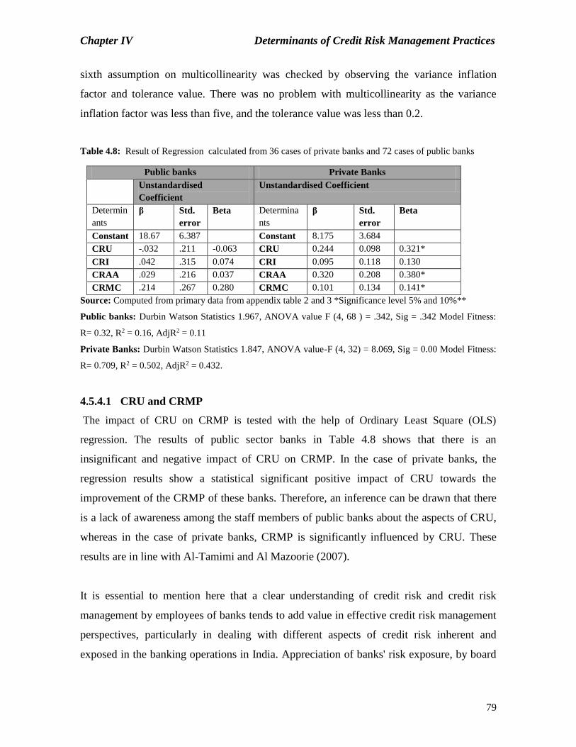
Chapter IV Determinants of Credit Risk Management Practices
79
sixth assumption on multicollinearity was checked by observing the variance inflation
factor and tolerance value. There was no problem with multicollinearity as the variance
inflation factor was less than five, and the tolerance value was less than 0.2.
Table 4.8: Result of Regression calculated from 36 cases of private banks and 72 cases of public banks
Public banks Private Banks
Unstandardised
Coefficient
Unstandardised Coefficient
Determin
ants
β Std.
error
Beta Determina
nts
β Std.
error
Beta
Constant 18.67 6.387 Constant 8.175 3.684
CRU -.032 .211 -0.063 CRU 0.244 0.098 0.321*
CRI .042 .315 0.074 CRI 0.095 0.118 0.130
CRAA .029 .216 0.037 CRAA 0.320 0.208 0.380*
CRMC .214 .267 0.280 CRMC 0.101 0.134 0.141*
Source: Computed from primary data from appendix table 2 and 3 *Significance level 5% and 10%**
Public banks: Durbin Watson Statistics 1.967, ANOVA value F (4, 68 ) = .342, Sig = .342 Model Fitness:
R= 0.32, R2 = 0.16, AdjR2 = 0.11
Private Banks: Durbin Watson Statistics 1.847, ANOVA value-F (4, 32) = 8.069, Sig = 0.00 Model Fitness:
R= 0.709, R2 = 0.502, AdjR2 = 0.432.
4.5.4.1 CRU and CRMP
The impact of CRU on CRMP is tested with the help of Ordinary Least Square (OLS)
regression. The results of public sector banks in Table 4.8 shows that there is an
insignificant and negative impact of CRU on CRMP. In the case of private banks, the
regression results show a statistical significant positive impact of CRU towards the
improvement of the CRMP of these banks. Therefore, an inference can be drawn that there
is a lack of awareness among the staff members of public banks about the aspects of CRU,
whereas in the case of private banks, CRMP is significantly influenced by CRU. These
results are in line with Al-Tamimi and Al Mazoorie (2007).
It is essential to mention here that a clear understanding of credit risk and credit risk
management by employees of banks tends to add value in effective credit risk management
perspectives, particularly in dealing with different aspects of credit risk inherent and
exposed in the banking operations in India. Appreciation of banks' risk exposure, by board

Chapter IV Determinants of Credit Risk Management Practices
80
members, executive management, and other employees are significant for effective risk
management (Hussain and Azmi, 2012). The result of a public and private bank does not
support the Institutional theory, because the theory claims that CRU among public and
private banks is uniform, however the results show that CRU has an insignificant impact on
CRMP in case of public banks, whereas CRU has a significant impact on CRMP in case of
private banks. This violates the assumption of the homogeneity of institutional theory. The
theory is not working concerning independent variable CRU on account of difference in the
common understanding among the employees on the different aspects of CRU followed by
public and private banks in India.
4.5.4.2 CRI and CRMP
The impact of CRI on CRMP of banks in India highlights that CRI has an insignificant
impact on CRMP. These findings are contradicting with the results of relevant studies such
as Al-Tamimi and Al-Mazrooei (2007), Hussain and Al-Ajmi (2012), Ishitiq (2015). The
results are contradicting because these studies are conducted in different countries having
different economic background. The studies by Al-Tamimi and Al-Mazrooei (2007) and
Hussain and Al-Ajmi (2012) are conducted in the UAE and Ishitiq (2015) study is
conducted in Pakistan. Furthermore, these findings do not support the policy implications
of the Reserve Bank of India (RBI) guidelines. The RBI’s guidelines in its notification
stated that top management of banks should attach considerable importance to improve the
ability to identify the overall level of risk undertaken. However, in practice these banks are
not procuring full information from borrowers before granting a loan to them. Therefore,
the NPA's of these banks have shown an increasing trend over some time. As per the RBI’s
report, a fact from Business Standard (2019), reveals that total NPA's of banks has
increased by more than 300% in ten years from 2006-07 to 2016-17. This could be on
account of improper CRI by banks.
4.5.4.3 CRAA and CRMP
The result of public sector banks shows that there is an insignificant impact of CRAA on
the CRMP. This result shows that there is a lack of credit risk analysis and assessment
process in public sector banks. However, the results of private banks in India show a

Chapter IV Determinants of Credit Risk Management Practices
81
significant positive impact of CRAA on the CRMP. Therefore, an inference can be drawn
that CRMP in the private banking industry is significantly influenced by CRAA. These
findings are also compliable with the results of Al-Tamimi and Al-Mazrooei (2007) and
Ishitiq (2015), indicating a significant relationship between CRAA and CRMP in case of
Indian private banks.
The private banks are applying their skills before granting a loan to the customer.
Therefore, the NPA's of private banks are less compared to public sector banks. As per
RBI’s report, a fact from Business Standard (2019) reveals that public sector bank's Gross
NPA to Gross Advance ratio was 2.8% in 2006-07 and reached 11.8% in 2016-17.
Similarly, private sector banks exhibit statistics of the same ratio as 2.2% in 2006-07 to
4.3% in 2016-17. Rosman (2009), in its study believes that CRAA, particularly on
measuring risk in a banking institution, is vital for CRMP. Therefore, public sector banks
are expected to make a CRAA policy for having an effective CRMP. As per the guidance
note of RBI, all the local banks must implement a system for risk assessment and analysis
to fulfill the regulatory requirement. Guidance note on credit risk management direct all the
banks to make compact approaches for the risk assessment and analysis in order to provide
a robust framework for risk management in these financial institutions. In total, the results
of the public and the private banks are paradoxical, hence the findings are contradicting the
uniformity assumption of Institutional Theory. The public and the private banks are not
following the uniform norms, rules, practices for managing credit risk, hence CRAA of
public and private banks differs.
4.5.4.4 CRMC and CRMP
The relationship between CRMC and CRMP of public and private banks in India is tested
and shown in Table 4.7. According to the results, the public sector banks show an
insignificant impact of CRMC on the CRMP. This result shows that there is a lack of credit
risk monitoring and control processes in public sector banks. The results of the present
study concerning public banks throw light on the partial compatibility of the guidance note
on CRAA given by RBI. Finally, the results of the present study shows that public sector
banks are not following proper procedures for CRMC to improve the CRMP of banks.

Chapter IV Determinants of Credit Risk Management Practices
82
However, private banks show a significant positive impact of CRMC on the CRMP of
banks in India. Based on these empirical facts, it indicates that CRMC is an essential
determinant of CRMP in the case of private banks in India. These findings are compatible
with the results of relevant studies Al-Tamimi and Al-Mazrooei (2007), Hussain and Al-
Azmi (2012) and Ishitiq (2015).
Overall the contribution of CRMC to CRMP differs concerning public and private banks as
per the results are shown in Table 4.7. The findings are contradicting to the homogeneity
assumption of Institutional Theory. Finally, RBI guidelines given in the guidance note
states that top management of banks should attach considerable importance to improve the
ability to identify the overall level of risk undertaken. Considering this fact, guidelines of
RBI it is expected that all the banking institutions are required to implement a
comprehensive and rigorous mechanism of risk monitoring and control in India to have an
effective CRMP.
The result of regression demonstrates that CRU, CRI, CRAA and CRMC were found to
have statistical insignificant influence on the CRMP of public banks. This result helps us to
accept the null hypothesis (H01). The influence of CRU, CRAA and CRMC were
significant on the CRMP of private banks, which fails to accept the null hypothesis (H01).
The regression results of private banks are in line with Al - Tamimi (2007), Rosman
(2009), Nazir et al. (2012) and Jorge Naghu (2017).
4.5.4.5 Model Fit
An OLS regression was run to understand the impact of CRU, CRI, CRAA and CRMC on
the CRMP of public and private banks. Table 4.8 shows the results of regression analysis
on public and private sector bank's data. The Results of public sector banks show that
adjusted R2 is 0.11, which means that 11% of the variation in the dependent variable that is
CRMP is due to the explanatory variables (CRU, CRI, CRAA, and CRMC) and remaining
89% variation is due to other factors. F value is not significant at 1%; hence, we can say
that the overall Model is not a good fit. The value of beta (β) explains the contribution of
the independent variable. CRMC shows the highest beta value, which means its
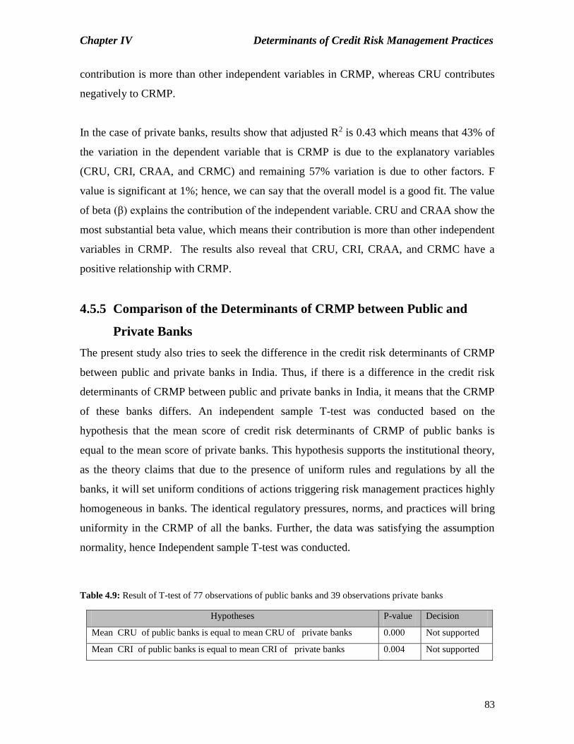
Chapter IV Determinants of Credit Risk Management Practices
83
contribution is more than other independent variables in CRMP, whereas CRU contributes
negatively to CRMP.
In the case of private banks, results show that adjusted R2 is 0.43 which means that 43% of
the variation in the dependent variable that is CRMP is due to the explanatory variables
(CRU, CRI, CRAA, and CRMC) and remaining 57% variation is due to other factors. F
value is significant at 1%; hence, we can say that the overall model is a good fit. The value
of beta (β) explains the contribution of the independent variable. CRU and CRAA show the
most substantial beta value, which means their contribution is more than other independent
variables in CRMP. The results also reveal that CRU, CRI, CRAA, and CRMC have a
positive relationship with CRMP.
4.5.5 Comparison of the Determinants of CRMP between Public and
Private Banks
The present study also tries to seek the difference in the credit risk determinants of CRMP
between public and private banks in India. Thus, if there is a difference in the credit risk
determinants of CRMP between public and private banks in India, it means that the CRMP
of these banks differs. An independent sample T-test was conducted based on the
hypothesis that the mean score of credit risk determinants of CRMP of public banks is
equal to the mean score of private banks. This hypothesis supports the institutional theory,
as the theory claims that due to the presence of uniform rules and regulations by all the
banks, it will set uniform conditions of actions triggering risk management practices highly
homogeneous in banks. The identical regulatory pressures, norms, and practices will bring
uniformity in the CRMP of all the banks. Further, the data was satisfying the assumption
normality, hence Independent sample T-test was conducted.
Table 4.9: Result of T-test of 77 observations of public banks and 39 observations private banks
Hypotheses P-value Decision
Mean CRU of public banks is equal to mean CRU of private banks 0.000 Not supported
Mean CRI of public banks is equal to mean CRI of private banks 0.004 Not supported

Chapter IV Determinants of Credit Risk Management Practices
84
Mean CRAA of public banks is equal to mean CRAA of private banks 0.000 Not supported
Mean CRMC of public banks is equal to mean CRMC of private banks 0.000 Not Supported
Source: Authors calculations from appendix table 4.3, Note: Significance level at 5%
The result of the independent sample t-test fails to accept the null hypothesis. The result
shows a significant difference in the credit risk determinants of CRMP of public and private
banks with respect to all the four determinants. This result is supported by the result of the
regression analysis present study. The result of the regression analysis of public and private
banks differs. The result of the Independent sample T-test is contradicting to the uniformity
assumption of Institutional theory, on the ground that, CRMP of public and private banks
differs as per the result of T-test and regression analysis. The difference in the result of
public and private banks may be on account of weak determinants of CRMP of public
sector banks as the mean of public sector banks is low compared to private banks. Thus,
public sector banks need improvement in determinants of CRMP such as CRU, CRI,
CRAA and CRMC.
4.6. Summary
The aim of this study was to investigate empirically the influence of credit risk
determinants on CRMP of the public and the private banks operating in India. To achieve
this objective, the credit risk determinants of CRMP were identified with the help of data
collection tool such as questionnaire and data analysis tool such as Principal Component
analysis. Based on the literature review, it was found that most of the studies in the past
have used five determinants and all types of risk under the Risk Management Practices
(RMP). The present study found four determinants using a rotated component matrix of
Principal component analysis as it has subsumed the additional variable into an existing
variable. These four determinants do not present a good fit for the model in the case of
public sector banks, hence there is a need to add some more statements and find more
determinants.
The results of the descriptive analysis show that the mean score of private banks is better
than public banks. It means that the process followed for credit risk management in terms
of CRU, CRI, CRAA, and CRMC is superior for the private banks compared to public
banks.

Chapter IV Determinants of Credit Risk Management Practices
85
In measuring the impact of the credit risk determinants on their respective CRMP for public
and private banks, regression results reveal that explanatory variable Credit Risk
Understanding and Credit Risk Assessment and Analysis (CRAA) among the four
components are most influential in the contribution of CRMP of private banks.
The result of regression demonstrates that credit risk determinants were found to have
statistical insignificant influence on the CRMP of public banks. This result helps us to
accept the null hypothesis (H01). However, the same determinants were significant on the
CRMP of private banks, which fails to accept the null hypothesis (H01). The regression
results of private banks are in line with Al - Tamimi (2007), Rosman (2009), Nazir et al.
(2012) and Jorge Naghu (2017). Thus, the regression model fits the data well for the private
banks compared to public banks in India and the results for private banks are consistent
with previous studies like that by Al-Tamimi and Al-Mazrooei (2007), and Hussain and Al-
Ajmi (2012).
Further, these regression results are also supported by the result of the independent sample
t-test. The results of the t-test show a significant difference in the credit risk determinants of
CRMP between public and private banks. These contradictory results between the public
and the private banks violate the assumption of uniformity of the Institutional theory.
Finally, the results of the present study provided empirical confirmations that private
banks are generally better in understanding the credit risk, using techniques for
identification of credit risk, following proper process for credit risk assessment and
analysis, and adopting the right approach for credit risk monitoring and control. This
indicates the ability of these banks to manage risks efficiently in the future.
Chapter V Measurement of Credit Risk Management Practices
86
Chapter V
Measurement of Credit Risk Management Practices
5.1 Introduction
The growing complexities of the bank’s business due to liberalization, deregulations,
technical up-gradation, and the dynamic operating environment, gave rise to credit risk.
Credit risk refers to the probability of counterparty failing to repay a debt to an
organization, arises due to lending activities. The credit risk is a curse for banks for
decades as it has a devastating effect in terms of financial loss to the banks. This demands
banks to deploy powerful CRMP, which aids in the measurement of credit risk.
Measurement of credit risk means quantification of risk from credit operations using
quantitative variables such as lending and financial ratios. Measurement of credit risk is an
essential mechanism for preventing financial losses and maintaining continuity of the
banking business. It provides a mechanism for monitoring credit risk and reliable reporting.
Today the banks are facing an increasing trend of Non-Performing Assets (NPAs)
triggering insight into credit risk measurement. Thus credit risk measurement perceives
higher significance due to the higher NPA level of Indian banks compared to the global
benchmark. As per the RBI report, the facts state that Gross NPA to Gross Advance ratio of
a public bank is 11.59 % (March 2019), as against it is 2.99% for foreign banks. For the last
few years, (NPAs) have emerged as an inevitable burden on the government and RBI.
Several steps have been undertaken by both to curb the increasing NPA of Indian banks,
but these steps proved to be unsuccessful. This situation drives the attention of the banker
towards understanding the financial position of its banks. Assessment of financial position
can serve the specific needs through reforms in financial data.
There are several ways to make reforms in the financial data of the banks, and one of the
conventional methods used is ratio analysis. Ratio analysis is a more sophisticated method
as it provides a more detailed explanation since it considers correlations between two
variables. Therefore, the present study used a credit risk related ratio analysis as a tool for

Chapter V Measurement of Credit Risk Management Practices
87
the measurement of credit risk. This tool helps in internal risk monitoring for banks. A
trend in specific ratios will help to draw generalizations about credit risk in public and
private banks.
In the present study, credit risk related ratios such as lending and financial ratios are used.
Lending ratios are loan related ratios, which convey data about asset quality and loan
account position of the banks. These ratios evaluate the position of the performing and
Non-performing assets, and the assessment of the loan account plays a vital role in meeting
the financial obligations of the business. This study measures credit risk using eight lending
ratios.
A measurement of CRMP with the aid of financial ratios assists in understanding financial
position in terms of liquidity, profitability, and leverage position of banks. The regulators
from time to time are in search of different methods to compare the financial position of
banks. Thus, measuring credit risk using financial ratios helps the bank regulators to
evaluate the comparative performance of banks. Data regarding the financial position of the
banks shows the effectiveness of CRMP adopted by banks. The present study measures
CRMP using liquidity, profitability, and leverage variable, with the assistance of financial
ratios. The reason for using these variables is, in subsequent chapter four models are used
to predict the bankruptcy of banks, and these four models used liquidity, leverage, and
profitability variable to predict the bankruptcy of banks. Therefore, financial ratios
measuring these variables are considered in the present study.
An analysis of profitability, liquidity, and leverage position, helps to understand the
financial position of banks as it is positively affected by these three variables, or one is
achieved at the cost of others. The liquidity, profitability, and leverage are found to be the
essential determinants for the success and survival of the banks; hence there should be an
optimum tradeoff between these three variables. Considering the above, the present study
finds the interrelationship between these three variables and measures CRMP using these
three variables. Thus study on correlation analysis will help the researcher to understand the
strength and the direction of the relationship. Further, the available literature states an
Chapter V Measurement of Credit Risk Management Practices
88
inverse relationship between liquidity and profitability and also between profitability and
leverage. An effort is made to judge the same concerning the Indian context.
These above issues drive the researcher to measure and compare the credit risk
management practices of public and private banks using lending ratio and financial ratio.
The banks need to divert their scarce resources towards the effective management of credit
risk based on the analysis of lending and financial ratios. A study on measuring and
comparing credit risk will help to understand the asset quality position of a bank. Similarly,
a study of financial ratios will help to analyze the trend in liquidity, profitability, and
leverage variables with the help of time-series and cross-sectional data.
The present chapter is an empirical chapter that summarizes the findings from the
secondary data. This chapter consists of results and discussion into three parts. Part I
explains the measurement and comparison of CRMP using the lending ratio of public and
private banks in India. Part II comprises of measurement and comparison of liquidity,
profitability, and leverage position the banks using financial ratios. Part III covers the
identification of the relationship between liquidity, profitability, and leverage.
5.2 Literature Review
The recent history of financial crisis 2008 induced financial analysts to develop literature
on the CRMP. It is found from the literature that the ratios for measurement of credit risk
differ from bank to bank, although all the banks face the same extent of credit risk. A study
by Thiagarajan (2011) found a significant difference between public and private banks
concerning specific key ratios. A study of Kattel (2016), found a significant difference in
the mean value of credit risk ratios of private and joint-venture banks in Nepal using a tool
one way ANOVA. A study by Kumar and Pourkiaei (2016) shows a significant difference
between public, private, and foreign banks with regards to specific ratios. A study by Rekhi
and Goel (2013) compared the performance of public and private banks, conclude that new
banks are more efficient than old ones.
The liquidity, profitability, and leverage are important determinants for the success and
survival of the bank. There should be an optimum tradeoff between all these three
variables. Some of the past studies developed a relationship between liquidity and

Chapter V Measurement of Credit Risk Management Practices
89
profitability in the case of the banking industry. These studies are Lartey et al. (2013),
Abdullah (2014), Malik and Khursheed (2016), Awais (2016), Nabeel and Hussain (2017),
and Sharma (2017).
Some studies in the past found a weak and insignificant relationship between profitability
and liquidity. A study by Lartey et al. (2013), found a weak relationship between liquidity
and profitability of the banks listed on the Ghana stock exchange. Similarly, a study by
Malik and Khursheed (2016) found e negative relationship profitability and liquidity. Also,
a study by Nabeel and Hussain (2017) concludes that cash and current ratios show negative
relations, whereas quick ratio and CAR show positive relations towards profitability.
Abdullah (2014) concludes that there is no significant relationship between liquidity and
profitability. However, a study by Awais (2016) found a significant relationship between
the liquidity and profitability of banks in Pakistan whereas, a study by Ahmed (2016)
reveals that there is a positive as well as an inverse relationship between profitability and
liquidity.
The leverage ratio measures the extent to which a bank has financial assets with equity.
Some of the studies found a positive relationship between profitability and leverage
variable. However, some other studies conclude the inverse relationship between
profitability and leverage. A study by Zafar and Fartyal (2015) concludes that leverage has
an inverse impact on the profitability of the banks. A study by Ebiringa (2012) found a
negative effect of leverage on the performance of the bank. A study by Taani (2013)
concludes that the presence of high leverage affects the return on banks. However,
Moghaddam (2017) study concludes that there is a significant positive effect of liquidity
and leverage on the earnings of the firm. Thus most of the studies claim a negative
relationship between leverage and profitability.
Literature in the area of understanding the relationship between liquidity and leverage is
less, as also the liquidity and its effect on the debt level have been a controversial issue
among scholars in finance studies. Prior studies have demonstrated that liquidity increased
debt level while other studies found that high liquidity was less leveraged and more
regularly financed by their capital. A study by Ghasemi and Rajak (2016) concludes that a
quick ratio has a positive effect on leverage, whereas the current ratio harms the leverage.

Chapter V Measurement of Credit Risk Management Practices
90
There is a difference in the profitability, liquidity, and leverage position of public and
private banks in India. Thakarshibai (2014) concludes that there is an improvement in the
profitability of private banks compared to public banks. Balaji and Kumar (2016) study
concluded that the growth rate is higher for private banks, whereas public banks are lagging
in many financial parameters and are facing many challenges too. A study by Chintala
(2016), found that profitability is higher for private banks. Also, Katti and Vadrale (2018)
study concluded that the profitability position of the private bank is better than public
banks. A study by Khan (2018) and Koley (2019) concludes that the performance of private
banks is better as compared to public banks. Similarly, a study by Sharma (2017) found a
difference in the profitability of public and private banks. Patel and Bhanushali (2017)
study concluded that both sectors are profitable, and profitability is the greatest challenge
for banks. This literature shows that most of the studies focused on the profitability aspect
as a base for comparison between public and private banks. However, studies on banks'
liquidity and leverage as a base for comparison in the Indian context are very few.
5.3 Data and Methods
The present study is conducted to measure and compare the CRMP of public and private
banks in India using lending and financial ratio. In this study, the required data have been
sourced from audited statements of individual banks and RBI. Part of data is collected from
reputed data sources such as Centre for Monitoring Indian Economy (CMIE) and Indian
stats.com. The data was taken for thirteen years period from the year 2004-05 to 2016-17.
A total of 39 commercial banks (21 one Public banks and 18 private banks) were chosen as
sample based on the availability of data and the consequences of time limitations.
The ratio analysis technique is used to measure credit risk in select public and private banks
in India. Ratio analysis is the most powerful tool of financial analysis, and it is relevant in
assessing the performance in respect of liquidity position, operating efficiency, asset
quality, etc. In the present study, eight lending ratios are used to measure the credit risk of
public and private banks. These ratios are Gross NPA to Gross Advance Ratio, Net NPA to
Net Advance ratio, Total loan to Total Asset, Total loan to Total Deposit, Total Loan to
Total Equity, Provision for NPA to NPA, Capital Adequacy Ratio (CAR) and Return on
Asset (ROA). This study compares lending ratios between public and private banks using a

Chapter V Measurement of Credit Risk Management Practices
91
parametric test such as an Independent samples t-test. The assumptions required to run the
independent sample T-test, such as normal distributions and homogeneity of variance were
checked. The sample data is consistent with these assumptions.
The standard One Way ANOVA test was conducted to test the difference is statistically
significant amongst the 21 public banks group and 18 private banks group. The
assumptions required to run ANOVA, such as continuous dependent variable,
independence of observation, normal distribution, and homogeneity of variance were
checked before the application of ANOVA. The sample data were made in line with these
assumptions. Further, a post hoc test was conducted to find, the bank which contributes to a
statistically significant difference in the group.
This study also used ‘Financial Ratios’ to measure the liquidity, profitability, and leverage
position of the public and private banks in India. In this study, nine financial ratios are used
to measure the above variables. These ratios are taken from the bankruptcy model used in
the further part of the present study. For the sake of simplicity, codes are given to financial
ratios, which are mentioned in the following table.
Table 5.1: Codes to Financial Ratios used by Bankruptcy Models
Liquidity Profitability Leverage
Financial Ratio Bankruptcy
Model
Financial Ratio Bankruptcy Model Financial Ratio Bankruptcy Model
L1- Working
Capital to Total
Asset (WC/TA)
Altman Z-score
Springate Model
Grover Model
P1 – Earnings
Before Interest and
Tax/Total Asset
(EBIT/TA)
Altman Z-score
Springate Model
Grover Model
LV1-Retained
Earnings/Total
Asset (RE/TA)
Altman Z-score
L2 - Current Asset/
Current liability
(CA/CL)
Zmijewski model P2 – Return on
Asset (ROA)
Grover Model
Zmijewski model
LV2-Market Value
of Equity /Total
Liability (MVE/TL)
Altman Z-score
P3 –Profit Before
Interest and
Tax/Current
Liability
(PBIT/CL)
Springate Model
LV3 – Total
Deposit /Total
Asset (TD/TA)
Zmijewski model
P4- Total Income
(TI)/Total Asset
(TA)
Springate Model
Source: Authors compilations

Chapter V Measurement of Credit Risk Management Practices
92
Table 5.1 shows that the variable Liquidity is measured using Working Capital to Total
Asset (L1), and Current Asset to Current Liabilities (L2). The variable Profitability is
measured using Earnings before Interest and Tax to Total Assets (P1), Return on Asset
(P2), Earnings Before Interest and Tax to Current Liability (P3), and Total Income to Total
Asset (P4). While the Leverage is measured using Retained Earnings to Total Asset (LV1),
Market Value of Equity to Total Liability (LV2), and Total Deposit to Total Asset(LV3).
Table 5.1 shows that ratio L1 and P1 is used by most of the bankruptcy model.
Time-series data for a period from 2004-05 to 2016-17 and cross-sectional data of 21 public
sector banks and 18 private banks was used to compare the liquidity, profitability, and
leverage position of public and private banks in India. The parametric test, such as the
Independent sample t-test, was used for normal data, and the non-parametric test such as
Mann Whitney U-test was used for non-normal data. This test will help the researcher to
generalize and compare the liquidity, profitability, and leverage position of public and
private banks in India. Further, Pearson’s correlation coefficient is used to find the
correlation between liquidity and profitability, profitability and leverage, liquidity, and
leverage that will state the existence, direction, and strength of the relationship.
5.4 Result and Discussion
This chapter consists of results and discussion into three parts. Part I comprises
measurement and comparison of CRMP using lending ratios. Part II comprises of
measurement and comparison of CRMP using financial ratios, and part III consists of
identification of the relationship between the financial variables such as liquidity,
profitability, and leverage.
5.4.1. Measurement and Comparison of CRMP using the Lending Ratios
This part measures and compares the CRMP using eight lending ratios such as Gross NPA
to Gross Advance Ratio, Net NPA to Net Advance ratio, Total loan to Total Asset, Total
loan to Total Deposit, Total loan to Total Equity, Provision for NPA to NPA, CAR, and
ROA. Independent sample T-test and ANOVA is used to test the following null hypothesis.
H01: There is no statistical difference in the lending ratios between and amongst the public
and private banks in India.
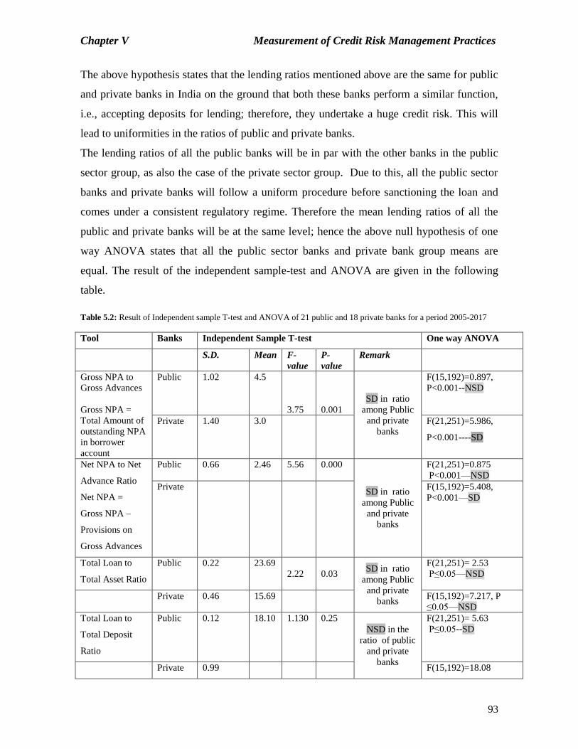
Chapter V Measurement of Credit Risk Management Practices
93
The above hypothesis states that the lending ratios mentioned above are the same for public
and private banks in India on the ground that both these banks perform a similar function,
i.e., accepting deposits for lending; therefore, they undertake a huge credit risk. This will
lead to uniformities in the ratios of public and private banks.
The lending ratios of all the public banks will be in par with the other banks in the public
sector group, as also the case of the private sector group. Due to this, all the public sector
banks and private banks will follow a uniform procedure before sanctioning the loan and
comes under a consistent regulatory regime. Therefore the mean lending ratios of all the
public and private banks will be at the same level; hence the above null hypothesis of one
way ANOVA states that all the public sector banks and private bank group means are
equal. The result of the independent sample-test and ANOVA are given in the following
table.
Table 5.2: Result of Independent sample T-test and ANOVA of 21 public and 18 private banks for a period 2005-2017
Tool Banks Independent Sample T-test One way ANOVA
S.D. Mean F-
value
P-
value
Remark
Gross NPA to
Gross Advances
Gross NPA =
Total Amount of
outstanding NPA
in borrower
account
Public 1.02 4.5
3.75
0.001
SD in ratio
among Public
and private
banks
F(15,192)=0.897,
P<0.001--NSD
Private 1.40 3.0 F(21,251)=5.986,
P<0.001----SD
Net NPA to Net
Advance Ratio
Net NPA =
Gross NPA –
Provisions on
Gross Advances
Public 0.66 2.46 5.56 0.000
SD in ratio
among Public
and private
banks
F(21,251)=0.875
P<0.001—NSD
Private F(15,192)=5.408,
P<0.001—SD
Total Loan to
Total Asset Ratio
Public 0.22 23.69
2.22
0.03 SD in ratio
among Public
and private
banks
F(21,251)= 2.53
P≤0.05—NSD
Private 0.46 15.69 F(15,192)=7.217, P
≤0.05—NSD
Total Loan to
Total Deposit
Ratio
Public 0.12 18.10 1.130 0.25
NSD in the
ratio of public
and private
banks
F(21,251)= 5.63
P≤0.05--SD
Private 0.99 F(15,192)=18.08

Chapter V Measurement of Credit Risk Management Practices
94
≤0.05--SD
Total Loan to
Total Equity
Ratio
Public 269 288 -1.2 0.2
NSD in a ratio
of Public and
private banks
F(21,251)= 27.43
P≤0.05--SD
Private 160 193 F(15,192)=18.90, P
≤0.05--SD
Provision to
NPA to NPA
ratio
Public 0.70 16.81 -1.8 0.06
SD in a ratio
of Public and
private banks
F(21,251)= 44.77
P≤0.05--SD
Private 0.5 F(15,192)=6.088, P
≤0.05--SD
Return on Asset Public .22 15.60
-2.60
0.009 SD in a ratio
of Public and
private banks
F(21,251)= 2.368,
P≤0.05--SD
Private .98 25.1 F(15,192)= 2.20 P
≤0.05--SD
Capital
Adequacy Ratio
Public 0.74 15.7 -2.60 0.009
SD in the ratio
of public and
private banks
F(21,251)= 4.144,
P≤0.05--SD
Private 4.3 25 F(15,192)= 7.53 P
≤0.05--SD Notes: Significant Difference (SD), Non-Significant Difference (NSD), Source: Authors Calculation using data from appendix table A.4
to A.21
5.4.1.1 Gross NPA to Gross Advance ratio
Gross NPAs comprises of all the non-standard assets like as sub-standard, doubtful, and
loss assets. The Gross NPA consists of (Balance in Interest Suspense account+ Claims
received from Deposit Insurance Credit Guarantee Corporation Export Credit Guarantee
Corporation and pending for adjustment + Part-payment received and kept in suspense
account + Total provisions held). The lower the ratio is, the better it is. The gross NPA is
always shown as a percentage of advances.
A time-series data presented in annexure table A.4 and A.5 shows all the public banks in
the decreasing trend of this ratio from the year 2005 to 2012. The ratio has gradually
increased from 2013 to 2017. This increase may be due to improper CRMP resulting in a
higher ratio. Similarly, all the private banks also show the decreasing trend of this ratio
from the year 2005 to 2013, and it shows a gradual increase in the ratio from 2014 to 2017.
This rise could be on account of an increase in the ratio of Catholic Syrian banks, City
Union Bank, ICICI Bank, and Nainital bank, as these banks ratio shows an increasing trend
continuously for a period of four years (2014 – 2017).
There is a statistically significant difference in the Gross NPA to the Gross Advance ratio
in the group of private banks as per table 5.2. A post hoc test result shows the statistical

Chapter V Measurement of Credit Risk Management Practices
95
difference lies in the Yes bank in the private bank group. However, One Way-ANOVA
result for public sector banks shows that there was no statistical difference in the mean
Gross NPA to Gross Advance ratio between different banks in the public sector group.
The annexure table A.4 and A.5 shows the gross NPA to gross advance ratio of 13% and
4% for public and private banks respectively in the latest years. This trend shows a
difference in this ratio between public and private banks, supported by the results of the
Independent sample T-test (Table 5.2), and this difference depicts a difference in the
CRMP of public and private banks.
5.4.1.2 Net NPA to Net Advance ratio
The Net NPA’s are calculated by deducting provisions from Gross NPA. Lower the ratio
better it is for the bank’s prosperity. Time series data presented in annexure table A.6
shows a decreasing trend in this ratio for public sector banks from 2005-2009; however, it
started rising from 2010-2017. The private banks, however, showed a fluctuating trend in
this ratio over thirteen years and was consistently low for these banks, as per annexure table
A.7. This shows the difference in the trend of public and private banks, and also, this ratio
is high for public banks. The average ratio reached 8.10 and 2.69 for public and private
banks, respectively, in the year 2017. All these facts reveal a difference in this ratio of
public and private banks supported by the results of the Independent sample t-test in table
5.2.
The result of one Way-ANOVA shows no statistically significant difference in this ratio
amongst different banks in the public sector group. However, private banks show a
significant difference amongst different banks. A post hoc test result shows the statistical
difference lies in the Catholic Syrian Bank and Yes Bank in the private bank group, as also
the ratio was highest for Catholic Syrian bank and lowest for the Yes bank as per annexed
Table A.7.
5.4.1.3 Total Loan to Total Asset Ratio
Loan to Asset ratio measures the total loan outstanding as a percentage of total assets.
Banks that have a relatively higher loan to asset ratio derive more of their income from loan
and investment.

Chapter V Measurement of Credit Risk Management Practices
96
Time series data presented in annexure A.8 and A.9 showed an increasing trend from 2005
to 2017 in the case of public and private banks, as both the sectors have crossed the ratio
over 0.5. This ratio 0.5 indicates that the loan sanctioned by the banks is more than half of
the assets present with the bank. This depicts, banks have increased their lending business
over some time, maybe to face fierce competition with each other and with the foreign
players.
The one way-ANOVA result shows a statistically significant difference amongst the
different banks in the public sector group. The post hoc test shows a statistical difference
lies due to the mean ratio of Syndicate and the United Bank of India. There was also a
statistically significant difference in the Total loan to Total Asset ratio of private banks. A
post hoc test result shows the statistical difference lies in the City Union Bank in the private
bank group.
The variance in the mean ratio among public banks is low, whereas among private banks is
high. This shows a difference in the ratio of public and private banks supported by the
results of the Independent sample t-test in table 5.2.
5.4.1.4 Total Loan to Total Deposit Ratio
This ratio helps to assess the liquidity and aggressiveness of bank management. This ratio
specifies how much a bank lends out of deposits it has mobilized. A higher the ratio
indicates, riskier a bank may be at higher defaults and more dependent on deposits for
lending and vice versa. A meager ratio indicates banks are not making full utilization of
their resources, and if the ratio is above a certain level, it indicates pressure on the
resources.
A time-series data presented in annexure A.10 and A.11 shows an increasing trend in this
ratio throughout 2005-2017. This signifies that banks have increased their loan business for
over thirteen years. The pattern of increasing trend also shows no difference in this ratio
between public and private banks. As a shred of evidence for the same, are the results of the
Independent sample t-test in table 5.2, which indicates that there is no statistically
significant difference in this ratio between public and private banks.
The one way ANOVA table shows a statistically significant difference amongst different
banks in the public sector group and private banks group. A post hoc test reveals the

Chapter V Measurement of Credit Risk Management Practices
97
difference lies due to the mean ratio of IDBI and ICICI banks from public and private
groups, respectively.
5.4.1.5 Total Loan to Total Equity Ratio
This ratio expresses the relationship between total loan outstanding and the total equity of
the bank. This ratio helps the investor to analyze the equity position of the bank to make an
investment decision. It also explains the extent to which shareholders' equity can fulfill the
loan obligations of banks. Lower the ratio better it is for the stakeholders.
Time series data presented in annexure A.11 and A.12 show an increasing trend over
thirteen years from 2005-2017. An increasing trend signifies that banks have expanded
their lending business. This hike could be on account of policies of RBI or may be due to
market factors such as the entry of new players. The trend also shows no difference in this
ratio of public and private banks, supported by the results of the Independent sample t-test
in table 5.2.
There was a statistically significant difference in this ratio amongst the different banks in
public and private sector groups as per one way ANOVA table. A post hoc test reveals a
statistical difference lies due to the difference in the ratio of State Bank of India and Bank
of Maharashtra in the public sector group and HDFC and DCB in private bank group.
Overall Total loan to total equity ratio shows that all the banks from the sample have high
loans outstanding compared to its equity capital. This shows that banks have financed its
loan through deposits and other borrowed funds. Although this strategy is favorable to
equity holders in terms of getting the benefit of "Trading on Equity", however, it may
endanger the bank’s financial position if the loan turns into NPA. Thus banks in a sample
have expanded their lending business at the cost of equity, which may endanger the
financial position of the banks in the long term due to financial instability.
5.4.1.6 Provision for NPA to NPA ratio
This ratio highlights the extent of provisioning done on the existing NPA, thereby
indicating future provisioning requirements in the event of no recovery from the stock of
NPA. It indicates the degree of safety measures adopted by banks and has a direct bearing
on the profitability, dividend, and safety of shareholders. Higher the ratio better it is for the
banks from a safety point.

Chapter V Measurement of Credit Risk Management Practices
98
Time series data presented in the annexed table A.14 shows a public sector banks had a
decreasing trend for the last thirteen years except for the year 2013. On an average
provision, this ratio is low private banks, and the trend of this ratio differs among public
and private banks, this fact is supported by the results of the Independent sample t-test in
table 5.2.
The One way ANOVA table shows a statistically significant difference in the mean of this
ratio amongst the banks from the private group and the banks from the public sector group.
A post hoc test was conducted to find which bank reveals a statistical difference. The test
result shows the statistical difference lies in the Nainital and Laxmi Vials bank in the
private bank group and Union Bank of India and State Bank of India from the public sector
group.
5.4.1.7 Return on Asset (ROA)
It is the profitability ratio measured in terms of the relationship between net profit and total
assets. The ROA is frequently applied to banks because cash flow analysis is more
challenging to construct accurately.
This ratio for public sector banks showed minor fluctuations in the trend from 2005-2013;
however, it has decreased drastically in the year 2014 to 2017. This may be due to negative
returns of the United Bank of India and Indian Overseas Bank, Corporation Bank, Dena,
IDBI, and Central bank of India. One way-ANOVA table shows that there was a
statistically significant difference in the mean ROA ratio of different banks in the public
sector group. A post hoc test result shows a statistical difference lies due to the mean ratio
of Indian banks and the Central bank of India. The ‘ROA’ of the private bank has increased
over some time. One way ANOVA table shows a statistically significant difference in the
ROA of these banks. A post hoc test result reveals that the difference is on account of
Kotak Mahindra Bank, HDFC, Catholic Syrian bank, in the private bank group. During the
year 2017, the ‘ROA’ of private banks is almost 200% higher than public banks.
Overall, ‘ROA’ of a private bank is better than public sector banks, indicating a better
profitability position and credit risk management strategy of private banks. This difference
is supported by the results of the Independent Sample t-test in table 5.2.

Chapter V Measurement of Credit Risk Management Practices
99
5.4.1.8 Capital Adequacy Ratio (CAR)
It is a ratio that measures the amount of bank capital expressed as a percentage of its risk-
weighted credit exposure. ‘CAR’ is precautionary ratio banks need to maintain to face their
NPA's The Basel III norms stipulated a capital to risk-weighted assets of 8%. However, as
per RBI norms, Indian scheduled commercial banks are required to maintain a CAR of 9%
while Indian public sector banks are emphasized to maintain a ‘CAR’ of 12%. The
annexed table A.18 and A.19 show all the public and private banks have consistently
maintained the CRAR norm of 8% as prescribed by BCBS and 9% prescribed by RBI. This
shows the precautionary role played by all banks to avoid financial distress.
Overall, the private sector banks ‘CAR’ is better than Public banks. This shows the
difference in the ‘CAR’ of public and private banks. This difference is statistically
supported by the results of the Independent sample t-test. One way-ANOVA table shows
the statistically significant difference in the ‘CAR’ ratio amongst the different banks in the
public sector group and private sector group. Further, a post hoc test reveals a statistical
difference in the public sector group is due to the ratio of Bank of Baroda and private sector
group is due to Yes Bank, Catholic Syrian Bank, and the Karur Vysa Bank.
The overall results reveal a statistically significant difference in the majority of lending
ratios selected, and this result fails to accept the null hypothesis. In other words, it means
that there is a significant difference in the extent of credit risk between public and private
banks. The extent of credit risk is less in private banks may be due to low and manageable
NPAs with these banks.
These above findings state that public sector banks are facing unfavorable scenarios of
these lending ratios compared to private banks. These findings are in line with Velling
(2010), Thiagarajan et al. (2011), and Kattel (2016).
5.4.2. Measurement and comparison of CRMP using Financial Ratios
The financial ratios are used to analyze the liquidity, profitability, and leverage position of
the banks. Liquidity explains the availability of cash for immediate use at any point in time.
Profitability explains the degree to which the bank yields financial gain, and the leverage
variable measures the bank’s vulnerability to downturns. The measurement of these
variables is done with the help of a financial ratio. Liquidity is analyzed using two financial

Chapter V Measurement of Credit Risk Management Practices
100
ratios; Profitability is analysed using four financial ratios, and leverage is analysed using
three financial ratios. This analysis is carried with the help of the following hypothesis.
H02: There is no statistical difference in the financial ratio (liquidity, profitability, and
leverage) between the public and private banks in India.
The difference in these variables may not arise because both the banks belong to the same
industry and performing similar functions, and comes under the uniform regulatory regime
of RBI. Therefore there may not be a difference in the financial ratios between public and
private banks.
5.4.2.1 Liquidity Analysis
Liquidity at banks is a measure of its ability to readily find the cash to meet the demand
upon it. The banks need to maintain adequate liquidity levels as low safety margins may
endanger the bank's financial position. Basel III regulations stipulated 3% as the LCR.
Before these regulations, the Indian banking sector was lacking the regulations on
quantitative minimum regulatory requirements. In the present study, liquidity is measured
using ‘WC/TA (L1)’ and the Current Ratio (L2). The bankruptcy model applied in the
present study, such as Altman Z-score, Springate model, and Grover model used L1 while
the Zmijewski model, used L2 as a proxy to liquidity variable.
Table 5.3: Result of Independent sample T-test for liquidity analysis of time series data from year 2005-
2017and cross-sectional data of 21 public and 18 private banks
Proxy to variable Time Series
data
Mean
Results of Independent
Sample T-test/Mann-
Whitney U-test
Cross
Sectional Data
(Mean)
Results of
Independent
Sample T-test
Public WC/TA
(L1)
0.087 T(24 ) = -117,P=0.908
(NSD)
0.089 T(37 ) = -0.028,
P=0.978 (NSD) Private 0.088 0.089
Public CR (L2)- 3.912 T(24 ) = -0.128, P=0.898
(NSD) Mann Whitney U-
test
3.91 T(37 ) = -0.345,
P=0.732 (NSD)
Mann Whitney U-test
Private 3.754 3.75
Source: Authors calculations based on Appendix table from A.22-A.25, Notes Significant Difference (SD), Non-
Significant Difference (NSD),

Chapter V Measurement of Credit Risk Management Practices
101
The ‘WC/TA’ ratio is used as a measure to indicate the liquidity, and the current ratio
measures the banks short term solvency. The higher the ratio, the more is the bank's ability
to meet current obligations and higher is the safety for the funds of creditors.
Conventionally, a current ratio of 2:1 is considered satisfactory. The current ratio of public
as well as private banks is better as both these sectors have crossed the standard ratio 2:1 as
per annexed table A.24.
Time series data on ‘WC/TA’ ratio presented in annexure A.22 for public banks showed a
lower value of this ratio in the year 2005 and was negative for private banks in the same
year. This shows the poor liquidity position of private banks fifteen years back. Up to the
year 2009, ‘WC/TA’ of both sectors of banks was improving; however, it decreased in the
year 2010 by almost 22% and 23% in the case of public and private banks, respectively.
Since both the sectors ‘WC/TA’ ratio was low in the year 2010, it may be due to the impact
of macroeconomic factors. According to Elliott (2014), a bank’s liquidity situations,
particularly in a crisis, will be affected much more than just these reserves of cash and
highly liquid securities. Time series data relating to the current ratio annexed in table A.24
shows an increasing trend over thirteen years for public sector banks, whereas private banks
depict minor fluctuations.
Due to such a weak liquidity position of banks, Basel III norms introduced a type of buffer
known as Liquidity Coverage Ratio (LCR) to cover unexpected cash flows. Overall the
liquidity positions of both categories of banks show an improving trend for the last fifteen
years. This shows a similarity in the trend of the liquidity position of public and private
banks, supported by the results of independent sample t-test result in table 5.3.
The cross-sectional data on descriptive statistics presented in the annexure A.23 and A.25
shows that Bank of Baroda and Nainital bank has the highest mean ratio as well as obtained
maximum value from public and private category respectively, depicting the best liquidity
position of these banks. This fact is supported by the results of the Altman Z- score and
recalibrated Altman model, which shows the highest score for Bank of Baroda and Nainital
bank. The mean and minimum ‘WC/TA’ ratio was low for IDBI bank (public sector banks)
and Kotak Mahindra Ltd. (a private bank) during the last fifteen years. This depicts the
weak liquidity position of these banks supported by the results of Altman Z-score, which

Chapter V Measurement of Credit Risk Management Practices
102
shows IDBI in the distress position, maybe due to liquidity factor. The average mean
current ratio was maximum in the year 2017 for public banks and 2015 for private banks.
This is the post-implementation period of Basel III, whereby due to stringent rules and
regulations on liquidity coverage ratio by Basel III, all the banks may have improved its
liquidity position.
Finally, both these ratios showed the same results. Using both the ratios, Bank of Baroda
and Nainital bank from the public and private category show a better liquidity position.
Similarly, IDBI and Kotak Mahindra bank from the public and private category depict a
poor liquidity position. This fact is supported by the results of the Independent sample T-
test. These results help to accept the null hypothesis. Thus the liquidity position of both
public and private banks reflects the same situation.
5.4.2.2 Profitability Analysis
In the present study, profitability is measured using first ratio, ‘EBIT/TA’ ratio (P1), which
explains the amount of pre-interest and tax profit available to discharge short term
obligations. The second ratio, Return on Asset (P2), explains the ability of the company to
use its assets to create its profit. The third ratio ‘PBIT to CL (P3)’ explains the amount of
pre-interest and tax profit available to discharge short term obligations and the fourth one
‘TI/TA (P4)’ indicates that a high ratio is a good indicator. However, a too high ratio is not
necessarily a good indicator as it may be at the cost of high-risk loans subject to default.
The Altman Z-score model used P1, the Springate model used P1, P2, and P3, the Grover
model used P1 and P2, whereas the Zmijewski model used P2 as a proxy to profitability
variable in their respective models.
Table 5.4: Result of Independent sample T-test for profitability analysis of time series data from year 2005-
2017and cross-sectional data for 21 public and 18 private banks
Proxy to
variable
Time Series data
Mean
Results of
Independent Sample
T-test/ Mann Whitney
U-test
Cross
Sectional Data
(Mean)
Results of Independent
Sample T-test/ Mann
Whitney U-test
EBIT/TA-
Public
0.071 T(24 ) = 2.275, P = 0.084
(SD)
Mann Whiteny U-test
0.077 T(37 ) = -1.6, P = 0.0105
(SD)
Mann Whiteny U test

Chapter V Measurement of Credit Risk Management Practices
103
Private 0.072 0.079
ROA 0.666 T(24 ) = -1.9, P = 0.044
(SD)
Mann Whiteny U-test
0.667 T(37 ) = -2.5, P = 0.010
(SD)
Mann Whitney U-test
0.856 0.855
PBIT/CL 2.21 T(24 ) = -0.521, P =0.607
(NSD)
2.21 T(37 ) = -0.929, P = 0.359
(NSD)
2.05 2.5
TI/TA 0.085 T(24 ) = -3.01, P = 0.006
(SD)
0.084 T(37 ) = -4.4, P = 0.00
(SD)
0.093 0.092
Source: Authors calculations based on appendix table A.26-A.33. Notes Significant Difference (SD), Non-Significant
Difference (NSD).
Table 5.4 shows, majority of the profitability ratios reveals a significant difference in the
profitability ratios of public and private banks. These results fail to accept the null
hypothesis. This difference is supported by the fact that time-series data from the year
2005-2017 of annexure A.26, shows an increasing trend of ‘EBIT/ TA’ ratio of a public
sector bank. In contrast, in the case of private banks, it shows fluctuations. This ratio of
public and private banks was high in the year 2014 and low in the year 2005. Similarly, as
per annexure A.28, ‘ROA’ of public banks shows a decreasing trend from 2005-2017
signaling banks to improve their performance, whereas, in the case of private banks, it
shows fluctuations. During 2017 the ROA of a private bank was almost 200% higher than
public banks. Overall the ‘ROA’ of a private bank is better than public sector banks,
indicating a better profitability position and credit risk management strategy of this bank.
The ‘ROA’ of public banks has worsened over thirteen years, may due to increasing NPA.
The ratio of TI/TA ratio also supports the difference in the profitability position of public
and private banks. This ratio is consistently low for public banks in comparison to private
banks from 2005-2017.
The time-series data on ‘PBIT/CL’ ratio shows minor fluctuations and an increasing trend
from 2005-2017 for public and private banks. The mean ratio was lowest for both the
sectors in the year 2008. This may be on account of the marginal effect of the financial
crisis of 2008. This fact shows no difference in this ratio between public and private banks,
supported by the results of Independent sample t-test in table 5.4

Chapter V Measurement of Credit Risk Management Practices
104
The cross-sectional data on profitability ratios is presented in annexed table A.27, A.29,
A.31, and A.33. The cross-sectional data on ‘EBIT/TA’ shows Corporation bank (public
Bank) and City Union banks (private sector) show the highest mean ‘EBIT/TA’ ratio.
Similarly, the lowest mean ‘EBIT/TA’ ratio was for IDBI and Yes bank from public and
private banks, respectively. The cross-sectional data on ‘ROA’ shows Indian bank and
HDFC has the highest ‘ROA’ in case public banks and private banks, respectively. The
cross-sectional data on ‘PBIT/CL shows the highest values for Punjab and Sind Bank and
lowest for SBI. Similarly, in the case of the private category, it was highest for Karnataka
Bank Ltd and the lowest for HDFC. The minimum ratio of all the banks is below 1 in the
thirteen years of data period, and this signifies the insufficiency of profit to meet short term
obligations. The cross-sectional data on Total Income to Total Asset is highest for Indian
Bank and Kotak Mahindra bank among the public and private banks, respectively.
The trends in time series data cross-sectional data and the results of the t-test show a
significant difference in the profitability aspects of public and private banks in India. These
results are supported by the studies of Thakarshibai (2014), Balaji and Kumar (2016), Katti
and Vadrale (2018), Khan (2018), Koley (2019).
5.4.2.3 Leverage Analysis
The leverage variable measures the bank’s vulnerability to downturns. In the present study,
leverage is measured using ‘RE/TA (LV1)’, which indicates the ability of the firm to earn
profit and thereby securing retained earnings. The second leverage ratio ‘MVE/TL (LV2)’,
indicates the proportion of owners fund to the long term debt. A high value of ratio depicts
a firm's aggressiveness in financing its growth with debt. This rate shows the amount by
which the value of the assets of the firm can fall before the liabilities surmount the assets,
and thus the firm is insolvent. The third leverage ratio ‘TD/TA (LV3)’ measures the
relationship between total deposit and total asset.
Altman Z-score model used LV1 and LV2 as a proxy to leverage variable, and the
Zmijewski model used LV3 as a proxy to leverage variable in its models.

Chapter V Measurement of Credit Risk Management Practices
105
Table 5.5: Result of Independent sample T-test for leverage analysis of time series data from year 2005-
2017and cross-sectional data for 21 public and 18 private banks.
Proxy to
variable
Time Series data
Mean
Results of
Independent Sample
T-test
Cross
Sectional Data
(Mean)
Results of Independent
Sample T-test
RE/TA
Public
0.049 T(24 ) = -4.4, P=0.000
(SD)
Mann Whiteny U-Test
0.050 T(24 ) = -4.8, P=0.000
(SD)
Mann Whiteny U-test
Private 0.111 0.110
MVE/TL 0.052 T(24)= -0.4.313, P=0.00
(SD)
Mann Whiteny U-test
0.053 T(24 ) = -3.954, P=0.00
(SD)
Mann Whiteny U-test
0.162 0.162
TD/TA 0.944 T(24 ) = -5.38, P=0.000
(SD)
0.943 T(37 ) = -1.4, P=0.000
(SD)
0.960 0.960
Source: Authors calculations based on appendix table A.34 to A.39. Notes Significant Difference (SD), Non-
Significant Difference (NSD),
Table 5.5 shows all the leverage ratio and reveals a significant difference in the leverage
position of public and private banks. This result is supported by the fact that the RE/TA
ratio of public banks shows a constant or stable position, whereas the private banks show
fluctuations from 2005-2017. Also, the ‘MVE/TA’ ratio is consistently low for public
banks in comparison to private banks from 2005-2017. The ‘TD/TA’ ratio as per annexure
A.38, shows minor fluctuations and an increasing trend for the thirteen years, in the case of
public and private banks.
The cross-sectional data on leverage ratio is presented in A.35, A.37, and A.39. The cross-
sectional data on ‘RE/TA’ shows the highest ratio for Punjab and Sind bank and the lowest
to the United Bank of India from the public sector categories. The highest mean ‘RE/TA’
ratio belongs to the Nainital bank and the lowest to Laxmi Vilas bank in the case of private
banks. The cross-sectional on ‘MVE/TL’ shows that this ratio is lower for public banks and
higher for private banks. State bank of India (Public bank) and Kotak Mahindra Bank
(Private bank) shows the highest mean ratio. This ratio shows the lowest mean for Punjab
and Sind Bank and Nainital banks from public and private banks, respectively. The cross-

Chapter V Measurement of Credit Risk Management Practices
106
sectional data on ‘TD/TA’ shows the highest ratio for Punjab and Sind bank and the lowest
to the State Bank of India from the public sector categories. The highest ‘TD/TA’ ratio
belongs to the Axis bank and the lowest to Kotak Mahindra Bank in the case of private
banks
5.4.3. Identification of Relationship between Financial Variables
The present study used Pearson’s coefficient of correlation to understand the relationship
between liquidity, leverage, and profitability variables. This study investigated the strength
and directions of the relationship that exists between two variables. A Pearson's correlation
generates a coefficient known as "r" that indicates the magnitude of relationship, which can
range from -1 to + 1. This matrix develops a relationship between profitability and
liquidity, profitability and leverage, and liquidity and leverage.
Table 5.6: Result of a correlation matrix of 21 public and 18 private banks from 2005-2017 taking into account 526
observations
Relationship between
Liquidity and
profitability
Type of
relation
Relationship between
profitability with
leverage
Type of relation Relationship
between
Liquidity and
Leverage
Type of
relation
Corr ( L1, P1)= -1.56
Weak
Negative
Relation
Corr ( P1, LV1)= -0.097 No correlation Corr ( L1,
LV1)=0.067 No correlation
Corr ( L1, P2)= -.165
Weak
negative
relation
Corr ( P2, LV1)= 0.021 No correlation Corr ( L1,
LV2)=-.028 No correlation
Corr ( L1, P3)= -.005 No correlation Corr ( P3, LV1)= -0.079 No correlation Corr ( L1,
LV3)=.219
Weak positive
correlation
Corr ( L1, P4)= -.188
Weak
Negative
Relation
Corr ( P4, LV1)=-0.023 No correlation Corr ( L2,
LV1)=-.010 No correlation
Corr ( L2, P1)= -0.233
Weak
negative
relation
Corr ( P1, LV2)=.087 No correlation Corr ( L2,
LV2)=-.010 No correlation
Corr ( L2, P2)= -0.137
Weak
Negative
relation
Corr (P2, LV2)=.022 No correlation
Corr
(L2,LV3)=
0.495
Moderate
Positive
correlation
Corr ( L2, P3)= 0.372 Weak positive
relation Corr ( P3, LV2)=.075 No correlation
Result: 60% of the cases shows
no correlation
40% of cases show a positive
correlation between liquidity
Corr ( L2, P4)= -.010 No relation Corr (P4, LV4)=.080 No correlation
Result: 63% result shows a negative Corr ( P1, LV3)=.192 Weak Positive

Chapter V Measurement of Credit Risk Management Practices
107
correlation between
25% shows no correlation
12% shows a positive correlation
correlation and leverage
Corr (P2, LV3)=-.155 Weak Negative
correlation
Corr ( P3, LV3)=.677 Strong Positive
correlation
Corr (P4, LV3)=.012 No correlation
Result: 75% of the cases shows no correlation
16% shows a positive correlation, 9% shows a
negative correlation
* Sources: Calculated by Author using data from appendix table A.22-A.39 Notes: Annual Report (-0.1 to-0.3 weak negative relation,
0.1to0.30 weak positive correlation; -0.3 to -0.5 Average negative correlation, 0.3-0.5 average positive correlation; -0.5 to -1.0 Strong negative correlation, 0.5 -1.0 strong positive correlation)
5.4.3.1 Correlation between Profitability and Liquidity
Liquidity is needed for short term survival and profitability for the long term survival of the
entity. The literature review claims that there should be a tradeoff between liquidity and
profitability. Thus, this is a difficult situation for bankers to demonstrate, as both variables
have an inverse relationship with each other as per past studies. Hiriyogan (1985), argues
that in long-run relationship between profitability and liquidity could become positive. In
the study conducted by Abdullah, (2014), there is a short-run tradeoff between profitability
and liquidity.
In the present study, profitability is measured using ratios such as P1, P2, P3, and P4.
Liquidity is measured using two ratios L1 and L2. Thus the relationship of eight ratios is
being found using coefficient correlations. The coefficient table shows that there is a
significant weak negative relationship between three ratios, such as L1 and P1, L1 and P2,
L1, and P4. However, there is no relationship between L1 and P3. Similarly, the second
liquidity variable L2 shows a weak negative relation with two variables, i.e., P1 and P2, but
the same variable shows no relationship with P1 and P4.
The overall results show five variables out of eight variables, account for 63% of the
observations shows an inverse relationship between liquidity and profitability. This may be
the case of those banks, which satisfy the depositors, at the cost of profitability as
depositors ask for maximum liquidity as a guarantee for safety. Also, it may be the case of
other banks that satisfy their shareholders at the cost of liquidity. These findings of inverse
relationships are contradicting to the findings of Ahmed (2016). These variations in result
may be on account sample selected in its study is an international bank (Standard Chartered

Chapter V Measurement of Credit Risk Management Practices
108
Bank) from Pakistan. Similarly, the variations in results are also found in a study by Lartey
and Samuel (2013). These contradictions may be on account of country differences as the
sample for the study is from Europe, North America, and Australia. Also, another reason
for the contradictory results may be due to the time gap, as the above studies were
conducted from 1972 to 1981, a period when investment management was not a serious
issue. However, findings of Awais and Khursheed (2016), is in line with the findings of the
present study. Thus, most of the time, to achieve the objective of better liquidity,
profitability is lowered as the cash is withheld and not invested to reap benefits. Therefore,
liquidity management should be done in such a way so that it has to develop a positive
relationship with profitability.
5.4.3.2 Correlation between Profitability and Leverage variable
Some of the studies found that there is a positive relationship between profitability and
leverage variable. However, some other studies conclude the inverse relationship between
profitability and leverage. Whereas some other finance researchers claimed that financial
leverage does not have an impact on profitability. Thus the issue of capital structure and the
performance of the banks remain controversial and puzzle issues around the world (Aragie
et al. 2015). The trade-off theory says that there is a positive association between
profitability and leverage. Pecking Order Theory claims that the firm can increase
profitability by using its inside funds rather than debts. In the present study, profitability is
measured using ratios such as P1, P2, P3, and P4. Leverage is measured using three ratios
LV1, LV2, and LV3. Thus the relationship of twelve ratios is being found using coefficient
correlations.
The matrix shows a weak negative relationship between LV3 and P2. However, it shows a
positive relationship with two variables, such as LV3 with P1 and also with P3. The matrix
shows no relation between the nine out of twelve ratios, which accounts for 75% of the
observations that do not show any relationship between leverage and profitability variable.
In other words, leverage of the bank is not affected by profitability and vice versa in the
present study. This shows that a capital structure choice does not have a relation with bank
performance. Finally, every bank should maintain an optimum leverage level to ensure that

Chapter V Measurement of Credit Risk Management Practices
109
financing risk does not increase beyond an acceptable limit, which will decrease the returns
of the shareholder.
5.4.3.3 Correlation between Liquidity and Leverage
The leverage and liquidity variables are interlinked in a variety of ways. Past studies reveal
a positive as well as a negative relationship between leverage and liquidity. Thus there is a
controversial issue concerning leverage - liquidity relationship. The relationship between
these variables sometimes depends on the dividend policy. Higher the level of leverage will
put the firm in a poor position. Since in case of bankruptcy, the debenture holder has a
higher priority of settlement of debt, leading towards poor liquidity. This shows the inverse
relationship between liquidity and leverage. Also, sometimes the inverse relationship can
be seen through another way whereby increased liquidity lowers the cost of equity, making
equity more attractive. In other words, those firms which enjoy liquidity adopt significantly
less debt in the capital structure. There is also a positive relationship between leverage and
liquidity, such as a highly leveraged company hold the liquid asset to absorb the economic
shocks in the market.
The present study measures liquidity using two variables, such as L1 and L2, and it
measures leverage using three variables such as LV1, LV2, and LV3. Six observations are
used to judge the relationship between liquidity and leverage. In the present study, 60% of
the observations in the matrix table 5.6 do not show any relationship between liquidity and
leverage, and 40% of observations show a positive relationship between liquidity and
leverage.
5.5 Summary
The present study analyzed various lending ratios that could be useful as an internal risk
monitoring tool for the banks. Although there is similarity in the trend of specific ratios
over the thirteen years under study, the sector-wise comparison showed that there are
statistically significant differences between the two sectors with regards to specific ratios
such as Gross NPA to Gross Advances, Net NPA to Net Advances, Total Loans to Total
Asset, Provisions for NPA to NPA, CAR, ROA. However, there is no significant difference
in the two ratios, such as Total Loan to Total Deposit, Total Loan to Total Equity. Since

Chapter V Measurement of Credit Risk Management Practices
110
there is a statistically significant difference in the majority of ratios selected, the results fail
to accept the null hypothesis. In other words, it means that there is a significant difference
in the CRMP of public and private banks due to fact that the NPA's of Public banks are
more than the private banks, this could be on account of better management of credit risk
by private sector banks then public banks. The literature review reveals that increasing
NPA worsens the efficiency of banks, and in turn, profitability decreases. The bad loan
Scenario of private banks as compared to their counterparts in the public sector is much
better (Firstpost April 2018). Also, an Analysis of NPA of different bank groups indicates
that public sector banks hold larger NPA then private banks (Arunkumar and Kotreshwar
2005).
Another tool used to analyze the lending ratios was one-way ANOVA. The result of this
test shows a statistically significant difference in all the public banks for all the ratios
except for Gross NPA to gross Advance ratio and Net NPA to Net Advance ratio, and this
result fails to accept a null hypothesis. Similarly, there was a statistically significant
difference in all the ratios of all the private banks, and this also fails to accept the null
hypothesis in the case of private banks too. Further, the post hoc test showed the bank,
which reveals a statistically significant difference.
The present study also used financial ratios to analyze the liquidity, profitability, and
leverage position of the banks. The Liquidity position of the bank is measured through L1
and L2 ratio. The result of descriptive statistics states that both public and private banks
were experiencing low L1 and L2 ratios from 2005-2015; however, the trend is improved in
the recent two to years, such as 2016-2017. The improvement may be on account of the
implementation of Basel III norms. We accept the null hypothesis based on the results of
the Independent sample t-test as there was no significant difference in the liquidity position
of public and private banks. In both the ratios, Bank of Baroda and Nainital bank from
public and private categories show the highest ratio. Similarly, IDBI and Kotak Mahindra
bank from the public and private category depict a poor liquidity position.
The profitability position of the bank is measured through P1, P2, P3, and P4 ratio. The
result of time series data analysis shows a decreasing trend of profitability in public sector

Chapter V Measurement of Credit Risk Management Practices
111
banks and fluctuations in private banks. This type of trend shows a difference in the
profitability position of public and private banks, which is supported by the results of the
Independent sample T-test. The test result fails to accept the null hypothesis.
The leverage position of the bank is measured through LV1, LV2, and LV3. The result of
descriptive statistics shows the lower ratio for public banks and higher for private banks.
The time series shows the stable leverage position of public sector banks and fluctuating
trends in the case of private banks. These results show a difference in the leverage position
of public and private banks, supported by the results of the Independent sample T-test. The
test result fails to accept the null hypothesis.
Lastly, this study examined the relationship between liquidity profitability and leverage
with the help of the Pearson’s correlation coefficient. Present study found an inverse
relationship between liquidity and profitability, and no relation between profitability and
leverage and also between liquidity and leverage.
Chapter VI Application and Recalibration of Bankruptcy Models in Indian Banking Sector
112
Chapter VI
Application and Recalibration of Bankruptcy Models in Indian
Banking Sector
6.1 Introduction
The bank frauds and the bank crisis have been a crucial part of the Indian financial system.
Most of the banking failure, in 1910 took place in Punjab. The location of banking failures
then shifted significantly towards Southern India and West Bengal. In all over India, 350
banks closed from 1913 to 1934. These factors led to the evolution of the Reserve Bank of
India (RBI) and the development of the banking regulation act. Even with the presence of
these regulations, banks witnessed bad loans crisis leading them towards the state of
bankruptcy. Till today, giant scams are happening as the case of Kingfisher Airlines and
Gitanjali Gems and Jewelry, whereby the proceedings are in process in the court and banks
are not able to recover their dues.
The other scenario of Indian banks shows that they operate in the competitive financial
sector. The competitive pressure for Indian banks from within the country, and cross
border forces banks to lend money, neglecting the deep assessment of the financial position
of the borrowers. This may increase bad loans, further leading banks to a bankruptcy state.
The bankruptcy is a state, whereby the banks become bankrupt when their assets are worth
less than their liabilities. Banks may also become insolvent, if they cannot pay its debts as
they fall due even after having more assets then liabilities, this is due to liquidity problems.
A bank failure is a major concern to the economy around the world as it creates high cost
and heavy losses to the individual banks and society. According to Lin Huljuan, (2015), the
effect of the bank becoming insolvent often leads to adverse consequences for many
stakeholders. It affects individual banks in terms of direct and indirect costs. The direct
cost will be in terms of the legal and administrative cost associated with bankruptcy
proceedings and indirect cost will be in terms of loss of depositor’s confidence, withdrawal
of amount from the bank and avoidance of investment by the customer. Similarly, it affects
the global economy in different contexts. A failure of giant banks may traumatize not only

Chapter VI Application and Recalibration of Bankruptcy Models in Indian Banking Sector
113
the domestic economy but also put the global at stake (Mayanka and Sharma 2013). The
failure of one bank has a spillover effect on the other banks and throughout the world
economy. According to Lawrence (2015), the failure of business organizations has a
significant economic effect on their owners, creditors and society overall. Thus the
prediction of bankruptcy may be highly beneficial to the individual bank, government and
also to the other stakeholders. The prediction of bankruptcy remains a concern for the
various stakeholders in a company, including the owners, managers, investors, creditors
and business partners as well as government agencies (Martin et al. 2011). If the
bankruptcy could be predicted with a reasonable accuracy ahead of time, banks could better
protect their business and could take action to minimize risk and loss of business, perhaps
even to prevent bankruptcy (Ramage and Pongstal 2004). The bankruptcy Study is
important for auditors as they are acknowledging the probability in the going concern of the
bank Jouzbarkartol (2013). Government officials can use the financial distress model to
forecast the financial status of some industries. Further, the bankruptcy study will provide
information on variables that will influence the health of the bank (Stingar and Warstuti
2014). A proper prediction of a firm’s bankruptcies might, therefore, be extremely
important to the relevant financial actors. There is a need for early warning of financial
distress due to changes happening in the recent economic environment. Thus, to avoid the
risk of bank failure, banks should find reliable ways to predict bankruptcy.
The review of past studies shows different methods available for predicting bankruptcy.
One of the methods for bankruptcy study is the Scoring model. The Scoring model is a
linear combination of the accounting variables, weighted by the coefficients which provide
a relevant score. The output of the scoring model is compared with a standard value to
determine the financial health of the banks. The score value calculated using models is
useful to public sector banks to demand loans from the Reserve Bank of India (RBI) or any
other funding agency (Pradhan 2014). The scoring model has the ability to classify banks
into different predefined groups through an appropriate tool that replaces the human
assessment. The scoring model has become very popular during the last 40 years in the
credit risk applications, forming a vast and fast-growing literature. The basic principle of
the scoring models is to determine the factors that can influence the default probability and

Chapter VI Application and Recalibration of Bankruptcy Models in Indian Banking Sector
114
combine them into a relevant score. These factors are, accounting variables that are
weighted and used into a multivariate model. According to Imanzadeh (2011), the
bankruptcy prediction model is a technique for anticipating the future condition of the firm,
which estimates the possibility of bankruptcy by combining a group of financial ratios.
There are many other models available for bank failure predictions such as Standard and
Moody’s financial ratios, Beaver model, Altman Z- score Model, Ohlson’s Model, CAMEL
Model, Grover Model, Springate Model, Neural Network and Zmijewskis Model to predict
the health of the bank. Among many models available for evaluating the financial
performance of banks, a literature survey shows that the majority of international failure
prediction studies employ the Altman-Z score model, Grover model, Springate model and
Zmijewski model. In the past, Vaziri (2012) and Warastuti (2014) used these scoring
models for predictability of failure of the financial institution and the models were found to
have high predictive ability. Since the model has the high predictive ability, the present
study applies these models to an Indian banking sector.
According to the study of Kleinert (2014), the existing literature showed that a single
bankruptcy prediction model faces limitations and multiples bankruptcy prediction models
improved the prediction of accuracy in bankruptcy prediction. Therefore, the present study
applies multiple models to assess the bank’s bankruptcy. Some of the researchers applied
multiple models and its comparison to find the accuracy and predictive power of the models
such as Imanzadeh (2011), Kordlar (2011 ), Vaziri (2012), Karamzadeh (2013), Avenhuis
(2013), Hussein (20 14), Timmermans (2014), Sajjan (2016), Aminian (2016), Stinjak et
al. (2015), Primassari (2017), Monousaridis (2017) and Syamni (2018). After comparison,
some of the studies criticized certain models concerning their predictive power, selection of
variables, the time factor, accuracy rate, change in the economic environment, etc.
A study by Grice and Dugan (2001) stated that when the population of the firm differs (e.g.,
Country) from the original methodology accuracy rate of model changes. According to
Sartija and Jeger (2011), financial ratios that were, less important in one period becomes
more important in the next period. Thus, the model does not provide credible results under
Chapter VI Application and Recalibration of Bankruptcy Models in Indian Banking Sector
115
all conditions. The findings of a study by (Grice and Dugan, 2001) reveal that predictions
are very sensitive to the period. The author notes the fact, when applying the model in a
different period, then those considered when the models were developed, accuracy is
significantly affected. In addition, the bankruptcy model fails to take into account non-
quantitative factors such as market psychology, legal issues, and knowledge; hence, they
lack accuracy, especially when applied to business outside the U.S. and emerging countries.
Till today, a scoring model with high model accuracy stills remains a challenge since no
model performs with a 100% accuracy rate. According to Timmerman (2014) in its study, it
is said that when an old original model is applied to a more recent sample, the predictive
power of the model is very low, and the bankruptcy is over predicted. According to Henley
and Hand (1997), the common problem that arises using a scoring model is population
drift, reject references and sample selection bias. The population drift is a tendency that
population change over time as the environment in which population activates changes.
Sample selection bias is another problem that arises when you construct a new model based
on the unbiased training test. This proves that there is a need to recalibrate the Altman Z-
score model by changing coefficients of the original model and using current data. Its study
found better results after the recalibration of these models.
The problem is that the prediction models used in this research might have been used for
other industries rather than banking and, or may be dated. Thus, the models may not
provide credible results under all conditions and may need some kind of calibration.
According to Timmerman (2014), when an old original model is applied to a more recent
sample, the predictive power of the model is very low, and the bankruptcy is over
predicted, its study also found better results after the recalibration of bankruptcy models.
Due to this fact, the present study in the spirit of Timmermans (2014) recalibrates these
models by changing the coefficients of the original model using current data. This may lead
to another problem. There may be a difference in the predictive ability in the original and
the recalibrated model. This demands a need for comparing the results of both the models
with the robust test, to decide the accuracy of the followed models.

Chapter VI Application and Recalibration of Bankruptcy Models in Indian Banking Sector
116
Based on the above facts, the present study analyze the risk of bankruptcy of public and
private banks using the bankruptcy models, judge their accuracy and ranks the banks based
on its score. The public and the private sector banks belong to the Indian banking sector.
There is a need to study bankruptcy prediction of the public and the private banks in India,
because the NPA of these banks is increasing year by year. Although both the types of
banks are facing the illusion of NPA’s, the extent of NPA is more in the case of public
banks than private banks. As per the RBI report, the Gross NPA shows an increasing trend
from the year 2009 (2.31%) to 2019 (9.1%). This fact of increasing NPA’s leading banks
on the path of bankruptcy. In such a condition, it becomes necessary to assess the financial
state of the bank and estimate their distress probabilities. Hence, distress prediction model
(bankruptcy prediction model) comprises a valuable tool in the hands of stakeholders who
need to estimate the business risk. In the present study, model recalibration is covered, as
the existing model loses its importance due to time factors, changes in the economic
environment, and other factors.
The present chapter is an empirical chapter that summarizes the findings from the
secondary data. This chapter consist of results and discussion into five parts. Part I consist
of application and the recalibration of the Altman model, results of independent sample t-
test and results of the robust test, Part II comprises of application and recalibration
Springate model, results of independent sample t-test and results of the robust test. Part III
comprises of application and recalibration Zmijewski model and results of independent
sample t-test. Part IV comprises of application and recalibration Grover model and results
of independent sample t-test. Lastly, Part V consists of a ranking of banks as per
bankruptcy models and comparison of bankruptcy scores between public and private banks.
6.1.1. Operational Definitions of Bankruptcy
In general, bankruptcy is defined as a failure of the organization in carrying out operations
to achieve its objectives. The bankruptcy is an accumulation of mismanagement of the
company in the long run Rudianto (2013). According to Lesmana (2013), the definition of
bankruptcy is a risk, which is related to uncertainty about the ability of a company to
continue its operations the financial condition, which is owned, has decreased. In simple

Chapter VI Application and Recalibration of Bankruptcy Models in Indian Banking Sector
117
words, the bankruptcy is usually interpreted as a failure of the company in running the
company’s operations to generate profits.
According to Pambekti and Hussain (2014), the bankruptcy is a situation in which the
company’s assets exceed liabilities and generally occurs due to the lack of capital, as it does
not utilize capital resources well, not maintain sufficient cash and inefficient management
in all activities. The bankruptcy usually does not only show up in the company, but it can
be indicated or identified early. Financial difficulty is an early indication of the bankruptcy
of the company (Haryetti, 2010). Another important issue is the existence of the common
mistakes that interpret financial distress and bankruptcy are the same things. Financial
distress is just an early indicator of company bankruptcy. A company experiencing
financial distress does not mean it is bankrupt, if the financial condition appears to have
been improved.
6.2 Review of Literature
The result of improper credit risk management may be the breakdown of banks, further
leading to the bankruptcy of banks. A review of the available literature shows that different
methods are available for predicting bankruptcy. One of the methods for bankruptcy study
is the scoring model. This study covers the reviews of scoring models such as the Altman
Z-score model, the Springate model, the Zmweskis model, and the Grover model.
There was extensive literature found on the Altman Z-score model. This model was applied
by many researchers in the past such as Chaudhary and Nandi (2011), Popker (2013),
Sharma and Mayanka (2013), Chieng (2013), Chotalia (2014), Pradhan (2014), Lin
(2015), Maina and Sawka (2017), and Khaddafi et al. (2017).
A study by Nandi and Chaudhary (2011) developed an internal credit rating model for
banks with the help of the Altman Z-score model and found that the developed model is
more accurate than then Altman Z-score model. A study by Popker (2013), Sharma and
Mayanka (2013) applied the model in Indian banks and conclude that the performance in
the selected sample is under the safety zone. A study by Chieng (2013) applied the Altman

Chapter VI Application and Recalibration of Bankruptcy Models in Indian Banking Sector
118
Z- score model on Eurozone bank’s failure and found it as a reliable predictor. A study by
Chotalia (2014) applied the model and concludes that sampled private banks are uncertain
about credit risk. Pradhan (2014) applied Altman Z-score and Neural Network and
concludes that the neural network technique outperforms the Altman model. Lin (2015), in
its study, found that ratio (Sales/Total Asset) from the Altman model has little contribution
to distinguish the bankrupt and non-bankrupt firm, hence its study renewed the original
Altman model and concludes, renewed model outperforms the original Altman model.
Maina and Sawka (2017) applied the Altman model and the result indicates that the
financial health of the listed company needs to be improved. Kaddafi et al. (2017) tested
the Altman model and concludes that Altman has good predictive power. Thus above
reviews applied the Altman model, which helped the researcher to understand the
methodology of the model.
Some of the researchers applied multiple comparative models to find the accuracy and
predictive power of the models. These studies include Imanzadeh et al. (2011), Kordlar
(2011), Vaziris et al. (2012), Kumar and Kumar (2012), Karamzadeh (2013), Avenhuis
(2013), Husein (2014), Kleinert et al. (2014), Timmermans (2014), Sajjan (2016),
Aminian., et al. ( 2016), Warstuti, and Stinjak, (2014), Wati and Hidayat (2015), Primasari
(2017), Monousaridis (2017), and Syamni et al. (2018).
A study by Vaziris et al. (2012) conducted comparative predictability of failure of the
financial institution and concludes that the Z-score model makes the best prediction.
Karamzadeh (2013) worked on the comparison of Altman and Ohlson model to predict
bankruptcies and concludes Altman works better. A study by Primsari (2017), made a
comparison of Altman, Grover, Springate, and Zmijewski model to find its accuracy and
concludes that the most accurate model is the Altman Z-score. Another study by Syamni et
al. (2018), applied Altman, Ohlson, Grover and Zmweskis model for predicting bankruptcy
of coal mining companies in Indonesia. Its study found that Ohlson and modified Altman
were dominant in prediction. Another study by Chieng (2013), suggests that Altman Z-
score is a reliable predictor.

Chapter VI Application and Recalibration of Bankruptcy Models in Indian Banking Sector
119
Some of the studies found that the Altman model gives a correct result, however, some
other studies propounded for the renewal of the Altman Model as it gives a higher error
rate. Such as Shumway (1999) proved that the Z-score model is dead and not trustworthy
anymore for predicting corporate bankruptcy. A study by Altman (2000) discussed two
models, such as the Z-score model - 1968 and Zeta Model - 1977 and its study
demonstrates that the Zeta model has improved accuracy over the existing failure of the Z-
score model. A conceptual study by Cantemir (2014) criticized the Z-score model. A study
by Timmermans (2014), tested the accuracy of Altman, Ohlson and Zmijewski model after
its recalibration and found that the accuracy of the model increased after recalibrations. A
study by Warstuti and Stinjak (2014), determined the variables that affect the level of
health of the banks by using Grover, Altman, Springate, Ohlson and Zmijewskis Model, its
study found working capital has a positive influence on the health of banks in all models of
bankruptcy, except in the model of Altman -1973. A study by Monousaridis (2017) applied
Altman, Springate, Zmweskis and Grover’s model on the firms from the emerging market
and its study concludes that the Altman model is outdated. Kumar (2016) applied multiple
models such as Altman Z-score, Ohlson’s O-score and Zmweskis model on Texmo
industries and concludes O-score model is proposed with better prediction performance.
The Springate model is the second model used in the present study, which was introduced
by Gordon LV Springate (1978). A study by Sajjan (2016), aimed at presenting a
theoretical foundation and compares the result of two models, such as Zavgren and
Springate. The result indicates the adjusted Springate model was efficient than another
model. Also, a study by Warstuti and Stinjak (2014) and Manousaridis (2017), express this
model is better compared to the Altman model. However, few other studies such as,
Imanzadeh (2011), Aminian et al. (2016) and Primsari (2017), found other models more
accurate than the Springate model.
The Zmijewskis model is the third model used in the present study, which was developed
by Mark E. Zmijewski in the year 1978. Many studies applied this model, such as
Timmermans (2014), Warastuti and Stinjak (2014), Kumar (2016) and Manousaridis
(2017). Some of the studies used multiple models and found the Zmijewski model as the

Chapter VI Application and Recalibration of Bankruptcy Models in Indian Banking Sector
120
best predictor. These studies are Husein (2014) and Imanzadeh (2011), whereas
Timmermans (2014), tested the accuracy of the Zmijewski model and found better results
after recalibration of this model.
The Grover model is the fourth model used in the present study, which was developed by
the restoration of the Altman Z- model by Jeffrey S. Grover. A study by Aminian et al.
(2016) and Qumruzzaman (2016), shows that the Grover model reflects a better bankruptcy
prediction whereas a study by Primsari (2017), found Grover as the least accurate model.
.
The above reviews on comparison of models show that some researchers found better
results using the Altman model, while other studies found better results using the Springate
model. Similarly, few other studies found Zmijewski and Grover's model works better.
Further, some other researchers have criticized these models on the ground of its predictive
ability and propounded for the renewal of these models as it gives a higher error rate. The
reviews assisted the researcher in identifying models, understanding the critiques of the
model and focusing on the recalibration of these models.
Some other reviews present a divergent view on all of these four models. These reviews are
Avenhuis (2013), Kordlar (2011), Wati (2015), who examined the predictive ability of
Zmweskis, Ohlson and Altman model for measuring the financial performance of listed and
delisted the banks of Indonesia stock exchange. Its prediction shows, there exists a smaller
difference in the predictive ability of these models.
6.2.1 Description of Models
In the present study, four bankruptcy models, such as the Altman Z-score model, the
Springate model, the Zmweskis model, and the Grover model is used. These four models
used different accounting variables to arrive at a bankruptcy score, and the bases of
discrimination differ from model to model. A brief description of the model is presented in
Table 6.1.

Chapter VI Application and Recalibration of Bankruptcy Models in Indian Banking Sector
121
Table 6.1: Description of bankruptcy models
N
o.
Model Equation Description Bases of
Discrimination
1
Altman
(1993)
Z-score = 6.56X1 +
3.26X2 + 6.72X3 +
1.05X4
Z = Altman-Z-Score
X1 = Working Capital/Total Asset
X2 = Retained Earnings/Total Asset
X3 = Earnings Before Interest and
Taxes/Total Asset
X4 = Market Value of Equity/Total Debt
Z < 1.10 = Distress
Z = 1.10-2.60 = Grey
Z > 2.60 = Safe
2 Springate
(1978)
S-Score = 1.03X1 +
3.07X2+0.66X3+0.4X4
S = Springate Score
X1 = Working capital/Total asset
X2 = Profit Before Interest and Tax/ Total
Asset
X3 = Profit Before Tax/Current
Liability
X4 = Sales/Total asset
S > 0.862 = Safe
S < 0.862 = Distress
3 Grover
(2001)
G- Score = 1.650X1 +
3.404X3 – 0.016ROA +
0.057
G = Grover Score
X1 = Working Capital/Total Assets
X2 = Earnings Before Interest and
Tax/Total Assets
ROA = Net Income/Total Assets
G ≤-0.02 = Distress
G ≥ 0.01 = Safe
4 Zmijewski
(1983)
X- Score = - 4. - 4.5X1
+ 5.7X2
– 0.004X3
X = Zmijewski Score
X1 = ROA (Net income/ Total assets
X2 = Total Liabilities/Total Assets
X3 = Current Assets/Current Liability
X > 0.5 = Safe
X < 0.5 = Distress
Source: Compilation of data based on literature review
6.3 Data and Methods
This chapter used secondary data, collected from various sources such as audited
statements of individual banks and reputed data sources such as Centre for Monitoring
Indian Economy (CMIE) and Indiastats.com. The sample of the study comprises of 44
Indian banks, out of which 21 banks are the public sector banks, 18 are the private banks
and five are the non-working banks. The type and the number of banks are selected based
on the availability of data and the consequences of time limitations.
This study applied Altman Z-score, Springate, Grover and Zmijewski bankruptcy model on
the above banks. The reason for the selection of these models amongst various models
available for evaluating the financial performance of banks, as a literature survey shows
that the majority of international failure prediction studies employed these models. Further,
the reason for the selection of more than one model is because a single model may not give

Chapter VI Application and Recalibration of Bankruptcy Models in Indian Banking Sector
122
a perfect result and might lead to an inaccurate estimation, which may lead to improper
policy recommendations.
The data was taken for thirteen years period from the year 2004-5 to 2016-17. The data
period consists of two phases the pre-implementation and post-implementation phase of
Basel II and Basel III norms. This is the period where the Basel committee put norms on
the banks in the form of minimum capital requirement, the supervisory review process,
market discipline, capital buffers, requirements of the leverage ratio, liquidity ratio and Net
Stable Funding Ratio (NSFR) to monitor their NPA’s and assesses their credit risk. The
effect of all these norms is reflected in the financial statements of the banks.
After the application of these models, the model accuracy rate was found, using Type I and
Type II errors. Based on these results, the study further extended to recalibrate these
models. The sample used for the recalibration is 44 banks (public and private and non-
working banks) and the model was recalibrated by changing coefficients of the original
model using current data. The data period used to find the new coefficients of the
recalibrated model is from 2005 to 2010. The recalibrated model consists of the same
variable as the original model, but the coefficients differ. The multiple linear regression is
used to find the coefficients of the recalibrated model. In total, 255 observations were used
to find the coefficient of the recalibrated model; however these observations were reduced
in every model after removing their individual model’s outliers.
In order to develop a recalibrated model, all the assumptions required for the regression
were checked. These assumptions are correlation coefficients, independence of errors,
multicollinearity, homoscedasticity, normality of data, normality of residuals, presence of
outliers and criteria for measuring the goodness of fit of the multiple regression models
such as R2, adjusted R2 and the ANOVA value.
The values of coefficients were used to decide whether the relation is positive, negative,
strong or weak. Durbin Watson Statistics was used to check the weather data is subject to
Independence of observation. Multicollinearity is verified based on Variable Impact Factor
(VIF) and the tolerance level. The outliers were identified as unusual cases and suitably, the
Chapter VI Application and Recalibration of Bankruptcy Models in Indian Banking Sector
123
same was removed. Homoscedasticity was checked by observing the scatter diagram and
the assumption of normality was checked with the help of a histogram and PP plot.
The recalibrated model was applied to 41 public, private banks and non-working banks
covering a period of 2011-2017. Three non-working banks were not taken in the sample
during the application of the recalibrated model as this model was applied from 2011 -
2017 and these three banks merged before 2011, hence the data was not available from
2011 - 2017. The model accuracy rate of the recalibrated model was also checked by
seeking Type I and Type II error. According to Lin (2015), Type I error means predicting a
Non-Working Banks (NWB) in the safe position and Type II error means predicting a
working banks in the distress position. Type I error is calculated by taking ‘wrongly
predicted score of NWB’ divided by ‘total number of banks in sample,’ while Type II error
is calculated by ‘wrongly predicted score of safe banks’ divided by ‘total number of banks
in sample.’ The accuracy rate of the original and the recalibrated model shows the
difference, hence Independent sample T-test was conducted to test the significant difference
in the mean of the original and recalibrated model.
The difference in the original and the recalibrated model triggered the attention of the
researcher to perform the robust test. The robust test was conducted, taking into account
profitability and asset quality as a variable. Based on the comparative results of the original,
recalibrated, and robust test, the final four models were selected out of eight models. Final
ranks to individual banks were given based on results four models such as recalibrated
Altman Z-score model, original Springate model, original Zmijewski model and
recalibrated Grover model. The individual ranks given to the banks, assisted in the
judgment of the accuracy of the models.
6.4 Results and discussion
The results and discussion are divided into five parts. Part I consist of application and the
recalibration of the Altman model, results of independent sample t-test and results of the
robust test. Part II comprises of application and recalibration of Springate model, results of
independent sample t-test and results of the robust test. Part III comprises of application

Chapter VI Application and Recalibration of Bankruptcy Models in Indian Banking Sector
124
and recalibration Zmijewski model and results of independent sample t-test. Part IV
consists of comprises of application and recalibration Grover model and results of
independent sample t-test. Part V consists of a ranking of banks as per bankruptcy models
and comparison of bankruptcy scores between public and private banks.
6.4.1 An Application of the Altman - 1993 Model (I)
This part applies the original Altman Z- score model, to find whether the high predictive
ability that, Altman’s claimed is still valid in the current business environment. This model
was applied to 44 public, private and non-working banks.
Table 6.2: Results of the tested Altman Model on 21 public 18 private and 5 NWB
S.
N.
Public Sector Banks
(Working Banks)
Score Result S.
N
Private Banks
(Working Banks)
Score Result
1 Allahabad Bank 1.15 Grey 1 Axis Bank 1.57 Grey
2 Andhra Bank 1.34 Grey 2 Catholic Syrian Bank 1.62 Grey
3 Bank of Baroda 1.55 Grey 3 City Union Bank 1.46 Grey
4 Bank of India 1.28 Grey 4 DCB Bank 1.18 Grey
5 Bank of Maharashtra 1.12 Grey 5 Dhanalaxmi Bank 1.44 Grey
6 Canara Bank 1.35 Grey 6 Federal Bank 1.58 Grey
7 Central Bank Of India 1.11 Grey 7 H D F C Bank 1.40 Grey
8 Corporation Bank 1.22 Grey 8 ICICI Bank 1.55 Grey
9 Dena Bank 1.39 Grey 9 Indusind Bank 1.46 Grey
10 I D B I Bank Ltd. 1.07 Distress 10 Jammu & Kashmir Bank 1.49 Grey
11 Indian Bank 1.19 Grey 11 Karnataka Bank 1.39 Grey
12 Indian Overseas Bank 1.27 Grey 12 Karur Vysya Bank 1.28 Grey
13 Oriental Bank of
Commerce
1.32 Grey 13 Kotak Mahindra Bank 1.46 Grey
14 Punjab & Sind Bank 1.10 Safe 14 Lakshmi Vilas Bank 1.31 Grey
15 Punjab National Bank 1.31 Grey 15 Nainital Bank 2.65 Safe
16 State Bank of India 1.22 Grey 16 R B L Bank 1.74 Grey
17 Syndicate Bank 1.07 Distress 17 South Indian Bank 1.27 Grey
18 Uco Bank 1.17 Grey 18 Yes Bank 1.06 Distress
19 Union Bank Of India 1.04 Distress Non-Working bank (NWB)
20 United Bank Of India 1.18 Grey 1 Bank of Punjab (NWB) 1.42 Grey

Chapter VI Application and Recalibration of Bankruptcy Models in Indian Banking Sector
125
Source: Calculated from secondary data of Annexure Table A.40 to A.42
An observation to Table 6.2 shows that, majority of public sector banks come in a grey area
and three banks are under the distress area. Similarly, in the case of private banks, majority
of them are in a grey area and one bank lies in a distress position. In the case of NWB, one
bank is in the distressed zone and rest four banks are under the grey area. These results
reflect certain working banks in the distress position and the majority of NWB in the safe
zone. These results trigger the researcher a doubt on the predictive ability of the model and
hence identify the model accuracy rate.
Table 6.3: Altman Model Accuracy rate
Altman Model Error Rate Model Accuracy Rate
NWB Type I - 2% 89%
Working Banks Type II – 9%
Source: Authors calculations based on Table 6.2
Note: Type I Error- Prediction of NWB which will not go bankrupt, Type II Error- Prediction of
working banks to be bankrupt
In the present study, the total error of Altman's model is 11% comprising of type I error –
2% and type II error-9%. This shows the 89% accuracy rate of Altman’s model. Since the
accuracy rate of Altman’s model applied to the banks is low, compared to the original
model, therefore the researcher expresses its view for recalibration of this model. A study
by Timmerman (2014) says that, when an old original model is applied to a more recent
sample, the predictive power of the model is very low and the bankruptcy is over predicted.
Another opponent to the Altman model is Hilliest's (2004), who in its study, found model is
deficient and failed to include a measure of asset volatility. A study by Moyer (1977) found
21 Vijaya Bank 1.25 Grey 2 Bank of Rajasthan
(NWB)
1.52 Grey
3 Bharat Overseas Bank
(NWB)
1.39 Grey
4 Centurion Bank Of
Punjab (NWB)
1.03 Distress
5 ING Vysya Bank
(NWB)
1.31 Grey
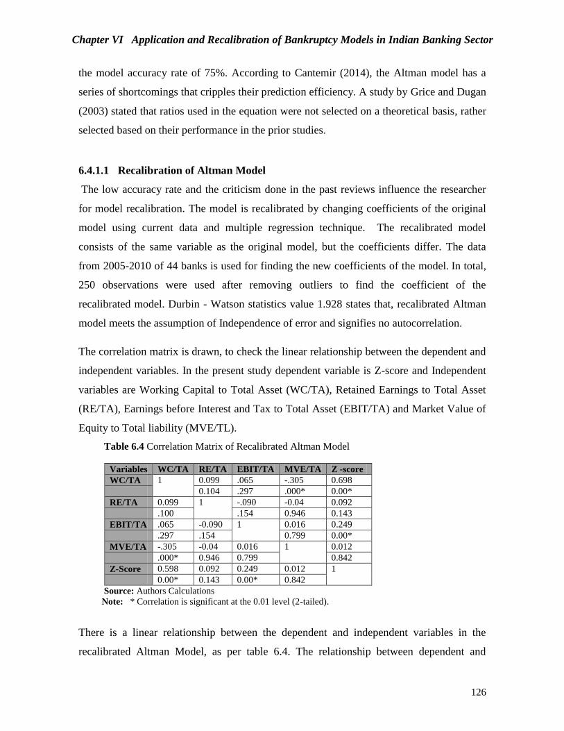
Chapter VI Application and Recalibration of Bankruptcy Models in Indian Banking Sector
126
the model accuracy rate of 75%. According to Cantemir (2014), the Altman model has a
series of shortcomings that cripples their prediction efficiency. A study by Grice and Dugan
(2003) stated that ratios used in the equation were not selected on a theoretical basis, rather
selected based on their performance in the prior studies.
6.4.1.1 Recalibration of Altman Model
The low accuracy rate and the criticism done in the past reviews influence the researcher
for model recalibration. The model is recalibrated by changing coefficients of the original
model using current data and multiple regression technique. The recalibrated model
consists of the same variable as the original model, but the coefficients differ. The data
from 2005-2010 of 44 banks is used for finding the new coefficients of the model. In total,
250 observations were used after removing outliers to find the coefficient of the
recalibrated model. Durbin - Watson statistics value 1.928 states that, recalibrated Altman
model meets the assumption of Independence of error and signifies no autocorrelation.
The correlation matrix is drawn, to check the linear relationship between the dependent and
independent variables. In the present study dependent variable is Z-score and Independent
variables are Working Capital to Total Asset (WC/TA), Retained Earnings to Total Asset
(RE/TA), Earnings before Interest and Tax to Total Asset (EBIT/TA) and Market Value of
Equity to Total liability (MVE/TL).
Table 6.4 Correlation Matrix of Recalibrated Altman Model
Variables WC/TA RE/TA EBIT/TA MVE/TA Z -score
WC/TA 1 0.099 .065 -.305 0.698
0.104 .297 .000* 0.00*
RE/TA 0.099 1 -.090 -0.04 0.092
.100 .154 0.946 0.143
EBIT/TA .065 -0.090 1 0.016 0.249
.297 .154 0.799 0.00*
MVE/TA -.305 -0.04 0.016 1 0.012
.000* 0.946 0.799 0.842
Z-Score 0.598 0.092 0.249 0.012 1
0.00* 0.143 0.00* 0.842
Source: Authors Calculations
Note: * Correlation is significant at the 0.01 level (2-tailed).
There is a linear relationship between the dependent and independent variables in the
recalibrated Altman Model, as per table 6.4. The relationship between dependent and

Chapter VI Application and Recalibration of Bankruptcy Models in Indian Banking Sector
127
independent variables is significant at a 1% level for the variable Z-score and WC/TA, Z-
score and EBIT/TA. The relationship among the Independent variable of the banks shows
the correlation coefficient value less than 0.70. This shows that there is no problem of
multicollinearity.
The third assumption of testing the outliers was checked with the help of casewise
diagnostics. Observations 118,120,124,213,221 are identified as unusual cases. Suitably
these outliers were removed. The homoscedasticity test shows residuals are randomly
scattered and observation to histogram satisfied the normality test. A histogram with a
superimposed normal curve depicts the normality of data, and PP-plot showed the
alignment of plots along with the diagonal line. This implies that there exists an
approximately linear pattern that depicts the consistency of the data with a normal
distribution. There was no problem with multicollinearity as the variance inflation factor
was less than five and the tolerance value was less than 0.2.
Table 6.5: Coefficient Test of Recalibrated Altman Model
Predictor Unstandardised
Coefficient
T-Value Sig.
Constant 2.22 2.219 0.27
WC/TA .754 17.405 .000*
RE/TA .036 .870 .385
EBIT/TA .199 4.829 .000*
MVE/ TL .239 5.553 .000*
Source: Authors Calculations based on Annexure Table A.40 - A.42
Note: Significance level – 1%*, ANNOVA F (4, 251) = 86.97, Sig = 0.00, Model Fitness: R= 0.763,
R2 = 0.582, AdjR2 = 0.575
Multiple linear regression was run to understand the coefficients of the equation for the
recalibrated model. Table 6.5 shows the results of regression analysis on public and private
sector banks data. The Results of regression show that adjusted R2 is 0.57 which means
that 57% of the variation in the dependent variable that is Z-score is due to the explanatory
variables (WC/TA, RE/TA, EBIT/TA and MVE/ TA) and remaining 43% variation is due
to other factors. F value is significant at 1%, hence we can say that the overall model is a
good fit. The value of beta (β) explains the contribution of the independent variable.
WC/TA shows the highest beta value, which means its contribution is more than other

Chapter VI Application and Recalibration of Bankruptcy Models in Indian Banking Sector
128
independent variables in Z-score. The above observations show the model fits the data well.
The recalibrated equation is as follows:
Recalibrated Equation of Altman Model
Z-scores = β+βX1+βX2+βX3+βX4.................................6.1
Z-scores = 2.22 + 0.754X1 + 0.036X2 + 0.199X3 + 0.239X4
Where X1 = Working capital/Total assets, X2 = Retained earnings/Total assets, X3 =
Earnings before interest and taxes/Total assets, X4= Market value equity/ Total liabilities
and Z = overall index.
6.4.1.2 Application of Recalibrated Altman Model
The recalibrated model is applied to 41 banks covering a period of 2011-2017. Three
merged banks were not taken in the sample of the recalibrated model as the recalibrated
model was applied for a period 2011 - 2017 and these three banks merged before 2011,
hence the data was not available between 2011 and 2017. The following table shows the
result of Recalibrated - Altman Model
Table 6.6: Results of Recalibrated Altman Model of 21 Public, 18 Private and 2 NWB
S.
N.
Public Banks
(Working Banks)
Score Result S.N
.
Private Banks (Working
Banks)
Score Result
1 Allahabad Bank 2.34 Grey 1 Axis Bank 2.33 Grey
2 Andhra Bank 2.31 Grey 2 Catholic Syrian Bank 2.30 Grey
3 Bank of Baroda 2.41 Grey 3 City Union Bank 2.34 Grey
4 Bank of India 2.33 Grey 4 DCB Bank 2.28 Grey
5 Bank of Maharashtra 2.30 Grey 5 Dhanalaxmi Bank 2.32 Grey
6 Canara Bank 2.32 Grey 6 Federal Bank 2.35 Grey
7 Central Bank of India 2.30 Grey 7 HDFC Bank 2.37 Grey
8 Corporation Bank 2.30 Grey 8 ICICI Bank 2.36 Grey
9 Dena Bank 2.30 Grey 9 Indusind Bank 2.41 Grey
10 IDBI 2.29 Grey 10 Jammu & Kashmir Bank 2.33 Grey
11 Indian Bank 2.30 Grey 11 Karnataka Bank 2.30 Grey
12 Indian Overseas Bank 2.32 Grey 12 Karur Vysya Bank 2.31 Grey
13 Oriental Bank of
Commerce 2.30 Grey
13 Kotak Mahindra Bank 2.35 Grey

Chapter VI Application and Recalibration of Bankruptcy Models in Indian Banking Sector
129
14 Punjab & Sind Bank 2.29 Grey 14 Lakshmi Vilas Bank Ltd. 2.29 Grey
15 Punjab National Bank 2.32 Grey 15 Nainital Bank 2.47 Grey
16 State Bank Of India 2.32 Grey 16 R B L Bank 2.34 Grey
17 Syndicate Bank 2.28 Grey 17 South Indian Bank 2.32 Grey
18 Uco Bank 2.31 Grey 18 Yes Bank 2.32 Grey
19 Union Bank Of India 2.31 Grey Non-Working Banks (NWB)
20 United Bank Of India 2.32 Grey 1 Bharat Overseas Bank (NWB) 0.98 Distress
21 Vijaya Bank 2.28 Grey 2 ING Vysya Bank (NWB) 1.14 Grey
Source: Authors calculations based on Appendix Table A.52
The tested recalibrated model shows all the working banks in the grey area, indicating the
firm’s likelihood of failure is less; however it also shows 50% of the NWB in the grey area.
These results draws the attention of the researcher on the predictive ability of this model
and hence identify the recalibrated model accuracy rate.
Table 6.7: Recalibrated Altman Model Accuracy Rate
Recalibrated Altman Error Rate Model Accuracy Rate
NWB Type I - 2% 98%
Working Banks Type II – 0%
Source: Authors calculations based on table 6.6
Note: Type I error- Prediction of NWB which will not go bankrupt, Type II error- Prediction of working
banks to be bankrupt
The recalibrated model accuracy rate applied to the present study shows an accuracy rate of
98%, whereas the original model applied to the present study shows an accuracy rate of
89%. This shows a difference in the accuracy rate of both models. This difference is
statistically checked with the help of an independent sample t-test. It is hypothesised for the
test that there are no statistical differences in the bankruptcy scores using the original and
the recalibrated bankruptcy models. The difference in these models may not arise, as both
models are using the same accounting variable to arrive at a score.

Chapter VI Application and Recalibration of Bankruptcy Models in Indian Banking Sector
130
Table no 6.8 - Result of Independent Sample T-test of Altman and Recalibrated Altman Model
Hypothesis P-value Decision
Mean Z-score of Altman Model = Mean Z-score of
Recalibrated Altman Model
0.000 Not supported
Source: Authors calculations based on Appendix table A.40, A.41, A.42 and A.52
The result of the independent sample t-test shows that there is a significant difference in the
mean of the original Altman and the mean of recalibrated Altman Model. These results fail
to accept the null hypothesis. The difference in the predictive ability between the two
models may be on account of environmental factors, industry conditions, country
conditions, period, etc. Thus, the model does not provide credible results under all
conditions. Further, since there is a significant difference in the Z-score of the original
Altman and recalibrated Altman model, a need felt to prove the accuracy of these models.
The accuracy of the model is checked based on a robust test.
6.4.1.3 Results of the Robust Tests
The robust test was conducted, taking into account profitability and asset quality as a
variable. These variables are measured using a proxy to a variable such as ROA and Net
NPA to Net Advances ratio, respectively. The objective of a robust test is to measure the
financial health of the banks in the current years. Therefore ROA and Net NPA to Net
Advance ratio for the year 2017 are considered. The robust test was calculated using the
data of 39 banks. The robust test was not conducted on non-working banks, as these banks
were merged before 2017 and the data about the same was not available. Based on these
ratios, the bases of discriminations have arrived. The bases of discrimination are shown in
Table 6.9
Table 6.9 Bases of discrimination as per Robust Test
Cases ROA and Net NPA to Net
Advance ratio
Zones
I R-score ≤ 1 Distress zone
II 1-2 A grey area
III 2-3 Safe zone
Source: Authors calculations based on Appendix table A.61

Chapter VI Application and Recalibration of Bankruptcy Models in Indian Banking Sector
131
The data on the ROA ratio is sorted in ascending order for 39 banks, which ranged from 0-
3. Based on the 0-3 range, three categories are made, such as (Safe, Grey and Distress zone)
to discriminate between banks. The score of ROA 0-3 is divided as 0-1.5 = distress zone,
1.5 - 2.5 = grey zone and 2.5 - 3.5 = safe zone. Higher the ratio reflects better profitability
positions of banks and vice versa.
The data on Net NPA to Net Advance ratio is sorted in descending order for thirty-nine
banks, which ranged from 0-15. Based on the 0-15 range, three categories are made, such
as (safe, grey and distress zone) to discriminate between banks. In this case score of Net
NPA to Net Advances ratio ranging from 0-14 is categorized as 0-5= Safe Zone, 5-10=Grey
Zone, and 10-15 = Distress Zone. Lower the ratio reflects better solvency position of banks
and vice versa.
Table 6.10: Results of tested Robust Test on 39 Indian banks.
S.
N.
Banks R-
Score
Result S.N. Banks R-
Score
Result
1 Allahabad Bank 1.5 Grey 21 Indusind Bank 3 Safe
2 Andhra Bank 2 Grey 22 Jammu & Kashmir Bank 2 Grey
3 Axis Bank 2.5 Safe 23 Karnataka Bank 2.5 Safe
4 Bank Of Baroda 2.5 Safe 24 Karur Vysya Bank 3 Safe
5 Bank Of India 1.5 Grey 25 Kotak Mahindra Bank 3 Safe
6 Bank Of Maharashtra 1 Distress 26 Lakshmi Vilas Bank 2.5 Safe
7 Canara Bank 2 Grey 27 Nainital Bank 1 Distress
8 Catholic Syrian Bank. 2 Grey
28 Oriental Bank of
Commerce 1.5 Grey
9 Central Bank Of India 1 Distress 29 Punjab & Sind Bank 2 Grey
10 City Union Bank 3 Safe 30 Punjab National Bank 2 Grey
11 Corporation Bank 2 Grey 31 R B L Bank 3 Safe
12 D C B Bank 2.5 Safe 32 South Indian Bank 2.5 Safe
13 Dena Bank 1.5 Grey 33 State Bank of India 2.5 Safe
14 Dhanlaxmi Bank. 2.5 Safe 34 Syndicate Bank 2 Grey
15 Federal Bank 2.5 Safe 35 UCO Bank 1.5 Grey
16 H D F C Bank 3 Safe 36 Union Bank Of India 2 Grey
17 I C I C I Bank 2.5 Safe 37 United Bank Of India 2 Grey
18 I D B I Bank 2 Grey 38 Vijaya Bank 2.5 Safe
19 -Indian Bank 2.5 Safe 39 Yes Bank. 3 Safe
20 Indian Overseas Bank 1 Distress
Source: Author's calculations based on appendix table A.6. Note: R-Score = Robust test score

Chapter VI Application and Recalibration of Bankruptcy Models in Indian Banking Sector
132
The result of the robust test shows four working banks under the distress category, stating a
90% accuracy rate. Further, the results of the original applied Altman and Recalibrated
Altman model are reconciled with a robust test by making comparisons amongst them.
Table 6.11: Comparison of Original and Recalibrated Altman Model with the Robust test
S.N
. Ba
nk
s
Alt
ma
n
Mo
del
Res
ult
Rec
ali
bra
te
d A
ltm
an
Mo
del
Res
ult
Dif
fere
nce
Ro
bu
st t
est
sco
re
Res
ult
1 Allahabad Bank 1.15 Grey 2.34 Grey 1.15 1.5 Grey
2 Andhra Bank 1.34 Grey 2.31 Grey 0.97 2 Grey
3 Axis Bank Ltd. 1.57 Grey 2.33 Grey 0.76 2.5 Safe
4 Bank Of Baroda 1.55 Grey 2.41 Grey 0.86 2.5 Safe
5 Bank Of India 1.28 Grey 2.33 Grey 1.05 1.5 Grey
6 Bank Of
Maharashtra 1.12 Grey 2.30 Grey 1.18 1 Distress
7 Canara Bank 1.35 Grey 2.32 Grey 0.97 2 Grey
8 Catholic Syrian
Bank 1.62 Grey 2.30 Grey 0.71 2 Grey
9 Central Bank Of
India 1.11 Grey 2.30 Grey 1.19 1 Distress
10 City Union Bank 1.46 Grey 2.34 Grey 0.88 3 Safe
11 Corporation
Bank 1.22 Grey 2.30 Grey 1.08 2 Grey
12 D C B Bank 1.18 Grey 2.28 Grey 1.1 2.5 Safe
13 Dena Bank 1.39 Grey 2.30 Grey 0.95 1.5 Grey
14 Dhanalaxmi
Bank 1.44 Grey 2.32 Grey 0.88 2.5 Safe
15 Federal Bank 1.58 Grey 2.35 Grey 0.77 2.5 Safe
16 H D F C Bank 1.40 Grey 2.37 Grey 0.97 3 Safe
17 I C I C I Bank 1.55 Grey 2.36 Grey 0.81 2.5 Safe
18 I D B I Bank 1.07 Distress 2.29 Grey 1.24 2 Grey-----1st
case
19 -Indian Bank 1.19 Grey 2.30 Grey 1.11 2.5 Safe
20 Indian Overseas
Bank 1.27 Grey 2.32 Grey 1.05 1 Distress
21 Indusind Bank 1.46 Grey 2.41 Grey 0.89 3 Safe
22 Jammu &
Kashmir Bank 1.49 Grey 2.33 Grey 0.81 2 Grey
23 Karnataka Bank 1.39 Grey 2.30 Grey 0.91 2.5 Safe
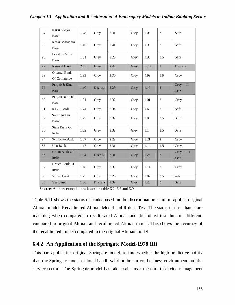
Chapter VI Application and Recalibration of Bankruptcy Models in Indian Banking Sector
133
24 Karur Vysya
Bank 1.28 Grey 2.31 Grey 1.03 3 Safe
25 Kotak Mahindra
Bank 1.46 Grey 2.41 Grey 0.95 3 Safe
26 Lakshmi Vilas
Bank 1.31 Grey 2.29 Grey 0.98 2.5 Safe
27 Nainital Bank 2.65 Grey 2.47 Grey -0.18 1 Distress
28 Oriental Bank
Of Commerce 1.32 Grey 2.30 Grey 0.98 1.5 Grey
29 Punjab & Sind
Bank 1.10 Distress 2.29 Grey 1.19 2
Grey----II
case
30 Punjab National
Bank 1.31 Grey 2.32 Grey 1.01 2 Grey
31 R B L Bank 1.74 Grey 2.34 Grey 0.6 3 Safe
32 South Indian
Bank 1.27 Grey 2.32 Grey 1.05 2.5 Safe
33 State Bank Of
India 1.22 Grey 2.32 Grey 1.1 2.5 Safe
34 Syndicate Bank 1.07 Grey 2.28 Grey 1.21 2 Grey
35 Uco Bank 1.17 Grey 2.31 Grey 1.14 1.5 Grey
36 Union Bank Of
India 1.04 Distress 2.31 Grey 1.25 2
Grey----III
case
37 United Bank Of
India 1.18 Grey 2.32 Grey 1.14 2 Grey
38 Vijaya Bank 1.25 Grey 2.28 Grey 1.07 2.5 safe
39 Yes Bank 1.06 Distress 2.32 Grey 1.26 3 Safe
Source: Authors compilations based on table 6.2, 6.6 and 6.9
Table 6.11 shows the status of banks based on the discrimination score of applied original
Altman model, Recalibrated Altman Model and Robust Test. The status of three banks are
matching when compared to recalibrated Altman and the robust test, but are different,
compared to original Altman and recalibrated Altman model. This shows the accuracy of
the recalibrated model compared to the original Altman model.
6.4.2 An Application of the Springate Model-1978 (II)
This part applies the original Springate model, to find whether the high predictive ability
that, the Springate model claimed is still valid in the current business environment and the
service sector. The Springate model has taken sales as a measure to decide management

Chapter VI Application and Recalibration of Bankruptcy Models in Indian Banking Sector
134
capability to deal with competition, however, in the present study in place of sales, total
income is taken as an indicator. In the present study, the Springate model was applied to 44
public, private and non-working banks.
Table 6.12: Results of the applied Springate model on 21 public 18 private and 5 NWB
S.N. Public Banks (Working
Banks) S-Score Result S.N.
Private Banks (Working
banks)
S-
Score Result
1 Allahabad Bank 2.23 Safe 1 Axis Bank Ltd. 1.67 Safe
2 Andhra Bank 2.20 Safe 2 Catholic Syrian Bank 2.33 Safe
3 Bank Of Baroda 1.64 Safe 3 City Union Bank 2.11 Safe
4 Bank Of India 1.82 Safe 4 DCB Bank 1.34 Safe
5 Bank Of Maharashtra 1.79 Safe 5 Dhanalaxmi Bank 1.99 Safe
6 Canara Bank 2.06 Safe 6 Federal Bank 2.34 Safe
7 Central Bank Of India 1.62 Safe 7 HDFC Bank 0.95 Safe
8 Corporation Bank 1.87 Safe 8 ICICI Bank 1.28 Safe
9 Dena Bank 2.19 Safe 9 Indusind Bank 1.78 Safe
10 IDBI Bank Ltd. 1.81 Safe 10 Jammu & K Bank 2.13 Safe
11 Indian Bank 1.69 Safe 11 Karnataka Bank 2.48 Safe
12 Indian Overseas Bank 2.05 Safe 12 Karur Vysya Bank 2.36 Safe
13 Oriental Bank Of Comm. 2.23 Safe 13 Kotak Mahindra Bank 1.21 Safe
14 Punjab & Sind Bank 2.44 Safe 14 Lakshmi Vilas Bank 2.00 Safe
15 Punjab National Bank 1.76 Safe 15 Nainital Bank 1.79 Safe
16 State Bank Of India 0.94 Safe 16 R B L Bank 1.60 Safe
17 Syndicate Bank 1.78 Safe 17 South Indian Bank 2.20 Safe
18 Uco Bank 1.98 Safe 18 Yes bank 1.23 Safe
19 Union Bank Of India 2.04 Safe Non-Working Banks (NWB)
20 United Bank Of India 1.77 Safe 1 Bank Of Punjab (NWB) 1.42 safe
21 Vijaya Bank 2.30 Safe 2 Bank Of Rajasthan. (NWB) 1.14 safe
3 Bharat Overseas. Bank Ltd.
(NWB)
1.81 safe
4 Centurion Bank Of Punjab
Ltd. (NWB)
0.92 safe
5 ING Vysya Bank (NWB) 1.14 safe
Source: Authors calculations based on Appendix table A.43-A.45
As per the results in table 6.6, shows all the good banks in the grey area indicating the
firm's likelihood of failure is less; however it also shows 50% of the NWB in the grey area.

Chapter VI Application and Recalibration of Bankruptcy Models in Indian Banking Sector
135
These results draw the attention of the researcher on the predictive ability of this model and
hence identify the recalibrated model accuracy rate.
In table 6.12 the Springate model shows all the working public and private banks in a safe
position, however this model also shows the NWB in the safe position, this drives the
researcher to check the accuracy of this model.
Table 6.13: Model Accuracy Rate of Springate Model
Springate model Error Rate Model Accuracy Rate
NWB Type I -11% 89%
Working Banks Type II -0%
Source: Authors calculations based on the results of Table 6.12
Note: Type I error- Prediction of NWB which will not go bankrupt, Type II error - Prediction of
working banks to be bankrupt
The model’s accuracy rate was calculated by finding out Type I and Type II error in
predicting the bankruptcy of banks. Table 6.13 shows the error rate of 11% and an accuracy
rate of 89%. This model failed to predict the bankruptcy of NWB correctly. As per this
model, all the NWB banks fall in the safe category. Therefore, this model needs revision.
As evidence of this fact, a study by Sajjan (2016) compared the result of investigating two
models Zavgren and Springate. The results indicate the adjusted Springate model was
efficient than another model in the bankruptcy year. This suggests the need for
recalibrations of this model.
6.4.2.1 Recalibration of Springate Model
The criticism has done of the Springate model in past studies and the error present in the
tested model drives the researcher for recalibration of the model. The model is recalibrated
by changing coefficients of the original model using current data and multiple regression
technique. The recalibrated model consists of the same variable as the original model, but
the coefficients differ. The data from 2005-2010 of 44 banks is used for finding the new
coefficients of the model. In total, 239 observations were used after removing suitable
outliers, to find the coefficient of the recalibrated model. Durbin- Watson statistics value
1.84 states that, recalibrated Springate model meets the assumption of Independence of
error and signifies no autocorrelation.

Chapter VI Application and Recalibration of Bankruptcy Models in Indian Banking Sector
136
The correlation matrix is drawn to check the linear relationship between the dependent and
independent variables. In the present study dependent variable is S-score and Independent
variables are Working Capital to Total Asset (WC/TA), Earnings before Interest and Tax to
Total Asset to Total Asset ratio (EBIT/TA), Earnings before Interest and Tax to Current
Liability (EBIT/CL) and Total Income to Total Asset (TI/TA).
Table 6.14: Correlation Matrix of Recalibrated Springate Model
Variables WC/TA EBIT/TA EBIT/CL TI/TA S-score
WC/TA 1 0.033 0.232 -0.108 0.391
0.302 0.000** 0.048 0.00**
EBIT/TA 0.033 1 0.456 0.715 0.493
0.302 0.00** 0.00** 0.00**
EBIT/CL 0.232 0.456 1 0.146 0.930
0.000** 0.000 0.012* 0.00**
TI/TA -0.108 0.715 0.146 1 0.930
0.048 0.00** 0.012* 0.00**
S-score 0.391 0.493 0.930 0.165 1
0.00** 0.00** 0.00** 0.005**
Source: Authors Calculations. Notes: *Correlation at 5% ** Correlation at 1%
There is a linear relationship between the dependent and independent variables in the
recalibrated Springate Model, as per table 6.14. There exists a strong positive relationship
between S-score and ‘EBIT/CL’. It may be strong because the difference in the values of
EBIT to CL is very less; hence the final value of the ratio is more. This makes a high
correlation between these two variables; however with the other independent variables,
there exists a moderate positive relationship with the dependent variable. As evidence of
this fact, Warastuti (2014), in its study, removed this ratio of EBIT/CL from the model
since it has a problem of multicollinearity. Its study also says that variable EBIT and
working capital have a significant positive impact on the health of the bank, whereas the
other two variables have less impact on the dependent variable. The relationship among the
Independent variable of the banks shows the correlation coefficient value less than 0.70.
This shows that there is no problem of multicollinearity. The relationship between the
independent variables is significant at 5% and 1% level of significance concerning all
variables except for WC/TA to EBIT/TA.

Chapter VI Application and Recalibration of Bankruptcy Models in Indian Banking Sector
137
This model satisfies the assumption of linearity between the dependent and independent
variables after the transformation of data. Before the transformation of data, a partial
regression plot shows a partial relationship between S-score and WC/TA, TI/TA, EBIT/TA,
and a perfect relationship between S-score and EBIT/CL. The linear relationship between
the dependent and Independent variable was also checked collectively, by checking the
studentized residuals value against unstandardized predicted value. There is a linear
relationship between the independent and dependent variables. This model shows a
satisfactory VIF and tolerance level, signifying an absence of multicollinearity. The outliers
present in the model were removed. The assumption of Homoscedasticity states that the
residuals are equal for all the values of the predicted dependent variable. The residuals in
the recalibrated model appear randomly scattered, on this basis, it would appear that the
assumption of Homoscedasticity has been met. The assumption of Normality is checked
with the help of a Histogram and PP-plot. In this case, a histogram with a superimposed
normal curve depicts the normality of data, and PP-plot shows the alignment of plots along
with the diagonal line, which also signals the normality of data. This implies that there
exists an approximately linear pattern that depicts the consistency of the data with a normal
distribution.
Table 6.15: The Coefficient test of Recalibrated Springate Model
Source: Authors calculations based on the annexure Table A.43, A.44 and A.45
Note: Durbin Watson Test: 1.847, Homoscedasticity Test: residuals are randomly scattered, ANOVA value-
F (4, 239) =597.38, Sig = 0.00 Model Fitness: R= 0.931 R2 = 0.891, AdjR2 = 0.872
Multiple linear regression was run to understand the coefficients of the equation for the
recalibrated model. Table 6.15 shows the results of regression analysis on public and
private sector bank's data. The Results of regression show that adjusted R2 is 0.87 which
S.N. Predictor Unstandardised
Coefficient
T-value Sig
Constant .093 1.298 .195
1 WC/TA 1.371 9.942 .000
2 EBIT/TA 7.124 5.015 .000
3 EBIT/CL .585 34.444 .000
4 TI/TA .999 1.686 .093

Chapter VI Application and Recalibration of Bankruptcy Models in Indian Banking Sector
138
means that 87% of the variation in the dependent variable i.e., S-score is due to the
explanatory variables (WC/TA, EBIT/TA, EBIT/CL and TI/TA) and remaining 13%
variation is due to other factors. F value is significant at 1% hence, we can say that the
overall Model is a good fit. The value of beta (β) explains the contribution of the
independent variable. EBIT/TA shows the highest beta value, which means its contribution
is more than other independent variables in S-score. The above observations show the
model fits the data well. The recalibrated equation is as follows:
Recalibrated Equation of Springate Model
S-scores = β +β1X1+β2X2+β3X3+β4X4.........................(6.2)
S-scores = 0.093 + 1.37X1 + 7.124X2 + 0.585X3 - 1.988X4
Where X1 = Working capital/Total Assets, X2 = Earnings before Interest and Tax/Total
Assets, X3 = Earnings before interest and taxes/Current Liability, X4 = Total Income/Total
Asset, and S= overall index.
6.4.2.2 Application of Recalibrated Springate Model
The recalibrated model is applied to 41 banks covering a period of 2011-2017. Three
merged banks were not taken in the sample of the recalibrated model as the recalibrated
model was applied for a period 2011 -2017, and these three banks merged before 2011,
hence the data was not available between 2011 and 2017. The following table shows the
result of Recalibrated - Springate Model
Table 6.16: Results of Applied Recalibrated Model on 21 Public, 18 Private and 2 NWB S.
N.
Public Banks
(Working Banks)
S-score Result S.
N.
Private Banks
(Working Banks)
S-
score
Result
1 Allahabad Bank 3.06 Safe 1 Axis Bank Ltd. 2.76 Safe
2 Andhra Bank 3.12 Safe 2 Catholic Syrian Bank
Ltd. 3.08
Safe
3 Bank Of Baroda 2.36 Safe 3 City Union Bank Ltd. 3.14 Safe
4 Bank Of India 2.57 Safe 4 DCB Bank Ltd. 0.77 Distress
5 Bank Of Maharashtra 2.64 Safe 5 Dhanalaxmi Bank Ltd. 2.73 Safe
6 Canara Bank 2.83 Safe 6 Federal Bank Ltd. 3.12 Safe
7 Central Bank Of India 2.49 Safe 7 H D F C Bank Ltd. 5.01 Safe
8 Corporation Bank 3.17 safe 8 ICICI Bank Ltd. 2.65 Safe
9 Dena Bank 3.10 Safe 9 Indusind Bank Ltd. 2.95 Safe
10 I D B I Bank Ltd. 2.84 Safe
10 Jammu & Kashmir
Bank Ltd. 2.94
Safe

Chapter VI Application and Recalibration of Bankruptcy Models in Indian Banking Sector
139
11 -Indian Bank 2.77 Safe 11 Karnataka Bank Ltd. 3.18 Safe
12 Indian Overseas Bank 2.88 Safe 12 Karur Vysya Bank Ltd. 3.39 Safe
13 Oriental Bank Of
Commerce 3.21
Safe 13
Kotak Mahindra Bank
Ltd. 0.80
Distress
14 Punjab & Sind Bank 3.66 Safe
14 Lakshmi Vilas Bank
Ltd. 3.11
Safe
15 Punjab National Bank 2.82 Safe 15 Nainital Bank Ltd. 2.47 Safe
16 State Bank Of India 2.15 Safe 16 R B L Bank Ltd. 2.55 Safe
17 Syndicate Bank 2.58 Safe 17 South Indian Bank Ltd. 3.06 Safe
18 Uco Bank 2.42 Safe 18 Yes Bank Ltd. 0.45 Distress
19 Union Bank Of India 2.99 Safe Non - Working Banks (NWB)
20 United Bank Of India 2.49 Safe 1 Bharat Overseas. Bank
Ltd. (NWB)
1.92 safe
21 Vijaya Bank 3.21 Safe
2 ING Vysya Bank Ltd.
(NWB)
1.34 safe
Source: Authors calculations based on the appendix table A.53
The tested recalibrated model shows three working banks in the financial distress position
and all NWB banks in a safe position. These results drive the researcher to check the
recalibrated model's accuracy rate.
Table 6.17: Model Accuracy Rate of Recalibrated Springate Model
Recalibrated Springate Model Error Rate Model Accuracy Rate
NWB Type I - 5% 88%
Working Banks Type II - 7%
Source: Authors calculations based on table 5.19 Note: Type I error- Prediction of NWB which will not go bankrupt, Type II error - Prediction of working banks to be
bankrupt
The model’s accuracy rate was calculated by finding out Type I and Type II error in
predicting the bankruptcy of banks. Table 6.17 shows the total error rate of 12%. The
recalibrated Springate model has an accuracy rate of 88%, which is low compared to the
accuracy rate of the original Springate model. The recalibrated Springate model shows
three private banks in the distress position however the same banks are safe in the original
Springate model. Also, the scores calculated in the recalibrated model are higher than that
of the original model. This is due to the higher coefficients of the recalibrated model. This
shows a difference in the recalibrated and the original model. Thus the results of the tested
Springate model and the tested recalibrated Springate model differ concerning 5% of banks
in a sample. To prove this difference, a statistical method such as an Independent sample t-
test was conducted. It is hypothesised for the test that there are no statistical differences in
the bankruptcy scores using the original and the recalibrated bankruptcy models. The

Chapter VI Application and Recalibration of Bankruptcy Models in Indian Banking Sector
140
difference in these models may not arise, as both models are using the same accounting
variable to arrive at a score. The result of the T-test is as follows:
Table no 6.18 - Result of Independent Sample T-test of Springate and Recalibrated Springate Model
Hypothesis P-value Decision
Mean S - score of Springate Model = Mean S - score of Recalibrated
Springate Model
0.000 Not supported
Source: Authors calculations based on appendix table A.43, A.44, A.45 and A.53
The result of the independent sample t-test shows a significant difference in the bankruptcy
scores of the original Springate and the recalibrated Springate model. These results fail to
accept the null hypothesis. The difference in the predictive ability between the two models
may be on account of environmental factors, industry conditions, country conditions,
period, etc. Thus, the model does not provide credible results under all conditions. Further,
since there is a significant difference in the S-score of the original Springate and
recalibrated Springate model, a need felt to prove the predictive ability of these models.
The predictive ability of the model is checked based on a robust test. The result and the
bases of discrimination for a robust test are shown in table 6.9 and 6.10, respectively.
6.4.2.3 Comparison of original and Recalibrated Springate Model with the Robust test
The results of the original Springate recalibrated Springate model is compared with the
robust test to judge the accuracy of the model
Table 6.19: Comparison of original and Recalibrated Springate Model with the Robust test S
. N.
Ba
nk
s
Orig
ina
l
Mo
del
Decisio
n
Reca
libra
te
d M
od
el
Decisio
n
Differen
ce
Ro
bu
st test
Decisio
n
1 Allahabad Bank 2.23 Safe 3.06 Safe 1.15 1.5 Safe
2 Andhra Bank 2.20 Safe 3.12 Safe 0.97 2 Safe
3 Axis Bank 1.67 Safe 2.76 Safe 0.76 2.5 Safe
4 Bank Of Baroda 1.64 Safe 2.36 Safe 0.86 2.5 Safe
5 Bank Of India 1.82 Safe 2.57 Safe 1.05 1.5 Safe
6 Bank Of Maharashtra 1.79 Safe 2.64 Safe 1.18 1 Safe
7 Canara Bank 2.06 Safe 2.83 Safe 0.97 2 Safe

Chapter VI Application and Recalibration of Bankruptcy Models in Indian Banking Sector
141
8 Catholic Syrian Bank 2.33 Safe 3.08 Safe 0.71 2 Safe
9 Central Bank Of India 1.62 Safe 2.49 Safe 1.19 1 Safe
10 City Union Bank 2.11 Safe 3.14 Safe 0.88 3 Safe
11 Corporation Bank 1.87 Safe 3.17 Safe 1.08 2 Safe
12 D C B Bank 1.34 Safe 0.77 FD 1.1 2.5 Safe
13 Dena Bank 2.19 Safe 3.10 Safe 0.95 1.5 Safe
14 Dhanlaxmi Bank 1.34 Safe 2.73 Safe 0.88 2.5 Safe
15 Federal Bank 2.34 Safe 3.12 Safe 0.77 2.5 Safe
16 H D F C Bank 0.95 Safe 5.01 Safe 0.97 3 Safe
17 I C I C I Bank 1.28 Safe 2.65 Safe 0.81 2.5 Safe
18 I D B I Bank 1.81 Safe 2.84 Safe 1.24 2 Safe
19 -Indian Bank 1.69 Safe 2.77 Safe 1.11 2.5 Safe
20 Indian Overseas Bank 2.05 Safe 2.88 Safe 1.05 1 Safe
21 Indusind Bank 1.78 Safe 2.95 Safe 0.89 3 Safe
22 Jammu & Kashmir
Bank 2.13
Safe 2.94
Safe 0.81 2
Safe
23 Karnataka Bank 2.48 Safe 3.18 Safe 0.91 2.5 Safe
24 Karur Vysya Bank 2.36 Safe 3.39 Safe 1.03 3 Safe
25 Kotak Mahindra Bank 1.21 Safe 0.80 FD 0.95 3 Safe
26 Lakshmi Vilas Bank 2.00 Safe 3.11 Safe 0.98 2.5 Safe
27 Nainital Bank 1.79 Safe 2.47 Safe -0.18 1 Safe
28 Oriental Bank of
Commerce 2.23
Safe 3.21
Safe 0.98 1.5
Safe
29 Punjab & Sind Bank 2.44 Safe 3.66 Safe 1.19 2 Safe
30 Punjab National Bank 1.76 Safe 2.82 Safe 1.01 2 Safe
31 R B L Bank 1.60 Safe 2.55 Safe 0.6 3 Safe
32 South Indian Bank 2.20 Safe 3.06 Safe 1.05 2.5 Safe
33 State Bank Of India 0.94 Safe 2.15 Safe 1.1 2.5 Safe
34 Syndicate Bank 1.78 Safe 2.58 Safe 1.21 2 Safe
35 Uco Bank 1.98 Safe 2.42 Safe 1.14 1.5 Safe
36 Union Bank of India 2.04 Safe 2.99 Safe 1.25 2 Safe
37 United Bank of India 1.77 Safe 2.49 Safe 1.14 2 Safe
38 Vijaya Bank 2.30 Safe 3.21 Safe 1.07 2.5 Safe
39 Yes Bank 1.23 Safe 0.45 FD 1.26 3 Safe
Source: Authors Compilation of data based on Table 6.9, 6.12 and 6.16

Chapter VI Application and Recalibration of Bankruptcy Models in Indian Banking Sector
142
Table 6.19 shows the status of banks based on the discrimination score of applied original
Springate model, Recalibrated Springate Model and Robust Test. The results of the three
cases are different when compared to the robust test and recalibrated Springate model but
are matching when compared to the original Springate and the robust test. This shows the
accuracy of the original Springate model compared to the recalibrated Springate model,
evidenced by the fact of the accuracy rate of both models. Overall the results show original
Springate model performs better than the recalibrated Springate model, hence it can be
concluded that original Springate model works better in the country of its origin as it shows
93% accuracy rate in their own country, but it proves a less accurate in some other country
as the economic conditions differ from country to country. Also, the original model shows
less accuracy rate due to its sample bias - as originally it was applied for the manufacturing
firms. Still, in the present study, it is used in the service sector.
6.4.3 Application of Zmijewski Model - 1984 (III)
This part applies the original Zmijewski model, to find whether the high predictive ability
that, Zmijewski model claimed is still valid in the current business environment and service
sector. In the present study, the Zmijewski model was applied to 41 public, private and
non-working banks. Table 6.20 shows the X-score and probability of bankruptcy of the
respective bank.
Table 6.20: Result of the tested Zmijewski model on 21 public, 18 private and 2 NWB
S. N
.
Pu
blic
Ba
nk
s
(Wo
rkin
g
Ba
nk
s)
X-S
core
Pro
ba
bility
Decisio
n
S. N
.
Priv
ate
ba
nk
s
(Wo
rkin
g
ba
nk
s)
X-S
core
Pro
ba
bility
Decisio
n
1 Allahabad Bank -3.09 0.1
1
Safe 1 Axis Bank -4.32 0.1
0
Safe
2 Andhra Bank -3.87 0.0
9
Safe 2 Catholic Syrian
Bank
-0.05 0.3
0
Safe
3 Bank Of Baroda -4.81 0.0
1
Safe 3 City Union Bank -4.43 0.1
5
Safe
4 Bank Of India -2.74 0.0
6
Safe 4 D C B Bank 6.89 1.0
0
Distress
5 Bank Of
Maharashtra
-1.82 0.1
8
Safe 5 Dhanalaxmi Bank -0.59 0.2
6
Safe
6 Canara Bank -3.21 0.0
2
Safe 6 Federal Bank -3.27 0.1
1
Safe
7 Central Bank Of
India
-1.12 0.2
7
Safe 7 H D F C Bank -4.87 0.1
5
Safe

Chapter VI Application and Recalibration of Bankruptcy Models in Indian Banking Sector
143
Source: Authors calculations based on appendix table A.46, A.47, and A.48
The results of the application of the Zmijewski model show that in the case of public sector
banks, most of the banks fall in the safe area with the exception of one bank in distress zone
whose probability of bankruptcy is 69%. Similarly, in the case of private banks, the
majority of them are in a safe area, and two banks lie in distress position whose probability
of bankruptcy is more than 50%. The probability of bankruptcy is very high for the DCB
bank. In the case of NWB, four banks are in the distressed zone, and only one bank is in the
safe category. The NWB in the distressed zone has a higher probability of bankruptcy.
These results reflect certain working banks in the distress position and NWB in the safe
zone. This draws the attention of the researcher to find the accuracy rate of the model. This
accuracy rate was found out by seeking Type I and Type II error.
8 Corporation Bank -3.03 0.0
9
Safe 8 I C I C I Bank -3.29 0.2
3
Safe
9 Dena Bank -1.8 0.1
6
Safe 9 Indusind Bank 0.25 0.6
1
Distress
1
0
I D B I Bank 1.26 0.6
9
Distress 10 Jammu & Kashmir
Bank
-3.94 0.1
6
Safe
1
1
Indian Bank -1.24 0.2
3
Safe 11 Karnataka Bank -2.48 0.0
1
Safe
1
2
Indian Overseas
Bank
-2.71 0.3
2
Safe 12 Karur Vysya Bank -3.30 0.1
9
Safe
1
3
Oriental Bank of
Commerce
-1.72 0.2
0
Safe 13 Kotak Mahindra
Bank
-6.73 0.3
1
Safe
1
4
Punjab & Sind
Bank
-1.69 0.3
1
Safe 14 Lakshmi Vilas
Bank
-2.01 0.3
0
Safe
1
5
Punjab National
Bank
-2.47 0.1
5
Safe 15 Nainital Bank -4.42 0.1
5
Safe
1
6
State Bank of
India
-1.93 0.2
3
Safe 16 R B L Bank -1.53 0.2
8
Safe
1
7
Syndicate Bank -3.15 0.0
9
Safe 17 South Indian Bank -3.48 0.2
3
Safe
1
8
UCO Bank -1.82 0.1
7
Safe 18 Yes Bank -2.85 0.3
0
Safe
1
9
Union Bank Of
India
-1.95 0.1
8
Safe Non-Working Banks (NWB)
2
0
United Bank Of
India
-2.16 0.3
5
Safe 1 Bank Of Punjab
[NWB] 7.02 1.0
0
Distress
2
1
Vijaya Bank -1.07 0.2
4
Safe 2 Bank Of Rajasthan
[NWB] -0.76 0.2
0
Safe
3 Bharat Overseas
Bank [NWB] 2.07 0.9
8
Distress
4 Centurion Bank Of
Punjab [NWB] 2.45 0.9
9
Distress
5 I N G Vysya Bank
[NWB] 0.02 0.5
1
Distress
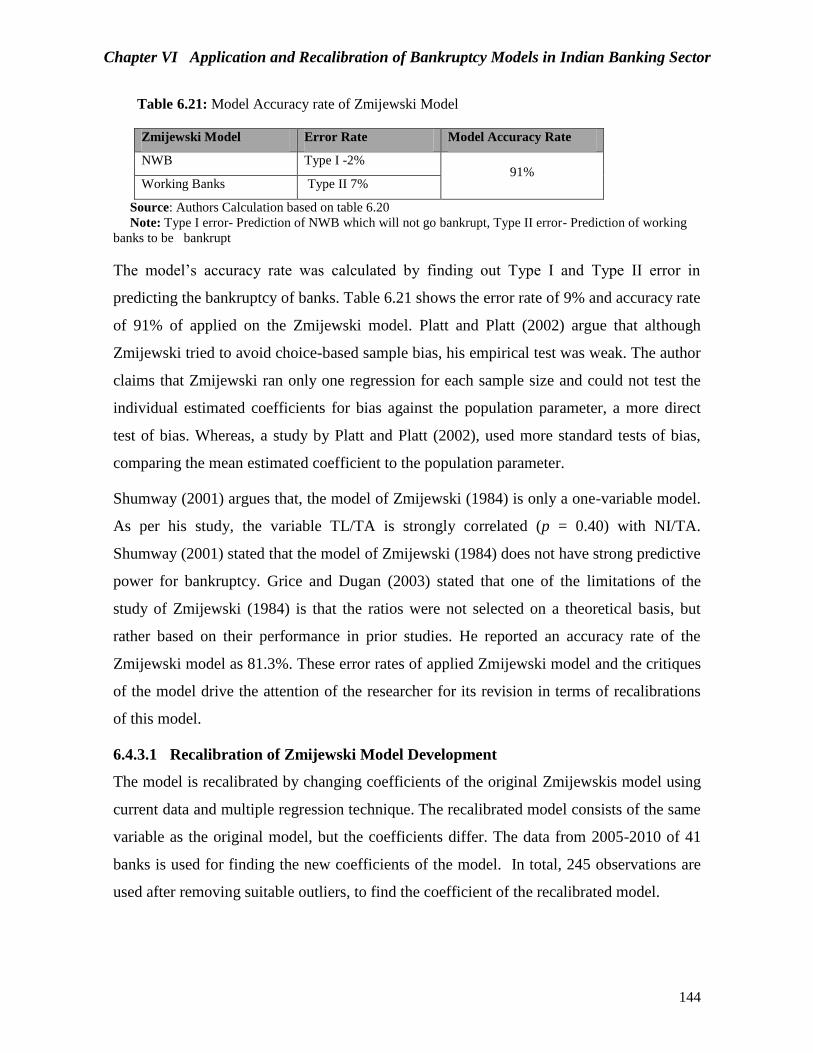
Chapter VI Application and Recalibration of Bankruptcy Models in Indian Banking Sector
144
Table 6.21: Model Accuracy rate of Zmijewski Model
Zmijewski Model Error Rate Model Accuracy Rate
NWB Type I -2% 91%
Working Banks Type II 7%
Source: Authors Calculation based on table 6.20
Note: Type I error- Prediction of NWB which will not go bankrupt, Type II error- Prediction of working
banks to be bankrupt
The model’s accuracy rate was calculated by finding out Type I and Type II error in
predicting the bankruptcy of banks. Table 6.21 shows the error rate of 9% and accuracy rate
of 91% of applied on the Zmijewski model. Platt and Platt (2002) argue that although
Zmijewski tried to avoid choice-based sample bias, his empirical test was weak. The author
claims that Zmijewski ran only one regression for each sample size and could not test the
individual estimated coefficients for bias against the population parameter, a more direct
test of bias. Whereas, a study by Platt and Platt (2002), used more standard tests of bias,
comparing the mean estimated coefficient to the population parameter.
Shumway (2001) argues that, the model of Zmijewski (1984) is only a one-variable model.
As per his study, the variable TL/TA is strongly correlated (p = 0.40) with NI/TA.
Shumway (2001) stated that the model of Zmijewski (1984) does not have strong predictive
power for bankruptcy. Grice and Dugan (2003) stated that one of the limitations of the
study of Zmijewski (1984) is that the ratios were not selected on a theoretical basis, but
rather based on their performance in prior studies. He reported an accuracy rate of the
Zmijewski model as 81.3%. These error rates of applied Zmijewski model and the critiques
of the model drive the attention of the researcher for its revision in terms of recalibrations
of this model.
6.4.3.1 Recalibration of Zmijewski Model Development
The model is recalibrated by changing coefficients of the original Zmijewskis model using
current data and multiple regression technique. The recalibrated model consists of the same
variable as the original model, but the coefficients differ. The data from 2005-2010 of 41
banks is used for finding the new coefficients of the model. In total, 245 observations are
used after removing suitable outliers, to find the coefficient of the recalibrated model.

Chapter VI Application and Recalibration of Bankruptcy Models in Indian Banking Sector
145
To develop a recalibrated Zmijewski model, all the assumptions required to run regression
were checked. Durbin- Watson statistics value 1.21 states that, recalibrated Zmijewski
model meets the assumption of Independence of error and signifies no autocorrelation. The
assumption linear relationship between the dependent and independent variables is tested
with the help of the correlation matrix.
Table 6.22: Correlation Matrix of Zmijewski Model
Variables ROA TD/TA CA/CL X-score
ROA 1 -0.374 -.003 -0.661
0.00 .480 .000**
TD/TA -0.374 1 0.261 0.274
0.00 0.00 0.00
CA/CL -.003 0.261 1 -0.25
.480 0.00 .348
X-Score -0.661 0.274 -0.25 1
.000** 0.00 .348
Source: Authors Calculations Notes:*Correlation at 5%** Correlation at 1%
In the above table, the dependent variable is X-score and the independent variables are
Return on Assets (ROA), Total Liabilities/Total Assets (TL/TA), Current Assets / Current
Liabilities(CA/CL). The relationship between the dependent and independent variables is
verified at 1% and 5% level of significance. Table 6.22 shows the existence of a strong
negative relationship between X-score and ‘ROA’, and it signifies an increase in the ROA
will decrease the X-score. However, it may be strong because the difference in the values
of EBIT to CL is very less; hence the final value of the ratio is more. The relationship of X-
score with the other independent variables is negative and weak. Hence smaller the X-
score better for the bank to avoid bankruptcy. In other words, negative the X-score, lesser
the chance for the bank to go bankrupt. The relationship among the independent variable of
the banks shows the correlation coefficient value less than 0.70. This shows that there is no
problem of multicollinearity.
The value of VIF in the regression output is one, and the value of tolerance is less than 1 for
all the independent variables. This depicts that there is no multicollinearity in the
recalibrated model. The outliers are indicated by the points in the upper-right corner of the
plot. Observations 226,228,229,231,232,234,237,243 and 246 are identified as unusual

Chapter VI Application and Recalibration of Bankruptcy Models in Indian Banking Sector
146
cases because the absolute value of the standardized residuals is greater than 2. These
outliers were removed. The residuals in the recalibrated model appear randomly scattered;
on this basis, it would appear that the assumption of Homoscedasticity has been met. A
histogram with a superimposed normal curve and PP-plot, along with the diagonal line,
depicts the normality of data. This implies that there exists an approximately linear pattern
that depicts the consistency of the data with a normal distribution.
Table 6.23: Coefficient Test of Zmijewski Model
Predictor Unstandardised
Coefficient
T-value Sig
Constant -2.534 -5.10 .610
ROA -3.79 -12.370 .000
TD/TA 4.36 .781 .435
CA/CL -.081 -.759 .448
Source: Authors calculations based on annexure A.46, A.47 and A.48
Note: Durbin Watson Test-1.21, Homoscedasticity Test: residuals are randomly scattered, ANOVA
value-F (3,242) =6322, Sig = 0.000, Model Fitness: R= 0.663, R2 = 0.439 AdjR2 = 0.432
Multiple linear regression was run to understand the coefficients of the equation for the
recalibrated model. Table 6.23 shows the results of regression analysis on public and
private sector banks data. The Results of regression show that adjusted R2 is 0.43, which
means that 47% of the variation in the dependent variable i.e., X-score is due to the
explanatory variables (ROA, TD/TA and CA/CL) and remaining 57% variation is due to
other factors. F-value is significant at 1% hence, we can say that the overall Model is good
fit. The value of beta (β) explains the contribution of the independent variable. ‘TD/TA’
shows the highest beta value, which means its contribution is more than other independent
variables in X-score. The above observations show the model fits the data well. The
recalibrated equation is as follows:
Recalibrated Equation of Zmijewski Model
X-scores =β +β1X1+β2X2-β3X3............................. (6.3)
X-scores = -2.534 - 3.79X1 + 4.246X2 - 0.081X3
Where X1 = Return on Asset (ROA), X2 = Total deposit to Total Asset, X3 = Current Asset
to Current Liabilities and X-Score = Overall index.

Chapter VI Application and Recalibration of Bankruptcy Models in Indian Banking Sector
147
6.4.3.2 Application of Recalibrated Zmijewski Model
The recalibrated Zmijewski model was applied on 41public and private banks covering a
period of 2011-2017. The following table shows the result of the recalibrated Zmijewskis
Model.
Table 6.24: Result of the tested Recalibrated Zmijewski model of 21 Public 18 Private and 2NWB
S.N
.
Pu
blic
Ba
nk
s
(wo
rkin
g
ba
nk
s)
Av
g
Pro
ba
bilit
y
Resu
lt
S.N
.
Priv
ate
ba
nk
s
(Wo
rkin
g
ba
ks)
Av
g
Pro
ba
bilit
y
Resu
lt
1 Allahabad Bank -1.37 0.08 Safe 1 Axis Bank -2.94 0.0
1
Safe
2 Andhra Bank -2.22 0.02 Safe 2 Catholic Syrian
Bank
-1.28 0.0
9
Safe
3 Bank Of Baroda -2.67 0.01 Safe 3 City Union Bank -2.24 0.0
2
Safe
4 Bank Of India -1.79 0.04 Safe 4 D C B Bank -0.08 0.4
6
Safe
5 Bank Of
Maharashtra
-1.32 0.08 Safe 5 Dhanalaxmi Bank 1.79 0.9
6
Distres
s
6 Canara Bank -1.99 0.03 Safe 6 Federal Bank -2.51 0.0
1
Safe
7 Central Bank Of
India
-0.72 0.21 Safe 7 H D F C Bank -2.65 0.0
1
Safe
8 Corporation Bank -1.51 0.06 Safe 8 I C I C I Bank -2.47 0.0
1
Safe
9 Dena Bank -1.84 0.03 Safe 9 Indusind Bank 2.20 0.9
1
Distres
s
10 IDBI Bank Ltd. 1.09 0.87 Distr
ess
10 Jammu &
Kashmir Bank
-4.53 0.0
0
Safe
11 Indian Bank -1.30 0.09 Safe 11 Karnataka Bank -1.01 0.1
4
Safe
12 Indian Overseas
Bank
-1.40 0.07 Safe 12 Karur Vysya
Bank
-1.96 0.0
3
Safe
13 Oriental Bank Of
Commerce
-0.93 0.16 Safe 13 Kotak Mahindra
Bank
-2.73 0.0
1
Safe
14 Punjab & Sind
Bank
-1.49 0.06 Safe 14 Lakshmi Vilas
Bank
-2.23 0.0
2
Safe
15 Punjab National
Bank
-1.94 0.03 Safe 15 Nainital Bank -5.31 0.0
0
Safe
16 State Bank Of
India
-0.79 0.19 Safe 16 R B L Bank -8.83 0.0
0
Safe
17 Syndicate Bank -5.35 0.01 Safe 17 South Indian
Bank
-1.43 0.0
7
Safe
18 Uco Bank -2.36 0.01 Safe 18 Yes Bank -1.96 0.0
3
Safe
19 Union Bank Of
India
-1.04 0.13 Safe Non-Working Banks
20 United Bank Of
India
-1.05 0.13 Safe 1 Bank Of
Rajasthan [NWB]
-1.02 0.1
4
Safe

Chapter VI Application and Recalibration of Bankruptcy Models in Indian Banking Sector
148
Source: Authors calculations based on appendix table A.54
In table 6.24 recalibrated Zmijewski model shows three banks in the distress condition,
whose probability of bankruptcy is more than 50%. However, this model also shows the
non - working banks in the safe position, and this attracts the attention of the researcher to
check the accuracy of this model. This accuracy is checked by detecting the type I and type
II errors in the model.
Table 6.25: Model Accuracy Rate of Recalibrated Zmijewski Model
Zmijewski Model Error rate Model accuracy rate
NWB Type I – 4% 89%
Working banks Type II -7%
Source: Authors Calculation based on table 6.28
Note: Type I error- Prediction of NWB which will not go bankrupt, Type II error- Prediction of working banks to be
bankrupt
The model’s accuracy rate was calculated by finding out Type I and Type II error in
predicting the bankruptcy of banks. Table 6.25 shows the total error rate of 9%. The
recalibrated Zmijewski model has an accuracy rate of 89%, which is low compared to the
accuracy rate of the original Zmijewski model. This shows a difference in the recalibrated
and the original model. To prove this difference, a statistical method such as an
Independent sample t-test was conducted. It is hypothesised for the test that there is no
statistical differences in the bankruptcy scores using the original and the recalibrated
bankruptcy models. The difference in these models may not arise, as both models are using
the same accounting variable to arrive at a score. The result of the T-test is as follows:
Table no 6.26 - Result of Independent Sample T-test of Zmijewski and Recalibrated Zmijewski Model
Hypothesis P-value Decision
Mean Z-score of Zmijewski Model = Mean Z-score of Recalibrated
Zmijewski Model
0.067 Supported
Source: Authors calculations based on appendix table A.46, A.47, A.48 and A.54
The results of the Independent sample T-test shows that there is no significant difference in
the mean of original Zmijewski and the mean of recalibrated Zmijewski model. These
21 Vijaya Bank -0.61 0.25 Safe 2 ING Vysya bank
[NWB]
1.83 0.9
7
Distres
s

Chapter VI Application and Recalibration of Bankruptcy Models in Indian Banking Sector
149
results help to accept the null hypothesis. Finally, to sum up, this study shows that the
original Zmijewski model performs slightly better than the recalibrated Zmijewski model as
the accuracy rate of the original model is higher by 2% than the recalibrated model. This
result is supported by previous studies. Research by Husein and Pambekti (2014) states
that the Zmijewski model is the most appropriate model used to predict the financial
difficulties at the corporation registered in Securities List Sharia. Additionally, numerous
other studies, such as Sinarti (2015), Hastini (2015) and Purnajaya (2014) states that there
is a significant difference in the models Zmijewski against the Altman model. Although
Grice and Dugan (2001) and Shumway (2001) criticizes the Zmijewski model, still prefer a
probit model rather than the MDA approach of Altman.
6.4.4 An Application of Grover Model -2003 (IV)
This part applies the original Grover model, to find whether the high predictive ability that,
the model claims is still valid in the current business environment and service sector. In the
present study, the model is applied to 44 public, private and Non-Working Banks (NWB).
Table 6.27: Results of the Tested Grover model on 21 Public, 18 Private and 5 NWB
S.N
.
Public Banks (Working
Banks)
Scor
e
Result S.N
.
Private banks
(Working banks)
Score Result
1 Allahabad Bank 0.47 Safe 1 Axis Bank Ltd. 0.38 Safe
2 Andhra Bank
0.44
Safe 2 Catholic Syrian Bank
Ltd. 0.57
Safe
3 Bank Of Baroda 0.52 Safe 3 City Union Bank Ltd. 0.45 Safe
4 Bank Of India 0.43 Safe 4 DCB Bank Ltd. 0.36 Safe
5 Bank Of Maharashtra 0.41 Safe 5 Dhanalaxmi Bank Ltd. 0.47 Safe
6 Canara Bank 0.44 Safe 6 Federal Bank Ltd. 0.48 Safe
7 Central Bank Of India 0.41 Safe 7 HDFC Bank Ltd. 0.33 Safe
8 Corporation Bank 0.41 Safe 8 ICICI Bank Ltd. 0.39 Safe
9 Dena Bank 0.41 Safe 9 Indusind Bank Ltd. 0.42 Safe
10 IDBI Bank Ltd.
0.41
Safe 10 Jammu & Kashmir
Bank Ltd. 0.47
Safe
11 Indian Bank 0.40 Safe 11 Karnataka Bank Ltd. 0.46 Safe
12 Indian Overseas Bank
0.45
Safe 12 Karur Vysya Bank
Ltd. 0.41
Safe
13 Oriental Bank Of Commerce
0.44
Safe 13 Kotak Mahindra Bank
Ltd. 0.28
Safe
14 Punjab & Sind Bank
0.40
Safe 14 Lakshmi Vilas Bank
Ltd. 0.44
Safe
15 Punjab National Bank 0.42 Safe 15 Nainital Bank Ltd. 0.73 Safe
16 State Bank Of India 0.39 Safe 16 R B L Bank Ltd. 0.48 Safe
17 Syndicate Bank
0.39
Safe 17 South Indian Bank
Ltd. 0.44
Safe

Chapter VI Application and Recalibration of Bankruptcy Models in Indian Banking Sector
150
Source: Authors calculations based on annexure table A.49, A.50, and A.51
Table 6.27 shows all the public and private banks in the safe position as per the Grover
model, whereby all the banks have less chance of becoming bankrupt. However, this model
also shows the NWB banks in a safe position; this attracts the attention of the researcher to
check the accuracy of this model. This accuracy is checked by detecting the Type I and
Type II errors in the model.
Table 6.28: Type I and Type II error of Grover Model
Grover Model Error Rate Model Accuracy Rate
NWB Type I -11% 89%
Working Banks Type II 0%
Source: Authors Calculation based on table 6.27
Note: Type I error- Prediction of NWB, which will not go bankrupt, Type II error- Prediction of working
banks to be bankrupt.
Table 6.28 shows that Grover models have an accuracy rate of 89%. This model has failed
to predict the bankruptcy of NWB correctly. As per this model, all the NWB fall in the safe
category, hence this model also needs a revision through its recalibrations. As evidence to
this fact, Qamruzzaman (2016), made a comparative study between different models, its
study concluded that G-score provides conflicting predictions. The data period used by the
Grover model is from the year 1982-1996. This data period may not hold the present
situations. Syamni (2018) also found contradictory views in its study. As per its study, a
model, when applied to coal mining companies, shows companies in healthy condition,
however, the same as per Ohlson and Altman model shows in bankruptcy condition.
Aminian (2016) and Primasari (2017), questioned on the predictive ability on the of Grover
model in its study. Thus the above criticism and the model accuracy rate influence a
researcher to recalibrate this model.
18 Uco Bank 0.43 Safe 18 Yes Bank Ltd. 0.33 Safe
19 Union Bank Of India
0.39
Safe Non- Working
Banks (NWB)
20 United Bank Of India
0.45
Safe 1 Bank Of Punjab Ltd.
[NWB] 0.53
safe
21 Vijaya Bank
0.48
Safe 2 Bank Of Rajasthan
Ltd. [NWB] 0.51
safe
3 Bharat Overseas Bank
Ltd.[NWB] 0.33
safe
4 Centurion Bank Of
Punjab Ltd.[NWB] 0.43
safe
5 ING Vysya Bank Ltd.
[NWB] 0.43
safe

Chapter VI Application and Recalibration of Bankruptcy Models in Indian Banking Sector
151
6.4.4.1 Recalibration of Grover model
The model is recalibrated by changing coefficients of the original Grover model using
current data and multiple regression techniques. The recalibrated model consists of the
same variable as the original model, but the coefficients differ. The data from 2005-2010 of
44 banks is used for finding the new coefficients of the model. In total, 250 observations
are used after removing suitable outliers to find the coefficient of the recalibrated model.
To develop a recalibrated Zmijewski model, all the assumptions required to run regression
were checked. Durbin- Watson statistics value 2.07 states that, recalibrated Zmijewski
model meets the assumption of Independence of error and free from autocorrelation as the
value 2.07 fits in the criteria of 1 to 4. The assumption linear relationship between the
dependent and independent variables is tested with the help of the correlation matrix.
Table 6.29: Correlation Matrix of Grover model
Variables WC/TA EBIT/TA ROA G-Score
WC/TA 1 -.043 -.035 .693
0.250 0.291 0.00**
EBIT/TA -.043 1 -.035 .218
0.250 0.00** .000**
ROA -.035 -.035 1 -.036
0.291 0.00** .284
G-score .693 .218 -.036 1
0.00** .000** .284
Source Authors calculations Notes*Correlation at 5%** Correlation at 1%
In the above table, the dependent variable is G-score and the independent variables are
Working Capital to Total Asset Ratio (WC/TA), Earnings before Interest and Tax to Total
Asset to Total Asset ratio (EBIT/TA), and Return on Asset (ROA). The relationship
between dependent and independent variables is checked at 1% and 5% level of
significance. Table 6.29 shows the existence of a strong and positive relation between G-score
and 'WC/TA.' Also, there exists a positive relationship between G-score and ‘EBIT/TA.'
This strong relationship depicts that, profitability and liquidity variable has more impact on
G-score. However, the relationship between G-score and ‘ROA’ is not significant. It means
that the impact of this variable on in contribution of the G-score is not significant. This may

Chapter VI Application and Recalibration of Bankruptcy Models in Indian Banking Sector
152
be on account of sufficient contribution to G-score made by the other profitability variable,
such as EBIT/TA. The relationship between the independent variables WC/TA to EBIT/TA
and ROA to WC/TA is negative amongst each other. This negative relationship occurs on
account of the nature of the variable, as WC/TA is a liquidity variable, whereas ROA and
EBIT/TA is a profitability variable. Both these variables move in the opposite direction.
Firms achieve Profitability at the cost of liquidity; hence the relationship between these
variables is inverse in nature. The relationship among the independent variable of the banks
shows the correlation coefficient value less than 0.70. This shows that there is no problem
of multicollinearity.
The value of VIF in the regression output is one and the value of tolerance is less than 1 for
all the independent variables. This depicts that there is no multicollinearity in the
development of the recalibrated model. A linear relationship between dependent and
independent variables was also checked collectively, by checking the studentized value
residuals against unstandardized predicted value. There is a linear relationship between the
independent and dependent variables. The residuals in the recalibrated model appear
randomly scattered; on this basis it would appear that the assumption of Homoscedasticity
has been met. A histogram with a superimposed normal curve and PP-plot, along with the
diagonal line, depicts the normality of data. This implies that there exists an approximately
linear pattern that depicts the consistency of the data with a normal distribution.
Table 6.30: Results of Coefficient Test of Grover Model
Predictor Unstandardised
Coefficient
T-value Sig
Constant .074 14.26 .000
WC/TA 1.654 142.26 .000
EBIT/TA 3.091 39.89 .000
ROA -.014 -11.63 .000
Source: Authors Calculations based on Annexure table A.49, A.50 and A.51
Notes: Significance level 1*. Durbin Watson Test-2.07, Homoscedasticity Test: residuals are randomly
scattered, ANOVA value-F (3, 248) = 7165.71, Sig = 0.000, Model Fitness: R= 0.89, R2 = 0.88, AdjR2 = 0.87

Chapter VI Application and Recalibration of Bankruptcy Models in Indian Banking Sector
153
Multiple linear regression was run to understand the coefficients of the equation for the
recalibrated model. Table 6.30 shows the results of regression analysis on public and
private sector bank's data. The Results of regression show that adjusted R2 is 0.87, which
means that 87% of the variation in the dependent variable i.e., G-score is due to the
explanatory variables (WC/TA, EBIT/TA and ROA) and remaining 13% variation is due to
other factors. F-value is significant at 1% hence, we can say that the overall Model is a
good fit. The value of beta (β) explains the contribution of the independent variable.
'EBIT/TA' shows the highest beta value, which means its contribution is more than other
independent variables in G-score. The above observations show the model fits the data
well. The recalibrated equation is as follows:
Recalibrated Equation of Grover Model
G-scores =β +β1X1+β2X2-β3X3 ............................(6.4)
G-scores = 0.074 + 1.65X1 + 3.09X2 - 0.014X3
Where X1 = Working capital/Total assets, X2 = Earnings before Interest and Tax/Total
assets, X3 = Return on Asset (ROA) and G-score = Overall index.
6.4.4.2 Application of Recalibrated- Grover model
The recalibrated model is applied on public, private and Non-working banks to check the
accuracy of the recalibrated model.
Table 6.31: Result of the recalibrated Grover Model of 21 Public, 18 Private and 2 NWB
S.
N.
Public Banks (Working
Banks)
G-
Score
Result S.
N.
Private Banks (Working
Banks)
G -
score
Result
1 Allahabad Bank 0.42 Safe 1 Axis Bank Ltd. 0.46 Safe
2 Andhra Bank 0.45 Safe 2 Catholic Syrian Bank Ltd. 0.35 Safe
3 Bank Of Baroda 0.59 Safe 3 City Union Bank Ltd. 0.47 Safe
4 Bank Of India 0.46 Safe 4 DCB Bank Ltd. 0.30 Safe
5 Bank Of Maharashtra 0.43 Safe 5 Dhanalaxmi Bank Ltd. 0.38 Safe
6 Canara Bank 0.46 Safe 6 Federal Bank Ltd. 0.48 Safe
7 Central Bank Of India 0.41 Safe 7 H D F C Bank Ltd. 0.56 Safe
8 Corporation Bank 0.42 Safe 8 ICICI Bank Ltd. 0.39 Safe
9 Dena Bank 0.47 Safe 9 Indusind Bank Ltd. 0.38 Safe
10 I D B I Bank Ltd. 0.45 Safe 10 Jammu & Kashmir Bank Ltd. 0.40 Safe
11 Indian Bank 0.40 Safe 11 Karnataka Bank Ltd. 0.32 Safe
12 Indian Overseas Bank 0.47 Safe 12 Karur Vysya Bank Ltd. 0.41 Safe
13 Oriental Bank Of
Commerce 0.44
Safe 13
Kotak Mahindra Bank Ltd. 0.42
Safe

Chapter VI Application and Recalibration of Bankruptcy Models in Indian Banking Sector
154
14 Punjab & Sind Bank 0.40 Safe 14 Lakshmi Vilas Bank Ltd. 0.41 Safe
15 Punjab National Bank 0.43 Safe 15 Nainital Bank Ltd. 0.76 Safe
16 State Bank Of India 0.40 Safe 16 R B L Bank Ltd. 0.38 Safe
17 Syndicate Bank 0.46 Safe 17 South Indian Bank Ltd. 0.45 Safe
18 Uco Bank 0.44 Safe 18 Yes Bank Ltd. 0.36 Safe
19 Union Bank Of India 0.45 Safe NWB
20
United Bank Of India 0.47
Safe 1 Bharat Overseas Bank Ltd.
[NWB] 0.43
safe
21
Vijaya Bank 0.37
Safe 2 Centurion Bank Of Punjab
Ltd. [NWB] 0.43
safe
Source: Authors Calculation based on appendix table A.55
In table 6.31, recalibrated the Grover model shows all the working banks in the safe
condition. However, the same model also shows the non - working banks in a safe position,
and this attracts the attention of the researcher to check the accuracy of this model. This
accuracy is checked by detecting the type I and type II errors in the model.
Table 6.32: Model Accuracy rate of Recalibrated Grover Model
Recalibrated Grover Model Error Rate Model Accuracy Rate
NWB Type I -5% 95%
Working Banks Type II - 0 %
Source: Authors calculation based on table 6.35
Note: Type I error- Prediction of NWB which will not go bankrupt, Type II error- Prediction of working
banks to be bankrupt
The model's accuracy rate was calculated by finding out Type I and Type II error in
predicting the bankruptcy of banks. Table 6.32 shows the total error rate of 5%. The
recalibrated Grover model has an accuracy rate of 95%, which is high compared to the
accuracy rate of the tested original Grover model. This shows a difference in the
recalibrated and the original model. To prove this difference, a statistical method such as an
Independent sample t-test was conducted. It is hypothesised for the test that there are no
statistical differences in the bankruptcy scores using the original and the recalibrated
bankruptcy models. The difference in these models may not arise, as both models are using
the same accounting variable to arrive at a score. The result of the T-test is as follows:

Chapter VI Application and Recalibration of Bankruptcy Models in Indian Banking Sector
155
Table 6.33 - Result of Independent Sample T-test of Grover and Recalibrated Grover Model Hypothesis P-value Decision
Mean G-score of Grover Model = Mean G-score of Recalibrated Grover
Model
0.87 Supported
Source: Authors calculations based on appendix table A.49, A.50, A.51 and A.55
The results of the Independent sample T-test show that there is no significant difference in
the mean of the original Grover and the mean of the recalibrated Grover model. These
results help to accept the null hypothesis. Overall, the results show that the recalibrated
Grover model performs better than the original Grover model due to the higher accuracy
rate compared to the applied model. In the further part of this study, a sample banks were
ranked based on these models and these ranks were compared based on the rank given by
other models. The result of the comparison shows that recalibrated Grover models rank
match with the other models, hence the recalibrated Grover model performs better.
6.4.5 Ranking of Banks as per Bankruptcy Models
The main aim of ranking the banks as per model is to find the accuracy of these models and
understand the order of its bankruptcy score. In this study, four original models and four
recalibrated model is applied to the public and private banks in India. In the present study,
the recalibrated Altman depicted better results compared to the original Altman model;
therefore, the former model is used for comparison. Similarly, the results of the robust test
show that the original Springate model works better than the recalibrated model, hence the
original Springate model is chosen as a base for comparing with other models. Further, the
original Zmijewskis model is used for comparison as it has a higher accuracy rate compared
to a recalibrated model. Lastly, based on the accuracy rate, the recalibrated Grover model is
used for comparison. Finally, four models, such as recalibrated Altman Z-score model,
Original Springate model, and Original Zmijewski model and recalibrated Grover model is
to give ranks to the banks and decide the accuracy of the model.

Chapter VI Application and Recalibration of Bankruptcy Models in Indian Banking Sector
156
Table 6.34: Table showing Ranks of banks
Pu
bli
c
ba
nk
s
Rec
ali
bra
t
ed
Alt
ma
n
Ori
gin
al
Sp
rin
ga
te
Ori
gin
al
Zm
ijew
ski
Rec
ali
bra
t
ed G
rov
er
Pri
va
te
Ba
nk
s
Rec
ali
bra
t
ed
Alt
ma
n
Ori
gin
al
Sp
rin
ga
te
Ori
gin
al
Zm
ijew
ski
Rec
ali
bra
t
ed G
rov
er
Allhabad bank 2 3 5 2 Axis Bank 10 12 5 5
Andhra Bank
10 5 2 8 Catholic Syrian Bank
Ltd.
15 4 16 16
Bank Of Baroda 1 19 1 1 City Union Bank Ltd. 7 7 3 4
Bank Of India 3 12 7 5 D C B Bank Ltd. 18 14 18 18
Bank Of Maharashtra 14 14 13 12 Dhanalaxmi Bank Ltd. 12 9 15 12
Canara Bank 4 7 3 6 Federal Bank Ltd. 5 3 10 3
Central Bank Of
India
15 20 19 16
H D F C Bank Ltd.
3 18 2 2
Corporation Bank 16 11 16 15 I C I C I Bank Ltd. 4 15 9 11
Dena Bank 13 6 15 14 Indusind Bank Ltd. 14 11 17 13
I D B I Bank Ltd. 19 13 21 20 Jammu & K Bank Ltd. 11 6 6 10
Indian Bank 17 18 18 17 Karnataka Bank Ltd. 16 1 12 17
Indian Overseas
Bank
5 8 8 3 Karur Vysya Bank
Ltd.
6 2 8 8
Oriental Bank Of
Commerce
18 4 16 10 Kotak Mahindra Bank
Ltd.
2 17 1 7
Punjab and Sind
Bank
19 1 17 18 Lakshmi Vilas Bank
Ltd.
17 8 13 14
Punjab National
Bank
6 17 9 13
Nainital Bank Ltd.
1 10 4 1
State Bank Of India 7 21 12 19 R B L Bank Ltd. 8 13 14 14
Syndicate Bank 9 15 4 7 South Indian Bank
Ltd.
9 5
7 6
Uco Bank 12 10 14 11 Yes Bank 13 16 11 15
Union Bank Of India 11 9 11 9
United Bank Of
India
8 16 10 4
Vijaya Bank 20 2 20 21
Source: Author’s calculations based on appendix table A.40 to A.55
Table 6.34 shows the ranks given to the banks as per the scores adopted by the recalibrated
Altman Z-score model, original Springate model, original Zmijewski model and
recalibrated Grover model. The results highlight that the ranks given by three models, such
as recalibrated Altman Z-score model, original Zmijewski model and recalibrated Grover
model are matching with each other except for Springate model. From the observation to
Table 6.34, it is understood that the ranks given by the Springate model vary greatly
compared to the ranks given by other models. The reason for this difference may be an
account of the variables used in the model. Springate model used an additional variable to
measure operational efficiency apart from the other variables such as profitability, liquidity,

Chapter VI Application and Recalibration of Bankruptcy Models in Indian Banking Sector
157
and leverage used by the other models. Also, the Springate model works better in the
country of its origin as it shows a 93% accuracy rate but proves less accurate in an Indian
economy, due to varying economic conditions. Springate model was originally developed
taking a sample of manufacturing companies, however in the present study, the model is
applied to the service sector such as banking companies. This could be another reason for
its difference in comparison with other models.
Table 6.34 also shows the ranks given by these models to the different public and private
banks. Amongst the public banks, Bank of Baroda is given the first rank by the recalibrated
Altman, original Zmijewskis and the recalibrated Grover model. This highest rank
bestowed by Bank of Baroda is due to a better liquidity position from 2005 – 2017 as
liquidity is a variable used by all three models in arriving at a score. The ‘WC/TA’ ratio
and current ratio was highest for Bank of Baroda in these years. Further, past studies also
show a better financial position of Bank of Baroda compared to other banks. A study by
Nandi (2012) gave Bank of Baroda as the first rank in its study. Prasad and Ravindra
(2012) and Gupta (2014) gave a second rank to Bank of Baroda in its study of the analysis
of Indian nationalized banks using the CAMEL model. Similarly, studies by Gowda et al.
(2013) gave Bank of Baroda the fourth rank among all the banks considered in its studies.
Allahabad bank is given the second rank by recalibrated Altman and recalibrated Grover
model and the Springate model gave the third rank to the same bank. This is on account of
profitability variable used by all models to arrive at a score. The EBIT/TA is higher for
Allahabad bank from 2005-201. Also, the past studies such as Karthikeyan and Sivakami
(2014), shows the Allahabad bank at the fourth position in its studies of financial
performance analysis of Indian banks.
Table 6.34 shows Bank of India is given the third rank by the Recalibrated Altman model.
This is due to the higher market capitalization of Bank of India compared to other banks.
Also, a study by Nandi (2012) gave the sixth rank to Bank of India during an analysis of
Indian banks as per the CAMEL model.

Chapter VI Application and Recalibration of Bankruptcy Models in Indian Banking Sector
158
Vijaya Bank was given 20th rank by recalibrated Altman original Zmijewski model and the
recalibrated Grover model. An evidence to this fact shows the studies of Gowda et al.
(2013) gave Vijaya bank the 19th rank in its study of the financial performance of
nationalized banks. Similarly, IDBI bank was given 19th rank by recalibrated Altman, 21st
rank given by the original Zmijewski model and 20th rank given by the recalibrated Grover
model. The rank is low due to poor liquidity and profitability position of IDBI. The current
ratio and ‘EBIT/TA’ and ‘TI/TA’ was lowest for IDBI from 2005-2017.
Table 6.34 also shows the ranks given by these models to the different private banks.
Nainital Bank is given the first rank by the recalibrated Altman, and the recalibrated Grover
model. This highest rank is on account of the better liquidity position of Nainital bank
from 2005 -2017 as liquidity variable is used by all models to arrive at a score. The WC/TA
and current ratio was highest for Nainital bank, depicting the best liquidity position among
the private banks. Further, past studies also show a better financial position of Nainital bank
compared to other banks.
Kotak Mahindra Bank is given the first rank by the original Zmijewskis model and second
rank by recalibrated Altman. This is on account of market capitalization as the ‘MVE/TL’
ratio is higher for this bank. The above table shows, HDFC bank, is given the second rank
by the original Zmijewski and recalibrated Grover model and third rank by recalibrated
Altman model. Past studies such as Gowda et al. (2013), ranked HDFC bank at the third
position in the analysis of financial performance as per CAMEL.
Table 6.34 shows the DCB was given the last rank (18th) by all the models. Evidence of this
fact shows the studies of Gowda et al. (2013) gave DCB bank the 18th rank in its study of
the financial performance of nationalized banks. Similarly, the Laxmi Vilas bank was given
the second last rank by recalibrated Altman. This may be on account of the lowest ‘RE/TA'
ratio, which shows a poor leverage position of this bank. The study of Gowda et al. (2013)
gave Laxmi Vilas bank 17th rank among the eighteen private banks in the sample.

Chapter VI Application and Recalibration of Bankruptcy Models in Indian Banking Sector
159
Table 6.34 also shows the accuracy and reliability of the models. The ranks given by
recalibrated Altman, original Zmijewski's, and the recalibrated Grover model to the public
sector banks and private banks depict more or less the same pattern, hence these models are
accurate since it gives similar results.
6.4.6 Comparison of Bankruptcy Score between Public and Private
Banks
The present study also tries to seek the difference in the bankruptcy score between public
and private banks in India. The difference in the bankruptcy scores depicts the difference in
the liquidity, profitability and leverage position of the public and private banks, as the
bankruptcy scores are the result of these variables. To prove this difference statistically, an
Independent sample T-test was conducted. It is hypothesized that there is no significant
difference in the bankruptcy score between public and private banks in India. The
difference may not arise due to the similarity in the lending function performed by both the
banks. Both these banks are carrying the risk of default by the borrower and therefore have
an equal chance of becoming bankrupt due to nonpayment by the borrower.
Table 6.35: Result of Independent Sample T-test in Bankruptcy score of Public and Private Banks
No. Hypotheses P-
value
Decision
H1 Mean Z-score of Altman Model of public banks is equal to mean Z-score of
the Altman model of private banks
0.001 Not
supported
H2 Mean Z-score of Recalibrated Altman Model of public banks is equal to
mean Z-score of private banks
0.034 Not
supported
H3 Mean S-score of Springate model of public banks is equal to mean S-score of
Springate model of private banks
0.469 Supported
H4 Mean S-score of Recalibrated Springate Model of public banks is equal to
mean S-score of private banks
0.844 Supported
H5 Mean X-score of Zmijewski model of public banks is equal to mean X-score
of Zmijewski model of private banks
.0401 Not
Supported
H6 Mean X-score of Recalibrated Zmijewski model of public banks is equal to
Mean X-score of private banks
0.030 Not
supported
H7 Mean G-score of Grover model of public banks is equal to mean G-score of
Grover model of private banks
0.661 Supported

Chapter VI Application and Recalibration of Bankruptcy Models in Indian Banking Sector
160
H8 Mean G-score of Grover model of public banks is equal to Mean G-score of
private banks
0.050 Not
Supported
Sources: Authors calculations based on appendix table A.40 to A.55 Notes: 5% level of Significance
The result of the independent sample T-test shows that there was a significant difference in
the mean bankruptcy score of public and private banks in the five models from the eight
models used in the study. Since the majority of models show the difference in the
bankruptcy scores of public and private banks, it can be concluded that there is a significant
difference in the mean bankruptcy scores of public and private banks. This shows a
difference in the liquidity, profitability and leverage variable of the public and private
banks as these variables are used to arrive at a score. This result fails to accept the null
hypothesis. The difference in the bankruptcy score may be on the ground that historically
the NPA of public banks is higher than the private banks. Therefore the chance of bank
becoming bankrupt is higher for public banks than private banks. Further, public sector
banks are highly controlled by the government sector whereby to implement the
government schemes, public sector banks, even though with its poor liquidity and
profitability conditions, will have to face the challenge of implementing government
policies. This may drive them towards the bankruptcy route.
6.5 Summary
The study of bankruptcy models attempts to find whether the high predictive ability that
bankruptcy models claimed is still valid in the current business environment. The present
study used four bankruptcy models such as Altman -1968, Springate -1978, Zmijewski -
1984, and Grover -2003. After the application of these models in the Indian banking sector,
the results did not hold the models very strongly. The model accuracy rate was low
compared to what was claimed by the original models in their own country. With this
background of low model accuracy rate and the critiques of models in the past literature,
the need felt to recalibrate these models. The models were recalibrated by changing its
coefficients using current data and retaining the same variables used by original models.
Multiple regression techniques were used to find the coefficients of the recalibrated model.

Chapter VI Application and Recalibration of Bankruptcy Models in Indian Banking Sector
161
The results of the recalibrated Altman model show the difference in the predictive ability
between Altman and the recalibrated Altman model. The model accuracy rate of both the
models was varying, and also the results of both the models were not ongoing with the
robust test. Finally, the recalibrated model shows the increased accuracy compared to the
original Altman model. This proves the work of other researchers who criticizes that the
model is not working in the current period.
The results of the second model called Springate -1978, also shows a difference in the
predictive ability between Springate and recalibrated Springate model. The model accuracy
rate of the recalibrated model was low compared to the original Springate model and also
the results of the robust test were matching with the original Springate model. Thus original
Springate model performs better than the recalibrated Springate model, however, it still
works better in the country of its origin as it showed a 93% accuracy rate, but it shows less
accuracy in some other country as the economic conditions differ from country to country.
Further, the original model shows less accuracy rate due to its sample bias - as originally it
was applied for the manufacturing firms, but in the present study, it is applied in the service
sector.
The results of the third model, Zmijewski -1984, did not show any difference in the
predictive ability between the Zmijewskis and recalibrated Zmijewski's model, maybe due
to less difference in the of both the models. However, the original Zmijewski model rate
was higher, therefore the original Zmijewski model was considered for the final ranking of
banks.
The results of the fourth model known as Grover model, also does not show any difference
in the predictive ability between the Grover and recalibrated Grover model due to less
difference in the model accuracy rate of both the models. However, the recalibrated Grover
model rate was higher. Therefore it can be concluded that the recalibrated Grover model
performs better than the original Grover model.
The above summary of all models shows that recalibrated Altman and Grover performs
better than the original model and original Springate and Zmijewski showed the improved
Chapter VI Application and Recalibration of Bankruptcy Models in Indian Banking Sector
162
accuracy over the recalibrated model. The study further extended and attempts to resolve
the issues on seeking the most accurate model amongst the above four models, hence all the
banks were ranked as per these models scores. The results of ranking highlight the fact that
the ranks given by three models, such as recalibrated Altman Z-score model, Original
Zmijewski model and recalibrated Grover model, indicate the same pattern, except for
Springate model.
An observation to the Table 6.34, it is noticed that the ranks given by the Springate model
vary greatly compared to the ranks given by other models. The reason for this difference
may be an account of the variables used in the model, economic conditions, sample bias,
etc. The ranking result also shows that the Bank of Baroda and Nainital bank is in the first
position from the public and private sector, respectively, indicating a safer financial
position of these banks. However, IDBI Bank and Karnataka bank ltd. From the public
and private sector is at the last position attracting the signal of bankruptcy, hence they need
to be cautious about their financial position.
Finally, the piece of research of bankruptcy aims to contribute to understanding the Credit
Risk Management Practices among public and private banks in India. Therefore
Independent sample t-test was conducted based on the hypothesis that means a score of
bankruptcy model of public banks is equal to the mean score of the bankruptcy model of
private banks. The results strongly fail to accept the hypothesis and conclude that there is a
significant difference in the mean bankruptcy scores of public and private banks. Since
there is a difference in the bankruptcy scores of public and private banks in India, it means
that the credit risk management practices of these banks differ.

Chapter VII Preparedness and Compliance for Basel III Norms in the Indian Banking Sector
163
Chapter VII
Preparedness and Compliance for Basel III Norms in the Indian
Banking Sector
7.1 Introduction
The concern for credit risk management at an international level began in the year 1974,
with the creation of a committee for regulation and supervision of banking practices known
as Basel Committee on Banking Supervision (BCBS). Due to this concern, the formal
framework for bank's capital structure evolved in 1988, with an introduction of Basel I. In
India, the RBI implemented Basel I in the year 1992. Basel I primarily focused on credit
risk and appropriate Risk-Weighted Asset (RWA). These norms suggested a portfolio
approach to credit risk by assigning appropriate risk weight. Basel I was criticized for its
rigidity of the "One Size Fit" approach and the absence of risk sensitivity in capital
requirements (Jayadev 2013). According to Chkrabarti (2014), Basel I dealt only with
credit risk while other risks are not covered. These deficiencies made the BCBS introduce
Basel II. Basel II is a much more comprehensive framework of banking supervision as
compared to Basel I (Sarma 2007). It was built on three mutually reinforcing pillars, such
as Minimum Capital Requirements (Pillar1), Supervisory Review (Pillar 2) and Market
discipline (Pillar 3). Even in the presence of Basel II requirements, banks had to face a
global financial crisis in the year 2007-08. Therefore, in response to the 2007-08 crisis,
BCBS issued its latest guidelines called Basel III norms to ensure that credit flows even
during economic crisis.
The Indian banks are now performing their activities at the international level; hence the
Indian banks cannot afford to have a regulatory deviation from global standards. According
to the speech made by Subbarao (2017), he said “deviation from Basel III will also hurt us
in actual practice. We have to recognize that Basel III provides for improved risk
management systems in banks. Indian banks must have the cushion afforded by these risk
Chapter VII Preparedness and Compliance for Basel III Norms in the Indian Banking Sector
164
management systems to withstand shocks from external systems, especially as they deepen
their links with the global financial system going forward.” Thus it becomes necessary for
them to meet international norms commonly known as the Basel norms.
Basel III aims at making most banking activities more capital intensive and focuses on four
vital banking parameters viz. capital, leverage, funding, and liquidity. These norms
proposed Capital Conservation Buffer (CCB), Counter-Cyclical Capital Buffer (CCCB),
Leverage Ratio (LR), Liquidity Coverage Ratio (LCR) and Net Stable Funding Ratio
(NSFR). In the Basel III norms, banks are required to hold more reserves by January 2015,
with common equity requirements raised to 4.5% from 2% at present. Basel III introduced
an additional reserve of 2.5% known as CCB which brings the total Tier I Capital reserves
to 7%. The new regime introduced CCCB which varies between 0% - 2.5 percent to meet
the demand of the nation’s economy in comparison to Gross Domestic Product (GDP). It
also proposes a leverage ratio to be at 3%, liquidity ratio and NSFR to be maintained at
100%.
This discussion brings to the notice of the researcher that, the implementation of the Basel
III accord is a real challenge for the Indian banks. The critical challenges for the banks are
deciding the best solution that allows them to comply with Basel III with the least cost. The
risk managers, finance managers, and Basel III program managers are under pressure to
implement Basel III. This triggers heavy preparations on the part of the Indian banks for the
successful implementation of the Basel III accord. Banks need proper preparations as it
involves huge cost and resources in terms of capital, manpower and technology. Further,
Basel III preparations are affected by several factors influencing the researcher, to find the
most significant factors in Basel III preparedness. Considering this fact, the present study
covers the preparation by the Indian banks for the implementation of the Basel III accord.
Simultaneously, a study on Basel III norms compliance is also required because RBI has
given the transitional schedule of Basel III norms, specifying the minimum requirement of
ratios, covering a period of 2013-14 to 2018-19. As per the RBI reports and the reply of the
RBI employee (2015) in the personal interview states that some banks have recently moved
towards Basel III guidelines and still in the process of following standard approaches and
not covered the advanced approaches. Thus all banks are at their own pace of meeting the

Chapter VII Preparedness and Compliance for Basel III Norms in the Indian Banking Sector
165
Basel III requirements. This demands the need to study the compliance of Basel III by the
banks. As per Kant and Jain, (2013), “It is necessary to know the compliance of Basel III,
as central banks are finding it difficult to implement Basel III during the current
environment of a global economic slowdown”. A study by Parsha (2013) states that Basel
III norms favor the large banks that have better risk management and expertise, better
capital adequacy ratio and geographically diversified portfolios. Therefore this becomes a
challenge for the smaller banks that will need to restructure and to adapt to the new
environment.
The impact of the financial crisis on Indian banks was negligible, may be due to the
adequate capital position of the banks in this period. This period is popularly known as the
pre-implementation phase of Basel III norms. The post-implementation phase of Basel III
requires the bank to maintain higher capital to meet the norms. The Basel III ratios of the
banks differ in the pre and post-implementation phase of Basel III. The post-
implementation period of Basel III norms is a worry for the bank as it requires an infusion
of additional capital to maintain quantity, quality, consistency, and transparency of capital
as per set norms. According to Athira and Shanti (2014), RBI estimated that banks require
an additional capital of 5 lakh crores and the public sector banks require common equity of
1.4 - 1.5 trillion to meet Basel III requirements. Apart from this, Basel III norms require
banks to follow the CCB and CCCB for the better risk management framework of banks.
All these stipulations trigger the banks to enhance their capital base; hence there is a worry
among the bankers that higher capital requirements under Basel III would reduce the
profitability of banks and make the loan more expensive. This demands a need to
understand the state of Basel III ratios in the pre and post-implementation phase of Basel III
and also find whether public or private maintain higher capital ratios in both the phases.
The present chapter is an empirical chapter, divided into three parts. Part I explains the
Basel III preparedness (BP) of public and private sector banks in India, in terms of
understanding the factors influencing BP. Part II and Part III focuses on the compliance of
Basel III ratio by the Indian banks. Part II covers the comparison of the implemented Basel
III ratios of public and private banks with minimum requirements specified by RBI. Part III

Chapter VII Preparedness and Compliance for Basel III Norms in the Indian Banking Sector
166
covers the comparison of the Basel III ratios between public and private banks in the pre-
implementation phase and also in the post-implementation phase of Basel III. Further, this
part covers the comparison of these ratios before and after the adoption of Basel III norms.
7.2 Theory and Literature Review
This part explains the Legal Theory of Finance (LTF) and a brief review of studies on
Preparedness of Basel III and compliance of Basel III norms.
7.2.1. Legal Theory of Finance (LTF)
Legal Theory of Finance was proposed by Pistor (2013) and considered as the cornerstone
for the political economy of finance. The author argues that finance is hierarchical and the
stringent enforcement of legal obligation in the financial market depends on one’s hierarchy
in the financial network. It is observed from the theory, that if the stringent implementation
of laws, puts the financial institution in a dire situation of survival, then the suspension of
the full force of law is a priority for the survival of the financial institution. This theory
could be related to understanding the contributory factors for the Basel III preparedness by
the banks. In case the cost incurred for the enforcement of norms exceeds the benefits
derived, then it will be prudent not to implement these norms for the survival of the banks.
7.2.2. Literature Review
The literature on Basel III norms highlights the critiques of Basel III and the challenges
banks may face in the implementation of Base III norms. These studies include Fry et al.
(2011), Adamson (2012), Subbarao (2012), Jain (2013), Jayadev (2013), Sbarcea (2014),
Chkrabarti and Rakshit (2014), Vishwanath (2015) and Barua (2016). Most of these
reviews state that the implementation of the Basel III accord is a potential challenge for the
Indian banks and there is a need for huge capital requirements to comply with Basel III
norms. This triggered substantial preparation on the part of Indian banks for the successful
implementation of the Basel III accord. Some of the studies have explored the preparations
made by banks such as Ernst and Young (2003), Hussein and Al-Tamami (2008), KPMG
(2008), Mirchandani and Rathore (2013), Ernst and Young (2013), Roy (2014), Hussein
and Hassan (2015), Al-Tamimi (2015), Kapoor and Kaur (2015) and Boora and Jangra
(2018).

Chapter VII Preparedness and Compliance for Basel III Norms in the Indian Banking Sector
167
A study by Ernst and Young (2003) assessed the readiness of the South African banking
industry for Basel II implementation. A study by Hussein and Al-Tamimi et al. (2008)
investigated the Basel II preparations of UAE banks using four factors. A study by KPMG
(2008) examined the preparedness of thirty-five Asia Pacific banks and concluded that
banks need to devote time and resources for the full implementation of approaches. A study
by Mirchandani and Rathore (2013) explored the readiness to comply with the regulations
of Basel III of Indian public sector banks and conclude that implementation will have a
significant impact on the profitability and lending activities of the banks. Also, Ernst and
Young (2013) measured the readiness of implementation of Basel II and Basel III in the
Russian banking sector and concluded that, strategic plans are required for Basel III
awareness programs. A study by Roy (2014) found that banks follow a huge challenge to
deal with the capital aspect of Basel III preparedness.
Studies by Al- Tamimi et al. (2015) found the availability of resources as the most
important factor for Basel III preparations amongst the three factors in a sample of UAE
banks. A study by Kapoor and Kaur (2016) found that anticipated benefit is a significant
factor in Basel III preparations amongst the four factors in Indian public and private banks.
A study by Boora and Jangra (2018) found that anticipated benefit and expected cost are
the significant factor in Basel III preparations amongst the six factors in Indian public and
private banks.
According to Swamy (2013), banking is one of the most heavily regulated businesses since
it is heavily leveraged. Hence a need was felt to check the compliance of regulations.
Kumar (2014) compared the level of compliance of Basel II norms for selected
nationalized, foreign and private banks. Datey and Tiwari (2014), concludes that the Basel
III accord is expected to generate a positive response to the economy. Balsubramaniam
(2013), in its study, concludes that Indian banks have to plan for more capital in years
ahead. A study by Al-Hares et al. (2013) concludes that implementation will not take place
until 2019. A study by Sharma (2017) found a significant difference in the Tier 1 capital
ratio under Basel II and Basel III norms and also found a significant difference in the CAR
of public and private banks.

Chapter VII Preparedness and Compliance for Basel III Norms in the Indian Banking Sector
168
Many studies are available on identifying the factors affecting the Basel II preparations;
those concerning Basel III preparations found to be lacking. Basel III preparations are
affected by several factors; thus there is a need to find the most significant factors
influencing its preparedness relating to Indian banks. Literature is limited on compliance of
Basel III norms as per the requirements of RBI in the Indian banking sector. Though some
studies are available on comparing the CAR, Tier I and Tier II capital ratio before and after
the adoption of Basel II Norms, but the same concerning Basel III norms left to be
examined.
7.3 Data and Methods
To assess the Basel III preparedness of Indian banks, primary data was collected through a
predesigned structured questionnaire. Before designing a questionnaire, desk research was
conducted to study the literature on the available subject. Different studies were reviewed
to have a thorough understanding of various parameters to be included in the questionnaire.
Accordingly a self-administered and structured questionnaire was designed to collect
information about respondents. In this study, a modified questionnaire is used to examine
the preparedness level of Indian public sector banks. The questionnaire was modified based
on the reference to previous studies such as Al-Tamimi (2016), Ernst and Young (2013),
Kaur and Kapoor (2016) and Boora (2018) and further tested through content validity and
pilot study. The content validity of the questionnaire was done by taking views from
bankers and subject experts. Twenty-seven statements were asked on a five-point Likert
scale to evaluate the Basel III preparedness and four factors have been used to generalize
findings. The demographic profile of the respondents is shown in table 4.2. Reliability
analysis was used on these twenty-seven statements to assess the chances of random error
entered.
The descriptive statistics (mean, median, variance in data, Kurtosis and the maximum and
minimum value) presented in Table 7.2 were used to summarize and describe the
characteristics of the sample. The Pearson correlation coefficient was used to check the
relationship between independent variables. This study used multiple linear regression
analysis study to measure the impact of independent variables on the dependent variable.
Chapter VII Preparedness and Compliance for Basel III Norms in the Indian Banking Sector
169
This is a frequently used and generally - accepted method of regression, also used in studies
such as Hussain and Tamimi (2008), and Kaur and Kapoor (2015). Assumptions of
multiple linear regression such as linearity, independence of observation, outliers,
homoscedasticity, normality, normal PP-plot etc. were checked before running a regression.
An independent sample T-test was conducted to compare the differences in Basel III
preparedness of public and private banks.
The second part of the present chapter studies the compliance of Basel III norms. The
compliance of Basel III norms in the Indian banking sector is assessed using secondary data
from Indiastat.com and annual reports of individual banks. The sample of the study consists
of 21 public and 18 private banks from the Indian banking industry. In order to assess the
implemented Basel III requirement ratio with the minimum requirement ratio, one-sample
t-test is used and the data period is from 2013 to 2018 was used. This data period consists
of Basel III implementation phase. The Basel III ratios such as the Minimum Common
Equity tier I ratio, Tier I ratio, Tier II ratio, Capital Adequacy Ratio and the liquidity ratio
were used in the test.
The present study also compares the mean Tier I, Tier II and the CAR in the pre and post-
implementation phase of Basel III using paired sample t-testt and further between public
and private banks using independent sample t-test. The tests are run on a sample of 21
public sector banks and 18 private banks. The data period used for the same is from 2009 to
2018. This data period shows two phases such as pre-implementation (2009-2013) and
post-implementation phase (2014-2015) of Basel III norms.
7.4 Conceptual framework
The conceptual framework is explained in two sections. Sections I cover conceptual clarity
on the factors influencing Basel III preparedness. Section II explains the operational
definitions of Basel III ratios.

Chapter VII Preparedness and Compliance for Basel III Norms in the Indian Banking Sector
170
7.4.1. Conceptual Framework on Basel III Preparedness
It is understood from the literature that, banks are undergoing difficulties and facing
challenges in Basel III implementations, demanding a need for adequate preparations of
Basel III. The literature also states Basel III preparations are affected by different factors.
Previous studies such as Al- Tamimi (2008) evaluated Basel II preparedness in terms of six
factors such as Anticipated Benefit, Expected Impact, Education and Resources, Cost and
challenges, but its study conclude that only four factors have significant contribution in the
Basel III preparedness. Kapoor and Kaur (2016) evaluated Basel II preparedness depending
on four factors such as Anticipated Benefit, Anticipated Cost, Perceived Impact and
Expected Cost. A study by Al-Tamimi et al. (2015) evaluated Basel III preparedness in
terms of three factors, such as Expected benefit, Awareness and Expected Resources. Also,
Boora (2018) evaluated Basel III preparedness depending on five factors such as
Awareness level, Required Resources, Expected Benefit, Expected Cost and Expected
challenges. It is understood from the above literature that most of the studies conclude that
Anticipated Benefit (AB), Anticipated Cost (AC), Anticipated Impact (AI) and Expected
Challenge (EC) are the significant factors contributing to Basel III preparedness. This
signifies that Basel III Preparedness (BP) is dependent on the above four factors.
Thus the regression equation of BP is as follows:
BP= f (AB+AC+AI+EC)……….. (7.1)
In the above equation BP is a response variable which is measured using four explanatory
variables such as AB, AC, AI and EC
Where BP = Basel III Preparedness, AB = Anticipated Benefit, AC = Anticipated Cost, AI
= Anticipated Impact and EC = Expected Challenges.
The present study evaluated Basel III preparedness based on the above equation, consisting
of four factors such as Anticipated Benefit (AB), Anticipated Cost (AC), Anticipated
Impact (AI) and Expected Challenge (EC). However, 'Required Resource’ from the
literature is not considered, as it may result in a multicollinearity problem because
statements on the ‘Required Resource’ factor are included in the ‘Expected Cost’ factor.

Chapter VII Preparedness and Compliance for Basel III Norms in the Indian Banking Sector
171
7.4.1.1 Basel III Preparedness (BP)
Basel III preparedness is evaluated on the four statements mentioned in annexure table
A.56. These statements are based on past studies such as Kapoor and Kaur (2016) and Al-
Tamimi et al. (2015), who perform similar studies but in a different environment. These
statements are similar but not identical, having been revised after taking into account the
environment and opinions of experts. ‘BP’ is evaluated in terms of high priority attributed
for implementation of Basel III by the management, availability of competent human
resources in the bank, familiarity and awareness among bank’s staff and the bank access to
update the technologies for Basel III implementation.
7.4.1.2 Anticipated Benefit (AB)
Anticipated Benefit is a prime factor in the preparedness of Basel III norms. The perceived
benefit is the most striking feature, which lures banks to achieve timely implementation of
Basel III norms effectively. Normally, the tendency of banker is greater the Basel III
adoption perceived by the bank, higher will be the preparedness by banks. ‘Anticipated
Benefit’ is evaluated in Basel III using five statements presented in annexure A.56. These
statements focus on the improvement of the loss absorption capacity of banks, better
liquidity risk management with an increase in short term liquidity coverage, more
transparent and detailed market disclosure, provision of counter-cyclical mechanism and
reduction in the excessive leverage risk.
7.4.1.3 Anticipated Cost (AC)
Anticipated Cost is the second factor for the Basel III implementation. The normal
tendency of the banker is higher the cost lower will be the preparedness by banks for Basel
III implementation. The factor ‘AC’ is evaluated using six statements (Annexure A.56).
These statements relates to an involvement of substantial outlay for data acquisition,
software and hardware, incurring expenditure on recruitment and training of personnel, cost
of complying with multiple regulations and disclosure requirements, cost of raising
additional capital to meet additional buffers of capital, cost of hiring consultants, and cost
of outsourcing of risk management model.

Chapter VII Preparedness and Compliance for Basel III Norms in the Indian Banking Sector
172
7.4.1.4 Anticipated Impact (AI)
This factor is evaluated based on the eight statements (Annexure A.56) These statements
pertains to provision of better foundation for future development in risk management and
reduction in risk of banking crisis, pressure on Indian banks to increase capital, reduction
in the pro-cyclical behavior of bank, pressure on banks profitability and ROE, significant
increase in the RWA, increase of the dominance by large institution, decrease in investors
return, reduction in the lending capacity of banks.
7.4.1.5 Anticipated Challenges (AC)
This factor is evaluated based on the five statements (Annexure A.56). These statements are
related to increase in the RWA, design of comprehensive liquidity management framework
and information technology, closer integration of finance and risk management functions,
maintaining data integrity within the bank, recruitment of skilled staff for risk management
to meet Basel III requirements.
7.4.2. Operational Definitions (Basel III Compliance)
7.4.2.1 Minimum Common Equity Tier I
According to the RBI common equity component of tier I consist of a) paid-up equity
capital issued by banks b) share premium c) statutory reserves d) capital reserves e) other
free disclosed reserves f) surplus g) common share issued by subsidiaries h) less regulatory
adjustment prescribed by RBI.
7.4.2.2 Tier I Capital
Tier I capital comprises of minimum common equity tier I capital, capital conservation
buffer and additional tier 1 capital. The elements of tier1 capital include perpetual non-
cumulative preference shares, stock surplus, debt capital instruments, any other type of
instruments notified by reserve bank, less regulatory adjustments.
7.4.2.3 Tier II Capital
Tier II capital is an additional capital that sucks up the losses in the event of closure and
hence provides less protection to its depositors. Tier II items qualify as regulatory capital to

Chapter VII Preparedness and Compliance for Basel III Norms in the Indian Banking Sector
173
the extent that they absorb losses arising from the bank’s activities. The elements of Tier II
capital include undisclosed reserves, revaluation reserves, general provisions and loss
reserves, hybrid capital instruments, subordinated debt and investment reserve account.
7.4.2.4 Capital Adequacy Ratio (CAR)
Capital adequacy ratio protects banks against excess leverage, insolvency and keeps them
out of difficulty. It is defined as the ratio of bank capital concerning its current liabilities
and risk-weighted assets. Risk-weighted assets are a measure of the number of bank assets,
adjusted for risks. An appropriate level of capital adequacy ensures that the bank has
sufficient capital to expand its business, while at the same time its net worth is enough to
absorb any financial downturns without becoming insolvent. It is the ratio that determines
banks capacity to meet the time liabilities and other risks such as credit risk, market risk,
operational risk, etc. As per RBI norms, Indian Schedule commercial banks should have a
CAR of 9% (1% more than stipulated Basel norms) while public sector banks are
emphasized to keep this ratio at 12%.
7.4.2.5 Leverage ratio
Basel III proposed an International framework for leverage called leverage ratio. The
objective of this ratio is to limit banks to leverage and dishearten the deleveraging that may
undermine the overall economy. One of the advantages of the leverage ratio is controlling
of the off-balance sheet leverage. Assigning too much significance to leverage ratio could
incentivize banks to focus higher risk assets with the greater return then low-risk assets
with a lower yield because all assets are equally weighted (Swami 2010). According to
(Accenture 2010), every bank should maintain a leverage ratio of 3%.
7.5 Results and Discussion
This chapter is an empirical chapter that summarizes the findings from the primary data and
secondary data. Part I explains the Basel III preparedness (BP) of public and private sector
banks in India. Part II covers the comparison of the implemented Basel III ratios of public
and private banks with minimum requirements specified by RBI. Part III covers the
comparison of the Basel III ratios between public and private banks in the pre-

Chapter VII Preparedness and Compliance for Basel III Norms in the Indian Banking Sector
174
implementation phase and also in the post-implementation phase of Basel III. Further, this
part covers the comparison of these ratios before and after the adoption of Basel III norms.
7.5.1 Basel III Preparedness
This part consists of the results and discussion in terms of the sample characteristics
(demographic profile, pilot study and the test of content validity), reliability analysis,
descriptive statistics, Pearson’s correlation, multiple linear regression analysis and
Independent sample T-test.
7.5.1.1 Sample Characteristics
The details related to the sample characteristics are explained in chapter four of the present
study, under section 4.5.1 (4.5.1.a - Demographic profile, 4.5.1.b – Pilot study, 4.5.1.c –
Test of content validity).
7.5.1.2 Reliability Analysis
The reliability of the data collected on Likert five-point scales in the questionnaire from
annexure table A.56 was checked using Cronbach’s Alpha reliability coefficients, which
measure the consistency with which respondents answer the question within a scale.
Table 7.1: Reliability test on 27 statements of 116 observations
Constructs Results
Basel III Preparedness 0.73
Anticipated Benefit 0.79
Anticipated Cost 0.74
Anticipated Impact 0.81
Expected Challenge 0.76
Source: Authors calculations based on responses from the questionnaire in appendix table A.56
Table 7.1 reports that the Cronbach’s alpha coefficient of all the variables is higher than the
prescribed level (0.70), indicating excellent reliability of constructs. These results of the
reliability test are also matching with the results from other studies, such as Al- Tamimi
(2008), Kapoor and Kaur (2016), Boora and Jangra (2018).

Chapter VII Preparedness and Compliance for Basel III Norms in the Indian Banking Sector
175
7.5.1.3 Descriptive Statistics and correlation analysis
This part consists of the results and discussion on descriptive statistics of the factors of
Basel III preparedness. The descriptive statistics are used to get an idea of differences in the
attributes of public and private banks. The descriptive statistics describe the data in terms of
mean, median, variance in data, Kurtosis and the maximum and minimum value.
Table 7.2: Descriptive Statistics of 77 respondents of public and 39 respondents of private banks
Public banks Private banks
AB AC AI EC BP AB AC AI EC BP
Mean 4.60 2.19 4.00 4.39 4.18 4.90 4.02 4.21 4.35 4.67
Median 4.13 4.09 3.83 3.09 4.08 4.56 4.45 4.06 4.34 4.19
Std. Dev 1.10 0.45 0.75 0.34 1.06 0.78 0.87 0.35 0.56 0.21
Kurtosis 2.3 1.2 0.1 1.34 1.43 1.7 0.03 1.7 0.82 2.8
Minimum 2.80 1.20 1.8 3.1 1.5 3.2 2.05 1.8 1.90 4.16
Maximum 5 5 5 5 5 5 5 5 5 5
Count 77 77 77 77 77 39 39 39 39 39
Source: Authors calculations based on the response from the questionnaire in appendix table A.56
The mean score for the variable AB is highest amongst the other variables under study.
This states that public and private banks are aware of and perceives the anticipated benefit
of Basel III. The respondents strongly agree with the benefits associated due to the
implementation of Basel III. The mean score of the public sector banks for the AC is lowest
amongst all the factors affecting the BP. This signifies that the perception of respondents
towards the variable AC disagrees with the statements. The standard deviation in the above
table shows that variance in data of private banks is low than the public banks. The value of
kurtosis is less than 3 in the above table indicate the normality of data.
7.5.1.4 Development of Model
This part evaluates the impact of factors of Basel III preparedness on the Basel III
preparedness of the banks with the help of multiple linear regression. The Model uses BP as
the response variable and four variables such as AB, AC, AI and EC as an explanatory
variable. The explanatory variable and response variables are derived through a literature
review. Each of these variables is important to measure and examine the Basel III
preparedness of banks. The regression analysis is carried out to analyze the effect of

Chapter VII Preparedness and Compliance for Basel III Norms in the Indian Banking Sector
176
explanatory variables on the Basel III preparedness of public and private banks. The
regression model is developed to test the following null hypothesis.
H05: There is no statistical impact of factors such as Anticipated Benefit, Anticipated Cost,
Anticipated Impact and Expected Challenge on the Basel III Preparedness of the public and
private banks in India.
The hypothesis states that the factor AB, AC, AI and EC are not the influential factors for
Basel III preparedness. This hypothesis is framed based on the assumption of fundamental
uncertainty of Legal Theory of Finance (LTF). The theory states that, if the cost of
enforcement of norms exceeds the benefit it gains, then the cut down of these norms will be
a priority for the survival of banks. This theory is related to understanding the Non-
contributory factors for the Basel III preparedness by the banks. The factors will be non
contributory to BP, when there is no impact of these factors on BP.
The basic aim behind the development of the model is to test the above hypothesis and to
determine the significance of the independent variable on the dependent variable. There
were 77 cases of public sector banks and 39 cases of private banks considered to run the
multivariate regression. All the assumptions required to run the regression were checked.
There was no problem with autocorrelation as the Durbin Watson Statistics lied in the range
of 0 to 4. The Durbin value (1.24 = Public banks and 1.87 = Private banks) meets the
assumption of independence of observation. There was no problem with multicollinearity
as the Variance Inflation Factor (VIF) was less than five and the Tolerance value was less
than 0.2. A scatter plot showed the linearity of data. Outliers were checked with the help of
casewise diagnostics, 71 observations of public banks and 37 observations of private banks
(after removing outliers) were used to develop a model.
The assumption of Homoscedasticity was satisfied by observing the scatter plot, which
shows the residuals randomly scattered. The normality test was satisfied by observation to
the histogram. The assumption of the correlation between the independent variable is
shown with the help of the correlation matrix. This matrix explains the extent and degree of

Chapter VII Preparedness and Compliance for Basel III Norms in the Indian Banking Sector
177
the relationship between the independent variable. The matrix shows the relationship
between the independent variable such as AB, AC, AI, and EC.
Table 7.3: Correlation matrix calculated using 77 respondents of public and 39 respondents of private banks
Public Sector banks Private Banks
Variables AB AC AI EC Variables AB AC AI EC
AB 1 - 0.390 0.59 0.43 AB 1 - 0.243 0.53 0.56
0.021* 0.050* 0.082 0.02* 0.02* 0.03*
AC - 0.390 1 0.39 0.53 AC - 0.243 1 0.34 0.59
0.021* 0.031* 0.001* 0.02* 0.04* 0.05*
AI 0.59 0.39 1 0.45 AI 0.53 0.34 1 0.67
0.050* 0.031* 0.030* 0.02* 0.04* 0.00*
EC 0.43 0.53 0.45 1 EC 0.56 0.59 0.67 1
0.082 0.001* 0.030* 0.03* 0.05* 0.00*
Source: Authors calculations based on responses from the appendix table A.56.
Notes: *Correlation at 5% level of significance
The correlation analysis is conducted to meet the assumption of multiple linear regression.
Table 4.7 shows the relationship between the independent variable such as AB, AC, AI, and
EC. The relationship among the independent variable of the banks shows the correlation
coefficient value less than 0.60. As per the rule of thumb, the correlation among
independent variables should not exceed 0.70 (Malhotra, 2006). This shows that there is no
problem of multicollinearity. These results are in accordance with the results of Kapoor
and Kaur (2016), Al Tamimi (2015) and Boora (2018).
Table 7.4: Result of Regression Analysis calculated using 71 respondents of public and 37 respondents of private banks
Public sector banks Private Banks
Unstandardised Coefficient Unstandardised Coefficient
β Std.
error
T-value sig β Std.
error
T-value Sig
Constant 4.38 .321 6.06 0.000* Constant 5.17 .131 8.93 0.000*
AB .352 .023 4.36 0.000* AB 0.380 .145 3.37 0.000*
AC 0.043 .134 2.73 0.030* AC -0.056 .176 2.97 0.450
AI .126 .043 2.90 0.004* AI 0.154 .112 3.12 0.006*
EC .078 .180 .648 0.043* EC 0.067 .142 2.13 0.350
Source: Authors calculations *Significance level 5%
Public banks: Durbin Watson Test 1.24, ANOVA value-F (4, 67) = 9.42, Sig = 0.00 Model Fitness: R= 0.38, R2 = 0.25,
AdjR2 = 0.23, Private Banks: Durbin Watson Test 1.87, ANOVA value-F (4, 33) = 8.069, Sig = 0.00 Model Fitness: R=
0.57, R2 = 0.35, AdjR2 = 0.342
BP and AB
The impact of AB on BP is tested with the help of regression analysis. The results of public
and private banks in Table 7.4 show that there is a significant and positive impact of AB on
Chapter VII Preparedness and Compliance for Basel III Norms in the Indian Banking Sector
178
BP. This variable is the important predictor amongst the independent variable as it is the
highest contributor to the dependent variable compared to other variables. Therefore, an
inference can be drawn that BP in the Indian banking industry is significantly influenced by
AB. This result shows the bank's perception towards Basel III in terms of improvement in
the quality of capital, better liquidity risk management, provision of counter-cyclical
mechanism, and reduction in the risk of excessive leverage. These results are in par with
Kapoor and Kaur (2016) Al-Tamimi and Al Mazoorie (2015) and Boora and Jangra (2018).
However, these results do not support the null hypothesis. The significant positive impact
of AB factor shows the motivation of the banks towards the thorough preparation of the
Basel III preparations.
BP and AC
The impact of AC on BP of banks in India highlights that AC has a significant impact on
BP in the case of public banks, whereas it has an insignificant impact on the BP with
respect to private banks. This result reveals the fact that public sector banks are ready to
bear the cost of implementation. These banks are ready to spend on data acquisition,
software and hardware development, raising additional capital, hiring consultants, etc.
The negative impact of AC on the BP shows that, hike in the cost of implementation would
affect the reduction in the preparedness of Basel III implementation. Thus private banks are
more concerned about the substantial outlay involved in data acquisition, software and
hardware development, expenditure on recruitment and training of personnel, cost of
complying with multiple regulators and disclosure requirements, cost of raising additional
capital, outsourcing of risk management model, etc. The results are in line with the results
of Kaur and Kapoor (2016) and Accenture (2012). These findings of private banks are
supported by the assumption of fundamental uncertainty of Legal Finance Theory whereby,
if the cost of enforcement of norms exceeds the benefit it gains, then the cut down of these
norms will be a priority for the survival of banks.
BP and AI
The impact of AI on BP of banks in India highlights that AI has a significant impact on BP.
These results highlight the significant contribution of the anticipated impact of Basel III
Chapter VII Preparedness and Compliance for Basel III Norms in the Indian Banking Sector
179
preparedness. These results fail to accept the null hypothesis. The banks perceive the
anticipated impact in terms of raising additional capital, improvement in profitability and
liquidity, etc. These aspects drive the banks towards Basel III preparations. These results
are in line with Kapoor and Kaur (2016) and Al-Tamimi (2015).
BP and EC
The results of public sector banks show that there is a significant impact of EC on BP.
These results fail to accept the null hypothesis. It also signifies that banks need to face a
challenge in terms of an increase in RWA calculations, designing of comprehensive
liquidity management framework, the achievement of integration between finance and risk
management function, maintenance of data integrity and recruitment of skilled staff. These
challenges will drive the banks towards Basel III preparedness. However, the results of
private banks in India show an insignificant impact of EC on BP. These results support the
null hypothesis and signify the expected challenge not as a driving force for Basel III
preparations. Therefore, an inference can be drawn that BP in the private banking industry
is insignificantly influenced by EC.
Model Fit
Multiple linear regression was run to understand the impact of independent variables (AB,
AC, AI and EC) on the Basel III preparedness of banks. Table 7.4 shows the results of
regression analysis on public and private sector bank’s data. The Results of public sector
banks show that adjusted R2 is 0.23, which means that 23% of the variation in the
dependent variable i.e. BP is due to the explanatory variables (AB, AC, AI and EC) and
remaining 77% variation is due to other factors. F-value is significant at 1%; hence, we can
say that the overall Model is a good fit. The value of beta (β) explains the contribution of
the independent variable. The factor AB shows the highest beta value, which means its
contribution, is more than other independent variables in BP. In the case of private banks,
results show that adjusted R2 is 0.34 which means that 34% of the variation in the
dependent variable that is BP is due to the explanatory variables (AB, AC, AI, and EC) and
remaining 66% variation is due to other factors. F-value is significant at 1%; hence it can
be said that overall Model 1 is a good fit. The value of beta (β) explains the contribution of
Chapter VII Preparedness and Compliance for Basel III Norms in the Indian Banking Sector
180
the independent variable. The factor AB shows the highest beta value, which means its
contribution, is more than other independent variables in BP, whereas AC contributes
negatively to BP.
Moreover, the regression results conclude that the most important factor in implementing
Basel III is the expected benefits from Basel III. This will positively affect the preparations
of banks towards Basel III. The more the Indian banks comply with Basel III norms, the
more benefits they will attain and these benefits will enrich them in terms of the improved
risk management process. The factor ‘AC’ shows a negative contribution to the Basel III
preparedness of private banks. The negative contribution of ‘AC’ endorsed the theory of
legal finance and supported the assumption of the fundamental uncertainty of this theory.
As per this assumption, if the cost of enforcement of norms exceeds the benefit it gains,
than the suspension of enforcement of these norms will be at the priority for the survival of
banks.
7.5.1.5 Comparison of the factors of BP between public and private banks
The present study also tries to compare the difference in the Basel III preparedness between
public and private banks in India. Thus, if there is a difference in the factors of BP between
public and private banks in India, it means that the level of Basel III preparedness of these
banks differs. To prove this difference statistically, an Independent sample t-test was
conducted based on the hypothesis that the mean score of factors of public banks is equal to
the mean score of factors of private banks.
The above hypothesis also states, the uniformity in the preparations of Basel III norms by
public and private banks in India. This hypothesis is framed based on the uniform schedule
or the phase-in arrangement of the Basel III norms given by the RBI to the Indian banks.
This schedule makes the uniform enforcement of the Basel III norms by public and private
banks. Therefore both these banks are undertaking similar steps for the preparations of
Basel III norms. Hence there may not be any difference in the preparations of Basel III
norms by public and private banks in India. The Independent sample t-test was conducted
based on the satisfaction of the assumption of normality and homogeneity of data.
Table 7.5: Result t-test of 77 observations of public banks and 39 observations of private banks

Chapter VII Preparedness and Compliance for Basel III Norms in the Indian Banking Sector
181
Hypotheses P-value Decision
Mean AB of public banks is equal to mean AB of private banks 0.91 Supported
Mean AC of public banks is equal to mean AC of private banks 0.00 Not Supported
Mean AI of public banks is equal to mean AI of private banks 0.08 Supported
Mean EC of public banks is equal to mean EC of private banks 0.07 Supported
Source: Author's calculations based on responses from appendix table A.52. Note: Significance level at 5%
The result of the independent sample t-test supports the null hypothesis. The result shows
an insignificant difference in the three factors of BP amongst the four factors between the
public and private banks. Thus, the factors suggest that both the categories of banks are on
the equal foot of Basel III preparedness. These results are supported by the results of the
regression analysis of the present study, which is similar in terms of model fit for data.
7.5.2 Compliance of Basel III Ratios by an Indian Banks
This Part explains the compliance of Basel III ratios of public and private banks with the
minimum required ratio prescribed by RBI in Basel III. This study used five Basel III
ratios, such as the Minimum Common Equity Tier 1 Capital ratio, Minimum Tier 1 Capital,
Tier II capital, Capital Adequacy Ratio (CAR) and Leverage ratio. The comparison of
actual ratios with the prescribed limit is made using a one-sample t-test. It is hypothesized
that the mean actual Basel III compliance ratios of public and private banks in India are
lower or equal to the minimum Basel III ratio prescribed by the RBI. The actual Basel III
requirement ratios of public banks and private banks could be lower because, historically
banks were maintaining a low provision coverage ratio, as the Indian banks have a high
proportion of NPAs that are not provided for the capital.
Table 7.6: Result of one-sample t-test of the capital ratios of 21 public and 18 private banks
Year 2013 2014 2015 2016 2017 2018
Minimum Common Equity Tier I
Test value 4.5 5 5.5 5.5 5.5 5.5
Mean of Public banks Non-
Compliant
7.65 7.82 8.11 8.07 7.89
Mean of Private banks Non-
Compliant
Non-
Compliant
Non-
Compliant
Non-
Compliant
Non-
Compliant
11.92
Results of public banks
t (20) =16.81,
P=0.000 (SD)
t (20) =13.80,
P=0.000 (SD)
t (20) = 13.78,
P=0.00(SD)
t (20) =12.96,
P=0.000 (SD)
t (20) =16.81,
P=0.000 (SD)
t (20) =
7.95, P=0.000
(SD)
Result of Private banks
Non-
Compliant
Non-
Compliant
Non-
Compliant
Non-
Compliant
Non-
Compliant
t (10)
=7.516, P=0.000
(SD)
Minimum Tier I Capital
Test value 6 6.5 7 7 7 7

Chapter VII Preparedness and Compliance for Basel III Norms in the Indian Banking Sector
182
Mean of Public banks 8.68 8.11 8.30 8.30 9.07 8.90
Mean of Private banks 12.12
11.60 12.16 11.49 11.99 12.53
Results of public banks t(20)=13.336,
P=0.00(SD)
t(20)=8.09,P=0.
00(SD)
t(20)=7.538,P=
0.00(SD)
t(20)=7.538,P=
0.00(SD)
t(20)=9.71,
P=0.00(SD)
t(20)=5.9
9,P=0.00(SD)
Result of Private banks t(17)=11.571,
P=0.00(SD)
t(17)=7.63,P=0.
00(SD)
t(17)=7.857,
P=0.00(SD)
t(17)=6.759,P=
0.00(SD)
t(17)=9.585,
P=0.00(SD)
t(17)=9.1
27,P=0.00(SD)
Tier II capital
Test value 3 2.5 2.625 3.25 3.875 4.5
Mean of Public banks 3.54 3.00 2.8 2.46 2.60 2.30
Mean of Private banks 1.96 1.9 1.7 1.69 1.52 1.84
Results of public banks
t(20)=2.89,P=
0.009(SD)
t(20)=4.44,P=0.
00(SD)
t(20)=3.198,P=
0.005(SD)
t(20)=-
6.69,P=0.00(S
D)
t(20)=-
9.5,P=0.00(
SD)
t(20)= -
17.482,P
=0.000(SD)
Result of Private banks t(17)=-
2.9,P=0.009(SD)
t(17)=-
1.513,P=0.149 (NSD)
t(17)=-
3.085,P=0.007(SD)
t(17)= -
4.977P=0.00(SD)
t(17)=-
9.918,P=0.00(SD)
t(17)=-
8.254,P=0.00(SD)
Capital Adequacy Ratio (CAR)
Test value 9 9 9.625 10.25 10.875 11.50
Mean of Public banks 12.24 11.11 11.22 11.31 11.72 11.25
Mean of Private banks 14.7 14.00 14.30 13.58 13.68 14.58
Results of public banks t(20)=17.54,P
=0.00(SD)
t(20)=10.96,P=
0.00(SD)
t(20)=9.19,P=0.
00(SD)
t(20)=4.63,P=0.
00(SD)
t(20)=4.05,
P=0.001(SD)
t(20)=-
8.21,P=0.42(NSD)
Result of Private banks t(17)=10.76,P
=0.00(SD)
t(17)=8.587,P=
0.00(SD)
t(17)=7.390,P=
0.00(SD)
t(17)=
5.572,P=0.00(S
D)
t(17)=5.392,
P=0.001(SD
)
t(17)=-
5.004,P=
0.00(SD)
Leverage ratio
Test value 3 3 3 3
Mean of Public banks NA NA Non -Compliant 5 5.13 4.68
Mean of Private banks NA NA Non- Compliant 7.64 8.04 8.09
Results of public banks NA NA NA t (15) = 14.31, P =
0.00 (SD)
t (15) = 19.21, P =
0.00 (SD)
t (15) = 8.44
P = 0.00 (SD)
Result of Private banks NA NA NA t (13) = 8.09, P =
0.00 (SD)
t (13) =9.46, P =
0.00 (SD)
t (17) =
10.20, P = 0.00 (SD)
Source: Authors Calculation using data from Annexure A.57- A.60. Notes: *SD - Significant difference at 95% confidence level **
NSD- Non-significant Difference
7.5.2.1 Minimum Common Equity Tier1 Ratio
Although the RBI draft guideline states the phase-in arrangement began from 2013
onwards, however, most of the public and private banks from the sample show the
implementation to Basel III from 2014 onwards as per a reference to their annual reports.
The minimum common equity ratio was 2% in Basel II norms, however, in Basel III norms
it increased to 4.5%. An observation to Table I shows, all the public banks are compliant
towards this ratio from the year 2014 onwards, whereas as per the reference to annual
reports it shows that private banks were not maintaining this ratio separately, but it was

Chapter VII Preparedness and Compliance for Basel III Norms in the Indian Banking Sector
183
included in the Tier I capital. Most of the private banks have started maintaining this ratio
separately from the year 2018 onwards.
Another observation to Table I show that, this ratio was maintained at a higher level by all
the public banks compared to what was prescribed by the RBI. This depicts a difference in
the actual and the prescribed ratio lay down by the RBI. To test this difference, a
statistically one-sample t-test was used. The result of one sample t-test fails to accept the
null hypothesis as the mean difference in implemented Basel III requirement ratios (sample
mean) of public and private banks is higher than the minimum requirement ratios of RBI
(population mean).
7.5.2.2 Tier 1 capital Ratio
There was a difference of 2% in the Tier 1 capital ratio from Basel II to Basel III norms.
Both public and private banks showed compliance with this ratio from the beginning of
Basel III norms. The public and the private banks from the sample show higher compliance
to this ratio. This depicts the difference in the complied ratios and prescribed ratio. To
prove this difference, statistically one sample T-test was used. The result of one sample T-
test fails to accept the null hypothesis as the mean difference in implemented Basel III
requirement ratios (sample mean) of public and private banks is higher than the minimum
requirement ratios of RBI (population mean).
7.5.2.3 Tier II capital Ratio
The public and private banks shows a compliance to this ratio from the beginning of Basel
III norms; The result of one sample T-test shows that 83% of the observations have a
significant difference in the population mean and a sample mean of private banks, This
results accepts the null hypothesis as the mean difference in implemented Basel III
requirement ratios (sample mean) of private banks is lower than the minimum requirement
ratios of RBI (population mean) as per an observation to Table I. In case of public banks
there is a significant mean difference in the population mean and the sample mean. This
difference is due to higher compliance with this ratio in the first three years and lower
compliance in the last three years.
Chapter VII Preparedness and Compliance for Basel III Norms in the Indian Banking Sector
184
7.5.2.4 Capital Adequacy Ratio (CAR)
The Basel III norms stipulated a Capital Adequacy Ratio (CAR) of 8%. However, as per
RBI, Indian scheduled commercial banks are required to maintain a CAR of 9%. Till 2019
banks are expected to maintain the (CAR) of 11.5%, which will match with the
international standard laid down by BCBS. An observation to Table I show that, all the
public and private banks are complying with the CAR at a much higher level than
prescribed by the RBI from the year 2013-2019 except for private banks in the last year of
the implementation phase. As in the last year, banks are required to maintain a CAR of
11.5%, which is beyond the capacity of private banks. This shows a difference in the
prescribed value and the implemented value of CAR by the public and private banks. To
test this difference statistically, one sample T-test was used. The result of one sample T-test
fails to accept the null hypothesis as the mean difference in implemented Basel III
requirement ratios (sample mean) of public and private banks is higher than the minimum
requirement ratios of RBI (population mean).
7.5.2.5 Leverage Ratio
The Basel III norms levied a 3% leverage ratio of Tier 1. An observation of Table I show
that public and private banks from the sample complied with the leverage ratio at a much
higher level than the stipulated rate laid down by RBI. This shows a difference in the
prescribed value and the implemented value of leverage ratio by the public and private
banks. This difference is tested with aid of statistical technique ‘one sample T-test’. The
result of t-test fails to accept the null hypothesis as there is a significant mean difference in
the population mean and the sample means from the year 2016-2018. This difference is due
to higher compliance by the public sector banks towards the minimum ratio laid down by
RBI.
There is no data in the annual statement about Liquidity Ratio and the Net Stable Funding
Ratio.This shows that banks were not compliant with these ratios as per the timeline
prescribed by the RBI.

Chapter VII Preparedness and Compliance for Basel III Norms in the Indian Banking Sector
185
7.5.3 Comparison of Capital Ratios of Public and Private Banks
This part comprises of comparison of the capital ratios between public and private banks in
the pre-implementation phase and also in the post-implementation phase of the Basel III
period using an Independent sample T-test. This part further consists of a comparison of
capital ratios before and after the adoption of Basel III norms of individual public and
private banks using paired sample T-test.
7.5.3.1 Comparison of Capital Ratios in two Phases
A comparison of capital ratios between public and private banks was made in two phases,
to identify whether banks were maintaining sufficient capital in these phases. The two
phases are the pre-implementation phase of Basel III norms and the post-implementation
period. The results will also identify a change in the capital ratio in the post-implementation
phase of Basel III norms. Thus, a study will be able to identify whether in the pre-
implementation and in the post-implementation period, the capital ratios of public or
private banks is better.
This study used three capital ratios, such as the Minimum Tier 1 Capital, Tier II capital, and
Capital Adequacy Ratio (CAR). The comparison of these ratios between public and private
banks in two phases is made using an independent sample t-test. It is hypothesized that,
‘there is no statistical difference in the mean Tier I, Tier II and Capital Adequacy Ratio
between public and private banks in India in the pre-implementation and post-
implementation phase of Basel III norms.’ The pre-implementation phase covers the period
from 2009-2013 and in this phase, banks were following Basel II norms. Similarly, the
post-implementation phase covers the period from 2014 -2018 and in this period, banks
were following Basel III norms. Due to the implementation of these norms by the banks,
the difference in the above ratios may not be there in this period between public and private
banks.
Table no 7.7: Result of Independent sample t-testt on Cross-sectional data of 21 public and18 private banks
Pre -Implementation phase Post - Implementation phase
Public banks Mean tier I
capital ratio
Mean Tier II
capital ratio
Mean CAR Mean tier I
capital ratio
Mean Tier II
capital ratio
Mean CAR
Allahabad Bank 8.38 4.33 12.71 7.76 2.55 10.31

Chapter VII Preparedness and Compliance for Basel III Norms in the Indian Banking Sector
186
Andhra bank 8.82 4.46 13.27 8.26 2.97 11.23
Bank of Baroda 9.73 4.45 14.18 9.68 2.41 12.09
Bank Of India 8.50 3.72 12.22 8.74 2.94 11.68
Bank Of Maharashtra 7.30 5.36 12.66 9.10 2.58 11.68
Canara Bank 9.51 4.47 13.98 8.93 2.75 11.69
Central Bank Of India 7.20 4.98 12.18 7.85 2.38 10.23
Corporation Bank 8.70 4.98 13.68 8.42 2.72 11.15
Dena Bank 8.16 3.69 12.21 8.34 2.85 11.19
I D B I Bank Ltd. 7.43 5.42 12.85 8.08 3.16 11.24
Indian Bank 11.21 2.15 13.36 10.46 1.86 12.32
Indian Overseas Bank 8.17 5.37 13.54 7.58 2.48 10.06
Oriental Bank Of Comm. 9.78 3.12 12.90 8.64 2.63 11.26
Punjab & Sind Bank 8.28 5.03 13.31 8.76 2.22 10.98
Punjab National Bank 9.11 4.08 13.19 8.52 2.64 11.16
State Bank Of India 9.18 4.10 13.28 9.90 2.66 12.57
Syndicate Bank 8.66 3.99 12.65 8.59 2.89 11.48
Uco Bank 7.84 5.23 13.07 8.52 2.75 11.27
Union Bank Of India 8.28 4.13 12.41 8.27 2.72 10.99
United Bank Of India 8.36 4.33 12.70 8.16 2.68 10.84
Vijaya Bank 8.71 4.08 12.78 9.40 2.89 12.30
Mean of public banks 8.63 4.36 13.1 8.67 2.65 11.31
Private banks
Axis Bank Ltd. 10.31 4.25 14.56 12.44 3.22 15.66
Catholic Syrian Bank Ltd. 8.95 2.59 11.54 9.82 1.11 10.92
City Union Bank Ltd. 12.14 0.95 13.09 15.34 0.49 15.83
DCB Bank Ltd. 12.19 1.89 14.08 12.73 1.66 14.40
Dhanalaxmi Bank Ltd. 9.49 2.66 12.14 8.02 1.96 9.98
Federal Bank Ltd. 14.18 1.16 15.35 8.02 0.57 14.39
H D F C Bank Ltd. 11.75 4.78 16.53 12.94 2.61 15.55
ICICI Bank Ltd. 13.09 5.46 18.54 13.79 3.65 17.43
Indusind Bank Ltd. 10.75 3.65 14.40 13.63 0.72 14.35
Jammu & Kashmir Bank 11.98 2.08 14.06 10.20 1.66 11.87
Karnataka Bank Ltd. 10.64 2.40 13.05 11.06 1.53 12.60
Karur Vysya Bank Ltd. 13.31 1.22 14.53 12.17 1.10 13.27
Kotak Mahindra Bank Ltd. 16.00 2.37 18.37 16.67 0.90 17.58
Lakshmi Vilas Bank Ltd. 9.94 2.82 12.76 8.54 2.08 10.62
Nainital Bank Ltd. 14.13 0.80 14.93 14.27 0.42 14.68
R B L Bank Ltd. 34.16 0.46 34.62 12.71 1.32 14.03
South Indian Bank Ltd. 12.12 2.31 14.43 10.45 1.80 12.25
Yes Bank Ltd. 10.30 7.68 17.98 12.52 4.68 17.20
Mean 13.07 2.75 15.83 11.96 1.75 14.03
Result of Independent
sample T-test t(193) =-6.87, P=0.00(SD)
t(193) =7.29 , P=0.00(SD)
t(193) =-4.64 , P=0.00(SD)
t(193) = -13.55, P=0.00(SD)
t(193) = 6.5, P=0.00(SD)
t(193) =-10.11, P=0.00(SD)
Source: Authors calculation based on the data from appendix table A.57-A.60
An observation to table 7.7 shows that both the public and private banks were maintaining
sufficient capital in the pre-implementation phase of the Basel III period. This could be one
of the reasons for having less impact of the financial crisis on the Indian economy, as the
banks were maintaining sufficient capital during this phase. There is a significant difference
in the tier I capital ratio between public and private banks in both the phases, as per the
independent sample T-test. This difference is due to the maintenance of a higher ratio by
private banks. The higher mean ratio of private bank signifies a safer capital position of

Chapter VII Preparedness and Compliance for Basel III Norms in the Indian Banking Sector
187
these banks. Also, a higher mean ratio is on account of the higher ratio maintained by the
RBL bank ltd and Kotak Mahindra Bank as per observation to table 7.7. Further, a ratio
may be higher at the cost of the tier II capital ratio of these banks, as the tier II capital of the
private bank is relatively low compared to public banks.
The results of the mean tier II capital ratio show a significant difference between public and
private banks in both the phases as per the Independent sample T-test. The difference is due
to the maintenance of a higher ratio by the public bank. The private banks have a low tier II
capital ratio that may be at the cost of tier I capital ratio, as these banks have complied to
tier I capital ratio at a much higher level then ratio prescribed by RBI.
There is a statistical significant difference in the mean CAR between public and private
banks in both phases. These results are consistent with the study of Sharma (2017). The
difference is due to the maintenance of a higher ratio by private banks. The private banks
have maintained sufficient capital in the pre-implementation as well as the post-
implementation period of Basel III, signaling better credit risk management practices
followed by these banks.
7.5.3.2 Comparison of Basel III ratios before and after the adoption of Basel III
norms
A paired t-test was run on a sample of 21 public sector banks to determine whether there
was a statistically significant mean difference in the mean of tier I cap ratio, tier II capital
ratio, and the CAR between pre-implementation and post-implementation phase of Basel III
norms. A test is run based on the null hypothesis, which states that there is no statistical
difference in the mean Tier I, Tier II, CAR before and after the adoption of the Basel III
norms of public banks and private banks in India. The significant difference in these ratios
may not arise for public banks, because historically, these banks were maintaining adequate
capital and controls the majority share in the market, possessing good capital health.
Therefore there may not be any difference in the above ratios of public banks before and
after the adoption of Basel III norms.

Chapter VII Preparedness and Compliance for Basel III Norms in the Indian Banking Sector
188
Similarly, the difference in capital ratios may not arise in the case of the private banks, as
these banks are always playing the precautionary role before granting a loan to the business
community and therefore, the NPA’s of these banks were always less compared to NPA’s
of public banks. Further, these banks were maintaining higher capital ratios, even before the
adoption of Basel III norms as per observation to appendix table A.60 (CAR).
Table 7.8 Cross-sectional data showing the result of the Paired T-test of 21 public sector banks
S.N Banks Tier I cap ratio Tier II cap ratio CAR
1 Allahabad Bank t(4)=3.06,P=0.0391(SD) t(4)=4.29,P=0.01(SD) t(4)=6.90,P=0.02(SD)
2 Andhra Bank t(4)=1.527,P=0.201(NSD) t(4)=2.60,P=0.06(NSD) t(4)=2.62,P=0.06(NSD)
3 Bank of Baroda t(4)=0.099,P=0.92(NSD) t(4)=9.60,P=0.001(SD) t(4)=6.48,P=0.003(SD)
4
Bank of India
t(4)=0.38,P=0.723(NSD) t(4)=1.90,P=0.130(NS
D)
t(4)=0.55,P=0.60(NSD)
5 Bank of
Maharashtra
t(4)=-3.3,P=0.030(SD) t(4)=11.92,P=0.00(SD) t(4)=2.12,P=0.1(NSD)
6
Canara Bank
t(4)=1.32,P=0.256(NSD) t(4)=2.25,P=0.087(NS
D)
t(4)=2.25,P=0.08(NSD)
7 Central Bank of
India
t(4)=-1.31,P=0.260(NSD) t(4)=6.71,P=0.003(SD) t(4)=4.96,P=0.008(SD)
8 Corporation
Bank
t(4)=0.69,P=0.524(NSD) t(4)=6.88,P=0.02(SD) t(4)=4.30,P=0.012(SD)
9 Dena Bank t(4)=-0.364,P=0.734(NSD) t(4)=5.23,P=0.006(SD) t(4)= 1.8,P=0.14(NSD)
10 I D B I Bank t(4)=-1.52,P=202(NSD) t(4)=4.91,P=0.008(SD) t(4)=1.9,P=0.12(NSD)
11 Indian Bank t(4)=0.837,P=0.453(NSD) t(4)=0.766,P=0.486(NS
D)
t(4)=1.30,P=0.236(NSD)
12 Indian Oves
Bank
t(4)=2.82,P=0.04(NSD) t(4)=6.21,P=0.003(SD) t(4)=6.52,P=0.003(SD)
13 Oriental Bank
of Commerce
t(4)=3.37,P=0.028(NSD) t(4)=1.44,P=0.22(NSD) t(4)=6.13,P=0.004(SD)
14 Punjab & Sind
Bank
t(4)=-1.45,P=0.220SD) t(4)=24.68,P=0.00(SD) t(4)=9.17,P=0.001(SD)
15 Punjab National
Bank
t(4)=1.13,P=0.318(SD) t(4)=4.12,P=0.01(SD) t(4)=4.24,P=0.001(SD)
16 State Bank of
India
t(4)=-1.79,P=0.146(SD) t(4)=7.29,P=0.002(SD) t(4)=1.299,P=0.26(NSD)
17 Syndicate Bank t(4)=0.17,P=0.813(SD) t(4)=3.14,P=0.03(SD) t(4)=2.98,P=0.04(SD)
18 Uco Bank t(4)=-1.11,P=0.329(NSD) t(4)=6.64,P=0.003(SD) t(4)=2.12,P=0.101(NSD)
19 Union Bank Of
India
t(4)=0.031,P=0.977(NSD) t(4)=5.26,P=0.006(SD) t(4)=2.40,P=0.07(NSD)
20 United Bank Of
India
t(4)=0.432,P=0.688(NSD) t(4)=5.13,P=0.007(SD) t(4)=2.39,P=0.075(NSD)
21
Vijaya Bank
t(4)=-1.08,P=0.339(NSD) t(4)=1.84,P=0.00(SD) t(4)=0.624,P=0.567(NSD
)
Overall
t(104)=13.05
P=0.78(NSD)
t(104)=16.06,
P=0.00(SD)
t(104)=11.74
P=0.00(SD)
Source: Authors calculation based on the data from appendix table A.57- A.60
The result of the paired t-test fails to accept null hypothesis with respect to four banks such
as Allahabad Bank, Punjab and Sind Bank, Punjab National Bank and Syndicate bank.

Chapter VII Preparedness and Compliance for Basel III Norms in the Indian Banking Sector
189
These banks show the maintenance of higher ratios in the pre and post-implementation
phase of Basel III. However, concerning the other four banks (Andhra Bank, Bank of India,
Canara Bank, and Indian bank), this test fails to help to accept the null hypothesis. The
result shows the statistical insignificant difference in the compliance of these three ratios in
the post and pre-implementation phase of Basel III. This insignificant difference is on
account of maintaining the same level of ratio in the post and pre-implementation phase. In
other words, these banks were following better ratio in the pre-implementation period of
Basel III compared to what was prescribed in Basel III norms, hence in the post-
implementation phase of Basel III norms, these same banks maintained the same level
prescribed in Basel III norms. Therefore the difference between the two mean is
insignificant.
Overall the result of public sector banks indicates a similarity in the mean of tier1 capital
ratio in the pre and post-implementation phase of Basel III norms. These similarities
indicate that banks were maintaining the same level of tier I capital in the Pre-and post-
implementation phase. In the case of the Tier II capital ratio, the overall paired T-test result
shows a significant mean difference in the pre and post-implementation period of Basel III
norms. This difference indicates that banks were not maintaining a proper level of Tier II
capital. Similarly, the Capital Adequacy ratio of public sector banks shows a significant
mean difference in the pre and post-implementation period of Basel III norms. The
difference is significant due to maintaining a higher level of Capital Adequacy Ratio (CAR)
in the pre-implementation phase.
Table 7.9 - Cross sectional data showing the result of Paired T-test of 18 Private sector banks
Private banks Result of paired T-test
Tier I cap ratio
Result of Paired T-test
Tier II cap ratio
Result of paired T-test
CAR
Axis Bank Ltd. t(4)=-4.01,P=0.016(SD) t(4)=6.65,P=0.003(SD) t(4)=-1.66,P=0.171(NSD) Catholic Syrian
Bank Ltd. t(4)=-1.69,P=0.165(NSD) t(4)=6.58,P=0.003(SD) t(4)=1.037,P=0.358(NSD)
City Union
Bank Ltd. t(4)=-14.95,P=0.00(SD) t(4)=7.40,P=0.002(SD) t(4)=-13.64,P=0.00(SD)
D C B Bank Ltd.
t(4)=-6.7,P=-5.35(NSD) t(4)=0.288,P=0.003(SD) t(4)=-
0.546,P=0.614(NSD) Dhanalaxmi
Bank Ltd. t(4)=0.867,P=0.435(NSD) t(4)=1.67,P=0.169(SD) t(4)=1.037,P=0.358(NSD)
Federal Bank
Ltd. t(4)=0.69,P=0.874(NSD) t(4)=1.67,P=0.169(NSD) t(4)=0.438,P=0.684(NSD)
H D F C Bank t(4)=-4.16,P=0.014(SD) t(4)=3.38,P=0.028(SD) t(4)=2.19,P=0.094(NSD)

Chapter VII Preparedness and Compliance for Basel III Norms in the Indian Banking Sector
190
Ltd.
I C I C I Bank
Ltd. t(4)=-1.16,P=0.309(NSD) t(4)=2.142,P=0.099(NSD) t(4)=1.255,P=0.278(NSD)
Indusind Bank
Ltd. t(4)=-4.5,P=0.010(SD) t(4)=4.46,P=0.011(SD) t(4)=0.056,P=0.958(NSD)
Jammu &
Kashmir Bank
Ltd.
t(4)=5.30,P=0.00(NSD) t(4)=0.889,P=0.424(NSD) t(4)=6.48,P=0.003(SD)
Karnataka Bank
Ltd. t(4)=-1.214,P=2.91(NSD) t(4)=13.061,P=0.038(SD) t(4)=1.318,P=0.258(SD)
Karur Vysya
Bank Ltd. t(4)=-1.96,P=0.121(NSD) t(4)=0.439,P=0.683(NSD) t(4)=2.28,P=0.084(NSD)
Kotak Mahindra
Bank t(4)=-0.71,P=0.516(NSD) t(4)=3.68,P=0.021(SD) t(4)=0.859,P=0.439(NSD)
Lakshmi Vilas
Bank Ltd. t(4)=3.022,P=0.039(NSD) t(4)=1.08,P=0.339(NSD) t(4)=2.9,P=0.040(SD)
Nainital Bank
Ltd. t(4)=-0.17,P=0.873(NSD) t(4)=2.107,P=0.103(NSD) t(4)=0.342,P=0.750(NSD)
R B L Bank Ltd. t(4)=3.01,P=0.040(SD) t(4)=-1.88,P=0.132(SD) t(4)=2.84,P=0.047(NSD) South Indian
Bank Ltd. t(4)=5.30, P=0.006(SD) t(4)=1.5,P=0.200(NSD) T(4)=5.67, P=0.005 (SD)
Yes Bank Ltd. t(4)=-3.312, P=0.03(SD) t(4)=5.19,P=0.007(SD) t(4)=1.88, P=0.133 (NSD)
Overall
t(85)=-1.490,
P=0.140(NSD)
t(85)=7.554, P=0.00(SD) t(85)=3.015, P=-.003(SD)
Source: Authors Calculations based on the data from appendix table A.57- A.60
The result of the paired T-test fails to accept the null hypothesis as there was statistical
difference in the City Union Bank with respect to all three ratios. This shows maintenance
of higher ratios in the pre and post implementation phase of Basel III by this bank.
However with respect to other four banks such as Federal bank ltd., ICICI bank ltd., Karur
Vysya bank Ltd. and Nainital bank ltd. test helps to accept the null hypothesis. This
similarity is on account of maintaining the same level of ratio in the post and pre-
implementation phase by these banks. In other words, these banks were following better
ratio in the pre implementation period of Basel III as compared to what was prescribed in
Basel III norms. Hence in the post implementation phase of Basel III norms, these same
banks could maintain the same level prescribed in Basel III norms.
The overall result of private banks indicates a similarity in the mean tier1 capital ratio in the
pre and post-implementation phase of Basel III norms. The insignificant difference
indicates that banks were maintaining the same level of tier I capital in the pre-and post-
implementation phase. In the case of the Tier II capital ratio, the overall paired T-test result
shows a significant mean difference in the pre and post-implementation period of Basel III
norms. This difference indicates that banks were not maintaining a proper level of Tier II
Chapter VII Preparedness and Compliance for Basel III Norms in the Indian Banking Sector
191
capital. Similarly, the Capital Adequacy ratio of public sector banks shows a significant
mean difference in the pre and post-implementation period of Basel III norms. The
difference is significant due to maintenance of a higher level of Capital Adequacy Ratio
(CAR) in the pre-implementation phase.
7.6 Summary
The present study explored the Indian bank’s readiness for Basel III implementation
through assessment of factors influencing Basel III preparedness. More specifically, this
study measured the impact of these factors on Basel III preparedness. The results revealed
that 'Anticipated Benefit’ is the most important significant factor influencing positively in
the preparedness of Basel III. Public sector banks are ready to bear the cost of Basel III
implementations as it shows positive relations with the Basel III preparedness. Private
bank’s are worried about the ‘Anticipated cost’ factor of Basel III preparedness; hence it
shows a negative relationship with Basel III Preparedness. The result of the comparison of
these factors between public and private banks highlights that there was no significant
difference in the factors of Basel III preparedness between them.
Indian banks are well prepared to implement Basel III norms. This finding is supported by
the studies of Boora (2018) and Kapoor and Kaur (2016). It is also supported by the fact
that Indian banks have sufficient resources for the implementation of Basel III and there is
still scope for improving their resources with the aid of government and RBI, especially
concerning public sector banks. The availability of resources with Indian banks is
understood from the factor 'Anticipated Challenge'. This factor shows a significant positive
relationship with Basel III preparedness.
The study on the compliance of Basel III ratios attempts to find whether banks are able to
meet the minimum requirements of ratios prescribed by the RBI. The result of one sample
T-test shows that, private sector banks commenced disclosure towards complying with
minimum common tier I ratio in 2018 onwards, rather public sector banks started
compliance from 2014 onwards. In the case of the minimum common equity ratio, Tier 1
capital ratio and CAR the private, as well as the public banks, showed a higher compliance
compared to a limit prescribed by Basel III norms; further the private banks mean ratio is
Chapter VII Preparedness and Compliance for Basel III Norms in the Indian Banking Sector
192
still higher than the public sector banks. Both the type of banks started complying to
leverage ratio from 2015 onwards and showed higher compliance compared to a limit
prescribed by Basel III norms, however, private banks mean ratio is still higher than the
public sector banks.
A present study also compared the Tier I, Tier II and Capital Adequacy ratio in the pre and
post-implementation phase of Basel III. The result of the paired sample T-test showed that
banks were maintaining sufficient capital in the pre-implementation phase of Basel III
norms.
The overall conclusion can be drawn that the Indian banking industry is in a comfortable
zone to meet and comply with Basel III norms. The Public sector banks, as well as private
banks, have complied with the Tier I, CAR, and leverage ratio at a much higher level than
the minimum requirements prescribed by RBI. On an average basis, both public and private
banks have CAR between 14 % - 16%, which signals that the implementation of Basel III
will not pose any difficulties for Indian banks. However, in the future, the implementation
of other norms of Basel III, such as capital buffer, advanced approaches will be a challenge
to the Indian banks.

Chapter VIII Summary and Conclusion
193
Chapter VIII
Summary and Conclusion
8.1 Introduction
Banks play an important role in the financial system of every country. It offers prominent
and different services to consumers, small-medium enterprises, large corporate houses, and
government, which aid them in conducting their regular business smoothly. The banks also
play a fundamental role in the payment system as well as facilitating credit and economic
growth (Kaur and Kapoor 2016). The banking system affects the economic performance of
the different countries, as the failure of one bank has a spillover effect on the other banks
and throughout the world economy. Therefore a strong and resilient banking system is
needed for the growth and economic development of the nation.
The banking sector in an Indian economy is undergoing a process of change, driving them
to pose a higher credit risk. Therefore, there is a critical need for credit risk management in
this sector. The credit risk management includes the identification of determinants affecting
credit risk and measurements of risk using quantitative variables. Further, excessive credit
risk may lead to bank failure, demanding the prediction of bankruptcy using scoring
models. Moreover, the effective credit risk management is possible due to control by
authorities in terms of regulations and supervision. Considering this fact, the present study
covers credit risk management practices, bankruptcy models and banking regulations such
as Basel III norms.
The extensive literature review brought to the notice of the researcher certain gaps. Past
studies on determinants of risk management practices reveal the use of three or five
determinants, while other studies used six or seven determinants of Risk Management
Practices. These studies were conducted in different countries such as Pakistan, Kenya, and
the UAE. The determinants applicable in some context/nations may not apply to Indian
banks due to the difference in the economic background and the Central Bank's policies of
the country. Thus recognizing of exact determinants of risk management practices in the
Indian banking sector persists a research gap. Therefore present study follows a scientific

Chapter VIII Summary and Conclusion
194
procedure (Principal Component Analysis) for the identification of determinants rather than
determining them a priori. Similarly, studies are available covering the determinants of risk
management practices in general, but studies are very few on determinants of credit risk
management practices. Therefore, the present study focuses on the determinants of Credit
Risk Management Practices (CRMP).
Though a great deal of literature is available on credit risk measuring tools with other
parameters, studies measuring the credit risk based on lending ratios and financial ratios as
a parameter are lacking. Studies that investigate the difference in the lending and financial
ratios of public and private banks are also limited in nature. The novelty of the present
study highlights the trend analysis through cross-sectional and time-series data analysis, for
seeking the bank and the year respectively in which liquidity, profitability and leverage
position is poor or strong. The proxy to the variable used in the present study is different, as
it is used based on bankruptcy models used in this study. The relationship between liquidity
profitability and leverage has been studied in other countries, but no similar studies carried
out in the Indian banking sector. Considering this fact, the present study measures and
compares credit risk using lending and financial ratios.
Many researchers used one or two bankruptcy models in their studies, which may not give
relevant results, according to Kleinert (2014). Further, some studies have used a limited
sample of banks that may not give appropriate results, this directs to do a study on a larger
sample size. Though ample literature is available on bankruptcy prediction covering only
one sector of banking, either public or private sector, but the work on comparative analysis
on public and private banks on this count, are lacking. Ample literature is available
covering a data period of three to five years; however, literature needs to be developed
covering a data period of more than five years. Studies are available covering a data period
of 2001- 2012, studies on recent period left and need to be examined. In previous studies,
bankruptcy models were applied for non-banking companies, but very few cover the
application of bankruptcy models on banks. The original models may not be relevant in the
current economic environment; thus, literature needs to be developed on recalibrations of
the original model.

Chapter VIII Summary and Conclusion
195
The novel approach of present study focuses on using multiple models, using larger sample
size, applying the model in the service sector, covering a recent data period, recalibration of
models, seeking the accuracy of models, ranking banks based on model's score and
comparison of bankruptcy score between public and private banks.
Many studies are available on identifying the factors affecting the Basel II preparations,
those concerning Basel III preparations found to be lacking. Further, even though some of
the studies used six factors affecting Basel III preparedness, but some of these factors were
not significant towards Basel III preparedness. Therefore present study focuses on
identifying the significant factors affecting Basel III preparedness for banks in the Indian
context and extended to comparing between public and private banks.
Previous studies examined the challenges of Basel III norms, whereas literature is limited
on compliance of Basel III norms as per the requirements of RBI in the Indian banking
sector. Though some studies do available on comparing the CAR, Tier I and Tier II capital
ratio before and after the adoption of Basel II Norms, but the same concerning Basel III
norms left to be examined.
Based on these research gaps, the present study entitled "Credit Risk Management
Practices: A Comparative Study of Public and Private Banks in India" is undertaken to
identify the factors (determinants) affecting credit risk management practices, measure its
individual impact and compare them between public and private banks. Further, a study
measure and compare the credit risk management practices of public and private banks
using lending ratio and financial ratios. Also, this study analyses the risk of bankruptcy of
public and private banks using the bankruptcy models, judge their accuracy and rank the
banks based on its score. Lastly, the study assesses the preparedness and compliance of the
Basel III accord of public and private banks in India.
The data with respect to credit risk determinants was collected through primary sources.
The collected data was tested through content validity and reliability test. The identification
of determinants was made using principal component analysis. The data on determinants of
credit risk management practices are described in terms of mean, median, standard
deviation, kurtosis, skewness, range, minimum and maximum. Pearson’s Correlation

Chapter VIII Summary and Conclusion
196
analysis was conducted on the determinants to check the multicollinearity. The ordinary
least square regression is run to determine the statistical impact of the determinants on the
credit risk management practices of banks. Finally, parametric test such as independent
sample t-test was used to compare the difference in the determinants of credit risk
management practices of public and private banks.
The data on lending and financial ratios were collected using a secondary source. Eight
lending ratios and nine financial ratios were used to measure credit risk. This study used
independent sample t-test and ANOVA on the lending ratios to find a significant difference
between and amongst public and private banks. Further post hoc test was conducted to find
the bank, which reveals the statistical significant difference in the group. ‘Financial Ratios’
are used to measure the liquidity, profitability, and leverage position of the public and
private banks in India. It used independent sample T-test and Mann-Whitney U test to
compare ‘Financial Ratios’ between public and private banks in India. Further, Pearson’s
correlation coefficient is used to find the relationship between liquidity, profitability, and
leverage.
The data required to compute the bankruptcy score was collected from secondary sources.
Four models, such as Altman Z-score, Springate, Grover, and Zmijewski's model, were
used to assess the Indian public and private bank’s bankruptcy. The accuracy of this
bankruptcy model was found out by detecting Type I and Type II errors. Multiple linear
regressions were used to recalibrate the bankruptcy models. The robust test is conducted to
measure the accuracy between recalibrated and the original model. The robust test was
conducted using profitability and asset quality as a variable. Finally, an Independent sample
T-test is used to compare the bankruptcy score of public and private banks in India.
The data relating to the preparedness of Basel III norms were collected from the primary
source and compliance of Basel III accord from the secondary source. Multiple linear
regressions were used to measure the impact of factors on Basel III preparedness.
Independent sample T-test is used to compare the Basel III preparedness between public
and private banks. For the assessment of compliance of Basel III accord, the one-sample t-
test is used to compares the implemented Basel III requirement ratios with minimum
requirements of ratios as prescribed by RBI. Paired T-test is run to determine whether there

Chapter VIII Summary and Conclusion
197
was a statistically significant mean difference in the mean of tier I cap ratio, tier II cap
ratio, and the capital adequacy ratio in the pre-implementation and post-implementation
phase of Basel III and further between public and private banks using independent sample
t-test.
8.2 Summary of Major Findings
The Summary of findings consists of findings from the determinants of credit risk
management practices, measurement credit risk management practices, application and
recalibration of models and lastly, preparations and compliance of Basel III norms.
8.2.1 Findings from the Determinants of Credit Risk Management
Practices
The first objective of this study is to identify the factors (determinants) affecting credit risk
management practices, measure its individual impact and compare them between public
and private banks. In the identification and classification of the determinants of CRMP, the
results of the principal component analysis show the retention of four components as the
credit risk determinants of CRMP. In measuring the impact of the credit risk determinants
on their respective CRMP for public and private banks, regression results reveal that
explanatory variable Credit Risk Understanding and Credit Risk Assessment and Analysis
(CRAA) among the four components are most influential in the contribution of CRMP of
private banks. The regression model fits the data well for the private banks compared to
public banks in India and the results for private banks are consistent with previous studies
like that by Al-Tamimi and Al-Mazrooei (2007), and Hussain and Al-Ajmi (2012).
In comparing the credit risk determinants of Credit Risk Management Practices (CRMP)
between the public and the private banks in India, the results of the Independent sample t-
test shows a significant difference between public and private banks. Considering this fact,
it may be concluded that there is a difference in the CRMP between public and private
banks. These contradictory results between the public and the private banks violate the
assumption of uniformity of the Institutional theory.
Chapter VIII Summary and Conclusion
198
8.2.2 Findings from the Measurement of Credit Risk Management
Practices
The second objective of the present study is to measure and compare the credit risk
management practices of public and private banks using lending and financial ratios. In
measuring the CRMP using lending ratios, it is observed that the CAR and ROA are higher
for private banks, indicating a better profitability position and credit risk management
strategy of these banks. The credit deposit ratio of both the banks has crossed the margin of
70 percent, indicating low liquidity and increased dependency on deposits for lending. The
lending ratios such as, ‘Gross NPA to Gross Advance ratio’ and ‘Total Loan to Total
Deposit ratio’ is high in the case of public banks. Given this, the public sector banks are
facing an unfavourable scenario of lending ratios compared to private banks and these
findings are in line with Thiagarajan et al. (2011) and Kattel (2016).
In measuring the CRMP using financial ratios, the result states that both public and private
banks experience low liquidity ratios in the past. This trend has improved in the recent two
to three years. In the case of the leverage ratio, the result shows a stable leverage position
of public sector banks and fluctuating trends in the case of private banks. Similarly, the
leverage ratios are lower for public banks and higher for private banks. The findings of the
profitability ratios of private banks show a fluctuating trend, and public banks show a
decreasing trend. These findings of profitability ratios are in line with Thakarshibai (2014),
Chintala (2016), Balaji and Kumar (2016), Patel and Bhanushali (2017) Katti and Vadrale
(2018). The result of correlation analysis shows an inverse relationship between liquidity
and profitability and no relationship between profitability and leverage and also between
liquidity and leverage.
In comparing the lending and financial variables between public and private banks, findings
reveal that there is a statistical significant difference in the majority of lending ratios. This
means that there is a significant difference in the credit risk management practices of public
and private banks. The financial variables results show a significant difference in the
profitability and leverage position of public and private banks; however, the same test does
not shows a significant difference in the liquidity position of a public and private bank.

Chapter VIII Summary and Conclusion
199
8.2.3 Findings from the Application and Recalibration of the Bankruptcy
Model
On analysing the risk of bankruptcy of public and private banks, by applying bankruptcy
models such as Altman Z-score, Springate, Grover, and Zmijewski's in the original form, it
is found that the results were not appropriate. The review of critics and the error rates
present in the applied models triggered the need for recalibrations of models. The results of
the recalibrated Altman Z-score model and recalibrated Grover model showed an improved
accuracy of predicting business failure, while the performance of the original Springate
model and the original Zmijewski model outperformed the recalibrated model.
The final credit-risk efficiency ranks to the banks were based on the bankruptcy scores of
four models such as recalibrated Altman Z-score model, original Springate model, and
original Zmijewski model and the recalibrated Grover model. These four models are
selected based on their model accuracy rates. The ranking results for the public sector
banks show that Bank of Baroda is at the first position (most efficient and credit-risk safe)
and Allahabad bank is at the second position, while the IDBI and Vijaya Bank is at the last
position in terms of their performance. Similarly, in the case of private banks, Nainital
Bank is at the first position, HDFC is at the second position, and DCB and Karnataka Bank
Limited are at the last position. In case of comparison of bankruptcy score between public
and private banks using original and recalibrated models, the result of the independent
sample t-test shows a significant difference. This depicts a difference in the profitability
and leverage ratios of the public and private banks as these ratios are used to arrive at a
bankruptcy score. Considering the above facts, it may be concluded that there is a
difference in the CRMP between public and private banks.
8.2.4 Findings from the Preparations and Compliance of Basel III norms
In measuring the statistical impact of factors such as Anticipated Benefit, Anticipated Cost,
Anticipated Impact and Expected Challenges on the Basel III Preparedness for public and
private banks in India, the results show that the factor ‘Anticipated Benefit’ is the most

Chapter VIII Summary and Conclusion
200
crucial factor followed by ‘Anticipated Impact’ in Basel III preparedness. Similar results
were arrived by Al-Tamimi and Al Mazoorie (2015) and Boora and Jangra (2018). The
public sector banks are found to be ready to bear the cost of Basel III implementations as it
shows a positive relationship with the Basel III preparedness, while private banks show a
negative relationship with Basel III preparedness. Similar results were arrived by Kaur and
Kapoor (2016). The results of private banks with respect to the 'Anticipated Cost' factor
support the Legal Theory of Finance. In comparing the factors of Basel III preparedness
between public banks and private banks in India, the result states that there is no difference
between them in their preparedness for the implementation of Basel III norms.
In case of compliance of actual Basel III ratios of banks with the minimum ratio prescribed
by RBI, the result of one-sample t-test shows that private sector banks commenced
disclosure towards compliance with respect to minimum common equity Tier I ratio in
2018 onwards, while the public sector banks started compliance from 2014 onwards. In the
case of the Tier I capital ratio and capital adequacy ratio, private as well as public banks
showed higher compliance compared to a limit prescribed by Basel III norms. The private
banks mean ratio is still higher than the public sector banks even though both the type of
banks started complying with the leverage ratio from 2015 onwards, and showed higher
compliance compared to a limit prescribed by RBI in Basel III norms.
The comparison of Tier I, Tier II and the Capital Adequacy Ratio reveals that there was a
significant difference in the above ratios between public and private banks in the pre and
post-implementation phase of Basel III. The result of the paired sample t-test shows that
both types of banks maintained sufficient capital in the pre-implementation phase of Basel
III norms and that the capital maintained by private banks is much higher than the public
banks.

Chapter VIII Summary and Conclusion
201
8.3 Conclusion
Based on the findings, a broad conclusion can be drawn that private banks are generally
more efficient in terms of following the credit risk management practices. The impact of
the credit risk determinants on CRMP reveals a more influential effect in the contribution
of CRMP of private banks and also the regression model fits the data well for the private
banks. The lending ratios show a better financial position of private banks in terms of the
low NPA to Advance ratio, Loan to Deposit ratio and high CAR and ROA. Similarly, the
findings of the profitability ratios of private banks show a fluctuating trend, and public
banks show a decreasing trend.
The bankruptcy study concludes that the recalibrated Altman and the Grover model
perform better than the original model. In contrast, the original Springate and the
Zmijewski model showed improved accuracy over the recalibrated model. The factors of
Basel III preparations show that ‘Anticipated Benefit’ is the most significant and
motivating factor for the banks for Basel III preparations. Thus it can be concluded that
Indian banks are well prepared to implement Basel III norms and the Basel III ratios are
maintained by the public and private banks are at a much higher level than prescribed by
RBI. This also shows that the Indian banking industry is in a comfortable zone to meet and
comply with Basel III norms. The private banks with enhanced Tier I capital ratio and
higher CAR, along with the advanced financial skill of personnel, are well placed to
comply with Basel III norms. However, public sector banks may face challenges for the
implementation of Basel III norms as the capital ratios of these banks are lower than the
private banks. According to Barua et al. (2016), raising capital from the equity market
would be difficult for public sector units because of the discounted prices of shares and
other structural issues.
Finally, it can be concluded that there is a difference in the credit risk management
practices between public and private banks, due to differences in the credit risk
determinants, the difference in the lending ratios, the difference in the leverage and
profitability ratios and difference in the bankruptcy scores.

Chapter VIII Summary and Conclusion
202
8.4 Recommendations
1. The findings lead to an important suggestion for the banks to improve their Credit
Risk Management Practices (CRMP). Each bank needs to have a well-crafted policy
(policy should be suitable for the market it operates in), procedure, and manual,
which are tailored for the individual bank by qualified and experienced officers. The
banks should improve upon their loan monitoring, as loan defaults could be
minimized through regular monitoring and supervision of credit granted to the
customer. The credit risk strategy of banks should provide continuity in approach
and need to take into account the cyclical aspects of the economy. The banks also
need to have in place comprehensive risk management and reporting process to
identify measure, monitor, and report credit risk in the spirit of study by Rehman
(2016). Indian banks should take into consideration that the cost associated with the
failure of banks is much higher, hence they should think about their survival under
regulatory regimes by revising their strategies and credit policy, improving
profitability, controlling cost, protecting the asset quality and capital budgeting, etc.
In a nutshell, banks should strengthen their risk management system for maintaining
a strong portfolio.
2. Every bank should look into its profitability liquidity and the leverage position
before sanctioning of the heavy loan, due to the occurrence of a lot of frauds and
scams in recent years. A successful banker will always develop harmony between
liquidity and profitability. A study of liquidity, profitability and leverage position is
not only helpful for bankers alone to frame strategies, but it also aids investors and
regulators. Therefore it is expected from banks to improve the knowledge of
financial management and contribute to the development of the financial activity of
banks by dealing with the problem of liquidity, profitability, and leverage.
3. The findings present vital suggestions to public sector banks. All the lending ratios
present an unfavourable scenario, especially the ROA of public banks has worsened
over thirteen years, and individual banks have negative returns, too as per the
present study. Therefore these banks need to take precautionary measures to

Chapter VIII Summary and Conclusion
203
discontinue the increasing trend of NPA. These banks need to focus on profitability
for financial stability, monitor NPA and ROA to avoid upcoming financial distress
carefully, and underused or unutilized assets must be considered for diversification
purposes. Further, these banks must adopt a professionalized management scenario
and branch wise, product wise and employee wise targets must be fixed to ensure
adequate performance.
4. The study has recommendations for the RBI to revise its policies and updates its
guidelines to respond to the changing environment. The NPA ratio shows a rising
trend in the year 2009 ( 2.31%), 2013 (4.27%) and 2018 (9.1%) as per the RBI data.
It is found that the existing monitoring procedures, such as internal audits and
concurrent audits, are not sufficient to verify the functioning of the NPA
mechanism. Further, the RBI till today follows a CAMEL model to give its opinion
about the bank’s merger. Although the CAMEL model is a good indicator to
highlights the bank’s health, however, it has its limitations. Hence it is suggested
that the RBI should make a policy of using recent models such as MDA technique,
logit, Probit models along with the CAMEL model for the financial health
assessment of the banks.
5. The findings also present relevant suggestions to the government. The study shows
a significant difference in the mean bankruptcy score of public and private banks.
This difference is on account of the liquidity, profitability and leverage ratios used
to arrive at a score. The financial position of public banks is weak compared to
private banks. According to Balaji and Kumar (2016), the rate of growth of
profitability is higher for private banks. Also, the CAMEL study conducted by
Khan (2018) highlights the fact that the performance of private banks is better than
public banks. This could be on account of also suggests excessive government
interference and control of public sector banks, whereby they inspite of poor
liquidity and profitability face the challenge of implementing government schemes.
Hence the government should look into the financial position of the banks and

Chapter VIII Summary and Conclusion
204
suitably should decide to allow the implementation of schemes for the respective
banks.
6. In the future, the bankruptcy models should include macroeconomic variables. The
accounting ratios used in the presently used models is poor predictors. The market-
driven variables such as past stock returns, high exchange rate, and interest rate are
strongly related to bankruptcy probability, which are neglected in these currently
adhered models. Thus combining these market-driven variables with some
accounting ratios may result in better development of these models.
7. The study presents a suggestion to the prospective researcher. The researcher
should understand the limitations of the model, such as missing data bias, period
bias, distress indicator choice bias, industry range bias and a sample bias of each
model before application. He should understand that each model has been derived
using a different estimation technique, different sample sets, in a different period
using different distress indicators. Every statistical technique calibrates a model that
is based upon a set of assumptions about the data. Violations of these underlying
assumptions may cause improper estimation of the model coefficient. Therefore, the
researcher should first conduct some preliminary data analysis to determine the
statistical properties of the predictor variables or should transform the data to
comply with the assumptions of a particular technique.
8. The banks need to consider Basel III as a catalyst to strengthen risk management
issues. Stringent compliance to Basel III norms will allow banks to show a better
position to the stakeholders and will act as a competitive advantage to enable them
to take the benefit of future opportunities. This will reduce the risk-taking behaviour
of the banks and will make the banking system more transparent. Finally, effective
implementation of Basel III norms demands a strong need for increased co-
operation and co-ordination among employees.

Chapter VIII Summary and Conclusion
205
9. Although government interference drives the public banks to face more credit risk,
it also gives protection to public deposits in case the bank becomes bankrupt. This
may not be the case for private banks. Therefore private banks should be more
cautious about their bankruptcy scores. Also, the Reserve Bank of India must ensure
that the private sector follows strict adherence towards Social performance.
10. The Basel Committee on Banking Supervision (BCBS) plays a supervisory role in
Basel III implementation. BCBS work is not over merely framing the regulations,
but a follow-up or supervisory review reports need to be prepared from time to time
for the effective implementation and supervision of Basel III. Also, regulators and
bankers should organise timely seminars and workshops to train and upgrade the
skills of bank staff about risk management and revisions in the Basel Accord.
Further, implementation of Basel regulatory requirements involves huge investment
and many banks are not able to comply with these requirements due to a shortage of
capital. The regulators should also provide financial and technical assistance to
banks on important issues as and when required (Kaur and Kapoor, 2016).
11. Adequacy of capital is a vital indicator for deciding the strength and soundness of
the banking system. Therefore, Indian banks have to plan for more capital in the
years to come. Although Indian banks have sufficient resources for the
implementation of Basel III, there is still scope for improving their resources with
the aid of government and RBI, especially concerning public sector banks.
Moreover, the capital ratios of the public sector bank are lower than private banks;
hence the government could consider increasing its stake in the public sector banks.
8.5 Implications of the study
The present study makes valuable managerial contributions and theoretical contributions.
8.5.1 Managerial Implications
The present study will be of great use to the individual banks, bank regulators, government,
investors, potential investors, depositors, auditors, communities, employees and the other
stakeholders of banks.

Chapter VIII Summary and Conclusion
206
A present study contributes to the credit risk management practices of public and private
banks in many ways. The findings of the study will help to improve the CRMP of banks
operating in India. This will build confidence in the minds of stakeholders and market
participants. Improved CRMP in banks will enhance their reputation and strengthen their
ratings and improve their profitability. The present study points out the weaknesses of
public sector banks in managing credit risk. Therefore, this study will help those banks to
improve their understanding of credit risk, techniques of identification of credit risk, the
process for credit risk assessment and the procedure for monitoring and controlling credit
risk. The research findings shall aid the regulatory bodies of the government in improving
existing policies and enforcement of the same to facilitate full implementation of policies.
A study of liquidity, profitability, and leverage gives a clear scenario to the bank about its
financial position, which will help the banker to improve its policies and strategies towards
credit risk management and helps the regulator to put control measures on banks. A study
on financial ratios aids potential investors. A potential investor will look into liquidity and
profitability ratios and can become a significant factor for them for investment decisions. It
will also assist the investors and creditors in predicting the earning capacity of the investing
company.
The bankruptcy scores study may help the depositors in a different context. A large deposit
holder (a holder whose deposit exceeds 1 lakh) does not have any protection under the
Deposit Insurance and Credit Guarantee Corporation Act, 1961. This deposit holder on the
precautionary side could look at the bankruptcy scores and take investment and divestment
decisions accordingly.
Predictions of bankruptcy help in the growth of the banking industry since the banking
industry is a significant contributor to the economic development of the country. Many
banks enter financial distress positions for different reasons. This may cause thousands of
employees to lose their jobs, a large number of investors to lose their savings, communities
will lose vital services, and the economy of the country will suffer. Much of these losses

Chapter VIII Summary and Conclusion
207
can be avoided with predictions of the bankruptcy system, which allows adequate plans and
take contingency measures.
The study contributes to the policy-making decisions for investors, merchant bankers and
mutual funds, as they can assess the financial performance looking at the bankruptcy scores
developed by different models.
Indian banks should take into consideration that the implementation of Basel III
requirements will be an opportunity for the banks to enrich their risk management culture
and enhance their ability to serve the financial needs of the economy. Compliance with
Basel III norms will act as a competitive advantage to enable them to take the benefit of
future opportunities. It will make the banking system more transparent and ensure fair
disclosure requirements and will reduce the risk-taking behavior of the banks.
The relationship of Basel III preparedness with the dimensions of Basel III will help
bankers to identify cost and challenges they need to face for Basel III preparations and will
undertake strategic steps to deal with it. Effective implementation of Basel III would aid
banks to survive and grow in a new risk-sensitive environment. Finally, the literature on
capital and risk will help bankers to undertake precautionary steps to manage risk and
capital prudently.
8.5.2 Theoretical contributions
The present study makes significant contributions to the literature as it could act as a source
of reference for other researchers. The findings of the study may stimulate future research,
and will also act as a good background for further research. The study contributes to the
literature in terms of the determination of credit risk determinants of CRMP using the
Principal Component Analysis (PCA) technique and recalibration of bankruptcy models.
It is found that there is a difference in credit risk determinants (CRU, CRAA and CRMC)
of CRMP between public and private banks. The Institutional theory claims that the
Chapter VIII Summary and Conclusion
208
homogeneity of the regulatory pressures, norms, and practices brings uniformity in the
credit risk determinants of all the banks. The uniformity assumption of this theory does not
apply in our study on account of difference in the understanding among the employees on
the different aspects of credit risk and in the assessment and monitoring and control
policies of credit risk followed by the public and private banks in India.
The private banks show a negative relationship of factor, ‘Anticipated Cost’ with Basel III
preparedness. These results support the Legal Theory of Finance. It is observed from the
theory that, if the stringent implementation of laws puts the financial institution in a dire
situation of survival, then the suspension of law is a priority for the survival of the
institution. Thus as per this theory, if the cost of enforcement of norms exceeds the benefit
it gains, then the cutting down of these norms acts better for the survival of the private
banks.
8.6 Limitations of the study
1. A genuine limitation of the present study is the subjectivity of the respondent’s
response, and difficulty to pinpoint the sources of error in the provided ratings.
Some of the potential errors could be due to individual factors like lack of
motivation, fatigue, and lack of clarity of the rating task.
2. A limited set of variables and ratios has been investigated in the current study due to
the non-accessibility of some data from published reports, documents, and websites
of selected banks, CMIE, and other databases.
3. There are many models available for bank failure predictions such as Standard and
Moody’s financial ratios, Beaver model, Altman Z- score model, Ohlson’s model
CAMEL model, Grover Model, Springate Model, Neural Network and Zmijewskis
Model to predict the financial health of the bank. Among many techniques available
for evaluating the financial performance of banks, a literature survey shows that the
majority of international failure prediction studies employ the Altman-Z score

Chapter VIII Summary and Conclusion
209
model, Grover model, Springate model, and Zmijewski model. Therefore the study
is limited towards the use of these four models.
4. The current study covers the readiness of Basel III norms by the Indian banks after
the implementation of norms. This study could have been more meaningful and
useful if the readiness of norms could have been conducted before the
implementation of Basel III norms.
5. The present study used four capital ratios, such as the Minimum Common Equity
Tier 1 Capital ratio, Minimum Tier 1 Capital, Tier II capital, Capital Adequacy
Ratio (CAR) and Leverage ratio. The other ratios, such as Liquidity ratio and Net
Stable Funding ratio is not covered in this study due to lack of data about the same
in the annual statements.
8.7 Directions for Future Research
1. In the present study, the results of the principal component analysis show the
retention of four components as the risk determinants of credit risk management
practices. These four components do not present a good fit for the model in the case
of the public sector banks. As a follow-up, the study can be extended to cover some
more statements and find more risk determinants.
2. The present research has limited its questionnaire only to assess the relationship
between credit risk management practices and different determinants of credit risk
such as credit risk understanding, credit risk identification, credit risk assessment and
analysis, credit risk monitoring and controlling, However, some other aspects such
as identifying determinants of market risk, liquidity risk, and operational risk could
be investigated as well in further studies.
3. Based on the findings, the suggestions for subsequent research are to test a
bankruptcy position using data from non-banking companies. A further suggestion is
to investigate the model's performance in different environments and periods.

Chapter VIII Summary and Conclusion
210
4. The present study has focused on only one pillar that is capital adequacy, and the
review of the other two essential pillars, i.e., supervisory review process and market
discipline have not been covered. Therefore further studies can cover the compliance
of Basel III norms concerning the other two pillars.

211
Bibliography Abdullah, N. M. (2014). The impact of liquidityon profitability in banking sectorof Bangladesh: A
case of Chittagong stock exchange. International Journal of Economic and Business Review, 2
(10), pp. 17-22. Retrieved from http://www.researchgate.net/publications/320944167.
Adamson, R. (2012). The Impact of Basel III on Risk Management and corporate Governance.
Hitachi Consulting on Financial Services, pp. 1-5.
Afande, M. (2014). Credit risk management practices of commercial banks in Kenya. European
Journal of Business and Management 6(34), 21-61.
Agarwal, P. O. (2012). Modern Banking of India. Himalaya Publishing House,Second Revised
edition.
Ahmed, N., Salman, A., & Shamshi, A. (2015). Impact of financial leverage on firms profitability:
An investigation from cement sector of Pakistan. Research Journal of Financial Accounting,l 6(7),
pp. 75-80.
Ahmed, R. (2016). A study of relationship between liquidity and profitability of standard charted
bank Pakistan analysis of financial statement approach. Global Journal of Management and
Business Research, 77-82.
Al Tamimi, H. (2007). Banks Risk management: A Comparision Study of UAE, National and
Foreign banks. Journal of risk Finance, 8(4), 394-409.
Al-Hares, O., El-Galify, A., & Abu-Ghazaleh, N. (2013). Financial Performance and Compliance
with Basel III Standards, conventional v/s Islamic banks. Journal of Applied Business Research, vol
29(4), pp. 1031-2013.
Al-Tamimi, A. H., & Al- Mazoorie, M. F. (2002). Banks risk management: A comparision study of
UAE national and foreign banks. Finance India, 16(3), 1045-57.
Al-Tamimi, H. (2008). Implementing Basel II:An Investigation of the UAE banks Basel II
preparations. Journal of Financial Regulations, Vol 16(2), pp. 173-187.
Al-Tamimi, H. A. (2015). Basel II: An investigation of the UAE banks. Journal of Financial
Regulations, 35-43.
Altman, E. (2000). Predicting financial distress of companies: Revising the Z-Scores and Zeta
Model. Journal of Banking and Finance, July, retrieved from
http//pages.stern.nyu.edu/ealtman/zscores.pdf.
Altman, E. I. (1968). Financial ratios discriminant analysis and prediction of corporate bankruptcy.
The Journal of Finance,23(4), 589-609.

212
Aminian, A., Mousazade, H., & Khoshkho, O. (2016). Investigate the ability of bankruptcy
prediction model of Altman, Springate, Zmijewski and Grover in Tehran stockeExchange.
Mediterranean Journal of Social Science, Rome Italy, 7(4), 7(4), 208-214.
andTyler, S. (2001). Forecasting Bankruptcy More Accuretely:A Simple Hazard Model. The
Journal of Business, 74(1), 101-124.
Arora, D., & Agarwal, R. (2009). Banking Risk management in India and RBI Supervision.
http//;dx.doi.org/10.2139/ssrn.14446264.
Arunkumar, R., & Kotreshwar, G. (2005). Risk Managenment in Commercial Bank. Nineth Capital
Market Conference, (p. 22). Mumbai.
Aspal, P., & Nazneen, A. (2014). An Empirical Analysis of Capital Adequacy in Indian Private
Sector Banks. American Journal of Research Communication, 2(11), 28 to 39.
Athira, K., & Shanti, R. (2013). Basel III The Impact on banking sector. sumedha Journal of
Management 2(2), pp. 4-10.
Aven, T. (2016). Risk assement and risk management: Review of recent advances on their
foundation. European Journal of Operational Research, 253 (1), 1-13.
Avenhuis, J. O. ( 2013). Testing the genaralizability of bankruptcy prediction models of Altman,
Ohlson and Zmijewski for dutch listed and large non listed firms. Thesis-University of Twente,
School of Management and Governance, Netherlands.
Awais, M., Malik, S., & Khursheed, A. (2016). Impact of liquidity on profitability: A
comprehensive caseof Pakistan's private banking sector. International Journal of Economics and
Finance, 8(3), pp. 69-74.
Balaji, C., & Kumar, P. (2016). A Comparative study on financial performance of selected public
and private Sector banks in India. Journal of Commerce and Trade, volume 11(2), pp. 89-96.
Balsubramaniyam, C. S. (2013). Basel III Norms and Indian Banking ; Assessment and Emerging
Challenges. Abhinav - journal of Research in Commerce and Management, 1 (8), pp. 39-52.
Barua, R., Roy, M., & Raychaudhary, A. (2016). Basel regulatory capital norms: Impact on
commercial banks in India. Vinimaya, l26 (1), pp. 30-60.
Benar, Y. (2001). Best Practicesof Managent of Credit Risk. Jebtan Pengawalan Bank-Bank Nagra
Malaysia.
Bharadwaj. (2013). Credit Risk Management Practices: A Comparative study of SBI and PNB.
Thesis- School of Business Studies.
Bodla, B. S., & Verma, R. (2009). Credit risk management framework at banks in India. The IUP
Journal of Bannk Management, vol 7 No.1, pp. 47-49.

213
Boora, K., & Jungra, K. (2018). Preparation level of Indian public sector banks for implementation
of Basel III: An empirical investigation. Managerial Finance:Emerald Publishing Ltd- Available at
www.emerald insight.com/0307-4358.htm, pp. 2-19.
Butt, H., Nazir, M., & Daniel, A. (2012). Are Foreign banks more vigilant than domestic
bank,regarding risk management? American Journal of Scientific Research(83), 109-117.
Cantemir, A., & Cristana, O. (2014). Modelling credit risk through credit scoring. Internal Auditing
and Risk Management 9(2), 9(2(34)), 99-109.
Chakrabartis, S., & Rakshit, D. (2014). Basel norms implementation with respect to Indian banks.
Galaxy International Interdisciplinary Research journal,Volume 2 (3), pp. 154- 164.
Charles, M. (2017). A Normative Theory of Bankruptcy Law: Bakruptcy as its Civil Procedure.
Available at http://scholarship.law.upenn.edu/faculty_scholarship18.
Chaudhary, N., & Nandi, J. (2011). Credit Risk Management of Loan Portfolios by Indian Banks.
The IUP Journal of Bank Management, X(2), 31-42.
Chieng, J. R. (2013). Verifying the validity of Altmans Z-Score as a predictor of bank failure in case
of eurozone, Thesis National College of Ireland.
Chotalia, P. (2014). Evaluation of financial health of sampled private sector banks with Altman Z-
score model. International Journal of Research in Management, Science and Technology, 2(6),
2(6), 42-46.
Collier, M. P., & Woods, M. (2011). A Comparision of the local authority adoption of the risk
management in England and Australia. Austrilian Accounting Review, 21(2), 111-123.
Das, S. (2006). Risk Management. John Wiley and Sons Asia PVT. Ltd. Third Edition.
Datey, R., & Tiwari, K. (2014). Basel III norms and Indian Banks - A new definition of risk
management,. International Journal of Advanced Research,volume 2, issue 7, pp. 894-905.
Devi, P., & Sheikh, M. (2017). Risk management practices of select microfinance institution in
Telangana State, India. International Journal of Economics and management System, 2, 17-26.
Dimaggio, P. J., & Powell, W. W. (1983). The iron cage revisited:institutional isomorphism and
collective rationality in organisational fields. American Sociological Review,48(2), pp. 147-160.
Earnst, & Young. (2013). Basel III Implications for Commercial Real Estates. Urban Land
Magzine.
Fatima, N. (2014). Capital Adequacy: A financial soundness indicator for banks. Global Journal of
Finance and Management, 6(8), pp. 771-776.
Fry, J. M., & Masood, O. (2011). Risk management and implementation of basel Accord; An
Application to Pakistan. Retrieved from https://mpra.ub.uni-muenchen.dey.34163

214
Gakure, R., Nguigi, J., & Ndawiga, P. (Volume 2 No. 4 2012). Effectof credit risk management
techniques on the performance of unsecured bad loans employed by commercial banks in Kenya.
International Journal of Business and Social Science Research, 221-234.
Garg, A. (2015). Statistical investigation and comparative assessment of non- performing assets of
commercial banks. International Journalof Management Business Research, 5(4), pp. 287-302.
Gessner, G., Kamakura, A. W., Malhotra, N. K., & Zmijewski, E. M. (1988). Estimating models
with binary dependents variables: Some theoretical and empirical observations. International
Business Research, pp. 49-65.
Ghadia, N. (2015). A Study of asset quality of selected public and private sector banks in India.
International Journal of Applied Research,1(12), 270-274. Retrieved from
www.allresearchjournal.com
Ghasemi, M., & Rajak, H. N. (2016). The Impact of liquidity on capital Structure: Evidence from
Malaysia. International Joural of Economics and Finance, 10, 130-139.
Goel, C., & Rekhi, C. (2013). A Comparative Study on Performance of Selected Public Sector and
Private Sector Banks in India. Journalof Business Management and Social Science, 2(7), 46-56.
Grice, J. S., & Dugan, M. (2001). Limitations of bankruptcy models: some cautions for researcher.
Review of Quantitative Finance and Accounting, 17, 151-166.
Grice, J. S., & Ingram, R. W. (2001). Test of Generalizability of Altmans bankruptcy prediction
model. Journal of Business Research 54(1), 56-61.
Hafez, H. M. (2015). Risk Management Practices in Egypt: A Comparision Study Between Islamic
and conventional Banks. Risk Goverance and Control financial Market and Institution, 5(4), 257-
270.
Harie, P., Havas, A., Kremer, A., Rona, D., & Samandarin, H. (2015). The Future of bank Risk
Management. Mc. kinsey 5th Global Banking Annual Review, pp. 1-32.
Harle, P. (2015). The Future of Bank Risk Management. Mc. Kinsey and Company.
Hastini, R. (2011). Analysis and comparision model prediction financial distress, Altman,
Springate, Grover and Ohlson. Journal of Economics,XX (3), 446-462.
Healy, & Palepk. (2001). Information asymeetry, corporate disclosure and the capital market. A
Review of Empirical Disclosure Literarture: Journal of Accounting and Economics, 31(1), 405-446.
Hillegeist, S. A., Keating, E., Donald, P., & Cramd, J. G. (2004). Assessing probability of
bankruptcy . Review of Accounting Review, 9, 5-34.
Hodgin, R., & Marchesinic, R. (2011). Financial distress model: How pertinent are sampling bias
criticism. Journal of Applied Business Economics, 12(4), pp. 29-35.

215
Hudin, S. N., & Hamid, A. B. (2014). Drivers to the implementation of risk management practices a
conceptual framework. Journal of Advanced Management Science, 2(3), 163-169.
Hussain, A. H., & Al-Ajmi, J. (2012). Risk management practices of conventional and Islamic
banks in Bahrain. Journal of Risk Finance, 13 (3), 215-239.
Hussein, A., & Al tamimi, H. (2008). Implementing Basel II: An investigation of the UAE banks
Basel II preparations. Journal Financial Regulations, 16(2), pp. 173-187.
Hussein, A., & Hassan, A. T. (2015). Readiness of Indian Banks for Implementation of Basel III.
International Journal of BusinessEconomics and Business Research, pp. 1-20.
Hussein, F., & Pambetki, G. (2014). Precision of Model Altman, Springate, Zmijewski and Grover
for predicting Financial Distress. Journal of Economics, Business and Accountancy, 17(3), 405-416.
Hussiney, M. (2012). A Studyof Risk management in United Arab Emirates Banking Industry.
Thesis.
Imanzadeh, P., Jouri, M., & Sephri, S. (2011). A Study of application of Springate, Zmijewski,
bankruptcy prediction model in the firms accepted in Tehran stock exchange. Australian Journal of
Basic and Applied Science, 5 (11), 5(11), 1546 -1550.
Ishitiaq, M. (2015). Risk Management in Banks: Determination of Practices and Relationship.
Thesis University of Bedfordshire.
Itanisa, G. (2016). Assessment of Risk Mangement in South African Banking Industry. Thesis-
University of Cape Town.
Jain, M. (2013). A Critical review of Basel III Norms for Indian PSU banks. DRIEMS Business
Review, Volume1 (1), pp. 36-43.
Janer. (2011). Bankruptcy predictions and its advantages"Empirical Evidence from SME's in the
French Hospitality Industry. Master Thesis, Department of Economics Copenhagen Business
School.
Januri, Sari, N. E., & Diyanti, A. (2017). The analysis of the bankrupt potential comparative by
Altman Z-score, Springate, ZmijewskiMethods at cement companies listed in Indoneshia stock
exchange. Journal of Business and Management, 19 (10), pp. 80-87.
Jayadev. (2013). Basel III Implementation Issue and Challenges for Indian Banks. IIMB-
Management Review, Issue 25, pp. 115-130.
Jhingan, M. L. (2001). Money, Banking, International Trade and Public Finance. Haryana: Vrinda
Publications( P) Ltd.
Kapoor, M. (2014). NPA' s of Public Sector banks in India. International Journal of Innovations in
Engineering and Technology,13 (2), , 33-40.

216
Kapoor, S., & Kaur, M. (2012). Basel II regulatory compliance among Asia Pacific countries.
International Journal of Business Economics and Management Research, pp. 29-42.
Kapoor, S., & Kaur, M. (2015). Adoption of Basel Norms: " A Review of Empirical Evidences".
Journal of Financial Regulations and Compliance, 23 (3), pp. 271-284.
Karamzadeh, M. S. (2013). Application and comparision of Altman and Ohlson Model to predict
bankruptcy of companies. Research Journal of Applied Science, Engineering and Technology,5
(6)(ISSN 2040-7459), 2007-2011.
Karas, M., & Reznakova, M. (2014). To what degree is the accuracy of bankruptcy prediction
model affected by environment? The case of baltic states and Czech Republic. Procedia- Social and
Behavioural Science, pp. 564 -568.
Kasser, T., & Soileau, J. (2014). Financial Performance Evaluation and bankruptcy Prediction.
Science Direct Arab Economic and Business Jourmal, pp. 147-155.
Kattel, I. (2016). Evaluating the credit risk management practices of commercial banks in Nepal.
IOSR Journal of Business and management,18 (3), 132-137.
Kavita, K. P. (2016). Prediction of Bankruptcy Risk in Indian Banks: An Application of Altman
model. lInternational Journal of Research(ISSN 2348-6848).
Khaddafi, M., Falahuddin, N., & Heika, M. (2017). Analysis of z-score to predict bankruptcy of
banks listed in Indoneshia stock exchange. International Journal of Economics and Financial
issues, 7(3), 326-330.
Khan, A. (2018). Financial Performance Analysis of Public and Private Banks through CAMEL
model. Asian Journal of Applied Scienceand Technology, Vol12(2), pp. 954-964.
kleinert, K. M., Lagkas, T. D., & Malhotra, N. (2014). Models with Binary Dependent Variables:
Some Theoretical and empirical Observations. Journal of Business Research, 16(1), pp. 49-65.
Koley, M. (2018). Analysis of Financial Performance of Public and Private Sector Banks in India;
A comparative study of HDFC and SBI banks. A Multidisciplinary online Journal of Netaji
Subhash Open University, India Vol 2 (1), pp. 1-14.
Kordlar, A., & Nikbakht, N. (2011). Comparing Bankruptcy Prediction Models in Iran. European
Union Journal, 24-31.
KPMG. (2008). Basel II in the Asia Pacific Banking Sector Survey: Implementing Operational
Risk. Available at Zeneithresearch.org.
Krishna, M. (2012). Insolvency risk and Z-Index for Indian banks: A probabilistic interpretations of
bankruptcy'. The IUP Journal of Bank Management, Vol XI ( 3), pp. 7-14.
Kumar, B., Banga, G., & Sharma, S. (2014). Compliance of Basel II Norms: Comparision of
selected public, private and foreign Banks. Indian Journal of finance, pp. 5-19.

217
Kumar, K., & Kumar, R. (2012). A Comparision of bankruptcy model. International Journalof
Marketing, Financial Service and Management Research, 4, 76-86.
Kumar, M., & Pourkiaei, S. (2016). A comparative study of selected public, private and foreign
banks in India. International Journal of Applied Research, 2(5), 643-649.
Kumar, P., & kavita. (2016). Prediction of bankruptcy risk in Indian banks-An application of
Altman model. International Journal of Research, available at
http;?//internationaljournalofresearch.com/206/11/02/prediction-of-bankruptcy-risk-in-indian-
baks-application-of-altman-mode.
Kumar, R., & Kumar, K. (2012). Prediction of bankruptcy risk in Indian Banks; An application of
Altman Model. International Journal of Marketing, Financial Services and Management Research,
4, pp. 76-86.
Lartey, V., Antiwi, S., & Boadi, E. (2013). The Relationship between Liquidity and profitability of
Listed Banks in Ghanna. International Journal of Business and social Science, pp. 48-56.
Lawerence, J. R., Pongsatat, S., & Lawrence, H. (2015). The Use of Ohlson O Score for bankruptcy
prediction in Thailand. Journalof Applied Business Research, 31(6), 2069-2078.
Lawshe, C. H. (1975). A quantitativeapproach to content validity. PersonnelPsychology, 563-575.
Lin, H. (2015). Default Prediction Model for SME: Evidence from U.K. market using financial
ratios. International Journal of Business and management, 10(2), 10, 2069-2078.
Maina, & Sakwa. (n.d.). Understanding financia distress among listed firms in Nairobi stock
exchange: A quantitative approach using the Z-Score multiple discriminant financial analysis
model. Retrieved from http://c:/users/desktop/download/729-2653-1-PB.pdf.
Malik, S., & Khursheed, A. (2016). Impact of liquidity on Profitability: A Comprehensive case of
Pakistan Private Banking Sector. International Journal of Economics and Finance, Vol 8(3), pp. 16-
24.
Mallya, P. (2012). The journey from basel I to basel III and implications for Indian banks. Journal
of commerce and Management Thought, 97-109.
Maulddin, D. J. ( 2017). Financial dstress comparative analysis of japanese electronic
manufacturerafter financial crisis 2008 using Altman, Ohlson and Zmijewski Model. The
International Journal of Business and Management, Vol 5 issue 7, pp. 132-137.
Mayanks, S. N. (June 2013). Altman Model and Financial Soundness of Indian Banks. International
Journal of Accounting and Financial Management Research , 3(2).
Meharani, S., Mehrani, K., Monsefi, Y., & Karmi, G. (2005). Implication of Zmijewski and Shirata
bankruptcy prediction modelin tehran stock exchange. The Iranian Accounting and Auditing
Review.

218
Memic, D. (2015). Assessing credit default using logistic regressionand multiple
discriminantanalysis: Empirical evidence from . Interdisof complex systemciplinary
description,13(1), 13(i), 128-153.
Mirchandani, S., & Rathore. (2013). Basel III Implementation:Readiness of public Sector banks in
Iindia. Journal of Emerging Trends in Economics and Management science, pp. 547-573.
Mitchell, & Roy. (2007). Future Prediction Model : Performance, disagreement and Internal Rating
System. httpp;//papers.ssrn.com/so113/papers.cfm?abstract_id=1073862.
Moghaddam, A., & Abbaspour, N. (2017). The Effect of leverage and liquidity ratios on earnings
management and capital banks listed on Tehran Stock exchange. International Reviewof
Management and Marketing, 7(4), pp. 99-107.
Monousaridis, O. C. (n.d.). The Altman Model Effectiveness in bank failure prediction-The case of
European bank-. Master Thesis - Lund University Scool of Economics and Management.
Nabeel, M., & Hussain, M. S. (2017). Liquidity Management and its Impact on Banks Profitability:
A Perspective of pakistan. International Journal of Business and Management volume 6(5), pp. 28-
33.
Nair, S., & Asghede, S. (2015 ). CAMELS and Bank Performance Measurement- A case study of
Bank of Baroda. International Journal of Banking Risk and Insuranceol,vol 3, pp. 8-25.
Nazir, M., Daniel, A., & Nawaz, M. (2012). Risk Management Practices: A Comparision of
conventional and Islamic bank in Pakistan. American Journal of Scientific Research(68), 114-122.
Retrieved from www.eurojournals.com/ajsr.htm
Ngoroge, J., & Ngahu, S. (2017). Influence of Risk management Practices on Credit Performnce In
Islamic Banking at First Community Bank In Nairobi Kenya. IOSR- Journal of Humanaities and
Social Science, 41-46.
Ocola, O. J. (2010). Credit Risk Management Practices of Commercial banks in Kenya. Nairobi:
School of Business.
Parinet, D. (2004). Principal component analysis -an appropriate title for water quality evaluation
and management- Applicationto trophical lake system. Ecological Modelling, pp. 295-311.
Pasha, M. (2013). Basel norms and Indian banking sector. Dharma- International journal of
Business from Birla Institute of Management, 17, 78-86. Retrieved from
www.mpbim.com/sites/default/files/synopsis%2w
Patel, J., & Bhanushali, K. (2017). Comparative Study of Profitability of nationalised and private
Sector Banks, Vol1 (1). Rising-A Journal of Researcher, pp. 34-40.
Pathi, S., & Murthi, M. (2013). An assessment of risk management in banking Sector: A study with
special referenceto public and private banks in India. 4(3), 18-33.

219
Pistor, K. (2013). A Legal Theory of finance. Journal of Comparative Economics, 41 (2013), 315-
330.
Platt, H. B., & Platt, M. B. (2008). Financial distress comparision across three global regions.
Jouranal of risk and Financial Management, 129-162.
Polit, D., & Beck, D. (2006). The content validity index: Are you sure u know whats being
reported? critique and recommendations. Research in Nursing and Health, 29, 489-497.
Pongsatats, S., Ramage, J., & Lawrence, H. (2004). Bankruptcy prediction for large and small firms
in Asia: A comparision of Ohlson and Altman model. Journal of Accounting and Corpoate
Governance, 1(2), 1-13.
Popker, S. (2013). Performance of commercial bank In India: a Z-score analysis. Spurthi IMSR
Journal of Management Thought, III(2), 8 - 12.
Pourkiaei, S., & Kumar, S. (2016). A Comparative study of selected public, private and foreign
banks in India. International Journal of Applied Research, 2(5), 643-649.
Pradhan, R. (2014). Z- Score estimation for Indian banking sector. InternationalJournalof Trade
Economics and Finance, 5(6), 516-520.
Prihanthini, N., & Sari, M. (2013). Predicting Bankruptcy using Model Grover, Altman-Z Score,
Zmijewski in Food and Beverage Industry in Indonoshia. E-Journal Ahunthanis University in
Udyana, 5.2, pp. 417-435.
Primassari, N. (2017). Analysis of Altman Z-score, Grover Score, Springate, and Zmijewski as
financial distress signalling ( Empirical Study of Consumer Goods Industry) in Indoneshia.
Accounting and Management Journal, 1(1), 23-42.
Purukaystha, & Raul. (2014). Conceptualising the panorama of risk management in Indian banking
sector. Pacific Business Review International, 7(3), 109-117.
Qamruzzaman, M., & Jianguo, W. (Dec 2016). Analysis of financial distress on micro financial
institutions (MfI ) in Bangladesh: Acase Study of Grameen bank. CommonwealthJournal of
Commerce and management Research, 3(12), 1-15.
Rathore, S. (2013). Basel III Implementation: Readiness of Public sector Banks in Iindia. Journal of
Emerging Trends in Economics and Management Science,Vol 4(6), pp. 547-553.
Rehman, A. A. (2016). A Comparative Study of Risk Management Practices between Islamic and
Conventional Banks in Pakistan. Thesis- Cardiff Metropolitian University.
Rekhi, C., & Goel, C. (2013). A Comparative Study on Performance of selected public and private
sector banks in India. Journal of Business Management and Social Science Research, 2(7), 46-56.
Rentala, R. (2012). Contemporary Issues and Challenges of Basel II Accord in Risk Management
forIindian Banking Industry. Asian Journal of Research in Banking and finance, volume 2(2).

220
Rosman, R. (2009, January). Risk Management Practices and Risk Management Processes Islamic
banks: A Proposal framework. International Review of Business Research Paper, 5(1), 242-254.
Rosman, R. (2009). Risk management Practices and Risk Management Processesof Islamic bank: A
Proposed Framework. International Review of Business Research, 5(1), 242-254.
Sajjan, R. ( 2016). Predicting Bankruptcy of Selected firms by applying Z-score model.
International Journal of Research Granthalaya, 4(4), 152-158.
Samaranda, C. (2014). Scoring Functions and bankruptcy Predictions Models - A Case Study of
Rominia Companies. Science Direct- Procedia Economics and Finance, Vol 10, pp. 217-216.
Sarma, D. (2007). Understanding Basel Norms. Economic and Political Weekly, pp. 3364 -3367.
Sarpong, P. K., & Deodutt, J. (2019). Legal Theory Of Finance: Evidence from global Financial
Network. Cogent Economic and finance, 14(5), 1-95.
Sartija, N., & Jeger. (2011). Comparing financial distress model before and during recession.
Croation Operational Research Review, II, 133-142.
Sbarcea, I. R. (2014). International Concern for Evaluating and Preventing the Bank Risk -Basel I
v/s Basel II v/s Basel III. Science Direct - Procedia Economics and finance Volume 16, pp. 336 -
341.
Scott, R. W. (2014). Institutional Theory in Encyclopedia of social Theory. Sage, 408-14.
Selma, M., & Abdelghani, E. (2011). Risk management Tools Practicesed in Tunshian Commercial
Banks. Studies in Business and Economics, pp. 55-77.
Shafiq, A., & Nasr., M. (2010). Risk Management Practices Followed by Commercial Banks in
Pakistan. International Review of Business Research, 6(2), 308-325.
Sharma, A. (2017). Compliance of Basel III Norms: Comparision of Nationalised, Private and
Foreign Banks,Volume7(8). Asian Journal of Research in Banking and Finance, pp. 1-15.
Sharma, G., & Sharma, D. (2017). Comparision and Analysis of Profitability of Top three Indian
Private Sector Banks. International Journal of Engineering Technology and Science,Vol 4(6), pp.
173-178.
Sharma, N., & Mayanka. (2013). Altman Model and financial Soundness of Indian Banks.
International Journal of Accounting and financial Management Research , 2(2 (June 3)).
Sharma, S., & Rathore, D. (2016,) Measuring the Impact of NPA on the Profitability of Indian
Schedule commercial Banks. Indian Journal of Economics and Finance, 7(6), 40-46.
Shekhar, K. C., & Shekhar, L. (2008). Banking Theory and Practice. Trichur and banglore: Vikas
Publishing House PVT Ltd.

221
Shumway, T. (2001). Forecasting bankruptcy more accuretely: A simple Hazard model. The
Journal of Business, Vol 74, pp. 101-124.
Sinarti, N., & Tia, M. (2015). Bankruptcy predictions analysis of manufacturing companies listed in
Indoneshia Exchange. Journal of Economics and Financial Issues, 5, 354-359.
Standard, B. (2019). Business Standard news. NPA's Scenario of banks.
Stefen, V. (2010). Bank Default Prediction Model: A Comparision and application to CreditRating
Transcations. Ernst and Young Financial Service Organisation.
Stein, R. (2007). Benchmarking Default Prediction Model: Pitfalls and Remedies in Model
Validation. Journal of Risk Model Validation, 11(1), 77-113.
Subbarao, D. (2012). Basel III in International and indian context: Ten Question WeShould Know
The Answer. The Indian Banker VII(11), 49-52.
Suleimon, S., Burudo, M. S., & Suleman, I. (2018). Credit Scoring using PrincipalComponent
Analysis based on Binary Regression Analysis. Journal of Scientific and Engineering Research, 99-
110.
Swami, V. (2013). Basel III Implications for Indian banking. Thesis-Department of finance, IBS-
Hyderabad.
Syamni, G., Majid, S., & Siregar, W. (2018). Bankruptcy Prediction Model and Stock prices of
Coal Mining Industry in Indoneshia. Etikonomi, 17(1), 57-68.
Taani, K. (2013). Capital structure effect on Banking Performance: Acase Study of Jordan .
International Journal of Economics, Finance and Management Science, vol1(5), pp. 227-233.
Terje, A. (2016). Risk Assessment and Risk Management- Foundation Issues Review. Science
Direct European Journal of Operation Research, 1-13. Retrieved from
www.elsevier.com/locate/ejor
Thaddeus, O. E. (2012). Analysis of Financing leverage on Bank Performance: Evidence from
Nigeria. Journal of public Administration and Governance, Vol 2(4), pp. 178-187.
Thaiagarajan, S., & Ramchandran, A. (2011). An Empirical Analysis and Comparative study of
Credit Risk ratio Between Public and private Commercial Banksin Iindia. International Research
Journal of Finance and Economics, issue 65.
Thakarshibhai, L. C. (2014). A Profitability Analysis of Banks in India. Peripex- Indian Journal of
Research,3(2), pp. 55-57.
Thakor, A. (2016). The Highs and the Lows : A Theory of Credit Risk Assessment andPricing
Through a Business Cycle. Journal of Financial Intermediation.

222
Thiagarajan, S. (2011). An Empirical Analysis and Comparative Study of Credit Risk Ratios
between Public and Private Commercial Banks in India. International Research Journal of Finance
and Economics(65), 81-92.
Thorat, U. (2010). Panel Discussionon Priorities on risk Management: Priorities for indian
banking Sector. Retrieved from http://www.bis.org/review/H00120f.pdf.
Thrupathi, K. M., & Manojkumar. (2013). Risk management in banking Sectorl. 2(2), pp. 145-152.
Timmermans, M. (2014). U.S. Corporate Bankruptcy Predicting Models. University of Tilburg.
Vadrale, K., & Katti, V. P. (2018). Profitability Position of Commercial Banks in India: A
Comparative Study. International Journal on Arts, Management and Humanities Vol 7(1), pp. 10-
16.
Vaziri, O., Bhuyan, R., Aand, P., & Manuel, V. (2012). Comparative Predictability of failure of
Financial Institution using Multiple model. Investment and Financial Innovations, 9(2), 120-126.
Vishwanathan, N. S. (2015). Basel III Implementation - Challenge For Indian Banking System.
Warastuti, Y., & Stinjak, E. L. (2014). Analysis of model based predictionof bankruptcy in banking
companies listed in Indoneshia stock exchange. South East Asian Journal of Contemporary
Economics and Law, Vol 5 (1), 15(Dec), 71-80.
Wati, M., & Hidayat, R. (2015). The Analysis of Bank Health Level using Zmijewski model,
Ohlson S-score model,Altman Z-score Model. Journal of Administration Business,28 (1), 28(1),
185-192.
William, L. (2010). Principal compnent analysis. https://doi.org/10.1002wics.101.
Yahaya, S. N., Mansor, N., & Okazaki, K. (2016). Analysing trend of Capital Adequacy and Basel
Standards. International Journal of Japan Association fo rManagement System, 8 (1), pp. 9-16.
Zafar, T., Maqbool, A., & Fortyal, A. (n.d.). A Study of impact of leverage on Profitability of indian
Banking Industry. International Journal of Financial Management, 85-97.
Zmijewski, M. E. (1984). Methodological issues related to estimation of financial distress
prediction model. Journal of Accounting Research, 59-82.
Zmijewski, M. E. (n.d.). Methodological Issues Related to Estimation of Financial Distress
Prediction model. Jourmal Accounting Research vol 22, pp. 59-82.

223
APPENDIX A.1 Questionnaire- Content Validity
Kindly give your response on a four point ordinal scale
1 2 3 4
For
Relevancy
Not relevant Somewhat relevant and need
some revision
Quite relevant but needs
minor revision
Very Relevant
For Clarity Not relevant Somewhat relevant and need
some revision
Quite relevant but needs
minor revision
Very Relevant
For
Simplicity
Not relevant Somewhat relevant and need
some revision
Quite relevant but needs
minor revision
Very Relevant
Following are the objectives of my study pertaining to primary data
1) To identify the factors (determinants) affecting credit risk management practices, measure its
individual impact and compare them between public and private banks.
2) To assess the preparedness of the Basel III accord of public and private banks in India.
Please give your details
Name: _______________________________________________________________________________
Designation_______________________Organisation:________________________________________
PART A: General Information
1) Name of the Bank ---------------------------------------------
2) Name of the Respondent ----------------------------------
3) Designation please specify--------
4) Total work experience in banking Industry
0 to 5 years 5 to 10 years 10 to 15 years over 15 years
5) Banking Type: Nationalized Bank Private Bank
PART B: Credit Risk Management
1. Which is the main type of risk faced by your bank?
Please give a rank from 1 to 5: 1 = Most and 5= least
a) Credit risk ( )
b) Operational risk ( )
c) Market Risk ( )
d) Exchange rate risk ( )
e) Liquidity risk ( )
Sr.
No.
Statements Relevance Clarity Simplicity
1 2 3 4 1 2 3 4 1 2 3 4
1 Responsibility for credit risk management is clearly
set out and understood throughout the bank
A) Relevance B) Clarity C) Simplicity
1 2 3 4 1 2 3 4 1 2 3 4

224
2 Your bank analyses credit risks by prioritizing it and
selecting those that need active management.
3 Accountability for credit risk management is clearly
set out and understood throughout the bank
4 There is a common understanding about the bank of
advanced credit risk management techniques
5
Applications of credit risk management techniques
reduce costs or expected losses is clearly understood
by the staff of banks
6
Your bank has adopted a standard reporting system
about the credit risk management from bottom to top
management
7 Stress testing output is understood by senior
management and board
8
The bank carries out a comprehensive and systematic
procedure for identification of credit risk
9 The bank finds it difficult to identify, and classify its
main credit risks
10
The borrower’s business performance is regularly
observed by your bank following the extension of
financing
11
There is a common understanding that managing
credit risk is important to the performance and
success of the bank
12 Changes in credit risk are recognized and identified
easily by your bank
13 Your banks provides well defined training to the staff
for credit risk assessment and analysis
14 My bank assesses the likelihood of credit risk
occurring
15 Your bank assesses the credit risks using quantitative
analysis methods
16 There is committee at the head office and branch
level responsible for identifying credit risk
17
Your bank analyses the credit risks by assessment of
the costs and benefits of addressing credit risks
18
Monitoring the effectiveness of credit risk
management is an integral part of routine
management reporting
19
It is crucial for your bank to apply the most
sophisticated technique for credit risk identification
20 Credit risk management techniques are used for
regulatory purposes only
21 Level of control by the bank is appropriate for the
credit risk that it faces
22
There is a common understanding about the formal
credit risk management system in your bank
23 Your bank has a computer based support system for
credit risk assessment.

225
24 Your bank effectively monitors the credit limit of
everyone counterparty
25
The bank is aware of the strengths and weaknesses of
the credit risk management systems of other banks
26 Your bank follows standardized approach for credit
risk assessment and analysis
27
There is a common understanding about the
evaluation techniques used in credit risk management
28 Credit risk management is given great importance by
my bank
29 The internal auditor of your bank report it to
supervisory board or Board of Director
30 It is too risky to invest my bank’s funds in one
specific sector of the economy
31 Branch manager identifies risk based on financial
statement analysis and inspection
PART C: BASEL III PREPAREDNESS
This part deals with a set of statements relating to Basel III norms to be implemented in India in a
phased manner beginning from January 2013 till 2019.
1) Please indicate your level of for your bank about the perceived benefits of Basel III for each of the
statement on a scale from strongly agree to strongly disagree.
Sr.
No.
Statements Relevancy Clarity Simplicity
1 2 3 4 1 2 3 4 1 2 3 4
1 Better quality of capital improves loss absorption
capacity of banks
2 Basel III ensures better liquidity risk management
with increase in short term liquidity coverage
3 Market disclosures are more detailed and
transparent under Basel III
4 Basel III provides counter cyclical mechanism
(prevent enlargement of business cycles for banks)
5 Risk of excessive leverage is reduced through
introduction of leverage ratio under Basel III
2) Please indicate your level of for your bank about anticipated cost of Basel III implementation for each of
the statement on a scale from strongly agree to strongly disagree.
Sr.
No.
Statements Relevancy Clarity Simplicity
1 2 3 4 1 2 3 4 1 2 3 4
1 Substantial outlay is involved in data acquisition,
software and hardware development for Basel III
implementation
2 Expenditure on recruitment and training of personnel
required for Basel III implementation has increased

226
3 Cost of complying with multiple regulators and
disclosure requirements has increased under Basel III
4 There is increase in cost of raising additional capital to
meet Basel III requirements
5 Banks have to incur cost of hiring consultants having
experience in quantifying risk
6 Risk management model outsourcing for Basel III
involves huge expenditure
3) Please indicate your level of for your bank about the impact of Basel III implementation for each of the
statement on a scale from strongly agrees to strongly disagree.
Sr.
No.
Statements Relevancy Clarity Simplicity
1 2 3 4 1 2 3 4 1 2 3 4
1
Basel III will provide better foundation for future
development in risk management and reduction in
risk of banking crisis
2 Pressure on Indian banks will increase to raise
additional capital to meet new requirements
3
Basel III regulation may lead to reduction in pro-
cyclical (i.e. enlargement of business cycles)
behaviour of banks
4
Basel III implementation will put significant
pressure on banks’ profitability & Return on equity
5
There is significant increase in risk weighted assets
for different categories of risk under Basel III
6
Basel III implementation may increase dominance
by large institutions with well developed
infrastructure
7 There will be decrease in investors’ return with
Basel III adoption
8
Significant increase in capital and liquidity
requirements under Basel III may lead to reduced
lending capacity of banks
4) Please indicate your level of for your bank about the challenges of Basel III implementation for each of
the statement on a scale from strongly agrees to strongly disagree.
Sr.
No.
Statements Relevancy Clarity Simplicity
1 2 3 4 1 2 3 4 1 2 3 4
1 There is increase in risk weighted assets
calculations under Basel III
2
My Bank will have to design comprehensive
liquidity management framework and information
technology for Basel III implementation
3
Bank have to achieve closer integration of finance
and risk management functions to properly
implement Basel III
4 Maintaining data integrity within the bank is a
tough task while implementing Basel III

227
5 Banks have to recruit and retain skilled staff for risk
management to meet Basel III requirements
5) Please indicate level of your bank about preparedness in Basel III implementation for each of the
statement on a scale from strongly agree to strongly disagree
Sr.
No.
Statements Relevancy Clarity Simplicity
1 2 3 4 1 2 3 4 1 2 3 4
1 High priority is attributed for implementation of
Basel III by the management of my bank
2 There is availability of competent human resources
in my bank to implement Basel III
3 There is familiarity and awareness among my
bank’s staff regarding application of Basel III
4 My bank has access to up-to-date technologies for
Basel III implementation
A.2 Questionnaire in the Pre –PCA stage
This questionnaire is designed to obtain information regarding various parameters of Risk Management
Practices. Thirty one aspects are given below. Based on your experiences as a banking official, please indicate
your level of agreement or disagreement with each of the statements on the Scale from Strongly Agree to
Strongly Disagree, by ticking (√)
Sr.
No.
Statements Strongly
Agree
Agree Neutral Disagree Strongly
Disagree
1 Responsibility for credit risk management is clearly
set out and understood throughout the bank
2 Your bank analyses credit risks by prioritizing it
and selecting those that need active management.
3 Accountability for credit risk management is clearly
set out and understood throughout the bank
4 There is a common understanding about the bank of
advanced credit risk management techniques
5
Applications of credit risk management techniques
reduce costs or expected losses is clearly understood
by the staff of banks
6
Your bank has adopted a standard reporting system
about the credit risk management from bottom to
top management
7 Stress testing output is understood by senior
management and board
8 The bank carries out a comprehensive and
systematic procedure for identification of credit risk
9 The bank finds it difficult to identify, and classify
its main credit risks
10
The borrower’s business performance is regularly
observed by your bank following the extension of
financing
11
There is a common understanding that managing
credit risk is important to the performance and
success of the bank
12 Changes in credit risk are recognized and identified
easily by your bank

228
13 Your banks provides well defined training to the
staff for credit risk assessment and analysis
14 My bank assesses the likelihood of credit risk
occurring
15 Your bank assesses the credit risks using
quantitative analysis methods
16 There is committee at the head office and branch
level responsible for identifying credit risk
17 Your bank analyses the credit risks by assessment
of the costs and benefits of addressing credit risks
18
Monitoring the effectiveness of credit risk
management is an integral part of routine
management reporting
19 It is crucial for your bank to apply the most
sophisticated technique for credit risk identification
20 Credit risk management techniques are used for
regulatory purposes only
21 Level of control by the bank is appropriate for the
credit risk that it faces
22 There is a common understanding about the formal
credit risk management system in your bank
23 Your bank has a computer based support system for
credit risk assessment.
24 Your bank effectively monitors the credit limit of
everyone counterparty
25
the bank is aware of the strengths and weaknesses
of the credit risk management systems of other
banks
26 Your bank follows standardized approach for credit
risk assessment and analysis
27 There is a common understanding about the
evaluation techniques used in crdit risk management
28 Credit risk management is given great importance
by my bank
29 The internal auditor of your bank report it to
supervisory board or Board of Director
30 It is too risky to invest my bank’s funds in one
specific sector of the economy
31 Branch manager identifies risk based on financial
statement analysis and inspection
A.3 Questionnaire in the Post PCA stage
This questionnaire is designed to obtain information regarding various determinants of Risk Management
Practices. Thirty one aspects are given below. Based on your experiences as a banking official, please indicate
your level of agreement or disagreement with each of the statements on the Scale from Strongly Agree to
strongly disagree, by ticking (√)
a) Credit Risk Understanding: There is a common understanding among the employees of bank about the
following aspects
Sr.
No.
Statements Strongly
Agree
Agree Neutral Disagree Strongly
Disagree
1 Formal credit risk management system in your

229
bank
2 Importance of managing credit risk for the better
performance and success
3 The banks of advanced risk management techniques
4 Credit risk evaluation techniques used by your bank
5
Responsibility for credit risk management is clearly
set out and understood throughout the branch
employees.
b) Credit Risk Identification
Sr.
No.
Statements Strongly
Agree
Agree Neutral Disagree Strongly
Disagree
1
Your bank carries out comprehensive and
systematic procedure for identification of credit
risk
2
There is a committee at head office and at branch
level responsible for identifying credit risk
3 Changes in credit risks are recognized and
identified easily by your bank
4 Branch managers identifies credit risk based on
financial statement analysis and inspection
5
It is crucial for your bank to apply the most
sophisticated techniques for credit risk
identification
c) Credit Risk Assessment and Analysis
Sr.
No.
Statements Strongly
Agree
Agree Neutral Disagree Strongly
Disagree
1 Your bank follows standardized approach for credit
risk assessment and analysis
2 Your bank assesses the credit risks using
quantitative analysis methods
3
Your bank analyses the credit risks by assessment
of the costs and benefits of addressing risks
4 Your bank analyses credit risks by prioritizing it
and selecting those that need active management
5 Your banks provides well defined training to the
staff for credit risk assessment and analysis
6 Your bank has a computer based support system for
credit risk assessment.
d) Credit Risk Monitoring and Controlling
Sr.
No.
Statements Strongly
Agree
Agree Neutral Disagree Strongly
Disagree
1 The level of control by your bank is appropriate
for the credit risks that it faces
2
For your bank monitoring the effectiveness of
credit risk management is an integral part of
banks function
3
Your bank has adopted a standard reporting
system about the credit risk management from
bottom to top management

230
4 Your bank effectively monitors the credit limit
of everyone counterparty
5
The borrower’s business performance is
regularly observed by your bank following the
extension of financing
6 The internal auditor of your bank report it to
supervisory board or Board of Director
e) Credit Risk Management Practices
Sr.
No.
Statements Strongly
Agree
Agree Neutral Disagree Strongly
Disagree
1 Your bank has an appropriate credit risk
management department
2 Your bank makes Credit risk management policy
periodically
3
Your bank’s credit risk management procedures
and processes are documented and provide
guidance to staff about managing risks
4 Efficient credit risk management is one of the
bank’s objectives
5 Your bank emphasizes the recruitment of highly
qualified people in credit risk management
6
The application of Basel capital Accord has
improved the credit risk management
effectiveness in your bank
Table A.4: Gross NPA to Gross Advances of 21 Public Banks for the Thirteen years 2005-2017
Sr.
No. Public Banks 2005 2006 2007 2008 2009 2010 2011 2012 2013 2014 2015 2016 2017 Mean
1 Allahabad Bank 5.80 3.94 2.61 2.01 1.81 1.71 1.80 1.91 3.92 5.73 5.46 9.76 13.09 4.58
2 Andhra Bank 2.46 1.94 1.41 1.08 0.83 0.86 1.38 2.12 3.71 5.29 5.31 8.39 12.25 3.62
3 Bank Of Baroda 7.30 3.90 2.47 1.84 1.27 1.64 1.62 1.89 2.40 2.94 3.72 9.99 10.46 3.96
4 Bank Of India 5.48 3.72 2.42 1.68 1.71 3.31 2.64 2.91 2.99 3.15 5.39 13.07 13.32 4.75
5 Bank Of
Maharashtra 7.00 5.53 3.50 2.57 2.29 2.96 2.47 2.28 1.49 3.16 6.33 9.34 16.93 5.07
6 Canara Bank 3.89 2.25 1.51 1.32 1.56 1.53 1.47 1.75 2.57 2.49 3.89 9.40 9.63 3.33
7 Central Bank Of
India 9.01 6.85 4.81 3.16 2.67 2.32 1.82 4.83 4.80 6.27 6.09 11.95 17.81 6.34
8 Corporation Bank 3.41 2.56 2.05 1.67 1.14 1.02 0.91 1.26 1.72 3.42 4.81 9.98 11.70 3.51
9 Dena Bank 9.67 6.44 4.07 2.45 2.13 1.80 1.86 1.67 2.19 3.33 5.45 9.98 16.27 5.18
10 I D B I Bank 1.43 1.98 1.89 1.87 1.38 1.54 1.79 2.57 3.22 4.90 5.88 10.98 21.25 4.67
11 Indian Bank 4.15 2.91 1.85 1.21 0.89 0.76 0.99 1.94 3.33 3.67 4.40 6.66 7.47 3.09
12 Indian Overseas
Bank 5.28 3.43 2.34 1.63 2.54 4.71 2.71 2.79 4.02 4.98 8.33 17.40 22.39 6.35
13 Oriental Bank Of
Commerce 9.14 5.95 3.20 2.31 1.53 1.74 1.98 3.17 3.21 3.99 5.18 9.57 13.73 4.98
14 Punjab & Sind
Bank 9.41 9.61 2.44 0.74 0.65 0.63 0.99 1.65 2.96 4.41 4.76 6.48 10.45 4.24
15 Punjab National
Bank 5.96 4.10 3.45 2.74 1.77 1.71 1.79 3.15 4.27 5.25 6.55 12.90 12.53 5.09
16 Syndicate Bank 5.17 4.00 2.95 2.71 1.93 2.43 2.65 2.75 1.99 2.62 3.13 6.70 8.50 3.66
17 Uco Bank 4.96 3.27 3.17 2.97 2.21 2.15 3.31 3.73 5.42 4.32 6.76 16.09 17.12 5.81

231
18 Union Bank Of
India 5.01 3.84 2.94 2.18 1.96 2.25 2.37 3.16 2.98 4.08 4.96 8.70 11.16 4.28
19 United Bank Of
India 6.14 4.66 3.61 2.70 2.85 3.21 2.51 3.41 4.25 10.47 9.49 13.26 15.53 6.31
20 Vijaya Bank 2.94 3.70 2.29 1.60 1.95 2.37 2.56 2.93 2.17 2.41 2.79 6.64 6.59 3.15
21 State Bank Of
India 5.96 3.88 2.92 3.04 2.98 3.28 3.48 4.90 4.75 4.95 4.25 6.50 6.90 4.45
Mean 5.7 4.2 2.8 2.1 1.8 2.1 2.1 2.7 3.3 4.4 5.4 10.2 13.1
Source: Authors Calculations based on data from India.stat.com
Table A.5: Gross NPA to Gross Advances of 18 Private Banks for Thirteen years (2005-2017)
Sr.
No. Private Banks 2005 2006 2007 2008 2009 2010 2011 2012 2013 2014 2015 2016 2017 Mean
1 Axis Bank 1.98 1.67 1.11 0.8 1.08 1.39 1.28 1.18 1.19 1.29 1.36 1.71 5.21 1.63
2 Catholic Syrian
Bank 7.16 5.76 4.19 3.87 4.56 3.29 3.05 2.35 2.35 3.77 4.96 5.62 7.25 4.48
3 City Union Bank 5.88 4.32 2.57 1.81 1.8 1.36 1.21 1.01 1.13 1.81 1.86 2.41 2.83 2.31
4 D C B Bank 14.2 15 5.14 1.53 8.78 8.69 5.86 4.4 3.18 1.69 1.76 1.51 1.59 5.64
5 Federal Bank 7.29 4.62 2.95 2.43 2.57 2.97 3.49 3.35 3.44 2.46 2.04 2.84 2.33 3.29
6 H D F C Bank 1.65 1.4 1.36 1.41 1.98 1.44 1.06 0.95 0.85 0.91 0.89 0.92 1.04 1.22
7 I C I C I Bank 2.98 1.51 2.08 3.3 4.32 6.52 5.8 4.83 3.22 3.03 3.78 5.82 8.74 4.30
8 Indusind Bank 3.53 2.86 3.08 3.04 1.61 1.23 1.01 0.98 1.03 1.12 0.81 0.87 0.93 1.70
9 Jammu & Kashmir
Bank 2.72 2.51 2.89 2.53 2.64 1.97 1.95 1.54 1.62 1.66 5.97 8.32 11.2 3.66
10 Karnataka Bank 7.58 5.13 3.94 3.42 3.66 3.73 3.97 3.27 2.51 2.92 2.95 3.44 4.21 3.90
11 Karur Vysya Bank 5.1 3.91 2.82 2.03 1.95 1.72 1.26 1.33 0.96 0.82 1.85 1.29 3.58 2.20
12 Kotak Mahindra
Bank 0.73 0.63 2.57 2.88 4.31 3.62 2.03 1.56 1.55 1.98 1.85 2.36 2.59 2.20
13 Lakshmi Vilas
Bank 7.88 4.14 3.56 3.51 2.71 5.12 1.93 2.98 3.87 4.19 2.75 1.97 2.67 3.64
14 Nainital Bank 2.58 1.91 2 1.9 1.67 1.81 1.27 1.61 3.09 2.47 2.98 4.42 5.01 2.52
15 RBL Bank 10.3 7.59 6.81 6 2.13 2.33 1.12 0.8 0.4 6.79 0.77 0.98 1.2 3.63
16 South Indian Bank 6.64 4.99 3.94 1.77 2.18 1.32 1.11 0.97 1.36 1.19 0.71 3.77 2.45 2.49
17 Yes Bank ---- ----- -----
0.12 0.68 0.27 0.23 0.22 0.2 0.31 0.41 0.76 1.52 0.47
18 Dhanlaxmi Bank ---- ----- ----- ---- ---- ----- ----- ---- ----
5.98 7 6.36 4.78 6.03
Mean 5.2 4.0 3.0 2.5 2.9 2.9 2.2 2.0 1.9 2.5 2.5 3.1 3.8
Source: Authors Calculations based on data from India.stat.com
Table A.6: Net NPA to Net Advances of 21 Public Banks for the Thirteen years 2005-2017
Sr.
No.
Public Sector
Banks 2005 2006 2007 2008 2009 2010 2011 2012 2013 2014 2015 2016 2017 AVG
1 Allahabad Bank 1.28 0.84 1.07 0.8 0.72 0.66 0.79 0.98 3.19 4.15 3.99 6.76 8.92 2.63
2 Andhra Bank 0.28 0.24 0.17 0.15 0.18 0.17 0.38 0.91 2.45 3.11 2.93 4.61 7.57 1.78
3 Bank Of Baroda 1.45 0.87 0.6 0.47 0.31 0.34 0.35 0.54 1.28 1.52 1.89 5.06 4.72 1.49
4 Bank Of India 2.8 1.49 0.96 0.52 0.44 1.31 0.91 1.47 2.06 2 3.36 7.79 6.9 2.46
5 Bank Of
Maharashtra 2.15 2.03 1.21 0.87 0.79 1.64 1.32 0.84 0.52 2.03 4.19 6.35 11.8 2.75

232
6 Canara Bank 1.88 1.12 0.94 0.84 1.09 1.06 1.1 1.46 2.18 1.98 2.65 6.42 6.33 2.23
7 Central Bank Of
India 2.98 2.59 1.7 1.45 1.24 0.69 0.65 3.09 2.9 3.75 3.61 7.36 10.2 3.25
8 Corporation Bank 1.12 0.64 0.47 0.32 0.29 0.31 0.46 0.87 1.19 2.32 3.08 6.53 8.33 1.99
9 Dena Bank 5.23 3.04 1.99 0.94 1.09 1.21 1.22 1.01 1.39 2.35 3.82 6.35 10.7 3.10
10 I D B I Bank
1.12 1.3 0.92 1.02 1.06 1.61 1.58 2.48 2.88 6.78 13.2 2.61
11 Indian Bank 1.35 0.79 0.35 0.24 0.18 0.23 0.53 1.33 2.26 2.26 2.5 4.2 4.39 1.59
12 Indian Overseas
Bank 1.27 0.65 0.55 0.6 1.33 2.52 1.19 1.35 2.5 3.2 5.68 11.9 14 3.59
13 Oriental Bank Of
Commerce 1.29 0.49 0.49 0.99 0.65 0.87 0.98 2.21 2.27 2.82 3.34 6.7 8.96 2.47
14 Punjab & Sind
Bank 8.11 2.43 0.66 0.37 0.32 0.36 0.56 1.19 2.16 3.35 3.55 4.62 7.51 2.71
15 Punjab National
Bank 0.2 0.29 0.76 0.64 0.17 0.53 0.85 1.52 2.35 2.85 4.06 8.61 7.81 2.36
16 State Bank Of
India 2.65 1.88 1.56 1.78 1.79 1.72 1.63 1.82 2.1 2.57 2.12 3.81 3.71 2.24
17 Syndicate Bank 1.59 0.86 0.76 0.97 0.77 1.07 0.97 0.96 0.76 1.56 1.9 4.48 5.21 1.68
18 Uco Bank 2.93 2.1 2.14 1.98 1.18 1.17 1.84 1.96 3.17 2.38 4.3 9.09 8.94 3.32
19 Union Bank Of
India 2.64 1.56 0.96 0.17 0.34 0.81 1.19 1.7 1.61 2.33 2.71 5.25 6.57 2.14
20 United Bank Of
India 2.43 1.95 1.5 1.1 1.48 1.84 1.42 1.72 2.87 7.18 6.22 9.04 10 3.75
21 Vijaya Bank 0.59 0.85 0.59 0.57 0.82 1.4 1.52 1.72 1.3 1.55 1.92 4.8 4.36 1.69
Mean 2.21 1.34 0.98 0.81 0.77 1.00 1.00 1.44 2.00 2.75 3.37 6.50 8.10
Source: Authors Calculations based on data from India.stat.com
Table A.7 Net NPA to Net Advances of 18 private Banks for the Thirteen years 2005-2017
Sr.
No. Bank 2005 2006 2007 2008 2009 2010 2011 2012 2013 2014 2015 2016 2017 Mean
1 Axis Bank 1.39 0.98 0.72 0.42 0.4 0.4 0.29 0.27 0.36 0.44 0.44 0.74 2.27 0.70
2 Catholic Syrian
Bank 3.8 2.78 1.98 1.61 2.39 1.58 1.74 1.1 1.12 2.22 3.85 4.4 5.51 2.62
3 City Union Bank 3.37 1.95 1.09 0.98 1.08 0.58 0.52 0.44 0.63 1.23 1.3 1.53 1.71 1.26
4 D C B Bank 6.34 4.5 1.64 0.66 3.88 3.11 0.96 0.57 0.75 0.91 1.01 0.75 0.79 1.99
5 Dhanlaxmi Bank 3.92 2.82 1.75 0.88 0.88 0.84 0.3 0.66 3.36 3.8 3.29 2.73 2.53 2.14
6 Federal Bank 2.21 0.95 0.44 0.23 0.3 0.48 0.6 0.53 0.98 0.74 0.73 1.64 1.28 0.85
7 H D F C Bank 0.24 0.44 0.43 0.47 0.63 0.31 0.19 0.18 0.2 0.27 0.25 0.28 0.33 0.32
8 I C I C I Bank 1.65 0.72 1.02 1.55 2.09 2.12 1.11 0.73 0.77 0.97 1.61 2.98 5.43 1.75
9 Indusind Bank 2.71 2.09 2.47 2.27 1.14 0.5 0.28 0.27 0.31 0.33 0.31 0.36 0.39 1.03
10 Jammu & Kashmir
Bank 1.41 0.92 1.13 1.07 1.92 1.30 1.24 0.28 0.14 0.22 2.77 4.31 4.87 1.30
11 Karnataka Bank 2.29 1.18 1.22 0.98 0.98 1.31 1.62 2.11 1.51 1.91 1.98 2.35 2.64 1.70
12 Karur Vysya Bank 1.66 0.81 0.23 0.18 0.25 0.23 0.07 0.33 0.37 0.41 0.78 0.55 2.53 0.65
13 Kotak Mahindra
Bank 0.37 0.24 1.98 1.78 2.39 1.73 0.72 0.61 0.64 1.08 0.92 1.06 1.26 1.14

233
14 Lakshmi Vilas Bank 4.98 1.89 1.58 1.55 1.24 4.11 0.9 1.74 2.43 3.44 1.85 1.18 1.76 2.20
15 Nainital Bank ---- ----- ----- ---- ---- ----- ----- ---- ---- ----- ----- ---- ---- -----
16 R B L Bank 5.54 2.61 1.92 0.99 0.68 0.97 0.36 0.2 0.11 0.31 0.27 0.59 0.64 1.17
17 South Indian Bank 3.81 1.86 0.98 0.33 1.13 0.39 0.29 0.28 0.78 0.78 0.96 2.89 1.45 1.23
18 Yes Bank 0.43 0.09 0.03 0.09 0.33 0.06 0.03 0.05 0.01 0.05 0.12 0.29 0.81 0.14
Mean 2.69 1.57 1.21 0.89 1.16 1.10 0.59 0.59 0.80 1.06 1.25 1.59 2.01
Source: Authors Calculations based on data from India.stat.com
Table A.8: Total loan to Total Asset of 21 public banks for 13 years for 2005-2017
Sr.
No. Public Banks 2005 2006 2007 2008 2009 2010 2011 2012 2013 2014 2015 2016 2017 AVG
1 Allahabad Bank 0.47 0.53 0.61 0.60 0.61 0.59 0.62 0.61 0.64 0.63 0.66 0.64 0.64 0.60
2 Andhra Bank 0.54 0.55 0.59 0.61 0.65 0.63 0.66 0.68 0.68 0.66 0.69 0.66 0.62 0.63
3 Bank Of Baroda 0.47 0.54 0.59 0.60 0.64 0.63 0.64 0.65 0.61 0.61 0.61 0.58 0.56 0.59
4 Bank Of India 0.60 0.60 0.61 0.64 0.64 0.62 0.62 0.66 0.65 0.66 0.66 0.59 0.58 0.62
5 Bank Of
Maharashtra 0.40 0.53 0.59 0.61 0.58 0.57 0.62 0.62 0.65 0.66 0.68 0.67 0.61 0.60
6 Canara Bank 0.55 0.60 0.60 0.59 0.63 0.64 0.63 0.63 0.59 0.62 0.61 0.59 0.59 0.61
7 Central Bank Of
India 0.40 0.52 0.57 0.60 0.59 0.59 0.63 0.65 0.65 0.62 0.61 0.60 0.43 0.57
8 Corporation
Bank 0.55 0.60 0.58 0.60 0.57 0.58 0.61 0.62 0.62 0.63 0.65 0.61 0.58 0.60
9 Dena Bank 0.49 0.54 0.59 0.60 0.60 0.62 0.64 0.66 0.59 0.63 0.62 0.63 0.57 0.60
10 I D B I Bank Ltd. 0.58 0.62 0.62 0.64 0.61 0.60 0.63 0.63 0.61 0.61 0.59 0.58 0.54 0.60
11 Indian Bank 0.46 0.47 0.52 0.57 0.61 0.61 0.62 0.64 0.66 0.66 0.66 0.65 0.60 0.60
12 Indian Overseas
Bank 0.50 0.59 0.58 0.60 0.62 0.61 0.63 0.65 0.66 0.65 0.60 0.59 0.57 0.60
13 Oriental Bank Of
Commerce 0.47 0.58 0.60 0.61 0.61 0.61 0.59 0.63 0.64 0.63 0.63 0.62 0.62 0.60
14 Punjab & Sind
Bank 0.42 0.49 0.55 0.60 0.60 0.58 0.63 0.64 0.64 0.61 0.66 0.62 0.60 0.59
15 Punjab National
Bank 0.48 0.52 0.60 0.61 0.63 0.63 0.64 0.64 0.65 0.64 0.63 0.62 0.58 0.61
16 State Bank Of
India 0.44 0.53 0.60 0.58 0.57 0.60 0.62 0.65 0.67 0.68 0.64 0.63 0.58 0.60
17 Syndicate Bank 0.52 0.60 0.59 0.60 0.63 0.65 0.69 0.68 0.69 0.70 0.68 0.66 0.68 0.64
18 Uco Bank 0.51 0.61 0.63 0.62 0.62 0.60 0.61 0.65 0.65 0.63 0.61 0.52 0.53 0.60
19 Union Bank Of
India 0.57 0.61 0.62 0.60 0.60 0.61 0.64 0.68 0.67 0.65 0.67 0.66 0.63 0.63
20 United Bank Of
India 0.38 0.47 0.53 0.52 0.58 0.56 0.60 0.62 0.61 0.53 0.55 0.53 0.48 0.53
21 Vijaya Bank 0.49 0.54 0.58 0.57 0.58 0.59 0.60 0.62 0.64 0.61 0.62 0.62 0.62 0.59
Mean 0.49 0.55 0.59 0.60 0.61 0.61 0.63 0.64 0.64 0.63 0.63 0.61 0.58
Source: Authors Calculations based on data from India.stat.com
Table A.9: Total loan to total Asset of 18 Private Banks for 13 years for 2005-2017
Sr.
No.
Private
Banks 2005 2006 2007 2008 2009 2010 2011 2012 2013 2014 2015 2016 2017 AVG
1 Axis Bank 0.42 0.45 0.50 0.54 0.55 0.58 0.59 0.59 0.58 0.60 0.64 0.66 0.65 0.57

234
2 Catholic
Syrian Bank 0.50 0.57 0.57 0.56 0.53 0.59 0.64 0.64 0.65 0.57 0.60 0.50 0.50 0.57
3 City Union
Bank 0.60 0.64 0.65 0.64 0.63 0.61 0.65 0.67 0.68 0.65 0.66 0.68 0.69 0.65
4 D C B Bank 0.48 0.52 0.52 0.55 0.57 0.58 0.59 0.62 0.59 0.64 0.65 0.68 0.66 0.59
5 Dhanlaxmi
Bank 0.54 0.57 0.54 0.53 0.57 0.62 0.64 0.60 0.57 0.54 0.54 0.56 0.52 0.56
6 Federal Bank 0.47 0.58 0.61 0.59 0.58 0.62 0.62 0.63 0.63 0.59 0.63 0.62 0.64 0.60
7 H D F C
Bank 0.50 0.48 0.52 0.48 0.56 0.57 0.59 0.59 0.61 0.62 0.62 0.63 0.65 0.57
8 I C I C I Bank 0.57 0.60 0.59 0.58 0.59 0.51 0.54 0.53 0.55 0.58 0.60 0.65 0.64 0.58
9 Indusind
Bank 0.59 0.54 0.54 0.56 0.58 0.59 0.58 0.61 0.61 0.64 0.62 0.62 0.64 0.59
10
Jammu &
Kashmir
Bank
0.47 0.55 0.60 0.58 0.56 0.54 0.52 0.55 0.55 0.59 0.59 0.63 0.61 0.56
11 Karnataka
Bank 0.51 0.53 0.60 0.57 0.52 0.55 0.56 0.58 0.61 0.61 0.63 0.62 0.59 0.57
12 Karur Vysya
Bank 0.60 0.63 0.64 0.65 0.61 0.62 0.63 0.64 0.63 0.66 0.68 0.67 0.66 0.64
13
Kotak
Mahindra
Bank
0.62 0.62 0.55 0.55 0.58 0.56 0.58 0.60 0.58 0.61 0.62 0.62 0.63 0.59
14 Lakshmi
Vilas Bank 0.54 0.62 0.64 0.61 0.65 0.62 0.63 0.65 0.67 0.63 0.66 0.69 0.68 0.64
15 Nainital Bank 0.35 0.46 0.47 0.48 0.46 0.45 0.51 0.48 0.50 0.46 0.43 0.44 0.42 0.45
16 R B L Bank 0.50 0.51 0.47 0.40 0.47 0.56 0.59 0.57 0.49 0.54 0.53 0.54 0.60 0.52
17 South Indian
Bank 0.57 0.59 0.58 0.61 0.58 0.62 0.63 0.68 0.64 0.66 0.64 0.65 0.63 0.62
18 Yes Bank 0.58 0.58 0.57 0.57 0.56 0.63 0.60 0.52 0.47 0.51 0.56 0.59 0.62 0.57
Mean 0.52 0.56 0.56 0.56 0.56 0.59 0.60 0.59 0.59 0.61 0.61 0.61
Source: Authors Calculations based on data from India.stat.com
Table A.10: Total loan toTtotal Deposit of 21 public banks for 13 years for 2005-2017
Sr.
No. Public Banks 2005 2006 2007 2008 2009 2010 2011 2012 2013 2014 2015 2016 2017 Mean
1 Allahabad
Bank 0.52 0.60 0.70 0.70 0.70 0.68 0.71 0.70 0.73 0.73 0.78 0.76 0.75 0.70
2 Andhra Bank 0.64 0.66 0.68 0.70 0.08 0.73 0.79 0.80 0.81 0.77 0.82 0.76 0.71 0.69
3 Bank Of
Baroda 0.54 0.65 0.68 0.71 0.72 0.73 0.75 0.75 0.70 0.71 0.70 0.68 0.64 0.68
4 Bank Of India 0.72 0.71 0.72 0.77 0.76 0.75 0.72 0.79 0.77 0.79 0.77 0.71 0.68 0.74
5 Bank Of
Maharashtra 0.45 0.62 0.68 0.71 0.66 0.64 0.71 0.74 0.81 0.77 0.82 0.78 0.70 0.70
6 Canara Bank 0.63 0.69 0.70 1.00 0.74 0.72 0.72 0.72 0.69 0.73 0.71 0.69 0.70 0.73
7 Central Bank
Of India 0.46 0.59 0.65 0.68 0.68 0.67 0.74 0.77 0.77 0.75 0.75 0.69 0.49 0.66
8 Corporation
Bank 0.69 0.74 0.72 0.72 0.67 0.70 0.75 0.75 0.72 0.72 0.74 0.70 0.65 0.71
10 Dena Bank 0.58 0.61 0.67 0.69 0.67 0.69 0.70 0.74 0.68 0.71 0.69 0.71 0.65 0.67
11 I D B I Bank 3.17 2.15 1.50 1.16 1.10 0.83 0.88 0.87 0.87 0.85 0.81 0.82 0.72 1.21
12 Indian Bank 0.53 0.55 0.62 0.65 0.71 0.70 0.73 0.75 0.75 0.77 0.76 0.74 0.72 0.69

235
13 Indian
Overseas Bank 0.57 0.69 0.69 0.75 0.76 0.72 0.78 0.80 0.80 0.78 0.70 0.72 0.67 0.73
14 Oriental Bank
Of Commerce 0.53 0.68 0.70 0.71 0.70 0.70 0.69 0.72 0.73 0.72 0.70 0.71 0.72 0.69
15 Punjab & Sind
Bank 0.46 0.55 0.60 0.75 0.72 0.70 0.72 0.74 0.73 0.68 0.74 0.70 0.68 0.67
16 Punjab
National Bank 0.59 0.63 0.70 0.73 0.74 0.75 0.78 0.78 0.79 0.78 0.76 0.75 0.68 0.73
17 State Bank Of
India 0.58 0.72 0.78 0.78 0.74 0.79 0.82 0.84 0.87 0.88 0.83 0.85 0.77 0.79
18 Syndicate
Bank 0.62 0.69 0.66 0.68 0.71 0.78 0.79 0.79 0.80 0.83 0.80 0.78 0.78 0.75
19 Uco Bank 0.59 0.72 0.79 0.69 0.69 0.68 0.69 0.76 0.75 0.76 0.70 0.62 0.61 0.70
20 Union Bank Of
India 0.66 0.74 0.75 0.72 0.70 0.70 0.75 0.80 0.79 0.77 0.77 0.78 0.76 0.74
21 United Bank
Of India 0.43 0.53 0.60 0.60 0.66 0.63 0.69 0.71 0.69 0.59 0.62 0.59 0.53 0.61
22 Vijaya Bank 0.57 0.94 0.65 0.67 0.66 0.67 0.67 0.71 0.73 0.67 0.70 0.73 0.73 0.70
Mean 0.69 0.74 0.73 0.74 0.69 0.71 0.74 0.74 0.76 0.76 0.75 0.73 0.68 Source: Authors Calculations based on data from India.stat.com
Table A.11: Total Loan to Total Deposit of 18 private banks for 13 years for 2005-2017
Sr.
no. Private Banks 2005 2006 2007 2008 2009 2010 2011 2012 2013 2014 2015 2016 2017 Mean
1 Axis Bank 0.50 0.56 0.63 0.68 0.70 0.74 0.75 0.77 0.78 0.82 0.92 0.99 0.94 0.75
2 Catholic
Syrian Bank 0.55 0.63 0.64 0.63 0.67 0.68 0.72 0.73 0.72 0.64 0.66 0.55 0.55 0.64
3 City Union
Bank 0.68 0.75 0.74 0.73 0.71 0.69 0.74 0.75 0.77 0.74 0.76 0.79 0.81 0.74
4 D C B Bank 0.58 0.63 0.62 0.68 0.72 0.74 0.78 0.85 0.80 0.80 0.83 0.87 0.82 0.75
5 Dhanlaxmi
Bank 0.61 0.64 0.60 0.59 0.65 0.71 0.73 0.75 0.70 0.66 0.62 0.62 0.57 0.65
6 Federal Bank 0.52 0.67 0.71 0.74 0.70 0.76 0.75 0.78 0.78 0.75 0.74 0.74 0.76 0.72
7 H D F C Bank 0.71 0.64 0.70 0.64 0.72 0.76 0.78 0.80 0.82 0.83 0.82 0.86 0.87 0.77
8 I C I C I Bank 1.00 0.92 0.88 0.95 1.03 0.92 0.98 1.01 1.01 1.04 1.08 1.11 1.01 1.00
9 Indusind Bank 0.72 0.66 0.66 0.69 0.72 0.78 0.77 0.83 0.82 0.92 0.93 0.96 0.90 0.80
10 Jammu &
Kashmir Bank 0.54 0.62 0.68 0.66 0.64 0.62 0.59 0.62 0.61 0.67 0.68 0.73 0.69 0.64
11 Karnataka
Bank 0.59 0.60 0.69 0.65 0.63 0.62 0.65 0.66 0.71 0.71 0.71 0.69 0.67 0.66
12 Karur Vysya
Bank 0.71 0.75 0.76 0.75 0.69 0.70 0.72 0.75 0.77 0.78 0.82 0.79 0.76 0.75
13
Kotak
Mahindra
Bank
0.93 0.97 0.99 0.95 1.06 0.87 1.00 1.01 0.95 0.90 0.88 0.86 0.86 0.94
14 Lakshmi Vilas
Bank 0.63 0.70 0.74 0.71 0.73 0.72 0.75 0.74 0.76 0.70 0.75 0.78 0.78 0.73
15 Nainital Bank 0.50 0.54 0.54 0.56 0.53 0.51 0.55 0.57 0.58 0.52 0.48 0.51 0.47 0.63
16 R B L Bank 0.50 0.57 0.61 0.53 0.61 0.74 0.80 0.87 0.77 0.87 0.86 0.89 0.86 0.73
17 South Indian
Bank 0.63 0.67 0.65 0.69 0.65 0.69 0.69 0.75 0.72 0.77 0.72 0.74 0.71 0.70
18 Yes Bank 1.11 0.84 0.77 0.73 0.79 0.85 0.77 0.77 0.70 0.75 0.83 0.88 0.93 0.82
Mean 0.67 0.69 0.70 0.70 0.72 0.73 0.75 0.78 0.77 0.77 0.78 0.80 0.78

236
Source: Authors Calculations based on data from India.stat.com
Table A.12: Total Loan to Total Equity of 21 public banks for 13 years for 2005-2017
Sr.
No. Banks 2005 2006 2007 2008 2009 2010 2011 2012 2013 2014 2015 2016 2017 Mean
1 Allahabad
Bank 61 66 93 112 132 161 197 223 260 254 263 249 204 175
2 Andhra Bank 44 46 58 71 92 117 129 151 178 186 212 195 202 129
3 Bank Of
Baroda 151 168 233 295 396 484 587 704 787 936 980 844 838 570
4 Bank Of India 116 137 178 219 298 326 395 440 493 585 613 445 348 353
5 Bank Of
Maharashtra 30 39 54 69 80 95 98 97 115 107 94 93 83 81
6 Canara Bank 149 196 242 262 338 414 479 529 552 661 707 610 583 440
7 Central Bank
Of India 24 34 47 184 269 266 327 204 167 133 115 109 76 150
8 Corporation
Bank 131 170 212 277 346 452 592 688 787 830 880 698 625 514
9 Dena Bank 41 50 64 81 101 124 135 164 190 146 143 125 94 112
10 I D B I Bank 72 76 89 116 146 193 161 142 148 124 131 106 94 123
11 Indian Bank 80 85 87 93 120 145 175 211 249 267 267 274 272 178
12 Indian
Overseas Bank 46 64 87 112 139 147 182 179 175 144 140 89 57 120
13 Oriental Bank
Of Commerce 133 136 178 219 276 335 329 384 442 464 484 463 456 331
14 Punjab & Sind
Bank 99 105 140 155 131 180 192 199 204 209 160 160 146 160
15 Punjab
National Bank 193 239 309 383 494 597 767 869 875 967 969 975 987 663
16 State Bank Of
India 388 498 645 664 1038 1002 1201 1305 1536 1636 1754 1902 1981 1196
17 Syndicate
Bank 57 71 100 124 157 174 188 208 246 281 309 289 224 187
18 Uco Bank 35 47 59 69 87 151 159 176 172 149 139 119 78 111
19 Union Bank
Of India 89 108 126 148 192 237 288 323 349 363 402 389 417 264
20 United Bank
Of India 100 110 120 130 133 135 157 176 186 120 80 82 48 122
21 Vijaya Bank 33 39 57 74 83 96 104 119 144 97 103 98 97 88
mean 98 118 151 181 240 277 325 356 393 412 425 395 376
Source: Authors Calculations based on data from India.stat.com
Table A.13: Total Loan to Total Equity of 18 private banks for 13 years for 2005-2017
Sr.
No.
Bank 2005 2006 2007 2008 2009 2010 2011 2012 2013 2014 2015 2016 2017 Mean
1 Axis Bank 57 80 133 167 290 258 347 411 421 490 625 746 815 372
2 Catholic
Syrian Bank 209 254 283 267 345 238 199 245 212 209 157 110 101 218
3 City Union
Bank 87 111 144 147 231 177 235 302 328 301 308 359 405 241
4 D C B Bank 35 26 36 24 23 18 22 22 27 33 37 45 56 31

237
5 Dhanlaxmi
Bank 45 51 58 66 100 79 107 104 92 63 43 39 31 68
6 Federal Bank 120 141 178 112 264 159 189 224 261 260 305 171 214 200
7 H D F C Bank 83 113 153 182 322 280 349 423 513 637 736 928 447
8 I C I C I Bank 130 170 228 209 250 168 192 224 256 298 338 402 425 253
9 Indusind Bank 32 33 39 41 50 51 57 75 85 105 131 149 190 80
10 Jammu &
Kashmir Bank 239 300 354 391 433 477 542 684 811 960 924 962 624
11 Karnataka
Bank 52 65 80 91 99 110 94 111 135 153 173 186 134 114
12 Karur Vysya
Bank 262 314 393 175 211 248 189 224 277 319 299 323 336 275
13
Kotak
Mahindra
Bank
33 21 35 45 51 60 80 106 130 138 171 130 148 88
14 Lakshmi Vilas
Bank 191 156 190 82 113 67 86 107 121 134 92 110 125 121
15 Nainital Bank 24 20 27 33 38 29 25 28 32 36 38 40 42 32
16 R B L Bank 22 18 19 6 11 11 9 19 25 36 49 65 78 28
17 South Indian
Bank 113 90 112 116 168 140 182 241 238 270 278 306 259 194
18 Yes Bank 4 9 24 33 46 67 102 108 154 181 234 290 96
mean 96 109 138 121 169 146 167 203 220 255 271 255
Source: Authors Calculations based on data from India.stat.com
Table A.14: Provision for NPA to Gross NPA of 21 public banks for 13 years for 2005-2017
Sr.
No. Public Banks 2005 2006 2007 2008 2009 2010 2011 2012 2013 2014 2015 2016 2017 Mean
1 Allahabad Bank 0.78 0.77 0.57 0.59 0.60 0.62 0.52 0.47 0.20 0.29 0.28 0.33 0.35 0.49
2 Andhra Bank 0.88 0.87 0.87 0.88 0.80 0.80 0.72 0.58 0.35 0.43 0.46 0.47 0.41 0.66
3 Bank Of Baroda 0.52 0.56 0.47 0.45 0.75 0.82 0.85 0.75 0.47 0.49 0.50 0.52 0.58 0.59
4 Bank Of India 0.45 0.54 0.64 0.76 0.56 0.49 0.51 0.28 0.22 0.35 0.37 0.41 0.49 0.47
5 Bank Of
Maharashtra 0.69 0.63 0.63 0.63 0.63 0.43 0.44 0.61 0.62 0.35 0.33 0.33 0.08 0.49
6 Canara Bank 0.48 0.43 0.30 0.03 0.30 0.31 0.25 0.15 0.15 0.21 0.33 0.30 0.36 0.28
7 Central Bank Of
India 0.68 0.63 0.65 0.53 0.52 0.49 0.45 0.31 0.35 0.39 0.40 0.26 0.44 0.47
8 Corporation
Bank 0.65 0.74 0.76 0.77 0.74 0.66 0.46 0.28 0.37 0.33 0.37 0.23 0.30 0.51
9 Dena Bank 0.47 0.53 0.50 0.61 0.48 0.32 0.34 0.40 0.36 0.30 0.31 0.39 0.39 0.41
10 I D B I Bank 0.00 0.00 0.41 0.31 1.12 0.03 0.40 0.39 0.50 0.50 0.52 0.41 0.44 0.39
11 Indian Bank 0.56 0.49 0.50 0.45 0.43 0.26 0.22 0.29 0.27 0.33 0.38 0.33 0.38 0.38
12 Indian Overseas
Bank 0.72 0.76 0.70 0.57 0.39 0.40 0.59 0.54 0.37 0.33 0.30 0.32 0.40 0.49
13 Oriental Bank Of
Commerce 0.85 0.92 0.84 0.56 0.56 0.50 0.51 0.31 0.31 0.30 0.36 0.32 0.38 0.52
14 Punjab & Sind
Bank 0.54 0.74 0.72 0.48 0.49 0.42 0.43 0.27 0.27 0.24 0.26 0.30 0.30 0.41
15 Punjab National
Bank 0.84 0.81 0.67 0.67 0.80 0.68 0.52 0.48 0.45 0.46 0.38 0.36 0.40 0.58
16 Syndicate Bank 4.34 3.13 3.04 3.06 3.79 4.32 5.01 7.82 9.81 6.62 4.52 3.06 3.07 4.74

238
17 Uco Bank 0.69 0.94 0.75 0.67 0.60 0.60 0.49 0.48 0.25 0.17 0.37 0.22 0.31 0.50
18 Union Bank Of
India 0.27 0.22 0.25 0.33 0.37 0.26 0.35 0.30 0.45 0.22 0.34 0.33 0.31 0.31
19 United Bank Of
India 1.89 1.68 1.55 1.99 1.53 1.20 1.31 1.08 1.00 0.64 0.86 1.07 1.36 1.32
20 Vijaya Bank 0.00 0.82 0.86 0.89 0.71 0.60 0.48 0.61 0.63 0.98 0.03 0.56 0.68 0.60
21 State Bank of
India 0.03 0.04 0.04 0.03 0.02 0.02 0.01 0.02 0.01 0.03 0.01 0.02 0.02 0.02
Mean 0.82 0.81 0.75 0.73 0.77 0.68 0.72 0.78 0.83 0.66 0.56 0.50 0.55
Source: Authors Calculations based on data from India.stat.com
Table A.15: Provision for NPA to Gross NPA of 18 Private Banks for 13 years for 2005-2017
Sr.
No. Banks 2005 2006 2007 2008 2009 2010 2011 2012 2013 2014 2015 2016 2017 Mean
1 Axis Bank 0.30 0.42 0.37 0.51 0.64 0.69 0.74 0.73 0.68 0.70 0.70 0.58 0.61 0.59
2 Catholic
Syrian Bank 0.48 0.50 0.50 0.56 0.46 0.50 0.42 0.43 0.43 0.41 0.22 0.22 0.25 0.41
3 City Union
Bank 0.44 0.52 0.55 0.43 0.37 0.52 0.56 0.55 0.44 0.33 0.31 0.36 0.40 0.45
4 D C B Bank 0.54 0.71 0.66 0.49 0.53 0.66 0.83 0.85 0.74 0.45 0.42 0.49 0.50 0.61
5 Federal Bank 0.71 0.79 0.84 0.90 0.87 0.83 0.82 0.81 0.71 0.66 0.13 0.42 0.44 0.69
6 H D F C Bank 0.89 0.71 0.71 0.67 0.69 0.79 0.84 0.91 0.91 0.78 0.78 0.71 0.69 0.78
7 I C I C I Bank 0.45 0.51 0.50 0.52 0.53 0.61 0.78 0.82 0.77 0.69 0.59 0.51 0.40 0.59
8 Indusind Bank 0.24 0.27 0.20 0.26 0.30 0.60 0.73 0.73 0.70 0.70 0.63 0.59 0.58 0.50
9 Jammu &
Kashmir Bank 0.48 0.64 0.61 0.58 0.48 0.85 0.89 0.87 0.87 0.83 0.53 0.48 0.57 0.67
10 Karnataka
Bank 0.66 0.73 0.66 0.65 0.65 0.56 0.48 0.32 0.31 0.32 0.33 0.31 0.22 0.48
11 Karur Vysya
Bank 0.65 0.75 0.76 0.76 0.74 0.75 0.80 0.63 0.53 0.41 0.56 0.56 0.29 0.63
12 Kotak
Mahindra
Bank
0.49 0.62 0.23 0.39 0.40 0.53 0.65 0.61 0.59 0.46 0.51 0.56 0.52 0.50
13 Lakshmi Vilas
Bank 0.33 0.49 0.51 0.52 0.51 0.19 0.22 0.22 0.22 0.10 0.26 0.29 0.27 0.32
14 Nainital Bank 1.75 1.52 0.00 0.00 2.05 1.71 1.86 1.37 1.00 1.10 1.00 0.74 0.72 1.14
15 R B L Bank 0.49 1.37 0.73 0.85 0.68 0.59 0.68 0.75 0.73 0.61 0.65 0.40 0.44 0.69
16 South Indian
Bank 0.42 0.61 0.72 0.76 0.43 0.64 0.69 0.66 0.38 0.30 0.40 0.23 0.39 0.51
17 Yes Bank ---- ----- -----
0.19 0.52 0.41 0.89 0.79 0.93 0.85 0.72 0.62 0.47 0.64
18 Dhanalaxmi
Bank
---- ----- ----- ---- ---- ----- ----- ---- ---- 0.37 0.53 0.56 0.49 0.49
Mean 0.58 0.70 0.53 0.53 0.64 0.67 0.76 0.71 0.64 0.56 0.2 0.48 0.46
Source: Authors Calculations based on data from India.stat.com
Table A.16: NPA to Equity of 21 public banks for 13 years for 2005-2017
Sr.
No. Public banks 2005 2006 2007 2008 2009 2010 2011 2012 2013 2014 2015 2016 2017 Mean
1 Allahabad
Bank 3.70 2.65 2.44 2.26 2.41 2.73 3.46 4.11 10.27 14.81 14.63 25.06 20.69 8.40

239
2 Andhra Bank 1.10 0.90 0.82 0.77 0.75 1.01 1.78 3.21 6.64 9.93 11.41 16.80 16.80 5.53
3 Bank Of
Baroda 11.33 6.56 5.74 5.44 5.06 6.03 7.12 9.44 18.95 27.66 36.77 87.93 87.93 24.30
4 Bank Of India 6.47 5.09 4.31 3.68 4.70 8.53 7.97 9.01 14.71 18.48 33.38 61.09 47.29 17.29
5 Bank Of
Maharashtra 2.23 2.19 1.90 1.78 1.85 2.81 2.44 2.20 1.72 3.41 6.02 8.89 8.89 3.56
6 Canara Bank 5.78 4.37 3.64 2.78 5.29 6.11 6.73 8.78 14.13 16.41 27.44 0.00 0.00 8.24
7 Central Bank
Of India 2.14 2.39 7.93 5.81 5.73 6.08 5.92 9.88 8.10 8.52 7.16 18.72 16.63 8.57
8 Corporation
Bank 4.51 4.36 4.36 4.07 3.90 4.54 5.33 8.60 13.39 28.27 42.42 16.2 99.04 18.57
9 Dena Bank 4.00 3.31 2.59 2.00 2.16 2.24 2.53 2.73 4.15 4.86 7.83 12.84 10.88 4.78
10 I D B I Bank 0.91 1.54 1.70 2.16 0.60 29.38 2.83 3.56 4.84 6.21 7.91 12.08 12.08 6.60
11 Indian Bank 2.91 2.4 1.27 1.13 1.07 1.07 1.68 3.89 8.30 9.81 11.81 18.38 18.38 6.40
12 Indian
Overseas 2.55 2.25 2.06 1.83 3.55 6.32 4.51 4.46 7.15 7.30 12.08 16.63 12.24 6.38
13 Oriental Bank
Of Commerce 13.36 8.45 5.80 5.11 4.22 5.86 6.58 12.27 14.34 18.74 25.57 45.74 42.47 16.04
14 Punjab & Sind
Bank 0.56 0.45 1.33 0.86 0.88 1.13 1.90 3.26 6.05 9.28 7.70 10.56 10.56 5.70
15 Punjab
National Bank 11.87 9.95 10.75 9.86 8.78 10.19 13.82 25.62 38.10 52.14 69.28 49.2 44.4 25.05
16 Syndicate Bank 3.04 2.89 2.99 3.39 3.05 3.84 4.52 5.07 4.95 7.38 9.73 19.67 15.29 6.60
17 Uco Bank 1.75 1.54 1.88 2.07 2.80 3.03 4.92 6.05 9.47 10.12 6.16 19.44 13.40 6.36
18 Union Bank Of
India 4.47 3.98 3.71 3.28 3.81 5.27 6.91 9.85 10.58 20.67 15.04 35.16 35.16 12.15
19 United Bank
Of India 3.67 0.98 1.23 0.87 0.66 4.34 3.94 6.03 7.91 11.81 8.48 11.28 6.79 6.80
20 Vijaya Bank 1.00 1.25 1.30 1.18 1.61 2.29 2.66 3.47 3.09 2.84 95.94 6.46 6.03 9.93
21 State Bank Of
India 23.67 21.23 19.00 19.0 45.8 28.09 97.02 55.37 74.84 30.91 75.98 32.9 4.1 50.61
Mean 6.36 3.75 4.43 2.87 3.14 6.71 9.27 9.37 13.41 15.22 25.37 25.10 26.70
Source: Authors Calculations based on data from India.stat.com
Table A.17: NPA to Equity of 21 private banks for 13 years for 2005-2017
Sr.
No. Private banks 2005 2006 2007 2008 2009 2010 2011 2012 2013 2014 2015 2016 2017 Mean
1 Axis Bank 1.14 1.34 1.46 1.36 2.48 3.20 3.87 4.16 5.07 6.39 8.16 3.55 4.85 6.71
2 Catholic Syrian
Bank 6.89 14.93 11.98 7.82 9.10 7.89 6.14 5.82 5.04 7.97 7.87 6.23 7.41 8.22
3 City Union
Bank 5.07 4.70 3.45 2.59 3.19 2.34 2.78 3.03 3.65 5.40 5.63 8.56 11.35 5.14
4 D C B Bank 4.81 4.14 0.99 0.36 1.75 1.60 1.32 1.00 0.86 0.55 0.66 0.69 0.89 1.64
5 Federal Bank 5.53 6.58 5.27 2.74 3.45 4.80 6.71 7.60 9.08 6.36 29.52 4.85 5.01 7.66
6 H D F C Bank 1.38 1.59 2.02 2.55 4.66 3.95 3.57 3.87 4.30 5.78 6.51 8.50 11.37 5.00
7 I C I C I Bank 3.76 2.50 4.59 6.81 8.67 8.31 8.52 8.06 8.33 9.10 13.02 9.53 36.19 9.82
8 Indusind Bank 1.10 0.93 1.07 1.23 0.72 0.62 0.57 0.74 0.88 1.18 1.06 1.31 1.76 1.10
9 Jammu &
Kashmir Bank 6.54 7.64 10.35 8.82 11.54 9.54 10.70 9.87 13.28 16.16 5..02 14.5 11.5 7.96

240
10 Karnataka
Bank 4.14 3.42 3.19 3.13 3.65 4.10 3.73 3.64 3.39 4.44 5.01 6.26 5.60 4.47
11 Karur Vysya
Bank 10.82 12.41 4.10 3.60 3.82 4.32 2.42 2.99 2.67 2.60 5.57 4.19 12.18 5.07
12 Kotak
Mahindra Bank 0.24 0.13 0.86 1.31 2.11 2.20 1.64 1.66 2.03 2.75 3.20 3.09 3.89 2.09
13 Lakshmi Vilas
Bank 8.92 6.39 2.74 2.83 2.95 3.34 1.62 3.15 4.71 5.60 2.54 2.18 3.34 3.45
14 Nainital Bank 0.63 0.39 0.53 0.63 0.63 0.52 0.32 0.46 1.00 0.91 1.15 1.79 2.12 0.92
15 R B L Bank 2.37 0.68 0.54 0.35 0.17 0.26 0.10 0.15 0.10 0.29 0.38 0.64 0.95 0.58
16 South Indian
Bank 7.68 4.66 4.56 2.08 2.31 1.87 2.04 2.36 3.24 3.22 4.77 6.53 6.37 3.76
17 Yes Bank 0.00 0.00 0.00 0.04 0.29 0.34 0.23 0.24 0.26 0.48 0.75 1.78 4.42 0.74
18 Dhanlaxmi
Bank 0.00 0.00 0.00 0.00 0.00 0.00 0.00 0.00 0.00 3.86 3.15 2.59 1.50 2.77
Mean 3.24 4.53 3.21 2.11 3.62 3.48 3.31 2.88 3.99 6.93 8.67 12.93 9.19
Source: Authors Calculations based on data from India.stat.com
Table A.18: CAR of 21 public banks for 13 years for 2005-2017
Sr.
No. Public Bank 2005 2006 2007 2008 2009 2010 2011 2012 2013 2014 2015 2016 2017 Mean
1 Allahabad
Bank 12.53 13.4 12.52 13 13.11 13.62 12.96 12.83 11.03 9.96 10.45 11.02 11.45 12
2 Andhra Bank 12.11 14 11.33 11.6 13.12 13.93 14.38 13.18 11.76 10.78 10.43 11.58 10.65 12
3 Bank Of
Baroda 12.8 13.7 11.8 12.9 14.05 14.36 14.52 14.67 13.3 12.28 12.61 13.18 12.24 14
4 Bank Of India 11.52 10.8 11.58 13 13.01 12.94 12.17 11.95 11.02 9.97 10.73 12.01 12.14 12
5 Bank Of
Maharashtra 12.68 11.3 12.06 10.9 12.05 12.88 13.35 12.43 12.59 10.79 11.94 11.2 11.18 12
6 Canara Bank 12.78 11.2 13.5 13.3 14.91 13.43 15.38 13.76 12.4 10.63 10.56 11.08 12.86 13
7 Central Bank
Of India 12.15 11 10.4 9.39 13.12 12.23 11.64 12.4 11.49 9.87 10.9 10.4 10.94 13
8 Corporation
Bank 16.23 13.9 12.76 12.1 13.61 15.37 14.11 13 12.33 11.65 11.09 10.56 11.32 14
9 Dena Bank 11.91 10.6 11.52 11.1 12.07 12.77 13.41 11.51 11.3 11.14 10.93 11 11.39 12
10 I D B I Bank
Ltd. 15.51 14.8 13.73
11.57 11.31 13.64 14.58 13.13 11.68 11.76 11.67 10.7 14
11 Indian Bank 14.14 13.2 14.14 12.7 13.98 12.71 13.56 13.47 13.08 12.64 12.86 13.2 13.64 13
12
Indian
Overseas
Bank
14.2 13 13.27 11.9 13.2 14.78 14.55 13.32 11.85 10.78 10.11 9.67 10.49 13
13 Oriental Bank
Of Commerce 9.21 11 12.51 12.1 12.98 12.54 14.23 12.69 12.04 11.01 11.41 11.76 11.64 12
14 Punjab & Sind
Bank 9.46 12.8 12.88 11.6 14.35 13.1 12.94 13.26 12.91 11.04 11.24 10.91 11.05 12
15 Punjab
National Bank 14.78 12 12.29 13 14.03 14.16 12.43 12.63 12.72 11.52 12.21 11.28 11.66 13
16 State Bank Of
India 12.45 11.9 12.34 13.5 14.25 13.39 11.98 13.86 12.92 12.44 11.56 13.12 13.11 13
17 Syndicate
Bank 10.7 11.7 11.74 11.8 12.68 12.7 13.04 12.24 12.59 11.41 10.54 11.16 12.03 12
18 Uco Bank 11.26 11.1 11.56 11 11.93 13.21 13.71 12.35 14.15 12.68 12.17 9.63 10.93 12
19 Union Bank 12.09 11.4 12.8 12.5 13.27 12.51 12.95 11.85 11.45 10.8 10.22 10.56 11.79 12

241
Of India
20 United Bank
Of India 18.16 13.1 12.02 12.30 13.28 12.8 13.05 12.69 11.66 9.81 10.57 10.08 11.14 12
21 Vijaya Bank 12.92 11.9 11.21 11.2 13.15 12.5 13.88 13.06 11.32 10.56 11.43 12.58 13.86 12
Mean 12.84 12.28 12.28 12.70 13.22 13.20 13.42 12.93 12.23 11.95 11.86 12.06 10.94
Source: Authors Calculations based on data from India.stat.com
Table A.19: CAR of 18 private banks for 13 years for 2005-2017
Sr.
No. Private Bank 2005 2006 2007 2008 2009 2010 2011 2012 2013 2014 2015 2016 2017 Mean
1 Axis Bank 12.7 11.1 11.6 14 13.7 15.8 12.65 13.66 17 16.07 15.39 15.29 14.95 14
2 Catholic
Syrian Bank 11.4 11.3 9.6 11.2 12.3 10.8 11.22 11.08 12.29 11 11 10.55 12.15 12
3 City Union
Bank 12.2 12.3 12.6 12.5 12.7 13.5 12.75 12.57 13.98 15.01 16.52 15.58 15.83 14
4 D C B Bank 9.9 9.7 11.3 13.5 13.3 14.9 13.25 15.41 13.61 13.71 14.95 14.11 13.76 13
5 Dhanlaxmi
Bank 10.2 9.8 9.8 8.8 15.4 13 11.8 9.49 11.06 8.67 9.59 7.51 10.26 11
6 Federal Bank 11.3 13.8 13.4 12.5 20.2 18.4 16.79 16.64 14.73 15.28 15.46 13.93 12.39 11
7 H D F C Bank 12.2 11.4 13.1 12.9 15.7 17.4 16.22 16.52 16.8 16.07 16.79 15.53 14.55 15
8 I C I C I Bank 11.8 13.4 11.7 15.5 15.5 19.4 19.54 18.52 19.72 17.7 17.02 16.64 17.39 16
9 Indusind Bank 11.6 10.5 12.5 13.8 12.6 15.3 15.89 13.85 14.38 13.83 12.09 15.5 15.31 14
10 Jammu &
Kashmir Bank 15.2 13.5 13.2 13.9 14.5 15.9 13.33 13.36 12.83 12.69 12.57 11.85 10.8 14
11 Karnataka
Bank 14.2 11.8 11 12.2 13.5 12.4 13.33 12.84 13.22 13.2 12.41 12.03 13.3 13
12 Karur Vysya
Bank 16.1 14.8 14.5 12.6 14.9 14.5 14.41 14.41 14.41 12.59 14.62 12.17 12.54 14
13
Kotak
Mahindra
Bank
12.8 11.3 13.5 12.7 20 18.4 19.92 17.52 16.05 18.83 17.81 16.28 16.77 16
14 Lakshmi Vilas
Bank 11.3 10.8 12.4 12.7 10.3 14.8 16.35 13.1 12.32 10.9 11.34 10.67 10.38 12
15 Nainital Bank 14.9 13.9 12.9 12.3 13.1 15.7 16.35 15.09 14.43 15.13 14.86 15.69 12.78 14
16 R B L Bank 12 10.8 34.3 49.2 42.3 34.1 56.41 23.2 17.11 14.64 13.52 12.94 13.72 31
17 South Indian
Bank 9.9 13 11.1 13.1 14.8 15.4 14.01 14 13.91 12.42 11.92 11.82 12.37 13
18 Yes Bank 18.8 16.4 13.6 14.5 16.6 20.6 16.5 17.9 18.3 14.4 19.7 16.5 17 17
Mean 12.69 12.20 13.45 16.80 16.19 16.68 17.26 14.58 14.78 14.15 13.27 13.33 12.53
Source: Authors Calculations based on data from India.stat.com
Table A.20: ROA of 21 public banks for 13 years for 2005-2017
Sr.
No. Public banks 2005 2006 2007 2008 2009 2010 2011 2012 2013 2014 2015 2016 2017 Mean
1 Allahabad
Bank 1.2 1.42 1.26 1.32 0.9 1.16 1.11 1.02 0.64 0.57 0.29 -0.3 -0.1 0.80
2 Andhra Bank 1.59 1.38 1.31 1.16 1.09 1.39 1.36 1.19 0.99 0.29 0.38 0.28 0.08 0.96
3 Bank Of
Baroda 0.75 0.79 0.8 0.89 1.09 1.21 1.33 1.24 0.9 0.75 0.49 -0.8 0.2 0.74
4 Bank Of India 0.38 0.68 0.88 1.25 1.49 0.7 0.82 0.72 0.65 0.51 0.27 -0.9 -0.2 0.55
5 Bank Of
Maharashtra 0.54 0.16 0.76 0.75 0.72 0.7 0.47 0.55 0.74 0.3 0.33 0.07 -0.9 0.40
6 Canara Bank 1.01 1.13 0.98 0.92 1.06 1.3 1.42 0.95 0.77 0.54 0.55 -0.5 0.2 0.79

242
7 Central Bank
Of India 0.53 0.37 0.62 0.54 0.45 0.66 0.7 0.26 0.44 -0.5 0.21 -0.5 -0.8 0.23
8 Corporation
Bank 1.12 1.24 1.17 1.29 1.24 1.28 1.21 1.06 0.88 0.29 0.28 -0.2 0.23 0.85
9 Dena Bank 0.26 0.29 0.71 1.06 1.02 1.01 1 1.08 0.86 0.51 0.22 -1 0.67 0.59
10 I D B I Bank 0.55 0.59 0.67 0.67 0.62 0.53 0.73 0.83 0.72 0.41 0.29 -1.1 1.37 0.53
11 Indian Bank 1.08 1.16 1.46 1.64 1.62 1.67 1.53 1.31 1.02 0.67 0.54 0.36 0.67 1.13
12 Indian
Overseas Bank 1.28 1.32 1.36 1.3 1.17 0.53 0.71 0.52 0.24 0.23 -0.2 -1 -1.2 0.49
13 Oriental Bank
Of Commerce 2.01 1.39 1.21 1.02 0.88 0.91 1.03 0.67 0.71 0.56 0.23 0.07 -0.5 0.79
14 Punjab & Sind
Bank -0.5 0.64 1.01 1.49 1.24 1.05 0.9 0.65 0.44 0.35 0.13 0.34 0.2 0.61
15 Punjab
National Bank 1.12 1.09 1.03 1.15 1.39 1.44 1.34 1.19 1 0.64 0.53 -0.6 0.19 0.88
16 State Bank Of
India 0.99 0.89 0.84 1.01 1.04 0.88 0.71 0.88 0.97 0.65 0.68 0.46 0.41 0.80
17 Syndicate
Bank 0.82 0.91 0.91 0.88 0.81 0.62 0.76 0.81 1.07 0.78 0.58 -0.6 0.12 0.65
18 Uco Bank 0.73 0.34 0.47 0.52 0.59 0.87 0.66 0.69 0.33 0.7 0.48 -1.3 -0.8 0.34
19 Union Bank
Of India 1.1 0.84 0.92 1.26 1.27 1.25 1.05 0.79 0.79 0.52 0.49 0.35 0.13 0.83
20 United Bank
Of India 1.04 0.66 0.73 0.68 0.34 0.45 0.66 0.7 0.38 -1 0.21 -0.2 0.16 0.37
21 Vijaya Bank 1.43 0.45 0.92 0.75 0.59 0.76 0.72 0.66 0.59 0.35 0.33 0.28 0.49 0.64
Mean 0.91 0.84 0.95 1.03 0.98 0.97 0.96 0.85 0.72 0.39 0.35 0.32 0.03
Source: Authors Calculations based on data from India.stat.com
Table A.21: ROA of 18 Private Banks for 13 years for 2005-2017
Sr.
No. Bank 2005 2006 2007 2008 2009 2010 2011 2012 2013 2014 2015 2016 2017 Mean
1 Axis Bank 1.21 1.18 1.1 1.24 1.44 1.67 1.68 1.68 1.7 1.78 1.83 1.72 0.65 1.45
2 Catholic
Syrian Bank 0.24 0.13 0.37 0.64 0.57 0.02 0.14 0.24 0.25 0.18 -34 -0.9 0.01 -2.47
3 City Union
Bank 1.33 1.46 1.57 1.6 1.5 1.52 1.67 1.71 1.58 1.44 1.49 1.5 1.5 1.53
4 D C B Bank -3.4 -2.01 0.17 0.48 -1.3 -1.3 0.3 0.68 1.06 1.31 1.37 1.14 0.93 -0.04
5 Dhanlaxmi
Bank -0.8 0.33 0.47 0.76 1.21 0.35 0.23 -0.7 0.02 -1.8 -1.8 -1.6 0.1 -0.25
6 Federal Bank 0.62 1.28 1.38 1.34 1.48 1.15 1.34 1.41 1.35 1.2 1.32 0.57 0.84 1.18
7 H D F C Bank 1.47 1.38 1.33 1.32 1.28 1.53 1.58 1.77 1.9 2 2.02 1.89 1.88 1.64
8 I C I C I Bank 1.48 1.3 1.09 1.12 0.98 1.13 1.35 1.5 1.7 1.78 1.86 1.49 1.35 1.39
9 Indusind Bank 1.5 0.22 0.34 0.34 0.58 1.14 1.46 1.57 1.63 1.81 1.9 1.91 1.86 1.25
10 Jammu &
Kashmir Bank 0.47 0.67 0.96 1.09 1.09 1.2 1.22 1.56 1.7 1.74 0.7 0.57 -2 0.84
11 Karnataka
Bank 1.27 1.28 1.15 1.37 1.25 0.67 0.72 0.73 0.89 0.71 0.91 0.78 0.74 0.96
12 Karur Vysya
Bank 1.45 1.65 1.53 1.63 1.49 1.76 1.71 1.56 1.35 0.86 0.88 1.03 1 1.38
13 Kotak
Mahindra 1.56 1.39 0.94 1.1 1.03 1.72 1.77 1.83 1.81 1.8 1.98 1.19 1.73 1.53

243
Bank
14 Lakshmi Vilas
Bank 0.08 0.53 0.33 0.41 0.71 0.33 0.91 0.73 0.54 0.32 0.61 0.69 0.83 0.54
15 Nainital Bank 1.25 1.06 1.26 1.67 1.68 1.72 1.56 1.75 1.3 1.48 1.26 0.8 0.73 1.35
16 R B L Bank -1.2 0.07 0.31 1.31 1.96 1.05 0.53 1.38 1.06 0.67 1.02 0.99 1.08 0.79
17 South Indian
Bank 0.09 0.53 0.88 1.01 1.09 1.07 1.05 1.12 1.17 1 0.56 0.55 0.57 0.82
18 Yes Bank -0.3 2.13 1.44 1.54 1.59 1.79 1.58 1.57 1.57 1.61 1.71 1.78 1.81 1.53
Mean 0.46 0.81 0.92 1.11 1.09 1.03 1.16 1.23 1.25 1.11 0.80 0.89 0.87
Source: Authors Calculations based on data from India.stat.com
Table A.22: Liquidity Analysis of Indian banks using Proxy L1 (WC/TA) for time series data from
2005 2017
Public Sector Banks Private banks
Year Mean Max Min S.D. Year Mean Max Min S.D.
2005 0.07 0.15 0.01 0.03 2005 0.09 0.27 -0.04 0.07
2006 0.08 0.16 0.03 0.03 2006 0.08 0.20 -0.05 0.05
2007 0.10 0.17 0.06 0.03 2007 0.10 0.24 -0.04 0.05
2008 0.09 0.18 0.03 0.04 2008 0.11 0.42 -0.01 0.08
2009 0.10 0.22 0.05 0.05 2009 0.11 0.27 -0.01 0.06
2010 0.08 0.13 0.03 0.03 2010 0.08 0.27 -0.01 0.05
2011 0.08 0.19 0.01 0.04 2011 0.08 0.33 -0.02 0.06
2012 0.07 0.18 0.03 0.03 2012 0.07 0.22 -0.01 0.04
2013 0.07 0.16 0.04 0.03 2013 0.07 0.33 0.00 0.05
2014 0.07 0.20 0.02 0.04 2014 0.07 0.28 0.01 0.05
2015 0.09 0.21 0.05 0.04 2015 0.09 0.32 0.02 0.05
2016 0.11 0.23 0.05 0.04 2016 0.09 0.29 0.02 0.05
2017 0.13 0.28 0.06 0.05 2017 0.11 0.28 0.02 0.06
Mean
0.087 Mean 0.088
Result of Independent sample T-test --- T(24 ) = -117,P=0.908 (NSD)
Notes and Sources: Calculated by Author using the Annual Report of individual banks from 2005-2017
Table A.23: Liquidity Analysis of Indian banks using Proxy L1 (WC/TA) for Cross-sectional data from
2005-2017
Public Sector
Banks
Mean Max Min Std.
Dev
Private Bank Mean Max Min Std Dev
Allahabad Bank 0.07 0.10 0.04 0.02 Axis Bank Ltd. 0.07 0.12 0.03 0.03
Andhra Bank 0.09 0.13 0.06 0.02
Catholic Syrian
Bank Ltd. 0.14 0.22 0.07 0.04
Bank Of Baroda 0.17 0.28 0.08 0.06
City Union Bank
Ltd. 0.08 0.10 0.04 0.02
Bank Of India 0.10 0.16 0.05 0.03 D C B Bank Ltd. 0.04 0.13 -0.01 0.04
Bank Of
Maharashtra 0.08 0.17 0.04 0.03
Dhanalaxmi Bank
Ltd. 0.11 0.16 0.07 0.03
Canara Bank 0.09 0.13 0.06 0.02 Federal Bank Ltd. 0.11 0.22 0.03 0.05
Central Bank Of
India 0.08 0.19 0.03 0.04
H D F C Bank Ltd. 0.04 0.11 -0.03 0.04
Corporation Bank 0.08 0.12 0.02 0.03 I C I C I Bank Ltd. 0.07 0.10 0.03 0.02
Dena Bank 0.12 0.21 0.07 0.04 Indusind Bank Ltd. 0.07 0.13 0.01 0.04
I D B I Bank Ltd. 0.06 0.17 0.01 0.04
Jammu & Kashmir
Bank 0.11 0.23 0.03 0.06
Indian Bank 0.07 0.10 0.05 0.02
Karnataka Bank
Ltd. 0.09 0.27 0.04 0.06

244
Indian Overseas
Bank 0.09 0.14 0.05 0.02
Karur Vysya Bank
Ltd. 0.06 0.08 0.03 0.02
Oriental Bank Of
Commerce 0.09 0.15 0.04 0.03
Kotak Mahindra
Bank Ltd. 0.00 0.06 -0.05 0.03
Punjab & Sind Bank 0.07 0.15 0.02 0.04
Lakshmi Vilas
Bank Ltd. 0.08 0.16 0.02 0.04
Punjab National
Bank 0.09 0.16 0.03 0.04
Nainital Bank Ltd. 0.28 0.42 0.20 0.06
State Bank Of India 0.08 0.11 0.05 0.02 R B L Bank Ltd. 0.14 0.34 0.06 0.09
Syndicate Bank 0.07 0.15 0.02 0.04
South Indian Bank
Ltd. 0.09 0.12 0.05 0.02
Uco Bank 0.09 0.15 0.04 0.03 Yes Bank Ltd. 0.03 0.09 -0.01 0.03
Union Bank Of India 0.07 0.09 0.04 0.02
United Bank Of
India 0.10 0.15 0.08 0.02
Vijaya Bank 0.11 0.22 0.04 0.05
Mean 0.089 Mean 0.089
Result of Independent sample T-test --- T(37 ) = -0.028, P=0.978 (NSD)
Notes and Sources: Calculated by Author using the Annual Report of individual banks from 2005-2017
Table A.24 Liquidity Analysis of Indian banks using Proxy L2 (Current Ratio) for time series data
from 2005-2017
Public banks Private banks
Year Mean Max Min S.D. Year Mean Max Min S.D.
2005 2.749 6.320 1.130 1.185 2005 4.073 10.720 0.450 2.967
2006 2.953 4.920 1.530 0.819 2006 3.291 7.860 0.420 1.943
2007 3.605 5.950 1.730 1.095 2007 3.714 7.440 0.520 1.859
2008 3.266 5.500 1.520 0.981 2008 4.288 11.430 0.850 2.692
2009 3.966 6.720 2.020 1.305 2009 4.356 9.110 0.840 2.296
2010 3.524 5.990 1.700 1.078 2010 3.464 7.490 0.860 1.723
2011 3.841 8.250 1.530 1.680 2011 3.576 8.710 0.690 2.009
2012 3.781 8.230 1.960 1.398 2012 3.445 9.240 0.670 2.299
2013 3.789 7.130 2.050 1.396 2013 3.387 8.540 1.020 2.096
2014 3.923 8.390 1.700 1.657 2014 2.957 7.020 1.380 1.485
2015 4.308 7.730 2.130 1.476 2015 4.114 14.540 1.280 3.172
2016 5.206 8.690 2.330 1.669 2016 3.825 8.040 1.320 2.032
2017 5.946 9.630 2.760 2.036 2017 4.309 9.170 1.340 2.348
Mean 3.912 Mean 3.754
Result of Mann Whiteny U-test --- T(24 ) = -0.128, P=0.898 (NSD)
Notes and Sources: Calculated by Author using the Annual Report of individual banks from 2005-2017
Table A.25: Liquidity Analysis of Indian banks using Proxy L2 (Current Ratio) for Cross-sectional
data from 2005-2017
Public Sector
Banks
Mean Max Min Std.
Dev
Private Bank Mean Max Min Std Dev
Allahabad Bank 3.611 4.770 2.390 0.687 Axis Bank 3.060 5.420 1.680 0.974
Andhra Bank 4.118 5.990 2.420 1.186
Catholic Syrian
Bank 6.335 8.900 4.370 1.310
Bank Of Baroda 6.247 9.630 2.640 2.254 City Union Bank 3.437 4.340 1.700 0.783
Bank Of India 4.638 8.000 2.300 1.603 D C B Bank 1.992 4.030 0.670 1.008

245
Bank Of
Maharashtra 3.420 6.610 2.260 1.222
Dhanalaxmi
Bank 4.893 6.430 3.470 0.987
Canara Bank 4.172 5.870 2.500 0.996 Federal Bank 5.389 10.720 2.110 2.195
Central Bank Of
India 3.239 7.660 1.810 1.521
H D F C Bank 1.475 2.150 0.660 0.450
Corporation Bank 3.202 4.470 1.530 0.990 I C I C I Bank 2.289 3.310 1.370 0.564
Dena Bank 5.300 8.240 2.900 1.651 Indusind Bank 2.799 4.490 1.280 1.177
I D B I Bank 3.068 6.690 1.130 1.488
Jammu &
Kashmir Bank 4.922 7.950 2.360 1.827
Indian Bank 2.932 3.780 1.940 0.561 Karnataka Bank 4.656 9.010 2.570 1.902
Indian Overseas
Bank 4.124 6.410 1.970 1.481
Karur Vysya
Bank 3.052 4.470 2.190 0.769
Oriental Bank Of
Commerce 4.267 8.710 2.710 1.681
Kotak Mahindra
Bank 1.077 2.450 0.420 0.609
Punjab & Sind
Bank 3.899 8.060 1.760 2.074
Lakshmi Vilas
Bank 3.304 5.360 1.580 0.888
Punjab National
Bank 3.698 7.800 1.390 1.558
Nainital Bank 8.132 14.540 4.470 2.420
State Bank Of
India 2.042 2.760 1.520 0.390
R B L Bank 4.991 11.430 2.690 2.654
Syndicate Bank 3.248 5.070 1.670 1.039
South Indian
Bank 4.164 6.590 2.250 1.287
Uco Bank 4.138 6.180 2.570 1.055 Yes Bank 1.602 3.140 0.530 0.705
Union Bank Of
India 3.427 5.000 2.120 0.823
United Bank Of
India 4.159 6.520 3.030 0.906
Vijaya Bank 5.205 8.690 2.230 1.929
Mean 3.91 Mean 3.75
Result of Mann Whitney U-test --- T(37 ) = -0.345, P=0.732 (NSD)
Notes and Sources: Calculated by Author using the Annual Report of individual banks from 2005-2017
Table A.26: Profitability Analysis of Indian banks using Proxy P1 (EBIT/TA) for time series data from
2005-2017, N=273
Public sector Private sector
Year Mean Max Min S.D. Year Mean Max Min S.D.
2005 0.06 0.08 0.04 0.01 2005 0.06 0.08 0.01 0.02
2006 0.06 0.09 0.05 0.01 2006 0.06 0.07 0.05 0.01
2007 0.06 0.07 0.06 0.01 2007 0.06 0.08 0.05 0.01
2008 0.07 0.08 0.06 0.01 2008 0.07 0.08 0.06 0.01
2009 0.07 0.09 0.06 0.01 2009 0.08 0.09 0.07 0.01
2010 0.07 0.08 0.06 0.01 2010 0.07 0.08 0.06 0.01
2011 0.07 0.08 0.06 0.01 2011 0.07 0.08 0.04 0.01
2012 0.08 0.09 0.07 0.01 2012 0.08 0.09 0.06 0.01
2013 0.08 0.09 0.06 0.01 2013 0.08 0.09 0.06 0.01
2014 0.08 0.10 0.06 0.01 2014 0.08 0.10 0.07 0.01
2015 0.08 0.10 0.06 0.01 2015 0.08 0.10 0.07 0.01
2016 0.08 0.09 0.06 0.01 2016 0.08 0.09 0.06 0.01
2017 0.07 0.09 0.06 0.01 2017 0.07 0.09 0.06 0.01
Mean 0.071 0.072
Result of Mann Whiteny U-test --- T(24 ) = 2.275, P=0.084 (NSD)

246
Notes and Sources: Calculated by Author using the Annual Report of individual banks from 2005-2017
Table A.27: Profitability Analysis of Indian banks using Proxy P1 (EBIT/TA) for Cross-sectional data
from 2005-2017
Public Sector
Banks
Mean Max Min Std.
Dev
Private Bank Mean Max Min Std Dev
Allahabad Bank 0.07 0.08 0.06 0.01 Axis Bank 0.07 0.08 0.05 0.01
Andhra Bank
0.07 0.09 0.06 0.01
Catholic Syrian
Bank 0.07 0.08 0.06 0.01
Bank Of Baroda 0.06 0.07 0.06 0.00 City Union Bank 0.09 0.10 0.07 0.01
Bank Of India 0.06 0.07 0.06 0.01 D C B Bank 0.07 0.09 0.05 0.01
Bank Of
Maharashtra 0.07 0.08 0.06 0.01
Dhanalaxmi Bank
0.07 0.08 0.05 0.01
Canara Bank 0.07 0.08 0.06 0.01 Federal Bank 0.08 0.09 0.07 0.01
Central Bank Of
India 0.07 0.08 0.06 0.01
H D F C Bank
0.07 0.08 0.06 0.01
Corporation Bank 0.09 0.10 0.07 0.01 I C I C I Bank 0.07 0.09 0.06 0.01
Dena Bank 0.07 0.09 0.06 0.01 Indusind Bank 0.08 0.09 0.06 0.01
I D B I Bank Ltd.
0.07 0.09 0.04 0.01
Jammu & Kashmir
Bank 0.07 0.08 0.06 0.01
Indian Bank 0.07 0.08 0.06 0.01 Karnataka Bank 0.08 0.09 0.07 0.01
Indian Overseas
Bank 0.07 0.08 0.06 0.01
Karur Vysya Bank
0.08 0.10 0.07 0.01
Oriental Bank Of
comm.. 0.08 0.09 0.06 0.01
Kotak Mahindra
Bank 0.07 0.09 0.05 0.01
Punjab & Sind Bank
0.07 0.09 0.05 0.01
Lakshmi Vilas
Bank 0.08 0.09 0.06 0.01
Punjab National
Bank 0.07 0.08 0.06 0.01
Nainital Bank
0.07 0.08 0.05 0.01
State Bank Of India 0.07 0.07 0.06 0.00 R B L Bank 0.06 0.07 0.04 0.01
Syndicate Bank 0.07 0.08 0.05 0.01 South Indian Bank 0.07 0.08 0.06 0.01
Uco Bank 0.07 0.08 0.06 0.01 Yes Bank 0.07 0.09 0.01 0.02
Union Bank Of
India 0.07 0.08 0.06 0.01
United Bank Of
India 0.07 0.08 0.06 0.01
Vijaya Bank 0.07 0.08 0.06 0.01
Mean 0.07 Mean 0.07
Result of Mann Whiteny U-test --- T(37 ) = 1.60, P=0.010 (NSD)
Notes and Sources: Calculated by Author using the Annual Report of individual banks from 2005-2017
Table A.28: Profitability Analysis of Indian banks using Proxy P2 (ROA) for time series data from
2005-2017, N=273
Public Sector Private Sector
Year Mean Max Min S.D. Year Mean Max Min S.D.
2005 0.911 2.010 -0.450 0.517 2005 0.464 1.560 -3.380 1.281
2006 0.847 1.420 0.160 0.394 2006 0.810 2.130 -2.010 0.912
2007 0.953 1.460 0.470 0.263 2007 0.923 1.570 0.170 0.473
2008 1.026 1.640 0.520 0.309 2008 1.109 1.670 0.340 0.425
2009 0.982 1.620 0.340 0.344 2009 1.093 1.960 -1.250 0.695
2010 0.970 1.670 0.450 0.344 2010 1.029 1.790 -1.300 0.788

247
2011 0.963 1.530 0.470 0.305 2011 1.156 1.770 0.140 0.553
2012 0.846 1.310 0.260 0.270 2012 1.226 1.830 -0.730 0.667
2013 0.720 1.070 0.240 0.244 2013 1.254 1.900 0.020 0.539
2014 0.389 0.780 -0.990 0.413 2014 1.103 2.000 -1.840 0.914
2015 0.350 0.680 -0.160 0.190 2015 -0.797 2.020 0.34 8.332
2016 -0.323 0.460 -1.250 0.555 2016 0.893 1.910 -1.610 0.919
2017 0.032 1.370 -1.210 0.597 2017 0.865 1.880 -2.040 0.917
Mean 0.666 0.856
Result of Mann Whiteny U-test --- T(24 ) = -1.9, P=0.044 (SD)
Notes and Sources: Calculated by Author using the Annual Report of individual banks from 2005-2017
Table A.29: Profitability Analysis of Indian banks using Proxy P2 (ROA) for Cross-sectional data from
2005-2017
Public Sector
Banks
Mean Max Min Std.
Dev
Private Bank Mean Max Min Std
Dev
Allahabad Bank 0.802 1.420 -0.330 0.562 Axis Bank 1.452 1.830 0.650 0.351
Andhra Bank 0.961 1.590 0.080 0.514
Catholic Syrian
Bank -2.472 0.640 0.34 9.480
Bank Of Baroda 0.743 1.330 -0.780 0.552 City Union Bank 1.528 1.710 1.330 0.099
Bank Of India 0.552 1.490 -0.940 0.618 D C B Bank -0.038 1.370 -3.380 1.483
Bank Of
Maharashtra 0.402 0.760 -0.860 0.445
Dhanalaxmi Bank
-0.255 1.210 -1.840 1.002
Canara Bank 0.793 1.420 -0.520 0.513 Federal Bank 1.175 1.480 0.570 0.302
Central Bank Of
India 0.233 0.700 -0.800 0.493
H D F C Bank
1.642 2.020 1.280 0.277
Corporation Bank 0.851 1.290 -0.230 0.518 I C I C I Bank 1.395 1.860 0.980 0.275
Dena Bank 0.590 1.080 -1.020 0.579 Indusind Bank 1.251 1.910 0.220 0.650
I D B I Bank Ltd.
0.537 1.370 -1.090 0.550
Jammu & Kashmir
Bank 0.841 1.740 -2.040 0.959
Indian Bank 1.133 1.670 0.360 0.454 Karnataka Bank 0.959 1.370 0.670 0.263
Indian Overseas
Bank 0.486 1.360 -1.210 0.857
Karur Vysya Bank
1.377 1.760 0.860 0.323
Oriental Bank Of
Commerce 0.787 2.010 -0.460 0.621
Kotak Mahindra
Bank 1.527 1.980 0.940 0.353
Punjab & Sind
Bank 0.615 1.490 -0.450 0.525
Lakshmi Vilas
Bank 0.540 0.910 0.080 0.238
Punjab National
Bank 0.885 1.440 -0.610 0.575
Nainital Bank
1.348 1.750 0.730 0.338
State Bank Of
India 0.801 1.040 0.410 0.205
R B L Bank
0.789 1.960 -1.170 0.763
Syndicate Bank 0.655 1.070 -0.560 0.431 South Indian Bank 0.822 1.170 0.090 0.328
Uco Bank 0.337 0.870 -1.250 0.621 Yes Bank 1.525 2.130 -0.290 0.573
Union Bank Of
India 0.828 1.270 0.130 0.367
United Bank Of
India 0.369 1.040 -0.990 0.519
Vijaya Bank 0.640 1.430 0.280 0.304
Mean 0.667 Mean 0.855
Result of Mann Whiteny U-Test--- T(37 ) = -2.5, P=0.010 (SD)
Notes and Sources: Calculated by Author using the Annual Report of individual banks from 2005-2017
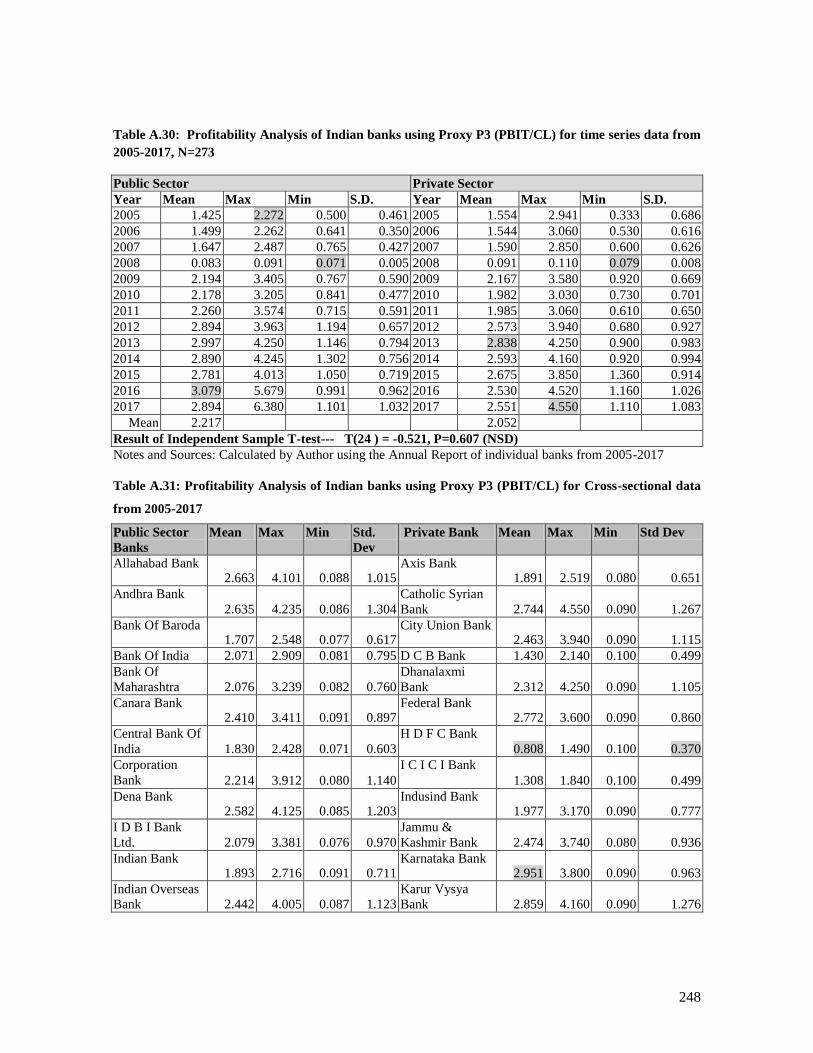
248
Table A.30: Profitability Analysis of Indian banks using Proxy P3 (PBIT/CL) for time series data from
2005-2017, N=273
Public Sector Private Sector
Year Mean Max Min S.D. Year Mean Max Min S.D.
2005 1.425 2.272 0.500 0.461 2005 1.554 2.941 0.333 0.686
2006 1.499 2.262 0.641 0.350 2006 1.544 3.060 0.530 0.616
2007 1.647 2.487 0.765 0.427 2007 1.590 2.850 0.600 0.626
2008 0.083 0.091 0.071 0.005 2008 0.091 0.110 0.079 0.008
2009 2.194 3.405 0.767 0.590 2009 2.167 3.580 0.920 0.669
2010 2.178 3.205 0.841 0.477 2010 1.982 3.030 0.730 0.701
2011 2.260 3.574 0.715 0.591 2011 1.985 3.060 0.610 0.650
2012 2.894 3.963 1.194 0.657 2012 2.573 3.940 0.680 0.927
2013 2.997 4.250 1.146 0.794 2013 2.838 4.250 0.900 0.983
2014 2.890 4.245 1.302 0.756 2014 2.593 4.160 0.920 0.994
2015 2.781 4.013 1.050 0.719 2015 2.675 3.850 1.360 0.914
2016 3.079 5.679 0.991 0.962 2016 2.530 4.520 1.160 1.026
2017 2.894 6.380 1.101 1.032 2017 2.551 4.550 1.110 1.083
Mean 2.217 2.052
Result of Independent Sample T-test--- T(24 ) = -0.521, P=0.607 (NSD)
Notes and Sources: Calculated by Author using the Annual Report of individual banks from 2005-2017
Table A.31: Profitability Analysis of Indian banks using Proxy P3 (PBIT/CL) for Cross-sectional data
from 2005-2017
Public Sector
Banks
Mean Max Min Std.
Dev
Private Bank Mean Max Min Std Dev
Allahabad Bank 2.663 4.101 0.088 1.015
Axis Bank 1.891 2.519 0.080 0.651
Andhra Bank
2.635 4.235 0.086 1.304
Catholic Syrian
Bank 2.744 4.550 0.090 1.267
Bank Of Baroda 1.707 2.548 0.077 0.617
City Union Bank 2.463 3.940 0.090 1.115
Bank Of India 2.071 2.909 0.081 0.795 D C B Bank 1.430 2.140 0.100 0.499
Bank Of
Maharashtra 2.076 3.239 0.082 0.760
Dhanalaxmi
Bank 2.312 4.250 0.090 1.105
Canara Bank 2.410 3.411 0.091 0.897
Federal Bank 2.772 3.600 0.090 0.860
Central Bank Of
India 1.830 2.428 0.071 0.603
H D F C Bank
0.808 1.490 0.100 0.370
Corporation
Bank 2.214 3.912 0.080 1.140
I C I C I Bank
1.308 1.840 0.100 0.499
Dena Bank 2.582 4.125 0.085 1.203
Indusind Bank 1.977 3.170 0.090 0.777
I D B I Bank
Ltd. 2.079 3.381 0.076 0.970
Jammu &
Kashmir Bank 2.474 3.740 0.080 0.936
Indian Bank 1.893 2.716 0.091 0.711
Karnataka Bank 2.951 3.800 0.090 0.963
Indian Overseas
Bank 2.442 4.005 0.087 1.123
Karur Vysya
Bank 2.859 4.160 0.090 1.276
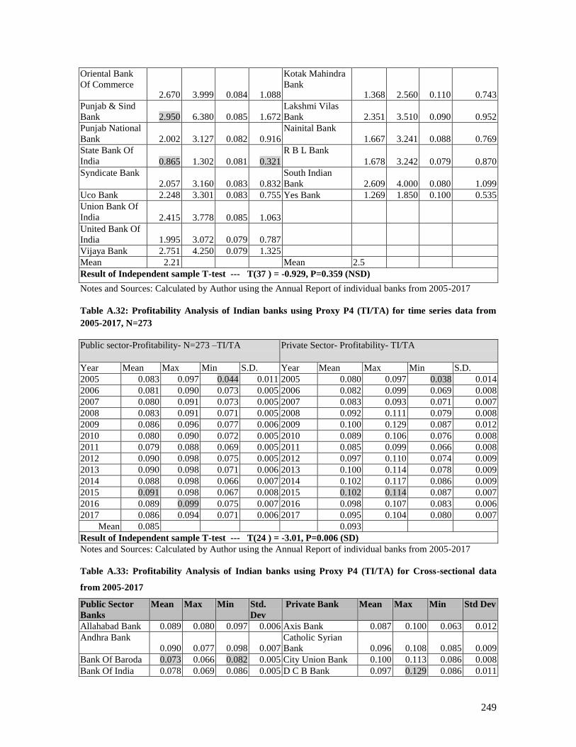
249
Oriental Bank
Of Commerce 2.670 3.999 0.084 1.088
Kotak Mahindra
Bank 1.368 2.560 0.110 0.743
Punjab & Sind
Bank 2.950 6.380 0.085 1.672
Lakshmi Vilas
Bank 2.351 3.510 0.090 0.952
Punjab National
Bank 2.002 3.127 0.082 0.916
Nainital Bank
1.667 3.241 0.088 0.769
State Bank Of
India 0.865 1.302 0.081 0.321
R B L Bank
1.678 3.242 0.079 0.870
Syndicate Bank
2.057 3.160 0.083 0.832
South Indian
Bank 2.609 4.000 0.080 1.099
Uco Bank 2.248 3.301 0.083 0.755 Yes Bank 1.269 1.850 0.100 0.535
Union Bank Of
India 2.415 3.778 0.085 1.063
United Bank Of
India 1.995 3.072 0.079 0.787
Vijaya Bank 2.751 4.250 0.079 1.325
Mean 2.21 Mean 2.5
Result of Independent sample T-test --- T(37 ) = -0.929, P=0.359 (NSD)
Notes and Sources: Calculated by Author using the Annual Report of individual banks from 2005-2017
Table A.32: Profitability Analysis of Indian banks using Proxy P4 (TI/TA) for time series data from
2005-2017, N=273
Public sector-Profitability- N=273 –TI/TA Private Sector- Profitability- TI/TA
Year Mean Max Min S.D. Year Mean Max Min S.D.
2005 0.083 0.097 0.044 0.011 2005 0.080 0.097 0.038 0.014
2006 0.081 0.090 0.073 0.005 2006 0.082 0.099 0.069 0.008
2007 0.080 0.091 0.073 0.005 2007 0.083 0.093 0.071 0.007
2008 0.083 0.091 0.071 0.005 2008 0.092 0.111 0.079 0.008
2009 0.086 0.096 0.077 0.006 2009 0.100 0.129 0.087 0.012
2010 0.080 0.090 0.072 0.005 2010 0.089 0.106 0.076 0.008
2011 0.079 0.088 0.069 0.005 2011 0.085 0.099 0.066 0.008
2012 0.090 0.098 0.075 0.005 2012 0.097 0.110 0.074 0.009
2013 0.090 0.098 0.071 0.006 2013 0.100 0.114 0.078 0.009
2014 0.088 0.098 0.066 0.007 2014 0.102 0.117 0.086 0.009
2015 0.091 0.098 0.067 0.008 2015 0.102 0.114 0.087 0.007
2016 0.089 0.099 0.075 0.007 2016 0.098 0.107 0.083 0.006
2017 0.086 0.094 0.071 0.006 2017 0.095 0.104 0.080 0.007
Mean 0.085 0.093
Result of Independent sample T-test --- T(24 ) = -3.01, P=0.006 (SD)
Notes and Sources: Calculated by Author using the Annual Report of individual banks from 2005-2017
Table A.33: Profitability Analysis of Indian banks using Proxy P4 (TI/TA) for Cross-sectional data
from 2005-2017
Public Sector
Banks
Mean Max Min Std.
Dev
Private Bank Mean Max Min Std Dev
Allahabad Bank 0.089 0.080 0.097 0.006 Axis Bank 0.087 0.100 0.063 0.012
Andhra Bank
0.090 0.077 0.098 0.007
Catholic Syrian
Bank 0.096 0.108 0.085 0.009
Bank Of Baroda 0.073 0.066 0.082 0.005 City Union Bank 0.100 0.113 0.086 0.008
Bank Of India 0.078 0.069 0.086 0.005 D C B Bank 0.097 0.129 0.086 0.011

250
Bank Of
Maharashtra 0.086 0.077 0.095 0.005
Dhanalaxmi Bank
0.090 0.105 0.074 0.011
Canara Bank 0.086 0.077 0.091 0.005 Federal Bank 0.093 0.103 0.081 0.008
Central Bank Of
India 0.084 0.071 0.099 0.008
H D F C Bank
0.094 0.108 0.074 0.010
Corporation Bank 0.085 0.072 0.098 0.008 I C I C I Bank 0.090 0.105 0.077 0.009
Dena Bank 0.085 0.079 0.09 0.003 Indusind Bank 0.100 0.116 0.080 0.011
I D B I Bank Ltd. 0.080 0.044 0.09 0.013 Jammu & Kashmir
Bank
0.084 0.101 0.067 0.010
Indian Bank 0.091 0.083 0.095 0.004 Karnataka Bank 0.093 0.101 0.080 0.007
Indian Overseas
Bank 0.090 0.075 0.098 0.006
Karur Vysya Bank
0.098 0.114 0.088 0.009
Oriental Bank Of
Commerce 0.088 0.076 0.097 0.007
Kotak Mahindra
Bank 0.105 0.127 0.086 0.012
Punjab & Sind
Bank 0.088 0.076 0.097 0.007
Lakshmi Vilas
Bank 0.095 0.112 0.079 0.010
Punjab National
Bank 0.086 0.079 0.098 0.005
Nainital Bank
0.087 0.099 0.078 0.007
State Bank Of
India 0.084 0.078 0.091 0.004
R B L Bank
0.080 0.092 0.066 0.008
Syndicate Bank 0.082 0.076 0.092 0.005 South Indian Bank 0.089 0.099 0.079 0.007
Uco Bank 0.081 0.075 0.09 0.005 Yes Bank 0.088 0.107 0.038 0.020
Union Bank Of
India 0.085 0.075 0.093 0.005
United Bank Of
India 0.087 0.076 0.098 0.008
Vijaya Bank 0.086 0.077 0.096 0.006
Mean 0.084 Mean 0.092
Result of Independent sample T-test --- T(37 ) = -4.4, P=0.000 (SD)
Notes and Sources: Calculated by Author using the Annual Report of individual banks from 2005-201
Table A.34: Leverage Analysis of Indian banks using Proxy LV1 (RE/TA) for time series data from
2005-2017, N=273
Leverage Variable (RE/TA)- of public sector
banks
Leverage Variable (RE/TA)- of public sector banks
Year
Mean Max Min S.D. Year Mean Max Min S.D.
2005 0.04 0.09 -0.06 0.03 2005 0.05 0.10 0.01 0.02
2006 0.05 0.48 0.00 0.10 2006 0.53 3.72 0.02 0.99
2007 0.05 0.07 0.02 0.02 2007 0.06 0.09 0.03 0.02
2008 0.05 0.07 0.02 0.01 2008 0.08 0.15 0.04 0.03
2009 0.05 0.08 0.02 0.01 2009 0.08 0.14 0.05 0.03
2010 0.05 0.07 0.03 0.01 2010 0.08 0.14 0.05 0.03
2011 0.05 0.07 0.03 0.01 2011 0.09 0.27 0.05 0.05
2012 0.05 0.07 0.03 0.01 2012 0.08 0.13 0.04 0.03
2013 0.05 0.07 0.04 0.01 2013 0.08 0.12 0.05 0.02
2014 0.05 0.07 0.03 0.01 2014 0.08 0.14 0.04 0.03
2015 0.05 0.08 0.04 0.01 2015 0.08 0.13 0.04 0.02
2016 0.05 0.08 0.04 0.01 2016 0.08 0.12 0.03 0.03
2017 0.05 0.08 0.04 0.01 2017 0.08 0.13 0.04 0.03
Mean 0.049 0.111
Result of Mann Whiteny U-test --- T(24 ) = -4.4, P=0.000 (SD)
Notes and Sources: Calculated by Author using the Annual Report of individual banks from 2005-2017

251
Table A.35: Leverage Analysis of Indian banks using Proxy LV1 (RE/TA) for Cross-sectional data
from 2005-2017
Public Sector
Banks
Mean Max Min Std.
Dev
Private Bank Mean Max Min Std Dev
Allahabad Bank 0.05 0.06 0.04 0.01 Axis Bank 0.09 0.15 0.04 0.03
Andhra Bank
0.05 0.06 0.04 0.01
Catholic Syrian
Bank 0.08 0.48 0.04 0.12
Bank Of Baroda 0.06 0.06 0.04 0.01 City Union Bank 0.13 0.78 0.06 0.20
Bank Of India 0.05 0.06 0.04 0.01 D C B Bank 0.08 0.28 0.03 0.06
Bank Of
Maharashtra 0.04 0.05 0.03 0.01
Dhanalaxmi Bank
0.07 0.41 0.03 0.10
Canara Bank 0.05 0.06 0.00 0.02 Federal Bank 0.08 0.12 0.04 0.02
Central Bank Of
India 0.04 0.05 0.01 0.01
H D F C Bank
0.09 0.10 0.07 0.01
Corporation Bank 0.05 0.09 0.00 0.02 I C I C I Bank 0.11 0.14 0.07 0.02
Dena Bank 0.04 0.05 0.00 0.01 Indusind Bank 0.08 0.12 0.03 0.03
I D B I Bank Ltd.
0.06 0.07 0.04 0.01
Jammu & Kashmir
Bank 0.07 0.08 0.04 0.01
Indian Bank 0.06 0.08 -0.06 0.04 Karnataka Bank 0.07 0.08 0.06 0.01
Indian Overseas
Bank 0.05 0.06 0.01 0.01
Karur Vysya Bank
0.08 0.09 0.06 0.01
Oriental Bank Of
Commerce 0.06 0.07 0.01 0.02
Kotak Mahindra
Bank 0.11 0.14 0.03 0.03
Punjab & Sind
Bank 0.08 0.48 0.01 0.12
Lakshmi Vilas
Bank 0.05 0.06 0.02 0.01
Punjab National
Bank 0.06 0.07 0.00 0.02
Nainital Bank
0.35 3.72 0.06 1.01
State Bank Of India 0.06 0.07 0.01 0.02 R B L Bank 0.15 0.58 0.03 0.14
Syndicate Bank 0.04 0.05 0.03 0.01 South Indian Bank 0.24 2.51 0.04 0.68
Uco Bank 0.04 0.07 0.02 0.01 Yes Bank 0.06 0.10 0.01 0.02
Union Bank Of
India 0.05 0.06 0.00 0.01
United Bank Of
India 0.03 0.04 -0.01 0.01
Vijaya Bank 0.04 0.05 0.01 0.01
0.050 Mean 0.110
Result of Mann Whiteny U-test --- T(37 ) = -4.8, P=0.000 (SD)
Notes and Sources: Calculated by Author using the Annual Report of individual banks from 2005-2017
Table A.36 Leverage Analysis of Indian banks using Proxy LV2 (MVE/TL) for time series data from
2005-2017, N=273
Public Sector-Efficiency- Private Sector-
Year Mean Max Min S.D. Year Mean Max Min S.D.
2005 0.07 0.15 0.01 0.03 2005 0.12 0.64 0.01 0.15
2006 0.07 0.14 0.02 0.03 2006 0.17 0.85 0.01 0.23
2007 0.09 0.69 0.01 0.14 2007 0.14 0.56 0.02 0.14
2008 0.06 0.14 0.01 0.03 2008 0.17 0.77 0.03 0.17
2009 0.03 0.07 0.01 0.02 2009 0.08 0.34 0.01 0.08
2010 0.05 0.13 0.02 0.03 2010 0.17 0.7 0.01 0.17
2011 0.07 0.14 0.04 0.03 2011 0.17 0.66 0.05 0.16
2012 0.06 0.16 0.02 0.04 2012 0.17 0.68 0.05 0.16

252
2013 0.07 0.45 0.03 0.09 2013 0.15 0.48 0.03 0.12
2014 0.03 0.08 0.01 0.01 2014 0.15 0.68 0.03 0.17
2015 0.03 0.10 0.02 0.02 2015 0.24 0.96 0.04 0.25
2016 0.02 0.07 0.01 0.01 2016 0.16 0.65 0.03 0.16
2017 0.03 0.09 0.02 0.02 2017 0.22 0.75 0.05 0.19
Mean 0.052 0.162
Result of Mann Whiteny U-test --- T(24 ) = -0.4.313, P=0.00(SD)
Notes and Sources: Calculated by Author using the Annual Report of individual banks from 2005-2017
Table A.37: Leverage Analysis of Indian banks using Proxy LV2 (MVE/TL) for Cross-sectional data
from 2005-2017
Public Sector
Banks
Mean Max Min Std.
Dev
Private Bank Mean Max Min Std
Dev
Allahabad Bank 0.04 0.07 0.01 0.02 Axis Bank 0.21 0.29 0.10 0.05
Andhra Bank
0.06 0.13 0.02 0.04
Catholic Syrian
Bank 0.05 0.08 0.01 0.02
Bank Of Baroda 0.07 0.13 0.04 0.03 City Union Bank 0.13 0.26 0.04 0.06
Bank Of India 0.05 0.08 0.01 0.02 D C B Bank 0.12 0.20 0.04 0.05
Bank Of
Maharashtra 0.03 0.05 0.02 0.01
Dhanalaxmi Bank
0.06 0.11 0.03 0.03
Canara Bank 0.10 0.69 0.02 0.18 Federal Bank 0.11 0.17 0.06 0.03
Central Bank Of
India 0.04 0.09 0.01 0.02
H D F C Bank
0.37 0.48 0.23 0.06
Corporation Bank 0.07 0.15 0.02 0.05 I C I C I Bank 0.24 0.38 0.10 0.07
Dena Bank 0.06 0.45 0.01 0.12 Indusind Bank 0.22 0.47 0.04 0.15
I D B I Bank Ltd. 0.04 0.07 0.02 0.02
Jammu & Kashmir
Bank
0.07 0.10 0.04 0.02
Indian Bank 0.06 0.10 0.03 0.02 Karnataka Bank 0.07 0.16 0.03 0.04
Indian Overseas
Bank 0.05 0.09 0.02 0.03
Karur Vysya Bank
0.11 0.16 0.06 0.03
Oriental Bank Of
Commerce 0.05 0.11 0.01 0.03
Kotak Mahindra
Bank 0.64 0.96 0.07 0.22
Punjab & Sind Bank 0.03 0.06 0.01 0.01
Lakshmi Vilas Bank 0.07 0.09 0.03 0.02
Punjab National
Bank 0.08 0.13 0.03 0.03
Nainital Bank
0.05 0.09 0.03 0.02
State Bank Of India 0.11 0.16 0.07 0.03
R B L Bank 0.12 0.65 0.01 0.19
Syndicate Bank 0.03 0.08 0.02 0.02 South Indian Bank 0.05 0.08 0.03 0.02
Uco Bank 0.03 0.05 0.01 0.01 Yes Bank 0.24 0.65 0.07 0.15
Union Bank Of
India 0.05 0.08 0.02 0.02
United Bank Of
India 0.03 0.06 0.01 0.01
Vijaya Bank 0.04 0.10 0.02 0.02
Mean 0.053 Mean 0.162
Result of Mann Whiteny U -Test T(37 ) = -3.954, P=0.000 (SD)
Notes and Sources: Calculated by Author using the Annual Report of individual banks from 2005-2017

253
Table A.38 Leverage Analysis of Indian banks using Proxy LV3 (TD/TA) for time series data from
2005-2017, N=273
Public sector-Leverage- N=273 –TD/TA Private Sector-Leverage TD/TA
Year Mean Max Min S.D. Year Mean Max Min S.D.
2005 0.881 0.972 0.900 0.018 2005 0.957 0.978 0.899 0.021
2006 0.896 0.974 0.897 0.016 2006 0.954 0.978 0.893 0.022
2007 0.919 0.973 0.923 0.012 2007 0.954 0.974 0.886 0.022
2008 0.919 0.979 0.914 0.014 2008 0.954 0.971 0.902 0.018
2009 0.915 0.979 0.917 0.012 2009 0.958 0.976 0.911 0.018
2010 0.947 0.980 0.924 0.011 2010 0.959 0.975 0.907 0.019
2011 0.969 0.982 0.914 0.013 2011 0.962 0.981 0.895 0.019
2012 0.972 0.980 0.939 0.009 2012 0.963 0.983 0.889 0.024
2013 0.972 0.982 0.940 0.009 2013 0.966 0.981 0.913 0.018
2014 0.973 0.983 0.948 0.007 2014 0.963 0.979 0.916 0.017
2015 0.971 0.980 0.935 0.009 2015 0.965 0.979 0.943 0.013
2016 0.973 0.986 0.934 0.011 2016 0.965 0.982 0.935 0.013
2017 0.973 0.988 0.944 0.009 2017 0.965 0.983 0.934 0.015
Mean 0.944 0.960
Result of Independent sample T-test --- T(24 ) = -5.38, P=0.000 (SD)
Notes and Sources: Calculated by Author using the Annual Report of individual banks from 2005-2017
Table A.39: Leverage Analysis of Indian banks using Proxy LV3 (TD/TA) for Cross-sectional data
from 2005-2017
Public Sector
Banks
Mean Max Min Std.
Dev
Private Bank Mean Max Min Std
Dev
Allahabad Bank 0.97 0.98 0.96 0.00 Axis Bank 0.98 0.97 0.96 0.01
Andhra Bank
0.97 0.98 0.94 0.01
Catholic Syrian
Bank 0.97 0.98 0.96 0.01
Bank Of Baroda 0.97 0.98 0.95 0.01 City Union Bank 0.96 0.98 0.94 0.01
Bank Of India 0.97 0.98 0.96 0.01 D C B Bank 0.96 0.97 0.94 0.01
Bank Of
Maharashtra 0.97 0.98 0.95 0.01
Dhanalaxmi Bank
0.97 0.98 0.96 0.01
Canara Bank 0.97 0.98 0.96 0.01 Federal Bank 0.97 0.98 0.96 0.01
Central Bank Of
India 0.97 0.97 0.96 0.01
H D F C Bank
0.91 0.95 0.89 0.02
Corporation Bank 0.96 0.98 0.93 0.02 I C I C I Bank 0.95 0.96 0.92 0.01
Dena Bank 0.97 0.98 0.96 0.01 Indusind Bank 0.96 0.97 0.94 0.01
I D B I Bank Ltd.
0.96 0.98 0.92 0.02
Jammu & Kashmir
Bank 0.97 0.98 0.97 0.00
Indian Bank 0.96 0.97 0.95 0.01 Karnataka Bank 0.98 0.98 0.97 0.00
Indian Overseas
Bank 0.97 0.98 0.94 0.02
Karur Vysya Bank
0.97 0.98 0.95 0.01
Oriental Bank Of
Commerce 0.97 0.98 0.96 0.01
Kotak Mahindra
Bank 0.94 0.97 0.91 0.02
Punjab & Sind
Bank 0.98 0.99 0.95 0.01
Lakshmi Vilas
Bank 0.97 0.98 0.95 0.01
Punjab National
Bank 0.96 0.98 0.92 0.02
Nainital Bank
0.96 0.98 0.94 0.01

254
State Bank Of India 0.93 0.95 0.90 0.02 R B L Bank 0.97 0.98 0.96 0.01
Syndicate Bank 0.97 0.98 0.95 0.01 South Indian Bank 0.96 0.98 0.93 0.01
Uco Bank 0.97 0.98 0.97 0.00 Yes Bank 0.95 0.98 0.92 0.02
Union Bank Of
India 0.97 0.98 0.96 0.01
United Bank Of
India 0.97 0.98 0.95 0.01
Vijaya Bank 0.97 0.98 0.96 0.01
Mean 0.943 Mean 0.960
Result of Independent sample T-test --- T(37 ) = -1.4, P=0.000 (SD)
Notes and Sources: Calculated by Author using the Annual Report of individual banks from 2005-2017
Table A.40: Result of Altman Z-score of 21 public banks for 2005-2017
Sr.
No Public Banks 2005 2006 2007 2008 2009 2010 2011 2012 2013 2014 2015 2016 2017 Avg Result
1 Allahabad Bank
(2005) 1.07 1.34 1.02 1.00 1.09 1.12 1.07 1.23 1.19 1.11 1.19 1.29 1.27 1.15 Grey
2 Andhra Bank 1.22 1.25 1.11 1.30 1.20 1.52 1.47 1.37 1.21 1.31 1.53 1.39 1.52 1.34 Grey
3 Bank Of
Baroda 1.16 1.33 1.07 1.60 1.52 1.47 1.97 1.98 1.73 1.91 1.31 1.52 1.64 1.55 Grey
4 Bank Of India 0.86 1.20 1.34 1.24 1.33 1.41 1.23 1.36 1.36 1.29 1.33 1.27 1.43 1.28 Grey
5 Bank Of
Maharashtra 1.03 1.03 0.99 1.03 0.98 1.17 0.85 1.02 1.19 1.04 1.22 1.30 1.71 1.12 Grey
6 Canara Bank 1.06 1.18 1.75 1.24 1.25 1.24 1.37 1.34 1.32 1.35 1.40 1.50 1.51 1.35 Grey
7 Central Bank
Of India 1.19 0.99 1.15 1.11 0.98 1.17 0.98 0.98 1.00 0.87 1.03 1.08 1.92 1.11 Grey
8 Corporation
Bank 1.27 1.31 1.11 1.39 1.51 1.12 0.73 1.20 1.24 1.19 1.11 1.23 1.48 1.22 Grey
9 Dena Bank 1.06 1.28 1.57 1.62 1.96 1.28 1.20 1.18 1.86 1.15 1.43 1.18 1.29 1.39 Grey
10 I D B I Bank 0.61 1.07 1.06 1.07 1.04 0.81 1.19 1.19 1.06 1.06 1.21 1.34 1.24 1.07 Distres
s
11 Indian Bank 0.59 1.26 1.14 1.44 1.27 1.28 1.17 1.16 1.22 1.14 1.33 1.29 1.20 1.19 Grey
12 Indian Overseas
Bank 1.20 1.03 1.03 1.10 1.39 1.25 1.54 1.32 1.27 1.28 1.43 1.30 1.37 1.27 Grey
13 Oriental Bank
Of Commerce 1.66 1.32 1.25 1.30 1.40 1.34 1.15 1.14 1.08 1.27 1.29 1.35 1.67 1.32 Grey
14 Punjab & Sind
Bank 1.11 1.29 1.52 0.87 1.01 0.82 0.80 0.94 1.08 1.10 1.18 1.29 1.29 1.10
Distres
s
15 Punjab National
Bank 0.90 1.73 1.37 1.28 1.25 1.27 1.19 1.28 1.16 1.27 1.20 1.43 1.69 1.31 Grey
16 State Bank Of
India 1.28 1.15 0.88 1.09 1.25 1.11 1.41 1.24 1.23 1.05 1.45 1.37 1.38 1.22 Grey
17 Syndicate Bank 0.77 1.02 1.55 1.33 1.33 0.87 0.99 1.10 1.08 0.77 0.97 1.10 1.03 1.07 Grey
18 Uco Bank 1.35 0.80 1.01 1.14 1.27 0.99 1.52 1.28 1.18 1.00 1.41 1.14 1.13 1.17 Grey
19 Union Bank Of
India 1.16 0.92 0.98 1.20 1.28 1.16 1.22 1.03 0.99 1.08 1.16 1.23 1.12 1.04
Distres
s
20 United Bank Of
India 1.10 1.07 1.23 1.33 1.32 1.11 1.18 1.23 1.28 1.32 1.32 1.37 1.64 1.18 Grey
21 Vijaya Bank 0.94 1.13 1.45 1.77 2.14 1.03 1.08 1.21 1.11 1.31 1.38 1.67 1.46 1.25 Grey
Source: Authors Calculations based on the data from CMIE

255
Table A.41 Result of Altman Z- score of 18 Private Banks for 2005-2017
Sr.
No.
Private
Banks 2005 2006 2007 2008 2009 2010 2011 2012 2013 2014 2015 2016 2017 Avg Mean
1 Axis Bank 1.46 0.97 1.38 1.67 1.47 1.51 1.35 1.28 1.33 1.37 2.00 2.18 2.45 1.57 Grey
2 Catholic
Syrian Bank 1.93 1.41 1.64 1.75 2.18 1.62 1.41 1.64 1.71 1.23 1.46 1.44 1.66 1.62 Grey
3 City Union
Bank 1.20 1.05 1.11 1.53 1.45 1.48 1.44 1.35 1.55 1.58 1.84 1.67 1.74 1.46 Grey
4 D C B Bank 0.93 0.92 1.24 1.48 1.74 1.09 0.74 0.72 0.81 0.97 1.65 1.34 1.74 1.18 Grey
5 Dhanlaxmi
Bank 1.31 1.17 1.22 1.68 1.65 1.27 1.16 1.21 1.42 1.33 1.98 1.67 1.72 1.44 Grey
6 Federal Bank 2.02 1.54 1.22 1.76 1.63 1.23 1.72 1.53 1.46 1.56 1.56 1.55 1.83 1.58 Grey
7 H D F C Bank 0.77 0.94 1.04 1.80 1.27 1.54 1.46 1.25 1.47 1.65 1.45 1.90 1.58 1.40 Grey
8 I C I C I Bank 1.00 1.06 1.23 1.62 1.62 1.89 1.61 1.57 1.72 1.60 1.66 1.78 1.84 1.55 Grey
9 Indusind
Bank 1.09 1.25 1.40 1.38 1.59 1.39 1.79 1.27 1.60 1.34 1.41 1.58 1.87 1.46 Grey
10 Jammu &
Kashmir Bank 1.39 1.42 1.76 2.34 1.97 1.73 1.25 1.24 1.27 1.06 1.11 1.32 1.50 1.49 Grey
11 Karnataka
Bank 2.43 1.74 1.15 1.45 1.28 1.19 1.14 1.14 1.16 1.08 1.50 1.48 1.38 1.39 Grey
12 Karur Vysya
Bank 1.31 1.44 1.12 1.20 1.42 1.21 1.26 1.46 1.23 1.08 1.22 1.34 1.39 1.28 Grey
13
Kotak
Mahindra
Bank
1.11 1.15 0.32 1.60 1.25 1.53 1.46 1.64 1.02 1.86 2.13 1.85 2.06 1.46 Grey
14 Lakshmi
Vilas Bank 1.71 1.30 1.83 1.41 1.44 1.26 0.91 1.24 1.25 1.24 1.20 1.14 1.05 1.31 Grey
15 Nainital Bank 1.95 1.96 2.10 3.48 2.56 2.56 2.96 2.32 3.04 2.62 2.90 3.50 2.51 2.65 Safe
16 R B L Bank 1.50 1.54 1.93 3.20 2.78 1.66 1.84 1.55 1.26 1.26 1.33 1.10 1.69 1.74 Grey
17 South Indian
Bank 0.93 1.26 1.37 1.26 1.12 1.24 1.32 1.17 1.24 1.21 1.55 1.51 1.38 1.27 Grey
18 Yes Bank 0.12 1.23 1.60 1.09 1.17 1.09 0.97 0.94 1.11 1.48 1.31 1.7 1.06 Distress
Source: Authors calculations based on data from CMIE
Table A.42 Result of Altman Z-score of five NWB from 2005-2013
Sr.
No. Banks 2005 2006 2007 2008 2009 2010 2011 2012 2013 Avg Result
1 Bank Of Punjab Ltd.
[Merged] 1.42 ---- ----- ----- ---- ---- ----- ----- ---- 1.42 Grey
2 Bank Of Rajasthan
Ltd. [Merged] 2.04 2.50 1.50 1.71 1.24 0.84 ---- ----- ----- 1.52 Grey
3 Bharat Overseas
Bank Ltd. [Merged] 1.29 1.49 ---- ----- ----- ---- ---- ----- ----- 1.39 Grey
4 Centurion Bank Of
Punjab Ltd. [Merged] 1.15 1.38 0.57 ---- ----- ----- ---- ---- ----- 1.03 Distress
5 I N G Vysya Bank
Ltd. [Merged] 0.90 0.81 0.89 1.49 1.10 1.21 1.09 1.23 1.26 1.31 Grey
Source: Authors calculations based on data from CMIE
Table A.43: Result of Springate Model of 21 public banks for 2005-2017
Sr.
No. Bank 2005 2006 2007 2008 2009 2010 2011 2012 2013 2014 2015 2016 2017 Avg Result
1 Allahabad
Bank 1.82 1.50 1.97 2.00 1.99 2.03 2.04 2.99 3.08 2.60 2.23 2.49 2.31 2.23 Safe

256
2 Andhra Bank 1.21 0.95 1.47 1.57 2.00 2.11 2.40 2.83 3.15 3.20 2.71 2.90 2.16 2.20 Safe
3 Bank Of
Baroda 1.15 1.21 1.31 1.44 1.51 1.64 1.90 2.15 1.94 1.83 1.69 1.71 1.77 1.64 Safe
4 Bank Of India 1.31 1.31 1.36 1.63 2.09 1.77 1.37 1.92 2.31 1.95 2.20 2.26 2.21 1.82 Safe
5 Bank Of
Maharashtra 1.53 1.47 1.43 1.25 1.64 1.75 1.49 1.77 2.12 2.25 2.00 2.53 1.99 1.79 Safe
6 Canara Bank 1.36 1.33 1.65 1.65 2.07 2.21 2.35 2.64 2.35 2.38 2.24 2.33 2.22 2.06 Safe
7 Central Bank
Of India 1.32 1.44 1.45 1.31 1.53 1.82 1.61 1.78 1.92 1.61 1.52 1.68 2.08 1.62 Safe
8 Corporation
Bank 0.95 1.07 1.02 1.14 1.76 1.59 1.97 2.26 2.45 2.56 2.57 2.98 2.05 1.87 Safe
9 Dena Bank 1.34 1.54 1.44 1.56 1.73 1.57 2.70 2.66 3.13 2.79 2.57 2.81 2.58 2.19 Safe
10 I D B I Bank 0.48 1.44 1.36 1.52 1.62 1.60 2.19 2.60 2.30 2.20 2.28 2.16 1.75 1.81 Safe
11 Indian Bank 1.13 1.34 1.23 1.64 1.59 1.62 1.73 1.89 1.76 1.86 2.04 2.16 2.01 1.69 Safe
12 Indian
Overseas Bank 1.42 1.23 1.01 1.11 2.31 1.98 1.89 2.35 2.64 2.66 3.07 2.46 2.46 2.05 Safe
13 Oriental Bank
Of Commerce 1.90 1.53 1.86 1.57 1.88 2.00 1.67 2.64 2.95 2.59 2.42 2.91 3.10 2.23 Safe
14 Punjab & Sind
Bank 1.15 1.46 1.95 2.34 2.57 2.38 1.76 2.27 2.11 2.39 2.65 4.14 4.60 2.44 Safe
15 Punjab
National Bank 0.76 1.17 1.41 1.33 1.58 1.65 1.68 2.05 2.09 2.16 2.04 2.41 2.51 1.76 Safe
16 State Bank Of
India 0.79 0.74 0.79 0.78 0.85 0.86 0.83 1.12 1.09 1.16 1.07 1.02 1.08 0.94 Safe
17 Syndicate Bank 1.06 1.13 1.52 1.69 1.88 1.76 1.81 2.26 1.90 1.56 1.95 2.24 2.42 1.78 Safe
18 Uco Bank 1.52 1.76 1.77 2.14 2.57 2.02 1.74 2.23 2.12 2.01 2.01 1.98 1.83 1.98 Safe
19 Union Bank Of
India 1.36 1.21 1.47 1.78 1.95 1.90 1.58 2.11 2.44 2.67 2.50 2.87 2.64 2.04 Safe
20 United Bank
Of India 1.34 1.34 1.38 1.39 1.41 1.59 1.69 2.40 2.22 2.03 1.91 2.05 2.28 1.77 Safe
21 Vijaya Bank 1.57 1.52 1.47 1.60 1.97 1.50 2.04 2.91 3.16 3.20 3.07 3.04 2.86 2.30 Safe
Source: Authors calculations based on data from CMIE
Table A.44: Result of Springate Model of 18 private banks for 2005-2017
Sr.
No.
Bank (ZM –
Score) 2005 2006 2007 2008 2009 2010 2011 2012 2013 2014 2015 2016 2017 Avg Result
1 Axis Bank 1.52 1.09 1.52 1.46 1.99 1.65 1.54 1.99 1.99 1.82 1.90 1.70 1.49 1.67 Safe
2 Catholic
Syrian Bank 2.21 1.55 1.54 1.57 1.95 1.82 1.94 2.34 2.71 3.00 2.84 3.40 3.45 2.33 Safe
3 City Union
Bank 1.66 1.13 1.25 1.51 1.98 1.94 2.00 3.00 2.94 2.91 2.35 2.46 2.32 2.11 Safe
4 D C B Bank 0.97 1.22 1.33 1.59 1.92 1.33 1.14 1.31 1.57 1.39 1.36 1.06 1.18 1.34 Safe
5 Dhanlaxmi
Bank 1.25 1.31 1.49 1.50 1.94 1.60 2.09 2.05 3.23 1.83 2.77 1.95 2.82 1.99 Safe
6 Federal Bank 2.47 2.04 2.10 1.67 2.50 2.23 2.15 2.44 2.42 2.60 2.87 2.47 2.46 2.34 Safe
7 H D F C Bank
0.52 0.55 0.67 0.87 0.95 0.80 0.70 0.73 0.91 0.98 1.25 1.31 0.84 0.85 Distres
s
8 I C I C I Bank 0.77 0.90 1.17 1.37 1.63 1.59 1.43 1.02 1.17 1.21 1.40 1.44 1.57 1.28 Safe
9 Indusind Bank 1.63 1.68 1.67 1.76 1.92 1.64 1.72 2.21 2.45 2.30 1.31 1.40 1.41 1.78 Safe
10 Jammu &
Kashmir Bank 1.63 1.59 1.86 1.94 2.24 2.07 2.11 2.19 2.74 2.55 2.81 2.15 1.82 2.13 Safe
11 Karnataka 1.99 2.46 2.26 2.16 2.76 2.35 2.34 2.71 2.87 2.36 2.52 2.83 2.60 2.48 Safe

257
Bank
12 Karur Vysya
Bank 1.36 1.53 1.60 1.75 2.08 2.29 1.96 2.88 3.06 3.11 2.92 3.08 3.03 2.36 Safe
13
Kotak
Mahindra
Bank
0.64 0.63 0.63 0.84 0.97 0.90 1.00 1.71 2.00 1.89 1.53 1.37 1.58 1.21 Safe
14 Lakshmi Vilas
Bank 1.62 1.39 1.67 1.40 1.58 2.03 1.58 2.30 2.45 2.62 2.32 2.45 2.64 2.00 Safe
15 Nainital Bank 1.46 1.06 1.34 1.79 1.69 1.69 1.68 2.38 1.99 1.62 2.82 1.84 1.84 1.79 Safe
16 R B L Bank 1.32 1.21 0.98 1.90 2.11 0.93 1.10 2.48 2.18 1.50 1.81 1.60 1.66 1.60 Safe
17 South Indian
Bank 1.45 1.39 1.61 1.70 2.13 2.08 1.90 2.33 2.58 2.57 2.79 3.02 3.03 2.20 Safe
18 Yes Bank 0.24 1.40 0.77 1.71 1.34 1.22 1.33 1.03 1.31 1.39 1.45 1.44 1.33 1.23 Safe
Source: Authors calculations based on data from CMIE
Table A.45: Result of Springate Model NWB banks from 2005-2014
Sr.
No Bank (ZM –Score) 2005 2006 2007 2008 2009 2010 2011 Avg Result
1 Bank Of Punjab Ltd. [Merged] 1.42 ---- ----- ----- ---- ---- ----- 1.42 Safe
2 Bank Of Rajasthan Ltd. [Merged] 1.20 1.19 1.25 1.30 1.40 0.93 1.14 Safe
3 Bharat Overseas Bank Ltd. [Merged] 1.19 1.24 ---- ----- ----- ---- 1.81 Safe
4 Centurion Bank Of Punjab Ltd.
[Merged] 1.04 0.99 0.73 ---- ----- ----- ---- 0.92 Safe
5 I N G Vysya Bank Ltd. [Merged] 0.97 0.97 0.86 0.94 0.98 1.01 1.08 1.14 Safe
Source: Authors calculations based on data from CMIE
TableA.46: Result of Zmijewski model for 21 public banks from 2005-2017
Sr.
No. Bank 2005 2006 2007 2008 2009 2010 2011 2012 2013 2014 2015 2016 2017 Avg Result
1 Allahabad Bank 1.82 1.50 1.97 2.00 1.99 2.03 2.04 2.99 3.08 2.60 2.23 2.49 2.31 2.23 Safe
2 Andhra Bank 1.21 0.95 1.47 1.57 2.00 2.11 2.40 2.83 3.15 3.20 2.71 2.90 2.16 2.20 Safe
3 Bank Of Baroda 1.15 1.21 1.31 1.44 1.51 1.64 1.90 2.15 1.94 1.83 1.69 1.71 1.77 1.64 Safe
4 Bank Of India 1.31 1.31 1.36 1.63 2.09 1.77 1.37 1.92 2.31 1.95 2.20 2.26 2.21 1.82 Safe
5 Bank Of
Maharashtra 1.53 1.47 1.43 1.25 1.64 1.75 1.49 1.77 2.12 2.25 2.00 2.53 1.99 1.79 Safe
6 Canara Bank 1.36 1.33 1.65 1.65 2.07 2.21 2.35 2.64 2.35 2.38 2.24 2.33 2.22 2.06 Safe
7 Central Bank Of
India 1.32 1.44 1.45 1.31 1.53 1.82 1.61 1.78 1.92 1.61 1.52 1.68 2.08 1.62 Safe
8 Corporation
Bank 0.95 1.07 1.02 1.14 1.76 1.59 1.97 2.26 2.45 2.56 2.57 2.98 2.05 1.87 Safe
9 Dena Bank 1.34 1.54 1.44 1.56 1.73 1.57 2.70 2.66 3.13 2.79 2.57 2.81 2.58 2.19 Safe
10 I D B I Bank
Ltd. 0.48 1.44 1.36 1.52 1.62 1.60 2.19 2.60 2.30 2.20 2.28 2.16 1.75 1.81 Safe
11 Indian Bank 1.13 1.34 1.23 1.64 1.59 1.62 1.73 1.89 1.76 1.86 2.04 2.16 2.01 1.69 Safe
12 Indian Overseas
Bank 1.42 1.23 1.01 1.11 2.31 1.98 1.89 2.35 2.64 2.66 3.07 2.46 2.46 2.05 Safe
13 Oriental Bank Of
Commerce 1.90 1.53 1.86 1.57 1.88 2.00 1.67 2.64 2.95 2.59 2.42 2.91 3.10 2.23 Safe
14 Punjab & Sind
Bank 1.15 1.46 1.95 2.34 2.57 2.38 1.76 2.27 2.11 2.39 2.65 4.14 4.60 2.44 Safe
15 Punjab National
Bank 0.76 1.17 1.41 1.33 1.58 1.65 1.68 2.05 2.09 2.16 2.04 2.41 2.51 1.76 Safe

258
16 State Bank Of
India 0.79 0.74 0.79 0.78 0.85 0.86 0.83 1.12 1.09 1.16 1.07 1.02 1.08 0.94 Safe
17 Syndicate Bank 1.06 1.13 1.52 1.69 1.88 1.76 1.81 2.26 1.90 1.56 1.95 2.24 2.42 1.78 Safe
18 Uco Bank 1.52 1.76 1.77 2.14 2.57 2.02 1.74 2.23 2.12 2.01 2.01 1.98 1.83 1.98 Safe
19 Union Bank Of
India 1.36 1.21 1.47 1.78 1.95 1.90 1.58 2.11 2.44 2.67 2.50 2.87 2.64 2.04 Safe
20 United Bank Of
India 1.34 1.34 1.38 1.39 1.41 1.59 1.69 2.40 2.22 2.03 1.91 2.05 2.28 1.77 Safe
21 Vijaya Bank 1.57 1.52 1.47 1.60 1.97 1.50 2.04 2.91 3.16 3.20 3.07 3.04 2.86 2.30 Safe
Source: Authors calculations based on data from CMIE
TableA.47: Result of Zmijewski model for18 Private banks from 2005-2017
Sr,
No
Bank (ZM –
Score) 2005 2006 2007 2008 2009 2010 2011 2012 2013 2014 2015 2016 2017 Avg Result
1 Axis Bank 1.23 1.10 1.19 1.16 1.18 1.16 1.16 1.17 1.16 1.13 1.15 1.13 1.13 1.16 Safe
2 Catholic
Syrian Bank 1.26 1.24 1.19 1.16 1.23 1.26 1.28 1.27 1.28 1.29 1.31 1.37 1.34 1.27 Safe
3 City Union
Bank 1.13 1.00 1.05 1.07 1.14 1.15 1.16 1.22 1.22 1.21 1.16 1.19 1.18 1.14 Safe
4 D C B Bank 1.27 1.27 1.20 1.18 1.24 1.24 1.15 1.14 1.17 1.10 1.08 0.99 1.07 1.16 Safe
5 Dhanlaxmi
Bank 1.21 1.18 1.19 1.15 1.21 1.24 1.31 1.29 1.31 1.31 1.38 1.33 1.31 1.26 Safe
6 Federal Bank 1.29 1.23 1.22 1.13 1.21 1.19 1.21 1.20 1.21 1.22 1.24 1.27 1.27 1.22 Safe
7 H D F C
Bank 0.77 0.74 0.70 0.80 0.85 0.82 0.75 0.70 0.83 0.85 1.02 1.05 0.96 0.83 Safe
8 I C I C I
Bank 0.91 1.02 1.06 1.05 1.09 1.12 1.13 0.96 1.00 1.00 1.05 1.08 1.10 1.04 Safe
9 Indusind
Bank 1.13 1.22 1.19 1.18 1.18 1.15 1.15 1.17 1.18 1.16 1.01 1.05 1.05 1.14 Safe
10 Jammu & K
Bank 1.23 1.21 1.22 1.19 1.22 1.21 1.22 1.20 1.22 1.21 1.25 1.24 1.33 1.23 Safe
11 Karnataka
Bank 1.19 1.25 1.22 1.19 1.23 1.25 1.26 1.26 1.24 1.23 1.23 1.26 1.26 1.24 Safe
12 Karur Vysya
Bank 1.09 1.11 1.12 1.15 1.16 1.20 1.17 1.23 1.24 1.24 1.23 1.25 1.25 1.19 Safe
13
Kotak
Mahindra
Bank
0.93 0.85 0.93 0.87 0.88 0.90 0.99 1.11 1.14 1.11 1.07 1.10 1.11 1.00 Safe
14 Lakshmi
Vilas Bank 1.21 1.18 1.21 1.11 1.15 1.22 1.16 1.21 1.21 1.25 1.22 1.23 1.25 1.20 Safe
15 Nainital Bank 1.16 1.05 1.10 1.10 1.10 1.12 1.13 1.21 1.13 1.11 1.28 1.16 1.22 1.14 Safe
16 R B L Bank 1.22 1.15 1.08 1.21 1.17 0.97 1.23 1.29 1.26 1.17 1.21 1.19 1.16 1.18 Safe
17 South Indian
Bank 1.18 1.18 1.18 1.18 1.21 1.22 1.21 1.21 1.23 1.23 1.27 1.29 1.29 1.22 Safe
18 Yes Bank 1.29 1.19 0.98 1.13 1.00 1.07 1.10 0.91 1.03 1.00 1.05 1,06 1.03 1.07 Safe
Source: Authors calculations based on data from CMIE
Table A.48: Results of Zmijewski Model for NWB from 2005-2014
Sr,
No Bank (ZM –Score) 2005 2006 2007 2008 2009 2010 2011 2012 2013 2014 Avg Result
1 Bank Of Punjab (M) 1.23 ---- ----- ----- ---- ---- ----- ----- ---- ---- 1.23 safe
2 Bank Of Rajasth. (M) 1.17 1.18 1.14 1.14 1.15 1.12 ---- ----- ----- ---- 1.15 safe

259
3 Bharat Oves Bank Ltd.
(M) 1.13 1.18 ---- ----- ----- ---- ---- ----- ----- ---- 1.15 safe
4 Centurion Bank Of
Punjab Ltd. [Merged] 1.04 1.01 0.95 ---- ----- ----- ---- ---- ----- ----- 1.00 safe
5 I N G Vysya Bank
Ltd. (M) 1.12 1.12 1.01 0.98 1.01 1.04 1.07 1.11 1.11 1.13 1.07 safe
Source: Authors calculations based on data from CMIE
TableA.49: Result of Grover model of 21 Public Sector banks from 2005-2017
Sr.
No. Bank 2005 2006 2007 2008 2009 2010 2011 2012 2013 2014 2015 2016 2017 Avg Result
1 Allahabad
Bank 0.37 0.41 0.38 0.36 0.40 0.39 0.36 0.42 0.43 0.42 0.44 0.47 0.45 0.41 Safe
2 Andhra Bank 0.39 0.37 0.38 0.43 0.42 0.48 0.46 0.46 0.43 0.47 0.44 0.45 0.49 0.44 Safe
3 Bank Of
Baroda 0.38 0.40 0.46 0.49 0.48 0.44 0.55 0.56 0.52 0.56 0.59 0.66 0.71 0.52 Safe
4 Bank Of India 0.32 0.39 0.38 0.40 0.43 0.45 0.39 0.45 0.46 0.44 0.45 0.52 0.53 0.43 Safe
5 Bank Of
Maharashtra 0.39 0.39 0.38 0.38 0.38 0.41 0.33 0.38 0.43 0.41 0.44 0.47 0.58 0.41 Safe
6 Canara Bank 0.36 0.38 0.40 0.43 0.43 0.41 0.43 0.45 0.46 0.46 0.48 0.52 0.50 0.44 Safe
7 Central Bank
Of India 0.43 0.37 0.42 0.39 0.38 0.41 0.36 0.38 0.37 0.37 0.38 0.42 0.61 0.41 Safe
8 Corporation
Bank 0.36 0.37 0.37 0.44 0.49 0.37 0.27 0.43 0.43 0.45 0.43 0.47 0.51 0.41 Safe
9 Dena Bank 0.40 0.44 0.45 0.52 0.61 0.43 0.40 0.42 0.48 0.42 0.55 0.49 0.56 0.47 Safe
10 I D B I Bank 0.21 0.41 0.39 0.37 0.38 0.33 0.41 0.42 0.39 0.39 0.49 0.62 0.51 0.41 Safe
11 Indian Bank 0.32 0.41 0.41 0.44 0.41 0.40 0.38 0.39 0.41 0.40 0.44 0.43 0.39 0.40 Safe
12 Indian Oves
Bank 0.41 0.35 0.37 0.38 0.47 0.43 0.49 0.46 0.45 0.46 0.51 0.49 0.51 0.45 Safe
13 Oriental Bank
Of Commerce 0.48 0.38 0.43 0.43 0.47 0.44 0.38 0.41 0.40 0.45 0.46 0.48 0.56 0.44 Safe
14 Punjab & Sind
Bank 0.43 0.42 0.51 0.31 0.37 0.31 0.31 0.38 0.41 0.42 0.44 0.46 0.46 0.40 Safe
15 Punjab
National Bank 0.29 0.50 0.45 0.40 0.42 0.39 0.38 0.41 0.40 0.43 0.41 0.50 0.54 0.42 Safe
16 State Bank Of
India 0.42 0.37 0.33 0.33 0.40 0.35 0.42 0.39 0.38 0.35 0.45 0.44 0.42 0.39 Safe
17 Syndicate Bank 0.30 0.34 0.49 0.46 0.46 0.34 0.36 0.41 0.39 0.31 0.37 0.43 0.40 0.39 Safe
18 Uco Bank 0.46 0.32 0.40 0.43 0.46 0.38 0.50 0.47 0.45 0.38 0.49 0.45 0.43 0.43 Safe
19 Union Bank Of
India 0.39 0.32 0.38 0.40 0.43 0.38 0.39 0.37 0.37 0.40 0.43 0.44 0.41 0.39 Safe
20 United Bank Of
India 0.43 0.39 0.46 0.45 0.45 0.39 0.41 0.43 0.46 0.50 0.48 0.50 0.55 0.45 Safe
21 Vijaya Bank 0.33 0.40 0.54 0.56 0.69 0.39 0.38 0.45 0.42 0.47 0.50 0.56 0.50 0.48 Safe
Source: Authors calculations based on data from CMIE
Table A.50: Result of Grover model for 18 Private Banks from 2005-2017
Sr.
No. Bank 2005 2006 2007 2008 2009 2010 2011 2012 2013 2014 2015 2016 2017 Avg Result
1 Axis Bank 0.41 0.29 0.36 0.43 0.45 0.39 0.35 0.36 0.37 0.38 0.39 0.38 0.43 0.38 Safe
2 Catholic Syrian 0.62 0.45 0.56 0.54 0.65 0.53 0.44 0.53 0.55 0.45 1.04 0.50 0.53 0.57 Safe
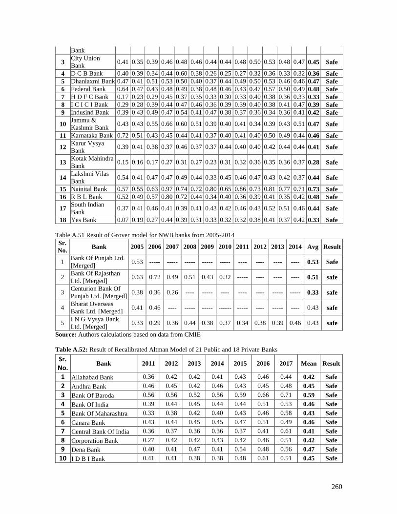
260
Bank
3 City Union
Bank 0.41 0.35 0.39 0.46 0.48 0.46 0.44 0.44 0.48 0.50 0.53 0.48 0.47 0.45 Safe
4 D C B Bank 0.40 0.39 0.34 0.44 0.60 0.38 0.26 0.25 0.27 0.32 0.36 0.33 0.32 0.36 Safe
5 Dhanlaxmi Bank 0.47 0.41 0.51 0.53 0.50 0.40 0.37 0.44 0.49 0.50 0.53 0.46 0.46 0.47 Safe
6 Federal Bank 0.64 0.47 0.43 0.48 0.49 0.38 0.48 0.46 0.43 0.47 0.57 0.50 0.49 0.48 Safe
7 H D F C Bank 0.17 0.23 0.29 0.45 0.37 0.35 0.33 0.30 0.33 0.40 0.38 0.36 0.33 0.33 Safe
8 I C I C I Bank 0.29 0.28 0.39 0.44 0.47 0.46 0.36 0.39 0.39 0.40 0.38 0.41 0.47 0.39 Safe
9 Indusind Bank 0.39 0.43 0.49 0.47 0.54 0.41 0.47 0.38 0.37 0.36 0.34 0.36 0.41 0.42 Safe
10 Jammu &
Kashmir Bank 0.43 0.43 0.55 0.66 0.60 0.51 0.39 0.40 0.41 0.34 0.39 0.43 0.51 0.47 Safe
11 Karnataka Bank 0.72 0.51 0.43 0.45 0.44 0.41 0.37 0.40 0.41 0.40 0.50 0.49 0.44 0.46 Safe
12 Karur Vysya
Bank 0.39 0.41 0.38 0.37 0.46 0.37 0.37 0.44 0.40 0.40 0.42 0.44 0.44 0.41 Safe
13 Kotak Mahindra
Bank 0.15 0.16 0.17 0.27 0.31 0.27 0.23 0.31 0.32 0.36 0.35 0.36 0.37 0.28 Safe
14 Lakshmi Vilas
Bank 0.54 0.41 0.47 0.47 0.49 0.44 0.33 0.45 0.46 0.47 0.43 0.42 0.37 0.44 Safe
15 Nainital Bank 0.57 0.55 0.63 0.97 0.74 0.72 0.80 0.65 0.86 0.73 0.81 0.77 0.71 0.73 Safe
16 R B L Bank 0.52 0.49 0.57 0.80 0.72 0.44 0.34 0.40 0.36 0.39 0.41 0.35 0.42 0.48 Safe
17 South Indian
Bank 0.37 0.41 0.46 0.41 0.39 0.41 0.43 0.42 0.46 0.43 0.52 0.51 0.46 0.44 Safe
18 Yes Bank 0.07 0.19 0.27 0.44 0.39 0.31 0.33 0.32 0.32 0.38 0.41 0.37 0.42 0.33 Safe
Table A.51 Result of Grover model for NWB banks from 2005-2014
Sr.
No. Bank 2005 2006 2007 2008 2009 2010 2011 2012 2013 2014 Avg Result
1 Bank Of Punjab Ltd.
[Merged] 0.53 ----- ----- ----- ----- ----- ---- ---- ---- ---- 0.53 Safe
2 Bank Of Rajasthan
Ltd. [Merged] 0.63 0.72 0.49 0.51 0.43 0.32 ----- ---- ---- ---- 0.51 safe
3 Centurion Bank Of
Punjab Ltd. [Merged] 0.38 0.36 0.26 ---- ----- ---- ---- ---- ----- ----- 0.33 safe
4 Bharat Overseas
Bank Ltd. [Merged] 0.41 0.46 ---- ----- ----- ------ ----- ---- ----- ---- 0.43 safe
5 I N G Vysya Bank
Ltd. [Merged] 0.33 0.29 0.36 0.44 0.38 0.37 0.34 0.38 0.39 0.46 0.43 safe
Source: Authors calculations based on data from CMIE
Table A.52: Result of Recalibrated Altman Model of 21 Public and 18 Private Banks
Sr. No.
Bank 2011 2012 2013 2014 2015 2016 2017 Mean Result
1 Allahabad Bank 0.36 0.42 0.42 0.41 0.43 0.46 0.44 0.42 Safe
2 Andhra Bank 0.46 0.45 0.42 0.46 0.43 0.45 0.48 0.45 Safe
3 Bank Of Baroda 0.56 0.56 0.52 0.56 0.59 0.66 0.71 0.59 Safe
4 Bank Of India 0.39 0.44 0.45 0.44 0.44 0.51 0.53 0.46 Safe
5 Bank Of Maharashtra 0.33 0.38 0.42 0.40 0.43 0.46 0.58 0.43 Safe
6 Canara Bank 0.43 0.44 0.45 0.45 0.47 0.51 0.49 0.46 Safe
7 Central Bank Of India 0.36 0.37 0.36 0.36 0.37 0.41 0.61 0.41 Safe
8 Corporation Bank 0.27 0.42 0.42 0.43 0.42 0.46 0.51 0.42 Safe
9 Dena Bank 0.40 0.41 0.47 0.41 0.54 0.48 0.56 0.47 Safe
10 I D B I Bank 0.41 0.41 0.38 0.38 0.48 0.61 0.51 0.45 Safe

261
11 Indian Bank 0.37 0.38 0.40 0.39 0.43 0.43 0.39 0.40 Safe
12 Indian Overseas Bank 0.49 0.46 0.44 0.45 0.50 0.48 0.50 0.47 Safe
13 Oriental Bank Of
Commerce 0.37 0.40 0.39 0.44 0.45 0.47 0.56 0.44 Safe
14 Punjab & Sind Bank 0.31 0.37 0.40 0.41 0.43 0.45 0.45 0.40 Safe
15 Punjab National Bank 0.37 0.40 0.39 0.42 0.40 0.49 0.54 0.43 Safe
16 State Bank Of India 0.42 0.38 0.38 0.35 0.44 0.44 0.42 0.40 Safe
17 Syndicate Bank 0.35 0.40 0.38 0.30 0.36 0.42 0.39 0.37 Safe
18 Uco Bank 0.50 0.46 0.44 0.37 0.48 0.44 0.42 0.44 Safe
19 Union Bank Of India 0.39 0.37 0.36 0.39 0.42 0.44 0.40 0.40 Safe
20 United Bank Of India 0.40 0.43 0.45 0.49 0.47 0.49 0.55 0.47 Safe
21 Vijaya Bank 0.38 0.44 0.41 0.46 0.49 0.56 0.49 0.46 Safe
22 Axis Bank 0.35 0.36 0.36 0.37 0.38 0.37 0.43 0.38 Safe
23 Catholic Syrian Bank 0.44 0.53 0.54 0.43 0.96 0.49 0.53 0.56 Safe
24 City Union Bank 0.44 0.43 0.47 0.49 0.51 0.47 0.46 0.47 Safe
25 D C B Bank 0.26 0.25 0.27 0.31 0.35 0.33 0.31 0.30 Safe
26 Dhanlaxmi Bank 0.37 0.43 0.48 0.49 0.52 0.46 0.45 0.46 Safe
27 Federal Bank 0.48 0.45 0.42 0.46 0.56 0.50 0.49 0.48 Safe
28 H D F C Bank 0.33 0.30 0.33 0.40 0.38 0.36 0.33 0.35 Safe
29 I C I C I Bank 0.36 0.38 0.38 0.39 0.37 0.40 0.46 0.39 Safe
30 Indusind Bank 0.47 0.37 0.36 0.35 0.33 0.35 0.41 0.38 Safe
31 Jammu & Kashmir Bank 0.39 0.40 0.40 0.34 0.38 0.43 0.51 0.40 Safe
32 Karnataka Bank 0.37 0.39 0.39 0.38 0.49 0.49 0.44 0.42 Safe
33 Karur Vysya Bank 0.37 0.44 0.39 0.39 0.40 0.43 0.44 0.41 Safe
34 Kotak Mahindra Bank 0.23 0.30 0.31 0.35 0.34 0.35 0.37 0.32 Safe
35 Lakshmi Vilas Bank 0.33 0.44 0.44 0.46 0.42 0.41 0.37 0.41 Safe
36 Nainital Bank 0.80 0.65 0.85 0.73 0.81 0.77 0.71 0.76 Safe
37 R B L Bank 0.34 0.40 0.35 0.38 0.40 0.35 0.42 0.38 Safe
38 South Indian Bank 0.42 0.41 0.45 0.42 0.50 0.50 0.45 0.45 Safe
39 Yes Bank 0.33 0.31 0.31 0.37 0.40 0.37 0.42 0.36 Safe
Source: Authors calculations based on data from CMIE
Table A.53: Result of Recalibrated Springate Model of 21 Public and 18 Private Banks
Sr. No.
Bank Springa
te 2011 2012 2013 2014 2015 2016 2017 Mean
1 Allahabad Bank 3.82 4.37 4.48 2.31 1.99 2.28 2.15 3.06
2 Andhra Bank 3.35 4.20 4.52 2.83 2.40 2.57 1.93 3.12
3 Axis Bank 3.10 4.23 4.48 1.95 2.03 1.86 1.65 2.76
4 Bank Of Baroda 2.79 3.41 3.28 1.82 1.70 1.72 1.79 2.36
5 Bank Of India 2.76 3.49 3.68 1.82 2.05 2.11 2.06 2.57
6 Bank Of Maharashtra 3.46 3.59 3.64 1.95 1.77 2.26 1.77 2.64
7 Bank Of Rajasthan
(NWB) ---- ---- ---- ----- ----- ----- ----- ----
8 Canara Bank 3.39 4.07 3.85 2.21 2.07 2.15 2.09 2.83
9 Catholic Syrian Bank 2.96 3.50 3.83 2.61 2.51 3.00 3.11 3.08
10 Central Bank Of India 3.14 3.93 4.13 1.42 1.39 1.51 1.90 2.49
11 City Union Bank 3.25 4.51 4.36 2.70 2.33 2.46 2.38 3.14

262
12 Corporation Bank 5.44 3.84 3.95 2.25 2.24 2.60 1.84 3.17
13 D C B Bank 2.94 -1.42 1.22 1.38 1.44 1.15 1.28 1.14
14 Dena Bank 3.68 4.04 4.25 2.53 2.34 2.54 2.32 3.10
15 Dhanlaxmi Bank 3.19 3.58 4.34 1.61 2.38 1.60 2.43 2.73
16 Federal Bank 3.15 4.17 4.20 2.57 2.83 2.47 2.44 3.12
17 H D F C Bank 4.58 17.50 7.49 1.15 1.52 1.53 1.33 5.01
18 I C I C I Bank 3.19 4.07 4.15 1.61 1.77 1.81 1.97 2.65
19 I D B I Bank 3.45 4.22 4.24 2.09 2.15 2.11 1.64 2.84
20 I N G Vysya Bank
(NWB) 3.28 3.92 4.20 1.94 ----- ----- ----- 3.34
21 Indian Bank 3.43 4.16 3.79 1.84 2.03 2.15 2.04 2.77
22 Indian Overseas Bank 2.90 3.74 4.04 2.41 2.74 2.19 2.18 2.88
23 Indusind Bank 2.88 5.02 5.67 2.29 1.41 1.72 1.69 2.95
24 Jammu & Kashmir
Bank 3.33 3.89 4.29 2.43 2.67 2.15 1.81 2.94
25 Karnataka Bank 3.61 4.43 4.65 2.15 2.30 2.59 2.52 3.18
26 Karur Vysya Bank 3.46 4.34 4.75 2.77 2.69 2.87 2.86 3.39
27 Kotak Mahindra Bank -2.45 -2.36 2.63 2.21 1.88 1.73 1.95 0.80
28 Lakshmi Vilas Bank 4.79 3.94 4.17 2.25 2.08 2.19 2.39 3.11
29 Nainital Bank 2.38 3.58 3.11 1.69 2.73 1.89 1.89 2.47
30 Oriental Bank Of
Commerce 3.30 4.46 4.69 2.36 2.20 2.67 2.82 3.21
31 Punjab & Sind Bank 4.43 4.64 4.20 2.13 2.38 3.71 4.15 3.66
32 Punjab National Bank 3.15 3.79 4.16 2.05 1.95 2.23 2.36 2.82
33 R B L Bank 2.53 4.33 4.15 1.67 1.83 1.63 1.74 2.55
34 South Indian Bank 3.09 3.96 3.98 2.32 2.53 2.74 2.81 3.06
35 State Bank Of India 2.88 3.84 3.70 1.20 1.12 1.07 1.20 2.15
36 Syndicate Bank 3.30 3.88 3.63 1.43 1.74 1.96 2.14 2.58
37 Uco Bank 2.78 3.53 3.62 1.79 1.80 1.76 1.66 2.42
38 Union Bank Of India 2.95 4.08 4.28 2.39 2.24 2.60 2.40 2.99
39 United Bank Of India 2.98 3.76 3.59 1.69 1.64 1.78 2.01 2.49
40 Vijaya Bank 3.25 4.13 4.39 2.79 2.64 2.69 2.55 3.21
41 Yes Bank 3.84 -31.92 25.38 1.26 1.50 1.49 1.56 0.45
Source: Authors calculations based on data from CMIE
Table A.54: Result of Recalibrated Zmijewski Model of 21 Public and 18 Private Banks
Sr. No.
Bank 2011 2012 G-2013 2014 2015 2016 2017 Mean
1 Allahabad Bank 0.36 0.42 0.42 0.41 0.43 0.46 0.44 0.42
2 Andhra Bank 0.46 0.45 0.42 0.46 0.43 0.45 0.48 0.45
3 Bank Of Baroda 0.56 0.56 0.52 0.56 0.59 0.66 0.71 0.59
4 Bank Of India 0.39 0.44 0.45 0.44 0.44 0.51 0.53 0.46
5 Bank Of Maharashtra 0.33 0.38 0.42 0.40 0.43 0.46 0.58 0.43
6 Canara Bank 0.43 0.44 0.45 0.45 0.47 0.51 0.49 0.46
7 Central Bank Of India 0.36 0.37 0.36 0.36 0.37 0.41 0.61 0.41
8 Corporation Bank 0.27 0.42 0.42 0.43 0.42 0.46 0.51 0.42
9 Dena Bank 0.40 0.41 0.47 0.41 0.54 0.48 0.56 0.47

263
10 I D B I Bank Ltd. 0.41 0.41 0.38 0.38 0.48 0.61 0.51 0.45
11 Indian Bank 0.37 0.38 0.40 0.39 0.43 0.43 0.39 0.40
12 Indian Overseas Bank 0.49 0.46 0.44 0.45 0.50 0.48 0.50 0.47
13 Oriental Bank Of
Commerce 0.37 0.40 0.39 0.44 0.45 0.47 0.56 0.44
14 Punjab & Sind Bank 0.31 0.37 0.40 0.41 0.43 0.45 0.45 0.40
15 Punjab National Bank 0.37 0.40 0.39 0.42 0.40 0.49 0.54 0.43
16 State Bank Of India 0.42 0.38 0.38 0.35 0.44 0.44 0.42 0.40
17 Syndicate Bank 0.35 0.40 0.38 0.30 0.36 0.42 0.39 0.37
18 Uco Bank 0.50 0.46 0.44 0.37 0.48 0.44 0.42 0.44
19 Union Bank Of India 0.39 0.37 0.36 0.39 0.42 0.44 0.40 0.40
20 United Bank Of India 0.40 0.43 0.45 0.49 0.47 0.49 0.55 0.47
21 Vijaya Bank 0.38 0.44 0.41 0.46 0.49 0.56 0.49 0.46
Private Banks
22 Axis Bank Ltd. 0.35 0.36 0.36 0.37 0.38 0.37 0.43 0.38
23 Catholic Syrian Bank
Ltd. 0.44 0.53 0.54 0.43 0.96 0.49 0.53 0.56
24 City Union Bank Ltd. 0.44 0.43 0.47 0.49 0.51 0.47 0.46 0.47
25 D C B Bank Ltd. 0.26 0.25 0.27 0.31 0.35 0.33 0.31 0.30
26 Dhanlaxmi Bank Ltd. 0.37 0.43 0.48 0.49 0.52 0.46 0.45 0.46
27 Federal Bank Ltd. 0.48 0.45 0.42 0.46 0.56 0.50 0.49 0.48
28 H D F C Bank Ltd. 0.33 0.30 0.33 0.40 0.38 0.36 0.33 0.35
29 I C I C I Bank Ltd. 0.36 0.38 0.38 0.39 0.37 0.40 0.46 0.39
30 Indusind Bank Ltd. 0.47 0.37 0.36 0.35 0.33 0.35 0.41 0.38
31 Jammu & Kashmir
Bank Ltd. 0.39 0.40 0.40 0.34 0.38 0.43 0.51 0.40
32 Karnataka Bank Ltd. 0.37 0.39 0.39 0.38 0.49 0.49 0.44 0.42
33 Karur Vysya Bank Ltd. 0.37 0.44 0.39 0.39 0.40 0.43 0.44 0.41
34 Kotak Mahindra Bank
Ltd. 0.23 0.30 0.31 0.35 0.34 0.35 0.37 0.32
35 Lakshmi Vilas Bank
Ltd. 0.33 0.44 0.44 0.46 0.42 0.41 0.37 0.41
36 Nainital Bank Ltd. 0.80 0.65 0.85 0.73 0.81 0.77 0.71 0.76
37 R B L Bank Ltd. 0.34 0.40 0.35 0.38 0.40 0.35 0.42 0.38
38 South Indian Bank Ltd. 0.42 0.41 0.45 0.42 0.50 0.50 0.45 0.45
39 Yes Bank Ltd. 0.33 0.31 0.31 0.37 0.40 0.37 0.42 0.36
11 12 13 14 15 16 17 Mean
Source: Authors calculations based on data from CMIE
Table A.55: Result of Recalibrated Grover Model of 21 Public and 18 Private Banks
Sr. No.
Bank 2011 2012 G-2013 2014 2015 2016 2017 Mean
1 Allahabad Bank -0.55 1.27 1.24 1.22 1.20 1.21 0.97 0.937
2 Andhra Bank 1.31 1.27 1.26 1.27 1.22 1.23 1.25 1.259
3 Axis Bank Ltd. 1.24 1.24 1.23 1.23 1.25 1.23 1.23 1.236
4 Bank Of Baroda 1.37 1.37 1.32 1.35 1.31 1.24 1.33 1.327
5 Bank Of India 1.22 1.23 1.27 1.24 1.26 1.24 1.25 1.244

264
6 Bank Of Maharashtra 1.17 1.19 1.23 1.19 1.20 1.24 1.20 1.202
7 Bank Of Rajasthan Ltd.
(NWB) ---- ---- ---- ---- ----- ---- ---- ----
8 Canara Bank 1.29 1.27 1.24 1.25 1.24 1.21 1.25 1.251
9 Catholic Syrian Bank
Ltd. 1.26 1.28 1.29 1.23 1.23 1.22 1.26 1.253
10 Central Bank Of India 1.20 1.16 1.17 1.11 1.15 1.12 1.17 1.156
11 City Union Bank Ltd. 1.26 1.28 1.29 1.28 1.27 1.27 1.27 1.274
12 Corporation Bank 1.20 1.24 1.24 1.22 1.20 1.20 1.22 1.215
13 D C B Bank Ltd. 1.12 1.13 1.17 1.18 1.19 1.14 1.15 1.154
14 Dena Bank 1.30 1.27 1.33 1.24 1.29 1.24 1.28 1.278
15 Dhanlaxmi Bank Ltd. 1.26 1.15 1.26 1.11 1.18 1.12 1.19 1.182
16 Federal Bank Ltd. 1.29 1.27 1.26 1.27 1.35 1.29 1.29 1.289
17 H D F C Bank Ltd. 1.12 1.11 1.15 1.17 1.21 1.21 1.16 1.16
18 I C I C I Bank Ltd. 1.22 1.17 1.19 1.20 1.22 1.20 1.21 1.202
19 I D B I Bank Ltd. 1.23 1.23 1.20 1.18 1.23 1.21 1.20 1.211
20 I N G Vysya Bank Ltd.
(NWB) 1.16 1.19 1.19 1.23 ---- ---- ---- ----
21 Indian Bank 1.23 1.21 1.21 1.20 1.21 1.21 1.21 1.213
22 Indian Overseas Bank 1.29 1.24 1.23 1.24 1.26 1.16 1.23 1.234
23 Indusind Bank Ltd. 1.26 1.21 1.22 1.22 1.18 1.20 1.21 1.214
24 Jammu & Kashmir
Bank Ltd. 1.27 1.26 1.29 1.24 1.20 1.23 1.23 1.246
25 Karnataka Bank Ltd. 1.23 1.22 1.22 1.20 1.27 1.29 1.24 1.24
26 Karur Vysya Bank Ltd. 1.25 1.29 1.25 1.21 1.20 1.26 1.25 1.243
27 Kotak Mahindra Bank
Ltd. 1.16 1.20 1.20 1.21 1.21 1.19 1.20 1.196
28 Lakshmi Vilas Bank
Ltd. 1.17 1.21 1.20 1.21 1.20 1.21 1.20 1.2
29 Nainital Bank Ltd. 1.37 1.41 1.36 1.32 1.53 1.33 1.38 1.385
30 Oriental Bank Of
Commerce 1.21 1.21 1.22 1.23 1.21 1.25 1.23 1.223
31 Punjab & Sind Bank 1.18 1.18 1.18 1.21 1.21 1.32 1.23 1.216
32 Punjab National Bank 1.23 1.24 1.21 1.23 1.21 1.21 1.24 1.224
33 R B L Bank Ltd. 1.23 1.34 1.25 1.19 1.24 1.20 1.24 1.239
34 South Indian Bank Ltd. 1.25 1.23 1.27 1.24 1.28 1.30 1.27 1.263
35 State Bank Of India 1.12 1.16 1.16 1.15 1.16 1.14 1.15 1.147
36 Syndicate Bank 1.21 1.22 1.23 1.17 1.20 1.18 1.20 1.202
37 Uco Bank 1.26 1.25 1.20 1.20 1.23 1.13 1.20 1.211
38 Union Bank Of India 1.23 1.20 1.21 1.23 1.23 1.25 1.23 1.225
39 United Bank Of India 1.22 1.25 1.23 1.16 1.20 1.21 1.22 1.213
40 Vijaya Bank 1.24 1.26 1.25 1.31 1.28 1.34 1.29 1.283
Yes Bank Ltd. 1.19 1.13 1.16 1.17 1.20 1.20 1.18 1.178
Source: Authors calculations based on data from CMIE
A.56 Questionnaire (part 2): PREPAREDENESS IN BASEL III IMPLEMENTATION
This part deals with a set of statements relating to Basel III norms to be implemented in India in a phased
manner beginning from January 2013 till 2019.

265
a) Please indicate your level for your bank about the perceived benefits of Basel III for each of the statement
on a scale from strongly agrees to strongly disagree.
Sr.
no Statements
Strongly
Agree Agree Neutral Disagree
Strongly
Disagree
1 Better quality of capital improves loss
absorption capacity of banks
2
Basel III ensures better liquidity risk
management with increase in short term
liquidity coverage
3 Market disclosures are more detailed and
transparent under Basel III
4
Basel III provides counter cyclical
mechanism (prevent enlargement of business
cycles for banks)
5 Risk of excessive leverage is reduced through
introduction of leverage ratio under Basel III
b) Please indicate your level for your bank about anticipated cost of Basel III implementation for each of the
statement on a scale from strongly agree to strongly disagree.
Sr.
No. Statements
Strongly
Agree Agree Neutral Disagree
Strongly
Disagree
1
Substantial outlay is involved in data
acquisition, software and hardware
development for Basel III implementation
2
Expenditure on recruitment and training of
personnel required for Basel III
implementation has increased
3
Cost of complying with multiple regulators
and disclosure requirements has increased
under Basel III
4 There is increase in cost of raising additional
capital to meet Basel III requirements
5 Banks have to incur cost of hiring consultants
having experience in quantifying risk
6
Risk management model outsourcing for
Basel III involves hug
expenditure
3) Please indicate your level for your bank about the impact of Basel III implementation for each of the
statement on a scale from strongly agrees to strongly disagree.
Sr.
No. Statements
Strongly
Agree Agree Neutral Disagree
Strongly
Disagree
1
Basel III will provide better foundation for
future development in risk management and
reduction in risk of banking crisis
2 Pressure on Indian banks will increase to raise
additional capital to meet new requirements
3
Basel III regulation may lead to reduction in
pro-cyclical (i.e. enlargement of business
cycles) behaviour of banks
4 Basel III implementation will put significant

266
pressure on banks’ profitability & Return on
equity
5
There is significant increase in risk weighted
assets for different categories of risk under
Basel III
6
Basel III implementation may increase
dominance by large institutions with well
developed infrastructure
7 There will be decrease in investors’ return
with Basel III adoption
8
Significant increase in capital and liquidity
requirements under Basel III may lead to
reduced lending capacity of banks
4) Please indicate your level for your bank about the challenges of Basel III implementation for each of the
statement on a scale from strongly agrees to strongly disagree.
Sr.
No. Statements
Strongly
Agree Agree Neutral Disagree
Strongly
Disagree
1 There is increase in risk weighted assets
calculations under Basel III
2
The Bank will have to design comprehensive
liquidity management framework and
information technology for Basel III
implementation
3
Bank have to achieve closer integration of
finance and risk management functions to
properly implement Basel III
4 Maintaining data integrity within the bank is
a tough task while implementing Basel III
5
Banks have to recruit and retain skilled staff
for risk management to meet Basel III
requirements
5) Please indicate your level for your bank about the preparedness in Basel III implementation for each of the
statement on a scale from strongly agrees to strongly disagree.
Sr.
No. Statements
Strongly
Agree Agree Neutral Disagree
Strongly
Disagree
1
High priority is attributed for
implementation of Basel III by the
management of my bank
2 There is availability of competent human
resources in my bank to implement Basel III
3
There is familiarity and awareness among
my bank’s staff regarding application of
Basel III
4 The bank has access to up-to-date
technologies for Basel III implementation

267
Table A.57: Tier I Capital Ratio from 2009-2018
Tier 1 capital ratio
Sr.
No. Public banks 2009 2010 2011 2012 2013 Mean 2014 2015 2016 2017 2018 Mean
1 Allahabad
Bank 8.01 8.12 8.57 9.13 8.05 8.38 7.51 7.71 8.41 8.49 6.69 7.76
2 Andhra bank 8.67 8.18 9.68 9.03 8.52 8.82 8.09 7.79 8.81 7.44 9.17 8.26
3 Bank of
Baroda 8.49 9.2 9.99 10.83 10.13 9.73 9.28 9.87 10.79 9.93 8.52 9.68
4 Bank Of India 8.91 8.48 8.33 8.59 8.2 8.50 7.24 8.17 9.03 8.9 10.36 8.74
5 Bank Of
Maharashtra 6.11 6.51 8.02 8.31 7.57 7.30 7.44 8.76 9.02 9.01 11.27 9.10
6 Canara Bank 8.01 8.54 10.87 10.35 9.77 9.51 7.68 8.02 8.8 9.77 10.4 8.93
7 Central Bank
Of India 6.97 6.83 6.31 7.79 8.09 7.20 7.37 8.05 8.2 8.62 7.01 7.85
8 Corporation
Bank 8.9 9.25 8.69 8.33 8.33 8.70 8.14 8.05 7.93 8.9 9.1 8.42
9 Dena Bank 6.76 8.16 9.77 8.86 7.26 8.16 7.43 7.67 8.59 9.05 8.97 8.34
10 I D B I Bank 6.81 6.24 8.03 8.38 7.68 7.43 7.79 8.18 8.89 7.81 7.73 8.08
11 Indian Bank 11.88 11.13 11.02 11.13 10.88 11.21 10.24 10.61 12.08 12.2 7.17 10.46
12 Indian
Overseas Bank 7.88 8.67 8.16 8.35 7.8 8.17 7.47 7.3 7.75 8.21 7.17 7.58
13 Oriental Bank
Of Comm. 9.1 9.28 11.21 10.12 9.18 9.78 8.86 8.73 9.1 8.88 7.61 8.64
14 Punjab & Sind
Bank 8.44 7.68 8.35 8.55 8.38 8.28 7.62 8.48 9.29 9.14 9.27 8.76
15 Punjab
National Bank 8.98 9.11 8.44 9.28 9.76 9.11 8.87 9.3 8.41 8.91 7.12 8.52
16 State Bank Of
India 9.38 9.45 7.77 9.79 9.49 9.18 9.72 9.16 9.92 10.35 10.36 9.90
17 Syndicate
Bank 7.85 8.24 9.31 8.94 8.96 8.66 8.68 7.84 7.75 9.26 9.41 8.59
18 Uco Bank 6.48 7.05 8.52 8.09 9.06 7.84 8.71 9.05 7.63 8.27 8.94 8.52
19 Union Bank
Of India 8.19 7.91 8.69 8.37 8.23 8.28 7.54 7.5 8.14 9.02 9.14 8.27
20 United Bank
Of India 7.56 8.16 8.9 8.79 8.4 8.36 6.54 7.52 7.93 8.94 9.87 8.16
21 Vijaya Bank 7.74 7.69 9.88 9.68 8.54 8.71 8.12 8.24 9.45 9.5 11.71 9.40
8.63 8.67
Sr.
No. Private banks
1 Axis Bank 9.26 11.18 9.41 9.45 12.23 10.31 12.62 12.07 12.51 11.87 13.11 12.44
2 Catholic
Syrian Bank 8.81 8.07 9.42 8.83 9.62 8.95 9.07 9.26 9.76 11.54 9.45 9.82
3 City Union
Bank 11.48 12.41 11.84 11.69 13.27 12.14 14.43 16.03 15.09 15.35 15.79 15.34
4 D C B Bank 11.5 11.93 11.1 13.81 12.62 12.19 12.86 14.21 12.79 11.87 11.93 12.73
5 Dhanalaxmi
Bank 13.75 8.8 9.41 7.42 8.05 9.49 6.93 7.42 6.12 9.01 10.6 8.02
6 Federal Bank 18.42 6.92 15.63 15.86 14.09 14.18 6.93 7.42 6.12 9.01 10.6 8.02
7 H D F C Bank 10.58 13.26 12.23 11.6 11.08 11.75 11.77 13.66 13.22 12.79 13.25 12.94
8 I C I C I Bank 11.84 13.96 13.17 12.68 13.78 13.09 12.78 12.78 13.09 14.36 15.92 13.79

268
9 Indusind Bank 7.65 9.65 12.29 11.37 12.8 10.75 12.71 11.22 14.92 14.72 14.58 13.63
10 Jammu &
Kashmir Bank 13.8 12.79 11.33 11.12 10.86 11.98 11.22 11.26 10.6 8.7 9.24 10.20
11 Karnataka
Bank 10.6 9.98 11.27 10.86 10.51 10.64 10.73 10.52 10.56 12.21 11.29 11.06
12 Karur Vysya
Bank 14.4 12.88 13.07 13.1 13.1 13.31 11.62 13.56 11.26 11.85 12.54 12.17
13
Kotak
Mahindra
Bank
16.13 15.42 17.99 15.74 14.71 16.00 17.77 16.82 15.28 15.9 17.6 16.67
14 Lakshmi Vilas
Bank 8.81 12.09 10.78 8.86 9.15 9.94 7.87 9.33 8.69 8.75 8.05 8.54
15 Nainital Bank 11.85 14.38 15.8 14.62 13.99 14.13 14.69 14.41 15.25 12.47 14.51 14.27
16 R B L Bank 41.69 33.53 55.93 22.83 16.82 34.16 14.33 13.13 11.1 11.39 13.61 12.71
17 South Indian
Bank 13.32 12.42 11.27 11.54 12.05 12.12 10.79 10.33 9.83 10.88 10.41 10.45
18 Yes Bank 9.5 12.9 9.7 9.9 9.5 10.30 9.8 15.6 10.7 13.3 13.2 12.52
Mean 13.07 11.96
Source: Secondary data from Indiastat.com
Table A.58: Result of Tier II Capital Ratio from 2009-2018
Tier II capital ratio
Sr. No.
Public banks 2009 2010 2011 2012 2013 Mean 2014 2015 2016 2017 2018 Mean
1 Allahabad
Bank 5.1 5.5 4.39 3.7 2.98 4.33 2.45 2.74 2.61 2.96 2 2.55
2 Andhra bank 4.45 5.75 4.7 4.15 3.24 4.46 2.69 2.64 2.77 3.21 3.56 2.97
3 Bank of
Baroda 5.56 5.16 4.53 3.84 3.17 4.45 3 2.74 2.39 2.31 1.6 2.41
4 Bank Of India 4.1 4.46 3.84 3.36 2.82 3.72 2.73 2.56 2.98 3.24 3.18 2.94
5 Bank Of
Maharashtra 5.94 6.37 5.33 4.12 5.02 5.36 3.35 3.18 2.18 2.17 2 2.58
6 Canara Bank 6.9 4.89 4.51 3.41 2.63 4.47 2.95 2.54 2.28 3.09 2.91 2.75
7 Central Bank
Of India 6.15 5.4 5.33 4.61 3.4 4.98 2.5 2.85 2.2 2.32 2.03 2.38
8 Corporation
Bank 4.71 6.12 5.42 4.67 4 4.98 3.51 3.04 2.63 2.42 2.02 2.72
9 Dena Bank 4.61 3.64 2.65 3.77 3.77 3.69 3.71 3.26 2.41 2.34 2.51 2.85
10 I D B I Bank 4.76 5.07 5.61 6.2 5.45 5.42 3.89 3.58 2.78 2.89 2.67 3.16
11 Indian Bank 2.1 1.58 2.54 2.34 2.2 2.15 2.4 2.25 1.12 1.44 2.08 1.86
12 Indian
Overseas
Bank
5.32 6.11 6.39 4.97 4.05 5.37 3.31 2.81 1.92 2.28 2.08 2.48
13 Oriental Bank
Of Commerce 3.88 3.26 3.02 2.57 2.86 3.12 2.15 2.68 2.66 2.76 2.89 2.63
14 Punjab & Sind
Bank 5.91 5.42 4.59 4.71 4.53 5.03 3.42 2.76 1.62 1.91 1.39 2.22
15 Punjab
National Bank 5.05 5.05 3.99 3.35 2.96 4.08 2.65 2.91 2.87 2.75 2 2.64
16 State Bank Of
India 4.87 3.94 4.21 4.07 3.43 4.10 2.72 2.4 3.2 2.76 2.24 2.66
17 Syndicate
Bank 4.83 4.46 3.73 3.3 3.63 3.99 2.73 2.7 3.41 2.77 2.83 2.89
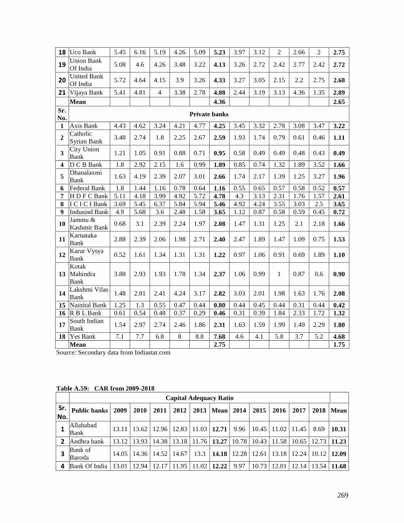
269
18 Uco Bank 5.45 6.16 5.19 4.26 5.09 5.23 3.97 3.12 2 2.66 2 2.75
19 Union Bank
Of India 5.08 4.6 4.26 3.48 3.22 4.13 3.26 2.72 2.42 2.77 2.42 2.72
20 United Bank
Of India 5.72 4.64 4.15 3.9 3.26 4.33 3.27 3.05 2.15 2.2 2.75 2.68
21 Vijaya Bank 5.41 4.81 4 3.38 2.78 4.08 2.44 3.19 3.13 4.36 1.35 2.89
Mean 4.36 2.65
Sr.
No. Private banks
1 Axis Bank 4.43 4.62 3.24 4.21 4.77 4.25 3.45 3.32 2.78 3.08 3.47 3.22
2 Catholic
Syrian Bank 3.48 2.74 1.8 2.25 2.67 2.59 1.93 1.74 0.79 0.61 0.46 1.11
3 City Union
Bank 1.21 1.05 0.91 0.88 0.71 0.95 0.58 0.49 0.49 0.48 0.43 0.49
4 D C B Bank 1.8 2.92 2.15 1.6 0.99 1.89 0.85 0.74 1.32 1.89 3.52 1.66
5 Dhanalaxmi
Bank 1.63 4.19 2.39 2.07 3.01 2.66 1.74 2.17 1.39 1.25 3.27 1.96
6 Federal Bank 1.8 1.44 1.16 0.78 0.64 1.16 0.55 0.65 0.57 0.58 0.52 0.57
7 H D F C Bank 5.11 4.18 3.99 4.92 5.72 4.78 4.3 3.13 2.31 1.76 1.57 2.61
8 I C I C I Bank 3.69 5.45 6.37 5.84 5.94 5.46 4.92 4.24 3.55 3.03 2.5 3.65
9 Indusind Bank 4.9 5.68 3.6 2.48 1.58 3.65 1.12 0.87 0.58 0.59 0.45 0.72
10 Jammu &
Kashmir Bank 0.68 3.1 2.39 2.24 1.97 2.08 1.47 1.31 1.25 2.1 2.18 1.66
11 Karnataka
Bank 2.88 2.39 2.06 1.98 2.71 2.40 2.47 1.89 1.47 1.09 0.75 1.53
12 Karur Vysya
Bank 0.52 1.61 1.34 1.31 1.31 1.22 0.97 1.06 0.91 0.69 1.89 1.10
13
Kotak
Mahindra
Bank
3.88 2.93 1.93 1.78 1.34 2.37 1.06 0.99 1 0.87 0.6 0.90
14 Lakshmi Vilas
Bank 1.48 2.81 2.41 4.24 3.17 2.82 3.03 2.01 1.98 1.63 1.76 2.08
15 Nainital Bank 1.25 1.3 0.55 0.47 0.44 0.80 0.44 0.45 0.44 0.31 0.44 0.42
16 R B L Bank 0.61 0.54 0.48 0.37 0.29 0.46 0.31 0.39 1.84 2.33 1.72 1.32
17 South Indian
Bank 1.54 2.97 2.74 2.46 1.86 2.31 1.63 1.59 1.99 1.49 2.29 1.80
18 Yes Bank 7.1 7.7 6.8 8 8.8 7.68 4.6 4.1 5.8 3.7 5.2 4.68
Mean 2.75 1.75
Source: Secondary data from Indiastat.com
Table A.59: CAR from 2009-2018
Capital Adequacy Ratio
Sr. No.
Public banks 2009 2010 2011 2012 2013 Mean 2014 2015 2016 2017 2018 Mean
1 Allahabad
Bank 13.11 13.62 12.96 12.83 11.03 12.71 9.96 10.45 11.02 11.45 8.69 10.31
2 Andhra bank 13.12 13.93 14.38 13.18 11.76 13.27 10.78 10.43 11.58 10.65 12.73 11.23
3 Bank of
Baroda 14.05 14.36 14.52 14.67 13.3 14.18 12.28 12.61 13.18 12.24 10.12 12.09
4 Bank Of India 13.01 12.94 12.17 11.95 11.02 12.22 9.97 10.73 12.01 12.14 13.54 11.68

270
5 Bank Of
Maharashtra 12.05 12.88 13.35 12.43 12.59 12.66 10.79 11.94 11.2 11.18 13.27 11.68
6 Canara Bank 14.91 13.43 15.38 13.76 12.4 13.98 10.63 10.56 11.08 12.86 13.31 11.69
7 Central Bank
Of India 13.12 12.23 11.64 12.4 11.49 12.18 9.87 10.9 10.4 10.94 9.04 10.23
8 Corporation
Bank 13.61 15.37 14.11 13 12.33 13.68 11.65 11.09 10.56 11.32 11.12 11.15
9 Dena Bank 12.07 12.77 13.41 11.51 11.3 12.21 11.14 10.93 11 11.39 11.48 11.19
10 I D B I Bank 11.57 11.31 13.64 14.58 13.13 12.85 11.68 11.76 11.67 10.7 10.4 11.24
11 Indian Bank 13.98 12.71 13.56 13.47 13.08 13.36 12.64 12.86 13.2 13.64 9.25 12.32
12 Indian
Overseas Bank 13.2 14.78 14.55 13.32 11.85 13.54 10.78 10.11 9.67 10.49 9.25 10.06
13 Oriental Bank
Of Commerce 12.98 12.54 14.23 12.69 12.04 12.90 11.01 11.41 11.76 11.64 10.5 11.26
14 Punjab & Sind
Bank 14.35 13.1 12.94 13.26 12.91 13.31 11.04 11.24 10.91 11.05 10.66 10.98
15 Punjab
National Bank 14.03 14.16 12.43 12.63 12.72 13.19 11.52 12.21 11.28 11.66 9.12 11.16
16 State Bank Of
India 14.25 13.39 11.98 13.86 12.92 13.28 12.44 11.56 13.12 13.11 12.6 12.57
17 Syndicate
Bank 12.68 12.7 13.04 12.24 12.59 12.65 11.41 10.54 11.16 12.03 12.24 11.48
18 Uco Bank 11.93 13.21 13.71 12.35 14.15 13.07 12.68 12.17 9.63 10.93 10.94 11.27
19 Union Bank
Of India 13.27 12.51 12.95 11.85 11.45 12.41 10.8 10.22 10.56 11.79 11.56 10.99
20 United Bank
Of India 13.28 12.8 13.05 12.69 11.66 12.70 9.81 10.57 10.08 11.14 12.62 10.84
21 Vijaya Bank 13.15 12.5 13.88 13.06 11.32 12.78 10.56 11.43 12.58 13.86 13.06 12.30
13.1 11.31
Sr.
No. Private banks
1 Axis Bank 13.69 15.8 12.65 13.66 17 14.56 16.07 15.39 15.29 14.95 16.58 15.66
2 Catholic
Syrian Bank 12.29 10.81 11.22 11.08 12.29 11.54 11 11 10.55 12.15 9.91 10.92
3 City Union
Bank 12.69 13.46 12.75 12.57 13.98 13.09 15.01 16.52 15.58 15.83 16.22 15.83
4 D C B Bank 13.3 14.85 13.25 15.41 13.61 14.08 13.71 14.95 14.11 13.76 15.45 14.40
5 Dhanalaxmi
Bank 15.38 12.99 11.8 9.49 11.06 12.14 8.67 9.59 7.51 10.26 13.87 9.98
6 Federal Bank 20.22 8.36 16.79 16.64 14.73 15.35 15.28 15.46 13.93 12.39 14.87 14.39
7 H D F C Bank 15.69 17.44 16.22 16.52 16.8 16.53 16.07 16.79 15.53 14.55 14.82 15.55
8 I C I C I Bank 15.53 19.41 19.54 18.52 19.72 18.54 17.7 17.02 16.64 17.39 18.42 17.43
9 Indusind Bank 12.55 15.33 15.89 13.85 14.38 14.40 13.83 12.09 15.5 15.31 15.03 14.35
10 Jammu &
Kashmir Bank 14.48 15.89 13.72 13.36 12.83 14.06 12.69 12.57 11.85 10.8 11.42 11.87
11 Karnataka
Bank 13.48 12.37 13.33 12.84 13.22 13.05 13.2 12.41 12.03 13.3 12.04 12.60
12 Karur Vysya
Bank 14.92 14.49 14.41 14.41 14.41 14.53 12.59 14.62 12.17 12.54 14.43 13.27
13
Kotak
Mahindra
Bank
20.01 18.35 19.92 17.52 16.05 18.37 18.83 17.81 16.28 16.77 18.2 17.58
14 Lakshmi Vilas 10.29 14.9 13.19 13.1 12.32 12.76 10.9 11.34 10.67 10.38 9.81 10.62

271
Bank
15 Nainital Bank 13.1 15.68 16.35 15.09 14.43 14.93 15.13 14.86 15.69 12.78 14.95 14.68
16 R B L Bank 42.3 34.07 56.41 23.2 17.11 34.62 14.64 13.52 12.94 13.72 15.33 14.03
17 South Indian
Bank 14.86 15.39 14.01 14 13.91 14.43 12.42 11.92 11.82 12.37 12.7 12.25
18 Yes Bank 16.6 20.6 16.5 17.9 18.3 17.98 14.4 19.7 16.5 17 18.4 17.20
15.83 14.03
Source: : Secondary data from Indiastat.com
A.60: Result of Leverage Ratio from 2009-2018
Minimum Common Equity Leverage ratio
Sr. No.
Public banks 2014 2015 2016 2017 2018 2016 2017 2018
1 Allahabad Bank 7.35 7.57 8.3 8.2 5.57 5.35 5.22 3.65
2 Andhra bank 7.96 7.55 7.83 7.69 5.61 5.52 5.9 4.45
3 Bank of Baroda 8.95 9.8 10.78 9.64 10.08 4.8 4.78 5
4 Bank Of India 6.99 7.59 8.31 7.71 8.52 5.83 5.65 5.8
5 Bank Of Maharashtra 6.69 7.48 7.88 7.28 8.97 5.01 5.01 4.15
6 Canara Bank 7.41 7.37 8.16 9.03 9.63 4.9 5.24 5.52
7 Central Bank Of India 6.47 7.86 8.03 8.62 7.01 5.17 5.07 3.66
8 Corporation Bank 7.66 7.37 7.3 7.99 8.1 --- --- ---
9 Dena Bank 7.43 7.29 7.35 7.43 7.11 --- --- ---
10 I D B I Bank Ltd. 7.78 7.29 7.98 5.63 7.42 --- --- ---
11 Indian Bank 8.25 7.35 7.5 8.3 8.43 --- --- ---
12 Indian Overseas Bank 7.18 6.55 7.1 7.58 6.39 5.12 5.02 3.86
13 Oriental Bank Of
Commerce 8.3 8.09 8.52 7.59 7.46 --- ---- ----
14 Punjab & Sind Bank 7.27 8.48 8.48 9.14 7.65 4.7 5.4 4.93
15 Punjab National Bank 9 9.14 8.48 8.17 5.95 5.88 5.09 3.85
16 State Bank Of India 7.4 8.75 9.81 9.82 9.68 5.24 5.37 5.38
17 Syndicate Bank 8.29 7.53 7.01 7.5 7.56 4.08 5.17 5.04
18 Uco Bank 8.5 8.94 7.52 7.64 8.23 3.9 4.11 4.18
19 Union Bank Of India 7.28 7.25 7.96 7.76 7.64 5 5.4 4.96
20 United Bank Of India 6.54 7.52 7.74 8.46 8.39 4.31 4.34 4.26
21 Vijaya Bank 8.12 7.6 8.31 8.44 10.36 5.3 5.36 6.26
Sr.
No. Private banks
1 Axis Bank ---- ----- ----- ---- 11.8 8.33 8.22 8.64
2 Catholic Syrian Bank ---- ----- ---- ----- 9.45 ---- ---- 4.32
3 City Union Bank ---- ----- ----- ---- 13.92 9.09 9.42 9.82
4 D C B Bank ---- ----- ---- ----- ---- --- ---- 7.22
5 Dhanalaxmi Bank ---- ----- ----- ---- ---- 3.13 4.26 4.92
6 Federal Bank ---- ----- ---- ----- 8.85 7.68 6.91 7.97
7 H D F C Bank ---- ----- ----- ---- 12.25 8.87 8.77 9.19
8 I C I C I Bank ---- ----- ---- ----- 14.43 9.06 9.79 9.83

272
9 Indusind Bank ---- ----- ----- ---- 13.42 9.33 9.26 9.02
10 Jammu & Kashmir Bank ---- ----- ---- ----- ----- ---- ---- 6.12
11 Karnataka Bank ---- ----- ----- ---- ---- 6 6.83 6.65
12 Karur Vysya Bank ---- ----- ---- ----- 11.85 6.54 7.15 8.49
13 Kotak Mahindra Bank ---- ----- ----- ---- 17.5 12.1 12.6 13.27
14 Lakshmi Vilas Bank ---- ----- ---- ----- 8.05 ---- ---- 9.81
15 Nainital Bank ---- ----- ----- ---- ----- 8.21 7.25 7.24
16 R B L Bank ---- ----- ---- ----- ----- 6.58 7.31 8.87
17 South Indian Bank ---- ----- ----- ---- ------ 5.55 5.99 5.78
Yes Bank ---- ----- ---- ----- 9.7 6.6 8.84 8.54
Source: Secondary data from Indiastat.com
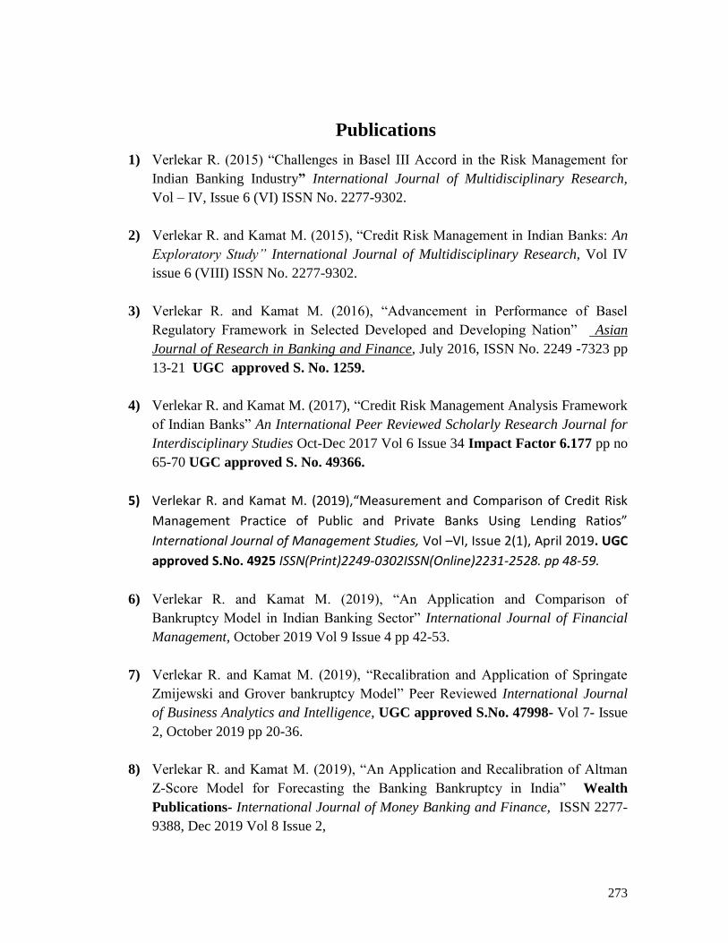
273
Publications
1) Verlekar R. (2015) “Challenges in Basel III Accord in the Risk Management for
Indian Banking Industry” International Journal of Multidisciplinary Research,
Vol – IV, Issue 6 (VI) ISSN No. 2277-9302.
2) Verlekar R. and Kamat M. (2015), “Credit Risk Management in Indian Banks: An
Exploratory Study” International Journal of Multidisciplinary Research, Vol IV
issue 6 (VIII) ISSN No. 2277-9302.
3) Verlekar R. and Kamat M. (2016), “Advancement in Performance of Basel
Regulatory Framework in Selected Developed and Developing Nation” Asian
Journal of Research in Banking and Finance, July 2016, ISSN No. 2249 -7323 pp
13-21 UGC approved S. No. 1259.
4) Verlekar R. and Kamat M. (2017), “Credit Risk Management Analysis Framework
of Indian Banks” An International Peer Reviewed Scholarly Research Journal for
Interdisciplinary Studies Oct-Dec 2017 Vol 6 Issue 34 Impact Factor 6.177 pp no
65-70 UGC approved S. No. 49366.
5) Verlekar R. and Kamat M. (2019),“Measurement and Comparison of Credit Risk
Management Practice of Public and Private Banks Using Lending Ratios”
International Journal of Management Studies, Vol –VI, Issue 2(1), April 2019. UGC
approved S.No. 4925 ISSN(Print)2249-0302ISSN(Online)2231-2528. pp 48-59.
6) Verlekar R. and Kamat M. (2019), “An Application and Comparison of
Bankruptcy Model in Indian Banking Sector” International Journal of Financial
Management, October 2019 Vol 9 Issue 4 pp 42-53.
7) Verlekar R. and Kamat M. (2019), “Recalibration and Application of Springate
Zmijewski and Grover bankruptcy Model” Peer Reviewed International Journal
of Business Analytics and Intelligence, UGC approved S.No. 47998- Vol 7- Issue
2, October 2019 pp 20-36.
8) Verlekar R. and Kamat M. (2019), “An Application and Recalibration of Altman
Z-Score Model for Forecasting the Banking Bankruptcy in India” Wealth
Publications- International Journal of Money Banking and Finance, ISSN 2277-
9388, Dec 2019 Vol 8 Issue 2,
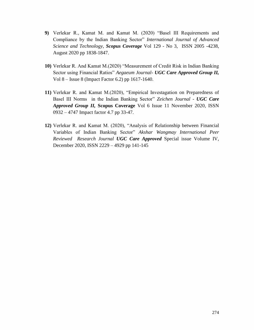
274
9) Verlekar R., Kamat M. and Kamat M. (2020) “Basel III Requirements and
Compliance by the Indian Banking Sector” International Journal of Advanced
Science and Technology, Scopus Coverage Vol 129 - No 3, ISSN 2005 -4238,
August 2020 pp 1838-1847.
10) Verlekar R. And Kamat M.(2020) “Measurement of Credit Risk in Indian Banking
Sector using Financial Ratios” Aegaeum Journal- UGC Care Approved Group II,
Vol 8 – Issue 8 (Impact Factor 6.2) pp 1617-1640.
11) Verlekar R. and Kamat M.(2020), “Empirical Investagation on Preparedness of
Basel III Norms in the Indian Banking Sector” Zeichen Journal - UGC Care
Approved Group II, Scopus Coverage Vol 6 Issue 11 November 2020, ISSN
0932 – 4747 Impact factor 4.7 pp 33-47.
12) Verlekar R. and Kamat M. (2020), “Analysis of Relationship between Financial
Variables of Indian Banking Sector” Akshar Wangmay International Peer
Reviewed Research Journal UGC Care Approved Special issue Volume IV,
December 2020, ISSN 2229 – 4929 pp 141-145
Copyright © 2022 FDOKUMEN