A stratified model for the assessment

of meteorologically adjusted trends

of surface ozone

DAN IELA COCCH I ,* , � ENR ICO FABR IZ I �� and

CARLO TR IV I SANO �

�Dipartimento di Scienze Statistiche ‘‘Paolo Fortunati’’, Universita di Bologna, Via delle BelleArti, 41, I-40127 Bologna, Italy

E-mail: cocchi@stat.unibo.it��Dipartimento di matematica, statistica, informatica e applicazioni, Universita di bergamo

Received October 2003; Revised December 2004

We consider the problem of assessing long-term trends of ozone concentrations measured on a

single site located in an urban area. Among the many methods proposed in the literature toeliminate the confounding effect of changing weather conditions, we employ a stratification ofdaily maxima based on regression trees. Within each stratum conditional independence and

Weilbull distribution are assumed for maxima. Long-term trend is defined non-parametricallyby the sequence of yearly medians. Models are estimated following the Bayesian approach.The alternative assumptions of common and stratum specific trends are compared and amodel with common trend for all strata is selected for the analyzed real dataset. The condi-

tional independence assumption is checked by the comparison with a model including anautoregressive component.

Keywords: McMC, regression trees, Weibull distribution

1352-8505 � 2005 Springer Science+Business Media, Inc.

1. Introduction

In this paper we face the problem of determining the trend of daily maxima of ozoneconcentrations measured in an urban area. Because of the close dependence betweenozone and weather conditions, a major issue is to assess whether any observed trendin the data is due to variation in the emissions or to particular climatic conditions.

This subject has been widely discussed in literature and comprehensive reviews areavailable (Thompson et al., 2001; Cocchi and Trivisano, 2002). The influence ofclimatic conditions on ozone concentrations has been eliminated by using a variety

*Corresponding author.

Environmental and Ecological Statistics 12, 195–208, 2005

1352-8505 � 2005 Springer Science+Business Media, Inc.

of techniques: supervised and unsupervised classification (usually referred to asstratified approach), linear and non-linear regression, extreme value modeling.

Huang and Smith (1999) propose a supervised stratified method based on regressiontrees consisting in two steps: first, a regression tree is introduced to partition the dailymaxima into groups with an homogeneous ozone level and the same meteorologicalconditions, subsequently the trend is evaluated by means of a set of alternative linearhomoschedastic random effects models, some of which with a different trend withineach group. This approach has the merit of allowing for the estimation of differenttrends at different levels of ozone concentration and weather conditions.

We propose a model for trend inspection which follows the basic idea of Huang andSmith (1999). Similarly to these authors we introduce a tree based partitioning ofobservations, but we assume that the daily maxima of ozone concentrations areWeibulldistributed and propose a random effects model for the median of this distribution,where the considered effects are represented by the homogeneous ozone regimesresulting from tree partitioning and the year. In order to model directly the median ofobservations we introduce a suitable re-parameterization of the Weibull distribution.

The trend of ozone maxima is then evaluated as the sequence of yearly variationsof medians within meteorologically homogeneous groups of observations: ourapproach then is free of any hypothesis about the shape of trend.

The Weibull distribution arises naturally in the context of maxima; moreover itrepresents a flexible assumption since, for different values of its parameters, it rangesfrom approximately normal to highly skewed forms. It may then be expected thatour models would fit well on the tails of distributions and provide a more preciseestimation of high percentiles and exceedances.

Our approach is somewhat close to the proposal of Cox and Chu (1993), whoassume a Weibull distribution for daily maxima in which the logarithm of thequasi-scale parameter is modeled as a linear function of time (among meteorologicalcovariates). We note that, even though based on the same distributional assumption,their approach is not stratified and employs a different definition of trend.

As regards inference, we adopt a Bayesian approach. Posterior summaries areobtained by means of Gibbs sampling routines, as they are implemented in thesoftware BUGS (Spiegelhalter et al., 1996).

We apply our method of trend assessment to the series of daily maxima of hourlyozone concentrations measured from a single monitoring site located in the city ofBologna, Italy, in the period 1994–2002.

The paper is organized as follows. Section 2 contains a description of the data,while in Section 3 the proposed models are introduced. In Section 4 results abouttrend estimation are discussed along with model checks and measures of its adequacyin the tails of the distributions. Particular attention is devoted to the analysis of thesensitivity of results to the assumption of conditional independence of observationswithin ozone-homogeneous groups.

2. The data

In this paper we analyze the series of daily maxima of ozone concentrations over themetropolitan area of Bologna, in the North of Italy, in the period 1994–2002.

Cocchi, Fabrizi, Trivisano196

Data have been gathered, and their quality assessed, by the ARPA (RegionalEnvironment Protection Agency) of the Emilia Romagna region, that is charged bythe Italian law with all monitoring and protection policies related to air pollution.

Maxima are calculated on the basis of hourly measurements from a single mon-itoring site situated in Giardini Margherita, a park near to the centre of the city. Weconsider exclusively data gathered during the ozone seasons (from April 1st toOctober 31st) yielding a gross total of 1926 observations (Fig. 1). For 88 observa-tions the maximum is not calculated because of measurement failures or othercauses. We calculate regression trees simply discarding the missing observations.Then, we impute the 88 missing values using the selected regression tree model.These imputations are needed to make comparison between models based on con-ditional independence assumption (Section 3) and models relaxing this assumption(Section 4.4) possible.

The meteorological variables we make use of are collected at the surface weatherstation of Borgo Panigale, a few kilometers away from the monitoring site ofGiardini Margherita. We consider the following daily summaries: minimum, maxi-mum and average temperature (�C), minimum, maximum and average relativehumidity (%), precipitations (mm), maximum and average wind speed (m/s), pre-valent wind direction (� from N), pressure (mb), minimum, maximum and averagecloud coverage (octaves). Lagged values (1 and 2 days) for all the meteorologicalvariables are considered.

A further variable indicating the day within the year (1 for April 1st, . . . ; 214 forOct 31st) is considered to reflect seasonal effects.

Missing data are present in the series of meteorological variables as well. In thiscase we do not propose any imputation, since they are not needed in building theregression tree.

0

50

100

150

200

250

300

Apr-94 Apr-95 Apr-96 Apr-97 Apr-98 Apr-99 Apr-00 Apr-01 Apr-02

µg/m

3

Figure 1. Ozone daily maxima of hourly concentrations in Bologna, ozone seasons, from1994 to 2002.

Models for assessing meteorologically adjusted trends of surface ozone 197

3. Stratified modelling

3.1 Identification of homogeneous regimes

Partitioning methods based on classification and regression trees have gained a widepopularity in environmental statistics, since they are particularly suitable to explorethe non-linear relationship between pollutants concentrations and weather (Burrowset al., 1995); moreover they perform rather well in forecasting occurrences of highconcentrations. However, trees cannot be directly employed in trend assessment,since a trend component cannot be included into this class of models. A remarkableattempt to exploit the power of regression trees in meteorological adjustment for thepurpose of trend investigation is carried out by Huang and Smith (1999). Workingon the well-known Chicago ozone data, they first partition the observations intohomogeneous clusters using a regression tree method (Clark and Pregibon, 1991).

Following Huang and Smith, we build a regression tree for ozone daily maximausing the set of meteorological covariates described in Section 2. We follow theCART approach (Breiman et al., 1984), that does not make use of any distributionalassumption. At each node (parent) of the tree, data are partitioned into twohomogeneous subsets (left child and right child) on the basis of the squared loss (L2),that is by maximising

DL2 ¼ L2parent � L2

leftchild þ L2rightchild:

The usual cost-complexity criterion described in Breiman et al. (1984) is employed forpruning the tree; 10-fold cross-validation is employed to select the degree of pruning.

3.2 Models for the trend

Let us denote the vector of daily maxima with y. For each vector component weassume that

yijki; ni�indWeibull ki; nið Þ i¼ 1;:::;N¼ 1926:

We introduce a parameterization that expresses the density as a function of thedistribution’s median Me yijki; xiið Þ ¼ ki:

f yijki; nið Þ ¼ niknii

ðln 2Þyni�1i exp � yi

ki

� �ni

ln 2ð Þ !

: ð1Þ

Each distribution (1) is characterized by the following moments:

E yijki; nið Þ ¼ k�1i ln 2ð Þ1=niC 1þ 1=nið Þ

V yijki; nið Þ ¼ k�2i ln 2ð Þ2=ni C 1þ 2=nið Þ � C2 1þ 1=nið Þ� �

:

We consider two different models for the logarithm of the median: an interactionmodel with independent group by year random effects (referred to as model 1) and

Cocchi, Fabrizi, Trivisano198

an additive model assuming independent year and group effects (model 2), whichmimic the first two ANOVA models considered by Huang and Smith (1999).

More formally, model 1 is characterized by

ln kð Þ ¼Wu

where k ¼ k1; k2; . . . ; kNð ÞT and u is aH = (G · P) dimensional random vector (G isthe number of groups identified by the tree, while P is the number of years con-sidered by this study). The N · H matrix W is defined, using a block notation, asW ¼ W1j . . . jWPð Þ; the generic element of Wpðp ¼ 1; . . . ; PÞ is a N · G matrix that canbe described as

ðwijð pÞ Þ ¼1 if day i falls in year p and cluster j, j=1,...,G0 otherwise

n:

On its turn, model 2 is characterized by

ln kð Þ ¼ aþ Xbþ Zc ð2Þ

where X is a N · (G ) 1) design matrix whose generic element is defined as

xij� �

¼ 1 if day i falls incluster j+10 otherwise

nð3Þ

and Z a N · (P ) 1) matrix for which we have

zij� �

¼ 1 if day i falls inyear j+10 otherwise

nð4Þ

The general intercept a is introduced to avoid multicollinearity of year and groupeffects.

We define the trend as the sequence of the parameters associated to year effects,thus avoiding the assumption on any functional form. Note that model 1 corre-sponds to the hypothesis of a group specific trend, while model 2 assumes a commontrend for all groups identified by the tree.

We also consider a third benchmark model (model 3), formalizing the hypothesisof absence of trend, which mimics model 5 in Huang and Smith (1999); it is char-acterized by

ln kð Þ ¼ aþ Xb

As regards the shape parameters, we assume that they are group specific but constantover the years within a given group, as follows

n ¼ X�f ð5Þ

where f ¼ f1; . . . ; fGð ÞT , while X* is a N · Gmatrix whose generic element is given by

x�ij

� �¼ 1 if day i falls in cluster j

0 otherwise

n

Assumption (5) reflects the idea of differently shaped distributions at different levelsof the process but with the same shape along time. Since the coefficient of variationof the Weibull distribution depends only on the shape parameter, (5) implies that thecoefficient of variation is group-specific, that is, it varies with the level of the process.

Models for assessing meteorologically adjusted trends of surface ozone 199

Assumption (5) is more flexible than that taken by Cox and Chu (1993), whohypothesize a common shape parameter (and therefore coefficient of variation) forthe whole sample.

For the specification of prior distributions, we assume, for all models, the fol-lowing prior for the shape parameters:

fj �ind

Gamma 3; 1ð Þ j ¼ 1; . . . ;G ð6Þ

implying E fj

� �¼ 3; V fj

� �¼ 3. This distribution is centered on the value of fj for

which the shape of the Weibull distribution is similar to that of the Normal (sym-metric tails), but is sufficiently diffuse to give support also to the assumption ofskewed distributions.

Parameters associated to random effects are given in all cases a Normal priordistribution centered on 0, while assumptions on their precisions change from modelto model. In particular in model 1 we specify that

ujs �indN 0;Cð Þ ð7Þ

where the precision matrix C is block diagonal and can be written as

C ¼ blockdiag s1IG; . . . ; sPIGð Þ:

For the precision parameters s ¼ s1; s2; . . . ; sPð ÞT we assume that it has a prioriindependent components distributed as

si �indGamma 0:1; 0:1ð Þ ð8Þ

that is, we assume a common prior distribution for the group intercept within thesame year while a diffuse Gamma is chosen for the precisions in s; we remark thatthis non-informative ‘‘reference’’ solution is designed mostly for computationalconvenience.

In model 2 we introduce the following priors:

a � N 0; 0:01ð Þb m1 � N 0; m1Ið Þjm1 � Gamma 0:1; 0:1ð Þc m2 � N 0; m2Ið Þjm2 � Gamma 0:1; 0:1ð Þ ð9Þ

thus assuming common distributions for year and group effects. Consistently, thesame prior assumptions on a and b are introduced in model 3.

We calculate all posterior distributions by using Markov chain Monte Carlo(McMC) sampling algorithms, as implemented in the software BUGS (Spiegelhalteret al., 1996), based on Gibbs sampling. The selected prior distributions have stan-dard functional forms and this lead to log-concave full conditionals in all cases. Weexamine the sensitivity of posteriors to changes in (6)–(9) without finding anythingsubstantial. So, such priors can be considered as non-informative. As regards theassessment of convergence we consider the multiple chain approach suggested byGelman and Rubin (1992), running three different chains with well separated starting

Cocchi, Fabrizi, Trivisano200

points for each model. The visual inspection of chains paths and the modifiedGelman and Rubin statistic (Brooks and Gelman, 1998) are the convergenceassessment tools adopted. We run 10,000 iterations for each chain, discarding onaverage a conservative ‘‘burn in’’ of 3000, thus yielding approximately 20,000 drawsfrom the posterior of each model.

4. Model choice and discussion of empirical results

4.1 The regression tree

On the basis of the CART method described in Section 3.1 we build the tree shownin Fig. 2.

As should be expected according to the photochemical nature of reactions leadingto concentration of surface ozone, maximum temperature and other related variablesare responsible for the most important splits in the tree, but also cloud coverage andhumidity play a relevant role in determining homogeneous ozone regimes.

Our optimal tree identifies 11 groups with very different sizes, ranging from 45 upto 443. The classification of daily maxima by group and year is reported in Table 1.

The hierarchical structure of prior distributions of the models described in Section3.2 is very helpful for the estimation of parameters as it allows, at the price of someshrinkage, for borrowing information across groups.

4.2 Model comparisons

Within the Bayesian framework, models are usually compared by means of the BayesFactors (BF). Since they are rather difficult to compute, a large sample approxi-mation of 2logBF is given by the Bayes Information Criterion (DBIC) defined asfollows:

DBICModeli;Model3 ¼ 2 logsupModeli f yjhið ÞsupModel3 f yjh3ð Þ

� pi � p3ð Þ log n i ¼ 1; 2 ð10Þ

(see Schwartz, 1978). We compare our models by means of (10) that, moreover, hasthe merit of making no reference to prior assumptions. We note that in (10) hi(i=1,2,3) is the multi-dimensional parameter indexing the likelihood associated toeach model and pi is the number of parameters of the distribution at the lowest levelof the hierarchy. The null model against which the others are compared is, in ourcase, model 3. Model comparisons are summarized in Table 2.

The Bayes Information Criterion (10) indicates that model 2 is the best, sup-porting the hypothesis of a significant variation of ozone levels over the years, evenwithin the homogeneous groups identified by the tree. It is also apparent that model2 is to be preferred to model 3. This evidence tells us that trends in groups are not ‘‘sodifferent’’ to justify the introduction of group-specific trends.

This is rather clear by looking at Fig. 3 where posterior means of medianparameters obtained under model 1 and model 2 are compared by group and year.

Models for assessing meteorologically adjusted trends of surface ozone 201

Figure

2.Regressiontree

fortheBolognaozonemaxim

a.

Cocchi, Fabrizi, Trivisano202

4.3 Model adequacy checks

The adequacy of the selected model is checked following a posterior predictiveapproach based on Bayesian p-values (Rubin, 1984) that can be easily implementedon the basis of the McMC output.

Our primary goal is ozone trends evaluation on the basis of yearly variations ofmedians within meteorologically homogeneous groups of observations. For thisreason, we first check the ability of the model to predict the observed medians. Sinceour models are parameterized in terms of medians, this check is essentially about theadequacy of the amount of shrinkage introduced.

We define the discrepancy measure:

D y; kð Þ ¼XNi¼1

d yi � kið Þ

where d(.) is the indicator function. The p-value associated to D for model 2 is 0.62, avalue that can be regarded as acceptable.

Table 1. Daily maxima classified by group and year.

Year

Group 1994 1995 1996 1997 1998 1999 2000 2001 2002

1 39 63 60 50 53 44 39 66 50 4642 6 7 5 14 3 1 4 7 3 50

3 23 24 29 18 30 18 14 19 28 2034 25 26 15 7 9 17 21 10 26 1565 8 19 16 4 9 16 16 11 13 1126 37 20 23 28 22 22 34 18 25 229

7 15 12 19 20 11 23 16 19 20 1558 12 15 16 22 18 26 27 15 20 1719 17 34 21 46 30 29 24 38 18 257

10 3 8 6 1 15 8 13 6 6 6611 3 12 4 4 14 10 6 5 5 63

214 214 214 214 214 214 214 214 214 1926

Table 2. Model comparisons by means of DBIC.

DBIC

Model 1 vs. Model 3 )235.6Model 2 vs. Model 3 241.9

Models for assessing meteorologically adjusted trends of surface ozone 203

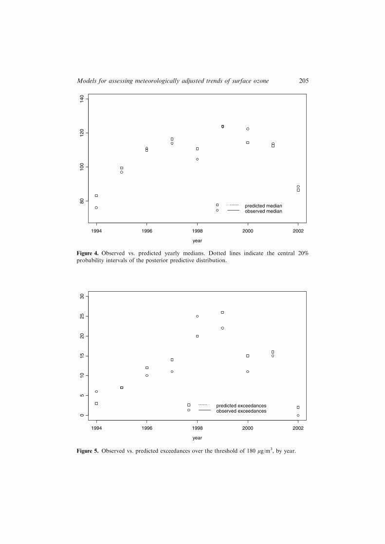
On the basis of the posterior predictive distribution we compute also the yearlymedians of ozone concentrations predicted under model 2. They are plotted againstthe observed ones in Fig. 4.

Dotted lines indicate the 40th and 60th percentiles of the posterior predictivedistributions.

From Fig. 4 we can appreciate how observed yearly medians are well predicted bythe model. Moreover, the shape of the meteorologically adjusted trend of medians,as plotted in Fig. 3, is different from the observed trend of yearly medians. Forinstance, the observed increase in the annual median from 1996 to 1997 can becontrasted with a reduction in the standardized common trend. The increase canthen be ascribed to the peculiar climatic conditions of that year.

This results confirm the commonly recognized need to standardize for the mete-orology before evaluating the long-term trends of ozone concentrations.

On the basis of the posterior predicted distribution, we calculate the annualnumber of exceedances over the threshold of 180 lg/m3 predicted by the model. Thisthreshold is explicitly considered by the Italian law as a ‘‘warning level’’ for theozone concentrations. The number of predicted vs. actual exceedances is plotted inFig. 5. The fitting is good, showing that the selected model behaves well also in theright tail of the distribution.

year1994 1996 1998 2000 2002

8590

9510

011

0

Group 1

year1994 1996 1998 2000 2002

7080

9010

011

012

0

Group 2

year1994 1996 1998 2000 2002

6065

7075

8085

Group 3

year1994 1996 1998 2000 2002

3540

4550

55

Group 4

year1994 1996 1998 2000 2002

6070

80

Group 5

year1994 1996 1998 2000 2002

100

110

120

130

140

Group 6

year1994 1996 1998 2000 2002

9010

011

012

0

Group 7

year1994 1996 1998 2000 2002

100

120

140

160

Group 8

year1994 1996 1998 2000 2002

120

130

140

150

160

170

Group 9

year1994 1996 1998 2000 2002

150

170

190

210

Group 10

year1994 1996 1998 2000 2002

130

140

150

160

170

180

Group 11

MODEL 1MODEL 2

Figure 3. Posterior means of medians under model 1 and model 2, by group and year.

Cocchi, Fabrizi, Trivisano204

year

1994 1996 1998 2000 2002

05

1015

2025

30

predicted exceedancesobserved exceedances

Figure 5. Observed vs. predicted exceedances over the threshold of 180 lg/m3, by year.

year

1994 1996 1998 2000 2002

8010

012

014

0

predicted medianobserved median

Figure 4. Observed vs. predicted yearly medians. Dotted lines indicate the central 20%probability intervals of the posterior predictive distribution.

Models for assessing meteorologically adjusted trends of surface ozone 205

4.4 Sensitivity to the conditional independence assumption

In Section 3, we grounded the assessment of trends on the assumption that dailymaxima are independent given the ‘‘group by year’’ specific medians (and the shapeparameters). This assumption may represent an oversimplification and be, to someextent, inadequate due to the strong serial autocorrelation shown by the time seriesof daily maxima. In this section, we investigate whether the possible failure of theassumption of conditional independence affects the assessment of long-term trends.

To do this, we generalize the selected model 2 by introducing an AR(1) componentin (2). That is, we replace (2) by

lnðkÞ ¼ aþ Xbþ ZcþUe

where X and Z are defined according to (3) and (4); the N · N design matrix U is ablock diagonal one defined as U ¼ blockdiag U1; . . . ;Up

� �where each Up is a Np · Np

(Np being the number of maxima in year p) matrix whose generic element can bedescribed as

uij pð Þ� �

¼ 0 if j > iq i�jj j otherwise

�:

We leave the prior assumptions of (9) unchanged and specify the followingdistribution for e:

ejx � N 0;xINð Þ:

As regards hyper-parameters we assume that

x � Gamma 0:1; 0:1ð Þq � Uniform �1; 1ð Þ:

We refer to this model as model 4.The posterior means and standard deviations (SD) of parameters of model 2 and 4

are listed in Table 3, from which it is evident that all parameters associated to yeareffects are very close in the two cases.

Table 3. Posterior means and SD of parameters from model 2 and model 4.

Model 2 Model 4

Posterior mean Posterior SD Posterior mean Posterior SD

a 4.433 0.019 4.371 0.028c2 0.134 0.021 0.139 0.037c3 0.254 0.022 0.258 0.036

c4 0.201 0.022 0.223 0.038c5 0.166 0.022 0.187 0.041c6 0.3 0.021 0.304 0.037

c7 0.208 0.021 0.238 0.041c8 0.209 0.021 0.237 0.046c9 0.008 0.023 0.032 0.045

Cocchi, Fabrizi, Trivisano206

5. Conclusions

We discuss a method for long-term ozone trend detection that can be thought as adevelopment of the stratified approach of Huang and Smith (1999) and uses the samedistributional assumption of Cox and Chu (1993), which is still employed as thereference method for trends assessment of ozone concentrations by the US EPA(Thompson et al., 2001). Emphasis is given to testing whether there is evidence infavour of separate trends at different process levels or not.

We apply the method to real data coming from a single monitoring station inBologna, Italy, over the period 1994–2002. The analysis highlights the need of stan-dardizing for the weather when assessing the long-term trend of ozone concentrations.In fact we found that the standardized trend behaves differently from the yearlymedian of observations. For instance, the observed median of daily maxima in 1997 ishigher than that of 1996 (Fig. 4), but this rise is due only to climatic conditions as thestandardizedmedians under the selectedmodel are lower in 1997 than in 1996 (Fig. 3).

We consider models with either common or separate trends for different homo-geneous ozone regimes and select the most suitable one on the basis of the data. Theydid not provide sound evidence in favour of specific trends after cancelling out theeffect of weather. Therefore, at present, a common trend assumption provides thebetter description of long-term time pattern of ozone daily maxima for the datasetconsidered.

In this paper, we study ozone trend assessment using data from the single moni-toring site present in the considered urban area. Often monitoring sites are part of anetwork of stations distributed over larger areas. It would be then interesting toextend the methodology presented here to the assessment of a global trend over thenetwork, using tools such as multivariate regression trees for standardization andmodels in which spatial dependence is taken into consideration.

Acknowledgments

The research leading to this paper has been partially funded by a 2002 grant (Sec-tor 13: Economics and Statistics, Project no. 7, protocol no. 2002134337_01 forResearch Projects of National Interest by MIUR). We thank the ARPA staff andMarco Deserti in particular, for their useful advices and comments on variousparts of this research. Thanks are due to the Editor and to an anonymous refereefor comments and suggestion which helped us in improving the manuscript.

References

Breiman, L., Friedman, J.H., Olshen, R.A., and Stone, C.J. (1984)Classification and Regression

Trees, Wadsworth, California.Burrows, W.R., Benjamin, M., Beauchamp, S., Lord, E.R., McCollor, D., and Thompson, B.

(1995) CART decision tree statistical analysis and prediction of summer season

maximum surface ozone for the Vancouver, Montreal and Atlantic Regions of Canada.Journal of Applied Meteorology, 34, 1848–62.

Models for assessing meteorologically adjusted trends of surface ozone 207

Brooks, S.P. and Gelman, A. (1998) Alternative methods for monitoring convergence of

iterative simulation. Journal of Computational and Graphical Statistics, 7, 434–55.Clark, L.A. and Pregibon, D. (1991) Tree-based models. In Statistical Models in S, J.M.

Chambers and T.J. Hastie (eds.), Wadsworth, California, pp. 377–420.

Cocchi, D. and Trivisano, C. (2002) Ozone. In Encyclopedia of Environmetrics, A.H. El-Shaarawi and W.W. Piegorsch (eds.), Wiley, Chicester.

Cox, W.M. and Chu, S.H. (1993) Meteorologically adjusted trends in urban areas: a

probabilistic approach. Atmospheric Environment, 27B, 425–34.Gelman, A. and Rubin, D.B. (1992) Inference from iterative simulation using multiple

sequence. Statistical Science, 7, 457–72.Huang, L.S. and Smith, R.L. (1999) Meteorologically-dependent trends in urban ozone.

Environmetrics, 10, 103–18.Rubin, D.B. (1984) Bayesianly justifiable and relevant frequency calculations for the empirical

statistician. Annals of Statistics, 12, 1151–72.

Schwartz, G. (1978) Estimating the dimension of a model. Annals of Statistics, 6, 461–64.Spiegelhalter, D.J., Thomas, A., Best, N., and Gilks, W.R. (1996) BUGS: Bayesian Inference

Using Gibbs Sampling, version 0.50. Technical Report, Medical Research Council

Biostatistic Unit, Institute of Public Health, Cambridge University.Thompson, M.L., Reynolds, J., Cox, L.H., Guttorp, P., and Sampson, P.D. (2001) A review

of statistical methods for the meteorological adjustment of tropospheric ozone.

Atmospheric Environment, 37, 617–30.

Biographical sketches

Dr. Daniela Cocchi is Professor of Statistics in the Faculty of Statistics at theUniversity of Bologna. She received her degree in statistics in 1975 from theUniversity of Bologna and her Ph.D. in Statistics from the Universite Catholique deLouvain in 1999. Her research interests are in finite population inference, Bayesianstatistics and environmental statistics.

Dr. Enrico Fabrizi is Assistant Professor in the Faculty of Economics of theUniversity of Bergame. He received his degree in statistics in 1996 from the Uni-versity of Bologna and his Ph.D. in Statistics from the University of Bologna in2001. His research interests are in finite population inference, Bayesian statistics andsmall area estimation.

Dr. Carlo Trivisano is Assistant Professor in the Faculty of Statistics at theUniversity of Bologna. He received his degree in statistics in 1991 from theUniversity of Bologna and his Ph.D. in Statistics from the University of Bologna in1997. His research interests are in recursive partitioning methods, Bayesian statisticsand environmental statistics.

Cocchi, Fabrizi, Trivisano208