The Quest for Quality: A Quality Adjusted Dynamic Regulatory Mechanism

The Quest for Quality: A Quality AdjustedDynamic Regulatory Mechanism

GIANNI DE FRAJA

Department of EconomicsUniversity of Leicester

Leicester LE1 7RH, United [email protected]

Dip. SEFEMEQUniversita di Roma “Tor Vergata”

I-00133 Roma, Italy

ALBERTO IOZZI

Dip. SEFEMEQUniversita di Roma “Tor Vergata”

I-00133 Rome, [email protected]

In situations where quality is fixed, the widely used RPI-X regulatory mech-anism has a number of desirable properties, such as convergence to a secondbest optimum. Theoretical analysis of this mechanism in the case of endogenousquality is limited and therefore regulators have typically imposed constraintson the firm’s quality choice in ad hoc manners, either by mandating qualitylevels, or by including quality adjustment factors in the RPI-X mechanism. Inthis paper, we construct the rigorous theoretical counterpart of these mannersof including quality measures in the constraints faced by a regulated firm. Thismechanism converges to second best optimum. It works by offering the firmtrade-offs between prices and qualities based on the choice it made in the previousperiod; however, reflecting the practical problem valuing quality, the infor-mational requirement to select these trade-offs appropriately is qualitativelystronger than in the fixed quality case. Moreover, even when the informationalproblem can be overcome, we identify a further potential pitfall in the approachtaken in practice by regulators, and show that, in order to avoid it, theregulated firm should be subject to an additional constraint, which we labelthe distance constraint, and which can be interpreted as requiring the firms tochoose prices and qualities within a band in every period.

An earlier version of the paper was presented in Padua, Turin and Brescia, and at the2005 EARIE Conference (Porto). As well as audiences there, we thank Ali al-Nowaihi,Paolo Bertoletti, and especially two referees and one coeditor of this Journal for helpfulcomments.

C© 2008, The Author(s)Journal Compilation C© 2008 Wiley Periodicals, Inc.Journal of Economics & Management Strategy, Volume 17, Number 4, Winter 2008, 1011–1040

1012 Journal of Economics & Management Strategy

1. Introduction

The quality of firms’ output has received a great deal of attention, both inthe economics literature, where the analysis of quality choices by firmshas been a cornerstone of the modern theory of industrial organisationsince its early days,1 and in the practice of regulation: in many countries,utility regulators spend a great deal of effort trying to influence thequality supplied by the regulated firms under their jurisdiction.

However, relative to the large theoretical literature examiningregulated firms (Armstrong and Sappington, 2005), rigorous theoreticalanalyses of applied mechanisms for quality choices in regulated firmshave been scarcer (for a recent survey, see Sappington, 2005), offeringregulators limited sound theoretical guidance in this area. Regulatorshave therefore resorted to taking an ad hoc approach towards qualityregulation, either imposing quality standards, or explicitly or implic-itly linking the allowed price level to quality improvements (see, forinstance, Ofwat, 2002; more examples are discussed in Section 3). Thisad hoc approach constitutes a sharp contrast with the relative sophis-tication of RPI-X price cap regulation which has become increasinglypopular since its first use in the United Kingdom at the beginningof the 1980s. As noted by Bradley and Price (1989), the RPI-X pricecap is the practical counterpart of Vogelsang and Finsinger’s seminaltheoretical contribution (1979, VF in what follows). VF study a dynamicmodel of price regulation (with fixed qualities), and show that anappropriately designed price cap mechanism aligns the firm’s trade-offsto the regulator’s, and induces the firm to choose, as time goes by, pricescloser and closer to those which an omniscient regulator concernedsolely with consumers’ welfare would choose.

VFs analysis and RPI-X price cap regulation are founded on theprinciple that the firm is the decision maker best placed to evaluatethe trade-offs between costs and social value for its different products,and therefore to take decision regarding relative prices. Clearly, thisis just as true for quality. Our paper therefore extends formally VFsanalysis to lay a theoretical foundation of the regulation of quality onthe same principle that the firm has superior knowledge of its costand demand functions, with the aim of obtaining a mechanism thatis both theoretically rigorous and readily applicable in practice. Whilesharing its properties of being based on the previous period consumers’valuation and not requiring knowledge of the cost function, a qualityadjusted price-cap mechanism has a fundamental limitation relativeto the VF mechanism. The constraint it imposes on the firm creates

1. Early contributions are Spence (1975) and Mussa and Rosen (1978) for the monop-olist, and Shaked and Sutton (1982) and Gabszewicz and Thisse (1979) for the oligopolycase.

The Quest for Quality 1013

trade-offs between the allowed change in the firm’s prices and thechange in the firm’s quality measures, which reflect the relative socialvaluations of prices and qualities in the previous period, and are remi-niscent of the practice of some regulators to include a quality adjustmentin the price cap. However, unlike the social valuation of price changes,which is linked, via Roy’s identity, to changes in observed quantities, thesocial valuation of changes in quality depends on the marginal valuationof inframarginal consumers, and cannot therefore be inferred directlyfrom observable variables. This crucial difference, we believe, limitsthe extent by which quality regulation can be delegated to firms, andsuggests that a degree of judgement on the regulator’s part, possiblyinformed by consumers’ surveys, will remain an inevitable feature ofany actual regulatory mechanism.

In addition to the stronger information requirement, we identifya further potential pitfall linked to the inclusion of quality trade-offs inthe price-cap regulatory mechanism: to ensure that the choices madeby the firm lead to a socially optimal outcome, the welfare functionmust be quasi-convex. This is natural in the VF set-up, but cannot beguaranteed in general when quality is variable. This potential pitfall canbe addressed by imposing on the firm, in addition to the quality adjustedprice cap constraint, a second constraint, which we label “distanceconstraint” and requires, in a sense made precise in Section 4.2, thefirm’s current choices to be, in each period, sufficiently similar to itspast choices. As Proposition 3 shows, when the firm is subject both tothe quality adjusted price-cap and the distance constraint, its price andquality choices tend to those that an omniscient regulator would make.

The paper is organised as follows. The model is in Section 2.The practice of quality regulation is briefly presented in Section 3. Theformal analysis is in Section 4: a static regulatory mechanism is studiedin Section 4.1 and its dynamic, and less informationally demanding,counterpart in Section 4.2. Section 4.3 presents the long-run propertiesof these schemes and discusses the role of convexity of consumers’preferences. Section 4.4 explains how the regulatory mechanism maybe changed to provide incentives for cost reduction, and Section 4.5modifies it to make it applicable to situations where quality is observedex post only. Section 5 is a brief conclusion, and the Appendix containsthe proofs of the results.

2. The Model

2.1 Demand and Cost Conditions

We consider a regulated firm which produces n different products. Timeis divided in periods, denoted by t = 1, 2, . . . . Let xt

i denote the quantity


of good i sold during period t, and pti its price during the period. We

assume for simplicity that prices are constant within each period; ifprices vary, a shorter period or an appropriate price average can betaken.

The firm’s output is characterised by the m-dimensional vector qof quality indicators qj, j = 1, . . . , m, q = (q1, . . . , qm).2 Without loss ofgenerality, we denote by [q

¯ j, q j ] ⊆ R the quality range along dimension

j. Let Q = ∏mj=1[q

¯ j, q j ] ⊆ R

m be the space of possible quality vectors.The firm’s output is demanded by L consumers with quasi-

linear indirect utility given by v�(p, q) + y�, � = 1, . . . , L, where y� isconsumer �’s income and p the price vector (p1, . . . , pn). Clearly, for all� = 1, . . . , L, we have ∂v�(.)

∂pi� 0, for all i = 1, . . . , N, and ∂v�(.)

∂q j> 0 for all

j = 1, . . . , m: income and quality are goods. The additive formulationimplies that there are no income effects: individual �’s demand forgood i is simply given by x�

i (p, q), for i = 1, . . . , N and � = 1, . . . , L.The aggregate demand is given by the sum of individual demands:for each i = 1, . . . , N, xi (p, q) = ∑

� x�i (p, q). To simplify notation, we

write x(p, q) to denote the vector (x1(p, q), . . . , xn(p, q)). The aggregatedemand functions are assumed to have the standard properties: for alli = 1, . . . , n, for all q ∈ Q, xi(·) is continuous and twice differentiable,with ∂xi

∂pi< 0 whenever xi(·) > 0. In addition, as in VF (Assumption 3b,

p. 159), for any given quality vector, expenditure on each good goes tozero when its price increases without bounds: limpi →∞ xi (p, q)pi = 0,for i = 1, . . . , n. We will be using the inverse demand function for fixedquality q, which we denote by x−1(x, q): x−1(x0, q) is the price vectorwhich ensures that demand is x0 when quality is q.3

We describe the firm’s technology by the cost function C(x, q). Thissatisfies, plausibly, ∂C

∂xi> 0 for i = 1, . . . , n, and ∂C

∂q j> 0 for j = 1, . . . , m:

like all good things, quality comes at a cost. To avoid unrewardingcorner solutions, we assume that limq j →q

¯+j

∂C∂q j

= 0: when quality is atits minimum, a marginal increase is costless, and that, for every j =1, . . . , m, limq j →q j C(x, q) = +∞: perfection—in the sense of maximalquality—is beyond reach. The firm’s technology also exhibits decreasing

2. In general, there is no necessary correspondence between products and qualitydimensions: qj could be a quality measure for product i, or a general measure of thefirm’s output. Among the measures of quality used in the practice of regulation, there isthe quality of drinking water (Ofwat, 2002, p. 28), which can be attributed to a specificproduct, but also the promptness with which complaints are addressed (Ofgem, 2001a,p. 19), which cannot.

3. Mathematically, x−1 is the projection of the inverse demand correspondenceon the cartesian product Rn+ × {q}: for every x0 ∈ Rn+, x−1(x0, q) ∈ Rn+ is such that:x(x−1(x0, q), q) = x0.


(quantity) ray average cost: for every q ∈ Q, r � 1 implies C(rx, q) �rC(x, q). This captures formally the idea that the firm has economies ofscale in production and justifies the presence of a regulator. The firm’sprofits is

π (p, q) = x(p, q) · p − C(x(p, q), q), (1)

where the dot “· ” denotes the inner product: x · p = ∑i xi pi . We make

the very weak assumption that there exists at least one vector whichallows strictly positive profits.

We follow VF and most of the literature in our assumption thatthe regulator is a benevolent utilitarian: her objective function v(p, q) isthe unweighted sum of individuals’ utility: v(p, q) = ∑

� v�(p, q): wenormalise away total income,

∑� y�. The quasi-linear nature of the

individuals’ preferences implies that Roy’s identity can be written as

∂v(p, q)∂pi

= −xi (p, q) for every i = 1, . . . , n, for all q ∈ Q. (2)

This in turn implies (see Bos, 1981, pp. 5–11) that we can write theregulator’s objective function as the area below the demand curve andabove the price, summed over the various goods:

v(p, q) =L∑

�=1

[∫ ∞

p1

. . .

∫ ∞

pi

. . .

∫ ∞

pn

n∑i=1

x�i (z, q) dzn . . . dzi . . . dz1

]

=∫ ∞

p1

. . .

∫ ∞

pi

. . .

∫ ∞

pn

n∑i=1

xi (z, q) dzn . . . dzi . . . dz1. (3)

We take the regulator’s objective to be the consumers’ surplus mainly fordefiniteness: the analysis of the paper would not be altered qualitativelyif the regulator had an objective function different from (3), for example,one satisfying only some minimal requirements, such as ∂v

∂pi< 0 and

∂v∂qi

> 0.4

The regulator gives the firm, in each period of time, freedom tochoose its prices and qualities subject to a set of constraints; if thefirm is unwilling to satisfy these constraints, it may of course leavethe market. We also extend the literature on price-cap regulation, byassuming that the firm behaves strategically: in each period of time t, the

4. The regulator’s objective function could in practice differ from (3) because theregulator may also have some distributional concern: the welfare of low income consumersmay weigh more heavily in the regulator’s payoff (Feldstein, 1972, and Iozzi et al., 2002for an application to price cap regulation). A more radical departure from (3) would bethe assumption that the regulator is captured by the regulated firm (Stigler, 1971), or thatenvironmental concerns also enter the regulator’s objective function (Oates and Portney,2003).


firm maximizes the present discounted value of future profits by takingfully into account the effects of its current action on the constraints itwill face in the future.5 Strategic behaviour becomes important when thefirm can reduce its cost, and we consider therefore how our regulatorymechanism can be modified when cost are not exogenously given inSection 4.4 below.

2.2 Price Cap Regulation

Under traditional price cap regulation and in the absence of constraintson its quality, the firm chooses in each period the (n + m)-dimensionalvector (p, q) of prices and qualities which maximises the present dis-counted value of its future profits, subject to a regulatory constraintwhich, in general terms, can be written as F (p) ≤ I : F (p) is a real-valuedfunction of the firm’s prices and I is a cap chosen by the regulator. Thisconstraint can be “static” or “dynamic.” With the former, only currentprices enter the constraint. A dynamic price cap, by contrast, creates alink between periods, constraining today’s prices on past variables, andtherefore it determines the need for the firm to consider the effect oftoday’s pricing decisions on tomorrow’s allowed profit.

It is well-established that with a static constraint and in theabsence of intertemporal effects in consumption, if the price cap of aregulated firm is binding, then quality is underprovided, in the sensethat there exists a Pareto improving quality increase (see Spence’s (1975)seminal analysis of quality setting by a regulated monopolist, but alsoSheshinsky, 1976, and Armstrong et al., 1994).6 In other words, for anygiven quality choice by the firm, consumers’ surplus would increasefor a small increase in quality even if they had to compensate the firmfully for the change in profit that the change in quality would cause.Intuitively, this is because a marginal increase in a quality measurecauses a second order change in the firm’s profit, and a first order

5. VF contribution assumed myopic behaviour, that is a 0 discount rate. Vogelsang(1989) showed that the qualitative nature of VF’s conclusions is not changed by a strictlypositive discount rate.

6. With fixed prices, because we have assumed limq j →q j C(x, q) = +∞ andlimq j →q

¯+j

∂C∂q j

= 0, q is in the interior of Q, and therefore the firm’s choice of qj satisfies the

first order condition:n∑

i=1

∂xi (·)∂q j

(pi − ∂C(·)

∂xi

)− ∂C(·)

∂q j= 0.

A marginal change in quality j determines a change in gross consumers’ surplus given by∂v(·)∂q j

> 0, because of the assumption that quality is a good. Therefore, consumers wouldbe willing to compensate the firm for a marginal increase in quality j, dqj > 0.


FIGURE 1. ISOPROFIT AND ISOWELFARE LOCI IN THE PRICE-QUALITY CARTESIAN PLANE

increase in consumers’ surplus. This is illustrated in Figure 1. It depictsthe price-quality cartesian plane, in the case of one good and one qualitymeasure only. The solid curves are the isoprofit lines. The dashed curvesare the isowelfare lines, upward sloping because welfare is increasingin quality and decreasing in price; we have drawn them as convexfunctions to reflect the natural assumption that consumers’ willingnessto pay for increases in quality should be higher when quality is lowthan when quality is already high.7 The vector (pm, qm) is the profitmaximising price-quality pair and (p∗, q∗) is the second best optimum: atthis point, the zero-profit isoprofit line is tangent to the isowelfare map.In this simple one-price case, if the firm is subject to a price constraintonly, it would have the simple form p ≤ p = p′, and the point (p′, q′)would represent the vector the firm would choose. Any price-qualityvector in the shaded area constitutes a Pareto improvement relativeto the choice of this regulated firm: as long as the isowelfare loci arepositively sloped, the figure makes clear that a Pareto improvementis always possible unless the price cap allows the firms to choose theprofit maximising price-quality vector. With the shape of the isoprofitand isowelfare contours drawn in Figure 1, the unregulated monopolistchooses a quality level higher than socially optimal; this need not be thecase in general.

7. For further discussion, see Proposition 2 and Claim 1 below, and also Sheshinski(1976, pp. 130–131). Recall that we have ruled out income effects. With income effects,the argument would be strengthened: when price is already high, consumers prefersconsuming the other goods relatively more than they prefer increases in quality.


3. Quality Regulation

Regulators and practitioners are of course well aware that a price cappedfirm may reduce quality to cut its costs. A textbook example is the notice-able reduction in the quality of British Telecom’s services immediatelyafter privatisation, when it was subject to price cap regulation, but nospecific provisions with regard to quality was imposed (see, for instance,Rovizzi and Thompson, 1992).8 There have been two types of regulatoryresponses to the firm’s drive to lower quality. Firstly, the impositionof quality standards,9 enforced through legal sanctions, from fines upto the withdrawal of the licence: this happened to the train operatorserving the South-East of England in 2003. Secondly, the creation of alink between the quality provided by the firm and its allowed revenuesor prices. This generates a trade-off between prices and qualities, andinduces a form of market response by the firm, which can “sell” higherquality to consumers (Waddams et al., 2002; Banerjee, 2003). This linkbetween quality and prices may take the form of the explicit inclusionof a quality correction term in the price cap formula; for example, inItaly, higher quality relaxes the price cap for toll motorway franchisees(Iozzi, 2002) and the gas and electricity distribution companies (AEEG,1999, 2000, and 2004). In the United Kingdom water industry, incentivesfor quality provision are based on comparative performance indicators:the best (worst) performing companies are rewarded (penalized) with apositive (negative) adjustment in the price cap (Ofwat, 1999 and 2002).There are other examples, where quality is not explicitly included in theprice cap, but still affects the firm’s revenues: the New Mexico PublicRegulation Commission approved in 2001 a 5-year plan in which thelocal telecommunications company, Qwest, may increase prices if sometarget quality measures are met (NMPRC, 2002). Similarly, in the UnitedKingdom, the energy distribution companies receive financial incentives

8. More recently, a number of papers (Sappington, 2003) have argued that the qualityof the service provided by regulated telecommunications firms does not suffer withincentive regulation, relative to rate of return regulation. By the same token, the UKregulator has recently reported a high level of consumers’ satisfaction with the level ofservice received (Oftel, 2001). This evidence, recently challenged by Resende and Facanha(2005), may be due to the fact that regulated telecommunications firms operate today inrather competitive environments. Theoretical arguments do suggest that competition mayindeed lessen the problem of underprovision of quality by regulated firms (for example,Beil et al., 1995, Ma and Burgess, 1993, and Brekke et al., 2006).

9. In the United Kingdom, there are two different types of standards: GuaranteedStandards, for which direct compensation must be paid to the customer, if the companydoes not meet them; and Overall Standards, which are similar in nature to the statutoryobligations included in the licence. These standards cover very specific issues in the serviceprovision: minimum percentage of letters from customers to be replied to within a givennumber of working days, minimum percentage of system faults to be corrected within agiven period of time, offer of timed appointment with the customer, and so on.


according to various quality of service indicators (Ofgem, 2001b). Thesemethods do not, in general, necessarily lead to efficient price and qualitychoices, and in the rest of the paper we study how to align the firm’sincentives in choosing prices and qualities to the regulator’s, extendingthe existing literature.

4. The Quality-Adjusted Price Cap

4.1 A Static Price-Quality Mechanism

We begin with a static regulatory constraint taking the following form:

w · p − u · q � I , (4)

where w and u are the weights attributed to the prices and to thequality indicators, and have therefore the same dimensionality as p andq respectively: w = (w1, . . . , wn) and u = (u1, . . . , um). (4) requires thefirm to choose prices and qualities such that the difference betweentheir weighted averages is lower than the exogenously set level I .

To interpret (4) note first of all that if the weights uk are all 0, thenwe are in the standard case where quality is not regulated. If instead apositive weight is attributed to quality dimension j, then uj > 0, and, byincreasing quality j, the firm can alter its price constraint and obtain anincrease in the allowed average price w · p. This can be seen by rewriting(4) as

n∑i=1

wi pi � I +m∑

j=1

u j q j . (5)

(5) highlights the relationship with RPI-X regulation: the firm is alloweda value of X in the RPI-X formula where the value of X is a decreasingfunction of the quality level of the firms’ output. The next propositionestablishes the second best optimality of a regulatory constraint of thetype (4) or (5).

Proposition 1: Let (p∗, q∗) be the price-quality vector which maximisesconsumers’ welfare subject to the break even constraint. Let the firm be subjectto price cap regulation according to (4), where

wi = xi (p∗, q∗) i = 1, . . . , n, (6)

u j = ∂v(p∗, q∗)∂q j

j = 1, . . . , m, (7)

I = C(w, q∗) − u · q∗. (8)

Then the firm chooses the price-quality vector (p∗, q∗).


The proofs of all the results are in the Appendix. Proposition 1is a natural extension of the standard argument that pricing decisionscan be delegated to the firm, provided that an appropriate constraintis imposed (Armstrong et al., 1994). The vector of n prices is replacedby the (n + m)-dimensional price-quality vector. The firm must respectthe constraint that the weighted average of its choices is below a certainlevel. Both for prices and for qualities, the weights are the changes inconsumers’ surplus at the optimum, naturally extending Laffont andTirole’s approach of using idealised weights in the price cap indices(Laffont and Tirole, 1996). Social optimality follows from the fact that,at the second best welfare optimum, the isowelfare and the isoprofit aretangent to each other, because they are both tangent to the hyperplanewith slope (w, −u).

This can be seen in Figure 1. At the second best price-quality pair(p∗, q∗), the zero-profit isoprofit line is tangent to the isowelfare mapand both are tangent to the hyperplane with slope (w, −u), drawn as theline aa. The argument would not change if the isowelfare were insteadconcave, in which case the welfare function would be quasi-convex (seeProposition 2 and the surrounding discussion for the role of convexityof the welfare function), provided that the second order conditions aresatisfied, which graphically implies that the isowelfare curves are “lessconcave” than the isoprofit curves, as in Figure 1 in VF.

4.2 A Dynamic Price and Quality Mechanism

Implementation of the mechanism given in Proposition 1 requiresdetailed global knowledge of cost and demand conditions. This infor-mational requirement is, in practice, beyond the regulator’s reach: it isthe firm’s private information, and the firm has no incentive to revealit. The “new” regulation literature models this information advantageby positing that the regulator maximises her expected payoff, givenher beliefs about the firm’s private information (Baron and Myerson,1982; Laffont, 1994). This approach applies of course to the case wherethe firm’s output includes quality measures (Laffont and Tirole, 1991),but the algebra gets rapidly out of hand when the dimensionality of theprice-quality vector increases, limiting the practical applicability to mul-tiproduct firms. Moreover, accountability of the regulators and certaintyof the economic environment in which regulated firms operates mayadvise against using regulatory schemes where the outcome dependsheavily on the regulator’s subjective beliefs (Crew and Kleindorfer,2002).

If quality is fixed, these limitations are addressed successfullyin VF’s seminal paper. They assume a very limited informationrequirement for the regulator, who has only local knowledge of the


demand function, and needs neither knowing the cost function, norforming beliefs on the distribution of unknown parameters. The VFmechanism is a dynamic version of (4), with u = 0. In each period, theweights in (4) are proportional to the quantities produced in the previousperiod, and the parameter I is the previous period’s total cost. That is,in period t, the firm can charge prices pt satisfying (qualities are fixedat qt−1):

xt−1 · pt ≤ C(xt−1, qt−1). (9)

VF show that the prices chosen by a myopic firm subject to thisregulatory mechanism converge to the second best Ramsey prices: foreach product, the mark-up over the marginal cost is proportional to theinverse of the elasticity of the demand for that product—the Ramseyrule—, and the firm makes no profit—second best optimality. Constraint(9) can be rewritten as an RPI-X formula: divide each side by the revenuesobtained in period t − 1, Rt−1 = xt−1 · pt−1, and write period t − 1 profitas π t−1 = Rt−1 − C(xt−1, qt−1):

xt−1 · pt

xt−1 · pt−1 ≤ 1 − π t−1

Rt−1 . (10)

The l.h.s. in (10) is the Laspeyres price index, and the r.h.s. is RPI-X:if there is no inflation, RPI is 1, and the X in the RPI formula is givenby the rate of profit over sales for the previous period. Geometrically,constraint (10) can be constructed in a two-step procedure. In the firststep, we take the hyperplane (in the price space) tangent to the isowelfaresurface through the point representing the price vector chosen by thefirm in the previous period. This has gradient xt−1. In the second step,we shift this hyperplane parallelly in such a way that it goes througha price vector which determines a demand vector with two features:(i) it is a proportional increase in the quantities sold in the previousperiod, that is, it is given by x−1(rxt−1, qt−1) for some r > 1, and (ii) if thequantities sold in the previous period had been sold at these prices, therevenues generated would have exactly covered the total cost incurredin the previous period costs: (9) holds an equality. VF explain that at thisvalue of r the increase in total cost caused by the increase in quantityfrom xt−1 to x(pt, qt−1) is more than compensated by the increase inrevenues, because, by assumption, the average cost (along the ray) isdecreasing.10 This parallel shift, which occurs only when the firm made

10. That this r must exist is shown by VF (p. 163), by noting that at r = 1 the constraintis clearly violated, and that, when r is increased without bounds, total revenue goes to 0,and, therefore, the constraint is satisfied. Hence, by the continuity of x−1, there exists an rsuch that the constraint is satisfied as an equality. There may of course be more than onesuch r, in which case, the smallest is taken.


strictly positive profits in the previous period, is introduced by VF totighten the constraint, and it ensures convergence to zero-profit pricevector.

If the constraint is not tightened in the manner described in theabove paragraph, the process would converge to Ramsey prices, but thefirm’s profit would be strictly positive in the limit (Brennan, 1989).

In VFs paper quality is given. As we illustrated in Section 3, whenquality can vary, a price cap gives insufficient incentive for the provisionof quality, and regulators have tried to extend the VF mechanism bycreating a formal or informal link between the allowed prices and thequality supplied by the firm. This link has been typically ad hoc oftenattempting to put a price on quality improvements, by allowing thefirm to charge higher prices provided it improves quality. We showhere that a rigorous mechanism of this type, with an automatic linkbetween price and quality changes, which extends the VF mechanism inthe natural way by correcting the price cap formula to reflect the socialvaluation of quality changes, has the desirable convergence propertyof the VF mechanism if the welfare function is quasi-convex, whichis unrestrictive only when quality is fixed. We follow VF in assumingthat the first order conditions identify the optimum, that is that everylocal maximum is also a global maximum of the objective function. Itis in general very difficult to obtain any “global” result without it, andit constitute a further potential pitfall of any regulatory mechanism inpractice. Formally, the VF mechanism can be adapted to the variablequality case as follows.

The Quality-Adjusted VF Constraint. In each period, the firm mustchoose a price-quality vector satisfying:

xt−1 · pt

xt−1 · pt−1 � 1 −(

π t−1

Rt−1 − ut−1 · (qt − qt−1)Rt−1

), (11)

where ut−1 = (ut−11 , . . . , ut−1

m ) and

ut−1j = ∂v(pt−1, qt−1)

∂q jj = 1, . . . , m, t = 1, . . . . (12)

The quality-adjusted VF constraint (11) can be constructed in muchthe same way as the original VF constraint: take the hyperplane tangentto the isowelfare surface through the point representing the price-qualityvector chosen in the previous period, and tighten this constraint bymeans of a parallel shift, in order to reduce the choice set of the firm. Tosee this, rewrite (11) as

xt−1 · pt − ut−1 · qt � −ut−1 · qt−1 + C(xt−1, qt−1). (13)


The LHS is the hyperplane with slope (xt−1, ut−1), which is thegradient of the isowelfare through point (pt−1, qt−1). The r.h.s. deter-mines how this hyperplane is shifted. The first term is a necessarynormalisation to compensate for the inclusion of quality measures onthe l.h.s. The second term is the firm’s previous period total cost, exactlyas in the VF mechanism. As in VF, constraint (11) ensures that the firm atleast breaks even in each period of time, and, knowing that it will also atleast break even in every future period, is willing to remain in the marketfor every positive discount factor. This follows from the assumption ofdecreasing ray returns, as discussed above in the case of fixed qualities(see the paragraph following (10)).

Before discussing its properties, we discuss the practical imple-mentability of the mechanism, which hinges on its information re-quirement. The regulator needs to know the quantity exchanged inthe previous period, just as in the VF mechanism, and, in addition, todetermine the quality weights uj, the marginal social valuation of qualitydimension j evaluated at the previous period price-quality vector. Ata theoretical level, this assumption simply implies that the regulatorknows its own payoff function: a standard minimal requirement ofrationality. However, consumers’ valuations of qualities are not readilyavailable, and, in practice, regulators need to exert considerable effortto learn them: typically they try to infer them from the observation theconsumer’s market decisions, or from contingent valuation techniques,where the consumers reveal their evaluation for quality changes insurveys or experiments.11 There is also evidence that regulators usethis information as our mechanism would suggest: in Italy, the capfor electricity prices includes a “quality correction term” which linksthe allowed prices to the consumers’ valuation of quality, obtained bycontingent valuation techniques (see the references cited in footnote 11).Notice that, if the regulator is unable to determine accurately theconsumers’ utility function, there is a degree of subjectivity in the actualvalues ut offered by the regulator to the firm.12 This subjectivity of

11. For instance, Ofgem has recently carried out market research to “identify theareas that consumers are most concerned with and their expectations and priorities forimprovement” and to “determine consumers’ willingness to pay for improvements inthe key outputs identified in the first stage of the consumer research” (Ofgem, 2003,p. 44). Similar studies have been carried out for the UK water industry (MORI 2002), andthe electricity industry in Norway (Samdal et al., 2003 and Trongereid, 2003) and Italy(AEEG, 2004, Bertazzi et al., 2005, and Lo Schiavo et al., 2005). The practice, followedby UK regulators, of appointing consumers’ councils as recognised participants in theregulatory process, also helps the regulator obtain information on consumers’ trade-offsbetween prices and qualities.

12. Conceptually the logic of our proposed mechanism applies to this case, and also tosituations where the regulator is captured by the industry interests. The quality weights ujin this case would be equal to the marginal effect of the change in the quality dimension jon the regulator’s objective function, evaluated at the previous period price-quality vector.


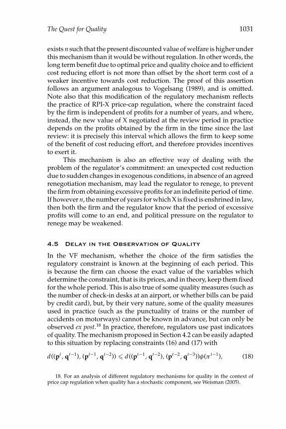
course is not limited to the case in hand, but it affects any policy aimedat influencing the quality of a firm’s supply, whether by a regulatorymechanism, or by the direct imposition of standards, in areas such asenvironmental standards, the quality level of public services such ashealth, education and police protection, health and safety regulationin food and durable goods, and in general any situation where thereare no market prices which signal the marginal users’ willingnessto pay. Conceptually, this is due to the fact that the social valuationof a quality change is determined by the marginal valuation of allconsumers purchasing a good, including the inframarginal ones, whosevaluation of quality changes is not revealed by the purchase decision.Nevertheless, relative to the policy of mandatory quality levels adoptedby some regulators, the dynamic regulatory mechanism proposed inProposition 3 has considerably lower information requirements, becauseit requires knowledge of the consumers’ valuation for departures fromthe existing quality levels, rather than knowledge of the consumers’valuation for a range of possible quality levels,13 and of the firm’s costfunction.

We begin the analysis of the long run property of the quality-adjusted VF mechanism with the study of a special case.

Proposition 2: Let the welfare function be quasi-convex. Let the regulatedfirm be subject in each period to the quality adjusted VF constraint, (11). Theprice-quality vector chosen by the firm converges to the price-quality vector(p∗, q∗).

Thus, if the welfare function is quasi-convex, including qualityin the price cap in the way proposed in (11), which is the theoreticalcounterpart of the ad hoc mechanism used in practice by some regulators,is sufficient for the firm’s choices to tend to the second best. Thegeometric reason is that, exactly as in the VF mechanism (in whoseset-up the welfare function is quasi-convex), the hyperplane tangentto the isowelfare locus at a given point contains only points which are“welfare better” than that point. Therefore, welfare increases in everyperiod.

While, with fixed qualities, quasi-convexity of the welfare functionis a consequence of the natural assumption that the demand functionsbe decreasing, and is therefore realistic, when the consumers’ utilitydepends on both prices and qualities, it cannot be warranted. To see this,consider as an example the simplest possible case, with one good, and

13. For example, a survey trying to ascertain the former would ask a commuter howmuch more she would be willing to pay for her season ticket for, say, a reduction of thefrequency of late trains from 15 to 14 trips per year, rather than how much she would bewilling to pay for a season ticket with all possible frequencies of late trips.


FIGURE 2. THE POSSIBILITY OF THE REGULATORY CYCLES

a linear demand function where the coefficients depend on the qualityof the good:

x = a (q ) − b(q )p a (q ), b(q ), a ′(q ) > 0,b ′(q )b(q )

<a ′(q )a (q )

. (14)

Claim 1: Let the market demand be given by (14). The consumer’s surplusis quasi-convex if and only if b′(q) > 0.

Without quasi-convexity of the social welfare function, the half-space defined by constraint (11)—which is an upward shift of thehyperplane tangential to the isowelfare through the point chosen inthe previous period—contains points which are “welfare worse” thanthe previous period choice. In this case, the regulatory process maybackfire, converging to a cycle: the geometric example provided in Fig-ure 2 suffices to illustrate the point. As before, the isoprofit (isowelfare)loci are the solid (dashed) curves. Suppose the firm starts from pointA. Here the line aa is tangent to the isowelfare, and, because profit isstrictly positive, the constraint is shifted up, to, say, position a′a′. Withthis constraint, the firm will choose point B. Note that welfare is lowerat point B than at point A. At B, the isowelfare is tangent to line bb; profitat point B is higher than at A, and therefore strictly positive, and theconstraint is shifted up, say to position b′b′. From here the firm wouldchoose again point A, and the cycle is repeated. Note that, apart fromhaving positive profit, the cycle constituted by points A and B is such


that a Pareto improvement is possible: both the firm and the regulatorcan be made better off in each period if a different point were chosen.14

4.3 Ensuring Convergence of the Dynamic Priceand Quality Mechanism

Without quasi-convexity of the welfare function, convergence to so-cially optimal prices and quality requires additional constraints. Wepropose here one such constraint, which has the same informationrequirement as the quality-adjusted VF constraint studied in the pre-vious subsection. Loosely speaking, the additional constraint requiresthe firm to make choices in each period which are not too differentfrom the choices it made in the previous period. For this reason, it isnatural to name it the “distance constraint.” Imposing this constraint,in turn, requires a modification of the quality-adjusted VF constraint(11). To derive formally the distance constraint, we begin by definingthe following function: for a given vector of strictly positive weights(ρ1, . . . , ρn, ω1, . . . , ωm) ∈ R

n+m++ , and for a given vector of strictly posi-

tive parameters (ξ1, . . . , ξn, ζ1, . . . , ζm) ∈ Rn+m++ , given two price-quality

vectors (pA, qA) and (pB, qB), let their distance15 be given by

d((pA, qA), (pB, qB)) =n∑

i=1

ρi∣∣pA

i − pBi

∣∣ξi +m∑

j=1

ω j∣∣q A

j − q Bj

∣∣ζ j . (15)

The Distance Constraint. In each period, the firm must choose a price-quality vector satisfying:

d((pt , qt), (pt−1, qt−1)) � d((pt−1, qt−1), (pt−2, qt−2))φ(π t−1), (16)

where φ(π ) is any monotonic continuous function satisfying φ(0) = 1 andφ(π ) ∈ (0, 1) for every π �= 0.

The distance constraint requires that, except when the accountingprofit in the previous period is 0, the distance between the price-qualityvector chosen in one period and the price-quality vector chosen in the previousperiod must shrink with time. If on the other hand, today’s profit is 0, then

14. Vogelsang (1988) also identifies the possibility of cycles: in his paper, the regulatorymechanism transfers to the firm in each period the second order approximation of thechange in consumers’ surplus due to the change in the firm’s choices, and the firm canstrategically follow a cycle to increase its profit.

15. This is consistent both with the everyday use of the word “distance”, and withthe mathematical notion of distance on a cartesian space Rk as a function d fromR2k into R+, satisfying reflexivity (for every z ∈ Rk , d(z, z) = 0), symmetry, (for everyz, z′ ∈ Rk , d(z, z′) = d(z′, z)), and the Cauchy–Schwartz inequality (for every z, z′, z′′ ∈Rk , d(z, z′) + d(z′, z′′) � d(z, z′′)) (Kelley, 1955).


(16) requires that the distance between tomorrow’s choice and today’sbe no greater than the distance between today’s and yesterday’s choice.In other words, slightly less rigorously, prices and qualities must fallwithin an aggregate band, the width of which depends on the firm’sprevious choices; this corresponds loosely with the practice of someregulators to constrain some prices within certain limits. The role of thedistance constraint (16) is to ensure convergence of the price-qualitychoices of the firm: as shown above, without it, the mechanism may belocked in a Pareto inefficient cycle. Note also the weights ρi and ωj andthe parameters ξi and ζj are unrestricted. They could reflect the differentunits in which the firm’s choices are measured, or some assessmentof the relative importance of the different quality aspects, though thisis not necessary. Were the regulator not concerned with some prices orquality dimensions, the appropriate weights may be set arbitrarily closeto 0.

The distance constraint may however be too tight, in the sense ofmaking it impossible for a firm to satisfy it and obtain non negativeprofits. In this case, the quality-adjusted VF constraint (11) must bemodified.

The Modified Quality-Adjusted VF Constraint. In each period,the firm must choose a price-quality vector satisfying:

xt−1 · pt

xt−1 · pt−1 � 1 −(

π t−1

Rt−1 γ t − ut−1 · (qt − qt−1)Rt−1

), (17)

where ut−1 = (ut−11 , . . . , ut−1

m ) is given in (12).

The difference between (17) and the quality-adjusted VF constraint(11) is in the term γ t. This is defined by the following procedure: qualitiesare fixed at the previous period levels qt−1.

Step 1: Choose rt0. rt

0 is the value of r that solves the following equation:

d((x−1(rxt−1, qt−1), qt−1), (pt−1, qt−1))

= d((pt−1, qt−1), (pt−2, qt−2))φ(π t−1).

Step 2: Choose γ t0 . γ

t0 is the value of γ that solves the equation:

xt−1 · x−1(r t0xt−1, qt−1) = xt−1 · pt−1 − γπ t−1.

Step 3: Choose γ t. γ t = min{1, γ t0}.

When γ t = 1, the shift is the same as in VF, quality adjustmentapart. If γ t < 1, then the shift determines a less tight constraint. This isnecessary to ensure that, in each period, there exist allowed price-quality


FIGURE 3. THE DETERMINATION OF THE FACTOR γ

vectors which give the firm non negative profit, or else the firm wouldleave the market, at least for some discount rates.

Figure 3 shows the determination of the firm’s constraints in theone-good one-quality case: n = m = 1. Let A be the price-quality vectorchosen in period t − 1; point B is the price-quality vector where thequality-adjusted VF constraint (17) with qt = qt−1 and γ t = 1 holds as anequality. At point B, the firm at least breaks even, and, knowing that itwill also at least break even in every future period, is willing to remainin the market for every positive discount factor. This follows from theassumption of decreasing ray returns, as discussed above in the caseof fixed qualities (see the paragraph following (10)). If the mechanismto regulate quality were the exact analogue to the VF mechanism, thiswould be it: γ t would be 1, and the firm would face only a constraintgiven by the parallel shift of the hyperplane tangent to the isowelfarefrom point A to point B, and could choose any point in the half-space tothe left of the shifted hyperplane (the grey area on panel (a)). However,as mentioned above, when quality varies, the distance constraint (16)(drawn as the ellipse centred in A in panel (a)) is also needed. With thisadditional constraint, the feasible region is only the darker region inpanel (a).

It may be the case that, as drawn in panel (a), point B belongs tothe feasible region, and so there is at least one point with non negativecurrent profits in the feasible area. In this case, imposing the quality-adjusted VF constraint (11) is sufficient. The distance constraint mayhowever be too demanding, as depicted in panel (b) in Figure 2, wherethe ellipse is smaller. In this case, if the hyperplane with slope (xt−1, ut−1)through point A were shifted all the way to point B, that is, if γ t were1, the admissible region would be empty. We therefore take γ t less than1 to stop the shift at point C: this is the point where, keeping qualities


constant, prices are changed in such a way to reduce proportionally allquantities so as to satisfy the distance constraint (16) as an equality. Thisensures that the firm’s feasible choice set is non empty: it is the dark areain panel (b). Moreover, at point C the firm’s profit is higher than at point Band so the firm can choose at least one price-quality vector giving non-negative profits in the present period and therefore ensuring that thefirm wants to stay in the market. Step 1 determines point C algebraically:rt

0 is the factor by which the output vector sold in t − 1 must be scaledup at time t to satisfy constraint (16) as an equality, when the qualitiesare the same as in period t − 1. Steps 2 and 3 simply ensure that if thepoint B is to right of C, then γ t is 1, and vice versa, if point C is to theright of B, then the shift is to the intersection of the distance constraintand the ray where quantities are reduced proportionally. Note that thedetermination of rt

0 and therefore of γ t requires only knowledge of theprevious period accounting profits and of the local demand conditions,and not of the firm’s cost function.

We can now show, in Proposition 3, that the mechanism constitutedby constraints (16) and (17) has the same long run properties of the VFmechanism: a profit maximising firm which is required to satisfy theseconstraints period after period, chooses price-quality vectors whichform a sequence converging16 to the zero-profit Ramsey price-qualityvector.17

Proposition 3: Let (pt, qt) be the price-quality vector chosen by a firmsubject in each period t to constraints (16) and (17). The sequence {(pt, qt)}∞t=1converges to the second best optimal price-quality vector (p∗, q∗).

Notice also that, just as the original, fixed quality VF mechanism,the mechanism defined by constraints (16) and (17) does not requireprofits to be non decreasing in each time period. While such a directconstraint would also ensure convergence to a second best optimalvector, it would run counter to another important regulatory objective,the provision of incentive for cost reduction, as it would be self-defeatingfor the firm to take advantage of cost reducing opportunities. We takeup this point in the next subsection.

16. In practice regulators and policy makers are also interested in the speed ofconvergence. This is a topic that has found relatively little attention in the literature:simple examples illustrate that it is very hard to obtain general conclusions on the matter,even in simple cases where qualities are fixed, because the process of convergence is highlysensitive to the starting point (see De Fraja and Iozzi, 2001).

17. As with VF, initial conditions are needed. If past data are missing or not suitable,the regulator can leave the firm unregulated in period 1, impose constraint (17) fromperiod 2 and constraint (16) from period 3.


To end this section, we note that if the regulatory process does notimpose convergence to the second best, that is to the point where profitis 0, then the distance constraint is not required: the quality-adjustedVF constraint (11) ensures that the firm’s choices converge to a pointwhere the isowelfare and the isoprofit are tangent. The reason is exactlythe same as in Brennan’s set-up (1989) as his argument does not use thequasi-convexity of the welfare function.

4.4 Endogenous Costs

The focus of the mechanism proposed in Section 4.2 is the provision ofincentives for the socially optimal prices and qualities, just as the VFmechanism focused on the socially optimal (Ramsey) prices, and thecost structure is assumed to be exogenously given. The policy relevantquestion therefore arises of the robustness of our mechanism to therelaxation of this hypothesis, especially because one of the goals of pricecap regulation in practice is the provision of incentives for the regulatedfirm to reduce its costs. Note that cost reduction is not an issue in thesteady state, where all profit opportunities are exploited, including thosederiving from cost reducing effort. However, as shown by Sappington(1980), a profit maximising, non myopic firm may forgo cost reducingopportunities, or even deliberately increase its costs wastefully, tobenefit from more relaxed regulation in the periods immediately afterthe current one. As a consequence, along the adjustment path, welfarecan be lower than it would be with no regulation.

Vogelsang (1989) addresses this point. He shows that the incentivefor cost reduction can be maintained along the adjustment path whenthe firm maximises the present discounted value of its future profits:in his extension of the VF mechanism, past profits affect the currentset of constraints faced by the regulated firm only every n periods.Vogelsang’s extension applies, mutatis mutandis, to the regulatory mech-anism proposed in Section 4.2. Specifically, to extend the mechanism tothis case, we may consider two types of periods. In “normal” periods,past profits are simply ignored: γ t is set to 0 in the quality-adjusted VFconstraint (17), and φ(πt) is set to 1 in the distance constraint (16). Everyn-th period, however, is a “review” period, during which the firm facesthe original constraints (16) and (17), where the measure of profit isgiven by average profits for the previous n periods, and where γ t is thelargest value which ensure that the choice set of the firm is not empty,with a procedure exactly analogous to the one described in Steps 1–3in Section 4.2. This mechanism ensures convergence to the second bestprice-quality vector and to the efficient choice of cost reducing effort.Moreover, for every value of the regulated firm’s discount factor, δ, there


exists n such that the present discounted value of welfare is higher underthis mechanism than it would be without regulation. In other words, thelong term benefit due to optimal price and quality choice and to efficientcost reducing effort is not more than offset by the short term cost of aweaker incentive towards cost reduction. The proof of this assertionfollows an argument analogous to Vogelsang (1989), and is omitted.Note also that this modification of the regulatory mechanism reflectsthe practice of RPI-X price-cap regulation, where the constraint facedby the firm is independent of profits for a number of years, and where,instead, the new value of X negotiated at the review period in practicedepends on the profits obtained by the firm in the time since the lastreview: it is precisely this interval which allows the firm to keep someof the benefit of cost reducing effort, and therefore provides incentivesto exert it.

This mechanism is also an effective way of dealing with theproblem of the regulator’s commitment: an unexpected cost reductiondue to sudden changes in exogenous conditions, in absence of an agreedrenegotiation mechanism, may lead the regulator to renege, to preventthe firm from obtaining excessive profits for an indefinite period of time.If however n, the number of years for which X is fixed is enshrined in law,then both the firm and the regulator know that the period of excessiveprofits will come to an end, and political pressure on the regulator torenege may be weakened.

4.5 Delay in the Observation of Quality

In the VF mechanism, whether the choice of the firm satisfies theregulatory constraint is known at the beginning of each period. Thisis because the firm can choose the exact value of the variables whichdetermine the constraint, that is its prices, and in theory, keep them fixedfor the whole period. This is also true of some quality measures (such asthe number of check-in desks at an airport, or whether bills can be paidby credit card), but, by their very nature, some of the quality measuresused in practice (such as the punctuality of trains or the number ofaccidents on motorways) cannot be known in advance, but can only beobserved ex post.18 In practice, therefore, regulators use past indicatorsof quality. The mechanism proposed in Section 4.2 can be easily adaptedto this situation by replacing constraints (16) and (17) with

d((pt , qt−1), (pt−1, qt−2)) � d((pt−1, qt−2), (pt−2, qt−3))φ(π t−1), (18)

18. For an analysis of different regulatory mechanisms for quality in the context ofprice cap regulation when quality has a stochastic component, see Weisman (2005).


and

xt−1 · pt

xt−1 · pt−1 � 1 −(

π t−1

Rt−1 γ t−1 − ut−1 · (qt−1 − qt−2)Rt−1

). (19)

The difference with constraints (16) and (17) is simply that all qualitymeasures are delayed by one period: qt−1 replaces qt, qt−2 replaces qt−1,and qt−3 replaces qt−2.

Proposition 4: Let (pt, qt) be the price-quality vector chosen by a firmsubject in each period t to constraints (16) and (17). The sequence {(pt, qt)}∞t=1converges to the second best optimal price-quality vector (p∗, q∗).

Convergence under our mechanism is therefore ensured also in theplausible case when quality is observed only ex post, and therefore thisneed not further diminish the applicability of our proposed mechanismin practice.

5. Concluding Remarks

In this paper we study regulation of quality. We consider a regulatorymechanism which extends the regulatory mechanism suggested by VFand its practical counterpart, RPI-X price cap, and it is based on the sameprinciple of delegating economic decisions to the firm: the firm can freelymake its choices on the economic variables under its control, subject toa constraint over their average value, with this constraint tighteningover time. In the VF mechanism, the tightening of the constraint in eachperiod is automatically determined by the rate of profit over sales in thepast period. In the practice of RPI-X price cap regulation, the extent bywhich the firm must reduce its average price is exogenously given by Xand negotiated with the regulator every few years.

In some cases, the average price level permitted to the firm, asdetermined by X, is made dependent also on the quality of the servicesprovided by the firm itself, and we study the theoretical foundation tothe relationship between the average price and the quality of the servicesprovided by the regulated firm, formalising the practice followed bysome regulators to let the factor X in the RPI-X price cap depend onquality improvements.

In the mechanism we consider here, the firm may exceed the valueof the index which would be allowed by the VF mechanism, if it increasesthe quality of its output: the regulated firm can “sell” higher qualityto consumers, to the extent allowed by its constraints; conversely, ofcourse, the firm can lower the quality of its output, but must “bribe”the consumers via lower average prices. Formally, a quality adjustmentterm is added to the X factor: this term is a weighted average of the


marginal effects of the quality changes on consumers’ welfare and itis not in any way dependent on the firm’s cost, typically unknown tothe regulator. In analogy to the RPI-X price cap and the VF mechanism,where the weight of each price in the price average is given by its socialmarginal valuation in the previous period, the weight of each qualitymeasure in the quality adjustment term added to the X factor is given bythe social marginal valuation of that dimension of quality in the previousperiod. In other words, just as prices are weighted by the previous periodoutput, which is the marginal surplus due to a price change, quality isweighted by the marginal surplus associated to a quality improvementin the last period. The important difference with the VF mechanism is,of course, that the latter is not automatically observed like the former.We also show that, when the regulator’s objective function is not quasi-convex, which is well possible when quality affects consumers’ utility,this correction of the VF mechanism may be counterproductive: theregulated firm’s choices may be locked in a Pareto inefficient cycle.An additional requirement, that the firm’s choices are constrained tolie with an “aggregate price-quality band”, does address this problem.Formally, the firm is constrained to choose, in each period, qualities andprices satisfying two constraints: the modified quality-adjusted Vogelsang–Finsinger constraint, given by (17), and the distance constraint, (16).

The mechanism we consider allows the regulator to offer the firma formula with which quality changes can be valued, thus avoiding boththe need of regular negotiations on the weights of the quality measures,and the uncertainty associated with this bargaining process. While notbased on fully observable magnitudes like the VF mechanism for goodsand services where quality does not vary, it is a mechanism informa-tionally considerably less demanding than schemes such as minimumquality standards, which, to be set optimally, require knowledge of thefirm’s cost function and of the consumers’ valuations of a wide range ofpossible quality levels.

Appendix

Proof of Proposition 1. Consider the second best price-quality vector(p∗, q∗). This is the solution to the following problem:

maxp,q

v(p, q) s.t.: π (p, q) � 0. (A1)

The FOC to problem (20) are

∂L∂pi

= ∂v(p∗, q∗)∂pi

− µ∂π (p∗, q∗)

∂pi= 0 i = 1, . . . , n; (A2)


∂L∂q j

= ∂v(p∗, q∗)∂q j

− µ∂π (p∗, q∗)

∂q j= 0 j = 1, . . . , m. (A3)

where µ is the Lagrangean multiplier associated with the constraint in(A1). Because the unregulated firm can always make strictly positiveprofits, the social optimum is not the profit maximising vector, andbecause ∂v(p∗,q∗)

∂pi< 0 whenever ∂π (p∗,q∗)

∂pi> 0, µ is strictly positive, and

so the non negativity constraint holds as an equality: π (p, q) = 0. UseRoy’s identity, (2), and (6) in (A2), and substitute (7) into (A3), to write(A2) and (A3) as:

∂π (p∗, q∗)∂pi

= wi

µi = 1, . . . , n,

∂π (p∗, q∗)∂q j

= u j

µj = 1, . . . , m.

Now consider the problem of a profit maximizing firm subject to a reg-ulatory constraint given by (4). Note that, when deciding today’s price-quality vector, the firm takes the optimised value of future profits asgiven, and, because the price cap is static and there are no intertemporalconsumption effects, it maximises current profit:

maxp,q

π (p, q) s.t.: w · p − u · q ≤ I . (A4)

Let p and q be the solutions to this problem. They satisfy:

∂L∂pi

= ∂π (p, q)∂ pi

+ νwi = 0, i = 1, . . . , n; (A5)

∂L∂q j

= ∂π (p, q)∂ q j

− νu j = 0, i = 1, . . . , m. (A6)

Again, because profit increases in at least one price or decreases in at leastone quality, ν, the Lagrangean multiplier, is strictly positive. Therefore,at the solution of problems (A1) and (A4), the gradients of the profitfunction are proportional. This, combined with the fact that the firmobtains zero profit in both problems, implies (p∗, q∗) = (p, q). �Proof of Proposition 2. The proof is an extension of the proof givenby VF for their Proposition 1, to the case when quality also adjusts.Consider the set �0 = {(p, q) | π (p, q) � 0}: this is the set of price-qualityvectors giving non negative profit. This set is compact because revenuesare finite at any price vector. An argument analogous to the proof ofLemma 1 in Proposition 3 shows that when the feasible region forthe firm is given by (17), there are points giving positive profit, or, inother words, the sequence {(pt, qt)}∞t=1 is in �0. We now show that the


sequence {v(pt, qt)}∞t=1 is monotonic and therefore that it has a uniqueaccumulation point in �0. The quasi-convexity of v(p, q) implies that

v(pt , qt) − v(pt−1, qt−1) � �v(pt−1, qt−1)

[pt − pt−1

qt − qt−1

], (A7)

where �v(pt−1, qt−1) is the gradient of the function v at (pt−1, qt−1). Thissatisfies �v(pt−1, qt−1) = (−xt−1, ut−1). Multiplying through the r.h.s.,(A7) can be rewritten as:

v(pt , qt) − v(pt−1, qt−1) � −xt−1 · (pt − pt−1) + ut−1 · (qt − qt−1). (A8)

Next note that (17) can be written as −xt−1 · (pt − pt−1) + ut−1 ·(qt − qt−1) � π t−1, and therefore (A8) implies v(pt, qt) − v(pt−1, qt−1) �π t−1 � 0. This shows that the sequence {v(pt, qt)}∞t=1 is monotonic andtherefore it converges. Moreover, we have

0 = limt→∞[v(pt , qt) − v(pt−1, qt−1)] � lim

t→∞ π t−1,

and, so in the limit, the firm makes zero profit. All there remains toshow is that the firm’s choice converges to a second best optimum.This is identical to Step 3 in VF (p. 164): if (p, q) is the accumula-tion point of the sequence {(pt, qt)}∞t=1, then the surfaces {v(p, q) | v =v(p, q)}, {π (p, q) | π = π (p, q) = 0}, and the constraint are all tangent toeach other. Finally, if the sequence {(pt, qt)}∞t=1 does not converge, thenthe argument used in Iozzi et al. (2002, Proposition 2a, p. 113) showsthat the limit points of any convergent subsequence of the sequence{(pt, qt)}∞t=1 must satisfy all the first order conditions for a second bestoptimum. �Proof of Claim 1. Notice first of all that, in this simple one good set-up, convexity of consumers’ surplus is equivalent to convexity of theisowelfare curves in the (p, q)-cartesian plane, d2q

dp2 > 0. With this obser-vation, the proof is straightforward algebra. Start from the expressionfor consumers’ surplus:

v(p, q ) =∫ a (q )

b(q )

p[a (q ) − b(q )z] dz = b(q )

2

(a (q )b(q )

− p)2

.

The isowelfare curve has slope:

dqdp

= −∂v/∂p∂v/∂q

= b(q )

a ′(q ) − b ′(q )2

(a (q )b(q )

+ p) ,

which is positive if b′(q )b(q ) <

a ′(q )a (q ) as posited. From the above:


d2qdp2 = ∂

∂p

b(q )

a ′(q ) − b ′(q )2

(a (q )b(q )

+ p) = b(q )b ′(q )

2(

a ′(q ) − b ′(q )2

(a (q )b(q )

+ p))2 ,

after rearrangement, which establishes the statement. �Proof of Proposition 3. We first show that the mechanism is well defined,and then we establish its convergence properties. Begin by noting thatthe firm’s problem is a standard dynamic programming problem (e.g.,Stokey and Lucas, 1989, p. 66). To see this, introduce two vectors ofauxiliary variables, pt

P and qtP, which are the previous periods price

and quality vectors: ptP = pt−1, and qt

P = qt−1 (the subscript P stands forprevious). Now write the firm’s problem as

max{(pt ,qt ,pt

P ,qtP

)}∞t=1

∞∑t=1

δt−1π (pt , qt)

s.t.:(pt , qt , pt

P , qtP

) ∈ �(pt−1, qt−1, pt−1

P , qt−1P

), t = 1, 2, . . . ,(

p0, q0, p0P , q0

P

) ∈ Rm × Q × R

m × Q given. (A9)

We have followed the same notation as Stokey and Lucas: the set � isthe set of admissible values of the vector (pt, qt, pt

P, qtP) given that it

took value (pt−1, qt−1, pt−1P , qt−1

P ) in the previous period. In our problem� is the set is given by the vectors which satisfy (17), the rewriting ofconstraint (16) in the present notation:

d((pt , qt), (pt−1, qt−1)) � d((pt−1, qt−1),

(pt−1

P , qt−1P

))φ(π t−1),

and the definitional constraints,

ptP = pt−1,

qtP = qt−1.

By construction the set � is non empty, and the firm’s problem (A9) hasa solution, which is the solution of a functional equation (Stokey andLucas, 1989, Theorem 4.3, pp. 72–73):

ψ(p, q, pP , qP ) = max(p,q,pP ,qP )∈�(p,q,pP ,qP )

[π (p, q) + δψ(p, q, pP , qP )],

and could, in principle, be found with numerical methods. The focusof the Proposition, however, is on the convergence properties of themechanism, and we turn to these in the rest of the proof. We proceedalong the following steps:

Lemma 1: π t � 0 for every t > 0.


Proof . We need to show that there exists at least one feasible price-quality vector which allows the firm to make non negative profits inthe current period, and hence in every future period. This is sufficient—though not necessary—to ensure that the present value of future profitsis non negative in every period. Let rt

V be defined as the smallest valueof r ≥ 1 that solves the following equation:

xt−1 · x−1(rxt−1, qt−1) = xt−1 · pt−1 − π t−1. (A10)

Define r t = r tV if γ t = 1 and r t = r t

0 if γ t < 1. Let the firm, in period t,choose qualities qt−1, and prices x−1(r txt−1, qt−1).

Rewrite constraint (17) as

xt−1 · pt � xt−1 · pt−1 − (π t−1γ − ut−1 · (qt − qt−1)). (A11)

Given that the firms has not changed its quality choices relatively totime t − 1, the definitions of rt

V in (A10) and of rt0 in Step 1, and the way

in which γ t is derived, constraint (A11) can be rewritten as

xt−1 · x−1(r txt−1, qt−1) = xt−1 · pt−1 − γπ t−1,

from which it follows that

xt−1 · x−1(r txt−1, qt−1) = xt−1 · pt−1 − π t−1 + (1 − γ t)π t−1,

xt−1 · x−1(r txt−1, qt−1) = C(xt−1, qt−1) + (1 − γ t)π t−1,

r txt−1 · x−1(r txt−1, qt−1) = r tC(xt−1, qt−1) + r t(1 − γ t)π t−1,

r txt−1 · x−1(r txt−1, qt−1) � C(r txt−1, qt−1) + r t(1 − γ t)π t−1.

The last line follows from the assumption of decreasing (quantity) rayaverage costs. Rearranging,

r txt−1 · x−1(r txt−1, qt−1) − C(r txt−1, qt−1) � r t(1 − γ t)π t−1 � 0.

In the above, the LHS is the profit obtained by the firm when it offers thevector r txt−1. The second inequality follows from the fact that γ t ∈ [0, 1].This proves that the vector r txt−1 gives non negative profits. The wayin which r t is defined ensures that this price-quality vector is always inthe firm’s allowed region. �

Next consider the sequence {(pt, qt)}∞t=1 of the firm’s choices. Fort = 1, 2, . . . , define dt ∈ R+ as d((pt, qt), (pt−1, qt−1)). By (16), dt+1 � dt,and therefore {dt}∞t=1 converges to a point, say d∞. If d∞ = 0, then thesequence {(pt, qt)}∞t=1 of the firm’s choices has converged to a point (p, q)which must yield zero profit: to see this, note that, just as in VF, themodified quality-adjusted VF constraint, (17), is shifted when profit ispositive in such a way to prevent the firm from choosing the same vector


in the next period, against the hypothesis that the firm’s choice hasconverged to (p, q). If instead d∞ > 0, then the firm’s choices in thelimit are on a path of equidistant points (which may or may not be acycle); it must be the case that the profit at any of these points is zero,otherwise the firm would be compelled by the distance constraint (16) toreduce the distance between subsequent points, against the assumptionof convergence to d∞ > 0.

To continue with the argument, consider the following problem:

maxpt ,qt

π (pt , qt) s.t.: x · pt − u · qt � C(x, q) − u · q, (A12)

where (p, q) is any point on the limit sequence of the firm’s choices, andwhere x = (x1, . . . , xn) and u = (u1, . . . , un). This is the problem obtainedfrom the original problem by ignoring the distance constraint (16), thatis by imposing only (11). Denote with pt and qt the solution to problem(A12). This satisfies the following first-order conditions:

∂π (pt , qt)∂ pt

i= λxi for all i = 1, . . . , n;

∂π (pt , qt)∂ q t

i= λu j for all j = 1, . . . , m;

where λ is the Lagrangean multiplier associated with the constraintin (A12). We must have that, as in Step 3 in VF (p 164), the sur-faces {v(p, q ) | v = v(p, q)}, {π (p, q ) | π = π (pt , qt)}, and the constraintin (A12) are all tangent to each other, and therefore the next periodproblem for the firm is given by (A12) again (because the quality-adjusted VF constraint is unchanged). This implies, incidentally, that allthe firm’s choice in the limit sequence lie on the same hyperplane. Notealso that at the solution (pt , qt) of problem (A12), the distance constraint(16) is satisfied, and therefore the solution to (A12) is the same as thesolution to (A12) with the added (16). Finally, because π (p, q) = 0 asshown above, Proposition 3 is established. �

Proof of Proposition 4. The proof is essentially identical to the proof ofProposition 3, and is omitted. �

References

AEEG, 1999, Decision n. 202/99: Decision concerning the regulation of the levels of the quality ofservices as related to the unplanned interruption of the energy supply, law n. 481, 14 November1995, art. 2(2). Italian Gas and Electricity Authority, Milan.

——, 2000, Decision 237/2000: Criteria to determine the tariffs for gas distribution and supply tothe customers of the captive market. Italian Gas and Electricity Authority, Milan.


——, 2004, Decision n.4/04: Comprehensive listing of the decisions of the Italian Gas andElectricity Authority on the regulation of the quality of distribution, measurement and supplyof electricity, 2004–2007. Italian Gas and Electricity Authority, Milan.

Armstrong, M. and D.E.M. Sappington, 2005, “Recent Developments in the Theory ofRegulation,” in M. Armstrong and R. Porter, eds., Handbook of Industrial Organization,vol. III. New York and Amsterdam: North-Holland.

——, S. Cowan, and J. Vickers, 1994, Regulatory Reform: Economic Analysis and BritishExperience. MA, Cambridge: MIT Press.

Banerjee, A., 2003, “Does Incentive Regulation ‘Cause’ Degradation of Retail TelephoneService Quality?” Information Economics and Policy, 15, 243–269.

Baron, D.P. and R.B. Myerson, 1982, “Regulating a Monopolist with Unknown Cost,”Econometrica, 50, 911–930.

Beil, R.O., D.L. Kaserman, and J.M. Ford, 1995, “Entry and Product Quality Under PriceRegulation,” Review of Industrial Organization, 10, 361–372.

Bertazzi, A., E. Fumagalli, and L. Lo Schiavo, 2005, The use of customer outage cost surveysin policy decision-making: The Italian experience in regulating quality of electricity supply.Proceedings of 18th International Conference & Exhibition on Electricity Distribution2005, Turin, Italy.

Bos, D., 1981, Economic Theory of Public Enterprise. Berlin: Springer-Verlag.Bradley, I. and C. Price, 1988, “The Economic Regulation of Private Industries by Price

Constraints,” Journal of Industrial Economics, 37, 99–106.Brekke, K.R., R. Nuscheler, and O.R. Straume, 2006, “Quality and Location Choices Under

Price Regulation,” Journal of Economics & Management Strategy, 15, 207–227.Brennan, T.J., 1989, “Regulating by Capping Prices,” Journal of Regulatory Economics, 1,

133–147.De Fraja, G. and A. Iozzi, 2001, “Short-term and Long-term Properties of Price Cap

Regulation,” International Journal of Development Planning Literature, 16, 51–60.Feldstein, M., 1972, “Distributional Equity and the Optimal Structure of Public Prices,”

American Economic Review, 62, 32–36.Gabszewicz, J.J. and J.F. Thisse, 1979, “Price Competition, Quality and Income Disparities,”

Journal of Economic Theory, 20, 340–359.Iozzi, A., 2002, “La riforma della regolazione nel settore autostradale,” Economia Pubblica,

32, 71–93.——, J.A. Poritz, and E. Valentini, 2002, “Social Preferences and Price Cap Regulation,”

Journal of Public Economic Theory, 4, 95–114.Kelley, J.L., 1955, General Topology. Amsterdam: D. van Nostrand Company.Laffont, J.-J., 1994, “The New Economics of Regulation Ten Years After,” Econometrica, 62,

507–537.—— and J. Tirole, 1991, “Provision of Quality and Power of Incentive Schemes in

Regulated Industries,” in J.J. Gabszewicz and A. Mas-Colell, eds., Equilibrium Theoryand Applications, pp. 137–156. Cambridge, UK: Cambridge University Press.

—— and ——, 1996, “Creating Competition Through Interconnection: Theory and Prac-tice,” Journal of Regulatory Economics, 10, 227–257.

Lo Schiavo, L., R. Malaman, and F. Villa, 2005, Continuity of electricity supply regulationdriven by economic incentives: does it work? the Italian experience. Proceedings of 18thInternational Conference and Exhibition on Electricity Distribution, Turin, Italy.

Ma, C.-A. and J.F. Burgess, Jr. 1993, “Quality Competition, Welfare, and Regulation,”Journal of Economics, 58, 153–173.

MORI, 2002, The 2004 Periodic Review: Research into Customers’ Views.Mussa, M. and S. Rosen, 1978, “Monopoly and Product Quality,” Journal of Economic

Theory, 18(2), 301–317.


NMPRC, 2002, Annual Report 2002. Santa Fe, NM: New Mexico Public Regulation Com-mission.

Oates, W.E. and P.R. Portney, 2003, “The Political Economy of Environmental Policy,”in K.-G. Maler and J. Vincent, eds., Handbook of Environmental Economics, Chap. 8.Amsterdam: North-Holland/Elsevier Science.

OFGEM, 2001a, Guaranteed and Overall Standards of Performance: Final Proposals. London:OFGEM.

——, 2001b, Information and Incentives Project. Incentive Schemes: Final Proposals. London:OFGEM.

——, 2003, Electricity Distribution Price Control Review. Initial Consultation. London:OFGEM.

OFWAT, 1999, Future Water and Sewerage Charges 2000–2005: Final Determinations. London:OFWAT.

——, 2002, Linking Service Levels to Prices. London: OFWAT.Resende, M. and L.O. Facanha, 2005, “Price-Cap Regulation and Service-Quality in

Telecommunications: An Empirical Study,” Information Economics and Policy, 17, 1–12.Rovizzi, L. and D. Thompson, 1992, “The Regulation of Product Quality in the Public

Utilities and the Citizen’s Charter,” Fiscal Studies, 13, 74–95.Samdal, K., G. Kjølle, B. Singh, and F. Trengereid, 2002, Customers’ Interruption Costs—

What’s the Problem? Technical Reports of 17th International Conference & Exhibitionon Electricity Distribution, Barcelona, Spain.

Sappington, D.E.M., 1980, “Strategic Firm Behavior Under a Dynamic Regulatory Adjust-ment Process,” Bell Journal of Economics, 11, 360–372.

——, 2003, “The Effects of Incentive Regulation on Retail Telephone Service Quality inthe United States,” Review of Network Economics, 2(4), 355–375.

——, 2005, “Regulating Service Quality: A Survey,” Journal of Regulatory Economics, 27(2),123–154.

—— and D.S. Sibley, 1988, “Regulating Without Cost Information: The IncrementalSurplus Subsidy Scheme,” International Economic Review, 29(2), 297–306.

Shaked, A. and J. Sutton, 1982, “Relaxing Price Competition Through Product Differenti-ation,” Review of Economic Studies, 49, 3–14.

Sheshinski, E., 1976, “Price, Quality and Quantity Regulation in Monopoly Situations,”Economica, 43, 127–137.

Spence, M., 1975, “Monopoly, Quality and Regulation,” Bell Journal of Economics, 6, 417–429.

Stigler, G.J., 1971, “The Theory of Economic Regulation,” Bell Journal of Economics, 2, 3–21.Stokey, N.L. and R.E. Lucas, 1989, Recursive Methods in Economic Dynamics. Cambridge,

MA: Harvard University Press.Trengereid, F., 2003, Quality of Supply Regulation in Norway. Proceedings of 17th Interna-

tional Conference & Exhibition on Electricity Distribution, Barcelona, Spain.Vogelsang, I., 1988, “A Little Paradox in the Design of Regulatory Mechanisms,” Interna-

tional Economic Review, 29(3), 467–476.——, 1989, “Price Cap Regulation of Telecommunications Services: A Long Run Ap-

proach,” in M.A. Crew, ed., Deregulation and Diversification of Utilities, pp. 21–42. Boston:Kluwer.

—— and J. Finsinger, 1979, “A Regulatory Adjustment Process for Optimal Pricing byMultiproduct Monopoly Firms,” Bell Journal of Economics, 10, 157–171.

Waddams Price, C., B. Brigham, and L. Fitzgerald, 2002, Service quality in regulatedmonopolies. Center for Competition and Regulation, University of East Anglia, WorkingPaper 02-4.

Weisman, D.L., 2005, “Price Regulation and Quality,” Information Economics and Policy, 17,165–174.

The Quest for Quality: A Quality Adjusted Dynamic Regulatory Mechanism

Documents

Transcript of The Quest for Quality: A Quality Adjusted Dynamic Regulatory Mechanism