WATER RESOURCES RESEARCH, VOL. 20, NO. 10, PAGES 1453-1465, OCTOBER 1984

A Spectral Theory of Rainfall Intensity at the Meso-/ Scale

ED WAYMIRE

Department of Mathematics, Oregon State University, Corvallis

VIJAY K. GUPTA

Department of Civil Engineering, University of Mississippi, University

IGNACIO RODRIGUEZ-ITURBE

Universidad Simon Bolivar, Caracas, Venezuela

The available empirical descriptions of extratropical cyclonic storms are employed to formulate a physically realistic stochastic representation of the ground level rainfall intensity field in space and time. The stochastic representation is based on three-component stochastic point processes which possess the general features of the embedding of rain cells within small mesoscale areas within large mesoscale areas within synoptic storms. Certain scale idealizations, and assumptions on functional forms which qualita- tively reflect the physical features, lead to a closed form expression for the covariance function, i.e., the' real space-time spectrum, of the rainfall intensity field. The theoretical spectrum explains the empirical spectral features observed by Zawadzki almost a decade ago. Of particular interest and importance in this connection is an explanation of the empirical observation that the Taylorian propogation of the fine scale structure, via a transformation of time to space through the storm velocity, holds only for a small time lag and not throughout. The results here indicate the extent of this lag in terms of the characteristic scales associated with cell durations, cellular birthrates and velocities, etc.

INTRODUCTION

The increasingly detailed classification and description of observed features of various types of storms are gradually leading to a clearer physical picture of rainfall structure at the meso-fi scale (20-200 km) and meso-7 scale (1-20 km) (see, for example, Hobbs and Locatelli [1978], Harrold and Austin [1974], and Austin and Houze [1972]); here we have adopted the scale classification given by Orlanski [1975]. This structure shows that in general, a precipitation area of a given scale has one or several smaller-scale areas of more intense precipitation embedded within it. This observed preferred organization in rainfall structure constitutes the physical basis along which it is possible to investigate the statistical fluctuations in space- time rainfall intensity at the ground level. This article presents one such statistical study which is based on the observed rain- fall structure for extratropical cyclonic storms.

The approach presented here attempts to capture the gener- al picture of the preferred organization in rainfall structure in mathematical terms, i.e., that of a system of rain cells in space and time embedded within the hierarchy of a system of small mesoscale areas (SMSA) at the meso-7 scale embedded within a system of rainbands at the meso-fi scale which, in turn, are embedded within the synoptic disturbances at the meso-• scale (200-2000 km). A brief discussion of these features is given in section 2. The probabilistic assumptions on these features are stated in section 3. They lead to a mathematical representation of the rainfall intensity at the ground level. Even though the mathematical conditions are only intended to represent the observed physical structures in an approxi- mate manner, they are still too general for obtaining statistical information about the rainfall intensity field. Consequently,

Copyright 1984 by the American Geophysical Union.

Paper number 4W0839. 0043-1397/84/004W-0839505.00

three types of approximations are introduced for this purpose in section 4. The first type of approximation consists of as- signing specific mathematical forms to the stochastic processes in section 3. For example, the temporal occurrences of rain- bands over a specific geographic region are assumed to follow a Poisson process. This type of an approximation is invoked in the spirit of capturing only the "first-order properties" with regard to the various interactions and statistical dependencies that may exist in the occurrences of rainbands. The second type of simplification is the scale idealization in which, for example, a convective rainfall cell is represented as the oc- currence of a "point" in an SMSA. The rainfall due to a cell is then "spread" around this point by a suitable transformation. The third type of approximation involves the specific math- ematical forms given to various functions. The choice is based on capturing the qualitative behavior of these functions and getting closed form expressions. The general mathematical representation itself will allow for any choice of functional forms compatible with the physical structure. For example, in the case of the precipitation intensity at a point at a distance r from the center of a cell of age a it is assumed that intensity io at the center is maximum and decreases radially outward in space. To get closed form expressions, we then specialize to functional forms of the type proportional to i o exp {-•a} exp {-r2/2D2}, where •- • may be viewed as a measure of the life span of a cell and 2nD2of its spatial extent.

The assumptions introduced in sections 3 and 4 on the component stochastic processes of space-time rainfall are suf- ficient to specify its probability generating functional (pgfi) (see, for example, Waymire and Gupta [1981a, hi). In principle, once the pgfi is known, it is possible to compute the probabil- ities of extremes, of crossings, and of the space-time averages of the rainfall intensity field and the moments of this field. In practice, these types of computations involve nontrivial diffi- culties. In this article we have elected to study only the first

1453

1454 WAYMIRE ET AL.: THEORY OF RAINFALL INTENSITY

two moments of the space-time rainfall field. The moment computations employ the important concept of product den- sities as an indirect computation of the pgfl. Our interest in the spectrum or the covariance of the rainfall intensity is to a large extent motivated by an attempt to explain the empirical results of Zawadzki [1973] on the rainfall covariance. How- ever, in diverse hydrologic studies ranging from the design of rain gage networks [Rodriguez-lturbe and Mejia, 1974] to physically based statistical analysis of streamflows (see, for example, Waymire and Gupta [1981b]), a knowledge of the space-time rainfall spectrum plays an important role. Hereto- fore, since no physically based expressions of the rainfall spec- trum have been available in the literature, the selection of such expressions has been made on an ad hoc and restrictive basis (see, for example, Bras and Rodriguez-lturbe [1976]).

Closed form expressions for the mean and the covariance functions of the rainfall field are derived in sections 5 and 6.

An important consequence of these results is that the empiri- cal findings of Zawadzki [1973, Figure 15] can be theoretically explained on their basis. The highlights of these empirical find- ings are that when the cells' velocities relative to that of the rainband are zero, then the covariance function satisfies Taylor's hypothesis on fluid turbulence for time lags smaller than a-•, the mean life span of the cells. Taylor's hypothesis breaks down for time lags larger than a-•. A theoretical ex- planation of these findings is given in section 7. This article is concluded in section 8 with a brief discussion of directions for further research.

The mathematical analysis for computing the covariance in section 6 is not entirely elementary even though the purely technical aspects have been relegated to appendices, so it is suggested that this section be skipped on first reading. This does not interfere with the theoretical explanation of Za- wadzki's results given in section 7.

2. Ex•^•oPic^n C¾CnONIC SzoaM FE^zum•s

Extratropical cyclones, i.e., low-pressure systems, are a major source of precipitation in the mid-latitudes. The synop- tic features of such a storm at the meso-• scale are represented by the large systems of fronts curving outward from the storms' centers.

Various quantitative aspects of the storm system, such as shape, size, intensity, and lifetime, at various scales are tied to the nature of the air motions producing the precipitation. The main influx of moisture in the synoptic scale precipitation fields of extratropical cyclonic storms is attributed to the so- called "conveyor belt" flow which occurs upward from near the ground [see Hartold, 1973]. However, since the synoptic scale precipitation fields contain strikingly distinct substruc- tures, it is apparent that other locally dominant air motions are present. While the precise nature of the physical laws as- sociated with these various air motions is not available, the substructure is nonetheless observable in the form of smaller-

scale precipitation patterns embedded within the synoptic scale precipitation areas. We shall describe a few of these fea- tures as we proceed in order to facilitate some understanding of the patterns observed. Such an understanding is especially important for proper interpretation of the probabilistic con- struction to be described in the next section. For example, it is often stated in the atmospheric science literature that cells of heavy rainfall are observed to occur in compact groups rather than being randomly scattered; see Hartold and Austin [1974] or Houze [1981]. From a probabilistic point of view this means that cells are not independently distributed throughout

the large-scale field. Rather there is some physical interaction, perhaps in the form of updraft-downdraft mechanisms linked to the life cycles of the cells, which will be reflected in strong local statistical dependencies among cell occurrences as clus- ters. Since the physical mechanisms underlying these interac- tions are not understood in detail, it is not possible to specify the exact nature of these dependencies. Therefore certain first- order idealizations regarding statistical dependencies are in- voked in this article to cover such occurrences as clusters of cells.

The large-scale precipitation fields associated with fronts are attributed to a general stratiform precipitation mechanism. That is to say, the vertical air motions in the "frontal precipi- tation regions" are weak enough that the precipitation parti- cles readily fall upon formation aloft. These large-scale frontal precipitation regions move with the synoptic scale systems with lifetimes equal to that of the synoptic scale system.

Within the frontal rain areas are embedded regions of higher rainfall intensity called "rainbands" which range from 103 to 10 '• km 2. The rainfall in these regions is intensified according to some dominant airflow mechanism within the frontal precipitation area. The physical mechanisms at this scale are the least understood and depend on the type of frontal region in which they occur. So, while higher-intensity rainfall is characteristic of the various types of rainbands, there are further classifications in the forms of "warm frontal," "wide cold frontal," "surge," and "narrow cold frontal" rain- bands. The air motions within the warm frontal rainbands, for example, lead to a stratiform precipitation mechanism more intense than that in the larger-scale warm frontal precipitation field. On the other hand, the narrow cold frontal rainband is a consequence of a convective precipitation mechanism em- bedded within the stratiform precipitation field of the cold front. The wide cold frontal, warm frontal, and surge rain- bands are structurally similar but differ in their orientations. The air motions responsible for the narrow cold frontal rain- bands lead to a structure quite different in appearance from that of the others; see Houze [ 1981] for specific illustrations.

Rainbands are also observed to occur outside the frontal

precipitation areas as well. The pre-cold frontal (warm sector) bands are somewhat similar in structure to squall lines, though vertical air motions are somewhat greater in the well- developed squall lines and, consequently, precipitation rates are higher as well. The mechanisms which determine the orientations of bands outside the frontal precipitation areas are not understood.

The smallest precipitation element observable by radar is referred to as a "cell." Cells are represented by small, intense radar echoes of areas of the order of 10-50 km 2. While cellular

rainfall intensities need not be high except relative to the background precipitation, heavy rainfall fields are most often cellular. The warm frontal, wide cold frontal, and surge rain- bands each have a cellular structure.

Individual cells and certain clusters of cells within rainbands

are supported by identifiable regions of precipitation smaller than rainbands. These regions are classified as SMSA's by Austin and Houze [1972, p. 933]. Each SMSA within a rain- band is termed a "cluster potential region" by Gupta and Way- mire [1979] and is conceptualized to support a cluster of cells having one or more cells in it. The density of cells within each SMSA can be rather small though. We note here with interest that clouds are generally observed to occur in clusters or groups even in nonprecipitating cumulus cloud fields (see, for example, Lopez [1976] and Cho [1978]). One can think of

WAYMIRE ET AL.: THEORY OF RAINFALL INTENSITY 1455

TABLE 1. A Summary of the Observed Rainfall Structure in a Typical Extratropical Cyclonic Storm

Extratropical Cyclone Storm Structure Systems Frontal Precipitation Cluster Potential Characteristics (Synoptic) Areas or Rainbands (SMSA) Rain Cells

Horizontal > 10 '• 103-10 '• 10-103 10-50 spatial scale, km 2

Duration scale, > 12 1.5-4 0.5-4 0.7 hours

Air motions stratiform stratiform convective convective

Shape concave concave irregular convex Precipitation 0.5 4 8 10-100

intensity, mm/h

Motion from east in with fronts same as cells with wind at northern midcell

hemispheres level

Numbers are only intended as rough indications of orders of magnitude.

each cloud group as comprising a cluster potential region. Theoretical speculation with regard to the air motions associ- ated with cellular and SMSA precipitation fields is given by Austin and Houze [1972]. The mechanisms supporting the ex- istence of identifiable SMSA regions and of cells appear to be interlinked. It is supposed that the tendency for the cells to occur in clusters is perhaps due to a compensation of the downdraft in a precipitating cloud by an upward air motion in its vicinity. This upward motion gives an impulse to the neigh- boring warm air with the result that a new cell is born in the vicinity of a precipitating cell [Petterssen, 1956, p. 161]. Al- though it seems that the density of cells within an SMSA should be related to the spread of particles aloft, this is some- what ambiguous. Equally ambiguous is the effect of residual precipitation particles left aloft at the death of a cell and on the birth of new cells in the vicinity. A summary of the ob- served features of the rainfall patterns in a typical extratropi- cal cyclonic storm is given in Table 1. This summary is com- piled from various references given above.

3. MATHEMATICAL REPRESENTATION OF RAINFALL

INTENSITY FIELD

The mathematical representation given in this section is an extension and a generalization of the previous work by Gupta and Waymire [1979] to allow for temporal occurrences of multiple rainbands over a fixed but arbitrary geographic region. Physically, these occurrences can be due to a single synoptic scale disturbance passing over that region or to dis- tinct synoptic fronts.

In this article the term "stochastic point process" designates the random occurrences of events in a one- or higher- dimensional space; recall that the word "random" does not refer to uniform and independent occurrences. Each oc- currence is geometrically represented by a point in this space. For example, the random cell occurrences in space-time are denoted by the vector (z, y), where z • (-c•, c•) denotes the time of birth of a cell and y e R 2 denotes its spatial location at the time of birth. If B is a subregion of this three-dimensional space, then by a stochastic point process X( ) we also mean that X(B) is the random number of cells in the subregion B. Mathematically, the two modes of characterizing a point pro- cess, either by the coordinates of occurrences of random events or by the random number of such occurrences in one or more subregions, are equivalent; see Waymire and Gupta [1981a-I for a further discussion.

Fix a spatial origin at some geographic location within the range of extratropical storm systems. The locations of rain- bands are identified relative to this spatial origin, and the times at which rainbands arrive are measured with respect to a fixed but arbitrary time origin. The mathematical notations and assumptions will now be introduced.

Assumption l : Rainband Arrivals

The arrival times of rainbands, denoted by ..., s_ 2, s_ 1, So, sa, --. represent the random occurrence of a stochastic point process M( ) in the time interval (-c•, c•).

We shall use ps•(a)(s) ds to denote probability of a rainband arrival in time s to s + ds. Similarly, ps•(2)(sa, s2) ds• ds2 shall denote the probability of rainband arrivals jointly at times sa to sa + dsa and s2 to s2 + ds2, sav • s2.

There are several ways to describe the cellular structure of a rainband. For the purpose of representing the precipitation intensity field we find it most convenient to identify a cell by its time of birth z, relative to the time origin above, and by its location y at its time of birth relative to the spatial origin above. The cell location at its time of birth is identified by the point of maximum rainfall intehsity which we assume to be unique. This point is referred to as the cell center at birth. The point (z, y) is referred to as a "birth center point."

Assumption 2: Occurrences of Cluster Potentials Within a Rainband

The occurrences of cluster potentials in a rainband which arrives at time si are regarded as point occurrences of a sto- chastic point process L,,( ) in the two-dimensional plane region B(&) de .... ,n• the extent ... the rainband. Each oc- currence of a cluster potential is denoted by a random vector X • B(si).

Assumption 3: Occurrences of Rain Cells Within a Cluster Potential

The birth center points of cells inside a cluster potential region located at x are the random point occurrences of a point process N•,,,,( ) in space-time.

Assumption 4: Occurrences of Rain Cells Within a Rainband

The birth center points of rain cells due to a rainband arriv- al at a random time s• are the random occurrences of a sto- chastic point process N•,( ) in three-dimensional space-time.

1456 WAYMIRE ET AL..' THEORY OF RAINFALL INTENSITY

Given the rainband arrivals at times ..., s-2, s_•, So, s•, s2, ß .., the random fields Ns_:( ), Ns_•( ),..., etc., are assumed to be statistically independent of one another. The point random field Ns, ( ) is itself a cluster field in space and is obtained by combining assumptions 2 and 3 as

Ns,( )= • Ns,x,( )= •Ns,,x()Ls,(dx) (1) X j • Lmsi

Assumption 5: Totality of Rain Cells From All Rainbands

The birth center points of rain cells due to multiple rain- bands are the occurrences of a point process X( ). This repre- sents a cluster point process in space-time and is given by combining the assumption 1 and 4 as

X( )= Y', Ns,( )= Ns()M(ds) (2) siam o•

Substituting (1) into (2), the point occurrences of a precipi- tating cloud field arc obtained as

X( )= • • Ns,.xj( )=f{fNs,x()Ls(dx)}M(ds) (3) si • M xj • Lmsi

According to (3), a precipitating cloud field is represented as a two-stage clustering field. The first-stage clustering is in time and the second-stage clustering is in space.

Assumption 6: Representation of Rainfall Intensity at Ground Level

In order to obtain a representation of the rainfall intensity at ground level, we introduce the cell rainfall intensity g(a, r) denoting the rainfall from a cell of age a at distance r from the cell center. Let U0 = (Uo•, Uo:) denote the rainband velocity relative to the fixed coordinates on the ground and let U, = (U•,, U•:) denote the common cell velocity relative to the band. Define

U = U• + Uc (4)

Now for a cell with birth center point (r, y), the rainfall contri- bution at a ground location z at time t is g(t-z, [Iz- (y + U(t- O)ll), where II t[ denotes the length of a vector. By adding rainfall contributions from all cells whose occurrences are governed by the point process X( ) constructed in (3), we arrive at the representation

•(t, z) = • g(t -- Zi, I[Z -- (yi q- U(t - (•:i,Yl) • X

- f g(t- r, z- (y + U(t- r))l[)X(dr, dy) (5) where integration in (5) is over (-or, or) in time and over the entire two-dimensional space. Equation (5) provides the math- cmatical representation of rainfall intensity that wc sought to obtain.

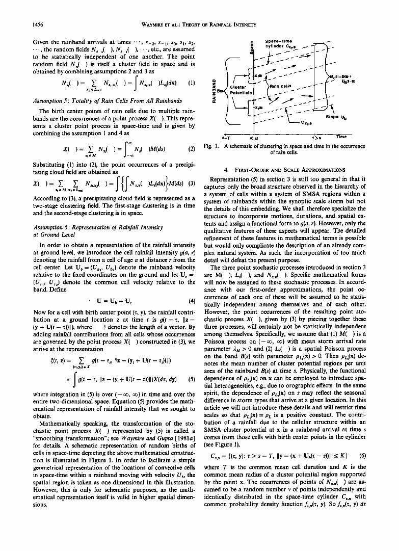
Mathematically speaking, the transformation of the sto- chastic point process X( ) represented by (5) is called a "smoothing transformation"; scc Waymire and Gupta [1981a] for details. A schematic representation of random births of cells in space-time depicting the above mathematical construc- tion is illustrated in Figure 1. In order to facilitate a simple geometrical representation of the locations of convective cells in space-time within a rainband moving with velocity U0, the spatial region is taken as one dimensional in this illustration. However, this is only for schematic purposes, as the math- cmatical representation itself is valid in higher spatial dimen- sions.

Space -time • cylinder Cx,,s

• x,=.•........---"" r• .-. UbCt_s) z

,•_ ter /Rain cells ... z_ • Potentia "'" '" • "-----k. -

Slope U b

I

s-T (O,s) t > s Time

Fig. 1. ^ schematic oœ clustering in space and time in the occurrence oœ rain cc]]$.

4. FIRST-ORDER AND SCALE APPROXIMATIONS

Representation (5) in section 3 is still too general in that it captures only the broad structure observed in the hierarchy of a system of cells within a system of SMSA regions within a system of rainbands within the synoptic scale storm but not the details of this embedding. We shall therefore specialize the structure to incorporate motions, durations, and spatial ex- tents and assign a functional form to g(a, r). However, only the qualitative features of these aspects will appear. The detailed refinement of these features in mathematical terms is possible but would only complicate the description of an already com- plex natural system. As such, the incorporation of too much detail will defeat the present purpose.

The three point stochastic processes introduced in section 3 are M( ), Ls( ), and Ns,x( ). Specific mathematical forms will now be assigned to these stochastic processes. In accord- ance with our first-order approximations, the point oc- currences of each one of these will be assumed to be statis-

tically independent among themselves and of each other. However, the point occurrences of the resulting point sto- chastic process X( ), given by (3) by piecing together these three processes, will certainly not be statistically independent among themselves. Specifically, we assume that (1) M( ) is a Poisson process on (-o o, oo) with mean storm arrival rate parameter ,•st > 0 and (2) Ls( ) is a spatial Poisson process on the band B(s) with parameter pt, s(x)> 0. Then pt, s(x) de- notes the mean number of cluster potential regions per unit area of the rainband B(s) at time s. Physically, the functional dependence of pt`.(x) oe, x can be employed to introduce spa- tial heterogeneities, e.g., due to orographic effects. In the same spirit, the dependence of pt`,(x) on s may reflect the seasonal difference in storm types that arrive at a given location. In this article we will not introduce these details and will restrict time

scales so that pt,•(x) -- Pt, is a positive constant. The contri- bution of a rainfall due to the cellular structure within an

SMSA cluster potential at x in a rainband arrival at time s comes from those cells with birth center points in the cylinder (see Figure 1),

Cs,x = {(r, y): r > s- T, Ily- (x + Ub(Z- s))ll _< K} (6) where T is the common mean cell duration and K is the

common mean radius of a cluster potential region supported by the point x. The occurrences of points of Ns.x( ) are as- sumed to be a random number v of points independently and identically distributed in the space-time cylinder Cs,,, with common probability density function fs,,,(r, y). So fs,,,(r, y) dr

WAYMIRE ET AL.' THEORY OF RAINFALL INTENSITY 1457

TABLE 2. A Summary of Typical Ranges of Various Parameters in the Mathematical Construction

Parameter Description Order of Magnitude

0• -1 2rid 2

io

IUcl

rainband arrival rate

mean density of cluster potentials mean number of cells per cluster cellular birth rate

cell location parameters within a cluster potential region

parameter as a measure of mean cell age spatial extent of cell intensity raincell intensity at cell center at the

time of birth

rainband speed relative to the ground cell speed relative to the band

3.86 x 10- '• bands/min 4 x 10- 3 cluster/km2 4

6.6 x 10 -3 cells/min 5.47 km

40 min

30 km • 1.0 mm/min

1.1 km/min 0 km/min*

*See Zawadzki [1973] for details.

dy represents the probability of an occurrence of a birth center point of a cell within dr dy of (r, y) due to a cluster potential at x within a band arrival at time s.

The main scale approximation which we make is to replace the LMSA region B(s) by the entire two-dimensional plane. This, in conjunction with the homogeneity assumption made earlier (i.e., pt:,(x) - PL) means that the cluster potentials occur independently and uniformly throughout the band with mean density pL. To be physically reasonable, this scale assumption requires that the spatial ground region be small compared to the rainband size B(s).

Finally, we need to specify the functional forms of the prob- ability density fs.,,(r, y) governing the occurrence of birth center points within a cluster potential region and the cellular rainfall intensity function g(a, r). Assume that

f•.,,(r, y) = 0 r < s - T

f•.,,(,, y)=f•{•}(r)f{2}(y- (x + Udr- s)))

where

r>s-T (7)

f•{i}(r) = •e-•{'-% -•r r > s- T (8)

I { x12 x2 2} x2) ER2 f½2)(X) -- 2/1:0.•0.2 exp 2 2'•2 • x = (x•, In (7) the random variable corresponding to the probability density function f•x•(r) and governing the birth of cells within a cluster potential region is assumed to be statistically inde- pendent of the variable corresponding to f•2•(y) governing the location of cells in this region. This assumption is in the spirit of a first-order approximation with regard to statistical depen- dencies that may exist in this mechanism. The parameter in (8) then represents the mean time over which cells are born in a cluster potential region and is of the order 2.5 hours (see Table 1). Another point to observe in (8) is that the domain of f•2•(x) is not restricted to the cluster potential region of radius K as it should be. However, because the possibility of oc- currences will be mostly confined to an ellipse with major and minor axes (say, ax and a2, ax -> •2), it is clear that (ax: + •22) x/2 is a measure of K. In this manner, the finiteness of the cluster potential region is incorporated qualitatively in the specification (8). This greatly simplifies integrations without sacrificing the physical picture. The specific form of given in (8) has been derived by Cho [1978] for certain non- precipitating shallow cloud fields [see Gupta, 1983].

The rainfall intensity from a cell of age a at a radius r from

the cell center is assumed to be of the form

g(a, r) = iogx(a)g2(r)

where

gi(a) = e -ø'" a > 0

qi(a) = 0 a < 0

q2(r) = exp {--r2/2D 2} r >_ 0 (9)

and i o is the rainfall intensity at the cell center at the time of its birth. Equation (9) takes rainfall intensities to occur in a spatially symmetrical manner around the cell center, but this assumption can be easily relaxed to incorporate various other geometrical forms. The parameters a-• > 0 and 2•D 2 > 0 are qualitative measures of cell duration T and its spatial extent, respectively. Table 2 specifies typical orders of magnitudes of various parameters introduced in this section.

5. MEAN RAINFALL INTENSITY

The calculation of the mean rainfall intensity from the rep- resentation (5) is based on a calculation of the first-order product density, px{•}(r, y) dr dy, which can be thought of as representing the probability of a cell occurrence within dr dy of the space-time point (r, y). More precisely, it represents the mean number of the cells born around (r, y) due to X( ) (see, for example, Waymire and Gupta [1981a]). Product densities were first introduced into physics literature (see Ramakrishnan [1950] for example). It should be noted that these are not probability densities in the usual sense. For example, the addi- tion rules for total probability do not apply since the events that cells occur at (rx, y•) or (r2, Y2) are not mutually exclu- sive. Nonetheless, as will be demonstrated here, product den- sities are •* .... • ...... t,,1 ;, the a-al?i• c,f the moment struc- ture of the rainfall field in space and time. The following expo- sition is essentially self-contained, but an elementary famili- arity with the concept of product densities will enable the reader to understand better some of the mathematical oper- ations appearing below.

Since px•(r, y) dr dy represents the mean number of cells born around time r at location y, it follows from (5) that the mean rainfall intensity at time t and location z is given by commuting the expectation operation E[ ] with integration,

E[•(t, z)] = f g(t- r, Iz -(Y + U(t- r)) )px{X)(r, y) dr dy (10)

1458 WAYMIRE ET AL.' THEORY OF RAINFALL INTENSITY

Above, and throughout the remainder of this article, the limits of integration with respect to the time variable will be over (-o•, o•) and with respect to the spatial coordinates over the entire two-dimensional plane unless specified otherwise. In view of (2), px•X•(z, y) decomposes further as

px•X•(z, y) = f pNs•x•(z, y)pst•X•(s) ds (11) where p•vs•x•(z, y) dz dy is the mean number of cell occurrences in dz dy around (z, y) within a cluster potential due to a band arrival at time s and p•t•X•(s) ds is the probability of a band arrival within ds of s.

In view of (1), p•x•(z, y) also decomposes as

p•vs•x•(z, y) = f p•v•.x•(z, y)pLs•x•(X) dx (12) where p•v•.x•x•(z, y) dz dy is the mean number of cells in dz 'dy around (z, y) supported by a cluster potential region at x within a band arrival at time s and p,•s<•(x) dx is the mean number of cluster potentials around x in a band arriving at time s.

Invoking the first-order assumptions introduced in the last section,

In addition,

ElM(ds)] = p•t(i)(s) ds =/l•t ds

E[Ls(dx)] = PLs(1)(X) dx = PL dx

(13)

(14)

pN•,,,<X•(r, y)= (V)fs,,•(r, y) (15)

where (v) is the mean number of cells per cluster and fs.x(r, Y) is given by (7). Substituting (15) and (14) into (12), we obtain

p•v•x•(r, y)= (v) •fs.,,(r, y)pr dx = (V)fs(•)(r) •f(2)(y_ (x + Ub(r- s)))Pt. dx = (v>fs(x)(r)pr (16)

since the integration in (16) is over the entire spatial plane as per the scale approximation introduced earlier.

Now substitute (16) into (11) and use (13) to get

px{t•(r, y) = (v)Pt, f ds = (v)Pt,•M (17) Finally, the substitution of (17) and (9) into (10) gives,

E[•(t, z)] = (v)p•/l•t f g(t- r, z- (y + U(t- r))[[)dr dy = (v)p•/l•tio2nD2o• - • (18)

According to (18), the mean intensity at (t, z) is directly pro- portional to the mean number of cells per cluster potential (v), the mean number of cluster potentials per rainfall band p,•, the mean number of bands per unit time/l•t, and the cell intensity io. The constant D20• - x can be viewed as a shape parameter for the cell intensity in space-time. Calculation of the expressions in (16) and (17) are no less important in the context of physical observables, since the long-term goal of studies such as the present one is to relate such aspects of the rainfall field to the dynamics of precipitation.

6. RAINFALL INTENSITY COVARIANCE

IN SPACE AND TIME

The calculations in this section are similar in spirit to those of section 5 but algebraically are more difficult. Only those steps are presented here which contribute to a conceptual un- derstanding of the mathematical model. The purely technical aspects of the calculations are relegated to three appendices. Throughout this section the second-order product density of any point stochastic process, say X( ), will be denoted by px(2)(rl, Yl; r2, Y2)- The mathematical definition of the second- order product density

E[X(dr•, dyl)X(dr2, dy2) ]

= px{2)(rl, Yl; r2, Y2) dr1 dr2 dyl dy2 (19)

represents the mean number of point occurrences of the pro- cess X( ) simultaneously in small neighborhoods of (rx, Y l) and (r2, Y2). It can also be thought of as the probability of simultaneous point occurrences in small neighborhoods around (rl, Yl) and (r2, Y2) as an aid to understanding product density.

We begin with representation (5) to get

E[•(tl, z,)•(t2, z2)] = J1 -{- J2 (20)

where

•/(t2- '172, IIZ2- (Y2 q- [J(t2- r2)) )

ß px{2•(rl, Yl; r2, Y2) dr• dyl dr2 dy2 (21)

J2 = f a(tl - •, I Zl - (y + U(ta - •)) ) ß a(t2 - r, z2 - (Y + U(t2 - r))l )Px½I)( r, Y) dr dy (22)

The first-order density px{•(r, y) appearing in J2 was calcu- lated in section 5 and is given by (17). The steps required to compute J2 by a direct integration seem to be untenable if attempted directly. However, it is possible to use some basic analytical results from probability theory to arrive at the value of J2 somewhat indirectly. The details are given in Appendix B. For convenience we record the result here as

1 -•ltt J2 =- (V)PL}CMiO 2 • e

ß rid 2exp -•'•{[zxx-z2x-Ul(tl-t2)] 2

q- [2,12 -- 2,22 -- U2(t I -- t2)32}} (23) The evaluation of J1 given by (21) requires that px(:•(rl, Yl;

r2, Y2) be calculated first. Since X( ), given by (2), is a clus- tered point stochastic process it follows that (see, for example, Daley and Vere-Jones [1971, p. 343])

px(2)(rl, Yl; r2, Y2) = f Plvs(2)(rl, Yl; r2, Y2)PM½I)(S) ds .I (1)( r , (2) q- PNst(1)(rl' Yi)PNs2 , 2 Y2)PM (24)

Sl • S2

' (S 1, S2) ds1 ds2

The important formula given in (24) for computing the

WAYMIRE ET AL.' THEORY OF RAINFALL INTENSITY 1459

second-order product densities for a clustered point stochastic process such as X( ) will be used repeatedly in the sequel. Physically, (24) may be understood as reflecting the fact that the occurrences of cells at (rl, yl) and (•2, Y2) may be due to a single rainband at time s or due to two distinct rainbands at s• and s 2. Similarly, the second-order product density for given by (1), may be expressed as

p (2)(T ß ; (2)(T 1 ß N, 1, Yl, T2' Y2) = PNs.x , Yl, T2• Y2)PL,{1)(x) dx

Xl •X2

ß (x•, x:) dx• dx: (2•)

Again in (25) the possibility of either one or two different cluster potentials contributing to the occurrences of cells at (•, y•) and (•2, Y2) is incorporated.

In view of the postulates on the structure of the stochastic processes Ls( ) and Ns,x( ) we have

PLs{2)( xl, X2) = PL 2 (26) and

(2) T . Pss.x ( •, Y•, r2, Y2)= (v(v- 1))fs,x(r•, y•)fs,x('C2, Y2) (27)

where ( ) denotes the expectation E[ ]. Substituting (27) together with (14) and (15) into (25), we obtain

p (2)/.r ß N, •i, Yl 'C2, Y2)= ll + 12 (28)

where

I• = f (v(v- 1))fs.x0:l, Y•)fs,x('C2, Y2)Pœ dx (29) I2= • ; (v)2fs,x•(r•, y•)fs,x2(r2, Y2)pœ2 dx• dx2 (30)

The evaluations of the integrals I• and 12 are given in Appen- dix A, as the calculations do not contribute to a physical understanding of the model. From Appendix A we obtain

I• = {v(v- 1))p•f•{•)(•)f•(•)(•2)•a•a2(2•a•a2)-2

1 _ __ Ubl( r __ r2)] 2 ß exp - 4a•2 [Yxx Y21 •

1 - Ub2(r 1 - r2)] 2} (31) 4a22 [Y•2 -- Y22 12 = (v)2pL2f•{x)(rx)f•{i)(r2) (32)

with yl = (yll, Y12), Y2 = (Y21, Y22), and Ut, = (Ut,,, Ut,2). It follows from (28) that the probability of cell births at times and •:2 at respective locations y• and Y2 due to a rainband whose arrival time s is given by

PNs{2)(•l, Yl; •2, Y2) = / 4zcala2 Pt. exp (zl, yl, •2, Y2)

+ (V)219L2]fs(1)(•l)fs(1)(•2) (33) where

exp 0:l, Yl; •:2, Y2) = exp -- 4a•2 [Y•I -- Y2•

-- Ubl,(•l _ .C2)]2 -- 1 } 4a2 • [Y12 -- Y22 -- Ub2('l•l -- r2)'] 2 (34)

Now, to calculate px(2)(rl, y l' r2, Y2), first substitute (33) and (16) into (24) to get

px{2)('cl, Y•; 'C2, Y2)

:F ] k p,. exp 0:•, Y•' •2, Y2) + (v)2p• 2

ß + f f p•2(v>2fs,"'(r,)fs,{l'(r2)p•'2'(s,, s2) ds, ds2 (35)

Now according to the mean field postulates, M( ) is assumed to be Poissonian; therefore

pM(I)(s) = •M (36)

pM(2)(S1, S2) = •M 2 (37)

Substituting these expressions into (35) and using (8), one ob- tains for r • < r2

px(2}(rl, Yl; T2, Y2)

- p• exp (r•, Yl' r2, Y2) + (V)2pL 2 4•fflff 2

••i•T •••+T . •2 e- 2•Te-•(r• -s•) e-•(•2 -s2• ds 1 ds 2

- 2 k 4•a•a2 p• exp (•, y•; •2, Y2)

+ (v>2p•2]e-•{•-•'• + •2p•2(v>2 (38) A similar calculation as above •ives (38) in the case • • r2- Equation (38) gives an expression for the probability of cell births at times r•, r2 and respective locations y•, Y2 due to the passage of multiple rainbands. Apart from being of interest in its own right, this makes it possible to calculate J• given by (21). These computations are given in Appendix C and are reproduced below only for the case when U = U•'

J• = H• + H 2 + H3 (39) where

2•m•io2•2D4(v) 2p•2 = _

- (40) . [•e-•ltt •1 _ •e-81t•

H3 = (v}2p•m2io2(2•)2D½/•2 (4i)

Let •(a' b2)(x) be defined as

1

,(a; b2•x) - (2•)•/2b e -{•-a•:/2•: (42) Then

H 2 = 2•2•m(v(v-

- U•(t• - t2); 2D 2 + 2a•2Xz2•)

ß ,(z•2 - U2(t• - t2); 2D 2 + 2a22)(z22)

ß _ -

1460 WAYMIRE ET AL.' THEORY OF RAINFALL INTENSITY

Combining (23), (39), and (18), the expression for the covari- ance of the ground level rainfall intensity •(t, z) for the case U = Ub and • •/• is given by

Cov z,)]

= z,)] - z,)]

= 0•e -•1"-'21 exp -•--•/{[z• - z2• - U•(t• - t2)] 2

+ [z•2 -- z22 -- U2(t • -- + 02[]•e -•'lt•-t2l -- 0•e-/qt•-t2l]

+ 03rl(Z• -- U•(t• -- t2); 2D 2 + 2a•2Xz2•)

ß r/(z•2 - U2(t • - t2); 2D 2 + 2a22Xz22)

ß [/•e- •1,, -,:1 _ 0•e- t•l,, -t21] (44)

where

(V)pL2MiO21rD 2 0• = (45)

2/'I.M]•io 2 (V) 2pœ 2/1;2D4 02 = 0•(/•2 _ cz2) (46)

2/r2,•tI•(v(v- 1))Pœio2D 4 0 3 -- 0•(]•2 __ 0•2) (47)

The expression for the variance of •(t, z) can be obtained simply from (44) by substituting t• - t 2 -- t and z• - z2 = z,

Var [•(t, z)] = 0• + (/• - 00{02 + 03(4n) -•

ß [(D 2 + 0.12XD 2 + 0'22)] -1/2} (48)

7. THE ROLE AND LIMITATIONS OF TAYLOR'S HYPOTHESIS IN RAINFALL MODELING

The origin of G. I. Taylor's hypothesis on fluid turbulence dates back to the theoretical and experimental studies on tur- bulence in a wind tunnel by Taylor [1938]. He was attempt- ing to relate spatial correlations with time correlations by assuming that the spatial pattern of turbulent motion, as re- flected in the spatial correlations, is carried past a fixed point by the mean flow speed without undergoing any essential change. The basic requirements for this to hold are uniform mean flow and a low level of turbulence since the agreement between theory and experiment is quite good under such con- ditions.

Taylor's hypothesis was extended to the space-time precipi- tation field in the experimental work of Zawadzki [1973]. However, because it was difficult to separate the components of a storm system, Zawadzki [1973] did not attempt a theoret- ical analysis at the scale of turbulence. Instead he assumed that the instantaneous rainfall intensity ½(t, x) at the ground level is a random field and then undertook an experimental determination of its correlation structure in space and time. He observed that during the development of peak periods of the storm which lasted for the first 110 min, the cells' speeds IU, I relative to the storm speed lull were essentially zero, i.e., the cells and the storm moved with the same speed [Zawadzki, 1973, p. 465, Table 2]. However, during the dissipation period of the storm, in the last 50 min, the cells continued to move with essentially the same speeds, whereas the storm's speed became nearly zero.

Zawadzki [1973, Figure 15] observed that for time lags smaller than 40 min the rainfall intensity covariance satisfied Taylor's hypothesis, which may be expressed as

Cov [•(t•, 0), •(t2, 0)] -- Cov [•(0, 0), •(0, U(t• -- t2))] (49)

t• > t 2 IUI -• IUbl t• -- t 2 < 40 min

In words, (49) says that the autocovariance at some time lag (t• -t2) smaller than 40 min at a fixed but arbitrary spatial point, say 0, is the same as the spatial covariance at some fixed arbitrary time, say zero, between two spatial points separated by the translation distance U(t• - t2).

For time lags (tx- t2) greater than 40 min the auto- covariance on the left-hand side of (49) was found to fall sig- nificantly below the spatial covariance function on the right- hand side of (49) and therefore Taylor's hypothesis did not hold, i.e.,

Cov 0), 0)] <Cov 0), u(t - t,))] (50)

t• > t 2 IUI -lull t• -- t 2 _> 40 min

In order to investigate the extent to which the empirical observations contained in (49) and (50) agree with the theoreti- cal expression for the covariance function derived in the last section, first take U = LI b. Then the rainfall covariance is given by (44). Now, substituting t• = t 2 = 0 and z• = 0, z2 = U(t•- t2) into (44), the spatial covariance at an arbitrary time, say 0, is obtained as

Cov [•(0, 0), •(0, U(t• - t2))]

=0• exp[ - (U•2 + U22Xt•- t2)2.] 4D 2

- 2XD2 -1/2 q- (1• - 00 02 q- 03(4/1: ) •[(O 2 q- 0'• q- 0'22)]

U,Z(t, -- t2) 2 UzZ(t, -- t2)21• ß exp -- 4(D2 + a,2) - •-• •_- •r• ']J (51) Now, substituting z• - z 2 - 0 into (44), the autocovariance for the lag (t• - t2) at an arbitrary spatial location is given by

Cov 0), 0)]

[ 12 --t2)21 = O•e -•1'•-'•1 exp - •-• (U 1 q- U22)(tl q- (fie -ø4tt - t21 __ ote- tqt• - t21)

- 2XD2 -1/2 ß 0 2 q- 03(4/1: ) •[(D 2 + 0'• + 0'22)]

ß exp [ U'2(t• - t2)2 U22(t' - t2)2]} Let us first consider time lags (t•- t2) smaller than the

mean cell life 0•-•, which is of the order of 40 min to 1 hour (see Table 2), i.e.,

(t 1 -- t2) < 0•-1 (53)

It may be recalled from section 4 that//- • denotes the average time span during which cells are born in a cluster potential region. Therefore //-•> 0• -•. Now (53) and the condition /•- • > o•- • imply that

- t9 (54)

Equations (53) and (54) lead to the approximation

(/•e -•("-':) - cze -t•("-':)) • (/• - cz) (55)

WAYMIRE ET AL.: THEORY OF RAINFALL INTENSITY 1461

0.8.

0.6.

(B)

(A) Taylor• hypothesis holds in this range

(B) Tsylork hypothesis does not hold in this range

ß

•.• • Space-time correlation

• i _•a_.tia_.l .;o_.rr•_.lst i2n_ _ I

I,,,,,, IllIt till Wll ' II1"'!" '! I''''1 i,i •!,fllltl,|l,11,11,,111, ,,, i,iii 0 10 20 30 40 50 60 70 80 90 100

Time Lag (min)

Fig. 2. A plot of correlation function for space-time rainfall intensity.

and

e-•("-'2) g 1 (56)

The expression (52) in conjunction with (55) and (56) becomes equal to that in (51) for time lags smaller than •-•, i.e., the rainfall covariance satisfies Taylor's hypothesis,

Cov [•(0, 0), •(0, U(t, - t2))] • Cov [•(t,, 0), •(t 2, 0)] (57) -1

IUI--IUbl t• -- t 2 < •

For time lags larger than a-•, (55) and (56) do not hold, and therefore Taylor's hypothesis does not hold either. For these time lags, (51) and (52) show that

Cov [•(t,, 0), •(t 2, 0)] <Cov [•(0, 0), •(0, U(t, - t2))] (58) -1

IUI- lull t• -- t 2 _> •

Equations (57) and (58) provide an excellent qualitative expla- nation of the empirical results contained in (49) and (50). Figure 2 gives a plot of the correlation function of the space- time rainfall, i.e., of the expression given by (44), (51), and (52), each divided by the variance (48), for the parameter values reported in Table 2. The reader may notice that the plot of (44) in Figure 2, identified as "space-time correlation," is for time points t• and t 2 -- t• + ß and spatial points z• and z2 = z• + U•, where • is the time lag.

It is important to notice that in a statistical model of a stationary and homogeneous random field, such as construct- ed here and by Zawadzki [1973], the choice of time and spa- tial origins do not affect the results. This important feature is central to understanding Zawadzki's computation and results as well as to their explanation by this theory. Specifically, since Zawadzki had only one sample realization of the precipi- tation field at hand, an estimation of the first two moments by statistical sampling required that the following ergodic as- sumptions be invoked [see Zawadzki, 1973, equation (2.2), p. 459],

(59)

and

x)ds dx = 0)] t--• •)

(60)

where B is some spatial region and IBI denotes its area. Equa- tions (59) and (60) can be meaningfully employed in statistical estimation only when the random field is stationary and ho- mogeneous. If not, then one must obtain several realizations of the random field corresponding to each space and time origin of interest and calculate averages with respect to these .realizations for each such origin. This is certainly impossible to do with Zawadzki's observations since he had only one sample realization of the precipitation field. Therefore station- arity and homogeneity are implicit in Zawadzki's calculations, which led to the empirical spectral features displayed in his Figure 15. Consequently, the spectral features observed by him are valid with respect to any space-time origin within his storm and not only with respect to the beginning of the storm. This important feature is corroborated by the present theory as long as the condition IUI - IUol holds; recall that IUI -IUol for the first 110 min in Zawadzki's observations.

However, if the time origin in Zawadzki's computations was set at 110 min after the storm's initiation, when IUcl 4: 0, then according to the present theory the empirical results would have shown that Taylor's hypothesis is not true for any time lag. This follows from the fact that if IUcl 4: 0, then the general expressions for the covariance in (39) is obtained by substitut- ing the expression for H2 given by (C15) instead of (C16) in Appendix C since the latter is only true when IUcl--0, i.e., IUol- IUI. A brief examination of the expression in (C15) shows that space-time terms interact in it and the rainfall covariance does not exhibit Taylor's hypothesis for any time lag. We speculate on the basis of the present results that the slight difference between the spatial and autocorrelation found by Zawadzki [1973, Figure 15] is not due to experimental errors as suggested by him but rather is due to the fact that IUcl is slightly different from zero in the first 110 min and much more so in the last 50 min. It will be very important to investigate from observations on diverse storms the extent to which these spectral features of the theory apply to other storms.

In summary, the present theory as well as Zawadzki's em-

1462 WAYMIRE ET AL..' THEORY OF RAINFALL INTENSITY

pirical findings show that the validity of Taylor's hypothesis holds only under restricted physical conditions, as when cells' speeds relative to the storm are zero, and holds only for time spans smaller than mean cell life rather than for all times. As discussed in section 8, these important physical limitations on the validity of Taylor's hypothesis in rainfall have not been taken into account in other stochastic rainfall models such as

that proposed by Bras and Rodri•!uez-lturbe [1976] and more recently by S. Lovejoy and B. B. Mandelbrot (unpublished manuscript, 1984).

8. SOME FINAL REMARKS

The set of assumptions given in sections 3 and 4 represents the building blocks of a mathematical model of rainfall inten- sity and embodies many observed qualitative features of the precipitation systems. Zawadzki's qualitative results are not part of these assumptions. Rather Zawadzki's results are derived in section 7 as a mathematical consequence of these observed features. In this sense, this theoretical work es- tablishes an important connection between the general fea- tures of storm structures observed and reported by Hobbs and LocateIll [-1978], Hartold and Austin [-1974], and others and the empirical findings of Zawadzki [1973]. Most importantly, it provides theoretical insights into the physical limitations on the validity of Taylor's hypothesis in rainfall fields.

Rainfall modeling is a multifaceted problem with potential for diverse applications to hydrologic and meteorologic sci- ences such as the design of rainfall measurement networks, physical-statistical investigations of components of the hydro- logic cycle, e.g., streamflows, infiltration, evaporation, etc. The objectives in this connection also mandate that rainfall fields be amenable to numerical simulation. That this is indeed feasi-

ble with the mathematical constructs detailed here has already been answered by J. Valdes of Simon Bolivar University, Caracas, Venezuela. These results will be presented elsewhere in the future. The earlier effort on rainfall simulation is by Bras and Rodriguez-lturbe [1976]. However, their work does not properly capture the space-time evolution of rainfall fields because links between space and time are established strictly by invoking the validity of Taylor's hypothesis for all times. As a result, a given initial spatial pattern of rainfall, as speci- fied by a spatial covariance function, only translates with the large-scale storm speed and does not capture the temporal evolution of the storm for time lags larger than the mean cell life. The same major restriction also appears in more recent simulation models of space-time rainfall by S. Lovejoy and B. B. Mandelbrot (unpublished manuscript, 1984). In this latter reference the Taylor transformation is applied to distributions since second-moment correlations are nonexistent. This in

itself goes beyond the experimental results of Zawadzki as a nontrivial extrapolation not known to be empirically support- ed.

Clearly, additional experimental studies need to be carried out on space-time rainfall for diverse storm types, and their empirically observed statistical features need to be docu- mented to guide further theoretical investigations. On the the- oretical side the mathematical framework developed here can be extended to incorporate additional physical features, e.g., differences in velocities, random rainfall intensities and dura- tions of cells, incorporation of inhomogeneities in the rainfall process via introducing spatial variabilities in some of the parameters like p•(x) which may model orographic mecha- nisms, etc. While introducing these types of features does not pose any major problems in numerical simulations of this

model, it certainly would complicate the analytical picture. On the analytical side it would be important to keep the details to a minimum but to seek theoretical explanations of new em- pirical features of rainfall as they become available.

Another important analytical problem area is that of calcu- lating scaling limits of random fields constructed here (see, for example, Burton and Waymire [1984]). Typically, a scaling limit would describe the evolution of the fluctuations in space- time averages of rainfall intensity at suitably chosen scales. In a description of the averages, e.g., via a central limit theorem- type result, many of the details incorporated in the description of the rainfall intensity would not affect the limit behavior because they get "averaged out." In this manner one may hope to get some universality in the descriptions of rainfall fields. However, for such a procedure to work it is imperative that appropriate statistical dependencies be physically understood and incorporated in the mathematical model, as it is the range of dependence which furnishes the scaling parameter and character of the limit, for example, exponential versus power law decay of correlations when these exist. In this respect, the fractal model of Mandelbrot [1982] is being explored by S. Lovejoy and B. B. Mandelbrot (unpublished manuscript, 1984) on the basis of presumed long-range statistical dependence. The extent to which this assumption is consistent with Za- wadzki's [1973] measurements in widespread rain is not clear since in addition to long-range dependence the Lovejoy and Mandelbrot model precludes the existence of correlations. All that one can say on the basis of Zawadzki's data is that (as- suming existence) the correlation decay with distance and time appears to be exponential: dropping to 1/e in distances of 20-30 km in times of roughly 30 min. The justification of the propriety of long-range dependence is often suggested with an appeal to the Hurst phenomenon (S. Lovejoy and B. B. Man- delbrot, unpublished manuscript, 1984). However, the Hurst phenomenon simply does not imply long-range dependence [see Bhattacharya et al., 1983].

At a more basic level it will be important to establish the extent to which the statistical properties of rainfall fields such as the one developed here can be tied with the physics gov- erning the formation and propogation of storm systems. Nee- dless to say, atmospheric processes in general and precipi- tation in particular at the mesoscales seem to be coupled to processes at the larger scales [Leafy et al., 1983]. While we seek to predict and understand precipitation, we are con- strained by a lack of understanding of how small-scale pro- cesses affect those at the larger scales via instabilities and turbulence and vice versa. Some interesting preliminary results which exemplify this direction have recently been obtained by Leary et al. [1983]. It is precisely a search for these connec- tions which mandates a need for theories which couple pre- cipitation dynamics at the larger scales with statistical descrip- tion at smaller scales of interest. A great deal of research needs to be carried out on this problem.

APPENDIX A

In this appendix the integral contributions to the probabil- ity of cell births at times z•, z2 at respective locations y•, y2 due to a rainband arrival at time s will be obtained as re-

quired in (28). The following identity plays a basic role in this calculation:

{-[(w- + - = x/•a exp {-(w - z)e/4•r:} (A1)

WAYMIRE ET AL.: THEORY OF RAINFALL INTENSITY 1463

By completing the square in the exponent on the left-hand side of (A1) the integrand may be viewed as a product of exp {-(w - z)2/4a e) times a nonnormalized normal density in the variable # with mean «(w + z) and variance «ae. Identity (A1) then follows easily.

The following two propositions are essentially consequences of (A1).

Proposition A1

I 1 = (v(v- 1))p•.fs{1)(rl)fs{1)(r2)•rala2(2•rala2) -2

ß exp -- • [Yll -- Y21 -- Uot(*l - *2)] 2 4al 2

4aee [Yle -- Yee -- Uo:(*l - *2)] 2 (A2) where

Yl = (Yll, Yl2) Y2 = (Y21, Y22) U• = (U•,,, U•,:)

Proof: First, substitute (7) into (29) to get

I 1 = (V(V-

ß _ (x + uo(,, - s))]f(2)[y 2 -(x + ub(, 1 - s))] dx Now, substitute (8) into the integral and apply (A1) to each of the iterated integrals with respect to x = (x l, x2) to obtain (A2).

Proposition A2

12 = (V)2pt`2fs(1)(* l)fs(1)(*2) (A3)

Proof: Substitute (7) into (30) to get

12 =

ß ff<2•Eyl- (xl + U,(*l- s))'l dxl f•2•EY2- (x2 + U,(*2- s))] dx2

Now, observe from (8) that these functions in two dimensions, for example, f<2•Ey 1 - (x, + U•(,, - s))] = f<2)Exl - Y, + U•(*l- s))'] may be viewed as a two-dimensional normal

density with mean Y l- U•(*l- s) and a diagonal variance- covariance matrix. Therefore it follows that

f(2)Eyl -- (xl + U•(, 1 - s))] dxl = •f(2)[y 2 --(X 2 q- Ub(* 2 -- S))] dx 2 = 1

APPENDIX B

In this section we shall evaluate the integral J e given by (22).

Proposition B1

J2 = (v)Pt`'•Mio 2 1

{1 •rD 2 exp --•-• [[zll -- z21 -- Ul(tl - t2)] 2

q- [212 -- 222 -- U2(t 1 -- (B1)

Proof: Substitution of (17) into the expression (22) for Je gives

J2 = <v>p,.&,; a(t, - ,, IIz, -(y + U(tl - *)) ) ß •t(t2 -- *, IIz2 -(y q- U(t2 -- 0)ll) d, dy (B2)

Now, substitute (9) into (B2) to get

J2 = (v)Pt,'•MiO 2 • gl(tl -- *)gl(t2 -- *) f ge( IZl -- (Y + U(tl -- *))I)g2( z2 -- (Y + U(te - *))l) dy d,

(B3)

Write the spatial integral coordinatewise and apply the identi- ty (A1) to each set of components in succession, i.e., with zl = (zl•, z•2), U = (U1, U2), and y = (Yl, Ye), to get

J2 = (v)Pt`;cMio 21rD2

1 ß exp --•--•-/ [[(211 -- 221 -- Ul(t 1 -- t2)] 2

q- [212 -- 222 -- U2(t 1 - t2)]2]} f ql(tl -- *)•/1(t2 -- *) d, (B4)

Finally, substituting (9) into (B4) and integrating with respect to ß gives (B 1).

APPENDIX C

The calculations in this appendix are more difficult than any of the precedingß The goal is to evaluate J1 given by (21). Substituting (38) into (21), it can be written as

J1 = H1 + H2 + H3

where

Hl=2--•(v)2p•.2••g(tl--,1, zl -- (yl + U(tl - ,)) ) ß 9(t2- *l, IIz2- (Y2 q- U(t2- *2))ll) e-•l•'-•21 d*l dyl d*2 dY2

2 4r•ala2

IIz, - (yl + u(tl - *x))11)

(c1)

(c4)

The calculations of H1 and H 3 are rather straightforward. It is He that will require special consideration.

First, note that by (18), H 3 is simply 1

2 2

H3 = E[•(tl, zl)]E[•(t2, z2)] '-- (¾> Pt. •.M2iO 2 7 (2•r)2D4 (C5)

(C2)

1464 WAYMIRE ET AL.: THEORY OF RAINFALL INTENSITY

In the case of H1, first use the spatial normalization in (9) to get

• •exp -}-•-/(x 2 + y2) dx dy = 2rid 2 (C6) Substituting (9) into (C2) and first carrying out the spatial integration as given in (C6), H1 reduces to

H 1 = --• (v)2pœ2(27rD2)2io 2

f_2 •_t• gl(tl _ zl)gl(t2 _ z2) e-t•l•-•21 d•:l dz2 Now, carrying out the time integration, H1 is obtained as

2)•M•iO 27r2 D4 ( v ) 2pœ2 H1 = •(//2 _ •2)

(C7)

The calculation of H 2 can be carried out by using the fact that the convolution of independent normal densities is a normal density with new parameters obtained by addition. This fact, which we record more precisely in the next lemma, avoids the inherent complexity in carrying out the integration in H2.

For lemma (C8), let

r!(a; b2)(x) - (2•)•/2b exp - •-• (x - a) 2 (C8) and

ß 2) . = f•o• ' ' q(a• b• ß r/(a 2, b22)(x) r/(al, b•2)(x - y)r/(a 2, b22)(y) dy

Then

r!(a•; b12)* r/(a2; b22)(x)-- r!(al + a2; bl 2 + b22)(x)

We now examine H 2 in the context of lemma (C8). First, substitute (9) and (34) into (C3) to get

H 2 - 2 4•rala 2 PLiø2 f •l(tl -- •l)•l(t2 -- •2)e-•1•-•21

ß g2(llzl -(Y, + U(t, - r,))ll)g2(llz2 -(Y2 + U(t2 - r2))11)

1 __ __ Ubi(Zl •2)] 2 ß exp - 4o.•2 [Yll Y21 1

4o' 2 2 [Y•2 - Y22 - Ub2(*• - *2)] 2} dy11 dy12 dy21 dy22 d*l d'r 2 (C9)

where y• =(y•, Y12); Y2-- (Y2•, Y22), and Ub=(Ub•, Ub2 ). Also recall that z• = (z•, z•2), z2 = (z2•, Z22), and U = U2). Now, observe that integration with respect to Y ll in (C9) can be expressed as a convolutionß Therefore (C9) may be expressed as

iMfl (V(V- 1)) 2 f •(t --*l)g (t2- •2) e-•lrl-r21 H2 - 2 4•ala2 Pcio g I 1 (2•)•/2Dq(zi• - Ul(t• - •1); D2)

* (2n)l/2(•a•)•(-U•,(rl - *2); 2a12)(Y21)

exp - • [z12 - (Y12 + U2(tl - rl))] 2 g,(llz2 -(y2 q- u(t2 - w2))11)

ß exp - 4o'2 • [y12 - y22 - Ub2('rl -- •2)] 2 dy12 dy21 dy22 d•l d•; 2

Now, apply lemma (C8) to get

(ClO)

XMfi (V(V- 1)) PLiO 2 f gl(tl _ •1)g1(t2 _ •2)e_t•l•_•2 I H2- 2 47ro'lo' 2 ß 2nDx/•alr!(z11 - Ul(t• - •1) -- Ub•(* 1 -- Z2); D 2 + 2012)(Y21)

ß exp -- • [z12 -- (Y12 + U2(tl - z1))] 2 g2 ß (11z2 -(y2 + u(t2 - •2))11)

ß exp - 4ff2 • [Y12 - Y22 - U•2(Zl -- z2)] 2 dy12 dy21 dy22 dr1 dz2 (Cll)

Now observe that integration with respect to Y21 in (C11) can again be expressed as a convolutionß This yields

2• (v(v- 1)) P•iø 2 f al(tl - •1)a1(t1 - •1) H2- 2 4nala 2 ' e-•l'•-•212nD•ai(2n)i/2D•(Ui(t2 - •2); D2) ß •(Zll - Ul(ti - Zl)- U•(zl - z2); D2 + 2ff12)(z21)

ß exp -• [z12 -(Y12 + U2(tl - r•))]2

ß exp - • [z22 - (Y22 + U2(t2 - r2))] 2

ß exp -- 4a2 TM [Y•2 -- Y22 -- U•2(• - z2)] 2 ß dy12 dy22 dzi dz 2

Apply the lemma (C8) again in (C12) to get

2•fl (v(v- 1)) 2 f 1(tl rl)ql(t2 z2)e -•1•-•21 H2- 2 4nala 2 P•iø q -- -- ß 4•3/2D2ffi•(zil -- Ul(t • - t2)

+ (U1 - U•t)(zl - z2); 2D2 + 2012•z21)

ß exp - • [z•2 - (Y•2 + U2(t• - •))]2

ß exp -• [g22 --(Y22 + U2(t2 -- z2))] 2

ß exp -- 4ff2 • [Y12 -- Y22 - U•2(zl - z2)] 2 ß dye2 dy22 dZl dr2 (C13)

By symmetry we will get a similar result for the remaining two integrals with respect to the coordinates Y•2 and Y22. There- fore

2mfl (v(v- 1)) PLiø 2 • (4•3/2D2ffl)•(zii _ Ul(t • _ t2 ) H2- 2 4nala 2 + (U1 - U•Zl - •2); 2D2 + 2a12•z21)

ß (4•3/202a2)•(z12 -- U2(t 1 - t2)

(c•2)

WAYMIRE ET AL.: THEORY OF RAINFALL INTENSITY 1465

+ (U2 -- Ut•2X'rt - 'r2); 2D 2 + 20'22Xz22)

ß •/t(tt - 'rt)•/t(t 2 - 'r2)e -•l•-•21 d•:t d'r 2

or

H 2 = 2rt2,•MJ•(V(V -- 1))pt, io2D a'; r/(z11 -- Ul(t I - t2) + (U1 - Ut,•X'r• - •:2); 2D2 + 20'•2Xz2•)

ß r/(zx2 - U2(t • - t2) + (U2 - Ut•2)

ß ('rx - 'r2); 2D 2 + 2ax2Xz22)

ß gl(tl - *l)gl(t2 - 'r2)e -•1•-•21 dzx d'r2 (C15)

Now observe that if U = Ub, then the normal densities ap- pearing in (C15) no longer depend on ,•, *2. This is a critical observation which is discussed in connection with Taylor's hypothesis in section 7. In this case the time integral can be evaluated explicitly, leading to

H 2 = 2•r2,•M(v(v- 1))pt. io2D4rl(Ztt - Ut

ß (tx - t2); 2D 2 + 20'x2Xz2•)

ß r/(zx2 - U2(t • - t2); 2D 2 + 20'22Xz22)

ß ]• -0qt -t21 -•ltt-t2l'] ' (C6)

This completes the calculation of J• = H• + H 2 + H 3.

(C14)

Acknowledgments. This research was supported in part by grants CME-7907793 and CEE-8303864 from the National Science Founda- tion.

REFERENCES

Austin, P.M., and R. A. Houze, Jr., Analysis of the structure of precipitation patterns in New England, J. Appl. Meteorol., 11, 926- 934, 1972.

Bhattacharya, R. N., V. K. Gupta, and E. C. Waymire, The Hurst effect under trends, J. Appl. Probab., 20(3), 649-662, 1983.

Bras, R. L., and I. Rodriguez-Iturbe, Rainfall generation: A non- stationary time-varying multidimensional model, Water Resour. Res., •2(3), 450-456, 1976.

Burton, R., and E. Waymire, Scaling limits for point random fields, J. Multivariate Anal., in press, 1984.

Cho, H. R., Some statistical properties of a homogeneous and station- ary shallow cumulus cloud field, J. Atmos. Sci., 35, 125-138, 1978.

Daley, D. J., and D. Vere-Jones, A Summary of the Theory of Point Processes, edited by P. Lewis, John Wiley, New York, 1971.

Gupta, V. K., Stochastic modeling of rainfall in space and time, paper presented at the 2nd International Symposium on Statistical Clima- tology, World Meteorol. Organ., Lisbon, Portugal, Sept. 1983.

Gupta, V. K., and E. C. Waymire, A stochastic kinematic study of subsynoptic space-time rainfall, Water Resour. Res., 15(3), 637-644, 1979.

Harrold, T. W., The structure and mechanism of widespread precipi- tation, Q. J. R. Meterol. Soc., 99, 232-251, 1973.

Harrold, T. W., and P.M. Austin, The structure of precipitation systems--A review, J. Rech. Atmos., 8(1-2), 41-57, 1974.

Hobbs, P. V., and J. D. Locatelli, Rainbands: Precipitation cores and generating cells in a cyclonic storm, J. Atmos. Sci., 35, 230-241, 1978.

Houze, R. A., Structure of atmospheric precipitation systems: A global survey, Radio Sci., 16(5), 671-689, 1981.

Leary, C. A., D. R. Harragan, and H. R. Cho, Precipitation dynamics as a stochastic process, paper presented at the 2nd International Symposium on Statistical Climatology, World Meteorol. Organ., Lisbon, Portugal, Sept. 1983.

Lopez, R. E., Radar characteristics of the cloud populations of tropi- cal disturbances in the northwest Atlantic, Mon. Weather Rev., 104, 268-283, 1976.

Mandelbrot, B. B., The Fractal Geometry of Nature, W. M. Freeman, San Francisco, Califi, 1982.

Orlanski, I., A rational subdivision of scales for atmospheric pro- cesses, Bull. Am. Meteorol. Soc., 52, 1186-1188, 1975.

Petterssen, S., Weather Analysis and Forecasting, vol. 2, McGraw-Hill, New York, 1956.

Ramakrishnan, A., Stochastic processes relating to particles distrib- uted in a continuous infinity of states, Proc. Cambridge Philos. Soc. 46, 595-602, 1950.

Rodriguez-Iturbe, I., and J. M. Mejia, The design of rainfall networks in time and space, Water Resour. Res., 10(4), 713-728, 1974.

Taylor, G.I., The spectrum of turbulence, Proc. R. Soc., London Ser. A, 164, 476, 1938.

Waymire, E. C., and V. K. Gupta, The mathematical structure of rainfall representations, 2, A review of the theory of point processes, Water Resour. Res., 17(5), 1275-1285, 1981a.

Waymire, E. C., and V. K. Gupta, The mathematical structure of rainfall representations, 3, Some applications of the point process theory to rainfall processes, Water Resour. Res., 17(5), 1287-1294, 1981b.

Zawadzki, I. I., Statistical properties of precipitation patterns, J. Appl. Meteorol., 12, 459-472, 1973.

V. K. Gupta, Department of Civil Engineering, University of Mis- sissippi, University, MS 38677.

I. Rodriguez-Iturbe, Universidad Simon Bolivar, Apartado Postal No. 80.659, Caracas 108, Venezuela.

E. Waymire, Department of Mathematics, Oregon State University, Corvallis, OR 97331.

(Received October 21, 1983; revised May 25, 1984; accepted June 4, 1984.)