A semi-implicit approach for sediment transport models withgravitational effects

J. Garres-Dıaz∗, E.D. Fernandez-Nieto†, G. Narbona-Reina† ‡

April 28, 2021

Abstract

In this work an efficient semi-implicit method, which is based on the theta method, for sedimentbedload transport models with gravitational effects under subcritical regimes is proposed. Severalfamilies of models with gravitational effects are presented and rewritten under a general formulationthat allows us to apply the semi-implicit method. In the numerical tests we focus on the applicationof a generalization of the Ashida-Michiue model, which includes the gradient of both the bedloadand the fluid surface. Analytical steady states solutions (both lake at rest and non vanishingvelocity) are deduced an approximated with the proposed scheme. In all the presented tests, thecomputational efforts are notably reduced thanks to the proposed method without loosing theaccuracy in the results.

Keywords: Sediment bedload transport, Shallow Water Exner model, gravitational effects, semi-implicit scheme.

∗Dpto. Matematicas. Edificio Albert Einstein - Universidad de Cordoba, Spain, (jgarres@uco.es)†Dpto. Matematica Aplicada I, Universidad de Sevilla, Spain (edofer@us.es,gnarbona@us.es)‡All authors were partially supported by the Spanish project RTI2018-096064-B-C22 and FEDER

1

1 Introduction

The sediment transport phenomena is a problem of interest in the environmental field. Besides thetypical application in the morphology of a river, the sphere of action of the sedimentation processis wide and it has a deep impact on its environment. Due to the flow of the river some particlesare swept along the current. This material is taken mainly from the riversides and also from thebottom, being deposited downstream when the flow becomes weaker, either again on the riversidesor in its mouth. This effect change the morphology of the river environment sometimes affectingto crops or to natural protected areas but also to fluvial navigation and coastal zones with theconsequent impact in the economy and environmental aspects. It is also important the effect of thesediment transport process in the building of hydraulic structures like dams or bridges. Either thelong-term erosion process or for example in torrential rain events or during the thaw, some of thesediment of the bottom can be dragged and may affect to the stability of these structures. Normallymost of these important phenomena are long-term processes so there is a special interest on thedevelopment of efficient predictive techniques in order to prevent hazards or to better manage thesurroundings.

Sediment transport occurs mainly through two phenomena: bedload and suspended load. Bed-load entails the transport of sediment particles rolling or sliding on the bed and jumping into theflow and then resting on the bed again. Particles transported by suspension are supported by thesurrounding fluid during a significant part of the current and may also be deposited. In this paperwe focus on bedload sediment transport including gravitational effects that is an essential but nottrivial task to take into account in the mathematical modeling.

When the bedload phenomena is under study, we must consider both, the hydrodynamical compo-nent and the morphodynamical one that are coupled. The Saint Venant Exner system is commonlyused to describe the bedload sediment transport and it is a system composed on the well knownSaint Venant (or Shallow Water) system for the hydrodynamics and a continuity equation to up-date the morphodynamical part. This continuity equation is called Exner equation [16], and itis defined in terms of the solid transport discharge that has to be prescribed. In the literatureseveral models have been defined empirically to give this closure [30, 1, 17, 24, 37, 32]. Even ifthese models are largely used they provide some inconvenient properties for the system as the lackof a dissipative energy or the loss of the mass conservation, other important limitation being thevalidation range for just nearly horizontal sediment beds. An alternative to these empirical modelshas been presented in [18] where a complete Saint Venant Exner type model is derived from theNavier-Stokes equations, this model encompassing the former disadvantages.

In classical models, the solid transport discharge is defined in terms of the shear stress and thecritical shear stress, or its normalized form called Shields parameter. Bedload models predict thatthere is no transport of sediment particles whenever the shear stress is smaller than the criticalshear stress, see for instance [16, 30, 1, 17, 24, 37, 32].The Shields parameter is defined as the ratio between the agitating and stabilizing forces on adeposited sediment particle. Lysne [29] showed experimentally for inclined sediment beds that thegravity is an important contributing action as agitating force, see also [20]. Nevertheless classicalformulas consider that the shear stress is the unique agitating force. Therefore, gravitational forcesplay an essential role into the sediment transport, so they must be considered for the definition ofan appropriate solid discharge for applications in general sloping beds.Several forms to include gravitational effects in the solid transport discharge are found in the lit-erature. The simplest one is to include a second order derivative in the Exner equation, which isneglected when the slope of the bed is smaller than the tangent of the repose angle of the material(see Tassi et al. [36]). Nevertheless, the form in which gravitational effects are usually included is

2

by modifying either the definition of the shear stress or the critical shear stress. Although thesetwo kind of modifications might coincide in some particular cases for 1D horizontal domains, theyare not equal in general.Here we consider the inclusion of the gravitational effect in the solid transport discharge, which isdefined in terms of the effective shear stress (see e.g. Fowler et al. [19]). This is discussed in detailby Fernandez-Nieto et al. [18] showing that the solid discharge naturally incorporates gravitationaleffects, which are included in the effective shear stress. Let us also mention that the inclusion ofgravitational effects in the effective shear stress is analogous for scalar or vector systems, that is,1D or 2D horizontal domains. Nevertheless, when the modification of the critical shear stress isconsidered, the inclusion of gravitational effects for 2D domains is not an easy extension of the 1Dcase. See Kovacs and Parker [28], Seminara et al. [35] and Parker et al. [33] among others.

From the numerical point of view, bedload transport models have been usually discretized bymeans of explicit schemes in collocated and staggered meshes (see [6, 7, 31, 3, 25, 18] among manyothers). These problems are characterized by two different time scales: a small characteristic timefor the hydrodynamical counterpart and a large characteristic time for the morphodynamical con-tribution. It makes the computational cost to be very high when explicit discretizations are used,even for simple models (e.g. Grass formula) without gravitational effects. In Bilanceri et al. [4] acomparison of explicit and implicit methods for bedload transport (without gravitational forces)is made, as function of the low/medium/high sediment-fluid interaction. They claim that the fullyimplicit scheme is too much expensive, and a linearization of the method based on the automaticdifferentiation software Tapenade [26] is made to solve the Grass model, showing that the compu-tational cost is decreased, specially in the low interaction case.Just a few works are devoted to numerical approximation of bedload models with gravitationaleffects. In these models, the difficulty from a numerical point of view is the presence of a non-linear elliptic counterpart in the Exner equation. As a consequence, its explicit discretization iscomputationally expensive. Tassi et al. [36] used a Discontinuous Galerkin method to approximatea Grass model with a diffusion term depending on the free surface gradient. Later, Morales deLuna et al. [31] used a duality method based on the Bermumez-Moreno algorithm to solve themorphodynamical component of a Meyer-Peter & Muller model with gravitational effects, whichis computationally more expensive.Therefore, semi-implicit schemes are an interesting and promising alternative in the frameworkof bedload transport models. The method considered here is the one introduced by Casulli andco-worker for hydrostatic [11, 10, 8, 13] and non-hydrostatic [12, 14, 9] free surface flows in z-coordinates and isopycnal cooordinates. In Bonaventura et al. [5] and Garres-Dıaz and Bonaven-tura [23] this method was adapted to vertical multilayer discretization, showing its efficiency whenit is applied to bedload transport with the simple Grass formula, and also for variable densityflows.Such a semi-implicit approach was used in Garegnani et al. [21, 22], where an analysis of thecoupled and decoupled approach of the Exner equation is made, introducing also a semi-implicitmethod ([34]) for the system with movable bed, although they did not consider gravitational effects.

The main contribution of this work is a low-computational cost semi-implicit scheme for sedi-ment transport problems solved through the Saint Venant Exner system introduced in [18] takinginto consideration also gravitational effects, in long-time scale, i.e., slow processes. It is based ona reformulation of the solid transport discharge by rewriting the sign function. Furthermore, theproposed method could be easily adapted to a wide range of families of bedload models withgravitational effects, which is also described in this work. Thus, to our knowledge, this is the firstefficient numerical scheme for general bedload models with gravitational effects.Section 2 is devoted to present the model we use, as well as the reformulation of the solid transportdischarge that we propose to apply the semi-implicit scheme to a wide family of models with grav-

3

itational effects. In Section 3 the semi-implicit method is detailed, and the numerical experimentsare in Section 4. Finally, we present some conclusions in Section 5.

2 Saint Venant Exner system with gravitational effects

In this section we present the initial system for the hydrodynamical and morphodynamical coun-terparts. The solid transport discharge including gravitational effects is defined in Subsection 2.2.Once the chosen model is exposed, the reformulation of the solid transport discharge is proposedin Subsection 2.3, where we also analyze the steady solutions of the proposed model. Finally, weshow in Subsection 2.4 how this reformulation could be easily adapted to a wide range of families ofbedload models, depending on both the definition of the solid transport discharge and the effectiveshear stress.

2.1 Initial system

The base system is the well-known Saint Venant Exner system, which is obtained from the couplingof the Saint Venant system (hydrodynamical component) and the Exner equation (morphodynam-ical component). This model is deduced from the non-dimensional Navier-Stokes equations forthe hydrodynamical part together with the Reynolds equation for the evolution of the granularlayer, a detailed derivation and analysis of this model can be seen in Fernandez-Nieto et al. [18].Considering a 1D incompressible fluid with constant density ρ ∈ R, the system reads

∂th+ ∂xq = 0,

∂tq + ∂x(q2/h

)+ gh∂x (h+ b) = −F ,

∂tb+ ∂xQb = 0,

(1)

where (x, t) are the space and time variables, h(x, t) and u(x, t) the height and averaged horizontalvelocity of the fluid, and q = hu is the discharge. The gravity acceleration is denoted by g and Fis a friction term between the fluid and the sediment layer b(x) which will be defined later. Thissediment is transported according to the solid transport discharge Qb that is defined by the chosenmodel for the bedload transport.

Figure 1: Computational domain and notation.

In the deduction presented in [18] the thickness of the sediment layer (denoted by b here andh2 in [18]) is subdivided in a lower static layer and a small upper movable layer whose height is

4

hm (see Figure 1). Simplified models are also presented there, which is the framework consideredin this work. Assuming a quasi-uniform regime, the erosion rate equals the deposition rate and hmca be estimated in terms of the the rest of unknowns of the problem.

Let us denote the shear stress by τ , which can be written, in the framework of depth-averagedmodels, as τ = ρghS with S a friction term, whose more common definitions are through theManning (S = n2u |u|h−4/3, n the Manning coefficient) or Darcy-Weisbach (S = ξu |u| /8gh, ξ theDarcy-Weisbach coefficient) laws, depending on the averaged velocity u. Then, we can write

τ

ρ= C |u|u, with

C = gn2h−1/3 (Manning law),

C = ξ/8 (Darcy-Weisbach law).(2)

An empirical formula is used to define the solid transport discharge as a closure to the system,for instance Grass [24], Meyer-Peter & Muller [30], Ashida & Michiue [1], among many others. Forinstance, when the classical Ashida & Michiue’s model is chosen, it is written in nondimensionalform as

QbQ

= sgn(τ)17

1− ϕ(θ − θc)+

(√θ −

√θc

), (3)

where ϕ is the porosity of the sediment bed, sgn(·) is the sign function, (·)+ the positive part,

and Q = ds√g (1/r − 1) ds the characteristic discharge that is defined in terms of the gravity, the

density ratio r = ρ/ρs, with ρs and ds the density and the diameter of the sediment particles.Finally, θ is the so-called Shields parameter, defined by

θ =|τ |d2

s

g (ρs − ρ) d3s

,

with θc the critical Shield stress.A general formulation that includes a great number of classical models for the bedload solid

transport discharge without gravitational effects may be written under the following compact form(see [18])

QbQ

= sgn(τ)α1

1− ϕθβ1 (θ − α2θc)

β2+

(√θ − α3

√θc

)β3

, (4)

with αi, βi i=1,2,3 positive constants.Some important drawbacks of these classical models for the bedload transport are: (i) they

do not take into account gravitational effects, since they are derived using as hypothesis thatthe sediment free surface is almost constant ∂xb ≈ 0; (ii) they do not satisfy a dissipative energybalance; (iii) the mass of sediment may be not conserved. In this work we study gravitational effectsin models satisfying a dissipative energy balance. We consider the case of quasi-uniform regimes,where the movable thickness of sediment is set in terms of the velocity of the fluid. In these casesthe mass conservation will not be guaranteed but it can be easily solved as detailed in the followingsubsection. Models including gravitational effects are presented in following subsections.

2.2 Solid transport discharge with gravitational effects

In this subsection, following [18], we present the generalization of the Ashida-Michiue and Meyer-Peter & Muller models under the assumption of a quasi-uniform regime. The general definition ofthe solid transport discharge is

Qb = hmvb√

(1/r − 1)gds,

5

where hm is the thickness of the movable bed and vb the averaged sediment velocity. This velocityis defined in terms of the effective shear stress (τeff) as follows

vb = sgn(τeff)(√θeff −

√θc)+, (5)

with

θeff =|τeff|/ρ

(1/r − 1)gds,

where τeff must be properly defined. Here, following [18], we consider (see discussion in Subsection2.4)

τeff

ρ=

τ

ρ− ϑgds

r∂x (rh+ b) , with ϑ =

θctan δ

, (6)

being δ the angle of repose of the material. Frequent values for these constants are θc = 0.047and ϑ = 0.1, that is θc/ϑ ≈ tan 25◦ (see Fredsœ in [20]). Other possibilities are used in [15] andreferences therein.

We can establish the relation between θ and θeff by computing τ from the previous equation,obtaining

θeff =

∣∣∣∣sgn(u)θ − ϑ

1− r∂x (rh+ b)

∣∣∣∣ ,where sgn(u) is identified as the sgn(τ) and we used the definition of τ in (2).

In order to set the definition of hm we will consider the case of a quasi-uniform regime, wherehm is defined by a closed formula as a function of the erosion and deposition rates (see [18] andreferences therein for further details). A possibility is to define

hm =Keds

Kd (1− ϕ)(θeff − θc)+ , (7)

with Ke,Kd constant parameters related to the erosion and deposition effects respectively. Let usremark that Fernandez-Luque and Van Beek [17] observed in the experiments this linear relationbetween the thickness of the movable bed and the shear stress. Most of classical formulas considerthis relation to obtain the solid transport discharge. This linear relation was also observed inBagnold [2] by investigating the momentum transference because of the sediment particles andfixed bed interaction (see also [15]). Notice that the fact of using a closure formula for hm as abovemay be the mass conservation fail, see [31]. Nevertheless, this problem is solved by defining hm asthe minimum between the definition (7) and the thickness of the erodible sediment layer. In thiswork we consider that this layer is large enough, since a fixed bedrock has not been taking intoaccount.By using the definition of hm (7) we obtain the following formula of the solid transport discharge

QbQ

= sgn (τeff)Ke

Kd (1− ϕ)(θeff − θc)+ (

√θeff −

√θc)+ where Q = ds

√(1/r − 1)gds. (8)

Note that this is a generalized Ashida & Michiue’s model (3), where the ratio between erosion anddeposition effects is set to Ke/Kd = 17.

Another possibility is to define hm as follows (see [35])

hm =Kds1− ϕ

√(θeff − θc)+(

√θeff +

√θc). (9)

6

In this case we obtain that the solid transport discharge is

QbQ

= sgn (τeff)K

(1− ϕ)(θeff − θc)

3/2+ . (10)

Note that in this case we obtain a generalized Meyer-Peter & Muller model, where the constantparameter is set to K = 8.

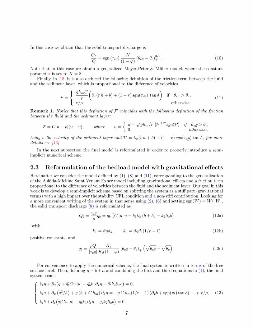
Finally, in [18] it is also deduced the following definition of the friction term between the fluidand the sediment layer, which is proportional to the difference of velocities

F =

ghmC

r

(∂x(r h+ b) + (1− r) sgn(τeff) tan δ

)if θeff > θc,

τ/ρ otherwise.(11)

Remark 1. Notice that this definition of F coincides with the following definition of the frictionbetween the fluid and the sediment layer:

F = C|u− v|(u− v), where v =

{u−

√ghm/r |P|1/2sgn(P) if θeff > θc,

0 otherwise,

being v the velocity of the sediment layer and P = ∂x(r h + b) + (1 − r) sgn(τeff) tan δ, for moredetails see [18].

In the next subsection the final model is reformulated in order to properly introduce a semi-implicit numerical scheme.

2.3 Reformulation of the bedload model with gravitational effects

Hereinafter we consider the model defined by (1), (8) and (11), corresponding to the generalizationof the Ashida-Michiue Saint Venant Exner model including gravitational effects and a friction termproportional to the difference of velocities between the fluid and the sediment layer. Our goal in thiswork is to develop a semi-implicit scheme based on splitting the system as a stiff part (gravitationalterms) with a high impact over the stability CFL condition and a non-stiff contribution. Looking fora more convenient writing of the system in that sense using (2), (6) and setting sgn(W ) = W/ |W |,the solid transport discharge (8) is reformulated as

Qb =τeff

ρqb = qb

(C |u|u− k1∂x (b+ h)− k2∂xb

)(12a)

withk1 = ϑgds, k2 = ϑgds(1/r − 1) (12b)

positive constants, and

qb =ρQ

|τeff|Ke

Kd (1− ϕ)(θeff − θc)+

(√θeff −

√θc

). (12c)

For convenience to apply the numerical scheme, the final system is written in terms of the freesurface level. Then, defining η = b+ h and combining the first and third equations in (1), the finalsystem reads

∂tη + ∂x(q + qbCu |u| − qbk1∂xη − qbk2∂xb

)= 0,

∂tq + ∂x(q2/h

)+ g (h+ C hm) ∂xη = −g C hm(1/r − 1) (∂xb+ sgn(vb) tan δ) − χ τ/ρ,

∂tb+ ∂x(qbCu |u| − qbk1∂xη − qbk2∂xb

)= 0,

(13)

7

where we identified sgn(vb) as the sgn(τeff) and χ =

{1 θc ≥ θeff

0 otherwise.

Regarding the stationary solutions of system (13), it is difficult to obtain an explicit expression ingeneral. However, it is interesting to firstly analyze the simple case concerning lake at rest solutionthat is a steady solution for the Saint Venant system. That is, those ones verifying

b+ h = η0 constant, q = 0. (14)

It is easy to check that they are also steady solutions of previous system if gravitational effects arenot considered (k1 = k2 = 0), since we recover τ = 0 and therefore θ = 0 and Qb = 0. That meansthat solutions given by (14) are steady solutions independently of the sediment layer profile b(x).Obviously, this is a limitation of classical models and non-physical solution will be kept.

On the contrary, this is not the case for the proposed model with gravitational effects. Actually,we have the following result.

Proposition 1. Let η0 constant be the free surface level of a fluid at rest (u = 0), with b(x) thesediment layer and δ the angle of repose of the sediment. Then

(η0, 0, b(x)) is a steady solution if and only if |∂xb| ≤ tan δ.

That is, a lake at rest solution is steady if and only if the sediment layer has a slope lower thanthe slope given by the angle of repose of the sediment.

Proof. Let us start proving that the condition |∂xb| ≤ tan δ is equivalent to θeff ≤ θc under thehypothesis ∂xη = 0, u = 0. In this case

θeff =k2 |∂xb|

g (1/r − 1) ds=ϑgds(1/r − 1)

g (1/r − 1) ds|∂xb| =

θctan δ

|∂xb| ≤ θc,

and this inequality holds if and only if |∂xb| ≤ tan δ.Using the condition θeff ≤ θc, it is easy to check that Qb = hm = 0 (see (7) and (8)), and

therefore ∂tη = ∂tq = ∂tb = 0, i.e, (η0, 0, b(x)) is a steady solution.Assuming now that (η0, 0, b(x)) is a steady solution, we obtain

∂x (k2qb∂xb) = 0 and hm (∂xb+ sgn(vb) tan δ) = 0.

From the first condition, either ∂xb = 0 and therefore τeff = 0 = θeff ≤ θc and also hm = 0, orqb = 0 and therefore (θeff − θc)+ = 0, which ends the proof.

Let us now study steady solutions in the general case, neglecting the friction term χτ/ρ in themomentum equation in (13).

Theorem 1. Let (η(x), q0, b(x)) be the values of the free surface, discharge and sediment layersatisfying that Qb = 0, with q0 constant. Then, it is a steady solution of system (13) if and only ifit satisfies

−sgn (τeff) β ∂xb ≤ tan δ

(1 −

sgn (τeff)C |q0| q0

gdsθc (1/r − 1)

1

(η − b)2

), ∂xη = α∂xb, (15)

with

α =−q2

0

g (η − b)3 − q20

and β = 1 +α

(1/r − 1).

8

Proof. Let us start by noticing that the steady solutions of system (13) with no sediment transportare given by

∂xq = 0, ∂x

(u2

2+ gη

)= 0, Qb = 0. (16)

The first condition implies that q(x) = q0 constant. From the second condition in (16), and writingu as q0/(η − b), we deduce that

∂xη = α∂xb, with α =−q2

0

g (η − b)3 − q20

.

Furthermore, since Qb = 0, the only possibility is that θeff ≤ θc holds, which leads to the inequality∣∣∣∣ tan δC |u|ugdsθc(1/r − 1)

− β∂xb∣∣∣∣ ≤ tan δ, where β = 1 +

α

(1/r − 1). (17)

Now, we can solve the inequality for the unknown ∂xb, taking into account that the sign of the lefthand side coincides with sgn (τeff), obtaining inequality (15), which ends the proof.

Notice that the Proposition 1 is a particular case of the Theorem 1 where q0 = 0, obtainingα = 0 and β = 1 in (17) and η(x) = η0 constant.

When the limit case is considered in (15), i.e. when the equality holds, the explicit expressionsof η and b are the solutions of the resulting nonlinear ODE system. Note that η, b in (15) canbe also found by solving just the initial value problem for the sediment, and updating the freesurface value at each step using conservation of the energy (middle condition in (16)), that isη = b + h where h is the greater root (for subcritical solutions) of the third-order degree polyno-mial 2gh3 + 2(gb−K0)h2 + q2

0 = 0, where K0 = u20/2 + gη0.

In the results presented in this subsection we have focused on the generalized Ashida-Michiuemodel for the sake of simplicity. However, many other Saint Venant Exner models including gravi-tational effects could be written in the same form as (12)-(13), for instance the generalized Meyer-Peter & Muller model defined by (10) for K = 8. In the next subsection other possible general-izations to include gravitational effects are discussed, which can be easily written under the form(12)-(13). Consequently, the same numerical technique that is proposed in Section 3 can be appliedfor this family of models.

2.4 A general formulation of bedload sediment transport modelswith gravitational effects

In this section we briefly present several approaches to include gravitational effects in classicalmodels, and the relations between them. As we commented before, it is suitable for the develop-ment of the semi-implicit method presented in Section 3 if the model is written under the form(12). Thus, all the discussed models below will be expressed in the same way.

In classical models, with the purpose of including gravitational effects, we shall replace τ withτeff and θ with θeff in the solid transport discharge Qb. For example, when considering the familyof classical models defined by the solid transport discharge (4), the corresponding models withgravitational effects are defined by

QbQ

= sgn(τeff)α1

1− ϕθβ1

eff (θeff − α2θc)β2+

(√θeff − α3

√θc

)β3

,

9

being α1, α2, α3, β1, β2 and β3 non-negative constants depending on each model.

In addition, note that the effective shear stress must be defined to write previous models un-der the form (12). Actually, a different family of bedload models is obtained for each definition ofτeff proposed in the literature.In the next lines we present some relevant definitions of τeff in order to show the differences andthe similarities, but also to give a justification of our choice given in (6).

Let us begin with the effective shear stress introduced in Fowler et al. [19] that we denote byτFeff and which is given by

τFeff

ρ=

τ

ρ− λ g ds(1/r − 1)∂xb, (18)

where τ is a quadratic law defined as in (2) and λ = 1. Later, Morales de Luna et al. [31] proposedto define λ = ϑ, where ϑ is defined in (6), with the aim of recovering lake at rest steady solutionsassociated to the repose angle of the sediment. Whatever the value of λ, we find a family of modelsthat can be reformulated defining Qb as in (12a), and qb, k1, k2 as follows

qb =ρQ∣∣τFeff

∣∣ α1

1− ϕ(θFeff)β1

(θFeff − α2θc

)β2

+

(√θFeff − α3

√θc

)β3

, (19)

with

θFeff =|τFeff|/ρ

(1/r − 1)gds, k1 = 0 and k2 = λ g ds(1/r − 1).

Note that the definition of k2 is the same that in previous cases (12b), but k1 is neglected. Thismeans that the free surface gradient has no influence on the solid transport discharge when τFeff

is considered. Equivalently, τeff in (6) matches with τFeff if the free surface of the fluid is constant,∂x(b+ h) = 0.

Let us now go deeper in the definition of τeff to understand the expression (6) that we use inthis work. In Fenandez-Nieto et al. [18] the Navier-Stokes system is asymptotically analized todeduce a Saint Venant Exner system, leading to propose several models including gravitationaleffects and satisfying a dissipative energy balance. These gravitational effects are included throughthe considered effective shear stress. The law considered for the drag force between the fluid andgranular layers determines both the model and the effective shear stress. In particular, two expres-sions for the effective shear stress are deduced corresponding to a linear or quadratic friction law,

denoted by τLeff or τQeff respectively, that we present next.In the linear friction case, it is defined by

τLeff

ρ=ϑdshm

τL

ρ− ϑgds

r∂x (rh+ b) , with

τL

ρ=Chmu

√g(1/r − 1)dsϑds

, (20)

or equivalently,τLeff

ρ= Cu

√g(1/r − 1)ds −

ϑgdsr

∂x (rh+ b) . (21)

Now the family of models is given by

Qb =τLeff

ρqb = qb

(Cu√g(1/r − 1)ds − k1∂x (b+ h)− k2∂xb

), (22)

10

where

qb =ρQ∣∣τLeff

∣∣ α1

1− ϕ(θLeff)β1

(θLeff − α2θc

)β2

+

(√θLeff − α3

√θc

)β3

,

and with k1 and k2 as in (12b) for θLeff =|τLeff|/ρ

(1/r−1)gds.

In the quadratic friction case, the effective shear stress is (see [18])

τQeff

ρ= gds(1/r − 1)|Φ|Φ, (23)

where

Φ = sgn(u)

√|τQ|/ρ√

(1/r − 1)gds−

√∣∣∣∣ ϑ

1− r∂x (rh+ b)

∣∣∣∣sgn(∂x (rh+ b)),

with τQ defined in terms of τ (2) as

τQ =hmϑds

τ. (24)

The effective shear stress τQeff (23) gives other family of bedload models, where

sgn(τQeff) = sgn(Φ) and θQeff = |Φ|2,

which can be reformulated under a similar expression to (12a), concretely we obtain

Qb = qb

(u

√ϑdshm

C − k1∂x (b+ h)− k2∂xb), (25a)

with

qb =Q∣∣∣∣u√ϑds

hmC − k1∂x (b+ h)− k2∂xb

∣∣∣∣α1

1− ϕ(θQeff)β1

(θQeff − α2θc

)β2

+

(√θQeff − α3

√θc

)β3

(25b)

and

k1 =

√ϑgdsr√

|∂x(rh+ b)|, k2 =

√ϑgdsr√

|∂x(rh+ b)|(1/r − 1) . (25c)

Note that this model is much more complicate that any of the models defined by (19) or (22).Firstly, because the values k1, k2 are no more constant. Secondly, note that hm can be defined by

(7) or (9), in terms of(θQeff − θc

)+

, and as a consequence θQeff is implicitly defined.

Let us now make a comparison of the three definitions (18), (20) and (23) given for the effec-tive shear stress. When the effective shear stress of the linear model (21) is compared with thedefinition (18) given by Fowler [19], two differences are observed. Firstly, the first term in thedefinition changes, it is quadratic in the velocity for the Fowler’s model and linear in (21), whichis consistent with the hypothesis of a linear drag force between fluid and sediment layer. Secondly,the gravitational terms are different, although they are equal when the free surface is constant andλ = ϑ. It can be easily seen by writing

ϑgdsr

∂x (rh+ b) = ϑgds(1/r − 1)∂xb+ ϑgds∂x (b+ h) .

11

Therefore, the definition of the gravitational effects introduced in [18] is more general, since ittakes into account the weight of the upper fluid and the coupled effect of the variations of the freesurface and sediment.Furthermore, when looking at the effective shear stress deduced for the quadratic model (23) we donot find the same definition than in the Fowler’s model, even if they both correspond to a quadraticfriction law. Moreover the gravitational terms are also different, being much more complex in thequadratic model.

The effective shear stress (6) used in this work may be interpreted as a linearized version ofthe quadratic effective shear stress, corresponding to the definition τLeff (20) when the friction term

τL is replaced by τQ defined in (24), thus obtaining our definition

τeff

ρ=

τ

ρ− ϑgds

r∂x (rh+ b) .

As commented above, this model can be also seen as an enhanced Fowler’s model where thegravitational effects take into account the free surface gradient.Finally, the corresponding family of models for the proposed τeff defined in (6) can be reformulatedeasily keeping Qb as in (12a), that is,

Qb =τeff

ρqb = qb

(C |u|u− k1∂x (b+ h)− k2∂xb

),

but where qb in (12c) is replaced with

qb =ρQ

|τeff|α1

1− ϕθβ1

eff (θeff − α2θc)β2+

(√θeff − α3

√θc

)β3

,

k1 and k2 taken the same values introduced in (12b).

3 Semi-implicit approach

We are interested in this work on the large-time scale, i.e., very slow processes where the charac-teristic time associated to the sediment is very large, and usually the fluid-sediment interaction isweak. This is the case for example of the movement of a dune in a river or a lake. In these situationsit is common to have subcritical regimes. Furthermore, note that second order space derivativesof the free surface and the sediment layer appear in system (13). Then, when discretizing it usingan explicit scheme it leads to a very restrictive stability condition (CFL) and therefore to a hugecomputational cost because of the small time-steps.In this section, we develop an efficient semi-implicit numerical scheme to relax the CFL conditionby removing the gravitational contributions, which can be applied to any model with gravitationaleffect written under formulation (12) −or (25)− and (13). The spatial and time discretizations aredescribed through the finite volume method.

Let us start with the spatial discretization, where we consider a uniform mesh step ∆x with-out loss of generality. Then, we subdivide the computational domain into control volumes denotedby Vi =

(xi−1/2, xi+1/2

)with center xi =

(xi−1/2 + xi+1/2

)/2, for i ∈ I, with # (I) = M . We con-

sider a staggered mesh, that is, the discrete free surface and sediment variables (ηi, bi) are definedat the center of the control volumes (xi), whereas the discrete discharge values (qi+1/2) are at theinterfaces (xi+1/2). This C-grid staggering has the advantage that the linear system resulting fromthe semi-implicit time discretization is more compact.

12

We propose to discretize system (12), (13) using the semi-implicit scheme introduced in [11,10, 8] based on the theta method. This strategy allows us to remove the celerity contribution tothe CFL condition. Thus, defining hi = ηi− bi, ui = (qi−1/2 + qi+1/2)/hi and the Courant numbers

Cvel =∆t

∆xmaxi∈I|ui| , Ccel =

∆t

∆xmaxi∈I

(|ui|+

√ghi

),

with ∆t the time step, the explicit method has a stability restriction that can be approximatedby Ccel < 1, whereas the semi-implicit method relaxes this condition to Cvel < 1. Therefore,in subcritical regime (|u| /

√gh � 1) this approach allows us to give larger time steps since the

restrictive contribution is the gravitational one.The theta method (hereinafter Θ-method) reads

wn+1 = wn + ∆t Θf(tn+1, wn+1

)+ ∆t (1−Θ) f (tn, wn) ,

for an arbitrary ODE system w′ = f(t, w), being Θ ∈ [0, 1] the implicitness parameter. Note thatin the limit cases Θ = 0 and Θ = 1, the explicit and implicit Euler methods are recovered. Asexpected, this method is more diffusive for large values of Θ. In practice, we choose Θ slightlylarger than 1/2, since this method is unconditionally stable for Θ ∈ [1/2, 1].

Since the goal of this work is not to propose high order semi-implicit scheme, we perform adiscretization based on the theta method, which is first order accurate (second order if Θ = 1/2,Crank-Nicolson method). This procedure can be adapted to more accurate time discretizations ifneeded via an IMEX-ARK (Implicit Explicit Additive Runge Kutta) methods (see [27]), followingthe description made in [5, 23].

In the following we describe how the system (13) is discretized. The key point is considering allthe convective terms in a explicit way, while terms involving the derivative of the free surface (∂xη)and the sediment layer (∂xb) are discretized using the semi-implicit method. Firstly, the discretemomentum equation is written as

qn+1i+1/2 = Gni+1/2 −

∆t

∆xg Θ (h+ Chm)ni+1/2

(ηn+1i+1 − η

n+1i

)−∆t

∆xg Θ (1/r − 1) Cni+1/2 h

nm,i+1/2

(bn+1i+1 − b

n+1i

),

(26)

defining as hi+1/2 the upwind value depending on qi+1/2 (see [25, 5] for instance). In previousequation Gi+1/2 collects the explicit terms:

Gi+1/2 = qi+1/2 −∆t

∆x

(∆x∂x

(q2/h

)i+1/2

+ g (1−Θ) (h+ C hm)i+1/2 (ηi+1 − ηi)

+ g (1−Θ) (1/r − 1) C hm,i+1/2 (bi+1 − bi))−∆tg (1/r − 1)hm,i+1/2sgn

(vb,i+1/2

)tan δ

− ∆tχni+1/2Cni+1/2

∣∣∣uni+1/2

∣∣∣uni+1/2.

For the sake of simplicity, we employ an upstream first order finite difference approximation forthe advection term

∆x ∂x(q2/h

)i+1/2

=

{(qu)i+ 1

2− (qu)i− 1

2if ui+ 1

2> 0,

(qu)i+ 32− (qu)i+ 1

2if ui+ 1

2< 0,

where ui+1/2 = qi+1/2/hi+1/2. Any other high order approximation could be used to increase theorder of the method if required.

13

Next, the continuity and the sediment evolution equations are discretized as

∆x ηn+1i = ∆x ηni −∆tΘ

(qn+1i+1/2 − q

n+1i−1/2

)−∆t (1−Θ)

(qni+1/2 − q

ni−1/2

)− ∆t

(qbni+1/2C

ni+1/2

∣∣∣uni+1/2

∣∣∣uni+1/2 − qbni−1/2C

ni−1/2

∣∣∣uni−1/2

∣∣∣uni−1/2

)+ Θ

∆t

∆x

(qbni+1/2

(k1

(ηn+1i+1 − η

n+1i

)+ k2

(bn+1i+1 − b

n+1i

))− qbni−1/2

(k1

(ηn+1i − ηn+1

i−1

)+ k2

(bn+1i − bn+1

i−1

)))+ (1−Θ)

∆t

∆x

(qbni+1/2

(k1

(ηni+1 − ηni

)+ k2

(bni+1 − bni

))− qbni−1/2

(k1

(ηni − ηni−1

)+ k2

(bni − bni−1

))),

(27)

and

∆x bn+1i = ∆x bni −∆t

(qbni+1/2C

ni+1/2

∣∣∣uni+1/2

∣∣∣uni+1/2 − qbni−1/2C

ni−1/2

∣∣∣uni−1/2

∣∣∣uni−1/2

)+ Θ

∆t

∆x

(qbni+1/2

(k1

(ηn+1i+1 − η

n+1i

)+ k2

(bn+1i+1 − b

n+1i

))− qbni−1/2

(k1

(ηn+1i − ηn+1

i−1

)+ k2

(bn+1i − bn+1

i−1

)))+ (1−Θ)

∆t

∆x

(qbni+1/2

(k1

(ηni+1 − ηni

)+ k2

(bni+1 − bni

))− qbni−1/2

(k1

(ηni − ηni−1

)+ k2

(bni − bni−1

))).

(28)

Now, the values of qn+1i+1/2 (26) are embedded into (27), and we obtain from (27) and (28) a

linear system with 2M equations and unknowns (ηi, bi), i ∈ I. To solve it, we slip it into two linearsystem M ×M , one for the free surface values ηn+1

i where the terms in bn+1 are moved to the

right hand side term of the system, and vice versa for the system whose unknowns are bn+1i , and

then an iterative method is applied. Note that this strategy is no more that the block Gauss-Seidelalgorithm. Let us describe in detail the method.

We consider the sequence{ηn,ki , bn,ki

}k∈Ni∈I

with ηn,0i = ηni and bn,0i = bni for i ∈ I. For the free

surface values, we have the system

−Ai−1/2ηn,k+1i−1 +

(∆x+Ani−1/2 +Ani+1/2

)ηn,k+1i −Ani+1/2η

n,k+1i+1 = Hni + fn,k1,i , (29)

with

Ai+1/2 = gΘ2∆t2

∆x(h+ C hm)i+1/2 + k1

Θ∆t

∆xqbi+1/2,

Hi = ∆xηi −∆tΘ(Gi+1/2 −Gi−1/2

)−∆t (1−Θ)

(qi+1/2 − qi−1/2

)− ∆t

(qbi+1/2C

ni+1/2

∣∣ui+1/2

∣∣ui+1/2 − qbi−1/2Cni−1/2

∣∣ui−1/2

∣∣ui−1/2

)+ (1−Θ)

∆t

∆x

(qbi+1/2 (k1 (ηi+1 − ηi) + k2 (bi+1 − bi))

− qbi−1/2 (k1 (ηi − ηi−1) + k2 (bi − bi−1))),

14

and

fn,k1,i = k2Θ∆t

∆x

(qbni+1/2

(bn,ki+1 − b

n,ki

)− qbni−1/2

(bn,ki − bn,ki−1

))+ g(1/r − 1)

Θ2∆t2

∆x

((C hm)ni+1/2

(bn,ki+1 − b

n,ki

)− (C hm)ni−1/2

(bn,ki − bn,ki−1

)).

Analogously, for the sediment values, we obtain

−Bi−1/2bn,k+1i−1 +

(∆x+Bn

i−1/2 + bni+1/2

)bn,k+1i −Bn

i+1/2bn,k+1i+1 = Lni + fn,k2,i (30)

with

Bi+1/2 = k2Θ∆t

∆xqbi+1/2,

Li = ∆xbi −∆t(qbi+1/2C

ni+1/2

∣∣ui+1/2

∣∣ui+1/2 − qbi−1/2Cni−1/2

∣∣ui−1/2

∣∣ui−1/2

)+ (1−Θ)

∆t

∆x

(qbi+1/2 (k1 (ηi+1 − ηi) + k2 (bi+1 − bi))

− qbi−1/2 (k1 (ηi − ηi−1) + k2 (bi − bi−1))),

and

fn,k2,i = k1Θ∆t

∆x

(qbni+1/2

(ηn,ki+1 − η

n,ki

)− qbni−1/2

(ηn,ki − ηn,ki−1

)).

Note that the linear systems (29),(30) are tridiagonal systems, whose associated matrix is a symetricstrictly diagonally dominant matrix, which can be solved using the Thomas’ algorithm.

The Gauss-Seidel algorithm is then applied as follows:

• System (29) is solved to find the new free surface values ηn,k+1i .

• The values of the sediment bn,k+1i are found solving system (30), using fn,k+1

2,i with the updated

values ηn,k+1i instead of fn,k2,i in the right hand side.

• This procedure continues until convergence, that occurs when

error = max{||ηn,k+1 − ηn,k||I1 , ||bn,k+1 − bn,k||I1 , } < tolerance

or k equals the number maximum of iterations.

Finally, the new values of qn+1i+1/2 are updated using (26). Let us remark that in practice we do

not need more than 2-3 iterations since the values qb are usually small. If these contributions growsup, we would need some more iterations of the Gauss-Seidel algorithm to reach the convergence.Note also that for models defined by the family (19), for which k1 = 0, the system (30) for bn+1

i

is exactly solved and by replacing it in (27) the new states ηn+1i are found. Therefore, a single

iteration is necessary.

Remark 2. Regarding the boundary conditions, we consider either wall or subcritical boundaryconditions, and they are imposed as usually in these semi-implicit schemes.For the wall condition, we fix q1/2 = qM+1/2 = 0 and for η, b a ghost cell technique is used, definingη0 = η1, b0 = b1 and the same for the right boundary.In the case of subcritical conditions, the discharge is fixed upstream q1/2 = qext, downstream we usea ghost cell and fix the free surface value ηM = ηext and the bottom is duplicated bM = bM−1. Letus remark that in case of subcritical boundary conditions, the matrix of the linear system and theright hand side should be accordingly modified (see e.g. [34]).

15

4 Numerical results

Some results are presented in this section to show that the proposed semi-implicit method is indeedefficient. In principle, we could consider any of the models presented in Subsection 2.4. For thesake of simplicity, in the numerical tests we only focus on the generalization of the Ashida-Michiuemodel given by (8) with Ke/Kd = 17.

The implicitness parameter has been set to Θ = 0.55 in all the tests. When errors are measured,the reference solution is computed with a explicit code corresponding with a third-order Runge-Kutta method (RK3), where the time step is adaptive according to a low fixed Courant numberCcel = 0.1. However, with the semi-implicit approach the time step ∆t is fixed and compute themaximum Courant numbers achieved. We also measure the speed-up reached for all the tests. Thecomputational times showed here have been measured on a PC with Intel®Core i7-7700HQ and16 GB of RAM.

4.1 Steady lake-at-rest solutions

As commented in Section 2.3, one of the drawback of models without gravitational effects is thefact that they keep non-physical steady solutions in the lake at rest configuration (14). In Theorem1 we establish the condition to be steady solution in this configuration for the proposed model. Inthis subsection we check numerically that this property is satisfied.

To this end, we consider a fluid and sediment with the properties given in Table 1 where wehave fixed δ0 = 3◦, 15◦, 25◦, 45◦, 75◦. We consider a computational domain [0 m, 10 m] discretized

n θc ρ/ρs ϕ ds (mm) tan δ0.01 0.047 0.34 0.9 1.0 tan δ0

Table 1: Material properties for test 4.1.

using 800 points and wall boundary conditions. A lake at rest configuration with initial conditionsη0(x) = 1 m, q0(x) = 0 m2/s is taken. The sediment layer profile is given by a discontinuous stepprofile as follows

b0(x) =

{0.2 m if 4 m < x < 6 m0.1 m otherwise.

This is a steady solution for the models without gravitational effects, whereas it is not for themodel including these effects, as we check in Figure 2. Moreover, we see that the solution becomessteady when |∂xb| equals tan δ0, as stated in Theorem 1.

In Table 2 the Courant numbers and speed-ups are shown for the simulations for the differentvalues of δ0. We observe that for lower values of the angle of repose, the Ccel must be also smallerin order to not seeing spurious oscillations in the results. We see that high values of Ccel andspeed-ups are achieved, thus the proposed method is much more computationally cheaper than theexplicit method without loss of accuracy in the steady solutions. This is an expected result for thistest since the velocity is very small.

4.2 Steady states for subcritical flows

In previous section we have dealt with lake-at-rest solutions analyzing the influence of the reposeangle of the sediment. We focus here on some steady solutions given by Proposition 1, in particularin the limit case, where the equality holds. We will see that convective terms allow us to obtainsteady solutions where the sediment is at rest but its slope is greater than the angle of repose

16

3 3.5 4 4.5 5 5.5 6 6.5 7

0.1

0.2

0.3

0.4

0.5

0 5 10

0

0.5

1

Figure 2: Test 4.1. Sediment layer at steady state for values of δ0 = 3◦, 15◦, 25◦, 45◦, 75◦. Solid blue linesare the computed solutions and dashed lines are reference straight lines with the theoretical solutions.Inset figure: Initial profiles of the free surface (cyan solid line) and the sediment (dash-dotted brownline).

δ0(◦) ∆t (s)/Ccel Ccel Comp. time (s) Comp. time (min) Speed-upΘ-method RK3 Θ-method RK3

3 0.05/11.9 0.4 48.3 (0.81 min) 29.6 36.815 0.1/23.8 0.8 24.1 (0.40 min) 15.3 38.125 0.3/71.3 0.8 7.8 (0.13 min) 15.1 116.445 0.5/118.9 0.9 4.7 (0.08 min) 14.2 180.975 1.5/356.5 0.9 1.6 (0.03 min) 14.3 539.1

Table 2: Test 4.1. Speed-ups and Courant numbers and speed-ups achieved reached at time tf = 10000s with the Θ-method for the different values of δ0.

of the material. This happens because convective terms in the effective Shields parameter are inequilibrium with the gravitational effects. In this case, we consider as material properties given inTable 3.

n θc ρ/ρs ϕ ds (mm) tan δ0.02 0.047 1000/1540 0.9 3.2 tan 25◦

Table 3: Material properties for test 4.2.

We take x ∈ [0 m, 3 m] and 300 points for its descretization, and the initial conditions given by

η0(x) = 10 m, b0(x) =

{1 m if 0.5 m < x < 1 m0 m otherwise,

and q0(x) = q0 m2/s with q0 ∈ R a constant. Subcritical boundary conditions (see Remark 2) are

considered here, with qext = q0 m2/s at the inlet and ηext = 10 m at the outlet boundaries. We allow

17

the flow evolve until the steady solution is reached. To this end, we consider that the steady stateis reached when vb < 10−4 m/s everywhere. We take several values for the initial and boundarydischarge, q0 = 0, 0.8, 1.8, 3.8, 4.8 and 5.8 m2/s, including the lake at rest case (q0 = 0 m2/s).We fix the discharge such that θeff < θc where the bottom is flat in order to not having erosionprocesses.Otherwise, a steady state is reached, although it is different from the computed in (16)when the equality holds. Note that we have a inequality, so any solution verifying it will be a steadysolution, whereas we are computing the limit case.

We observe that larger values of q0 need more time of simulation (tST ) to reach the steadystate, as showed in Table 4. We see that very large times (tST ∼ 105 s) are needed to reach thesteady state. Let us remark that we compute an approximation of tST since our interest is to showan estimation and its evolution in terms of q0. We see in this table that high Courant number areachieved (Ccel ≈ 30), allowing us to notably reduce the computational time.

q0 (m2/s) tST × 105 (s) ∆t (s) Ccel Comp. time (min)0.0 2.85 0.041 40.6 10.920.8 2.75 0.11 109.8 4.111.8 2.50 0.032 32.3 13.843.8 1.50 0.029 29.8 14.434.8 1.15 0.028 29.1 14.635.8 0.85 0.028 29.4 14.47

Table 4: Test 4.2. Approximated time to reach the steady states (tST ), Courant numbers and compu-tational times at final time tf = 285000 s (≈ 79 hours) with the Θ-method for the different values ofq0.

Figure 3 shows the steady states for different values of the initial discharge q0, together withthe computed analytical solutions, for both the sediment and the free surface. We see a goodagreement between the computed and the analytical solutions in all the cases. We also observe inthis figure how the balance between convective and gravitational contributions is acting. Concretely,increasing the velocity we obtain steady states where the slope of the sediment is far away fromthe angle of repose of the sediment (solution for q0 = 0 m2/s). In addition, the free surface is nomore constant, although the deviation from a constant value is small (larger for larger values ofq0).

4.3 Dune test

In this test we take a rectangular dune, which is swept along by the current. As material properties,we take the same as previous subsection, but letting the angle of repose vary, tan δ = tan δ0, withδ0 = 3◦, 15◦, 25◦, 45◦, 75◦. As computational domain we take [0 m, 1000 m] discretized with 500nodes. The initial conditions are given by

η0(x) = 15 m, q0(x) = 15m2/s and b0(x) =

{1.1 m if 200 m < x < 400 m0.1 m otherwise.

As in the previous test, we use subcritical boundary conditions, with qext = 15 m2/s at x = 0 mand ηext = 15 m at x = 1000 m. As final time we take t = 1209600 s (14 days).

The evolution of the free surface and the sediment until final time for a fixed repose angleδ0 = 45◦ and ∆t = 2 s (Ccel ≈ 13.1) is shown in Figure 4. We also show here the solutionobtained if a semi-analytic approach is considered for system (13). It consists of considering that

18

0 1 2 3

0

0.2

0.4

0.6

0.8

1

1.2

0 1 2 3

10

10.001

10.002

10.003

10.004

0 1 2 3

0

5

10

Figure 3: Test 4.2. Sediment layer (left) and free surface (right) at steady state for different valuesof q0. Lines are computed solutions and symbols analytic solutions given by (15). Inset figure: Initialprofiles of the free surface (blue solid line) and sediment layer (dash-dotted brown line).

100 200 300 400 500 600 700 80014.992

14.994

14.996

14.998

15

15.002

100 200 300 400 500 600 700 8000

0.5

1

Figure 4: Test 4.3. Evolution of the free surface (top figure) and the sediment layer (bottom figure) forδ0 = 45◦ at times t = 0, 2, 4, ..., 14 days, with th Θ-method and ∆t = 2 s (Ccel ≈ 13.1). Solid lines arethe initial conditions and dashed lines are solutions at several times. Red dots are the solution obtainedusing the semi-analytic approach for η, q constant values.

both the free surface and the discharge are constant values along the time, η(x, t) = η0(x) andq(x, t) = q0(x), and using these values in the Exner equation ∂tb + ∂xQb = 0 to find b(x, t). This

19

will be a reasonable approximation of b as long as the free surface and the discharge are close to aconstant value. Note that neither the height h(x, t) nor the velocity u(x, t) are constant with thisapproach. In the case showed in Figure 4, there are small perturbations of the free surface, andtherefore this semi-analytic approach gives a good approximation of the sediment evolution.

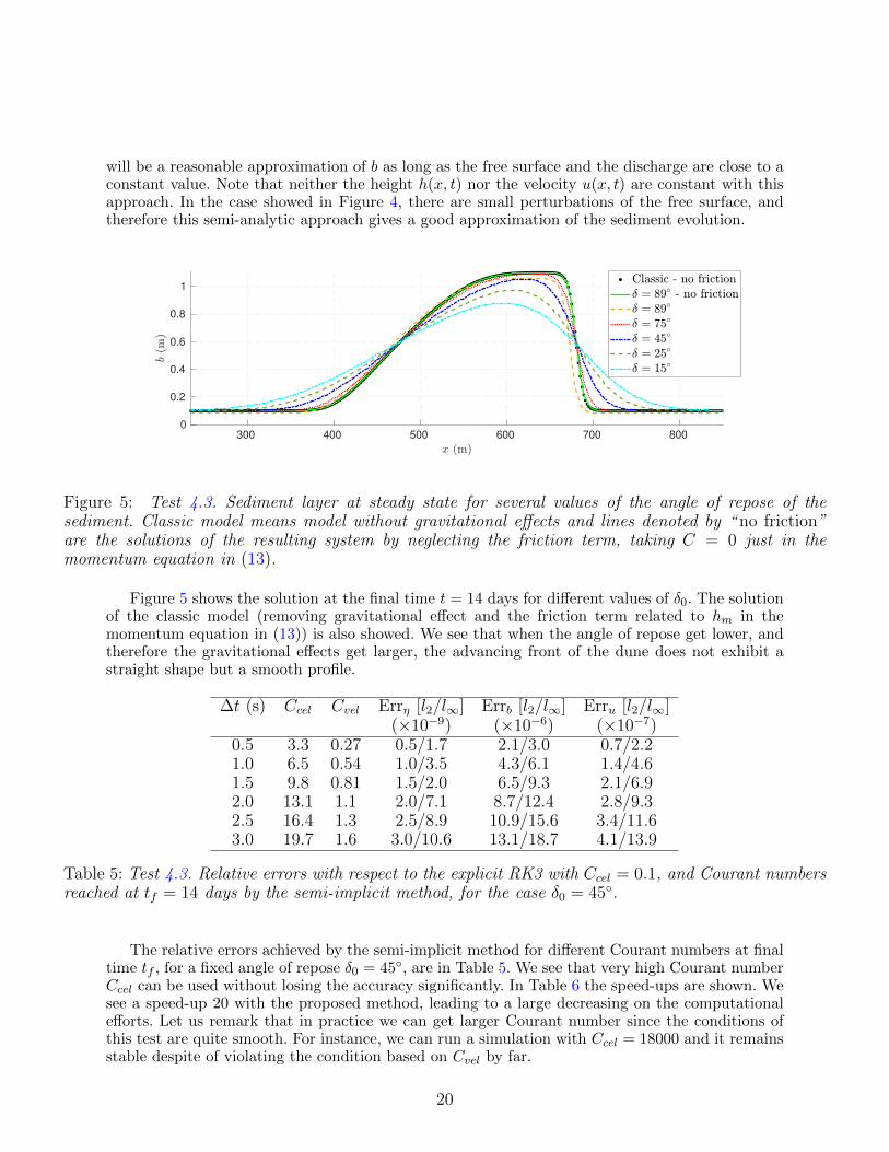
300 400 500 600 700 800

0

0.2

0.4

0.6

0.8

1

Figure 5: Test 4.3. Sediment layer at steady state for several values of the angle of repose of thesediment. Classic model means model without gravitational effects and lines denoted by “ no friction”are the solutions of the resulting system by neglecting the friction term, taking C = 0 just in themomentum equation in (13).

Figure 5 shows the solution at the final time t = 14 days for different values of δ0. The solutionof the classic model (removing gravitational effect and the friction term related to hm in themomentum equation in (13)) is also showed. We see that when the angle of repose get lower, andtherefore the gravitational effects get larger, the advancing front of the dune does not exhibit astraight shape but a smooth profile.

∆t (s) Ccel Cvel Errη [l2/l∞] Errb [l2/l∞] Erru [l2/l∞](×10−9) (×10−6) (×10−7)

0.5 3.3 0.27 0.5/1.7 2.1/3.0 0.7/2.21.0 6.5 0.54 1.0/3.5 4.3/6.1 1.4/4.61.5 9.8 0.81 1.5/2.0 6.5/9.3 2.1/6.92.0 13.1 1.1 2.0/7.1 8.7/12.4 2.8/9.32.5 16.4 1.3 2.5/8.9 10.9/15.6 3.4/11.63.0 19.7 1.6 3.0/10.6 13.1/18.7 4.1/13.9

Table 5: Test 4.3. Relative errors with respect to the explicit RK3 with Ccel = 0.1, and Courant numbersreached at tf = 14 days by the semi-implicit method, for the case δ0 = 45◦.

The relative errors achieved by the semi-implicit method for different Courant numbers at finaltime tf , for a fixed angle of repose δ0 = 45◦, are in Table 5. We see that very high Courant numberCcel can be used without losing the accuracy significantly. In Table 6 the speed-ups are shown. Wesee a speed-up 20 with the proposed method, leading to a large decreasing on the computationalefforts. Let us remark that in practice we can get larger Courant number since the conditions ofthis test are quite smooth. For instance, we can run a simulation with Ccel = 18000 and it remainsstable despite of violating the condition based on Cvel by far.

20

Method ∆t (s) Ccel Comp. time (s) Speed-up

RK3 - 1.0 1425.7 (23.8 min) 1Θ-method 0.5 3.3 368.14 (6.1 min) 3.9Θ-method 1 6.5 187.73 (3.1 min) 7.6Θ-method 1.5 9.8 134.55 (2.2 min) 10.6Θ-method 2 13.1 106.82 (1.8 min) 13.3Θ-method 2.5 16.4 85.20 (1.4 min) 16.7Θ-method 3 19.7 71.29 (1.2 min) 20.0

Table 6: Test 4.3. Speed-ups reached at final time tf = 14 days with the proposed semi-implicit method,for the case δ0 = 45◦.

4.4 Erosion coast process by a tidal force

In this last test we simulate the erosion in the mouth of a river, as an application of sediment trans-port problems to very slow processes, with a small characteristic time and a huge computationaleffort because of the long-time simulation.

As computational domain we take [0 m, 25000 m] with ∆x = 25 m. The material propertiesare taken as in Subsection 4.2, except for the manning coefficient, which is set as n = 0.018.

The initial condition are given by η0(x) = 15 m, b0(x) = 0.1 m and q0(x) = 8.1 m2/s. Herewe impose subcritical boundary conditions: qext = 8.1 m2/s at x = 0 m and the tidal downstreamcondition ηext(t) = 15 + 3 sin (ωt) m at x = 1000 m, with ω = 2π/(12 · 3600), that is, a 12-hourstide. As final time we take tf = 3974400 s (46 days).

Here we start from a flat erodible bottom, which will be affected by the movement of the freesurface forced by the tide force. In Figure 6 we see the evolution of the bottom, where we observe seethe erosion process and how the upstream condition forces an erosion of the sediment downstream.We see that at final time the thickness of the sediment layer has decreased 10 cm.

0 0.5 1 1.5 2 2.5

104

0

0.02

0.04

0.06

0.08

0.1

Figure 6: Test 4.4. Evolution of the sediment till tf = 46 days (1.5 months), with the Θ-methodand ∆t = 14 s (Ccel ≈ 8.1). Dashed red line is the initial condition, dotted green lines correspond tointermediate times and solid blue line is the solution at final time.

It is remarkable that the value of the discharge is set in order to not having sediment transport

21

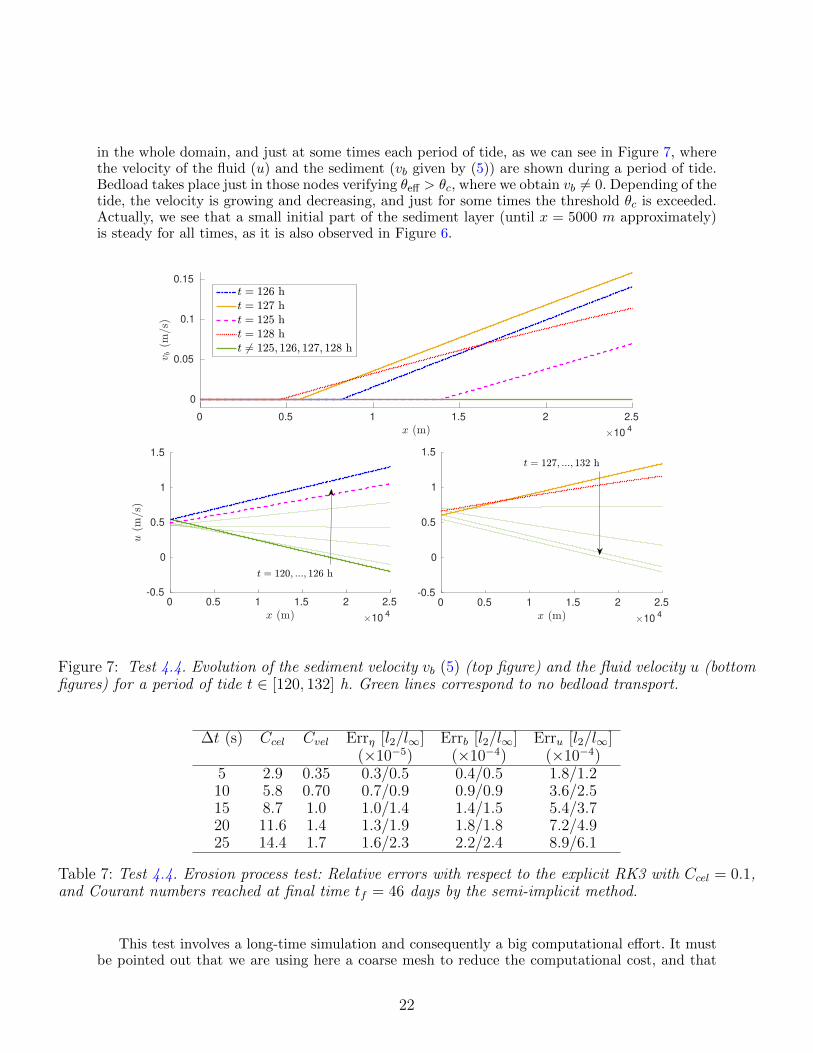
in the whole domain, and just at some times each period of tide, as we can see in Figure 7, wherethe velocity of the fluid (u) and the sediment (vb given by (5)) are shown during a period of tide.Bedload takes place just in those nodes verifying θeff > θc, where we obtain vb 6= 0. Depending of thetide, the velocity is growing and decreasing, and just for some times the threshold θc is exceeded.Actually, we see that a small initial part of the sediment layer (until x = 5000 m approximately)is steady for all times, as it is also observed in Figure 6.

0 0.5 1 1.5 2 2.5

104

0

0.05

0.1

0.15

0 0.5 1 1.5 2 2.5

104

-0.5

0

0.5

1

1.5

0 0.5 1 1.5 2 2.5

104

-0.5

0

0.5

1

1.5

Figure 7: Test 4.4. Evolution of the sediment velocity vb (5) (top figure) and the fluid velocity u (bottomfigures) for a period of tide t ∈ [120, 132] h. Green lines correspond to no bedload transport.

∆t (s) Ccel Cvel Errη [l2/l∞] Errb [l2/l∞] Erru [l2/l∞](×10−5) (×10−4) (×10−4)

5 2.9 0.35 0.3/0.5 0.4/0.5 1.8/1.210 5.8 0.70 0.7/0.9 0.9/0.9 3.6/2.515 8.7 1.0 1.0/1.4 1.4/1.5 5.4/3.720 11.6 1.4 1.3/1.9 1.8/1.8 7.2/4.925 14.4 1.7 1.6/2.3 2.2/2.4 8.9/6.1

Table 7: Test 4.4. Erosion process test: Relative errors with respect to the explicit RK3 with Ccel = 0.1,and Courant numbers reached at final time tf = 46 days by the semi-implicit method.

This test involves a long-time simulation and consequently a big computational effort. It mustbe pointed out that we are using here a coarse mesh to reduce the computational cost, and that

22

Method ∆t (s) Ccel Comp. time (s) Speed-up

RK3 - 0.9 829.3 (13.8 min) 1Θ-method 5 2.9 266.3 (4.4 min) 3.1Θ-method 10 5.8 134.4 (2.2 min) 6.2Θ-method 15 8.7 89.8 (1.5 min) 9.2Θ-method 20 11.6 66.7 (1.1 min) 12.4Θ-method 25 14.4 53.7 (0.89 min) 15.4

Table 8: Test 4.4. Erosion process test: Speed-ups and Courant numbers reached at tf = 46 days by thesemi-implicit method.

our goal is to show the speed-ups reached for the semi-implicit method with respect to the explicitone. The errors made by the theta method with respect to the explicit RK3 method are notsignificative for the current configurations, as we see in Table 7. The Courant numbers and thespeed-ups reached are shown in Table 8. We see that the semi-implicit method is 15 times fasterthan the RK3 method without a significant loss of accuracy, which is an important result. Asin previous test, we want to comment that we can go further in Ccel, this violating the stabilitycondition based on Cvel.

5 Conclusions

An efficient semi-implicit scheme for sediment transport models with gravitational effects undersubcritical regimes has been proposed. For the sake of simplicity, here we have chosen the general-ization of the Ashida & Michiue’s model, which includes gravitational effects through the definitionof τeff. However, this method can be immediately adapted to other models, for both the solid trans-port discharge and the friction model, by redefining Qb in terms of qb in (12). Thus, the proposedapproach can be adapted to a wide range of families of bedload transport models, as presented inSubsection 2.4. We have also shown that the definition of the effective shear stress, τeff, consid-ered in this paper can be seen as an improved formulation of the one proposed by Fowler et al. [19].

An efficient scheme based on the theta method has been proposed following [10], where an it-erative Gauss-Seidel algorithm is needed to solve the resulting linear system on (η, b).For the considered model an explicit expression for steady states verifying Qb = 0. Gravitationalterms play a key role on these steady states, since non-physical solutions are obtained if thesegravitational terms are neglected. This behavior has been shown in the numerical tests, for bothlake at rest and u 6= 0 steady states. In particular, for solutions with u 6= 0 the slope of the steadystates is larger than the angle of repose of the sediment.These gravitational terms also determines the shape of a dune that is swept along by a flow, lead-ing to more realistic (rounded) shapes of the advancing front, where the non-physical shock iscorrected. Here we also have shown that a semi-analytic approach, where η and q are assumed asconstant values, gives reasonable results in this case. Finally, an application to erosion processeshave been performed, where the time of simulation is very large.

In all the cases, we reduce the computational time of simulations with the proposed semi-implicitmethod while the accuracy is not notably degraded.

23

References

[1] K. Ashida and M. Michiue. Study on hydraulic resistance and bed-load transport rate inalluvial streams. Proceedings of the Japan Society of Civil Engineers, 1972(206):59–69, 1972.

[2] R. A. Bagnold. The Flow of Cohesionless Grains in Fluids. Royal Society of London Philo-sophical transactions. Series A. Mathematical and physical sciences, no. 964. Royal Society ofLondon, 1956.

[3] F. Benkhaldoun, M. Seaıd, and S. Sahmim. Mathematical development and verification of afinite volume model for morphodynamic flow applications. Advances in Applied Mathematicsand Mechanics, 3(4):470–492, aug 2011.

[4] M. Bilanceri, F. Beux, I. Elmahi, H. Guillard, and M. V. Salvetti. Linearised implicit time-advancing applied to sediment transport simulations. Research Report RR-7492, INRIA,December 2010.

[5] L. Bonaventura, E. D. Fernandez-Nieto, J. Garres-Dıaz, and G. Narbona-Reina. Multilayershallow water models with locally variable number of layers and semi-implicit time discretiza-tion. Journal of Computational Physics, 364:209–234, 2018.

[6] M. J. Castro Dıaz, E. D. Fernandez-Nieto, and A. M. Ferreiro. Sediment transport modelsin Shallow Water equations and numerical approach by high order finite volume methods.Computers & Fluids, 37(3):299–316, March 2008.

[7] M. J. Castro Dıaz, E. D. Fernandez-Nieto, A. M. Ferreiro, and C. Pares. Two-dimensionalsediment transport models in shallow water equations. A second order finite volume approachon unstructured meshes. Computer Methods in Applied Mechanics and Engineering, 198(33-36):2520–2538, jul 2009.

[8] V. Casulli. Numerical simulation of three-dimensional free surface flow in isopycnal coordi-nates. International Journal of Numerical Methods in Fluids, 25:645 – 658, 1997.

[9] V. Casulli. A semi-implicit numerical method for the free-surface Navier-Stokes equations.International Journal for Numerical Methods in Fluids, 74(8):605–622, nov 2013.

[10] V. Casulli and E. Cattani. Stability, accuracy and efficiency of a semi-implicit method forthree-dimensional shallow water flow. Computers & Mathematics with Applications, 27(4):99– 112, 1994.

[11] V. Casulli and R. T. Cheng. Semi-implicit finite difference methods for three-dimensionalshallow water flow. International Journal for Numerical Methods in Fluids, 15(6):629–648,1992.

[12] V. Casulli and G. S. Stelling. Numerical simulation of 3d quasi-hydrostatic, free-surface flows.Journal of Hydraulic Engineering, 124(7):678–686, 1998.

[13] V. Casulli and R. A. Walters. An unstructured grid, three-dimensional model based on theshallow water equations. International Journal of Numerical Methods in Fluids, 32:331–348,2000.

[14] V. Casulli and P. Zanolli. Semi-implicit numerical modelling of non-hydrostatic free-surfaceflows for environmental problems. Mathematical and Computer Modelling, 36:1131–1149, 2002.

[15] F. Charru. Selection of the ripple length on a granular bed sheared by a liquid flow. Physicsof Fluids, 18:121508, 2006.

[16] F. Exner. Uber die Wechselwirkung zwischen Wasser und Geschiebe in Flussen. Sitzungsber.d. Akad. d. Wiss. pt. IIa. Bd. 134, 1925.

24

[17] R. Fernandez-Luque and R. van Beek. Erosion and transport of bedload sediment. J. Hydraul.Res., 14(2):127–144, 1976.

[18] E. D. Fernandez-Nieto, T. Morales de Luna, G. Narbona-Reina, and J. D. Zabsonre. Formaldeduction of the Saint-Venant–Exner model including arbitrarily sloping sediment beds andassociated energy. ESAIM: Mathematical Modelling and Numerical Analysis, 51(1):115–145,2017.

[19] A. C. Fowler, N. Kopteva, and C. Oakley. The formation of river channel. SIAM J. Appl.Math., 67:1016–1040, 2007.

[20] J. Fredsøe. On the development of dunes in erodible channels. Journal of Fluid Mechanics,64(1):1–16, jun 1974.

[21] G. Garegnani, G. Rosatti, and L. Bonaventura. Free surface flows over mobile bed: mathemat-ical analysis and numerical modeling of coupled and decoupled approaches. Communicationsin Applied and Industrial Mathematics, 1(3), 2011.

[22] G. Garegnani, G. Rosatti, and L. Bonaventura. On the range of validity of the Exner-basedmodels for mobile-bed river flow simulations. Journal of Hydraulic Research, 51:380–391, 2013.

[23] J. Garres-Dıaz and L. Bonaventura. Flexible and efficient discretizations of multilayer modelswith variable density. Applied Mathematics and Computation, 402:126097, aug 2021.

[24] A. J. Grass. Sediment transport by waves and currents. 1981.

[25] P. H. Gunawan, R. Eymard, and S. R. Pudjaprasetya. Staggered scheme for the Exner–ShallowWater equations. Computational Geosciences, 19(6):1197–1206, oct 2015.

[26] L. Hascoet and V. Pascual. TAPENADE 2.1 user’s guide. Technical Report RT-0300, INRIA,2004.

[27] C. A. Kennedy and M. H. Carpenter. Additive Runge-Kutta schemes for convection-diffusion-reaction equations. Applied Numerical Mathematics, 44:139–181, 2003.

[28] A. Kovacs and G. Parker. A new vectorial bedload formulation and its application to the timeevolution of straight river channels. Journal of Fluid Mechanics, 267:153–183, may 1994.

[29] D. K. Lysne. Movement of sand in tunnels. Journal of the Hydraulics Division, 95(6):1835–1846, nov 1969.

[30] E. Meyer-Peter and R. Muller. Formulas for bed-load transport. Rep. 2nd Meet. Int. Assoc.Hydraul. Struct. Res., Stockolm, page 39–64, 1948.

[31] T. Morales de Luna, M. J. Castro Dıaz, and C. Pares Madronal. A duality method for sedimenttransport based on a modified Meyer-Peter & Muller model. Journal of Scientific Computing,48(1-3):258–273, dec 2010.

[32] P. Nielsen. Coastal Bottom Boundary Layers and Sediment Transport. WORLD SCIENTIFIC,jul 1992.

[33] G. Parker, G. Seminara, and L. Solari. Bed load at low shields stress on arbitrarily slopingbeds: Alternative entrainment formulation. Water Resources Research, 39(7), jul 2003.

[34] G. Rosatti, L. Bonaventura, A. Deponti, and G. Garegnani. An accurate and efficient semi-implicit method for section-averaged free-surface flow modelling. International Journal ofNumerical Methods in Fluids, 65:448–473, 2011.

[35] G. Seminara, L. Solari, and G. Parker. Bed load at low shields stress on arbitrarily slopingbeds: Failure of the bagnold hypothesis. Water Resources Research, 38(11):31–1–31–16, nov2002.

25

[36] P. A. Tassi, S. Rhebergen, C. A. Vionnet, and O. Bokhove. A discontinuous Galerkin finiteelement model for river bed evolution under shallow flows. Computer Methods in AppliedMechanics and Engineering, 197(33-40):2930–2947, jun 2008.

[37] L. C. Van Rijn. Sediment Transport, Part I: Bed Load Transport. Journal of HydraulicEngineering, 110(10):1431–1456, 1984.

26