�����������������

Citation: Maaroof, O.W.; Dede,

M.I.C.; Aydin, L. A Robot Arm

Design Optimization Method by

Using a Kinematic Redundancy

Resolution Technique. Robotics 2022,

11, 1. https://doi.org/10.3390/

robotics11010001

Academic Editor: Alessandro

Di Nuovo

Received: 15 November 2021

Accepted: 19 December 2021

Published: 22 December 2021

Publisher’s Note: MDPI stays neutral

with regard to jurisdictional claims in

published maps and institutional affil-

iations.

Copyright: © 2021 by the authors.

Licensee MDPI, Basel, Switzerland.

This article is an open access article

distributed under the terms and

conditions of the Creative Commons

Attribution (CC BY) license (https://

creativecommons.org/licenses/by/

4.0/).

robotics

Article

A Robot Arm Design Optimization Method by Usinga Kinematic Redundancy Resolution Technique

Omar W. Maaroof 1,* , Mehmet Ismet Can Dede 2 and Levent Aydin 3

1 Mechatronics Engineering Department, University of Mosul, Mosul 41002, Iraq2 Department of Mechanical Engineering, Izmir Institute of Technology, Gülbahçe Mahallesi, Urla,

Izmir 35430, Turkey; candede@iyte.edu.tr3 Department of Mechanical Engineering, Izmir Katip Çelebi University, A.O.S.B. Mahallesi, Çigli,

Izmir 35620, Turkey; levent.aydin@ikcu.edu.tr* Correspondence: omarmaaroof@uomosul.edu.iq

Abstract: Redundancy resolution techniques have been widely used for the control of kinematicallyredundant robots. In this work, one of the redundancy resolution techniques is employed in themechanical design optimization of a robot arm. Although the robot arm is non-redundant, theproposed method modifies robot arm kinematics by adding virtual joints to make the robot armkinematically redundant. In the proposed method, a suitable objective function is selected to optimizethe robot arm’s kinematic parameters by enhancing one or more performance indices. Then the robotarm’s end-effector is fixed at critical positions while the redundancy resolution algorithm movesits joints including the virtual joints because of the self-motion of a redundant robot. Hence, theoptimum values of the virtual joints are determined, and the design of the robot arm is modifiedaccordingly. An advantage of this method is the visualization of the changes in the manipulator’sstructure during the optimization process. In this work, as a case study, a passive robotic arm thatis used in a surgical robot system is considered and the task is defined as the determination ofthe optimum base location and the first link’s length. The results indicate the effectiveness of theproposed method.

Keywords: design optimization; redundancy resolution; robot mechanism design; optimizationtechniques; surgical robots

1. Introduction

Optimization methods have been employed in a wide range of areas from economicalsciences to design processes in engineering applications. All optimization techniques de-pend on the numerical and/or algorithmic approach. With the improvement and availabil-ity of powerful computers, many techniques for optimization studies are presented. Suchmethods can be listed as genetic algorithms (GA) [1], Ant Colony Optimization (ACO) [2],and Particle Swarm Optimization (PSO) method [3]. These methods are categorized asmodern and nontraditional optimization methods. However, optimization techniqueshave rewards and drawbacks. Various modifications to improve these techniques havebeen a focus of many studies. The readers are directed to related resources on methods ofoptimization and comparative studies such as the study in [4] as well as the review study ofthe seven stochastic optimization methods that are preferred in optimization of industrialdesigns [5].

All systems that require an optimum design are inherently redundant. In robotics,among the other possible redundancy of components, kinematic redundancy has been anattractive research area since kinematically redundant robot arms may be used to performadditional task/s while performing their main tasks. This is due to the infinite number ofsolutions received for the inverse kinematics analysis of a redundant robot resulting in aninfinite number of configurations of the robot for the same end-effector pose. Consequently,

Robotics 2022, 11, 1. https://doi.org/10.3390/robotics11010001 https://www.mdpi.com/journal/robotics

Robotics 2022, 11, 1 2 of 21

the motions of the links of a robot that are not affecting the motion of the end-effector arenamed “self-motion” by Nakamura [6]. The algorithms that are developed to regulatethe self-motion of the redundant manipulators for a specific aim are called redundancyresolution techniques.

In this study, a design optimization method is formulated specifically for robot ma-nipulators by using Denavit–Hartenberg parameters. The proposed optimization methodadopts a redundancy resolution technique for a kinematically non-redundant manipulator.In this new method, an originally non-redundant manipulator is modified to be a redun-dant manipulator by including virtual joints. Hence, the employment of a redundancyresolution technique is possible for this modified redundant manipulator. The type andlocation of the added virtual joints are selected by the designer for selectively optimizingthe specific parameters of the robot manipulator. The current approach immerses the robotmechanism designer into the optimization process by providing the convergence steps asdesign parameters continuously change to their optimal values. Hence, the optimizationprocess becomes more intuitive to the robot mechanism designer than the optimizationmethods involving randomness. This intuitive approach is our motivation in carrying outthis study and the main novelty of this work.

The structural optimization process is carried out, considering the design constraints,to validate the applicability of this new technique. Design optimization procedures fol-lowed in the design of industrial robot manipulators [7] and the design of haptic devices [8]are utilized in this present work in terms of analyzing the requirements, stating the prob-lem, assigning design constraints, and nominating objective functions. Consequently,performance indices such as manipulability and condition number can be utilized to eval-uate kinematic and/or dynamic performances of manipulators [9]. Specifically, in thispresent work, the objective function that is used in redundancy resolution via null-spaceoptimization is derived by using the modified form of these two indices.

The case scenario selected for this work is the passive arm of a surgical robotic systemcalled NeuRoboScope [10] as shown in Figure 1. In this system, the passive arm is requiredto be backdriven by the surgeon to the designated locations of the surgical workspacewith minimal effort. Therefore, its performance measures related to both kinematic anddynamic manipulability are studied in this paper as objective functions to test the proposedoptimization technique. In the next sections, after a brief review of redundancy resolutiontechniques, the mechanical design optimization technique is described and the passivearm mechanism of the NeuRoboScope system is introduced. Related to this specific casescenario, the design constraints that are used in modifying the problem as the optimizationof a two degree-of-freedom (DoF) planar manipulator are explained. This modification alsofacilitated the understanding and verification of the method described in this paper sincethe two-DoF planar manipulator is an extensively studied manipulator in the literature.The optimization procedure for this case scenario is explained along with the modificationsof the well-known performance indices that are used in this study. Finally, simulations thatare carried out to determine the optimal design of the mechanical structure are presentedand discussions are given on the obtained results.

Robotics 2022, 11, 1 3 of 21Robotics 2022, 10, x FOR PEER REVIEW 3 of 22

Figure 1. The surgical robotic system for minimal invasive pituitary tumor surgery: NeuRoboScope.

2. A Brief Review of Redundancy Resolution Techniques A variety of redundancy resolution methods have been introduced in the literature

such as the Jacobian pseudo-inverse method, weighted pseudo-inverse method, and sin-gularity robustness method (damped least-squares DLS). All those redundancy resolution methods are grouped as Jacobian-based.

By adding constraints in the form of additional tasks to redundancy resolution, the infinite number of solutions is narrowed down to a specific/bounded solution. This is ex-actly equivalent to establishing design constraints in design optimization techniques. To incorporate an additional task, which is usually called the subtask, to the resolution pro-cess of kinematic redundancy, a null-space-based method can be applied. In this method, the gradient of a differentiable objective function is projected in the null-space of the Ja-cobian matrix so that it does not affect the main task. Here, the main task is the task that is usually assigned as the tracking of the end-effector’s motion trajectory.

Another method of redundancy resolution is the decomposition method which de-composes joint-space variables into two groups (two minor Jacobian matrices) as they are related to the main task and the additional task. Afterward, constraint objective equality is utilized as an implicit function to reduce the gradient of optimization objective function [11]. This method has the attribute of eliminating the unnecessary intensive computation of pseudo-inverse which increases the efficiency of calculation time.

In the task augmentation null-space-based method, the Jacobian matrix is extended by the addition of an auxiliary task [12] to result in a square augmented Jacobian matrix. In this method, the pseudo inverse is not to be used [13] and the kinematic solution is no longer redundant.

Multi-task priority is another null-space-based method [14,15]. In this method, other than the Jacobian matrix related to the main task, for each additional subtask, another Jacobian matrix exists. The self-motion of the first subtask is projected to the null-space of the main task’s Jacobian matrix. The motion of the second subtask is projected into the null-space of the first subtask’s Jacobian matrix. In the same means, other lower-order priority subtasks can be embedded in the earlier subtask that has higher priority.

Among possible secondary tasks, the extra DoFs have been used for obstacle avoid-ance in [16], mechanical joint-limit avoidance in [17], minimization of joint velocities and accelerations in [18], and reducing interaction forces in physical human-robot interaction

Figure 1. The surgical robotic system for minimal invasive pituitary tumor surgery: NeuRoboScope.

2. A Brief Review of Redundancy Resolution Techniques

A variety of redundancy resolution methods have been introduced in the literaturesuch as the Jacobian pseudo-inverse method, weighted pseudo-inverse method, and singu-larity robustness method (damped least-squares DLS). All those redundancy resolutionmethods are grouped as Jacobian-based.

By adding constraints in the form of additional tasks to redundancy resolution, theinfinite number of solutions is narrowed down to a specific/bounded solution. This isexactly equivalent to establishing design constraints in design optimization techniques. Toincorporate an additional task, which is usually called the subtask, to the resolution processof kinematic redundancy, a null-space-based method can be applied. In this method, thegradient of a differentiable objective function is projected in the null-space of the Jacobianmatrix so that it does not affect the main task. Here, the main task is the task that is usuallyassigned as the tracking of the end-effector’s motion trajectory.

Another method of redundancy resolution is the decomposition method which de-composes joint-space variables into two groups (two minor Jacobian matrices) as they arerelated to the main task and the additional task. Afterward, constraint objective equality isutilized as an implicit function to reduce the gradient of optimization objective function [11].This method has the attribute of eliminating the unnecessary intensive computation ofpseudo-inverse which increases the efficiency of calculation time.

In the task augmentation null-space-based method, the Jacobian matrix is extendedby the addition of an auxiliary task [12] to result in a square augmented Jacobian matrix.In this method, the pseudo inverse is not to be used [13] and the kinematic solution is nolonger redundant.

Multi-task priority is another null-space-based method [14,15]. In this method, otherthan the Jacobian matrix related to the main task, for each additional subtask, anotherJacobian matrix exists. The self-motion of the first subtask is projected to the null-spaceof the main task’s Jacobian matrix. The motion of the second subtask is projected into thenull-space of the first subtask’s Jacobian matrix. In the same means, other lower-orderpriority subtasks can be embedded in the earlier subtask that has higher priority.

Among possible secondary tasks, the extra DoFs have been used for obstacle avoid-ance in [16], mechanical joint-limit avoidance in [17], minimization of joint velocities andaccelerations in [18], and reducing interaction forces in physical human-robot interaction

Robotics 2022, 11, 1 4 of 21

in [19]. In [20], the manipulability measure was used, and dynamic manipulability wasintroduced in [21]. Most methods for resolving redundancy in manipulation involve defin-ing an objective function to satisfy specific additional tasks. In accordance, in the proposedoptimization technique presented in this paper, those objective functions are used as po-tential performance indices to assign design constraints in the optimization problems forstructural design of manipulators.

3. Description of the New Mechanical Design Optimization Method forRobot Manipulators

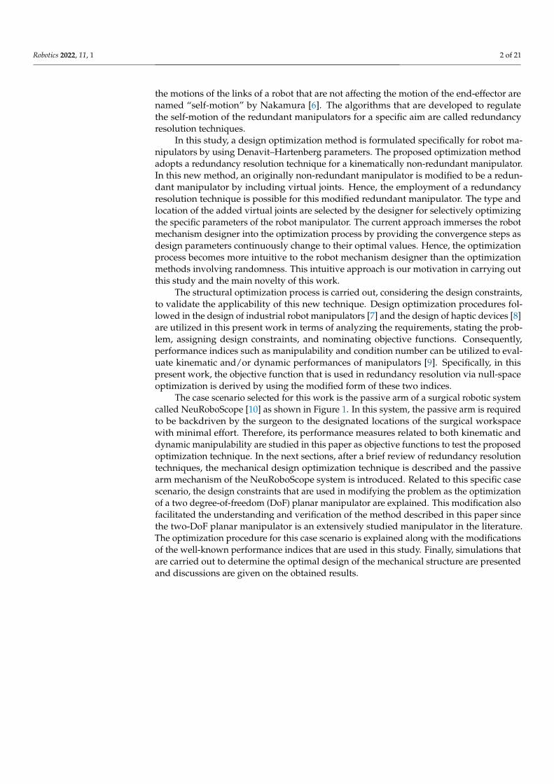
To resolve the redundancy in robot manipulators, first, the manipulator has to bekinematically redundant with respect to the requirements of the task. That is the DoF ofthe manipulator n should be higher than the DoF needed for the task m. In the proposedoptimization method, if n = m, by including p number of virtual joints, the modified robotarm has n + p DoF and becomes a redundant one. The additional virtual joint variablesrepresent the design parameters of a manipulator. In the structural synthesis of a robotarm, design parameter/s can be any Denavit–Hartenberg (DH) [22] parameter/s shown inFigure 2 other than the joint variable. Hence, (1) for link k that is connected to link k− 1 viaa revolute joint, the possible design parameters are the effective link length ak, the twistangle αk and the relative offset between the two links defined along the revolute joint’s axisof rotation dk (2) for link k that is connected to link k− 1 via a prismatic joint, the possibledesign parameters are the effective link length ak, the twist angle αk and the relative rotationbetween the two links defined about the prismatic joint’s motion axis passing from the DHjoint center θk. When a virtual joint is included in the manipulator’s mechanism to changethe design parameter/s, the self-motion of the robot arm becomes a consequence of thechange of the selected design parameter/s.

Robotics 2022, 10, x FOR PEER REVIEW 4 of 22

in [19]. In [20], the manipulability measure was used, and dynamic manipulability was introduced in [21]. Most methods for resolving redundancy in manipulation involve de-fining an objective function to satisfy specific additional tasks. In accordance, in the pro-posed optimization technique presented in this paper, those objective functions are used as potential performance indices to assign design constraints in the optimization problems for structural design of manipulators.

3. Description of the New Mechanical Design Optimization Method for Robot Manip-ulators

To resolve the redundancy in robot manipulators, first, the manipulator has to be kinematically redundant with respect to the requirements of the task. That is the DoF of the manipulator 𝑛 should be higher than the DoF needed for the task 𝑚. In the proposed optimization method, if 𝑛 = 𝑚, by including 𝑝 number of virtual joints, the modified robot arm has 𝑛 + 𝑝 DoF and becomes a redundant one. The additional virtual joint var-iables represent the design parameters of a manipulator. In the structural synthesis of a robot arm, design parameter/s can be any Denavit–Hartenberg (DH) [22] parameter/s shown in Figure 2 other than the joint variable. Hence, (1) for link 𝑘 that is connected to link 𝑘 − 1 via a revolute joint, the possible design parameters are the effective link length 𝑎 , the twist angle 𝛼 and the relative offset between the two links defined along the revolute joint’s axis of rotation 𝑑 (2) for link 𝑘 that is connected to link 𝑘 − 1 via a prismatic joint, the possible design parameters are the effective link length 𝑎 , the twist angle 𝛼 and the relative rotation between the two links defined about the prismatic joint’s motion axis passing from the DH joint center 𝜃 . When a virtual joint is included in the manipulator’s mechanism to change the design parameter/s, the self-motion of the robot arm becomes a consequence of the change of the selected design parameter/s.

Figure 2. Possible design parameters defined with respect to a modified DH convention.

As a next step, a suitable objective function to be minimized or maximized should be selected to optimize the selected design parameters, which are, in this case, the added virtual joints. The objective functions are generally selected to represent a performance index defined for robot manipulators such as manipulability or condition number. How-ever, the designer can also formulate an objective function based on the requirements of the manipulator’s task.

The aim in this method is to calculate the optimal values of the virtual joints by max-imizing or minimizing the objective function via a redundancy resolution algorithm and thus, selecting optimal design parameters. However, for the redundancy resolution algo-rithm to control the self-motion of the manipulator, joints should move at a finite rate.

Figure 2. Possible design parameters defined with respect to a modified DH convention.

As a next step, a suitable objective function to be minimized or maximized shouldbe selected to optimize the selected design parameters, which are, in this case, the addedvirtual joints. The objective functions are generally selected to represent a performanceindex defined for robot manipulators such as manipulability or condition number. However,the designer can also formulate an objective function based on the requirements of themanipulator’s task.

The aim in this method is to calculate the optimal values of the virtual joints bymaximizing or minimizing the objective function via a redundancy resolution algorithmand thus, selecting optimal design parameters. However, for the redundancy resolutionalgorithm to control the self-motion of the manipulator, joints should move at a finiterate. This means enough time should be provided during the optimization so that the self-

Robotics 2022, 11, 1 5 of 21

motion of the manipulator is completed, and the optimal values of the design parametersare obtained. To ensure that there is enough time for self-motion of the manipulatorto be completed, the end-effector of the manipulator is fixed to a specific pose and theconvergence of the parameters is observed. This specific pose may be selected as a criticalor most visited pose of the manipulator. In this way it is possible to observe the changesin the design parameters as the optimization process is carried out. Consequently, thedesigner can gain insight into the effect of the design parameters on the performance ofthe manipulator.

4. Optimization Methodology Described for the Passive Arm of the NeuRoboScopeSystem

In this section, the robot manipulator’s mechanism that is selected as a case study isintroduced. Later, the structural synthesis optimization of this robot arm mechanism isexplained by defining the specific optimization procedure applied in this case scenario.

4.1. Mechanism of the Robotic Manipulator and the Description of the Case Scenario

The manipulator that is considered for the case scenario is designed as a passive armof the NeuRoboScope surgical system (Figure 1). The NeuRoboScope system is designatedto work alongside the surgeon assisting him/her by handling the camera system, theendoscope, throughout the surgery. The passive arm carries an active arm mounted on itslast link and the endoscope is attached to the active arm.

The passive arm has six revolute joints that are not actuated. The surgeon is expectedto backdrive the passive arm to locate the active arm at some desired poses during thesurgery. Accordingly, the joints of the passive arm are equipped with brake systems tomaintain their angular positions when desired by the surgeon.

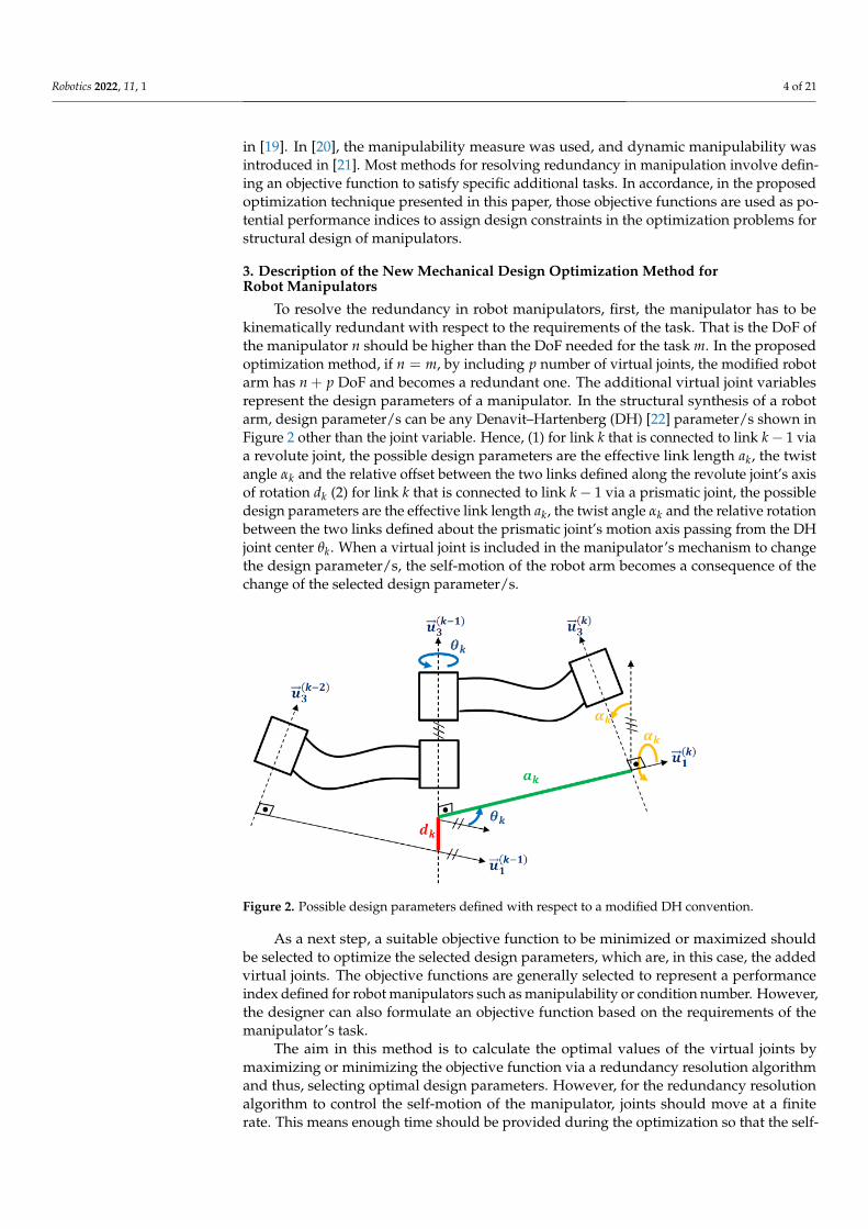
The passive arm’s kinematic architecture is shown in Figure 3. The first two revolutejoints are for the planar motion on the horizontal plane. Third and fourth revolute jointshave axes parallel to the horizontal plane and they are interrelated to each other witha parallelogram loop so that θ3 + θ4 = 2π. The other three joints compose the wristmechanism that is responsible for adjusting the orientation of the active arm’s base locatedat the last link of the passive arm. In Figure 3, MP is identified as the manipulation point atwhich the ease of manipulation of the passive arm is designated to be calculated.

Robotics 2022, 10, x FOR PEER REVIEW 6 of 22

Figure 3. Kinematic scheme of the passive robot arm.

The position of MP is assigned as the maneuvering point which is essential for being a critical consideration for optimization. �� = 𝑎 𝑢( ) + 𝑑 ��( ) + 𝑎 𝑢( ) + 𝑎 𝑢( ) + 𝑎 𝑢( ) (1)

In Equation (1), 𝑑 , 𝑎 , 𝑎 , and 𝑎 are assigned as fixed parameters. The only varia-ble is the design parameter that is selected for this optimization study which is the effec-tive link length of the first link, 𝑎 .

The joint variables are 𝜃 , 𝜃 , 𝜃 , and 𝜃 , three of which are independent parameters so that the position in the Cartesian space is to be considered as moving on a horizontal plane as related to 𝜃 and 𝜃 . Apart from that, 𝜃 is related to the vertical motion and it is selected as a constant value as explained previously. In this way, the passive arm is reduced into a planar revolute-revolute (RR) manipulator. Consequently, the length of the new second link is calculated as 𝑎∗ = 𝑎 + 𝑎 + 𝑎 cos 𝜃 .

The position of the MP is assigned as a constraint for design. Concerning that this position on the horizontal plane and the base of the passive arm is fixed at a specific point on the surgery table, two possible configurations can be calculated as elbow-up and el-bow-down. Any one of the two solutions can be selected to find the initial position for each of 𝜃 and 𝜃 during the optimization study. The inverse kinematics solutions are not presented here since it is trivial for a planar two DoF revolute-jointed arm.

For verifying and testing the objective function on the actual passive arm, the original Jacobian matrix is a 𝐽 ∈ ℜ × matrix for the planar arm with two DoF. However, for op-timization study, virtual joints are added to the original passive arm and the Jacobian matrix is modified as 𝐽 × ∈ ℜ × and 𝐽 × ∈ ℜ × . The case with the two virtual joints (𝐽 × ) includes a prismatic joint acting along the y-axis and its positive direction motion is defined along −𝑢( ) axis by a virtual joint parameter 𝑌 . The other virtual joint in the two-virtual joint case (𝐽 × ) and the single-virtual joint case (𝐽 × ) is the prismatic joint included to change the effective link length, 𝑎 . The dimension of the Jacobian matrix is related to the DoF of the workspace and DoF of the original or modified passive arm. In Equations (2)–(4), Jacobian matrices with two virtual joints, one virtual joint, and no vir-tual joints are presented, respectively. 𝐽 × = 0 𝑐1 −𝑎 𝑠1 − (𝑎 + 𝑎 + 𝑎 𝑐3)𝑠12 −(𝑎 + 𝑎 + 𝑎 𝑐3)𝑠12−1 𝑠1 𝑎 𝑐1 + (𝑎 + 𝑎 + 𝑎 𝑐3)𝑐12 (𝑎 + 𝑎 + 𝑎 𝑐3)𝑐12 (2)

Figure 3. Kinematic scheme of the passive robot arm.

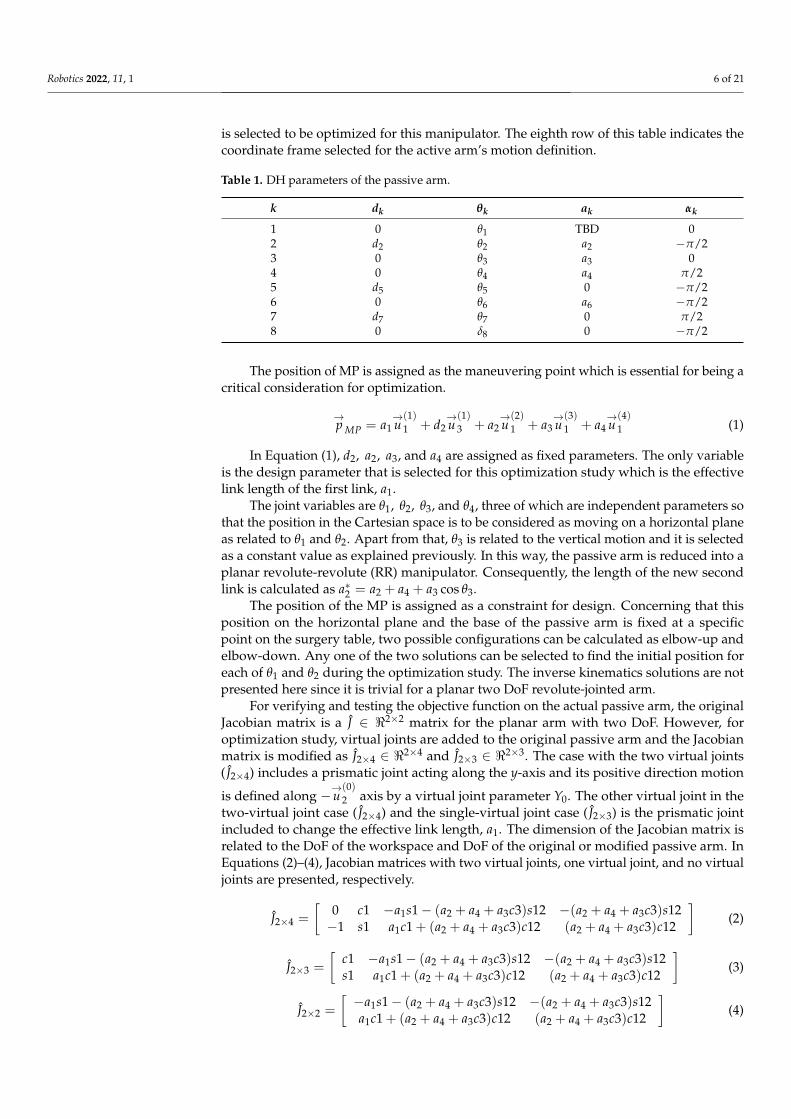
DH parameters of the passive arm are provided in Table 1. In this table, a1 length iskept as to be designed (TBD) on purpose since in the case study, this is the link length that

Robotics 2022, 11, 1 6 of 21

is selected to be optimized for this manipulator. The eighth row of this table indicates thecoordinate frame selected for the active arm’s motion definition.

Table 1. DH parameters of the passive arm.

k dk θk ak αk

1 0 θ1 TBD 02 d2 θ2 a2 −π/23 0 θ3 a3 04 0 θ4 a4 π/25 d5 θ5 0 −π/26 0 θ6 a6 −π/27 d7 θ7 0 π/28 0 δ8 0 −π/2

The position of MP is assigned as the maneuvering point which is essential for being acritical consideration for optimization.

→p MP = a1

→u(1)1 + d2

→u(1)3 + a2

→u(2)1 + a3

→u(3)1 + a4

→u(4)1 (1)

In Equation (1), d2, a2, a3, and a4 are assigned as fixed parameters. The only variableis the design parameter that is selected for this optimization study which is the effectivelink length of the first link, a1.

The joint variables are θ1, θ2, θ3, and θ4, three of which are independent parameters sothat the position in the Cartesian space is to be considered as moving on a horizontal planeas related to θ1 and θ2. Apart from that, θ3 is related to the vertical motion and it is selectedas a constant value as explained previously. In this way, the passive arm is reduced into aplanar revolute-revolute (RR) manipulator. Consequently, the length of the new secondlink is calculated as a∗2 = a2 + a4 + a3 cos θ3.

The position of the MP is assigned as a constraint for design. Concerning that thisposition on the horizontal plane and the base of the passive arm is fixed at a specificpoint on the surgery table, two possible configurations can be calculated as elbow-up andelbow-down. Any one of the two solutions can be selected to find the initial position foreach of θ1 and θ2 during the optimization study. The inverse kinematics solutions are notpresented here since it is trivial for a planar two DoF revolute-jointed arm.

For verifying and testing the objective function on the actual passive arm, the originalJacobian matrix is a J ∈ <2×2 matrix for the planar arm with two DoF. However, foroptimization study, virtual joints are added to the original passive arm and the Jacobianmatrix is modified as J2×4 ∈ <2×4 and J2×3 ∈ <2×3. The case with the two virtual joints( J2×4) includes a prismatic joint acting along the y-axis and its positive direction motion

is defined along −→u(0)2 axis by a virtual joint parameter Y0. The other virtual joint in the

two-virtual joint case ( J2×4) and the single-virtual joint case ( J2×3) is the prismatic jointincluded to change the effective link length, a1. The dimension of the Jacobian matrix isrelated to the DoF of the workspace and DoF of the original or modified passive arm. InEquations (2)–(4), Jacobian matrices with two virtual joints, one virtual joint, and no virtualjoints are presented, respectively.

J2×4 =

[0 c1 −a1s1− (a2 + a4 + a3c3)s12 −(a2 + a4 + a3c3)s12−1 s1 a1c1 + (a2 + a4 + a3c3)c12 (a2 + a4 + a3c3)c12

](2)

J2×3 =

[c1 −a1s1− (a2 + a4 + a3c3)s12 −(a2 + a4 + a3c3)s12s1 a1c1 + (a2 + a4 + a3c3)c12 (a2 + a4 + a3c3)c12

](3)

J2×2 =

[−a1s1− (a2 + a4 + a3c3)s12 −(a2 + a4 + a3c3)s12a1c1 + (a2 + a4 + a3c3)c12 (a2 + a4 + a3c3)c12

](4)

Robotics 2022, 11, 1 7 of 21

In the equations above, sk = sin θk and ck = cos θk for k = 1, 2, 3, and s12 = sin(θ1 + θ2)and c12 = cos(θ1 + θ2).

4.2. Design Optimization Constraints

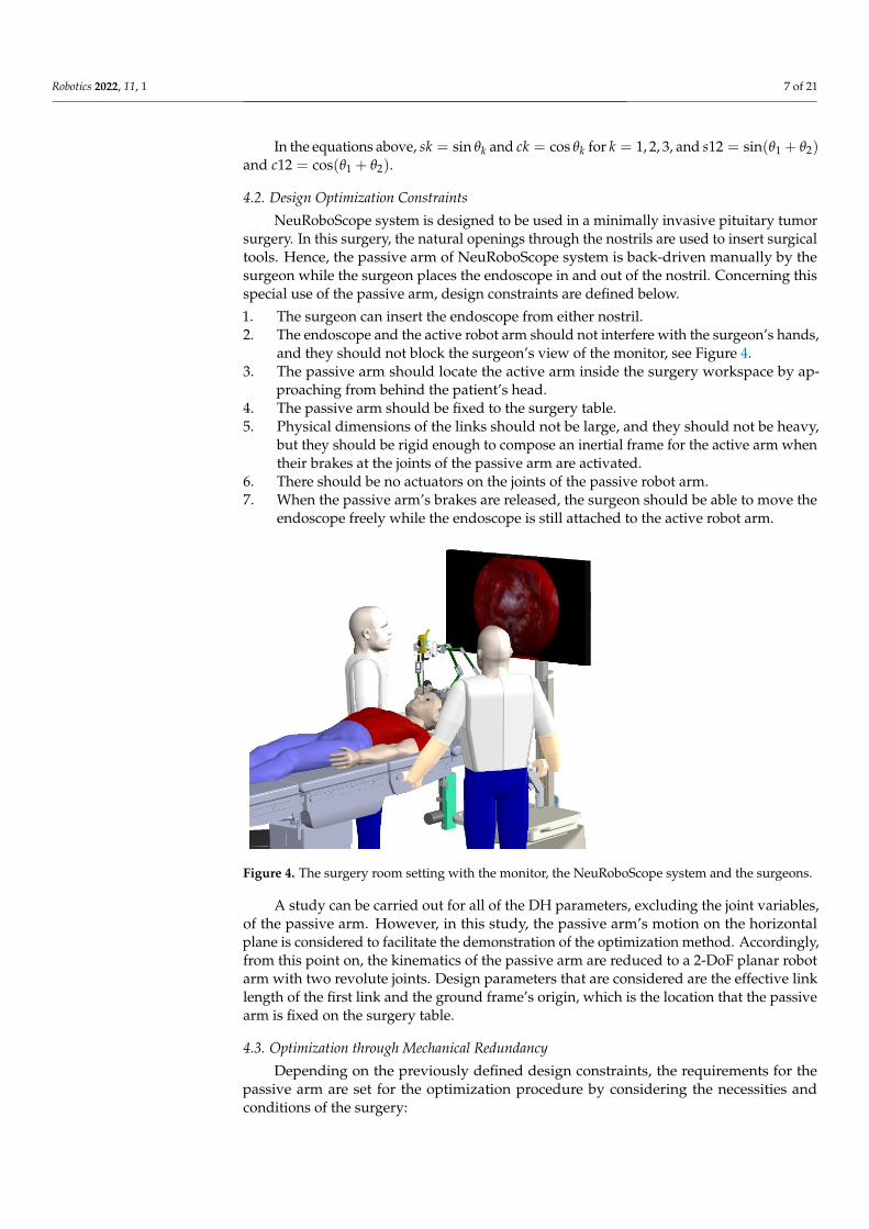
NeuRoboScope system is designed to be used in a minimally invasive pituitary tumorsurgery. In this surgery, the natural openings through the nostrils are used to insert surgicaltools. Hence, the passive arm of NeuRoboScope system is back-driven manually by thesurgeon while the surgeon places the endoscope in and out of the nostril. Concerning thisspecial use of the passive arm, design constraints are defined below.

1. The surgeon can insert the endoscope from either nostril.2. The endoscope and the active robot arm should not interfere with the surgeon’s hands,

and they should not block the surgeon’s view of the monitor, see Figure 4.3. The passive arm should locate the active arm inside the surgery workspace by ap-

proaching from behind the patient’s head.4. The passive arm should be fixed to the surgery table.5. Physical dimensions of the links should not be large, and they should not be heavy,

but they should be rigid enough to compose an inertial frame for the active arm whentheir brakes at the joints of the passive arm are activated.

6. There should be no actuators on the joints of the passive robot arm.7. When the passive arm’s brakes are released, the surgeon should be able to move the

endoscope freely while the endoscope is still attached to the active robot arm.

Robotics 2022, 10, x FOR PEER REVIEW 7 of 22

𝐽 × = 𝑐1 −𝑎 𝑠1 − (𝑎 + 𝑎 + 𝑎 𝑐3)𝑠12 −(𝑎 + 𝑎 + 𝑎 𝑐3)𝑠12𝑠1 𝑎 𝑐1 + (𝑎 + 𝑎 + 𝑎 𝑐3)𝑐12 (𝑎 + 𝑎 + 𝑎 𝑐3)𝑐12 (3)

𝐽 × = −𝑎 𝑠1 − (𝑎 + 𝑎 + 𝑎 𝑐3)𝑠12 −(𝑎 + 𝑎 + 𝑎 𝑐3)𝑠12𝑎 𝑐1 + (𝑎 + 𝑎 + 𝑎 𝑐3)𝑐12 (𝑎 + 𝑎 + 𝑎 𝑐3)𝑐12 (4)

In the equations above, 𝑠𝑘 = 𝑠𝑖𝑛 𝜃 and 𝑐𝑘 = 𝑐𝑜𝑠 𝜃 for 𝑘 = 1,2,3 , and 𝑠12 =𝑠𝑖𝑛(𝜃 + 𝜃 ) and 𝑐12 = 𝑐𝑜𝑠(𝜃 + 𝜃 ).

4.2. Design Optimization Constraints NeuRoboScope system is designed to be used in a minimally invasive pituitary tu-

mor surgery. In this surgery, the natural openings through the nostrils are used to insert surgical tools. Hence, the passive arm of NeuRoboScope system is back-driven manually by the surgeon while the surgeon places the endoscope in and out of the nostril. Concern-ing this special use of the passive arm, design constraints are defined below. 1. The surgeon can insert the endoscope from either nostril. 2. The endoscope and the active robot arm should not interfere with the surgeon’s

hands, and they should not block the surgeon’s view of the monitor, see Figure 4. 3. The passive arm should locate the active arm inside the surgery workspace by ap-

proaching from behind the patient’s head. 4. The passive arm should be fixed to the surgery table. 5. Physical dimensions of the links should not be large, and they should not be heavy,

but they should be rigid enough to compose an inertial frame for the active arm when their brakes at the joints of the passive arm are activated.

6. There should be no actuators on the joints of the passive robot arm. 7. When the passive arm’s brakes are released, the surgeon should be able to move the

endoscope freely while the endoscope is still attached to the active robot arm.

Figure 4. The surgery room setting with the monitor, the NeuRoboScope system and the surgeons.

A study can be carried out for all of the DH parameters, excluding the joint variables, of the passive arm. However, in this study, the passive arm’s motion on the horizontal plane is considered to facilitate the demonstration of the optimization method. Accord-ingly, from this point on, the kinematics of the passive arm are reduced to a 2-DoF planar robot arm with two revolute joints. Design parameters that are considered are the effective link length of the first link and the ground frame’s origin, which is the location that the passive arm is fixed on the surgery table.

Figure 4. The surgery room setting with the monitor, the NeuRoboScope system and the surgeons.

A study can be carried out for all of the DH parameters, excluding the joint variables,of the passive arm. However, in this study, the passive arm’s motion on the horizontalplane is considered to facilitate the demonstration of the optimization method. Accordingly,from this point on, the kinematics of the passive arm are reduced to a 2-DoF planar robotarm with two revolute joints. Design parameters that are considered are the effective linklength of the first link and the ground frame’s origin, which is the location that the passivearm is fixed on the surgery table.

4.3. Optimization through Mechanical Redundancy

Depending on the previously defined design constraints, the requirements for thepassive arm are set for the optimization procedure by considering the necessities andconditions of the surgery:

Robotics 2022, 11, 1 8 of 21

1. The surgeon should have minimal effort when he/she intends to push the active robotarm in or away from the surgery zone.

2. The parallelogram loop in the passive robot arm is utilized with no modificationssince it is designed with counter-spring for gravity compensation. This linkage isresponsible for providing vertical motion of the base of the active arm.

3. The optimization is related only to the ease of manipulation only on the horizontal plane.4. The fixing point position on the y-axis (with respect to reference-frame in Figure 5) is

selected as a possible design parameter, which is related to another design parameterthat is the first link’s length.

5. MP position is fixed at the coordinate (−20, −30) cm (which can be considered asan average position of workspace required by the surgeon) relative to the referenceframe in Figure 5.

6. The effective link length of the first link should be limited depending on its manufac-turability, final weight and allowed compliant displacements due to loads.

7. The linear density of the first link is taken as follows: mass/length = 1 kg/m.8. The third joint variable θ3 in Figure 3 is fixed at −30◦ which is the condition when the

endoscope is located just above the patient’s nostrils.

Since the objective of the optimization is to ease the manipulation at MP, which is de-noted in Figure 3, forward and inverse kinematics, and the Jacobian matrix calculations arepresented for MP. Hence, these calculations are used for the proposed optimization method.

Robotics 2022, 10, x FOR PEER REVIEW 8 of 22

4.3. Optimization through Mechanical Redundancy Depending on the previously defined design constraints, the requirements for the

passive arm are set for the optimization procedure by considering the necessities and con-ditions of the surgery: 1. The surgeon should have minimal effort when he/she intends to push the active robot

arm in or away from the surgery zone. 2. The parallelogram loop in the passive robot arm is utilized with no modifications

since it is designed with counter-spring for gravity compensation. This linkage is re-sponsible for providing vertical motion of the base of the active arm.

3. The optimization is related only to the ease of manipulation only on the horizontal plane.

4. The fixing point position on the y-axis (with respect to reference-frame in Figure 5) is selected as a possible design parameter, which is related to another design parameter that is the first link’s length.

5. MP position is fixed at the coordinate (−20, −30) cm (which can be considered as an average position of workspace required by the surgeon) relative to the reference frame in Figure 5.

6. The effective link length of the first link should be limited depending on its manu-facturability, final weight and allowed compliant displacements due to loads.

7. The linear density of the first link is taken as follows: mass/length = 1 kg/m. 8. The third joint variable 𝜃 in Figure 3 is fixed at −30° which is the condition when

the endoscope is located just above the patient’s nostrils. Since the objective of the optimization is to ease the manipulation at MP, which is

denoted in Figure 3, forward and inverse kinematics, and the Jacobian matrix calculations are presented for MP. Hence, these calculations are used for the proposed optimization method.

Figure 5. Coordinate system fixed on the surgery table (where the unit vector along the x-axis is 𝑢( ) and the unit vector along the y-axis is 𝑢( )). 5. Implementation of the New Optimization Strategy

When there is kinematic redundancy, there is a free motion of the mechanism even if the end-effector is fixed. This so-called self-motion happens in the null space of the Ja-cobian matrix. In the implementation of the proposed optimization strategy, this property is used. However, to use this property, the non-redundant passive arm must be modified to have more joints.

For the case with two virtual joints, the DoF of the RR planar arm is increased by 2. Consequently, a 4-DoF PRPR planar arm operating for a 2-DoF planar task is formed.

Figure 5. Coordinate system fixed on the surgery table (where the unit vector along the x-axis is→u(0)1

and the unit vector along the y-axis is→u(0)2 ).

5. Implementation of the New Optimization Strategy

When there is kinematic redundancy, there is a free motion of the mechanism even ifthe end-effector is fixed. This so-called self-motion happens in the null space of the Jacobianmatrix. In the implementation of the proposed optimization strategy, this property is used.However, to use this property, the non-redundant passive arm must be modified to havemore joints.

For the case with two virtual joints, the DoF of the RR planar arm is increased by 2.Consequently, a 4-DoF PRPR planar arm operating for a 2-DoF planar task is formed. Sincethe objective is to find optimum design parameters, these new joint variables (Y0 and a1)are included in the control of the self-motion of the resultant redundant arm.

Although a designer is free to choose any redundant manipulator controller, a previ-ously designed controller for redundant robot manipulators is utilized for this optimizationtask [18]. However, only the kinematic part of this controller is used in this work. Thiscontroller is used to control both the main task in task-space, earlier defined by the MP

Robotics 2022, 11, 1 9 of 21

point’s position x in horizontal plane, and a desired subtask by adjusting the joints’ motionin the null space.

An error term is defined as e = xd − x as the tracking error, and xd is defined asthe desired position/trajectory in task-space. The designed controller is presented inEquation (5) where Kv and Kp are diagonal constant feedback gain matrices related to theproportional-derivative (PD) controller of the main task.

..q = J+

(..xd + Kv

.e + Kpe−

.J

.q)+

..βN (5)

The column of joint variables in position level are denoted as q ∈ <n, where n, fromnow on, is the summation of actual and virtual joints in this approach. We consider thata vector function z(.) ∈ <n is calculated as a gradient of optimization objective functionf (q) for a specific optimization objective function (which may be time-dependent function,including design constraints, etc.), and joint velocities in the null space are required to trackthe projection of z onto the null space of J. Since In − J+ J projects vectors onto the nullspace of J, this can be formulated in an error signal calculation as presented in Equation (6),which converges to zero. Here, J+ represents the pseudo-inverse of J and In ∈ <n×n is theidentity matrix.

.eN =

(In − J+ J

)z−

.βN (6)

Assuming the manipulator does not go through a singularity condition, it is needed to

design..βN to obtain the desired result for the subtask objective.

..βN is determined as;

..βN =

(In − J+ J

) .z−

(J+

.J J+ + J+

)Jz + KN

.eN (7)

In Equation (7), KN is a diagonal positive definite feedback matrix. This designedcontrol law guarantees that the error will be bounded and converged to zero [18]. Afterthe description of the controller to be used in the proposed optimization method, theperformance indices that are used to formulate the objective function are explained in thenext subsections. It should be noted that instead of the performance metrics mentionedbelow, the objective function can be developed by considering other performance metricsand/or their variations.

5.1. Manipulability Ellipsoid and Singular Value Decomposition (SVD)

Manipulability of a selected point in a mechanical linkage can be represented as ascalar value related to the area/volume of velocity ellipse/ellipsoid calculated at this point.It is first developed in [20] and introduced as a performance index. Since the motionof any point on a mechanical linkage can be related to the motion of the joints by theJacobian matrix, the scalar representation of the manipulability index Mp is provided inthe following equation.

Mp =√

det( J JT) (8)

In addition to the manipulability index shown in Equation (8), another manipulabilitymeasure in Equation (9) was also formulated by Paul and Stevenson [23] as follows

Mp = |det( J)|. (9)

The objective set when using the manipulability index is to maximize this value viachanging the positions of joints by staying inside the null-space when MP is fixed at thedesired position. During this motion, the effective link length of the first link (a1) and theposition of the fixing point of the passive arm (Y0) will be changing to reach the optimumvalue in this optimization.

Robotics 2022, 11, 1 10 of 21

Singular value decomposition on the matrix J JT is used to solve for singular valuesof J, which also represents the semi-axes of manipulability ellipse during the simulation.The rank of J represents the number of singular values, which is two in this case be-cause in the formulation of the objective function, the Jacobian matrix is related to theoriginal manipulator.

5.2. The Modified Condition Number

Another way to represent force/motion relation of a point in the workspace of amechanism is done by a scalar number called condition number [24]. Manipulabilityrepresents ease of manipulation of the end-effector at a certain location of the workspaceand the condition number relates the length of the maximum and minimum axes ofmanipulability ellipse achieved along with different directions at that specific location ofthe end-effector. The condition number is represented by the ratio of the maximum singularvalue to the minimum singular value of the Jacobian matrix, which represents the radii ofthe manipulability ellipse. The distance between any point on the ellipse and its center wasdefined in [25] as the velocity transmission ratio on one specific direction of motion of theend-effector. In an ideal case, the performance index is 1, which means at that specific point,the velocity transmission ratio is the same in all directions and a circle will be representingthe manipulability.

Force condition number and velocity condition number are calculated in similar ways.Salisbury and Craig [24] introduced force condition number as the amplification of therelative force error at the task-space to the relative torque error at the joint-space. WhileMerlet [26] described a velocity condition number using relative motion error in joint-spaceand relative motion error in the task-space.

In this work, the difference between the maximum and minimum singular values ofthe Jacobian matrix (σmax and σmin, respectively) is used instead of the condition numberand it will be referred as the modified condition number from this point on. The objectivefunction shown in Equation (10) is used in the optimization procedure to be minimized toa minimum value or if possible zero value.

Cn = σmax − σmin (10)

5.3. Generalized Inertia Matrix

To include a dynamic orientated design constraint for the design of the passive arm,the dynamic model of the arm is studied via finding its dynamic equation of motion and thegeneralized inertia matrix. This is essential to find the dominant part of design parametersin the relation between the forces displayed at the end-effector and the consequent motionof the manipulator. In this work, since the end-effector is moved at a slow rate, Coriolisand centripetal forces, and the viscous frictional forces are neglected. Consequently, theremaining part of the dynamic equation is shown below.

τ = M..q (11)

In Equation (11), τ is the column of actuator torques/forces acting on the joints and Mis the generalized inertia matrix. To represent Equation (11) in the task-space, where theinteraction is taking place, the task-space forces are mapped to the joint space forces byusing the Jacobian matrix as follows:

τ = JT F. (12)

Here, in Equation (12), F is the external forces acting at the end-effector. For theslow-motion of the end-effector, where

.q→ 0 , we consider

..q = J−1

..x. Subsequently,

JT F = MJ−1..x. (13)

Robotics 2022, 11, 1 11 of 21

As a result of this expression in Equation (13), mapped generalized inertia matrix(mGIM) MG is defined in the task-space as shown in Equation (14).

J−T MJ−1 = MG (14)

The dynamic performance of the passive arm can be represented by the ellipse (in thecase of the 2-DoF manipulator) which can be plotted for the eigenvalues and eigenvectorsof MG matrix [27]. On the other hand, the dynamic manipulability (the determinant ofJ M−1) as defined in [21] by Yoshikawa relates the loads at actuators to the accelerationoutput at end-effector as shown in Equation (15).

..x = J M−1τ (15)

For the design optimization study of the passive arm, the objective is to minimize theresistance shown to the operator during he/she backdrives the arm, which can be termedas the mechanical impedance [28] of the passive arm. By doing so, the end-effector can bemoved freely inside its workspace with minimum force reflected to the user. This can beachieved by either minimizing the determinant of the numerator part of MG in Equation (14)hence the generalized inertia matrix ImN (previously defined as M), and/or maximizingthe determinant of denominator part of MG, which corresponds to the manipulabilityindex ImD since det( JT J) = det( J JT). In this work, the mapped generalized inertia matrixMG and its abovementioned numerator (ImN) and denominator parts (ImD) are used asindicators of the dynamic performance measure while selecting the objective function.

6. Simulation Tests and Results

Two simulation tests are conducted to verify the presented approach. Two designparameters are used for both tests. The Jacobian matrix developed for the MP of theactual passive arm (RR manipulator version) is used to determine the desired objectivefunction that is related to the modified condition number. All tests are carried out in MatlabSimulink setting the fixed step calculation frequency to 100 Hz with an ODE3 solver. Thefixed position of MP is selected as a design constraint on the horizontal planar workspaceat−20, −30 cm for this particular scenario of the presented case study, which is determinedrelative to the frame described in Figure 5. In all the tests, the initial value of the first linkis chosen as a1 = 30 cm and the initial value of fixing position (first joint’s axis location)along the y-axis is selected to be Y0 = 0 cm. The other parameters of the passive arm areassigned as fixed parameters.

6.1. Simulation Test with the Modified Condition Number Performance Index

In this test, the modified condition number and the manipulability index is calculatedto visualize the effect of the optimization. Both the fixing point of the manipulator alongthe y-axis and the first link’s length are selected as design parameters.

By using the modified condition number, which is presented in Equation (10), as theonly performance index in forming the objective function f (q) = −Cn, singular valuesare forced to be equal during the optimization procedure due to the minimization of theobjective function. As a result, the manipulability ellipse is forced to be a circle and therobot arm moves into an isotropic pose as can be seen in Figure 6.

This result is the same result that is presented and discussed in [29]. The obtainedresults are exactly as expected for the isotropic pose. The optimal length of the firstlink came out to be a1 = 38.47 cm which is equal to a1 = a2

√2. The fixing point position

converged to a position at Y0 = −11.57 cm. It is observed in Figure 7 that the manipulabilityindex decreases while the modified condition number index increases which is makingmaximum and minimum singular values to be equal.

Robotics 2022, 11, 1 12 of 21Robotics 2022, 10, x FOR PEER REVIEW 12 of 22

Figure 6. Change of the robot arm structure and the manipulability ellipse (printed in blue color) during the optimization routine by using the modified condition number.

This result is the same result that is presented and discussed in [29]. The obtained results are exactly as expected for the isotropic pose. The optimal length of the first link came out to be 𝑎 = 38.47 cm which is equal to 𝑎 = 𝑎 √2. The fixing point position con-verged to a position at 𝑌 = −11.57 cm. It is observed in Figure 7 that the manipulability index decreases while the modified condition number index increases which is making maximum and minimum singular values to be equal.

Figure 7. Variation of the manipulability index and singular values during the optimization routine by using the modified condition number.

Figure 6. Change of the robot arm structure and the manipulability ellipse (printed in blue color)during the optimization routine by using the modified condition number.

Robotics 2022, 10, x FOR PEER REVIEW 12 of 22

Figure 6. Change of the robot arm structure and the manipulability ellipse (printed in blue color) during the optimization routine by using the modified condition number.

This result is the same result that is presented and discussed in [29]. The obtained results are exactly as expected for the isotropic pose. The optimal length of the first link came out to be 𝑎 = 38.47 cm which is equal to 𝑎 = 𝑎 √2. The fixing point position con-verged to a position at 𝑌 = −11.57 cm. It is observed in Figure 7 that the manipulability index decreases while the modified condition number index increases which is making maximum and minimum singular values to be equal.

Figure 7. Variation of the manipulability index and singular values during the optimization routine by using the modified condition number. Figure 7. Variation of the manipulability index and singular values during the optimization routineby using the modified condition number.

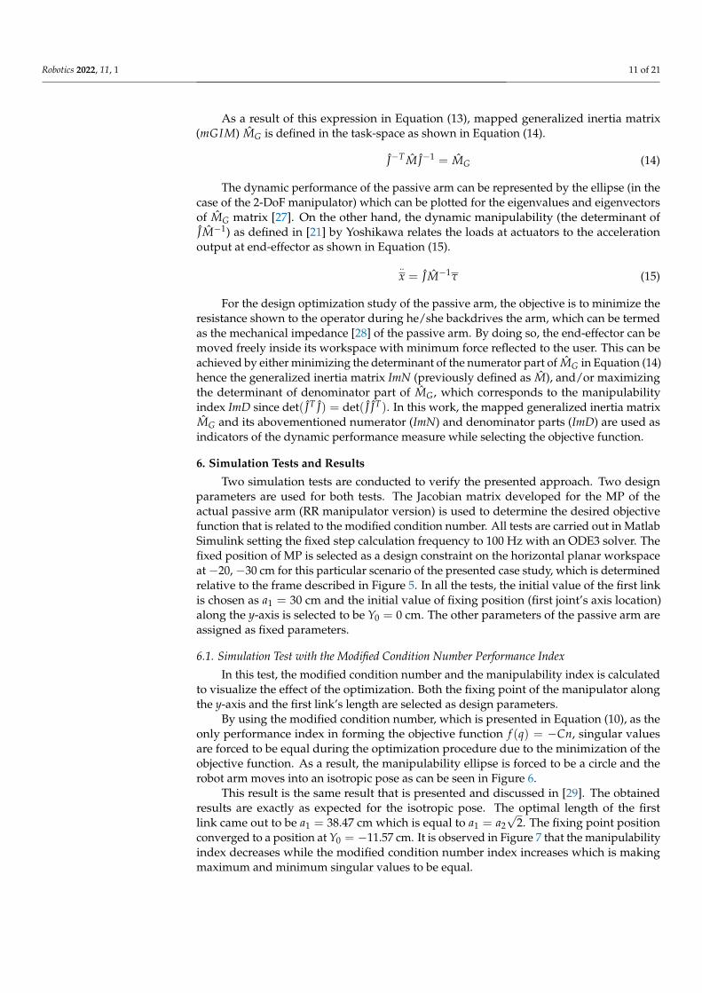
As another consideration of the optimization process, the variation of inertial proper-ties of the manipulator is investigated. In Figure 8a, it can be noticed that the determinantof the mapped generalized inertia matrix (mGIM) is increased because of this optimization.This is due to the increase in the first link length and decrease in overall manipulability.In addition, the determinant of the generalized inertia matrix (the numerator of mGIM) isincreased as can be seen in Figure 8b, which is represented by ImN in this figure. ImD rep-resents manipulability (the denominator of mGIM). As the objective function is minimized,

Robotics 2022, 11, 1 13 of 21

the modified condition number becomes zero since in this work, it is described as the dif-ference between the maximum and minimum singular value of the manipulability matrix.

Robotics 2022, 10, x FOR PEER REVIEW 13 of 22

As another consideration of the optimization process, the variation of inertial prop-erties of the manipulator is investigated. In Figure 8a, it can be noticed that the determi-nant of the mapped generalized inertia matrix (mGIM) is increased because of this opti-mization. This is due to the increase in the first link length and decrease in overall manip-ulability. In addition, the determinant of the generalized inertia matrix (the numerator of mGIM) is increased as can be seen in Figure 8b, which is represented by ImN in this fig-ure. ImD represents manipulability (the denominator of mGIM). As the objective func-tion is minimized, the modified condition number becomes zero since in this work, it is described as the difference between the maximum and minimum singular value of the manipulability matrix.

Figure 8. The optimization procedure with the modified condition number: (a) Variation of the gen-eralized inertia matrix, (b) variation of components of the objective function, (c) variation in the values of design parameters.

During the optimization process, design parameters could converge to constant val-ues. As shown in Figure 8c, the length of the first link is increased due to this optimization, which leads to a decrease in manipulability and as a result increase in the determinant of 𝑚𝐺𝐼𝑀. This can be considered as a drawback but the objective in using the modified con-dition number is to result in an isotropic pose in terms of manipulability index.

6.2. Simulation Test with the Modified Condition Number Performance Index and Generalized Inertia Matrix

In this final test, modified condition number and the numerator part of the mapped generalized inertia matrix, which corresponds to the generalized inertia matrix, are used with selected weights of 𝑤 = 1 and 𝑤 = 2 in forming the objective function, respec-tively. In this way, the objective function is modified to have both the effect of modified condition number and the determinant of the generalized inertia matrix 𝐼𝑚𝑁 as 𝑓(��) =−𝑤 𝐶 − 𝑤 𝐼𝑚𝑁. As a result, shorter length for the first link is obtained and manipulabil-ity ellipse is reshaped as can be noticed in Figure 9.

Figure 8. The optimization procedure with the modified condition number: (a) Variation of thegeneralized inertia matrix, (b) variation of components of the objective function, (c) variation in thevalues of design parameters.

During the optimization process, design parameters could converge to constant values.As shown in Figure 8c, the length of the first link is increased due to this optimization,which leads to a decrease in manipulability and as a result increase in the determinantof mGIM. This can be considered as a drawback but the objective in using the modifiedcondition number is to result in an isotropic pose in terms of manipulability index.

6.2. Simulation Test with the Modified Condition Number Performance Index and GeneralizedInertia Matrix

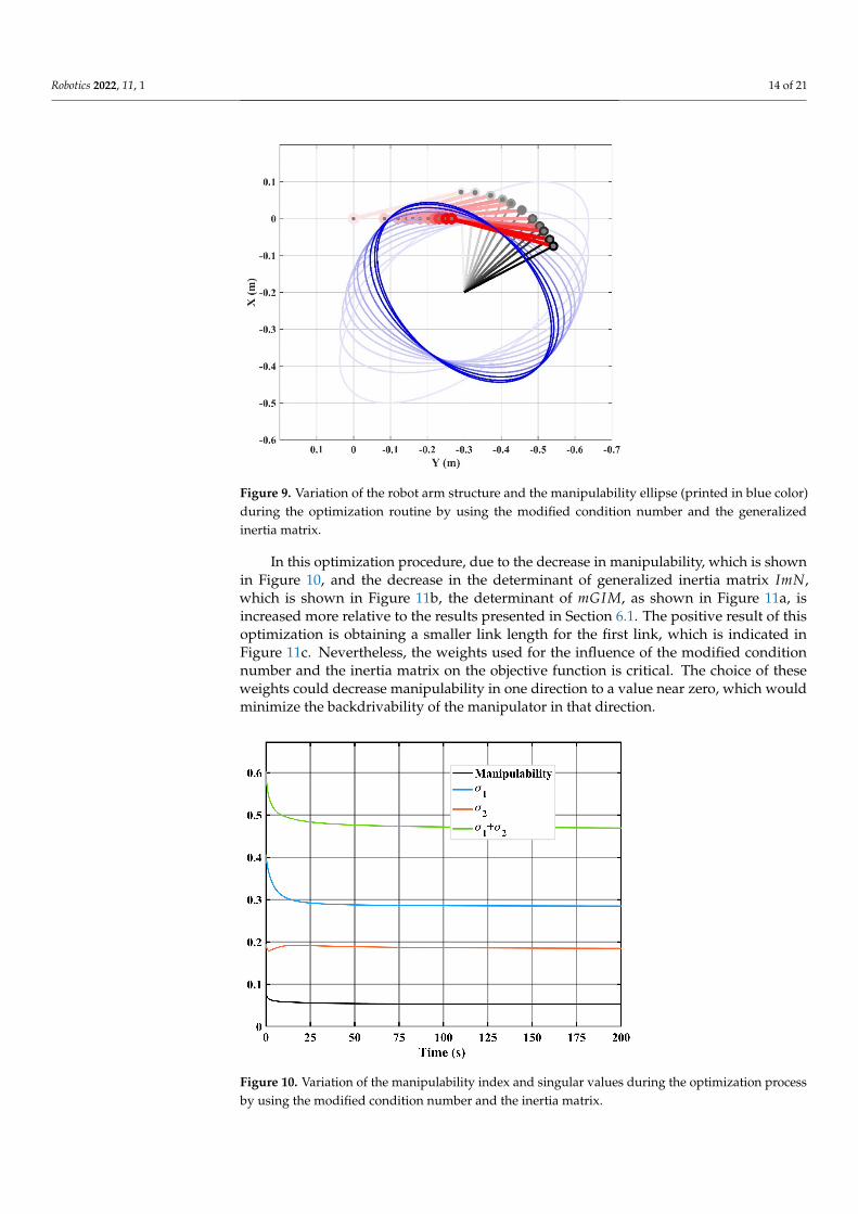
In this final test, modified condition number and the numerator part of the mappedgeneralized inertia matrix, which corresponds to the generalized inertia matrix, are usedwith selected weights of w1 = 1 and w2 = 2 in forming the objective function, respec-tively. In this way, the objective function is modified to have both the effect of mod-ified condition number and the determinant of the generalized inertia matrix ImN asf (q) = −w1Cn − w2 ImN. As a result, shorter length for the first link is obtained and ma-nipulability ellipse is reshaped as can be noticed in Figure 9. In Figures 6 and 9: (1) thered line indicates the first link, and the black line indicates the second link, (2) the jointcenters for the first and second joint are indicated with red and black circles, respectively(3) during the optimization process, the link colors are drawn darker as the links movefrom their initial states to their final states.

Robotics 2022, 11, 1 14 of 21Robotics 2022, 10, x FOR PEER REVIEW 14 of 22

Figure 9. Variation of the robot arm structure and the manipulability ellipse (printed in blue color) during the optimization routine by using the modified condition number and the generalized inertia matrix.

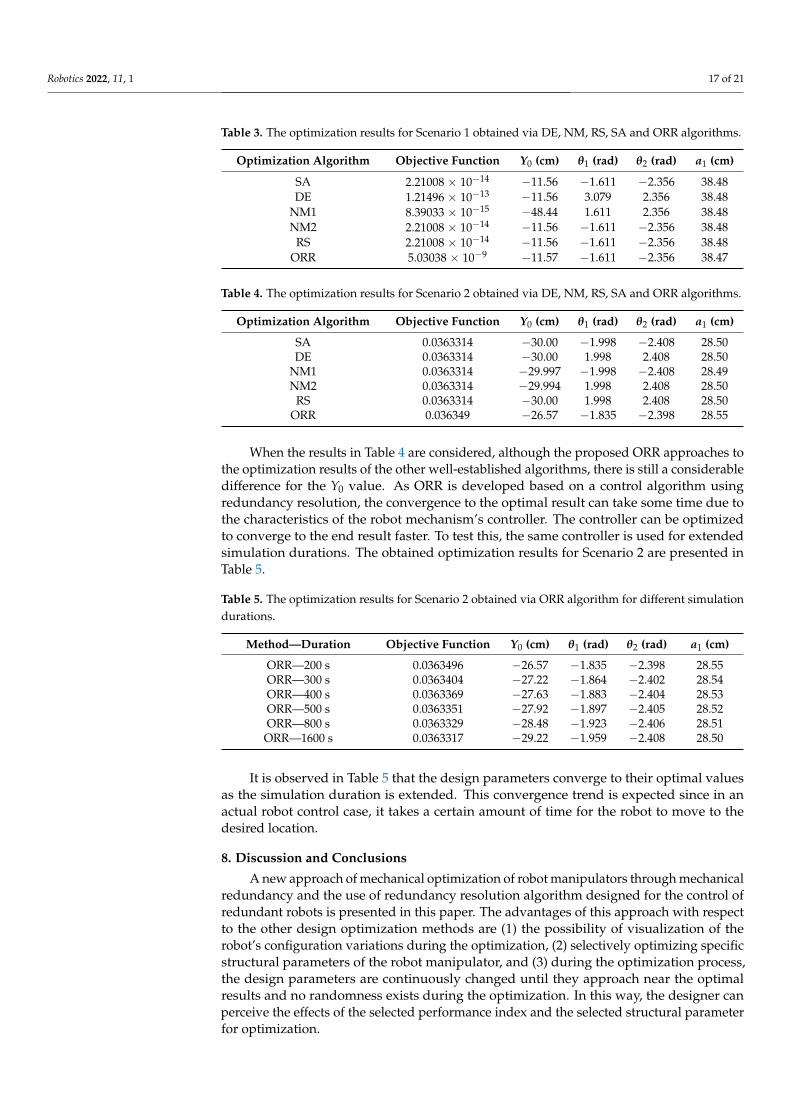
In this optimization procedure, due to the decrease in manipulability, which is shown in Figure 10, and the decrease in the determinant of generalized inertia matrix 𝐼𝑚𝑁, which is shown in Figure 11b, the determinant of 𝑚𝐺𝐼𝑀, as shown in Figure 11a, is increased more relative to the results presented in Section 6.1. The positive result of this optimiza-tion is obtaining a smaller link length for the first link, which is indicated in Figure 11c. Nevertheless, the weights used for the influence of the modified condition number and the inertia matrix on the objective function is critical. The choice of these weights could decrease manipulability in one direction to a value near zero, which would minimize the backdrivability of the manipulator in that direction.

Figure 10. Variation of the manipulability index and singular values during the optimization pro-cess by using the modified condition number and the inertia matrix.

Figure 9. Variation of the robot arm structure and the manipulability ellipse (printed in blue color)during the optimization routine by using the modified condition number and the generalizedinertia matrix.

In this optimization procedure, due to the decrease in manipulability, which is shownin Figure 10, and the decrease in the determinant of generalized inertia matrix ImN,which is shown in Figure 11b, the determinant of mGIM, as shown in Figure 11a, isincreased more relative to the results presented in Section 6.1. The positive result of thisoptimization is obtaining a smaller link length for the first link, which is indicated inFigure 11c. Nevertheless, the weights used for the influence of the modified conditionnumber and the inertia matrix on the objective function is critical. The choice of theseweights could decrease manipulability in one direction to a value near zero, which wouldminimize the backdrivability of the manipulator in that direction.

Robotics 2022, 10, x FOR PEER REVIEW 14 of 22

Figure 9. Variation of the robot arm structure and the manipulability ellipse (printed in blue color) during the optimization routine by using the modified condition number and the generalized inertia matrix.

In this optimization procedure, due to the decrease in manipulability, which is shown in Figure 10, and the decrease in the determinant of generalized inertia matrix 𝐼𝑚𝑁, which is shown in Figure 11b, the determinant of 𝑚𝐺𝐼𝑀, as shown in Figure 11a, is increased more relative to the results presented in Section 6.1. The positive result of this optimiza-tion is obtaining a smaller link length for the first link, which is indicated in Figure 11c. Nevertheless, the weights used for the influence of the modified condition number and the inertia matrix on the objective function is critical. The choice of these weights could decrease manipulability in one direction to a value near zero, which would minimize the backdrivability of the manipulator in that direction.

Figure 10. Variation of the manipulability index and singular values during the optimization pro-cess by using the modified condition number and the inertia matrix.

Figure 10. Variation of the manipulability index and singular values during the optimization processby using the modified condition number and the inertia matrix.

Robotics 2022, 11, 1 15 of 21Robotics 2022, 10, x FOR PEER REVIEW 15 of 22

Figure 11. The optimization procedure with modified condition number and inertia matrix: (a) Var-iation of the generalized inertia matrix, (b) variation of components of the objective function, (c) variation in the values of design parameters.

7. Validation of the Proposed Optimum Design Approach To ease the comparison of our optimization approach, we named our optimization

approach as Optimization via Redundancy Resolution (ORR). To show the accuracy of the proposed optimization approach, we compared the results obtained by stochastic op-timization algorithms Simulated Annealing (SA) algorithm, Differential Evolution (DE) algorithm, Nelder–Mead (NM) algorithm, Random Search (RS) algorithm, based on four different phenomenological search approaches, and that of ORR for the mechanism de-sign problem we defined. Here, the basic rationale for choosing these algorithms for vali-dation is (i) they have proven their reliability in the solution of mathematical optimization problems, which have been used in many different disciplines, (ii) because they have dif-ferent phenomenological bases, a solution alternative that an algorithm might miss can be compensated by this way. At this stage, two different optimization scenarios were de-fined: First, to find the results that minimize only the 𝐶 parameter, and in this context, optimize the parameters 𝑌 , 𝜃 , 𝜃 and 𝑎 under the given nonlinear equality and linear inequality constraints; The second was to define the importance levels of the 𝐶 and 𝐼𝑚𝑁 parameters with the weight values of 𝑤 and 𝑤 , to define a new objective func-tion(𝑤 𝐶 + 𝑤 𝐼𝑚𝑁) and to use the constraints used in the first scenario. Weights are se-lected as 𝑤 = 1 and 𝑤 = 2 in forming the objective function, respectively. The unit for the distances is m and the unit for the angular positions is rad in description of the two optimization scenarios.

Find design variables: 𝑌 , 𝜃 , 𝜃 , 𝑎 Scenario 1: To minimize the objective function: 𝐶 (𝑌 , 𝜃 , 𝜃 , 𝑎 ) Scenario 2: To minimize the objective function: 𝑤 𝐶 (𝑌 , 𝜃 , 𝜃 , 𝑎 ) + 𝑤 𝐼𝑚𝑁(𝑌 , 𝜃 , 𝜃 , 𝑎 )

Figure 11. The optimization procedure with modified condition number and inertia matrix:(a) Variation of the generalized inertia matrix, (b) variation of components of the objective func-tion, (c) variation in the values of design parameters.

7. Validation of the Proposed Optimum Design Approach

To ease the comparison of our optimization approach, we named our optimizationapproach as Optimization via Redundancy Resolution (ORR). To show the accuracy of theproposed optimization approach, we compared the results obtained by stochastic optimiza-tion algorithms Simulated Annealing (SA) algorithm, Differential Evolution (DE) algorithm,Nelder–Mead (NM) algorithm, Random Search (RS) algorithm, based on four differentphenomenological search approaches, and that of ORR for the mechanism design problemwe defined. Here, the basic rationale for choosing these algorithms for validation is (i) theyhave proven their reliability in the solution of mathematical optimization problems, whichhave been used in many different disciplines, (ii) because they have different phenomeno-logical bases, a solution alternative that an algorithm might miss can be compensated bythis way. At this stage, two different optimization scenarios were defined: First, to find theresults that minimize only the Cn parameter, and in this context, optimize the parametersY0, θ1, θ2 and a1 under the given nonlinear equality and linear inequality constraints; Thesecond was to define the importance levels of the Cn and ImN parameters with the weightvalues of w1 and w2, to define a new objective function (w1Cn + w2 ImN) and to use theconstraints used in the first scenario. Weights are selected as w1 = 1 and w2 = 2 in formingthe objective function, respectively. The unit for the distances is m and the unit for theangular positions is rad in description of the two optimization scenarios.

Find design variables: Y0, θ1, θ2, a1Scenario 1:To minimize the objective function: Cn(Y0, θ1, θ2, a1)Scenario 2:To minimize the objective function: w1Cn(Y0, θ1, θ2, a1) + w2 ImN(Y0, θ1, θ2, a1)

Robotics 2022, 11, 1 16 of 21

Subjected to: −1 ≤ Y0 ≤ 0, 0 < a1 < 0.5a2 = 0.350;a3 = 0.216;a4 = 0.05;θ3 = −30π/180;X0 = 0;a∗2 = a2 + a4 + a3 cos θ3;[XMP, YMP] = [− 0.2,−0.3]XMP = a1 cos(θ1) + a∗2 cos(θ1 + θ2);YMP = Y0 + a1 sin(θ1) + a∗2 sin(θ1 + θ2);where

Cn(Y0, θ1, θ2, a1) = 12 (((a2

1 + (a41 + 1.088a3

1 cos(θ2) + 0.592a21 cos2(θ2) + 0.161a1 cos(θ2) + 0.022)0.5

+0.544a1 cos(θ2) + 0.148)

−((a21 − (a4

1 + 1.088a31 cos(θ2) + 0.592a2

1 cos2(θ2) + 0.161a1 cos(θ2) + 0.022)0.5)

+0.544a1 cos(θ2) + 0.148)0.5)0.5)2

ImN(Y0, θ1, θ2, a1) = 0.172707a21 + 0.100746a3

1 − 0.0740175a21 cos2(θ2)

In the Appendix A, summary information about the working logic of the optimizationalgorithms we use for validation is given. For more detailed information, you can refer tothe relevant reference [5].

For the optimization problems solved for the scenarios, the algorithm options given inTable 2 are used.

Table 2. Corresponding options for the optimization algorithms DE, NM, RS, and SA.

Options DE NM RS SA

Crossoverfractions 0.5 - - -

Random Seed 1 5/10 0 2Scaling factor 0.6 - - -

Tolerance 0.001 0.001 0.001 0.001Contact ratio - 0.5 - -Expand ratio - 2.0 - -Reflect ratio - 1.0 - -Shrink ratio - 0.5 - -

Level iterations - - - 50Perturbation

scale - - - 1.0

Penalty Function - - Automatic -Search Points - - 2 -

Method - - Interior Point -

The obtained results using the four well-established optimization algorithm’s resultsare tabulated along with the result obtained by the proposed ORR algorithm. Due to the“RandomSeed” dependency, which is one of the advantages of the NM algorithm, it ispossible to produce alternative results when two different choices (5 and 10) are made forthis problem. Therefore, the results for two version of NM are also presented. Tables 3 and 4present the result obtained for Scenarios 1 and 2, respectively.

In Table 3, the solution obtained in DE algorithm is the positive solution alternativefor the RR manipulator. Therefore, the obtained optimization result in DE is identical to theones obtained via SA, NM2, RS and the proposed ORR algorithm. The result obtained viaNM1 algorithm is different than the other ones. However, when the constraint is narrowedto −0.4 ≤ Y0 ≤ 0, this algorithm also gives the same result with the others.

Robotics 2022, 11, 1 17 of 21

Table 3. The optimization results for Scenario 1 obtained via DE, NM, RS, SA and ORR algorithms.

Optimization Algorithm Objective Function Y0 (cm) θ1 (rad) θ2 (rad) a1 (cm)

SA 2.21008 × 10−14 −11.56 −1.611 −2.356 38.48DE 1.21496 × 10−13 −11.56 3.079 2.356 38.48

NM1 8.39033 × 10−15 −48.44 1.611 2.356 38.48NM2 2.21008 × 10−14 −11.56 −1.611 −2.356 38.48

RS 2.21008 × 10−14 −11.56 −1.611 −2.356 38.48ORR 5.03038 × 10−9 −11.57 −1.611 −2.356 38.47

Table 4. The optimization results for Scenario 2 obtained via DE, NM, RS, SA and ORR algorithms.

Optimization Algorithm Objective Function Y0 (cm) θ1 (rad) θ2 (rad) a1 (cm)

SA 0.0363314 −30.00 −1.998 −2.408 28.50DE 0.0363314 −30.00 1.998 2.408 28.50

NM1 0.0363314 −29.997 −1.998 −2.408 28.49NM2 0.0363314 −29.994 1.998 2.408 28.50

RS 0.0363314 −30.00 1.998 2.408 28.50ORR 0.036349 −26.57 −1.835 −2.398 28.55

When the results in Table 4 are considered, although the proposed ORR approaches tothe optimization results of the other well-established algorithms, there is still a considerabledifference for the Y0 value. As ORR is developed based on a control algorithm usingredundancy resolution, the convergence to the optimal result can take some time due tothe characteristics of the robot mechanism’s controller. The controller can be optimizedto converge to the end result faster. To test this, the same controller is used for extendedsimulation durations. The obtained optimization results for Scenario 2 are presented inTable 5.

Table 5. The optimization results for Scenario 2 obtained via ORR algorithm for different simulationdurations.

Method—Duration Objective Function Y0 (cm) θ1 (rad) θ2 (rad) a1 (cm)

ORR—200 s 0.0363496 −26.57 −1.835 −2.398 28.55ORR—300 s 0.0363404 −27.22 −1.864 −2.402 28.54ORR—400 s 0.0363369 −27.63 −1.883 −2.404 28.53ORR—500 s 0.0363351 −27.92 −1.897 −2.405 28.52ORR—800 s 0.0363329 −28.48 −1.923 −2.406 28.51

ORR—1600 s 0.0363317 −29.22 −1.959 −2.408 28.50

It is observed in Table 5 that the design parameters converge to their optimal valuesas the simulation duration is extended. This convergence trend is expected since in anactual robot control case, it takes a certain amount of time for the robot to move to thedesired location.

8. Discussion and Conclusions

A new approach of mechanical optimization of robot manipulators through mechanicalredundancy and the use of redundancy resolution algorithm designed for the control ofredundant robots is presented in this paper. The advantages of this approach with respectto the other design optimization methods are (1) the possibility of visualization of therobot’s configuration variations during the optimization, (2) selectively optimizing specificstructural parameters of the robot manipulator, and (3) during the optimization process,the design parameters are continuously changed until they approach near the optimalresults and no randomness exists during the optimization. In this way, the designer canperceive the effects of the selected performance index and the selected structural parameterfor optimization.

Robotics 2022, 11, 1 18 of 21

Figure 12 shows the Pareto chart for two performance indices to be minimized (themodified condition number, Cn, and the determinant of the generalized inertia matrix, ImN),by using the selected design parameters within their design limits of Y0 = −0.3 m→ 0 m anda1 = 0 m→ 0.4 m with the discrete step size of 0.01 m. Within these ranges, a Pareto set of961 individual solutions are evaluated for the corresponding performance indices whichare presented with “x” mark on the figure. The distribution of the Pareto set shows theopposing requirements of the two performance indices. In this constrained multi-objectiveoptimization problem, the procedure described in test B is selected for observing the newoptimization method’s performance via the Pareto set. The execution of the proposedoptimization method is printed on the figure which initiates from the point marked withthe red circle and follows the blue line to terminate at the red plus mark. The result ofthe proposed optimization method with two performance indices indicates that its finalresult on the Pareto Front is located at the lower curve in this Pareto set. This demonstratesthat the proposed optimization method guarantees the final solution will be located atthe Pareto Front without setting a stopping criterion as in genetic optimization methods.However, the exact location on the lower curve depends on the weighting values (w1 andw2) which can be selected depending on the desired performance of the robot manipulator.

Robotics 2022, 10, x FOR PEER REVIEW 18 of 22

optimal results and no randomness exists during the optimization. In this way, the de-signer can perceive the effects of the selected performance index and the selected struc-tural parameter for optimization.

Figure 12 shows the Pareto chart for two performance indices to be minimized (the modified condition number, 𝐶 , and the determinant of the generalized inertia matrix, 𝐼𝑚𝑁,) by using the selected design parameters within their design limits of 𝑌 = −0.3 m →0 m and 𝑎 = 0 m → 0.4 m with the discrete step size of 0.01 m. Within these ranges, a Pareto set of 961 individual solutions are evaluated for the corresponding performance indices which are presented with “x” mark on the figure. The distribution of the Pareto set shows the opposing requirements of the two performance indices. In this constrained multi-objective optimization problem, the procedure described in test B is selected for ob-serving the new optimization method’s performance via the Pareto set. The execution of the proposed optimization method is printed on the figure which initiates from the point marked with the red circle and follows the blue line to terminate at the red plus mark. The result of the proposed optimization method with two performance indices indicates that its final result on the Pareto Front is located at the lower curve in this Pareto set. This demonstrates that the proposed optimization method guarantees the final solution will be located at the Pareto Front without setting a stopping criterion as in genetic optimization methods. However, the exact location on the lower curve depends on the weighting val-ues (𝑤 and 𝑤 ) which can be selected depending on the desired performance of the robot manipulator.

Figure 12. Pareto set and the initiation-termination points of the optimization procedure for test B for minimizing the modified condition number, 𝐶 , and the determinant of the generalized inertia matrix, 𝐼𝑚𝑁.

In this approach, optimum solutions for various design parameters can be obtained by including these design parameters as virtual joints of a virtually constructed redundant robot. These variables are adjusted in the null-space of the Jacobian matrix through re-dundancy resolution techniques so that it will not affect the main task or design con-straint/s. However, the manipulation directly affects the selected subtask, which is the optimization procedure’s objective function. Thus, the design parameters are optimized according to the selected objective function that includes the selected performance indices

Figure 12. Pareto set and the initiation-termination points of the optimization procedure for test Bfor minimizing the modified condition number, Cn, and the determinant of the generalized inertiamatrix, ImN.

In this approach, optimum solutions for various design parameters can be obtainedby including these design parameters as virtual joints of a virtually constructed redundantrobot. These variables are adjusted in the null-space of the Jacobian matrix through redun-dancy resolution techniques so that it will not affect the main task or design constraint/s.However, the manipulation directly affects the selected subtask, which is the optimizationprocedure’s objective function. Thus, the design parameters are optimized according tothe selected objective function that includes the selected performance indices of manipula-tors. A flowchart representing the implementation of this new technique is presented inFigure 13.

Robotics 2022, 11, 1 19 of 21

Robotics 2022, 10, x FOR PEER REVIEW 19 of 22

of manipulators. A flowchart representing the implementation of this new technique is presented in Figure 13.

Figure 13. Flowchart for the implementation of the new design optimization designated for robot manipulators.

The implementation procedure of this new technique is investigated by using a case scenario for determining the fixing point of the base platform and the first link’s length of a surgical robotic system’s passive arm. The main concern for the optimization is increas-ing the backdrivability of this passive arm. The presented results with various numbers of design parameters and various uses of performance indices in the objective functions verify the applicability of this new method for the mechanical design and optimization of robot manipulators. The validation test results against the well-established optimization algorithms indicate that the proposed optimization algorithm ORR can converge to global optimal results for various robot mechanism design objectives.

One shortcoming of the proposed optimization algorithm is the duration of the opti-mization process. This shortcoming can be addressed by selecting suitable gains for faster motion of the manipulator and thus, convergence to the optimal results.

Author Contributions: Conceptualization, O.W.M.; methodology, O.W.M. and M.İ.C.D.; software, O.W.M. and L.A.; validation, O.W.M. and L.A.; formal analysis, O.W.M.; investigation, O.W.M.; resources, O.W.M.; data curation, O.W.M. and L.A.; writing—original draft preparation, O.W.M. and M.İ.C.D.; writing—review and editing, M.İ.C.D. and L.A.; visualization, O.W.M. and M.İ.C.D.; supervision, M.İ.C.D.; project administration, M.İ.C.D.; funding acquisition, M.İ.C.D. All authors have read and agreed to the published version of the manuscript.

Funding: This work is supported by The Scientific and Technological Research Council of Turkey via grant number 115E726.

Institutional Review Board Statement: Not applicable.

Informed Consent Statement: Not applicable.

Acknowledgments: Authors thank the NeuRoboScope project team for their efforts in developing the surgical system.

Conflicts of Interest: The authors declare no conflict of interest.

Figure 13. Flowchart for the implementation of the new design optimization designated for robotmanipulators.

The implementation procedure of this new technique is investigated by using a casescenario for determining the fixing point of the base platform and the first link’s length of asurgical robotic system’s passive arm. The main concern for the optimization is increasingthe backdrivability of this passive arm. The presented results with various numbers ofdesign parameters and various uses of performance indices in the objective functionsverify the applicability of this new method for the mechanical design and optimization ofrobot manipulators. The validation test results against the well-established optimizationalgorithms indicate that the proposed optimization algorithm ORR can converge to globaloptimal results for various robot mechanism design objectives.

One shortcoming of the proposed optimization algorithm is the duration of the opti-mization process. This shortcoming can be addressed by selecting suitable gains for fastermotion of the manipulator and thus, convergence to the optimal results.

Author Contributions: Conceptualization, O.W.M.; methodology, O.W.M. and M.I.C.D.; software,O.W.M. and L.A.; validation, O.W.M. and L.A.; formal analysis, O.W.M.; investigation, O.W.M.;resources, O.W.M.; data curation, O.W.M. and L.A.; writing—original draft preparation, O.W.M.and M.I.C.D.; writing—review and editing, M.I.C.D. and L.A.; visualization, O.W.M. and M.I.C.D.;supervision, M.I.C.D.; project administration, M.I.C.D.; funding acquisition, M.I.C.D. All authorshave read and agreed to the published version of the manuscript.

Funding: This work is supported by The Scientific and Technological Research Council of Turkey viagrant number 115E726.

Institutional Review Board Statement: Not applicable.

Informed Consent Statement: Not applicable.

Acknowledgments: Authors thank the NeuRoboScope project team for their efforts in developingthe surgical system.

Conflicts of Interest: The authors declare no conflict of interest.

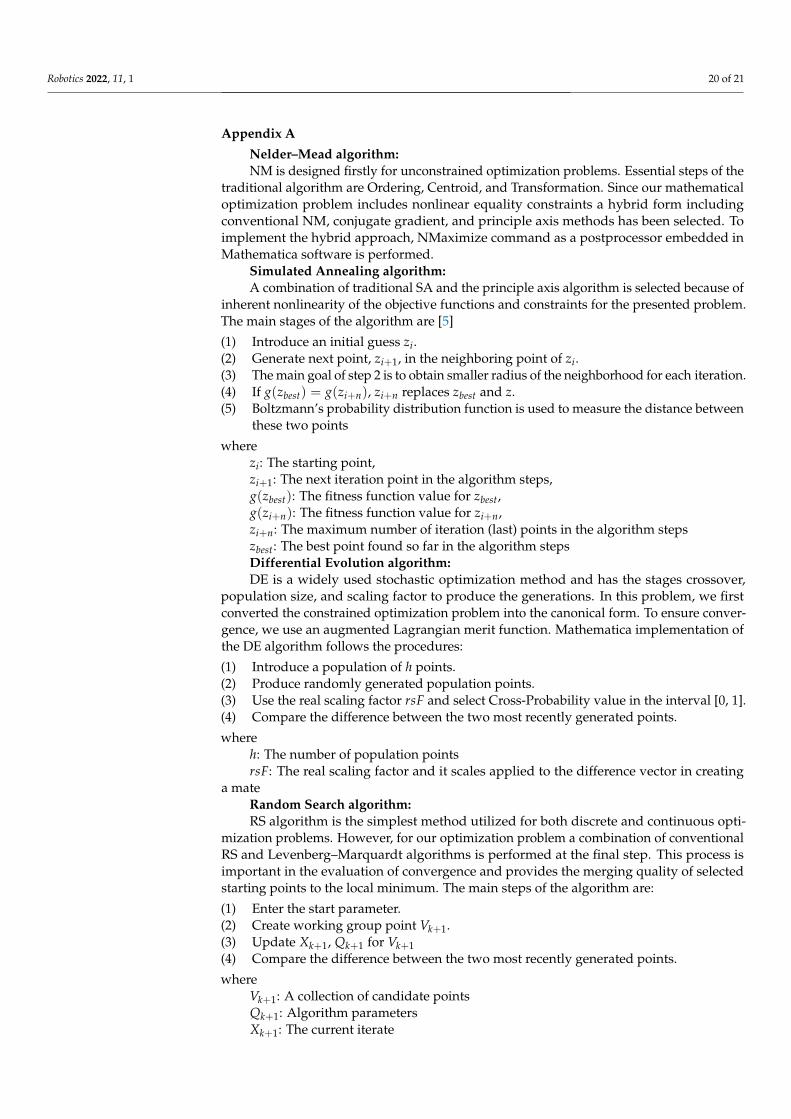
Robotics 2022, 11, 1 20 of 21

Appendix A

Nelder–Mead algorithm:NM is designed firstly for unconstrained optimization problems. Essential steps of the

traditional algorithm are Ordering, Centroid, and Transformation. Since our mathematicaloptimization problem includes nonlinear equality constraints a hybrid form includingconventional NM, conjugate gradient, and principle axis methods has been selected. Toimplement the hybrid approach, NMaximize command as a postprocessor embedded inMathematica software is performed.

Simulated Annealing algorithm:A combination of traditional SA and the principle axis algorithm is selected because of

inherent nonlinearity of the objective functions and constraints for the presented problem.The main stages of the algorithm are [5]

(1) Introduce an initial guess zi.(2) Generate next point, zi+1, in the neighboring point of zi.(3) The main goal of step 2 is to obtain smaller radius of the neighborhood for each iteration.(4) If g(zbest) = g(zi+n), zi+n replaces zbest and z.(5) Boltzmann’s probability distribution function is used to measure the distance between

these two points

wherezi: The starting point,zi+1: The next iteration point in the algorithm steps,g(zbest): The fitness function value for zbest,g(zi+n): The fitness function value for zi+n,zi+n: The maximum number of iteration (last) points in the algorithm stepszbest: The best point found so far in the algorithm stepsDifferential Evolution algorithm:DE is a widely used stochastic optimization method and has the stages crossover,

population size, and scaling factor to produce the generations. In this problem, we firstconverted the constrained optimization problem into the canonical form. To ensure conver-gence, we use an augmented Lagrangian merit function. Mathematica implementation ofthe DE algorithm follows the procedures:

(1) Introduce a population of h points.(2) Produce randomly generated population points.(3) Use the real scaling factor rsF and select Cross-Probability value in the interval [0, 1].(4) Compare the difference between the two most recently generated points.

whereh: The number of population pointsrsF: The real scaling factor and it scales applied to the difference vector in creating

a mateRandom Search algorithm:RS algorithm is the simplest method utilized for both discrete and continuous opti-

mization problems. However, for our optimization problem a combination of conventionalRS and Levenberg–Marquardt algorithms is performed at the final step. This process isimportant in the evaluation of convergence and provides the merging quality of selectedstarting points to the local minimum. The main steps of the algorithm are:

(1) Enter the start parameter.(2) Create working group point Vk+1.(3) Update Xk+1, Qk+1 for Vk+1(4) Compare the difference between the two most recently generated points.

whereVk+1: A collection of candidate pointsQk+1: Algorithm parametersXk+1: The current iterate

Robotics 2022, 11, 1 21 of 21

References1. Holland, J.H. Genetic Algorithms and the Optimal Allocation of Trials. SIAM J. Comput. 1973, 2, 88–105. [CrossRef]2. Colorni, A.; Dorigo, M.; Maniezzo, V. Distributed Optimization by Ant Colonies. In Toward a Practice of Autonomous Systems,

Proceedings of the First European Conference on Artificial Life, Paris, France, 11–13 December 1991; Varela, F.J., Bourgine, P., Eds.;Elsevier: Paris, France, 1992; pp. 134–142.

3. Kennedy, J.; Eberhart, R. Particle Swarm Optimization (PSO). In Proceedings of the IEEE International Conference on NeuralNetworks, Perth, Australia, 27 November–1 December 1995; pp. 1942–1948. [CrossRef]

4. Ab Wahab, M.N.; Nefti-Meziani, S.; Atyabi, A. A Comprehensive Review of Swarm Optimization Algorithms. PLoS ONE 2015,10, e0122827. [CrossRef]

5. Erten, H.I.; Deveci, H.A.; Artem, H.S. Stochastic Optimization Methods. In Designing Engineering Structures Using StochasticOptimization Methods; Aydin, L., Artem, H.S., Oterkus, S., Eds.; CRC Press: Boca Raton, FL, USA, 2020; pp. 10–23. [CrossRef]

6. Nakamura, Y. Advanced Robotics: Redundancy and Optimization, 1st ed.; Addison-Wesley Longman Publishing Co., Inc.: Boston,MA, USA, 1990.

7. Briot, S.; Goldsztejn, A. Topology Optimization of Industrial Robots: Application to a Five-Bar Mechanism. Mech. Mach. Theory2018, 120, 30–56. [CrossRef]

8. Vulliez, M.; Zeghloul, S.; Khatib, O. Design Strategy and Issues of the Delthaptic, a New 6-DOF Parallel Haptic Device. Mech.Mach. Theory 2018, 128, 395–411. [CrossRef]

9. Iqbal, H.; Aized, T. Workspace Analysis and Optimization of 4-Links of an 8-DOF Haptic Master Device. Rob. Auton. Syst. 2014,62, 1220–1227. [CrossRef]

10. Dede, M.I.C.; Kiper, G.; Ayav, T.; Özdemirel, B.; Tatlıcıoglu, E.; Hanalioglu, S.; Isıkay, I.; Berker, M. Human–Robot Interfaces ofthe NeuRoboScope: A Minimally Invasive Endoscopic Pituitary Tumor Surgery Robotic Assistance System. J. Med. Device 2021,15, 011106. [CrossRef]

11. De Luca, A.; Oriolo, G. The Reduced Gradient Method for Solving Redundancy in Robot Arms. In IFAC 11th Triennial WorldGongress; Elsevier: Tallinn, Estonia, 1990; Volume 23, pp. 133–138. [CrossRef]

12. Peng, Z.X.; Adachi, N. Compliant Motion Control of Kinematically Redundant Manipulators. IEEE Trans. Robot. Autom. 1993, 9,831–836. [CrossRef]

13. Seraji, H. Configuration Control of Redundant Manipulators: Theory and Implementation. IEEE Trans. Robot. Autom. 1989, 5,472–490. [CrossRef]

14. Nakamura, Y.; Hanafusa, H.; Yoshikawa, T. Task-Priority Based Redundancy Control of Robot Manipulators. Int. J. Rob. Res. 1987,6, 3–15. [CrossRef]

15. Uzunolu, E.; Tatliciolu, E.; Dede, M.C. A Multi-Priority Controller for Industrial Macro-Micro Manipulation. Robotica 2020, 39,217–232. [CrossRef]

16. Dede, M.I.C.; Maaroof, O.W.; Tatlicioglu, E. A New Objective Function for Obstacle Avoidance by Redundant Service Robot Arms.Int. J. Adv. Robot. Syst. 2016, 13, 48. [CrossRef]

17. Tatlicioglu, E.; Braganza, D.; Burg, T.C.; Dawson, D.M. Adaptive Control of Redundant Robot Manipulators with Sub-TaskObjectives. Robotica 2009, 27, 873–881. [CrossRef]

18. Maaroof, O.W.; Gezgin, E.; Dede, M.I.C. General Subtask Controller for Redundant Robot Manipulators. In Proceedings of the2012 12th International Conference on Control, Automation and Systems, Jeju, Korea, 17–21 October 2012; IEEE: Piscataway, NJ,USA, 2012; pp. 1352–1357.

19. Maaroof, O.W.; Dede, M.I.C. Physical Human-Robot Interaction: Increasing Safety by Robot Arm’s Posture Optimization. InProceedings of the ROMANSY 21—Robot Design, Dynamics and Control. ROMANSY21 2016. CISM International Centre forMechanical Sciences (Courses and Lectures), Udine, Italy, 20–23 June 2016; Parenti-Castelli, V., Schiehlen, W., Eds.; Springer:Cham, Switzerland, 2016; Volume 569, pp. 329–337. [CrossRef]

20. Yoshikawa, T. Manipulability and Redundancy Control of Robotic Mechanisms. In Proceedings of the IEEE InternationalConference on Robotics and Automation, St. Louis, MO, USA, 25–28 March 1985; IEEE: Piscataway, NJ, USA, 1985; pp. 1004–1009.[CrossRef]

21. Yoshikawa, T. Dynamic Manipulability of Robot Manipulators. Trans. Soc. Instrum. Control Eng. 1985, 21, 970–975. [CrossRef]22. Denavit, J.; Hartenberg, R.S. A Kinematic Notation for Lower Pair Mechanisms Based on Matrices. ASME J. Appl. Mech. 1955, 22,

215–221. [CrossRef]23. Paul, R.P.; Stevenson, C.N. Kinematics of Robot Wrists. Int. J. Rob. Res. 1983, 2, 31–38. [CrossRef]24. Salisbury, J.K.; Craig, J.J. Articulated Hands: Force Control and Kinematic Issues. Int. J. Rob. Res. 1982, 1, 4–17. [CrossRef]25. Chiu, S.L. Task Compatibility of Manipulator Postures. Int. J. Rob. Res. 1988, 7, 13–21. [CrossRef]26. Merlet, J.-P. Parallel Robots, 2nd ed.; Springer Science & Business Media: Berlin/Heidelberg, Germany, 2006.27. Asada, H. A Geometrical Representation of Manipulator Dynamics and Its Application to Arm Design. ASME. J. Dyn. Sys. Meas.

Control 1983, 105, 131–142. [CrossRef]28. Colgate, J.E.; Brown, J.M. Factors Affecting the Z-Width of a Haptic Display. In Proceedings of the IEEE International Conference

on Robotics and Automation, San Diego, CA, USA, 8–13 May 1994; IEEE: Piscataway, NJ, USA, 1994; pp. 3205–3210. [CrossRef]29. Yoshikawa, T. Foundations of Robotics: Analysis and Control; MIT Press: Cambridge, MA, USA, 1990.