Ecological Modelling 169 (2003) 131–155

A remote sensing-based primary production modelfor grassland biomes

J.W. Seaquista,∗, L. Olssonb, J. Ardöc

a Department of Geography& Centre for Climate and Global Change Research, McGill University,805 Sherbrooke St. W., Montreal, Quebec, Canada H3A 2K6

b Centre for Environmental Studies, Lund University, Box 170, S-221 00 Lund, Swedenc Department of Physical Geography and Ecosystems Analysis, Lund University, Box 118, S-221 00 Lund, Sweden

Received 13 February 2002; received in revised form 17 June 2003; accepted 16 July 2003

Abstract

That data from polar orbiting satellites have detected a widespread increase in photosynthetic activity over the last 20 yearsin the grasslands of the Sahel is justifies investigating its role in the tropical carbon cycle. But this task is undermined becauseground data that are generally used to support the use of primary production models elsewhere are lacking. In this paper, weprofile a Light Use Efficiency (LUE) model of primary production parameterised with satellite information, and test it for theWest African Sahel; solar radiation is absorbed by plants to provide energy for photosynthesis, while moisture shortfalls controlthe efficiency of light usage. In particular, we show how an economical use of existing, yet meagre data sets can be used tocircumvent nominal, yet untenable approaches for achieving this for the region. Specifically, we use a cloudiness layer providedwith the NOAA/NASA 8 km Pathfinder Land data archive (PAL) data set to derive solar radiation (and other energy balanceterms) required to implement the model (monthly time-step). Of particular note, we index growth efficiency via transpiration bysubsuming rangeland-yield formulations into our model. This is important for partially vegetated landscapes where the fate ofrainfall is controlled by relative vegetation cover. We accomplish this by using PAL-derived Normalised Difference VegetationIndex (NDVI) to partition the landscape into fractional vegetation cover. A bare soil evaporation model that feeds into bucketmodel is then applied, thereafter deriving actual transpiration (quasi-daily time-step). We forgo a formal validation of the modeldue to problems of spatial scale and data limitations. Instead, we generate maps showing model robustness via Monte Carlosimulation. The precision of our Gross Primary Production (GPP) estimates is acceptable, but falls off rapidly for the northernfringes of the Sahel. We also map the locations where errors in the driving variables are mostly responsible for the bulk ofuncertainty in predicted GPP, in this case the water stress factor and the NDVI. Comparisons with an independent model ofprimary production, CENTURY, are relatively poor, yet favourable comparisons are made with previous primary productionestimates found for the region in the literature. A spatially exhaustive evaluation of our GPP map is carried out by regressingrandomly sampled observations against integrated NDVI, a method traditionally used to quantify absolute amounts of primaryproduction. Our model can be used to quantify stocks and flows of carbon in grasslands over the recent historical period.© 2003 Elsevier B.V. All rights reserved.

Keywords:Light Use Efficiency; Gross Primary Production; Grasslands; NDVI; Sahel; Carbon cycle

∗ Corresponding author. Tel.:+1-514-398-4347;fax: +1-514-398-7437.

E-mail address:Jonathan.Seaquist@mcgill.ca (J.W. Seaquist).

1. Introduction

Net Primary Production (NPP) is an importantcomponent of the carbon cycle and a key indicator

0304-3800/$ – see front matter © 2003 Elsevier B.V. All rights reserved.doi:10.1016/S0304-3800(03)00267-9

132 J.W. Seaquist et al. / Ecological Modelling 169 (2003) 131–155

of ecosystem performance (Lobell et al., 2002). Fortracking the recent history of continental-scale veg-etation dynamics, the Normalised Difference Vege-tation Index (NDVI) derived from reflectance dataregistered by the ‘National Oceanic and AtmosphericAdministration’ Advanced Very High Resolution Ra-diometer (NOAA AVHRR) has traditionally beenused and regarded as a surrogate measure of primaryproduction (Box et al., 1989). However, recent workshows that this index is only a measure of photosyn-thetic potential (Runyon et al., 1994). Though theNDVI is a quantitative measure, it only yields esti-mates of relative vegetation amounts. The NDVI maybetter be used for parameterising models that maymore accurately reflect actual changes in primary pro-duction, as well as quantifying its absolute amount.Many sophisticated models of this type are now ap-plied routinely in North American and European con-texts for tracing the history of ecosystem dynamics,especially in the context of regional or global carbonbudgets (e.g.Ruimy et al., 1996; Veroustraete et al.,1996; Kimball et al., 1997; Goetz et al., 1999; Coopset al., 2001; Lobell et al., 2002; Reeves et al., 2001).But the ground-based data networks that most of thesemodels require to generate reliable estimates of pri-mary production at regional or continental scales arelacking for large parts of the Earth’s surface, gener-ally due to a dearth of infrastructure, economic woes,and a sparse population. One such region is the Sahelbelt of North Africa.Eklundh and Olsson (2003)flagthe Sahel as a hotspot for land cover change. For theperiod 1982–1999, they identify large areas of strongpositive trends in NDVI derived from data from theNOAA AVHRR. These findings suggest that the Sa-hel may play a significant role in the tropical carboncycle, and constitute at least part of the missing trop-ical carbon sink discussed bySchimel et al. (2001).From a humanitarian perspective, this region suffersfrom frequent drought and famine (Hulme, 1989;Olsson, 1993; Nicholson et al., 1998), both of whichare intimately tied to primary production.

2. Objectives

This paper describes and tests a satellite data-drivenLight Use Efficiency (LUE) model for mapping pri-mary production and tracing its dynamics over the re-

cent historical period (20 years) for the case of theWest African Sahel. Another objective is to assessmodel performance using Monte Carlo simulations,comparisons with other models, and previous resultsfor the region reported in the literature.

3. The LUE concept with emphasis on previousapplications in the Sahel

3.1. LUE concept

NPP represents the net flow of carbon to plantsfrom the atmosphere and defines a balance betweengross photosynthesis (GPP—Gross Primary Produc-tion) and autotrophic respiration. GPP defines photo-synthesis before autotrophic respiration losses, whileNet Ecosystem Production is NPP less heterotrophicrespiration (Maisongrande et al., 1995; Field et al.,1995; Gower et al., 1999).

The remote sensing-based LUE model is defined asfollows, and has evolved fromMonteith (1972, 1977):

GPP=n∑i=1

εpε(aNDVI + b)PAR (1)

where GPP is the Gross Primary Production summedover the growing season (g m−2), εp is the maximumbiological efficiency of PAR conversion to dry mat-ter (g MJ−1 m−2), ε is the environmental stress scalar,NDVI is the (NIR − RED)/(NIR + RED) (unitless),PAR is the incoming photosynthetically active radia-tion (MJ m−2), anda andb are the regression coeffi-cients.

The NIR and RED refer to unitless reflectances inthe near infrared and red portions of the electromag-netic spectrum as measured by the AVHRR sensormounted on the series of NOAA satellites. The NDVIhas often been used as a surrogate measure of primaryproduction (Box et al., 1989), yet recent findings sug-gest that the NDVI is unsatisfactory for this purposedue to the uncoupling of PAR absorption and plantgrowth (Runyon et al., 1994). In contrast to the earlierempirical models that related growing season sumsof NDVI to geo-referenced samples of above-groundNPP (e.g.Tucker et al., 1985; Prince, 1991a), this ap-proach boasts axiomatic rigour (Prince, 1991b) andhas the potential to estimate biomass in absolute terms

J.W. Seaquist et al. / Ecological Modelling 169 (2003) 131–155 133

across different climatic regimes, site characteristics,and scales, thus eliminating the demand for frequentcalibration (Reeves et al., 2001).

PAR encompasses the domain of incoming solarradiation between 0.4 and 0.7�m, and allows greenvegetation to undergo photosynthesis (Hall and Rao,1994). It varies as a function of solar zenith an-gle, cloudiness and the concentration of atmosphericconstituents (water vapour and aerosols), but overtime-scales of 1 day or longer, its contribution toincoming global radiation fluctuates within a nar-row range between 45 and 50% (Frouin and Pinker,1995). Fraction of Photosynthetically Active Radi-ation (FPAR) denotes the fraction of incident PARabsorbed by plants that is used for photosynthesisand is represented here in terms of NDVI. Sensitivitystudies with radiation transfer models indicate therelationship remains robust in the presence of pixelheterogeneity, vegetation clumping, and variationsin leaf orientation and optical properties (Gowardand Huemmrich, 1992; Begue, 1993; Myneni andWilliams, 1994). Good area averages may also beprovided given the scale invariance of the relation-ship. This is the pivotal link that facilitates broad scaleprimary production mapping using the NDVI from theNOAA AVHRR sensor, since it provides a measureof photosynthetic potential (Goetz and Prince, 1999).

The biological efficiency term has been the fo-cus of much debate. Ambiguity and confusion havearisen because this parameter has been determinedusing inconsistent methods; it sometimes correspondsto total NPP, and often to above-ground NPP, butrarely to GPP (Gower et al., 1999). It also differsbetween C3 and C4 plants. Sometimes it has beendeduced from measurements of global radiation orat other times, the PAR intercepted by a vegetationcanopy, instead of APAR (e.g.Gower et al., 1999).Some remotely-sensed based models resort to usinga theoretical maximum value,εp, predicated on thequantum yield and CO2-dry-matter-conversion factor,multiplied by stress scalars,ε, that yield GPP afterwhich respiration terms are assessed (e.g.Prince andGoward, 1995; Goetz et al., 1999). Still others deter-mine a bulk efficiency term (εpε from Eq. (1)) fromthe slope of daily integrated CO2 versus PAR re-gressions (e.g.Maisongrande et al., 1995), thereafteraccounting for respiration terms. Finally, ecophysi-ological simulation models with non-trivial assump-

tions regarding plant growth and environment may beused to derive this bulk efficiency term after which re-motely sensed data are pulled in to compute primaryproduction (White and Running, 1994; Mougin et al.,1995; Handcock, 2001). Stress factors (lumped asεin Eq. (1)) that down-regulate the potential growthefficiency,εp, may include drought, temperature ex-tremes, pollution, herbivory, insufficient nutrients, dis-ease, etc. (Prince, 1991b) and can vary on timescalesfrom seconds to months. Theoretically derived po-tential efficiencies range between 1.1 and 8.4 g MJ−1,while plot studies of bulk efficiencies give ranges be-tween 0.42 and 3.8 g MJ−1 (Goetz and Prince, 1999).

3.2. Previous applications of the LUE approachin the Sahel

Early applications of the satellite-based LUEmodel in the Sahel prescribed bulk biological ef-ficiency values from the literature (either a singlevalue, or vegetation-specific values) to estimate arealabove-ground NPP or crop yield using remotelysensed data with seemingly acceptable results (e.g.Bartholome, 1990; Cherchali et al., 1995). However,given the considerable heterogeneity of the Sahelianlandscape in terms of resource availability, doubt hadbeen cast on an invariant bulk biological efficiencyterm, even for a given species (Begue et al., 1991;Prince, 1991b; Guerif et al., 1993; Hanan et al.,1995). Rasmussen (1998)tested and rejected the hy-pothesis of stable bulk biological growth efficiencyfor the Senegalese Sahel and elucidated some of thefundamental relations between above-ground NPP,NOAA AVHRR NDVI imagery, and the environment,by showing that residual unexplained variance in em-pirical NDVI–NPP relations could be reduced by in-cluding surface temperature and percent tree cover inmultivariate regression models. Though it is now ev-ident that the bulk biological growth efficiency is notconstant, it may converge on a narrow range of valuesfor particular plant functional types in terms of GPP,but not NPP, due to differences in respiration costs.The underlying tenet of the functional convergencehypothesis maintains that plants have been tunedthrough natural selection to maximise photosyntheticgain per unit APAR (GPP) by optimising resourceallocation in environments with limited resources andhigh acquisition costs (Goetz and Prince, 1999). This

134 J.W. Seaquist et al. / Ecological Modelling 169 (2003) 131–155

is the major appeal of the LUE approach for computingGPP using remote sensing (Goetz and Prince, 1999).

4. Test area—West African Sahel

The area covers most of Niger and parts of Mali,Burkina Faso, Benin, Nigeria, the Congo, and Chad(between 11◦N and 20◦N and 1◦W and 18◦E) all ofwhich are located in the ‘Continental Sahel’, a term de-fined by its recognition as a homogeneous rainfall re-gion (Agnew and Chappell, 1999) (Fig. 1). The climateranges from arid to semi-arid with a sharp north-southprecipitation gradient (Maselli et al., 1992). Mean an-nual rainfall totals range from less than 100 mm year−1

in the north to almost 1000 mm in the south. An-nual evapotranspiration far exceeds annual rainfall andranges from 1800 to 2300 mm (Le Houerou, 1980;Rockström, 1997). The rains begin with the north-ward migration of the inter-tropical convergence zonein May and subside with its southward retreat aroundthe beginning of October. The north is sparsely vege-tated with bush-land dominating, giving way to grass-land, savannah, and woody savannah in the far south.The vegetation is adapted to a warm, dry climate, withmost grasses using the C4 photosynthetic pathway,while woody species and some herbs exhibit the C3

Fig. 1. Map of study area showing International Geosphere Biosphere land cover classes.

(Le Houerou et al., 1993). Marked annual fluctuationsoccur in the proportion of the different grass speciesgrowing at any one site. Nomadic pastoralism is thedominant land use in the north, giving way to shiftingor fallow cultivation rotation in the south. Major cropsgrown include millet, maize sorghum, and cowpea, allof which are C4 species (Le Houerou, 1980). The soilsare sandy with low organic and nutrient content, whiletopographical variations are generally less than 500 mwithin the vegetated zones (Le Houerou, 1980).

5. Data sources and preparation

5.1. NOAA/NASA Pathfinder Land data set

We used daily data from the NOAA/NASAPathfinder Land data archive (PAL) data set to derivemany of the parameters needed forEq. (1). The PALhas spatial resolution of 8 km and includes layersfor solar zenith angle, satellite look and azimuth an-gles, cloud and quality flags, as well as the originalfive channels of the NOAA AVHRR sensor (red andnear-infrared reflectance, and three thermal) (Table 1).These data come corrected for Rayleigh scatteringand ozone absorption, and include post-flight sensorcalibration (James and Kalluri, 1994; Smith et al.,

J.W. Seaquist et al. / Ecological Modelling 169 (2003) 131–155 135

Table 1Data layers provided with the PAL data set

Parameter Units Field width Offset Gain

NDVI – 8 128 0.008CLAVR – 8 1 1Quality control flag – 8 1 1Scan angle Radians 16 10481.98 0.0001Solar zenith angle Radians 16 10 0.0001Relative azimuth angle Radians 16 10 0.0001Channel 1 reflectance % 16 10 0.002Channel 2 reflectance % 16 10 0.002Channel 3 brightness temperature Kelvin 16 −31990 0.005Channel 4 brightness temperature Kelvin 16 −31990 0.005Channel 5 brightness temperature Kelvin 16 −31990 0.005Julian day DDD·HH 16 10 0.01

1997a,b), and is the longest, most consistently pro-cessed global satellite imagery archive to date. Knownproblems include (1) under-estimation of the correc-tions for Rayleigh and ozone absorption; (2) red andnear-infrared channels were not normalised for solarzenith angle, and (3) incorrect computation of the solarzenith angle.Smith et al. (1997a,b)reported these er-rors affect the NDVI by at most 0.02 NDVI units. Thereason for choosing 1992 is the existence of a data setgenerated by theHAPEX-Sahel(Hydrologic Atmo-spheric Pilot Experiment in the Sahel—carried out insouthwest Niger in 1992) to aid in the construction ofour model. The main goal of this international projectwas to elucidate the mechanisms of land-atmospherefeedback at the scale of a grid cell for a generalcirculation model (1◦ × 1◦) (Prince et al., 1995).

Maximum value compositing is commonly em-ployed to mitigate unwanted atmospheric and viewangle effects in daily NDVI images by ‘collapsing’them into mosaics composed of the highest NDVIfor each location over a pre-specified time period bysequentially comparing pixels (Holben, 1986). Dueto the shortcomings of this method (e.g. Cihlar et al.,1994), we used an alternative approach that selectsonly those pixels with favourable viewing geometryand minimises bias (Seaquist, 2001). We then filteredthen NDVI time profiles using a modified best indexslope extraction method (Viovy et al., 1992; Lind andFensholt, 1999) to rid the images of residual cloudcontamination. Finally, we corrected them for the in-fluence of background soil reflectance afterLind andFensholt (1999).

5.2. Climate data

The climate data were used to derive both energybalance and soil moisture estimates used to computeε in Eq. (1). We incorporated climate data from fourdifferent sources. Mean monthly temperature andmonthly rainfall totals were merged from version 1.2of the Global Historical Climatology Network (Voseet al., 1992) data-base and the Climate Research Unitdata-base over the West African Sahel from between10◦N and 20◦N to 18◦W and 23◦E. Both these datasets have undergone extensive screening. The numberof rainfall stations for the period May–October wasboosted considerably by amalgamating them with1992 data fromAfrica Data Dissemination Service.Finally, a minimum and maximum of 79 rainfall sta-tions in November and 257 in June, respectively, wereretained (for temperature, 32 in January and 58 inOctober, respectively). Daily rainfall, and maximumand minimum temperature records for 16 synopticclimate stations across Niger for a 7-year period wereprovided by the National Meteorological Service inNiamey, Niger.

We generated total monthly rainfall surfaces forJune through September of 1992 with universal‘block’ kriging (see Matheron, 1971; Goovaerts,1997; Chappell et al., 2001for more detailed dis-cussions of this technique) in order to scale up orestimates to match the spatial resolution of the satel-lite data. Accuracies derived from cross-validation ofthese variogram models varied between 15 and 20%from June to September. We used thin plate splines

136 J.W. Seaquist et al. / Ecological Modelling 169 (2003) 131–155

to interpolate rainfall for other months given that (1)there were fewer stations recording rainfall, (2) uni-versal kriging techniques were deemed inappropriateafter checking the rainfall distributions (which werehighly skewed), and (3) most photosynthesis occursduring the rainy season.

Monthly mean temperatures exhibited smooth andrestricted variation. Since there were too few stationsto interpolate reliably with kriging, we interpolatedusing thin plate splines (yielding an root mean squareerror of 0.7◦C, obtained by leaving HAPEX-Saheltemperature data out of the interpolation procedure).

5.3. Land cover

The Africa Land Cover Characteristics Data-Baseversion 1.2 with the International Geosphere Bio-sphere Programme legend provided us with informa-tion on land cover (USGS, 2000). This data layer wasnot used explicitly in our model, but rather to guideour analyses and the interpretation of our results. Thedata-base was generated at a 1-km spatial resolution,and was derived from AVHRR data acquired betweenApril 1992 and March 1993. The spatial resolutionwas degraded to 8 km to ensure compatibility with thePAL data set (Fig. 1). The land cover classificationhas an overall accuracy of 83%, though accuracy wassomewhat reduced for the Sahel, with 67% for bothshrub-land and savannah (Loveland et al., 1999).

5.4. FAO digital soil map of the world

Since we required information on water holding ca-pacity for the computation of our water stress factor,ε (Eq. (1)), we took the maximum soil moisture stor-age, computed from topsoil texture and soil depth,from version 3.5 of the Food and Agriculture Organi-zation (FAO) Digital Soil Map of the World (1995) atscale of 1:5,000,000. We recoded the map to obtainestimates of soil moisture storage capacity to an im-permeable layer, or to a depth of 100 cm, by takingthe centres of the ranges provided in their data-base.For contiguous regions showing a combination of twocategories, we applied weighted averaging. The FAOstates that the estimation of maximum soil moisturestorage was determined in isolation of the prevailingclimate and largely ignores the rooting behaviour ofvegetation and that the reliability of the soil type clas-

sification is questionable for some regions of Africa.This data layer is the only source of information avail-able at this scale.

6. Methods

Fig. 2 illustrates the processing stream. The param-eters inside the ellipsoids represent the raw data (in-cluding constants derived from the literature) used inthe model, whereas the parameters inside the boxes arederived during the execution of the model. Note thatEq. (1) is a highly generalised form of this flowchart,and is depicted in the shaded boxes inFig. 2. Themethods described below are to be reviewed with di-rect reference toEq. (1)andFig. 2.

6.1. PAR

We estimated PAR on cell-by-cell basis to an ac-ceptable level of accuracy (root mean square errorof 35.4 MJ m−2 month−1) for use with a terrestrialLUE model using the daily CLAVR (CLouds fromAVHRR) layer from the PAL data set in combinationwith Ångström’sequation (Fig. 3a). ThoughSeaquistand Olsson (1999)demonstrate the methodology indetail, we outline the rudiments of this calculation inAppendix A.

6.2. FPAR and APAR

We linearly scaled FPAR between the lower andupper limits of bare soil and maximum NDVI,respectively (NDVI = 0.04, for 0% absorption,and NDVI = 0.61, 95% absorption) (Goward andHuemmrich, 1992; Potter et al., 1993; Guerif et al.,1993; Ruimy et al., 1996; Prince et al., 1995; Hananet al., 1995; Goetz et al., 1999; Lind and Fensholt,1999; Handcock, 2001):

FPAR= 1.67(NDVI )− 0.07 (2)

Note thatEq. (2)is the term inside the parentheses inEq. (1). An NDVI value of 0.04 was determined forbare soil by taking its mean during the dry season,while 0.61 corresponds to a growing season NDVIalong the shore of Lake Chad where vegetation is verydense. Finally, we merged the images into monthlymeans to further reduce noise (Eklundh, 1996;

J.W. Seaquist et al. / Ecological Modelling 169 (2003) 131–155 137

Fig. 2. Flowchart of LUE model.

Kaisischke and French, 1997) thereafter computingAPAR as the product of PAR and FPAR for eachmonth (Fig. 3b).

6.3. Potential biological growth efficiency—εp

We assigned a value of 5 g MJ−1 for εp (the poten-tial biological efficiency), which indicates a mixtureof C3 and C4 plants with the assumption that for thegreater part of a growing season, C4 grasses dominatethe NOAA AVHRR reflectance signal. Typical Sahe-lian rangeland consists of a mixture of both C3 and C4plants, with C3 forbs dominating early in the growingseason, giving way to C4 grasses later in the growingseason (Hanan et al., 1995, 1997), at least for typicalsites in the HAPEX-Sahel and in the Gourma regionof Mali. Mougin et al. (1995)found the C3/C4 ratio tobe 43/57 for Mali’s Ferlo district. The Global Produc-tion Efficiency Model ofPrince and Goward (1995)and Goetz et al. (1999)uses a value of 6.1 g MJ−1

for C4 plants (invariant with temperature), while theymodel C3 values based on leaf biochemical processes.The potential efficiency of C3 plants is generallylower, especially for the higher temperatures of Sa-helian environments. Without regardingPrince andGoward’s (1995)C3 potential efficiency sub-routine,all other models, irrespective of complexity, resortto prescribing these values, or conduct error minimi-sation exercises with actual biomass measurementsor use regressions of PAR against CO2 fluxes (e.g.Potter et al., 1993; Mougin et al., 1995; Ruimy et al.,1996).

6.4. Water stress scalar—ε

Water is generally assumed is the primary factorlimiting photosynthesis in the region at these scales(Le Houerou, 1980; Verstraete and Pinty, 1991). Wetherefore reformulated the equations inWight andHanks (1981)andMillington et al. (1994), replacing

138 J.W. Seaquist et al. / Ecological Modelling 169 (2003) 131–155

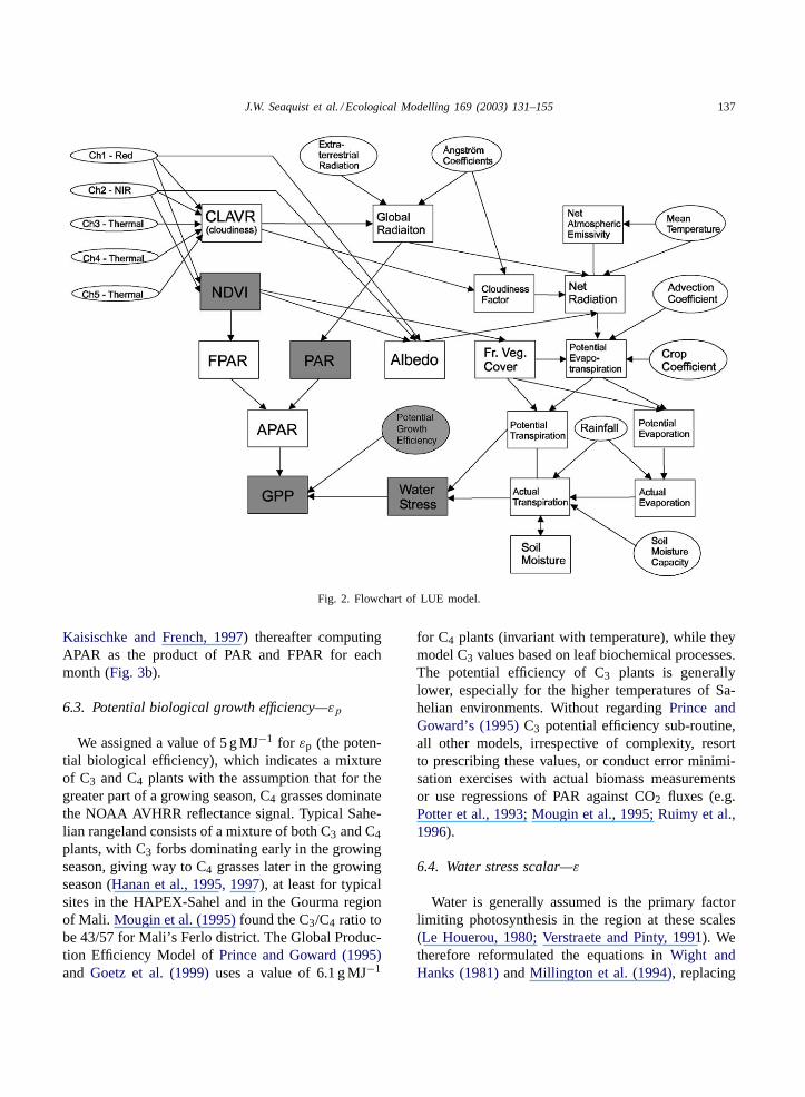
Fig. 3. (a) Total photosynthetically active radiation for the growing season (May–October). (b) Total photosynthetically active radiationabsorbed by plant canopy for the growing season. (c) Total potential evapotranspiration for the growing season. (d) Total actual evapotran-spiration for the growing season.

their crop yield terms with GPP

GPPa

GPPp= Ta

Tp(3)

where GPPa is the Gross Primary Production (g m−2),GPPp is the potential Gross Primary Production(g m−2), Ta is the actual transpiration (mm), andTpis the potential transpiration.

The ratio of actual transpiration to potential tran-spiration is the water stress scalar. Note that in termsof Eq. (1), GPPp is directly analogous to the productof the growing season sum of APAR and the potentialbiological efficiency,εp. The purpose ofEq. (3) is toprovide a logical argument and point of departure forour derivation of water stress,ε. The calculation ofpotential transpiration is discussed first, followed byactual transpiration.

A realistic assessment of actual transpiration (aswell as actual evapotranspiration) from partiallyvegetated surfaces requires, as a minimum, the sep-arate treatment of bare soil and plant components(Hanks, 1974; Wight and Hanks, 1981; Wallace et al.,1993; Millington et al., 1994; Mougin et al., 1995;Srivastava et al., 1997). We therefore partitioned our

estimate of potential evapotranspiration (see deriva-tion below) into bare soil and vegetation componentsby transforming the NDVI into fraction of vegetationcover ranging from 0 (no vegetation cover) and 1 (fullvegetation cover). We followedChoudhury (1994),Capehart (1996), andCarlson and Ripley (1997):

Ep = KcETp

[1 −

(NDVI − NDVIo

NDVIs − NDVIo

)2]

(4)

Tp = KcETp

(NDVI − NDVIo

NDVIs − NDVIo

)2

(5)

whereEp is the bare soil potential evaporation (mm),Tp is the potential transpiration (mm),Kc is the cropcoefficient, ETp is the potential evapotranspiration(mm), NDVI is the cell-specific NDVI, NDVIs is theNDVI corresponding to full vegetation cover (0.50),and NDVIo is the bare soil NDVI (0.04).

The logic behindEqs. (4) and (5)are outlined inAppendix B. We assigned a constant value of 0.85in accordance with typical mean growing seasonvalues for rangeland vegetation (Wight and Hanks,1981; Millington et al., 1994). We used thePriestleyand Taylor (1972)method for computing potential

J.W. Seaquist et al. / Ecological Modelling 169 (2003) 131–155 139

evapotranspiration (Fig. 3c) for Eqs. (4) and (5)be-cause of its direct physical link with radiation, itssuccess in operational agro-meteorological monitor-ing, data availability, as well as its suitability for largeareas (Bastiaanssen, 1995; Jiang and Islam, 1999):

ETp = αa∆

∆+ γ(Rn −G) (6)

whereαa is the advection parameter,∆ is the gradientof saturated vapour pressure (kPa◦C−1), γ is the psy-chrometric constant (kPa◦C−1), Rn is the net radiation(MJ m−2), andG is the ground heat flux (MJ m−2).

The ground heat flux is considered negligible andis ignored. Most measurements in humid, temperateenvironments have shown that the advection parame-ter takes on a conservative value of about 1.3, thoughin arid environments, values in excess of 1.75 arereported (Jensen et al., 1990), likely due to the en-trainment of heat from both above and below, leadingto a significant increase in the depth of the plane-tary boundary layer (Monteith and Unsworth, 1990;L’homme, 1996). We selected a value of 1.46 (basedon monthly sums) as this number optimised theagreement between estimated and measured potentialevapotranspiration giving an root mean square error of16.3 mm against ground data from the HAPEX-Sahelexperimental site at a monthly time step.Appendix Coutlines the computation of net radiation inEq. (6).

We then calculated the actual transpiration (seeEq. (3)) with a simple bucket model where the rootzone is given as a single layer with a constant waterholding capacity where:

Ta(t) = SM(t) + R(t) − Ea(t) − SM(t+1) −D(t) (7)

wheret is the day, SM is the soil moisture (mm),Ris the rainfall (mm),Ea is the actual evaporation frombare soil (mm),T is the transpiration (mm),D is thedrainage and runoff (mm).

The derivation of bare soil actual evaporation fromEq. (7)is given inAppendix D. Deep drainage, runoff,and run-on, are usually infrequent in semi-arid envi-ronments (Le Houerou, 1980; Lo Seen Chong et al.,1993; Mougin et al., 1995; Wythers et al., 1999) thesewere ignored. Water discharge in the Niger River con-firms the miniscule contribution of drainage and runoff(Nicholson et al., 1996). The primary function of thebucket model is to parameterise the effect of low soilmoisture on the stomatal conductance of vegetation,

giving a measure of the impact of drought stress onplant growth:

Ta = Tp, ifSM

SMmax≥ C (8)

Ta = Tp

C

SM

SMmax, if

SM

SMmax< C (9)

Ta is the actual transpiration (mm),Tp is the potentialtranspiration (mm), SM is same as defined previously,SMmax is the maximum soil water holding capacity(mm), andC is the critical fraction of available waterbelow which soil water deficit affects transpiration.

In reality, theC parameter varies with vegetationand crop type, and can range between 0.28 and 0.7(Wight and Hanks, 1981; Choudhury and DiGirolamo,1998). However, bothWight and Hanks (1981)andMillington et al. (1994)used a value of unity (lin-ear relationship) justified on (1) model insensitivityto values below 0.4, (2) the satisfactory performancefor rangeland vegetation in both North America andTunisia, and (3) the lack of information about thesedata. We assigned a value of 1. We spun up the bucketmodel by duplicating all pseudo-daily data for 1992four times (for a time-series of 4 years) to ensure thatour estimates achieved independence from arbitrarilyassigned initial soil moisture content.

Fig. 3d shows total growing season actual evap-otranspiration over the region. Our experiments thattested the sensitivity of actual evapotranspirationto ±20% variations in selected model soil textureparameters (seeAppendix D) as well as potentialevapotranspiration (corresponding to an area locatedin the East Central Supersite of the HAPEX-Sahel)revealed that it was most sensitive to rainfall. Ob-served actual evapotranspiration over a millet field(13◦33′N and 2◦39′E) in August, and over a herb site(13◦33′N and 2◦41′E) in both August and Septemberin the South Central Supersite of the HAPEX-Sahelnevertheless confirmed the realistic performance ofthe model (with the tendency to slightly overestimateactual evapotranspiration).

7. Results

Fig. 4ashows the final map of total growing seasonGPP (May–October). GPP is very low in the northern

140 J.W. Seaquist et al. / Ecological Modelling 169 (2003) 131–155

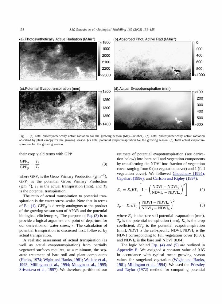
Fig. 4. (a) Growing season GPP for 1992. (b) Standard deviation expressed as a percentage of 1992 growing season GPP as calculatedfrom a Monte Carlo simulation; number of runs= 1000.

regions where it is too dry to support extensive plantcommunities. Local vegetation pockets are apparentin the mountains north of Agadez where elevations inare in excess of 2000 m. Other patches of GPP are as-sumed to occur around wadis. In these regions, GPP isgenerally less than 100 g m−2, though locally, this mayexceed 400 g m−2. The region of contiguous GPP be-gins just north of Lake Chad in the east and roughly ex-tends in a line north-westward to the middle part of thearea, before retreating south-westward. The northerlyportion of this belt is the pastoral zone supporting fod-

der for herds of domesticated sheep, goats and cattleduring the rainy season. GPP values here are generallybetween 100 and 500 g m−2. This roughly correspondsto ‘Grassland’ inFig. 1. Immediately to the south ofthis belt is found the mixed Cropland-vegetation Mo-saic where fields of millet and sorghum (with othercrops) are interspersed with fallow, containing indige-nous grassland and savannah species. GPP here rangesfrom between 500 and 1500 g m−2. Further south, GPPin excess of 1500 g m−2 shows the lush vegetationcommunities of the savannah and woody savannah

J.W. Seaquist et al. / Ecological Modelling 169 (2003) 131–155 141

Table 2Amount and proportion of primary production per land cover class

Land cover % Area GPP (Tg) % GPPtotal GPPmean

(g m−2)GPPstd NPPmean

(g m−2)Above-groundNPPmean (g m−2)

Barren/sparse 43.9 15.9 1.7 19.5 123.5 9.4 3.7Shrubland 13.1 9.0 1.0 37.1 69.2 17.8 7.1Grassland 18.3 120.1 13.1 352.8 298.2 169.3 67.7Savannah 17.8 578.4 62.9 1752.7 733.2 841.3 336.5Cropland-vegetation 6.3 185.8 20.1 1596.5 382.5 766.3 306.5Cropland 0.3 4.5 0.5 920.9 817.6 442.0 176.8Woody savannah 0.1 6.2 0.7 2831.8 490.5 1359.3 543.7Water 0.2 0.0 0.0 0.0 0.0 0.0 0.0

Summary 100.0 919.9 100.0 497.2 796.7 238.7 90.6

zones. Highest GPP is found around the northeastshores of Lake Chad (in excess of 3500 g m−2) wherethe high water table supports rich thickets of riparianvegetation.

We disaggregated our GPP estimates on the basisof land cover class (Table 2). Class totals of GPP aregiven, as well as their means per category, as wellas their standard deviations. Despite the spatial extentof the Barren/Sparsely vegetated category (compris-ing 42.9% of the total area), it supports less than 2%of the region’s GPP. Conversely, the savannah classcovers only 17.6% of the area, yet supports 63% ofthe region’s photosynthetic gain.

8. Evaluation

We used four techniques to assess model perfor-mance: (1) Monte Carlo simulations, (2) comparisonwith the results of a CENTURY model run, (3) qual-itative comparisons with other studies conducted inthe West African Sahel, and (4) evaluation against theclassical integrated NDVI approach for mapping pri-mary production. Direct comparison with ground es-timates of NPP were impossible partly due to lack ofdata, as well as the difficulties in reconciling the differ-ences in spatial resolution between our results (8 km)and ground samples (typically representative of a fewmetres at most).

8.1. Monte Carlo simulations

Monte Carlo simulation is a powerful and flexibleerror propagation technique. The driving parameters

of a model are varied randomlyN times accordingto their probability distributions. Each realisation isstored and then used to compute a mean and variancefor each cell (e.g.Burrough and McDonnell, 1998;Heuvelink, 1998; Crosetto et al., 2001). In the contextof Eq. (1), we define the following:

GPPu = 1

N

N∑i=1

GPPi (10)

GPPs2u = 1

N − 1

N∑i=1

(GPPi − GPPu)2 (11)

whereGPPu is the mean GPP computed fromu modelparameters,N is the number of simulations, GPPi is thesimulation-specific (i) GPP, GPPs2u is the GPP variancecomputed fromu model parameters.

We perturbed the parameters ofEq. (1)as inTable 3for N = 1000 runs per variable. All errors exceptthe NDVI are assumed to be stationary, and originatefrom normal distributions. We deliberately restrictedour Monte Carlo simulations to four lumped input pa-rameters due to the technique’s heavy computationaldemands.

Table 3Errors used for the Monte Carlo simulations

Inputparameter

Root mean squareerror

Determinationof error

Rank

NDVImin 0.01 (unitless) Literature 3NDVImax 0.05 (unitless) Literature 3PAR 35.0 (MJ m−2 month−1) Ground

measurements4

ε 0.2 (unitless) ‘Expert opinion’ 1εp g MJ m−2 month−1 Literature 2

142 J.W. Seaquist et al. / Ecological Modelling 169 (2003) 131–155

We established NDVI uncertainty fromKaufmanand Tanre (1996)who randomly select actual aerosoland water vapour optical thickness observations fromthe Senegalese Sahel (Soufflet et al., 1991) to simu-late top-of-the-atmosphere NDVI over a time-invariantground cover of fescue grass, assuming randomly dis-tributed cloud covers of 50%. Compositing for 9- and27-day periods yielded NDVI values of 0.61± 0.046and 0.65±0.027, respectively. The variations about themean result from residual atmospheric contamination,cloud, and scan angle effects. Since the compositingperiod used in this study is about 14 days, we chosea value of±0.05 to represent the uncertainty aroundthe maximum NDVI (0.61). We set bare soil NDVIuncertainty at±0.01 (0.04). The absolute value of theNDVI is not of primary interest here; rather, we wereinterested in the stability of the anchor points defin-ing the FPAR–NDVI relation. Quantisation artefactsmay potentially contribute precision uncertainties ofsimilar magnitude (depending on target brightness andsolar zenith angle), so our uncertainty estimates rep-resent a ‘best-case’ scenario. The primary impact ofvarying the NDVI is to alter thea andb parametersin the FPAR–NDVI relation (Eq. (2)), which is effec-tively equal to incorrectly identifying the NDVI valuesthat correspond to 95 and 0% PAR absorption. We de-termined the root mean square error for PAR directlyfrom Seaquist and Olsson (1999), briefly reviewed inAppendix A. We found it impossible to quantitativelydetermine a root mean square error for the water stressterm (ε) due to lack of data. We expect error contri-butions from the simplified assumptions used for therainfall and hydrology as well as the inaccuracies inmaximum soil water holding capacity, SMmax, andtherefore set it to±0.2 (unitless). Finally, we assumederror for the potential biological efficiency,εp, to be±1.0 g MJ−1. We determined this from the literaturewhile keeping in mind that the vegetation consists ofa blend of C3 and C4 species in geographically vary-ing proportions. The influence of mineral nutrition re-mained unknown.

The results are presented inFig. 4b. As a generalrule, the higher the GPP the more robust the predic-tion; standard deviations are less than 20% of totalGPP up to GPP values of about 1000 g m−2. Standarddeviations inflate to between 25 and 99% of GPP forthe southern and northern portions of the grasslandland cover class, respectively. We decomposed the to-

tal error variance into the proportion of error variancecontributed per model parameter (Fig. 5a–d). The PARterm lends the least error, generally less than 15%and decreases moving northward. The NDVI is rela-tively unimportant for determining the GPP of savan-nah and Cropland-vegetation Mosaic, but contributesover 90% of the total error variance in the northernportions of the grassland class. The potential biolog-ical growth efficiency,εp, rarely exceeds 30% of thetotal error variance, while the model is most sensitiveto the water stress scalar,ε.

8.2. The CENTURY model

The Monte Carlo simulation technique cannotreport bias. Independent estimates of primary pro-duction may be obtained from other models, suchas CENTURY. CENTURY is a ‘lumped parameter’,ecosystem model that can simulate biogeochemicalfluxes of carbon, nitrogen, phosphorous, and sulphur,as well as primary production and water balance ata monthly time step (Parton et al., 1987, 1988; Coleet al., 1989; Metherell et al., 1993). The driving vari-ables are monthly precipitation and monthly averageminimum and maximum temperature. Soil texture,litter nitrogen, lignin content, and tillage disturbanceare also important soil process rate controls. Themodel has been widely used and validated (Burkeet al., 1989; Parton et al., 1993, 1994, 1996; Bromberget al., 1996; Smith et al., 1997a,b; Mikhailova et al.,2000). The effects of fire, fertilisation, irrigation,grazing, various cultivation and harvest methods, etc.are possible to incorporate in the simulations.

We prescribed land cover type fromFig. 1 whichwe also used to determine land management charac-teristics (including fire frequencies, grazing character-istics, and fallow periods) for 16 sites across Niger(Fig. 6a) where data were available to run the model.Table 4shows the scenarios for the different land coverclasses. We derived soil texture from the Soil Mapof the World (FAO/UNESCO, 1995). Initial amountsof soil carbon and nitrogen were established by run-ning the model to equilibrium using long-term cli-mate averages. Only 7 years of climate data wereavailable for each station, so 3 years were randomlychosen and duplicated to bring the total up to 10years, the minimum amount of time necessary to gen-erate long-term climate estimates. No nitrogen fixation

J.W. Seaquist et al. / Ecological Modelling 169 (2003) 131–155 143

Fig. 5. Percent of total error variance contributed by (a) NDVI, (b) PAR, (c) soil water stress scalar (ε), (d) potential growth efficiency (εp).

for Acacia senegalwas assumed. CENTURY resolvesNPP only, and in terms of carbon content. To facil-itate comparison with the with our LUE model, weassumed a value of 0.45 for the carbon:dry plant mat-ter ratio, while maintenance and growth respirationwere assumed to be 0.64 and 0.75 of GPP, respectively(Hunt, 1994; Prince and Goward, 1995; Handcock,2001).

Table 4Scenarios defined for CENTURY runs

Land cover Grazing Fire frequency Agriculture Pathway Pre-1992

Sparse Low intensity (July–October) No No C4 dittoShrubland Low intensity (July–October) February every 9th year No C4 dittoGrassland Intense (July–September) February every 5th year No C4 Lower grazing intensity

up to 1950Cropland Intense after autumn harvest

(November–December)May every yearduring croppingperiods

Rotational millet/sorghum, nofallow, plantingin June

C4 Fire in February every9th year up to 1891;decreasing fallow up to1974; no trees in fallowafter 1950

Savannah Intense (July–October) February every 5th year No C4 Low intensity grazingup to 1970

Fig. 6b and cshow the relationship between CEN-TURY and PAL GPP. The error bars correspond tothe uncertainties computed in PAL GPP from theMonte Carlo simulation. CENTURY generally un-derestimated the north-south gradient in GPP with anr = 0.71. The relationship between equilibrium GPPfrom CENTURY and PAL GPP (1992) is slightlyworse withr = 0.67.

144 J.W. Seaquist et al. / Ecological Modelling 169 (2003) 131–155

Fig. 6. (a) Sixteen sites across Niger used to parameterise CENTURY. (b) Relationship between 1992 LUE GPP and 1992 CENTURYGPP. (c) Relationship between 1992 LUE GPP and 1850 CENTURY GPP.

There may be multiple reasons for the relativelypoor comparison ranging from scale mismatch (pointversus pixel) to inaccuracies in the driving variables,to fundamental differences in model assumptions, tothe treatment of the respiration terms. CENTURY is aprognostic model whereas the satellite-based methodis essentially diagnostic. A major uncertainty in theCENTURY run was the land use management andland use history parameters that, to some extent, de-termine 1992 GPP. No detailed data were availablefor these sites, so the scenarios were authorised basedon generic knowledge of these patterns in the Sahel(e.g.Ardö and Olsson, 2002). Furthermore, the CEN-TURY model is more detailed especially in its biogeo-chemical treatment of primary production, and maybe partly identifying biomass reductions due to fer-

tility stress. Finally, most evaluations of CENUTRYhave been used to compare the temporal evolution ofbiomass at one site (with exceptions being the steppesof Russia) (e.g.Parton et al., 1993), whereas the spa-tial distribution of biomass at one time from severalsites were of interest here.

8.3. Qualitative comparison with previous studies

Table 5gives a summary of the comparisons, whichwe based on a literature survey. The methods used topredict above-ground NPP in previous studies rangefrom simple above-ground NPP–NDVI correlations,to complex ecophysiological simulation models, andcover a number of scales from point to regional. Quali-tative agreement with our LUE model is fair to good.

J.W.

Se

aq

uist

et

al./E

colog

ical

Mo

de

lling

16

9(2

00

3)

13

1–

15

5145

Table 5Previous estimates of primary production from the literature compared with estimates from the current LUE model

Location and land use Year (number of groundsamples, correlation coefficient)

Method Above-groundNPP maps

Above-groundNPPliterature(g m−2)

Above-groundNPPLUE(g m−2)

Comments Source

W.A. (cropland) 1984 (n = n/a, r = n/a) AVHRR LUE No 129.5 (mean) 290.1 Crop yields converted withgrain:straw ratio of 0.43, usednational yield statistics

Bartholome (1990)Assignedεt = 1.5 <5.8 to

>550.00–560.0(mostlyNigeria)

WCSS and ECSS HAPEX,S.W. Niger (various)

1992 (n = n/a, r = n/a) AVHRR LUE No 128.0–144.7 130.2–201.5 Spectral decomposition of pixels,assignedε based on species

Cherchali et al. (1995)Assignedεt = 0.5–2.7

Maradi, Niger (cropland) 1982–1990 (n = n/a, r = 0.68) Integrated AVHRR NDVI,empirical

No 93.6–300.0 248.9 Produced time series from groundNPP observations from W.A.(1984–1988)

Prince et al. (1998)

W.A. (grassland) 1984–1988 (n = 172, r = 0.89) Integrated AVHRR NDVI,empirical

No 0.0–300.0 0.0–435.6 Used NPP ground data sets fromSenegal, Mali, Niger

Prince (1991b)

Niger (grassland) 1986–1988 (n = 21–30, r= 0.82–0.95)

Integrated AVHRR NDVI,empirical

No 3.0–280.0 0.0–435.6 Used detailed ground samplingscheme

Wylie et al. (1991)

Senegal (all) 1987–1988 (n = 17–27, r= 0.81–0.90)

Integrated AVHRR NDVI,empirical

Yes <50.0 to>500.0

0.0 to >600.0 Tree NPP estimates included inregressions

Diallo et al. (1991)

Ferlo, Senegal and Gourma,Mali (grassland)

1976–1987 (n = 127, r = 0.95) Complex model Yes <50.0 to>120.0

0.0–435.6 Used ‘mechanistic’ ecophysiologicalsimulation model

Mougin et al. (1995)

WCSS HAPEX, Niger(various)

1992 (n = 7–28, r = 0.5–0.91) LUE+ CO2 supply model No 60.0—shrubs,300.0—herb,120.0—millet

130.2–201.5 Used ground measurements, andfavourably compared two plot-basedmodels—results for LUE only givenhere

Hanan et al. (1995)

Niger + Nigeria (various) 1993 (n = 78, r = 0.84) Integrated AVHRR NDVI,empirical

Yes <50.0 to>500.0

0.0 to >600 AVHRR data do not coincide withground measurements, producedpotential NPP for all of Africa

Lo Seen Chong et al.(1993)

Maradi, Niger (cropland) 1983 (n = 6 climate stations,r= 0.75)

Maximum NDVI combinedwith simple biomass model

No 134.1 248.9 Assumed moisture access only limitsplant growth

Justice and Hiernaux(1986)

Senegal (all) 1990–1991 (n = 52, r = 0.91) Integrated AVHRR NDVI,empirical

Yes <50.0 to>500.0

0.0 to >600.0 Used NDVI, surface brightnesstemperature and % tree cover in amultiple regression model with NPP

Rasmussen (1998)

B.F. (grassland) 1987 (n = n/a, r = n/a) METEOSAT Yes <25.0 to>200.0

0.0–435.6 Used METEOSAT derivedevapotranspiration in combinationwith ‘mechanistic’ formulations tocompute biomass, no ground samplesused

Rosema (1993)

Ferlo, Senegal (grassland) 1981 (n = 18, r = n/a) Integrated AVHRR NDVI,empirical

No <50.0–250.0 0.0–435.6 One of the first studies Tucker et al. (1983)

All W.A. Sahel (all) 1981–1983 (n = 204, r = 0.83) Integrated AVHRR NDVI,empirical

Yes <35.0 to>175.0

0.0 to >600.0 Extrapolated NPP-NDVI model from1980–1983 relationships developedfor Ferlo, Senegal to all of W.A.

Tucker et al. (1985)

Niger (all) 1999 (n = n/a, r = n/a) Integrated VEGETATIONNDVI, empirical

Yes <25.0 to>250.0

0.0 to >400 Used new VEGETATION sensor Mougenot et al. (2000)

146 J.W. Seaquist et al. / Ecological Modelling 169 (2003) 131–155

Of particular interest are those studies that have ex-tended their estimates into the savannah zone wherePAL GPP overestimated CENTURY GPP. For exam-ple, Diallo et al. (1991)mapped 1987–1988 above-ground NPP for Senegal (using an empirical model),whose southern portion extends into the savannahzone, and obtained values in excess of 500 g m−2,in comparison to the current study, where values forthis class exceeded 500 g m−2, but rarely 600 g m−2.Rasmussen’s (1998)maps quantifying 1990–1991above-ground NPP for Senegal show a similar range,as doLo Seen Chong et al. (1993)for the upper por-tions of Nigeria. This boosts confidence in the valuesobtained for the savannah class with our LUE model.

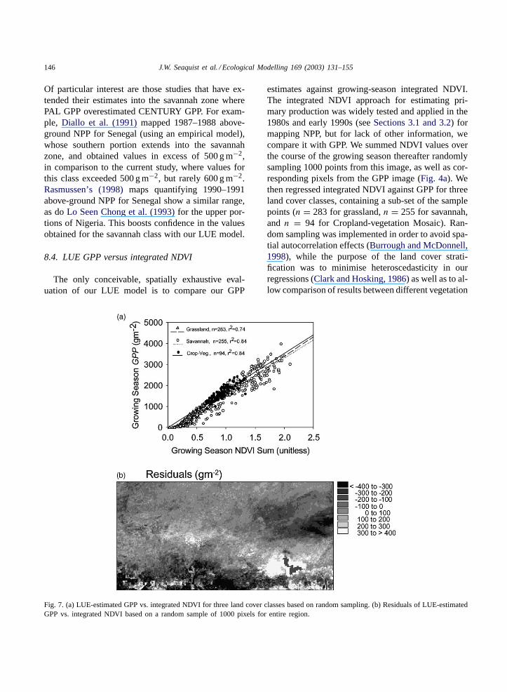
8.4. LUE GPP versus integrated NDVI

The only conceivable, spatially exhaustive eval-uation of our LUE model is to compare our GPP

Fig. 7. (a) LUE-estimated GPP vs. integrated NDVI for three land cover classes based on random sampling. (b) Residuals of LUE-estimatedGPP vs. integrated NDVI based on a random sample of 1000 pixels for entire region.

estimates against growing-season integrated NDVI.The integrated NDVI approach for estimating pri-mary production was widely tested and applied in the1980s and early 1990s (seeSections 3.1 and 3.2) formapping NPP, but for lack of other information, wecompare it with GPP. We summed NDVI values overthe course of the growing season thereafter randomlysampling 1000 points from this image, as well as cor-responding pixels from the GPP image (Fig. 4a). Wethen regressed integrated NDVI against GPP for threeland cover classes, containing a sub-set of the samplepoints (n = 283 for grassland,n = 255 for savannah,and n = 94 for Cropland-vegetation Mosaic). Ran-dom sampling was implemented in order to avoid spa-tial autocorrelation effects (Burrough and McDonnell,1998), while the purpose of the land cover strati-fication was to minimise heteroscedasticity in ourregressions (Clark and Hosking, 1986) as well as to al-low comparison of results between different vegetation

J.W. Seaquist et al. / Ecological Modelling 169 (2003) 131–155 147

units.Fig. 7ashows that while the regressions betweenGPP and integrated NDVI for the three land coverclasses are similar, a moderate amount of scatter isobserved withr2 values ranging from 0.74 (grassland)to 0.84 for the others. We then used the 1000 sampledpoints to regress growing season integrated NDVIagainst GPP for the entire region (r2 = 0.93), there-after using this equation to map the residuals from thisregression in terms of GPP, shown inFig. 7b. Despitethe overall high correlation between the two images,relatively large differences are notable, especially inareas of greater biomass. In his 1998 paper, Rasmussenconcluded that the spatial and temporal variation ofthe NPP-integrated NDVI relation stems from eithervariations in the biological growth efficiency, incon-sistent response of the NDVI to environmental and cli-matic influences, or a combination of both. It followsthat the unexplained variance in our GPP-integratedNDVI relation originates from the combined effectsof ε (water stress scalar) and PAR, and in particular,the soil characteristics regulating transpiration. We donot exploreRasmussen’s (1998)NDVI hypothesis inthis paper.

9. Discussion and conclusions

There are a number of LUE-type models of varyingcomplexity described in the literature, some of whichuse satellite data as a driver (e.g.Goetz et al., 1999),and others that are general enough to be applied to anumber of different biomes including grasslands (e.g.Running and Hunt, 1993). Some of these models aredesigned for simulating the primary production in offorest stands (e.g.Landsberg and Waring, 1997) whilemost that use remotely-sensed data operate in the spa-tial domain. Yet others have been developed especiallyfor semi-arid grasslands (Mougin et al., 1995). Wehave developed a model that yields estimates of grass-land primary production as a map. Our model is similarto some of the others to the extent that it is embeddedin a LUE framework. On a more detailed level, our ap-proach is unique because it considers solely the waterused by plants (actual transpiration) to index biologi-cal growth efficiency. This is particularly important forapplications in partially vegetated landscapes wherethe fate of precipitation is highly controlled by relativeamounts of vegetation. Our parameterisation of water

stress is both pragmatic (given the data limitations)and biophysically realistic. This has been accom-plished by subsuming classical and highly workablerangeland-yield formulations into our model (Eq. (3)).The combined use of the NDVI (Eqs. (4) and (5)),Ritchie’s (1972) model of bare soil evaporation(Appendix D), as well as a bucket model (Eqs. (7)–(9))facilitates this. After testing several other approachesfor deriving spatially explicit fields of actual evapo-transpiration (e.g. conventional bucket model wheretranspiration and bare soil evaporation are lumpedtogether), this logic yields the most realistic and con-sistent results (seeFig. 3e). Since primary productionin semi-arid rangelands is largely controlled by mois-ture limitations, this is an important part of our work.

Our model has merit because it has been devel-oped for applications in data-impoverished parts of theworld. These regions are often economically disad-vantaged and undergoing a diminution of the naturalresource base and are therefore in need of monitoring.Furthermore, recent evidence highlights the AfricanSahel as potentially important regulator of the tropi-cal carbon budget. The sophisticated techniques thathave become routine for accurately probing ecosys-tem processes in North America or Europe often can-not be supported over vast regions like the AfricanSahel. That we chose to develop our model for thisarea is motivated by such issues. We have therefore at-tempted to bridge gaps between data availability, rep-resentation of process, and model reliability, and spentsome effort developing, and profiling how we actu-ally derived the data layers in order to successfullyapply our LUE model. Our methods exemplify a cre-ative and efficient used sparse data set. Of particularsignificance is the use of the CLAVR layer from thePAL data set in order to derive, on a cell-by-cell ba-sis, several important parameters pertaining to energybalance, including global and photosynthetically ac-tive radiation, net radiation, and potential evapotran-spiration, among others. We have circumvented theneed for using output from general circulation mod-els, dense and extensive ground-based networks, orother data-intensive methods that rely on expensive orhard-to-get satellite data, and upon which other LUEmodels rely. Though ground data are lacking to pro-vide a formal validation for these variables in the WestAfrican Sahel, indications are, based on mean monthlyrelative sunshine duration computed across the region

148 J.W. Seaquist et al. / Ecological Modelling 169 (2003) 131–155

for available stations, little bias is incurred. However,we stress that the model could easily be applied in anygrassland region where more conventional and accu-rate data sources exist. Recently, our model has beensuccessfully applied, with slight modifications, to therangelands of Inner Mongolia (Runnström et al., 2001;Brogaard et al., forthcoming). This is a testament tothe general applicability and resiliency of our LUEmodel for other parts of the world.

Where possible, we have compared our derived vari-ables with ground data, or performed sensitivity testson various sub-models and components to ensure thatour model performed in a robust manner. This was ofmajor concern because formal validation is virtuallyimpossible given the nature of the region for whichwe developed our model. Though all our evaluationexercises were informative, we believe that the re-sults of the Monte Carlo simulations were particularlynovel, striking, and useful. For example, it allowed usto identify where (geographically) our model is mostlikely to be unreliable—along the fringe of the north-ern fringe of the Sahel belt. To the best of our knowl-edge, no research as regards the spatial modelling ofprimary production has displayed results in such amanner. Additionally, not only were we able to iden-tify those variables that contribute most to uncertaintyin our maps, but we also showed that the contributionof error from any one particular variable varied acrossspace, thus tipping the balance of error contributionfrom one variable to another from one sub-region toanother.

This work is part of a larger, ongoing effort to quan-tify and explain carbon budget dynamics in the Sahel,a region where considerable knowledge gaps exist. Im-minently, we are seeking to apply our LUE model tothe full extent of the NOAA AVHRR archive in orderquantify the inter-annual flow of carbon into the veg-etation, and elucidate its uncertainties. Ultimately, weaim to elucidate the role that the Sahel plays in thetropical carbon budget.

Acknowledgements

This work was funded by the Swedish InternationalDevelopment Agency, and the Swedish NationalSpace Board, while J.W. Seaquist was partly fundedby Natural Sciences Engineering and Research Coun-

cil of Canada. The Nordic-Africa Institute providedtravel funds for J.W. Sseaquist. We are indebted toA. Warren, H. Osbahr, N. Taylor, and M. Seyni forassistance during the initial data gathering stages ofthis research. I.L. Mouhamadou of the Niger Mete-orological Office in Niamey provided access to dailyclimate records. We thank A. Chappell and I. Clarkfor giving sound geostatistical advice. The help ofM. Runnström for the temporal downscaling of rain-fall is greatly appreciated. We also thank anonymousreferees for comments that improved our manuscript.The satellite information that we used includes dataproduced through funding from the Earth ObservingSystem Pathfinder Program of NASA’s Mission toPlanet Earth in cooperation with National Oceanic andAtmospheric Administration. The data were providedby the Earth Observing System Data and InformationSystem (EOSDIS), Distributed Active Archive Cen-ter at Goddard Space Flight Center which archives,manages, and distributes this data set.

Appendix A

The algorithm necessary for obtaining solar irradi-ance at the top of the atmosphere (So) may be obtainedfrom a number of different sources (e.g.Monteith andUnsworth, 1990; Shuttleworth, 1993; Haxeltine andPrentice, 1996). Each one varies in form dependinghow the parameters are lumped.

So = 24(60)

πQodr(ωs sinφ sinδ+ cosφ cosδ sinωs)

(A.1)

where So is the extraterrestrial irradiance (MJ m−2

day−1), Qo is the solar constant (0.0820 MJ m−2

min−1), dr is the relative Earth–Sun distance (unitless),ωs is the sunset hour angle,φ is the latitude—positivein the northern hemisphere, negative in the southern(radians), andδ is the solar declination (radians).

The relative Earth–Sun distance,dr, is:

dr = 1 + 0.033 cos

(2π

365J

)(A.2)

whereJ is the Julian day number.The sunset hour angle is given by:

ωs = arccos(−tanφ tanδ) (A.3)

J.W. Seaquist et al. / Ecological Modelling 169 (2003) 131–155 149

The solar declination is,δ, is:

δ = 0.4093 sin

(2π

365J − 1.405

)(A.4)

Ångström’s formula for computing the amount ofbroad-band (global) radiation reaching the Earth’s sur-face is:

St = So

[as + bs

(niN

)](A.5)

where St is the solar radiation reaching the Earth’ssurface (MJ m−2 day−1), So is the extraterrestrial ir-radiance (MJ m−2 day−1), as is the fraction of globalradiationSo on overcast days,as + bs is the fractionglobal radiation reaching the Earth’s surface on cleardays,ni is the sunshine duration (s), andN is the lengthof day (s).

The as andbs terms were tailored to West Africanconditions afterDavies (1966). ni/N is given a value of0 for CLAVR cells flagged as cloudy, while clear cellsreceive a value of 1. The mean value for the mixedcloud category, a priori unknown, was determined tobe 0.4 based on calibration against ground observa-tions of St from the HAPEX-Sahel experimental site(13◦32′N and 2◦39′E). Normalised root mean squareerrors of 15.69, 10.96, and 1.96% for 10-day, monthly,and yearly summation periods, respectively, were ob-tained (seeSeaquist and Olsson, 1999for details).Data on relative sunshine duration from nine stationsscattered throughout Niger show that little spatial biasin incurred in estimatedni/N (when compared to ob-served values ) and henceSt and PAR throughout theregion. PAR is taken to be 48% ofSt .

Appendix B

The bracketed terms containing NDVI and raised tothe exponent 2 inEqs. (4) and (5)are fractional veg-etation cover. NDVI is ‘re-normalised’ which offersthe following benefits: (1) numerical aesthetics; (2)insensitivity to viewing angle, sensor drift, and atmo-spheric contamination (Carlson et al., 1995). The termis then squared to obtain fractional vegetation cover(e.g. Choudhury et al., 1994; Carlson et al., 1995;Capehart, 1996; Carlson and Ripley, 1997). Ritchie(1972)expresses the energy available for phase 1 soilevaporation in terms of net radiation (Rn) and leaf areaindex (LAI). ReplacingRn with ETp:

Ep = ETp exp(−c × LAI ) (B.1)

whereEp is same as inEq. (8)(bare soil evaporation)(mm), ETp is same as inEq. (6)(potential evapotran-spiration) (mm), LAI is the Leaf Area Index, andc isthe empirical parameter (unitless).

Following Choudhury et al. (1994)andChoudhuryand DiGirolamo (1998), the fractional vegetationcover may be expressed as:

Fr = 1 − exp(G× LAI ) (B.2)

where Fr is the fractional vegetation cover (unitless),G is the value determined by leaf angle distribution.

Combining (D.1) and (D.2) yields:

Ep = ETp(1 − Fr)c/G (B3)

such thatc/G ≈ 1. This yieldsEq. (8), and its in-verse,Eq. (9). The derivation followsChoudhury andDiGirolamo (1998).

Appendix C

Net radiation is the sum net long-wave and netshort-wave radiation (Shuttleworth, 1993):

Rn = St(1 − αs)− fε′nσ(T + 273.2)4 (C.1)

whereRn is the net radiation (MJ m−2 day−1), St issame as inAppendix A, αs is the surface albedo (unit-less),f is the adjustment for cloud cover (unitless),ε′is the net emissivity between the atmosphere and theground (unitless),σ is the Stefan-Boltzmann constant(4.903× 10−9 MJ m−2 K−4 day−1), n is the numberof days in the month, andT is the monthly mean airtemperature (◦C).

An adjustment for cloud cover,f, was determinedas a by-product of the PAR (St) computation inAppendix A(Shuttleworth, 1993):

f =(ac

bs

as + bs

)ni

N+

(bc + as

as + bsac

)(C.2)

where as is the constant as inEq. (A.5), bs is theconstant as inEq. (A.5), ni is the sunshine durationas in Eq. (A.5), N is the day-length as inEq. (A.5),ac = 1.35, andbc = −0.35.

The ac andbc coefficients are calibration parame-ters determined from measurements of long-wave ra-diation. For arid environments, the above values arerecommended.

150 J.W. Seaquist et al. / Ecological Modelling 169 (2003) 131–155

The net emissivity between the atmosphere and theground was computed according to the following, asdata for vapour pressure, dew point, and humidity wereunavailable (Shuttleworth, 1993):

ε′ = −0.02+ 0.261 exp(−7.77× 10−4 T−2) (C.3)

whereε′ is the net emissivity between the atmosphereand the land surface (unitless), andT is the monthlymean temperature in◦C.

According to Song and Gao (1999)broad-bandalbedo may be recovered from the spectral-specificalbedos by a linear combination of the RED and NIRchannels of the NOAA AVHRR sensor:

αp = β1RED+ β2NIR + χ (C.4)

whereαp is the planetary albedo (unitless), RED isthe AVHRR channel 1 reflectance (unitless), NIR isthe AVHRR channel 2 reflectance (unitless),β1 is theempirically derived coefficient,β2 is the empiricallyderived coefficient, andχ = 0.

Both β1 andβ2 are affected by vegetation amount,and are ‘calibrated’ by the NDVI:

β1 = 0.494NDVI2 − 0.329NDVI + 0.372 (C.5)

β2 = −1.439NDVI2 + 1.209NDVI + 0.587 (C.6)

Chen and Ohring (1984)empirically derived a so-lar zenith angle-dependent relation between planetaryalbedo derived from the NOAA AVHRR and surfacealbedo:

αp = a+ bαs (C.7)

whereαp is the planetary broad-band albedo,a is theconstant depending on solar zenith angle,b is the con-stant depending on solar zenith angle, andαs is thesurface broad-band albedo.

The equation was re-arranged forαs, and a look-uptable given inChen and Ohring (1984)was used todefine a and b for solar zenith angle ranges.Chenand Ohring (1984)report root mean square errors ofbetween 0.017 and 0.021 for solar zenith angles of 0and 85◦, respectively.

Appendix D

Before running the bucket model, we required anestimate ofEa (Eq. (7)), which we derived by applying

the two-stage evaporation model ofRitchie (1972).Ritchie’s model has been widely tested, especially atthe plot scale (e.g.Wight and Hanks, 1981; Brutsaertand Chen, 1995; Wallace and Holwill, 1997; Wallaceet al., 1999) but its application on regional or globalscales is limited toChoudhury and DiGirolamo(1998).

In Ritchie’s two-stage model, the first stage of baresoil evaporation occurs in the wake of a rainfall event,where soil evaporation is limited by the potential evap-oration at the soil surface. This stage proceeds untilthe cumulative evaporation reaches a threshold (t1) af-ter which the de-sorption phase (stage 2) dominates.At this stage, the rate of evaporation depends on thesquare root of time and the hydraulic properties of thesoil:

∑Es1 =

t1∑i=0

Epr = U, t < t1 (D.1)

∑Es2 = k × √

t − t1, t > t1 (D.2)

Ea =∑

Es1 +∑

Es2 (D.3)

where∑

Es1 is stage 1 cumulative soil evaporation(mm),

∑Es2 is stage 2 cumulative soil evaporation

(mm),∑

Eso is the potential evaporation for soil(mm), U is the total amount of water evaporated set-ting the upper limit for stage 1 evaporation (mm),kis the desorptivity mm day−1/2, and Ea is the actualevaporation (mm).

In plot-based studies, the constantsU andk are usu-ally determined empirically (e.g.Ritchie, 1972) anddepend on soil properties. They have been shown torangek = 3.34 (U = 6) for sandy soils tok = 5.08(U = 12) for clay loams. According toLe Houerou(1980)the overwhelming majority of the soils in Nigerare sandy, though black clayey soils (vertisols) mayoccur in local depressions. We therefore assigned val-ues ofk = 3.5 andU = 6, keeping in mind that soilsthroughout the region are composed mostly of sandwith local occurrences of black clay. Thek andU con-stants for sandy soils and black clays are very similar,based on the work ofRitchie (1972)andBlack et al.(1969). Unlike Ritchie’s original model, we ignoredthe impact of shading (acting to suppress vapour pres-sure deficit and wind speed) as this had an insignifi-cant impact on our final results.

J.W. Seaquist et al. / Ecological Modelling 169 (2003) 131–155 151

Appendix E

An important prerequisite for the use ofRitchie’s(1972) model for bare soil evaporation is that dailyrainfall records are available. The statistical down-scaling of rainfall from monthly to daily values isnot trivial, especially for spatially distributed rainfallfields. Weather generators can achieve this (e.g.Jonesand Thornton, 1997; Friend, 1998). We adopted asimpler approach. We inspected cumulative monthlyfrequency histograms of daily rainfall data for 15 sta-tions across Niger. For most stations during the rainyseason (defined here as May–October), over 50% ofthe rainfall that fell in each month occurred in short,intense bursts, between one and three times (roundedoff to the nearest whole number). The low magni-tude events comprised the lower 5% of the rainfalltotals and occurred between two and five times. Theremaining 45% of the rainfall occurred between twoand six times. Accordingly, the interpolated monthlytotal rainfall surfaces were divided into three cate-gories, comprising 5, 45 and 50% of the monthly to-tals. Rainfall events were treated as a time-dependentrandom process (using a random number generatorin FORTRAN), and no restrictions were made asregards the number of rainfall events of a given mag-nitude occurring within a cell on a given pseudo-day.Re-aggregation of the daily rainfall for the entire areato monthly totals faithfully reproduced the monthlyrainfall surfaces and verified the consistency of ourmethod.

Appendix F

We tested the impact on computedEa aggregatedover a 37-day period by artificially partitioning dailyrainfall as inAppendix Dwith the rainfall andEa dataset provided byRitchie (1972). Use of the actual rain-fall series produced a totalEa of 60.6 mm, whereasthe simulated rainfall series gave 57.4 mm, an under-estimation of 5.3%.

References

Africa Data Dissemination Service (ADDS) of the USGS,http://edcsnw4.cr.usgs.gov/adds/adds.html.

Agnew, C.T., Chappell, A., 1999. Drought in the Sahel. GeoJournal70, 299–311.

Ångström, A., 1924. Solar and terrestrial radiation. Q. J. R. Met.Soc. 50, 121–126.

Ardö, J., Olsson, L., 2002. Assessment of soil organic carbon insemi-arid Sudan using GIS and the CENTURY model. J. AridEnv. 54, 633–651.

Bartholome, E., 1990. Estimation of APAR values from AVHRRNDVI for regional crop yield assessment in West Africa. In:Proceedings of IGARSS’90 Symposium Technologies for theNineties, Washington, DC, May 21–24, 1990, pp. 587–590.

Bastiaanssen, W.G.M., 1995. Regionalization of Surface FluxDensities and Moisture Indicators in Composite Terrain—ARemote Sensing Approach Under Clear Skies in MediterraneanClimates. Ph.D. Thesis, Winand Staring Centre, Wageningen,The Netherlands, 273 pp.

Begue, A., 1993. Leaf area index, intercepted photosyntheticallyactive radiation, and spectral vegetation indices: a sensitivityanalysis for regular-clumped canopies. Rem. Sens. Env. 46,45–59.

Begue, A., Desprat, J.F., Imbernon, J., Baret, F., 1991. Radiationuse efficiency of pearl millet in the Sahelian zone. Agric. For.Met. 56, 93–110.

Black, T.A., Gardner, W.R., Thurtell, G.W., 1969. The predictionof evaporation, drainage, and soil water storage for a bare soil.Soil Sci. Soc. Am. Proc. 33, 655–660.

Box, E.O., Holben, B.N., Kalb, V., 1989. Accuracy of theAVHRR Vegetation Index as a predictor of biomass, primaryproductivity, and net CO2 flux. Vegetatio 80, 71–89.

Brogaard, S., Runnström, M., Seaquist, J.W., forthcoming. Primaryproduction of Inner Mongolia, China, between 1982 and 1999estimated by a satellite data-driven light use efficiency model.Submitted for publication.

Bromberg, J.G., McKeown, R., Knapp, L., Kittel, T.G.F., Ojima,D.S., 1996. Integrating GIS and the CENTURY model tomanage and analyse data. GIS and Environmental Modeling:Progress and Research Issues 429–431.

Brutsaert, W., Chen, D., 1995. Desorption and the two stagesof drying of natural tallgrass prairie. Water Resour. Res. 31,1305–1313.

Burke, I.C., Yonker, C.M., Cole, C.V., Flach, K., Schimel, D.S.,1989. Texture, climate, and cultivation effects on soil organicmatter context in U.S. grassland soils. Soil Sci. Soc. Am. J.53, 800–805.

Burrough, P.A., McDonnell, R.A., 1998. Principles of GeographicInformation Systems. Oxford University Press, 333 pp.

Capehart, W.J., 1996. Issues Regarding the Remote Sensing andModeling of Soil Moisture for Meteorological Applications.Ph.D. Thesis, Earth Systems Science Center, Pennsylvania StateUniversity, 238 pp.

Carlson, T.N., Ripley, D.A., 1997. On the relation between NDVI,fractional vegetation cover, and leaf area index. Rem. Sens.Env. 62, 241–252.

Carlson, T.N., Capehart, W.J., Gillies, R.R., 1995. A newlook at the simplified method for remote sensing of dailyevapotranspiration. Rem. Sens. Env. 54, 161–167.

CESBIO, ORSTOM, CNES, 1997. HAPEX-Sahel InformationSystem,http://www.ird.fr/hapex/.

152 J.W. Seaquist et al. / Ecological Modelling 169 (2003) 131–155

Chappell, A., Seaquist, J.W., Eklundh, L., 2001. Improving theestimation of noise from NOAA AVHRR NDVI for Africausing geostatistics. Int. J. Rem. Sens. 22, 1067–1080.

Chen, T.S., Ohring, G., 1984. On the relationship between clear-skyplanetary and surface albedo. J. Atmos. Sci. 41, 156–158.

Cherchali, S., Amram, O., Flouzat, G., 1995. The improvementof net primary productivity estimation taking into accountthe heterogeneity of Sahelian region. In: Proceedings ofIGARSS’95, Firenze, Italy, July 12–14, 1995, pp. 1230–1233.

Choudhury, B.J., 1994. Synergism of multispectral satelliteobservations for estimating regional land surface evaporation.Rem. Sens. Env. 49, 264–274.

Choudhury, B.J., DiGirolamo, N.E., 1998. A biophysicalprocess-based estimate of global land surface evaporation usingsatellite and ancillary data. I. Model description and comparisonwith observations. J. Hydrol. 205, 164–185.

Choudhury, B.J., Ahmed, N.U., Idso, S.B., Reginato, R.J.,Daughtry, C.S.T., 1994. Relations between evaporationcoefficients and vegetation indices studied by modelsimulations. Rem. Sens. Env. 50, 1–17.

Clark, W.A.V., Hosking, P.L., 1986. Statistical Methods forGeographers. Wiley, 518 pp.

Cole, C.V., Stewart, J.W.B., Ojima, D.S., Parton, W.J., Schimel,D.S., 1989. Modelling land use effects of soil organic matterdynamics in the North American Great Plains. In: Clarholm,M., Bergström, L. (Eds.), Ecology of Arable Land. KluwerAcademic Publishers, Amsterdam, The Netherlands, pp. 89–98.

Coops, N.C., Waring, R.H., Brown, S.R., Running, S.W., 2001.Comparisons of predictions of net primary production andseasonal patterns in water use derived with two forest growthmodels in Southwestern Oregon. Ecol. Model. 142, 61–81.

Crosetto, M., Ruis, J.A.M., Crippa, B., 2001. Uncertaintypropagation in models driven by remotely sensed data. Rem.Sens. Env. 76, 373–385.

Davies, J.A., 1966. The assessment of evapotranspiration forNigeria. Geogr. Ann. 48A, 139–166.

Diallo, O., Diouf, A., Hanan, N.P., Ndiaye, A., Prevost, Y., 1991.AVHRR monitoring of savannah primary production in Senegal,West Africa: 1987–1988. Int. J. Rem. Sens. 12, 1259–1280.

Eklundh, L., 1996. AVHRR NDVI for Monitoring and Mappingof Vegetation and Drought in East African Environments.Meddelanden från Lunds Universitets Geografiska Institutioner,Avhandlingar, pp. 126, 187.

Eklundh, L., Olsson, L., 2003. Vegetation index trends for theAfrican Sahel 1982–1999. Geophys. Res. Lett. 30, 1430,doi:10.1029/2002GL016772.

FAO/UNESCO, 1995. Digital Soil Map of the World and DerivedProperties Version 3.5. Food and Agriculture Organization ofthe United Nations.

Field, C.B., Randerson, J.T., Malmström, C.M., 1995. Global netprimary production: combining ecology and remote sensing.Rem. Sens. Env. 51, 74–88.

Friend, A.D., 1998. Parameterisation of a global daily weathergenerator for terrestrial ecosystem modelling. Ecol. Model. 109,121–140.

Frouin, R., Pinker, R.T., 1995. Estimating photosyntheticallyactive radiation (PAR) at the Earth’s surface from satelliteobservations. Rem. Sens. Env. 51, 98–107.

Goetz, S.J., Prince, S.D., 1999. Modelling terrestrial carbonexchange and storage: evidence and implications of functionalconvergence light use efficiency. Adv. Ecol. Res. 28, 57–92.

Goetz, S.J., Prince, S.D., Goward, S.N., Thawley, M.M., Small,J., 1999. Satellite remote sensing of primary production:an improved production efficiency modeling approach. Ecol.Model. 122, 239–255.

Goovaerts, P., 1997. Geostatistics for Natural Resource Evaluation.Oxford University Press, 483 pp.

Goward, S.M., Huemmrich, K.E., 1992. Vegetation canopy PARabsorptance and the Normalized Difference Vegetation Index:an assessment using the SAIL model. Rem. Sens. Env. 39,119–140.

Gower, S.T., Kucharik, C.J., Norman, J.M., 1999. Direct andindirect estimation of leaf area index, FAPAR, and net primaryproduction of terrestrial ecosystems. Rem. Sens. Env. 70, 29–51.

Guerif, M., de Brisis, S., Seguin, B., 1993. CombinedNOAA-AVHRR and SPOT-HRV data for assessing crop yieldsof semi-arid environments. EARSeL Adv. Rem. Sens. 2, 110–123.

Hall, D.O., Rao, K.K., 1994. Photosynthesis. Cambridge UniversityPress, 211 pp.

Hanan, N.P., Prince, S.D., Begue, A., 1995. Estimation ofabsorbed photosynthetically active radiation and vegetation netproduction efficiency using satellite data. Agric. For. Met. 76,259–276.

Hanan, N.P., Prince, S.D., Begue, A., 1997. Modelling vegetationprimary production during HAPEX-Sahel using productionefficiency and canopy conductance model formulations. J.Hydrol. 188/189, 651–675.

Handcock, R., 2001. Spatio-Temporal Analysis of Net PrimaryProduction Across Ontario Using an Ecoregionalization. Ph.D.Thesis, University of Toronto, Toronto, Ont., Canada, 150 pp.

Hanks, R.J., 1974. Model for predicting plant yield as influenceduse. Agron. J. 66, 660–665.

Haxeltine, A., Prentice, I.C., 1996. BIOME3: an equilibriumterrestrial biosphere model based on ecophysiologicalconstraints, resource availability, and competition among plantfunctional types. Glob. Biogeochem. Cycles 10, 693–709.

Heuvelink, G.B.M., 1998. Error Propagation in EnvironmentalModelling with GIS. Taylor & Francis, London, 127 pp.

Holben, B.N., 1986. Characteristics of maximum-value compositeimages from temporal AVHRR data. Int. J. Rem. Sens. 7, 1417–1437.

Hulme, M., 1989. Is environmental degradation causing droughtin the Sahel? An assessment from recent empirical research.Geography 38–46.

Hunt Jr., E.R., 1994. Relationship between woody biomass andPAR conversion efficiency for estimating net primary productionfrom NDVI. Int. J. Rem. Sens. 15, 1725–1730.

James, M.E., Kalluri, S.N.V., 1994. The Pathfinder AVHRR landdata set: an improved coarse resolution data set for terrestrialmonitoring. Int. J. Rem. Sens. 15, 3347–3363.

Jensen, R.E., Burman, R.D., Allen, R.G., 1990. Evapotranspirationand irrigation water requirements. ASCE Manual 70, 332.

Jiang, L., Islam, S., 1999. A methodology for estimation ofsurface evapotranspiration over large areas using remote sensingobservations. Geophys. Res. Lett. 26, 2773–2776.

J.W. Seaquist et al. / Ecological Modelling 169 (2003) 131–155 153

Jones, P.G., Thornton, P.K., 1997. Spatial and temporal variabilityof rainfall related to a third-order Markov model. Agric. For.Met. 86, 127–138.

Justice, C.O., Hiernaux, P.H.Y., 1986. Monitoring the grasslandsof the Sahel using NOAA AVHRR data: Niger 1983. Int. J.Rem. Sens. 7, 1515–1532.

Kaisischke, E.S., French, N.H.F., 1997. Constraints on usingAVHRR composite index imagery to study patterns ofvegetation cover in boreal forest. Int. J. Rem. Sens. 18, 2403–2426.

Kaufman, Y.J., Tanre, D., 1996. Strategy for direct and indirectmethods for correcting the aerosol effect on remote sensing:from AVHRR to EOS-MODIS. Rem. Sens. Env. 55, 65–79.

Kimball, J.S., White, M.A., Running, S.W., 1997. BIOME-BGCsimulations of stand hydrologic processes for BOREAS. J.Geophys. Res. 102 (D24), 29043–29051.

L’homme, J.-P., 1996. A theoretical basis for the Priestley-Taylorcoefficient. Boundary Layer Met. 82, 179–191.

Landsberg, J.J., Waring, R.H., 1997. A generalised model offorest productivity using simplified concepts of radiation-useefficiency, carbon balance and partitioning. For. Ecol. Manage.95, 209–228.

Le Houerou, H.N., 1980. The rangelands of the Sahel. J. RangeManage. 33, 41–46.

Le Houerou, H.N., Popov, G.F., See, L., 1993. Agro-BioclimaticClassification of Africa. Working Paper Number 6, FAOMeteorology Series.

Lind, M., Fensholt, R., 1999. The spatio-temporal relationshipbetween rainfall and vegetation development in Burkina Faso.Danish J. Geog. (Special Issue 2), 43–55.

Lobell, D.B., Hicke, J.A., Asner, G.P., Field, C.B., Tucker, C.J.,Los, S.O., 2002. Satellite estimates of productivity and lightuse efficiency in United States agriculture, 1982–1998. Glob.Chem. Biol. 8, 722–735.

Lo Seen Chong, D., Mougin, E., Gastellu-Etchegorry, J.P., 1993.Relating the Global Vegetation Index to net primary productivityand actual evapotranspiration over Africa. Int. J. Rem. Sens.14, 1517–1546.

Loveland, T.R., Zhu, Z., Ohlen, D.O., Brown, J.F., Reed, B.C.,Yang, L., 1999. An analysis of the IGBP global land-covercharacterization process. Photogr. Eng. Rem. Sens. 65, 1021–1032.

Maisongrande, P., Ruimy, A., Dedieu, G., Saugier, B., 1995.Monitoring seasonal and interannual variations of gross primaryproductivity, net primary productivity and net ecosystemproductivity using a diagnostic model and remotely-sensed data.Tellus 47B, 178–190.

Maselli, F., Conese, C., Petkov, L., Gilabert, M.A., 1992. Use ofNOAA-AVHRR NDVI data for environmental monitoring andcrop forecasting in the Sahel. Preliminary results. Int. J. Rem.Sens. 14, 2743–2749.

Matheron, M.A., 1971. The Theory of Regionalized Variables andIts Applications, vol. 5. Centre de Morpholgie Mathematiquede Fountainbleau, Fountainebleau.

Metherell, A.K., Harding, L.A., Cole, C.V., Parton, W.J., 1993.CENTURY Soil Organic Matter Environment, TechnicalDocumentation, Agroecosystem Version 4.0. United States

Department of Agriculture, Agricultural Research Service,Great Plaines System Research Unit. Technical Report #4.

Mikhailova, E.A., Bryant, R.B., DeGloria, S.D., Post, C.J.,Vessenev, I.I., 2000. Modeling soil organic matter dynamicsafter conversion of native grassland to long-term continuousfallow using the CENTURY model. Ecol. Model. 132, 247–257.

Millington, A.C., Wellens, J., Settle, J.J., Saull, R.J., 1994.Explaining and monitoring land cover dynamics in drylandsusing multitemporal analysis of NOAA AVHRR imagery. In:Foody, G., Curran, P. (Eds.), Environmental Remote Sensingfrom Regional to Global Scales. Wiley, Chechester, pp. 16–43.

Monteith, J.L., 1972. Solar radiation and productivity in tropicalecosystems. J. Appl. Ecol. 9, 747–766.

Monteith, J.L., 1977. Climate and the efficiency of crop productionin Britain. Phil. Trans. R. Soc. Lond. 281, 277–294.

Monteith, J.L., Unsworth, M., 1990. Principles of EnvironmentalPhysics. Arnold, London, 291 pp.

Mougenot, B., Begue, A., Chehbouni, G., Escadafal, R., Heilman,P., Qi, J., Royer, A., Watts, C., 2000. Applications ofVEGETATION Data to Resource Management in Arid andSemi-Arid Rangelands. 7 pp.

Mougin, E., Lo Seen, D., Rambal, S., Gaston, A., Hiernaux, P.,1995. A regional Sahelian grassland model to be coupled withmultispectral satellite data. I. Model description and validation.Rem. Sens. Env. 52, 181–193.

Myneni, R.B., Williams, D.L., 1994. On the relationship betweenFAPAR and NDVI. Rem. Sens. Env. 49, 200–211.

Nicholson, S.E., Lare, A.R., Marengo, J.A., Santos, P., 1996. Arevised version of Lettau’s evapoclimatonomy model. J. Appl.Met. 35, 549–561.

Nicholson, S.E., Tucker, C.J., Ba, M.B., 1998. Desertification,drought, and surface vegetation: an example from the WestAfrican Sahel. Bull. Am. Met. Soc. 79, 815–829.

Olsson, L., 1993. Desertification in Africa—a critique and analternative approach. GeoJournal 31, 23–31.

Parton, W.J., Schimel, D.S., Cole, C.V., Ojima, D.S., 1987.Analysis of factors controlling soil organic levels of grasslandsin the Great Plains. Soil Sci. Soc. Am. J. 51, 1173–1179.

Parton, W.J., Stewart, J.W.B., Cole, C.V., 1988. Dynamics of C,N, P, and S in grassland soils: a model. Biogeochemistry 5,109–131.

Parton, W.J., Scurlock, J.M.O., Ojima, D.S., Gilmanov, T.G.,Scholes, R.J., Schimel, D.S., Kirchner, T., Menaut, J.-C.,Seastedt, T., Moya, E.G., et al., 1993. Observations andmodelling of biomass and soil organic matter dynamics forthe grassland biome worldwide. Glob. Biogeochem. Cycles 7,785–809.

Parton, W.J., Ojima, D.S., Schimel, D.S., 1994. Environmentalchange in grasslands: assessment using models. Clim. Change28, 111–114.

Parton, W.J., Coughenour, M.B., Scurlock, J.M.O., Ojima, D.S.,Gilmanov, T.G., Scholes, R.J., Schimel, D.S., Kirchner, T.B.,Menaut, J.-C., Seastedt, T.R., et al. 1996. Global grasslandecosystem modelling: development and test of ecosystemmodels for grassland ecosystems. In: Breymeyer, A.I., Hall,D.O., Mellilo, J.M., Ågren, G.I. (Eds.), Global Change: Effectson Coniferous Forests and Grasslands. Wiley, New York,pp. 229–279.

154 J.W. Seaquist et al. / Ecological Modelling 169 (2003) 131–155

Potter, C.S., Randerson, J.T., Field, C.B., Matson, P.A.,Vitousek, P.M., Mooney, H.A., Klooster, S.A., 1993. Terrestrialecosystem production: a process model based on globalsatellite and surface data. Glob. Biogeochem. Cycles 7, 811–841.

Priestley, C.H.B., Taylor, R.J., 1972. On the assessment of surfaceheat flux and evaporation using large-scale parameters. MonthlyWeather Rev. 100, 81–92.

Prince, S.D., 1991a. Satellite remote sensing of primary production:comparison of results for Sahelian grasslands 1981–1988. Int.J. Rem. Sens. 12, 1301–1312.

Prince, S.D., 1991b. A model of regional primary production foruse with coarse resolution satellite data. Int. J. Rem. Sens. 12,1313–1330.

Prince, S.D., Goward, S.N., 1995. Global primary production: aremote sensing approach. J. Biogeogr. 22, 815–835.

Prince, S.D., Kerr, Y.H., Goutorbe, J.-P., Lebel, T., Tinga, A.,Bessemoulin, P., Brouwer, J., Dolman, A.J., Engman, E.T.,Gash, J.H.C., Hoepffner, M., Kabat, P., Monteny, B., Said, F.,Sellers, P., 1995. Geographical, biological, and remote sensingaspects of the hydrologic atmospheric pilot experiment in theSahel (HAPEX-Sahel). Rem. Sens. Env. 51, 215–234.

Prince, S.D., Brown de Coulstoun, E., Kravitz, L.L., 1998.Evidence from rain-use efficiencies does not indicate extensiveSahelian desertification. Glob. Change. Biol. 4, 359–374.

Rasmussen, M.S., 1998. Developing simple, operational, consistentNDVI-vegetation models by applying environmental andclimatic information. Part I. Assessment of net primaryproduction. Int. J. Rem. Sens. 19, 97–117.

Ruimy, A., Dedieu, G., Saugier, B., 1996. TURC: a diagnosticmodel of continental gross primary productivity and net primaryproductivity. Glob. Biogeochem. Cycles 10, 269–286.

Reeves, M.C., Winslow, J.C., Running, S.W., 2001. Mappingweekly rangeland vegetation productivity using MODISalgorithms. J. Range Manage. 54, 90–105.

Ritchie, J.T., 1972. Model for predicting evaporation from a rowcrop with incomplete cover. Water Resour. Res. 8, 1204–1213.

Rockström, J., 1997. On-Farm Agrohydrological Analysis of theSahelian Yield Crisis: Rainfall Partitioning, Soil Nutrients,and Water Use Efficiency of Pearl Millet. Akademitryck AB,Stockholm.

Rosema, A., 1993. Using METEOSAT for operationalevapotranspiration and biomass monitoring in the Sahel region.Rem. Sens. Env. 46, 27–44.

Ruimy, A., Dedieu, G., Saugier, B., 1996. TURC—TerrestrialUptake and Release of Carbon by vegetation: a diagnosticmodel of continental gross primary productivity and netprimary productivity. Glob. Biogeochem. Cycles 10, 269–285.

Running, S.W., Hunt Jr., E.R., 1993. Generalization of a forestecosystem process model for other biomes, BIOME-BGC, andan application for global-scale models. In: Ehleringer, J.R.,Field, C. (Eds.), Scaling Processes Between Leaf and LandscapeLevels. Academic Press, pp. 141–158.

Runnström, R., Brogaard, S., Seaquist, J.W., 2001. Asatellite data-driven parametric model of primary productionimplemented over the inner Mongolian rangeland of northern

China. In: Challenges of a Changing Earth: A Global ChangeOpen Science Conference, Amsterdam, July 10–13, 2001(Category: Sustaining the Land: Food, Biodiversity, and OtherServices).

Runyon, J., Waring, R.H., Goward, S.N., Welles, J.M., 1994.Environmental limits on net primary production and light-useefficiency across the Oregon transect. Ecol. Appl. 4, 226–237.

Schimel, D.S., et al., 2001. Recent patterns and mechanisms ofcarbon exchange by terrestrial ecosystems. Nature 414, 169–172.

Seaquist, J.W., 2001. Mapping Primary Production for the WestAfrican Sahel with Satellite Data. Ph.D. Thesis, Meddelandenfran Lunds Universitets Geografiska Institutioner, Avhandlingar,pp. 140, 198.

Seaquist, J.W., Olsson, L., 1999. Rapid estimation of photo-synthetically active radiation over the West African Sahel usingthe Pathfinder Land Data Set. Int. J. Earth Obs. Geoinf. 1,205–213.

Shuttleworth, W.J., 1993. Evaporation. In: Maidment, D.R. (Ed.),Handbook of Hydrology. McGraw-Hill, New York.

Smith, P.M., Kalluri, S.N.V., Prince, S.D., DeFries, R., 1997a.The NOAA/NASA Pathfinder AVHRR 8-km Land Data Set.Photogram. Eng. Rem. Sens. LXIII, 12–32.

Smith, P., Smith, J.U., Powlson, D.S., McGill, W.B., Arah,J.R.M., Chertov, O.G., Coleman, K., Frankoe, U., Frolkning, S.,Jenkinson, D.S., et al., 1997b. A comparison of the performanceof nine soil organic matter models using data sets from sevenlong-term experiments. Geoderma 81, 153–225.

Song, J., Gao, W., 1999. An improved method to derive surfacealbedo from narrowband AVHRR satellite data: narrowband tobroadband conversion. J. Appl. Met. 38, 239–249.

Soufflet, V., Tanre, D., Begue, A., Podaire, A., Deschamps, P.Y.,1991. Atmospheric effects on NOAA/AVHRR imagery overSahelian regions. Int. J. Rem. Sens. 12, 1189–1203.

Srivastava, S.K., Jayaraman, V., Nageswara Rao, P.P.,Manikiam, B., Chandrasekhar, M.G., 1997. Interlinkagesof NOAA/AVHRR derived integrated NDVI to seasonalprecipitation and transpiration in dryland tropics. Int. J. Rem.Sens. 18, 2931–2952.

Tucker, C.J., Vanpraet, C., Boerwinkel, E., Gaston, A., 1983.Satellite remote sensing of total dry matter production in theSenegalese Sahel. Rem. Sens. Env. 13, 461–474.

Tucker, C.J., Vanpraet, C.L., Sharman, M.J., van Ittersum, G., 1985.Satellite remote sensing of total herbaceous biomass productionin the Senegalese Sahel: 1980–1984. Rem. Sens. Env. 17, 233–250.

USGS EROS Data Center Distributed Archive Center, 2000.Africa Land Cover Characteristics Data Base Version 1.2 athttp://edcdaac.usgs.gov/glcc/tabgoodeaf.html.

Veroustraete, F., Patyn, J., Myneni, R.B., 1996. Estimating netecosystem exchange of carbon using the normalized differencevegetation index and an ecosystem model. Rem. Sens. Env. 58,115–130.

Verstraete, M.M., Pinty, B., 1991. The potential contribution ofsatellite remote sensing to the understanding of arid landsprocesses. Vegetatio 91, 59–72.

J.W. Seaquist et al. / Ecological Modelling 169 (2003) 131–155 155

Viovy, N., Arino, O., Belward, A.S., 1992. The best index slopeextraction (BISE): a method for reducing noise in NDVItime-series. Int. J. Rem. Sens. 13, 1585–1590.

Vose, R.S., Schmoyer, R.L., Steurer, P.M., Peterson, T.C.,Heim, R., Karl, T.R., Eischeid, J.K., 1992. The globalhistorical climatology network: long-term monthly temperature,precipitation, sea level pressure, and station pressuredata version 2.0,http://cdiac.esd.ornl.gov/epubs/ndp/ndp041/ndp041.html.

Wallace, J.S., Holwill, C.J., 1997. Soil evaporation from tiger-bushin south-west Niger. J. Hydrol. 188/189, 426–442.

Wallace, J.S., Lloyd, C.R., Sivakumar, M.V.K., 1993.Measurements of soil, plant, and total evaporation from milletin Niger. Agric. For. Met. 63, 149–169.

Wallace, J.S., Jackson, N.A., Ong, C.K., 1999. Modelling soilevaporation in an agroforestry system in Kenya. Agric. For.Met. 94, 189–202.

White, J.D., Running, S.W., 1994. Testing scale dependentassumptions in regional ecosystem simulations. J. Veg. Sci. 5,687–702.

Wight, J.R., Hanks, R.J., 1981. A water-balance, climate modelfor range herbage production. J. Range Manage. 34, 307–311.

Wylie, B.K., Harrington, J.A., Prince, S.D., Denda, I., 1991.Satellite and ground-based pasture production assessment inNiger: 1986–1988. Int. J. Rem. Sens. 12, 1281–1300.

Wythers, K.R., Laurenroth, W.K., Paruelo, J.M., 1999. Bare-soilevaporation under semiarid field conditions. Soil Sci. Am. J.63, 1341–1349.