A regularization term to avoid thesaturation of the sigmoids in multilayerneural networks �Lluis Garrido1;2, Sergio G�omez1 y,Vicens Gait�an2 and Miquel Serra-Ricart31) Dept. d'Estructura i Constituents de la Mat�eria,Facultat de F��sica, Universitat de Barcelona,Diagonal 647, E-08028 Barcelona, Spain.2) Institut de F��sica d'Altes Energies,Universitat Aut�onoma de Barcelona,E-08193 Bellaterra (Barcelona), Spain.3) Instituto de Astrof��sica de CanariasE-38200 La Laguna (Tenerife), Spain.AbstractIn this paper we propose a new method to prevent the saturation ofany set of hidden units of a multilayer neural network. This method is im-plemented by adding a regularization term to the standard quadratic errorfunction, which is based on a repulsive action between pairs of patterns.Published in International Journal of Neural Systems 7 (1996) 257{262.�This research is partly supported by the `Comissionat per Universitats i Recerca de laGeneralitat de Catalunya' and by EU under contract number CHRX-CT92-0004yPresent address: Dept. d'Enginyeria Inform�atica (ETSE), Univ. Rovira i Virgili, Crt. deSalou s/n (Complex educatiu), E-43006 Tarragona (Spain)1

1 IntroductionConsider a multilayer neural network consisting of L layers with n1, . . . , nL unitsrespectively. The equations governing the state of the net are�(`)i = g n`�1Xj=1 !(`)ij �(`�1)j � �(`)i ! ; i = 1; : : : ; n` ; ` = 2; : : : ; L ; (1.1)where �(`) represents the state of the neurons in the `-th layer, f!(`)ij g the weightsbetween units in the (`� 1)-th and the `-th layers, �(`)i the threshold of the i-thunit in the `-th layer, and g is the activation function, usually taken to be thesigmoid g(h) = 11 + e�h : (1.2)This kind of network may be seen as a composition of `� 1 functions:Rn1 f(2)�! [0; 1]n2 f(3)�! [0; 1]n3 �! � � � f(L)�! [0; 1]nLTherefore, if we have a certain set of input patterns fx� 2 Rn1 ; � = 1; : : : ; pg,we can study how the shape of the distribution changes when it is introduced inthe net.The parameters pertaining to multilayer neural networks are usually set withthe aid of a learning algorithm such as back-propagation [6] or any of its variants,which make use of the steepest descent method and of the chain rule so as tominimize the squared error functionE = 12 pX�=1 nLXi=1 ��(L)i (x�)� z�i �2 ; (1.3)where z� is the desired output for the input x�, and �(L)(x�) is its correspondingoutput through the net.A phenomenon which may arise due to the use of sigmoidal units is the sat-uration of the outputs of some of the hidden units. By saturation we mean thatthe output of a neuron is almost constant for most of the input patterns, since theactivations they generate are far beyond the `linear' regime of the sigmoid. Thisbehaviour should not represent any problem in most of the cases. Nevertheless,if the net has to minimize the loss of information from layer to layer, satura-tion should be avoided. This is what happens, for instance, in self-supervisedback-propagation and, in particular, in data compression.Self-supervised back-propagation is the particular case of back-propagationperformed with desired outputs equal to their inputs (z� = x� ; � = 1; : : : ; p).Thus, the net carries out an unsupervised learning of the input distribution. From2

a theoretical point of view, it is most interesting to note that in the simplestcase, i.e. with just one hidden layer, linear activation functions and n2 � n1, self-supervised back-propagation is equivalent to principal component analysis [7].This means that the network projects the input distribution onto the span of its�rst n2 principal components, thus capturing as much information as possible ina linear case. One step forward consists in using sigmoidal activation functions,which introduce non-linearities [8]. However, it can be shown that neither one nortwo hidden layers su�ce to allow the non-linearities to improve the informationpreservation [4, 9].Self-supervised back-propagation applied to a multilayer network with a hid-den layer carrying a minimum number of units can be used for data compres-sion. For instance, this method was successfully employed by Cottrell, Munroand Zipser to the problem of image compression [1]. They trained a multilayernet, whose architecture was L = 3, n1 = n3 = 64 and n2 = 16, with patternsconsisting of cells 8� 8 pixels chosen randomly on a certain image.In general, supposing that the activations of the hidden units are discretizedto a precision lower than or equal to the number of grey-levels of the inputs, theresulting net can be decomposed intoInput 2 [0; 1]n1 fc�! Compressed 2 [0; 1]nH fd�! Output 2 [0; 1]nL ;where the `bottle-neck' layer is the H-th one, andfc = f (H) � � � � � f (2) ;fd = f (L) � � � � � f (H+1)are the compression and decompression functions respectively. It is clear that,since the bottle-neck layer should carry as much information of the input distri-bution as possible, saturation becomes a dangerous problem.In the next section we will introduce a new regularization term to prevent thesaturation of any set of hidden units. Our method could be applied wheneverthis situation is detected. To study the e�ects of this term we have applied it, inSect. 3, to the example of image compression with neural nets [1], to see if thequality of the decompressed images are improved.2 Saturation and a regularization termSuppose that we have detected that a subset of units in a certain hidden layerare saturated. To simplify the notation, we will consider that these are all the nHunits in the H-th hidden layer. As a consequence, we know that the distributionf�(H)(x�) ; � = 1; : : : ; pg fails to �ll all the available space [0; 1]nH , and hence alot of information is lost (the ideal solution would be a at distribution).The solution we propose is the addition of a regularizarion term to thequadratic error E of eq. (1.3), in a similar fashion to the case of weight decay [2],3

but with a completely di�erent aim (weight decay is mainly used to control thesize of the weights). More precisely, we introduce a repulsive term between pairsof �(H) patterns, with periodic boundary conditions in the [0; 1]nH space. That is,our e�ective error function is E + �E(repulsive) ; (2.1)where � is a constant andE(repulsive) = �12 X�6=� nHXk=1 minn����(H)k (x�)� �(H)k (x�)��� ;�1� ����(H)k (x�)� �(H)k (x�)����o :(2.2)The reasons why we have chosen eq. (2.2) are the following. We tried severalrepulsive potentials between pairs (�(H)(x�); �(H)(x�)) in order to separate themas much as possible. However, simulations showed that they tended to accumulatehalf of the patterns in one `corner' of the [0; 1]nH space, and the others in theopposite one. Thus, to avoid this possibility we introduced periodic boundaryconditions, which is re ected in eq. (2.2) through the presence of the minf�; �gfunction. Once this fact was realized, the absolute value repulsive term workedmuch better than the rest.The new � parameter takes into account the relative importance of the repul-sive term with respect to the quadratic error. Its value can be adjusted by meansof bayesian techniques [3], but our computer simulations indicate that good re-sults are obtained if � is chosen such that both errors E and E(repulsive) are of thesame order of magnitude.A straightforward generalization consists in adding one regularization termfor each hidden layer exhibiting saturation problems, but usually it should onlybe applied to the layer containing the minimum number of units.3 Application to image compressionLet us now see the e�ect of the regularization term (2.2) when applied to imagecompression, using the following scheme based on self-supervised back-propagation(for simplicity we assume that the image is 1024� 1024, with 256 grey levels):1. A 16:25:12:2:12:25:16 multilayer neural network is initialized. In this case,the bottle-neck layer is the fourth one.2. A cell of 4� 4 pixels is chosen at random on the image, and is then intro-duced into the net as an input pattern.3. Next, the error between the output and input patterns is back-propagatedthrough the net. 4

4. The last two steps are repeated until enough iterations have been performed.5. fc is read as teh half of network from the input layer to the two neckunits, and fd as the other half from the bottle-neck layer to the outputunits. Thus, the compression transforms a 16-dimensional distribution intoa simpler 2-dimensional one.6. The original image is divided into its 65 536 cells, 4 � 4 pixels each, andfc is applied to all these subarrays. The two outputs per cell (the neckstates) are stored, as the compressed image. Thus, 16 pixels are replacedby two numbers which, if stored with a precision of 1 byte each, give aminimum compression rate of 8 (a further reversible compression methodcould be applied to this compressed image, increasing by some amount the�nal compression rate).7. Once the image has been compressed, fc is discarded or used to compressother similar images.8. To improve the performance of fd a new 10:12:25:16 network is trained todecompress the image, using as inputs the neck-states of a cell plus thoseof their four neighbours, and as outputs the pixel values of the central cellitself.Fig. 1 displays the 2-dimensional compressed distribution corresponding to a16-dimensional data distribution (obtained from four typical radiographies) aftera su�ciently large number of training steps. It is clear that the result achievedis not the best since most of the space available is free, and the distribution ispractically 1-dimensional. The reason why this distribution takes on such a funnyshape lies in the mentioned saturation of the output sigmoids of f1. Consequently,the loss of information is greater than desirable.Fig. 2 shows the compressed distribution of the same data as in Fig. 1, butafter the addition of our regularization term (2.2). Although Fig. 2 is not atruly uniform distribution, at least it now looks really 2-dimensional, and thesaturation phenomenon has disappeared. Moreover, the quadratic part E of theregularized error (2.2) falls from E = 115:0 in Fig. 1 to E = 56:9 in Fig. 2).This means that our method has moved the system away from a di�cult localminimum.To see if the elimination of the saturation has also served for the improvementof the quality of the decompressed images, we have applied it to the thorax in Fig.3. Since the di�erences between the original image and the decompressed onesare hard to see, it is better to show directly the absolute value of the di�erencesbetween both images. Thus, Fig. 4 corresponds to a standard self-supervisedlearning, and Fig. 5 to a learning using in addition our repulsive term. Comparingthem, it is clear that less structure is lost in the second case. Moreover, the5

compression rates and quadratic errors of these two images are given in Table 1.As we can see, the inclusion of the repulsive term has the e�ect of decreasing theerror at expenses of decreasing also the compression rate.Finally, we have compared the goodness of our method using the repulsiveterm with the standard image compression method known as JPEG [5]. In Fig.6 we show the result of JPEG for a compression rate nearly equal to that in Fig.5. This compression rate and the correspondig quadratic error for this image arealso shown in Table 1, �nding a similar error than using the repulsive term. Fromthese errors and the �gures we see that the results of our method are competitive.However, from a practical point of view, JPEG is preferable since it needs muchless CPU recurses.4 ConclusionsWe have proposed a regularization term to prevent the saturation of any set ofhidden units of multilayer neural networks, which is based on a repulsive actionbetween pairs of patterns. It has been tested in an example of image compression,showing an improvement of the image quality as demonstrated by the imagedi�erence and the quadratic error between the original image and the processedone.References[1] G.W. Cottrell, P. Munro and D. Zipser, \Learning internal representationsfrom grey-scale images: An example of extensional programming," in Pro-ceedings of the Ninth Annual Conference of the Cognitive Science Society ,(Hillsdale, Erbaum, 1987) 462.[2] J.A. Hertz, A. Krogh and R.G. Palmer, \Introduction to the theory of neuralcomputation," Addison-Wesley, Redwood City, California (1991).[3] D.J.C. MacKay, \A practical Bayesian framework for backpropagation net-works," Neural Computation 4, 448 (1992).[4] E. Oja, \Arti�cial neural networks," In Proceedings of the 1991 InternationalConference on Arti�cial Neural Networks, T. Kohonen, K. M�akisara, O.Simula and J. Kangas (eds.), North-Holland, Amsterdam, 737 (1991).[5] W. Pennebaker, \JPEG Technical Speci�cation, Revision 8," Working Doc-ument No. JTC1/SC2/WG10/JPEG-8-R8, (Aug. 1990).[6] D.E. Rumelhart, G.E. Hinton and R.J. Williams, \Learning representationsby back-propagating errors," Nature 323, 533 (1986).6

[7] T.D. Sanger, \Optimal unsupervised learning in a single-layer linear feed-forward neural network," Neural Networks 2, 459 (1989).[8] E. Saund, \Dimensionality-reduction using connectionist network," IEEETrans. Pattern Analysis and Machine Intelligence 11, 304 (1989).[9] M. Serra-Ricart, X. Calbet, Ll. Garrido, V. Gaitan, \Multidimensional anal-ysis using arti�cial Neural Networks: Astronomical applications," Astronom-ical Journal 106, 1685 (1993).

7

Table captions� Table 1: Compression rates and quadratic errors of the three methods.

8

Method Compression Rate ErrorWithout repulsive term 16.85 21.52With repulsive term 10.54 14.94JPEG 10.81 13.95Table 1: Compression rates and quadratic errors for the three methods.

9

Figure captions� Figure 1: Distribution of compressed images obtained using the self-supervisedback-propagation.� Figure 2: Distribution of compressed images attained by means of self-supervised back-propagation with a repulsive term.� Figure 3: Original thorax.� Figure 4: Di�erence between the original thorax and the decompressed one.� Figure 5: Di�erence between the original of the thorax and the learnt usingthe repulsive term.� Figure 6: Di�erence between the original thorax and the compressed anddecompressed using the JPEG algorithm.

10

Figure 1: Distribution of compressed images obtained using the self-supervisedback-propagation. 11

Figure 2: Distribution of compressed images attained by means of self-supervisedback-propagation with a repulsive term.12

Figure 3: Thorax original.13

Figure 4: Di�erence between the original of the thorax and the decompressedone. 14

Figure 5: Di�erence between the original of the thorax and the learnt using therepulsive term. 15

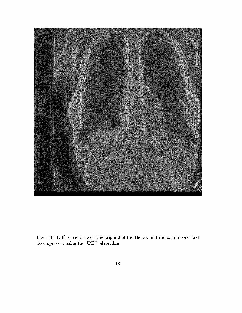
Figure 6: Di�erence between the original of the thorax and the compressed anddecompressed using the JPEG algorithm.16