arX

iv:0

709.

4509

v1 [

mat

h.C

O]

27

Sep

2007

A RECURSION FORMULA FOR k-SCHUR FUNCTIONS

DANIEL BRAVO AND LUC LAPOINTE

Abstract. The Bernstein operators allow to build recursively the Schur functions. We present arecursion formula for k-Schur functions at t = 1 based on combinatorial operators that generalizethe Bernstein operators. The recursion leads immediately to a combinatorial interpretation for theexpansion coefficients of k-Schur functions at t = 1 in terms of homogeneous symmetric functions.

1. Introduction

The study of Macdonald polynomials led to the discovery of symmetric functions, s(k)λ (t), indexed

by partitions whose first part is no larger than a fixed integer k ≥ 1, and depending on a parameter

t. Experimentation suggested that when t = 1, the functions s(k)λ := s

(k)λ (1) play the fundamen-

tal combinatorial role of the Schur basis in the symmetric function subspace Λk = Z[h1, . . . , hk];that is, they satisfy properties generalizing classical properties of Schur functions such as Pieri and

Littlewood-Richardson rules. The study of the s(k)λ led to several characterizations [6, 7, 9] (conjec-

turally equivalent) and to the proof of many of these combinatorial conjectures. We thus generically

call the functions s(k)λ k-Schur functions (at t = 1), but in this article consider only the definition

presented in [9].

The Bernstein operators Bn =∑

i≥0(−1)ihn+i e⊥i (see Section 3 for the relevant definitions) allow

to build the Schur functions recursively. That is, if λ = (λ1, . . . , λℓ) is a partition, we have

Bλ1Bλ2 · · ·Bλℓ= sλ , (1.1)

where sλ is the Schur function indexed by the partition λ.

We present in this article a recursion for k-Schur functions that generalizes this recursion. It isbased on a combinatorial generalization of the Bernstein operators,

B(k)λ1

B(k)λ2· · ·B

(k)λℓ

= s(k)λ , (1.2)

where λ = (λ1, . . . , λℓ) is a partition such that λ1 ≤ k. In this case, the operators B(k)i are only

defined on certain subspaces of Λk, preventing for instance the study of the commutation relationsthat they could have satisfied. The term combinatorial is used to emphasize the fact that the

operators B(k)i are defined through their action on certain k-Schur functions, an action which is

combinatorially much in the spirit of the action of the usual Bi’s on Schur functions.

Formula (1.2) leads immediately to a combinatorial interpretation for the expansion coefficients ofk-Schur functions in terms of homogeneous symmetric functions. This interpretation is particularlyrelevant given that no Jacobi-Trudi type determinantal formula has yet been obtained for k-Schurfunctions.

Key words and phrases. Symmetric functions, Schur functions, Bernstein operators, k-Schur functions.L. L. was partially supported by the Anillo Ecuaciones Asociadas a Reticulados financed by the World Bank

through the Programa Bicentenario de Ciencia y Tecnologıa, NSF grant DMS-0652641, and by the Programa Retic-ulados y Ecuaciones of the Universidad de Talca.

1

It was shown in [4] that the k-Schur functions form the Schubert basis for the homology of theaffine (loop) Grassmannian of GLk+1. This implies that the k-Littlewood-Richardson coefficientscλ,kµν ∈ N appearing in

s(k)µ s(k)

ν =∑

λ

cλ,kµν s

(k)λ (1.3)

are the structure constants for the homology of the affine (loop) Grassmannian of GLk+1. Fur-thermore, these coefficients are known [10] to contain as a subset the Gromow-Witten invariants ofthe quantum cohomology ring of the Grassmannian (or equivalently the fusion rules for the Wess-Zumino-Witten conformal field theories in case A). Finding combinatorial interpretations for thesequantities is still an open problem. Given that the Bernstein operators have been used to derivethe Littlewood-Richardson rule (see [2]), we hope that the recursion formula for k-Schur functionspresented in this article will provide some of the insight needed for finding such combinatorialinterpretations.

2. Definitions

2.1. Basic definitions. Most of the definitions in this subsection are taken from [12]. A partitionλ = (λ1, . . . , λm) is a non-increasing sequence of positive integers. The degree of λ is |λ| = λ1 +· · ·+ λm and the length ℓ(λ) is the number of parts m. Each partition λ has an associated Ferrersdiagram with λi lattice squares in the ith row, from the bottom to top. For example,

λ = (4, 2, 1) = (2.1)

Given a partition λ, its conjugate λ′ is the diagram obtained by reflecting λ about the main diagonal.A partition λ is “k-bounded” if λ1 ≤ k. Any lattice square in the Ferrers diagram is called a cell,where the cell (i, j) is in the ith row and jth column of the diagram. We say that λ ⊆ µ when λi ≤ µi

for all i. The dominance order D on partitions is defined by λDµ when λ1 + · · ·+λi ≥ µ1 + · · ·+µi

for all i, and |λ| = |µ|.

A skew diagram µ/λ, for any partition µ containing the partition λ, is the diagram obtained bydeleting the cells of λ from µ. The thick frames below represent (5,3,2,1)/(4,2).

The degree of a skew diagram µ/λ is |µ| − |λ|. We say that the skew diagram µ/λ of degree ℓ is ahorizontal (resp. vertical) ℓ-strip if it never has two cells in the same column (resp. row).

A cell (i, j) of a partition γ with (i + 1, j + 1) 6∈ γ is called “extremal ”. A “removable” cornerof partition γ is a cell (i, j) ∈ γ with (i, j + 1), (i + 1, j) 6∈ γ and an “addable” corner of γ is asquare (i, j) 6∈ γ with (i, j − 1), (i− 1, j) ∈ γ (note that (1, γ1 + 1), (ℓ(γ) + 1, 1) are also consideredto be addable corners). All removable corners are extremal. In the figure below we have labeled alladdable corners with a, labeled extremal cells e, and framed the removable corners.

a

e e a

e e

e a

e e e a

The hook-length of a cell c = (i, j) in a partition λ is λi− j +λ′j − i+1. That is, the number of cells

in λ to the right of c plus the number of cells in λ above c plus one. If, as above, λ = (5, 3, 3, 2),the hook-length of the cell (1, 2) is 7. We will say that a cell is k-bounded if its hook-length is notlarger than k.

2

Recall that a “k+1-core is a partition that does not contain any k+1-hooks (see [3] for a discussionof cores and residues). An example of a 6-core (with the hook-length of each cell indicated) is:

1

4 2 1

5 3 2

7 5 4 1

The “k + 1-residue” of square (i, j) is j − i mod k + 1. That is, the integer in this square whensquares are periodically labeled with 0, 1, . . . , k, where zeros lie on the main diagonal. Here are the5-residues associated to (6, 4, 3, 1, 1, 1)

0

1

2

3 4 0

4 0 1 2

0 1 2 3 4 0

We will need the following basic result on cores [1, 8].

Proposition 1. Let γ be a k + 1-core.

(1) Let c and c′ be extremal cells of γ with the same k + 1-residue (c′ weakly north-west of c).(a) If c is at the end of its row, then so is c′.(b) If c has a cell above it, then so does c′.

(2) Let c and c′ be extremal cells of γ with the same k + 1-residue (c′ weakly south-east of c).(a) If c is at the top of its column, then so is c′.(b) If c has a cell to its right, then so does c′.

(3) A k + 1-core γ never has both a removable corner and an addable corner of the same k + 1-residue.

2.2. Bijection: k + 1-cores and k-bounded partitions. Let Ck+1 and Pk respectively denotethe collections of k +1 cores and k-bounded partitions. There is a bijective correspondence betweenk + 1-cores and k-bounded partitions that was defined in [8] by the map:

p : Ck+1 → Pk where p (γ) = (λ1, . . . , λℓ) ,

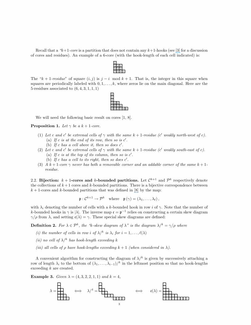
with λi denoting the number of cells with a k-bounded hook in row i of γ. Note that the number ofk-bounded hooks in γ is |λ|. The inverse map c = p−1 relies on constructing a certain skew diagramγ/ρ from λ, and setting c(λ) = γ. These special skew diagrams are defined:

Definition 2. For λ ∈ Pk, the “k-skew diagram of λ” is the diagram λ/k = γ/ρ where

(i) the number of cells in row i of λ/k is λi for i = 1, . . . , ℓ(λ)

(ii) no cell of λ/k has hook-length exceeding k

(iii) all cells of ρ have hook-lengths exceeding k + 1 (when considered in λ).

A convenient algorithm for constructing the diagram of λ/k is given by successively attaching arow of length λi to the bottom of (λ1, . . . , λi−1)/

k in the leftmost position so that no hook-lengthsexceeding k are created.

Example 3. Given λ = (4, 3, 2, 2, 1, 1) and k = 4,

λ = ⇐⇒ λ/4 = ⇐⇒ c(λ) =

3

2.3. Affine symmetric group. The affine symmetric group Sk+1 is generated by the k+1 elementsσ0, . . . , σk satisfying the affine Coxeter relations:

σ2i = id, σiσj = σjσi (i− j 6= ±1 mod k + 1), and σiσi+1σi = σi+1σiσi+1 . (2.2)

Here, and in what follows, σi is understood as σi modk+1 if i ≥ k + 1. Elements of Sk+1 are called

affine permutations, or simply permutations. The length of an element σ ∈ Sk+1 is the smallestnumber ℓ such that σ can be written as σ = σi1 · · ·σiℓ

for some i1, . . . , iℓ ∈ {0, 1, . . . , k}.

Let Sk+1 be the subgroup of Sk+1 generated by σ1, . . . , σk (and thus isomorphic to the usualsymmetric group on k elements). It is known that the minimal length (left) coset representatives in

the quotient Sk+1/Sk+1 are in bijective correspondence with k + 1-cores (and thus with k-boundedpartitions). There is a natural action of the affine symmetric group on cores that accounts for thisrelation [13, 11]:

Definition 4. The “operator σi” acts on a k + 1-core by:

(a) removing all removable corners with k +1-residue i if there is at least one removable cornerof k + 1-residue i

(b) adding all addable corners with k + 1-residue i if there is at least one addable corner withk + 1-residue i

In that correspondence, if σ = σi1 · · ·σiℓis a minimal length coset representative in Sk+1/Sk+1,

then σi1 · · ·σiℓ(∅) is the corresponding core (where ∅ is the empty core). Given this correspondence,

in what follows we will not distinguish between cores and minimal length coset representatives inSk+1/Sk+1. We will also write σ ∈ Sk+1/Sk+1 to mean that σ ∈ Sk+1 is a minimal length cosetrepresentative. Note that σi is not defined when there are no addable or removable corners ofresidue i. In this case, the corresponding permutation is not a minimal length coset representativein Sk+1/Sk+1, and will thus be of no concern to us.

Example 5. Given k = 3, the product σ2σ3σ1σ0 ∈ S4/S4 corresponds to the 4-core γ = (3, 1, 1),since:

σ2σ3σ1σ0(∅) = σ2σ3σ1 ( 0 ) = σ2σ3 ( 0 1 ) = σ2

(

3

0 1

)

=2

3

0 1 2

Given r < s ∈ Z, we can define the transposition tr,s ∈ Sk+1 by

tr,s = σrσr+1 · · ·σs−2σs−1σs−2 · · ·σr+1σr (2.3)

It is easy to see that tr,s is an involution. Furthermore, if s− r < k + 1, then it is easy to see usingthe Coxeter relations that

tr,s = σs−1σs−2 · · ·σr+1σrσr+1 · · ·σs−2σs−1 . (2.4)

Now, given two k + 1-cores δ and γ, we say that δ ⋖ γ if there exists a transposition tr,s such that

tr,sδ = γ and |p(γ)| = |p(δ)| + 1. The transitive closure of this relation corresponds in Sk+1/Sk+1

to the (strong) Bruhat order.

Example 6. Let k = 3 and λ = (2, 1, 1). Apply t1,3 to c(λ) = (3, 1, 1) = γ.

t1,3(γ) = σ1σ2σ1

(

2

3

0 1 2

)

= σ1σ2

(

1

2

3

0 1 2

)

= σ1

(

1

2

3

0 1

)

=2

3

0

= δ

Also note that t1,3(δ) = γ. Since p(δ) = (1, 1, 1), then we have that (1, 1, 1) ⋖ (3, 1, 1).

Equivalently, it can be shown that δ ⋖ γ iff δ ⊂ γ and |p(γ)| = |p(δ)|+1. It is also known [13, 11]that the Bruhat order, the transitive closure of this relation, is given by δ < γ iff δ ⊂ γ.

The following result is proved in [5]. Note that a ribbon is a connected skew-diagram that doesnot contain any (2, 2) subdiagram.

4

Proposition 7. Let δ ⋖ γ be k + 1-cores with tr,sδ = γ and 0 < r < s. Then

(1) s− r < k + 1.(2) Each connected component of γ/δ is a ribbon with s− r cells in diagonals of k + 1-residues

r, r + 1, . . . , s− 1.(3) The components are translates of each other and their heads lie on “consecutive” diagonals

of k + 1-residue s− 1.

2.4. k-Schur functions. We now present the characterization of k-Schur functions given in [9].

Definition 8. Let γ be a k+1-core with m k-bounded hooks and let α = (α1, . . . , αr) be a compositionof m. A “k-tableau” of shape γ and “k-weight” α is a filling of γ with integers 1, 2, . . . , r such that

(i) rows are weakly increasing and columns are strictly increasing

(ii) the collection of cells filled with letter i are labeled by exactly αi distinct k + 1-residues.

Example 9. The 3-tableaux of 3-weight (1, 3, 1, 2, 1, 1) and shape (8, 5, 2, 1) are:

5

4 6

2 3 4 4 6

1 2 2 2 3 4 4 6

6

4 5

2 3 4 4 5

1 2 2 2 3 4 4 5

4

3 6

2 4 4 5 6

1 2 2 2 4 4 5 6

Remark 10. When k is large, a k-tableau T of shape γ and k-weight µ is a semi-standard tableauof weight µ since no two diagonals of T will have the same residue.

We denote the set of all k-tableaux of shape c(µ) and k-weight α by T kα (µ), and define the

“k-Kostka numbers” as:

K(k)µα = |T k

α(µ)| . (2.5)

As is the case for the Kostka number, they are such that K(k)µα = K

(k)µγ if γ is a permutation of α,

and satisfy a triangularity property.

Property 11. For any k-bounded partitions λ and µ,

K(k)µλ = 0 when µ 4 λ and K(k)

µµ = 1 . (2.6)

Thus the matrix ||K(k)||µ,λ (with µ and λ running over all k-bounded partitions of a given degree)is invertible, naturally giving rise to a family of symmetric functions.

Definition 12. The “k-Schur functions”, indexed by k-bounded partitions, are defined as formingthe unique basis of Λk = Z[h1, . . . , hk] such that:

hλ = s(k)λ +

∑

µ:µ⊲λ

K(k)µλ s(k)

µ for all λ such that λ1 ≤ k . (2.7)

From this k-tableau characterization, many properties of k-Schur functions are derived in [9]. Ofthese properties, the only one relevant to this work is the k-Pieri rule, which we now present in theform given in [5].

Any proper subset A ( Zk+1 = {0, . . . , k} decomposes into unions I1 ∪ I2 ∪ · · · ∪ Im of maximalcyclic intervals. For each cyclic component [a, b] of A, we will let σA be equal to the productof factors σbσb−1 · · ·σa (observe the descending order of the indices). For instance, if k = 8 andA = {0, 1, 3, 4, 6, 8}, we have that the cyclic components are [8, 1] = {8, 0, 1}, [3, 4] = {3, 4} and[6, 6] = {6}. The corresponding element σA is thus equal to σ1σ0σ8σ4σ3σ6 = σ4σ3σ6σ1σ0σ8 = · · ·(the components commute among themselves).

5

Proposition 13. Let hℓ be the ℓth complete symmetric function. Furthermore, let λ be a k-boundedpartition, and γ = c(λ) be its corresponding k +1-core. Then, if ℓ ≤ k, the k-Schur functions satisfythe k-Pieri rule:

hℓ s(k)λ =

∑

A

s(k)p(σA(γ)) (2.8)

where the sum is over all subsets A of Zk+1 of cardinality ℓ such that p(σA(γ)) is a partition of sizeℓ + |λ|.

Remark 14. This formulation of the k-Pieri rule is equivalent to the one presented in [9]. In thatcase, the k-Pieri rule can be interpreted as

hℓ s(k)λ =

∑

µ

s(k)µ , (2.9)

where the sum is over all k-bounded partitions µ such that c(µ)/c(λ) is a horizontal strip with exactlyℓ = |µ| − |λ| distinct residues. In [5], it is shown that this condition is equivalent to c(µ) being equalto σA(c(λ)) for A a subset of Zk+1 of cardinality ℓ.

Example 15. We illustrate the k-Pieri rule for k = 6 by doing the product of h4 and s(6)(4,3,2,2,2,1).

First, we give the Ferrers diagram of the k + 1-core c(λ) associated to λ = (4, 3, 2, 2, 2, 1), withresidues on the addable positions and frames on the k-bounded cells.

1

3

0 1

3 4

6 0 1 2

We then show the possible subsets A of Zk+1 of cardinality ℓ = 4 such that that p(σA(c(λ))) is apartition of 18:

1

3

0 1

3 4

6 0 1 2

1

3

0 1

3 4

6 0 1 2

1

3

0 1

3 4

6 0 1 2

{6, 0, 1, 2} {6, 0, 1, 3} {6, 0, 3, 4}

1

3

0 1

3 4

6 0 1 2

1

3

0 1

3 4

6 0 1 2

{6, 1, 3, 4} {0, 1, 3, 4}

Therefore,

h4s(6)(4,3,2,2,2,1) = s

(6)(6,3,3,2,2,1,1) + s

(6)(5,3,3,2,2,2,1) + s

(6)(5,4,3,2,2,2) + s

(6)(5,4,2,2,2,2,1) + s

(6)(4,4,3,2,2,2,1) (2.10)

3. Bernstein operators

The notation used in this section is taken from [12]. For m a nonnegative integer, the operatore⊥m is defined such that given any symmetric functions f and g,

〈e⊥m f, g〉 = 〈f, em g〉 , (3.1)

with em the mth elementary symmetric function and 〈·, ·〉 the unique scalar product with respect towhich the Schur functions are orthonormal. It can be shown that the operator e⊥m has the followingsimple action on a Schur function

e⊥m sλ =∑

µ

sµ (3.2)

6

where the sum is over all partition µ such that λ/µ is a m-vertical strip.

For n a nonnegative integer, the Bernstein operator is [14]

Bn =∑

i≥0

(−1)ihn+i e⊥i , (3.3)

where hm is the mth complete symmetric function. The Bernstein operators allow to build the Schurfunctions recursively. That is, for λ = (λ1, . . . , λℓ),

Bλ1Bλ2 · · ·Bλℓ· 1 = sλ . (3.4)

Or equivalently, if λ = (λ2, . . . , λℓ), then

Bλ1 sλ = sλ . (3.5)

4. The main formula

Note that for the remainder of the article, as it was the case in the previous section, λ will standfor the partition λ without its first part.

Before being able to describe analogs of these operators for the k-Schur functions, we need somedefinitions. Let γ be a k +1-core, and let x be the cell corresponding to the leftmost k-bounded cellin the first row of γ. If x lies in column j, then let the main subpartition of γ (relatively to γ), bethe subpartition of γ made out of the columns of γ from column j up to column γ2 (that is, fromcolumn j rightward). For instance, let k = 6, and consider the 7-core γ = (5, 5, 3, 3, 2, 2, 1, 1, 1). Asillustrated in the following diagram, where the k-bounded cells of γ are in bold face, the leftmostk-bounded cell, x, in the first row of γ is in column 3. Therefore, the main subpartition of γ is thepartition filled with ◦’s in the diagram.

x

=⇒◦

◦

◦ ◦ ◦

Remark 16. It is important to realize that the concept of main subpartition is only defined for aδ such that δ = ω for a given k + 1-core ω. When using the term main subpartition of γ, it isunderstood that the larger partition is in this case γ.

Remark 17. The cells in the main subpartition of γ are all k-bounded. When k is large enough,the main subpartition of γ coincides with γ.

Remark 18. If in γ there are columns to the left of its main subpartition, then they are all strictlylarger than the largest column of the main subpartition. This is because the cell to the left of x in γ(see the example above) would not have otherwise a hook-length larger than k + 1.

Recall that δ ⋖ ω iff δ ⊆ ω and the number of k-bounded hooks in δ is one less than that in ω.Also recall from Proposition 7 that if δ ⋖ ω, then ω/δ is a union of identical ribbons (of size smalleror equal to k) whose heads (southeast-most cell of the ribbon) occur on consecutive diagonals ofa certain k + 1-residue. A ribbon will be horizontal if, as its name suggests, it coincides with ahorizontal partition (n) for some n.

Definition 19. Let γ be a core such that the main subpartition of γ is of length m. We will saythat the core δ can be obtained by removing a vertical (k, ℓ)-strip from γ if there exists a sequenceof cores γ = ω(1) ⊃ ω(2) ⊃ · · · ⊃ ω(ℓ+1) = δ such that

(1) ω(i+1) ⋖ ω(i) for all i = 1, . . . , ℓ.7

(2) ω(i)/ω(i+1) is a union of horizontal ribbons, the lowest of which appears in a row ri with1 ≤ ri ≤ m.

(3) r1, . . . , rℓ are all distinct.

Example 20. Let k = 5 and consider γ = (6, 6, 3, 3, 3, 1, 1, 1, 1). It can be checked that the lengthof the main subpartition of γ is m = 2. The k + 1-core δ = (5, 4, 3, 2, 1, 1, 1, 1, 1) can be obtainedfrom γ, by removing the following vertical (5, 2)-strip :

γ = ω(1) = (6, 6, 3, 3, 3, 1, 1, 1, 1)⊃ ω(2) = (6, 4, 3, 3, 1, 1, 1, 1, 1)⊃ ω(3) = (5, 4, 3, 2, 1, 1, 1, 1, 1) = δ.

In the following sequence of Ferrers diagrams, we see that all the conditions for a a vertical (5, 2)-strip are satisfied. The framed cells correspond to successive ribbons having their lowest occurrencein different rows and within the first m = 2 rows.

⊃ ⊃

Remark 21. By Remark 18, in condition (2) of Definition 19, the lowest ribbons are always con-tained entirely in the main subpartition of γ.

Lemma 22. Suppose we have a vertical (k, ℓ)-strip γ = ω(1) ⊃ ω(2) ⊃ · · · ⊃ ω(ℓ+1) = δ, whose lowestribbons occur in rows r1, . . . , rℓ. Then, there exists a sequence γ = ω(1) ⊃ ω(2) ⊃ · · · ⊃ ω(ℓ+1) = δ,whose lowest ribbons occur in rows r1 > · · · > rℓ. That is, removing a vertical (k, ℓ) strip can alwaysbe done in a certain order (by removing the ribbon whose lowest ribbon is the highest, then the onewhose lowest ribbon is the second highest, and so on).

Proof. Suppose we have ω(i+1) ⋖ ω(i) ⋖ ω(i−1), with both ω(i−1)/ω(i) and ω(i)/ω(i+1) given by aunion of horizontal ribbons, the lowest of which are respectively R1 and R2. By Proposition 7, wehave ω(i) = tr,s(ω

(i−1)), where r (resp. s − 1) is the residue of the leftmost (resp. rightmost) cell

in R1. Similarly, we have ω(i+1) = tr′,s′(ω(i)), where r′ (resp. s′ − 1) is the residue of the leftmost(resp. rightmost) cell in R2. If R1 does not sit on top of R2 (in which case R1 would necessarilyhave to be removed first), we have that the cyclic intervals [r, s− 1] and [r′, s′ − 1] are disjoint andnot contiguous. This is because R1 and R2 belong to the main subpartition of γ (which does nothave repeated diagonals of the same residue) and because r 6= s′ mod k +1 (otherwise there wouldbe a hook of length k + 1 in the core ω(i−1)). Observe that in this case,

tr′,s′tr,s(ω(i−1)) = tr,s

(

tr′,s′(ω(i−1)))

⋖ tr,s(ω(i−1)) =⇒ tr′,s′(ω(i−1)) ⋖ ω(i−1)

and

tr,s(ω(i−1)) ⋖ ω(i−1) =⇒ tr′,s′tr,s(ω

(i−1)) = tr′,s′

(

tr,s(ω(i−1))

)

⋖ tr′,s′(ω(i−1)) ,

since there is no interference in the adding and deleting process involved in acting with the trans-positions. Therefore,

ω(i+1) = tr′,s′tr,s(ω(i−1)) ⋖ tr,s(ω

(i−1)) ⋖ ω(i−1)

leads to

ω(i+1) = tr′,s′tr,s(ω(i−1)) ⋖ tr′,s′(ω(i−1)) ⋖ ω(i−1) ,

meaning that the ribbons R1 and R2 (with their translates) can be removed in any order. Thegeneral result then follows by applying this idea again and again. �

The following results will show that removing a (k, ℓ)-strip from a k+1-core γ removes a ℓ-verticalstrip from the k-bounded partition associated to γ.

8

Lemma 23. Let γ and δ be two k + 1-cores such that |p(γ)| = |p(δ)| + 1 and such that δ ⊂ γ. Ifγ/δ is a union of horizontal ribbons, the highest of which appears in row i, then p(γ) = p(δ) + ei,where ei is the vector with a 1 in position i and 0 everywhere else.

Proof. First note that if a row of γ/δ does not contain a horizontal ribbon then the number ofk-bounded cells in that row is the same in γ and in δ. This is because the hook-length of a cell inthat row is changed by at most one cell, preventing a change of the hook length from more thank + 1 to less than k + 1 (recall that a k + 1-core does not contain cells with hook-lengths of k + 1).As for the remaining rows, recall that the head of the ribbons occur in consecutive diagonals of thesame residues. The proof is then illustrated in the following example at k = 3, where the cells inbold face are the horizontal ribbons in γ/δ, and the cells with an x are the cells that went from notbeing k-bounded in γ to being k-bounded in δ.

x

x x

x x

One simply needs to observe that in each row that contains a ribbon, the number of cells with an xis equal to the number of cells in bold face (except in the highest such row). Since |p(γ)| = |p(δ)|+1,this implies that it must differ by one in the highest row that contains a ribbon. �

Proposition 24. Let δ and γ be k + 1-cores such that δ can be obtained by removing a vertical(k, ℓ)-strip from γ. Then p(γ)/p(δ) is a vertical ℓ-strip (in the usual sense).

Proof. From the previous lemma, we simply need to show that when going from γ to δ by removinghorizontal ribbons, two ribbons will never occur in the same row. From Lemma 22, it is possible tochoose γ = ω(1) ⊃ ω(2) ⊃ · · · ⊃ ω(ℓ+1) = δ such that the horizontal ribbons are removed from topto bottom in the main subpartition. Let ω(i)/ω(i+1) contain a given ribbon R and all its translates.

The rightmost cell of R, the translate of R in the main subpartition, has a residue r that is notcontained in any ribbon above it in the main subpartition (from Remark 21 and 17). Therefore,when going from γ to ω(i), no cells of residue r are removed or added, and thus the rightmost cellof R is also extremal in γ. By Proposition 1, this means that the rightmost cell of R has to beat the end of its row in γ since the rightmost cell of R is also at the end it its row in γ (no tworibbons can occur in the same row of the main subpartition by definition of (k, ℓ)-strip). Therefore,

no horizontal ribbons can ever occur to the right of R. �

We can now define the recursion for k-Schur functions that extends formula (3.5).

Definition 25. Let V(k,r) be the Z-linear span of k-Schur functions whose first part is not larger

than r. Given a partition ν such that s(k)ν ∈ V(k,r), let λ = (r, ν1, ν2, . . . ) and γ = c(λ). Then the

linear operator e⊥ℓ,r is defined on V(k,r) to be such that

e⊥ℓ,r s(k)ν =

∑

µ

s(k)µ , (4.1)

where the sum is over all k-bounded partition µ such that c(µ) can be obtained by removing a vertical(k, ℓ)-strip from γ. If there is no such µ, the result is simply defined to be zero.

Note that we only use the symbol e⊥ℓ,r in analogy with e⊥ℓ . That is, to the best of our knowledge,

e⊥ℓ,r is not the adjoint of multiplying by some symmetric function eℓ,r with respect to any scalar

product. We should also point out that the operator e⊥ℓ,r does in fact depends on r, since r appears

in the definition of the k + 1-core γ (and since extracting a (k, ℓ)-strip from γ actually depends onγ).

9

Remark 26. By Proposition 24, the µ’s such that s(k)µ occur in in the action of e⊥ℓ,r on s

(k)ν are

such that ν/µ is a vertical ℓ-strip. These µ’s are thus a subset of the µ’s such that sµ occur in theaction of e⊥ℓ on sν .

Example 27. Let ν = (4, 3, 2, 2, 1) and k = 6. Then λ = (4, 4, 3, 2, 2, 1) and γ = c(λ) =(6, 6, 3, 2, 2, 1). Hence

γ = (6, 3, 2, 2, 1) =

where the framed cells correspond to the main subpartition. If we apply e⊥1,4, the vertical (k, ℓ)-stripsneed to be of length ℓ = 1. The following diagrams show the vertical (k, 1)-strips that can be obtained,with the k-bounded cells marked with ◦ (thus corresponding to the k-bounded partitions).

⊃

◦

◦

◦ ◦

◦ ◦ ◦

◦ ◦ ◦ ◦

⊃

◦

◦ ◦

◦ ◦

◦ ◦

◦ ◦ ◦ ◦

⊃

◦

◦ ◦

◦ ◦

◦ ◦ ◦

◦ ◦ ◦

From here, we obtain that

e⊥1,4 s(6)ν = s

(6)(4,3,2,1,1) + s

(6)(4,2,2,2,1) + s

(6)(3,3,2,2,1) . (4.2)

Now, for r = 1, . . . , k, let

B(k)r =

∑

ℓ≥0

(−1)ℓhr+ℓ e⊥ℓ,r . (4.3)

Note that this operator is only defined on V(k,r). The main result of this article is then the following.

Theorem 28. Let λ = (λ1, λ2, . . . ) be a k-bounded partition. Then

B(k)λ1

s(k)

λ= s

(k)λ . (4.4)

Example 29. Using k and λ as in Example 27, we will show that:

B(6)4 s

(6)

λ= s

(6)λ . (4.5)

By definition, our equation amounts to:

B(6)4 s

(6)

λ=∑

ℓ≥0

(−1)ℓh4+ℓ e⊥ℓ,4s(6)

λ. (4.6)

According to the diagram of equation (27), we only need to consider vertical (k, ℓ)-strips up to ℓ = 2.

For the first term in the sum, acting with e⊥0,4 on s(6)

λgives s

(6)

λ, since we have to extract a vertical

(k, 0)-strip (which amounts to doing nothing). The action of e⊥1,4 was explained in example 27. To

compute the action of e⊥2,4 on s(6)

λ, we present here the diagrams of the cores that can be obtained by

removing a vertical (k, 2)-strips from λ:

⊃ ⊃

◦

◦

◦ ◦

◦ ◦

◦ ◦ ◦ ◦

10

⊃ ⊃

◦

◦ ◦

◦ ◦

◦ ◦

◦ ◦ ◦

Therefore, (4.6) gives:

B(6)4 s

(6)

λ= h4(s

(6)

λ)− h5(s

(6)(4,3,2,1,1) + s

(6)(4,2,2,2,1) + s

(6)(3,3,2,2,1)) + h6(s

(6)(4,2,2,1,1) + s

(6)(3,2,2,2,1)) (4.7)

Now, by applying the k-Pieri rule we get:

B(6)4 s

(6)

λ= s

(6)4,4,3,2,2,1 + s

(6)5,4,3,2,1,1 + s

(6)6,3,3,2,1,1 + s

(6)5,3,3,2,2,1 + s

(6)6,3,3,2,2 + s

(6)5,4,2,2,2,1

−s(6)6,3,3,2,1,1 − s

(6)5,4,3,2,1,1 − s

(6)6,3,2,2,2,1 − s

(6)5,4,2,2,2,1 − s

(6)6,4,2,2,1,1 − s

(6)6,3,3,2,2 − s

(6)5,3,3,2,2,1

+s(6)6,4,2,2,1,1 + s

(6)6,3,2,2,2,1.

Finally, canceling the expression gives B(6)4 s

(6)

λ= s

(6)4,4,3,2,2,1 = s

(6)λ .

The proof of the theorem will be of a combinatorial nature, and will ultimately rely on theconstruction of a sign-reversing involution. But first, we introduce some notation.

Definition 30. Given γ = c(λ), let D(k)λ be the set of pairs (δ, A) such that for some ℓ = 0, . . . , k−λ1:

(1) γ/δ is a removable vertical (k, ℓ)-strip(2) A is a subset of Zk+1 of cardinality λ1 + ℓ such that σA(δ) satisfies |p(σA(δ))| = |λ| (that

is, σA(δ) is a k + 1-core whose number of k-bounded cells is |λ|).

A pair (δ, A) ∈ D(k)λ can be thought of as the Ferrer’s diagram of γ with the cells of γ/δ marked

with an O combined with the cells of σA(δ)/δ marked with an X . We will refer to such a diagramas the OX diagram associated to the pair (δ, A). Observe by Remark 14 that an OX diagram cannever have two X ’s in the same column since σA(δ)/δ is a horizontal strip. Cells that contain a Oand an X will be called OX cells and represented by XO in diagrams.

Example 31. In example 29, when we expand the products, we see that the k-Schur function

s(6)(6,3,2,2,1) appears two times, first in the product h5s

(6)(4,2,2,2,1) and then in the product h6s

(6)(3,2,2,2,1). If

we consider the (δ, A) pairs and their corresponding OX diagrams associated to these two occurrences

of s(6)(6,3,2,2,1), we see that the first one is:

((6, 2, 2, 2, 1), {4, 6, 0, 1, 2}) ←→

X

X

XO X

XXXX

while the second one is:

((4, 2, 2, 2, 1), {4, 5, 6, 0, 1, 2}) ←→

X

X

XO X

XO XO XXXX

Definition 32. Let (δ, A) ∈ D(k)λ , and let γ = c(λ). A changeable cell of the pair (δ, A) is a cell of

the core σA(δ) that i) lies at the top of its column and ii) belongs to γ. The set of pairs (δ, A) ∈ D(k)λ

such that (δ, A) has a changeable cell will be denoted C(k)λ .

Remark 33. In the language of the OX diagram associated to (δ, A), a changeable cell is a cell ofσA(δ) at the top of its column that is either empty or filled with an OX.

Example 34. In example 31, the changeable cells of the two OX diagrams are located in the samepositions: in the fifth and sixth cells of the first row and in the third cell of the second row.

11

Proof of Theorem 28. Equation (4.4) can be rewritten as∑

ℓ≥0

(−1)ℓhλ1+ℓ e⊥ℓ,λ1s(k)

λ= s

(k)λ . (4.8)

Using the action of hλ1+ℓ and e⊥ℓ,λ1on k-Schur functions, this is equivalent to∑

(δ,A)∈D(k)λ

(−1)|A|−λ1s(k)p(σA(δ)) = s

(k)λ . (4.9)

Let γ = c(λ). We will show in Lemma 37 that the pair (γ, B), where B is the subset of Zk+1 of size

λ1 such that σB(γ) = γ, is the unique pair of D(k)λ that does not have a changeable cell. Given that

the pair (γ, B) corresponds to a term +s(k)λ in the l.h.s. of (4.9), to prove Theorem 28 is suffices to

show that∑

(δ,A)∈C(k)λ

(−1)|A|s(k)p(σA(δ)) = 0 , (4.10)

where we recall that C(k)λ is the set of (δ, A) ∈ D

(k)λ that have a changeable cell.

This result will readily follow if there exists an involution ϕ : C(k)λ → C

(k)λ that maps the pair

(δ, A) to a pair (δ′, A′) such that σA(δ) = σA′(δ′) and (−1)|A| = −(−1)|A′|. Such a sign-reversing

involution will be constructed in the next section (see Definition 41 and Proposition 46). �

By applying Theorem 28 again and again, we obtain a combinatorial interpretation for the ex-pansion coefficients of k-Schur functions in terms of homogeneous symmetric functions.

Corollary 35. Let λ be a k-bounded partition such that c(λ) = γ. Suppose that the sequence S =(γ(0), . . . , γ(r)), with ∅ = γ(0) ( γ(1) ( · · · ( γ(r) = γ, is such that for all i = 1, . . . , r, we have thatγ(i−1) can be obtained by removing a (k, ℓi)-vertical strip from γ(i) for some ℓi ∈ {0, . . . , k}. Definepart(S) to be the partition corresponding to the rearrangement of the sequence (ℓ1 + p1, . . . , ℓr + pr),where pi is the length of the first row of p(γ(i)) (equivalently, pi is the number of k-bounded cells inthe first row of γ(i)). Finally, define sgn(S) to be (−1)ℓ1+···+ℓr . Then

s(k)λ =

∑

S

sgn(S)hpart(S) , (4.11)

where the sum is over all possible sequences S of the form given above.

Example 36. The sequences S in the previous corollary can be interpreted as certain fillings ofγ = c(λ), as we will illustrate with an example. If k = 4 and λ = (2, 2, 2, 1), the possible sequencesS are seen to be in correspondence with the following fillings of γ = (3, 2, 2, 1):

1

2 2

3 3

4 4 4

1

1 1

2 2

3 3 3

2

1 1

2 2

3 3 3

1

2 3

3 3

4 4 4

1

1 2

2 2

3 3 3

2

1 2

2 2

3 3 3

1

2 4

3 3

4 4 4

1

1 3

2 2

3 3 3

2

1 3

2 2

3 3 3

1

1 2

1 1

2 2 2

1

2 4

3 4

4 4 4

1

1 3

2 3

3 3 3

2

1 3

2 3

3 3 3

1

1 2

1 2

2 2 2

In these diagrams, the partition γ(i) for a sequence S = (γ(0), . . . , γ(r)) can be obtained by readingthe subdiagram containing the letters up to i in the diagram. The framed cells containing letter iindicate the location of the (k, ℓi)-vertical strip extracted from γ(i) to obtain γ(i−1). For instance,the fifth diagram of the second row, corresponds to the sequence S′ = (∅, (1, 1), (1, 1, 1), (3, 2, 2, 1)).We illustrate this with the following figure:

∅1←− 1

1

0←−

1

1

2

2←−

1

1 3

2 3

3 3 3

12

Each diagram corresponds to a k+1-core in the sequence, and the number above each arrow indicatesthe size of the (k, ℓ)-vertical strip that is extracted to obtain the k + 1-core that follows in thesequence. The bold face numbers in each diagram correspond to the k-bounded cells in each firstrow. We then see that part(S′) = (4, 2, 1), coming from the composition (1 + 1, 1 + 0, 2 + 2), andsgn(S′) = (−1)1+0+2 = −1.

We thus have

s(4)(2,2,2,1) = h2h2h2h1 − h3h2h2 − h3h2h2 − h3h2h1h1 + h3h2h2 + h4h2h1 − h3h2h1h1

+h3h2h2 + h3h3h1 − h4h3 + h4h1h1h1 − h4h2h1 − h4h2h1 + h4h3

= h2h2h2h1 − 2h3h2h1h1 + h3h3h1 + h4h1h1h1 − h4h2h1

5. The involution

Lemma 37. The only pair in D(k)λ whose corresponding diagram does not have a changeable cell is

(γ, B), where B is the unique subset of Zk+1 of size λ1 such that σB(γ) = γ.

Proof. It was proven in [9] that the k-Schur functions obey

hℓs(k)ν = s

(k)(ℓ,ν) +

∑

µ

s(k)µ (5.1)

where the sum is over some µ’s that are larger than (ℓ, ν) in dominance order. That there exists aunique subset B of Zk+1 of size λ1 such that σB(γ) = γ follows from that equation when translatedin the language of cores (see the k-Pieri rule (2.8)). By the construction of the core associated toa k-bounded partition (see Example 3), σB(γ) = γ corresponds to γ with cells added in all thecolumns of γ plus possibly some extra columns. Therefore, the OX diagram of (γ, B) has an X atthe top of every column of σB(γ) = γ. Since there are no O cells (no cells were removed), there areno OX cells and thus there are no changeable cells.

The main observation in the previous paragraph is that acting with σB adds a cell on top of everycolumn of γ. If |A| = |B| and A adds a cell on top of every column of γ, then it is easy to see thatwe must have A = B. This is because in this case, starting from the second row, the cores σA(γ)and σB(γ) are equal since σA(γ)/γ and σB(γ)/γ are horizontal strips. To have the same number ofk-bounded cells, σA(γ) and σB(γ) must thus be equal, which gives that A = B. Therefore, if A 6= Band |A| = |B|, when acting with σA on γ, some columns of γ will not contain an X , and thus somechangeable cells will be present.

If δ 6= γ, then the OX diagram of (δ, A) will contain some O cells. The only possible case withoutchangeable cells is the case where, weakly to the right of a certain column c, the columns are entirelyfilled with O cells (since a cell below an O cell is changeable, as is an OX cell), and where X cellsappear on top of every column of γ to the left of column c.

OO

O

O

O

O O O

X X X

X X

X

X

But this is impossible: from the previous paragraph there are at most |B| distinct residues in thecolumns above γ, and we have to add |A| > |B| residues in a subset of those columns. �

13

Remark 38. The elements of B are the residues of the X’s that sit on top of the main subpartitionof γ plus the residues of the X’s to the right of the main subpartition. This is because by definitionof the main subpartition of γ, the λ1 k-bounded cells in the first row of γ start exactly in the leftmostcolumn of the main subpartition. There are thus exactly λ1 = |B| distinct residues at the top of thecolumns of γ starting from the leftmost column of the main subpartition.

Example 39. Let k = 6, λ = (4, 4, 3, 3, 2, 1, 1) and γ = c(λ). The following Ferrers diagramsillustrate Remark 38. The first is the Ferrers diagram of γ, where the k-bounded cells are given withtheir residues. The second is the OX diagram of the unique pair (γ, B) that has no changeable cells,with the main subpartition in framed cells:

γ =

1

2

3 4

4 5 6

6 0 1

1 2 3 4

3 4 5 6

(γ, B) =

X

X

X

X

XX

X

In this case, B = {1, 3, 4, 6}, recovered from the bold faced X in the second diagram.

Lemma 40. Let (δ, A) ∈ C(k)λ . Then, in the OX diagram associated to (δ, A), there are no O cells

to the right of the rightmost changeable cell in (δ, A). Furthermore, the rightmost changeable cell in(δ, A) is in the main subpartition of γ.

Proof. Let c be the rightmost changeable cell in (δ, A). By definition of a changeable cell, to theright of c in the OX diagram of (δ, A), every column either does not contain any O and finisheswith an X or is entirely made out of O’s. Also observe that, to the right of c, no X cells can appearto the right of an O cell.

Suppose there are some O cells to the right of c. We have in this case δ ⊂ γ. From the previouscomment, the last column of δ is entirely made out of O’s. Now, since σA(δ)/δ is a horizontal stripand, as we have seen in the proof of Lemma 37, γ/γ has a cell over all columns of γ, we have thatσA(δ) ⊂ γ (no X cells can appear to the right of an O cell, and thus no X cell will appear in thecolumns to the right of δ ⊂ γ). But this implies that σA(δ) < γ in the Bruhat order, and thus|p(σA(δ))| < |p(γ)| which is a contradiction. This gives the first claim.

In the case where there are some O cells, by the definition of the pair (δ, A) there are some Ocells in the main subpartition of γ, and thus the first claim immediately implies that the rightmostchangeable cell in (δ, A) is in the main subpartition of γ.

Finally, in the case where there are no O cells, we have δ = γ, |A| = |B|, and A 6= B, with B asin Lemma 37. Suppose that c is not in the main subpartition of γ. Then, in the OX diagram of(γ, A) there are X ’s sitting on top of all columns of the main subpartition. Since, by the argumentabout the Bruhat order given before in the proof, we must have σA(γ) 6⊆ σB(γ) = γ, and since γ/γhas a cell over every column of γ, this implies that the first row of σA(γ) is larger than the first rowof γ. By Remark 38, all the residues in B are thus contained in A. Since |A| = |B|, this gives thecontradiction A = B. �

We now describe the involution ϕ (which will only be shown to be an involution in Proposition 46).

Definition 41. Let (δ, A) ∈ C(k)λ . The involution ϕ is defined according to the two following cases:

I Suppose the rightmost changeable cell c in the OX diagram of (δ, A) is an OX cell, and leti be the row in which it is found. In this case, the cells with an OX in row i are the onlyones with an O. They correspond to a horizontal ribbon R. The involution ϕ then changesthe cells where R and its translates are located into empty cells. This can be translated inthe (δ, A) language in the following way. Let r be the residue of c and let r′ be the residueof the leftmost OX cell in row i. The involution is then ϕ : (δ, A) 7→ (tr′,r+1(δ), A\{r}).

14

II Suppose the rightmost changeable cell c in the OX diagram of (δ, A) is an empty cell, andlet i be the row in which it is found. In this case, it can be shown that c has a residue r thatdoes not belong to A. Let b be the leftmost changeable cell in row i whose residue r′ is suchthat {r′, r′ + 1, . . . , r − 1, r} ⊆ A ∪ {r}. The involution changes the cells in row i from b toc into OX cells (plus the corresponding translates). In the (δ, A) language, this means thatϕ : (δ, A) 7→ (tr′,r+1(δ), A ∪ {r}).

Example 42. Let k = 5, λ = (3, 3, 3, 3, 3, 3, 2, 2, 2, 1), δ = γ = c(λ) and A = {2, 3, 5}. We are inthe case II situation since there are no OX cells. The leftmost changeable cell of (δ, A) is framedin the corresponding Ferrers diagram, where the k-bounded cells of δ are given with their residues.Then the action of the involution is:

(δ, A) =

X

4 X

5 0

0 1

1 2 X

4 5 0

5 0 1

0 1 2 X

4 5 0

5 0 1 XX

ϕ−→ (t5,1(δ), A ∪ {0}) =

X

4 X

5 0

0 1

1 2 X

4 XO XO

5 0 1

0 1 2 X

4 XO XO

5 0 1 XX

In the resulting OX diagram, the rightmost changeable cell is an OX cell and we are thus in thecase I situation. The definition of the involution then takes us back to (δ, A).

Observe that in (t5,1(δ), A ∪ {0}), there is a horizontal ribbon of residues 5 and 0. Consideringalso the ribbon of residue 1 below this ribbon, we can form a vertical (5, 2)-strip. Take out thisvertical (5, 2)-strip from γ, to form δ = (7, 6, 5, 4, 3, 2, 2, 2, 1). Adding the residues A = {1, 2, 3, 4, 5}leads to a case I situation, where again the rightmost changeable cell has been framed:

(δ, A) =

X

4 X

5 0

0 1

1 2 X

4 XO O

5 0 XO

0 1 2 X

4 XO O

5 0 XO XXXX

ϕ−→ (t1,2(δ), A \ {1}) =

X

4 X

5 0

0 1

1 2 X

4 XO O

5 0 1

0 1 2 X

4 XO O

5 0 1 XXXX

Again, we see that the action of ϕ on the resulting diagram takes us back to the initial pair (δ, A).

Lemma 43. In case I, residue r′ − 1 does not belong to A.

Proof. In row i of δ, there is an extremal cell of residue r′ − 1 at the end of its row. Supposer′ − 1 ∈ A. Let σA = σA′σA′′ where r′ − 1 belongs to A′ and r′ − 2 (if it exists) belongs to A′′. InσA′′(δ), in row i, the extremal cell of residue r′ − 1 is still at the end of its row. Now, when timecomes to act with σr′−1, for σA to increase the number of k-bounded hooks by |A|, there needs tobe an addable corner of residue r′−1 in σA′′(δ). We will now show that this addable corner is aboverow i, which will lead to the contradiction that in σA′′(δ) there is an extremal cell of residue r′ − 1above row i that is not at the end of its row (see Proposition 1).

X X

X X X X

X

X

r

c

r′− 1

r′

b

a

h1

← row i

15

Since there is no changeable cell to the right of c, in the OX diagram associated to (δ, A), everycolumn to the right of c ends with an X (and none of them contains an O by Lemma 40). Supposethere is an X of residue r′− 1 below c in the OX diagram of (δ, A), and thus sitting on top of a cellof residue r′. We have seen that c belongs to the main subpartition and thus by Remark 17, this Xcan only occur in the first row of the diagram. But this means that X ’s are also found in the firstrow up until at least residue r, or else we find a cell having hook-length equal to k + 1. Let the cellwith an X of residue r in the first row of the diagram be called a. By a previous comment, everycolumn between c and a ends with an X , and thus this amounts to exactly k+1− (i−1) = k− i+2(recall that i is the row of c) distinct residues of the X ’s. Recall that |A| is the number of residuesto add to δ, thus |A| ≥ k − i + 2. Now, if the first column of the main subpartition is of heighth1, we have λ1 ≤ k − h1. The number of horizontal ribbons removed when going from γ to δ is atmost h1 − i + 1 (one in each row above c in the main subpartition plus the one in row i). Since|A| = λ1 + the number of horizontal ribbons removed, then |A| ≤ k − h1 + (h1 − i + 1) = k − i + 1.This is a contradiction. �

Lemma 44. In case II, residue r′ − 1 does not belong to A.

Proof. If the cell immediately to the left of b exists and is free from above (therefore changeable),then its residue cannot be in A because otherwise this would violate the definition of ϕ in case II.

Now suppose that r′ − 1 ∈ A, and let σA = σA′σA′′ where r′ − 1 belongs to A′ and r′ − 2 (if itexists) belongs to A′′. Whether there is or not a cell to left of b, in σA′′(δ) the cell above b is anaddable corner of residue r′ − 1 (since the cell immediately to the left of b, as we just saw, cannotbe free from above). Thus σA adds an X above b, which leads to the contradiction that b is notchangeable. �

Lemma 45. In case II, residue r does not belong to A.

Proof. Suppose that r ∈ A, and let σA = σA′σA′′ where r belongs to A′ and r − 1 (if it exists)belongs to A′′. Note that acting with σA′′ cannot add an X above c, since c is changeable, andcannot add an X to the right of c since if r + 1 ∈ A, then r + 1 ∈ A′. Therefore, when σr acts, thecell c is a removable corner. This cannot be if σA is to increase the number of k-bounded hooks by|A|. �

Proposition 46. The map ϕ : C(k)λ → C

(k)λ , (δ, A) 7→ (δ′, A′) is a well-defined sign-reversing involu-

tion (that is, the cardinalities of A and A′ are different modulo 2) such that σA(δ) = σA′(δ′).

Proof. Consider case I. In this case, (δ′, A′) = (tr′,r+1(δ), A\{r}). Suppose we have the (k, ℓ)-strip

γ = ω(1) ⊃ ω(2) ⊃ · · · ⊃ ω(ℓ+1) = δ, and that ω(i)/ω(i+1) contains the horizontal ribbon R. Thus,from Proposition 7, we have ω(i) = tr′,r+1(ω

(i+1)). We will now see that

γ = ω(1) ⊃ · · · ⊃ ω(i) = tr′,r+1(ω(i+1)) ⊃ tr′,r+1(ω

(i+2)) ⊃ · · · ⊃ tr′,r+1(ω(ℓ+1)) = tr′,r+1(δ) (5.2)

is a vertical (k, ℓ − 1)-strip. By definition, in the OX diagram associated to (δ, A) the cells corre-sponding to R are OX cells. This implies that there are no O cells below R, and thus that R doesnot sit on top of any of the ribbons that occur later in the vertical (k, ℓ)-strip. Furthermore, byLemma 40, there are no O cells to the right of c, and thus neither there are horizontal ribbons tothe right of R.

16

X X

X X X

X X XO O O

XO

O

O

X XO OX X

X

R

Therefore, by Lemma 22, the ribbon R (corresponding to tr′,r+1) could have been extracted last,which gives that (5.2) is a vertical (k, ℓ− 1)-strip. Now, since c is filled with an OX , we have r ∈ A.Therefore, |A\{r}| = |A| − 1 and ϕ is a sign-reversing map. Given that r′ − 1 6∈ A by Lemma 43,we can let σA\{r} = σD′σD′′ , where σD′′ = σr−1σr−2 · · ·σr′+1σr′ . Therefore, using

tr′,r+1 = σr′σr′+1 · · ·σr−2σr−1σrσr−1σr−2 · · ·σr′+1σr′ (5.3)

we find

σA′(δ′) = σA\{r}tr′,r+1(δ) = σD′σrσr−1 . . . σr′(δ) = σA(δ) . (5.4)

Therefore case I is a well defined sign-reversing map such that σA(δ) = σA′(δ′).

Now, we consider case II. In this case (δ′, A′) = (tr′,r+1(δ), A ∪ {r}). From Lemma 45 we have|A ∪ {r}| = |A|+ 1, and thus ϕ is again a sign-reversing map. By Lemma 44, r′ − 1 6∈ A, so we canlet σA∪{r} = σD′σD′′ , where σD′′ = σrσr−1 . . . σr′ . Therefore, using the same idea as before, we find

σA′(δ′) = σA∪{r}tr′,r+1(δ) = σD′σr−1 . . . σr′(δ) = σA(δ) . (5.5)

By definition, we have that |p(σA(δ))| = |p(δ)|+ |A|. We also have that

|p(σA′(δ′))| = |p(σA∪{r}tr′,r+1(δ))| ≤ |p(tr′,r+1(δ))| + |A|+ 1 (5.6)

since σA∪{r} can increase the degree of tr′,r+1(δ) by at most the cardinality of A∪{r}. Using (5.5),we then find that |p(tr′,r+1(δ))| ≥ |p(δ)| − 1. On the other hand, from the definition of case II, wesee that applying σr′ · · ·σr−1σr on δ removes r − r′ + 1 k-bounded cells from δ. This gives, using

tr′,r+1 = σrσr−1 · · ·σr′ · · ·σr−1σr , (5.7)

that |p(tr′,r+1(δ))| ≤ |p(δ)| − 1. Therefore, |p(tr′,r+1(δ))| = |p(δ)| − 1, and thus, tr′,r+1(δ) ⋖ δ.By Proposition 7, this corresponds to removing a horizontal ribbon R in row i, since applyingtr′,r+1 to δ removes among other things the extremal cells of residues r′, . . . , r in row i. Note thatby Lemma 40, the lowest occurrence of R is in the main subpartition of γ, and no more O’s arefound in row i (thus R is the only horizontal ribbon in its row). As a consequence, if the vertical(k, ℓ)-strip γ = ω(1) ⊃ ω(2) ⊃ · · · ⊃ ω(ℓ+1) = δ is associated to δ, then the vertical (k, ℓ + 1)-stripγ = ω(1) ⊃ ω(2) ⊃ · · · ⊃ ω(ℓ+1) = δ ⊃ tr′,r+1(δ) is associated to tr′,r+1(δ). Therefore case II is alsoa well defined sign-reversing map such that σA(δ) = σA′(δ′).

Finally, observe that the map ϕ is such that the rightmost changeable cell of (δ, A) correspondsto the rightmost changeable cell of (δ′, A′). By construction, and by Lemma 43 which insures thatcase II is the inverse of case I, ϕ is thus an involution. �

References

[1] F. Garvan, D. Kim and D. Stanton, Cranks and t-cores, Inv. Math. 101, 1–17 (1990).[2] P. Hoffmann, Littlewood-Richardson without algorithmically defined bijections, Actes du 20e Seminaire

Lotharingien, 101–107, IRMA Strasbourg, 1988.[3] G. D. James, and A. Kerber, The Representation Theory of the Symmetric Group, Addison-Wesley, Reading,

1981.[4] T. Lam, Schubert polynomials for the affine Grassmannian, to appear in J. Amer. Math. Soc., math.CO/0603125.[5] T. Lam, L. Lapointe, J. Morse and M. Shimozono, Affine insertion and Pieri rules for the affine Grassmannian,

math.CO/0609110.

17

[6] L. Lapointe, A. Lascoux and J. Morse, Tableau atoms and a new Macdonald positivity conjecture, Duke Math.J. 116, 103–146 (2003).

[7] L. Lapointe and J. Morse, Schur function analogs for a filtration of the symmetric function space, J. Comb. Th.A 101/2, 191–224 (2003).

[8] L. Lapointe and J. Morse, Tableaux on k+1-cores, reduced words for affine permutations, and k-Schur expansions,J. Combin. Theory Ser. A 112, no. 1, 44–81 (2005).

[9] L. Lapointe and J. Morse, A k-tableaux characterization of k-Schur functions, to appear in Adv. Math.,math.CO/0505519.

[10] L. Lapointe and J. Morse, Quantum cohomology and the k-Schur basis, to appear in Trans. Amer. Math. Soc.,math.CO/0501529.

[11] A. Lascoux, Ordering the affine symmetric group, in Algebraic Combinatorics and Applications (Gossweinstein,1999), 219–231, Springer, Berlin (2001).

[12] I. G. Macdonald, Symmetric Functions and Hall Polynomials, 2nd edition, Clarendon Press, Oxford, 1995.

[13] K.C. Misra and T. Miwa, Crystal base for the basic representation of Uq(bsl(n)), Comm. Math. Phys. 134, 79-88(1990).

[14] A. V. Zelevinsky, Representations of Finite Classical Groups: a Hopf Algebra Approach, Lect. Notes Math. 869,(1981).

Department of Mathematics and Computer Science, Wesleyan University, Science Tower 655, 265

Church St., Middletown, CT 06459-0128 USA

E-mail address: dbravovivall@wesleyan.edu

Instituto de Matematica y Fısica, Universidad de Talca, Casilla 747, Talca, Chile

E-mail address: lapointe@inst-mat.utalca.cl

18