HAL Id: hal-03046881https://hal.archives-ouvertes.fr/hal-03046881

Submitted on 8 Dec 2020

HAL is a multi-disciplinary open accessarchive for the deposit and dissemination of sci-entific research documents, whether they are pub-lished or not. The documents may come fromteaching and research institutions in France orabroad, or from public or private research centers.

L’archive ouverte pluridisciplinaire HAL, estdestinée au dépôt et à la diffusion de documentsscientifiques de niveau recherche, publiés ou non,émanant des établissements d’enseignement et derecherche français ou étrangers, des laboratoirespublics ou privés.

A real-time trajectory planning method for enhancedpath-tracking performance of serial manipulators

Marco Faroni, Manuel Beschi, Antonio Visioli, Nicola Pedrocchi

To cite this version:Marco Faroni, Manuel Beschi, Antonio Visioli, Nicola Pedrocchi. A real-time trajectory planningmethod for enhanced path-tracking performance of serial manipulators. Mechanism and MachineTheory, Elsevier, 2021. �hal-03046881�

A real-time trajectory planning method for enhanced path-tracking performance ofserial manipulators

Marco Faronia,∗, Manuel Beschib,∗, Antonio Visiolib, Nicola Pedrocchia

aIstituto di Sistemi e Tecnologie Industriali Intelligenti per il Manifatturiero Avanzato,National Research Council of Italy, Milan, Italy.

bDipartimento di Ingegneria Meccanica e Industriale, University of Brescia, Brescia, Italy.

Abstract

Robotized assembly and manufacturing often require to modify the robot motion at runtime. When the primary constraintis to preserve the geometrical path as much as possible, it is convenient to scale the nominal trajectory in time to meetthe robot constraints. Look-ahead techniques are computationally heavy, while non-look-ahead ones usually show poorperformance in critical circumstances. This paper proposes a novel technique that can be embedded in non-look-aheadscaling algorithms to improve their performance. The proposed method takes into account the robot velocity, acceleration,and torque limits and modifies the velocity profile based on an approximated look-ahead criterion. To do this, it considersonly the last point of a look-ahead window and, by linearizing the problem, it computes the maximum admissible robotvelocity. The technique can be applied to existing trajectory scaling algorithms to confer look-ahead properties on them.Simulation and experimental results on a 6-degree-of-freedom manipulator show that the proposed method significantlyreduces path-following errors.

Keywords: Motion planning, trajectory scaling, path following, joint constraints, robot manipulators.

1. Introduction

Recent advances in industrial robotics require robots to work in unstructured environments or to cooperate with otheragents (e.g., human operators). This has renewed the interest in motion planning algorithms that cope with dynamicsituations. Motion planning of industrial manipulators is typically structured as follows:

Step 1: A collision-free path that connects the initial and the final (and possible intermediate) configurations is computed.5

The path has to be consistent with the joint range limits and the robot reachable workspace. The path can be definedmanually in the case of point-by-point programming, but it is more often computed by means of path-planningalgorithms. Among them, sampling-based path planners are the most widespread [1, 2].

Step 2: A time parametrization is assigned to the path. The result of this step is a velocity profile along the path. Such profileshould respect the robot limits (e.g., joint maximum velocity, acceleration, and/or torque) and process requirements10

(e.g., constant-speed traits in gluing and laser-cutting operations).Step 3: An open-loop controller modifies the nominal trajectory based on real-time information from the process during the

execution of the motion. This step may include real-time trajectory re-planning [3, 4], safety speed modulation forhuman-robot collaboration [5, 6] or speed coordination with conveyors and other robots.

The resulting motion is then tracked by a closed-loop controller. Note that this paradigm is not strict. For example, Steps15

1 and 2 may merge if the path planner also takes into account the robot velocity and acceleration limits (these planners areusually referred to as kinodynamic [1]). Also, Step 3 may not be present in simple applications.

Steps 1 and 2 are computed before the execution of the motion. In static applications (i.e., without cooperation withother agents and in structured environments), they may be performed offline by using, for example, optimization-basedalgorithms [7, 8, 9] or by shaping high-order polynomials [10, 11, 12]. In the presence of dynamic obstacles and goals,20

they need to be performed just before the robot movement and computational time is therefore a key issue. Step 3 runs

∗These authors contributed equally to the work. Corresponding author: Marco Faroni.Email addresses: marco.faroni@stiima.cnr.it (Marco Faroni), manuel.beschi@unibs.it (Manuel Beschi),

antonio.visioli@unibs.it (Antonio Visioli), nicola.pedrocchi@stiima.cnr.it (Nicola Pedrocchi)

Preprint submitted to Mechanism and machine theory October 23, 2020

during the execution of the motion; computing time requirements are therefore strict as the algorithm has a samplingperiod comparable with the robot controller’s one.

As mentioned, the output of Step 2 is a velocity profile along the path that respects the robot limits. However, findingan optimal solution to the path-parametrization problem in Step 2 is time consuming and not compatible with many25

applications that do not allow for offline trajectory planning. For example, in many manipulation scenarios, grasping posesof the objects are not fixed, so they are calculated based on a vision system. Feasible trajectories are therefore planned onthe fly, just before their execution, and planning time is a critical point. Similar issues arise in human-robot collaborationand multi-agent systems, where online re-planning is often required. A common approach is to use approximated methodsin Steps 1 and 2 and to refine the motion online in Step 3. In this way, part of the computational burden can be moved to30

Step 3, reducing latency of the trajectory execution. In other words, Steps 1 and 2 compute an approximated trajectorythat does not take into account kinodynamic constraints. The algorithms in Step 3 are then in charge of modifying thetrajectory iteratively at runtime, to make it compliant with the robot limits at the current sampling period.

Another issue addressed in Step 3 is the fast reaction to the behavior of other agents (e.g., human co-workers) andchanges in the environment. Real-time path re-planning may be adopted, but the resulting planning problem is usually too35

complex to be solved with small latency. In this regard, anytime sampling-based motion planners allow for collision-freeonline path re-planning, but they are far from being implementable with sampling periods in the order of few milliseconds[2, 13]. Another approach consists in the modification of the velocity profile along the same path. Preserving the nominalpath leads to two advantages: i) the technological application is not jeopardized 1; and ii) there is no need for re-computinga collision-free path, which was the computational bottleneck of the aforementioned approach. For these reasons, online40

speed reduction is also the preferred way to ensure safety in human-robot collaboration. For example, Speed and Separa-tion Monitoring and Power Force Limitation modes, as defined in the safety standard ISO/TS 15066 [14], are implementedby slowing down the robot speed according to safety constraints from the standard. This has usually been implementedby means of danger zones where the robot speed is limited [15], but recent more advanced strategies tend to modulate thespeed dynamically depending on the human-robot distance and the safety requirements defined by the standard (namely,45

the minimum protective distance and the maximum impact force) [5]. These advanced approaches might take advantageof algorithms capable of taking into account robot physical limitations during the deceleration phase.

1.1. Related works

In many cases, it is desirable to preserve the nominal geometrical path defined by the technological process the robotis performing. Real-time algorithms can modify the nominal velocity profile to preserve the path when the trajectory in50

execution is expected to exceed the robot physical limitation or to avoid collisions with humans and other robots. Themethods devoted to this purpose are referred to as online trajectory scaling methods.

Different approaches have been proposed in the literature. Most of them approximate the planning problem by onlytaking into account the desired motion at the current time instant to reduce the computational effort as much as possible.For this reason, they are referred to as local or non-look-ahead. Examples can be found in [16], in which a scaling factor55

that multiplies the nominal velocity is calculated at each iteration of the task. Such scaling factor can slow down thetrajectory execution in case it does not satisfy the joint velocity or acceleration limits. In [17], this principle is extendedto redundant manipulators under joint kinematic limits. Another strategy is proposed in [18, 19, 20], where the scalingarchitecture is based on a nonlinear filter that modifies the longitudinal velocity profile based on the activation of the jointconstraints. In case of infeasibility, path deformations arise and the filter is in charge of converging to the original task60

in minimum time. The main disadvantage of the non-look-ahead methods is that they only take into account informationabout the current state of the system. As a consequence, it is often impossible to prevent saturation of the robot jointcontroller. This results in path-following errors. Heuristic strategies were devised in [21] to partially address this problemin the methods described in [18]. Such rules need, however, to be tuned empirically and their effectiveness stronglydepends on the trajectory to be performed.65

Look-ahead strategies have been also proposed [22, 23, 24] to overcome this issue. They typically set up a con-strained nonlinear optimal control problem to minimize the path deviation along a predictive time horizon. The path-parametrization variable is used as an additional control variable to determine the optimized timing law. They give betterresults if compared with non-look-ahead techniques, but they require much higher computational effort to solve the op-timal control problem online. In fact, their implementation can be troublesome on industrial controllers because of the70

limited computing resources and mathematical software tools.

1Consider, for example, a gluing or a cutting operation along a given path, where the dispensing of glue or the cutting speed/power automaticallyadapts to the speed of the robot; in this case it is possible to change the timing law to optimize the execution of the task.

2

Online trajectory scaling has also been adopted for safe human-robot collaboration. In [25], linear safety constraintsin the robot velocity are designed to avoid human-robot collisions; in [26], a safety function is related to the scaling ofthe trajectory; in [27], a receding-horizon approach scales the trajectory based on the human-robot relative distance. Inthese works, trajectory scaling is a tool used to slow down the trajectory to a safe speed according to the human proximity.75

The trajectory scaling algorithms used in these works trace back to those described in the aforementioned approaches. Inparticular, [25] and [26] use non-look-ahead methods; [27] uses the look-ahead MPC-based approach described in [23].

1.2. Contribution

The paper proposes a novel technique that can be embedded in non-look-ahead scaling techniques to improve theirperformance. The proposed method takes into account the robot velocity, acceleration, and torque limits and modifies the80

velocity profile (output of Step 2) based on an approximated look-ahead criterion. As a result, the maximum admissiblerobot speed is given as new reference to a non-look-ahead trajectory scaling method. This confers predictive features onthe existing scaling algorithm. The advantages of the proposed approach compared to existing techniques are that:

• The proposed technique can be integrated with existing scaling algorithms as it only requires to modify the nominalvelocity profile before using it in any scaling methods.85

• The additional computation burdens with respect to non-look-ahead algorithm are negligible (as only few simplecalculations are needed) and, thus, way lower than existing optimization-based look-ahead methods [22, 23, 24].

• The performance in terms of path-following error and execution time are significantly better than non-look-aheadapproaches (e.g., [16, 18, 19, 20, 17]), as proven by simulation and experimental results.

• The method is not optimization-based, which is an advantage with respect to existing look-ahead methods [22,90

23, 24] in terms of ease of implementation, especially on industrial controllers, often characterized by limitedcomputational capabilities.

• Velocity, acceleration, and torque limits are taken into account at the same time (note that [22] does not includevelocity and acceleration limits and [23] does not include torque limits).

Simulation and experimental tests are presented to prove the effectiveness of the method. Complex operational-space95

tasks are performed by a 6-degree-of-freedom Universal Robot UR10 robot. A comparison with look-ahead and non-look-ahead methods is also provided. A video also accompanies the paper to show the experimental tests and clarify thepractical consequences.

The paper is organized as follows. Section 2 introduces preliminary notions on online trajectory scaling. In Section 3,the method to compute the modified velocity profile is described. Both joint- and operational-space trajectories are100

addressed. Simulation and experimental results on a 6-degree-of-freedom manipulator performing a complex task areanalyzed in Section 4 and Section 5 respectively. Finally, conclusions are drawn in Section 6.

2. Preliminaries

Consider an n-degree-of-freedom robot manipulator and denote with q, q, q, and τ ∈ Rn its joint configuration, ve-locity, acceleration, and torque vectors respectively. Physical limitations of the robot typically regard the joint velocities,accelerations and torques, which can be expressed as:

−qmax ≤ q≤ qmax (1)−qmax ≤ q≤ qmax (2)−τmax ≤ τ ≤ τmax (3)

where qmax, qmax, and τmax ∈ Rn are the maximum joint velocity, acceleration, and torque vectors respectively. Froma practical perspective, torque and velocity limits are typically physical constraints due to the limited motor effort and105

are usually given in the datasheet of the robot. Acceleration limits are usually software limits imposed to avoid abruptmotion and are typically set depending on the application/robot. Configuration limits are not considered in this work, asthe path is assumed to be within the robot workspace, that is, the path generated by the path planner (Step 1 in Section 1)is reasonably contained in the configuration bounds (with a safety margin accounting for possible tracking errors).

3

The robot is required to perform a joint-space curve described by a vector function Γ(γ) defined as follows:

Γ : [0,γ f ]→ Rn

γ 7→ qd := Γ(γ)(4)

where γ ∈ R is the scalar variable chosen to parametrize the curve and γ f is its final value. For example, if γ is thearc-length along the path, then γ f is equal to the total length of the path. Now define the timing law γ(t)as:

γ : [0, t f ]→ [0,γ f ]

t 7→ γ(t)(5)

where t f is the total traveling time and γ is non-decreasing in time to avoid inversions of the sense of motion.110

Referring to Section 1, Γ is computed by a path planner at Step 1, and γ(t) should be computed at Step 2. Onlinescaling algorithms take the nominal trajectory computed at Step 2 as input and modify the timing law iteratively in Step3. The scaling algorithm has to solve the following Optimal Control Problem (OCP) at each time instant t0:

minimizeγ

∫ t f

t0

(γ(t)− γ

0(t))2 dt

subject to − qmax ≤ q(t)≤ qmax

− qmax ≤ q(t)≤ qmax

− τmax ≤ τ(t)≤ τmax

γ(t)≥ 0 ∀t ∈ [ t0, t f ]

(6)

where γ0 is the nominal timing law (i.e., the output of Step 2) and inequalities between vectors are intended as component-wise. OCP (6) aims to compute a timing law as close as possible to the nominal one γ0, but that is also compliant withthe robot physical limitations. The requirement γ(t)≥ 0 is necessary to discard solutions with motion direction oppositeto the desired one.

Limited computing resources do not permit to solve (6) within a reasonable sampling period (i.e., around 1-10 ms).Considering a shorter time horizon [t0, t0 + h], 0 < h < t f − t0 gives, however, satisfactory results, as proven in previousworks [22, 24]. We will refer to such approach as look-ahead. In fact, most existing methods only consider the system attime t0 in (6), to reduce the computing time as much as possible. We will refer to this last approach as non-look-ahead, asit is equivalent to setting h = 0. The resulting simplified OCP is:

minimizer

(r− γ

0(t0))2

subject to − qmax ≤ q(t0)≤ qmax

− qmax ≤ q(t0)≤ qmax

− τmax ≤ τ(t0)≤ τmax

r ≥ 0

(7)

where r is the decision variable, corresponding to the timing law at the current time instant.115

OCP (7) is a general formulation that applies to most of the existing non-look-ahead methods in the literature (withsome minor modifications that, nonetheless, may significantly affect the performance). The main differences betweenexisting methods are in the algorithm to solve the problem and in the constraints taken into consideration, as pointed outin Section 1. For example, [18, 19] find the optimal value of r in closed form by re-writing the robot constraints in thescalar variable r; [17] approximates (7) with a quadratic program in the joint velocity vector and in the timing law scaling120

factor (this approach is also used in Sections 4 and 5 to assess the performance of our proposed approach).Please note that, according to the tiered planning framework described in Section 1, OCPs (6) and (7) are implemented

similarly to a discrete-time controller with sampling period T . That is, the OCP is solved at each sampling time and thesolution is sent as reference timing law to the robot controller; then the procedure is repeated at the next sampling time.

3. Method125

3.1. Working principleExisting scaling methods aim to compute a timing law that is as close as possible to the reference γ0. When the non-

look-ahead approach (7) is adopted, there is a loss of information about the future trajectory that may lead to poor control

4

Timing-law Adaptation Module

Figure 1: Block scheme of the proposed scaling algorithm.

choices. The result is a large path-following error because of saturation of the joint variables. In this paper, we introducea Timing-law Adaptation Module (TAM) that modifies the reference γ0 if the future trajectory is expected to be infeasible130

with respect to the physical limits of the robot. A block diagram of the proposed algorithm is represented in Figure 1,where the joint-space case is illustrated. The bottom part of the figure represents a typical implementation of trajectoryscaling algorithms. The nominal trajectory block computes the desired motion at each time instant. In practice, it can beimplemented as an explicit function or as an interpolator between waypoints; the output is however the desired motionat a certain value of the parameter γ . The desired motion is, in turn, received as input by the scaling algorithm, which135

can modify it, if it is expected to violate joint limits or user-defined constraints (e.g., safety constraints in human-robotcollaboration). The output of the scaling algorithm is the actual reference motion sent to the robot controller at each timeinstant. The scaling algorithm also updates the parameter γ that will be used to compute the new nominal motion at thenext cycle. The Timing-law Adaptation Module (top part of Figure 1) is added to this framework to compute a modifiedscaling reference v0 instead of γ0(t0). To do so, joint configuration, velocities, accelerations, and torques expected at the140

end of a predictive window are considered to compute the maximum allowed scaling reference that would satisfy the robotphysical limits (vvel, vacc, vtor). If the nominal scaling γ0(t0) is compliant with them, then it is not modified; otherwise theminimum value vlim is chosen as new candidate reference. This candidate reference is stored in a circular buffer of lengthequal to the predictive window. This circular buffer is necessary to keep track of the maximum allowed values along thewhole window (and not only at the end of it). As a matter of fact, considering only the end point of the window would145

discard possible violation of constraints that were analyzed at previous iterations. The minimum value in the buffer istherefore chosen as the actual scaling reference v0 and sent to the existing scaling algorithm. This procedure is repeatedat each sampling time, with the look-ahead window (and the buffer) moving forward along the trajectory.

3.2. Timing-law adaptation module

Consider an n-degree-of-freedom manipulator performing the desired joint trajectory (4)(5). The timing law γ(t) canbe adjusted online by acting on a decision variable v s.t. γ = v. Our goal is to choose the proper value of v at each timeinstant, in such a way that the resulting motion along a look-ahead window of length h is compliant with the robot limits.To this purpose, consider a future time instant tp = t0 +h, h ∈ R+, where t0 is the current time instant. At tp corresponds

5

γp = γ(t0)+∫ tp

t0 vdt. The motion at time tp can be expressed as:

q(tp) = qd(γp) (8)q(tp) = q′d(γp)v(tp) (9)

q(tp) = q′′d(γp)v2(tp)+q′d(γp) v(tp) (10)

where q′d = dqd/dγ , q′′d = dq′d/dγ and vp =dvdt . Variable γp actually depends on the future trend of v, which is unknown,150

but it is reasonable to use the first-order approximation γp ≈ γ(t0)+ hv(t0). The proper value of v should be chosen insuch a way that the resulting motion q(tp), q(tp), q(tp) respects the robot constraints. We therefore analyze velocity,acceleration, and torque limits at time tp to find the maximum allowed value to satisfy them.

Velocity limits on the n joints of the robot at time tp can be imposed as:

−qmax,i ≤ qi(tp)≤ qmax,i ∀ i = 1, . . . ,n, (11)

which, using (9), becomes:−qmax,i ≤ q′d,i(γp)v≤ qmax,i ∀ i = 1, . . . ,n, (12)

from which:v≤

qmax,i

|q′d,i(γp)|∀ i = 1, . . . ,n. (13)

Thus, the maximum value of v which permits to satisfy the velocity constraints of all joints is defined as:

vvel := mini=1,...,n

qmax,i

|q′d,i(γp)|(14)

(in case q′d,i(γp) = 0, we impose qmax,i/|q′d,i(γp)|=+∞).Similarly, joint acceleration limits at time tp can be expressed as:

−qmax,i ≤ qi(tp)≤ qmax,i ∀ i = 1, . . . ,n. (15)

By using (10), it results:−qmax,i ≤ q′′d,i(γp)v2 +q′d,i(γp) v≤ qmax,i ∀ i = 1, . . . ,n. (16)

The size of the predictive window h is a tunable parameter of the method. Its value should be long enough for the systemto reach the modified reference in a smooth manner. Thus, we assume that the term dependent on v is negligible comparedwith the one dependent on v2 (this assumption will be verified empirically in Section 4.3.3). The acceleration boundsbecome:

−qmax,i ≤ q′′d,i(γp) γ2p(tp)≤ qmax,i ∀ i = 1, . . . ,n. (17)

In this way, the maximum value of γp that respects the acceleration bound is defined as:

vacc := mini=1,...,n

√qmax,i

|q′′d,i(γp)|(18)

(if q′′d,i(γp) = 0, we impose qmax,i/|q′′d,i(γp)|=+∞ ).155

Consider now the torque limits at time tp:

−τmax,i ≤ τi(tp)≤ τmax,i ∀ i = 1, . . . ,n. (19)

Torque limits are rewritten in the joint kinematic variables through the robot inverse dynamics function. We consider herethe robot dynamic model in the well-known form:

τ = H(q) q+C(q, q) q+g(q)+ fv q+ fs sign(q) (20)

where H(q) ∈Rn×n is the symmetric positive-definite inertia matrix, C(q, q) ∈Rn×n accounts for centrifugal and Corioliseffects, g(q) ∈ Rn represents gravity torques, and fv, fs ∈Rn model viscous and Coulomb friction. Torque τ at time tp canbe re-written by using (8) (9), and (10) in (20) as follows:

τ(tp) = H(qd(γp)

)(q′′d(γp)v2 +q′d(γp)v

)+C(qd(γp),q′d(γp)

)q′d(γp)v2+

+g(qd(γp)

)+ fv q′d(γp)v+ fs sign

(q′d(γp)

). (21)

6

By using the same approximation adopted from (16) to (17), it is possible to drop the term q′d(γp)v in (21). Then, themaximum value of v that satisfies (19) can be found by solving the resulting second-order equation, that is:

vtor := mini=1,...,n

{v≥ 0

∣∣∣ (Hi q′′d,i(γp)+Ci q′d,i(γp))v2 + . . .

· · ·+ fv,i q′d,i(γp)v+gi + fs,i sign(q′d,i(γp)

)− τlim,i = 0

}, (22)

where Hi, Ci, gi, fv,i, and fs,i denote the ith row of the respective matrices/vectors (the dependencies on the joint variableshave been omitted for the sake of clarity) and:

τlim,i =

{−τmax,i if τd,i(γp)< 0,τmax,i if τd,i(γp)> 0.

(23)

where τd,i(γp) is the nominal desired torque computed by using v = γ0 in (21).Once the limit values vvel, vacc, and vtor have been computed, the overall reference value is given by:

vlim = min(vvel,vacc,vtor, γ

0(tp)). (24)

At this point, vlim is inserted in circular buffer a of length l = dh/Te (rounded using ceiling function), where T is thesampling period at which TAM runs so that:

for j = 1 to l−1 doa( j)← a( j+1)160

end fora(l)← vlim

Note that the buffer is necessary to keep track of the values of vlim calculated at the previous l iterations. Without it,possible constraints violations along the predictive window would be discarded, as only the end point of the windowwould be taken into account. The minimum value of the buffer is the maximum admissible value of v along the wholepredictive window. By denoting the circular buffer with a ∈ Rl , the reference value v0 at time t0 is:

v0(t0) = mini=1,...,l

a(i). (25)

TAM’s output v0 determines the velocity profile of the timing law to be given as reference to (7). The reference timinglaw γ0 in (7) is therefore computed as γ0(t0) =

∫ t00 v0(t)dt.

3.3. Operational-space trajectories165

Section 3.2 naturally applies to joint-space trajectories, but it can be extended to operational-space tasks as well. Tothis purpose, consider a Cartesian curve Γcs(γ) and denote with f :Rn→Rm, q 7→ f (q) (with 1≤m≤ n) the robot forwardkinematics function. If f is invertible (i.e., there are no kinematic singularities on the path and the robot is not redundant),the problem traces back to that described in Section 3.2 by defining an equivalent joint-space desired motion as follows:

qd(γp) := f−1(Γcs(γp)

), (26)

q′d(γp) := J−1Γ′cs(γp), (27)

q′′d(γp) := J−1(

Γ′′cs(γp)−

[∂J∂q

q′d(γp)

]q′d(γp)

). (28)

where f−1 : Rm→ Rn denotes the inverse kinematics function of the manipulator and J = ∂ f/∂q is its Jacobian. Then,the methodology derived from (8) on can be applied just alike.

4. Simulations

4.1. SetupSimulations have been performed by using a 6-degree-of-freedom Universal Robots UR10 manipulator. The limits of

the robot have been set to:

qmax = ( 2, 2, 3, 3, 3, 3 ) rad/s, (29)

qmax = ( 5, 5, 10, 10, 10, 10 ) rad/s2, (30)τmax = ( 200, 200, 100, 50, 50, 50 ) Nm. (31)

7

Simulations use a virtual model of the robot, that is, the planned motion is tracked with no errors. This allows the170

evaluation of the performance of the planning methods, as the tracking error introduced by the controller is not present.Path following errors are therefore due to constrained solutions of the OCP. The sampling period of the online planningalgorithm is 1 ms. The dynamics parameters needed to include the torque limits (23) are publicly available on the websiteof the robot manufacturer and are discussed in details in [28].

4.2. Compared methods, tests, and settings175

TAM can be applied to generic online trajectory scaling methods to improve their performance. In these tests, we usea Non-Look-Ahead method (NLA) based on [17], with acceleration and torque limits added as described in [29]. ThisNLA method approximates OCP (7) with a quadratic program, where the optimization variables are the joint accelerationvector u and the timing law speed v, such that:

minimizeu,v

∥∥∥J q− x0(t0)v∥∥∥2

+λ(γ

0(t0)− v)2

subject to − qmax ≤ q≤ qmax

− qmax ≤ q≤ qmax

− τmax ≤ τ ≤ τmax

τ = Hq+C q+g+ fv q+ fs sign(q)q = u

(32)

The cost function of (32) is an approximation of that of (7): the first term aims to minimize the difference between thecomputed Cartesian twist and the direction of the twist x0(t0). In other words, it converts the path-following requirementinto a soft-constraint in order to ensure the feasibility of the quadratic program. Note that the problem is formulated atvelocity level. Because of this, if position errors occur (e.g., due to numerical drift), OCP (32) is not able to recover them.To cope with this, the nominal twist is modified based on a proportional control law such that x0 = Γ′cs(γ)+Ke, where180

e = Γcs− f (q) is the position Cartesian error, K is a proportional gain and f is the forward kinematics function of therobot (see [30] for details). The second term of the cost function minimizes the difference between the computed timinglaw v and the nominal one. OCP (32) also includes joint velocity, acceleration and torque bounds, just like (7). Torquebounds are considered through the inverse dynamics of the robot, H, C, g, fv, fs are the dynamics matrices as defined in(20) evaluated at q(t0) and q(t0). Similarly, J is the Jacobian of the manipulator at q(t0). TAM is applied above NLA, in185

the sense that it modifies the nominal velocity profile to improve the feasibility chances. That is, when NLA is used, γ0 isthe nominal velocity profile; when TAM is used, γ0 is the modified velocity reference obtained from (25). In all tests, weset K = 100 and λ = 1 ·10−3 in (32), and the look ahead window h = 0.2 s.

The look-ahead method [23] is also considered for comparison. This look ahead method solves OCP (6) with a finitehorizon and approximates the resulting nonlinear program with a quadratic program in order to reduce computing time,190

allowing for online implementation with high sampling rates. We implement the look-ahead method with a predictivehorizon of 0.2 s, in order to have a fair comparison with the tuning of TAM. Moreover, the predictive horizon is discretizedinto a staircase function of 10 steps during the solution of the OCP. Details on setting and implementation issues of themethod are discussed in [23, 24]. For this technique is based on Model Predictive Control, it will be referred to as MPC.

Position and orientation errors are evaluated. Position error is the Euclidean distance between the end-effector position195

and the closest point on the desired path. Orientation error is the absolute value of the angle between the end-effectorreference frame and the desired reference frame. Another relevant parameter is the average slowdown introduced by thescaling method, computed as the ratio between the desired execution time and the time taken by the robot to perform thewhole task (treal/t f ).

The task is an example of manufacturing task, such as gluing or laser cutting, along complex shapes. The nominal200

path consists in the stylized profile of the word CNR in the yz-plain. The shape is a sequence of segments and circulararcs; quotes are shown in Figure 2. During the task, the end-effector orientation should be orthogonal to the yz-plain. Thenominal timing law γ0 is a seven-trait-acceleration function as shown in Figure 3. Except for the initial and final part ofthe trajectory, the longitudinal velocity of the timing law is constant, as typical of gluing and cutting.

Different values of t f are evaluated to assess the performance of the algorithms under increasing severity of the desired205

trajectory (note that smaller values correspond to more demanding tasks, as the same path should be covered in less time).In a real-case scenario, the value of t f and the corresponding velocity profile should be chosen by the offline trajectoryplanner (Step 2 in Section 1). Ideally, the optimal value of t f is the minimum that does not lead to constraint violations but,especially when the available planning time is limited, an approximated solution is accepted. If the resulting trajectoryis too slow, constraints will not probably be violated, but throughput of the process is not optimized. Vice versa, if the210

8

start•

• end

Figure 2: Drawing of the simulation task (quotes are in millimeters).

Figure 3: Seven-trait-acceleration timing law along.

resulting trajectory is too fast, quality of the process is lost because of saturation. By using an online scaling algorithm inStep 3, Step 2 is allowed to compute fast trajectories that will be adapted online to respect the constraints.

4.3. Results

4.3.1. Path-following errorsMaximum and mean path-following errors (emax and emean) are shown in Tables 1 and 2. In all cases, TAM and MPC215

have similar path-following errors, and they both significantly outperform NLA. In the least demanding task (t f = 5 s),TAM and MPC’s errors are around ten times smaller than NLA’s error; in the most demanding task (t f = 2 s), thisdifference grows of three orders of magnitude. These results can be better visualized in Figure 4. For t f = 5 s, allalgorithms follow the desired path; zoomed areas show that NLA slightly deviates from the path during narrow curves(Figure 4a). As the task becomes more demanding, NLA gives larger and larger deformations, while TAM and MPC are220

still able to preserve the desired geometry (Figures 4b and 4c). For t f = 2 s, the shape drawn by NLA is unrecognizable,while TAM and MPC follow the nominal path with errors comparable to t f = 5 s.

The large errors of NLA are due to the inability of the scaling algorithm to slow down the trajectory in advance. On thecontrary, TAM and MPC foresee the presence of steep changes and narrow curves and slows down the task if necessary.We can therefore conclude that the use of TAM allows the original algorithm to achieve path-following performance that225

are similar to look-ahead methods.

4.3.2. Execution timesRegarding the execution time, results for all tasks are shown in Table 3. The percentage difference between TAM and

NLA is also computed astTAMreal − tNLA

realt f

·100

where tTAMreal and tNLA

real are TAM and NLA’s execution times. MPC gives the best results, as the look-ahead optimization-based strategy is able to reduce the slowdown. Apparently, NLA outperforms TAM in terms of execution time for t f =3,4,5 s. This is true for less demanding cases (e.g., t f = 5 s), for which the tracking error of all methods are satisfactory;230

for more demanding cases, however, the shorter execution time of NLA is jeopardized by significant path errors as visible

9

from Figure 4. For very demanding tasks (e.g., t f = 2 s), NLA execution time even overcomes TAM’s execution time,because of the long time taken to converge to the final position when the error is very large (see t f = 2 s). We can thereforeconclude that the significant improvement of tracking accuracy provided by TAM partially comes at the cost of a slightlylarger execution time with respect to NLA for less-demanding tasks. When the task is very demanding, however, TAM235

results are comparable with optimization-based look-ahead methods.

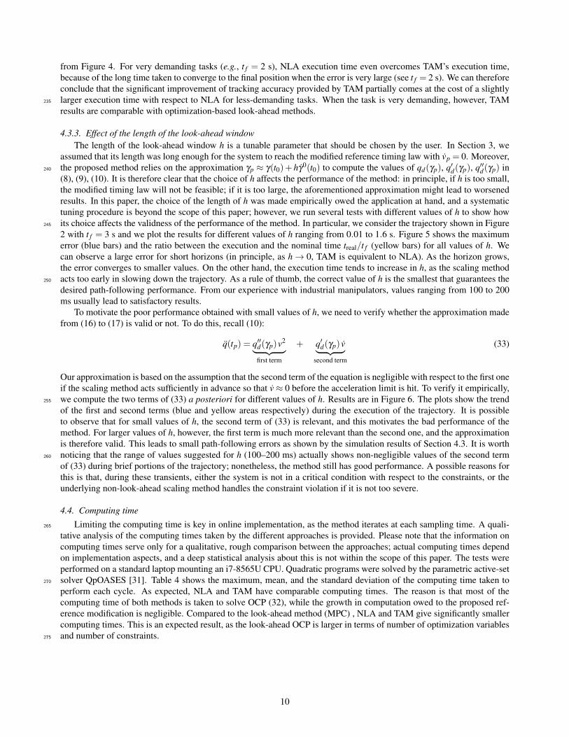
4.3.3. Effect of the length of the look-ahead windowThe length of the look-ahead window h is a tunable parameter that should be chosen by the user. In Section 3, we

assumed that its length was long enough for the system to reach the modified reference timing law with vp = 0. Moreover,the proposed method relies on the approximation γp ≈ γ(t0)+hγ0(t0) to compute the values of qd(γp), q′d(γp), q′′d(γp) in240

(8), (9), (10). It is therefore clear that the choice of h affects the performance of the method: in principle, if h is too small,the modified timing law will not be feasible; if it is too large, the aforementioned approximation might lead to worsenedresults. In this paper, the choice of the length of h was made empirically owed the application at hand, and a systematictuning procedure is beyond the scope of this paper; however, we run several tests with different values of h to show howits choice affects the validness of the performance of the method. In particular, we consider the trajectory shown in Figure245

2 with t f = 3 s and we plot the results for different values of h ranging from 0.01 to 1.6 s. Figure 5 shows the maximumerror (blue bars) and the ratio between the execution and the nominal time treal/t f (yellow bars) for all values of h. Wecan observe a large error for short horizons (in principle, as h→ 0, TAM is equivalent to NLA). As the horizon grows,the error converges to smaller values. On the other hand, the execution time tends to increase in h, as the scaling methodacts too early in slowing down the trajectory. As a rule of thumb, the correct value of h is the smallest that guarantees the250

desired path-following performance. From our experience with industrial manipulators, values ranging from 100 to 200ms usually lead to satisfactory results.

To motivate the poor performance obtained with small values of h, we need to verify whether the approximation madefrom (16) to (17) is valid or not. To do this, recall (10):

q(tp) = q′′d(γp)v2︸ ︷︷ ︸first term

+ q′d(γp) v︸ ︷︷ ︸second term

(33)

Our approximation is based on the assumption that the second term of the equation is negligible with respect to the first oneif the scaling method acts sufficiently in advance so that v≈ 0 before the acceleration limit is hit. To verify it empirically,we compute the two terms of (33) a posteriori for different values of h. Results are in Figure 6. The plots show the trend255

of the first and second terms (blue and yellow areas respectively) during the execution of the trajectory. It is possibleto observe that for small values of h, the second term of (33) is relevant, and this motivates the bad performance of themethod. For larger values of h, however, the first term is much more relevant than the second one, and the approximationis therefore valid. This leads to small path-following errors as shown by the simulation results of Section 4.3. It is worthnoticing that the range of values suggested for h (100–200 ms) actually shows non-negligible values of the second term260

of (33) during brief portions of the trajectory; nonetheless, the method still has good performance. A possible reasons forthis is that, during these transients, either the system is not in a critical condition with respect to the constraints, or theunderlying non-look-ahead scaling method handles the constraint violation if it is not too severe.

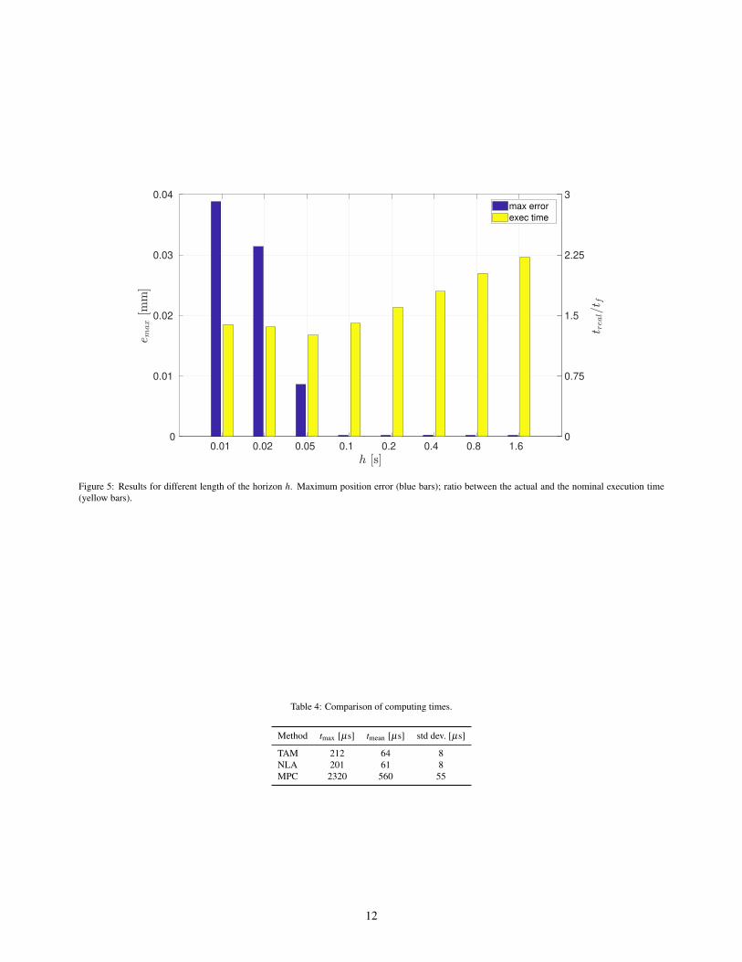
4.4. Computing time

Limiting the computing time is key in online implementation, as the method iterates at each sampling time. A quali-265

tative analysis of the computing times taken by the different approaches is provided. Please note that the information oncomputing times serve only for a qualitative, rough comparison between the approaches; actual computing times dependon implementation aspects, and a deep statistical analysis about this is not within the scope of this paper. The tests wereperformed on a standard laptop mounting an i7-8565U CPU. Quadratic programs were solved by the parametric active-setsolver QpOASES [31]. Table 4 shows the maximum, mean, and the standard deviation of the computing time taken to270

perform each cycle. As expected, NLA and TAM have comparable computing times. The reason is that most of thecomputing time of both methods is taken to solve OCP (32), while the growth in computation owed to the proposed ref-erence modification is negligible. Compared to the look-ahead method (MPC) , NLA and TAM give significantly smallercomputing times. This is an expected result, as the look-ahead OCP is larger in terms of number of optimization variablesand number of constraints.275

10

-0.1 0 0.1 0.2 0.3 0.4 0.5

0.3

0.35

0.4

0.45

0.5

0.55

0.6

0.65

0.7

nominal

NLA

MPC

TAM0.08 0.09 0.1 0.11 0.12

0.4

0.41

0.42

0.43

0.44

0.45

0.46

0.32 0.325 0.33 0.335 0.34

0.46

0.465

0.47

0.475

0.48

0.485

(a) t f = 5 s

-0.1 0 0.1 0.2 0.3 0.4 0.5

0.3

0.4

0.5

0.6

0.7

nominal

NLA

MPC

TAM

0.32 0.325 0.33 0.335

0.47

0.475

0.48

0.485

0.49

(b) t f = 4 s

-0.1 0 0.1 0.2 0.3 0.4 0.5

0.3

0.35

0.4

0.45

0.5

0.55

0.6

0.65

0.7

nominal

NLA

MPC

TAM

(c) t f = 3 s

-0.1 0 0.1 0.2 0.3 0.4 0.5

0.3

0.35

0.4

0.45

0.5

0.55

0.6

0.65

0.7

nominal

NLA

MPC

TAM

(d) t f = 2 s

Figure 4: Simulation results. Path performed by the different methods: nominal path (black dots); TAM (solid black lines); NLA (dotted red lines);MPC (dashed green lines).

Table 1: Translation error for different nominal trajectory times t f .

t f emax [m] emean [m][s] TAM NLA MPC TAM NLA MPC

5.0 1.33 ·10−4 5.30 ·10−3 1.55 ·10−4 2.55 ·10−5 2.98 ·10−4 2.67 ·10−5

4.0 1.71 ·10−4 1.78 ·10−2 1.98 ·10−4 3.58 ·10−5 1.95 ·10−3 3.93 ·10−5

3.0 2.29 ·10−4 4.65 ·10−2 2.01 ·10−4 5.04 ·10−5 7.44 ·10−3 4.99 ·10−5

2.0 3.85 ·10−4 1.43 ·10−1 2.99 ·10−4 8.43 ·10−5 4.05 ·10−2 1.03 ·10−4

Table 2: Orientation error for different nominal trajectory times t f .

t f emax [rad] emean [rad][s] TAM NLA MPC TAM NLA MPC

5.0 6.44 ·10−5 7.62 ·10−3 8.06 ·10−5 6.79 ·10−7 4.35 ·10−4 1.02 ·10−6

4.0 7.82 ·10−5 2.51 ·10−2 8.98 ·10−5 1.04 ·10−6 3.05 ·10−3 1.33 ·10−6

3.0 8.35 ·10−5 6.37 ·10−2 9.77 ·10−5 1.85 ·10−6 1.11 ·10−2 1.55 ·10−6

2.0 8.63 ·10−5 4.19 ·10−1 9.91 ·10−5 3.11 ·10−6 1.11 ·10−1 2.01 ·10−6

Table 3: Trajectory execution time for different nominal trajectory times t f .

t f treal [s] treal/t f tTAMreal −tNLA

realt f

·100[s] TAM NLA MPC TAM NLA MPC

5.0 5.79 5.42 5.25 1.15 1.08 1.05 +7.44.0 5.22 4.81 4.54 1.30 1.20 1.14 +10.23.0 4.88 4.36 3.94 1.63 1.45 1.31 +17.32.0 4.71 5.15 3.85 2.35 2.58 1.93 −22.0

11

0.01 0.02 0.05 0.1 0.2 0.4 0.8 1.6 0

0.01

0.02

0.03

0.04

0

0.75

1.5

2.25

3

max error

exec time

Figure 5: Results for different length of the horizon h. Maximum position error (blue bars); ratio between the actual and the nominal execution time(yellow bars).

Table 4: Comparison of computing times.

Method tmax [µs] tmean [µs] std dev. [µs]

TAM 212 64 8NLA 201 61 8MPC 2320 560 55

12

0 1 2 3 4 5

0

10

20

30

40

50

60

70

first term + second term

first term

(a) h = 0.02 s

0 1 2 3 4 5

0

5

10

15

20

25

30

first term + second term

first term

(b) h = 0.05 s

0 1 2 3 4 5

0

5

10

15

20

first term + second term

first term

(c) h = 0.1 s

0 1 2 3 4 5 6

0

5

10

15

20

first term + second term

first term

(d) h = 0.2 s

0 1 2 3 4 5 6

0

5

10

15

20

first term + second term

first term

(e) h = 0.4 s

0 1 2 3 4 5 6 7

0

5

10

15

20

first term + second term

first term

(f) h = 0.8 s

Figure 6: Evaluation of the approximation on (33); results for different length of the horizon h. First term of (33) (yellow area); sum of first and secondterms of (33) (blue area). Results for h = 0.01 and 1.6 s are not shown for the sake of brevity.

13

5. Experimental results

In this section, we assess the algorithms’ performance on a real robot with a (non-ideal) controller to verify whetherthe improvements given by the proposed method are still significant, despite the tracking error introduced by the motioncontroller. The experiments are shown also in the video accompanying this paper.

5.1. Setup280

Experimental tests were performed on a 6-degree-of-freedom manipulator. The setup consists of a Universal RobotsUR10, version 3.5, controlled by means of a ROS-based control architecture. The controller consists of a cascade scheme:a position control loop runs in ROS Kinetic on Ubuntu 16.04 and communicates with the robot velocity controller via aTCP connection with sampling rate equal to 125 Hz. The proposed method could actually run at higher sampling rates(according to the computing times shown in Section 4.4), but 125 Hz is the maximum sampling rate accepted by TCP285

interface of the robot at hand, which therefore acts as a bottleneck for the whole system. The outer loop is a proportionalcontroller with sampling rate equal to 125 Hz and gain equal to 7, plus a velocity feedforward term. The inner velocityloop is the built-in control system. The outputs of the tested methods are given as reference to the low-level controllerwith sampling period T = 8 ms (i.e., the sampling period of the outer loop). The measured robot configuration is acquiredfrom the robot encoders with sampling rate equal to 125 Hz, and the velocity and acceleration are obtained a posteriori290

via numerical differentiation. Torques are estimated by multiplying the motor currents by the torque constant of eachmotor. Currents are measured through the robot built-in current sensor and communicated at 125 Hz through the TCPinterface of the robot; the values of the torque constants of each motor can be found in [28]. As already mentioned, thedynamics parameters needed in the torque limits (23) are publicly available on the website of the robot manufacturer andare discussed in details in [28]. Velocity, acceleration, and torque limits have been set to (29).295

5.2. Compared methods, tests, and settingsThe proposed method (TAM), the non-look-ahead method (NLA), and the optimization-based look-ahead method

(MPC) are compared as described in Section 4.2. Maximum and mean path-following errors (emax and emean) and theexecution time (treal) are evaluated. Path-following errors are computed for both the planned and measured trajectories.The former refers to the trajectory computed by the scaling algorithms and then given as reference to the robot controller.300

The latter are computed from the actual joint coordinates measured by the joints’ encoders. Cartesian positions andorientations are then computed by applying forward kinematics to the joint coordinates at each time instant. Definitionsof emax, emean, and treal are given in Section 4.2.

The robot task is a sine curve in the xz-plain defined as:

Γxyz =(

π/3+0.6−0.5γ, 0.8, 0.4+0.2 sin(4πγ))

m, (34)

where γ ∈ [0, 1]. During the task, the end-effector orientation should be orthogonal to the yz-plain. The nominal timinglaw γ0 is a seven-trait-acceleration function as shown in Figure 3. Different values of t f are tested (note that the trajectory305

becomes more and more demanding as t f decreases).

5.3. ResultsResults are shown in Tables 5 and 6. The case t f = 5 s provides a nominal trajectory that is always within the

robot limits. It is therefore taken as reference case to evaluate the performance of the following trajectories. For theless demanding case (t f = 3.5 s), all methods give similar results and are successful in slowing down the trajectory to310

preserve the geometrical path (errors are comparable to the non-saturated case t f = 5 s). As the nominal trajectories getmore demanding, NLA’s errors grow significantly, while TAM and MPC are still able to follow the path accurately. Forexample, for t f = 1.5 s, TAM’s path-following error is in the order of 0.1 mm, while NLA drifts from the nominal pathof about 5 cm. This can be noticed in Figure 7a, which shows the path performed by the three planners: TAM and MPCfollow the curve accurately; NLA gives large overshoots during narrow curves, according to the behaviors analyzed in315

Section 4.3. It is worth stressing that the improvement due to the proposed method is evident also from the measureddata (Tables 5b and 6b). In other words, TAM’s improvement is relevant not only under ideal conditions (i.e., with idealmotion control as in Section 4), but also when the motion tracking error is taken into account.

Regarding the execution times, simulation results are confirmed again. Results are shown in Table 7. MPC givesoverall better results. TAM and NLA have comparable execution times in less demanding tasks, while TAM outperforms320

NLA as the task becomes more demanding (up to -60% for t f = 1.5 s). This is clear also from Figure 7b, which showsthe resulting timing laws for t f = 1.5 s: MPC and TAM’s timing law resembles the nominal one (dilated in time); MPC isthe faster among the three; NLA has an irregular and slow trend.

14

Table 5: Translation error for different nominal trajectory times t f .

(a) From planned motion

t f emax [m] emean [m][s] TAM NLA MPC TAM NLA MPC

5.0 5.1 ·10−5 5.7 ·10−5 4.9 ·10−5 6.1 ·10−6 6.9 ·10−6 5.9 ·10−6

3.5 7.1 ·10−5 8.9 ·10−5 6.8 ·10−5 1.3 ·10−5 2.6 ·10−5 1.2 ·10−5

3.0 7.6 ·10−5 1.0 ·10−4 9.1 ·10−5 1.5 ·10−5 4.9 ·10−5 2.2 ·10−5

2.5 9.2 ·10−4 1.5 ·10−2 1.2 ·10−4 2.3 ·10−5 7.5 ·10−4 3.4 ·10−5

2.0 1.1 ·10−4 4.1 ·10−2 1.9 ·10−4 1.1 ·10−5 3.8 ·10−3 1.3 ·10−5

1.5 1.3 ·10−4 5.5 ·10−2 2.1 ·10−4 2.4 ·10−5 5.1 ·10−3 3.1 ·10−5

(b) From measured motion

t f emax [m] emean [m][s] TAM NLA MPC TAM NLA MPC

5.0 1.6 ·10−3 1.4 ·10−3 1.5 ·10−3 2.5 ·10−4 2.8 ·10−4 2.5 ·10−4

3.5 2.6 ·10−3 2.3 ·10−3 2.3 ·10−3 4.5 ·10−4 4.5 ·10−4 4.1 ·10−4

3.0 3.3 ·10−3 2.0 ·10−2 3.0 ·10−3 6.1 ·10−4 1.8 ·10−3 5.9 ·10−4

2.5 3.7 ·10−3 6.1 ·10−2 3.6 ·10−3 6.9 ·10−4 9.3 ·10−3 8.5 ·10−4

2.0 2.4 ·10−3 6.1 ·10−2 3.1 ·10−3 4.5 ·10−4 9.6 ·10−3 4.4 ·10−4

1.5 2.3 ·10−3 7.6 ·10−2 4.0 ·10−3 5.1 ·10−4 9.6 ·10−3 7.7 ·10−4

Table 6: Orientation error for different nominal trajectory times t f .

(a) From planned motion

t f emax [rad] emean [rad][s] TAM NLA MPC TAM NLA MPC

5.0 2.6 ·10−6 2.6 ·10−6 1.9 ·10−6 1.0 ·10−6 1.0 ·10−6 7.1 ·10−7

3.5 7.0 ·10−6 8.6 ·10−6 6.7 ·10−6 2.2 ·10−6 3.6 ·10−6 1.2 ·10−6

3.0 2.4 ·10−5 4.3 ·10−3 2.1 ·10−5 3.2 ·10−6 1.4 ·10−4 1.1 ·10−6

2.5 2.5 ·10−5 3.0 ·10−2 6.0 ·10−5 3.1 ·10−6 3.7 ·10−3 8.9 ·10−6

2.0 2.2 ·10−5 1.2 ·10−1 8.3 ·10−4 3.0 ·10−6 2.2 ·10−2 1.8 ·10−4

1.5 2.4 ·10−5 1.8 ·10−1 2.3 ·10−3 3.0 ·10−6 3.4 ·10−2 3.4 ·10−4

(b) From measured motion

t f emax [rad] emean [rad][s] TAM NLA MPC TAM NLA MPC

5.0 3.6 ·10−3 3.6 ·10−3 3.5 ·10−3 7.0 ·10−4 7.1 ·10−4 6.7 ·10−4

3.5 7.7 ·10−3 7.9 ·10−3 6.8 ·10−3 1.2 ·10−3 1.3 ·10−3 1.4 ·10−3

3.0 8.3 ·10−3 1.7 ·10−2 6.4 ·10−3 1.9 ·10−3 2.6 ·10−3 2.0 ·10−3

2.5 1.3 ·10−2 3.5 ·10−2 9.9 ·10−3 2.1 ·10−3 4.5 ·10−3 2.2 ·10−3

2.0 7.2 ·10−3 6.3 ·10−2 9.9 ·10−3 1.3 ·10−3 8.3 ·10−3 3.0 ·10−3

1.5 7.0 ·10−3 8.2 ·10−2 1.2 ·10−2 1.2 ·10−3 1.1 ·10−2 1.4 ·10−3

Finally, as an example, the trends of the joint configuration, velocities, and accelerations for t f = 2 s are representedin Figure 8. Dashed gray lines are the nominal timing laws (γ0 and its velocity and acceleration). From Figure 8c, it325

is interesting to point out that the nominal timing law significantly exceeds the acceleration limits (dashed blue lines).Nonetheless, thanks to the scaling algorithms, the joint accelerations and velocities are always kept within the bounds,except for few acceleration spikes due to measurement noise and the motion controller actions. It is also worth stressingthat TAM’s trends are much smoother than NLA’s ones, with consequent minor stress of the robot actuators.

15

0 0.1 0.2 0.3 0.4 0.5 0.6

0.1

0.2

0.3

0.4

0.5

0.6

0.7

start

end

nominal

TAM

NLA

MPC

(a) Path

0 1 2 3 4 5

0

0.2

0.4

0.6

0.8

1

nominal

TAM

NLA

MPC

(b) Timing law

Figure 7: Resulting path and timing law for t f = 1.5 s.

16

Table 7: Trajectory execution time for different nominal trajectory times t f .

t f treal [s] treal/t f tTAMreal −tNLA

realt f

·100[s] TAM NLA MPC TAM NLA MPC

5.0 5.00 5.00 5.00 1.00 1.00 1.00 0.03.5 3.50 3.50 3.50 1.00 1.00 1.00 0.03.0 3.16 3.09 3.06 1.05 1.03 1.02 +2.22.5 3.04 3.20 2.84 1.22 1.28 1.14 −6.32.0 3.03 3.70 2.78 1.51 1.85 1.39 −33.71.5 2.94 3.84 2.63 1.96 2.56 1.75 −60.3

0.75

1

1.25

-1.25

-1

-0.75

0.5

1

1.5

-0.5

0

0.5

2.25

2.5

2.75

0 1 2 3 4

-1.7

-1.6

-1.5

(a) Joint positions

-2

0

2

-2

0

2

-2

0

2

-2

0

2

-2

0

2

0 1 2 3 4

-2

0

2

(b) Joint velocities

-5

0

5

-5

0

5

-10

0

10

-10

0

10

-10

0

10

0 1 2 3 4

-10

0

10

(c) Joint accelerations

Figure 8: Measured joint positions, velocities, and accelerations for t f = 2 s. Dashed gray line: nominal reference. Solid black line: TAM. Dotted redline: NLA. Dashed green line: MPC. Dashed blue line: acceleration limits.

17

6. Conclusions330

We have proposed a novel trajectory scaling method that modifies the reference timing law based on future informationabout the desired task. This can be used to confer a predictive feature on the existing trajectory scaling algorithms, butwithout falling into the computational disadvantages of model predictive control methods (i.e., higher computationalburden and the need of solving nonlinear optimization problems). Simulation and experimental results have shown thatthe proposed method significantly improves the path-following error and the total execution time of the trajectories if335

compared with non-look-ahead methods, and it shows lower computing time compared to optimization-based look-aheadmethods.

Acknowledgments

This work was partially supported by ShareWork project (H2020, European Commission – G.A. 820807) and Pick-place project (H2020, European Commission – G.A. 780488).340

References

[1] M. Elbanhawi, M. Simic, Sampling-based robot motion planning: A review, IEEE Access 2 (2014) 56–77.

[2] J. D. Gammell, S. S. Srinivasa, T. D. Barfoot, Informed RRT*: Optimal sampling-based path planning focused viadirect sampling of an admissible ellipsoidal heuristic, in: 2014 IEEE/RSJ International Conference on IntelligentRobots and Systems, 2014, pp. 2997–3004.345

[3] S. Zhang, A. M. Zanchettin, R. Villa, S. Dai, Real-time trajectory planning based on joint-decoupled optimization inhuman-robot interaction, Mechanism and Machine Theory 144 (2020) 103664.

[4] N. Zhang, W. Shang, Dynamic trajectory planning of a 3-dof under-constrained cable-driven parallel robot, Mecha-nism and Machine Theory 98 (2016) 21 – 35.

[5] C. Byner, B. Matthias, H. Ding, Dynamic speed and separation monitoring for collaborative robot applications–350

concepts and performance, Robotics and Computer-Integrated Manufacturing 58 (2019) 239–252.

[6] J. A. Marvel, R. Norcross, Implementing speed and separation monitoring in collaborative robot workcells, Roboticsand computer-integrated manufacturing 44 (2017) 144–155.

[7] D. Verscheure, B. Demeulenaere, J. Swevers, J. De Schutter, M. Diehl, Time-optimal path tracking for robots: Aconvex optimization approach, IEEE Transactions on Automatic Control 54 (2009) 2318–2327.355

[8] Q. Pham, A general, fast, and robust implementation of the time-optimal path parameterization algorithm, IEEETransactions on Robotics 30 (6) (2014) 1533–1540.

[9] A. Gallant, C. Gosselin, Extending the capabilities of robotic manipulators using trajectory optimization, Mechanismand Machine Theory 121 (2018) 502 – 514.

[10] J. Huang, P. Hu, K. Wu, M. Zeng, Optimal time-jerk trajectory planning for industrial robots, Mechanism and360

Machine Theory 121 (2018) 530 – 544.

[11] M. Boryga, A. Grabos, Planning of manipulator motion trajectory with higher-degree polynomials use, Mechanismand Machine Theory 44 (7) (2009) 1400 – 1419.

[12] U. Dincer, M. Cevik, Improved trajectory planning of an industrial parallel mechanism by a composite polynomialconsisting of bezier curves and cubic polynomials, Mechanism and Machine Theory 132 (2019) 248 – 263.365

[13] Y. Abbasi-Yadkori, J. Modayil, C. Szepesvari, Extending rapidly-exploring random trees for asymptotically optimalanytime motion planning, in: 2010 IEEE/RSJ International Conference on Intelligent Robots and Systems, 2010,pp. 127–132.

[14] ISO/TS 15066:2016 Robots and robotic devices – Collaborative robots, Standard, International Organization forStandardization, Geneva, CH (2016).370

18

[15] B. Matthias, T. Reisinger, Example application of iso/ts 15066 to a collaborative assembly scenario, in: Proceedingsof ISR 2016: 47st International Symposium on Robotics, VDE, 2016, pp. 1–5.

[16] G. Antonelli, S. Chiaverini, G. Fusco, A new on-line algorithm for inverse kinematics of robot manipulators ensuringpath tracking capability under joint limits, IEEE Trans. Rob. Autom. 19 (2003) 162–167.

[17] F. Flacco, A. De Luca, O. Khatib, Control of redundant robots under hard joint constraints: Saturation in the null375

space, IEEE Trans. Rob. 31 (2015) 637–654.

[18] C. Guarino Lo Bianco, O. Gerelli, Online trajectory scaling for manipulators subject to high-order kinematic anddynamic constraints, IEEE Trans. Rob. 27 (2011) 1144–1152.

[19] C. Guarino Lo Bianco, F. Ghilardelli, A discrete-time filter for the generation of signals with asymmetric and variablebounds on velocity, acceleration, and jerk, IEEE Transactions on Industrial Electronics 61 (2014) 4115–4125.380

[20] C. Guarino Lo Bianco, F. Ghilardelli, A scaling algorithm for the generation of jerk-limited trajectories in the oper-ational space, Robotics and Computer-Integrated Manufacturing 44 (2017) 284–295.

[21] C. Guarino Lo Bianco, F. Ghilardelli, Techniques to preserve the stability of a trajectory scaling algorithm, in:Proceedings of the IEEE International Conference on Robotics and Automation, Karlsruhe (Germany), 2013, pp.870–876.385

[22] T. Faulwasser, T. Weber, P. Zometa, R. Findeisen, Implementation of nonlinear model predictive path-followingcontrol for an industrial robot, IEEE Transactions on Control Systems Technology 25 (2017) 1505–1511.

[23] M. Faroni, M. Beschi, N. Pedrocchi, A. Visioli, Predictive inverse kinematics for redundant manipulators with taskscaling and kinematic constraints, IEEE Transactions on Robotics 35 (1) (2019) 278–285.

[24] M. Faroni, M. Beschi, C. Guarino Lo Bianco, A. Visioli, Predictive joint trajectory scaling for manipulators with390

kinodynamic constraints, Control Engineering Practice 95 (2020) 104264.

[25] A. M. Zanchettin, N. M. Ceriani, P. Rocco, H. Ding, B. Matthias, Safety in human-robot collaborative manufacturingenvironments: Metrics and control, IEEE Trans. Autom. Sci. Eng. 13 (2) (2016) 882–893.

[26] M. Lippi, A. Marino, Safety in human-multi robot collaborative scenarios: a trajectory scaling approach, in: Proc.IFAC SYROCO, Budapest (Hungary), 2018.395

[27] M. Faroni, M. Beschi, N. Pedrocchi, An MPC framework for online motion planning in human-robot collaborativetasks, in: Proceedings of the IEEE International Conference on Emerging Technologies and Factory Automation,Zaragoza (Spain), 2019.

[28] C. Gaz, E. Magrini, A. De Luca, A model-based residual approach for human-robot collaboration during manualpolishing operations, Mechatronics 55 (2018) 234 – 247.400

[29] F.-T. Cheng, T.-H. Chen, Y.-Y. Sun, Resolving manipulator redundancy under inequality constraints, IEEE Transac-tions on Robotics and Automation 10 (1994) 65–71.

[30] F. Caccavale, B. Siciliano, L. Villani, The role of Euler parameters in robot control, Asian J. of Control 1 (1999)25–34.

[31] H. Ferreau, C. Kirches, A. Potschka, H. Bock, M. Diehl, qpOASES: A parametric active-set algorithm for quadratic405

programming, Mathematical Programming Computation 6 (2014) 327–363.

19