Batch Continuous-Time Trajectory Estimation by Sean William ...
162
Batch Continuous-Time Trajectory Estimation by Sean William Anderson A thesis submitted in conformity with the requirements for the degree of Doctor of Philosophy Graduate Department of Aerospace Science and Engineering University of Toronto Copyright c 2017 by Sean William Anderson
-
Upload
khangminh22 -
Category
Documents
-
view
5 -
download
0
Transcript of Batch Continuous-Time Trajectory Estimation by Sean William ...

Batch Continuous-Time Trajectory Estimation
by
Sean William Anderson
A thesis submitted in conformity with the requirementsfor the degree of Doctor of Philosophy
Graduate Department of Aerospace Science and EngineeringUniversity of Toronto
Copyright c© 2017 by Sean William Anderson

Abstract
Batch Continuous-Time Trajectory Estimation
Sean William Anderson
Doctor of Philosophy
Graduate Department of Aerospace Science and Engineering
University of Toronto
2017
As the influence of autonomous mobile robots grows stronger on the lives of humans,
so too does the importance of robust and accurate localization (and control). Although
motion-estimation techniques utilizing passive cameras have been a core topic in robotic
research for decades, we note that this technology is unable to produce reliable results in
low-light conditions (which account for roughly half the day). For this reason, sensors that
use active illumination, such as lidar, are an attractive alternative. However, techniques
borrowed from the fields of photogrammetry and computer vision have long steered the
robotics community towards a simultaneous localization and mapping (SLAM) formulation
with a discrete-time trajectory model; this is not well suited for scanning-type sensors,
such as lidar. In this thesis, we assert that a continuous-time model of the trajectory
is a more natural and principled representation for robotic-state estimation. Practical
robotic localization problems often involve finding the smooth trajectory of a mobile
robot. Furthermore, we find that the continuous-time framework lends its abilities quite
naturally to high-rate, unsynchronized, and scanning-type sensors. To this end, we propose
novel continuous-time trajectory representations (both parametric, using weighted basis
functions, and nonparametric, using Gaussian-processes) for robotic state estimation
and demonstrate their use in a batch, continuous-time trajectory estimation framework.
We also present a novel outlier rejection scheme that uses a constant-velocity model
to account for motion distortion. The core algorithms are validated using data from a
two-axis scanning lidar mounted on a robot, collected over a 1.1 kilometer traversal.
ii

Dedication
To my mother and father – thank you for your unconditional love and support throughout
my entire academic career, for inspiring me to pursue higher levels of education, and for
pushing me to explore my talents.
iii

Acknowledgements
First and foremost, I would like to thank my supervisor, Professor Timothy D. Barfoot.
I am forever grateful for his guidance, teachings, and the time that he has invested in my
understanding of modern state estimation techniques. I would not be the researcher I am
today without Tim’s inspirational drive to conduct cutting-edge research and (seemingly)
limitless knowledge of mathematics (which he is always gracious enough to share). May
he never run out of interesting problems to sink his teeth into, and keen padawans with
whom to work.
My decision to delve in mobile robotics is largely due to the great influences I had
during my undergraduate studies. I’d like to thank Ryan Gariepy for throwing me into
the ‘wild west’ of computer vision with nothing but an OpenCV textbook, a webcam,
and a Husky Unmanned Ground Vehicle (UGV) – my career path would likely be very
different without that magical summer at Clearpath Robotics. I’d also like to thank
Steven Waslander who prepared a fantastic introductory course to mobile robotics and
inspired me to further develop my understanding of localization and navigation techniques.
Finally, a thank you to Kirk MacTavish, for countless hours of collaboration developing
our first 3D SLAM algorithm with the Microsoft Kinect, and his continued support in
graduate school with many hours of white-board and scrap-paper-based discussions.
To my colleagues and friends at the Autonomous Space Robotics Lab (ASRL), it
was a pleasure, and I hope we have the chance to work together again in the future. A
special thanks to Paul Furgale and Chi Hay Tong who paved the road for this thesis with
their pioneering work (and discussions) on continuous-time SLAM. Also, many thanks to
Colin McManus, Hang Dong, and the rest of the Autonosys operators that worked on
appearance-based lidar and collected the large gravel-pit dataset. To all the others I’ve
had the joy of working along side: Peter, Chris, Jon, Francois, Mike P., Mike W., Kai,
Pat, Tyler, Katarina, Braden, Erik, Rehman, Keith, Andrew, and Goran, thank you.
Lastly, I want to thank the National Science and Engineering Research Council
(NSERC) of Canada for their financial support through the CGS-M and CGS-D awards.
iv

Contents
1 Introduction 1
2 Appearance-Based Lidar Odometry 5
2.1 Motivation . . . . . . . . . . . . . . . . . . . . . . . . . . . . . . . . . . . 5
2.2 Lidar and the Visual-Odometry Pipeline . . . . . . . . . . . . . . . . . . 8
2.2.1 Keypoint Detection . . . . . . . . . . . . . . . . . . . . . . . . . . 10
2.2.2 Keypoint Tracking and Outlier Rejection . . . . . . . . . . . . . . 12
2.2.3 Nonlinear Numerical Solution . . . . . . . . . . . . . . . . . . . . 14
2.3 Place Recognition . . . . . . . . . . . . . . . . . . . . . . . . . . . . . . . 16
2.4 Summary . . . . . . . . . . . . . . . . . . . . . . . . . . . . . . . . . . . 16
3 Batch Estimation Theory and Applications for SLAM 18
3.1 Discrete-Time Batch SLAM . . . . . . . . . . . . . . . . . . . . . . . . . 18
3.1.1 Probabilistic Formulation . . . . . . . . . . . . . . . . . . . . . . 19
3.1.2 Gauss-Newton Algorithm . . . . . . . . . . . . . . . . . . . . . . . 22
3.1.3 Exploiting Sparsity . . . . . . . . . . . . . . . . . . . . . . . . . . 24
3.2 State Estimation Using Matrix Lie Groups . . . . . . . . . . . . . . . . . 26
3.2.1 Rotations, Transformations, and the Exponential Map . . . . . . 27
3.2.2 Homogeneous Points . . . . . . . . . . . . . . . . . . . . . . . . . 29
3.2.3 Perturbations . . . . . . . . . . . . . . . . . . . . . . . . . . . . . 30
3.3 Constant-Time Algorithms . . . . . . . . . . . . . . . . . . . . . . . . . . 32
3.3.1 Incremental SLAM . . . . . . . . . . . . . . . . . . . . . . . . . . 33
3.3.2 Relative Formulation . . . . . . . . . . . . . . . . . . . . . . . . . 34
3.4 Continuous-Time Trajectory Estimation . . . . . . . . . . . . . . . . . . 36
3.5 Summary . . . . . . . . . . . . . . . . . . . . . . . . . . . . . . . . . . . 38
v

4 Outlier Rejection for Motion-Distorted 3D Sensors 39
4.1 Related Work . . . . . . . . . . . . . . . . . . . . . . . . . . . . . . . . . 40
4.2 Problem Formulation . . . . . . . . . . . . . . . . . . . . . . . . . . . . . 41
4.3 Classic Rigid RANSAC . . . . . . . . . . . . . . . . . . . . . . . . . . . . 43
4.4 Motion-Compensated RANSAC . . . . . . . . . . . . . . . . . . . . . . . 43
4.4.1 Nonlinear Least-Squares Estimator . . . . . . . . . . . . . . . . . 44
4.4.2 Point Transformation . . . . . . . . . . . . . . . . . . . . . . . . . 45
4.5 Fast Motion-Compensated RANSAC . . . . . . . . . . . . . . . . . . . . 45
4.5.1 Euclidean Least-Squares Estimator . . . . . . . . . . . . . . . . . 46
4.5.2 Discretization of Required Transforms . . . . . . . . . . . . . . . 46
4.6 Minimal Point Set and Sufficient Conditions . . . . . . . . . . . . . . . . 46
4.7 Appearance-Based Lidar Experiment . . . . . . . . . . . . . . . . . . . . 48
4.7.1 Quality . . . . . . . . . . . . . . . . . . . . . . . . . . . . . . . . 49
4.7.2 Computational Efficiency . . . . . . . . . . . . . . . . . . . . . . . 51
4.8 Summary and Conclusions . . . . . . . . . . . . . . . . . . . . . . . . . . 52
5 Basis Function Representations for Trajectories 53
5.1 Related Work . . . . . . . . . . . . . . . . . . . . . . . . . . . . . . . . . 54
5.2 Background – Parametric Batch Estimation . . . . . . . . . . . . . . . . 55
5.3 Relative Coordinate Formulation Using Velocity . . . . . . . . . . . . . . 58
5.3.1 Velocity Profile . . . . . . . . . . . . . . . . . . . . . . . . . . . . 58
5.3.2 Kinematics . . . . . . . . . . . . . . . . . . . . . . . . . . . . . . 59
5.3.3 Perturbations to the Kinematics . . . . . . . . . . . . . . . . . . . 60
5.3.4 Parametric Batch Estimator . . . . . . . . . . . . . . . . . . . . . 63
5.3.5 Appearance-Based Lidar Experiment . . . . . . . . . . . . . . . . 71
5.4 Discussion . . . . . . . . . . . . . . . . . . . . . . . . . . . . . . . . . . . 78
5.5 Summary and Conclusions . . . . . . . . . . . . . . . . . . . . . . . . . . 80
6 Gaussian-Process Representations for Trajectories 81
6.1 Related Work . . . . . . . . . . . . . . . . . . . . . . . . . . . . . . . . . 82
6.2 Background – Gaussian Process Gauss-Newton . . . . . . . . . . . . . . . 85
6.2.1 GP Regression for Trajectory Estimation . . . . . . . . . . . . . . 85
6.2.2 GP Regression for STEAM . . . . . . . . . . . . . . . . . . . . . . 88
6.2.3 Querying the Trajectory . . . . . . . . . . . . . . . . . . . . . . . 89
vi

6.2.4 Interpolating Measurement Times . . . . . . . . . . . . . . . . . . 89
6.3 Estimating Trajectories in RN . . . . . . . . . . . . . . . . . . . . . . . . 90
6.3.1 Background – A Class of Exactly Sparse GP Priors . . . . . . . . 90
6.3.2 Nonlinear Time-Varying Stochastic Differential Equations . . . . . 94
6.3.3 Training the Hyperparameters . . . . . . . . . . . . . . . . . . . . 98
6.3.4 Mobile Robot Experiment . . . . . . . . . . . . . . . . . . . . . . 100
6.4 Estimating Trajectories in SE(3) . . . . . . . . . . . . . . . . . . . . . . 105
6.4.1 Background – Adapting for SE(3) . . . . . . . . . . . . . . . . . . 106
6.4.2 Nonlinear GP Regression for SE(3) . . . . . . . . . . . . . . . . . 108
6.4.3 A Piecewise, Locally Linear GP Prior for SE(3) . . . . . . . . . . 110
6.4.4 Stereo Camera Experiment . . . . . . . . . . . . . . . . . . . . . . 121
6.4.5 Practical Extensions . . . . . . . . . . . . . . . . . . . . . . . . . 124
6.4.6 Appearance-Based Lidar Experiment . . . . . . . . . . . . . . . . 129
6.5 Discussion . . . . . . . . . . . . . . . . . . . . . . . . . . . . . . . . . . . 133
6.6 Summary and Conclusions . . . . . . . . . . . . . . . . . . . . . . . . . . 135
7 Conclusion 137
7.1 Summary of Contributions . . . . . . . . . . . . . . . . . . . . . . . . . . 137
7.2 Future Work . . . . . . . . . . . . . . . . . . . . . . . . . . . . . . . . . . 139
A Appearance-Based Lidar Dataset 141
A.1 Gravel Pit Traversal . . . . . . . . . . . . . . . . . . . . . . . . . . . . . 142
A.2 Measurement Model . . . . . . . . . . . . . . . . . . . . . . . . . . . . . 143
A.3 Place Recognition . . . . . . . . . . . . . . . . . . . . . . . . . . . . . . . 143
Bibliography 145
vii

Notation
RM×N : The real coordinate (vector) space of M ×N matrices.a : Symbols in this font are real scalars, a ∈ R1.a : Symbols in this font are real column vectors, a ∈ RN .A : Symbols in this font are real matrices, A ∈ RM×N .1 : The identity matrix, 1 ∈ RN×N .0 : The zero matrix, 0 ∈ RM×N .
F−→a : A reference frame in three dimensions.
pc,ba : A vector from point b to point c (denoted by the super-script) and expressed in F−→a (denoted by the subscript).
pc,ba : The vector pc,ba expressed in homogeneous coordinates.SO(3) : The special orthogonal group.so(3) : The Lie algebra associated with SO(3).
Cb,a : The 3 × 3 rotation matrix that transforms vectors fromF−→a to F−→b: vc,bb = Cb,avc,ba , Cb,a ∈ SO(3).
SE(3) : The special Euclidean group.se(3) : The Lie algebra associated with SE(3).
Tb,a : The 4× 4 transformation matrix that transforms homoge-neous points from F−→a to F−→b: p
c,bb = Tb,ap
c,aa , Tb,a ∈ SE(3).
(·)∧ : The overloaded operator that transforms a vector, φ ∈ R3,into a 3 × 3 (skew-symmetric) member of so(3), and avector, ξ ∈ R6, into a 4× 4 member of se(3).
(·)∨ : The inverse operator of (·)∧.E[·] : The expectation operator.p(x) : The a priori probability density of x.
p(x|y) : The posterior probability density of x, given evidence y.N (µ,Σ) : A Gaussian probability density with mean vector µ and
covariance matrix Σ.GP(µ(t),Σ(t, t′)) : A Gaussian process with mean function µ(t) and covari-
ance function Σ(t, t′).
(·) : An a priori quantity: e.g. p(x) = N (x, P).
(·) : A posterior quantity: e.g. p(x|y) = N (x, P).(·) : An estimated quantity that acts as an operating point, or
best guess, during nonlinear state estimation.
viii

Chapter 1
Introduction
(a) An advertisement for the Central Power
and Light Company in 1957. The tag line
suggested that travel would one day be made
more enjoyable and safe through the use of
electricity. (Credit: The Victoria Advocate)
(b) A depiction of Google’s autonomous ve-
hicle prototype in 2015. The driverless ve-
hicle uses a combination of lasers, radars,
and cameras to safely navigate roads shared
with other civilian drivers. (Credit: Google)
Figure 1.1: Self-driving cars.
The dream of having autonomous mobile robots
safely traverse complex civilian settings is becoming
a reality. At the present time, computing power,
sensing capability, and the algorithms to take advan-
tage of them, have peaked at a point where industry
has begun to adopt many of the techniques devel-
oped by the academic robotics community. The
most anticipated result of this ‘collaboration’ is the
arrival of self-driving cars (see Figure 1.1), which
are predicted to be only a few years away from com-
mercialization. Several companies have been very
public about their development (and testing) of au-
tonomous vehicle technology; most notably, Google
Inc. (2015) reports having 48 autonomous vehicles
actively self-driving the public roads of Mountain
View, California, and Austin, Texas, with a collec-
tive 2 million autonomously driven kilometres since
2009. In order to enable this kind of autonomous
navigation in a safe manner, these vehicles must be
able to operate in challenging dynamic situations,
all weather and lighting conditions, and a variety
of environments (e.g., open plains, tunnels, urban
canyons, etc.).
1

Chapter 1. Introduction 2
The focus (and contributions) of this thesis are in the area of mobile robotic localization.
Plainly, a robot localization algorithm is responsible for answering the question: “Where
am I?”. Depending on the intended application, the answer can either be topological (e.g.,
city→ street→ lane), or metric (e.g., translational and rotational coordinates with respect
to a frame of reference). In modern day life, whether driving or walking to a destination,
many citizens have become accustomed to using the Global Positioning System (GPS)
on their cellular devices for real-time localization with respect to a map. Similarly, in
order to navigate an autonomous robot to a destination, we must first determine the
robot’s location in the space that our desired path is defined. However, we note that GPS
technology (although only available on Earth) is often insufficient for terrestrial robot
operation; the reliability and availability of a GPS signal is affected by many typical
operating environments (e.g., urban canyon, underground/mines, indoors/tunnels, or even
forested areas). Furthermore, the installation of infrastructure-based solutions to cover
all of the desired areas of robot operation is often prohibitively expensive, and thus we
rely on onboard sensing to satisfy our localization needs.
Arguably, the most popular onboard sensing modality for three-dimensional motion
estimation is passive camera technology, which has been a core topic in robotics research
for decades (Moravec, 1980). In particular, the use of a stereo camera to perform sparse-
feature-based visual odometry (VO) (Matthies and Shafer, 1987) has remained a leading
paradigm that enables accurate pose estimation over long distances (Sibley et al., 2010);
both the Mars Exploration Rovers (MERs) (Maimone et al., 2007) and the Mars Science
Laboratory (MSL) (Johnson et al., 2008) have used stereo-camera VO for extraterrestrial
motion estimation. Notably, without an a priori map of visual landmarks, exploratory
traverses are forced to localize with respect to a map that is built during the traversal. In
robotics this paradigm is best known as simultaneous localization and mapping (SLAM)
and is mathematically posed as a state estimation problem; that is, given some observations
of the environment, we wish to determine the state of the map, which is typically a set
of positions associated with the landmarks, and the full state of the robot, which is a
temporal set of positions, orientations, velocities, and other quantities (e.g., sensor biases
or calibration parameters), that fully describe the robot and its sensors throughout the
traversal. In contrast to exploratory traverses, we note that autonomous retrotraverse can
be enabled with separate mapping and localization phases (Furgale and Barfoot, 2010).
However, in many cases the most effective way to perform mapping is with SLAM, and
furthermore, because environments are susceptible to change, the map is kept up to date

Chapter 1. Introduction 3
(a) A photograph of the ROC6 traversing typical terrain at the Ethier Sand and Gravel pit. Note the large
shadows cast by the robot, and rocks, as the sun begins to set.
(b) A lidar-based reconstruction of the terrain, coloured by elevation. This result uses the appearance-based
lidar pipeline described in Chapter 2, and novel algorithms described in Chapters 4 and 6.
Figure 1.2: This figure shows a photograph and rendering of the ROC6 mobile robot at the
Ethier Sand and Gravel pit in Sudbury, Ontario, Canada. The large black instrument mounted
on the front of the robot is an Autonosys scanning lidar that we use for scanning-while-moving
motion estimation.
by performing SLAM during localization as well.
The downfall of vision-based SLAM, using passive camera technology, is that it relies
on consistent ambient lighting in order to find temporally similar appearance-based
features. In a real-world scenario, such as the test environment shown in Figure 1.2(a),
appearance can differ drastically with changes in lighting conditions; for example, change
in the orientation of shadows, or more severely, the total absence of light. Although
passive cameras have limited use in these severe conditions, the estimation machinery
developed to use sparse appearance-based features is principled and time-tested. Therefore,
a technology we are interested in investigating is the application of these mature visual
techniques to lidar (light radar) data, which is more robust to varying lighting conditions.
This method was originally investigated by McManus et al. (2011), and a detailed review

Chapter 1. Introduction 4
of the methodology we follow is described in Chapter 2. In short, due to the scanning
nature of the sensor, assumptions made in the traditional VO pipeline become invalid;
in particular, the methods used for both outlier rejection and the nonlinear numerical
solution require re-evaluation. We overcome these issues by developing new technologies
that consider the temporal nature of the data (see Figure 1.2(b)).
In Chapter 3 we review the mathematical principles underlying the probabilistically
based SLAM estimation problem; this review leads up to, and includes, the recent intro-
duction of a batch continuous-time trajectory estimation framework (Furgale et al., 2012).
In Chapter 4 we introduce a novel Random Sample Consensus (RANSAC) algorithm,
using a constant-velocity model, to perform outlier rejection on our motion-distorted
3D lidar data (Anderson and Barfoot, 2013a; Anderson et al., 2015b). By modelling
the robot trajectory in continuous time, we are able to account for the temporal nature
of scanning-type sensors and expose a subtle generalization of the SLAM problem that
we refer to as simultaneous trajectory estimation and mapping (STEAM). The core
contributions of this thesis adopt the STEAM approach and propose new representations
for the six-degree-of-freedom robot trajectory. Specifically, in Chapter 5 we present a
novel, parametric STEAM algorithm that is able to process loop closures in constant time
(Anderson and Barfoot, 2013b; Anderson et al., 2015b); in essence, this work moves the
relative SLAM formulation (Sibley et al., 2009) into the continuous-time framework by
estimating the body-centric velocity profile of the robot (and the spatial pose changes
associated with loop closures). In Chapter 6 we explore an alternative STEAM formula-
tion based on Gaussian-process (GP) regression; we build upon the initial work of Tong
et al. (2013) and the exactly sparse approach of Barfoot et al. (2014) by introducing:
(i) the use of nonlinear time-varying (NTV) stochastic differential equations (SDE) to
generate exactly sparse GP priors for trajectories in a vectorspace (Anderson et al., 2015a),
and (ii) a novel, exactly sparse, singularity-free, and physically motivated GP prior for
bodies translating and rotating in three-dimensional space (Anderson and Barfoot, 2015).
The core contributions from Chapters 4, 5, and 6 are all validated using a 1.1 kilometre
lidar dataset collected in Sudbury, Ontario, Canada (details in Appendix A). Finally, a
summary of the contributions and discussion of future work are presented in Chapter 7.
Chapter 2
Appearance-Based Lidar Odometry
In this chapter, we review the techniques used in a typical visual odometry (VO) pipeline
and the theory behind using lidar intensity images in lieu of passive camera imagery.
Augmentation of the VO pipeline, for lidar intensity data, was originally investigated by
McManus et al. (2011, 2012), and later followed up by Dong and Barfoot (2012) and Tong
et al. (2014). The methodologies investigated in this thesis build upon these works and are
motivated by the problems described in this chapter. In short, the standard VO pipeline is
not equipped to deal with scanning-type sensors (such as lidar or a rolling-shutter camera)
and requires new technologies to perform outlier rejection and generate a reasonable
nonlinear numerical trajectory estimate.
2.1 Motivation
In cases where an a priori map of the environment does not exist, or localization to
the map has been lost, it is necessary to perform incremental robot localization using
sequential pose change estimates (i.e., odometry) from the available sensor data. In the
most basic sense, odometry can be provided by something as simple as wheel encoders;
however, wheel odometry is fairly undependable in real-world environments. For example,
Matthies et al. (2007) note that (owing to sand) the MERs had a slip rate of 95% on
a 20 degree incline. Although we would typically expect better wheel odometry from a
modern automobile on an asphalt road, more reliable sensing is a necessity.
Vision-based methods have proven to provide reliable and accurate odometric estimates
(in both position and orientation) over long distances (Konolige et al., 2007; Sibley et al.,
2010). These methods operate by identifying and tracking a sparse set of recognizable,
5

Chapter 2. Appearance-Based Lidar Odometry 6
static features across a sequence of images. Camera geometry can then be used to solve
for both the 3D positions of the static features (i.e., landmarks) and the temporal poses1
of the camera. This style of optimization problem is described as bundle adjustment (BA)
and can trace its heritage to the stitching of aerial photography (Brown, 1958). Owing to
the restrictions of computing power, early applications of BA to mobile robotics focused
on a simplified version of the problem, in which stereo-triangulated points were aligned
in a Euclidean frame (Moravec, 1980); this work was later refined (Matthies and Shafer,
1987; Matthies, 1989) and eventually deployed on the MERs (Maimone et al., 2006, 2007)
to provide accurate and reliable odometry estimates on Mars.
As described previously, the problem with using passive cameras as the primary
sensing modality for a robotic platform is that the provided appearance information
is highly dependent on external lighting conditions. The most obvious failure mode of
VO is during low-light conditions (or even complete darkness), when tracking features
reliably becomes difficult (or impossible). Even during ‘daylight’ conditions, Matthies
et al. (2007) specifically note a VO failure on the MERs when the dominant features
were tracking the rover’s own shadow. In an attempt to enable dark navigation with
a passive stereo camera rig, Husmann and Pedersen (2008) used an LED spotlight to
show the promise of High Dynamic Range (HDR) imaging in lunar-analogue conditions;
using this method, it was noted that view range is a limiting factor due to inverse-square
illumination drop off, and that very specialized camera hardware would be required to
enable HDR imaging during continuous locomotion. While vision-based techniques have
been widely adopted due to the low cost and availability of passive camera technology,
we note that photogrammetry techniques are not restricted to the human-visible light
spectrum (this foreshadows the lidar-based technique we review in Section 2.2). An
interesting use of the infrared spectrum was presented by Rankin et al. (2007) in their
work on negative obstacle detection using a thermal camera.
Active sensors, such as lidar, enable more robust odometry under varying lighting
conditions. Furthermore, the wealth of geometric information provided by lidar range mea-
surements have made the sensors very popular for mapping both 2D and 3D environments.
In order to align scans taken from different locations, a wide range of laser-based odometry
techniques have been developed. For 3D pose estimation, a 3D lidar ‘scan’ is traditionally
constructed by concatenating swathes of temporal lidar data into a single point cloud.
1In this thesis, pose is used to indicate both a position and orientation.

Chapter 2. Appearance-Based Lidar Odometry 7
The basis of many point cloud alignment techniques is the Iterative Closest Point (ICP)
algorithm (Besl and McKay, 1992), which iteratively minimizes the least-squared Eu-
clidean error between nearest-neighbour points. Although the basic ICP algorithm is
fairly naive, it can provide impressive odometry estimates when applied sequentially
(Nuchter et al., 2007). There exist a multitude of works based on ICP that typically
modify the optimization problem by using additional information extracted from the point
cloud, such as surface normals or curvatures; Pomerleau et al. (2015) provide an excellent
survey. In general, registration techniques that work with the full dense point clouds tend
to be computationally intensive, and struggle to run online2. An alternative strand of
registration techniques focus on compressing a point cloud into a much smaller number
of points (or features) with a set of associated statistics that retain information about
the original structure. The most successful ‘compression’ techniques in this area of point
cloud registration are the Normalized Distributions Transform (NDT) (Magnusson et al.,
2007) and surfel (surface element) (Zlot and Bosse, 2012) representations; notably, both
techniques use a form of discretization on the points (such as voxelization), followed by an
eigen decomposition of the second-order statistics within each voxel. Pathak et al. (2010)
also achieve online performance with lidar by using a method in which large segments of
lidar data are ‘compressed’ into planar features for fast, closed-form pose-graph-relaxation;
notably their technique relies on stop-and-go motion to avoid motion-distortion over the
large planar features.
Though the use of geometric information has provided impressive odometric results,
it is interesting to note that the secondary lidar data product (i.e., intensity/reflectance
information) is largely discarded by most of the robotic literature. Most applications of
geometric-based lidar odometry have been in urban areas, or mines, where walls, ridges,
and other rich geometric information is typically present; in contrast, a road through
an open plain represents a failure mode for most of these algorithms – using intensity
information, such as the return from white, dashed lane markings, could prevent this
failure. Early work by Neira et al. (1999) investigated the use of intensity and range
images for localization against a known map. Prominent work by Levinson (2011) has
showed the use of lidar intensity information to enable localization and dark navigation
of an autonomous vehicle.
2In robotics, online performance typically implies that the result of an algorithm can be computedbefore the next measurement to be processed arrives.

Chapter 2. Appearance-Based Lidar Odometry 8
(a) The ROC6 mobile rover, equipped with an Au-
tonosys LVC0702 lidar and a Thales DG-16 Differ-
ential GPS unit.
NoddingMirror
Polygonal Mirror(8000 RPM)
Laser Rangender
Vertical Scan Dir.
Landmark
r1,2
r0,1
r
F→p
F→k
F→l
(b) Schematic of the Autonosys LVC0702 (Dong
et al., 2013), showing the nodding and hexagonal
mirrors used to achieve an image-style scan pattern.
Figure 2.1: The Autonosys LVC0702 is a high-framerate amplitude modulated continuous wave
(AMCW) lidar with a pulse repetition rate (PRR) of 500,000 points per second and maximum
range of ∼50 meters. In our experiments, the Autonosys was configured to have a 90 horizontal
and 30 vertical field of view, and produce 480× 360 images at 2 Hz.
Figure 2.2: This figure depicts corresponding intensity (left) and range (right) images formed
using data from the Autonosys lidar and the methodology developed by McManus et al. (2011).
In this process, image ‘creation’ using lidar is best described as pushing swathes of temporally
sequential lidar scans into a rectilinear image format (where pixel rows and columns roughly
correspond to elevation and azimuth angles). In reality, the robot has moved up to 25 cm during
the 0.5 s it takes to acquire these ‘images’.
2.2 Lidar and the Visual-Odometry Pipeline
Most of the experiments in this thesis leverage a technique, initially explored by McManus
et al. (2011), which fuses the intensity information provided by lidar with the mature
and computationally efficient, vision-based algorithms. The keystone in merging these

Chapter 2. Appearance-Based Lidar Odometry 9
Figure 2.3: This figure shows an example intensity image captured using the Autonosys LVC0702
two-axis scanning lidar. The nonaffine image distortion is caused by a yaw-type motion during
image acquisition. Note the irregular deformation of the square checkerboard pattern.
technologies is the use of a two-axis scanning lidar sensor with high-resolution intensity
information and a fairly high acquisition rate; specifically, we investigate the use of
an Autonosys LVC0702, as seen on our robot in Figure 2.1. We then use the method
developed by McManus et al. (2011) to form the lidar intensity and range data into
images, as seen in Figure 2.2. Sparse appearance-based features are then extracted from
the intensity images and temporally matched. This tactic allows us to perform visual
odometry even in complete darkness (Barfoot et al., 2013).
As with any meshing of technologies, there are often new machineries that need to be
developed. In this case, the development of vision-based algorithms have long assumed
the use of imaging sensors with a global shutter, which are well suited to discrete-time
problem formulations. In contrast to a charge-coupled device (CCD) that has a global
shutter, the slow vertical scan of the Autonosys causes nonaffine image distortion, as
seen in Figure 2.3, based on the velocity of the robot and the capture rate of the sensor.
This is similar in nature to rolling-shutter cameras that use complementary metal-oxide-
semiconductor (CMOS) technology; these scanning-type sensors are often avoided in
robotics due to the added complexity of rolling-shutter-type distortions. In the presence
of motion-distorted imagery, there are three steps in which the traditional visual pipeline
is affected (shown in Figure 2.4): (i) feature extraction, (ii) outlier rejection, and (iii) the
nonlinear numerical solution. In order to adapt these vision-based technologies to use
scanning sensors, this thesis proposes novel methods for both outlier rejection and a
nonlinear numerical solution.

Chapter 2. Appearance-Based Lidar Odometry 10
3) Extract SURF Features
1) Create Imagestack
2) Post Process Intensity Data
4) Feature Tracking
5) Outlier Rejection
6) Place Recognition
7) Nonlinear numerical solution
Raw Lidar Data
Motion Estimate
PreviousImagestack and SURF
Figure 2.4: This figure depicts the typical data processing pipeline used for visual odometry
with lidar intensity images (McManus et al., 2013). Beginning with new data, an imagestack is
formed from the intensity, elevation, azimuth, range, and time information. The intensity image
is then post processed, SURF features are extracted, and then matched against features from
the previous image. Outlier rejection (typically a RANSAC algorithm) is then used to qualify a
likely set of inliers from the proposed feature correspondences. In parallel, a place recognition
module may be used to identify whether or not we have visited ‘this’ location previously. Finally,
a nonlinear numerical solution is used to produce a motion/localization estimate. Take special
note that this pipeline is affected by motion distortion in the three highlighted modules: feature
extraction (due to nonaffine image distortion), outlier rejection (due to assumptions made by
traditional RANSAC models), and the nonlinear numerical solution (due to the discrete nature
of the trajectory representation used by typical pose estimation methods).
2.2.1 Keypoint Detection
The experiments in this thesis closely follow the methodology laid out by McManus et al.
(2011) for lidar-based image creation and sparse-feature extraction. In our experiments,
the Autonosys was configured to produce 480× 360 resolution lidar scans at 2 Hz. These
scans are stored as imagestacks, which are a collection of 2D images, containing intensity,
elevation, azimuth, range, and timestamp data. Each pixel in an imagestack corresponds
to a single, individually timestamped, lidar measurement. Notably, the raw intensity
images are post-processed to make them suitable for feature extraction; this is done by
applying an adaptive histogram to equalize areas of high and low reflectance, followed by
a low-pass Gaussian filter.
After processing the intensity images, keypoints are extracted. The goal of keypoint
detection is to find distinctive points in an image that can be robustly tracked as long
as they stay in view. Sparse appearance-based feature extraction is a popular strand
of research in computer vision. Each feature extraction algorithm typically involves
a keypoint detection scheme and a feature descriptor scheme. After the detector has
found an interesting keypoint (typically a corner, edge, or blob), a descriptor algorithm
Chapter 2. Appearance-Based Lidar Odometry 11
Figure 2.5: Qualitative results from the 24-hour experiment conducted by McManus et al.
(2011) comparing intensity images captured from an Optec ILRIS3D survey-grade lidar (top row)
against passive camera imagery (bottom row) at three different times (13:38, 18:12, and 05:43).
Extracted SURF features are overlaid – blue indicating a light blob on a dark background and
red indicating a dark blob on a light background. Note the robustness of SURF detection (in
the top row) despite the drastic changes in lighting.
is used to compress the local image patch into a shorter sequence of values that can be
quickly compared to other keypoints for similarity. In robotics, popular feature extraction
algorithms for VO include Features from Accelerated Segment Test (FAST) (Rosten and
Drummond, 2006), Scale Invariant Feature Transforms (SIFT) (Lowe, 2004), Speeded-Up
Robust Features (SURF) (Bay et al., 2006), and more recently, several binary schemes,
such as Binary Robust Independent Elementary Features (BRIEF) (Calonder et al., 2010),
Binary Robust Invariant Scalable Keypoints (BRISK) (Leutenegger et al., 2011), and
Oriented FAST and Rotated BRIEF (ORB) (Rublee et al., 2011).
Using a survey-grade 3D lidar, McManus et al. (2011) determined that SURF extracted
from intensity imagery could be robustly matched over a 24-hour period, and were
far superior to features extracted from passive camera imagery in low-light conditions
(see Figure 2.5). SURF detects ‘blobs’ of interest at a variety of scales, and encodes

Chapter 2. Appearance-Based Lidar Odometry 12
approximations to the local gradient information used by SIFT into a 64-floating-point-
number descriptor; it has become a very popular choice since being implemented on the
Graphics Processing Unit (GPU), as it can be calculated quickly in parallel, performs well
compared to its ancestor, SIFT, and has even been used to enable quick place recognition
(Cummins and Newman, 2008). Our experiments leverage a highly parallelized SURF
implementation that runs on the GPU.
During continuous movement, intensity imagery is subject to nonaffine motion distor-
tions (due to the temporal nature of lidar technology). It is expected that the performance
of typical feature detectors and descriptors (including SURF) will degrade when the
sensor acquisition rate is inadequate for the platform speed. However, since features are
extracted locally, and the local effect of motion distortion is small, we have found that
SURF performs sufficiently well for our particular configuration (a platform speed of up
to 0.5 m/s, and an Autonosys frame rate of 2 Hz).
2.2.2 Keypoint Tracking and Outlier Rejection
Given a set of temporally acquired images and the extracted features from each image, we
must now determine the feature correspondences (i.e., matches) between the sequential
image pairs. This task is typically accomplished by proposing matches based on the
keypoint’s descriptor similarity, and then performing outlier rejection (usually based on a
geometric model) to eliminate mismatches. In robotics, the most popular way to perform
outlier rejection is RANSAC (Fischler and Bolles, 1981); although arguments can be
made for the benefits of both robust M-estimation (Huber, 1981) and joint-compatibility
methods, such as active matching (Chli and Davison, 2008). RANSAC has become
popularized as an outlier rejection scheme for VO pipelines because it is fast and suitable
for robustly estimating the parameters of a model, despite a large number of outliers.
RANSAC determines the parameters of a model by generating hypotheses and using
consensus to let the data determine the most likely one (i.e., the hypothesis with which
the majority of the data agrees). In order to generate a hypothesis, a set of data (in this
case, matches) are sampled randomly from the proposed set and used to calculate the
model; note that the number of samples that must be drawn to compute a hypothesis
is dependent on the model that is being solved. The challenge in using RANSAC is
that it is not a deterministic algorithm (unless run to exhaustion) and good performance
depends on being able to (probabilistically) draw a set of matches that all belong to

Chapter 2. Appearance-Based Lidar Odometry 13
(a) This figure shows inlying feature tracks after
using a moderate threshold on reprojection error.
Due to fast motion and a slow vertical scan, only a
small temporal band of the features are matched.
(b) This figure shows how relaxing the inlier thresh-
old (for a rigid RANSAC model) allows for a larger
number of inlying matches (green), but also intro-
duces false positives (red outliers).
Figure 2.6: Figures showing the inlying feature tracks after applying a rigid 3-point RANSAC
model on lidar data captured during fairly fast and rough motion.
the inlier set within a reasonable number of iterations. Computational improvements to
RANSAC are usually based on reducing the number of samples required to compute the
model, or determining a criterion that helps bias the random sampler toward selecting
likely inliers. The most general (monocular) model, based on epipolar geometry and the
fundamental matrix, uses 8 points (Longuet-Higgins, 1981; Hartley and Zisserman, 2000).
More suitable models for real-time performance are the monocular 5-point algorithm
(Nister, 2004), and stereo-pair, 3-point algorithm (Horn, 1987).
Direct application of the traditional 3-point RANSAC algorithm to features extracted
from motion-distorted lidar imagery results in poor outlier rejection, as seen in Figure 2.6;
the scanning nature of lidar violates the assumed rigid rotation and translation model
used by the algorithm. Early experiments conducted by McManus et al. (2013) used
the rigid model and suffered from poor correspondences. Dong and Barfoot (2011) later
employed robust M-estimation as an outlier rejection scheme and more recent work by
Tong et al. (2014) leveraged our novel RANSAC method (contributed in Chapter 4 of this
thesis). The adaptation presented in this thesis is also a 3-point RANSAC algorithm, but
uses a constant-velocity model that can account for the individual timestamps of features.
Chapter 2. Appearance-Based Lidar Odometry 14
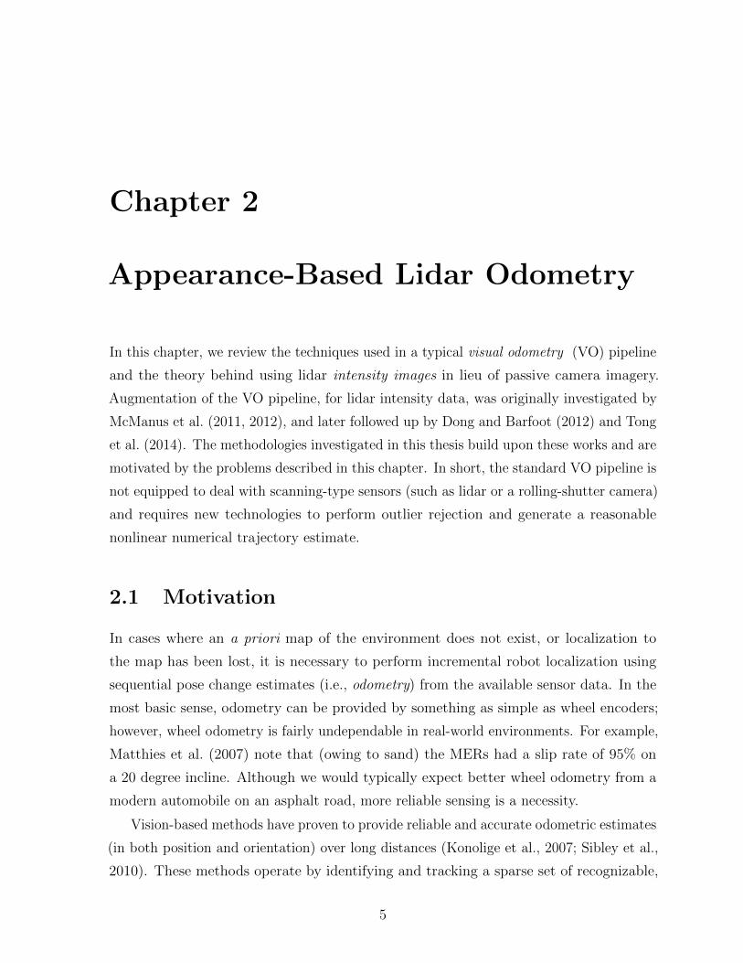
200 40 60 80 100x(m)
0
10
20
30
y(m
)Ilris VOStereo VOGPS (Fixed RTK)
Start End
(a) In this experiment, a survey grade lidar (Ilris)
was used with a stop-scan-go motion scheme to
judge the potential of lidar intensity imagery for
use in the VO pipeline (McManus et al., 2011).
Notably, the lidar-based odometry performs best∼100m from the start of the run.
200 40 60 80
0
10
y(m
)
-10
x(m)
Autonosys VOStereo VOPost Processed GPS
Start
End
(b) In this experiment, the Autonosys lidar (run-
ning at 2Hz) was used during continuous locomo-
tion to determine how drastic the effect of motion
distortion is without proper compensation (Mc-
Manus et al., 2013). Note the estimate deteriorates
quickly after a change in orientation.
Figure 2.7: These figures compare VO estimates generated by using both lidar intensity imagery
(blue) and a stereo camera (black). Ground truth was provided by GPS (red).
2.2.3 Nonlinear Numerical Solution
The final step in the VO pipeline is to estimate odometry using the feature tracks that
passed outlier rejection. A rudimentary implementation might simply re-solve the model
used by RANSAC with all of the inliers (rather than the minimal set) in a least-squares
fashion. For example, by taking advantage of depth information, the least-squares 3D-
point-alignment problem (used in the 3-point RANSAC method) can also be solved for
N -points in closed-form (Horn, 1987; Arun et al., 1987; Umeyama, 1991); owing to its
low computational cost and fairly accurate results, this method is ideal for resource
constrained systems, such as the MERs (Matthies et al., 2007).
More recently, easy access to powerful computing has begun to favour more com-
putationally intensive solutions based on batch nonlinear optimization, such as bundle
adjustment (mathematical preliminaries will be provided in Chapter 3). However, owing
to the nature of traditional VO and discrete-time SLAM formulations, they are not
well-suited to handle many challenging sensor outputs; specifically, the use of high-rate,
motion-distorted, or unsynchronized sensors all require special treatments. In our case,
scanning during continuous locomotion causes each SURF feature extracted from the
intensity imagery to be individually timestamped, and in general, traditional discrete-time
batch SLAM estimators require a pose at every measurement time. Placing a discrete
pose at each SURF measurement time causes two problems: (i) the state size becomes
computationally intractable, and (ii) with only one range/bearing measurement at each
discrete pose, the maximum likelihood (ML) problem is ill-conditioned (i.e., unobservable).
Before developing more complex machinery that allows us to properly handle these

Chapter 2. Appearance-Based Lidar Odometry 15
types of sensors, two practical experiments were conducted by McManus et al. (2011).
First, in order to justify lidar intensity imagery as a potentially suitable replacement for
passive camera imagery, an initial experiment compared lidar odometry (using a stop-
scan-go methodology to avoid motion distortion) against stereo VO (see Figure 2.7(a)).
Using the same estimation scheme, the second experiment (seen in Figure 2.7(b)) enabled
continuous locomotion to demonstrate the need for motion compensation.
Outside of research focused on solving the motion-distortion problem, there are two
commonly used strategies to improve odometry estimates from scanning sensors. The
first is to avoid the problem entirely by using a stop-scan-go motion strategy, as employed
by McManus et al. (2011), Nuchter et al. (2007), and Pathak et al. (2010) (although
this strategy has a serious impact on the platform’s freedom of motion). The second, is
to ‘pre-correct’ the distortion by using an estimate of the vehicle’s velocity – provided
by an Inertial Measurement Unit (IMU) or other external sensor. Although this type
of correction leads to satisfactory results, we note that reliance on an additional sensor
is undesirable; in particular, we note that noise from the IMU measurements, failure to
properly estimate IMU biases, and calibration error between the sensors, all become built
into the augmented scans and will contribute to irreversible odometry error. We assert
that a more general approach is to change how the robot’s trajectory is modelled in the
state, such that odometry can be estimated using motion-distorted lidar data alone; then,
additional information about the motion, such as IMU measurements, can be exploited
when, or if, it is available.
In an attempt to augment the discrete-time state formulation for scanning-type sensors,
a few works have employed the use of 3D-pose interpolation (Dong and Barfoot, 2011;
Hedborg et al., 2012; Bosse et al., 2012). The idea behind these techniques is to maintain
a small set of discrete-time keyframes that are used to interpolate a smooth 3D trajectory;
in practice, this is akin to having a discrete pose at each measurement time, where the
chosen interpolation policy enforces a strict smoothness constraint across poses that
exist between keytimes. The result is a (generally) well-conditioned problem, with a
drastically decreased state size. Notably, all three aforementioned works used time as the
interpolation variable between poses, giving rise to a reinterpretation of the formulation
as a continuous-time trajectory estimation problem. Rather than using an ad hoc linear
interpolation scheme, it is proposed that richer trajectory representations can be chosen to
better capture the true motion of the robot. Early investigations of continuous-time batch
estimation have been performed both parametrically, using a weighted sum of temporal

Chapter 2. Appearance-Based Lidar Odometry 16
basis functions (Furgale et al., 2012), and nonparametrically, using a Gaussian Process
(Tong et al., 2012). The core contributions of this thesis are based on these works; in
particular, we explore alternative trajectory representations that aim to improve both
the utility and efficiency of these methods. While more specific information about the
implementation of these methods is left to the later chapters, we note that it is the use of
these continuous-time trajectory formulations that allow us to produce accurate odometry
estimates and maps using motion-distorted lidar imagery.
2.3 Place Recognition
In this thesis, we will go beyond the VO-style nonlinear numerical solutions provided by
Dong and Barfoot (2011) and Tong et al. (2014) by taking advantage of large-scale loop
closures. In essence, by recognizing when the robot has returned to a location that it
has previously traversed, the ‘loop’ can be closed and parameters in the map (i.e., 3D
landmark positions) from the same physical location can be associated – this helps to
improve the metric accuracy of localization, as well as introduce topological linkages that
can be used for navigation. Chapters 5 and 6 each contain a novel algorithm that uses
a relative-pose formulation to process these large-scale loop closures in constant time
(background on the relative SLAM paradigm will be discussed in Chapter 3).
Taking advantage of vision algorithms once again, we note that the use of SURF allows
us to leverage existing Bag-of-Words place-recognition algorithms, such as FAB-MAP
(Cummins and Newman, 2008). However, owing to motion distortion we found that the
standard FAB-MAP methodology did not perform well – instead, we used the extension
of MacTavish and Barfoot (2014). In contrast to the original FAB-MAP algorithm, which
compares a single query image to all of the previously seen images using a Bag-of-Words
descriptor, the modification proposed by MacTavish and Barfoot (2014) describes and
compares groups of images (i.e., they use a bigger bag of words); this modification was
key in enabling more robust place recognition despite motion distortion.
2.4 Summary
In this chapter we reviewed some of the theory and literature related to using lidar
intensity imagery, rather than passive camera imagery, in the VO pipeline. The advantage
of using an active sensor, such as lidar, is that it is almost completely invariant to

Chapter 2. Appearance-Based Lidar Odometry 17
lighting conditions and allows us to operate even in complete darkness. Furthermore, by
extracting sparse appearance-based features from the intensity imagery we are able to
leverage a variety of mature techniques (e.g., feature tracking, RANSAC, Bag-of-Words
place recognition, bundle-adjustment-style estimation). The issue that arises in this fusion
of technologies is motion distortion and the fact that standard vision-based techniques
are not equipped to deal with scanning sensors. Chapters 4, 5, and 6 of this thesis will
propose novel solutions for pieces of the VO pipeline that require special care in order to
account for the temporal nature of the lidar sensor.

Chapter 3
Batch Estimation Theory and
Applications for SLAM
This chapter serves as a mathematical primer on the use of batch estimation for SLAM.
The core contributions of this thesis depend on many of the techniques described in this
chapter. The following sections will introduce: (i) probabilistic theory geared towards the
batch SLAM formulation, (ii) nonlinear optimization using the Gauss-Newton algorithm,
(iii) estimation machinery for the matrix Lie groups SO(3) and SE(3), (iv) variants of the
batch SLAM problem aimed at achieving constant-time performance, and (v) preliminaries
towards estimating a continuous-time robot trajectory.
3.1 Discrete-Time Batch SLAM
Accurately determining a robot’s position with respect to a set of obstacles, landmarks,
or path of interest (i.e., a map), is a precursor to autonomous navigation and control
of a mobile robotic system. In contrast to pure localization (against an a priori map),
simultaneous mapping is absolutely vital in traversing previously unvisited environments.
Since state-of-the-art robotic systems have set their sights on enabling long-term autonomy
in unstructured 3D environments, the importance of robust SLAM technology has only
grown. Even when an a priori map exists, online mapping remains an integral component
of long-term localization engines due to the possibility of vast scene change (e.g., weather,
lighting, or even infrastructure). Recording new ‘experiences’ for life-long SLAM has
enabled some of the most promising results (Churchill and Newman, 2013).
From a mathematical perspective, modern SLAM algorithms continue to leverage
18

Chapter 3. Batch Estimation Theory and Applications for SLAM 19
a probabilistic foundation, as it provides a principled and successful model for fusing
measurements from multiple sensors and incorporating a priori knowledge of the state.
The standard state representation for this type of problem continues to be the discrete-
time pose (and sometimes velocity) of the robot, in addition to a set of discrete landmark
positions. The origin of this formulation in the robotics community can be traced back to
the work of Smith et al. (1990), which set the stage for 2D probabilistic SLAM algorithms
to use filtering-based estimation theory (Kalman, 1960). Only much later did Lu and
Milios (1997) derive the full batch problem formulation, using odometry measurements to
smooth the trajectory between landmark observations. Notably, the discrete-time batch
SLAM problem is closely related to that of the (much earlier) bundle adjustment problem
(Brown, 1958); the unique nature of the SLAM problem is that we are estimating the
temporal pose of a single rigid body (in contrast to the individual poses of an unordered
set of aerial cameras). Exploiting the temporal nature of the measurements, a specialized
problem is formed by including an a priori motion model and measurements from other
sensors, such as wheel encoders, compass, IMU, or even lidar.
Despite the batch formulation offering a more accurate solution, filter-based algorithms,
such as the Extended Kalman Filter (EKF) (Kalman, 1960), Sigma-Point Kalman Filter
(Julier and Uhlmann, 1997), and the Particle Filter (Thrun et al., 2001), were widely used
due to their lower computational requirements and ability to run online. However, the
advancement of modern computing power has slowly favoured batch estimation techniques
that were previously too inefficient for practical use. Today, the most successful SLAM
solutions have taken advantage of the batch problem formulation (Thrun and Montemerlo,
2006; Dellaert and Kaess, 2006; Kaess et al., 2008; Sibley et al., 2009; Konolige et al.,
2010), and modern implementations have proven to provide higher accuracy solutions
(per unit of computation) over the filtering-based competitors (Strasdat et al., 2010).
3.1.1 Probabilistic Formulation
In the standard discrete-time batch SLAM formulation, there are two sets of quantities we
are interested in estimating: (i) the pose of the robot at all measurement times, x0:K , and
(ii) a set of static landmarks parameters, `0:L. In order to determine the values of x0:K
and `0:L, we typically use two sources of information. The first is a priori information,
based on our initial knowledge of the robot’s position, x0, and the (known) control inputs,

Chapter 3. Batch Estimation Theory and Applications for SLAM 20
u0:K−1, combined with a motion model:
xk+1 = f(xk,uk) + wk, (3.1)
where xk is the pose of the robot at time tk, f(·) is a nonlinear function, uk is the discretized
control input, and wk is the process noise. In order to keep this derivation relatively
straightforward we have assumed that our motion model has an additive process noise.
In general, wk could also be an input parameter of the nonlinear function f(·), as we will
later explore in Chapter 6 (for continuous-time models).
The second piece of information (used to refine the estimate), is an observation
model, which correlates our series of poses, x0:K , through measurements of common static
landmark parameters, `j,
ykj = g(xk, `j) + nkj, (3.2)
where ykj is a sensor measurement, g(·) is a nonlinear measurement model, `j is an
observed point-landmark, and nkj is the sensor noise. In this model, we have again
assumed that the noise, nkj, is additive; however, we note that for observation models
this is a much more common/fair assumption.
Taking the probabilistic approach to discrete-time batch SLAM, the maximum a
posteriori (MAP) problem we wish to solve is
x, ˆ = argmaxx,`
p(x, ` |u, y), (3.3)
where (for convenience) we have defined
x := (x0, . . . , xK) , ` := (`0, . . . , `L) , u := (x0,u0, . . . ,uK−1) , y := (y00, . . . , yKL) ,
and x, ˆ is the posterior value of x, `. An equivalent solution to (3.3) can be found
by minimizing the negative log likelihood:
x, ˆ = argminx,`
(− ln p(x, ` |u, y)) . (3.4)
By assuming that the noise variables, wk and nkj, for k = 0 . . . K, are uncorrelated, we
follow the standard Bayes’ rule derivation1 to rewrite the posterior probability density as,
ln p(x, ` |u, y) = ln p(x0 | x0) +∑k
ln p(xk+1 | xk,uk) +∑kj
ln p(ykj | xk, `j). (3.5)
1The details of the probabilistic SLAM derivation are fairly common knowledge among roboticists.However, for more details, as well as interesting discussions and demonstrations, I highly recommendboth Barfoot (2016) and Thrun et al. (2005).

Chapter 3. Batch Estimation Theory and Applications for SLAM 21
Next, we assume that the above probability densities are Gaussian by setting
x0 ∼ N (x0, P0), wk ∼ N (0,Qk), nkj ∼ N (0,Rkj), (3.6)
where x0 and P0 are the prior mean and covariance of the initial position, and the process
noise, wk, and measurement noise, nkj, are normally distributed with covariances Qk
and Rkj, respectively. Finally, by using the models in (3.1) and (3.2), and substituting
the Gaussian distributions into (3.5), and subsequently (3.4), we arrive at the typical
least-squares batch optimization problem:
x, ˆ = argminx,`
(Jp(x) + Jm(x, `) + const.
), (3.7)
where Jp(x) is a sum of Mahalanobis distances (i.e., squared-error terms) related to the a
priori data,
Jp(x) :=1
2eTp0
P−10 ep0 +
1
2
∑k
eTukQ−1k euk , (3.8)
and similarly, Jm(x, `) is a sum of Mahalanobis distances related to the observations,
Jm(x, `) :=1
2
∑kj
eTmkjR−1kj emkj , (3.9)
where the error terms are:
ep0 := x0 − x0, (3.10a)
euk := xk+1 − f(xk,uk), (3.10b)
emkj := ykj − g(xk, `j). (3.10c)
Defining the objective function,
J(x, `) := Jp(x) + Jm(x, `), (3.11)
the final MAP estimator is simply
x, ˆ = argminx,`
J(x, `) . (3.12)
By solving this nonlinear, least-squares problem, we obtain values for x and ˆ that
maximize the joint-likelihood of our data and a priori information. In the absence
of a prior (i.e., the prior is a uniform distribution over all possible robot states), this
Chapter 3. Batch Estimation Theory and Applications for SLAM 22
formulation is equivalent to the well understood maximum likelihood (ML) problem. Over
the past decade, an exploding number of works have built upon this probabilistic batch
estimation scheme to solve a variety of problems. Typical extensions include (but are
not limited to): (i) penalty, constraint, and conditioning terms that directly affect the
objective function, (ii) optimization strategies to more efficiently, or robustly, find the
optimal state, and (iii) new parameterizations for the robot or landmark states to improve
utility or performance. The remainder of this chapter will review existing tools and
extensions of the batch framework used by the contributions of this thesis.
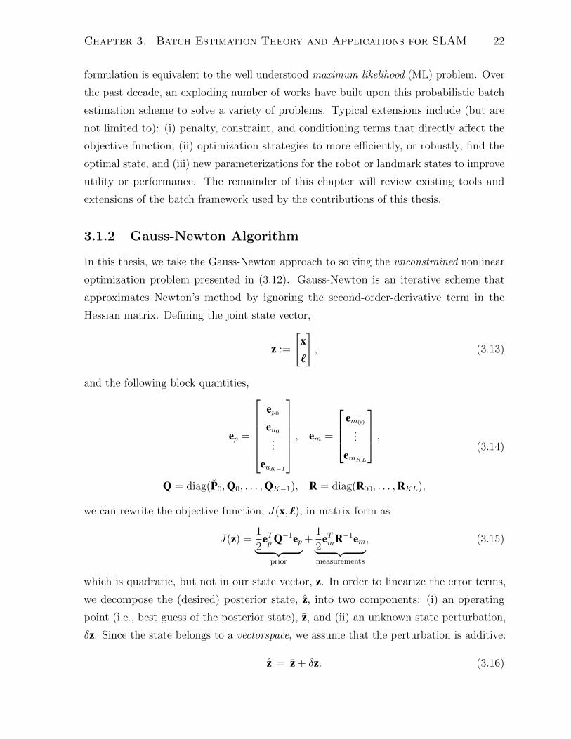
3.1.2 Gauss-Newton Algorithm
In this thesis, we take the Gauss-Newton approach to solving the unconstrained nonlinear
optimization problem presented in (3.12). Gauss-Newton is an iterative scheme that
approximates Newton’s method by ignoring the second-order-derivative term in the
Hessian matrix. Defining the joint state vector,
z :=
[x`
], (3.13)
and the following block quantities,
ep =
ep0
eu0
...
euK−1
, em =
em00
...
emKL
,Q = diag(P0,Q0, . . . ,QK−1), R = diag(R00, . . . ,RKL),
(3.14)
we can rewrite the objective function, J(x, `), in matrix form as
J(z) =1
2eTp Q−1ep︸ ︷︷ ︸
prior
+1
2eTmR−1em︸ ︷︷ ︸
measurements
, (3.15)
which is quadratic, but not in our state vector, z. In order to linearize the error terms,
we decompose the (desired) posterior state, z, into two components: (i) an operating
point (i.e., best guess of the posterior state), z, and (ii) an unknown state perturbation,
δz. Since the state belongs to a vectorspace, we assume that the perturbation is additive:
z = z + δz. (3.16)

Chapter 3. Batch Estimation Theory and Applications for SLAM 23
Therefore, by solving the intermediate problem,
δz? = argminδz
J(z + δz) , (3.17)
the optimal state perturbation, δz?, can be used to bring our best guess, z, closer to the
optimal posterior value, z. In Newton’s method, J(z) is approximated as quadratic by
using a three-term Taylor-series expansion:
J(z + δz) ≈ J(z) +
(∂J(z)
∂z
∣∣∣∣z︸ ︷︷ ︸
Jacobian
)δz +
1
2δzT(∂2J(z)
∂z∂zT
∣∣∣∣z︸ ︷︷ ︸
Hessian
)δz. (3.18)
In practice, Newton’s method is seldom used for multivariate problems since the second-
order-derivative terms in the Hessian can be difficult to compute. The Gauss-Newton
method approximates Newton’s method by simply ignoring the second-order derivatives
in the Hessian. Notably, an equivalent approximation is to simply start with a first-order
Taylor-series expansion of the error terms. Following this alternative derivation, the
nonlinear error terms in (3.10) are linearized by substituting the assumption from (3.16),
ep0(z + δz) ≈ ep0(z) + δx0, ep0(z) = x0 − x0, (3.19a)
euk(z + δz) ≈ euk(z) + δxk+1 − Fk δxk, euk(z) = xk+1 − f(xk,uk), (3.19b)
emkj(z + δz) ≈ emkj(z)−Gx,kj δxk −G`,kj δ`j, emkj(z) = ykj − g(xk, ¯j), (3.19c)
where Fk, Gx,kj, and G`,kj are the Jacobian matrices,
Fk :=∂f(xk,uk)∂xk
∣∣∣∣xk,uk
, Gx,kj :=∂g(xk, `j)∂xk
∣∣∣∣xk,¯j
, G`,kj :=∂g(xk, `j)
∂`j
∣∣∣∣xk,¯j
. (3.20)
Rearranging these quantities into matrix form, we write
ep ≈ ep − F δz, em ≈ em −G δz, (3.21)
where
ep = ep|z , em = em|z , F =∂ep∂z
∣∣∣∣z, G =
∂em∂z
∣∣∣∣z, (3.22)
and the objective function becomes,
J(z + δz) =1
2(ep − Fδz)TQ−1(ep − Fδz) +
1
2(em −Gδz)TR−1(em −Gδz). (3.23)
Taking the derivative of J(z), with respect to δz, and setting it to zero,
∂TJ(z)
∂δz= −FTQ−1(ep − Fδz)−GTR−1(em −Gδz) = 0, (3.24)

Chapter 3. Batch Estimation Theory and Applications for SLAM 24
this expression can be rearranged to find the system of linear equations
( Apri︷ ︸︸ ︷FTQ−1F +
Ameas︷ ︸︸ ︷GTR−1G︸ ︷︷ ︸
A
)δz? = FTQ−1ep + GTR−1em︸ ︷︷ ︸
b
, (3.25)
which we can solve for the optimal perturbation, δz? = A−1b. In an iterative fashion,
we then update our best guess, z← z + δz?, to convergence, and set the final posterior
estimate, z = z. Furthermore, we note that the covariance is simply
cov(δz?, δz?) = A−1. (3.26)
In order to improve the estimator’s convergence and avoid local minima, several strategies
exist to increase the robustness of this nonlinear least-squares solution. In particular,
we make use of robust M-estimation (Huber, 1981) and trust-region solvers, such as
Levenberg-Marquardt (Levenberg, 1944; Marquardt, 1963) and Powell’s Dogleg (Powell,
1970). Increasing robustness remains an active interest in the robotics community due its
importance in online systems; more recent works, such as Sunderhauf and Protzel (2012)
have focused on generalizing outlier rejection within the batch optimization framework.
To aid the following discussion on sparsity, the left- and right-hand side terms of (3.25)
have been labelled; we note that the Apri term comes from the a priori information, and
Ameas is associated with the landmark measurements.
3.1.3 Exploiting Sparsity
In general, the naive complexity of solving the system δz? = A−1b, with K measurement
times and L landmarks, is O((K + L)3). Rewriting the linear system of equations,
A δz? = b, in the 2× 2 block-form,[Axx Ax`
ATx` A``
][δx?
δ`?
]=
[bxb`
], (3.27)
we note that the left-hand side has the form,
[Axx Ax`
ATx` A``
]=
Apri︷ ︸︸ ︷[Y 00 0
]+
Ameas︷ ︸︸ ︷[U W
WT V
], (3.28)
where Y is a block-tridiagonal matrix related to the prior and Ameas is the usual arrowhead
matrix (Brown, 1958), where U and V are block-diagonal, and W is (potentially) dense.
Chapter 3. Batch Estimation Theory and Applications for SLAM 25
ep0ep0
kk k kk k
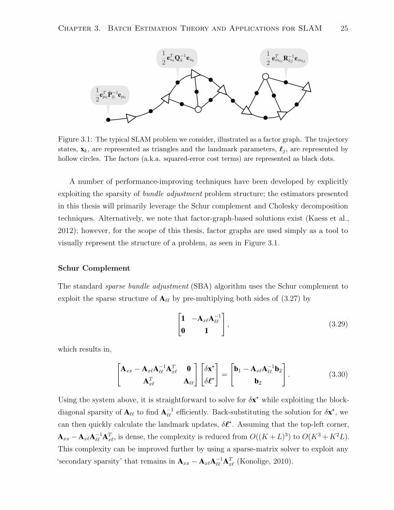
Figure 3.1: The typical SLAM problem we consider, illustrated as a factor graph. The trajectory
states, xk, are represented as triangles and the landmark parameters, `j , are represented by
hollow circles. The factors (a.k.a. squared-error cost terms) are represented as black dots.
A number of performance-improving techniques have been developed by explicitly
exploiting the sparsity of bundle adjustment problem structure; the estimators presented
in this thesis will primarily leverage the Schur complement and Cholesky decomposition
techniques. Alternatively, we note that factor-graph-based solutions exist (Kaess et al.,
2012); however, for the scope of this thesis, factor graphs are used simply as a tool to
visually represent the structure of a problem, as seen in Figure 3.1.
Schur Complement
The standard sparse bundle adjustment (SBA) algorithm uses the Schur complement to
exploit the sparse structure of A`` by pre-multiplying both sides of (3.27) by[1 −Ax`A−1
``
0 1
], (3.29)
which results in, [Axx − Ax`A−1
`` ATx` 0
ATx` A``
][δx?
δ`?
]=
[b1 − Ax`A−1
`` b2
b2
]. (3.30)
Using the system above, it is straightforward to solve for δx? while exploiting the block-
diagonal sparsity of A`` to find A−1`` efficiently. Back-substituting the solution for δx?, we
can then quickly calculate the landmark updates, δ`?. Assuming that the top-left corner,
Axx−Ax`A−1`` AT
x`, is dense, the complexity is reduced from O((K +L)3) to O(K3 +K2L).
This complexity can be improved further by using a sparse-matrix solver to exploit any
‘secondary sparsity’ that remains in Axx − Ax`A−1`` AT
x` (Konolige, 2010).

Chapter 3. Batch Estimation Theory and Applications for SLAM 26
Sparse Cholesky Decomposition
In Chapter 6, due to the problem formulation and types of experiments, a reverse situation
occurs where we potentially have many more trajectory variables than landmark variables,
L K, and so we instead wish to exploit the sparsity of Axx. This is a more complicated
situation, as Axx is block-tridiagonal, rather than block-diagonal. In this situation, sparse
(lower-upper) Cholesky decomposition offers an efficient solution,[Vxx 0V`x V``
]︸ ︷︷ ︸
V
[VTxx VT
`x
0 VT``
]︸ ︷︷ ︸
VT
=
[Axx AT
`x
A`x A``
]︸ ︷︷ ︸
A
, (3.31)
in which we are able to decompose VxxVTxx = Axx in O(K) time; this results in Vxx being
a lower-bidiagonal matrix. Sparing the details, the decomposition phase is performed in
O(L3 + L2K) time. Performing the standard forward-backward passes,
solve for d: V d = b,
solve for δz?: VT δz? = d,
where d is an intermediate variable, the system is then solved in O(L2 + LK) time.
Therefore, the total complexity is dominated by the decomposition, which is O(L3 +L2K).
Notably, this method avoids any direct matrix inversions (which can ruin sparsity and
sometimes cause numerical instability).
3.2 State Estimation Using Matrix Lie Groups
Thus far we have presented the estimation theory and mathematics for solving batch
nonlinear optimization problems with state variables that belong to a vectorspace (i.e.,
z ∈ RN). However, in robotics it is common to have state variables that describe
the orientation, or pose, of the robot in three-dimensional space. The issue with using
rotations and transformations in our probabilistic derivation is that they do not belong to a
vectorspace, but rather to the (noncommutative) matrix Lie groups: the special orthogonal
group, SO(3), and the special Euclidean group, SE(3). Specifically, without special care,
variables that exist on manifolds cannot be directly included in our unconstrained Gauss-
Newton estimator because they violate two of the tools used in our MAP derivation:
(i) the use of an unconstrained additive state perturbation, z = z + δz, δz ∈ RN , and

Chapter 3. Batch Estimation Theory and Applications for SLAM 27
(ii) the use of simple Jacobian matrices, F and G, relating the output of our motion and
observation models to changes in the state vector, z ∈ RN .
Notably, several representations exist for three-dimensional rotations; however, naively
choosing a rotation representation can yield undesirable consequences. For example,
a minimal parameterization, such as Euler angles (∈ R3), suffers from singularities,
while over-parameterized representations, such as quaternions (∈ R4), required addi-
tional constraints. In this thesis, we favour using the constraint-sensitive perturbation
schemes detailed in Barfoot and Furgale (2014)2; by using an over-parameterized (but
singularity-free) 4 × 4 homogeneous transformation matrix with a 6 × 1 (constraint-
sensitive) perturbation scheme, the typical downfalls of rotation representations (in the
Gauss-Newton context) are avoided. Note that we do not require a vectorspace state,
z ∈ RN , in order to leverage the iterative Gauss-Newton updates in (3.25), but only a
vectorspace perturbation, δz ∈ RN (assuming that the Gaussian probability densities are
properly handled). The remainder of this chapter section is used to review the mathe-
matical machinery that we leverage for unconstrained nonlinear optimizations involving
rotations, transformations, and homogeneous points.
3.2.1 Rotations, Transformations, and the Exponential Map
We begin by defining the three-dimensional reference frames, F−→a and F−→b, where a vector
from F−→a to F−→b (superscript), expressed in F−→a (subscript), is written vb,aa , and Cb,a is the
3× 3 rotation matrix that transforms vectors from F−→a to F−→b:
vb,ab = Cb,avb,aa , (3.32)
where Cb,a ∈ SO(3) and is subject to the constraints,
Cb,aCTb,a = 1, det Cb,a = 1. (3.33)
Using the exponential map, we note the closed-form expression
C(φ) := exp(φ∧) = cosφ1 + (1− cosφ)aaT + sinφa∧, (3.34)
2While this thesis provides an overview of the mathematical machinery and identities necessary toperform Gauss-Newton with transformation matrix state variables, a more detailed understanding of howthe Gaussian uncertainties are handled on SE(3) can be gained by reading Barfoot and Furgale (2014).Pertaining to optimization, Absil et al. (2009) provides an in-depth discussion of first-order, second-orderand trust-region-based techniques for problems involving matrix manifolds.

Chapter 3. Batch Estimation Theory and Applications for SLAM 28
where φ = ||φ|| is the angle of rotation, a = φ/φ is the axis of rotation, and ∧ turns
φ ∈ R3 into a 3× 3 member of the Lie algebra, so(3)(Murray et al., 1994),
φ∧ :=
φ1
φ2
φ3
∧
:=
0 −φ3 φ2
φ3 0 −φ1
−φ2 φ1 0
. (3.35)
Introducing our 4× 4 homogeneous transformation matrix definition,
Tb,a =
[Cb,a ra,bb0T 1
]≡[
Cb,a −Cb,arb,aa0T 1
], (3.36)
we note that a similar closed-form expression exists by using the exponential map,
T(ξ) := exp(ξ∧) =
[C Jρ0T 1
]∈ SE(3), (3.37)
where ξ ∈ R6, the overloaded operator, ∧, turns ξ into a 4× 4 member of the Lie algebra
se(3)(Murray et al., 1994; Barfoot and Furgale, 2014),
ξ∧ :=
[ρ
φ
]∧=
[φ∧ ρ
0T 0
], ρ,φ ∈ R3, (3.38)
the rotation matrix, C, can be computed using (3.34), or the identity
C ≡ 1 + φ∧J, (3.39)
and J is the (left) Jacobian of SO(3), with the closed-form expression
J(φ) :=
∫ 1
0
Cαdα ≡ sinφ
φ1 +
(1− sinφ
φ
)aaT +
1− cosφ
φa∧. (3.40)
To gain some intuition about J, we note that when δϕ is small
exp(δφ∧) exp(φ∧) ≈ exp((φ+ δϕ)∧), δφ = J(φ)δϕ, (3.41)
where exp(δφ∧) ∈ SO(3) is a small rotation matrix perturbing exp(φ∧) ∈ SO(3). Simi-
larly, for SE(3), when δε is small (Barfoot and Furgale, 2014, Appendix A),
exp(δξ∧) exp(ξ∧) ≈ exp((ξ + δε)∧), δξ = J (ξ)δε, (3.42)
where J (ξ) is the (left) Jacobian of SE(3),
J (ξ) :=
∫ 1
0
T αdα ≡[
J(φ) Q(ξ)
0 J(φ)
]∈ R6×6, (3.43)

Chapter 3. Batch Estimation Theory and Applications for SLAM 29
T is the adjoint transformation matrix,
T := Ad(T) = Ad
([C r0T 1
])=
[C r∧C0 C
]= exp (ξf) ∈ R6×6, (3.44)
(·)f is the SE(3) operator,
ξf =
[ρ
φ
]f:=
[φ∧ ρ∧
0 φ∧
], (3.45)
and Q(ξ) has the closed-form expression
Q(ξ) :=1
2ρ∧ + φ−sinφ
φ3 (φ∧ρ∧ + ρ∧φ∧ + φ∧ρ∧φ∧)− 1−φ2
2−cosφ
φ4
(φ∧φ∧ρ∧ + ρ∧φ∧φ∧
− 3φ∧ρ∧φ∧)− 1
2
(1−φ
2
2−cosφ
φ4 − 3φ−sinφ−φ
3
6φ5
)(φ∧ρ∧φ∧φ∧ + φ∧φ∧ρ∧φ∧) . (3.46)
Lastly, we introduce the logarithmic map,
φ = ln(C)∨ ∈ R3, ξ = ln(T)∨ ∈ R6, (3.47)
where ∨ is the inverse of the overloaded operator ∧ in (3.35) and (3.38).
3.2.2 Homogeneous Points
Using homogeneous coordinates we rewrite a point vector, pb,aa ∈ R3 as,
pb,aa := η
[pb,aa1
]=
[ε
η
]∈ R4, (3.48)
where η is a non-negative scalar that is used to improve Gauss-Newton conditioning issues
when points are infinitely far away (Triggs et al., 2000). For simplicity, the derivations
in this thesis will typically assume that η = 1. One of the key strengths in using 4× 4
homogeneous transformation matrices is how easily we can transform a homogeneous
point expressed in one frame, F−→a, to another, F−→b, in a single multiplication:
pc,bb = Tb,a pc,aa . (3.49)
We also make use of the following identities in our later derivations:
ξ∧p ≡ pξ, (3.50a)
(Tp) ≡ TpT −1, (3.50b)
where (·) is the homogeneous coordinate operator (Barfoot and Furgale, 2014),
p :=
[ε
η
]=
[η1 −ε∧
0T 0T
]∈ R4×6. (3.51)

Chapter 3. Batch Estimation Theory and Applications for SLAM 30
Figure 3.2: This figure depicts the injection of noise directly onto the SE(3) manifold for the
random variable T, where T = exp(δξ∧) T. From left to right: (i) the uncertainty of δξ ∈ R6,
(ii) a depiction of the uncertainty passed through the exponential map, (iii) the operating point,
or mean, of T, and (iv) a depiction of the random variable T on SE(3).
3.2.3 Perturbations
At this point, we have described the necessary mathematical machinery for using trans-
formations and homogeneous points to represent the state of our three-dimensional pose
estimation problem. Recalling the problem formulation set up in Section 3.1.2, we now
write our discrete set of three-dimensional robot poses as
x = T0,i,T1,i, . . . ,Tk,i, . . . ,TK,i, F−→k := F−→rob(tk), (3.52)
where F−→rob(tk) is the robot frame at the time of measurement k, and the pose state
variables, Tk,i, represent the robot pose with respect to an inertial frame, F−→i. Note that
we abuse our notation slightly, as x is not a vector; similarly, we also write z = x, `.Next, we must create the connections that allow us to use this state in the probabilistic
batch estimator we derived in Section 3.1.1. As mentioned previously, the key to taking
advantage of this formulation, despite having non-vectorspace state variables, is being
able to formulate a perturbation vector, δz ∈ RN . Similar to the vectorspace case, we
want to decompose our (desired) posterior state, z, into our best guess, z, and an unknown
perturbation, δz. For transformation matrices, this is accomplished by leveraging the
exponential map from R6 to the SE(3) manifold:
Tk,i = exp(δξ∧k,i) Tk,i, (3.53)
where Tk,i is our best guess of Tk,i, and exp(δξ∧k,i) is a small transformation matrix
that uses the perturbation vector δξk,i ∈ R6 (Barfoot and Furgale, 2014). Within our
estimation framework, this style of constraint-sensitive perturbation serves two distinct
purposes: (i) to allow the use of non-vectorspace state variables in an unconstrained
optimization problem, and (ii) to maintain Gaussian probability distributions associated

Chapter 3. Batch Estimation Theory and Applications for SLAM 31
with the non-vectorspace state variables. With respect to optimization, we use the implied
(constraint-sensitive) update equation,
Tk,i ← exp(δξ∧k,i) Tk,i, (3.54)
to ensure that Tk,i remains on the SE(3) manifold, despite performing an unconstrained
optimization for the update parameter δξk,i. In order to handle uncertainties, we use the
approach of Barfoot and Furgale (2014), which is to store uncertainty using the probability
density function: p(δξk,i) = N (0,Σk,k), where Σk,k is a 6 × 6 covariance matrix (see
Figure 3.2); similar approaches to storing uncertainty on SE(3) are explored by Wang
and Chirikjian (2006, 2008), Chirikjian (2009), Chirikjian and Kyatkin (2016) and Wolfe
et al. (2011). In particular, Chirikjian and Kyatkin (2016) also provides an excellent
background on stochastic processes and extend the conversation to Brownian motion of
rigid bodies in SO(3)× R3.
To handle the landmark parameters, `, we define the homogeneous points
p`j ,ii :=
[`j
1
]∈ R4, (3.55)
and employ the straightforward perturbation scheme,
p`j ,ii = p
`j ,ii + D δ`j, D :=
1 0 0 0
0 1 0 0
0 0 1 0
T
. (3.56)
Finally, we are able to write the full state perturbation for a three-dimensional problem:
δz :=[δξT0,i . . . δξ
Tk,i . . . δξ
TK,i δ`
T0 . . . δ`Tj . . . δ`
TL
]T. (3.57)
To firmly establish how these perturbations are connected with the Gauss-Newton esti-
mator in (3.25), we demonstrate the linearization of a typical vision-based observation
model. Choosing to align the robot frame with the sensor frame, F−→rob(t) = F−→s(t), and
recalling the nonlinear observation error from (3.10), we now write
emkj(z) = ykj − gkj(z), gkj(z) := g(xk, `j) = k(Tk,i p`j ,ii ), (3.58)
where Tk,i transforms the homogeneous landmark point, p`j ,ii , into the sensor frame, and
k(·) is the nonlinear camera model that projects a homogeneous coordinate into sensor

Chapter 3. Batch Estimation Theory and Applications for SLAM 32
coordinates (e.g., pixels coordinates). Noting the composition of two nonlinearities, one
for the sensor model and one for the point transformation, we begin by defining
hkj(z) := Tk,i p`j ,ii . (3.59)
Noting the first-order approximation of the exponential map,
exp(δξ∧k,i) ≈ 1 + δξ∧k,i, (3.60)
we substitute our perturbation models to find that
hkj(z, δz) ≈(1 + δξ∧k,i
)Tk,i (p
`j ,ii + D δ`j)
≈ Tk,i p`j ,ii + δξ∧k,i Tk,i p
`j ,ii + Tk,iD δ`j
= Tk,i p`j ,ii +
(Tk,i p
`j ,ii
)δξk,i + Tk,iD δ`j
= hkj(z) + Hx,kj δξk,i + H`,kj δ`j, (3.61)
correct to first order, where
hkj(z) := Tk,i p`j ,ii , Hx,kj :=
(Tk,i p
`j ,ii
), H`,kj := Tk,iD. (3.62)
Returning to our measurement error term,
emkj(z, δz) ≈ ykj − k(hkj(z) + Hx,kj δξk,i + H`,kj δ`j)
≈ ykj − k(hkj(z))−KkjHx,kj δξk,i −KkjH`,kj δ`j
= emkj(z)−Gx,kjδξk,i −G`,kjδ`j, (3.63)
correct to first order, where
emkj(z) := ykj − k(hkj(z)), Gx,kj := KkjHx,kj, G`,kj := KkjH`,kj, Kkj :=∂k∂hkj
∣∣∣∣z. (3.64)
Given that (3.63) has the same form as (3.19b), it is straightforward to see how the
Gauss-Newton estimator from (3.25) can be used to solve for an optimal perturbation,
δz?, which includes SE(3) perturbations, δξk,i ∈ R6. Our best guess of the poses, Tk,i,
are then updated using the (constraint-sensitive) perturbation scheme in (3.54).
3.3 Constant-Time Algorithms
Recalling the VO paradigm discussed in Chapter 2, we note that the addition of a
new frame, xK+1, to a batch SLAM problem that has already been solved, will have

Chapter 3. Batch Estimation Theory and Applications for SLAM 33
little effect on the majority of the optimal state values (especially older poses that are
spatially distant); the exception to this case is loop closure, which provides spatial data
associations that can drastically change the structure of our pose-chain estimate. Despite
information gain being incremental, the general computational complexity of the batch
SLAM formulation is O(K3 +K2L), or O(L3 + L2K), and becomes intractable to solve
over long traversals. In contrast, filtering approaches inherently exploit this incremental
nature by only estimating the probability distribution over the most recent pose (and
map); however, even filtering approaches will quickly become intractable without proper
map management, and typically provide less accuracy due to linearization choices that
cannot be undone.
3.3.1 Incremental SLAM
In order to exploit the incremental property of SLAM in a batch context, two paradigms
have arisen: (i) incremental smoothing and mapping (iSAM), which relies on algebraic
manipulation (Kaess et al., 2008), and (ii) the sliding window filter (SWF), which finds a
middle ground between the batch and filter-based solutions (Sibley et al., 2008).
The first method, iSAM, is based on exploiting the structure of the square root
information matrix using QR factorization and column approximate minimal degree
(COLAMD) variable reordering (Dellaert and Kaess, 2006). In essence, this technique
directly updates the linear system of equations in light of new information, while only
occasionally relinearizing Jacobians whose operating point has changed significantly.
Notably, the approach incrementally solves the full nonlinear batch optimization problem
without using marginalization.
In contrast, the SWF uses a sliding time window of the most recent measurements to
incrementally approximate the all-time maximum likelihood solution. This is accomplished
by marginalizing old poses (and landmarks no longer seen by an active pose) into a prior
distribution over the oldest pose in the window and the active landmarks which were seen
by marginalized poses; unlike the typical sparse arrowhead structure, this prior over the
map causes A`` to become dense. Drawing parallels to existing solutions, we note that by
varying the size of the window (in number of poses), the SWF technique scales from the
EKF solution to the full batch nonlinear optimization problem.
Notably, both incremental approaches are challenged at loop closure, as spatially
distant data associations can require relinearization of the entire trajectory (spanning the

Chapter 3. Batch Estimation Theory and Applications for SLAM 34
GroundTruth
EstimatePose
Active Region
1,0
2,1
3,2
4,3
5,4
6,5
(a) Window-Style Optimization
1,0
2,1
3,2
4,3
5,4
6,5
6,0
LoopClosure
(b) Loop-Closure Optimization
1,0
2,1
3,2
5,4
6,5
6,0
Root Note the region local to the rootis accurate
Map tear
(c) Map Consistency
Figure 3.3: In the relative SLAM formulation, the full solution is found by incrementally
performing many small batch optimizations. Each of these batch optimization problems estimate
a subset of the full state, defined as the active state, consisting of a connected set of poses
(and the landmarks upon which they depend). (a) In the open-loop case, the active state is
similar to that of a sliding-window-style filter, and usually spans a few of the most recent poses.
(b) At loop closure, the active state contains a few poses from each side; when a landmark is
observed from poses on both sides of the loop closure, it contributes information to not only
the loop-closure estimate, but also the trajectory estimates on each side of the loop closure. (c)
The relative formulation leads to a map that is locally accurate and can be computed in a fast
and incremental fashion; however, the map is globally inconsistent, as resolving it into a single
privileged coordinate frame, or root frame, causes map tears at the far edges.
size of the loop); this is due to the poses (and landmarks) being expressed in a single,
privileged, Euclidean coordinate frame. Therefore, the pitfall of the standard batch SLAM
problem formulation is that the associated cubic complexity cannot be avoided when a
globally consistent map (including large-scale loop closures) is required.
3.3.2 Relative Formulation
The completely relative formulation of the bundle adjustment problem, by Sibley et al.
(2009), is of particular interest to this thesis. The methodology advocates that a privi-
leged coordinate frame is not required to accomplish many common robotic tasks3. By
reformulating the batch optimization problem to use a graph of relative transformations,
an incremental update strategy can be used to find a close approximation of the full
maximum-likelihood solution in constant time – even at loop closure. In implementation,
3The notion of abandoning global metric accuracy in favour of more efficient local topometric accuracy(Sibley et al., 2009) aligns with the principles of core technologies used in the ASRL. Specifically, ourcore autonomy technology, Visual Teach and Repeat (VT&R), operates on a spatio-temporal pose graph,with no need for a global frame (Furgale and Barfoot, 2010; Stenning et al., 2013).
Chapter 3. Batch Estimation Theory and Applications for SLAM 35
this works by incrementally updating an adaptive region of state variables that are
anticipated to change in light of new information. At loop closure, rather than adjust the
entire pose graph, new topometric information is added to the graph, in constant time.
This technique can be viewed as both a continuous submapping approach and a manifold
representation. Unlike a global coordinate representation, which requires global consistency,
the spatio-temporal linkages in a manifold representation allow for graph nodes to have
many-to-one world correspondences that are locally consistent and Euclidean.
In contrast to the incremental SLAM strategies discussed in the previous section, we
note a few key differences with this approach: (i) the robot localization is represented by
relative transformation matrices across the edges of a graph, (ii) landmark parameters
are estimated with respect to local poses (i.e., graph nodes), rather than a privileged
frame, and (iii) marginalization is avoided by incrementally solving subsets of the full
batch problem. Although leveraging a sliding-window style, this scheme is distinctly
different from the sliding-window filter, as it does not propagate covariances through
marginalization. In short, by holding older poses ‘locked’, while optimizing for newer
poses and common landmarks, the mean pose estimate exhibits good accuracy, but the
covariance estimates are bound to be overconfident. Figure 3.3(a) illustrates the typical
sliding-window-style estimation for a relative bundle-adjustment problem. Each time a
new frame is added to the system, an optimization problem is run using a subset of the
most recent data to estimate the local pose and landmark parameters in the active state
(shaded region). Although the problem has a cubic solve time in the number of poses
being optimized, estimating only a local subset of recent poses keeps this computation
time constant as the estimator progresses. The advantage of using a relative system is
that when a loop closure is observed, the estimator does not need to optimize over all
the poses in the trajectory in order to optimize the new spatial link; as illustrated in
Figure 3.3(b), a window-style optimization can be performed using temporally linked
poses from both places, and the spatial transformation that relates them.
Compared to a traditional SLAM solution, we note that the relative formulation does
not generate a globally consistent map, as seen in Figure 3.3(c). Starting with a root node,
the map can be put into a single coordinate frame by compounding poses in a breadth
first search (BFS) fashion; this causes map tears at the far edges of loops, as the solution
is over-parameterized and therefore multiple pose chains exist between any one pose and
another. With the exception of a few select tasks, such as globally optimal path planning,
the majority of mobile robotic tasks, such as graph-based planning, navigation, or object

Chapter 3. Batch Estimation Theory and Applications for SLAM 36
Figure 3.4: This figure depicts four trajectory samples (grey lines) drawn from a continuous-time
prior distribution. Using the common Gaussian-process notation (Rasmussen and Williams,
2006), the prior over x(t) is written as x(t) ∼ GP(x(t), P(t, t′)), where x(t) is the mean function
(black line) and P(t, t′) is the covariance function (shaded region). More intuitively, this prior
can be thought of as a time-evolving Gaussian distribution, where the covariance function has
two time parameters to account for cross-temporal correlations.
avoidance, require only locally accurate information and therefore are well-suited to run
with a constant-time relative SLAM formulation.
3.4 Continuous-Time Trajectory Estimation
Recalling the discussion of asynchronous (motion-distorted) SURF measurements for VO,
in Section 2.2.3, we reiterate that discrete-time representations of robot trajectories do not
perform well when estimating motion from certain types of sensors (e.g., rolling-shutter
cameras and scanning laser-range finders) and sensor combinations (e.g., high data rate,
asynchronous). Specifically, the standard discrete-time batch estimation technique requires
a pose variable for each measurement with a unique timestamp and is therefore subject
to a few issues: (i) sensors that provide high-rate measurements cause the state size to
become unmanageable, (ii) asynchronous visual measurements inadequately constrain
the pose variables (without a motion model or odometry-type measurements to correlate
the poses), and (iii) unsynchronized measurements from multiple sensors are not easily
fused to a common set of state variables. Many works have remedied these types of
situations (for discrete-time batch SLAM) by making ad hoc assumptions about the
smoothness of the trajectory; for example, by using a local, piece-wise, constant-velocity
model (Ait-Aider et al., 2006; Davison et al., 2007; Hedborg et al., 2012; Dong and Barfoot,
2012; Anderson and Barfoot, 2013a), or even more general models based on splines (Bosse
and Zlot, 2009; Bibby and Reid, 2010; Bosse et al., 2012; Zlot and Bosse, 2012, 2014).
Given the nature of the trajectories we wish to estimate and inspired by the power of

Chapter 3. Batch Estimation Theory and Applications for SLAM 37
interpolation as a smoothness constraint in the discrete-time batch SLAM problem, we
note that batch continuous-time trajectory estimation is the logical next step. However,
rather than choosing a smoothness constraint ad hoc, it is proposed that the smoothness
assumption should be built directly into the estimator by using a prior distribution over
continuous-time trajectories (see Figure 3.4). Furthermore, we bring to attention that
continuous-time estimation is not a new subject, but has been available since the 1960s
(Kalman and Bucy, 1961; Jazwinski, 1970) and has been predominantly ignored in the
(roughly) two decades of SLAM research.
Building on the foundations of discrete-time batch SLAM and continuous-time filtering
techniques, an explicit probabilistic formulation for batch continuous-time trajectory
estimation was introduced for robotics (Furgale et al., 2012, 2015). Recalling (3.3),
Furgale et al. (2012) propose solving the similar probabilistic problem,
x(t), ˆ = argmaxx(t),`
p(x(t), ` |u(t), y), (3.65)
where x(t) is the robot pose at time t, over the interval [t0, tK ], and u(t) is the continuous-
time control signal. As we are now interested in the full continuous-time trajectory, x(t),
we refer to this subtle SLAM generalization as simultaneous trajectory estimation and
mapping (STEAM). The primary deviation from the discrete-time SLAM derivation is
with respect to the motion model. Similar to (3.1), but in continuous-time, the density
p(x(t) |u(t)) can be described using a stochastic differential equation (SDE),
x(t) = f(x(t),u(t)) + w(t), w(t) ∼ GP(0,QCδ(t− t′)), (3.66)
where f(·) is a nonlinear function, and w(t) is a zero-mean, white Gaussian process, with
covariance function QCδ(t− t′) (where QC is a power-spectral-density matrix and δ(·) is
Dirac’s delta function). The objective function cost related to the prior is then
Jp(x(t)) :=1
2eTp0
P−10 ep0 +
1
2
∫ tK
t0
eu(τ)TQ−1C eu(τ)dτ, (3.67)
where the error terms are:
ep0 := x(t0)− x(t0), (3.68a)
eu(t) := eu(x(t)) = x(t)− f(x(t),u(t)). (3.68b)
Alternatively, the prior distribution of trajectories resulting from the solution of (3.66)
can be written as the Gaussian-process prior (see Figure 3.4):
x(t) ∼ GP(x(t), P(t, t′)), (3.69)

Chapter 3. Batch Estimation Theory and Applications for SLAM 38
where x(t) is the prior mean function (driven by the control inputs, u(t)) and P(t, t′) is
the prior covariance function (which encapsulates the injection of process noise, w(t)).
Concerning the formulation of observation measurements, we note that the discrete-
time state variables, xk, are simply replaced with temporal samples of the continuous-time
trajectory, x(tk). Since we cannot perform state estimation on x(t) directly (as it would
require an infinite number of states) we are forced to choose some sort of discrete
representation. As we will discover, this is not a trivial decision; however, it need not be
direct temporal sampling (as in the discrete-time batch formulation).
Within the STEAM field of research, two paradigms have emerged for continuous-
time trajectory representation: (i) a parametric approach using temporal basis functions
(Furgale et al., 2012; Anderson and Barfoot, 2013b; Lovegrove et al., 2013; Oth et al., 2013;
Anderson et al., 2014; Sommer et al., 2015; Furgale et al., 2015), and (ii) a nonparametric
approach using Gaussian-process regression (Tong et al., 2013; Barfoot et al., 2014;
Anderson et al., 2015a; Anderson and Barfoot, 2015). Additional detail and more specific
references to the existing literature are given in Chapters 5 and 6, where this thesis
provides novel contributions to each of the aforementioned paradigms.
3.5 Summary
In this thesis, we advocate for the use of batch estimation, rather than filtering, in order
to solve the SLAM problem; using modern computing, batch methods have proven to be
more accurate (per unit of computation) than filtering approaches (Strasdat et al., 2010).
In Section 3.1 we reviewed the typical probabilistic formulation for the discrete-time
batch SLAM problem, showed how to perform the optimization using Gauss-Newton, and
described algebraic methods to exploit the general SLAM sparsity patterns. Section 3.2
then presented some relevant Lie group theory that allows us to extend the Gauss-Newton
algorithm to solve six-dimensional problems (involving rotation and translation in three-
dimensions). Strategies to run the batch SLAM estimator incrementally were discussed
in Section 3.3. Finally, Section 3.4 introduced the notion of STEAM, a generalization of
SLAM that uses a batch, continuous-time trajectory estimation scheme. The mathematics
and ideas presented in this chapter form the basis for the contributions and experiments
presented in this thesis. Consequently, it should be expected that the following thesis
chapters will make extensive references to the equations and ideas presented herein.

Chapter 4
Outlier Rejection for
Motion-Distorted 3D Sensors
This chapter describes our novel approach to outlier rejection for sparse-feature data asso-
ciations extracted from sensor data that is susceptible to motion distortion. Recalling our
discussion of the standard VO pipeline in Chapter 2, we note that feature correspondence
(i.e., data association) and outlier rejection are a precursor to finding a trajectory estimate.
Given two sequential sets of sparse features, an initial guess of the data associations
between them is often generated using some type of similarity factor; for vision-based data,
this is an appearance-based feature descriptor, such as the 64-float descriptor used by
SURF. However, descriptors alone do not take into account the geometry of the problem
and are highly prone to generating mismatches. The standard outlier-rejection scheme
for filtering the initial associations is Random Sample Consensus (RANSAC), which
is a nondeterministic algorithm for robustly finding the parameters of a mathematical
model that best describe a likely set of inliers (Fischler and Bolles, 1981). With a global-
shutter camera, the model used in the standard RANSAC algorithm is a single rigid
transformation (i.e., translation and rotation).
The novel contributions of this chapter are: (i) a RANSAC algorithm that uses a 6D
constant-velocity model in order to account for the temporal nature of rolling-shutter-type
images, (ii) approximations to increase the computational efficiency of our algorithm, (iii)
a derivation of the conditions for which our method can be solved, and (iv) an experiment
validation using the 1.1 km lidar intensity image dataset described in Appendix A.
These contributions have appeared in two previous publications. Initial results were first
presented in the proceedings of a full-paper refereed conference (Anderson and Barfoot,
39

Chapter 4. Outlier Rejection for Motion-Distorted 3D Sensors 40
2013a). Combined with the contributions from Chapter 5, this work was later published in
a journal article (Anderson et al., 2015b), which extended the original paper by deriving
the conditions for which our model can be estimated.
4.1 Related Work
The RANSAC algorithm (Fischler and Bolles, 1981) has been highly successful as an
outlier-rejection scheme in the visual pipeline and has become popularized due to its
speed and efficiency. Using global shutter cameras, both the monocular 5-point algorithm
(Nister, 2004) and stereo-pair, 3-point algorithm (Haralick et al., 1994) are widely used –
most notably on the Mars Exploration Rovers (Maimone et al., 2007). Although the use
of CMOS technology is desirable due to low cost and widespread availability, the addition
of a temporal parameter to the standard camera model causes nontrivial and unhandled
complexities in the mature visual pipeline. Much of the existing rolling-shutter literature
makes use of special cases and there are only a few pieces of work that properly account
for the 6D sensor motion. However, many of these methods stray from using RANSAC as
an outlier-rejection scheme.
Early work by Ait-Aider et al. (2006) develops a nonlinear, least-squares estimator for
the velocity of a monocular rolling-shutter camera over a single frame of data; in order
to find this velocity over only a single image, a known geometric target is used, and the
feature correspondence is supervised. In a separate work, Ait-Aider and Berry (2009)
also develop a batch nonlinear optimization technique for a stereo rig that includes only
one rolling-shutter camera, and one global-shutter camera. Again, this experiment uses a
target with known geometry and easy-to-find feature correspondences. The possibility of
using RANSAC is mentioned, but left as a future extension.
Jia and Evans (2012) apply the extended Kalman filter (EKF) to a monocular rolling-
shutter camera and use predictive measurements from a gyroscope and accelerometer.
In a similar fashion to RANSAC, this algorithm handles outlier rejection by applying
the EKF correction step for multiple feature correspondence hypotheses and checking to
see which update generated the most likely set of inliers. Akin to the classic RANSAC
algorithm, our proposed method does not require additional sensors, such as a gyroscope,
to find feature correspondences.
The primary outlier-rejection scheme for the aforementioned visual pipeline by Hedborg
et al. (2012) is a cross-check method, which forgoes the use of camera geometry and

Chapter 4. Outlier Rejection for Motion-Distorted 3D Sensors 41
instead relies on the use of a feature tracker, such as Kanade-Lucas-Tomasi (KLT) (Lucas
and Kanade, 1981). After an initial bundle-adjustment step, a second stage of outlier
rejection is applied by checking point triangulations from multiple viewpoints. In an
earlier work, Hedborg et al. (2011) noted that the use of a cross check with KLT is ideal for
sensors with a very high framerate. In contrast to the 30Hz camera used by Hedborg et al.
(2011), our method aims to find feature correspondences between rolling-shutter-type
images taken at 2Hz. Furthermore, Hedborg et al. (2011) take advantage of a secondary
rejection step that is tightly coupled with the estimation phase of the visual pipeline. In
the frame-to-frame estimation technique proposed by Dong and Barfoot (2012), a typical
3-point RANSAC algorithm is applied with a very loose threshold that allows for some
outliers. In the estimation phase, a robust M-estimation scheme is then used to try to
minimize the effect of incorrectly matched features. By using a constant-velocity model in
the RANSAC algorithm, the method proposed in this chapter separates outlier rejection
from the estimation phase.
4.2 Problem Formulation
For the feature correspondence problem, we define two sets of corresponding measurements,
ym,1 and ym,2, where m = 1 . . .M . Each measurement pair, m, is extracted from sequential
images 1 and 2 at times, tm,1 and tm,2, with a temporal difference of ∆tm := tm,2 − tm,1.
The sensor models for these measurements are:
ym,1 := k(T(tm,1)pm) + nm,1, (4.1a)
ym,2 := k(T(tm,2)pm) + nm,2, (4.1b)
where k(·) is the nonlinear camera model, T(t) is the 4× 4 homogeneous transform matrix
that specifies the pose of the sensor frame, F−→s(t), with respect to the inertial frame,
F−→i, at time t, and the measurement noises, nm,1 ∼ N (0,Rm,1) and nm,2 ∼ N (0,Rm,2),
are assumed to be normally distributed with covariances Rm,1 and Rm,2. Note that each
measurement pairing, m, is simply the hypothesis of a common landmark, typically
based on the similarity of appearance-based feature descriptors, and may not actually
be projected from the same 3D location, pm := p`m,ii =[`Tm 1
]T. Therefore, the goal of
outlier rejection is to determine the subset of all M measurement pairs, ym,1 and ym,2,that are truly projected from common 3D locations (i.e., the most likely set of inliers).
The structure of the RANSAC algorithm consists of only a few main steps. It begins

Chapter 4. Outlier Rejection for Motion-Distorted 3D Sensors 42
by selecting N random subsets of S measurement pairs, where S is the minimum number
of pairs needed to solve the mathematical model. When using 3D point correspondences,
such as in stereo camera or lidar data, S is typically 3. The number of required iterations,
N , can be chosen using the equation
N =ln(1− psucc)
ln(1− pSin), (4.2)
where psucc is the probability of choosing S measurement pairs that are all inliers and pin
is the probability of a single pair, m, being an inlier. The first step (for each of the N
subsets) is to solve a chosen mathematical model1, which in turn can be used to find the
unknown pose change of the sensor frame, Tm, between times tm,1 and tm,2,
Tm := T(tm,2)T(tm,1)−1. (4.3)
An estimate of the transform, generated from the chosen model and minimal number
of measurement pairs, is denoted as Tm. The second step is to apply the transform
hypothesis, Tm, to the measurements ym,1, using
pm,2 := Tmpm,1, pm,1 := k−1(ym,1), (4.4)
where the calculation of pm,1 is independent of the mathematical model and is performed
only once for all M pairs. Note we take advantage of the invertible camera model available
to 3D sensors. This assumption prevents us from directly applying our method to a
monocular rolling-shutter camera; however, with some special care we believe it is possible
to extend our technique for the monocular case. The transformed measurements, pm,2,
are then reprojected back into measurement space:
ym,2 := k(pm,2). (4.5)
Finally, each model is evaluated by finding the number of measurement pairs, ym,1 and
ym,2, that satisfy the criterion:
(ym,2 − ym,2)TR−1m,2(ym,2 − ym,2) < α, (4.6)
where α is a threshold on normalized reprojection error. For simplicity, the model with
the highest number of inliers is chosen.
1At this point in the derivation, we have yet to choose a model. The classic model for vision is simplya rigid transform. In this thesis, we explore the use of a constant-velocity model.

Chapter 4. Outlier Rejection for Motion-Distorted 3D Sensors 43
4.3 Classic Rigid RANSAC
The mathematical model used in the classic RANSAC algorithm is a single rigid pose
change between two static frames. It does not take into consideration the possibility
of individual measurement times, and in order to use it, we must approximate our
motion-distorted measurements as occurring at nominal image times, t1 and t2. The
approximation being made is that
∆tm = tm,2 − tm,1 ≈ t2 − t1. (4.7)
The transform, Tm, is therefore the same for all pairs, m, and can be solved with only
three non-collinear point pairs, in closed form, using the algorithms presented in Horn
(1987), Arun et al. (1987), or Umeyama (1991). This assumption is reasonable for rolling-
shutter-type images that have little to no distortion. However, under significant motion it
quickly becomes clear that the rigid algorithm is unfit for identifying a good set of inliers.
Setting the threshold on reprojection error, α, appropriately, the rigid RANSAC
algorithm is limited to finding inliers that have a similar temporal difference, ∆tm. In
practice, we tuned α to find as many inliers as possible (over the whole trajectory),
without including outliers at standstill. Recalling Chapter 2, due to the slow vertical scan
of our sensor, it is only possible to match a temporal band of features at high vehicle
speeds, as seen Figure 2.6(a). Loosening α to allow for more feature matches at high
vehicle speeds also allows for the inclusion of outliers, as seen in Figure 2.6(b).
4.4 Motion-Compensated RANSAC
To compensate for motion during image capture, it is proposed that we can approximate
the motion of the sensor as a constant velocity, $ :=[νT ωT
]T, where ν and ω are the
linear and angular components, expressed in the sensor frame (Anderson and Barfoot,
2013a). In order to calculate ym,2, we derive the relationship between the sensor velocity,
$, and the transform Tm. Assuming constant velocity, the desired transform is simply
Tm = exp(∆tm$∧). (4.8)
The major difference in moving from a rigid model to a constant-velocity model is that
there now exists a different pose change for each measurement pair, based on their
temporal difference, ∆tm.

Chapter 4. Outlier Rejection for Motion-Distorted 3D Sensors 44
4.4.1 Nonlinear Least-Squares Estimator
For each of the N subsets, the first major RANSAC step is to solve for the optimal
constant velocity, $, that minimizes the S paired measurements’ reprojection error. To
do this, we setup a typical nonlinear least-squares estimation scheme, similar to that of a
bundle adjustment problem. The objective function that we wish to minimize is simply
J($) :=1
2
M∑m=1
eTmR−1m,2em, (4.9)
where the error term is defined as
em := ym,2 − ym,2 = ym,2 − k(Tmpm,1). (4.10)
Note that we avoid estimating the landmark positions by assuming perfect knowledge of
pm,1 (i.e., no noise on the measurement ym,1). Similar to our previous estimation schemes,
we formulate a Gauss-Newton problem by linearizing our error, em, with a perturbation
to our state variable, $. Starting with the transformation nonlinearity, we define
hm($) := Tmpm,1. (4.11)
Consider the perturbation to the velocity,
Tm = exp(∆tm$∧) = exp(∆tm ($ + δ$)∧), (4.12)
where $ is the nominal solution and δ$ is the perturbation. Recalling the relationship
between an additive and multiplicative perturbation in (3.42), we find that,
Tm ≈ exp(∆tm · (Jmδ$)∧) exp(∆tm · $∧) (4.13a)
= exp(∆tm · (Jmδ$)∧)Tm, (4.13b)
where Jm := J (∆tm$). Using the small-pose approximation found in (3.60),
Tm ≈ (1 + ∆tm · (Jmδ$)∧)Tm. (4.14)
Applying this perturbation scheme to (4.11), we have
hm($ + δ$) ≈ hm + Hmδ$, (4.15)
correct to first order, where,
hm := Tmpm,1, Hm := ∆tm(Tmpm,1)Jm. (4.16)

Chapter 4. Outlier Rejection for Motion-Distorted 3D Sensors 45
Returning to our measurement error term, we have
em ≈ ym,2 − k(hm + Hmδ$) ≈ em −Gmδ$, (4.17)
correct to first order, where
em := ym,2 − k(hm), Gm := KmHm, Km :=∂k∂h
∣∣∣∣hm. (4.18)
Taking our usual Gauss-Newton approach, described in Section 3.1.2, we find the optimal
state update equation for a single iteration:(∑m
GTmR−1
m,2Gm
)δ$? =
∑m
GTmR−1
m,2em. (4.19)
Using the normal iterative method, we solve the system of equations for δ$?, and update
the nominal solution, $ ← $ + δ$?, until convergence. The estimator requires a
minimum of three well-spaced point correspondences (shown in Section 4.6). Note that
three is only the minimum number of correspondences required – the estimator can also
be used to improve the $ estimate after finding a larger set of likely inliers.
4.4.2 Point Transformation
In order to compare each of the N constant-velocity models, we must evaluate the
number of inliers. This is done by transforming each of the measurements, ym,1, into
the corresponding frame, F−→s(tm,2). The required transform, Tm, can be calculated using
(4.8). In contrast to the rigid RANSAC algorithm, which calculates only one transform
per model, our motion-compensated RANSAC algorithm requires that Tm be evaluated
for each pair, m, using each of the N constant-velocity models.
4.5 Fast Motion-Compensated RANSAC
The computation of a transform, Tm, for each measurement pair, m, using each of the N
constant-velocity models, adds a significant amount of overhead to the computational
cost. Furthermore, the iterative estimator has to run for each of the N randomly seeded
measurement subsets. In order to improve the performance of the algorithm, we propose
a Euclidean least-squares estimator and a heuristic for the point-transformation step.

Chapter 4. Outlier Rejection for Motion-Distorted 3D Sensors 46
4.5.1 Euclidean Least-Squares Estimator
We begin by reformulating the error in Euclidean space:
em := pm,2 − pm,2, pm,2 = Tmpm,1, (4.20)
where, for notational simplicity, we have assumed that η = 1 in our homogeneous point
representation (recall (3.48)). The advantage of this form is that it eliminates the need to
linearize the camera model. The disadvantage is that the algorithm no longer optimizes
with respect to the error that is evaluated in the inlier criterion (4.6).
Given that the two images are sequential, and relatively close in time, we propose
the assumption that Tm is ‘small’, and therefore can be approximated as 1 + ∆tm$∧.
Inserting this into our error term, we have
em ≈ em −Gm$, em := pm,2 − pm,1, Gm := ∆tmpm,1. (4.21)
Inserting em into J($) = 12
∑m eTmem and setting ∂J
∂$T = 0, we have(∑m
GTmGm
)$ =
∑m
GTmem, (4.22)
which can be solved for $ in one step (i.e., without iteration).
4.5.2 Discretization of Required Transforms
The motion-compensated problem formulation requires the calculation of the transform,
Tm, for each measurement pair, m, using each of the N hypothesized constant-velocity
models. In order to improve computational performance, it is proposed that for each of
the N models, finding only a discretized subset of the transforms is admissible. Based on
the time differences, ∆tm, the measurement pairs, m, are sorted into a set of discrete bins,
uniformly spaced between the minimum and maximum values of ∆tm; a transform is then
calculated for each bin, using its centre time. During the evaluation of each measurement
pair, m, the transform Tm is approximated by the appropriate bin transform.
4.6 Minimal Point Set and Sufficient Conditions
Following from the derivation of our nonlinear motion-compensated RANSAC algorithm,
in Section 4.4.1, we now derive the conditions under which we can solve (4.19) for a

Chapter 4. Outlier Rejection for Motion-Distorted 3D Sensors 47
six-dimensional constant velocity. To simplify the derivation, we assume the use of
Euclidean point measurements, defining our camera model as,
k(v) := v, (4.23)
and using an isotropic covariance,
Rm,2 = σ21. (4.24)
Using these simplifying assumptions, the system of equations in (4.19), becomes,(∑m
GTmGm
)δ$? =
∑m
GTm(pm,2 − pm,2), (4.25)
correct to first order, where
pm,2 := Tmpm,1 = exp(∆tm$∧)pm,1, (4.26a)
Gm := ∆tmpm,2J (∆tm$), (4.26b)
and the points, pm,1 and pm,2, are matched point measurements, the temporal difference
between measurements is ∆tm, and $ is the nominal constant-velocity estimate. In an
iterative fashion, the nominal solution is updated, using $ ← $+δ$?, and will converge
to a local minimum determined by the objective function and the initial condition.
At this point in the derivation, we require a simplification in order to show the
conditions under which the system is solvable. Rather than make the harsh assumption
that the product ∆tm$ is small, such that Tm ≈ 1 and J (∆tm$) ≈ 1, as we did in the
fast and approximate implementation of our motion-compensated RANSAC algorithm,
we instead make the less restrictive assumption that ∆tm$ is small enough, such that,
J (∆tm$) ≈ T (12∆tm$), (4.27)
where the functions J (ξ) and T (12ξ) are (Barfoot and Furgale, 2014),
J (ξ) =∞∑n=0
1
(n+ 1)!(ξf)n = 1 +
1
2ξf +
1
6ξfξf +
1
24ξfξfξf + . . . , (4.28a)
T (12ξ) =
∞∑n=0
1
n!(1
2ξf)n = 1 +
1
2ξf +
1
8ξfξf +
1
48ξfξfξf + . . . . (4.28b)
The assumption is correct for terms in GTmGm up to order ∆t3m, and a good approximation
thereafter for small products of ∆tm$. In combination with (3.50b), we find that
Gm ≈ ∆tm exp(12∆tm$
∧)(exp(1
2∆tm$
∧)pm,1). (4.29)

Chapter 4. Outlier Rejection for Motion-Distorted 3D Sensors 48
It follows that ∑m
GTmGm ≈M, (4.30)
where M ∈ R6×6 has the form of a generalized mass matrix (Murray et al., 1994),
M :=∑m
∆t2mhmThm =
[1 0−wr∧ 1
][w1 00 I
][1 wr∧
0 1
], (4.31)
where
hm =
[rm1
]= exp(1
2∆tm$
∧)pm,1, w =∑m
∆t2m, (4.32a)
r =1
w
∑m
∆t2mrm, I = −∑m
∆t2m(rm − r)∧(rm − r)∧. (4.32b)
With respect to the conditions under which (4.25) has a unique solution, it follows from
(4.31) that detM = w det I. Given that ∆t2m > 0, we know w > 0, and therefore the
unique solution of δ$ requires only that det I 6= 0. For this to be true, it is sufficient to
show that I is positive definite, which implies that for any x 6= 0, we have that xT I x > 0.
Examining the structure of I, we find that
xT I x = −xT∑m
∆t2m(rm − r)∧(rm − r)∧x =∑m
∆t2m ((rm − r)∧x)T ((rm − r)∧x)︸ ︷︷ ︸≥0
≥ 0.
(4.33)
Given that all terms in the summation are non-negative, the total must also be non-
negative. In order for the total to be zero, each term of the summation must be zero,
meaning that for each m, either rm = r, x is parallel to rm − r, or x = 0. Based on the
first two cases (the last case is not true by assumption), the sufficient conditions to ensure
a unique solution are: (i) that there is a minimum of three points, and (ii) that the three
points are not collinear. In contrast to a typical rigid formulation, we note that this
non-collinearity constraint happens in a virtual reference frame, into which the points
pm,1 are transformed based on the current velocity estimate, $, and the different time
intervals, ∆tm; interestingly, this means that the system could be solvable using three
points that are collinear in world space, given a non-zero sensor velocity.
4.7 Appearance-Based Lidar Experiment
In this section, we validate our motion-compensated RANSAC algorithm (MC RANSAC),
and its heuristic variant (MC-Fast RANSAC), using the appearance-based lidar pipeline

Chapter 4. Outlier Rejection for Motion-Distorted 3D Sensors 49
(a) Rigid RANSAC (b) Rigid RANSAC (loose α) (c) MC RANSAC
Figure 4.1: This figure shows the inlying data associations after applying various configurations
of the RANSAC algorithm. Note that both (a) and (b) used a classic, rigid RANSAC model,
while (c) uses our motion-compensated RANSAC algorithm. The difference between the results
in (a) and (b) is due to the strictness of the inlier threshold, α. Note that (a) and (c) use the
same tight inlier threshold, while (b) uses a relaxed threshold that allows for a larger number of
inlying matches (green), but also introduces false positives (red outliers). By using a constant
velocity to model the motion of the sensor, our motion-compensated outlier rejection scheme,
seen in (c), is able to better account for the distortion of the image.
presented in Chapter 2 and the experimental setup described in Appendix A. In contrast
to a typical passive camera which produces imagery at a rate of 15-30 Hz, our lidar sensor
produces intensity imagery at a rate of only 2 Hz, and therefore is susceptible to large
amounts of motion-distortion.
4.7.1 Quality
Here, we take three approaches to validating the quality of the proposed outlier-rejection
schemes. The first is a simple visual inspection of the typical feature-track output of our
motion-compensated RANSAC algorithm, as seen in Figure 4.1(c). During this sequence,
the robot was translating forward while exhibiting a roll-type motion, due to the rough
terrain. The quality of these feature tracks are impressive when contrasted against the
results of the rigid model (shown in Figure 4.1(a) and 4.1(b)) – this is especially true
when we consider that the threshold, α, is the same as the one used in Figure 4.1(a).
The second method used to evaluate the quality of outlier rejection is the output of
both a discrete and a continuous-time SLAM algorithm (recalling the methods described
in Chapters 3). Note that the specific implementation of continuous-time SLAM used for
this result will be described in Chapter 5. The output of each RANSAC algorithm was
used to initialize a set of open-loop feature correspondences. Sliding-window-style batch
estimators were then run over each set of matches to produce an odometry estimate that

Chapter 4. Outlier Rejection for Motion-Distorted 3D Sensors 50
Start/End
(a) Discrete-Time SLAM
Start/End
(b) Continuous-Time SLAM (i.e., STEAM)
Figure 4.2: Top and side views of the robot trajectory over the whole 1.1km dataset. DGPS
tracks are in black, and the open-loop integration (OLI) of the discrete and continuous-time
relative bundle adjustment solutions are shown in different colours for various RANSAC outlier
rejection schemes. Note that in order to make the discrete bundle adjustment state tractable
and solvable, we assume no motion distortion in the images.
can be compared to GPS ground truth. The output of the SLAM algorithms can be seen
in Figure 4.2; the important result to note is the dramatic performance improvement
between solutions using rigid and motion-compensated outlier rejection schemes. Due to
the ‘slow’ vertical scan of the lidar, the rigid RANSAC algorithm tends to find horizontal
bands of temporally similar features; without a strong distribution of features in the
vertical direction, it is expected that the pitch parameter of the estimation will suffer.
Lastly, we wish to evaluate the quantity of inliers that the algorithm is able to identify.
Although we do not know the true number of inliers between each pair of images, we
can contrast algorithms by comparing the distribution of filtered feature correspondences
against the initial distribution of possible feature matches. Assuming a relatively constant
ratio between inliers and outliers across images, it is expected that the distributions should
have a similar shape to the initial set, but a lower mean number of feature correspondences.
The results of this distribution comparison can be seen in Figure 4.3. Note that both the
motion-compensated and fast motion-compensated algorithms produce a near-identical

Chapter 4. Outlier Rejection for Motion-Distorted 3D Sensors 51
Figure 4.3: This figure shows the distribu-
tion of sequential image pairs over the number
of successfully matched feature measurements.
The distribution of ‘initial’ matches indicates
the total number of hypothesized matches
before filtering (including outliers). The
rigid, motion-compensated, and fast motion-
compensated filters are then applied to gener-
ate the plotted distribution of qualified inliers.
Figure 4.4: This figure shows the computa-
tional effort for each RANSAC iteration. The
timing is broken down into the three major
pieces of the algorithm: estimating the math-
ematical model (given 3 points), generating
and applying the transform provided by the
model, and reprojecting the Euclidean points
through the spherical camera model. All com-
putations were performed in C++ and timed
with a 2.4GHz processor.
result, which, as expected, is distinctly better than the rigid RANSAC algorithm’s output.
4.7.2 Computational Efficiency
In order to characterize the computational efficiency of each of these algorithms, the time
spent completing each major RANSAC step was recorded over 1500 iterations, for each of
the 6880 frames and averaged, as seen in Figure 4.4. The iteration time is broken down
into three major sections: the time taken to estimate the mathematical model, the time
it takes to generate and apply the transforms, Tm, to each measurement, and the time it
takes to reproject the Euclidean points into spherical coordinates.
The classic rigid RANSAC algorithm is the fastest, as expected; however, quantitative
analysis suggests that the rigid algorithm is completely unfit for use with this sensor.
Moving to the motion-compensated RANSAC algorithm, the large increase in estimation
time is due to the addition of the iterative Gauss-Newton process. The increase in
transformation time is due to the cost of calculating a transformation matrix for each
measurement pair. The fast motion-compensated RANSAC algorithm shows a drastic
reduction in estimation time, although still not as fast as the rigid algorithm. For

Chapter 4. Outlier Rejection for Motion-Distorted 3D Sensors 52
the transformation step, eight discrete transformations were used to approximate the
constant-velocity model, providing a significant speed up, with minimal cost to quality.
4.8 Summary and Conclusions
In this chapter we have proposed a novel adaptation of the standard vision-based RANSAC
algorithm to perform outlier rejection on data associations extracted from motion-distorted
imagery; leveraging both the geometric and temporal measurement data, our algorithm
models the sensor motion as a generalized 6D constant velocity. Using the proposed
constant-velocity model, rather than a rigid transformation model, our algorithm is able
to account for the temporal nature of scanning-type sensors and compensate for motion
distortion in rolling-shutter-type imagery. To improve computational performance, we
propose a variant of the algorithm that uses a Euclidean least-squares estimator and a
heuristic for the point-transformation step. To validate the approach, each algorithm was
applied to a sequence of 6880 lidar intensity/range scans acquired over a 1.1km trajectory.
The methods and results presented in this chapter have previously appeared in both
Anderson and Barfoot (2013a) and Anderson et al. (2015b).
In summary, the contributions of this chapter are:
1. A temporally sensitive adaptation of the vision-based RANSAC algorithm, using a
constant-velocity model to account for motion distortion in 3D data.
2. A heuristic extension of the motion-compensated algorithm that improves computa-
tional performance without any large sacrifice to quality.
3. Derivation of the conditions for which our RANSAC method can be solved.
4. An experimental validation of the algorithm, using SURF features extracted from
a 6880-frame sequence of lidar intensity imagery, captured over a 1.1 kilometer
traversal of rough terrain.
We note that this work was vital in producing the reliable data associations that will be
used for the appearance-based lidar experiments in both Chapters 5 and 6. Furthermore,
our method was also employed by Tong et al. (2014) to produce feature tracks in their
similar lidar-based VO pipeline. Specifically, Tong et al. (2014) used a SICK LMS511
lidar mounted on a panning unit; due to the drastically lower acquisition rate of this lidar,
they experienced even more motion distortion.

Chapter 5
Basis Function Representations for
Trajectories
This chapter describes a novel approach to parametric, continuous-time trajectory es-
timation, in which we adopt the relative coordinate formulation of SLAM (described
in Section 3.3.2). To facilitate the creation of a continuous-time, spatio-temporal pose
graph, the temporal portion of the discrete-time relative approach (which uses a kinematic
chain of relative pose estimates) is transitioned into continuous-time by estimating the
body-centric velocity profile of the robot; this profile can be thought of as a kinematic
chain with an infinite number of relative pose changes. Similar to the discrete solution,
the spatial linkages (i.e., loop closures) remain as relative transformations that describe
the pose change between the robot at two (distant) discrete times. Although (arguably)
not as simple as a privileged coordinate frame solution, the advantage in using relative
coordinates is that a window-style filter can be used to incrementally solve the problem in
constant-time, even at loop closure. Furthermore, the resulting system is locally accurate,
singularity-free, and avoids global consistency issues.
In order to use the Gauss-Newton optimization framework described in Section 3.1.2,
we introduce a discrete set of state variables that parameterize the continuous-time velocity
profile. Specifically, we adopt the approach of Furgale et al. (2012), which uses a weighted
sum of cubic B-spline basis functions. However, unlike Furgale’s original three-dimensional
state parameterization, our velocity-based representation is singularity free. Using basis
functions for interpolation provides an effective means to include high-rate data, such
as IMU measurements, or individually timestamped visual features, without negatively
impacting state size. Our algorithm is validated by using a 1.1 km lidar dataset (presented
53

Chapter 5. Basis Function Representations for Trajectories 54
in Appendix A) for lidar-based VO and SLAM (as described in Chapter 2).
The novel contributions of this chapter are: (i) a continuous-time adaptation of the
relative-coordinate formulation of SLAM, that estimates the velocity profile of the robot
and relative loop closures, (ii) an explanation of sliding-window-style estimation with basis
functions, and (iii) an evaluation of the algorithm using lidar-style VO and appearance-
based place recognition. These contributions have appeared in two previous publications.
Early (open-loop) results from the continuous-time relative coordinate formulation were
first published in the proceedings of a full-paper refereed conference (Anderson and
Barfoot, 2013b). Later work then used the place-recognition results in Appendix A to
estimate large-scale loop closures on the spatio-temporal manifold; combined with the
contributions from Chapter 4, these results were later published in a journal article
(Anderson et al., 2015b).
5.1 Related Work
Owing to the practicality, effectiveness, and ease of using temporal basis functions
as a continuous-time parameterization, these types of parametric representations have
dominated the early implementations of continuous-time SLAM. The work of Furgale
et al. (2012, 2015), which formally derives the general continuous-time SLAM problem,
also demonstrates the use of temporal basis functions to find a parametric solution for a
typical camera-IMU calibration problem. The use of uniformly spaced cubic B-splines to
parameterize a robot trajectory can also be seen in the estimation schemes previously
proposed by Bibby and Reid (2010) and Fleps et al. (2011). Lovegrove et al. (2013)
formulate a methodology for visual-inertial fusion very similar to the work by Furgale
et al. (2012), but parameterize rotations using the cumulative B-spline representation
introduced in the computer animation field by Kim et al. (1995). Although the connection
was not drawn by Lovegrove, their method shares similar properties to our previously
published work (Anderson and Barfoot, 2013b); both systems are singularity-free, and
perform local estimations that are related to the velocity domain. With an eye towards
spacecraft attitude estimation, Sommer et al. (2015) present an estimation method for
using B-spline curves on unit-length quaternions. The parametric works by Oth et al.
(2013) and Anderson et al. (2014) explore the issue of temporal resolution by investigating
how parameterizations can be chosen adaptively to prevent underfitting and overfitting
the measurements. Finally, in an interesting fusion of state parameterizations, the most

Chapter 5. Basis Function Representations for Trajectories 55
recent adaptation of the mining work by Zlot and Bosse (2014) uses low-frequency cubic
B-spline perturbations to update a high-frequency set of discrete pose variables.
A few notable algorithms adapt the traditional discrete-time SLAM formulation
to a fundamental form of STEAM by applying pose-interpolation techniques between
keyframes ; although not explicitly shown, these works have parametric continuous-time
SLAM interpretations, which solve the associated maximum likelihood problems. One
such work, by Hedborg et al. (2012), demonstrates the use of inexpensive rolling-shutter
cameras to perform full nonlinear bundle adjustment using SLERP (spherical linear
interpolation). Using appearance-based lidar data in an identical fashion to this research,
Dong and Barfoot (2012) perform frame-to-frame motion-compensated visual odometry
with a piece-wise, constant-velocity model. Finally, using dense range data from a
continuously spinning 2D lidar, Bosse and Zlot (2009) have developed a technique, akin
to the iterative closest point (ICP) algorithm, that is capable of iteratively correcting
point clouds for motion distortion. Adaptations of their work using surfels have been
successful in mapping a large underground mine (Zlot and Bosse, 2012) and estimating
the irregular motion of a 2D lidar attached to the end of a spring (Bosse et al., 2012).
5.2 Background – Parametric Batch Estimation
Recalling that a direct representation of the continuous-time robot trajectory, x(t), would
require an infinite number of states (as discussed in the STEAM problem derivation
in Section 3.4), we now introduce the parametric method to trajectory representation
proposed by Furgale et al. (2012). A finite state vector is formed by leveraging a sum of
weighted (known) temporal basis functions,
x(t) := Ψ(t)c, Ψ(t) :=[ψ1(t) ψ2(t) · · · ψD×B(t)
], (5.1)
where we have B temporal basis functions in each of the D trajectory dimensions, and
each basis function, ψb(t), is a D × 1 column vector. Since the form of Ψ(t) is chosen,
it can be queried for the value of x(t) at any time, using the coefficients, c; note that
the basis functions’ coefficients, c, are the free parameters that can be used to vary the
trajectory estimate, x(t). Furthermore, depending on our choice of Ψ(t) we also have
access to analytical derivatives, x(t) = Ψ(t)c. An important result of the parametric
representation is that the time-varying component, Ψ(t), is separated from the variables
that we wish to estimate, c; this separability is necessary in order to formulate a typical
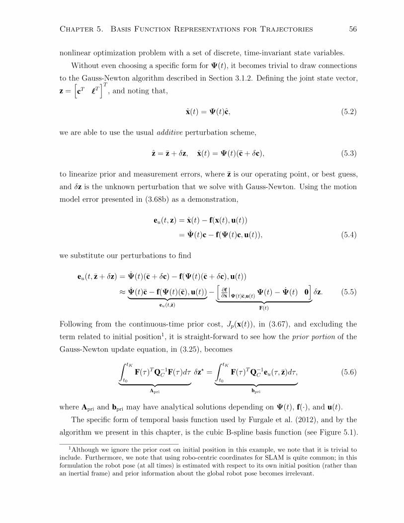
Chapter 5. Basis Function Representations for Trajectories 56
nonlinear optimization problem with a set of discrete, time-invariant state variables.
Without even choosing a specific form for Ψ(t), it becomes trivial to draw connections
to the Gauss-Newton algorithm described in Section 3.1.2. Defining the joint state vector,
z =[cT `T
]T, and noting that,
x(t) = Ψ(t)c, (5.2)
we are able to use the usual additive perturbation scheme,
z = z + δz, x(t) = Ψ(t)(c + δc), (5.3)
to linearize prior and measurement errors, where z is our operating point, or best guess,
and δz is the unknown perturbation that we solve with Gauss-Newton. Using the motion
model error presented in (3.68b) as a demonstration,
eu(t, z) = x(t)− f(x(t),u(t))
= Ψ(t)c− f(Ψ(t)c,u(t)), (5.4)
we substitute our perturbations to find
eu(t, z + δz) = Ψ(t)(c + δc)− f(Ψ(t)(c + δc),u(t))
≈ Ψ(t)c− f(Ψ(t)(c),u(t))︸ ︷︷ ︸eu(t,z)
−[∂f∂x
∣∣Ψ(t)c,u(t)
Ψ(t)− Ψ(t) 0]
︸ ︷︷ ︸F(t)
δz. (5.5)
Following from the continuous-time prior cost, Jp(x(t)), in (3.67), and excluding the
term related to initial position1, it is straight-forward to see how the prior portion of the
Gauss-Newton update equation, in (3.25), becomes∫ tK
t0
F(τ)TQ−1C F(τ)dτ︸ ︷︷ ︸
Apri
δz? =
∫ tK
t0
F(τ)TQ−1C eu(τ, z)dτ,︸ ︷︷ ︸
bpri
(5.6)
where Apri and bpri may have analytical solutions depending on Ψ(t), f(·), and u(t).
The specific form of temporal basis function used by Furgale et al. (2012), and by the
algorithm we present in this chapter, is the cubic B-spline basis function (see Figure 5.1).
1Although we ignore the prior cost on initial position in this example, we note that it is trivial toinclude. Furthermore, we note that using robo-centric coordinates for SLAM is quite common; in thisformulation the robot pose (at all times) is estimated with respect to its own initial position (rather thanan inertial frame) and prior information about the global robot pose becomes irrelevant.

Chapter 5. Basis Function Representations for Trajectories 57
Figure 5.1: This figure illustrates our use of weighted temporal basis functions in one dimension;
the example has nine uniformly spaced cubic B-spline basis functions that are used to define the
weighted sum (black) over six time segments. One can imagine varying the shape of the (black)
sum by scaling the weights (i.e., heights) of the underlying B-splines. A single cubic B-spline is
a smooth piecewise polynomial defined over four time segments; therefore, only four of the basis
functions have a nonzero contribution to the sum at any one query time – this is known as local
support. The points in time that separate two time segments are known as knots.
The use of B-spline basis functions as a parametric representation is common due to
their good representational power, easy analytical derivatives/integrals, and local support
property; local support is desirable to our STEAM framework as it helps to enable
incremental estimation. Using cubic B-splines, with only four basis functions non-zero at
any time, we note that Ψ(t), for the bth time segment, ub ≤ t ≤ ub+1, can be written
Ψ(t) =
ub(t)T B P1,b
...
ub(t)T B Pd,b...
ub(t)T B PD,b
, ub(t) =
1
( t−ubub+1−ub
)
( t−ubub+1−ub
)2
( t−ubub+1−ub
)3
, B =1
6
1 4 1 0
−3 0 3 0
3 −6 3 0
−1 3 −3 1
, (5.7)
where ub(t) is a cubic interpolation function based on the adjacent knot times, ub and
ub+1, B is a fixed coefficient matrix, and Pd,b ∈ R4×(D×B) is a projection matrix that picks
the relevant four coefficients (for dimension d and time segment b) out of state vector c.
In order to parameterize the non-commutative transformations required for 6D pose
estimation, Furgale et al. (2012) chose to directly estimate the Cayley-Gibbs-Rodrigues
axis-angle parameterization, ϕ(t) ∈ R3, and the translation vector, r(t) ∈ R3, such that
T(x(t)) :=
[C(ϕ(t)) r(t)
0T 1
], x(t) :=
[r(t)
ϕ(t)
]= Ψ(t)c, (5.8)
where C(·) and T(·) are mappings to SO(3) and SE(3), respectively. Although this
representation was successful in allowing Furgale et al. (2012) to perform camera/IMU

Chapter 5. Basis Function Representations for Trajectories 58
calibration with a hugely compressed state vector, we note that it is not singularity-free
and far less useful in a free range of motions.
5.3 Relative Coordinate Formulation Using Velocity
In this section, we describe and formulate the relative, continuous-time SLAM problem. To
attain the desirable properties of both the relative and continuous-time SLAM formulations,
it is proposed that the trajectory be represented by the robot velocity, expressed in the
local robot coordinate frame. The intuition behind this decision is derived from the nature
of both the continuous-time and relative formulations. Consider a discrete-time system
in which we sample the robot’s pose at several times and then construct the series of
relative pose changes that make up that trajectory. Now, if we consider reducing that
sampling period to an infinitesimal level, we note that the series of infinitesimal relative
pose changes is in essence the robot-oriented velocity. Recovering a relative pose change
between any two times is simply a matter of integrating the velocity information between
them. Similar to the typical visual SLAM problem, our goal is to find the optimal solution
for the robot trajectory and the map parameters.
5.3.1 Velocity Profile
To define the velocity profile, we begin by introducing the coordinate frames F−→i, our
inertial reference frame, and F−→s(t), the robot’s instantaneous sensor frame. In the
relative, continuous-time formulation of the problem, our algorithm aims to estimate the
generalized six-dimensional (6D) velocity of the robot,
$(t) :=
[νt,it
ωt,it
], (5.9)
which is expressed in the robot’s sensor frame over the time interval t = [0, T ], where νt,it
and ωt,it are the linear and angular components. Note that for simplicity, all references to
the time-varying sensor frame, F−→s(t), have been replaced with the timestamp that we
wish to reference (e.g., time t in the velocity, νt,it ). Notably, an advantage of the velocity
profile trajectory representation (in contrast to using rotations or transformations) is that
there are no constraints that need to be enforced on the parameters of the solution.

Chapter 5. Basis Function Representations for Trajectories 59
5.3.2 Kinematics
In order to include measurements that depend on the pose, or pose change, of the robot,
in a batch estimation scheme, we must first derive the relationship between the robot
velocity, $(t), and the robot pose, T(t), at time t. Following the discussion of rotations
and transformations in Section 3.2.1, we note that the well-known kinematic equation
relating angular velocity to rotation is
Ct,i = ωt,it∧
Ct,i, (5.10)
where (·)∧ is the skew-symmetric operator in (3.35). Recalling the transformation matrix
definition, in (3.36), and expanding the time derivative of ri,tt , we find that
ri,tt = − d
dt(Ct,irt,ii ) = −Ct,irt,ii − Ct,irt,ii = −ωt,it
∧Ct,i(−ri,ti )− Ct,irt,ii = ωt,it
∧ri,tt + νt,it ,
(5.11)
where we define νt,it := −Ct,irt,ii . Substituting our kinematic equations, (5.10) and (5.11),
into the time derivative of the transformation matrix,
Tt,i =
[Ct,i ri,tt0T 0
]=
[ωt,it
∧Ct,i ωt,it
∧ri,tt + νt,it
0T 0
]=
[ωt,it
∧νt,it
0T 0
][Ct,i ri,tt0T 1
], (5.12)
we derive a nonlinear kinematic equation that relates pose change to $(t):
Tt,i = $(t)∧Tt,i. (5.13)
As we are mostly interested in the pose change of the robot between two non-zero times,
ta and tb, we aim to find a general expression involving the matrix Tt,ta . In order to
replace the inertial reference frame, F−→i, in (5.13) with the sensor frame at time ta, F−→s(ta),
we begin with the expression,
Tt,i = Tt,taTta,i, (5.14)
and take the derivative,
Tt,i = Tt,taTta,i + Tt,taTta,i︸ ︷︷ ︸zero
= Tt,taTta,i, (5.15)
noting that Tt,taTta,i is zero due to the fact that Tta,i does not depend on t. By manipulating
(5.13) and (5.15), we find the expected result,
Tt,ta = $(t)∧Tt,ta . (5.16)
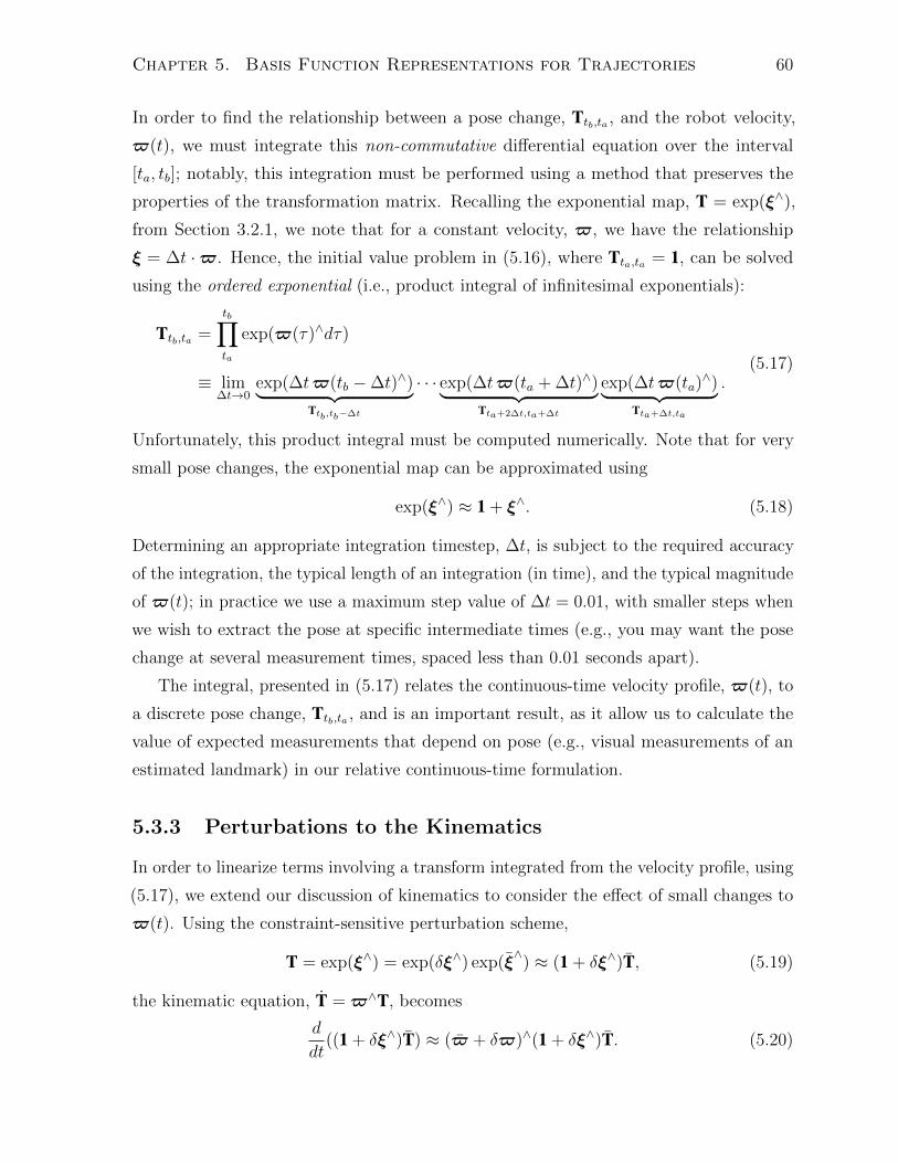
Chapter 5. Basis Function Representations for Trajectories 60
In order to find the relationship between a pose change, Ttb,ta , and the robot velocity,
$(t), we must integrate this non-commutative differential equation over the interval
[ta, tb]; notably, this integration must be performed using a method that preserves the
properties of the transformation matrix. Recalling the exponential map, T = exp(ξ∧),
from Section 3.2.1, we note that for a constant velocity, $, we have the relationship
ξ = ∆t ·$. Hence, the initial value problem in (5.16), where Tta,ta = 1, can be solved
using the ordered exponential (i.e., product integral of infinitesimal exponentials):
Ttb,ta =
tb∏ta
exp($(τ)∧dτ)
≡ lim∆t→0
exp(∆t$(tb −∆t)∧)︸ ︷︷ ︸Ttb,tb−∆t
· · · exp(∆t$(ta + ∆t)∧)︸ ︷︷ ︸Tta+2∆t,ta+∆t
exp(∆t$(ta)∧)︸ ︷︷ ︸
Tta+∆t,ta
.(5.17)
Unfortunately, this product integral must be computed numerically. Note that for very
small pose changes, the exponential map can be approximated using
exp(ξ∧) ≈ 1 + ξ∧. (5.18)
Determining an appropriate integration timestep, ∆t, is subject to the required accuracy
of the integration, the typical length of an integration (in time), and the typical magnitude
of $(t); in practice we use a maximum step value of ∆t = 0.01, with smaller steps when
we wish to extract the pose at specific intermediate times (e.g., you may want the pose
change at several measurement times, spaced less than 0.01 seconds apart).
The integral, presented in (5.17) relates the continuous-time velocity profile, $(t), to
a discrete pose change, Ttb,ta , and is an important result, as it allow us to calculate the
value of expected measurements that depend on pose (e.g., visual measurements of an
estimated landmark) in our relative continuous-time formulation.
5.3.3 Perturbations to the Kinematics
In order to linearize terms involving a transform integrated from the velocity profile, using
(5.17), we extend our discussion of kinematics to consider the effect of small changes to
$(t). Using the constraint-sensitive perturbation scheme,
T = exp(ξ∧) = exp(δξ∧) exp(ξ∧) ≈ (1 + δξ∧)T, (5.19)
the kinematic equation, T = $∧T, becomes
d
dt((1 + δξ∧)T) ≈ ($ + δ$)∧(1 + δξ∧)T. (5.20)

Chapter 5. Basis Function Representations for Trajectories 61
By expanding and dropping small terms, we find
˙T + δξ∧ ˙T + δξ∧
T ≈ $∧T + $∧δξ∧T + δ$∧T. (5.21)
Using the nominal solution, ˙T = $∧T, and the identity, ξ∧1 ξ∧2 −ξ∧2 ξ∧1 ≡ (ξf1 ξ2)∧, equation
(5.21) can be manipulated to find,
δξ∧$∧T + δξ∧
T ≈ $∧δξ∧T + δ$∧T
δξ∧ ≈ −δξ∧$∧ + $∧δξ∧ + δ$∧
= ($fδξ)∧ + δ$∧
δξ ≈ $fδξ + δ$. (5.22)
Giving us the nominal and perturbed equations:
˙T(t) = $(t)∧T(t), (5.23a)
δξ(t) = $(t)fδξ(t) + δ$(t), (5.23b)
which can be integrated separately and combined to provide the full solutions. We have
shown in (5.17) how the nonlinear nominal solution can be integrated numerically. The
perturbed equation is a linear time-varying equation of the form
x(t) = A(t)x(t) + B(t)u(t). (5.24)
The general solution to this initial value problem is given by
x(t) = Φ(t, 0)x(0) +
∫ t
0
Φ(t, τ)B(τ)u(τ)dτ, (5.25)
where Φ(t, τ) is called the state transition matrix and satisfies
Φ(t, τ) = A(t)Φ(t, τ), (5.26a)
Φ(τ, τ) = 1. (5.26b)
The state transition matrix always exists and is unique, but it cannot always be found
analytically. For our particular perturbed equation, we found that it can be expressed as:
Φ(t, τ) = T (t)T (τ)−1. (5.27)
where we recall that T is the adjoint transformation matrix in (3.44). To verify, we check
that (5.27) satisfies the required conditions of a state transition matrix:
Φ(t, τ) =d
dtT (t)T (τ)−1 = ˙T (t)T (τ)−1 = $(t)fT (t)T (τ)−1 = $(t)fΦ(t, τ), (5.28a)
Φ(τ, τ) = T (τ)T (τ)−1 = 1, (5.28b)

Chapter 5. Basis Function Representations for Trajectories 62
where T (t) = $(t)fT (t) is the adjoint version of T(t) = $(t)∧T(t). Using the general
solution to the initial value problem, we have that:
δξ(t) = T (t)T (0)−1δξ(0) + T (t)
∫ t
0
T (τ)−1δ$(τ)dτ. (5.29)
To verify again that this is indeed the correct solution, we can differentiate:
δξ(t) = ˙T (t)T (0)−1δξ(0) + ˙T (t)
∫ t
0
T (τ)−1δ$(τ)dτ + T (t)T (t)−1δ$(t)
= $(t)f(T (t)T (0)−1δξ(0) + T (t)
∫ t
0
T (τ)−1δ$(τ)dτ
)︸ ︷︷ ︸
δξ(t)
+δ$(t)
= $(t)fδξ(t) + δ$(t). (5.30)
We now wish to consider the extension of (5.29) to a general pose change, Ttb,ta , between
two non-zero times, ta and tb. We begin by noting,
Ttb,ta = exp(δξ∧tb,ta)Ttb,ta ≈(1 + δξ∧tb,ta
)Ttb,ta . (5.31)
Using the identity, T exp(w∧) ≡ exp((T w)∧)T, we then derive that,
Ttb,ta = T(tb)T(ta)−1
= exp(δξ(tb)∧)T(tb)
(exp(δξ(ta)
∧)T(ta))−1
= exp(δξ(tb)∧)T(tb)T(ta)
−1 exp(−δξ(ta)∧)
= exp(δξ(tb)∧) exp((−T (tb)T (ta)
−1δξ(ta))∧)Ttb,ta
≈ (1 + δξ(tb)∧)(1− (T (tb)T (ta)
−1δξ(ta))∧) Ttb,ta
≈(1 + (δξ(tb)− T (tb)T (ta)
−1δξ(ta))∧) Ttb,ta . (5.32)
Comparing (5.31) and (5.32), we find the relationship,
δξtb,ta ≈ δξ(tb)− T (tb)T (ta)−1δξ(ta). (5.33)
To simplify the term δξ(tb) − T (tb)T (ta)−1δξ(ta), and relate the perturbation back to
our velocity profile, $(t), we substitute the solution for δξ(t) found in (5.29):
δξ(tb)− T (tb)T (ta)−1δξ(ta) =
(T (tb)T (0)−1δξ(0) + T (tb)
∫ tb
0
T (τ)−1δ$(τ)dτ
)−T (tb)T (ta)
−1
(T (ta)T (0)−1δξ(0) + T (ta)
∫ ta
0
T (τ)−1δ$(τ)dτ
)= T (tb)
(∫ tb
0
T (τ)−1δ$(τ)dτ −∫ ta
0
T (τ)−1δ$(τ)dτ
)=
∫ tb
ta
T tb,τ δ$(τ)dτ. (5.34)

Chapter 5. Basis Function Representations for Trajectories 63
Substituting (5.34) back into (5.31), we find the following relationship between Ttb,ta and
small changes in $(t),
Ttb,ta ≈(
1 +
(∫ tb
ta
T tb,τ δ$(τ)dτ
)∧)Ttb,ta . (5.35)
Although it is initially unclear how one might isolate the time-varying parameter, δ$(t),
since it is embedded in the integral, the following section will show how this is made
manageable with the use of parametric basis functions.
The relationship in (5.35) between a pose change, Ttb,ta , and a perturbation to the
velocity profile, δ$(t), allows us to use this relative continuous-time formulation with
the Gauss-Newton optimization technique described in Section 3.1.2. The nominal pose
change, Ttb,ta , is integrated from the nominal velocity profile, $(t), using (5.17).
5.3.4 Parametric Batch Estimator
Trajectory Parameterization
In the relative, continuous-time formulation of the SLAM problem, we wish to estimate
the 6D velocity of the robot, $(t), which is expressed in the robot’s sensor frame, over the
time interval t = [t0, tK ]. Moving forward in the derivation of the estimator, we define a
parametric representation for the continuous-time state. Similar to the method described
in Section 5.2, we use a weighted sum of temporal basis functions,
$(t) := Ψ(t)c, Ψ(t) :=[ψ1(t) ψ2(t) · · · ψ6B(t)
], (5.36)
where we have B temporal basis functions in each of the six problem dimensions, and
each basis function, ψb(t), is a 6× 1 column vector. The coefficients (i.e., state variables),
c ∈ R6B, can be used to vary the velocity estimate,$(t); using a parametric representation,
the estimation goal is to simply find the optimal values of these weights.
Owing to the requirement that our basis functions have local support, which will
be discussed later, our implementation uses cubic B-spline basis functions (as seen in
Figure 5.1); note our method is not tied to using only cubic B-splines – any basis function
that exhibits local support is satisfactory.
Loop Closures
In addition to the relative trajectory, we also wish to estimate any loop-closure transfor-
mations between segments of the trajectory from distinctly different times. These loop

Chapter 5. Basis Function Representations for Trajectories 64
closures are stored as 4× 4 homogeneous transformation matrices,
TLCt2,t1
:= T(t2)T(t1)−1, (5.37)
between the sensor frame, F−→s(t), at the two distinct times, t1 and t2. As described in
Section 3.3.2, these loop-closure transformations over-parameterize the trajectory solution
provided by $(t), but allow us to perform loop-closure optimizations using a window-style
filter; these optimizations are constant time and generate locally accurate maps.
Landmarks
To complete the traditional SLAM state formulation, we also estimate the positions of the
landmark parameters, `j. The landmarks are stored using homogeneous coordinates, as
described in Section 3.2.2. Adopting the relative formulation of SLAM (with no privileged
coordinates frames), it becomes important that each landmark position is stored locally;
this is implemented by expressing, `j, in frame F−→s(tj), the sensor pose at time tj,
p`j ,tjtj :=
[`j
1
]∈ R4, `j = P`,j`, (5.38)
where we define tj to be the first measurement time of the jth landmark, and P`,j is a
projection matrix that selects the 3D position `j from the state vector `. In order to
simplify the notation, we also denote tk := tkj, the time of measurement ykj.
Optimization Problem
The joint state that we wish to estimate is defined as z := θ, `, where the state θ
contains parameters related to robot pose, and ` is the vector of landmark positions. In
the open-loop case, θ := c; however, if a loop closure is part of the optimization problem,
then θ := c,TLCt2,t1. Recalling the standard SLAM/STEAM formulations, it follows that
our measurement and prior objective functions are
Jm(z) :=1
2
∑kj
eTmkjR−1kj emkj , Jp(c) :=
1
2
∫ T
t=0
eu(τ)TQ−1eu(τ)dτ, (5.39)
where Jm is a cost associated with the landmark measurements, and Jp is a cost associated
with motion (i.e., a motion prior). Note that Jp does not include a prior term related to
initial position; our initial uncertainty is zero because all (relative) estimates are performed
with respect to the robocentric frame. Also, we note that loop-closure constraints are

Chapter 5. Basis Function Representations for Trajectories 65
Closed-Loop Patht2
t1
Open-Loop PathT ,t2
TLCt2,t1
Tt1,
j tk
tj tj
tk
Figure 5.2: In order to formulate an expected measurement, gkj(z), the point `j , which is
expressed in the sensor frame at time tj , needs to be transformed to the current observation
time, tk. In the general open-loop case (seen in blue), the transform, Ttk,tj , is found by simply
integrating the continuous-time velocity profile. However, the existence of loop closures create
alternate integration paths (seen in red). Integration of the shortest temporal path is often the
most desirable, as it incurs the least estimation error.
introduced in the estimation problem solely through the landmarks that are observed
from both of the matched trajectory segments, as discussed in the next subsection.
Cost Terms
Recalling the nonlinear observation error from (3.10), and the camera model example
from (3.58), we formulate our measurement errors as
emkj(z) = ykj − gkj(z), gkj(z) := k(hkj(z)), hkj(z) = Ttk,tj p`j ,tjtj (5.40)
where ykj is our measurement, gkj(·) is the general nonlinear observation model, k(·) is a
nonlinear camera model, hkj(·) is the transformed homogeneous coordinate, Ttk,tj is the
4× 4 homogeneous transform matrix that specifies the pose change in the sensor frame
between the measurement times tj and tk, and p`j ,tjtj is the position of relative landmark
`j in homogeneous coordinates. For our experimental results, using lidar, we model k(·)as the spherical camera model presented in Appendix Section A.2.
To evaluate this cost using the velocity profile, $(t), we note that in the open-loop
case, the unknown transforms, Ttk,tj , are found by simply integrating over the continuous-
time velocity profile. However, in the case that the shortest temporal path between tj and
tk involves a loop closure, we note that Ttk,tj becomes the composition of the following
transformation matrices,
Ttk,tj = Ttk,t2TLCt2,t1
Tt1,tj , (5.41)
where Ttk,t2 and Tt1,tj are integrated using the velocity profile, and TLCt2,t1
exists as a
discrete loop-closure transformation between times t1 and t2. These alternate integration
paths are illustrated in Figure 5.2.

Chapter 5. Basis Function Representations for Trajectories 66
Assuming no knowledge of the control signal, we model the motion as a zero-mean
white noise on acceleration. This can be written as the Gaussian process
eu(t) := $(t) = w(t), w(t) ∼ GP(0,QCδ(t− t′)), (5.42)
where QC is the power-spectral-density matrix and δ(·) is Dirac’s delta function.
Using the Kinematic Perturbation
In order to minimize J(z) using our standard Gauss-Newton approach, we first make
it quadratic in a small perturbation of the state, δz :=[δθT δ`T
]T, and then find the
optimal state update δz? by solving ∂T J∂δz = 0; in the open-loop case, δθ := δc, and in the
closed-loop case, δθ :=[δcT δξLC
t2,t1
T]T
. We note that the linearization of Jp takes the
same approach as Furgale et al. (2012), described in Section 5.2, and therefore this section
will focus only on the linearization of Jm.
From the temporal basis function definition, $(t) := Ψ(t)c, we can define an additive
perturbation model, $(t) = $(t) + δ$(t), such that $(t) + δ$(t) = Ψ(t)(c + δc), and
therefore δ$(t) = Ψ(t)δc. Substituting this relationship into (5.35), we find that
Ttb,ta ≈(
1 +
(∫ tb
ta
T tb,τΨ(τ)dτ δc)∧)
Ttb,ta , (5.43)
and therefore our usual perturbation, δξtb,ta , to transform Ttb,ta , is
δξtb,ta ≈(∫ tb
ta
T tb,τΨ(τ)dτ
)δc. (5.44)
Recalling the example camera model linearization in (3.63), we apply our constraint-
sensitive perturbations to an open-loop trajectory integration to find that
emkj(z + δz) = ykj − k(Ttk,tj p`j ,tjtj )−Gkjδz, (5.45)
Gkj :=[KkjHx,kjHc,kj KkjH`,kjP`,j
], (5.46)
where Kkj, Hx,kj, and H`,kj were defined in (3.62) and (3.64), and from (5.44) we have
Hc,kj :=
∫ tk
tj
T tk,τΨ(τ)dτ. (5.47)
Note that when a loop closure is present in the shortest pose chain from tj to tk (i.e.,
Ttk,tj = Ttk,t2TLCt2,t1
Tt1,tj), the formulation changes slightly. Using the same perturbation
scheme, with the additional perturbation δξLCt2,t1
, it is straightforward to show that
Gkj :=[KkjHx,kjHc,kj KkjHx,kjT tk,t2 KkjH`,kjP`,j
], (5.48)

Chapter 5. Basis Function Representations for Trajectories 67
where δz =[δcT δξLC
t2,t1
Tδ`T]T
, and
Hc,kj :=
(∫ tk
t2
T tk,τΨ(τ)dτ +
∫ t1
tj
T tk,τΨ(τ)dτ
). (5.49)
Gauss-Newton Algorithm
Finally, connecting our state representation, cost terms, and Jacobians to the Gauss-
Newton update equation in (3.25), we have that
(Ameas + Apri) δz? = bmeas + bpri. (5.50)
where
Ameas :=∑kj
GTkjR
−1kj Gkj, bmeas :=
∑kj
GTkjR
−1kj emkj(z), (5.51)
and it follows from (5.6) and (5.42) that
Apri :=
[∫ T0
Ψ(τ)TQ−1C Ψ(τ) dτ 0
0 0
], bpri := −Apriz. (5.52)
Note that the term Apri only needs to be calculated once, as it does not depend on the
state parameters. Following the Gauss-Newton approach, the solution to δz? is used
to update the nominal solutions iteratively and to convergence. The pertinent state
update equations are: c ← c + δc?, ¯ ← ¯ + δ`?, and in the case of a loop closure,
TLCt2,t1← exp((δξLCt2,t1
?)∧)TLC
t2,t1.
Implementation Efficiency
There are three major computational costs associated with running this estimator. The
first major cost is the numerical integrations of (5.17) and (5.47). We note from the
derivation of (5.34) that the integral term in Hc,kj can be written as∫ tk
tj
T tk,τΨ(τ)dτ = Ad(T(tk))(I(tk)− I(tj)), (5.53)
where,
I(t) :=
∫ t
0
Ad(T(τ))−1Ψ(τ)dτ. (5.54)

Chapter 5. Basis Function Representations for Trajectories 68
Given that many of the required integral calculations will overlap, we aim to compute all
the integral terms efficiently by conducting a single pass over the entire time period that
we are currently optimizing. In the full batch optimization, the following equations are
used iteratively for t = [t0, tK ],
T(t+ ∆t)← exp ((∆t ·Ψ(t)c)∧) T(t), (5.55a)
I(t+ ∆t)← I(t) + ∆t · Ad(T(t))−1Ψ(t), (5.55b)
where T(0) = 1 and I(0) = 0. The integration step, ∆t, is chosen so that we have
intermediate terms for T and I at each measurement time, tkj. By storing the intermediate
steps, we can compute Ttk,tj and Gkj for each measurement.
The second major cost in this estimator is building the matrix Ameas. This step can be
exceptionally expensive depending on the choice of basis functions used to parameterize
Ψ(t). Specifically, it is highly beneficial to use a basis function type that has local support.
At any given time, we want only a subset of the basis functions, ψb(t), to be non-zero.
Using local support introduces an exploitable sparsity to the matrix Ψ(t). As mentioned
in Section 5.3.4, our implementation of the estimator uses cubic B-spline basis functions,
because they have local support in addition to simple analytical integrals and derivatives.
The third cost is related to solving the linear system of equations in (5.50). To do
this efficiently, we note that it can be written using the 2× 2 block structure,[Axx Ax`
ATx` A``
][δθ?
δ`?
]=
[bxb`
]. (5.56)
Notably, the relative, continuous-time formulation of the problem changes the traditional
sparsity pattern of Axx; this is due to the fact that Apri is now band diagonal, and the
relative transforms, Ttk,tj , may depend on long strides of temporally related state variables
in c, and sometimes loop closures, TLCt2,t1
. However, since A`` is still block-diagonal and is
typically much larger than Axx, we may apply the usual Schur complement, discussed in
Section 3.1.3, with no additional cost.
B-spline Window Filter
Here we describe our continuous-time approach to the incremental optimization method-
ology discussed in Section 3.3.2. In order to run the estimator online we optimize over
a subset of the basis functions used in the time segments leading up to the most recent
measurement. However, in order for this technique to achieve constant-time performance,

Chapter 5. Basis Function Representations for Trajectories 69
Active Time Segments
Part of the Active StatePart of the Static State
Integration
j+2+1j
1j j
Figure 5.3: This figure depicts the use of active state parameters in a window-style filter. For
illustration, uniformly weighted cubic B-spline basis functions are used to portray the parametric
velocity profile estimate. The integrated robot trajectory, shown above the velocity profile, is
depicted to align on the time axis, with the landmarks observed at the connected timestamps.
Determining the active state begins by defining the active time segments; any basis function
that influences the active time segments becomes part of the active state. Landmark variables
are considered active if they are observed from a time that overlaps with an active basis function.
The static region is required to calculate expected measurements for landmarks with observations
from both active and static time intervals (e.g., `j).
the subset of basis functions must have temporally local effects on the robot trajectory,
$(t). For this to be true, it is a requirement that the basis functions used in the estimator
have local support.
Before setting up the local batch optimization problem, we begin by identifying the
active state, illustrated in Figure 5.3. The active subset of basis functions and all landmarks
measured during the affected time period are added to a list of active parameters that will
be updated in the optimization. All measurements of these active landmark parameters
are included when building the terms Ameas and bmeas. This may require the full nominal
solution, c, as some of the static basis function coefficients may be required to evaluate
$(t) near and outside the bounds of the active time period.
In the case of a loop closure, the active state selection changes slightly to include both
the discrete loop-closure transformation and the temporal basis functions on both sides
of the spatial link; the basis functions that are made active are the ones that overlap in
time with any of the landmark observations that were matched across the loop closure.
Pose-Graph Relaxation
Although the relative SLAM problem formulation argues that a global map is not necessary
for many common robotic tasks, a global map may be desirable or required in some

Chapter 5. Basis Function Representations for Trajectories 70
situations; for example, human inspection of a large-scale map, or human-in-the-loop
decisions, such as macro-level path planning or goal setting.
In order to generate a globally consistent SLAM solution in a computationally tractable
manner, a common practice is to implement pose-graph relaxation or pose-graph SLAM ;
the derivation of which is well known (Olson et al., 2006; Grisetti et al., 2007). The general
concept of the optimization is to use the estimated discrete relative pose transforms as
measurements in a new problem that aims to solve for the global poses.
To relax the relative continuous-time trajectory into global coordinates, we first
discretize our solution into a set of relative transforms, Ttd+1,td , which occur between
times td and td+1, for d = 1 . . . D. Obtaining the relative transforms is straightforward
using the integration scheme in (5.17),
Ttd+1,td = T(td+1)T(td)−1 =
td+1∏td
exp($(τ)∧dτ). (5.57)
However, obtaining the uncertainty of the relative pose estimates,
Σd+1,d := E[δξtd+1,tdδξTtd+1,td
], (5.58)
involves some additional derivation. Note that the result from Barfoot and Furgale (2014)
on compounding poses using fourth-order terms is not directly applicable to finding the
uncertainty of the transform, Ttd+1,td , because δξ(td) and δξ(td+1) are correlated.
Using the relationship in (5.35) it is straightforward to see that
δξtd+1,td≈(T (td+1)
∫ td+1
td
T (τ)−1δ$(τ)dτ
), (5.59)
and therefore,
Σtd+1,td =E[δξtd+1,td
δξTtd+1,td
]≈E[(
T (td+1)
∫ td+1
td
T (τ)−1δ$(τ)dτ
)(T (td+1)
∫ td+1
td
T (τ ′)−1δ$(τ ′)dτ ′)T]
=T (td+1)
∫ td+1
td
∫ td+1
td
T (τ)−1E[δ$(τ)δ$(τ ′)T
]T (τ ′)−Tdτ ′dτ T (td+1)T . (5.60)
In practice, because we have parameterized the solution using basis functions, δ$(t) =
Ψ(t)δc, it is convenient to compute the covariance as follows,
Σtd+1,td ≈(T (td+1)
∫ td+1
td
T (τ)−1Ψ(τ)dτ
)E[δc δcT
](T (td+1)
∫ td+1
td
T (τ ′)−1Ψ(τ ′)dτ ′)T
,
(5.61)

Chapter 5. Basis Function Representations for Trajectories 71
LargeLoop
Root
Local Region
Integrated Estimate
Ground Truth
Figure 5.4: Illustration of the local RMS error calculation for a single root node. Note that
open-loop integration (OLI) outside of the local region is needed to find the top two poses, while
closed-loop integration (CLI) can be used to quickly find the lower poses.
where E[δc δcT ] can be evaluated using part of the solution from our Gauss-Newton
optimization problem in (5.50), after convergence. Using the Schur complement for an
open-loop optimization, we know that
cov(δθ?, δθ?) = E[δc? δc?T
]= (Axx − Ax`A−1
`` ATx`)−1, (5.62)
and in a closed-loop optimization,
cov(δθ?, δθ?) =
E[δc? δc?T
]E[δc? δξLCt2,t1
?T]
E[δξLCt2,t1
?δc?T
]E[δξLCt2,t1
?δξLCt2,t1
?T]= (Axx − Ax`A−1
`` ATx`)−1, (5.63)
where E[δξLCt2,t1
?δξLCt2,t1
?T]
is the uncertainty associated with TLCt2,t1
.
5.3.5 Appearance-Based Lidar Experiment
In this section, we test and report results for our relative continuous-time SLAM technique.
The estimator is tested using a set of real data that highlight our algorithm’s ability
to handle high-rate asynchronous measurements, while the robot undergoes motion in
unstructured terrain. The 1.1km traversal, measurements models, and place recognition,
are described in Appendix A.
Local Accuracy Metric
Before discussing the results of the estimator, we begin by introducing the average local-
area root-mean-square (ALARMS) error, a new metric similar to the one introduced by
Sibley et al. (2010), which we use to evaluate local metric accuracy. The ALARMS error
calculation is illustrated in Figure 5.4, and proceeds as follows:

Chapter 5. Basis Function Representations for Trajectories 72
For each ground-truth node,
1. Search the ground truth (GPS) for all other nodes within some specified distance of
the current (root) node – this is our local region
2. Perform a breadth first search (BFS) using the available topological information,
starting with the root node, to determine the shortest paths to all other local nodes
3. Integrate along the found paths to obtain the pose of local nodes in the root node’s
coordinate frame
4. Fix the root node’s pose to ground truth; in the absence of global orientation
information, align the trajectories using all the integrated local node positions and
ground truth counterparts
5. Compute RMS Euclidean error for the local region subgraph
The ALARMS error is then the average of all the calculated RMS errors terms, where
each error term is generated by using one of the ground-truth nodes to form a local
region. In the absence of loop closures, only temporal links contribute to the topological
connectivity of the graph.
The purpose of this error metric is to evaluate the local (rather than global) metric
accuracy of an algorithm. Enforcing a globally consistent solution (e.g., via pose-graph
relaxation) before comparing to ground-truth prevents us from gaining insight to an
algorithm’s local accuracy. The ALARMS error metric evaluates accuracy within a fixed-
size region (averaged over ‘all of the regions’); by then varying the region size we can
analyze the performance of an algorithm over different scales.
Open-Loop Solution
Processing the 6880 intensity images (in a VO-style fashion), we found 2,010,671 temporally
matched SURF feature measurements, each with a unique timestamp. Assuming the
use of a (brute-force) discrete-time batch estimator (with a motion prior), the state
parameterization would require a pose estimate at each measurement time in the system;
meaning that for the 1.1km dataset, it would naively require 6 × 2,010,671 = 12,064,026
state variables, excluding the 688,481 different landmark positions. Furthermore, the
plain discrete-time solution is ill-conditioned without a motion prior and cannot be solved.
Using basis functions to parameterize our continuous-time state, we show how the number
of required state variables can be drastically reduced.

Chapter 5. Basis Function Representations for Trajectories 73
Direction Switch
(a) Velocity Profile
Direction Switch
Start
(b) Integrated Trajectory
Figure 5.5: Example output from the relative continuous-time SLAM estimator using real
data. The linear and angular velocity estimates in (a) directly correspond to the integrated 3D
trajectory in (b); coordinate frames are plotted at a uniform time interval. The direction switch
in forward (x) velocity can be easily observed in the integrated trajectory.
Before running the constant-time estimator on the entire 1.1km trajectory, we must
decide on a spacing for the temporal basis functions and an appropriate window size over
which to optimize. In order to train these two parameters, we use a 250m subsection of
the full trajectory. To compare the results of the estimator to the GPS ground truth, we
consider the integral of our velocity estimate, as seen in Figure 5.5.
To find an appropriate knot spacing, we iterated the full batch estimator on the
training section, varying the number of time segments in the B-spline parameterization
from 5 to 3000. The accuracy of the solutions are quantified by considering both the
total root-mean-square (RMS) Euclidean error, comparing the integrated position of our
velocity estimate to the DGPS tracks, and the ALARMS error, for a 10 metre local region.
The estimate and DGPS tracks were put into a common reference frame by aligning the
first 10 meters of each trajectory.
The result of varying the number of knots can be seen in Figure 5.6 (timing was broken
down into the three major steps described in Section 5.3.4). Using the efficient methods
described earlier, we see that the integration and build steps of the algorithm are relatively
constant in cost as the number of knots increases. As expected, the solution to Aδz? = bis cubic in complexity and begins to take a larger portion of the total time as the number
of basis functions is increased. As the knot spacing is reduced, the parameterization is
given enough degrees of freedom to properly represent the velocity profile of the robot;
however, there are diminishing returns with respect to reducing error. For this subsection
of the dataset, it was decided that 1200 time segments (a knot spacing of approximately

Chapter 5. Basis Function Representations for Trajectories 74
Chosen basis function spacing
Figure 5.6: The full batch estimator was run
on a 250m subsection of the full dataset. Vary-
ing the number of time segments in the pa-
rameterization from 5 to 3000, we aim to find
an appropriate knot spacing to use over the
entire trajectory. The chosen number of time
segments was 1200 (a knot spacing of approxi-
mately 0.65 seconds).
Chosen window size
Figure 5.7: Using 1200 time segments in the B-
spline parametrization over the 250m training
segment, we varied the number of active time
segments in each optimization window from 1
to 20. The chosen optimization window size
for the final experiment was 5 time segments.
The compute time is the average time it took
to compute a single window optimization.
0.65 seconds) was acceptable to represent the robot trajectory.
In order to limit the growth rate in solve time, we applied our window-style filter
to the 250m trajectory. In a similar fashion to the first experiment, we then varied the
number of active time segments in the optimization window from 1 to 20. The results
in Figure 5.7 indicate that a window size of only 5 time segments would be sufficient to
use over the entire trajectory. The compute time shown in this experiment is the average
amount of time taken to solve a single window optimization. Increasing window size has
a clear negative effect on the amount of time spent integrating and building the terms
needed in the solution.
The final result for the full trajectory estimate, seen in Figure 5.8, is compared
to a discrete-time relative bundle adjustment implementation. To keep the discrete
implementation’s state size tractable and solvable, a single relative pose estimate is used
for each of the image stacks and the laser scans are assumed to be taken instantaneously
(i.e., no motion distortion). The open-loop integration (OLI) of our velocity estimate
and discrete relative bundle adjustment solution are put into a common reference frame

Chapter 5. Basis Function Representations for Trajectories 75
Start/End Start/End
Figure 5.8: Top and side views of the robot trajectory over the whole 1.1km dataset. Our
Relative CT estimator used a knot spacing of 0.65 seconds, and an active window size of 5 time
segments. The relative discrete-time solution used an active window size of 6 images. DGPS
tracks are in black, the discrete-time relative bundle adjustment solution is in red, and the
open-loop integration (OLI) of the velocity profile estimate is in blue. Note the significant
improvement made by properly accounting for the temporal nature of the lidar measurements.
with the DGPS tracks by aligning the first 30 meters of each trajectory. Compensating
for motion distortion by using our continuous-time estimation scheme clearly produces
superior results in contrast to the traditional discrete-time approach.
As suggested by the results of the first experiment, the estimator used a knot spacing
of 0.65 seconds. This correlated to the use of only 6 × 5,386 = 32,316 state variables in
the parameterization of $(t). In relation to the second experiment, it was decided that
the estimator should use a window size of 5 active time segments; this cost approximately
1.3 seconds per local batch optimization and led to a total run time of 1.6 hours2.
Closed-Loop Solution
Using the visual place-recognition algorithm proposed by MacTavish and Barfoot (2014),
followed by geometric verification, we were able to detect nine loop-closure locations
(discussed in Appendix A.3). An optimization was then performed around each loop-
closure for the spatial transformation and the basis functions overlapping in time with
spatially matched landmark observations. In order to see how merging landmarks across
loop closures improves the open-loop estimate, the solution is integrated using both an
OLI and closed-loop integration (CLI) scheme.
Figure 5.9 shows the trajectory integrations for two 20 metre local regions, selected as
part of ALARMS error calculations, which included loop closures. The first region, in
2Implemented in Matlab and timed with a 2.4GHz processor and 8GB of 1333MHz DDR3 RAM.

Chapter 5. Basis Function Representations for Trajectories 76
Local RegionNote how closely the final solution (green)
follows the GPS
(a) Region 1
Local Region
Note how closely the final solution (green)
follows the GPS
(b) Region 2
Figure 5.9: These figures show the trajectory integrations for ALARMS error calculations in
two different areas; each calculation used a 20 m local region size and included a loop closure.
The first region, shown in (a), is near the start/end of the 1.1km trajectory and contains a loop
closure connecting the two trajectory segments. An incremental performance increase is clearly
visible, with the final solution being very near the GPS ground truth. The second region, shown
in (b), includes three trajectory segments, two of which are connected by a loop closure that
spans nearly 200 m. Again, an incremental performance increase is clearly visible.
Figure 5.9(a), includes two trajectory segments, which contain the start and end of the
1.1km traversal. The second region, in Figure 5.9(b), includes three trajectory segments,
two of which are connected by a loop closure that spans roughly 200m. Descriptions of
the algorithms and the resultant RMS error for each region is shown in Table 5.1.
As expected, the discrete algorithm configuration, which does not consider motion
distortion, performs poorly in comparison to all of the continuous-time solutions. Note that
the integration of the trajectory in the second region included less open-loop distance, and
therefore it is expected that the magnitude of errors in the results would be smaller. The
expected reduction in error between the open-loop integrations of the relative continuous-
time trajectory, with and without loop closure, is fairly minimal. In the first region, we
see a fairly substantial improvement, which can be attributed to the small incremental
improvements over the very long open-loop integration distance. In the second region,

Chapter 5. Basis Function Representations for Trajectories 77
Table 5.1: This table describes the different algorithm configurations that will be contrasted
for local accuracy. The two estimators are the Discrete estimator, that assumes no motion
distortion, and the Relative CT estimator using basis function on body-centric velocity. All
configurations use the feature correspondences provided by the motion-compensated RANSAC
algorithm presented in Chapter 4. The final two configurations take advantage of loop closure
information provided by the place-recognition algorithm, but are integrated in different fashions;
one using open-loop integration (OLI) and one using closed-loop integration (CLI). Finally,
RMS errors are shown for the trajectory integrations investigated in Figure 5.9.
Label Loop
Closures
Integration
Scheme
Region 1 RMS
Err. [m]
Region 2 RMS
Err. [m]
Discrete No OLI 13.95 6.32
Rel. CT No OLI 8.61 2.83
Rel. CT w/ LC (OLI) Yes OLI 4.41 2.89
Rel. CT w/ LC (CLI) Yes CLI 0.40 1.14
there is a slight increase in measured error; although it is possible that the additional
measurements and fusion of landmarks reduced the accuracy of the estimation, it must
be considered that the circular error probability (CEP) of our GPS is only 0.4m in the
horizontal plane. Furthermore, this CEP is reported under ideal conditions and the
vertical dimension is typically worst. Finally, we note the solution using CLI in the second
region had more than double the error of the first region for a trajectory of similar size; if
we consider only the two pieces of trajectory tied by loop closure in the second region,
we find the RMS error of the final solution is only 0.44m, giving some insight to the
importance of place recognition for increasing local estimation accuracy. We contrast
the various algorithm configurations more broadly, over the full 1.1km trajectory, by
comparing the ALARMS error for varying local region sizes, as seen in Figure 5.10. Lastly,
we note that the number of available loop closures in this dataset was fairly low, but that
the algorithm should scale well with additional loop closures; Sibley et al. (2010) show in
their discrete-time relative bundle adjustment algorithm that the addition of many loop
closures significantly reduces mapping error, even before global relaxation.
In an offline process, we discretized the continuous-time trajectory, solved for the
covariance of the relative transforms, and performed pose-graph relaxation using the nine
optimized loop closures. The resulting globally consistent trajectory estimate can be seen
in Figure 5.11. While a globally consistent map of this quality is useful for tasks such as
macro-level path planning, or low-frequency human-in-the-loop decisions, we reiterate
that the strength of the relative formulation is a constant-time, locally accurate solution
aimed at enabling autonomous tasks, such as navigation or object avoidance.

Chapter 5. Basis Function Representations for Trajectories 78
Figure 5.10: This figure shows ALARMS error
for a number of local region sizes, using trajec-
tory estimates of the entire 1.1km trajectory.
Note the estimation error drift for continuous-
time solutions is far lower than that of the
discrete solution. Furthermore, the addition
of loop closure improves both the open-loop
and closed-loop results.
Figure 5.11: This figure shows the globally
consistent trajectory estimate generated by dis-
cretizing the full 1.1km continuous-time trajec-
tory, and performing a pose-graph relaxation
using the nine available loop closures. The
RMS error for the full trajectory is 2.9m. If
we consider only the x-y plane, then the RMS
error is 0.77m over the full 1.1km path.
From a navigational standpoint, the ability to close loops in constant time and
generate highly accurate local maps is significant; especially with the growing popularity
of techniques that aim to localize against previously traversed paths in order to repeat
routes (Furgale and Barfoot, 2010; Churchill and Newman, 2012).
5.4 Discussion
The relative, parametric approach to STEAM described in this chapter provided good
estimation accuracy and exhibits the properties that we wish to have in our ideal localiza-
tion engine. However, the estimator performs much more slowly than would be hoped.
The core issue being that we require numerical integration of the velocity profile to form
expected measurements and Jacobians. Furthermore, the fully relative solution also adds
a severe amount of density to the problem; while the general complexity is unaffected
(using the Schur complement), the secondary sparsity is very poor.
The major issue that needs to be addressed in the parametric approach is the algorithm
that determines the knot spacing. In this thesis, we made use of a uniform spacing that
needed to be trained prior to the experiment; in general, this is not desirable. Although
the knot-space training in Figure 5.6 would have us believe that it is safe to simply choose
a very fine knot spacing, further experimentation has shown us both ends of the spectrum
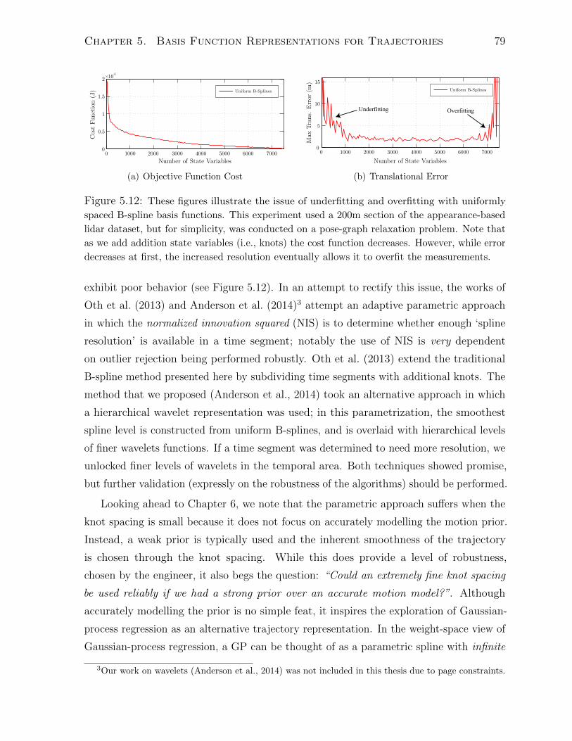
Chapter 5. Basis Function Representations for Trajectories 79
(a) Objective Function Cost
OverfittingUnderfitting
(b) Translational Error
Figure 5.12: These figures illustrate the issue of underfitting and overfitting with uniformly
spaced B-spline basis functions. This experiment used a 200m section of the appearance-based
lidar dataset, but for simplicity, was conducted on a pose-graph relaxation problem. Note that
as we add addition state variables (i.e., knots) the cost function decreases. However, while error
decreases at first, the increased resolution eventually allows it to overfit the measurements.
exhibit poor behavior (see Figure 5.12). In an attempt to rectify this issue, the works of
Oth et al. (2013) and Anderson et al. (2014)3 attempt an adaptive parametric approach
in which the normalized innovation squared (NIS) is to determine whether enough ‘spline
resolution’ is available in a time segment; notably the use of NIS is very dependent
on outlier rejection being performed robustly. Oth et al. (2013) extend the traditional
B-spline method presented here by subdividing time segments with additional knots. The
method that we proposed (Anderson et al., 2014) took an alternative approach in which
a hierarchical wavelet representation was used; in this parametrization, the smoothest
spline level is constructed from uniform B-splines, and is overlaid with hierarchical levels
of finer wavelets functions. If a time segment was determined to need more resolution, we
unlocked finer levels of wavelets in the temporal area. Both techniques showed promise,
but further validation (expressly on the robustness of the algorithms) should be performed.
Looking ahead to Chapter 6, we note that the parametric approach suffers when the
knot spacing is small because it does not focus on accurately modelling the motion prior.
Instead, a weak prior is typically used and the inherent smoothness of the trajectory
is chosen through the knot spacing. While this does provide a level of robustness,
chosen by the engineer, it also begs the question: “Could an extremely fine knot spacing
be used reliably if we had a strong prior over an accurate motion model?”. Although
accurately modelling the prior is no simple feat, it inspires the exploration of Gaussian-
process regression as an alternative trajectory representation. In the weight-space view of
Gaussian-process regression, a GP can be thought of as a parametric spline with infinite
3Our work on wavelets (Anderson et al., 2014) was not included in this thesis due to page constraints.

Chapter 5. Basis Function Representations for Trajectories 80
temporal basis functions – the solution is constrained by putting much more focus on
modelling a strong prior distribution.
5.5 Summary and Conclusions
In this chapter we have presented a batch, parametric, relative, singularity-free, and
continuous-time SLAM estimator that is able to find an incremental approximation to
the MAP problem in constant-time. The estimator presented in this chapter adopts
the completely relative problem formulation by Sibley et al. (2009). However, as the
proposed relative method is also a continuous-time solution, it maintains the ability to
overcome the state-size tractability issues associated with high-rate and scanning sensors
by using the parametric framework derived by Furgale et al. (2012). To attain this fusion
of techniques, the open-loop trajectory is represented by a continuous-time estimate of the
robot’s velocity, while large-scale loop closures are described by discrete transformations
that relate the robot’s pose at two different times. The algorithm was validated using a
1.1 kilometer dataset of motion-distorted lidar intensity imagery. Using this dataset, we
demonstrate that our algorithm is able to compensate for motion-distortion and provide
odometry results much more suitable to navigation than a discrete-time counterpart. The
methods and results presented in this chapter were initially published without loop-closure
results, by Anderson and Barfoot (2013b), and then fully by Anderson et al. (2015b).
In summary, the contributions of this chapter are:
1. A continuous-time adaptation of the relative-coordinate formulation of SLAM. We
demonstrate that by estimating the velocity profile of the robot, we can devise an
incremental SLAM solution that runs in constant time – even at loop closure.
2. An explanation of how to perform sliding-window-style estimation with basis func-
tions that have a local support greater than two.
3. An evaluation of the algorithm using lidar-style VO and appearance-based place
recognition over a 1.1 kilometer traverse of unstructured, three-dimensional terrain.
This work was an important step towards developing real-time continuous-time solu-
tions on the relative pose manifold. In particular, the knowledge we acquired from the
derivations and experiments presented in this chapter greatly influenced the approach of
our (final) GP-based algorithm (presented at the end of Chapter 6).

Chapter 6
Gaussian-Process Representations
for Trajectories
In this chapter we explore novel extensions of the Gaussian-process (GP) regression
approach to batch continuous-time trajectory estimation. The approach, first introduced
by Tong et al. (2012, 2013), directly models the robot trajectory as a one-dimensional GP
(where time is the independent variable) and uses batch estimation to solve for the robot
state at the measurement times. Barfoot et al. (2014) extend this work by introducing a
class of exactly sparse GP priors based on linear time-varying (LTV) stochastic differential
equations (SDE); a sparse set of trajectory-smoothing terms are generated by using a
physically motivated SDE, driven by white noise, to derive costs associated with temporal
change in the Markovian state variables. The GP approach also provides a principled
interpolation scheme based on the chosen motion model. This interpolation can be used
both to query the robot state at any time and to heuristically compress the state vector
using keytimes (as suggested by Tong et al. (2013)).
Inspired by the work of Tong et al. (2013) and Barfoot et al. (2014), this thesis
extends the GP approach to trajectory estimation and the class of exactly sparse GP
priors in several ways. First, we build upon the exactly sparse approach that used
linear, time-varying SDEs, and show how to use GPs based on nonlinear, time-varying
(NTV) SDEs, while maintaining the same level of sparsity. The algorithmic differences
are discussed in detail and results are provided using comparable linear and nonlinear
priors. Next, we show how the block-tridiagonal sparsity of the kernel matrix can be
exploited to improve the computational performance of log-evidence hyperparameter
training. We also propose a kinematically motivated and exactly sparse GP prior for
81
Chapter 6. Gaussian-Process Representations for Trajectories 82
bodies that are translating and rotating in 3D space (i.e., x(t) ∈ SE(3)). Using this
fast, singularity-free, and physically-motivated method, we demonstrate the ability to
interpolate measurement times from a sparser set of keytimes and draw connections to the
parametric continuous-time estimation schemes. Furthermore, we describe an approach
to adopt a relative continuous-time solution, drawing inspiration from the work of Sibley
et al. (2009) and the results of Chapter 5. Finally, all of the algorithms are validated using
data from real hardware experiments; the NTV SDE and hyperparameter extensions use
a 2D mobile robot dataset and the 3D method is validated with both a stereo-camera
dataset and the appearance-based lidar dataset described in Appendix A.
The novel contributions of this chapter are: (i) a methodology to use NTV SDEs to
generate an exactly sparse GP prior for trajectories that belong to a vectorspace, (ii) an
analysis of the complexities that arise from needing an operating point consisting of a
full time-varying trajectory, (iii) an analysis of how data-driven hyperparameter training
can also exploit the exactly sparse nature of our GP priors, (iv) an evaluation of both
the nonlinear GP prior and the data-driven hyperparameter training for a 2D mobile
robot dataset, (v) a theoretical extension of our linearization methodology for a NTV
SDE that belongs to SE(3), (vi) a piecewise continuous GP prior that uses a sequence
of local LTI SDEs to closely approximate a desired NTV SDE, (vii) a description of the
methodology we use to extend our GP estimator to the relative coordinate formulation
of STEAM, (viii) an evaluation of our estimator’s accuracy, consistency, computational
performance, and interpolation functions, using a stereo camera dataset, and (ix) an
evaluation using lidar-style VO and place recognition. The contributions presented in this
chapter have appeared in two previous publications. First, the work of Barfoot et al. (2014)
was extended by our work on NTV SDEs and hyperparameter training for publication
in a journal article (Anderson et al., 2015a). Second, our exactly sparse GP prior for
SE(3) was published in the proceedings of a full-paper refereed conference (Anderson
and Barfoot, 2015); note that the relative SLAM extension and appearance-based lidar
results were not included in this publication.
6.1 Related Work
Gaussian processes have been used extensively in the field of machine learning to solve
a variety of classification and regression problems; Rasmussen and Williams (2006) is
an excellent introductory resource on this topic. For regression, GPs are typically used

Chapter 6. Gaussian-Process Representations for Trajectories 83
to model an unknown continuous function that maps a set of known inputs to a set of
(noisy) measured outputs. The GP model predicts the output (with uncertainty) for
unmeasured input quantities by taking a data-driven approach; in essence, a prediction is
made by querying the posterior (mean and covariance) of the output function, given: (i) a
query input, (ii) continuous prior mean and covariance functions over the output space,
and (iii) a set of measured outputs for known inputs (with uncertainty information). In
contrast to this probabilistic and data-driven approach, parametric regression models
typically require many non-trivial engineering decisions that can affect accuracy (e.g., the
shape and spacing of basis functions).
In robotics, GPs have been used to accomplish a wide variety of tasks, such as modelling
the distortion of a camera lens (Ranganathan and Olson, 2012), assessing terrain for
driveability (Berczi et al., 2015), and even large-scale surface modelling (Vasudevan et al.,
2009). Concerning robotic state estimation, GPs have been used as a dimensionality
reduction technique (Ferris et al., 2007; Lawrence, 2003), a method to represent both
nonlinear observation and motion models (Deisenroth et al., 2012; Ko and Fox, 2009, 2011),
and even to map optical flow vectors directly to metric odometry estimates (Guizilini and
Ramos, 2012). In contrast to these works, the GP-regression approach to continuous-time
trajectory estimation, introduced by Tong et al. (2013), is distinctly different; instead of
modelling the continuous function between an input and output, it proposes modelling
the latent trajectory function, x(t), as a GP, where time is the input and the discrete
observations are generated from a (nonlinear, noninvertible) measurement model, g(x(tk)),
that depends on the hidden trajectory value, x(tk), at input time tk.
Akin to the batch continuous-time estimation problem described in Section 3.4, the
approach of Tong et al. (2013) is built upon the use of a continuous-time GP prior
(consisting of both a mean and covariance function) and a set of discrete-time observations.
Drawing some similarity to the discrete-time batch problem formulation, the GP-regression
approach first solves for the trajectory at the measurement times, x(tk), by formulating
a Gauss-Newton estimator to iteratively improve the best guess of the (discretized)
posterior trajectory. Post optimization, the GP linear prediction equations (Rasmussen
and Williams, 2006) can then be used to query the mean and covariance of the posterior
trajectory at other times of interest. Although the original derivation by Tong et al. (2013)
was general, their early implementations of a GP prior failed to realize the Markovian
nature of the problem and resulted in a profoundly slow batch trajectory estimation
scheme – due to the need to invert a large, dense kernel matrix. The work of Barfoot

Chapter 6. Gaussian-Process Representations for Trajectories 84
tK
tk tk+1
tK 1
t
query time
Figure 6.1: This figure shows a factor-graph (Dellaert and Kaess, 2006) depiction of an exactly-
sparse, continuous-time, Gaussian-process prior, x(t) ∼ GP(x(t), P(t, t′)), generated from a
Markovian stochastic differential equation. Barfoot et al. (2014) show that the Markov property
can be exploited in the batch continuous-time context in order to generate this type of prior,
which has only K binary smoothing factors between consecutive measurement times (plus a
unary factor for the initial condition). The triangles are used to depict queries of the trajectory
state, x(t), at the measurement times and the factors (i.e., squared error terms) are represented
by black dots. The most pleasing result of the GP-approach is that it provides a principled
method of interpolating the trajectory (both mean and covariance) at any time, by storing the
mean (triangles) and covariance (shaded ellipses) at the measurement times.
et al. (2014) revived the GP approach by making the retrospective observation that
the Markov property exploited by classical (discrete- and continuous-time) recursive
methods (Kalman, 1960; Kalman and Bucy, 1961) can also be exploited in the batch
continuous-time context. Using LTV SDEs driven by white noise, Barfoot et al. (2014)
derive a class of exactly sparse GP priors; the associated sparse set of prior costs can
be connected to factor-graph theory (Kaess et al., 2008, 2012; Rosen et al., 2014), see
Figure 6.1, and used in incremental estimators (Yan et al., 2014).
These prior works on applying GP regression to batch continuous-time trajectory
estimation have demonstrated both a method to generate exactly sparse GP priors over
trajectories in a vectorspace (Barfoot et al., 2014) and a method to make the (general, slow)
GP approach work for trajectories in three-dimensional space (Tong et al., 2014). Building
upon these works, the two major contributions of this chapter are: (i) the derivation of a
class of exactly sparse GP priors generated from nonlinear time-varying SDEs, and (ii) a
piecewise, linear GP prior that is both exactly sparse and handles trajectories belonging
to the SE(3) manifold.
Recalling the methods described in Chapter 5, we note that parametric continuous-time
trajectory estimation methods are also relevant to this work. From a machine-learning
standpoint, these parametric methods can also be viewed as a solution to the proposed
regression problem, where some simplifying assumptions have been made about the form
of the continuous function we wish to model. In particular, we note that existing literature

Chapter 6. Gaussian-Process Representations for Trajectories 85
has proposed modelling the true motion using: (i) a set of piecewise constant-velocities
(Ait-Aider et al., 2006; Davison et al., 2007; Hedborg et al., 2012; Dong and Barfoot,
2012; Anderson and Barfoot, 2013a), (ii) curves formed by splines (Bosse and Zlot, 2009;
Bibby and Reid, 2010; Bosse et al., 2012; Zlot and Bosse, 2012, 2014), and (iii) finite
sets of temporal basis functions (Furgale et al., 2012; Anderson and Barfoot, 2013b;
Lovegrove et al., 2013; Oth et al., 2013; Anderson et al., 2014; Furgale et al., 2015). In
addition to determining the type of interpolation that is best suited for a specific trajectory
estimation problem, these parametric schemes must also make difficult choices regarding
the discretization used in the model. For example, in the temporal basis function approach,
decisions concerning knot spacing (which may even be nonuniform) have direct impacts
on the fidelity of the model. In contrast to parametric schemes, the GP approach requires
less micromanagement, but relies heavily on the continuous-time prior distribution to
provide a smooth and sensible result.
6.2 Background – Gaussian Process Gauss-Newton
In this section, we review the mathematical preliminaries underlying the general Gaussian
Process Gauss-Newton (GPGN) batch estimator proposed by Tong et al. (2012, 2013).
In this continuous-time derivation, we will first consider the localization-only case (i.e.,
the map is known) for the state at the trajectory times, then show how the posterior
trajectory can be queried at any time, and lastly, demonstrate how to reintroduce the
landmarks parameters to the state and formulate the full STEAM problem.
6.2.1 GP Regression for Trajectory Estimation
We begin the derivation of the GP-regression approach to trajectory localization by
formulating the problem we wish to solve. Similar to the probabilistic approach described
in (3.65), we define the MAP localization problem
x(t) = argmaxx(t)
p(x(t) |u(t), `, y), (6.1)
where x(t) is the posterior mean of the continuous-time trajectory, x(t), the control inputs
u(t) and landmarks ` are known a priori, and we define our landmark observations using
the familiar measurement model,
ykj = g(x(tk), `j) + nkj, t1 < · · · < tK , (6.2)

Chapter 6. Gaussian-Process Representations for Trajectories 86
where ykj is the measurement of (known) landmark `j at time tk, g(·) is the nonlinear
observation model, and nkj ∼ N (0,Rkj) is zero-mean Gaussian measurement noise. In the
GP-regression approach, the prior distribution of trajectories, p(x(t) |u(t)), is represented
by using the Gaussian process
x(t) ∼ GP(x(t), P(t, t′)), t0 < t, t′, (6.3)
where x(t) is the prior mean function and P(t, t′) is the prior covariance function. From a
machine-learning standpoint, we note that the prior mean function and prior covariance
(sometimes referred to as the kernel) function can be specified in a variety of manners.
However, given the nature of our physical problem, it is prudent to generate the prior
from a continuous-time motion model (using the control inputs u(t)).
To provide some intuition on how this can be accomplished, we share the white-noise-
on-acceleration (i.e., constant-velocity) prior employed by the majority of the work by
Tong et al. (2012, 2013, 2014). Considering a simple 2D trajectory,
x(t) := p(t) =[x(t) y(t) θ(t)
]T∈ R3, (6.4)
a constant-velocity prior is formed by specifying the process model
x(t) = w(t), w(t) ∼ GP(0,QCδ(t− t′)), u(t) = 0, (6.5)
where the process noise, w(t), is a zero-mean Gaussian process with (symmetric, positive-
definite) power-spectral-density matrix, QC . Avoiding the laborious details, we note that
integrating this expression twice (using the Heaviside function to handle the Dirac delta
function) results in the GP prior mean and covariance functions (Tong et al., 2013):
x(t) = x(t0), P(t, t′) =
(min(t, t′)2 max(t, t′)
2− min(t, t′)3
6
)QC . (6.6)
In order to connect these continuous-time models with the batch estimation ma-
chinery described in Chapter 3, we first discretize our continuous-time functions at the
measurement times, tk, such that
x =
x(t0)
...
x(tK)
, x =
x(t0)
...
x(tK)
, P =[P(ti, tj)
]ij. (6.7)
Using the same vector and matrix discretization schemes, we also define the posterior
mean, x, posterior covariance, P, operating point, x, and state perturbation, δx. As

Chapter 6. Gaussian-Process Representations for Trajectories 87
usual, we aim to construct an iterative MAP estimator by linearizing the measurement
models about our best guess, x, and solving for the optimal update, δx?, where we define
x = x + δx?. This is accomplished (without a specific set of prior functions) by using
Bayesian inference. We begin by writing the joint likelihood
p
([xy
])= N
([x
g + G(x− x)
],
[P PGT
GP GPGT + R
]), (6.8)
where the measurement model is linearized about our best guess,
y =
y00
...
yKL
, g =
g(x(t0))
...
g(x(tK))
, g = g|x , G =∂g∂x
∣∣∣∣x, R = diag (R00, . . . ,RKL) .
(6.9)
Conditioning the state on the measurements, we find the Gaussian posterior:
p(x|y) = N(
x + PGT(GPGT + R
)−1 (y− g−G (x− x))︸ ︷︷ ︸
= x, the posterior mean
,
P− PGT(GPGT + R
)−1 GP︸ ︷︷ ︸= P, the posterior covariance
). (6.10)
Using the perturbation, x = x + δx?, and the Sherman-Morrison-Woodbury identities,
AB (CAB + D)−1 ≡(A−1 + BD−1C
)−1 BD−1, (6.11)
A− AB (CAB + D)−1 CA ≡(A−1 + BD−1C
)−1, (6.12)
we rearrange the posterior mean expression – via (6.11) – to find that(P−1 + GTR−1G
)δx? = P−1(x− x) + GTR−1(y− g). (6.13)
Noting that the posterior covariance expression – via (6.12) – is
P =(P−1 + GTR−1G
)−1, (6.14)
we recognize that (6.13) can be viewed as the solution to the associated maximum a
posteriori (MAP) problem. Our connection to the Gauss-Newton machinery is complete,
noting that we can solve iteratively for δx? and then update the guess according to
x← x + δx?; upon convergence, we set x = x.
Chapter 6. Gaussian-Process Representations for Trajectories 88
Concerning sparsity, we recall from our previous analysis of the batch discrete-time
problem (see Section 3.1.3) that GTR−1G is block-diagonal (this is the upper-left corner of
the typical arrowhead matrix in the full SLAM problem). Note that in this derivation we
have not assumed a specific form for P(t, t′); therefore, the inverse covariance, P−1, may in
fact be dense if proper care is not taken when modelling the GP prior functions – this is
the case for the prior in (6.6). A naive implementation will therefore lead to a complexity
of O(K3) to solve the system of equations, where K is the number of measurement times.
6.2.2 GP Regression for STEAM
Transitioning to the full STEAM problem is a simple matter. Considering the landmarks
to now be unknown, we formulate the joint state vector and Jacobians:
z :=
[x`
], ` :=
`1
...
`L
, G :=[Gx G`
], Gx :=
∂g∂x
∣∣∣∣x, G` :=
∂g∂`
∣∣∣∣¯. (6.15)
Noting the similarity of our system of equations in (6.13), to the discrete-time batch
estimation in (3.25), it is straightforward to determine that the Gauss-Newton STEAM
estimator can be formulated using the update equation
( Apri︷ ︸︸ ︷[P−1 0
0 0
]+
Ameas︷ ︸︸ ︷GTR−1G
)δz? =
[P−1(x− x)
0
]+ GTR−1(y− g), (6.16)
where the solution for the optimal state perturbation δz? can be used iteratively to
converge our best guess, z, to the MAP solution, z.
Recalling the discussion of sparsity in Section 3.1.3, we note that our state update
equation has a familiar 2× 2 block-form – see (3.28). In particular, we note that Ameas
is the familiar arrowhead matrix. However, in contrast to the discrete-time solution,
the contribution of our prior, P−1, is not necessarily block-tridiagonal. Using the Schur
complement, or Cholesky decomposition, we can exploit either the structure of Axx or
A``. In cases where P−1 is dense (or unknown), we typically exploit the block-diagonal
nature of A`` to solve the STEAM problem in O(K3 +K2L) time.

Chapter 6. Gaussian-Process Representations for Trajectories 89
6.2.3 Querying the Trajectory
In order to query the posterior mean and covariance of the continuous-time trajectory
at other times of interest, τ , we employ the use of the standard linear GP interpolation
equations (Rasmussen and Williams, 2006; Tong et al., 2013),
x(τ) = x(τ) + P(τ)P−1(x− x), (6.17a)
P(τ, τ) = P(τ, τ) + P(τ)P−1(
P− P)
P−T P(τ)T , (6.17b)
where P(τ) =[P(τ, t0) · · · P(τ, tK)
]. In general, the posterior at some query times,
x(τ), could also be found by inserting them into the state vector, x, before performing
the batch optimization; however, the (naive) computational cost of solving (6.13) would
increase to O((K + J)3), where J is the number of query times. In contrast, the above
interpolation equations have a (naive) complexity of only O(K2J). Notably, either method
will result in the same interpolated posterior quantities (for a linear GP prior).
6.2.4 Interpolating Measurement Times
Thus far, we have derived a principled continuous-time batch estimation scheme to solve
for the trajectory state, x(tk), at every measurement time, tk, k = 1 . . . K, and then
query for other times of interest, x(τ) – all without approximation. Given the ability to
interpolate the mean, via (6.17a), storing the state at every measurement time may be
excessive, especially in a scenario where the measurement rate is high in comparison to
the smoothness of the robot kinematics (e.g., a 1000 Hz IMU or individually timestamped
lidar measurements, mounted on a slow indoor platform).
Tong et al. (2013) discuss a heuristic scheme to remove some of the measurement times
from the initial solve, which reduces computational cost at the expense of accuracy. It is
proposed that by defining x to discretize the trajectory at some smaller set of keytimes,
tn, n = 0 . . . N , which may or may not align with some subset of the measurement times,
the interpolation equation can be used to modify our measurement model as follows,
ykj = g(x(tk), `j) = g(
x(tk) + P(tk)P−1(x− x), `j
), (6.18)
where the trajectory at the measurement time, x(tk), is now queried from the compressed
(keytime) state vector. The effect on the Jacobian, G, is that each block-row now has
multiple non-zero block columns (based on the sparsity of P(tk)P−1).

Chapter 6. Gaussian-Process Representations for Trajectories 90
An important intuition is that the interpolated state at some measurement time, tk,
depends only on the state estimate, x, and the prior functions, x(t) and P(t, t′). Therefore,
the effect of estimating x at some reduced number of times is that we obtain a smoothed
solution; detailed trajectory information provided by high frequency measurements be-
tween keytimes is lost. Although this detail information is smoothed over, there are
obvious computational savings in having a smaller state and a subtle benefit regarding
the prevention of overfitting measurements.
6.3 Estimating Trajectories in RN
6.3.1 Background – A Class of Exactly Sparse GP Priors
In this section we review the material introduced by Barfoot et al. (2014) to generate
a useful class of exactly sparse GP priors from linear time-varying (LTV) stochastic
differential equations (SDE) of the form
x(t) = F(t)x(t) + v(t) + L(t)w(t), w(t) ∼ GP(0,QC δ(t− t′)), (6.19)
where x(t) is our continuous-time trajectory, v(t) is a (known) exogenous input, w(t) is
the process noise, and F(t), L(t) are time-varying system matrices. The general solution
to this LTV SDE is
x(t) = Φ(t, t0)x(t0) +
∫ t
t0
Φ(t, s) (v(s) + L(s)w(s)) ds, (6.20)
where Φ(t, s) is known as the transition matrix.
Mean and Covariance Functions
Using the first and second moments of (6.20), we note the mean function
x(t) = E[x(t)] = Φ(t, t0)x0 +
∫ t
t0
Φ(t, s)v(s) ds, (6.21)
and covariance function,
P(t, t′) = E[(x(t)− x(t))(x(t′)− x(t′))T
]= Φ(t, t0)P0Φ(t′, t0)T +
∫ min(t,t′)
t0
Φ(t, s)L(s)QCL(s)TΦ(t′, s)T ds,(6.22)

Chapter 6. Gaussian-Process Representations for Trajectories 91
that fully specify a prior distribution of trajectories, based on the LTV SDE in (6.19). In
order to split up the integrals at the sequence of measurement times, t0 < t1 < t2 < · · · <tK , we define the quantities
vk(τ) :=
∫ τ
tk
Φ(τ, s)v(s) ds, (6.23a)
Qk(τ) :=
∫ τ
tk
Φ(τ, s)L(s)QCL(s)TΦ(τ, s)T ds, (6.23b)
and note that the expressions can be simplified using the recursive schemes
x(τ) = Φ(τ, tk)x(tk) + vk(τ), tk < τ < tk+1 (6.24a)
P(τ, τ ′) = Φ(τ, tk)P(tk, tk)Φ(τ ′, tk)T + Qk(min(τ, τ ′)), tk < τ, τ ′ < tk+1 (6.24b)
with the initial condition, x(t0) ∼ N (x0, P0). Recalling the state discretization at the
measurement times, x, we can then write the prior in lifted form
x ∼ N(x, P)
= N(Fv,FQFT
), (6.25)
where Q = diag(P0,Q0(t1), . . . ,QK−1(tK)
)and
F =
1 0 · · · 0 0
Φ(t1, t0) 1 · · · 0 0
Φ(t2, t0) Φ(t2, t1). . .
......
......
. . . 0 0
Φ(tK−1, t0) Φ(tK−1, t1) · · · 1 0
Φ(tK , t0) Φ(tK , t1) · · · Φ(tK , tK−1) 1
, v =
x0
v0(t1)...
vK−1(tK)
. (6.26)
Perhaps the most important result of this new structure is that
P−1 = (FQFT )−1 = F−TQ−1F−1, (6.27)
is exactly block-tridiagonal, where the inverse of the lifted transition matrix is
F−1 =
1 0 · · · 0 0
−Φ(t1, t0) 1 · · · 0 0
0 −Φ(t2, t1). . .
......
0 0 . . . 0 0...
... · · · 1 0
0 0 · · · −Φ(tK , tK−1) 1
, (6.28)
which is a block-lower-bidiagonal matrix.

Chapter 6. Gaussian-Process Representations for Trajectories 92
Querying the Trajectory
Recalling the linear prediction equations presented in (6.17), Barfoot et al. (2014) make
the keen observation that by applying this sparse structure, the vital term, P(τ)P−1, has
exactly two non-zero block-columns
P(τ)P−1 =[
0 · · · 0 Λ(τ)︸ ︷︷ ︸blockcol. k
Ω(τ)︸ ︷︷ ︸block
col. k+1
0 · · · 0], (6.29)
where tk ≤ τ < tk+1,
Λ(τ) = Φ(τ, tk)−Ω(τ)Φ(tk+1, tk), Ω(τ) = Qk(τ)Φ(tk+1, τ)TQk(tk+1)−1. (6.30)
Inserting this into (6.17), the interpolation equations simplify to
x(τ) = x(τ) +[Λ(τ) Ω(τ)
] [ xk − xkxk+1 − xk+1
], (6.31a)
P(τ, τ) = P(τ, τ) +[Λ(τ) Ω(τ)
]([ Pk,k Pk,k+1
Pk+1,k Pk+1,k+1
]−[
Pk,k Pk,k+1
Pk+1,k Pk+1,k+1
])[Λ(τ)T
Ω(τ)T
],
(6.31b)
where the prior quantities x(τ) and P(τ, τ) are computed using (6.24). Notably, the
final sparse interpolation scheme involves only the temporally adjacent terms (i.e., terms
associated with times tk and tk+1); this can be viewed as a product of the Markov property.
Furthermore, the interpolation can be computed efficiently, in O(1) time, and is derived
with no approximations.
Exactly Sparse GP STEAM
Returning to the STEAM problem in (6.16), we note that by using a GP prior generated
from an LTV SDE, we have that P−1 = F−TQ−1F−1, which is block-tridiagonal. Recalling
that GTR−1G (for the STEAM problem) is the arrowhead matrix, a factor-graph depiction
of the full problem sparsity is presented in Figure 6.2. The cost of STEAM, using an
exactly sparse GP prior, is either of order O(L3 +L2K+J) or O(K3 +K2L+J), depending
on the way we choose to exploit Axx or A``.
Recalling that the block-tridiagonal term, F−TQ−1F−1, is generated from our continuous-
time motion model, we note that this is the exact form of our discrete-time SLAM problem
in (3.25) – despite having used no approximations and a continuous-time motion model.
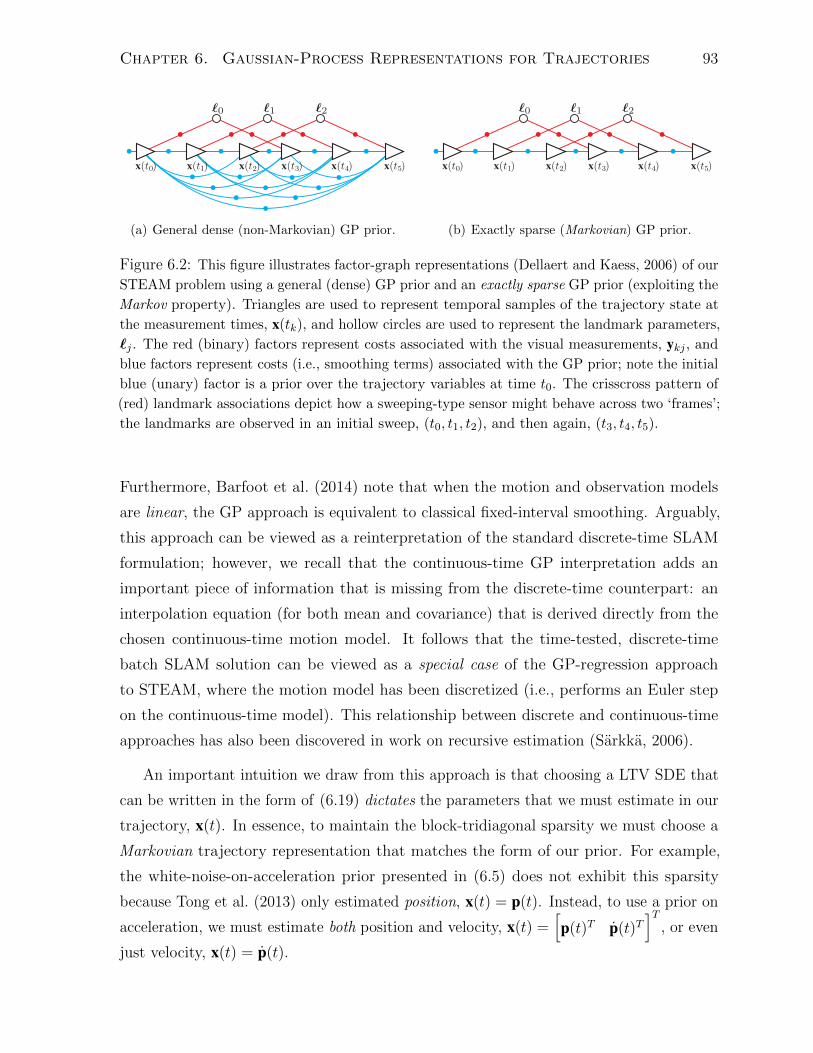
Chapter 6. Gaussian-Process Representations for Trajectories 93
t1x( ) t2x( ) t3x( ) t4x( ) t5x( )
0 2
t0x( )
1
(a) General dense (non-Markovian) GP prior.
0 21
t1x( ) t2x( ) t3x( ) t4x( ) t5x( )t0x( )
(b) Exactly sparse (Markovian) GP prior.
Figure 6.2: This figure illustrates factor-graph representations (Dellaert and Kaess, 2006) of our
STEAM problem using a general (dense) GP prior and an exactly sparse GP prior (exploiting the
Markov property). Triangles are used to represent temporal samples of the trajectory state at
the measurement times, x(tk), and hollow circles are used to represent the landmark parameters,
`j . The red (binary) factors represent costs associated with the visual measurements, ykj , and
blue factors represent costs (i.e., smoothing terms) associated with the GP prior; note the initial
blue (unary) factor is a prior over the trajectory variables at time t0. The crisscross pattern of
(red) landmark associations depict how a sweeping-type sensor might behave across two ‘frames’;
the landmarks are observed in an initial sweep, (t0, t1, t2), and then again, (t3, t4, t5).
Furthermore, Barfoot et al. (2014) note that when the motion and observation models
are linear, the GP approach is equivalent to classical fixed-interval smoothing. Arguably,
this approach can be viewed as a reinterpretation of the standard discrete-time SLAM
formulation; however, we recall that the continuous-time GP interpretation adds an
important piece of information that is missing from the discrete-time counterpart: an
interpolation equation (for both mean and covariance) that is derived directly from the
chosen continuous-time motion model. It follows that the time-tested, discrete-time
batch SLAM solution can be viewed as a special case of the GP-regression approach
to STEAM, where the motion model has been discretized (i.e., performs an Euler step
on the continuous-time model). This relationship between discrete and continuous-time
approaches has also been discovered in work on recursive estimation (Sarkka, 2006).
An important intuition we draw from this approach is that choosing a LTV SDE that
can be written in the form of (6.19) dictates the parameters that we must estimate in our
trajectory, x(t). In essence, to maintain the block-tridiagonal sparsity we must choose a
Markovian trajectory representation that matches the form of our prior. For example,
the white-noise-on-acceleration prior presented in (6.5) does not exhibit this sparsity
because Tong et al. (2013) only estimated position, x(t) = p(t). Instead, to use a prior on
acceleration, we must estimate both position and velocity, x(t) =[p(t)T p(t)T
]T, or even
just velocity, x(t) = p(t).
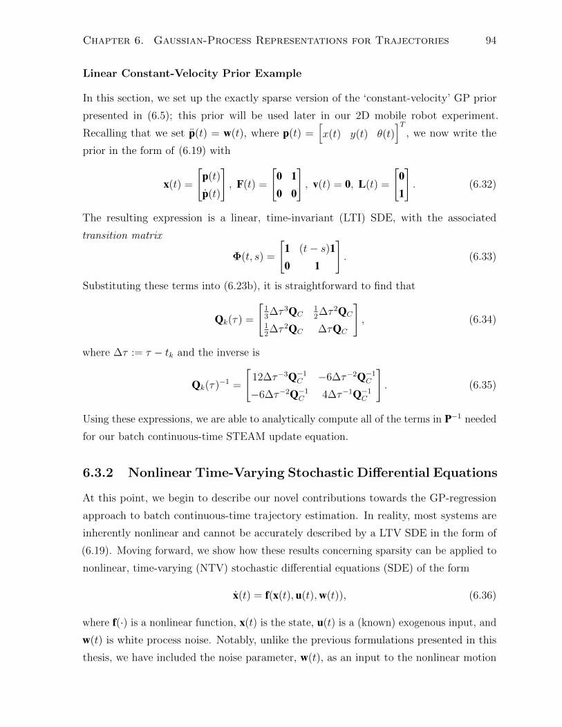
Chapter 6. Gaussian-Process Representations for Trajectories 94
Linear Constant-Velocity Prior Example
In this section, we set up the exactly sparse version of the ‘constant-velocity’ GP prior
presented in (6.5); this prior will be used later in our 2D mobile robot experiment.
Recalling that we set p(t) = w(t), where p(t) =[x(t) y(t) θ(t)
]T, we now write the
prior in the form of (6.19) with
x(t) =
[p(t)
p(t)
], F(t) =
[0 10 0
], v(t) = 0, L(t) =
[01
]. (6.32)
The resulting expression is a linear, time-invariant (LTI) SDE, with the associated
transition matrix
Φ(t, s) =
[1 (t− s)10 1
]. (6.33)
Substituting these terms into (6.23b), it is straightforward to find that
Qk(τ) =
[13∆τ 3QC
12∆τ 2QC
12∆τ 2QC ∆τQC
], (6.34)
where ∆τ := τ − tk and the inverse is
Qk(τ)−1 =
[12∆τ−3Q−1
C −6∆τ−2Q−1C
−6∆τ−2Q−1C 4∆τ−1Q−1
C
]. (6.35)
Using these expressions, we are able to analytically compute all of the terms in P−1 needed
for our batch continuous-time STEAM update equation.
6.3.2 Nonlinear Time-Varying Stochastic Differential Equations
At this point, we begin to describe our novel contributions towards the GP-regression
approach to batch continuous-time trajectory estimation. In reality, most systems are
inherently nonlinear and cannot be accurately described by a LTV SDE in the form of
(6.19). Moving forward, we show how these results concerning sparsity can be applied to
nonlinear, time-varying (NTV) stochastic differential equations (SDE) of the form
x(t) = f(x(t),u(t),w(t)), (6.36)
where f(·) is a nonlinear function, x(t) is the state, u(t) is a (known) exogenous input, and
w(t) is white process noise. Notably, unlike the previous formulations presented in this
thesis, we have included the noise parameter, w(t), as an input to the nonlinear motion

Chapter 6. Gaussian-Process Representations for Trajectories 95
model – this allows for greater freedom in describing how process noise is injected into
x(t). To perform GP regression with a nonlinear process model, we begin by linearizing
the SDE about a continuous-time operating point x(t),
x(t) = f(x(t),u(t),w(t)) ≈ f(x(t),u(t), 0) + F(t)(x(t)− x(t)) + L(t)w(t), (6.37)
where
F(t) =∂f∂x
∣∣∣∣x(t),u(t),0
, L(t) =∂f∂w
∣∣∣∣x(t),u(t),0
. (6.38)
Setting
v(t) = f(x(t),u(t), 0)− F(t)x(t) (6.39)
lets us rewrite (6.37) in the familiar LTV SDE form,
x(t) ≈ F(t)x(t) + v(t) + L(t)w(t), (6.40)
where F(t), v(t), and L(t) are known functions of time, since x(t) is known. Setting the
operating point, x(t), to our best guess of the underlying trajectory at each iteration of
GP regression, we note a similarity in nature to the discrete-time, recursive method of Bell
(1994); in essence, our approach offers a continuous-discrete version of the Gauss-Newton
estimator, using the Gaussian-process-regressor type of approximate bridging between
the measurement times.
Mean and Covariance Functions
Although the equations for calculating the mean, x, and covariance, P, remain the same
as in (6.21) and (6.22), there are a few algorithmic differences and issues that arise due
to the new dependence on the continuous-time operating point, x(t). One difference (in
contrast to using a LTV SDE), is that we must now recalculate x and P at each iteration
of the optimization (since the linearization point is updated). The main algorithmic issue
that presents itself is that the calculation of x and P require integrations involving F(t),
v(t), and L(t), which in turn require the evaluation of x(t) over the time period t ∈ [t0, tK ].
Since an estimate of the posterior mean, x, is stored only at times of interest, we must
make use of the efficient (for our particular choice of process model) GP interpolation
equation derived in Section 6.3.1,
x(τ) = x(τ) + P(τ)P−1(x− x). (6.41)

Chapter 6. Gaussian-Process Representations for Trajectories 96
The problem is that the above interpolation depends (once again) on x and P, which
are the prior variables for which we want to solve. To rectify this circular dependence,
we take advantage of the iterative nature of GP regression and choose to evaluate (6.41)
using the values of x(τ), x, and P(τ)P−1 from the previous iteration.
Another issue with nonlinear process models is that identifying an analytical expression
for the state transition matrix, Φ(t, s) (which is dependent on the form of F(t)), can be
very challenging. Fortunately, the transition matrix can also be calculated numerically
via the integration of the normalized fundamental matrix, Υ(t), where
Υ(t) = F(t)Υ(t), Υ(0) = 1. (6.42)
Storing Υ(t) at times of interest, the transition matrix can then be computed using
Φ(t, s) = Υ(t)Υ(s)−1. (6.43)
In contrast to the LTV SDE system, using a nonlinear process model causes additional
computational costs (primarily due to numerical integrations), but complexity remains
linear in the length of the trajectory (at each iteration), and therefore continues to be
computationally tractable.
Querying the Trajectory
In this section, we discuss the algorithmic details of the GP interpolation procedure as
it pertains to a NTV SDE process model. Recall the standard linear GP interpolation
formulas presented in (6.17), for a single query time, tk ≤ τ < tk+1:
x(τ) = x(τ) + P(τ)P−1(x− x),
P(τ, τ) = P(τ, τ) + P(τ)P−1(
P− P)
P−T P(τ)T .
The final iteration of GP regression (where x = x), provides values for x, P, x, and P;
however, obtaining values for x(τ), P(τ)P−1 (recall the sparse structure in (6.29)), and
P(τ, τ) is not trivial. The suggestion made previously was to use values from the previous
(or in this case, final) iteration. Thus far, the method of storing these continuous-time
functions has been left ambiguous.
The naive way to store x(τ), P(τ)P−1, and P(τ, τ) is to keep the values at all numerical
integration timesteps; the memory requirement of this is proportional to the length of
the trajectory. During the optimization procedure this naive method may in fact be

Chapter 6. Gaussian-Process Representations for Trajectories 97
preferable as it reduces computation time in lieu of additional storage (which is fairly
cheap using current technology). However, for long-term storage, a method that uses a
smaller memory footprint (at the cost of additional computation) may be desirable. The
remainder of this section will focus on identifying the minimal storage requirements, such
that queries remain O(1) complexity.
We begin by examining the mean function; substituting (6.24a) and (6.39), into the
GP interpolation formula above, we have
x(τ) = Φ(τ, tk)xk +
∫ τ
tk
Φ(τ, s)(f(x(s),u(s), 0)− F(s)x(s)
)ds+ P(τ)P−1(x− x). (6.45)
It is straightforward to see how x(τ) can be simultaneously numerically integrated with the
normalized fundamental matrix from (6.42), provided we can evaluate the term P(τ)P−1.
Although we chose to examine the mean function, a similar conclusion can be drawn by
examining the covariance function in (6.24b). Recalling the sparse structure of P(τ)P−1
for an LTV SDE process model, where
Λ(τ) = Φ(τ, tk)−Ω(τ)Φ(tk+1, tk), Ω(τ) = Qk(τ)Φ(tk+1, τ)TQk(tk+1)−1,
we are able to draw two conclusions. First, in the case that an analytical expression
for Φ(t, s) is unavailable, we must store Υ(tk) at the times of interest tk, k = 1 . . . K,
since any numerical integration will involve ‘future’ values of Υ(t) (via the evaluation of
Φ(tk+1, tk), Φ(tk+1, τ), and Qk(tk+1)−1). Second, in the case that L(t) is a time-varying
matrix, we must store Qk(tk+1)−1, k = 0 . . . K − 1, since the evaluation of Qk(tk+1)
−1
requires L(s) (evaluated at x(s)) over the time period [tk−1, tk]. The memory requirements
of this alternative are still proportional to the length of the trajectory, but are greatly
reduced in contrast to the naive method; the added cost is that any new query requires
numerical integration from the nearest time tk to the query time τ (which is order O(1)).
Nonlinear Constant-Velocity Prior Example
Since the main source of acceleration (and probably disturbance) in a standard 2D ground-
robot model is body-centric (i.e., the actuated wheels), we extend the linear GP prior
example from Section 6.3.1 by investigating the use of an alternate ‘constant-velocity’
prior, with white noise affecting acceleration in the robot body frame, ν(t) = w(t). This
nonlinear prior can be written as,
x(t) = f(x(t),u(t),w(t)) =
[0 RIB(θ(t))
0 0
]x(t) + u(t) +
[01
]w(t), (6.46)

Chapter 6. Gaussian-Process Representations for Trajectories 98
where we recall that θ(t) is a component of x(t), and
RIB(θ(t)) =
cos θ(t) − sin θ(t) 0
sin θ(t) cos θ(t) 0
0 0 1
(6.47)
is a rotation matrix between the inertial and robot body frame. The associated Markovian
state is then x(t) =[p(t)T ν(t)T
]T, where ν(t) =
[v(t) u(t) ω(t)
]T= RIB(θ(t))T p(t)
is the robot-oriented velocity (with longitudinal, lateral, and rotational components).
Linearizing about an arbitrary operating point, x(t), the components F(t), v(t) and L(t)
from (6.40) are straightforward to derive. Similar to the linear prior example, described in
Section 6.3.1, we define the exogenous input u(t) = 0; however, recalling (6.39), we note
that v(t) 6= 0. Since expressions for Φ(t, s), and by extension Qk(tk+1), are not obvious,
we will rely on numerical integration for their evaluation.
6.3.3 Training the Hyperparameters
As with any GP regression, we have hyperparameters associated with our mean and
covariance functions. In this problem, the pertinent hyperparameters are x0, P0 and QC .
While we will typically have some information about the initial state (and uncertainty) of
the robot, the matrix QC can be difficult to determine and affects both the smoothness and
length-scale of the class of functions we are considering as motion priors. The standard
approach to selecting this parameter is to use a training dataset (with ground-truth), and
perform optimization using the log marginal likelihood (log-evidence) or its approximation
as the objective function (Rasmussen and Williams, 2006). We begin with the marginal
likelihood equation,
log p(y|QC) = −1
2(y− x)TP−1
σ (y− x)− 1
2log |Pσ| −
n
2log 2π, (6.48a)
Pσ = P(QC) + σ2w1, (6.48b)
where y is a stacked vector of state observations (ground-truth measurements) with
additive noise N (0, σ2w1), x is a stacked vector of the mean equation evaluated at the
observation times, tw, w = 1 . . .W , and P is the covariance matrix associated with x and
generated using the hyperparameters QC . Taking partial derivatives of the marginal
likelihood with respect to the hyperparameters, we get
∂
∂QCij
log p(y|QC) =1
2(y− x)TP−1
σ
∂Pσ∂QCij
P−1σ (y− x)− 1
2tr
(P−1σ
∂Pσ∂QCij
), (6.49)

Chapter 6. Gaussian-Process Representations for Trajectories 99
where we have used ∂P−1σ
∂QCij= −P−1
σ∂Pσ∂QCij
P−1σ .
The typical complexity of hyperparameter training is bottlenecked at O(W 3) due to
the inversion of Pσ (which is typically dense). Given P−1σ , the complexity is then typically
bottlenecked at O(W 2) due to the calculation of ∂Pσ∂QCij
. Fortunately, in the present case,
the computation of the log marginal likelihood can also be done efficiently due to the
sparseness of the inverse kernel matrix, P−1. Despite the addition of observation noise,
σ2w1, causing P−1
σ to be a dense matrix, we are still able to take advantage of our sparsity
by applying the Sherman-Morrison-Woodbury identity to find that
P−1σ = P−1 − P−1
(P−1 +
1
σ2w
1)−1
P−1 = F−TQ−1σ F−1, (6.50)
where we define
Q−1σ :=
(Q−1 −Q−1F−1
(P−1 +
1
σ2w
1)−1
F−TQ−1
). (6.51)
Although explicitly computing P−1σ is of order O(W 2), we note that the product with a
vector, P−1σ v, can be computed in O(W ) time; this is easily observable given that Q−1
is block-diagonal, F−1 is lower block-bidiagonal, and the product (P−1 + 1σ2w
1)−1v can
be computed in O(W ) time using Cholesky decomposition (since P−1 + 1σ2w
1 is block-
tridiagonal). While the two terms in (6.49) can be combined into a single trace function,
it is simpler to study their computational complexity separately. Starting with the first
term, we have
1
2(y− x)TP−1
σ
∂Pσ∂QCij
P−1σ (y− x) =
1
2(y− x)TF−TQ−1
σ
∂Q∂QCij
Q−1σ F−1(y− x), (6.52)
where
∂Q∂QCij
= diag
(0,
∂Q1
∂QCij
, . . . ,∂QK
∂QCij
), (6.53)
and
∂Qj
∂QCij
:=
∫ tj
tj−1
Φ(tj, s)L(s)∂QC
∂QCij
L(s)TΦ(tj, s)T ds,
∂QC
∂QCij
= 1i,j, (6.54)
where 1i,j is a projection matrix with a 1 at the ith row and jth column. Taking advantage
of the sparse matrices and previously mentioned fast matrix-vector products, it is clear
that (6.52) can be computed in O(W ) time (in contrast to the typical O(W 3) time).

Chapter 6. Gaussian-Process Representations for Trajectories 100
Examining the second term, we have
1
2tr
(P−1σ
∂Pσ∂QCij
)=
1
2tr
((F−TQ−1
σ F−1)(
F∂Q∂QCij
FT))
=1
2tr
(∂Q∂QCij
Q−1σ
), (6.55)
which can only be computed in O(W 2), due to the form of Q−1σ . In general, the total
complexity of training for this sparse class of prior is then bottlenecked at O(W 2). A
complexity of O(W ) can only be achieved by ignoring the additive measurement noise,
σ2w1; revisiting the second term of (6.49), and setting Pσ = P, we find that
1
2tr
(P−1 ∂P
∂QCij
)=
1
2tr
(∂Q∂QCij
Q−1
), (6.56)
which can be computed in time O(W ). The effect of ignoring the measurement noise,
σ2w1, is that the trained hyperparameters will result in an underconfident prior; the degree
of this underconfidence depends on the magnitude of the noise we are choosing to ignore.
If accurate ground-truth measurements are available and the size of the training dataset
is very large, this approximation may be beneficial.
6.3.4 Mobile Robot Experiment
To validate our nonlinear extension against the linear method of Barfoot et al. (2014)
and the dense method of Tong et al. (2013), we utilize the same 2D mobile robot dataset
(depicted in Figure 6.3). The experiment used a P3-AT mobile robot, equipped with a
Hokuyo URG-04LX-UG01 laser rangefinder, driving through a ‘forest’ of 17 plastic-tube
landmarks. The dataset includes odometry measurements, range/bearing measurements
(to the plastic-tubes), and ground-truth for both the robot trajectory and landmark
positions (provided by a Vicon motion capture system).
Figure 6.3: Photograph of the experi-
ment conducted by Tong et al. (2013).
Four estimators are implemented for comparison:
(i) the algorithm described by Tong et al. (2013),
GP-Pose-Dense, which has a dense inverse kernel
matrix, (ii) a naive version of Markovian STEAM
estimator, GP-Traj-Dense, which is based on the LTI
SDE prior example described in Section 6.3.1, but
does not exploit sparsity, (iii) a sparsity-exploiting
version of the STEAM estimator, GP-Traj-Sparse-
LTI, which uses the same LTI SDE prior, and (iv)
a sparsity-exploiting STEAM estimator, GP-Traj-Sparse-NTV, that uses the NTV SDE

Chapter 6. Gaussian-Process Representations for Trajectories 101
Table 6.1: This table contains results from the k-folds hyperparameter training for both the
LTI and NTV priors described in Sections 6.3.1 and 6.3.2. Specifically, it contains the mean and
standard deviation of the three hyperparameters (diagonal of QC) and average training time for
a set of hyperparameters
QC,11 [µ± σ] QC,22 [µ± σ] QC,33 [µ± σ] Average Time [s]
LTI 1.679e-2 ± 9.077e-4 7.841e-3 ± 6.863e-4 5.930e-2 ± 1.817e-3 22.56
NTV 2.811e-2 ± 6.022e-4 2.244e-4 ± 1.923e-5 5.993e-2 ± 1.710e-3 65.16
prior example described in Sections 6.3.2. Note that we do not implement nonlinear
versions of the first two estimators, GP-Pose-Dense and GP-Traj-Dense, because they
are only of interest with regard to computational performance.
Measurement Models
We have access to two types of measurements: range/bearing to landmarks (using a laser
rangefinder) and wheel odometry (in the form of robot-oriented velocity). For both state
parameterizations, the range/bearing measurement model takes the form
ykj = grb(x(tk), `j) + nkj =
[√(`j,1 − x(tk))2 + (`j,2 − y(tk))2
atan2(`j,2 − y(tk), `j,1 − x(tk))
]+ nkj. (6.57)
The wheel odometry measurement model gives the longitudinal and rotational speeds of
the robot, taking the form
yk = gwo(x(tk)) + nk =
[cos θ(tk) sin θ(tk) 0
0 0 1
]p(tk) + nk (6.58)
for the LTI SDE prior, and
yk = gwo(x(tk)) + nk =
[1 0 0
0 0 1
]ν(tk) + nk (6.59)
for the NTV SDE prior. Note that in both cases the velocity information is extracted
easily from the state since we are estimating it directly.
Hyperparameters
For this experiment, we obtained QC for both the LTI and NTV priors by constraining it
to be a diagonal matrix and taking the data-driven training approach using log marginal
likelihood (with ground-truth measurements) described in Section 6.3.3. Specifically, five

Chapter 6. Gaussian-Process Representations for Trajectories 102
Table 6.2: This table contains estimation error results from both the k-folds cross-validation
and roughly 15-minute test set for both the LTI and NTV priors.
Average K-fold Validation Error Test Set Error
Trans.
Err. [m]
Angular
Err. [deg]
Landmark
Err. [m]
Trans.
Err. [m]
Angular
Err. [deg]
Landmark
Err. [m]
LTI 7.493e-2 3.282 0.100 7.419e-2 2.274 8.246e-2
NTV 8.002e-2 3.626 0.111 7.301e-2 2.284 9.059e-2
minutes of the roughly 20-minute dataset were set aside for training; the five minutes of
training data are then split into ten 30-second trajectories (each having 300 ground-truth
measurements) that are used for k-folds training and cross-validation. The remaining 15
minutes of data are used as a test set to perform a final evaluation of the estimator.
Results from the training, validation, and testing can be found in Tables 6.1 and 6.2.
Notably, each of the ten folds of hyperparameter training produced a very similar set of
values for our model of QC . Since the performance metric we are most interested in is the
accuracy of the estimator, the k-fold cross-validations and final test were performed by
solving the proposed GP regression problem with the given sets of hyperparameters and
then comparing the trajectory estimates to ground-truth. The average validation errors
over the ten folds are fairly good for both the LTI and NTV priors, but more importantly
were very representative of the errors on the final test set. An interesting advantage of
the NTV prior is that it is rotationally invariant; note that the values of QC,11 and QC,22
for the LTI prior (related to x and y motions, respectively) are distinctly different (a
product of the training data).
Given that our hyperparameters have a physical interpretation (in this case, related
to our prior knowledge of vehicle accelerations), we note that the goal of training should
be to find a QC that generalizes well for a specific platform (it cannot be assumed that a
single choice of QC will generalize well for different types of vehicles). With regard to the
sensitivity of the hyperparameters, it is our experience that when relatively high-frequency
measurements are available, the estimator is not overly sensitive to a more inclusive
(slightly underconfident) prior; rather, it is more ‘dangerous’ to choose a restrictive
(overconfident) prior that may preclude the true underlying motion.
Computational Cost
In order to quantify the computational gain associated with using an exactly-sparse GP
prior, we time the four batch estimators for varying lengths of the dataset (notably,

Chapter 6. Gaussian-Process Representations for Trajectories 103
(a) Kernel matrix construction time. (b) Optimization time per iteration.
(c) Interpolation time per additional query time. (d) Total computation time.
Figure 6.4: This figure presents the computational costs associated with the four batch STEAM
estimators. Notably, the sparse algorithms exhibit either constant or linear cost (in trajectory
length) for all of the timed components (including the full solution). The estimators were timed
in Matlab with a 2.4GHz i7 processor and 8GB of 1333MHz DDR3 RAM. Note the change from
a linear to a log scale in the upper part of each plot.
we use the full 20 minutes of data for timing purposes). The timing results, presented
in Figure 6.4, are broken down into several pieces. Note that the GP-Pose-Dense and
GP-Traj-Dense estimators are significantly slower in all aspects since they use/assume a
dense kernel matrix. For the exactly sparse estimators, GP-Traj-Sparse-LTI and GP-Traj-
Sparse-NTV, we verify that the interpolation time is constant for a single query, and that
the kernel construction time, iteration time, and total time are all linear in the number of
measurements; these approaches significantly outperform the other algorithms.
The additional cost of the GP-Traj-Sparse-NTV algorithm over the GP-Traj-Sparse-
LTI algorithm in kernel construction time is due to the linearization and numerical
integration of the prior mean and covariance. The optimization time of the GP-Traj-
Sparse-NTV algorithm is also affected because the kernel matrix must be reconstructed
from a new linearization of the prior during every optimization iteration. Finally, the GP-
Traj-Sparse-NTV algorithm also incurs some numerical integration cost in interpolation
time, but it is constant and very small.
Increasing Nonlinearity
In a problem with fairly accurate and high-rate measurements, we note that both the
GP-Traj-Sparse-LTI and GP-Traj-Sparse-NTV estimators provide similar accuracy; a

Chapter 6. Gaussian-Process Representations for Trajectories 104
(a) GP-Traj-Sparse-LTI trajectory sample. (b) GP-Traj-Sparse-NTV trajectory sample.
Figure 6.5: The smooth trajectories and 3σ covariance envelope estimates produced by the
GP-Traj-Sparse estimators (both linear and nonlinear) over a short segment of the dataset.
qualitative result is depicted in Figure 6.5, where both the posterior mean and covariance
of the continuous-time trajectory are queried and plotted at a rate of 10 Hz. Notably, the
GP-Traj-Sparse-NTV algorithm differed slightly from the others (the dense estimator result
is not shown, but was remarkably similar to that of the sparse linear prior); qualitatively,
we found that the trajectory estimated by the GP-Traj-Sparse-NTV algorithm more
accurately matched the local shape of the ground-truth on many occasions (note the
insets in Figure 6.5). Also, it is clear from the plotted 3σ covariance envelope that the
estimate from the GP-Traj-Sparse-NTV algorithm tends to be more uncertain.
In order to expose the benefit of a nonlinear prior based on the expected motion of the
vehicle, we increase the nonlinearity of the problem by reducing measurement frequency.
The result of varying range measurement frequency, with and without the use of odometry
measurements, is shown in Figure 6.6. In general, it is clear that as the interval between
range measurements is increased, the GP-Traj-Sparse-NTV estimator is able to produce a
more accurate estimate of the continuous-time pose (translation and rotation) than the
GP-Traj-Sparse-LTI estimator. In the case that the 1 Hz odometry measurements are
available, as seen in Figure 6.6(a), the difference in the rotation estimates is small, because
the GP-Traj-Sparse-LTI estimator has a reasonable amount of information about its
heading; however, in the case that the odometry measurements are unavailable, as seen in
Figure 6.6(b), the advantage of the nonlinear prior, provided by the GP-Traj-Sparse-NTV
estimator, becomes more prominent.
In order to gain some qualitative intuition about how the continuous-time estimates
are affected by the reduction of measurement frequency, Figure 6.7 shows the trajectories
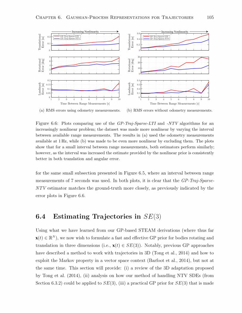
Chapter 6. Gaussian-Process Representations for Trajectories 105
Increasing Nonlinearity
(a) RMS errors using odometry measurements.
Increasing Nonlinearity
(b) RMS errors without odometry measurements.
Figure 6.6: Plots comparing use of the GP-Traj-Sparse-LTI and -NTV algorithms for an
increasingly nonlinear problem; the dataset was made more nonlinear by varying the interval
between available range measurements. The results in (a) used the odometry measurements
available at 1 Hz, while (b) was made to be even more nonlinear by excluding them. The plots
show that for a small interval between range measurements, both estimators perform similarly;
however, as the interval was increased the estimate provided by the nonlinear prior is consistently
better in both translation and angular error.
for the same small subsection presented in Figure 6.5, where an interval between range
measurements of 7 seconds was used. In both plots, it is clear that the GP-Traj-Sparse-
NTV estimator matches the ground-truth more closely, as previously indicated by the
error plots in Figure 6.6.
6.4 Estimating Trajectories in SE(3)
Using what we have learned from our GP-based STEAM derivations (where thus far
x(t) ∈ RN ), we now wish to formulate a fast and effective GP prior for bodies rotating and
translation in three dimensions (i.e., x(t) ∈ SE(3)). Notably, previous GP approaches
have described a method to work with trajectories in 3D (Tong et al., 2014) and how to
exploit the Markov property in a vector space context (Barfoot et al., 2014), but not at
the same time. This section will provide: (i) a review of the 3D adaptation proposed
by Tong et al. (2014), (ii) analysis on how our method of handling NTV SDEs (from
Section 6.3.2) could be applied to SE(3), (iii) a practical GP prior for SE(3) that is made

Chapter 6. Gaussian-Process Representations for Trajectories 106
(a) With odometry measurements. (b) Without odometry measurements.
Figure 6.7: Plots showing the GP-Traj-Sparse-LTI and -NTV estimates for the same small
trajectory subsection as Figure 6.5, with an interval between range measurements of 7 seconds.
Results in (a) used odometry measurements, while (b) did not.
efficient by approximating nonlinear kinematics in a piecewise fashion, (iv) a description
of methods that allow us to process high-rate data and loop-closures in real time, and
(v) experimental validation using the appearance-based lidar dataset.
6.4.1 Background – Adapting for SE(3)
We begin by discussing the GP prior formulation and assumptions used by Tong et al.
(2014) to formulate a 3D adaptation of their GPGN algorithm. Recalling the problem
formulation described in Section 6.2.1, we now shift the GP regression problem to consider
state variables that belong to the matrix Lie group SE(3). In continuous-time, Tong et al.
(2014) define the trajectory state as
x(t) := T(t) = Tt,i, F−→t := F−→rob(t), (6.60)
where F−→rob(t) is the time-varying robot frame and T(t) is the transformation that
describes the robot pose (at time t) with respect to an inertial frame, F−→i. Following our
standard approach to GP-based STEAM, we discretize the trajectory at the measurement
times; notably, this process mirrors the standard, three-dimensional, discrete-time SLAM
formulation, discussed in Section 3.2.3, where we have the discrete state collection,
x = T0,i,T1,i, . . . ,Tk,i, . . . ,TK,i, F−→k := F−→rob(tk), (6.61)
and the associated perturbation vector
δx :=[δξT0,i . . . δξ
Tk,i . . . δξ
TK,i
]T, (6.62)
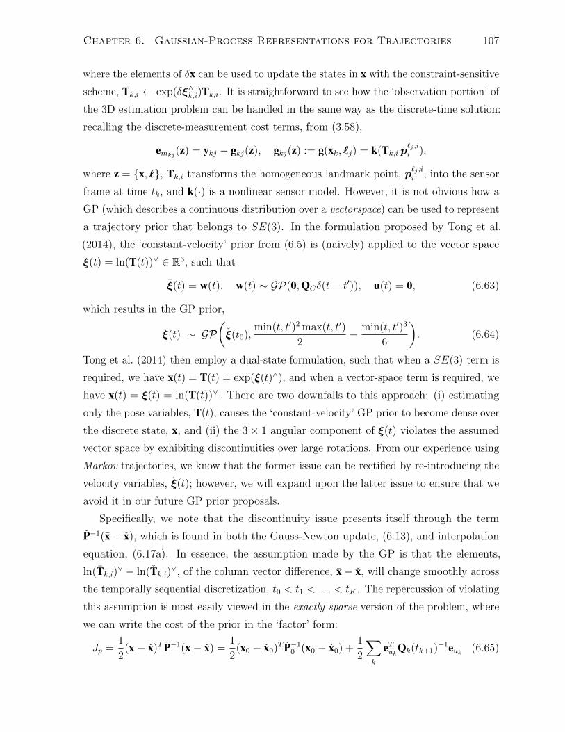
Chapter 6. Gaussian-Process Representations for Trajectories 107
where the elements of δx can be used to update the states in x with the constraint-sensitive
scheme, Tk,i ← exp(δξ∧k,i)Tk,i. It is straightforward to see how the ‘observation portion’ of
the 3D estimation problem can be handled in the same way as the discrete-time solution:
recalling the discrete-measurement cost terms, from (3.58),
emkj(z) = ykj − gkj(z), gkj(z) := g(xk, `j) = k(Tk,i p`j ,ii ),
where z = x, `, Tk,i transforms the homogeneous landmark point, p`j ,ii , into the sensor
frame at time tk, and k(·) is a nonlinear sensor model. However, it is not obvious how a
GP (which describes a continuous distribution over a vectorspace) can be used to represent
a trajectory prior that belongs to SE(3). In the formulation proposed by Tong et al.
(2014), the ‘constant-velocity’ prior from (6.5) is (naively) applied to the vector space
ξ(t) = ln(T(t))∨ ∈ R6, such that
ξ(t) = w(t), w(t) ∼ GP(0,QCδ(t− t′)), u(t) = 0, (6.63)
which results in the GP prior,
ξ(t) ∼ GP(ξ(t0),
min(t, t′)2 max(t, t′)
2− min(t, t′)3
6
). (6.64)
Tong et al. (2014) then employ a dual-state formulation, such that when a SE(3) term is
required, we have x(t) = T(t) = exp(ξ(t)∧), and when a vector-space term is required, we
have x(t) = ξ(t) = ln(T(t))∨. There are two downfalls to this approach: (i) estimating
only the pose variables, T(t), causes the ‘constant-velocity’ GP prior to become dense over
the discrete state, x, and (ii) the 3× 1 angular component of ξ(t) violates the assumed
vector space by exhibiting discontinuities over large rotations. From our experience using
Markov trajectories, we know that the former issue can be rectified by re-introducing the
velocity variables, ξ(t); however, we will expand upon the latter issue to ensure that we
avoid it in our future GP prior proposals.
Specifically, we note that the discontinuity issue presents itself through the term
P−1(x− x), which is found in both the Gauss-Newton update, (6.13), and interpolation
equation, (6.17a). In essence, the assumption made by the GP is that the elements,
ln(Tk,i)∨ − ln(Tk,i)
∨, of the column vector difference, x− x, will change smoothly across
the temporally sequential discretization, t0 < t1 < . . . < tK . The repercussion of violating
this assumption is most easily viewed in the exactly sparse version of the problem, where
we can write the cost of the prior in the ‘factor’ form:
Jp =1
2(x− x)T P−1(x− x) =
1
2(x0 − x0)T P−1
0 (x0 − x0) +1
2
∑k
eTukQk(tk+1)−1euk (6.65)

Chapter 6. Gaussian-Process Representations for Trajectories 108
where the errors terms, euk , are exactly (Barfoot et al., 2014)
euk = (xk+1 − xk+1)−Φ(tk+1, tk)(xk − xk). (6.66)
Notably, use of the ln(·)∨ operator will cause a large discontinuity to occur between xk and
xk+1 when the two rotation parameters straddle the −π/π radian threshold; the GP prior
will view this discontinuity as a large angular ‘error’ and will inflict a strong penalization
that is not warranted. In effect, priors that exhibit this issue are only useful for short
or specific trajectories that do not exhibit large rotations. Finally, we note that Tong
et al. (2014) make the (ad hoc) assumption that vector space differences, ln(T)∨− ln(T)∨,
can be replaced with the operation ln(TT−1)∨; although their proposed prior mean is not
time-varying (i.e., T(t) = T(t0)), it is noted that this assumption would help to avoid
discontinuities if the prior quantities, Tk,i, closely modelled the estimates Tk,i.
6.4.2 Nonlinear GP Regression for SE(3)
Moving forward, we now wish to exploit the exactly sparse GP priors described in
Section 6.3 for trajectories that belong to SE(3). Recalling the nonlinear kinematics
discussed in Chapter 5, we are motivated to use the nonlinear SDE
T(t) = $(t)∧T(t), (6.67a)
$(t) = w′(t), w′(t) ∼ GP(0,Q′Cδ(t− t′)), (6.67b)
where$(t) =[ν(t)ω(t)
]∈ R6 is the body-centric velocity (with linear and angular components,
ν(t) and ω(t)), and the zero-mean, white-noise Gaussian process, w′(t), is injected directly
onto the body-centric acceleration, $(t). It follows that the Markovian trajectory state
we wish to estimate is
x(t) = T(t),$(t) ∈ SE(3)× R6. (6.68)
Recalling the (novel) GP linearization methodology, presented in Section 6.3.2, we
now show how it can be extended to SE(3) by using the familiar constraint-sensitive
perturbations
T(t) = exp(δξ(t)∧)T(t), $(t) = $(t) + δ$(t). (6.69)

Chapter 6. Gaussian-Process Representations for Trajectories 109
Recalling the perturbed kinematics derived in Chapter 5, (5.23), we apply a similar
methodology to the SDE in (6.67) to find the nominal and perturbed components:
˙T(t) = $(t)∧T(t), (6.70a)[δξ(t)
δ$(t)
]︸ ︷︷ ︸
δx(t)
≈[$(t)f 1
0 0
]︸ ︷︷ ︸
F(t)
[δξ(t)
δ$(t)
]︸ ︷︷ ︸
δx(t)
+
[0
− ˙$(t)
]︸ ︷︷ ︸
v(t)
+
[01
]︸︷︷︸L(t)
w′(t). (6.70b)
Following the standard GP approach, we discretize the trajectory state, x(t), at the
measurement times, tk, to form the discrete state collection,
x = T0,i,$0, . . . ,Tk,i,$k . . . ,TK,i,$K, F−→k := F−→rob(tk), (6.71)
with the associated perturbation vector
δx :=[δξ(t0)T δ$(t0)T . . . δξ(tk)
T δ$(tk)T . . . δξ(tK)T δ$(tK)T
]T. (6.72)
In order to utilize the nonlinear SDE (which includes non-vectorspace state variables)
in the GP-regression-based localization problem, (6.13), we first note that the vector
difference, x − x, can be replaced with expected value of the perturbation, E[δx]. In
essence, E[δx] can be thought of as the difference between x and x (e.g., over the SE(3)
manifold). This gives us the equivalent Gauss-Newton update equation:
(P−1 + GTR−1G
)δx? = P−1E[δx] + GTR−1(y− g), (6.73)
where we require expressions for the ‘expected’ perturbation, E[δx], and inverse covariance,
P−1. Recalling the methodology from Section 6.3.2 once more, we note that these terms
can be found by numerically integrating the SDE in (6.70b), via (6.21) and (6.22). With
some effort, we also determine that the corresponding transition function for (6.70b) is:
Φ(t, τ) =
[T (t)T (τ)−1 T (t)
∫ tτT (s)−1ds
0 1
], (6.74)
which can be verified by checking the conditions
Φ(t, τ) = F(t)Φ(t, τ), Φ(τ, τ) = 1. (6.75)

Chapter 6. Gaussian-Process Representations for Trajectories 110
The first condition is verified by using the second fundamental theorem of calculus,
Φ(t, τ) =
ddt T (t)T (τ)−1 d
dtT (t)
∫ tτT (s)−1ds
0 0
=
[˙T (t)T (τ)−1 ˙T (t)
∫ tτT (s)−1ds+ T (t)T (t)−1
0 0
]
=
[$(t)fT (t)T (τ)−1 $(t)fT (t)
∫ tτT (s)−1ds+ 1
0 0
]
=
[$(t)f 1
0 0
]Φ(t, τ) = F(t)Φ(t, τ), (6.76)
and the second by simple substitution
Φ(τ, τ) =
[T (τ)T (τ)−1 T (τ)
∫ ττT (s)−1ds
0 1
]=
[1 00 1
]. (6.77)
To evaluate all of the numerical integrals (such as the one in Φ(t, τ)), we recall that
we must maintain a continuous-time operating point, x(t). Furthermore, to construct
the terms Qk(tk+1)−1 (which can be used to build P−1), the substitution of Φ(t, τ) into
(6.23b) results in a double numerical integral of T (t). Alas, while this 3D extension of
the nonlinear technique presented in Section 6.3.2 could be used to formulate an MAP
estimator for the dynamically motivated GP prior in (6.67), the amount of numerical
integration and bookkeeping required in this scheme is off-putting. Instead, since our
goal is to produce a scheme that is both fast and effective, we will investigate the use of a
piecewise approximation that allows us to closely model the nonlinear kinematics in (6.67)
when the motion between measurement times is small, or of nearly ‘constant-velocity’.
6.4.3 A Piecewise, Locally Linear GP Prior for SE(3)
Motivated by our investigation of the global nonlinear kinematics in (6.67), we note that
many of the laborious numerical integrals that arise from linearization can be (greatly)
simplified by assuming that the velocity estimate, $(t), is piecewise-constant (disjoint at
the measurement times). This observation motivates us to more closely inspect the nature
of the nonlinear SDE. Specifically, our aim is to break the global nonlinear SDE into an
equivalent, piecewise sequence of local SDEs (using the Markov property) and then to find
a reasonable approximation that can be used to make the piecewise segments linear.

Chapter 6. Gaussian-Process Representations for Trajectories 111
Temporal Discretization of the Nonlinear Kinematics
The formulation of our approximation begins by deriving an equivalent expression for the
nonlinear kinematics in (6.67), using the Lie algebra space, se(3). Using the identity
d
dtexp(A(t)) =
∫ 1
0
exp(αA(t))dA(t)
dtexp((1− α)A(t))dα, (6.78)
and the exponential map, T(t) = exp(ξ(t)∧), we rearrange (6.67) to find that
$(t) =(
T(t)T(t)−1)∨
=
(∫ 1
0
T(t)αξ(t)∧T(t)−αdα
)∨=
∫ 1
0
T (t)αdα ξ(t). (6.79)
Recalling the definition of J (·), the (left) Jacobian of SE(3), in (3.43), it follows that
ξ(t) = J (ξ(t))−1$(t), (6.80)
which is an equivalent expression for the nonlinear kinematics in (6.67a). Using this new
relationship, the nonlinear SDE in (6.67) can be written as[ξ(t)
$(t)
]=
[0 J (ξ(t))−1
0 0
][ξ(t)
$(t)
]+
[01
]w′(t). (6.81)
Notably, linearizing this new expression for the NTV SDE will result in an equally
overwhelming collection of numerical integrals. However, this new form reveals an
interesting case (i.e., J (ξ(t)) ≈ 1) where the NTV SDE may be closely approximated
by a LTI SDE. Analyzing the relationship in (6.80), we note two conditions for which
ξ(t) ≈ $(t): (i) when ξ(t) is small, we have that J (ξ(t)) ≈ 1, and (ii) when ξ(t) and
$(t) are nearly parallel (i.e., ξ(t)f$(t) ≈ 0) we have that J (ξ(t))−1$(t) ≈$(t); this
second condition is fulfilled when velocity is near constant (i.e., ξ(t) ≈ (t− t0)$(t)).
In general, it is not reasonable to assume that ξ(t) will remain small or parallel to
$(t) over long trajectories. However, we note that the Markov property allows us to
discretize the NTV SDE in a piecewise fashion. In the context of our GP regression
problem, it is logical for us to perform this discretization at the sequence of measurement
times, t0 < t1 < . . . < tK . Injecting a discretization point into T(t), we have that
T(t) =d
dt
(T(t)T(tk)
−1T(tk))
= Tt,tkT(tk), F−→t := F−→rob(t). (6.82)
Equating this to (6.67a) and rearranging, we (unsurprisingly) find that
Tt,tk = $(t)∧T(t)T(tk)−1 = $(t)∧Tt,tk . (6.83)

Chapter 6. Gaussian-Process Representations for Trajectories 112
Defining the local pose variable
ξk(t) := ln(T(t)T(tk)−1)∨, tk ≤ t ≤ tk+1, (6.84)
we also (unsurprisingly) find that
ξk(t) = J (ξk(t))−1$(t). (6.85)
Therefore, by using the local pose variable definition, ξk(t), the NTV SDE in (6.81) can
be broken up into the sequence of local NTV SDEs:[ξk(t)
$(t)
]=
[0 J (ξk(t))
−1
0 0
][ξk(t)
$(t)
]+
[01
]w′(t), tk ≤ t ≤ tk+1. (6.86)
Notably, the concatenation of these local NTV SDEs results in a global NTV SDE that
is equivalent to both (6.67) and (6.81). Recalling our analysis of (6.80), we are now
able to make the (far more) reasonable assumption that ξk(t) ≈$(t) (and by extension
ξk(t) ≈ $(t)) when the local motion, ξk(t), is small or of nearly constant velocity, over
the (short) time interval t ∈ [tk, tk+1]. However, rather than make approximations directly
to (6.86) (i.e., J (ξk(t))−1 ≈ 1), we instead choose to construct an exact sequence of local
LTI SDEs (that approximate the local NTV SDEs):
γk(t)︷ ︸︸ ︷[ξk(t)
ξk(t)
]=
F(t)︷ ︸︸ ︷[0 10 0
] γk(t)︷ ︸︸ ︷[ξk(t)
ξk(t)
]+
L(t)︷︸︸︷[01
]w(t), tk ≤ t ≤ tk+1, (6.87)
where we assert that w′(t) ≈ w(t) ∼ GP(0,QCδ(t− t′)), when velocity is near constant.
Notably, by choosing to use an exact SDE, we will also have exact expressions for both
the GP-prior cost terms and the interpolation equations. It follows from the (familiar)
form of (6.87) that the general solution to our local LTI SDE is
γk(t) = Φ(t, tk)γk(tk) +
∫ t
tk
Φ(t, s)L(t)w(s) ds, tk ≤ t ≤ tk+1, (6.88)
where the state transition function is simply
Φ(t, t′) =
[1 (t− t′)10 1
]. (6.89)
Notably, in the absence of noise (i.e., w′(t) = w(t) = 0), the integral of the global SDE
and concatenated local LTI SDEs will produce equivalent constant-velocity trajectories

Chapter 6. Gaussian-Process Representations for Trajectories 113
local
global
Figure 6.8: This figure depicts the relationships between the local pose variable, ξk(t), and
the global trajectory state, x(t) = T(t),$(t). The proposed piecewise GP prior approximates
the kinematically motivated SDE in (6.67) by defining a sequence of local LTI SDEs, where we
assume that the local variable, ξk(t), is noisy between the measurements times, tk and tk+1.
(using the same initial conditions). Relating this local GP prior definition back to our
(desired) global state representation, (6.68), we note that it is simple to convert from
x(t) = T(t),$(t) to γk(t) = ξk(t), ξk(t) by using the equations in (6.84) and (6.85);
the relationship between ξk(t) and the global state variables is depicted in Figure 6.8.
Exploiting these relationships (through substitution), it becomes straightforward to define
a GP prior from the sequence of local LTI SDEs in (6.87), while estimating the state
representation x(t) = T(t),$(t) – all without approximation. Furthermore, we note
that the mean and covariance associated with x(t) can be propagated continuously across
the measurement times (from one local SDE to the next).
In summary our sequence of local LTI SDEs: (i) accomplish the result of a global
SDE in a piecewise fashion, and (ii) approximate the full nonlinear SDE in (6.67) when
motion between each pair of measurement times, tk and tk+1, is either small or of nearly
constant velocity. This is verified experimentally by comparing the mean and covariance
of our concatenated GP prior to a Monte Carlo simulation of (6.67) (see Figure 6.9).
Analytical Nonlinear Smoothing Factors for SE(3)
In order to linearize our GP prior cost with respect to the global state representation, x(t),
we opt to take a factor-graph view of the STEAM problem (recall Figure 6.2). Notably,
the objective function cost associated with the exactly sparse class of GP priors can be

Chapter 6. Gaussian-Process Representations for Trajectories 114
(a) Low Angular Velocity (b) High Angular Velocity
Figure 6.9: This figure compares the GP prior formed from our concatenated local LTI
SDEs (solid black constant-velocity mean and 3σ ‘banana’ covariances) against a Monte Carlo
simulation of the nonlinear SDE from equation (6.67) (the 2000 blue trajectory samples).
To make the comparison easier to visualize, noise was injected only in the (body-centric) x-
component of translation and z-component of rotation. The banana shapes are 3σ great circles
of the six-degree-of-freedom uncertainty hyperellipsoid, mapped onto the xy-plane.
reformulated as (Barfoot et al., 2014):
Jp(x) =1
2(x− x)T P−1(x− x) =
1
2eTp0
P−10 ep0 +
1
2
∑k
eTukQk(tk+1)−1euk , (6.90)
where eTp0P−1
0 ep0 is a unary factor associated with position and velocity at the initial time,
t0, and the (binary) smoothing terms have the exact form:
euk = γk(tk+1)− γk(tk+1)−Φ(tk+1, tk) (γk(tk)− γk(tk)) , (6.91)
with the (familiar) analytical covariance expression
Qk(τ) =
[13∆τ 3
kQC12∆τ 2
kQC
12∆τ 2
kQC ∆τ kQC
], Qk(τ)−1 =
[12∆τ−3
k Q−1C −6∆τ−2
k Q−1C
−6∆τ−2k Q−1
C 4∆τ−1k Q−1
C
], (6.92)
where ∆τ k := τ − tk. Without exogenous control inputs, the prior mean is simply
γk(t) = E[γk(t)] = Φ(t, tk)γk(tk), (6.93)
and our expression for euk simplifies to
euk = γk(tk+1)−Φ(tk+1, tk)γk(tk). (6.94)

Chapter 6. Gaussian-Process Representations for Trajectories 115
Substituting the expressions from (6.84) and (6.85) into γk(t),
γk(t) =
[ξk(t)
ξk(t)
]=
[ln(T(t)T−1
k,i )∨
J (ln(T(t)T−1k,i )∨)−1$(t)
], (6.95)
it follows that our smoothing terms have the exact nonlinear form:
euk =
[ln(Tk+1,iT−1
k,i )∨ − (tk+1 − tk)$k
J (ln(Tk+1,iT−1k,i )∨)−1$k+1 −$k
], (6.96)
where Tk,i, $k, Tk+1,i, and$k+1 are temporally adjacent elements of the discretized global
state vector, x, defined in (6.71). Inspecting (6.96), it is pleasing that the result is intuitive:
beginning with a prior akin to white-noise-on-acceleration (i.e., ξk(t) = w(t)), the global
state variables are penalized for deviating from a body-centric, constant-velocity trajectory.
In the case that $k = $k+1, and Tk+1,i = exp((tk+1 − tk)$∧k ) Tk,i (which agrees with
the nonlinear kinematics in (6.67)), we have that euk = 0. Furthermore, these local
errors are unaffected by discontinuities (assuming that the rotation between consecutive
measurement times is less than π). At this point, we may wish to make the simplifying
assumption that J (ln(Tk+1,iT−1k,i )∨)−1$k+1 ≈ $k+1; however, for completeness, this
thesis will continue to use the exact form above.
Concerning the initial factor, eTp0P−1
0 ep0 , we note that in the STEAM context we will
typically lock the initial pose (but not the velocity). Defining ep0 := $0 − $0, the total
set of hyperparameters in our approach is: QC , $0, and P0. In practice, when little is
known about the a priori initial velocity, $0, it is often safe to over-inflate the covariance
matrix P0; this allows the initial posterior estimate, $0, to be determined primarily
through the binary smoothing terms.
Efficient GP-Based STEAM for SE(3)
In this section, we demonstrate how our sparse set of nonlinear prior factors can be
incorporated into the STEAM problem. We begin by recalling the optimization problem
we wish to solve
z = argminz
J(z), J(z) = Jm(z) + Jp(x), (6.97)
where z = x, `, J(z) is our objective function, Jm(z) contains the costs associated with
the measurements/observations, and Jp(x) is the cost of our GP prior. The form of our
GP prior cost, Jp(x), was previously shown in (6.90), where the exact nonlinear cost terms,

Chapter 6. Gaussian-Process Representations for Trajectories 116
euk , are defined in (6.91). Since the trajectory state, x(t), has been discretized at the
measurement times, it is straightforward to see that Jm(z) has the familiar form
Jm(z) :=1
2
∑kj
eTmkjR−1kj emkj , (6.98)
where
emkj(z) = ykj − gkj(z), gkj(z) := k(hkj(z)), hkj(z) = Tk,i p`j ,ii , (6.99)
and Rkj is the covariance of the measurement noise.
In order to leverage our standard Gauss-Newton machinery, described in Section 3.1.2,
we linearize our cost terms using the constraint-sensitive perturbations:
Tk,i = exp((δξk,i)∧)Tk,i, $k = $k + δ$k, ˆ
j = ¯j + δ`j. (6.100)
It follows that the standard linearized measurement costs are simply
emkj(z + δz) = ykj − k(Tk,i p`j ,ii )−Gkjδz, (6.101)
Gkj :=[KkjHx,kjPx,k KkjH`,kjP`,j
], (6.102)
where Kkj, Hx,kj, and H`,kj were defined in (3.62) and (3.64), and Px,k and P`,j are
projection matrices that select the kth element of x and the jth of `. The linearization of
the prior costs, in (6.96), require more effort. We begin by deriving the (approximate)
relationships we require; recalling the relationship from Chapter 3, in (3.42):
Tb,a = exp(ξ∧b,a) ≈ exp(δξ∧b,a) exp(ξ∧b,a) ≈ exp
((ξb,a + J (ξb,a)
−1δξb,a)∧), (6.103)
it is straightforward to see that
ln(Tb,a)∨ ≈ ln(Tb,a)
∨ + J −1b,aδξb,a, J b,a := J (ln(Tb,a)
∨), (6.104)
which leads us to the (approximate) linearization
J (ln(Tb,a)∨)−1$ ≈ J
(ln(Tb,a)
∨ + J (ln(Tb,a)∨)−1δξb,a
)−1($ + δ$)
≈ J −1b,a$ −
1
2
(J −1
b,aδξb,a)f$ + J −1
b,aδ$,
= J −1b,a$ +
1
2$fJ −1
b,aδξb,a + J −1b,aδ$. (6.105)
Finally, using the relationship δξb,a ≈ δξb − T b,aδξa, combined with the expressions in
(6.104) and (6.105), our linearized prior costs are
euk ≈[
ln(Tk+1,iT−1k,i )∨ − (tk+1 − tk)$k
J (ln(Tk+1,iT−1k,i )∨)−1$k+1 −$k
]− Fk δz, (6.106)

Chapter 6. Gaussian-Process Representations for Trajectories 117
correct to first order, where
Fk=
[J −1
k+1,kT k+1,k (tk+1 − tk)1 −J −1k+1,k 0
12$f
k+1J −1k+1,kT k+1,k 1 −1
2$f
k+1J −1k+1,k −J −1
k+1,k
][Pxk
Pxk+1
]. (6.107)
Although our analytical Jacobian, Fk, uses some fairly approximate relationships, we
note that this will only affect the optimal Gauss-Newton step direction, δz?, and not
the optimal posterior value, z. Continuing with the standard Gauss-Newton approach,
we substitute the linearized error terms into the cost function, J(z + δz), and take the
derivative with respect to δz to reveal the familiar update equation:
(Ameas + Apri) δz? = bmeas + bpri, (6.108)
where
Ameas :=∑kj
GTkjR
−1kj Gkj, bmeas :=
∑kj
GTkjR
−1kj emkj(z), (6.109a)
Apri :=
[∑k FTk Qk(tk+1)−1Fk 0
0 0
], bpri :=
[∑k FTk Qk(tk+1)−1euk(x)
0
]. (6.109b)
Similar to our previous exactly sparse STEAM derivations, in Section 6.3, we note that
Ameas is the standard arrowhead matrix and the non-zero corner of Apri is block-tridiagonal.
The MAP solution is then found by solving for the optimal perturbation, δz?, and updating
the best guess of the posterior mean, z, iteratively and to convergence. The pertinent
state update equations are: Tk,i ← exp((δξ?k,i)∧)Tk,i, $k ← $k + δ$?
k, and ¯← ¯ + δ`?.
Querying the Trajectory Mean
In order to query the posterior trajectory, x(t), at other times of interest, we now show
how the standard linear prediction equations (Rasmussen and Williams, 2006) can be
used with our piecewise prior. Beginning with the trajectory mean, we recall the sparse
interpolation formulas from (6.31) (Barfoot et al., 2014):
γk(τ) = γk(τ) +[Λ(τ) Ω(τ)
] [ γk(tk)− γk(tk)γk(tk+1)− γk(tk+1)
], tk ≤ τ ≤ tk+1 (6.110)
where
Λ(τ) = Φ(t, tk)−Ω(τ)Φ(tk+1, tk), Ω(τ) = Qk(τ)Φ(tk+1, t)TQk(tk+1)−1.

Chapter 6. Gaussian-Process Representations for Trajectories 118
Recalling that the terms γk(tk) and γk(tk+1) do not appear in (6.96), it is unsurprising
that the interpolation can be simplified to
γk(τ) = Λ(τ)γk(tk) + Ω(τ)γk(tk+1). (6.111)
where
γk(tk) =
[0
$(tk)
], γk(tk+1) =
[ln(Tk+1,iT−1
k,i )∨
J (ln(Tk+1,iT−1k,i )∨)−1 $k+1
]. (6.112)
Reformulating this expression for our global state representation, using (6.84) and (6.85),
we are able to write the exact formulas:
T(τ) = exp(
(Λ1(τ)γk(tk) + Ω1(τ)γk(tk+1))∧)
Tk,i, (6.113a)
$(τ) = J (ln(T(τ)T−1k,i )∨) (Λ2(τ)γk(tk)+Ω2(τ)γk(tk+1)) , (6.113b)
where Λ(τ) =[Λ1(τ)Λ2(τ)
], Ω(τ) =
[Ω1(τ)Ω2(τ)
]. Note that the interpolation of $(τ) depends on
T(τ) due to the term J (ln(T(τ)T−1k,i )∨); in essence, it is this element that enforces the
nonlinear kinematics during interpolation. The cost to query the trajectory at a single
time of interest is O(1), as it involves only the two trajectory states that are temporally
adjacent to the query time.
Querying the Trajectory Covariance
In order to interpolate the posterior covariance of our trajectory estimate, we recall the
form of the sparse linear prediction equations from (6.31),
Pk(τ, τ) = Pk(τ, τ) +[Λ(τ) Ω(τ)
] (P 2×2k − P 2×2
k
) [Λ(τ)T
Ω(τ)T
], (6.114)
P 2×2k :=
[Pk(tk, tk) Pk(tk, tk+1)
Pk(tk, tk+1)T Pk(tk+1, tk+1)
], P 2×2
k :=
[Pk(tk, tk) Pk(tk, tk+1)
Pk(tk, tk+1)T Pk(tk+1, tk+1)
],
where the new covariance notations, Pk(t, t′) and Pk(t, t′), are used to distinguish that
these quantities are related to the local variable, γk(t) ∼ GP(γk(t), Pk(t, t′)); consistent
with our previous notation, P(t, t′) is the covariance related to the global state, x(t).
Unlike our previous expressions that involved both posterior and prior terms, we
note that the prior covariances, Pk(τ, τ) and P 2×2k , do not cancel (entirely). Rather than
construct them recursively, via (6.24b), we make the retrospective observation that the

Chapter 6. Gaussian-Process Representations for Trajectories 119
exactly sparse covariance interpolation scheme presented in Barfoot et al. (2014) can be
simplified by substituting the following exact relationships into P 2×2k :
Pk(tk, tk+1) = Pk(tk, tk)Φ(tk+1, tk)T , (6.115a)
Pk(tk+1, tk+1) = Φ(tk+1, tk)Pk(tk, tk)Φ(tk+1, tk)T + Qk(tk+1), (6.115b)
Pk(τ, τ) = Φ(τ, tk)Pk(tk, tk)Φ(τ, tk)T + Qk(τ). (6.115c)
Expanding the products of P 2×2k , Λ(τ) and Ω(τ), we have the equivalent expression,
Pk(τ, τ) =[Λ(τ) Ω(τ)
]P 2×2k
[Λ(τ)T
Ω(τ)T
]+ Qk(τ),
Qk(τ) := Qk(τ)−Qk(τ)Φ(tk+1, τ)TQk(tk+1)−TΦ(tk+1, τ)Qk(τ)T , (6.116)
where Pk(τ, τ) and P 2×2k have been eliminated in favour of Qk(τ). Note that this new
term, Qk(τ), captures the relative drift of uncertainty over the time interval, using Qk(t)
from (6.92) – or more generally, (6.23b).
Unfortunately, we are unable to formulate an exact expression for the global covariance
at the query time, P(τ, τ), since the posterior covariance block, P 2×2, that we extract from
the Gauss-Newton solution, (Apri + Ameas)−1, must be (approximately) translated to the
local covariances, P 2×2k , interpolated for Pk(τ, τ), and then (approximately) translated back
to P(τ, τ). To derive this mapping between the local and global covariances, P(t, t′) and
Pk(t, t′), we linearize γk(t), in (6.95), with respect to the involved global state variables,
x(t), x(tk) and then take the expected value of the second-moments. This linearization
is performed carefully by introducing the intermediate variable:
ϑ(t) := Tt,k,$(t) = T(t)T(tk)−1,$(t), δϑ =
[δξt,k
δ$(t)
]. (6.117)
Perturbing our expression for γk(t), in (6.95), with respect to ϑ(t), we use the relationships
we derived in (6.104) and (6.105) to find
γk(t) =
[ξk(t)
ξk(t)
]≈[
ln(T(t)T−1k,i )∨
J k(t)−1 $(t)
]︸ ︷︷ ︸
γk(t)
+
[J k(t)
−1 012$(t)fJ k(t)
−1 J k(t)−1
]︸ ︷︷ ︸
Γ(t)
δϑ(t), (6.118)
where
J k(t) := J (ln(T(t)T−1k,i )∨), Γ(t)−1 =
[J k(t) 0
−12J k(t)$(t)f J k(t)
]. (6.119)

Chapter 6. Gaussian-Process Representations for Trajectories 120
Taking the expected value of the second moment, we have the relationship
Pk(t, t′) = E[(γk(t)− γk(t))(γk(t′)− γk(t′))T ] ≈ Γ(t)E[δϑ(t)δϑ(t′)T ]Γ(t′)T . (6.120)
In order to relate δϑ(t) to δx(t), we use δξb,a ≈ δξb − T b,aδξa to find
δϑ(t) =
[δξt,k
δ$(t)
]≈[δξ(t)− T t,kδξ(tk)
δ$(t)
]=
[δξ(t)
δ$(t)
]︸ ︷︷ ︸
δx(t)
−[T t,k 0
0 0
]︸ ︷︷ ︸
Ξ(t)
[δξ(tk)
δ$(tk)
]︸ ︷︷ ︸
δx(tk)
. (6.121)
Rearranging this expression for δx(t), δx(t) ≈ δϑ(t) + Ξ(t)δx(tk), it follows that,
P(t, t′) = E[δx(t)δx(t′)T ] ≈ E[(δϑ(t) + Ξ(t)δx(tk))(δϑ(t′) + Ξ(t′)δx(tk))T ]. (6.122)
Analyzing the cross-covariance over the time interval tk ≤ t′ ≤ tk+1, we note
E[δx(tk)δϑ(t′)T ] =
[E[δξ(tk)δξ
Tt′,k] E[δξ(tk)δ$(t′)T ]
E[δ$(tk)δξTt′,k] E[δ$(tk)δ$(t′)T ]
]
=
[0 0
E[δ$(tk)δξTt′,k] E[δ$(tk)δ$(t′)T ]
]. (6.123)
Recalling the structure of Ξ(t), we find that
Ξ(t)E[δx(tk)δϑ(t′)T ] = 0, (6.124)
and therefore the expansion of (6.122) is simplified to
P(t, t′) ≈ E[δϑ(t)δϑ(t′)T ] + Ξ(t)P(tk, tk)Ξ(t′)T . (6.125)
Finally, relating (6.120) and (6.125) through E[δϑ(t)δϑ(t′)T ], we arrive at
Pk(t, t′) = Γ(t)(
P(t, t′)−Ξ(t)P(tk, tk)Ξ(t′)T)Γ(t′)T , (6.126)
which can also be rearranged for
P(t, t′) = Γ(t)−1Pk(t, t′)Γ(t′)−T + Ξ(t)P(tk, tk)Ξ(t′)T . (6.127)
Notably, this completes our ability to approximately interpolate for P(τ, τ): we first use
(6.126) to translate P 2×2 to P 2×2k , then interpolate the local posterior covariance, Pk(τ, τ),
using (6.116), and finally use (6.127) to calculate P(τ, τ).

Chapter 6. Gaussian-Process Representations for Trajectories 121
6.4.4 Stereo Camera Experiment
In this section, we experimentally validate the proposed estimator on a STEAM problem.
For comparison, we also implement the (dense) Gaussian-process regression approach
taken by Tong et al. (2014). The dataset that we utilize was gathered by rotating and
translating a stereo camera above 20 reflective markers (that act as our point landmarks).
The position and orientation of the camera, as well as the positions of the markers were
tracked with a Vicon motion capture system. Stereo images were logged at roughly 15 Hz
and data associations were provided by the ground truth. It is interesting to validate
our approach on this dataset (despite its small scale) for two reasons: (i) ground truth
is available for both the trajectory and the map, and (ii) the pose of the camera is
often underconstrained (without a motion prior) due to the small number of landmarks
observed in each frame; over 40% of the stereo images in the dataset contain less than
three landmarks (the minimum number for a unique pose solution).
Since our hyperparameters, $0 and QC , have physical meaning for our GP prior, we
chose to set $0 = 0 (a fair assumption, given no a priori information) and model QC as
a diagonal matrix (with its elements populated by Gaussians fit to training data).
Trajectory Estimate
The estimator described by Tong et al. (2014), GP-Pose-Dense, as well as our piecewise
method, GP-Traj-Sparse, are evaluated using 1000 stereo images (roughly 80 seconds
of data). The estimated trajectories are displayed in Figure 6.10. Notably, the mean
trajectories produced by the algorithms are very similar, even in time segments that relied
heavily on the GP prior. Although we expect that our (physically motivated) prior, GP-
Traj-Sparse, will provide a more accurate result than GP-Pose-Dense on many actuated
robotic systems, this is an acceptable result since our main advantage is computational
efficiency. To verify quantitatively that our estimator is performing well, both translational
and rotational errors are shown in Figure 6.10(d). The trajectory estimate and ground
truth are aligned by minimizing the squared error between the estimated and ground
truth landmark positions. The 3σ covariance envelope is plotted in each result to verify
that our estimate is consistent. When a unique solution is available without using the GP
prior, the error is plotted in green; when the GP prior is required (two or fewer visible
landmarks), we expect some drift in the estimate and the error is plotted in red. We can
see that the covariance grows in the red areas and shrinks in the green areas.
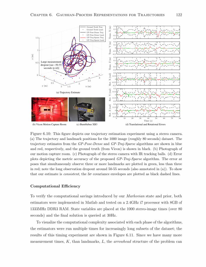
Chapter 6. Gaussian-Process Representations for Trajectories 122
Large measurement dropout [see ~50-55
seconds in (d)]
(b) Vicon Motion Capture Room (c) Bumblebee XB3 (d) Translational and Rotational Errors
(a) Trajectory Estimate
Figure 6.10: This figure depicts our trajectory estimation experiment using a stereo camera.
(a) The trajectory and landmark positions for the 1000 image (roughly 80 seconds) dataset. The
trajectory estimates from the GP-Pose-Dense and GP-Traj-Sparse algorithms are shown in blue
and red, respectively, and the ground truth (from Vicon) is shown in black. (b) Photograph of
our motion capture room. (c) Photograph of the stereo camera with IR tracking balls. (d) Error
plots depicting the metric accuracy of the proposed GP-Traj-Sparse algorithm. The error at
poses that simultaneously observe three or more landmarks are plotted in green, less than three
in red; note the long observation dropout around 50-55 seconds (also annotated in (a)). To show
that our estimate is consistent, the 3σ covariance envelopes are plotted as black dashed lines.
Computational Efficiency
To verify the computational savings introduced by our Markovian state and prior, both
estimators were implemented in Matlab and tested on a 2.4GHz i7 processor with 8GB of
1333MHz DDR3 RAM. State variables are placed at the 1000 stereo-image times (over 80
seconds) and the final solution is queried at 30Hz.
To visualize the computational complexity associated with each phase of the algorithms,
the estimators were run multiple times for increasingly long subsets of the dataset; the
results of this timing experiment are shown in Figure 6.11. Since we have many more
measurement times, K, than landmarks, L, the arrowhead structure of the problem can

Chapter 6. Gaussian-Process Representations for Trajectories 123
(a) Inverse kernel matrix construction time. (b) Optimization time per iteration.
(c) Interpolation time per additional query time. (d) Total computation time.
Figure 6.11: Comparison of the computation time required by both the GP-Pose-Dense
algorithm (as described by Tong et al. (2014)) and the GP-Traj-Sparse algorithm. The algorithms
were tested on varying dataset lengths. State variables were placed at the stereo image times
(roughly 15Hz) and then interpolated at 30Hz. The plots confirm the theoretical complexities of
the various algorithm phases. The total compute time required by the GP-Traj-Sparse algorithm
is linear in trajectory length. Note the linear-to-log scale transition in each plot.
be exploited by our GP-Traj-Sparse algorithm to solve the system in O(L3 + L2K) time,
using sparse lower-upper Cholesky decomposition and forward-backward passes. The
final solution is then queried J times (each in O(1) time), making the total algorithm
complexity O(L3 + L2K + J). Solving for only pose, the GP-Pose-Dense algorithm has a
half-size state vector, but a dense P−1; furthermore, no special form exists for P−1 and it
is computed by inverting the dense covariance matrix, P, which is a O(K3) operation.
Interpolation Quality
The last feature of our algorithm that we wish to demonstrate is its ability to predict the
state (and uncertainty) at times for which we do not have any measurements. To test this,
we repeated the batch estimation experiment, using the 80-second dataset, but removed a
block of 30 stereo images (spanning a roughly 2.3 second duration). Post optimization, we
interpolate the mean using (6.113) and the covariance using (6.127). The result, near the
subsection of interest, is shown in Figure 6.12. The estimated mean and covariance (at
the measurement times) are shown in blue. The interpolated mean (dashed red line) does
a reasonable job of predicting the intermediate behaviour shown by the ground truth (in
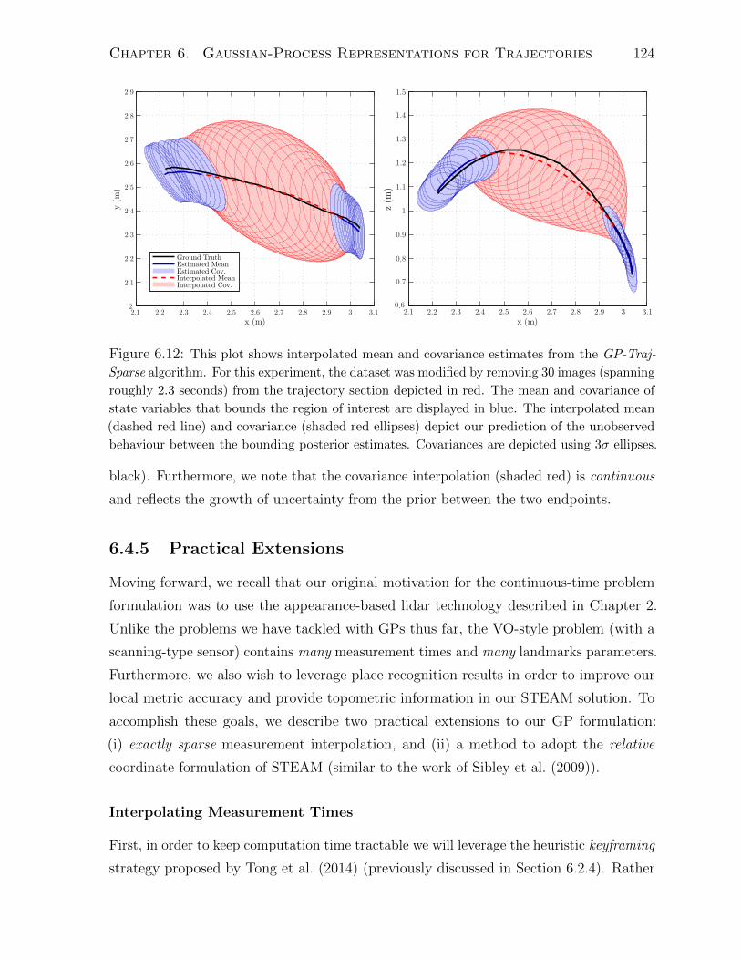
Chapter 6. Gaussian-Process Representations for Trajectories 124
Figure 6.12: This plot shows interpolated mean and covariance estimates from the GP-Traj-
Sparse algorithm. For this experiment, the dataset was modified by removing 30 images (spanning
roughly 2.3 seconds) from the trajectory section depicted in red. The mean and covariance of
state variables that bounds the region of interest are displayed in blue. The interpolated mean
(dashed red line) and covariance (shaded red ellipses) depict our prediction of the unobserved
behaviour between the bounding posterior estimates. Covariances are depicted using 3σ ellipses.
black). Furthermore, we note that the covariance interpolation (shaded red) is continuous
and reflects the growth of uncertainty from the prior between the two endpoints.
6.4.5 Practical Extensions
Moving forward, we recall that our original motivation for the continuous-time problem
formulation was to use the appearance-based lidar technology described in Chapter 2.
Unlike the problems we have tackled with GPs thus far, the VO-style problem (with a
scanning-type sensor) contains many measurement times and many landmarks parameters.
Furthermore, we also wish to leverage place recognition results in order to improve our
local metric accuracy and provide topometric information in our STEAM solution. To
accomplish these goals, we describe two practical extensions to our GP formulation:
(i) exactly sparse measurement interpolation, and (ii) a method to adopt the relative
coordinate formulation of STEAM (similar to the work of Sibley et al. (2009)).
Interpolating Measurement Times
First, in order to keep computation time tractable we will leverage the heuristic keyframing
strategy proposed by Tong et al. (2014) (previously discussed in Section 6.2.4). Rather

Chapter 6. Gaussian-Process Representations for Trajectories 125
than discretize the state trajectory, x(t), at the K measurement times, this strategy
advocates discretizing the state at a much coarser resolution of keytimes, N K.
Recalling the general form of our linearized observation model:
emkj(z + δz) ≈ ykj − g(T(tk), p`j ,ii )−Gx,kj δξ(tk)−G`,kj δ`j, (6.128)
we evaluate the observation model, g(·), and Jacobians, Gx,kj and G`,kj, by exploiting
the GP prediction equation, (6.113a), to calculate the interpolated transform, T(tk),
tn ≤ tk < tn+1. Since our trajectory state is no longer discretized at time tk, we must
also relate the ‘interpolated’ perturbation, δξ(tk), back to the discretized state, x; note
that our exactly sparse interpolation relies only on the temporally adjacent variables,
xn = Tn,i,$n, xn+1 = Tn+1,i,$n+1. Sparing the laborious details, we note that by
using our standard constraint-sensitive perturbations, along with the relationships we
derived in (6.118) and (6.121), we find that
δξ(tk) ≈[An(tk) Bn(tk)
]δxn+1 +
[Cn(tk) Dn(tk)
]δxn, tn ≤ tk < tn+1, (6.129)
with the analytical elements,
An(tk) :=J n(tk)(Ω11(tk) + 1
2Ω12(tk)$
fn+1
)J n(tn+1)−1,
Bn(tk) :=J n(tk)Ω12(tk)J n(tn+1)−1, Cn(tk) := T tk,tn −An(tk)T tn+1,tn , (6.130)
Dn(tk) :=J n(tk)Λ12(tk), where J n(t) := J (ln(T(t)T−1n,i)∨).
From a factor-graph perspective, we note that this causes our (originally) binary obser-
vation factors (dependent on xk and `j) to become ternary factors (dependent on xn,
xn+1, and `j). Concerning the sparsity of our Gauss-Newton problem, the (now) ternary
observation factors cause the top-left corner of the arrowhead matrix, GTR−1G, to become
block-tridiagonal (rather than block-diagonal). Since this new sparsity matches our
(already) block-tridiagonal prior term, F−TQ−1F−1, there is no adverse effect on the total
sparsity pattern. In fact, by estimating the state at N keytimes, N K, and exploiting
the sparsity of A``, the batch Gauss-Newton iterations become order O(N3 +N2L+K),
which is the same complexity as a traditional discrete-time SLAM problem (with N
keyframes and K measurements).
In this thesis we make the retrospective observation that the application of this
measurement interpolation scheme (in essence) transforms our nonparametric GP model
into a parametric one (using basis functions). Revisiting the general GP interpolation

Chapter 6. Gaussian-Process Representations for Trajectories 126
equation, (6.17a), from this new perspective (where the discretized state, x, does not
necessarily coincide with measurement times), we draw a similarity to the parametric
approach, discussed in Chapter 5, (5.1):
x(τ) = P(τ)P−1︸ ︷︷ ︸Ψ(t)
x + x(τ)− P(τ)P−1x︸ ︷︷ ︸time-varying constant
, (6.131)
where P(τ)P−1 can be viewed as a set of parametric basis functions, Ψ(t), weighted by state
vector x. Note that the additive, time-varying constant is simply zero for linear GP priors
that do not include control inputs (such as our piecewise, constant-velocity GP prior).
Unlike standard parametric approaches that tend to choose an interpolation scheme ad
hoc, we reiterate that the interpolation kernel, P(τ)P−1, can be derived directly from a
LTV SDE. We assert that this is a more principled way to arrive at a parametric model,
since the (now) physically motivated basis, Ψ(t), can also be viewed as a smoothness
constraint that enforces the optimal trajectory prediction between the keytimes (using
the continuous-time motion model).
To deepen this relationship, we derive the exact form of the basis for the white-noise-
on-acceleration prior used by our piecewise GP approach in Section 6.4.3. Recalling that
our LTI SDE results in a P(τ)P−1 with the two non-zero block-column entries
Λ(τ) = Φ(τ, tk)−Qk(τ)Φ(tk+1, τ)TQk(tk+1)−1Φ(tk+1, tk),
Ω(τ) = Qk(τ)Φ(tk+1, τ)TQk(tk+1)−1,
and analytical expressions for Φ(t, t′) and Qk(t), in (6.92) and (6.89), it follows that:
Λ(τ) =
[Λ11(τ) Λ12(τ)
Λ21(τ) Λ22(τ)
]=
[(2λ3 − 3λ2 + 1)1 ∆(λ3 − 2λ2 + λ)1
6∆
(λ2 − λ)1 (3λ2 − 4λ+ 1)1
](6.132a)
Ω(τ) =
[Ω11(τ) Ω12(τ)
Ω21(τ) Ω22(τ)
]=
[(3λ2 − 2λ3)1 ∆(λ3 − λ2)1
6∆
(λ− λ2)1 (3λ2 − 2λ)1
](6.132b)
where λ := τ−tntn+1−tn , ∆ := tn+1 − tn. Although this cubic interpolation scheme may not
seem special, we note that the top rows of coefficients form the exact expression used by
cubic Hermite splines and that the bottom rows are simply the derivatives. While we
advocate that the nonparametric approach to STEAM is more probabilistically justified,
we note that in situations where a parametric model must be used (e.g., for computational
reasons), it is motivating to generate the basis using the GP approach presented herein1.
1For the mathematically lazy, we suggest using cubic Hermite splines for parametric estimation sincethey are physically motivated, easy to implement, and efficient (with a local support of only two).

Chapter 6. Gaussian-Process Representations for Trajectories 127
Adopting the Relative Pose-Graph
In order to process large-scale loop closures in constant time (similar to the relative,
continuous-time method described in Chapter 5), we propose a hybrid approach to
incremental STEAM that maintains a relative state representation for the trajectory at
storage time (see Figure 6.13a), but converts to a privileged coordinate frame representation
to perform incremental, window-style batch optimizations (see Figure 6.13b). Recalling
that our trajectory state discretization, x, is already in the standard discrete-time form, we
note that it is trivial to convert our state parameterization to that of a relative pose-graph
(where we must also store body-centric velocities at the graph nodes). However, when it
comes to performing a window-style batch optimization (as described in Section 3.3.2), we
must choose to either: (i) re-factor the GP prior cost terms, in (6.96), and the interpolation
equations, in (6.113), to instead use the relative pose variables, Ttk+1,tk , or (ii) convert
the window of relative poses that we wish to optimize into a privileged coordinate frame.
Notably, the former approach can be used to augment an existing implementation of
discrete-time, relative SLAM (Sibley et al., 2009) with our exactly sparse set of GP
prior smoothing terms. However, we present two subtle advantages to taking the second
approach (which also apply to the discrete-time case).
The first advantage concerns the sparsity of the incremental batch estimation problems.
After selecting an active region of poses for the incremental batch optimization, it is
trivial to compound the relative pose chains back into a privileged root frame, F−→rob(tr),
where the root time, tr, aligns with one of the pose-graph node times, tk. Recalling that
the relative landmark parameters, p`j ,tjtj , are expressed in the frame where they are first
observed, F−→rob(tj), we note that the observation cost terms have the form:
emkj(z) = ykj − g(Ttk,tj p`j ,tjtj ) = ykj − g(Ttk,trT
−1tj ,tr
p`j ,tjtj ), (6.133)
where we have used the root frame to break the relative transforms, Ttk,tj , into exactly two
pose variables (rather than a chain of relative poses); by extension, this also results in a
much sparser set of Jacobians (for long feature tracks). Post optimization, the pose changes
can be extracted back into the relative storage format by using Ttk+1,tk = Ttk+1,trT−1tk,tr
.
Note that while even more sparsity can be obtained by temporarily expressing the
landmarks in the root frame, we find that the relative landmark formulation reduces the
number of required Gauss-Newton iterations dramatically. The intuition behind this is
that a global landmark representation (with a poor initial condition) can act as a damper
that causes the iterative trajectory updates to take small steps. In contrast, the global

Chapter 6. Gaussian-Process Representations for Trajectories 128
Trajectory Node Landmark
T3,2
2 T4,3
3 T5,4
4 T6,5
5 T7,6
6 7
T11,1010
T12,1111
T13,1212
T14,1313 14
T12,4 T13,5
2
11
4 5
(a) In order to store our trajectory state in a relative fashion, the standard relative pose-graph is augmented
to include body-centric velocity estimates at the nodes. Also, note that the landmark variables are stored
relative to the first frame in which they are observed.
Observation Factor Prior Factor Pose Constraint Root Pose
T2,4,2 T3,4,3 T4,r,4 T5,r,5 T6,r,6 T7,6,7
T10,11,10 T11,r,11 T12,r,12 T13,r,13Tr,r,14
211 4 5
Static Pose
(b) This figure illustrates a factor-graph view of our local batch optimization. Note that the active region
(shaded blue) of the relative pose-graph is transitioned to use the root pose as a privileged coordinate
frame. In contrast, static poses are expressed with respect to their nearest active leaf node; in essence,
these static regions form fixed submaps that float with the active pose to which they are constrained.
Ternary observation factors arise due to the landmarks being expressed in a relative fashion. Lastly, we
note that prior factors in parallel with a pose constraint still affect the active velocity variables.
Figure 6.13: This figure depicts our state representation at storage and optimization time.
structure of relative landmarks deforms ‘freely’ with changes to the trajectory estimate.
The second advantage of our approach involves the case where a loop exists within
the active sub-graph of relative poses that we are optimizing (i.e., when the active state
is over-parameterized). Rather than choose a minimal parameterization of relative states
to optimize, we note that converting to a set of privileged coordinates naturally enforces
a locally consistent solution.
In summary, our incremental STEAM technique operates in five stages: (i) perform a
breadth-first search from a root node to select an active region of the relative pose graph
to optimize, (ii) determine the active landmarks and the corresponding static region of
poses, (iii) concatenate the relative poses into a temporary, privileged state representation,
(iv) perform a local batch optimization using all of the relevant observation factors, as

Chapter 6. Gaussian-Process Representations for Trajectories 129
well as the GP prior factors between temporally adjacent trajectory states, and (v) push
updated pose, velocity, and landmark estimates back into the relative storage format.
6.4.6 Appearance-Based Lidar Experiment
In this section, we validate that our piecewise GP approach, combined with measurement
interpolation and our relative storage method, can be used to perform incremental
STEAM with high-rate asynchronous measurements in unstructured three-dimensional
terrain. Once again, we employ the use of our 1.1km appearance-based lidar dataset
described in Appendix A. Comparison is performed against an open-loop, discrete-time
solution and the closed-loop (parametric, relative) continuous-time method described in
Chapter 5. Furthermore, all compared estimators use the same SURF feature extractions,
preprocessed feature associations (i.e., outlier rejection), and loop closure proposals.
In contrast to the standard parametric approach, which focuses on proper knot spacing
to model smoothness (recall the tedious training in Chapter 5), our GP approach will
primarily rely on the prior model to prevent overfitting. Notably, spacing the keytimes
too far apart will still cause underfitting (i.e., over-smoothing); however, assuming that
the GP prior is well tuned, placing keytimes too close together will only have an adverse
affect on computational performance. Therefore, we must simply choose a knot spacing
large enough to enable online operation, but not too large as to over-smooth the solution.
For convenience, we choose to place a keytime at each lidar imagestack acquisition time
(a roughly half-second spacing) and found no adverse effects on accuracy. Concerning the
hyperparameters, we set our initial velocity prior, $0, to zero (with a high uncertainty),
and model QC as a diagonal matrix with its elements populated by Gaussians fit to
training data. Recalling that our GP prior approximates the nonlinear kinematic SDE in
(6.67), we note that the diagonal elements of QC can be interpreted as the variances of
the six body-centric acceleration (in rotation and translation).
Trajectory Estimation Performance
The open-loop trajectory estimates produced by our piecewise GP algorithm, GP-Traj-
Sparse, the parametric continuous-time algorithm from Chapter 5, Relative CT, and a
simple discrete-time implementation, Discrete, can be seen in Figure 6.14. The roughly
53 minute and 1.1km traversal contains 6880 intensity images, with 2,010,671 temporally
matched SURF features associated with 688,481 unique landmarks. As expected, both

Chapter 6. Gaussian-Process Representations for Trajectories 130
Start/End Start/End
Figure 6.14: Top and side views of the open-loop trajectory estimation results for the 1.1km
dataset. DGPS tracks are in black, the discrete-time estimate is in red, the parametric Relative
CT estimate (from Chapter 5) is in blue, and the GP-Traj-Sparse estimate (using measurement
interpolation) is in green.
continuous-time solutions perform much better than the discrete-time counterpart; note
that the discrete solution does not perform motion compensation in batch estimation, but
does leverage the motion-compensated RANSAC outlier rejection (described in Chapter 4).
Notably, both continuous-time solutions produce very similar results in the x-y plane; we
attribute the GP-Traj-Sparse algorithm’s improved elevation estimate to the trained GP
prior, which restricts large jumps in both the robo-centric z-axis and pitch velocity.
Since our continuous-time solutions also take advantage of loop-closures (in a topo-
metric sense), we are interested in comparing their local metric accuracy. Recalling the
ALARMS metric presented in Section 5.3.5, we provide a comparison in Figure 6.15.
Although the open-loop integration (OLI) result of our GP-Traj-Sparse algorithm is much
better that the OLI result of the Relative CT algorithm, we note that the improvement
in closed-loop integration (CLI) is marginal. This suggests that locally accurate results
can be obtained with either form of motion-compensation.
Despite the trajectory estimate of our GP approach being only marginally better that
the parametric method in Chapter 5, we note two other improvements: (i) a cleaner
state discretization, and (ii) faster computational performance. With respect to state
discretization, we note that being able to use the (fairly) standard relative pose-graph
storage (depicted in Figure 6.13) is much simpler than book-keeping overlapping basis
functions. Furthermore, it allows many existing discrete-time SLAM implementations to
be augmented with our GP prior smoothing terms and interpolation scheme. In contrast,
we note that using cubic B-splines (or other basis functions with a local support greater
than two) causes a tedious amount of book-keeping and special storage.
Although it is somewhat unfair to compare our computational results directly, since

Chapter 6. Gaussian-Process Representations for Trajectories 131
Figure 6.15: This figure shows the ALARMS error for a varying local region size. The continuous-
time estimates perform much better than the discrete-time counterpart. Furthermore, utilizing
the topological information to perform closed-loop integration results in the most accurate
local estimates. Notably, our GP-Traj-Sparse algorithm performs marginally better than the
parametric Relative CT algorithm.
the Relative CT method was implemented in Matlab and the GP-Traj-Sparse method
was implemented in C++, we note that the difference was substantial. In contrast to the
Relative CT algorithm, which required 1.6 hours of computation to process the 53 minute
dataset, our GP-Traj-Sparse method took a mere 15.6 minutes; coding language aside,
we note that this large speed up can be primarily attributed to the increased problem
sparsity and lack of burdensome numerical integration. The active window size used
in each algorithm was roughly the same (three seconds); using the relative pose-graph,
our GP approach performs a breadth-first search of depth six (where the keytimes are
spaced roughly half-seconds apart). Breaking the timing results down, the Relative
CT algorithm processed an average window in ∼0.84 seconds, while the GP-Traj-Sparse
method took only ∼0.14 seconds (which is fast enough to use the 2 Hz lidar scans online).
For context, we note that a typical window of six active frames (and another ∼10 static
frames) contains ∼2000 ‘visual’ measurements of ∼700 active landmarks. Furthermore, the
pose at each measurement time is individually interpolated and has a unique Jacobian
(∈ R6×(12+12)) that relates it to the adjacent keyframe poses and velocities. In comparison,
the computational cost of the GP smoothing factors is almost negligible.
Local Mapping Quality
Although it is common practice to validate SLAM algorithms using long trajectory plots
and error metrics based on (rough) GPS ground-truth, we note that the resolution of
these (typically) translation-only comparisons do not always indicate the usability of the

Chapter 6. Gaussian-Process Representations for Trajectories 132
(a) Before Motion Compensatation
(b) After Motion Compensatation
Figure 6.16: This figure depicts the effect of motion compensation for a sequence of lidar scans
acquired during continuous locomotion. In particular, we note that without compensating for
motion, a point cloud reprojection is susceptible to close objects being ‘echoed’, while the distant
reprojection is almost unusable. In contrast, by accounting for the temporal nature of the data
we are able to produce a very clean and consistent map.
localization and mapping for navigation purposes. Realistically, successful autonomous
systems do not depend on open-loop estimation for hundreds of meters at a time. In
order to gain intuition about an estimator’s ability to be used for obstacle detection and
safe, local navigation, it is interesting to inspect a dense (human-readable) map.
The first qualitative result that we wish to share about our continuous-time algorithm
is on the effects of motion compensation. In particular, we demonstrate the difference in
point-cloud construction, with and without using the continuous-time solution to properly

Chapter 6. Gaussian-Process Representations for Trajectories 133
Figure 6.17: This figure shows reprojected dense lidar data, coloured by elevation, from a local
region of our estimate that included loop closure. Furthermore, photographs of the experiment
provide context for the types of unstructured terrain we traversed with a scanning lidar sensor.
re-project lidar measurements from the spatiotemporal pose they were acquired at (see
Figure 6.16). Notably, without motion compensation our map is susceptible to ‘echoed’
ground planes and obstacles, as well as ‘blurry’ reprojections at distances greater than
∼5-10 meters. In contrast, our GP approach is able to produce a very clean point cloud.
The other qualitative result that we wish to share is a locally consistent point cloud
generated by reprojecting dense lidar data from an area involving loop closure (see
Figure 6.17). Notably, the reprojection uses lidar data from both passes of the area and
does not display any visible inconsistency.
6.5 Discussion
The GP-approach to trajectory estimation described in this chapter has provided a
theoretically pleasing batch optimization framework that is probabilistically founded on
continuous-time motion priors generated from stochastic models. Furthermore, it is clear

Chapter 6. Gaussian-Process Representations for Trajectories 134
Table 6.3: This table summarizes our sparsity conclusions with respect to the parameterization
of the robot state (while using a white-noise-on-acceleration prior). Concerning the standard
arrowhead matrix, GTR−1G, we report sparsity for the top-left corner (related to pose).
State Parameterization Sparsity of P Sparsity of GT R−1G,
pose only, T(t) dense block-diagonal
pose and velocity, T(t),$(t) block-tridiagonal block-diagonal
velocity only, $(t) block-tridiagonal dense (over integrated times)
(from a theoretical standpoint) that an accurately modelled GP prior eliminates the need
for ad hoc interpolation schemes or parametric models (such as B-splines). However, while
the purely nonparametric approach is both fast and effective for STEAM problems with
a small number of measurement times (or a small number of landmarks), we note that
current computing technology limits us from applying it to many of the interesting robotic
problems that we wish to solve (e.g., sweeping, motion-distorted lidar). In order to handle
high-rate or sweeping-type sensors in an online algorithm (with current technology), some
form of parametric model is required (such as the Hermite splines that arise from our GP
interpolation scheme). Nevertheless, the exactly sparse GP priors derived in this thesis
can be applied to many existing computationally tractable algorithms, such as keyframed
VO, and can be used to query the solution at other times of interest (post optimization).
Looking back on our GP formulation for SE(3), we note that the (desirable) nonlinear
SDE in (6.67) has a very simple linear form that depends on the state parameterization.
By marginalizing the pose variables and estimating only velocity (i.e., x(t) = $(t)),
the second half of the nonlinear SDE, $(t) = w(t) ∈ R6, becomes a LTI SDE for the
same problem. In fact, this is the exact prior model used by our parametric relative
continuous-time method in Chapter 5. However, we note that there is a cost associated
with marginalizing the pose variables: any pose-based observation (such as a visual
measurement) requires numerical integration of the velocity. Furthermore, the Jacobians
of the pose-based measurements also become dense over the length of velocity that must
be integrated. This finding concerning sparsity is similar in nature to the observation
of Barfoot et al. (2014), who found that marginalizing velocity variables caused an
acceleration-based prior to become dense over the pose variables. Table 6.3 summarizes
these conclusions; note that the most problem-sparsity is exploited by our GP-based
approach, which estimates both the position and velocity variables.

Chapter 6. Gaussian-Process Representations for Trajectories 135
6.6 Summary and Conclusions
In this chapter we have explored extensions to the nonparametric, Gaussian-process-
regression approach to batch continuous-time trajectory estimation. The approach was
originally proposed by Tong et al. (2012) and later matured by Barfoot et al. (2014)
to generate exactly sparse GP priors from linear time-varying SDEs. Within this field
of research, the contributions of this thesis are split into roughly two sections: (i) a
linearization methodology to generate exactly sparse GP priors from nonlinear time-
varying SDEs (for trajectories ∈ RN), and (ii) the application of this class of exactly
sparse GP priors to trajectories that belong to the matrix Lie group SE(3).
In the first portion of this chapter, we extended the work of Barfoot et al. (2014) by
showing how nonlinear time-varying SDEs can be used to generate an exactly sparse GP
prior. This is accomplished by linearizing the stochastic motion model about a continuous-
time operating point and then leveraging the existing linear procedures. Furthermore,
we perform an analysis of the complexities of this approach and explain how it can be
implemented in practice. We also show how both linear and nonlinear exactly sparse GP
priors can be exploited to improve the computational performance of data-driven hyper-
parameter training. Both our linearization methodology and data-driven hyperparameter
training are validated on a 2D indoor experimental dataset with accurate ground-truth.
These methods and results have previously appeared in Anderson et al. (2015a).
In summary, the contributions of this early work are:
1. A methodology to use NTV SDEs, driven by white noise, to generate an exactly
sparse GP prior for continuous-time trajectories that belong to a vectorspace.
2. An analysis of the complexities that arise from needing a continuous-time lineariza-
tion point. Specifically, we identify a circular dependence in the linearization,
propose a remedy that exploits the iterative nature of the estimation scheme, and
determine the minimal storage requirements.
3. An analysis of how data-driven hyperparameter training can also exploit the exactly
sparse nature of our GP priors.
4. An evaluation of both the nonlinear GP prior, formed from a NTV SDE, and the
data-driven hyperparameter training for a 2D mobile robot dataset.
In the later portion of the chapter, we investigate how the Markov property can be
exploited to make the GP-regression approach to STEAM efficient for bodies that are

Chapter 6. Gaussian-Process Representations for Trajectories 136
rotating and translating in 3D space. We first analyze how our linearization methodology
for vectorspaces can be extended to SE(3), for a (ideal) nonlinear prior, and then
demonstrated how a sequence of local, LTI SDEs can be used to form a close approximation.
Using this piecewise, linear GP prior, we propose a STEAM estimator for SE(3) that is
fast, singularity-free, and physically motivated. Furthermore, we demonstrate practical
extensions that allow us to use this technique with high-rate, motion-distorted lidar and
perform constant-time loop closure on a relative pose-graph. The methods are verified
experimentally for two different STEAM problems. Note that our exactly sparse GP prior
for SE(3), along with the stereo camera results, has previously appeared in Anderson
and Barfoot (2015); however, the relative extension and appearance-based lidar results
have not been previously published.
In summary, the contributions of this later work are:
1. A theoretical extension of our previous linearization methodology to generate an
exactly sparse GP prior from a NTV SDE that belongs to SE(3).
2. A piecewise GP prior that uses a sequence of local LTI SDEs to closely approximate
the desired NTV SDE (when velocity is near constant); the resultant GP-based
estimator is fast, singularity-free, and can be used to query the mean and covariance
of the posterior estimate at any time.
3. A description of the methodology we use to extend our GP estimator to the relative
coordinate formulation of STEAM.
4. An evaluation of our estimator’s accuracy, consistency, computational performance,
and ability to continuously interpolate both the mean and covariance functions,
using a stereo camera dataset.
5. An evaluation using lidar-style VO and place recognition over a 1.1 km traverse of
unstructured, three-dimensional terrain.
Notably, owing to the interesting parallel between the GP-regression approach to
STEAM and the standard discrete-time approach to SLAM, it is simple to apply our work
to most existing discrete-time batch SLAM implementations. Minimally, we note that
it is trivial to incorporate our three-dimensional GP prior factors into an existing batch
SLAM solution. Furthermore, this allows for the discrete-time posterior to be queried in
a continuous-time fashion; this may be useful for estimating a trajectory with a camera
and then reprojecting lidar data post optimization.

Chapter 7
Conclusion
In this chapter, we provide a short summary of the contributions and publications that
arose from the work presented in this thesis. Furthermore, we provide some narrative on
interesting directions for future work in the area of continuous-time trajectory estimation.
7.1 Summary of Contributions
Our motivation to work on batch continuous-time trajectory estimation originated from
the desire to use appearance-based lidar as a passive camera substitute (as described
in Chapter 2). Specifically, the original aim of this thesis was to extend the relative
coordinate formulation of batch discrete-time SLAM (as described in Chapter 3) to
estimate a continuous-time trajectory; we postulated that this would allow us to perform
incremental SLAM with high-rate asynchronous sensors, such as lidar – even at loop
closure. Along this journey we have learned much about batch continuous-time trajectory
estimation, made several contributions and publications towards the use of appearance-
based lidar for online STEAM, and what we hope are both theoretical and practical
contributions to the field of trajectory estimation for robotics.
The methods and experiments presented in Chapter 4, where we proposed a novel
RANSAC variant for motion-distorted sensors, first appeared in the publication:
• Anderson, S. and Barfoot, T. D. (2013a). RANSAC for motion-distorted 3D visual
sensors. In Proceedings of the International Conference on Intelligent Robots and
Systems (IROS), Tokyo, Japan.
The results were then combined with those of Chapter 5 and published in the article:
137

Chapter 7. Conclusion 138
• Anderson, S., MacTavish, K., and Barfoot, T. D. (2015b). Relative continuous-time
SLAM. International Journal of Robotics Research, 34(12):1453-1479.
In summary, the contributions of Chapter 4 are:
1. A temporally-sensitive adaptation of the vision-based RANSAC algorithm, using a
constant-velocity model to account for motion-distortion in 3D data.
2. A heuristic extension of the motion-compensated algorithm that improves computa-
tional performance without any large sacrifice to quality.
3. Derivation of the conditions for which our constant-velocity model can be solved.
4. An experimental validation of the algorithm, using SURF features extracted from a
6880 frame sequence of lidar intensity imagery.
The methods and experiments presented in Chapter 5, where we explored relative,
parametric continuous-time estimation, have appeared in two previous publications:
• Anderson, S. and Barfoot, T. D. (2013). Towards relative continuous-time SLAM.
In Proceedings of the IEEE International Conference on Robotics and Automation
(ICRA), Karlsruhe, Germany.
• Anderson, S., MacTavish, K., and Barfoot, T. D. (2015b). Relative continuous-time
SLAM. International Journal of Robotics Research, 34(12):1453-1479.
In summary, the contributions of Chapter 5 are:
1. A continuous-time adaptation of the relative-coordinate formulation of SLAM. We
demonstrate that by estimating the velocity profile of the robot, we can devise an
incremental SLAM solution that runs in constant time – even at loop closure.
2. An explanation of how to perform sliding-window-style estimation with basis func-
tions that have a local support greater than two.
3. An evaluation of the algorithm using lidar-style VO and appearance-based place
recognition over a 1.1 kilometer traverse of unstructured, three-dimensional terrain.
Most of the methods and experiments presented in Chapter 6, where we explored both
nonlinear and 3D extensions to a class of exactly sparse GP priors, have appeared in two
previous publications. First, the work of Barfoot et al. (2014) was extended by our work
on NTV SDEs and hyperparameter training for publication in a journal article:
• Anderson, S., Barfoot, T. D., Tong, C. H., and Sarkka, S. (2015a). Batch nonlinear
continuous-time trajectory estimation as exactly sparse gaussian process regression.
Autonomous Robots, special issue on Robotics Science and Systems, 39(3):221-238.
Chapter 7. Conclusion 139
Second, our exactly sparse GP prior for SE(3) was published in the proceedings of a
full-paper refereed conference, along with the stereo camera results:
• Anderson, S. and Barfoot, T. D. (2015). Full STEAM Ahead: Exactly sparse
gaussian process regression for batch continuous-time trajectory estimation on
SE(3). In Proceedings of the International Conference on Intelligent Robots and
Systems (IROS), pages 157-164, Hamburg, Germany.
Note that the relative extension and appearance-based lidar results have not been previ-
ously published. In summary, the contributions of Chapter 6 are:
1. A methodology to use NTV SDEs, driven by white noise, to generate an exactly
sparse GP prior for continuous-time trajectories that belong to a vectorspace.
2. An analysis of the complexities that arise from needing a continuous-time lineariza-
tion point and a description of the methods that allow us to implement a STEAM
estimator based on the nonlinear GP priors.
3. An analysis of how data-driven hyperparameter training can also exploit the exactly
sparse nature of our GP priors.
4. An evaluation of both the nonlinear GP prior, formed from a NTV SDE, and the
data-driven hyperparameter training for a 2D mobile robot dataset.
5. A theoretical extension of our linearization methodology to generate an exactly
sparse GP prior from a NTV SDE that belongs to SE(3).
6. A piecewise GP prior that uses a sequence of local LTI SDEs to closely approximate
the desired NTV SDE (when velocity is near constant).
7. A description of the methodology we use to extend our GP estimator to the relative
coordinate formulation of STEAM.
8. An evaluation of our estimator’s accuracy, consistency, computational performance,
and ability to continuously interpolate both the mean and covariance functions,
using a stereo camera dataset.
9. An evaluation of our estimator’s ability to perform lidar-style VO using a 1.1 km
traverse of unstructured, three-dimensional terrain.
7.2 Future Work
In this section we discuss possible avenues of future work. The suggestions are partitioned
into those that concern the parametric and nonparametric approaches to STEAM.
The biggest challenge for the parametric approach to trajectory estimation is choosing
a knot spacing that will reliably fit the true motion of the vehicle. Although we propose

Chapter 7. Conclusion 140
that a more realistic motion prior can help alleviate the chance of overfitting, we note
that knot spacing is a more intuitive and predictable method for an engineer to tune
the smoothness of a trajectory curve. Along this line of thought, we make the following
suggestions for possible extensions to the parametric approach:
1. The work of Oth et al. (2013) proposes using a normalized innovation squared (NIS)
test to determine when higher knot resolution is required. This avenue is very
promising, but it is not clear that a naive implementation of this approach will be
robust to outliers. Further work is required in this area.
2. An alternative approach is to try and use a priori information to choose a knot
spacing. For example, one could characterize the behaviour of a specific vehicle and
then choose the knot spacing based on the commanded control inputs.
Our suggestions for the nonparametric approach are primarily comprised of improvements
and extensions to the GP prior model:
1. The most straightforward extension of our 3D approach would be to consider other
kinematic models that might be more suitable for non-ground vehicles; for example,
one might expect the primary disturbances on quadrotor control to be more prevalent
in an inertial frame, rather than the body-centric frame.
2. Reintroducing the control inputs into our piecewise GP prior could be beneficial.
However, we note that wheel slip and other unanticipated forces prevent us from
trusting the control inputs too heavily. An interesting exercise would be to model the
smoothing term, QC , as a time-varying function that takes the control inputs as a
parameter (e.g., when the control inputs are zero, we expect almost no acceleration).
3. In general, it would be interesting to exploit as much a priori knowledge in the
GP prior as possible. For example, dynamical models can be used by including
vehicle mass, the gravity vector, motor torques, and even terrain interactions. The
surface upon which a ground vehicle drives is a relatively unexploited prior in
three-dimensions. Given a model of the terrain (e.g., using lidar scans) one could
include cost terms that penalize the pose estimate if it tries to ‘float away’.
These avenues of future work represent some of the next steps in maturing the use of
continuous-time trajectory representations for robotic localization. It is my belief that
this field of research is very promising and it is my hope that these types of techniques
become more widely adopted in the many fields of robotic state estimation.

Appendix A
Appearance-Based Lidar Dataset
In order to generate repeatable experimental results for this thesis, the appearance-based
lidar experiments conducted by McManus et al. (2012) were packaged into the publicly
available1 Gravel Pit Lidar-Intensity Imagery Dataset (Anderson et al., 2012). The general
pipeline used to process lidar data in these experiments is reviewed in Chapter 2. The
experiments used a ROC6 field robot, equipped with an Autonosys LVC0702 lidar, to
capture intensity, range, azimuth, elevation, and timestamp images, with a resolution of
480× 360, at 2Hz; the hardware configuration is presented in Figure 2.1(a) and typical
intensity/range images are shown in Figure 2.2. The purpose of this appendix is to provide
additional detail on the data products, models, and post-processed results used by the
experimental results in this thesis.
1The dataset is available at http://asrl.utias.utoronto.ca/datasets/abl-sudbury/, along withdetailed descriptions of the various post-processed data products and coordinate frames.
Figure A.1: The Ethier Sand and Gravel pit in Sudbury, Ontario, Canada.
141
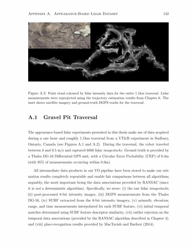
Appendix A. Appearance-Based Lidar Dataset 142
Figure A.2: Point cloud coloured by lidar intensity data for the entire 1.1km traversal. Lidar
measurements were reprojected using the trajectory estimation results from Chapter 6. The
inset shows satellite imagery and ground-truth DGPS tracks for the traversal.
A.1 Gravel Pit Traversal
The appearance-based lidar experiments presented in this thesis make use of data acquired
during a one hour and roughly 1.1km traversal from a VT&R experiment in Sudbury,
Ontario, Canada (see Figures A.1 and A.2). During the traversal, the robot traveled
between 0 and 0.5 m/s and captured 6880 lidar imagestacks. Ground truth is provided by
a Thales DG-16 Differential GPS unit, with a Circular Error Probability (CEP) of 0.4m
(with 95% of measurements occurring within 0.9m).
All intermediate data products in our VO pipeline have been stored to make our esti-
mation results completely repeatable and enable fair comparisons between all algorithms;
arguably, the most important being the data associations provided by RANSAC (since
it is not a deterministic algorithm). Specifically, we store: (i) the raw lidar imagestacks,
(ii) post-processed 8-bit intensity images, (iii) DGPS measurements from the Thales
DG-16, (iv) SURF extracted from the 8-bit intensity imagery, (v) azimuth, elevation,
range, and time measurements interpolated for each SURF feature, (vi) initial temporal
matches determined using SURF feature descriptor similarity, (vii) outlier rejection on the
temporal data associations (provided by the RANSAC algorithm described in Chapter 4),
and (viii) place-recognition results provided by MacTavish and Barfoot (2014).

Appendix A. Appearance-Based Lidar Dataset 143
A.2 Measurement Model
Owing to the nature of the ray-like measurements (i.e. azimuth, elevation, and range), a
spherical observation model was used for the vision-based algorithms in Chapters 4, 5,
and 6. Noting the observation-model linearization performed in Chapter 3 – equation
(3.63) – we define the following spherical model for our lidar SURF measurements:
k(p`,ss ) :=
atan2(ε2,
√ε2
1 + ε23)
atan2(ε3, ε1)√ε21+ε22+ε23
η
, p`,ss =
[ε
η
], (A.1)
where p`,ss is the homogeneous coordinate for the position of point `, expressed in sensor
frame F−→s, and k(·) is the nonlinear sensor model that transforms the point into the
spherical sensor space. The observation model Jacobian, Kkj, needed to complete the
linearization is therefore
Kkj :=
− ε1 ε2
(ε21+ε22+ε23)√ε21+ε23
√ε21+ε23
ε21+ε22+ε23− ε2 ε3
(ε21+ε22+ε23)√ε21+ε23
0
− ε3ε21+ε22
0 ε1ε21+ε22
0
ε1
η√ε21+ε22+ε23
ε2
η√ε21+ε22+ε23
ε3
η√ε21+ε22+ε23
−√ε21+ε22+ε23η2
. (A.2)
Lastly, we note that in order to use a simple spherical model for our measurements,
the raw azimuth, elevation, and range measurements, y′kj, require an intrinsic calibration
due to the true nature of the sensor (see Figure 2.1(b)). This is accomplished by using
the generalized distortion model presented by Dong et al. (2013). The augmented (i.e.
undistorted) spherical measurement, ykj, is found using the model:
ykj = y′kj + Ψ(α′, β′)c, y′kj =[α′ β′ r′
]T, (A.3)
where Ψ(α′, β′) is a set of basis functions (e.g. grid-based bilinear interpolation) that
takes the raw azimuth and elevation as inputs, and c is a set of pre-optimized weighting
coefficients that determine the additive correction.
A.3 Place Recognition
Loop-closure proposals were generated for the Chapter 5 and 6 experiments by using
the place-recognition algorithm proposed by MacTavish and Barfoot (2014). Based
on FAB-MAP (Cummins and Newman, 2008), the augmented algorithm describes and

Appendix A. Appearance-Based Lidar Dataset 144
0 0.1 0.2 0.3 0.4 0.5 0.6 0.7 0.8 0.9 10
0.2
0.4
0.6
0.8
1
Recall
Pre
cisi
on
1163264Selected
Figure A.3: This figure shows the precision-
recall curve of place recognition for different
image-group sizes. Note the significant im-
provement of group matching over the single-
image representation. The selected group size
of 32 and threshold of p ≥ 0.85 resulted in
61% precision and 25% recall.
Loops 1-2
Loop 3
Loops 4-7
Loops 8-9
Figure A.4: This figure shows the loop closure
proposals overlaid onto the GPS data. The
nine accepted loop closures are shown in green,
while the rejected loop closures are shown in
red. Note that the blue trajectory segment
was used for training, and was not evaluated
for loop closures.
compares groups of images; loop closures are proposed by computing the likelihood that
a query intensity image (or group of images) came from each previously visited location.
Due to the (poor) quality of features extracted from our motion-distorted lidar intensity
imagery we found that this modification was necessary to get reasonable place-recognition
performance (see Figure A.3).
In order to geometrically validate the proposed loop closures, the SURF feature
measurements from the blocks of 32 images are undistorted into a privileged coordinate
frame (using the continuous-time trajectory solutions from Chapters 5 and 6). A standard
RANSAC algorithm is then run to find a transformation between the two temporal
segments that validates the loop closure; of the proposed 21 matches, seen in Figure A.4,
the nine shown in green were accepted (in both STEAM experiments).

Bibliography
Absil, P.-A., Mahony, R., and Sepulchre, R. (2009). Optimization algorithms on matrixmanifolds. Princeton University Press.
Ait-Aider, O., Andreff, N., Lavest, J., and Martinet, P. (2006). Simultaneous object poseand velocity computation using a single view from a rolling shutter camera. ComputerVision–ECCV 2006, pages 56–68.
Ait-Aider, O. and Berry, F. (2009). Structure and kinematics triangulation with a rollingshutter stereo rig. In Computer Vision, 2009 IEEE 12th International Conference on,pages 1835–1840. IEEE.
Anderson, S. and Barfoot, T. D. (2013a). Ransac for motion-distorted 3d visual sensors.In IEEE/RSJ International Conference on Intelligent Robots and Systems (IROS),Tokyo, Japan.
Anderson, S. and Barfoot, T. D. (2013b). Towards relative continuous-time slam. InProceedings of the IEEE International Conference on Robotics and Automation (ICRA),Karlsruhe, Germany.
Anderson, S. and Barfoot, T. D. (2015). Full steam ahead: Exactly sparse gaussian processregression for batch continuous-time trajectory estimation on se(3). In Proceedings ofthe IEEE/RSJ International Conference on Intelligent Robots and Systems (IROS),pages 157–164, Hamburg, Germany.
Anderson, S., Barfoot, T. D., Tong, C. H., and Sarkka, S. (2015a). Batch nonlinearcontinuous-time trajectory estimation as exactly sparse gaussian process regression.Autonomous Robots, special issue on “Robotics Science and Systems”, 39(3):221–238.
Anderson, S., Dellaert, F., and Barfoot, T. D. (2014). A hierarchical wavelet decompositionfor continuous-time slam. In Proceedings of the IEEE International Conference onRobotics and Automation (ICRA), Hong Kong, China.
Anderson, S., MacTavish, K., and Barfoot, T. D. (2015b). Relative continuous-time slam.International Journal of Robotics Research, 34(12):1453–1479.
Anderson, S., McManus, C., Dong, H., Beerepoot, E., and Barfoot, T. D. (2012). Thegravel pit lidar-intensity imagery dataset. Technical Report ASRL-2012-ABL001,UTIAS.
145

BIBLIOGRAPHY 146
Arun, K. S., Huang, T. S., and Blostein, S. D. (1987). Least-squares fitting of two3-d point sets. Pattern Analysis and Machine Intelligence, IEEE Transactions on,(5):698–700.
Barfoot, T. D. (2016). State Estimation for Robotics: A Matrix-Lie-Group Approach.Draft in preparation for publication by Cambridge University Press.
Barfoot, T. D. and Furgale, P. T. (2014). Associating uncertainty with three-dimensionalposes for use in estimation problems. IEEE Transactions on Robotics.
Barfoot, T. D., McManus, C., Anderson, S., Dong, H., Beerepoot, E., Tong, C. H., Furgale,P., Gammell, J. D., and Enright, J. (2013). Into darkness: Visual navigation basedon a lidar-intensity-image pipeline. In Proceedings of the International Symposium onRobotics Research (ISRR), Singapore.
Barfoot, T. D., Tong, C. H., and Sarkka, S. (2014). Batch continuous-time trajectoryestimation as exactly sparse gaussian process regression. In Proceedings of Robotics:Science and Systems (RSS), Berkeley, USA.
Bay, H., Tuytelaars, T., and Van Gool, L. (2006). Surf: Speeded up robust features.Computer Vision–ECCV 2006, pages 404–417.
Bell, B. M. (1994). The iterated kalman smoother as a Gauss-Newton method. SIAMJournal on Optimization, 4(3):626–636.
Berczi, L.-P., Posner, I., and Barfoot, T. D. (2015). Learning to assess terrain from humandemonstration using an introspective gaussian-process classifier. In Proceedings of theIEEE International Conference on Robotics and Automation (ICRA), pages 3178–3185,Seattle, Washington.
Besl, P. J. and McKay, N. D. (1992). Method for registration of 3-d shapes. In Robotics-DLtentative, pages 586–606. International Society for Optics and Photonics.
Bibby, C. and Reid, I. (2010). A hybrid slam representation for dynamic marine en-vironments. In Proceedings of the IEEE International Conference on Robotics andAutomation (ICRA), pages 257–264. IEEE.
Bosse, M. and Zlot, R. (2009). Continuous 3d scan-matching with a spinning 2d laser. InProceedings of the IEEE International Conference on Robotics and Automation (ICRA),pages 4312–4319. IEEE.
Bosse, M., Zlot, R., and Flick, P. (2012). Zebedee: Design of a spring-mounted 3-drange sensor with application to mobile mapping. IEEE Transactions on Robotics,28(5):1104–1119.
Brown, D. C. (1958). A solution to the general problem of multiple station analyticalstereotriangulation. RCA-MTP data reduction tech. report no. 43, Patrick AirforceBase.

BIBLIOGRAPHY 147
Calonder, M., Lepetit, V., Strecha, C., and Fua, P. (2010). Brief: Binary robust indepen-dent elementary features. Computer Vision–ECCV 2010, pages 778–792.
Chirikjian, G. S. (2009). Stochastic Models, Information Theory, and Lie Groups: ClassicalResults and Geometric Methods, volume 1-2. Birkhauser, New York.
Chirikjian, G. S. and Kyatkin, A. B. (2016). Harmonic Analysis for Engineers and AppliedScientists: Updated and Expanded Edition. Courier Dover Publications.
Chli, M. and Davison, A. J. (2008). Active matching. In Computer Vision–ECCV 2008,pages 72–85. Springer.
Churchill, W. and Newman, P. (2012). Practice makes perfect? managing and leveragingvisual experiences for lifelong navigation. In Proceedings of the IEEE InternationalConference on Robotics and Automation, pages 4525–4532. IEEE.
Churchill, W. and Newman, P. (2013). Experience-based Navigation for Long-termLocalisation. The International Journal of Robotics Research (IJRR).
Cummins, M. and Newman, P. (2008). Fab-map: Probabilistic localization and mapping inthe space of appearance. The International Journal of Robotics Research, 27(6):647–665.
Davison, A. J., Reid, I. D., Molton, N. D., and Stasse, O. (2007). MonoSLAM: Real-timesingle camera SLAM. IEEE T. PAMI, 29(6):1052–1067.
Deisenroth, M. P., Turner, R., Huber, M., Hanebeck, U. D., and Rasmussen, C. E. (2012).Robust filtering and smoothing with Gaussian processes. IEEE T. Automatic Control,57:1865–1871.
Dellaert, F. and Kaess, M. (2006). Square root sam: Simultaneous localization andmapping via square root information smoothing. The International Journal of RoboticsResearch, 25(12):1181–1203.
Dong, H., Anderson, S., and Barfoot, T. D. (2013). Two-axis scanning lidar geometriccalibration using intensity imagery and distortion mapping. In Proceedings of the IEEEInternational Conference on Robotics and Automation (ICRA), Karlsruhe, Germany.
Dong, H. and Barfoot, T. (2011). Pose interpolation for bundle adjustment.
Dong, H. and Barfoot, T. D. (2012). Lighting-invariant visual odometry using lidarintensity imagery and pose interpolation. In Proceedings of the International Conferenceon Field and Service Robotics (FSR), Matsushima, Japan.
Ferris, B., Fox, D., and Lawrence, N. (2007). Wifi-SLAM using Gaussian process latentvariable models. In Proc. IJCAI.
Fischler, M. and Bolles, R. (1981). Random sample consensus: a paradigm for modelfitting with applications to image analysis and automated cartography. Communicationsof the ACM, 24(6):381–395.
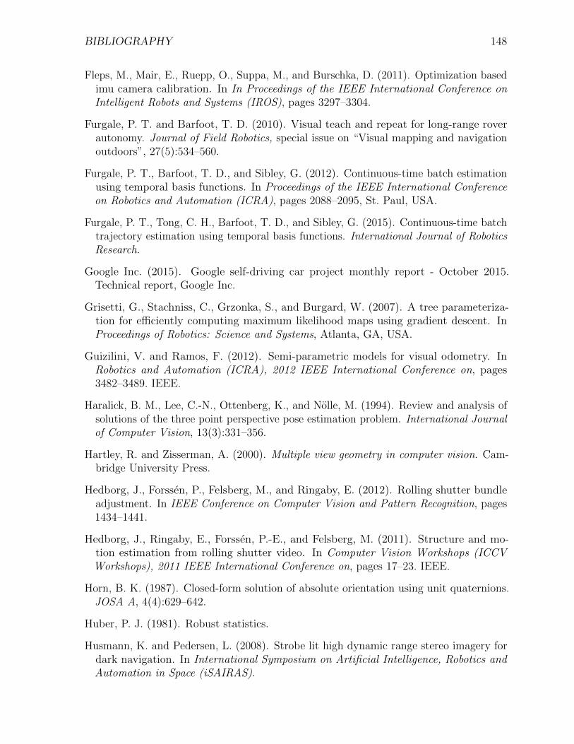
BIBLIOGRAPHY 148
Fleps, M., Mair, E., Ruepp, O., Suppa, M., and Burschka, D. (2011). Optimization basedimu camera calibration. In In Proceedings of the IEEE International Conference onIntelligent Robots and Systems (IROS), pages 3297–3304.
Furgale, P. T. and Barfoot, T. D. (2010). Visual teach and repeat for long-range roverautonomy. Journal of Field Robotics, special issue on “Visual mapping and navigationoutdoors”, 27(5):534–560.
Furgale, P. T., Barfoot, T. D., and Sibley, G. (2012). Continuous-time batch estimationusing temporal basis functions. In Proceedings of the IEEE International Conferenceon Robotics and Automation (ICRA), pages 2088–2095, St. Paul, USA.
Furgale, P. T., Tong, C. H., Barfoot, T. D., and Sibley, G. (2015). Continuous-time batchtrajectory estimation using temporal basis functions. International Journal of RoboticsResearch.
Google Inc. (2015). Google self-driving car project monthly report - October 2015.Technical report, Google Inc.
Grisetti, G., Stachniss, C., Grzonka, S., and Burgard, W. (2007). A tree parameteriza-tion for efficiently computing maximum likelihood maps using gradient descent. InProceedings of Robotics: Science and Systems, Atlanta, GA, USA.
Guizilini, V. and Ramos, F. (2012). Semi-parametric models for visual odometry. InRobotics and Automation (ICRA), 2012 IEEE International Conference on, pages3482–3489. IEEE.
Haralick, B. M., Lee, C.-N., Ottenberg, K., and Nolle, M. (1994). Review and analysis ofsolutions of the three point perspective pose estimation problem. International Journalof Computer Vision, 13(3):331–356.
Hartley, R. and Zisserman, A. (2000). Multiple view geometry in computer vision. Cam-bridge University Press.
Hedborg, J., Forssen, P., Felsberg, M., and Ringaby, E. (2012). Rolling shutter bundleadjustment. In IEEE Conference on Computer Vision and Pattern Recognition, pages1434–1441.
Hedborg, J., Ringaby, E., Forssen, P.-E., and Felsberg, M. (2011). Structure and mo-tion estimation from rolling shutter video. In Computer Vision Workshops (ICCVWorkshops), 2011 IEEE International Conference on, pages 17–23. IEEE.
Horn, B. K. (1987). Closed-form solution of absolute orientation using unit quaternions.JOSA A, 4(4):629–642.
Huber, P. J. (1981). Robust statistics.
Husmann, K. and Pedersen, L. (2008). Strobe lit high dynamic range stereo imagery fordark navigation. In International Symposium on Artificial Intelligence, Robotics andAutomation in Space (iSAIRAS).

BIBLIOGRAPHY 149
Jazwinski, A. H. (1970). Stochastic Processes and Filtering Theory. Academic, New York.
Jia, C. and Evans, B. L. (2012). Probabilistic 3-d motion estimation for rolling shuttervideo rectification from visual and inertial measurements. In Proc. IEEE Int. Workshopon Multimedia Signal Processing.
Johnson, A. E., Goldberg, S. B., Cheng, Y., and Matthies, L. H. (2008). Robust andefficient stereo feature tracking for visual odometry. In IEEE International Conferenceon Robotics and Automation, pages 39–46. IEEE.
Julier, S. J. and Uhlmann, J. K. (1997). New extension of the kalman filter to nonlinearsystems. In AeroSense’97, pages 182–193. International Society for Optics and Photonics.
Kaess, M., Johannsson, H., Roberts, R., Ila, V., Leonard, J. J., and Dellaert, F. (2012).iSAM2: Incremental smoothing and mapping using the Bayes tree. IJRR, 31(2):217–236.
Kaess, M., Ranganathan, A., and Dellaert, R. (2008). iSAM: Incremental smoothing andmapping. IEEE TRO, 24(6):1365–1378.
Kalman, R. E. (1960). A new approach to linear filtering and prediction problems.Transactions of the ASME–Journal of Basic Engineering, 82(Series D):35–45.
Kalman, R. E. and Bucy, R. S. (1961). New results in linear filtering and predictiontheory. Transactions of the ASME–Journal of Basic Engineering, 83(3):95–108.
Kim, M.-J., Kim, M.-S., and Shin, S. Y. (1995). A general construction scheme for unitquaternion curves with simple high order derivatives. In Proceedings of the 22nd annualconference on Computer graphics and interactive techniques, pages 369–376. ACM.
Ko, J. and Fox, D. (2009). GP-BayesFilters: Bayesian filtering using Gaussian processprediction and observation models. Autonomous Robots, 27(1):75–90.
Ko, J. and Fox, D. (2011). Learning GP-BayesFilters via Gaussian process latent variablemodels. Auton. Robots, 30(1):3–23.
Konolige, K. (2010). Sparse sparse bundle adjustment. In Proceedings of the BritishMachine Vision Conference, pages 1–11.
Konolige, K., Agrawal, M., and Sola, J. (2007). Large-scale visual odometry for roughterrain. In Proceedings of the International Symposium on Robotics Research (ISRR),pages 201–212.
Konolige, K., Bowman, J., Chen, J., Mihelich, P., Calonder, M., Lepetit, V., and Fua, P.(2010). View-based maps. The International Journal of Robotics Research, 29(8):941.
Lawrence, N. (2003). Gaussian process latent variable models for visualization of highdimensional data. In Proc. NIPS.

BIBLIOGRAPHY 150
Leutenegger, S., Chli, M., and Siegwart, R. Y. (2011). Brisk: Binary robust invariantscalable keypoints. In Computer Vision (ICCV), 2011 IEEE International Conferenceon, pages 2548–2555. IEEE.
Levenberg, K. (1944). A method for the solution of certain non–linear problems in leastsquares.
Levinson, J. S. (2011). Automatic laser calibration, mapping, and localization for au-tonomous vehicles. Stanford University.
Longuet-Higgins, H. (1981). A computer algorithm for reconstructing a scene from twoprojections. Nature, 293:133–135.
Lovegrove, S., Patron-Perez, A., and Sibley, G. (2013). Spline fusion: A continuous-timerepresentation for visual-inertial fusion with application to rolling shutter cameras.British Machine Vision Conference (BMVC13).
Lowe, D. (2004). Distinctive image features from scale-invariant keypoints. Internationaljournal of computer vision, 60(2):91–110.
Lu, F. and Milios, E. (1997). Globally consistent range scan alignment for environmentmapping. Auton. Robots, 4(4):333–349.
Lucas, B. D. and Kanade, T. (1981). An iterative image registration technique with anapplication to stereo vision. In Proceedings of the 7th international joint conference onArtificial intelligence.
MacTavish, K. and Barfoot, T. D. (2014). Towards hierarchical place recognition forlong-term autonomy. In Proceedings of the IEEE International Conference on Roboticsand Automation workshop on “Visual Place Recognition in Changing Environments”,Hong Kong, China.
Magnusson, M., Lilienthal, A., and Duckett, T. (2007). Scan registration for autonomousmining vehicles using 3d-ndt. Journal of Field Robotics, 24(10):803–827.
Maimone, M., Cheng, Y., and Matthies, L. (2007). Two years of visual odometry on themars exploration rovers. Journal of Field Robotics, 24(3):169–186.
Maimone, M., Johnson, A., Cheng, Y., Willson, R., and Matthies, L. (2006). Autonomousnavigation results from the mars exploration rover (mer) mission. Experimental RoboticsIX, pages 3–13.
Marquardt, D. W. (1963). An algorithm for least-squares estimation of nonlinear parame-ters. Journal of the Society for Industrial & Applied Mathematics, 11(2):431–441.
Matthies, L., Maimone, M., Johnson, A., Cheng, Y., Willson, R., Villalpando, C.,Goldberg, S., Huertas, A., Stein, A., and Angelova, A. (2007). Computer vision onmars. International Journal of Computer Vision.

BIBLIOGRAPHY 151
Matthies, L. and Shafer, S. (1987). Error modeling in stereo navigation. IEEE Journal ofRobotics and Automation, 3(3).
Matthies, L. H. (1989). Dynamic Stereo Vision. PhD thesis, Pittsburgh, PA, USA.AAI9023429.
McManus, C., Furgale, P. T., and Barfoot, T. D. (2011). Towards appearance-basedmethods for lidar sensors. In Proceedings of the IEEE International Conference onRobotics and Automation (ICRA), pages 1930–1935, Shanghai, China.
McManus, C., Furgale, P. T., and Barfoot, T. D. (2013). Towards lighting-invariant visualnavigation: An appearance-based approach using scanning laser-rangefinders. Roboticsand Autonomous Systems, 61:836–852.
McManus, C., Furgale, P. T., Stenning, B. E., and Barfoot, T. D. (2012). Visual teachand repeat using appearance-based lidar. In Proceedings of the IEEE InternationalConference on Robotics and Automation (ICRA), pages 389–396, St. Paul, USA.
Moravec, H. (1980). Obstacle avoidance and navigation in the real world by a seeing robotrover. In tech. report CMU-RI-TR-80-03, Robotics Institute, Carnegie Mellon Universityand doctoral dissertation, Stanford University, number CMU-RI-TR-80-03. Availableas Stanford AIM-340, CS-80-813 and republished as a Carnegie Mellon UniversityRobotics Institue Technical Report to increase availability.
Murray, R. M., Li, Z., and Sastry, S. (1994). A mathematical introduction to roboticmanipulation. Boca Raton, FL: CRC.
Neira, J., Tardos, J. D., Horn, J., and Schmidt, G. (1999). Fusing range and intensityimages for mobile robot localization. IEEE Transactions on Robotics and Automation,15:76–84.
Nister, D. (2004). An efficient solution to the five-point relative pose problem. PatternAnalysis and Machine Intelligence, IEEE Transactions on, 26(6):756–770.
Nuchter, A., Lingemann, K., Hertzberg, J., and Surmann, H. (2007). 6d slam-3d mappingoutdoor environments. Journal of Field Robotics, 24(8-9):699–722.
Olson, E., Leonard, J., and Teller, S. (2006). Fast iterative alignment of pose graphs withpoor initial estimates. In Proceedings of the IEEE International Conference on Roboticsand Automation, pages 2262–2269. IEEE.
Oth, L., Furgale, P. T., Kneip, L., and Siegwart, R. (2013). Rolling shutter cameracalibration. In Proc. of The IEEE International Conference on Computer Vision andPattern Recognition (CVPR), Portland, USA.
Pathak, K., Birk, A., Vaskevicius, N., Pfingsthorn, M., Schwertfeger, S., and Poppinga, J.(2010). Online three-dimensional slam by registration of large planar surface segmentsand closed-form pose-graph relaxation. Journal of Field Robotics, 27(1):52–84.

BIBLIOGRAPHY 152
Pomerleau, F., Colas, F., and Siegwart, R. (2015). A Review of Point Cloud RegistrationAlgorithms for Mobile Robotics. Foundations and Trends in Robotics (FnTROB),4(1):1–104.
Powell, M. J. (1970). A hybrid method for nonlinear equations. Numerical methods fornonlinear algebraic equations, 7:87–114.
Ranganathan, P. and Olson, E. (2012). Gaussian process for lens distortion modeling. InIEEE/RSJ International Conference on Intelligent Robots and Systems (IROS), pages3620–3625. IEEE.
Rankin, A. L., Huertas, A., and Matthies, L. H. (2007). Night-time negative obstacledetection for off-road autonomous navigation. In Defense and Security Symposium,pages 656103–656103. International Society for Optics and Photonics.
Rasmussen, C. E. and Williams, C. K. I. (2006). Gaussian Processes for Machine Learning.MIT Press, Cambridge, MA.
Rosen, D., Huang, G., and Leonard, J. J. (2014). Inference over heterogeneous finite-/infinite-dimensional systems using factor graphs and Gaussian processes. In Proceedingsof the IEEE International Conference on Robotics and Automation, pages 1261–1268.
Rosten, E. and Drummond, T. (2006). Machine learning for high-speed corner detection.In Computer Vision–ECCV 2006, pages 430–443. Springer.
Rublee, E., Rabaud, V., Konolige, K., and Bradski, G. (2011). Orb: An efficient alternativeto sift or surf. In International Conference on Computer Vision, Barcelona.
Sarkka, S. (2006). Recursive Bayesian Inference on Stochastic Differential Equations.PhD thesis, Helsinki Uni. of Technology.
Sibley, G., Matthies, L., and Sukhatme, G. (2008). A sliding window filter for incrementalslam. In Unifying perspectives in computational and robot vision, pages 103–112.Springer.
Sibley, G., Mei, C., Reid, I., and Newman, P. (2009). Adaptive relative bundle adjustment.In Proceedings of Robotics: Science and Systems, Seattle, USA.
Sibley, G., Mei, C., Reid, I., and Newman, P. (2010). Vast-scale outdoor navigation usingadaptive relative bundle adjustment. The International Journal of Robotics Research,29(8):958.
Smith, R. C., Self, M., and Cheeseman, P. (1990). Estimating uncertain spatial relation-ships in robotics. In Cox, I. J. and Wilfong, G. T., editors, Autonomous Robot Vehicles,pages 167–193. Springer Verlag, New York.
Sommer, H., Forbes, J. R., Siegwart, R., and Furgale, P. (2015). Continuous-timeestimation of attitude using b-splines on lie groups. Journal of Guidance, Control, andDynamics, pages 1–20.

BIBLIOGRAPHY 153
Stenning, B. E., McManus, C., and Barfoot, T. D. (2013). Planning using a network ofreusable paths: A physical embodiment of a rapidly exploring random tree. Journal ofField Robotics, special issue on “Space Robotics”, 30(6):916–950.
Strasdat, H., Montiel, J. M. M., and Davison, A. J. (2010). Real-time monocular SLAM:Why filter? In Proc. ICRA.
Sunderhauf, N. and Protzel, P. (2012). Switchable constraints for robust pose graph slam.In 2012 IEEE/RSJ International Conference on Intelligent Robots and Systems, pages1879–1884. IEEE.
Thrun, S., Burgard, W., and Fox, D. (2005). Probabilistic Robotics (Intelligent Roboticsand Autonomous Agents). The MIT Press.
Thrun, S., Fox, D., Burgard, W., and Dellaert, F. (2001). Robust monte carlo localizationfor mobile robots. Artificial intelligence, 128(1):99–141.
Thrun, S. and Montemerlo, M. (2006). The graph SLAM algorithm with applications tolarge-scale mapping of urban structures. IJRR, 25(5-6):403–429.
Tong, C., Anderson, S., Dong, H., and Barfoot, T. D. (2014). Pose interpolation forlaser-based visual odometry. Journal of Field Robotics, special issue on “Field andService Robotics”, 31(5):787–813.
Tong, C. H., Furgale, P., and Barfoot, T. D. (2012). Gaussian process Gauss-Newton:Non-parametric state estimation. In Proc. of the 9th Conf. on Computer and RobotVision, pages 206–213.
Tong, C. H., Furgale, P. T., and Barfoot, T. D. (2013). Gaussian process gauss-newtonfor non-parametric simultaneous localization and mapping. International Journal ofRobotics Research, 32(5):507–525.
Triggs, B., McLauchlan, P., Hartley, R., and Fitzgibbon, A. (2000). Bundle adjustment— A modern synthesis. In Triggs, B., Zisserman, A., and Szeliski, R., editors, VisionAlgorithms: Theory and Practice, volume 1883 of Lecture Notes in Computer Science,pages 298–372. Springer Berlin Heidelberg.
Umeyama, S. (1991). Least-squares estimation of transformation parameters betweentwo point patterns. IEEE Transactions on pattern analysis and machine intelligence,13(4):376–380.
Vasudevan, S., Ramos, F., Nettleton, E., and Durrant-Whyte, H. (2009). Gaussian processmodeling of large-scale terrain. Journal of Field Robotics, 26(10):812–840.
Wang, Y. and Chirikjian, G. S. (2006). Error propagation on the euclidean group withapplications to manipulator kinematics. Robotics, IEEE Transactions on, 22(4):591–602.
Wang, Y. and Chirikjian, G. S. (2008). Nonparametric second-order theory of errorpropagation on motion groups. IJRR, 27(11-12):1258–1273.

BIBLIOGRAPHY 154
Wolfe, K., Mashner, M., and Chirikjian, G. (2011). Bayesian fusion on lie groups. Journalof Algebraic Statistics, 2(1):75–97.
Yan, X., Indelman, V., and Boots, B. (2014). Incremental sparse GP regression forcontinuous-time trajectory estimation and mapping. In Proceedings of the NIPSWorkshop on Autonomously Learning Robots.
Zlot, R. and Bosse, M. (2012). Efficient large-scale 3d mobile mapping and surfacereconstruction of an underground mine. In Proceedings of the International Conferenceon Field and Service Robotics (FSR), Matsushima, Japan.
Zlot, R. and Bosse, M. (2014). Efficient large-scale three-dimensional mobile mapping forunderground mines. Journal of Field Robotics.