A Ratio-Dependent Food Chain Model and Its

Applications to Biological Control

Sze-Bi Hsu,∗ Tzy-Wei Hwang† and Yang Kuang‡

Abstract

While biological controls have been successfully and frequently implemented by

nature and human, plausible mathematical models are yet to be found to explain

the often observed deterministic extinctions of both pest and control agent in such

processes. In this paper we study a three trophic level food chain model with ratio-

dependent Michaelis-Menten type functional responses. We shall show that this model

is rich in boundary dynamics and is capable of generating such extinction dynamics.

Two trophic level Michaelis-Menten type ratio-dependent predator-prey system was

globally and systematically analyzed in details recently. A distinct and realistic feature

of ratio-dependence is its capability of producing the extinction of prey species, and

hence the collapse of the system. Another distinctive feature of this model is that

its dynamical outcomes may depend on initial populations levels. Theses features, if

preserved in a three trophic food chain model, make it appealing for modelling certain

biological control processes (where prey is a plant species, middle predator as a pest,

and top predator as a biological control agent) where the simultaneous extinctions of

pest and control agent is the hallmark of their successes and are usually dependent

on the amount of control agent. Our results indicate that this extinction dynamics

and sensitivity to initial population levels are not only preserved, but also enriched

in the three trophic level food chain model. Specifically, we provide partial answers

to questions such as: under what scenarios a potential biological control may be

successful, and when it may fail. We also study the questions such as what conditions

ensure the coexistence of all the three species in the forms of a stable steady state and

limit cycle, respectively. A multiple attractor scenario is found.

Short Title. A ratio-dependent food chain model

Key words: Biological control, predator-prey model, limit cycle, chaos, extinction, food

chain model, ratio-dependence, simple food chain.

AMS(MOS) Subject Classification(2000): 34D23, 34D45, 92D25.

∗Department of Mathematics, National Tsing Hua University, Hsinchu, Taiwan, R.O.C. Research

supported by National Council of Science, Republic of China.†Department of Mathematics, Kaohsiung Normal University, 802, Kaohsiung, Taiwan, R.O.C. Research

supported by National Council of Science, Republic of China.‡Department of Mathematics, Arizona state University, Tempe, AZ 85287-1804, U.S.A. Correspondence

should be directed to this author: kuang@asu.edu. Work is partially supported by NSF grant DMS-0077790

and is initiated while visiting the National Center for Theoretical Science, Tsing Hua University, Hsinchu,

Taiwan R.O.C.

1

1 Introduction

Biological control is, generally, man’s use of a specially chosen living organism to control

a particular pest. This chosen organism might be a predator, parasite, or disease which

will attack the harmful insect. It is a form of manipulating nature to increase a desired

effect. A complete biological control program may range from choosing a pesticide which

will be least harmful to beneficial insects, to raising and releasing one insect to have it

attack another, almost like a ”living insecticide”. In short, biological control is a tool to

be considered in constructing an integrated pest management scheme for protected plant

production. It may also be a more economical alternative to some insecticides. Some

biological control measures can actually prevent economic damage to agricultural crops.

Unlike most insecticides, biological controls are often very specific for a particular pest.

Other helpful insects, animals, or people can go completely unaffected or disturbed by their

use.

In this paper we shall study a three trophic level simple food chain model with ratio-

dependence and Michaelis-Menten (or Holling type II) functional response and its appli-

cations to biological control. Before we introduce the model, we would like to present a

brief historical account of the biological relevance of two different types of predator-prey

models: the classical prey-dependent ones and the controversial (Abrams (1994), Abrams

and Ginzburg (2000)) ratio-dependent ones.

The classical prey-dependent predator-prey system often takes the general form of

x′(t) = xg(x)− cyp(x),

y′(t) = (p(x)− d) y,(1.1)

where x, y stand for prey and predator density, respectively. p(x) is the so-called predator

functional response and c, d > 0 are the conversion rate and predator’s death rate respec-

tively. If p(x) =mx

a+ x, g(x) = r(1 −

x

K), then (1.1) becomes the following well-known

predator-prey model with Michaelis-Menten functional response (Freedman (1980), May

(2001)):

x′(t) = rx(1−x

K)− c

mxy

a+ x, x(0) > 0,

y′(t) = (mx

a+ x− d)y, y(0) > 0,

(1.2)

where r,K, a,m are positive constants that stand for prey intrinsic growth rate, carrying

capacity, half saturation constant, maximal predator growth rate, respectively. This model

exhibits the well-known “paradox of enrichment” formulated by Hairston et al(1960) and

by Rosenzweig (1969) which states that according to model (1.2), enriching a predator-prey

system (increasing the carrying capacity K) will cause an increase in the equilibrium density

of the predator but not in that of the prey, and will destabilize the positive equilibrium (the

positive steady state changes from stable to unstable as K increases) and thus increases the

possibility of stochastic extinction of predator. Unfortunately, numerous field observations

provide contrary to this “paradox of enrichment”. What often observed in nature is that

fertilization does increases the prey density, does not destabilize a stable steady state and

fails to increase the amplitude of oscillations in systems that already cycle (Abrams and

Walter, (1996)).

2

A variation of the “paradox of enrichment” is the so called “biological control paradox”,

which was recently brought into discussion by Luck (1990), stating that according to (1.2),

we cannot have both a low and stable prey equilibrium density. However, in reality, there

are numerous examples of successful biological control where the prey are maintained at

densities less than 2% of their carrying capacities (Arditi and Berryman (1991)). This clearly

indicates that the paradox of biological control is not intrinsic to predator-prey interactions.

Another noteworthy prediction from model (1.1) is that prey and predator species can

not extinct simultaneously (mutual extinction). This, however, clearly contradicts Gause’s

classic observation of mutual extinction in the protozoans, Paramecium and its predator

Didinium (Gause (1934), Abrams and Ginzburg (2000)).

Recently there is a growing evidences (Arditi et al. (1991), Akcakaya et al. (1995),

Cosner et al. (1999)) that in some situations, especially when predator have to search for

food (and therefore have to share or compete for food), a more suitable general predator-

prey theory should be based on the so called ratio-dependent theory, which can be roughly

stated as that the per capita predator growth rate should be a function of the ratio of prey

to predator abundance. This is supported by numerous field and laboratory experiments

and observations (Arditi and Ginzburg (1989), Arditi et al. (1991)). Generally, a ratio-

dependent predator-prey model takes the form

x′(t) = xf(x)− cyp(x/y), x(0) > 0,

y′(t) = (p(x/y)− d)y, y(0) > 0.(1.3)

If p(x) =mx

a+ x, f(x) = r(1−

x

K) then (1.3) becomes a ratio-dependent predator-prey model

with Michaelis-Menten functional response:

x′(t) = rx(1−x

K)− c

mxy

x+ ay, x(0) > 0,

y′(t) = (mx

x+ ay− d)y, y(0) > 0.

(1.4)

System (1.4) was studied in details by Hsu, Hwang and Kuang (2001), Kuang and Beretta

(1998), Jost et al.(1999), Berezovskaya et al. (2001), Xiao and Ruan (2001), Freedman and

Mathsen(1993), and others. Geometrically, the differences of prey-dependent model (1.2)

and ratio-dependent model (1.4) are obvious, the former has a vertical predator isocline,

while the latter has a slanted one passing through the origin. There are more differences in

their prey isoclines. The analysis of (1.4) by Hsu, Hwang and Kuang (2001) shows that the

ratio-dependent models are capable of producing far richer and biologically more realistic

dynamics. Specifically, it will not produce the paradox of biological control and the paradox

of enrichment. It also allows mutual extinction as a possible outcome of a given predator-

prey interaction (Kuang and Beretta (1998), Jost et al.(1999)). For some other models

relevant to ratio dependence, the interested are referred to Hsu and Hwang (1995, 1999).

For the mathematical models of multiple species interaction, we studied a model of two

predators competing for a single prey with ratio-depence in Hsu, Hwang and Kuang (2001a).

Another important mathematical model of multiple species interaction is the so-called food

chain model. In the paper of Freedman and Waltman (1977), the authors studied the

persistence of a classical (i.e. prey-dependent) three species food chain model. Chiu and

3

Hsu (1998) discussed the extinction of top predator in a classical three-level food chain

model with Michaelis-Menten functional response. Hastings and Powell (1991), Klebanoff

and Hastings (1993, 1994), McCann and Yodzis (1995), Kuznetsov and Rinaldi (1996),

Muratori and Rinaldi (1992) and others studied structures relevant to chaos in three species

classical food chains. Freedman and So (1985) studied the global stability and persistence

of a simple but general food chain model. Kuang (2001) studied similar questions for a

diffusive version of that simple food chain model. All these prey-dependent models, while

mathematically interesting, inherit the mechanism that generates the factitious paradox of

enrichment and fail to produce realistic extinction dynamics such as the collapse of the

system.

Mathematical models of many biological control processes naturally call for differential

systems with three equations describing the growth of plant, pest and top predator (control

agent), respectively. The interaction of these three species often forms a simple food chain.

Clearly, the classical food chain model is ill suited for this task. Indeed, researchers that

adopt the classical prey-dependent models are forced to resort to stochastic effects to explain

the frequently observed deterministic mutual extinctions of host (pest) and control agent

(predator or parasite of the host) (Ebert et al. (2000)). This motivates us to consider the

following three trophic level food chain model with ratio-dependence:

x′(t) = rx(1−

x

K

)−1

η1

m1xy

a1y + x, x(0) > 0,

y′(t) =m1xy

a1y + x− d1y −

1

η2

m2yz

a2z + y, y(0) > 0,

z′(t) =m2yz

a2z + y− d2z, z(0) > 0,

(1.5)

where x, y, z stand for the population density of prey, predator and top predator, respec-

tively. For i = 1, 2, ηi,mi, ai, di are the yield constants, maximal predator growth rates,

half-saturation constants and predator’s death rates respectively. r and K, as before, are

the prey intrinsic growth rate and carrying capacity respectively. Observe that the simple

relation of these three species: z prey on y and only on y, and y prey on x and nutrient

recycling is not accounted for. This simple relation produces the so-called simple food chain.

A distinct feature of simple food chain is the so-called domino effect: if one species dies

out, all the species at higher trophic level die out as well.

For simplicity, we nondimensionalizes the system (1.5) with the following scaling

t→ rt, x→x

K, y →

a1

Ky, z →

a2a1

Kz,

m1 →m1

r, d1 →

d1

r, m2 →

m2

r, d2 →

d2

r,

then the system (1.5) takes the form

x′(t) = x(1− x)−c1xy

x+ y= F1(x, y), x(0) > 0,

y′(t) =m1xy

x+ y− d1y −

c2yz

y + z= F2(x, y, z), y(0) > 0,

z′(t) =m2yz

y + z− d2z = F3(y, z), z(0) > 0,

(1.6)

4

where

c1 =m1

η1a1r, c2 =

m2

η2a2r. (1.7)

We note that in (1.6), the functions Fi(x, y, z), i = 1, 2, 3 are defined for x > 0, y > 0, z > 0.

Obviously

lim(x,y)→(0,0)

F1(x, y) = 0 ,

lim(x,y,z)→(0,0,0)

F2(x, y, z) = 0 , (1.8)

and

lim(y,z)→(0,0)

F3(y, z) = 0 .

If we extend the domain of Fi(x, y, z) to (x, y, z) : x ≥ 0, y ≥ 0, z ≥ 0 by (1.8), then

(0, 0, 0) is an equilibrium of (1.6), and the stable manifold of (0, 0, 0) contains the two

dimensional set (x, y, z) : x = 0, y ≥ 0, z ≥ 0.

In this paper we shall answer the following questions: What may cause the extinction of

the top predator? What promotes the coexistence of all the three species? Do they coexist

in the form of steady state or oscillation? How the outcomes depend on initial populations?

When a biological control may succeed, and when it may fail?

The rest of this paper is organized as follows. In section 2, we find the necessary and

sufficient conditions for the existence of interior equilibrium Ec = (xc, yc, zc). We show that

if Ec does not exist then the top predator goes to extinction. We also provide scenarios

when biological control is feasible and when it may fail. In section 3, we study coexistence

state and the stability of the interior equilibrium Ec. In section 4, we discuss various sce-

narios where the outcomes depend on the initial populations. In particular, we found a

tri-stability scenario that distinct solutions can be attracted to the origin, pest free steady

state and positive steady state simultaneously for the same set of parameter. Section 5

presents additional biological implications of our mathematical findings and proposes some

well motivated mathematical questions for future study. Throughout this manuscript, ex-

tensive graphical and computational works are presented to illustrate our mathematical

observations and findings.

2 Extinction Scenarios

In this section we study the asymptotic behavior of the solution of the following nondimen-

sional three species food chain model with ratio-dependence:

x′(t) = x(1− x)−c1xy

x+ y, x(0) > 0 (2.1)

y′(t) =m1xy

x+ y− d1y −

c2yz

y + z, y(0) > 0 (2.2)

z′(t) =m2yz

y + z− d2z, z(0) > 0. (2.3)

We shall examine conditions that render certain species extinct. Scenarios include the

extinction of species x (and hence y and z), the extinction of y (and hence z) but not x, the

extinction of top predator z (but not x and y).

5

First we consider the existence and uniqueness of the interior equilibrium Ec = (xc, yc, zc),

xc, yc, zc > 0. From equation (2.3), yc, zc satisfy

m2ycyc + zc

− d2 = 0,

or

zc =m2 − d2

d2

yc. (2.4)

From equation (2.1), xc, yc satisfy

(1− xc)−c1yc

xc + yc= 0,

or

yc =xc(1− xc)

c1 − (1− xc). (2.5)

From equation (2.2), xc, yc, zc satisfy

m1xc

xc + yc− d1 =

c2zczc + yc

, (2.6)

substituting (2.4) into (2.6) yields

m1xc

xc + yc− d1 = c2

m2 − d2

m2

,

or

yc = (A− 1)xc, (2.7)

where

A =m1

c2((m2 − d2)/m2) + d1

. (2.8)

Substituting (2.7) into (2.5) yields

xc =1

A(c1 + A(1− c1)). (2.9)

We have the following lemma.

Lemma 2.1 The interior equilibrium Ec = (xc, yc, zc) of the system (2.1)-(2.3) exists if and

only if the following (i)-(iii) are satisfied,

(i): m2 > d2,

(ii): A > 1,

(iii): 0 < c1 < A/(A− 1).

Furthermore xc, yc, zc are given by (2.4), (2.7) and (2.9).

Next we shall show that if the interior equilibrium Ec does not exist then the top predator

goes to extinction. Before we prove the extinction result, we need the following lemma.

Lemma 2.2 The solution x(t), y(t), z(t) of (2.1)-(2.3) are positive and bounded for all t ≥

0.

6

Proof. Obviously the solutions x(t), y(t), z(t) are positive for t ≥ 0 and given any ε > 0,

x(t) ≤ 1 + ε for t sufficiently large. From (2.1), it follows that(m1

c1

x+ y +m2

c2

z)′

=m1

c1

x(1− x)− d1y − d2m2

c2

z

≤m1

c1

x−mind1, d2(y +m2

c2

z)

≤ ξ −mind1, d2(m1

c1

x+ y +m2

c2

z)

where ξ = m1

c1(1 + mind1, d2)(1 + ε).

Thenm1

c1

x(t) + y(t) +m2

c2

z(t) ≤ξ

mind1, d2+ ε

for t sufficiently large. Hence we complete the proof of Lemma 2.2.

In the following lemma, we prove a straightforward result on the extinction of top preda-

tor. Namely, if the death rate of top predator is no less than its maximum birth rate, then

it will face extinction.

Lemma 2.3 If m2 ≤ d2 then limt→∞ z(t) = 0.

Proof. Observe that when m2 ≤ d2, we have m2y/(y + z) < m2, and hence z′(t) < 0.

Therefore limt→∞ z(t) exists and nonnegative. We claim: limt→∞ z(t) = 0. Otherwise, there

is a positive constant η, such that limt→∞ z(t) = η. Given η > ε > 0, there exists t0 > 0,

such that η − ε < z(t) < η + ε for t ≥ t0. In addition, there is a positive constant ymax such

that y(t) < ymax for t ≥ t0. From equation (2.3), it follows that

z(t) = z(t0) exp

(∫ t

t0

(m2y(s)

y(s) + z(s)− d2

)ds

)

≤ z(t0) exp

(∫ t

t0

(m2y(s)

y(s) + η − ε− d2

)ds

)

≤ z(t0) exp

(−(η − ε)d2

ymax + (η − ε)(t− t0)

)−→ 0 as t→∞,

which is a contradiction under the assumption m2 ≤ d2.

Lemma 2.4 Let m2 > d2 and 0 < A ≤ 1 where A is given by (2.8). Then limt→∞ y(t) = 0

and limt→∞ z(t) = 0.

Proof. Since 0 < A ≤ 1, from (2.8) it follows that c2m2(m2 − d2) + d1 = m1 + η for some

η ≥ 0. Compute

y′

y−

c2

m2

z′

z=

m1x

x+ y− d1 − c2 +

c2

m2

d2

=

(m1 −

m1y

x+ y− d1

)−

c2

m2

(m2 − d2)

= −m1y

x+ y− η < 0.

7

Hence

y(t) ≤ C (z(t))c2/m2 exp(∫ t

t0−

m1y(s)

x(s) + y(s)ds) , t ≥ 0 (2.10)

for some constant C > 0. We claim that limt→∞ y(t) = 0. Assume otherwise, then the

positivity and boundedness of the solution together imply the existence of a positive constant

M , such that |y′(t)| < M for all t ≥ 0, This in turn implies the uniform continuity of y(t)

and hence ∫ ∞

0y(t)dt = +∞.

From Lemma 2.2, we see that there is a positive constant L, such that x(t) + y(t) < L for

t ≥ 0. We thus have ∫ t

0

m1y(s)

x(s) + y(s)ds ≥

m1

L

∫ t

0y(s)ds.

This shows that limt→∞ exp(∫ t0 −

m1y(s)x(s)+y(s)

ds) = 0 and hence limt→∞ y(t) = 0.

If limt→∞ z(t) = η > 0 then for small ε > 0 there exists t0 > 0 such that 0 < y(t) < ε

and η − ε < z(t) < η + ε for t ≥ t0. From (2.3) it follows that

z(t) = z(t0) exp

(∫ t

tp

(m2y(s)

y(s) + z(s)− d2

)ds

)

≤ z(t0) exp

(∫ t

t0

(m2ε

η − ε− d2

)ds

)→ 0

as t → ∞. If limt→∞ z(t) does not exist then z = lim supt→∞ z(t) > 0. Then there exists

tn ↑ ∞ such that z′(tn) = 0 and z(t)→ z > 0 as n→∞. From (2.3) we have

m2y(tn)

y(tn) + z(tn)= d2. (2.11)

Letting n→∞ in (2.11) yields a desired contradiction.

Our first theorem of this section gives conditions for the total extinction of all the three

species and conditions of the extinction of both middle and top predators (but not the prey

species x). The first part of the theorem states that if the middle predator is a high capacity

and aggressive consumer (characterized by large values of c1) and there is a shortage of prey

to begin with, then all three species will go extinct. The second part of the theorem suggests

that if middle predator is a low capacity consumer, then prey species will persist. If we are

to think x as a plant species, y as a pest species and z as a species used to control the

pest, then these conditions provide scenarios when such biological control may or may not

be successful (success is characterized by limt→∞(x(t), y(t), z(t)) = (1, 0, 0).).

Theorem 2.1 Assume that m2 > d2 and 0 < A ≤ 1. If c1 > 1 + d1 + c2 and x(0)/y(0) <

(c1− (1+ d1+ c2))/(1+ d1+ c2) ≡ δ, then limt→∞(x(t), y(t), z(t)) = (0, 0, 0). If c1 < 1, then

limt→∞(x(t), y(t), z(t)) = (1, 0, 0).

Proof. From Lemma 2.4 , we have limt→∞ y(t) = 0 and limt→∞ z(t) = 0.

8

Assume first that c1 > 1+d1+ c2 and x(0)/y(0) < δ. We claim that x(t)/y(t) < δ for all

t > 0. Otherwise, there is a t1 > 0 such that x(t)/y(t) < δ for t ∈ [0, t1] and x(t1)/y(t1) = δ.

Thus for t ∈ [0, t1], we have

x′(t) < x−c1x

1 + (x/y)≤ (1− c1/(1 + δ))x

and

y′ > (−d1 − c2)y,

which yield

x(t) < x(0) exp((1− c1/(1 + δ))t) = x(0) exp(−(d1 + c2)t)

and

y(t) > y(0) exp(−(d1 + c2)t),

respectively. Therefore, for t ∈ [0, t1], we have

x(t)/y(t) < [x(0) exp((1− c1/(1 + δ))t)]/[y(0) exp(−(d1 + c2)t)] = (x(0)/y(0)) < δ.

This proves our claim. Clearly, the proof of this claim also shows that for all t > 0, we have

x(t) < x(0) exp(−(d1+c2)t)→0 as t→∞. This proves that limt→∞(x(t), y(t), z(t)) = (0, 0, 0).

Assume now that c1 < 1. Then we have x′(t) > x − x2 − c1x = x(1 − c1 − x). Simple

comparison argument shows that lim inf t→∞ x(t) ≥ 1 − c1 > 0. Hence, for any c1 > ε > 0,

there is a t2 > 0, such that for t > t2, y(t) < [(1− c1)/2][ε/(c1 − ε)] and x(t) > (1− c1)/2.

This implies that for t2 > 0, c1y/(x+ y) < ε. Hence

x′(t) > x(1− ε− x).

Again, simple comparison argument shows that lim inf t→∞ x(t) ≥ 1 − ε. Letting ε→0, we

have limt→∞(x(t), y(t), z(t)) = (1, 0, 0).

Lemma 2.5 If m2 > d2, A > 1 and c1 ≥ A/(A− 1), then limt→∞ z(t) = 0.

Proof. The assumptions A > 1 and c1 ≥ A/(A− 1) imply 1c1− 1+ 1

A= −η ≤ 0. One has

m1

c1

x′

x−

y′

y+

c2

m2

z′

z=

m1

c1

(1− x)−m1 + d1 + c2 −c2

m2

d2

=m1

c1

−m1

c1

x−m1 +m1

A

≤ −m1

c1

x < 0.

We have

(x(t))m1/c1 (z(t))c2/m2 ≤ C (y(t)) exp(−∫ t

0

m1

c1

x(s)ds)

for some C > 0. We claim

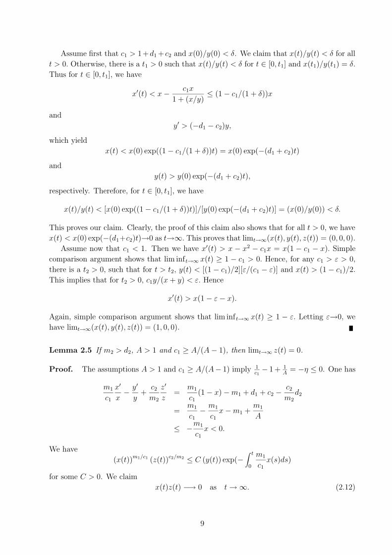
x(t)z(t) −→ 0 as t→∞. (2.12)

9

If not, then limt→∞ x(t) 6= 0. A similar argument for the proof of∫∞0 y(t)dt = +∞ in the

previous lemma yields that ∫ ∞

0x(t)dt = +∞

which implies (2.12), proving the claim.

Next, we claim that limt→∞ z(t) = 0. If not, then either limt→∞ z(t) exists with positive

limit or it does not exist. Assume first the former case. By (2.12), limt→∞ z(t) = z > 0

implies limt→∞ x(t) = 0. Using the same arguments in Lemma 2.4, we can show that

limt→∞ y(t) = 0 which implies limt→∞ z(t) = 0 and this is a contradiction. Assume now

the latter case, we have lim supt→∞ z(t) = z > 0. There exists tn ↑ ∞, z′(tn) = 0 and

z(tn)→ z as n→∞. We thus have

0 = z′(tn) = z(tn)

[m2y(tn)

y(tn) + z(tn)− d2

]

and

y(tn)→ y =d2z

m2 − d2

> 0

From (2.12), we have x(tn) → 0 as n → ∞. Hence P ≡ (0, y, z) ∈ Ω, the ω-limit set of

the trajectory (x(t), y(t), z(t)) : t ≥ 0. By the invariance of ω-limit set, it follows that

the backward trajectory of P is contained in Ω. We claim that the backward trajectory

(x(t), y(t), z(t)) : t ≤ 0 through P is unbounded. Obviously x(t) ≡ 0. Let τ = −t, then

dy

dτ= d1y +

c2yz

y + z≥ d1y

and

y(τ) ≥ y(0)ed1τ −→∞ as τ → +∞

This contradicts to the boundedness of the solution.

Combining Lemma 2.3, 2.4, 2.5 we have the following intuitive and sharp extinction

results of top predator.

Theorem 2.2 If the interior equilibrium Ec does not exist, then the top predator of model

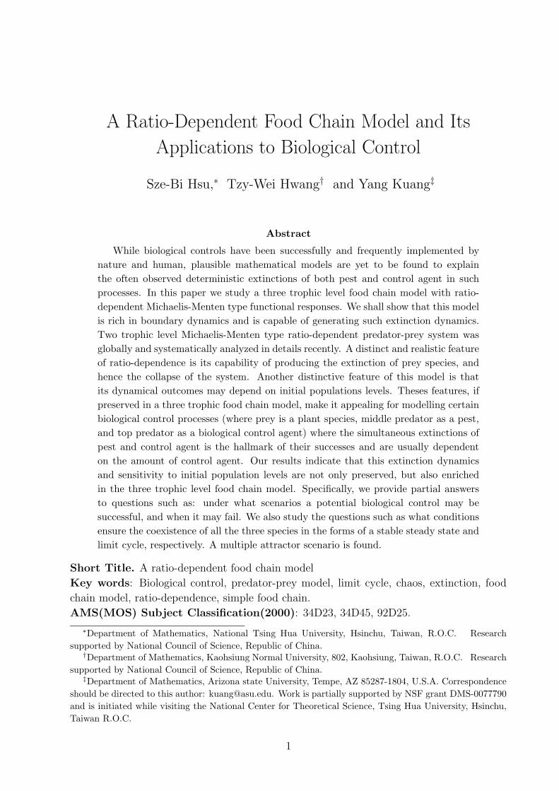
(2.1)-(2.3) will die out. Specifically, if one of the following three conditions holds, (i):

m2 ≤ d2; (ii): m2 > d2, 0 < A ≤ 1; (iii): m2 > d2, A > 1 and c1 ≥ A/(A − 1), then

limt→∞ z(t) = 0.

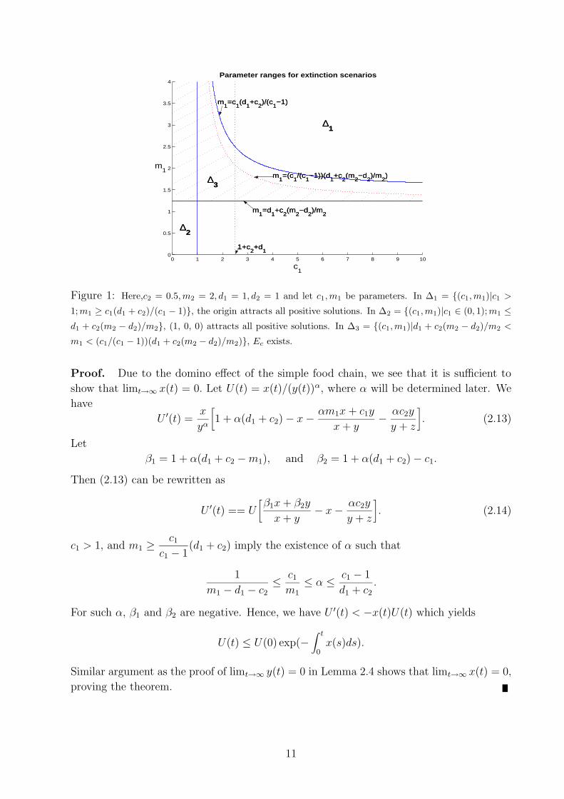
Let c2 = 0.5,m2 = 2, d1 = 1, d2 = 1 and let c1,m1 be parameters. Figure 1 illustrate the

parameter ranges for various extinction scenarios.

Our next theorem gives conditions for the origin as a global attractor for system (2.1)-

(2.3). Naturally, Ec does not exist in such scenario.

Theorem 2.3 If c1 > 1, and m1 ≥c1

c1 − 1(d1 + c2), then the origin is globally attractive.

That is, limt→∞(x(t), y(t), z(t)) = (0, 0, 0).

10

0 1 2 3 4 5 6 7 8 9 100

0.5

1

1.5

2

2.5

3

3.5

4

c1

m1

Parameter ranges for extinction scenarios

m1=d

1+c

2(m

2−d

2)/m

2

1+c2+d

1

m1=(c

1/(c

1−1))(d

1+c

2(m

2−d

2)/m

2)

m1=c

1(d

1+c

2)/(c

1−1)

∆1

∆3

∆2

m1=d

1+c

2(m

2−d

2)/m

2

1+c2+d

1

m1=(c

1/(c

1−1))(d

1+c

2(m

2−d

2)/m

2)

m1=c

1(d

1+c

2)/(c

1−1)

∆1

∆3

∆2

Figure 1: Here,c2 = 0.5,m2 = 2, d1 = 1, d2 = 1 and let c1,m1 be parameters. In ∆1 = (c1,m1)|c1 >

1;m1 ≥ c1(d1 + c2)/(c1 − 1), the origin attracts all positive solutions. In ∆2 = (c1,m1)|c1 ∈ (0, 1);m1 ≤

d1 + c2(m2 − d2)/m2, (1, 0, 0) attracts all positive solutions. In ∆3 = (c1,m1)|d1 + c2(m2 − d2)/m2 <

m1 < (c1/(c1 − 1))(d1 + c2(m2 − d2)/m2), Ec exists.

Proof. Due to the domino effect of the simple food chain, we see that it is sufficient to

show that limt→∞ x(t) = 0. Let U(t) = x(t)/(y(t))α, where α will be determined later. We

have

U ′(t) =x

yα

[1 + α(d1 + c2)− x−

αm1x+ c1y

x+ y−

αc2y

y + z

]. (2.13)

Let

β1 = 1 + α(d1 + c2 −m1), and β2 = 1 + α(d1 + c2)− c1.

Then (2.13) can be rewritten as

U ′(t) == U[β1x+ β2y

x+ y− x−

αc2y

y + z

]. (2.14)

c1 > 1, and m1 ≥c1

c1 − 1(d1 + c2) imply the existence of α such that

1

m1 − d1 − c2

≤c1

m1

≤ α ≤c1 − 1

d1 + c2

.

For such α, β1 and β2 are negative. Hence, we have U ′(t) < −x(t)U(t) which yields

U(t) ≤ U(0) exp(−∫ t

0x(s)ds).

Similar argument as the proof of limt→∞ y(t) = 0 in Lemma 2.4 shows that limt→∞ x(t) = 0,

proving the theorem.

11

3 Stability of Ec

In this section, we assume that Ec exists and study its local stability. This will yield some

analytic (explicit) and computational (implicit) conditions for both stable and oscillatory

coexistence of all three species.

The variational matrix of (2.1)-(2.3) at Ec is given by

M =

m11 m12 0

m21 m22 m23

0 m32 m33

(x,y,z)=(xc,yc,zc)

where

m11 = xc

[−1 +

c1yc(xc + yc)2

], (3.1)

m22 = yc

[−

m1xc

(xc + yc)2+

c2zc(zc + yc)2

], (3.2)

m33 = −m2yczc(yc + zc)2

. (3.3)

m12 = −c1x

2c

(xc + yc)2, m21 =

m1y2c

(xc + yc)2, m23 = −

c2y2c

(yc + zc)2, m32 =

m2z2c

(yc + zc)2.

The characteristic polynomial of M is

f(λ) = det(M − λI)

= (m11 − λ)(m22 − λ)(m33 − λ)−m12m21(m33 − λ)

−m23m32(m11 − λ).

Then the roots λ of f(λ) = 0 satisfy

λ3 + A1λ2 + A2λ+ A3 = 0,

where

A1 = −m11 −m22 −m33,

A2 = m22m33 +m11m22 +m11m33 −m12m21 −m23m32,

A3 = m12m21m33 +m11m23m32 −m11m22m33.

Straightforward computation shows that

A3 = detM = m1m2x2cy

2czc/[(yc + zc)(xc + yc)]

2 > 0.

From Roth-Hurwitz criterion, Ec is local asymptotically stable if and only if A1 > 0, A2 > 0,

A3 > 0 and A1A2 > A3.

In the following proposition, a sufficient condition is given for the local stability of Ec.

Proposition 3.1 If m11 < 0 and m22 < 0 then Ec is locally asymptotically stable.

12

Proof. From the signs of those defined mij, i, j = 1, 2, 3, it is easy to verify A1 > 0, A2 > 0

and A3 > 0. Expand A1A2 and calculate A1A2 − A3, then

A1A2 − A3 = −(m11)2m22 − (m11)

2m33 +m11m12m21 − (m22)2m33

−m11(m22)2 − 2m11m22m33 +m22m12m21 +m23m32m22

−m22(m33)2 −m11(m33)

2 +m23m32m33 > 0.

Hence Ec is local asymptotically stable.

We can express the conditions m11 < 0, m22 < 0 in terms of c1, c2. From (3.1), (2.4),

(2.7), (2.9), we have

m11 = xc

(−1 +

c1(A− 1)xc

A2x2c

)< 0 (3.4)

if and only if c1(A − 1) < A2xc = A (1 + (1− c1)(A− 1)) . Clearly, 0 < c1 ≤ 1 implies

m11 < 0. If c1 > 1, then m11 < 0 if and only if 1 < A <√c1/(c1 − 1).

From (3.2), (2.4), (2.7), (2.8), (2.9), we have

m22 < 0 ⇔c2zc

(zc + yc)2<

m1xc

(xc + yc)2

⇔ c2(m2/d2)− 1

(m2/d2)2<

m1(A− 1)

A2= m1

(1

A−1

A2

)

=

(c2

m2 − d2

m2

+ d1

)−1

m1

(c2

m2 − d2

m2

+ d1

)2

⇔ 0 < g(c2)

where

g(c2) = −1

m1

(c2

m2 − d2

m2

+ d1

)2

+ c2

(m2 − d2

m2

)+ d1

−c2(m2/d2)− 1

(m2/d2)2

Since g(0) > 0 and g(

m1−d1

(m2−d2)/m2

)< 0, there exist c∗2 > 0 such that g(c∗2) = 0.

Then

0 < c2 < c∗2 ⇔ m22 < 0

To discuss the instability of Ec we consider the possibility of choosing c1, c2 satisfying

A1 < 0. By (3.1)-(3.3), we have

A1 = I1 + I2

where

I1 = xc + (m1 − c1)(A− 1)

A2,

and

I2 = (m2 − c2)(m2/d2)− 1

(m2/d2)2.

13

0 5 10 15 20 250

0.2

0.4

0.6

0.8

1

c1

c2

Parameter range for the stability of Ec given by Proposition 3.1

A=1

A=c1/(c

1−1)

A=[c1/(c

1−1)]1/2

R is the stability region of Ec given

by m11

<0 and m22

<0R

1

c2=c

2*

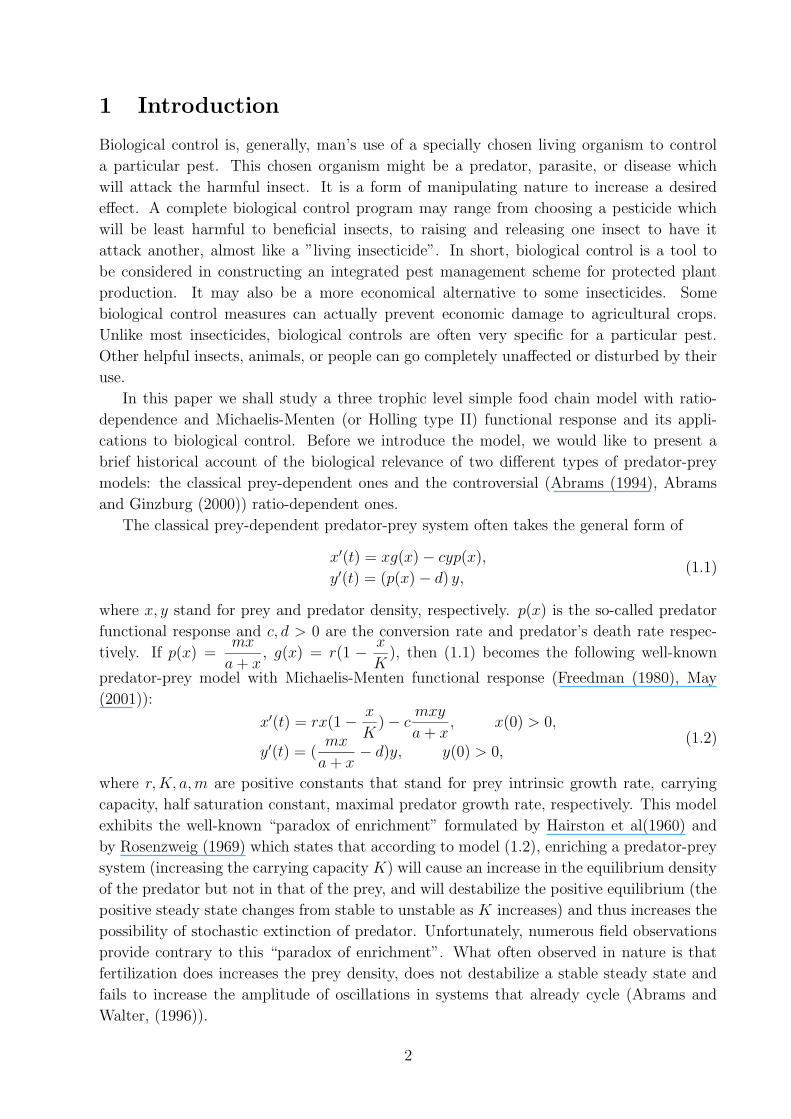
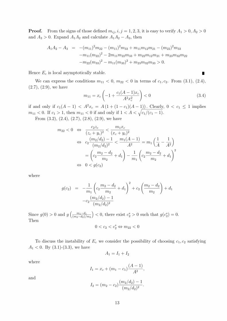
Figure 2: The parameter region for the the asymptotical stability of Ec given by Proposition 3.1, when

m1 = 1.5,m2 = 2, d1 = 1, d2 = 1. The region, denoted by R, is bounded by the two axes and the two curves

defined by c2 = c∗2 and A = (c1/(c1 − 1))1/2.

Observe that A = 1 if and only if c2 = m2(m1 − d1)/(m2 − d2). Hence we assume

m2 < m2(m1 − d1)/(m2 − d2), i.e. m2 − d2 < m1 − d1, (3.5)

and consider the case

m2 < c2 <m2(m1 − d1)

m2 − d2

then it follows that I2 < 0.

Notice that

I1 =1

A(1 + (1− c1)(A− 1)) + (m1 − c1)

A− 1

A2.

If A ≈ 1 then c2 ≈ m2(m1 − d1)/(m2 − d2), I1 ≈ 1 and

I2 ≈ (m2 −m2(m1 − d1)/(m2 − d2))((m2/d2)− 1)

(m2/d2)2

= (d2/m2)[(m2 − d2)− (m1 − d1)] < 0.

If we choose mi, di, i = 1, 2 such that

1 + [(m2 − d2)− (m1 − d1)] d2/m2 < 0,

or

m2/d2 < (m1 − d1)− (m2 − d2), (3.6)

then A1 < 0 for c2 near m2(m1 − d1)/(m2 − d2). Thus we have the following proposition.

Proposition 3.2 Let (3.5), (3.6) hold. Then Ec is unstable for m2 < c2 < m2(m1 −

d1)/(m2 − d2) and c2 is near m2(m1 − d1)/(m2 − d2).

14

0 2 4 6 8 10 120

2

4

6

8

10

12

14

16

18

20

c1

c2

Parameter range for the asymptotic stability of Ec

A=18

A=c1/(c

1−1)

A1A

2=A

3

A1A

2=A

3

A1=0

A=[c1/(c

1−1)]1/2

R2 is the asymptotic stability region of E

c

R2

R1

R3

1

c2=c

2*

R1

R1

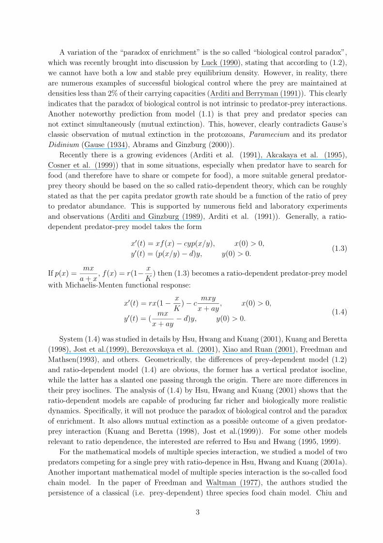
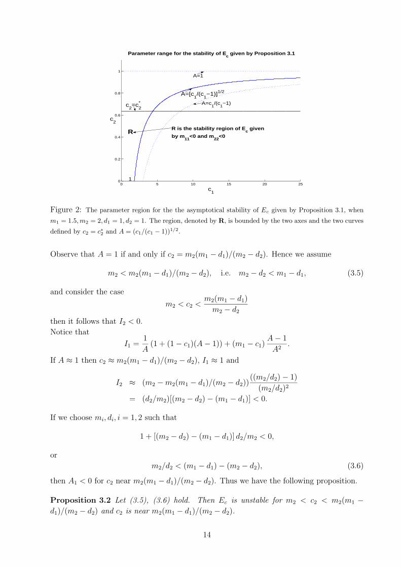
Figure 3: The parameter region for the the asymptotical stability of Ec, when m1 = 10,m2 = 2, d1 =

1, d2 = 1. The dot line filled region, denoted by R2, is bounded by the two axes and the two curves defined

by A = c1/(c1 − 1) and A1A2 = A3. A1 = 0 divides the figure into two parts, on the top and right side of

it, A1 < 0. So, even though A1A2 > A3 on the top of the existence region of Ec, Ec remains unstable.

There are two possible ways for Ec to change from stable to unstable: 1) at least one of

its eigenvalues change from negative to positive, and hence at the transition stage, at least

one of the eigenvalue assumes the value zero; 2) the real part of a pair of complex-conjugates

eigenvalues changes sign. Since when Ec exist, we always have detM = −λ1λ2λ3 > 0, we see

only the second way is actually taken. In Figure 3, we choose m1 = 10,m2 = 2, d1 = d2 = 1

and we plot the regions R1,R2,R3 in the c1 − c2 parameter plane where the equilibrium

Ec does not exist in R1; in region R2, Ec is local asymptotically stable with one negative

eigenvalue, two complex-conjugates with negative real parts; in region R3, Ec is a saddle

point with one negative eigenvalue and two complex-conjugates with positive real parts.

Clearly, Hopf bifurcation occurs if the parameters c1, c2 cross the boundary of R2 and R3,

∂R2 ∩ ∂R3.

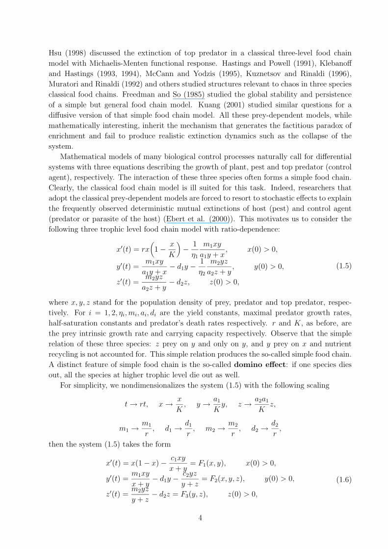
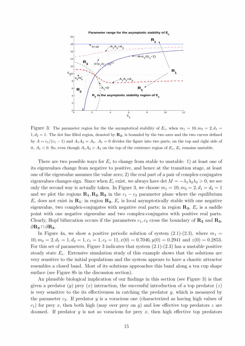
In Figure 4a, we show a positive periodic solution of system (2.1)-(2.3), where m1 =

10,m2 = 2, d1 = 1, d2 = 1, c1 = 1, c2 = 11, x(0) = 0.7046, y(0) = 0.2941 and z(0) = 0.2853.

For this set of parameters, Figure 3 indicates that system (2.1)-(2.3) has a unstable positive

steady state Ec. Extensive simulation study of this example shows that the solutions are

very sensitive to the initial populations and the system appears to have a chaotic attractor

resembles a closed band. Most of its solutions approaches this band along a tea cup shape

surface (see Figure 8b in the discussion section).

An plausible biological implication of our findings in this section (see Figure 3) is that

given a predator (y) prey (x) interaction, the successful introduction of a top predator (z)

is very sensitive to the its effectiveness in catching the predator y, which is measured by

the parameter c2. If predator y is a voracious one (characterized as having high values of

c1) for prey x, then both high (may over prey on y) and low effective top predators z are

doomed. If predator y is not so voracious for prey x, then high effective top predators

15

0.4

0.6

0.8

0.20.40.60.80.25

0.3

0.35

0.4

0.45

x

Figure 4a: A periodic solution

y

z

0 20 40 60 80 1000.2

0.4

0.6

0.8

Figure 4b: The periodic solution in t

t

x, y,

z

xy z

0 10 20 300

0.5

1

1.5

2

2.5

3Figure 4c

t

x, y,

z

xy z

0 10 20 30 400

0.5

1

1.5

2Figure 4d

t

x, y

xy

0.4

0.6

0.8

0.20.40.60.80.25

0.3

0.35

0.4

0.45

x

Figure 4a: A periodic solution

y

z

0 20 40 60 80 1000.2

0.4

0.6

0.8

Figure 4b: The periodic solution in t

t

x, y,

z

xyz

0 10 20 300

0.5

1

1.5

2

2.5

3Figure 4c

t

x, y,

z

xyz

0 10 20 30 400

0.5

1

1.5

2Figure 4d

t

x, y

xy

Figure 4: Figure 4a depicts a positive periodic solution of system (2.1)-(2.3), where m1 = 10,m2 = 2, d1 =

1, d2 = 1, c1 = 1, c2 = 11, x(0) = 0.7046, y(0) = 0.2941 and z(0) = 0.2853. Figure 4b depicts the time course

of this periodic solution. When we reduce c2 from 11 to 10, Ec becomes asymptotically stable. Figure 4c

depicts the time course of a solution tending to Ec. Figure 4d shows that without top predator, species x

and y coexist in the form of a stable steady state.

z are doomed while low and medium effective ones may endure. Moreover, low effective

top predators likely coexist with species y and thus x in the form of stable equilibria, while

medium effective top predators may generate population fluctuations in all the three species.

The implications of this section on biological control is somewhat subtle, we leave this

to the discussion section.

4 Sensitivity to Initial Conditions

It is well known that prey-dependent simple food chain models can generate chaotic dynam-

ics (Hastings and Powell (1991), Klebanoff and Hastings (1993, 1994), McCann and Yodzis

(1995), Kuznetsov and Rinaldi (1996)), which indicates that for some parameters, solutions

can be very sensitive to initial populations. We shall see that the ratio-dependent simple

food chain model (2.1)-(2.3) is also capable of generating this sensitive dynamics.

Theorem 2.2 implies that no complex dynamics is possible for system (2.1)-(2.3) if it

has no positive steady state Ec. Hence, in this section, we do not assume that the

interior equilibrium Ec = (xc, yc, zc) does not exists. In the xyz space, in addition to the

possible Ec, there maybe equilibria (0, 0, 0), (1, 0, 0), (x∗, y∗, 0). From the equation (2.3),

the equilibrium (x∗, y∗, 0) or the periodic orbit Γ in xy plane (if Γ exists where

Γ = (x∗(t), y∗(t), 0) : 0 ≤ t ≤ T, T is the period) is unstable in z-direction (when z(0)

is small and (x(0), y(0), z(0)) is near to the steady state (x∗, y∗, 0) or Γ = (x∗(t), y∗(t), 0) :

16

0 ≤ t ≤ T, we have ln(z(T )/z(0)) ≈ exp((m2 − d2)T ) > 1). Hence we only need to

discuss the possibilities of trajectories tending to (0, 0, 0) or (1, 0, 0). First we consider the

conditions for the existence of trajectories tending to (0, 0, 0). To this end, we introduce

u = x/y and v = y/z and the change of variables (x, y, z)→(u, y, v). Then (2.1)-(2.3) is

converted into following system:

u′ =u

1 + u(Au+B)− u2y +

c2u

1 + v, u(0) > 0, (4.1)

y′ =(

m1u

1 + u− d1

)y −

c2y

1 + v, y(0) > 0, (4.2)

v′ =[(

m1u

1 + u− d1

)−

c2

v + 1−(

m2v

1 + v− d2

)]v, v(0) > 0, (4.3)

where

A = 1− (m1 − d1), B = 1− c1 + d1. (4.4)

The system (4.1)-(4.3) has the following equilibria of the form:

E00 = (0, 0, 0),

E01 = (0, 0, v), v > 0,

E10 = (θ∗1, 0, 0), θ∗1 > 0,

E11 = (θ∗2, 0, v), θ∗2 > 0, v > 0.

From the domino effect of simple food chain, it is easy to see that

1. (u(t), y(t), v(t))→ E00 as t→∞ if and only if (x(t), y(t), z(t))→ (0, 0, 0) and x(t)→ 0

faster than y(t)→ 0, y(t)→ 0 faster than z(t)→ 0.

2. (u(t), y(t), v(t)) → E01 if and only if (x(t), y(t), z(t)) → (0, 0, 0) and x(t) → 0 faster

than y(t)→ 0, z(t)→ 0 at finite rate as y(t)→ 0.

3. (u(t), y(t), v(t)) → E10 if and only if (x(t), y(t), z(t)) → (0, 0, 0) and y(t) → 0 faster

than z(t), x(t)→ 0 at finite rate as y(t)→ 0.

4. (u(t), y(t), v(t))→ E11 if and only if y(t)→ 0 and x(t)→ 0, z(t)→ 0 at finite rate as

y(t)→ 0.

The equilibrium E00 = (0, 0, 0) of (4.1)-(4.3) always exists. The variational matrix at

E00 is

J(E00) =

B + c2 0 0

0 −d2 − c2 0

0 0 −d1 − c2 + d2

.

From (4.4), E00 is asymptotically stable if and only if

1 + d1 + c2 < c1 and d2 − d1 < c2. (4.5)

For the existence of the equilibrium E01 = (0, 0, v), from equation of (4.3), v > 0 satisfies

d2 − d1 =m2v + c2

v + 1. (4.6)

17

Hence

E01 exists if and only if d2 − d1 > 0 and d2 − d1 is between m2 and c2. (4.7)

The variational matrix at E01 is

J(E01) =

B + c21+v

0 0

0 −d1 −c2

1+v0

m1v 0 v[

c2(v+1)2

− m2

(1+v)2

]

.

E01 is asymptotically stable if and only if

1 + d1 +c2

1 + v< c1 and c2 < m2.

This together with (3.13) imply that E01 exists and is asymptotically stable if and only if

1 + d1 +c2(m2 + d1 − d2)

m2 − c2

< c1 and c2 < d2 − d1 < m2. (4.8)

For the existence of the equilibrium E10 = (θ∗1, 0, 0), from equation (4.1), θ

∗1 satisfies

θ∗1 =−(B + c2)

A+ c2

. (4.9)

Hence

E10 exists if and only if (B + c2)(A+ c2) < 0. (4.10)

The variational matrix at E10 is

J(E10) =

(A−B)u(1+u)2

−u2 −c2u

0 m1u1+u

− d1 − c2 0

0 0 m1u1+u

− d1 − c2 + d2

u=θ∗1

.

E10 is asymptotically stable if and only if

A < B ,m1θ

∗1

1 + θ∗1+ d2 < d1 + c2.

This together with (4.4) and (4.10) imply that E10 exists and is asymptotically stable if and

only if

m1 > 1 + d1 + c2 > c1 , m1(1 + d2 − c1) < c1(d2 − c2 − d1). (4.11)

For example, d1 = 0.6, d2 = 0.2,m1 = 3,m2 = 1, c1 = 2, c2 = 0.6 satisfy the above condition.

For the existence of the equilibrium E11 = (θ∗2, 0, v), (4.1) and (4.3) imply that θ

∗2 and v

satisfyB + Aθ∗21 + θ∗2

+c2

1 + v= 0,

andm1θ

∗2

1 + θ∗2− d1 −

c2

1 + v−(

m2v

v + 1− d2

)= 0.

The stability analysis of E11 is rather complicated and we forgo it here.

Our next result provides another set of conditions for the origin to be a local attractor.

Notice that the result is an improvement of the first part of Theorem 2.1 when m1 <

c1(d1 + c2)/(c1 − 1). In addition, the conditions do not exclude the existence of Ec.

18

Proposition 4.1 Assume that c1 > 1+d1+c2 and m1 < c1(d1+c2)/(c1−1). If, in addition,

x(0)

y(0)≤

c1 − (1 + d1 + c2)

1 + d1 + c2 −m1

≡ u0,

then limt→∞(x(t), y(t), z(t)) = (0, 0, 0).

Proof. Due to the domino effect of the simple food chain, we need only to show that

limt→∞ x(t) = 0. Let u(t) = x(t)/(y(t). We have

u′(t) = u[(1 + d1 + c2 −m1)

u− u0

1 + u− x−

c2y

y + z

].

Clearly, for t > 0, u(t) ≤ u0 if u(0) ≤ u0. Hence

u(t) ≤ u(0) exp(−∫ t

0x(s)ds).

The rest follows from the argument of Theorem 2.3 that yields limt→∞ x(t) = 0.

Next we consider the conditions for the existence of trajectories of (2.1)-(2.3) tending to

E1 = (1, 0, 0) as t→∞.

Proposition 4.2 Assume that m2 > d2 and m1 < min1+d1, d1+ c2−d2. Then there are

solutions of (2.1)-(2.3) tending to E1 = (1, 0, 0) as t→∞.

Proof. Observe that (4.1)-(4.3) can be rewritten as

u′ = u2[Au+B

u(1 + u)+

c2

u(1 + v)− y

]= u2[K(u, v)− y] ≡ G1(u, y, v), u(0) > 0,

y′ = y[−m1

1 + u+

l1v + l21 + v

]≡ G2(u, y, v), y(0) > 0,

v′ = v[−m1

1 + u+

q1v + q2

1 + v

]≡ G3(u, y, v), v(0) > 0,

where A = 1−m1+ d1, B = 1− c1+ d1, l1 = m1− d1, l2 = m1− d1− c2, q1 = m1− d1+ d2−

m2, q2 = m1 − d1 + d2 − c2.

Clearly, A > 0 > q2 > l2. Hence there is a v0 > 0 such that G2(u, y, v) < 0 and

G3(u, y, v) < 0 for all (u, y, v) ∈ [0,∞)× [0,∞)× [0, v0]. Let u0 = max−B/A, 0 ≥ 0 and

Ω ≡ (u, y, v) ∈ R3+|u ∈ [u0,∞), v ∈ [0, v0], y ∈ [0, K(u0, v0)].

Then Ω is positively invariant. Since there is no equilibrium in Ω, the monotonicity of the

components of the solution in Ω implies that limt→∞(u(t), y(t), v(t)) = (+∞, 0, 0). Therefore,

if x(0) ≥ u0y(0), y(0) ≤ v0z(0) and y(0) < K(u0, v0), then limt→∞ x(t)/y(t) = +∞. This

shows that for any ε > 0, there is a Tε > 0 such that for t ≥ Tε, we have

c1y(t)

x(t) + y(t)=

c1

1 + x(t)/y(t)< ε.

From (2.1), we have x′(t) > x(t)(1− ε− x(t)) for all t ≥ Tε. Standard argument shows that

limt→∞ x(t) = 1, proving the proposition.

19

To obtain additional results on the conditions for the existence of trajectories of (2.1)-

(2.3) tending to E1 = (1, 0, 0) as t → ∞, we let v = y/z and consider the transformation

(x, y, z)→ (x, y, v). Then (2.1)-(2.3) is converted into the following system:

x′ = x(1− x)− c1xyx+y

, x(0) > 0,

y′ =(m1xx+y

− d1 −c2v+1

)y, y(0) > 0,

v′ = v[(

m1xx+y

− d1 −c2v+1

)−(m2vv+1

− d2

)], v(0) > 0.

(4.12)

The system (4.12) has the following equilibria of the form:

E100 = (1, 0, 0),

E101 = (1, 0, v), v > 0.

E100 always exists. From the third equation of (4.12), v satisfies

m1 − d1 + d2 =m2v + c2

v + 1. (4.13)

Hence E101 exists if and only if m1 − d1 + d2 is between m2 and c2.

The variational matrix of (4.12) at E100 is

J(E100) =

−1 −c1 0

0 m1 − d1 − c2 0

0 0 m1 − d1 − c2 + d2

.

Hence E100 is asymptotically stable if and only if

m1 + d2 < d1 + c2. (4.14)

The variational matrix of (4.12) at E101 is

J(E101) =

−1 −c1 0

0 m1 − d1 − c2/(v + 1) 0

0 −m1v v(c2 −m2)/(v + 1)2

.

Hence E101 is asymptotically stable if and only if

m1 < d1 +c2

v + 1and c2 < m2. (4.15)

From (4.13), (4.15) can be rewritten as

(m2 − d2)c2 > (m1 − d1)m2 and c2 < m2. (4.16)

We summarize some of the key findings of this section into the following theorem.

Theorem 4.1 If at least one of the following four condition hold

1): 1 + d1 + c2 < c1 and d2 − d1 < c2;

2): 1 + d1 +c2(m2+d1−d2)

m2−c2< c1 and c2 < d2 − d1 < m2;

3): m1 > 1 + d1 + c2 > c1 , m1(1 + d2 − c1) < c1(d2 − c2 − d1);

20

0

0.5

1

1.5 0

0.05

0.1

0

0.1

0.2

0.3

0.4

0.5

y

q

Figure 5a

p

x

z

0 0.2 0.4 0.6 0.8 10

0.1

0.2

0.3

0.4

0.5

0.6Figure 5b

pxy

qxy

x

y

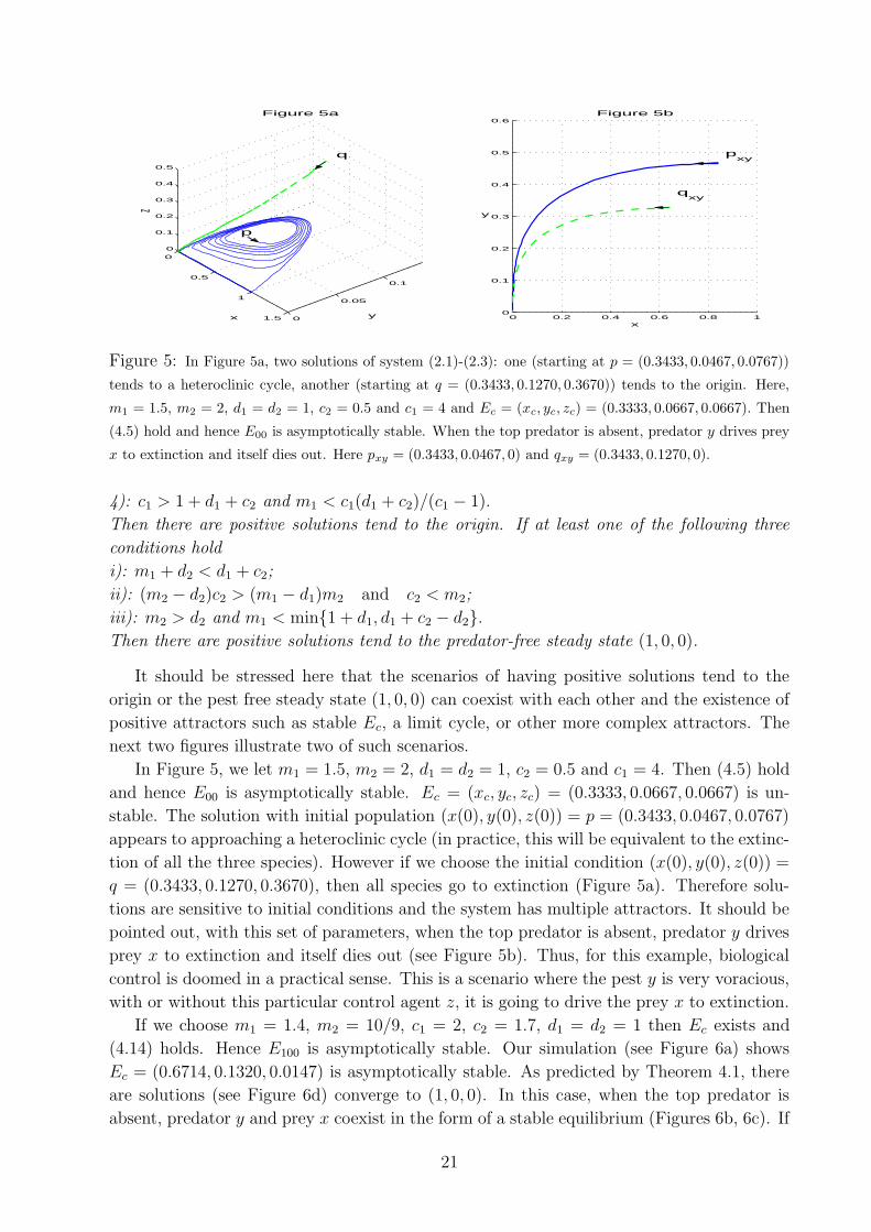
Figure 5: In Figure 5a, two solutions of system (2.1)-(2.3): one (starting at p = (0.3433, 0.0467, 0.0767))

tends to a heteroclinic cycle, another (starting at q = (0.3433, 0.1270, 0.3670)) tends to the origin. Here,

m1 = 1.5, m2 = 2, d1 = d2 = 1, c2 = 0.5 and c1 = 4 and Ec = (xc, yc, zc) = (0.3333, 0.0667, 0.0667). Then

(4.5) hold and hence E00 is asymptotically stable. When the top predator is absent, predator y drives prey

x to extinction and itself dies out. Here pxy = (0.3433, 0.0467, 0) and qxy = (0.3433, 0.1270, 0).

4): c1 > 1 + d1 + c2 and m1 < c1(d1 + c2)/(c1 − 1).

Then there are positive solutions tend to the origin. If at least one of the following three

conditions hold

i): m1 + d2 < d1 + c2;

ii): (m2 − d2)c2 > (m1 − d1)m2 and c2 < m2;

iii): m2 > d2 and m1 < min1 + d1, d1 + c2 − d2.

Then there are positive solutions tend to the predator-free steady state (1, 0, 0).

It should be stressed here that the scenarios of having positive solutions tend to the

origin or the pest free steady state (1, 0, 0) can coexist with each other and the existence of

positive attractors such as stable Ec, a limit cycle, or other more complex attractors. The

next two figures illustrate two of such scenarios.

In Figure 5, we let m1 = 1.5, m2 = 2, d1 = d2 = 1, c2 = 0.5 and c1 = 4. Then (4.5) hold

and hence E00 is asymptotically stable. Ec = (xc, yc, zc) = (0.3333, 0.0667, 0.0667) is un-

stable. The solution with initial population (x(0), y(0), z(0)) = p = (0.3433, 0.0467, 0.0767)

appears to approaching a heteroclinic cycle (in practice, this will be equivalent to the extinc-

tion of all the three species). However if we choose the initial condition (x(0), y(0), z(0)) =

q = (0.3433, 0.1270, 0.3670), then all species go to extinction (Figure 5a). Therefore solu-

tions are sensitive to initial conditions and the system has multiple attractors. It should be

pointed out, with this set of parameters, when the top predator is absent, predator y drives

prey x to extinction and itself dies out (see Figure 5b). Thus, for this example, biological

control is doomed in a practical sense. This is a scenario where the pest y is very voracious,

with or without this particular control agent z, it is going to drive the prey x to extinction.

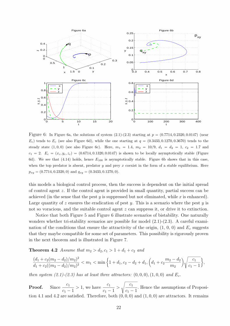
If we choose m1 = 1.4, m2 = 10/9, c1 = 2, c2 = 1.7, d1 = d2 = 1 then Ec exists and

(4.14) holds. Hence E100 is asymptotically stable. Our simulation (see Figure 6a) shows

Ec = (0.6714, 0.1320, 0.0147) is asymptotically stable. As predicted by Theorem 4.1, there

are solutions (see Figure 6d) converge to (1, 0, 0). In this case, when the top predator is

absent, predator y and prey x coexist in the form of a stable equilibrium (Figures 6b, 6c). If

21

0

0.5

1

1.5 0

0.1

0.2

0.3

0

0.2

0.4

y

p

Figure 6a

q

x

z

0.3 0.4 0.5 0.6 0.7 0.80

0.05

0.1

0.15

0.2

0.25Figure 6b

pxy

qxy

x

y

0 5 10 15 200

0.2

0.4

0.6

0.8

1Figure 6c

t

x, y,

z

xyz

0 100 200 300 4000

0.2

0.4

0.6

0.8Figure 6d

tx,

y, z

xyz

0

0.5

1

1.5 0

0.1

0.2

0.3

0

0.2

0.4

y

p

Figure 6a

q

x

z

0.3 0.4 0.5 0.6 0.7 0.80

0.05

0.1

0.15

0.2

0.25Figure 6b

pxy

qxy

x

y

0 5 10 15 200

0.2

0.4

0.6

0.8

1Figure 6c

t

x, y,

z

xyz

0 100 200 300 4000

0.2

0.4

0.6

0.8Figure 6d

tx,

y, z

xyz

Figure 6: In Figure 6a, the solutions of system (2.1)-(2.3) starting at p = (0.7714, 0.2320, 0.0147) (near

Ec) tends to Ec (see also Figure 6d), while the one starting at q = (0.3433, 0.1270, 0.3670) tends to the

steady state (1, 0, 0) (see also Figure 6c). Here, m1 = 1.4, m2 = 10/9, d1 = d2 = 1, c2 = 1.7 and

c1 = 2. Ec = (xc, yc, zc) = (0.6714, 0.1320, 0.0147) is shown to be locally asymptotically stable (Figure

6d). We see that (4.14) holds, hence E100 is asymptotically stable. Figure 6b shows that in this case,

when the top predator is absent, predator y and prey x coexist in the form of a stable equilibrium. Here

pxy = (0.7714, 0.2320, 0) and qxy = (0.3433, 0.1270, 0).

this models a biological control process, then the success is dependent on the initial spread

of control agent z. If the control agent is provided in small quantity, partial success can be

achieved (in the sense that the pest y is suppressed but not eliminated, while x is enhanced).

Large quantity of z ensures the eradication of pest y. This is a scenario where the pest y is

not so voracious, and the suitable control agent z can suppress it, or drive it to extinction.

Notice that both Figure 5 and Figure 6 illustrate scenarios of bistability. One naturally

wonders whether tri-stability scenarios are possible for model (2.1)-(2.3). A careful exami-

nation of the conditions that ensure the attractivity of the origin, (1, 0, 0) and Ec suggests

that they maybe compatible for some set of parameters. This possibility is rigorously proven

in the next theorem and is illustrated in Figure 7.

Theorem 4.2 Assume that m2 > d2, c1 > 1 + d1 + c2 and

(d1 + c2(m2 − d2)/m2)2

d1 + c2((m2 − d2)/m2)2< m1 < min

1 + d1, c2 − d2 + d1,

(d1 + c2

m2 − d2

m2

)√c1

c1 − 1

,

then system (2.1)-(2.3) has at least three attractors: (0, 0, 0), (1, 0, 0) and Ec.

Proof. Sincec1

c1 − 1> 1, we have

c1

c1 − 1>

√c1

c1 − 1. Hence the assumptions of Proposi-

tion 4.1 and 4.2 are satisfied. Therefore, both (0, 0, 0) and (1, 0, 0) are attractors. It remains

22

00.5

1 0

0.02

0.04

0

0.1

0.2

y

p1

00.5

1 0

0.02

0.04

0

0.1

0.2

y

p1

x

Figure 7a

pc

p0

z

0 2 4 6 8 100

0.2

0.4

0.6

0.8

1

Figure 7b

t

x, y,

z

xyz

0 50 100 150 2000

0.2

0.4

0.6

0.8

1Figure 7c

t

x, y,

z

xyz

0 2 4 6 8 100

0.02

0.04

0.06

0.08

0.1Figure 7d

tx,

y, z

xyz

x

Figure 7a

pc

p0

z

0 2 4 6 8 100

0.2

0.4

0.6

0.8

1

0 50 100 150 2000

0.2

0.4

0.6

0.8

1

0 2 4 6 8 100

0.02

0.04

0.06

0.08

0.1

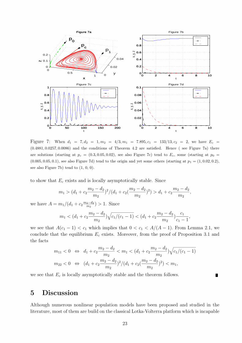
Figure 7: When d1 = 7, d2 = 1,m2 = 4/3,m1 = 7.895, c1 = 133/13, c2 = 2, we have Ec =

(0.4881, 0.0257, 0.0086) and the conditions of Theorem 4.2 are satisfied. Hence ( see Figure 7a) there

are solutions (starting at pc = (0.3, 0.05, 0.02), see also Figure 7c) tend to Ec, some (starting at p0 =

(0.005, 0.05, 0.1), see also Figure 7d) tend to the origin and yet some others (starting at p1 = (1, 0.02, 0.2),

see also Figure 7b) tend to (1, 0, 0).

to show that Ec exists and is locally asymptotically stable. Since

m1 > (d1 + c2m2 − d2

m2

)2/(d1 + c2(m2 − d2

m2

)2) > d1 + c2m2 − d2

m2

,

we have A = m1/(d1 + c2m2−d2

m2) > 1. Since

m1 < (d1 + c2m2 − d2

m2

)√c1/(c1 − 1) < (d1 + c2

m2 − d2

m2

)c1

c1 − 1,

we see that A(c1 − 1) < c1 which implies that 0 < c1 < A/(A − 1). From Lemma 2.1, we

conclude that the equilibrium Ec exists. Moreover, from the proof of Proposition 3.1 and

the facts

m11 < 0 ⇔ d1 + c2m2 − d2

m2

< m1 < (d1 + c2m2 − d2

m2

)√c1/(c1 − 1)

m22 < 0 ⇔ (d1 + c2m2 − d2

m2

)2/(d1 + c2(m2 − d2

m2

)2) < m1,

we see that Ec is locally asymptotically stable and the theorem follows.

5 Discussion

Although numerous nonlinear population models have been proposed and studied in the

literature, most of them are build on the classical Lotka-Volterra platform which is incapable

23

of describing both the vast biodiversity that we are part of and the massive extinction that

we are now confronting. This is likely due to the fact that conventional ecological studies are

often conducted in a small and controllable scale and thus enables the researchers to make

the implicit assumption that populations are quasi-stable or near a stable steady state.

Hence, most of the existing theoretical works on such mathematical models are centered

around stability issues of possible positive steady states (coexisting equilibria). In other

words, extinction dynamics is often overlooked or avoided. As a result, most models of

population interactions are incapable of producing extinctions at lower levels that typically

trigger the massive extinctions that we are witnessing today. In the context of biological

control, rich extinction dynamics of any plausible model is especially desirable.

A valid ratio-dependent model formulation usually requires that the habitat of the inter-

acting species is relatively small and free of refugees (Cosner et al. (1999)). The continual

fragmentation and shrinkage of habitats is often viewed as the main causes of massive ex-

tinctions of populations. Also, biological control is often successfully implemented in a

relatively small area. This makes ratio-dependent based population models relevant and

appealing due to their rich extinction dynamics. Our work on the ratio-dependent simple

food chain (2.1)-(2.3) suggests that ratio-dependence is a plausible mechanism that con-

tributes to both the massive extinctions of populations and the successful implementations

of biological controls.

Extensive simulation of model (2.1)-(2.3) confirms the notion that the introduction of a

natural enemy z for pest y helps the population level of prey x. This is illustrated by Figure

4. Without top predator, prey is severely depressed (Figure 4d). With a medium aggressive

(medium c2 values) top predator, species may coexist in a stable form with enhanced prey

and depressed pest population levels (see Figure 4c). A more voracious top predator may

slightly increase further the average prey level and decrease average pest level at the expense

of destabilizing such stable coexistence (see Figure 4b).

Our simulation work also shed light to the following interesting question: assume that

a voracious pest y (defined as any pest (predator) species that capable of driving its host

(prey) to extinction) invades a host x, can one introduce a suitable top predator to ensure

a meaningful (with some success) biological control? Figure 5 suggests the answer can be

positive. In such situations, it maybe necessary to introduce the control agent swiftly and

forcefully (see the solution starts at p) in order to slow down and or even stop the extinction

of x. A delayed action can mean total failure (see the solution starts at q).

Our extinction results suggest that biological control is possible under various scenarios.

However, in practice, we often want to reduce the pest y to an acceptable level in a finite time.

In order to accomplish that, we need to give a estimate as how much z shall be introduced

to control y. Clearly, theoretical findings are powerless for this particular practical concern.

Nevertheless, such an estimation work can be meaningfully conducted by some carefully

designed simulations of model (2.1)-(2.3).

A most startling finding of this paper is the discovery of a tri-stability scenario described

in Theorem 4.2. To the best of our knowledge, such sensitivity, although may very well exist

in other low dimensional (two or three dimensional autonomous ODE models) models, has

never been identified explicitly in the literature. Extensive simulation on the model (2.1)-

24

0.2 0.4 0.6 0.8 10

0.5

1

1.5

2

2.5

3

p

x

Figure 8a

q

y

0.20.40.60.81

0

1

2

3

0

0.5

1

x

Figure 8b

y

z0 100 200 300 400 500 600

0

0.5

1

1.5

2

2.5

3

t, Figure 8c

x, y,

z

xyz

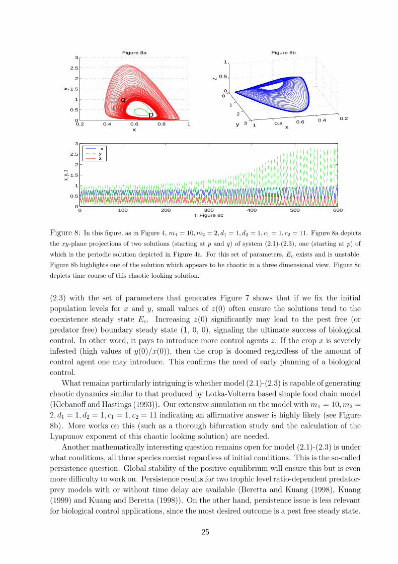
Figure 8: In this figure, as in Figure 4, m1 = 10,m2 = 2, d1 = 1, d2 = 1, c1 = 1, c2 = 11. Figure 8a depicts

the xy-plane projections of two solutions (starting at p and q) of system (2.1)-(2.3), one (starting at p) of

which is the periodic solution depicted in Figure 4a. For this set of parameters, Ec exists and is unstable.

Figure 8b highlights one of the solution which appears to be chaotic in a three dimensional view. Figure 8c

depicts time course of this chaotic looking solution.

(2.3) with the set of parameters that generates Figure 7 shows that if we fix the initial

population levels for x and y, small values of z(0) often ensure the solutions tend to the

coexistence steady state Ec. Increasing z(0) significantly may lead to the pest free (or

predator free) boundary steady state (1, 0, 0), signaling the ultimate success of biological

control. In other word, it pays to introduce more control agents z. If the crop x is severely

infested (high values of y(0)/x(0)), then the crop is doomed regardless of the amount of

control agent one may introduce. This confirms the need of early planning of a biological

control.

What remains particularly intriguing is whether model (2.1)-(2.3) is capable of generating

chaotic dynamics similar to that produced by Lotka-Volterra based simple food chain model

(Klebanoff and Hastings (1993)). Our extensive simulation on the model withm1 = 10,m2 =

2, d1 = 1, d2 = 1, c1 = 1, c2 = 11 indicating an affirmative answer is highly likely (see Figure

8b). More works on this (such as a thorough bifurcation study and the calculation of the

Lyapunov exponent of this chaotic looking solution) are needed.

Another mathematically interesting question remains open for model (2.1)-(2.3) is under

what conditions, all three species coexist regardless of initial conditions. This is the so-called

persistence question. Global stability of the positive equilibrium will ensure this but is even

more difficulty to work on. Persistence results for two trophic level ratio-dependent predator-

prey models with or without time delay are available (Beretta and Kuang (1998), Kuang

(1999) and Kuang and Beretta (1998)). On the other hand, persistence issue is less relevant

for biological control applications, since the most desired outcome is a pest free steady state.

25

Model (2.1)-(2.3) is most suitable when biological control agent is a natural predator

of the pest. Other models may also be plausible for this situation. For example, one may

use the classical prey-dependent functional response xy/(a1 + x) for pest and its numerical

response, while using ratio-dependent functional response yz/(y+a2z) for top predator and

its numerical response. This is particular suitable when pest is uniformly distributed and

slow moving. This mixed selection of functional response yields a model of the following

form

x′(t) = rx(1−

x

K

)−1

η1

m1xy

a1 + x, x(0) > 0,

y′(t) =m1xy

a1 + x− d1y −

1

η2

m2yz

a2z + y, y(0) > 0,

z′(t) =m2yz

a2z + y− d2z, z(0) > 0,

(5.1)

where the meanings of the parameters are self-evident. This model may also be capable of

admitting a pest free attractor. If parasite is chosen as the control agent, then quite differ-

ent model maybe called for. A plausible model may build a simple infection mechanism on

top of a typical predator-prey model with either prey-dependent or ratio-dependent (or the

more general predator-dependent ones) functional responses. The model can take various

forms depending on the specific choices of infection mechanisms and the predator functional

responses. Appropriately formulated, such models shall also be able to generate rich extinc-

tion dynamics. An example of such models with prey-dependent functional response may

take the form

x′(t) = rx(1−

x

K

)−

c1x(y + z)

a+ x, x(0) > 0,

y′(t) =m1x(y + fz)

a+ x− dy −

c2yz

y + z, y(0) > 0,

z′(t) =m2yz

y + z− (d+ α)z, z(0) > 0.

(5.2)

The infection mechanism is the same one adopted by Ebert et al. (2000) (but was erroneously

implemented in their model, causing the failure of generating deterministic extinction sce-

narios that needed to explain such phenomena in the fields, see Hwang and Kuang (2001)).

This mechanism can be used to model a microparasite transmission for a horizontally trans-

mitted parasite that reduces fecundity and survival of its host. In this case, the plausible

meanings of the parameters are again clear. It will be interesting to know if the naturally

occurring ratio-dependence (resulted from the infection mechanism) in the uninfected (y)

and the infected pest (z) equations will generate rich extinction dynamics that naturally

account for the various deterministic extinction scenarios observed in the fields.

26

References

[1] P. A. Abrams(1994): The fallacies of “ratio-dependent” predation, Ecology, 75, 1842-

1850.

[2] P. A. Abrams and C. J. Walters(1996): Invulnerable prey and the paradox of enrich-

ment, Ecology, 77, 1125-1133.

[3] P. A. Abrams and L. R. Ginzburg(2000): The nature of predation: prey dependent,

ratio-dependent or neither? Trends in Ecology and Evolution, 15, 337-341.

[4] H. R. Akcakaya, R. Arditi and L. R. Ginzburg(1995): Ratio-dependent prediction: an

abstraction that works, Ecology, 76, 995-1004.

[5] R. Arditi, A. A. Berryman(1991): The biological control paradox, Trends in Ecology

and Evolution 6, 32.

[6] R. Arditi and L. R. Ginzburg(1989): Coupling in predator-prey dynamics: ratio-

dependence, J. Theor. Biol., 139, 311-326.

[7] R. Arditi, L. R. Ginzburg and H. R. Akcakaya(1991): Variation in plankton densities

among lakes: a case for ratio-dependent models. American Natrualist 138, 1287-1296.

[8] E. Beretta and Y. Kuang(1998): Global analyses in some delayed ratio-dependent

predator-prey systems, Nonlinear Analysis, TMA., 32, 381-408.

[9] F. Berezovskaya, G. Karev and R. Arditi(2001): Parametric analysis of the ratio-

dependent predator-prey model, J. Math. Biol. 43, 221-246.

[10] A. A. Berryman(1992): The origins and evolution of predator-prey theory, Ecology

73, 1530-1535.

[11] A. A. Berryman, A. P. Gutierrez and R. Arditi(1995): Credible, realistic and useful

predator-prey models, Ecology, 76, 1980-1985.

[12] C. H. Chiu, S. B. Hsu(1998): Extinction of top predator in a three level food-chain

model, J. Math. Biol. 37, 372-380.

[13] C. Cosner, D. L. DeAngelis, J. S. Ault and D. B. Olson(1999): Effects of spatial

grouping on the functional response of predators, Theor. Pop. Biol., 56, 65-75.

[14] D. Ebert, M. Lipstich and K. L. Mangin(2000): The effect of parasites on host pop-

ulation density and extinction: experimental epidemiology with Daphnia and six mi-

croparasites, American Natrualist 156, 459-477.

[15] M. Fischer(2000): Species loss after habitat fragmentation, Trends in Ecology and

Evolution, 15, 396.

[16] H. I. Freedman(1980): Deterministic Mathematical Models in Population Ecology,

Marcel Dekker, New York.

27

[17] H. I. Freedman and R. M. Mathsen(1993): Persistence in predator-prey systems with

ratio-dependent predator-influence, Bull. Math. Biol., 55, 817-827.

[18] H. I. Freedman and J. W.-H. So(1985): Global stability and persistence of simple food

chains, Math. Biosci., 76, 69-86.

[19] H. I. Freedman and P. Waltman(1977): Mathematical analysis of some three-species

food-chain models, Math. Biosci. 33, 257-276.

[20] G. F. Gause(1934): The struggle for existence, Williams & Wilkins, Baltimore, Mary-

land, USA.

[21] N. G. Hairston, F. E. Smith and L. B. Slobodkin(1960): Community structure, popu-

lation control and competition, American Naturalist 94, 421-425.

[22] J. Hale(1980): Ordinary Differential Equations, Krieger Publ. Co., Malabar.

[23] G. W. Harrison(1995): Comparing predator-prey models to Luckinbill’s experiment

with Didinium and Paramecium, Ecology, 76, 357-374.

[24] A. Hastings and T. Powell(1991): Chaos in a three-species food chain, Ecology, 72,

896-903.

[25] S.-B. Hsu and T.-W. Hwang(1995): Global stability for a class of predator-prey sys-

tems, SIAM J. Appl. Math., 55, 763-783.

[26] S. B. Hsu, T. W. Hwang(1999): Hopf bifurcation for a predator-prey system of Holling

and Lesile type, Taiwanese J. Math., 3, 35-53.

[27] S. B. Hsu, T. W. Hwang and Y. Kuang(2001): Global Analysis of the Michaelis-Menten

type ratio-dependence predator-prey system, J. Math. Biol., 42, 489-506.

[28] S. B. Hsu, T. W. Hwang and Y. Kuang(2001a): Rich dynamics of a ratio-dependent

one prey two predator model, J. Math. Biol., to appear.

[29] T.-W. Hwang(1999): Uniquencess of limit cycle for Gause-type predator-prey systems,

J. Math. Anal. Appl. 238, 179-195.

[30] T. W. Hwang and Y. Kuang(2001): Extinction effect of parasites on host populations,

preprint.

[31] C. Jost, O. Arino and R. Arditi(1999): About deterministic extinction in ratio-

dependent predator-prey models, Bull. Math. Biol., 61, 19-32.

[32] A. Klebanoff and A. Hastings(1993): Chaos in three species food chains, J. Math.

Biol., 32, 427-451.

[33] A. Klebanoff and A. Hastings(1994): Chaos in one-predator, two-prey models: general

results from bifurcation theory, Math. Biosc., 122, 221-233

28

[34] Y. Kuang(1999): Rich dynamics of Gause-type ratio-dependent predator-prey system,

The Fields Institute Communications, 21, 325-337.

[35] Y. Kuang(2001): Global stability and persistence in diffusive food chains, (24 pages),

to appear in The ANZIAM journal (formerly the J. Austral. Math. Soc. B.), 43, part

II.

[36] Y. Kuang and E. Beretta(1998): Global qualitative analysis of a ratio-dependent

predator-prey system, J. Math. Biol., 36, 389–406.

[37] Yu. A. Kuznetsov and S. Rinaldi(1996): Remarks on food chain dynamics, Math.

Biosci., 134, 1-33.

[38] R. F. Luck(1990): Evaluation of natural enemies for biological control: a behavior

approach, Trends in Ecology and Evolution, 5, 196-199.

[39] R. M. May(2001): Stability and Complexity in Model Ecosystems (Princeton Land-

marks in Biology). Princeton University Press, Princeton.

[40] K. McCann and P. Yodzis(1995): Bifurcation structure of a three-species food chain

model, Theor. Pop. Biol., 48, 93-125.

[41] S. Muratori and S. Rinaldi(1992): Low- and high-frequency oscillations in three-

dimentional food chain systems, SIAM J. Appl. Math., 52, 1688-1706.

[42] M. L. Rosenzweig(1969): Paradox of enrichment: destabilization of exploitation sys-

tems in ecological time, Science, 171, 385-387.

[43] H. Smith, P. Waltman(1995): The theory of the chemostat, Cambridge University

Press, Cambridge.

[44] D. Xiao and S. Ruan(2001): Global dynamics of a ratio-dependent predator-prey sys-

tem, J. Math. Biol., 43, 268-290.

29