A Raspberry Pi Cluster forTeaching Big-Data Analytics

Master Project

Peter Giger 14-915-383

Sajan Srikugan 14-729-214

Badrie L. Persaud 18-796-557

Database TechnologyProject Supervised by Dr. Sven Helmer

Submission Date: July 20, 2020

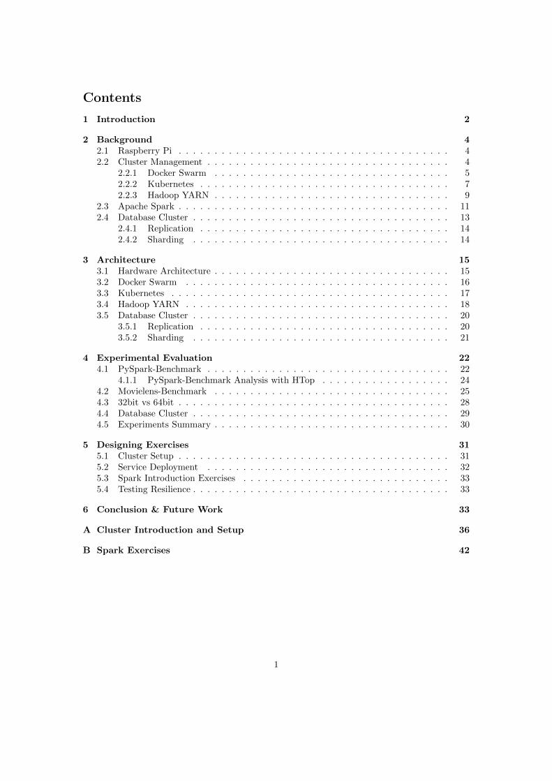
Contents

1 Introduction 2

2 Background 42.1 Raspberry Pi . . . . . . . . . . . . . . . . . . . . . . . . . . . . . . . . . . . . . . 42.2 Cluster Management . . . . . . . . . . . . . . . . . . . . . . . . . . . . . . . . . . 4

2.2.1 Docker Swarm . . . . . . . . . . . . . . . . . . . . . . . . . . . . . . . . . 52.2.2 Kubernetes . . . . . . . . . . . . . . . . . . . . . . . . . . . . . . . . . . . 72.2.3 Hadoop YARN . . . . . . . . . . . . . . . . . . . . . . . . . . . . . . . . . 9

2.3 Apache Spark . . . . . . . . . . . . . . . . . . . . . . . . . . . . . . . . . . . . . . 112.4 Database Cluster . . . . . . . . . . . . . . . . . . . . . . . . . . . . . . . . . . . . 13

2.4.1 Replication . . . . . . . . . . . . . . . . . . . . . . . . . . . . . . . . . . . 142.4.2 Sharding . . . . . . . . . . . . . . . . . . . . . . . . . . . . . . . . . . . . 14

3 Architecture 153.1 Hardware Architecture . . . . . . . . . . . . . . . . . . . . . . . . . . . . . . . . . 153.2 Docker Swarm . . . . . . . . . . . . . . . . . . . . . . . . . . . . . . . . . . . . . 163.3 Kubernetes . . . . . . . . . . . . . . . . . . . . . . . . . . . . . . . . . . . . . . . 173.4 Hadoop YARN . . . . . . . . . . . . . . . . . . . . . . . . . . . . . . . . . . . . . 183.5 Database Cluster . . . . . . . . . . . . . . . . . . . . . . . . . . . . . . . . . . . . 20

3.5.1 Replication . . . . . . . . . . . . . . . . . . . . . . . . . . . . . . . . . . . 203.5.2 Sharding . . . . . . . . . . . . . . . . . . . . . . . . . . . . . . . . . . . . 21

4 Experimental Evaluation 224.1 PySpark-Benchmark . . . . . . . . . . . . . . . . . . . . . . . . . . . . . . . . . . 22

4.1.1 PySpark-Benchmark Analysis with HTop . . . . . . . . . . . . . . . . . . 244.2 Movielens-Benchmark . . . . . . . . . . . . . . . . . . . . . . . . . . . . . . . . . 254.3 32bit vs 64bit . . . . . . . . . . . . . . . . . . . . . . . . . . . . . . . . . . . . . . 284.4 Database Cluster . . . . . . . . . . . . . . . . . . . . . . . . . . . . . . . . . . . . 294.5 Experiments Summary . . . . . . . . . . . . . . . . . . . . . . . . . . . . . . . . . 30

5 Designing Exercises 315.1 Cluster Setup . . . . . . . . . . . . . . . . . . . . . . . . . . . . . . . . . . . . . . 315.2 Service Deployment . . . . . . . . . . . . . . . . . . . . . . . . . . . . . . . . . . 325.3 Spark Introduction Exercises . . . . . . . . . . . . . . . . . . . . . . . . . . . . . 335.4 Testing Resilience . . . . . . . . . . . . . . . . . . . . . . . . . . . . . . . . . . . . 33

6 Conclusion & Future Work 33

A Cluster Introduction and Setup 36

B Spark Exercises 42

1

1 Introduction

Cluster management is part of the syllabus of many data analytics and data sciences modules.However, it is quite hard on the practical side to go into details, as on a typical cloud-basedsystem, many parameters are outside of the control of the user. In the best case, a user canconfigure some basic parameters via a dashboard and the cluster remains an abstract entity.Also, important properties, such as resilience, are hard to investigate, as users are usually notallowed to crash cluster nodes. The goal of this project is to design and develop a cluster madeup of Raspberry Pi computers (see Figure 1). This opens up the possibility to put students infull control of a small cluster in which all the different parameters can be tested and tuned.

This Masterproject is structured into the following tasks:

1. Set up basic infrastructure and compare different solutions

• Connect the hardware, install an operating system, and integrate the Raspberry Pidevices into a network

• Install different cluster management software on top of this infrastructure and figureout which platform is best suited for a Raspberry Pi cluster

• Evaluate different platforms according to their suitability and performance on a Rasp-berry Pi environment

2. Design practical experiments and write the documentation necessary to run the experimentsin a classroom setting

The project report starts with a short introduction about the Raspberry Pi hardware and theused cluster management software to run our architecture, namely: Docker Swarm, Kubernetes,and Hadoop YARN. The main system that will run on top of the cluster is Apache Spark. As afirst step of our practical work, we will elaborate on some of the basics of the interplay betweenour three cluster management software and our Raspberry Pi architectures. This also includesoperating mode and used configuration parameters. To make a comparison of the performanceof the clusters, two different benchmark tests are performed on each architecture. The resultsare visualised and elaborated in the experimental evaluation section. These results serve as adecision support for the selection of the best and most suitable cluster management programfor designing and executing the practical experiments for educational purposes. The report alsoincludes additional experiments like the performance of database clusters on Docker containersand how we have automated the installation process.The practical experiments are designed in a way that each student should be capable of under-standing the key functionalities of a cluster. This includes the possibility to easily setup the fullcluster and the corresponding services like Spark, the underlying distributed file system (DFS),JupyterLab, and Visualizer tools. Also, the students should be able to get a first understandingof the Spark syntax by performing exercises based on PySpark. This is needed to experimentand understand the exercises for testing the resilience of the cluster. The students should beable to see that parallelizing can indeed help to perform computational tasks, which is nearlyimpossible to run on a single machine. By unplugging or plugging in additional Raspberry Pinodes, they should also be capable to see the effects of horizontal scaling and the drawbacks ofa Master-Slave architecture.This project is applied by nature, which means that most references are based on documentationand may not be reliable. Furthermore, due to the rapid development, the provided informationmight be outdated within a few months. This includes the new release of Spark 3.0.0 in mid-June2020 or the start of sales of new Raspberry Pi hardware with 8GB memory in end of May 2020.

2

Figure 1: Final Raspberry Pi Cluster

3

2 Background

This section provides an overview of the Raspberry Pi (RPi) and the software used to connectthem as one cluster. This includes an introduction to the operating modes of each cluster on ahigh level. Furthermore, the cluster computing framework Apache Spark, which runs on top ofeach cluster, will be introduced and elaborated. Last but not least, the section provides the nec-essary theoretical foundations of database clusters that are relevant for additional experiments.

2.1 Raspberry Pi

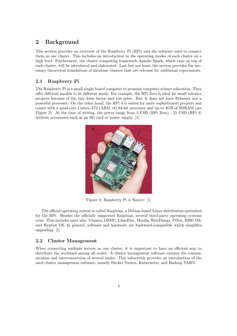
The Raspberry Pi is a small single-board computer to promote computer science education. Theyoffer different models to fit different needs. For example, the RPi Zero is ideal for small roboticsprojects because of the tiny form factor and low price. But, it does not have Ethernet nor apowerful processor. On the other hand, the RPi 4 is suited for more sophisticated projects andcomes with a quad-core Cortex-A72 (ARM v8) 64-bit processor and up to 4GB of SDRAM (seeFigure 2). At the time of writing, the prices range from 5 USD (RPi Zero) - 55 USD (RPi 4)without accessories such as an SD card or power supply. [1]

Figure 2: Raspberry Pi 4, Source: [1]

The official operating system is called Raspbian, a Debian-based Linux distribution optimizedfor the RPi. Besides the officially supported Raspbian, several third-party operating systemsexist. This includes inter alia: Ubuntu, OSMC, LibreElec, Mozilla WebThings, PiNet, RISC OS,and Hypriot OS. In general, software and hardware are backward-compatible which simplifiesupgrading. [1]

2.2 Cluster Management

When connecting multiple servers as one cluster, it is important to have an efficient way todistribute the workload among all nodes. A cluster management software ensures the commu-nication and interconnection of several nodes. This subsection provides an introduction of theused cluster management software, namely Docker Swarm, Kubernetes, and Hadoop YARN.

4

2.2.1 Docker Swarm

Docker is an OS-level virtualization tool for creating and running containers. Similar to hypervi-sors, containers provide an (almost) isolated environment for applications. The main differencebetween hypervisors and containers is their footprint. Containers are more lightweight becausethey run on top of the host machine’s kernel instead of virtualizing the hardware. The advantageis that developers can create, ship, and run many containers on one machine. [2] Figure 3 illus-trates the difference. Containers share the same underlying Linux kernel to keep the performanceimpact as small as possible.

Figure 3: Hypervisor vs. Container

Docker containers are based on the concept of images. Images are read-only templates forcreating docker containers, similar to .ISO files for hypervisors. They can either be downloadedfrom Docker Hub, the largest library of container images or created using a Dockerfile. ADockerfile (no file extension) consists of different layers (commands) that define the steps forbuilding the image. [2] Listing 1 shows a simplified Dockerfile for Spark. The first line defines abase image to build upon, in this case, Ubuntu 18.04. Afterward, Python3 is installed using thepackage manager APT. The last two lines download and run Spark.

# Base Image

FROM ubuntu:18.04

# Install Requirements

RUN apt-get update && apt-get install -y python3

# Download Spark

RUN curl "https://archive.apache.org/dist/spark/spark-2.4.5.tgz" | gunzip

# Run Spark

CMD ["spark-2.4.5/bin/spark-class", "org.apache.spark.deploy.master.Master"]

Listing 1: Dockerfile Example

The default Docker Engine executes containers on one host only. However, there is a built-incontainer orchestration feature called Swarm. A Swarm consists of multiple Docker hosts anddistributes containers automatically. Each Swarm has at least one manager with the possibility ofadding as many workers as needed. But, the ability to deploy containers to the Swarm cluster isrestricted to the manager. If the manager fails (assuming a single-manager), the services continueto run but a new cluster has to be created eventually. [2] Figure 4 illustrates the dependencies. Itis important to note that containers are not ”copied” between the nodes. Each node downloads

5

the image from a registry (e.g. Docker Hub).

Figure 4: Docker Swarm Schema

The advantage of Docker Swarm (e.g. compared to Kubernetes) is its simplicity. Replicationand load balancing works right out of the box without having to configure anything. For example,Figure 5 (left) shows two NGINX webservers running on two different nodes. The requests areautomatically load-balanced between these two. In the case of node failures (Figure 5, right), thecontainers are automatically started on a different node. Since there is only one working nodeleft, the container is recreated on the remaining node.

Figure 5: Left: Working Swarm Cluster, Right: Failed Node

Unfortunately, there are also downsides and risks when using Docker. On the one hand,there are justified security concerns because of the semi-isolated environment. This is not a mainconcern for this project. On the other hand, persistent storage in Docker is complicated. Dueto the stateless nature of Docker containers, persistent data is stored separately in a Dockervolume. The volumes are stored on the host machine and can be mounted by the containers.This is problematic because a Swarm consists of multiple hosts and volumes are restricted to onehost. If a container is moved to another host, it mounts the volume from the new host whichmight contain different data or none at all. To get around this problem, it is common practiceto use external storage such as cloud-storage [3, 4] or a dedicated storage-server. [2] However,to keep this project self-contained and independent of cloud providers, we use Gluster [5] as analternative. Gluster is an open source, distributed file system capable of replicating files acrossnodes. The file location is hidden from the user and stored in ”bricks” on different servers. Thebricks are managed by a Gluster volume which internally ensures certain requirements such asreplication. [5] Figure 6 illustrates the difference between local, shared and distributed storage.

6

Local storage can’t be accessed across hosts which limits its use in a multi-server setup. Sharedstorage is the de facto standard for container orchestration but requires a dedicated, reliable andhigh-performance storage server. Gluster stores the data in a distributed manner and does notrequire a central server (at the cost of performance).

Figure 6: Local Storage vs. Shared Storage vs. Gluster

2.2.2 Kubernetes

Kubernetes is Greek for Helmsman (the person who steers a ship), is an open-source production-grade container orchestration system. It was originally developed by Google and is now main-tained by the Cloud Native Computing Foundation [6]. Kubernetes (or K8s) is a managementsystem that runs Docker images in objects called Pods.

Kubernetes objects In the Kubernetes System there exist persistent entities called Kuber-netes Objects [7] and they represent the state of the cluster.

Pods The system has an abstraction grouping that consists of one or more co-located containerscalled pods. Pods are created using a yaml (or json) configuration file to specify the way thatthey are deployed. Pods can be deployed in 3 different kinds of way, namely: Deployments,StatefulSets, and DaemonSets.

• Deployments will create pods to a specified number of replications and will be allocatedpods to nodes in a resource-efficient way.

• DaemonSets will replicate the pod to all Nodes and will add/remove pods as nodes areadded or removed.

• StatefulSets are used when a persistent state is required, each node is named with anappended index e.g mypod-0, mypod-1, mypod-3 etc.

Services This is an abstract way to expose a pod (or set of pods) as a network service. Theyare needed for inter pod communication as well as for exposing pods to outside of the cluster.They also use load balancing that operates in a round-robin manner to balance network trafficfrom the requesting address to among the pods [8].

Volumes When a pod restarts the internal storage is not persisted, therefore to have persis-tence storage, volumes mount storage to specific mount points within the container which aredefined in the pod configuration. There are quite a few storage options available, we choose tostick with GlusterFS since we had already used it with Docker [9].

7

Namespaces These allow resource partitioning into non-overlapping sets and are intended tobe used in a production environment where multiple teams are working on the same cluster [10].

The layout of Kubernetes is similar to Docker Swarm, where there is a Master and WorkerNodes. When initializing the Master it returns a join token that is used to add Worker Nodes.After creating a replica set of pods, to communicate with our application, we create a servicethat exposes the application as a network service (Figure 7). This service load balances theexternal requests from 8080 to the pods on 80. Internal communication between pods are doneon virtual IPs that are set up by the pod network (Figure 8).

Kubernetes can pull images directly from Docker Hub to set up pods, for example, to pullthe nginx image and expose port 80, run: kubectl run nginx --image=nginx --port 80 orall the specification can be created in a yaml file and deploy it this way: kubectl create -f

nginx.yaml

Figure 7: A service in Kubernetes

Figure 8: Kubernetes pod interaction [11]

8

2.2.3 Hadoop YARN

Hadoop is a Java-based software framework and is freely available as Apache source code. Thename “Hadoop” goes back to a small toy elephant of the inventor Doug Cutting’s son. The ele-phant is still present in the Hadoop logo today. The following three core components of Hadoopwere used in this project:

• Hadoop CommonHadoop Common provides the basic functions and tools for the other building blocks of thesoftware. These include, for example, the Java archive files and scripts for starting the software.Communication between Hadoop Common and the other components is via interfaces. Thesecan be used to control access to the underlying file systems or the communication within clusters.

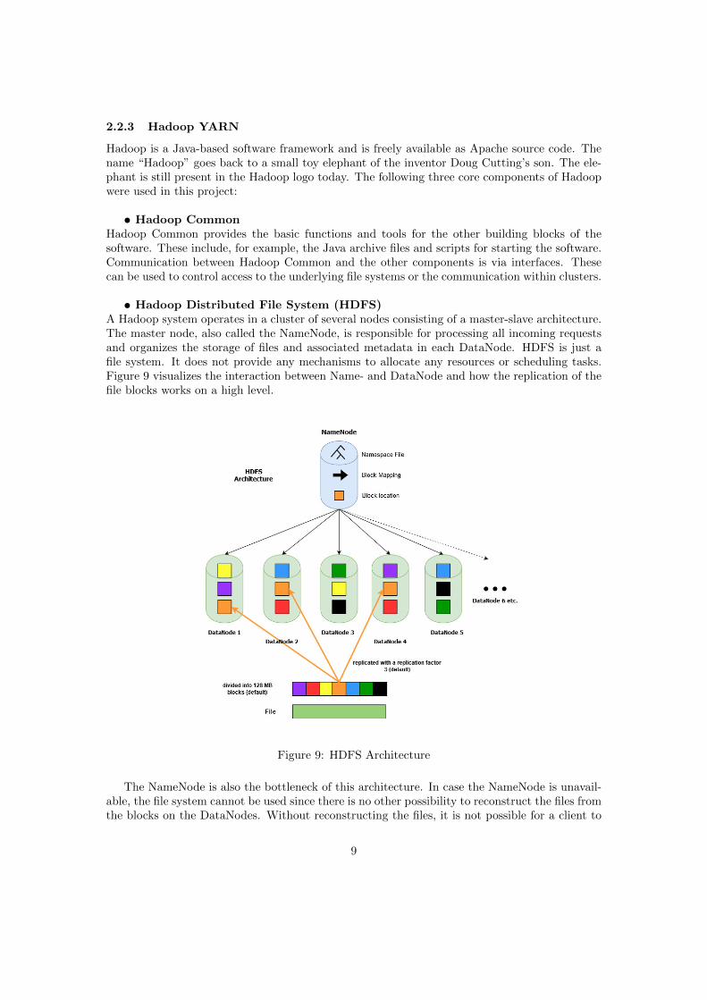
• Hadoop Distributed File System (HDFS)A Hadoop system operates in a cluster of several nodes consisting of a master-slave architecture.The master node, also called the NameNode, is responsible for processing all incoming requestsand organizes the storage of files and associated metadata in each DataNode. HDFS is just afile system. It does not provide any mechanisms to allocate any resources or scheduling tasks.Figure 9 visualizes the interaction between Name- and DataNode and how the replication of thefile blocks works on a high level.

Figure 9: HDFS Architecture

The NameNode is also the bottleneck of this architecture. In case the NameNode is unavail-able, the file system cannot be used since there is no other possibility to reconstruct the files fromthe blocks on the DataNodes. Without reconstructing the files, it is not possible for a client to

9

read the blocks since the NameNode cannot communicate the block locations to the client. [12]But Hadoop provides several mechanisms for guaranteeing high-availability. This can be doneby e.g. configuring Standby NameNodes or Secondary NameNodes.

By default, a block size in a data node is 128MB. HDFS blocks are large compared to diskblocks, and the reason is to minimize the cost of seeks. By making a block large enough, thetime to transfer the data from the disk can be made to be significantly larger than the time toseek to the start of the block. [12] In a multi-node Hadoop cluster, the blocks are replicatedthree times by default, which provides fault tolerance in case one DataNode is unavailable.

• Yet Another Resource Negotiator (YARN)YARN is Hadoop’s Resource Manager and is responsible for allocating the requested resources(CPU, memory) of a Hadoop cluster of different jobs. This allows certain jobs to be allocatedmore or less resources, which can be configured per application and user.

Figure 10: Typical YARN Cluster

There are four important components in a YARN-cluster: Resource Manager, NodeManager,Application Master and, several containers. The Resource Manager runs on the MasterNode andmanages the scheduling of computing resources to applications. It optimizes cluster utilization interms of memory, CPU cores, fairness, and SLAs. One main component of the Resource Manageris the scheduler, which does not provide any guarantee for job completion or monitoring. Itonly allocates the clusters’ resources [13]. In Figure 10 it is illustrated that every WorkerNodecontains a NodeManager, which acts as the ResourceManager’s monitoring and reporting agent.The NodeManager sends heartbeat signals to the ResourceManager to update its health status.An ApplicationMaster is scheduled by the ResourceManager for each separate application tonegotiate resources and to work together with the NodeManager to perform and monitor tasks.Containers are controlled by the NodeManagers and are responsible for assigning the resources

10

provided by the system to each application. A container grants rights to an ApplicationMasterto use a specific amount of resources of a specific host. An ApplicationMaster is considered asthe first container of an application and it manages the execution of the application logic onallocated containers. [13]

YARN uses queues to determine the capacities of the systems for individual tasks. There arethree different scheduling mechanisms to allocate resources for submitted jobs to YARN: FIFO,Capacity, and Fair Schedulers. The scheduling mechanism will be FIFO for this project. Onlyone job is submitted, which should use all of the resources of the cluster.

2.3 Apache Spark

On top of each cluster setup, Apache Spark is running. This computing framework will also beused to execute benchmark tests to compare the performance between each cluster. The providedtheoretical foundations are based on the lecture ”Big-Data Analytics” at the University of Zurich[14] and the textbook ”Learning Spark” from Holden Karau et. al. [15]Apache Spark offers the ability to run computations in memory and parallel in a cluster whiletrying to avoid writing to a hard disk. One of the main components of Spark is Spark Core.Spark Core contains the basic functionality of Spark, including components for task scheduling,memory management, fault recovery, interacting with storage systems, and more. Spark Coreis also home to the API that defines resilient distributed datasets (RDDs), which are Spark’smain programming abstraction [15]. This is a concept to distribute data over several nodes andprocess them in parallel. RDD stands for:

• Resilient: Fault-tolerant, so that disastrous or broken partitions can be restored in case ofdamaged SparkWorkers

• Distributed: Data is distributed in partitions across different nodes in a cluster

• Dataset: Collection of partitioned data

RDDs and DataFrames can be created from external data sources (e.g. HDFS, SQL) orfrom internal process steps. Dataframes are the easiest and most efficient abstraction. One cancompare Dataframes with a traditional table with columns and rows, which is generally used forhandling workflows with structured data. If the data is unstructured (has no schema) and thedata needs to be manipulated in non-standard ways, one should use RDD’s [14]. An importantcharacteristic of Spark is the lazy evaluation. It always waits until the last moment to executea computation by building efficient execution plans. This also simplifies the restart after losinga data partition, since every partition contains information for recalculating it.

On a high level, every Spark application consists of a driver program that launches variousparallel operations on a cluster. The driver program contains the application’s main functionand defines distributed datasets on the cluster, then applies operations to them. In distributedmode, Spark uses a master/slave architecture with one central coordinator and many distributedworkers. The central coordinator is called the driver. The driver communicates with a potentiallylarge number of distributed workers called executors. The driver runs in its own Java processand each executor is a separate Java process. A driver and its executors are together termeda Spark application [15]. Spark can also run over cluster managers like Hadoop YARN or asimple cluster manager included in Spark itself called the Standalone Scheduler. The interactionbetween all the above-mentioned components is visualized in Figure 11 below.

11

Figure 11: Cluster Overview Spark [15]

Spark uses a few ports for communication, therefore, these ports must be open for properfunctionality. The block master and spark driver services set a random port every time they start,this could pose a communication problem when running under a strict firewall, in the case theseports must be set manually for example by spark-submit --conf spark.driver.port=4102.The used ports by spark are listed in Table 1 below.

Name PortSpark Master 7077Spark Worker randomMaster-UI 8080Worker-UI 8081Block Master randomSpark Driver random

Table 1: Ports used by Spark [16]

RDDs offer two types of operations: transformations and actions. Transformations constructa new RDD from a previous one. For example, one common transformation is filtering data thatmatches a predicate. Actions, on the other hand, compute a result based on an RDD, and eitherreturn it to the driver program or save it to an external storage system (e.g. HDFS) [15]. ASpark program implicitly creates a logical directed acyclic graph (DAG) of operations. Whenthe driver runs, it converts this logical graph into a physical execution plan [15]. For example,Figure 13 visualized the DAG from chapter 4.1 ”PySpark-Benchmark”. Each job consists ofone or many stages, whereas each stage consists of one or many tasks. For example, our usedshuffle benchmark from chapter 4.1 consists of 5 jobs, split into a total of 11 stages and againdivided into a total of 1062 tasks. The visualised DAG from the ”inner-join” benchmark is, asit is visualized in Figure 12, 1 of the total of 5 shuffle benchmark jobs, split into 3 stages (stage5,6, and 7) and into a total of 220 tasks.

12

Figure 12: Completed Stages for ”Inner-join” benchmark

Figure 13: DAG for ”Inner-Join” benchmark

2.4 Database Cluster

This section is part of additional experiments that we have done out of interest. As alreadymentioned, Spark can use external data sources such as a database (SQL and NoSQL). In casea database reaches its limits e.g. because of performance or other limitations, a database clustermight be an option to consider. So, we tested the performance and the behavior of a traditionaldatabase on one of our cluster setup.

13

Generally, a distinction is made between horizontal and vertical scaling. Vertical scaling extendsthe server e.g. by adding an additional CPU or memory. Horizontal scaling, on the other hand,involves adding more servers and dividing the workload accordingly. [17] Figure 14 visualizes thetwo approaches. This project will focus on horizontal scaling of relational databases.

Figure 14: Horizontal vs. Vertical Scaling

2.4.1 Replication

Replication is one of the most straight forward scaling methods. Typically, a database is repli-cated on different nodes (e.g. master-slave) with some restrictions on write operations (e.g.read-only slaves). This is because relational DBMS are based on ACID (Atomicity, Consistency,Isolation, and Durability) transactions and write queries on different nodes might break theconsistency. However, for read-heavy applications, replications can increase performance with-out the need for changing the internal database structure. Furthermore, replications provide abackup in case of a node failure e.g. with automatic failovers. In summary, replications improvepredominantly read-only queries and provide high-availability in case of a node failure. [17]

2.4.2 Sharding

At a large scale, replication might not be sufficient which is when sharding should be considered.The problem with replication is that it is not infinitely scalable. At some point, a single serverreaches its limits. With sharding, the records are split by a key and stored on different servers[17]. For example, Instagram engineers released an article in 2012 [18] where they explain theirdatabase scaling approach. They had to store 25 photos every second and decided to shard byuser. With this approach, photos are stored on different servers depending on the user. Figure15 illustrates the ”sharding by user” approach.

Figure 15: Sharding Example

14

3 Architecture

The following section provides an introduction to the specific architecture of our physical setup.This includes details about the corresponding master-slave architecture, requirements and cer-tain configuration parameters of our setup. Last but not least, we provide details about ourPostgreSQL based database cluster.

3.1 Hardware Architecture

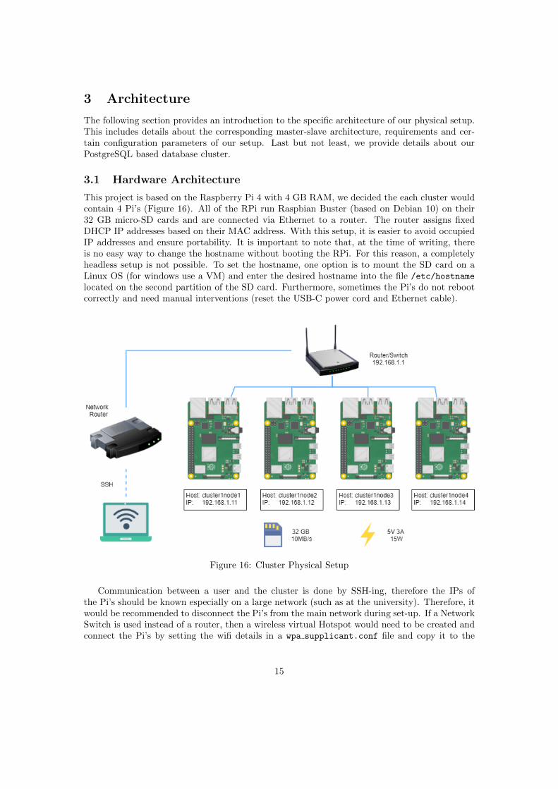
This project is based on the Raspberry Pi 4 with 4 GB RAM, we decided the each cluster wouldcontain 4 Pi’s (Figure 16). All of the RPi run Raspbian Buster (based on Debian 10) on their32 GB micro-SD cards and are connected via Ethernet to a router. The router assigns fixedDHCP IP addresses based on their MAC address. With this setup, it is easier to avoid occupiedIP addresses and ensure portability. It is important to note that, at the time of writing, thereis no easy way to change the hostname without booting the RPi. For this reason, a completelyheadless setup is not possible. To set the hostname, one option is to mount the SD card on aLinux OS (for windows use a VM) and enter the desired hostname into the file /etc/hostname

located on the second partition of the SD card. Furthermore, sometimes the Pi’s do not rebootcorrectly and need manual interventions (reset the USB-C power cord and Ethernet cable).

Figure 16: Cluster Physical Setup

Communication between a user and the cluster is done by SSH-ing, therefore the IPs ofthe Pi’s should be known especially on a large network (such as at the university). Therefore, itwould be recommended to disconnect the Pi’s from the main network during set-up. If a NetworkSwitch is used instead of a router, then a wireless virtual Hotspot would need to be created andconnect the Pi’s by setting the wifi details in a wpa supplicant.conf file and copy it to the

15

micro-SD cards. Once the Pi’s are on a local network, nmap can be used to scan the network toget the IP addresses of the Pi’s. This is why we recommend using a home router and definingstatic IP leases in the DHCP settings. If the router does not support this, one option would beto flash OpenWrt onto the router.The Pi’s are powered by the USB-C port, they can also be powered by purchasing a PoE hatand using a router the supplies Power over Ethernet, this creates a much cleaner design as thereare less cables to handle. The USB-C power-in must be at least 15 Watts, therefore a laptopcannot be used to power a Pi. Also, an adequately long power strip is required since the poordesign of the official power adapters can block adjacent sockets.The cluster is setup such that node 1 is the master and the other nodes are the slaves/workers,we decided to make the master also do work, this means that a worker application will also berunning on the master. In real-world applications, this practice is not advised, but there is alsothe option to have to place the master on a laptop or in a VM, this way node 1 would have moreresources to work with when under load.

3.2 Docker Swarm

Docker runs on every major operating system and CPU architecture. This includes x86 64,arm32, arm64, mips and others. However, it must be remembered that Docker depends on thehost machine’s kernel and does not virtualize the hardware. As a consequence, docker imageshave to be built for each CPU architecture separately. [2] At the time of writing, building multi-arch images is still experimental and most images on Docker Hub only support a subset of CPUarchitectures.

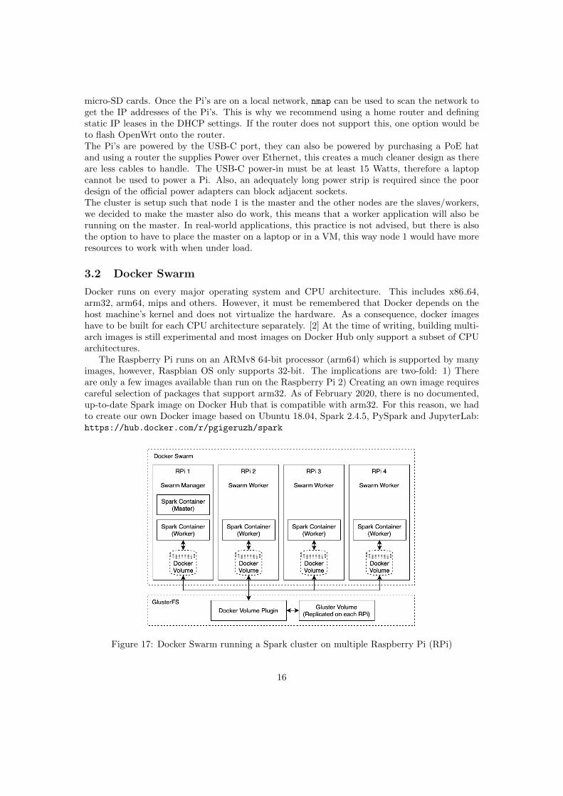
The Raspberry Pi runs on an ARMv8 64-bit processor (arm64) which is supported by manyimages, however, Raspbian OS only supports 32-bit. The implications are two-fold: 1) Thereare only a few images available than run on the Raspberry Pi 2) Creating an own image requirescareful selection of packages that support arm32. As of February 2020, there is no documented,up-to-date Spark image on Docker Hub that is compatible with arm32. For this reason, we hadto create our own Docker image based on Ubuntu 18.04, Spark 2.4.5, PySpark and JupyterLab:https://hub.docker.com/r/pgigeruzh/spark

Figure 17: Docker Swarm running a Spark cluster on multiple Raspberry Pi (RPi)

16

Figure 17 shows the architecture of our setup. The Swarm manager runs a Spark master anda Spark worker. All other nodes act as Spark workers. It is important to note that everythingruns within an overlay network with published ports for external communication. But, becauseof Spark, it is not possible to connect to the Spark cluster from outside the network. The onlypossible way to interact with the cluster is from within another container that has access tothe overlay network. This means that everything, including the spark-submit client, has to becontainerized. For persistent storage, Gluster synchronizes the data across all nodes. Togetherwith a docker volume plugin, it is possible to mount the Gluster volume as a docker volume. Intheory, it would be possible to run a Hadoop cluster on top of Gluster but the docker volumeplugin does essentially the same with less overhead.

3.3 Kubernetes

Kubernetes runs everywhere where Docker can run [19]. When Docker images are built, theyuse the host system’s kernel, this means that, for example, an image built on x86 32 cannot runon arm 32. However, since we already built a Spark image on arm 32 for the Docker Swarm, wecan use the same image for our Kubernetes Cluster.

The architecture for the Kubernetes cluster is quite similar to that of Docker Swarm on a highlevel. Spark runs in a container that is replicated across all nodes. By default, Kubernetes doesnot allow pods to run on the master node. Since we want to also utilize the master node, weenabled scheduling of pods on the master node [20]. Like Docker Swarm, the master node runsthe Spark Master (spark-submit) as well as a Spark Worker. We install Gluster the same way,with the exception that instead of the volume plugin, we create a service opening a specified portto allow communication between the Gluster endpoints on each raspberry pi. In our deploymentyaml file we specify that we want to mount the Gluster shared volume inside the container.

Architecture Components A Kubernetes cluster runs containerised applications on workernodes, therefore naturally every cluster must have at least one worker node. Kubernetes requirecertain core components to operate [22] Figure 18, these are as follows:

• etcd: This component stores configuration data as consistent and highly-available keyvalues that can be accessed through the Kubernetes API Server.

• API Server: This component is the front-end of the Kubernetes control plane that exposesthe Kubernetes API. It facilitates communication between the various components andmaintains the cluster’s overall health. Controller Manager: This component runs controllerprocesses to ensures that the current state matches the desired state e.g the node controlleris responsible for noticing and responding when nodes go down.

• Scheduler: This component ensures that Posts are matched to nodes so the Kubelet canrun them. When Pods are created it determines the best Node for that Pod to run on.

• Kubelet: This component runs on each node and ensures that the containers are runningin a Pod. Pod specifications are sent from the API Server to the Kubelet which managespods running on its node.

Kubernetes on Debian There are several nuances running Kubernetes on the RaspberryPi’s. Since the Raspbian OS is Debian based it inherits any Debian OS specific issues, runningKubernetes requires the use of legacy iptables [23], since the latest Debian build uses iptables

17

Figure 18: Kubernetes Architecture [21]

version 1.8.x which breaks compatibility with Kubernetes. This issue is not documented in theofficial installation guide.

3.4 Hadoop YARN

Figure 19 shows the YARN architecture of our setup. The MasterNode (RP0) runs as Sparkmaster and also as Spark worker while all other nodes (RP1-3) act only as Spark workers. Incontrast to the upper two architectures, the Spark setup files are only configured on the masterrespectively on the cluster. Thus, there is no local Spark installation needed on the Workers.When submitting a spark application, there is either the possibility to enter resource requirementsvia command line (Listing 2) or defining it in the spark-defaults.conf file (Table 2). If a parameteris not set at all, it will use a default or a max value to execute a Spark-job. In certain cases ofour project, this has resulted in ”out-of-memory” errors for CPU-intensive applications.

spark-submit --master yarn --deploy-mode cluster --num-executors 14

--driver-memory 2g --executor-memory 1g --executor-cores 1

benchmark-shuffle.py hdfs://192.168.1.187:9000/pyspark-benchmark/file

Listing 2: Spark Submit Example on YARN

18

There are many parameters in Hadoop and Spark, which can be set individually. The detailsof the relevant configurations in our project can be found in Table 2 and Table 3 below. Thedifficulty lies in the fact that when defining the Spark parameters, the Yarn parameters mustbe taken into account. For example, the defined spark.driver / executor.memory + spark.driver/ executor.memoryOverhead cannot exceed the configured yarn.nodemanager.resource.memory.Also, the number of cores needs to be considered to have an efficient workload distributionamong all nodes. If one of the parameters is not properly set for a raspberry pi environment, theexecution of the job will not start and will return an error. In the following part, the interplaybetween Spark and YARN will be explained when submitting a job.

Figure 19: YARN cluster running a Spark cluster on multiple Raspberry Pi

As soon as a client submits a Spark job to the Master, the NameNode will check various thingslike permissions to read/write or if the path is valid. If the checks are successful, the job will getan application-ID and goes into the job queue. All needed information are written into a templocation in our case in ”/hdfs/tmp”. This can be specified in the Hadoop configuration file ”core-site.xml”. As soon as the resource files are uploaded and the application is submitted, the job willchange into an ”ACCEPTED” state. The input data file should be already loaded into HDFS,before executing the Spark Job. The YARN Resource Manager schedules a Spark ApplicationMaster with the corresponding Spark Driver on a random WorkerNode. The Application Mastercollects the relevant details and communicates with the NodeManager, which evaluates wherethe required input data blocks are located or how much resources (CPU, cores, memory) arerequired to compute the job. This information is sent via Application Master to the ResourceManager. The Resource Manager sends the allocation request to the NodeManagers. In the end,the Application Master launches and monitors the Spark executors until the execution succeedsor fails. The final state of the submitted job will change to ”SUCCEEDED” or ”FAILED”.After or during the execution of the job, the details can be checked in the logs of the Hadoop-Web-UI running on port 8088. This includes e.g. launching of containers, resource utilization ofthe executors or task-tracking on specific nodes.

19

Config file Property Default Value Used Value Comments

yarn-site.xml

yarn.scheduler.minimum-allocation-mb 1024 64 Minimum allocation for every containerrequest at the Resource Manager

yarn.scheduler.maximum-allocation-mb 8192 2048 Maximum allocation, relevantwhen scheduling Application Master

yarn.nodemanager.resource.memory-mb 8192 4096 Node has in maximum 4GB RAM availableyarn.scheduler.minimum-allocation-vcores 1 1 Node must allocate 1 core for an applicationyarn.scheduler.maximum-allocation-vcores 4 4 Node can allocate up to 4 cores for

an application per workerhdfs-site.xml

dfs.replication 3 4 Replication factor of the blocksdfs.blocksize 128m 64m Blocksize of the datanodes

core-site.xml hadoop.tmp.dir /tmp/hadoop-user /hdfs/tmp Location where client uploads resource file

Table 2: Hadoop parameters in YARN cluster

Config file Property Default Value Used Value Comments

spark-defaults.conf

spark.master none yarn YARN-cluster is the spark-masterspark.executor.memory 1024 640 Each spark executor has a reserved overhead of 384MB.

One executor should use 640+384=1024MB RAM per corespark.driver.memoryOverhead 384 1024 Needed in case of CPU intensive applications

Table 3: Spark parameters in YARN cluster

3.5 Database Cluster

One of the most popular and advanced open source relational database is PostgreSQL [24] whichis why we use it in this project. The advantages of PostgreSQL are robustness, reliability,and performance. Furthermore, PostgreSQL includes basic clustering features out of the box.It should be noted that there are PostgreSQL forks (e.g. Citus or Patroni) that simplify theclustering process. [24] However, we were not able to compile them on ARM which is why thefollowing sections are based on plain PostgreSQL.

3.5.1 Replication

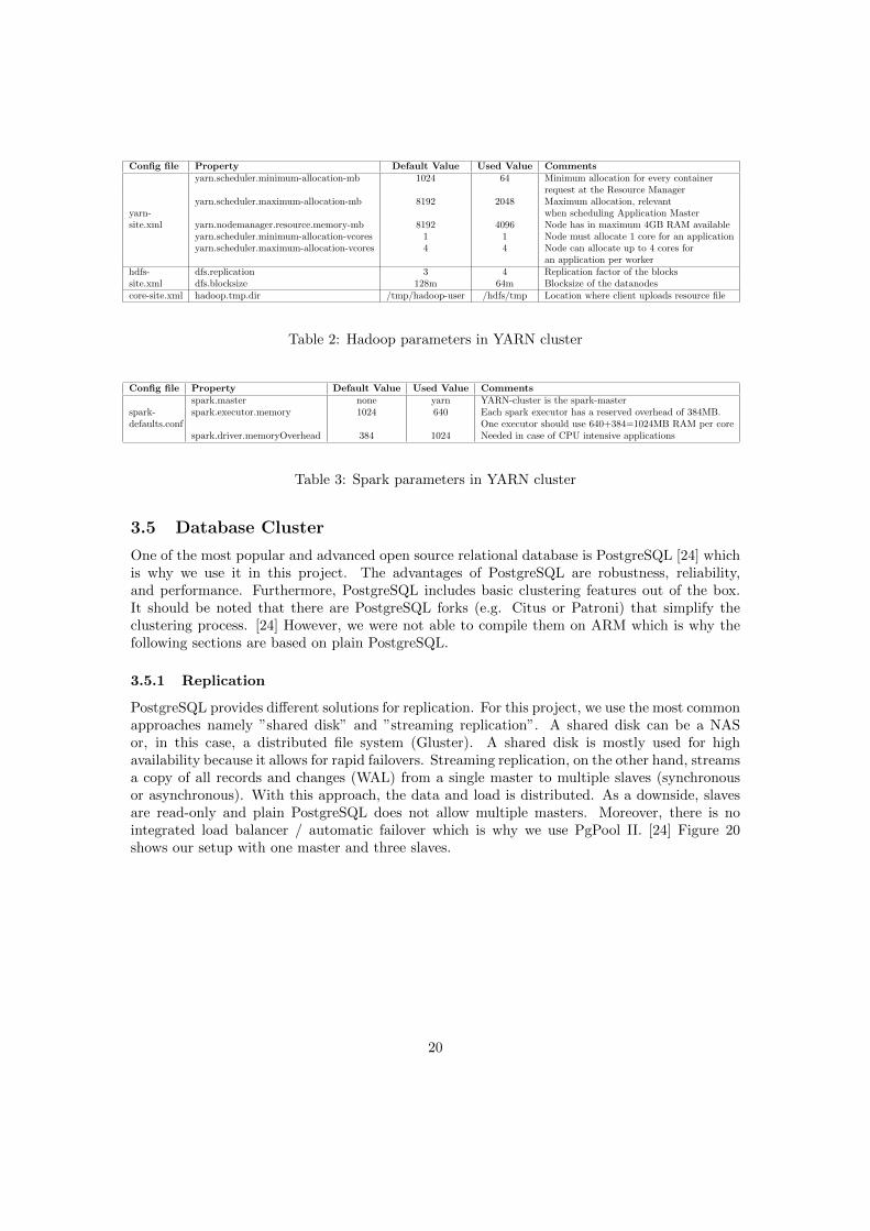
PostgreSQL provides different solutions for replication. For this project, we use the most commonapproaches namely ”shared disk” and ”streaming replication”. A shared disk can be a NASor, in this case, a distributed file system (Gluster). A shared disk is mostly used for highavailability because it allows for rapid failovers. Streaming replication, on the other hand, streamsa copy of all records and changes (WAL) from a single master to multiple slaves (synchronousor asynchronous). With this approach, the data and load is distributed. As a downside, slavesare read-only and plain PostgreSQL does not allow multiple masters. Moreover, there is nointegrated load balancer / automatic failover which is why we use PgPool II. [24] Figure 20shows our setup with one master and three slaves.

20

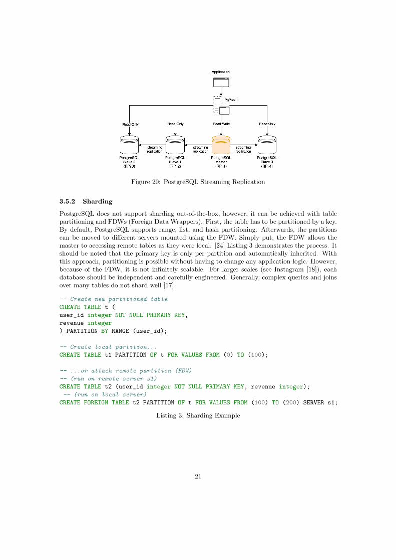
Figure 20: PostgreSQL Streaming Replication

3.5.2 Sharding

PostgreSQL does not support sharding out-of-the-box, however, it can be achieved with tablepartitioning and FDWs (Foreign Data Wrappers). First, the table has to be partitioned by a key.By default, PostgreSQL supports range, list, and hash partitioning. Afterwards, the partitionscan be moved to different servers mounted using the FDW. Simply put, the FDW allows themaster to accessing remote tables as they were local. [24] Listing 3 demonstrates the process. Itshould be noted that the primary key is only per partition and automatically inherited. Withthis approach, partitioning is possible without having to change any application logic. However,because of the FDW, it is not infinitely scalable. For larger scales (see Instagram [18]), eachdatabase should be independent and carefully engineered. Generally, complex queries and joinsover many tables do not shard well [17].

-- Create new partitioned table

CREATE TABLE t (

user_id integer NOT NULL PRIMARY KEY,

revenue integer

) PARTITION BY RANGE (user_id);

-- Create local partition...

CREATE TABLE t1 PARTITION OF t FOR VALUES FROM (0) TO (100);

-- ...or attach remote partition (FDW)

-- (run on remote server s1)

CREATE TABLE t2 (user_id integer NOT NULL PRIMARY KEY, revenue integer);

-- (run on local server)

CREATE FOREIGN TABLE t2 PARTITION OF t FOR VALUES FROM (100) TO (200) SERVER s1;

Listing 3: Sharding Example

21

4 Experimental Evaluation

This project uses two benchmarks to evaluate the performance of the Spark cluster. The firstbenchmark is artificial and generates randomized test data. The second benchmark is based ona public data-set and focuses on real-world performance. The following sections describe thebenchmarks and show the performance for each cluster management software. Furthermore, abenchmark for the database cluster is provided at the end.

4.1 PySpark-Benchmark

The PySpark-Benchmark [25] is a lightweight benchmark for PySpark. Contrary to full-blownbenchmarks such as Spark-Bench [26], it is easy to deploy and has an understandable source-code. Unlike Spark-Bench, it can generate any amount of data and does not require hundreds ofgigabytes of files. This is especially important because of the limited resources of the RPi.

Table 4 shows the first two rows of the generated data set. The value field is a randomlygenerated UUID on which the other fields are based on. The prefix fields are substrings directlytaken from the UUID whereas the float val/integer val are first converted into the respectivedata type. [25]

value prefix2 prefix4 prefix8 float val integer valc72c3c6c791e4b6cb7abb38c0a8f1a7e c7 c72c c72c3c6c 484185.6054 484185b49a045cf168443b99806a9f59f9510c b4 b49a b49a045c 779722.1738 779722

...

Table 4: Generated Test Data Example

The benchmark itself is divided into seven subcategories. The first four categories include”Group By and Aggregate”, ”Repartition”, ”Inner Join”, and ”Broadcast Inner Join”. Thesecategories cover common (distributed) PySpark operations on a data frame. The last threecategories include ”SHA-512 hashing”, ”Estimating Pi with data frame”, and ”Estimating Piwith random samples”. These operations are primarily CPU focused and rely less on I/O. [25]

The ”Group By” benchmark groups the dataframe (see Table 4) by prefix2 and aggregatesthe other variables using the sum/count. Similarly, ”Inner Join” and ”Broadcast Inner Join”creates a new table aggregated by prefix2 and joins the original dataframe. For the ”Repartition”benchmark, the prefix4 is used to partition the table. The ”SHA-512” benchmark calculates theSHA-512 hash for each value field in the dataframe. ”Calculate Pi” is based on a Monte Carloexperiment to estimate Pi based on random samples. Additionally, ”Calculate Pi dataframe”appends the random samples to the dataframe letting Spark optimize the result aggregation.

For this project, we use a 71MB (1000000 rows) file and 40000000 random samples for thePi estimation. These numbers are derived empirically with the aim of having approx. 5 minutesper benchmark run. The results can be found in Figures 21 and 22. Both, Kubernetes andSwarm, are similar in performance due to having the same underlying container technology(Docker). YARN, on the other hand, is considerably slower. Our hypothesis is that the overheadis due to the fully distributed mode of YARN (Docker has to run as standalone mode). In thismode, YARN has spark installation only on master whereas Docker has spark installed on everynode. Interestingly, more workers increase the performance of all systems although not linearly.However, the overall performance is not competitive. For comparison, a Macbook Pro 2018 (2.2GHz 6-Core Intel Core i7, 16 GB 2400 MHz DDR4) is more than twice as fast as four RPi evenon CPU-intensive tasks.

22

Figure 21: PySpark-Benchmark Results Overall

Figure 22: PySpark-Benchmark Results Per Category

23

4.1.1 PySpark-Benchmark Analysis with HTop

As we have seen in the PySpark-Benchmark test, the performance of YARN is lower than forKubernetes and Swarm. This section provides a detailed analysis of the resource utilizationvia HTop. For each cluster, we ran the PySpark-Benchmark test again and checked the resourceutilization for the following states: Master idle, Master shuffle, Master CPU, Worker idle, Workershuffle, and Worker CPU. Shuffle and CPU refer to the two executed benchmark scripts, whereasidle is the resting state when the architecture of each cluster is running but no Spark job issubmitted and executed. For the idle state, we recorded the HTop results after 30 minutes. Forthe shuffle and CPU benchmark, we tried to record the results when the capacity utilization wasat its highest. The results for each cluster are listed in the Tables 5, 6 and Table 7 below.

Kubernetes master workerState idle shuffle cpu idle shuffle cpu

Core 1 4.0 95.6 81.5 3.9 67.1 67.5Core 2 6.5 93.0 79.9 1.3 81.4 64.5Core 3 8.4 99.4 94.8 3.2 71.9 64.5Core 4 4.0 93.5 80.4 2.6 67.3 63.6

Memory 0.86G 1.12G 0.83G 0.44G 1.33G 1.14G

Table 5: HTop capacity utilization [%] for Kubernetes

Swarm master workerState idle shuffle cpu idle shuffle cpu

Core 1 0.0 72.7 71.9 5.1 67.3 99.3Core 2 0.6 80.9 76.8 5.2 68.2 70.8Core 3 0.0 74.8 75.8 3.2 69.9 71.1Core 4 3.2 67.5 98.1 1.9 88.0 72.8

Memory 0.45G 1.14G 0.87G 0.28G 1.04G 1.00G

Table 6: HTop capacity utilization [%] for Swarm

YARN master workerState idle shuffle cpu idle shuffle cpu

Core 1 5.8 99.4 99.4 1.3 100.0 96.1Core 2 0.6 99.4 93.8 0.0 100.0 51.0Core 3 0.6 100 91.2 3.2 100.0 82.5Core 4 0.0 99.4 98.1 1.9 100.0 88.2

Memory 0.54G 1.93G 0.85G 0.30G 1.36G 1.02G

Table 7: HTop capacity utilization [%] for YARN

24

There are four cluster-state constellations which are at their limit. The Kubernetes andYARN master while shuffling, the YARN-master during the execution of the CPU benchmark,and especially the YARN workers while shuffling. The YARN worker node, which returns a100% utilization on all cores, includes the scheduled Application Master, which monitors the jobexecution on all containers. The Application Master has a configured capacity of 2048MB sincethere are additional services running to track and monitor the individual spark tasks. This isthe only exception in the configuration of all clusters. The agreed value for the executors in thisproject is 1024MB per core. Increasing this value would further complicate a clear comparisonbetween all clusters. This also means that our YARN cluster is operating with 15 cores insteadof 16 cores as it’s the case for Swarm and Kubernetes. This surely has also an impact on theperformance of the YARN-cluster.

There are other factors that have an impact on the performance of YARN. However, findinga particular cause is difficult due to the inherently different architecture of YARN and Swar-m/Kubernetes. For this reason, we can only guess the reasons:

• Jobs are relatively small, therefore, the overhead of YARN is too big

• Executor memory for YARN (640MB + 384MB overhead) is not the right configurationfor an efficient job execution. But, this is needed to use 15 cores and a total of 16GB ofmemory in our YARN cluster

• The Resource Manager nor the Application Master (2048MB) receive enough computa-tional power

• Swarm and Kubernetes might simply be more efficient and lightweight

• YARN has Spark installation only on master, whereas the other two architectures haveSpark installed on every node

4.2 Movielens-Benchmark

MovieLens is a common data set used in Big Data testing. We are using the 20-m data set thatcontains 20,000,263 ratings across 27,278 movie created from 138,493 users form the period 1995to 2015. We are using the movies file and the ratings file. The movie file contains the movie id,its title and the genres of that movie separated by pipes and the reviews file contains the userid, movie id, rating (between 0-5) and the timestamp in epoch seconds

The contents of movies.csv:

movieId , t i t l e , genres1 ,Toy Story (1995) , Adventure | Animation | Chi ldren |Comedy | Fantasy2 , Jumanji (1995) , Adventure | Chi ldren | Fantasy3 , Grumpier Old Men (1995) ,Comedy |Romance4 , Waiting to Exhale (1995) ,Comedy |Drama |Romance

The contents of ratings.csv:

userId , movieId , rat ing , timestamp1 ,2 ,3 .5 ,11124860271 ,29 ,3 .5 ,11124846761 ,32 ,3 .5 ,11124848191 ,47 ,3 .5 ,1112484727

25

For this benchmark, we have designed 3 test that would resemble real-world applications. Thesebenchmarks were as follows:

• SQL: For this benchmark, we retrieve the top movies of a particular genre, to obtain thetop movies, we use Spark’s SQL functions groupBy and avg along with joins and filter.

• Map Reduce: For the this benchmark, we retrieve the top 10 movies containing a givenkeyword, to obtain the top movies we use map and reduce (by key) to compute the averagerating for each movie then complete by using joins and filter.

• Recommendation: For this benchmark, we retrieve the top movies of a particular genre,the benchmark uses ALS from Spark’s machine Learning Library.

Figure 23: Movielens-Benchmark Results Overall

Looking at the average performance (Figure 23) we observe a more exponential trend comparedto the PySpark benchmark. The only system change between this benchmark and the PySparkbenchmark is the addition of JupiterLab to the master node. Looking at the tests separately, weobserve that ”SQL” was faster than ”Map Reduce” (Figure 24). This is interesting since the twotests do basically the same thing (find the average and filter the data), that tells us that Spark’sSQL functions are more optimised than doing manual map-reduce. We see that in a clustersetup, Docker and Swarm have near identical performances, and theoretically, they should sincethey run the same container image under the hood.

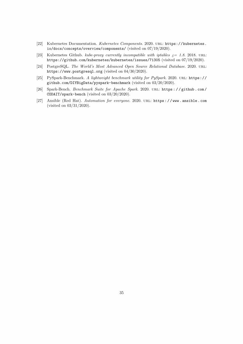
By decreasing the number of entries (Figure 25) we observe a non-linear decay indicatingthat the amount of memory available on the Pi may be a bottleneck.

26

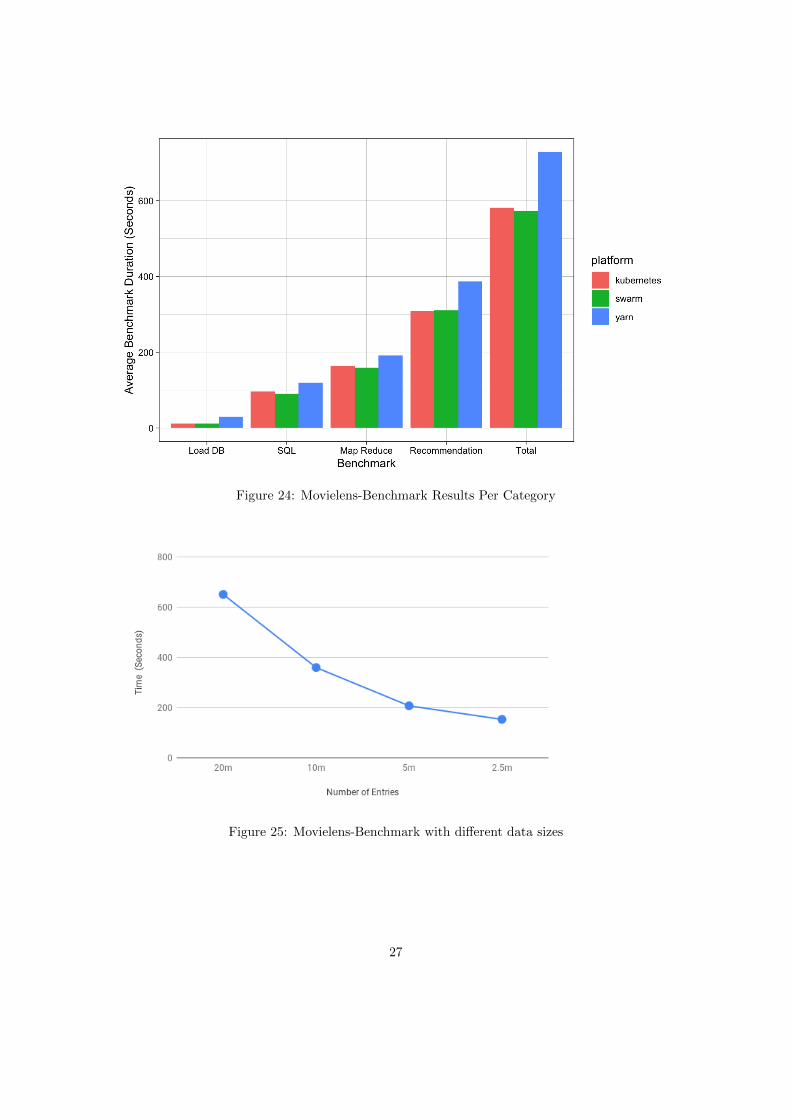
Figure 24: Movielens-Benchmark Results Per Category

Figure 25: Movielens-Benchmark with different data sizes

27

4.3 32bit vs 64bit

The RaspberryPi 4 has a 64-bit processor, but thus far we were running a 32-bit operatingsystem so we decided to see how the two compare to each other. In theory, we do not expect anyperformance gain since the Pi has a maximum of 4GB (the maximum that 32-bit can handle).To investigated the effect of using a 64-bit over 32-bit architecture, we re-ran the PySparkBenchmarks of chapter 4.1 for one worker and found that the 64-bit architecture performedmarginally faster at 13.9% (see Figure 26). However, the 64bit did perform slower for two testsnamely Calculate Pi and Group By (see Figure 27). So, if there is a choice between 32 and 64bit, then the 64-bit option would be the better choice. However, as of writing, Raspbian has notyet released their 64-bit OS. For now, an Ubuntu 64bit image would have to be used.

Figure 26: PySpark-Benchmark 32 vs. 64 bit Overall

Figure 27: PySpark-Benchmark 32 vs. 64 bit Categories

28

4.4 Database Cluster

To evaluate the performance of the database cluster, we have used PgBench, an integratedbenchmarking tool for PostgreSQL. It runs the same queries (SELECT, UPDATE, INSERT)over and over again to measure the resulting transactions per second. [24] To keep the results asconsistent as possible, all tests were conducted with Docker containers which were destroyed aftereach benchmark run. The clusters itself consists of one PostgreSQL master, three PostgreSQLslaves and one PgBench container. The benchmarks were conducted on 1000000 rows with 8/80client connections and 4 threads available. Each benchmark ran for 30 minutes. The results canbe found in Figure 28.

Figure 28: Database Cluster PgBench Benchmark Results

The baseline is a single PostgreSQL Docker container (fig. 28: far left). For comparison,a Macbook Pro 2018 can reach about 2000 TPS Read-Write and 22000 TPS Read-Only. Tomeasure the overhead of the container orchestration software Swarm (Figure 28: 2nd left), thesame baseline container was deployed in Swarm. The results show that Docker Swarm does havea small overhead especially in read-only tasks. This is probably due to a networking overhead(overlay network and load balancer). However, the differences are marginal which is why we haveused Swarm for the remaining benchmarks.

For the replication cluster, we have used the standard PostgreSQL streaming replication aswell as a more exotic version using Gluster. However, as seen in Figure 28, the write performanceof Gluster is poor. This is because Gluster is primarily a file-system (ideal file-size of 128KB)and not a block-storage [5]. Ceph, a distributed object and block-storage, could be used as analternative. However, distributed file systems are resource intensive (CPU, RAM, Network) andmight not deliver the desired results. The more traditional route for achieving replication iscalled ”streaming replication” and is built into PostgreSQL. However, there is no load balancer

29

nor automatic failover integrated yet (we have used Pgpool II as our load balancer). As seen inFigure 28, the load balancer does have a significant overhead. Nevertheless, the read-performance(all slaves are read-only) increases with the number of client.

To evaluate our sharding performance, we have split the ”pgbench accounts” table into 4partitions. The partitions are either kept local (Figure 28: 2nd right) or distributed and mountedusing the FDW (Figure 28: far right). This approach is not ideal because the pgbench tables areinherently connected, yet, partitioning requires independent tables for optimal results. However,we argue that the benchmark should not be chosen because of the database but because itcovers meaningful test cases. Figure 28 shows that partitioning does have a slight but negligibleimpact on performance. Sharding, on the other hand, shows very poor performance in bothread and write benchmarks. We assume that this is probably due to the small table size andsmall load. For example, a B+ Tree has logarithmic complexity which means the table has tobe extremely large for a noticeable performance impact (e.g. Instagram [18]). For small tablesizes, the overhead (e.g. network) is simply too large.

4.5 Experiments Summary

In this project, we have evaluated the performance of Spark and PostgreSQL on a Raspberry Picluster. For Spark, our findings show that more nodes increase the performance of the clustersub-linearly. Moreover, we found that YARN has a considerable overhead compared to DockerSwarm and Kubernetes. For PostgreSQL, we show that scaling with streaming replication is moreefficient than sharding. However, this only applied to low workloads because the RaspberryPi hardware is not powerful enough to handle and simulate lots of clients. In summary, acluster increases the performance though the hardware is not powerful enough to compete withproduction servers.

Based on our findings, we suggest using Kubernetes or Docker Swarm to manage the Rasp-berry Pi cluster. Kubernetes is considerably more complex than Docker Swarm which is why werecommend Docker Swarm as long as the functionality is sufficient. This should be the case foreducational purposes.

30

5 Designing Exercises

This section covers the challenges and reasoning behind the students’ exercises. The exercisesare divided into four categories. First, the hardware and software of the cluster is setup. Second,services such as JupyterLab and Spark are deployed. Third, Spark is introduced with challengingyet beginner-friendly exercises. Last but not least, the resilience of the cluster is tested bydisconnecting nodes. All exercises are complemented by video tutorials for an optimal learningexperience.

Based on the previous section, we have decided to use Docker Swarm as our primary clustermanagement software because of its simplicity and performance. Furthermore, we use Raspbianas our operating system because it is officially supported and a 64-bit version will be availablesoon (according to their forum [1]).

5.1 Cluster Setup

Setting up and maintaining a RPi cluster can be challenging and time-consuming, especially inan educational environment. For this reason, we have decided to use an automation tool calledAnsible [27]. With Ansible, it is possible to configure and deploy software on multiple servers inparallel. The only requirement is to have Ansible installed on a control node (e.g. laptop) withan ssh connection to all remote hosts (e.g. servers). [27] Figure 29 illustrates the setup.

Figure 29: Ansible Overview

Ansible is based on modules (e.g. shell, apt, docker) that can be executed on the remoteservers. The modules provide built-in checks (e.g. if a software is already installed) to avoidunnecessary executions of commands. Ansible commands can be run can be executed directlyin the shell or stored in an Ansible Playbook. For comparison, an Ansible Playbooks is similarto a bash-script but contains Ansible commands. [27] To give an example, Listing 4 shows howto install Vim (text editor) with the apt-module. The module checks if Vim is already installedand acts accordingly.

31

# Run Ansible (Shell)

ansible all -m apt -a "name=vim state=latest" --become

# Run Ansible (Playbook)

ansible-playbook utilities.yaml

# Content of utilities.yaml

- name: Install Basic Utilities

hosts: all

become: true

tasks:

- name: "Install Vim"

apt: name=vim state=latest

Listing 4: Ansible Example

By providing Ansible Scripts (Playbooks) to the students, we can hide the complexity ofsetting up a cluster, yet, still give them insights into the workflow. For example, it is presumablynot interesting for students to configure Gluster. Managing and automating a cluster, however, isprobably interesting because most courses do not cover such practical problems. As a downside,Ansible and SSH have to be installed on a control node (e.g. students laptop). Furthermore, itis currently not possible to set the hostname without booting the Raspberry Pi which is why ascreen has to be provided for the initial boot [1]. Last but not least, we have decided to fix theDHCP address on the router and not use a static IP. This way, students don’t have to worryconfiguring an IP address but the router has to be configured in advance.

5.2 Service Deployment

Deploying all necessary services could be automated but we have purposefully decided againstit. The goal of the exercises is to give the students an opportunity to work with a cluster whichincludes deploying and managing services. The advantage is that students can try differentparameters such as the number of Spark workers. The primary services running on the clusterare Spark, JupyterLab, and a Visualizer (see Table 8). Spark consists of one master and severalworkers. The workers are replicas which is why they can’t be directly accessed (the same portis published for all replicas). JupyterLab mounts the Docker socket to be able to start servicesfrom within (it has to be restricted to the master because only the master can deploy services).For persistent storage, the Gluster volume is mounted on all services. The Visualizer creates agraphical representation of all running services and has to be mounted on the master as well. Insummary, the following services are deployed:

Service PortVisualizer 80Spark UI 8080

JupyterLab 8888

Table 8: Service Names & Ports

32

5.3 Spark Introduction Exercises

Students should be able to write PySpark code and understand the basic principles of SparkRDD’s and Dataframes. This knowledge is taught in the course ”Big-Data Analytics” andis a prerequisite for testing the resilience as a next step of the exercise part. To enable aquick start, we have included instructions on how to upload an example dataset into the GFSdirectory either manually or via terminal. We have written the instruction on the basis of ourMovielens dataset, which we used for the second benchmark test in chapter 4.2. Since thetime for interactive sessions is limited, we provided a Jupyter Notebook, where students will beable to get familiar with the Movielens Dataset to answer certain questions. These exercisespromote ”Learning by Doing” which means that we guide them through the steps but theyhave to do themselves. Sometimes, this means that they have to use Google, Stackoverflow, orthe PySpark Documentation. Our Jupyter Notebook includes basic operations like reading thedataset, creating summary statistics, joins, and even a few RDD transformations. This shouldalso enable students with little programming experience to get a first understanding of howthe Spark syntax is structured and performed. We also have written a sample solution of theMovielens Jupyter Notebook. So it is possible to simply work through the solutions if the timefor working through the exercises is rather short. This decision is left to the lecturer.

5.4 Testing Resilience

Being able to test the resilience is the main selling point of a Raspberry Pi based cluster. Crashinga node is as simple as disconnecting the power cable. To measure the effect of adding or removingnodes, we provide a template code that parallelizes well. The students are free to use their owncode but a difference in the results should be expected. By measuring how long the code takesto run, it is possible to draw conclusions about the effectiveness of adding or removing nodes.Moreover, a node can be disconnected during a calculation. It should be noted that the clustercrashes when the master is down (restriction of Docker Swarm) or less than two nodes are active(restriction of Gluster).

6 Conclusion & Future Work

In this project, we have successfully setup a Docker Swarm, Kubernetes, and Hadoop YARNcluster on a Raspberry Pi. We have run detailed experiments to compare the performance ofSpark and provided different hypotheses as to why YARN did not perform well. Moreover, wehave setup a PostgreSQL cluster and compared different scaling methods. For possible educa-tional use, we have created practical exercises for students and decided to use Docker Swarmbecause of its simplicity and performance. All exercises include detailed step-by-step instructionsas well as tutorial videos for an optimal learning experience. To simplify the cluster setup processfor the students, we have created automation scripts that hide most of the complexity.

In future work, it will be necessary to switch to a 64-bit version of Raspbian. However, thisonly requires minor changes in the setup e.g. recompiling the Dockerfile. Moreover, a futureversion of Raspbian might include a way to automatically set the hostname without having toboot the device. Such a headless setup would greatly simplify the installation process. In termsof educational value, it would be interesting to see if there is a causal effect of hardware-basedapproaches on students’ performance. This would also include a comparison to purely software-based approaches.

33

References

[1] Raspberry Pi Foundation. Teach, Learn, and Make with Raspberry Pi. 2020. url: https://www.raspberrypi.org (visited on 03/31/2020).

[2] Docker Inc. Securely build and share any application, anywhere. 2020. url: https://www.docker.com (visited on 03/25/2020).

[3] StorageOS. Run stateful applications in Kubernetes. 2020. url: https://storageos.com(visited on 05/02/2020).

[4] Rook. Open-Source, Cloud-Native Storage for Kubernetes. 2020. url: https://rook.io(visited on 05/02/2020).

[5] Gluster Inc. Gluster is a free and open source software scalable network filesystem. 2020.url: https://www.gluster.org (visited on 03/25/2020).

[6] techcrunch. Google takes a step back from running the Kubernetes development infrastruc-ture. 2018. url: https://techcrunch.com/2018/08/29/google-steps-back-from-running-the-kubernetes-infrastructure/ (visited on 07/19/2020).

[7] ditigalocean. An Introduction to Kubernetes. 2015. url: https://www.digitalocean.com/community/tutorials/an-introduction-to-kubernetes (visited on 07/19/2020).

[8] kubernetes. Service Documentation. 2020. url: https://kubernetes.io/docs/concepts/services-networking/service/ (visited on 07/19/2020).

[9] kubernetes. Volume Documentation. 2020. url: https://kubernetes.io/docs/concepts/storage/volumes/ (visited on 07/19/2020).

[10] kubernetes. Namespaces Documentation. 2020. url: https://kubernetes.io/docs/

concepts/overview/working-with-objects/namespaces/ (visited on 07/19/2020).

[11] Marvin. Kubernetes Pod. 2018. url: https://en.wikipedia.org/wiki/Kubernetes#/media/File:Pod-networking.png (visited on 07/19/2020).

[12] Tom While. Hadoop The Definitive Guide. O’Reilly Media, 2012, pp. 45–55.

[13] Shrey Mehrotra Akhil Arora. Learning YARN. O’Reilly Media, 2015.

[14] Sven Helmer. “Spark”. University Lecture. 2020.

[15] Holden Karau et. al. Learning Spark. O’Reilly Media, 2015, pp. 45–55.

[16] Spark. Spark Documentation. 2020. url: http://spark.apache.org/docs/latest/

security.html#configuring-ports-for-network-security (visited on 07/19/2020).

[17] Rick Cattell. “Scalable SQL and NoSQL Data Stores”. In: SIGMOD Rec. 39.4 (May 2011),pp. 12–27. issn: 0163-5808. doi: 10.1145/1978915.1978919. url: https://doi.org/10.1145/1978915.1978919.

[18] Instagram Inc. Sharding and IDs at Instagram. 2012. url: https://instagram-engineering.com/sharding-ids-at-instagram-1cf5a71e5a5c (visited on 04/30/2020).

[19] Kubernetes Documentation. What is Kubernetes? 2020. url: https://kubernetes.io/docs/concepts/overview/what-is-kubernetes/ (visited on 07/19/2020).

[20] Kubernetes Documentation. Creating a single control-plane cluster. 2020. url: https:

//kubernetes.io/docs/setup/production-environment/tools/kubeadm/create-

cluster-kubeadm/ (visited on 07/19/2020).

[21] Platform9. Kubernetes vs Docker Swarm. 2017. url: https://platform9.com/blog/kubernetes-docker-swarm-compared/ (visited on 07/19/2020).

34

[22] Kubernetes Documentation. Kubernetes Components. 2020. url: https://kubernetes.io/docs/concepts/overview/components/ (visited on 07/19/2020).

[23] Kubernetes Github. kube-proxy currently incompatible with iptables ¿= 1.8. 2018. url:https://github.com/kubernetes/kubernetes/issues/71305 (visited on 07/19/2020).

[24] PostgreSQL. The World’s Most Advanced Open Source Relational Database. 2020. url:https://www.postgresql.org (visited on 04/30/2020).

[25] PySpark-Benchmark. A lightweight benchmark utility for PySpark. 2020. url: https://github.com/DIYBigData/pyspark-benchmark (visited on 03/20/2020).

[26] Spark-Bench. Benchmark Suite for Apache Spark. 2020. url: https://github.com/

CODAIT/spark-bench (visited on 03/20/2020).

[27] Ansible (Red Hat). Automation for everyone. 2020. url: https://www.ansible.com

(visited on 03/31/2020).

35

A Cluster Introduction and Setup

36

ReadMe.md 5/28/2020

1 / 5

ExercisesThese exercises are based on the following hostnames and IP addresses. Please adjust them to your specifichardware setup. It is assumed that the IP addresses are fixed e.g. using a router with static DHCP.

Hostname IP Address

cluster1raspberry0 (master/manager) 192.168.2.250

cluster1raspberry1 (slave/worker) 192.168.2.251

cluster1raspberry2 (slave/worker) 192.168.2.252

cluster1raspberry3 (slave/worker) 192.168.2.253

Cluster Setup

First, you have to install Raspbian on all Raspberry Pi e.g. using Etcher. Then, you have to boot the RaspberryPi (with keyboard, monitor), set a unique hostname and enable ssh. It is currently not possible to change thehostname without booting the Raspberry Pi which is why the steps can't be automated.

# open raspi-config sudo raspi-config # change hostname:# 2. Network Options --> N1 Hostname # enable ssh:# 5. Interfacing Options --> P2 SSH # reboot sudo reboot

For automatically setting up the Raspberry Pi cluster with Docker Swarm + GlusterFS, you need Ansible andan ssh connection to all Raspberry Pi. The Ansible scripts together with a short instruction can be foundhere. In summary, you have to change the inventory.ini file to fit your specific hardware setup and run theAnsible scripts as shown below. Please note that the Raspberry Pi is not very robust which means that thescripts can fail (e.g. timeout). If this happens, just re-run the script. In case a Raspberry Pi does not rebootcorrectly (happens often), disconnect/reconnect power and wait for Ansible to finish. Some scripts might takea long time (20 minutes) to finish because the Raspberry Pi is rather slow.

ReadMe.md 5/28/2020

2 / 5

# install utilities such as vim/git ansible-playbook utilities.yaml -i inventory.ini # install Docker ansible-playbook docker.yaml -i inventory.ini # initializes Docker Swarm + GlusterFS ansible-playbook swarm.yaml -i inventory.ini

Service Deployment (Visualizer, Spark, JupyterLab)

To deploy a service on your cluster, you have to use ssh and connect to your master (192.168.2.250) becauseservices can't be deployed on a worker node. First, it is useful to deploy a monitoring tool called Visualizer asshown below. Because of the port mapping (--publish), you can directly access the Visualizer from anybrowser (visit 192.168.2.250:80).

# deploy Visualizer on port 80 and constrain it to the master docker service create --name=viz --publish=80:8080/tcp --constraint=node.role==manager --mount=type=bind,src=/var/run/docker.sock,dst=/var/run/docker.sock alexellis2/visualizer-arm:latest # kill the visualizer if needed docker service rm viz

Now you can deploy Spark with the commands below (detailed instructions here if needed). Adjust theparameters (e.g. --replicas 4) to your needs. The Spark UI can be accessed on port 8080 (visit192.168.2.250:8080).

# create an attachable overlay network# (all spark containers have to be within the same network to be able to connect) docker network create -d overlay --attachable spark

# run spark master# (first run might take about 10 minutes because it has to download the image on all RPi) docker service create --name sparkmaster --network spark --constraint=node.role==manager --publish 8080:8080 --publish 7077:7077 --mount source=gfs,destination=/gfs pgigeruzh/spark:arm bin/spark-class org.apache.spark.deploy.master.Master

ReadMe.md 5/28/2020

3 / 5

# run spark workers# (runs four workers and mounts gluster at /gfs to synchronize files accross all nodes) docker service create --replicas 4 --replicas-max-per-node 1 --name sparkworker --network spark --publish 8081:8081 --mount source=gfs,destination=/gfs pgigeruzh/spark:arm bin/spark-class org.apache.spark.deploy.worker.Worker spark://sparkmaster:7077

Last but not least, you can deploy JupyterLab on port 8888 (visit 192.168.2.250:8888) as shown below.

# run jupyter lab# (constraint to the manager because it mounts the docker socket) docker service create --name jupyterlab --network spark --constraint=node.role==manager --publish 8888:8888 --mount source=gfs,destination=/gfs --mount=type=bind,src=/var/run/docker.sock,dst=/var/run/docker.sock -e SHELL=/bin/bash pgigeruzh/spark:arm jupyter lab --ip=0.0.0.0 --allow-root --NotebookApp.token='' --NotebookApp.password='' --notebook-dir='/gfs'

In summary, you should have the following services up and running.

Service URL

Visualizer 192.168.2.250:80

Spark UI 192.168.2.250:8080

JupyterLab 192.168.2.250:8888

For managing your cluster, the following commands might be useful:

# list all services docker service ls # remove a service docker service rm your-service-name

Introduction to Spark

ReadMe.md 5/28/2020

4 / 5

In this exercise, you will use PySpark and the MovieLens 20M Dataset on movie ratings to answer severalquestions. These exercises promote "Learning by Doing" which means that we guide you through the stepsbut you have to do them yourself. Sometimes, this means that you have to use Google, Stackoverflow, or thePySpark Documentation.

First, visit JupyterLab (192.168.2.250:8888) and upload the MovieLens 20M Dataset into /gfs (default view inthe file explorer). Alternatively, run the following commands in the JupyterLab terminal:

# change directorycd /gfs # install wget apt install wget -y # download and unzip MovieLens dataset wget http://files.grouplens.org/datasets/movielens/ml-20m.zip unzip ml-20m.zip

Now, run this Jupyter Notebook and follow the instructions.

Testing Resilience

For testing the resilience of the cluster, you can try your own code or use the template below. The templatecalculates the mean, standard deviation, min, max, and count of the rating columns and parallelizes well.Other tasks might not parallelize well, hence, they do not profit from additional workers.

import time start_time = time.time() from pyspark.sql import SparkSession if __name__ == "__main__": print("--- start ---") # Connect to the master spark = SparkSession\ .builder\ .master("spark://sparkmaster:7077")\ .appName("resilience") \ .getOrCreate() # Calculate count, mean, sd, min, max of ratings ratings = spark.read.csv('ml-20m/ratings.csv', inferSchema=True, header=True) ratings.describe().show()

ReadMe.md 5/28/2020

5 / 5

# Disconnect spark.stop() print("Duration: %s seconds" % (time.time() - start_time)) print("--- end ---")

First, check JupyterLab, Spark UI, and Visualizer. Make sure that your cluster is in working condition. Afterward,open JupyterLab and create a new notebook. Run the template above (or your own code) and visit Spark UI.Check the number of assigned cores and the duration. If something goes wrong, you can kill the task inSpark UI but make sure to restart the IPython kernel. If everything works as expected, you should see a tablewith descriptive statistics and duration (seconds) in your notebook's output. Remember the duration anddisconnect a worker (or two). Please note that the cluster crashes when master is down or less than twonodes are active. Wait until Spark UI highlights the status of the workers as "DEAD" and re-run thenotebook. Again, check the assigned cores and the duration. The duration should now be longer becauseyou have fewer workers. Last but not least, reconnect the workers, wait till they are "ALIVE" and run thenotebook again. The results should be comparable to the first run.

In a second step, you can try to disconnect the workers while running your notebook. The notebookshould still run to the end but it might take longer because the resources have to be reallocated.

B Spark Exercises

42

Movielens_exercises

May 28, 2020

1 Big Data Analytics with MovieLens DatasetIn this Jupyter Notebook, we will use the MovieLens 20M Dataset on movie ratings to answerseveral tasks by using PySpark. The exercises are structured as a guideline to get familiar with thePyspark syntax. Have also a look on the official pySpark documentation.

Introduction to Movielens dataset

The Introduction exercises have the following goals: - Reading and understanding the schema ofour movielens dataset - Calculating some summary statistics of our dataset - Learn how to performjoins and aggregations using Spark

This will be also illustrated by guided exercises to get a first understanding of Spark - GuidedExercise 1: Which movies are the most popular ones? - Guided Exercise 2: What are the distinctgenres in the Movielens Dataset (RDD)?

Exercises for you: - Exercise 1: Which movies have the highest number of ratings? - Exercise 2:What’s the number of movies in each genre? - Exercise 3: Which movies are a matter of taste?

1.1 Initialize SparksessionExecute the following cell to initialize a Sparksession:

[18]: import pysparkfrom pyspark.sql import SparkSessionspark = SparkSession.builder.master("spark://sparkmaster:7077").↪→appName('movielens').getOrCreate()

1.2 Introduction: Reading the datasetOur movielens dataset contains 20 million ratings and 465’000 tag applications applied to 27’000movies by 138’000 users. It also includs tag genome data with 12 million relevance scores across1100 tags.

The whole dataset contains six CSV files: - genome-scores.csv - genome-tags.csv - links.csv -movies.csv - ratings.csv - tags.csv

In this Introduction exercise, we will have a look on the movies and ratings dataframes.

To read a CSV file in our “ml-20m” folder, we access the DataFrameReader class through readand call the csv() method on it. We also specify option("header", "true") since the first rowof the file contains our column names.

1

[35]: ratings = spark.read.option("header", "true").csv("ml-20m/ratings.csv")ratings.show(5)

+------+-------+------+----------+|userId|movieId|rating| timestamp|+------+-------+------+----------+| 1| 2| 3.5|1112486027|| 1| 29| 3.5|1112484676|| 1| 32| 3.5|1112484819|| 1| 47| 3.5|1112484727|| 1| 50| 3.5|1112484580|+------+-------+------+----------+only showing top 5 rows

Each tuple of the ratings DataFrame represents one rating (rating) for one movie (movieId) byone user (userId). The ratings ranges from 0.5 stars (worst) up to 5.0 stars (best).

We can also have look on the Schema of our dataset (column names and types) by using theprintSchema() method.

[36]: ratings.printSchema()

root|-- userId: string (nullable = true)|-- movieId: string (nullable = true)|-- rating: string (nullable = true)|-- timestamp: string (nullable = true)

Do the same for the movies.csv file. What kind of data is available and how does the schema looklike?

[66]:

+-------+----------------------------------+-------------------------------------------+|movieId|title |genres|+-------+----------------------------------+-------------------------------------------+|1 |Toy Story (1995)|Adventure|Animation|Children|Comedy|Fantasy||2 |Jumanji (1995) |Adventure|Children|Fantasy||3 |Grumpier Old Men (1995) |Comedy|Romance||4 |Waiting to Exhale (1995) |Comedy|Drama|Romance||5 |Father of the Bride Part II (1995)|Comedy

2

|+-------+----------------------------------+-------------------------------------------+only showing top 5 rows

root|-- movieId: string (nullable = true)|-- title: string (nullable = true)|-- genres: string (nullable = true)

1.3 Guided Exercise 1: Which movies are the most popular ones?To get the most popular movies, we are looking for the movies with the highest number of ratings.In this task, we assume the number of ratings as a representative for the most popular movies.To do this, we will perform the following transformations on the ratings DataFrame: - group bymovieId - count the number of users (userId) associated with each movie - rename this column tonum_ratings - sort by num_ratings in descending order

We do these transformations in PySpark and store the DataFrame as most_popular. Have also alook on the official pySpark documentation.

HINT: - Use agg(count()) to perform an aggregate calculation on grouped data. - Don’t forgetthat transformations are lazy in spark. We need to call an action (e.g. show() for Dataframes,take() for RDD’s) explicitly to see the results.

[38]: from pyspark.sql.functions import *

most_popular = ratings.groupBy("movieId").agg(count("userId")).↪→withColumnRenamed("count(userId)", "num_ratings").sort(desc("num_ratings"))

most_popular.show(5)

+-------+-----------+|movieId|num_ratings|+-------+-----------+| 296| 67310|| 356| 66172|| 318| 63366|| 593| 63299|| 480| 59715|+-------+-----------+only showing top 5 rows

Unfortunately, the resulting table only contains movieId and num_ratings. The title of the movieis stored in the movies DataFrame. So, we need an inner join of our most_popular DataFramewith the movies DataFrame on movieId.

3

[67]: most_popular_movies = most_popular.join(movies, most_popular.movieId == movies.↪→movieId)

most_popular_movies.select("title", "num_ratings").show(5, truncate = False)

+--------------------------------+-----------+|title |num_ratings|+--------------------------------+-----------+|Pulp Fiction (1994) |67310 ||Forrest Gump (1994) |66172 ||Shawshank Redemption, The (1994)|63366 ||Silence of the Lambs, The (1991)|63299 ||Jurassic Park (1993) |59715 |+--------------------------------+-----------+only showing top 5 rows

We now have a list of the most popular (or most rated) movies of our movielens dataset. Have youalready watched all of them? :)

1.4 Guided Exercise 2: Understanding RDD (Resilient Distributed Datasets)operations

We will have a look on two core data abstractions of Spark, namely Dataframes and RDD’s.RDDs and DataFrames can be created from external data sources (e.g. HDFS, SQL) or frominternal process steps. Dataframes the are easiest abstraction. One can compare Dataframes witha traditional table with columns and rows, which is generally used for handling workflows withstructured data. If the data is unstructured (has no schema) and the data needs to be manipulatedin non-standard ways, one should use RDD’s. Even though our data is structured, we will use someoperations on RDD’s to understand RDD transformations.

Have a look on the Pyspark Documentation for RDD operations PySpark Package

Execute the following cells and try to understand what map(), flatmap() and take() do

[40]: # Load the data into RDDdata = sc.textFile("ml-20m/movies.csv")

# Split the RDDmoviesRDD = data.map(lambda l: l.split(','))moviesRDD.take(5)

[40]: [['movieId', 'title', 'genres'],['1', 'Toy Story (1995)', 'Adventure|Animation|Children|Comedy|Fantasy'],['2', 'Jumanji (1995)', 'Adventure|Children|Fantasy'],['3', 'Grumpier Old Men (1995)', 'Comedy|Romance'],['4', 'Waiting to Exhale (1995)', 'Comedy|Drama|Romance']]

[41]: # mapReversed = moviesRDD.map(lambda m: m[::-1])

4

Reversed.take(5)

[41]: [['genres', 'title', 'movieId'],['Adventure|Animation|Children|Comedy|Fantasy', 'Toy Story (1995)', '1'],['Adventure|Children|Fantasy', 'Jumanji (1995)', '2'],['Comedy|Romance', 'Grumpier Old Men (1995)', '3'],['Comedy|Drama|Romance', 'Waiting to Exhale (1995)', '4']]

[42]: # flatMapwords = moviesRDD.flatMap(lambda m: list(m))words.take(10)

[42]: ['movieId','title','genres','1','Toy Story (1995)','Adventure|Animation|Children|Comedy|Fantasy','2','Jumanji (1995)','Adventure|Children|Fantasy','3']

1.5 Extracting Distinct Movie GenresNow we will try to combine these operations above by trying to extract all distinct movie genresin our Movielens data. You need to: - Read the csv file located in (“ml-20m/movies.csv”) - Splitthe data and select the corresponding genre column via map() - flatmap() the data –> Remark:Be aware that a movie can contain several genres delimited by ('|') - Print the results bytake()the distinct() genres

[43]: movies_rdd=sc.textFile("ml-20m/movies.csv")

movies_split= movies_rdd.map(lambda lines:lines.split(','))genres=movies_split.map(lambda line:(line[2]))genre=genres.flatMap(lambda l:l.split('|'))genres_distinct=genre.distinct()

print(genres_distinct.take(10))

['Children', 'Fantasy', 'Romance', 'Drama', 'Action', 'Thriller', ' The(1995)"', 'Horror', 'Sci-Fi', 'IMAX']

1.6 Exercise 1: Which movies have the highest ratings (in average)?Now it’s your turn. We want to see which movies are rated to be the best. You need to use theratings DataFrame and:

5

• Group by movieId• Calculate the average rating for each movie and rename this column to avg_rating• Sort by avg_rating in descending order• Join the resulting DataFrame with the movies DataFrame to get the movienames.

NOTE Be sure that you read the movies file

[69]: top_rated =

+-------+-----------+----------+-------+---------------------------------------------------------+-----------+|movieId|num_ratings|avg_rating|movieId|title|genres |+-------+-----------+----------+-------+---------------------------------------------------------+-----------+|108527 |2 |5.0 |108527 |Catastroika (2012)|Documentary||103871 |2 |5.0 |103871 |Consuming Kids: The Commercialization ofChildhood (2008)|Documentary||111548 |1 |5.0 |111548 |Welcome to Australia (1999)|Documentary||95517 |1 |5.0 |95517 |Barchester Chronicles, The (1982)|Drama ||109715 |1 |5.0 |109715 |Inquire Within (2012)|Comedy |+-------+-----------+----------+-------+---------------------------------------------------------+-----------+only showing top 5 rows

You will realize that all of the movies with avg_rating of exactly 5.0 have 2 or less num_ratings .We must investigate the distribution of num_ratings to only consider movies that have a minimumnumber of ratings. Calculate some summary statistics within Spark (consider mean(), min() andmax()) and take a decent value to filter your results:

[47]:

+-------+-----------+-----------------+-------+--------------------+--------------------+|movieId|num_ratings| avg_rating|movieId| title|genres|+-------+-----------+-----------------+-------+--------------------+--------------------+| 318| 63366|4.446990499637029| 318|Shawshank Redempt…|Crime|Drama|| 858| 41355|4.364732196832306| 858|Godfather, The (1…|Crime|Drama|| 50| 47006|4.334372207803259| 50|Usual Suspects,T…|Crime|Mystery|Thr…|

6

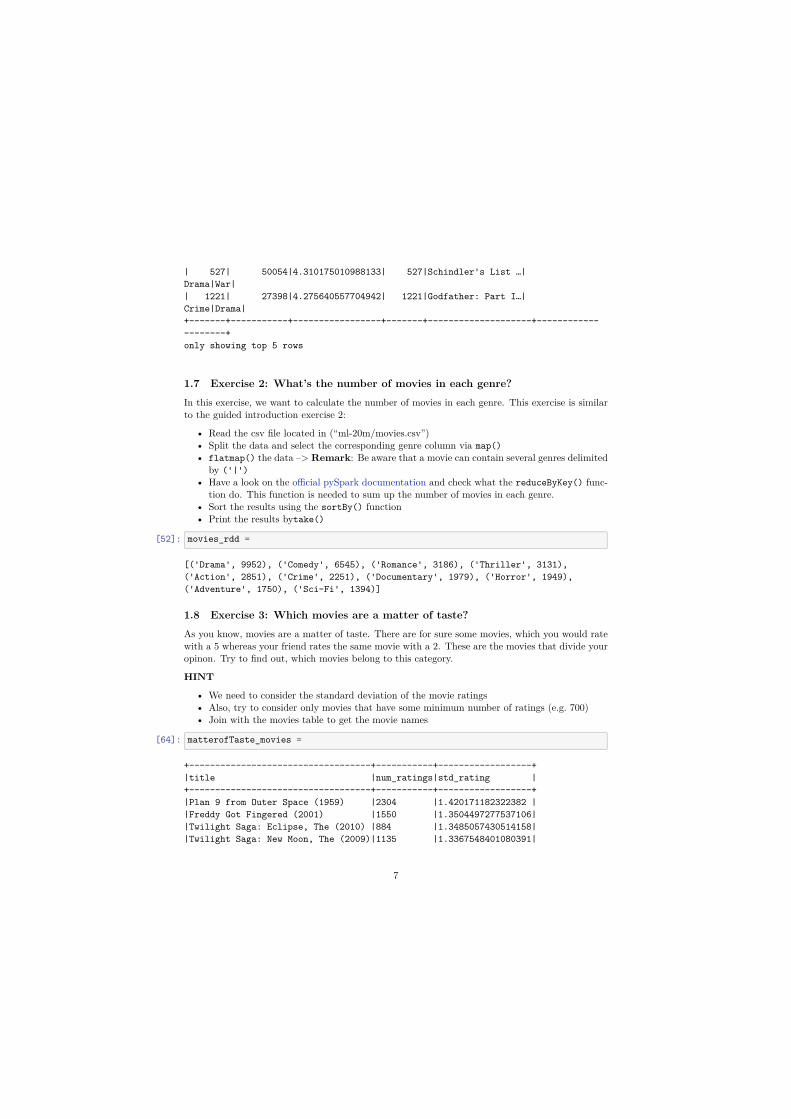
| 527| 50054|4.310175010988133| 527|Schindler's List …|Drama|War|| 1221| 27398|4.275640557704942| 1221|Godfather: Part I…|Crime|Drama|+-------+-----------+-----------------+-------+--------------------+--------------------+only showing top 5 rows

1.7 Exercise 2: What’s the number of movies in each genre?In this exercise, we want to calculate the number of movies in each genre. This exercise is similarto the guided introduction exercise 2:

• Read the csv file located in (“ml-20m/movies.csv”)• Split the data and select the corresponding genre column via map()• flatmap() the data –> Remark: Be aware that a movie can contain several genres delimited

by ('|')• Have a look on the official pySpark documentation and check what the reduceByKey() func-

tion do. This function is needed to sum up the number of movies in each genre.• Sort the results using the sortBy() function• Print the results bytake()

[52]: movies_rdd =

[('Drama', 9952), ('Comedy', 6545), ('Romance', 3186), ('Thriller', 3131),('Action', 2851), ('Crime', 2251), ('Documentary', 1979), ('Horror', 1949),('Adventure', 1750), ('Sci-Fi', 1394)]

1.8 Exercise 3: Which movies are a matter of taste?As you know, movies are a matter of taste. There are for sure some movies, which you would ratewith a 5 whereas your friend rates the same movie with a 2. These are the movies that divide youropinon. Try to find out, which movies belong to this category.

HINT

• We need to consider the standard deviation of the movie ratings• Also, try to consider only movies that have some minimum number of ratings (e.g. 700)• Join with the movies table to get the movie names

[64]: matterofTaste_movies =

+-----------------------------------+-----------+------------------+|title |num_ratings|std_rating |+-----------------------------------+-----------+------------------+|Plan 9 from Outer Space (1959) |2304 |1.420171182322382 ||Freddy Got Fingered (2001) |1550 |1.3504497277537106||Twilight Saga: Eclipse, The (2010) |884 |1.3485057430514158||Twilight Saga: New Moon, The (2009)|1135 |1.3367548401080391|

7