PHY111: Physics I for Physics Majors - UZH - Physik-Institut
158
PHY111: Physics I for Physics Majors PHYSIK INSTITUT UNIVERSITÄT ZÜRICH Prof. Ben Kilminster Fall 2020 Last edited on December 29, 2020 Typeset & figures by Izaak Neutelings
-
Upload
khangminh22 -
Category
Documents
-
view
1 -
download
0
Transcript of PHY111: Physics I for Physics Majors - UZH - Physik-Institut

PHY111:Physics I for Physics Majors
PHYSIK INSTITUTUNIVERSITÄT ZÜRICH
Prof. Ben KilminsterFall 2020
Last edited on December 29, 2020Typeset & figures by Izaak Neutelings

2

Contents
I Mechanics 9
1 Units & Dimensions 111.1 Fundamental definition of units . . . . . . . . . . . . . . . . . . . . . . . . . 11
1.1.1 Time . . . . . . . . . . . . . . . . . . . . . . . . . . . . . . . . . . . . 131.1.2 Distance . . . . . . . . . . . . . . . . . . . . . . . . . . . . . . . . . . 131.1.3 Mass . . . . . . . . . . . . . . . . . . . . . . . . . . . . . . . . . . . . 13
1.2 Dimensional analysis . . . . . . . . . . . . . . . . . . . . . . . . . . . . . . . 14
2 Measurement & Uncertainty 152.1 Statistical uncertainty . . . . . . . . . . . . . . . . . . . . . . . . . . . . . . 152.2 Systematic uncertainty . . . . . . . . . . . . . . . . . . . . . . . . . . . . . . 162.3 Propagation of errors . . . . . . . . . . . . . . . . . . . . . . . . . . . . . . . 162.4 Scientific notation . . . . . . . . . . . . . . . . . . . . . . . . . . . . . . . . 18
3 Vectors & Reference Frames 193.1 Vectors in coordinate systems . . . . . . . . . . . . . . . . . . . . . . . . . . 193.2 Vector length . . . . . . . . . . . . . . . . . . . . . . . . . . . . . . . . . . . 203.3 Vector sum . . . . . . . . . . . . . . . . . . . . . . . . . . . . . . . . . . . . 203.4 Scalar multiplication . . . . . . . . . . . . . . . . . . . . . . . . . . . . . . . 203.5 Scalar product . . . . . . . . . . . . . . . . . . . . . . . . . . . . . . . . . . 213.6 Vector product . . . . . . . . . . . . . . . . . . . . . . . . . . . . . . . . . . 213.7 Reference frames . . . . . . . . . . . . . . . . . . . . . . . . . . . . . . . . . 22
4 Motion in one dimension 254.1 Uniform motion: constant velocity . . . . . . . . . . . . . . . . . . . . . . . 254.2 Uniform acceleration . . . . . . . . . . . . . . . . . . . . . . . . . . . . . . . 26
4.2.1 Positive acceleration . . . . . . . . . . . . . . . . . . . . . . . . . . . 264.2.2 Negative acceleration . . . . . . . . . . . . . . . . . . . . . . . . . . . 27
4.3 Average velocity . . . . . . . . . . . . . . . . . . . . . . . . . . . . . . . . . . 284.3.1 Torricelli’s equation . . . . . . . . . . . . . . . . . . . . . . . . . . . 28
4.4 Instantaneous velocity . . . . . . . . . . . . . . . . . . . . . . . . . . . . . . 294.5 Instantaneous acceleration . . . . . . . . . . . . . . . . . . . . . . . . . . . . 30
5 Motion in two dimensions 355.1 Parabolic motion . . . . . . . . . . . . . . . . . . . . . . . . . . . . . . . . . 36
5.1.1 Example: Shooting a falling monkey . . . . . . . . . . . . . . . . . . 375.2 Interlude: Radians & polar coordinates . . . . . . . . . . . . . . . . . . . . . 385.3 Uniform circular motion . . . . . . . . . . . . . . . . . . . . . . . . . . . . . 405.4 Motion along a general path . . . . . . . . . . . . . . . . . . . . . . . . . . . 43
3

4 CONTENTS
6 Laws of Motion & Forces 456.1 Momentum . . . . . . . . . . . . . . . . . . . . . . . . . . . . . . . . . . . . 456.2 Newton’s laws of motion . . . . . . . . . . . . . . . . . . . . . . . . . . . . . 45
6.2.1 Interlude: Algorithm to solving forces . . . . . . . . . . . . . . . . . 476.3 Gravitational force . . . . . . . . . . . . . . . . . . . . . . . . . . . . . . . . 476.4 Normal force . . . . . . . . . . . . . . . . . . . . . . . . . . . . . . . . . . . 486.5 Springs & Hooke’s law . . . . . . . . . . . . . . . . . . . . . . . . . . . . . . 506.6 Tension . . . . . . . . . . . . . . . . . . . . . . . . . . . . . . . . . . . . . . 50
6.6.1 Example 1: Falling mass . . . . . . . . . . . . . . . . . . . . . . . . . 516.6.2 Example 2: Two masses balancing over pulleys . . . . . . . . . . . . 526.6.3 Example 3: Three unequal masses . . . . . . . . . . . . . . . . . . . 53
6.7 Centripetal force . . . . . . . . . . . . . . . . . . . . . . . . . . . . . . . . . 536.7.1 Example: Mass on a string . . . . . . . . . . . . . . . . . . . . . . . 54
6.8 Friction . . . . . . . . . . . . . . . . . . . . . . . . . . . . . . . . . . . . . . 556.8.1 Example: Friction on an inclined plane . . . . . . . . . . . . . . . . . 566.8.2 Drag . . . . . . . . . . . . . . . . . . . . . . . . . . . . . . . . . . . . 57
7 Work & Energy 597.1 Work . . . . . . . . . . . . . . . . . . . . . . . . . . . . . . . . . . . . . . . . 597.2 Kinetic energy . . . . . . . . . . . . . . . . . . . . . . . . . . . . . . . . . . 60
7.2.1 Example: Lifting a weight . . . . . . . . . . . . . . . . . . . . . . . . 617.2.2 Work integral over a path . . . . . . . . . . . . . . . . . . . . . . . . 61
7.3 Conservative & non-conservative forces . . . . . . . . . . . . . . . . . . . . . 637.3.1 Example 1: Gravity . . . . . . . . . . . . . . . . . . . . . . . . . . . 647.3.2 Example 2: F “ yx` x2x . . . . . . . . . . . . . . . . . . . . . . . . 64
7.4 Potential energy . . . . . . . . . . . . . . . . . . . . . . . . . . . . . . . . . 657.4.1 Gravitational potential energy . . . . . . . . . . . . . . . . . . . . . . 657.4.2 Spring energy . . . . . . . . . . . . . . . . . . . . . . . . . . . . . . . 66
7.5 Energy conservation . . . . . . . . . . . . . . . . . . . . . . . . . . . . . . . 677.5.1 Example 1: Ramp . . . . . . . . . . . . . . . . . . . . . . . . . . . . 677.5.2 Example 2: Pendulum . . . . . . . . . . . . . . . . . . . . . . . . . . 68
7.6 Energy loss due to friction . . . . . . . . . . . . . . . . . . . . . . . . . . . . 687.7 Power . . . . . . . . . . . . . . . . . . . . . . . . . . . . . . . . . . . . . . . 69
8 Conservation of momentum 718.1 Elastic & inelastic collisions . . . . . . . . . . . . . . . . . . . . . . . . . . . 72
8.1.1 Example 1: Two masses colliding elastically in 1D . . . . . . . . . . 738.1.2 Example 2: Two masses colliding inelastically in 1D . . . . . . . . . 748.1.3 Example 3: Walking on ice . . . . . . . . . . . . . . . . . . . . . . . 748.1.4 Example 4: Two masses colliding inelastically in 2D . . . . . . . . . 748.1.5 Example 5: Ballistic pendulum . . . . . . . . . . . . . . . . . . . . . 75
8.2 Impulse . . . . . . . . . . . . . . . . . . . . . . . . . . . . . . . . . . . . . . 768.3 Center of mass . . . . . . . . . . . . . . . . . . . . . . . . . . . . . . . . . . 77
8.3.1 Example: Two mass in 1D . . . . . . . . . . . . . . . . . . . . . . . . 788.4 Inertial frames of reference . . . . . . . . . . . . . . . . . . . . . . . . . . . . 79

CONTENTS 5
9 Torque & Angular momentum 819.1 Torque . . . . . . . . . . . . . . . . . . . . . . . . . . . . . . . . . . . . . . . 819.2 Angular acceleration . . . . . . . . . . . . . . . . . . . . . . . . . . . . . . . 829.3 Rotational equilibrium & moment of inertia . . . . . . . . . . . . . . . . . . 83
9.3.1 Example 1: Balancing two masses on a seesaw . . . . . . . . . . . . . 859.3.2 Example 2: Moment of inertia of two masses . . . . . . . . . . . . . 869.3.3 Example 3: Moment of inertia of a ring . . . . . . . . . . . . . . . . 879.3.4 Example 4: Moment of inertia of a hollow cylinder . . . . . . . . . . 879.3.5 Example 5: Moment of inertia of a solid cylinder . . . . . . . . . . . 889.3.6 Example 6: Moment of inertia of a disk . . . . . . . . . . . . . . . . 889.3.7 Example 7: Moment of inertia of a hollow sphere . . . . . . . . . . . 889.3.8 Example 8: Moment of inertia of a solid sphere . . . . . . . . . . . . 889.3.9 Example 9: Large wheel/disk . . . . . . . . . . . . . . . . . . . . . . 89
9.4 Kinetic energy of rotation . . . . . . . . . . . . . . . . . . . . . . . . . . . . 909.4.1 Example: Large wheel . . . . . . . . . . . . . . . . . . . . . . . . . . 919.4.2 Kinetic energy of a system of particles . . . . . . . . . . . . . . . . . 91
9.5 Parallel axis theorem . . . . . . . . . . . . . . . . . . . . . . . . . . . . . . . 929.5.1 Example 1: Moment of inertia of two masses (revisited) . . . . . . . 939.5.2 Example 2: Moment of inertia of a ring (revisited) . . . . . . . . . . 93
9.6 Angular momentum . . . . . . . . . . . . . . . . . . . . . . . . . . . . . . . 939.6.1 Conservation of angular momentum . . . . . . . . . . . . . . . . . . 95
9.7 Precession . . . . . . . . . . . . . . . . . . . . . . . . . . . . . . . . . . . . . 969.8 Rolling . . . . . . . . . . . . . . . . . . . . . . . . . . . . . . . . . . . . . . . 97
9.8.1 Example: Rolling off a ramp . . . . . . . . . . . . . . . . . . . . . . 989.9 Stability . . . . . . . . . . . . . . . . . . . . . . . . . . . . . . . . . . . . . . 98
9.9.1 Example 1: Ladder . . . . . . . . . . . . . . . . . . . . . . . . . . . . 1009.9.2 Example 2: Rectangular block . . . . . . . . . . . . . . . . . . . . . 1019.9.3 Example 3: Tightrope artist . . . . . . . . . . . . . . . . . . . . . . . 102
9.10 Summary . . . . . . . . . . . . . . . . . . . . . . . . . . . . . . . . . . . . . 102
10 Non-inertial reference frames & Pseudo Forces 10510.1 Inertial reference frames . . . . . . . . . . . . . . . . . . . . . . . . . . . . . 10510.2 Non-inertial reference frames . . . . . . . . . . . . . . . . . . . . . . . . . . 106
10.2.1 Coordinate transformation . . . . . . . . . . . . . . . . . . . . . . . . 10710.3 Rotational frames . . . . . . . . . . . . . . . . . . . . . . . . . . . . . . . . . 108
10.3.1 Centrifugal force . . . . . . . . . . . . . . . . . . . . . . . . . . . . . 10810.3.2 Extra: Coordinate transformation of rotation . . . . . . . . . . . . . 10810.3.3 Extra: Time derivation of a vector function . . . . . . . . . . . . . . 11010.3.4 Pseudo forces in a rotating system . . . . . . . . . . . . . . . . . . . 11110.3.5 Coriolis force . . . . . . . . . . . . . . . . . . . . . . . . . . . . . . . 11210.3.6 Example: Throwing a ball on rotating disk . . . . . . . . . . . . . . 11310.3.7 Example: A ball at rest . . . . . . . . . . . . . . . . . . . . . . . . . 11410.3.8 Example: Centrigufal force on Earth . . . . . . . . . . . . . . . . . . 11410.3.9 Example: Coriolis force on Earth . . . . . . . . . . . . . . . . . . . . 115
II Oscillations and Waves 117
11 Harmonic oscillations 11911.1 Interlude: Taylor expansion . . . . . . . . . . . . . . . . . . . . . . . . . . . 119

6 CONTENTS
11.1.1 Example 1: Cubic function . . . . . . . . . . . . . . . . . . . . . . . 11911.1.2 Example 2: Sine . . . . . . . . . . . . . . . . . . . . . . . . . . . . . 12011.1.3 Example 3: Cosine . . . . . . . . . . . . . . . . . . . . . . . . . . . . 121
11.2 Simple harmonic oscillator . . . . . . . . . . . . . . . . . . . . . . . . . . . . 12111.2.1 Initial conditions . . . . . . . . . . . . . . . . . . . . . . . . . . . . . 12311.2.2 General solution . . . . . . . . . . . . . . . . . . . . . . . . . . . . . 12411.2.3 Energy of a harmonic oscillator . . . . . . . . . . . . . . . . . . . . . 12411.2.4 Vertical harmonic oscillator . . . . . . . . . . . . . . . . . . . . . . . 12511.2.5 Double spring . . . . . . . . . . . . . . . . . . . . . . . . . . . . . . . 126
11.3 Pendulum . . . . . . . . . . . . . . . . . . . . . . . . . . . . . . . . . . . . . 12611.3.1 Physical pendulum . . . . . . . . . . . . . . . . . . . . . . . . . . . . 128
11.4 Damped harmonic oscillators . . . . . . . . . . . . . . . . . . . . . . . . . . 12911.4.1 Energy loss . . . . . . . . . . . . . . . . . . . . . . . . . . . . . . . . 12911.4.2 Quality factor . . . . . . . . . . . . . . . . . . . . . . . . . . . . . . . 13011.4.3 Underdamping . . . . . . . . . . . . . . . . . . . . . . . . . . . . . . 13111.4.4 Critical damping and overdamping . . . . . . . . . . . . . . . . . . . 13211.4.5 Energy (revisited) . . . . . . . . . . . . . . . . . . . . . . . . . . . . 132
11.5 Driven oscillation & resonance . . . . . . . . . . . . . . . . . . . . . . . . . . 13311.5.1 Real-life examples . . . . . . . . . . . . . . . . . . . . . . . . . . . . 134
12 Hydrostatics & Pressure 13712.1 Atmospheric pressure . . . . . . . . . . . . . . . . . . . . . . . . . . . . . . . 13712.2 Microscopic description . . . . . . . . . . . . . . . . . . . . . . . . . . . . . 13812.3 Bulk modulus . . . . . . . . . . . . . . . . . . . . . . . . . . . . . . . . . . . 13912.4 Pressure variation with depth . . . . . . . . . . . . . . . . . . . . . . . . . . 139
12.4.1 Air pressure variation with altitude and weather . . . . . . . . . . . 14112.5 Measuring pressure . . . . . . . . . . . . . . . . . . . . . . . . . . . . . . . . 141
12.5.1 Manometer . . . . . . . . . . . . . . . . . . . . . . . . . . . . . . . . 14112.5.2 Barometer . . . . . . . . . . . . . . . . . . . . . . . . . . . . . . . . . 14212.5.3 Torricelli’s experiment . . . . . . . . . . . . . . . . . . . . . . . . . . 14212.5.4 Drinking from a long straw . . . . . . . . . . . . . . . . . . . . . . . 143
12.6 Pascal’s principle . . . . . . . . . . . . . . . . . . . . . . . . . . . . . . . . . 14312.7 Buoyancy . . . . . . . . . . . . . . . . . . . . . . . . . . . . . . . . . . . . . 144
12.7.1 Archimedes’ principle . . . . . . . . . . . . . . . . . . . . . . . . . . 14512.7.2 Example: Iceberg . . . . . . . . . . . . . . . . . . . . . . . . . . . . . 14612.7.3 Archimedes’ trick: Measuring density . . . . . . . . . . . . . . . . . . 146
13 Fluids in motion 14913.1 Continuity equation . . . . . . . . . . . . . . . . . . . . . . . . . . . . . . . 14913.2 Bernouilli’s equation . . . . . . . . . . . . . . . . . . . . . . . . . . . . . . . 150
13.2.1 Torricelli’s law . . . . . . . . . . . . . . . . . . . . . . . . . . . . . . 15113.2.2 Venturi effect . . . . . . . . . . . . . . . . . . . . . . . . . . . . . . . 152
13.3 Current resistance & viscous flow . . . . . . . . . . . . . . . . . . . . . . . . 15213.4 Laminar & turbulent flow . . . . . . . . . . . . . . . . . . . . . . . . . . . . 15313.5 Magnus effect . . . . . . . . . . . . . . . . . . . . . . . . . . . . . . . . . . . 154
14 Surface tension 15714.1 Surfactants & soap bubbles . . . . . . . . . . . . . . . . . . . . . . . . . . . 15814.2 Capillary action . . . . . . . . . . . . . . . . . . . . . . . . . . . . . . . . . . 158

Introduction
Physics! What exactly is it and what is it useful for? Physics deals with matter, energy,the principles of motion for particles and waves, and their interactions. It aims to explainproperties and behavior of things at the small level, such as molecules, atoms, nuclei andquarks; but also at the larger scale, such as gases, liquids, solids, but also plants, stars,solar systems and star clusters. Physics is the study of the fundamental laws of nature, andis necessary to understand chemistry, biology, astronomy, cosmology, etc. at a fundamentallevel. If you want to understand the basics of how things work, this is the place to be!
These lecture notes cover the basics of classical mechanics for first-year physics students.We will starts off with some basic concepts like units and dimension and how to describemotion with kinematics. After that, we will learn about the Newtonian laws that governmotion using forces. Then we will discuss fluid dynamics, and finally finish off with thestudy of waves mechanics.
A good reference and source of materials for the topics discussed here can be found inPart I of Fundamentals of Physics by David Halliday, Robert Resnick & Jearl Walker. Itcontains many more examples and exercises. This book is available in both English andGerman.
In case you find any errors or typos, please send an e-mail to [email protected] [email protected].
7

8 CONTENTS

Part I
Mechanics
9


Chapter 1
Units & Dimensions
Before we can start uncovering the underlying principles of Nature we need to understandthe basic ingredients.
1.1 Fundamental definition of units
The basic units that are used in science are defined by the International System of Units(SI). The system has seven basic units for seven quantities, or dimensions:
• seconds (s) for time,
• meter (m) for distance or length,
• kilogram (g) for mass,
• Ampere (A) for electrical current,
• Kelvin (K) for temperature,
• mole (mol) for amount of substance, and
• candela (C) for luminous intensity.
This semester, we will focus only on time, distance and mass.From all of these units, we can derive any other unit we need in physics. Table 1.1
contains some of examples of derived units we need this semester. Table 1.2 lists the officialprefixes in the SI unit system.
Note that the choice of these seven dimensions and their units are in some sense arbi-trary. Alien scientists on another planets might have chosen a different set of dimensionsor units to base their alien physics on, although we still expect the laws of physics to bethe same.
However, the definition of units needs to be rigorously standardized for scientific, tech-nological, and financial reasons (such as trade). Before the world was as interconnectedas is today, each village could have its own definition for length, mass or time. They wereoften based on the (average) length of some body part, like feet, hands or forearms. Be-sides the fact that the average foot length could be larger one village over, how can youconvert between these? How many elbows are there in a feet? At some point, people triedto fix units more widely with some standards. In case of the metric system, on which theSI units are based, this came about after the French Revolution. These standards wouldbe some artefact, or prototype. It could be a bar that set the definition of the meter, or a
11
12 CHAPTER 1. UNITS & DIMENSIONS
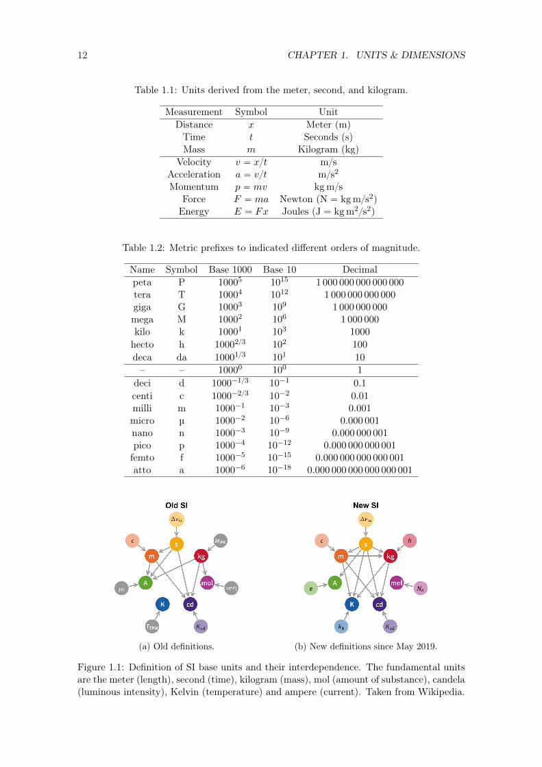
Table 1.1: Units derived from the meter, second, and kilogram.
Measurement Symbol UnitDistance x Meter (m)Time t Seconds (s)Mass m Kilogram (kg)
Velocity v “ x{t m{sAcceleration a “ v{t m{s2
Momentum p “ mv kg m{sForce F “ ma Newton (N “ kg m{s2)Energy E “ Fx Joules (J “ kg m2{s2)
Table 1.2: Metric prefixes to indicated different orders of magnitude.
Name Symbol Base 1000 Base 10 Decimalpeta P 10005 1015 1 000 000 000 000 000tera T 10004 1012 1 000 000 000 000giga G 10003 109 1 000 000 000mega M 10002 106 1 000 000kilo k 10001 103 1000
hecto h 10002{3 102 100
deca da 10001{3 101 10
– – 10000 100 1
deci d 1000´1{3 10´1 0.1
centi c 1000´2{3 10´2 0.01milli m 1000´1 10´3 0.001micro µ 1000´2 10´6 0.000 001nano n 1000´3 10´9 0.000 000 001pico p 1000´4 10´12 0.000 000 000 001femto f 1000´5 10´15 0.000 000 000 000 001atto a 1000´6 10´18 0.000 000 000 000 000 001
(a) Old definitions. (b) New definitions since May 2019.
Figure 1.1: Definition of SI base units and their interdependence. The fundamental unitsare the meter (length), second (time), kilogram (mass), mol (amount of substance), candela(luminous intensity), Kelvin (temperature) and ampere (current). Taken from Wikipedia.

1.1. FUNDAMENTAL DEFINITION OF UNITS 13
block of weight that set the kilogram. These would be securely stored in Paris, and otherinstitutes could request a copy. However, over time this method proved unreliable.
A new approach was chosen, which took effect as of May of 2019. The base units of theSI system are now all defined to depend on the measurements of fundamental constants,which have been fixed to one value for ever. Figure Fig. 1.1 summarizes the definition ofthe base units with constants of Nature and their interdependence. We will look at someexamples below.
1.1.1 Time
Time used to be defined by the orbit of the earth around the sun. Now, however, we usea more precise atomic clock. This “clock” is based on the transition rate of Cesium-133atoms. When a liquid of Cesium isotopes is heated up inside an oven, it will emit a beamof Cesium atoms in either of two states. A microwave cavity is precisely tuned to switchbetween these two states based on the natural oscillation frequency of the Cesium, andmagnets are used to select one of these states, such that when the frequency is perfectlymatched, we get a Cesium beam which is maximally detected as being in one of these states.Therefore a second is defined exactly as the time it takes for 9 192 631 770 oscillations ofthe microwaves in the cavity. The relative precision of such an atomic clock is typically
∆T
T„
1 s
100 My, (1.1)
so 1 second in 100 million years.
1.1.2 Distance
The meter was defined such that distance from the equator through Paris to the north polewould be 107 meters. The circumference of the earth is about 40 000 km. Now, the meteris defined using the definition of the speed of light, c, and the definition of the seconds.One meter is defined as exactly the distance light travels in
1
299 792 458seconds, (1.2)
such thatc “ 299 792 458 m{s. (1.3)
1.1.3 Mass
The kilogram used to be defined by a standard object, which was a metal object keptunder vacuum in a vault in Paris. Since May of 2019, it is defined using Planck’s constanth. This constant relates time and energy via
h “ 6.626 070 15ˆ 10´34 Js. (1.4)
In a later physics course, you will determine h from Einstein’s equation for the energy Eof a photon with frequency ν,
E “ hν. (1.5)
The kilogram then, is defined by seconds (from the Cesium clock), meters (from c), andJoules (from h).

14 CHAPTER 1. UNITS & DIMENSIONS
1.2 Dimensional analysis
We know we cannot add seconds to meters, as they have different dimensions, time andlength, respectively. What about
x “E
F` vt`
a
v, (1.6)
with distance x, energy E, force F , velocity v, time t and acceleration a? Is this a validequation? From Table 1.1, we know that the units of the first term on the right-hand sideis
„
E
F
“rEs
rF s“
kg m2{s2
kg m{s2 , (1.7)
while the second term isrvts “ m{s ¨ s “ m, (1.8)
and the third term,”a
v
ı
“ras
rvs“
m{s2
m{s“
1
s. (1.9)
Each term in Eq. (1.6) has different units, so the equation cannot possibly be valid.This check is called dimensional analysis. Its one of the most powerful tools at the
disposal of a physicist. If you came to a final results after a lot of algebra, it is one way totest if you made any mistakes along the way. It can also be useful to remember formulas.In fact, dimensional analysis is even used to guess the form of some unknown equationas ansatz, if one knows what the possible ingredients (i.e. the possible variables) andrestrictions of your problem are.

Chapter 2
Measurement & Uncertainty
Let’s say we want to measure some distance x. To get a more precise value, it’s oftenbetter to make the measurement several times and take the average:
x “1
n
nÿ
i“1
xi, (2.1)
where xi are n measurements of x. This is our data set. The average is sometimes as theexpected value xxy “ x of x, written with brackets.
However, measurements in science are meaningless without some estimate of the un-certainty, or error, on the result. They are typically denoted with σ. There are two typeof uncertainties that we will see now.
2.1 Statistical uncertainty
In statistics, we typically look at how spread out our data set is. If the real value is x, thatthe standard deviation is defined as
σ “1
n
g
f
f
e
nÿ
i
px´ xiq2. (2.2)
However, we don’t know the true value of x, since this is exactly what we are trying tomeasure. So instead we substitute the average, and the formula becomes
Standard deviation.
σ “
g
f
f
e
1
n´ 1
nÿ
i
px´ xiq2, (2.3)
such that for n Ñ 8, these two definitions are the same. This number gives you an ideaof the “spread”, or variance, of your measurements.
We can also estimate what the uncertainty in our measurement of the average xis:
15

16 CHAPTER 2. MEASUREMENT & UNCERTAINTY
Measurement error.
σx “σ?n“
g
f
f
e
1
npn´ 1q
nÿ
i
px´ xiq2. (2.4)
This is our measurement error or statistical error in our measurement of x. It is also calledthe standard error of the mean. Again, as our data set increases, our uncertainty becomessmaller.
Example 2.1: Consider the data set of measurements
t21.4, 21.0, 20.9, 21.3, 21.0, 21.3, 21.2, 21.0u. (2.5)
The average is x “ 21.14, the standard deviation of the data set is σ “ 0.18 and theuncertainty in, or standard error on, x is σx “ 0.07.
This will be covered in a bit more detail in the physics practicum (PHY112).
2.2 Systematic uncertainty
The systematic uncertainty is related to the limited knowledge you have of your measure-ment instruments. As a rule of thumb, this uncertainty is often estimated as the smallestunit of measurement. This is your precision. For example, the precision of most highschool rulers is σx “ 1 mm, because this is the unit of the smallest lines can read off.
However, most instruments can also have some unknown “shift” from the real valuecalled the bias, and need to be properly calibrated, after which the systematic uncertaintyis estimated. This is referred to as the accuracy of your instrument.
2.3 Propagation of errors
In class we measured the speed of light by measuring the time t light travels over a distancex. The speed of light then, simply is
c “x
t. (2.6)
We have estimate the precision as σt “ 2 ns and σx “ 0.01 m, and now we want to estimatethe uncertainty σc in our result c.
In general, if f “ fpx, y, z, ...q, the uncertainty on the quantity f is given by “propa-gating” the uncertainties of its arguments
Propagation of errors.
σf “
d
σx2pBf
Bxq
2
` σy2pBf
Byq
2
` σz2pBf
Bzq
2
` ... (2.7)
Here, B is sometimes called the del symbol. It means that you take derivatives of thefunction f with respect to only of of its variables. The partial derivative
Bf
Bx(2.8)
2.3. PROPAGATION OF ERRORS 17
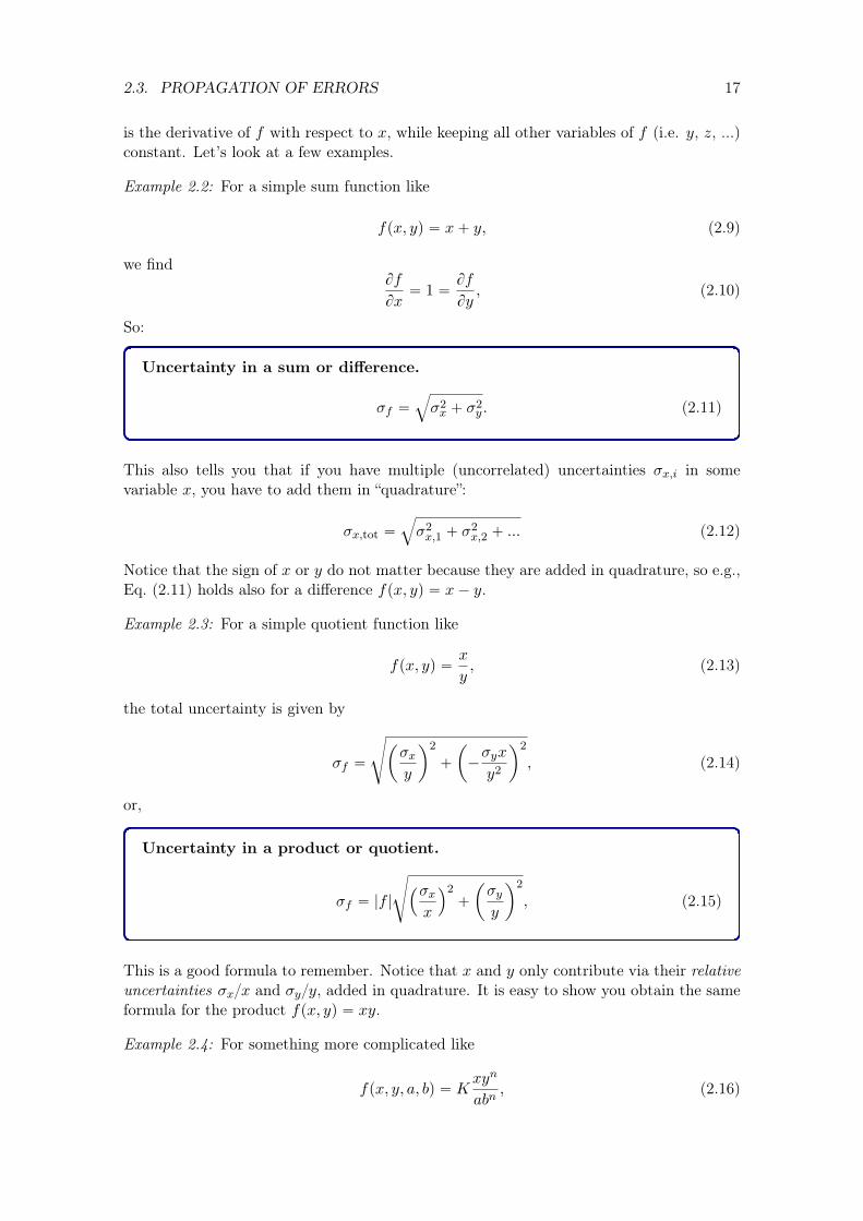
is the derivative of f with respect to x, while keeping all other variables of f (i.e. y, z, ...)constant. Let’s look at a few examples.
Example 2.2: For a simple sum function like
fpx, yq “ x` y, (2.9)
we findBf
Bx“ 1 “
Bf
By, (2.10)
So:
Uncertainty in a sum or difference.
σf “b
σ2x ` σ
2y . (2.11)
This also tells you that if you have multiple (uncorrelated) uncertainties σx,i in somevariable x, you have to add them in “quadrature”:
σx,tot “
b
σ2x,1 ` σ
2x,2 ` ... (2.12)
Notice that the sign of x or y do not matter because they are added in quadrature, so e.g.,Eq. (2.11) holds also for a difference fpx, yq “ x´ y.
Example 2.3: For a simple quotient function like
fpx, yq “x
y, (2.13)
the total uncertainty is given by
σf “
d
ˆ
σxy
˙2
`
ˆ
´σyx
y2
˙2
, (2.14)
or,
Uncertainty in a product or quotient.
σf “ |f |d
´σxx
¯2`
ˆ
σyy
˙2
, (2.15)
This is a good formula to remember. Notice that x and y only contribute via their relativeuncertainties σx{x and σy{y, added in quadrature. It is easy to show you obtain the sameformula for the product fpx, yq “ xy.
Example 2.4: For something more complicated like
fpx, y, a, bq “ Kxyn
abn, (2.16)

18 CHAPTER 2. MEASUREMENT & UNCERTAINTY
with a constant K, we find after some algebra
σf “ |f |d
´σxx
¯2`
ˆ
σyy
˙2
`
´nσaa
¯2`
´nσbb
¯2, (2.17)
which is left as an excellent exercise for home. Notice that the relative uncertainty of yand b contribute more to the overall uncertainty, as they have an extra factor n.
Example 2.5: In our measurement of the speed of light in class, we estimated σx “ 0.01 mto be the uncertainty in the distance x, and σt “ 2 ns in the travel time of light accordingto our oscilloscope. The uncertainty in our measurement of c is
σc “ c
c
´σxx
¯2`
´σtt
¯2“ 0.06. (2.18)
2.4 Scientific notation
If you would measure the height of a A4 paper sheet with a simple high school rulers, youcould write your result for example as
h “ 29.8˘ 0.1 cm.
Here, the three digits (2, 9 and 8) are your significant digits. The uncertainty is alwayswritten with just one significant digit (the zeros in front do not count). Typically you writeonly as many significant digits as your precision. This includes any trailing zeros, e.g. forthe A4 width:
w “ 21.0˘ 0.1 cm.
In science, results are often written in terms of powers of ten. This allows you to keepeasier track of the order of magnitude of your results. For example, for our measurementof c in class:
c “ p2.98˘ 0.06q ˆ 108 m
s.
On calculators the power of ten can be written as 2.98e8. Notice that the power dependson your choice of units; for our A4 sheet:
h “ p2.98˘ 0.01q ˆ 101 cm “ p2.98˘ 0.01q ˆ 10´1 m,
w “ p2.10˘ 0.01q ˆ 101 cm “ p2.10˘ 0.01q ˆ 10´1 m,
because 1 cm “ 1ˆ 10´2 m.In the exercises on the homeworks and exams, it is often sufficient to write down only
three significant digits if you have no uncertainty given.

Chapter 3
Vectors & Reference Frames
Vectors are representations of a quantity that has a certain direction and magnitude. Theyare very useful for a couple of things: to indicate, for example, the velocity of an object(v), or a force acting upon it (F), but also its position with respect to some point (r), oreven differences like displacement (∆r) or change in velocity (∆v). Vectors are typicallyindicated with an arrow, but in these notes, we will use the bold notation.
3.1 Vectors in coordinate systems
The location of an object can be described by a point P in 3D space. In a Cartesiancoordinate system, P has some coordinates px, y, zq, as in Fig. 3.1a. This can also bewritten as a vector r. Using unit vectors x, y and z that point in each of the threedirections:
r “ xx` yy ` zz. (3.1)
Some books also use the convention
r “ xi` yj` zk,
or evenr “ xex ` yey ` zez.
In two dimension, r “ xx` yy, and we simply ignore the z component.
x
y
z
x
yz
Pθ
(a) Position vector in a 3D Cartesiancoordinate system.
(x, y)
r
x
y θ
x = r cos θ
y = r sin θ
(b) Position vector in a 2D Cartesiancoordinate system.
r
xx
yy
x
y
(c) A vector can be broken down intoits x and y vector components.
Figure 3.1: Postition vectors in two dimensions.
19

20 CHAPTER 3. VECTORS & REFERENCE FRAMES
3.2 Vector length
The length, also called the magnitude or modulus, of a vector is given by Pythagoras:
|a| “ a “b
a2x ` a
2y ` a
2z. (3.2)
Note some books use double bars notation. Unit vector have by definition length 1,
|x| “ 1. (3.3)
If you have some vector a, you can normalize it to get its unit vector, written with a pointyhat.
a “a
|a| . (3.4)
A hat (circumflex) always means the vector is normalized to 1.
3.3 Vector sum
Vector summing is very simple: you simply add them component-wise:
a` b “ paxx` ayy ` azzq ` pbxx` byy ` bzzq
“ pax ` bxqx` pay ` byqy ` pay ` byqz.
(3.5)(3.6)
This is shown visually in Fig. 3.2a with the so-called tip-to-tail method. Figure 3.2a showsthe same method for many vectors.
3.4 Scalar multiplication
Vectors can be multiplied by a scalar, or in other words, scaled by a real number b P R:
ba “ baxx` bayy ` bazz. (3.7)
So each component is scaled by the same number. It is easy to show that the length of thenew vector is simple |ba| “ |b|a. This is the main effect: The length changes, but the newvector ba will be parallel to a (if b ‰ 0), like in Fig. 3.3a. In case b ă 0, it will “flip” thedirection. A special case of this is where b “ ´1, such that
´a “ ´axx´ ayy ´ azz, (3.8)
which means that ´a is parallel to a, has the same length, but points in the oppositedirection.
a
b
a
b
a+ b
(a) Summing two vectors.
a
bc
d
(b) A bunch of vectors.
a
b
c
d
a+ b+ c+ d
(c) Tip-to-tail method.
Figure 3.2: Adding vectors.

3.5. SCALAR PRODUCT 21
a
−a
2a
(a) Scalar multiplication ba of vector a withscalar b, where b “ 2 or ´1.
a
a · x = |a| cos θxx
θ
(b) Scalar product x “ r ¨ x is the projection ofr onto the x axis.
Figure 3.3: Multiplication of vectors.
3.5 Scalar product
The scalar product, or dot product, is the componentwise product of two vectors:
a ¨ b “ paxx` ayy ` azzq ¨ pbxx` byy ` bzzq
“ paxbxqx` paybyqy ` pazbzqz.
(3.9)(3.10)
The result is a real number, as opposed to a vector again. Hence the name “scalar”. Aconvenient relation is
a ¨ b “ |a||b| cos θ “ ab cos θ, (3.11)
where θ is the angle between a and b. From either of these formulas, it is trivial to showthat the scalar product is commutative, i.e. swapping two vectors gives the same result:
a ¨ b “ b ¨ a. (3.12)
The scalar product is also distributive with vector sum, which means that for any threevectors a, b and c,
a ¨ pb` cq “ a ¨ b` a ¨ c. (3.13)
Notice that a scalar product of a vector with itself gives you its magnitude squared,
a ¨ a “ |a|2. (3.14)
The scalar product is also useful to codify projection onto some direction given by aunit vector, e.g.
a ¨ x “ a cos θ, (3.15)
where θ is the angle between the x axis and a, as in Fig. 3.3b. So this projection gives youits x component.
Since the y and x axes are orthogonal, or normal, to each other, the y unit vector hasno component along vux and x ¨ y “ 0. This holds for any two vectors that are orthogonalto each other. A different way to see this is by realizing the angle between them is θ “ 90˝,and so cos θ “ 0.
3.6 Vector product
Lastly, there is the vector product, or cross product defined as
aˆ b “ paybz ´ azbyqx` pazbx ´ axbzqy ` paxby ´ aybxqz. (3.16)

22 CHAPTER 3. VECTORS & REFERENCE FRAMES
a× b
a
b θ
(a) The right-hand rule gives the direction of thevector product.
x
y
z
(b) Conventionally, we use a right-handed coor-dinate system.
Figure 3.4: Right-hand rule like on the CHF 200 bill: Point your flat hand in the directionof the first vector a. Keeping your index finger along a, point your middle finger along b,sweeping the smallest angle θ between a and b. Your thumb will point along aˆ b.
One way of remembering this formula is by creating the following matrix, of which youcompute the discriminant:
aˆ b “
∣∣∣∣∣∣
x y zax ay azbx by bz
∣∣∣∣∣∣. (3.17)
This result of the vector product is again a vector, hence the name. The length of thevector products is given by
|aˆ b| “ |a||b| sin θ. (3.18)
This is the vector product’s counterpart of Eq. (3.11).Important to know is that this new vector is orthogonal to the original vectors. It is
easy to show thata ¨ paˆ bq “ 0
b ¨ paˆ bq “ 0.
(3.19)(3.20)
So aˆ a is orthogonal to a and b, but in which direction? There are two possibilities, butthe convention is given by the right-hand rule, illustrated in Fig. 3.4. In fact, the Cartesiancoordinate system we conventionally use in 3D is right handed :
xˆ y “ z. (3.21)
From Eq. (3.18) it is easy to see that the vector product of two non-zero vectors iszero if and only if sin θ “ 0. This happens when they are aligned (θ “ 0) or back-to-back(θ “ 90˝). This also makes sense from a geometrical standpoint, as two aligned vectors donot span a plane anymore, and the vector product has no unique direction to be orthogonalto them. In terms of linear algebra: The two vectors are not linear independent.
Finally, unlike the scalar product, the vector product is not commutative:
aˆ b “ ´bˆ a, (3.22)
but since swapping the vectors only introduces a minus sign, it is called anticommutative.
3.7 Reference frames
We will see many physics problems in the coming chapters and exercise classes. Oneimportant thing is that the choice of the coordinate system is arbitrary. Where you put

3.7. REFERENCE FRAMES 23
xO
y
x′O′
y′
x′′O′′
y′′
x′′′
O′′′
y′′′
Figure 3.5: Different reference frames can describe the same points and vectors, but indifferent coordinates. Several transformations between them or combinations of transfor-mations are possible without changing the physics, like translation, reflection and rotation.The position vector (green) will be different in each frame.
the origin, and in what direction you point the axes is your choice, and the physics (i.e.the prediction) will be the same. That is not to say there are no bad choices. Often thereis a natural choice, such as x for the horizontal direction, along the ground, and y alongthe vertical. The right choice can spare you a lot of extra algebra.
You can do several types of coordinate transformations without changing the physics:
• Translation: px, yq ÞÑ px1, y1q “ px` a, y ` bq.
• Rotation: px, yq ÞÑ px1, y1q “ px cos θ ´ y sin θ, x sin θ ` y cos θq.
• Reflection: px, yq ÞÑ px1, y1q “ px,´yq.
Some of these are illustrated in Fig. 3.5. In theoretical physics this fact is related to thedeeper concept of symmetry : the physics does not change under these transformations,just like rotating a circle by any angle gives you the same shape.
In Chapters 10 we will learn more about inertial and non-inertial reference frames.

24 CHAPTER 3. VECTORS & REFERENCE FRAMES

Chapter 4
Motion in one dimension
Movement can be described by change in coordinates with time. In three dimensions, anobject can move from a point P1 “ px1, y1, z1q to point P2 “ px2, y2, z2q like in Fig. 4.1. Atsome time t1 it was at P1, until it arrived at P2 at some time t2. Its path will be describedby some continuous vector functions
rptq “ xptqx` yptqx` zptqx, (4.1)
where its coordinates x “ xptq, y “ yptq and z “ zptq are again functions of time.In this course we will study the behavior of motion with some relatively simple functions
such as linear, quadratic, circular, and sinusoidal functions.
4.1 Uniform motion: constant velocity
Let’s start with some basic examples in one dimension (1D). If a point is moving in somedimension, it means its position x depends on time t,
x “ xptq. (4.2)
Consider a car driving with a constant velocity v. Its position at any time is then given by
xptq “ vt. (4.3)
This is called uniform linear motion, or uniform motion in one dimension. Fig. 4.2a showthat this look like a straight line through the origin of a position versus time graph. The
x
y
z
r(t1)
P1
r(t2) P2
Figure 4.1: Motion of a point in a 3D. The position vector points to different points alongthe point’s path at different times.
25

26 CHAPTER 4. MOTION IN ONE DIMENSION
t [s]
x [m] x(t) = v0t
t1
x1
t2
x2
(a) Starting at xp0q “ 0 at t “ 0.
t [s]
x [m]x(t) = x0 + v0t
t1 t2x0
x2
(b) Starting at an offset xp0q “ x0 at t “ 0.
Figure 4.2: Uniform motion in one dimension with constant velocity.
slope of the line is the velocity v. For example, between two points pt1, x1q and pt2, x2q,the slope of the line is given by
v “x2 ´ x1
t2 ´ t1“
∆x
∆t. (4.4)
A trivial case is when v “ 0: The point does not move at all in time and it stands still inthe same position. To get a feeling for this: If the car started at xp0q “ 0 at t and movedto xp1 sq “ 5 m after t “ 1 s, the car has an average velocity of 5 m{s.
Note that in Eq. (4.3) we assumed that the car started at xp0q “ 0 at t “ 0. In general,the car could have been at some position xp0q “ x0 at t “ 0, as in Fig. 4.2b:
Uniform motion in one dimension.
xptq “ x0 ` vt. (4.5)
4.2 Uniform acceleration
Velocity of course does not have to be constant. It can depend on time as well:
v “ vptq. (4.6)
For example, if velocity increases with time linearly, starting from some initial velocity v0
thenvptq “ v0 ` at (4.7)
with the constant acceleration a, the position xptq will now become a parabola in x-t space.As velocity has dimensions time over length, acceleration must clearly have dimensionslength over time squared, so units m{s2.
4.2.1 Positive acceleration
Consider again a car which starts from rest (i.e. vp0q “ 0) and speeds up with a constantacceleration, then its position is given by
xptq “ x0 `at2
2, (4.8)
as illustrated in Fig. 4.3a. For simplicity, you could let the car start at xp0q “ x0 “ 0 attime t “ 0. We will understand in a few sections where this equation comes from better.

4.2. UNIFORM ACCELERATION 27
Now consider the car was moving with some initial velocity vp0q “ v0. Its position willbe described by
xptq “ x0 ` v0t`at2
2, (4.9)
instead.
4.2.2 Negative acceleration
Another example is when you throw up a ball. Say we start the clock at t “ 0 when yourelease it from your hand, and count this height as yp0q “ y0 “ 0. The ball will have someinitial velocity vp0q “ v0 that you gave it. At the same time, gravity is pulling it backdown to Earth, and slows down the ball until it reaches its highest point, the apex, andcomes, or “falls” back down for you to catch it. On the way back, it gained some velocity,but in the other direction. This is a school example of negative acceleration ´a ă 0:
yptq “ v0t´at2
2. (4.10)
This is graphed in Fig. 4.3b, where the ball reaches its apex at t2. A typical value forthe gravitational acceleration is a “ g « 9.8 m{s2, although for quick calculations we canround to g “ 10 m{s2. The velocity is given by the linear function
vptq “ v0 ´ at, (4.11)
graphed in Fig. 4.3c. You can see that it is positive at first, but becomes smaller until itreaches t2. At t2 the ball has reached its apex and comes to a standstill. After that thevelocity becomes more and more negative, meaning it speeds up in the negative x direction,or, the ball falls as normal people would say.
Furthermore, notice that in Eq. (4.10) we had chosen the origin at the height whereyou release it: yp0q “ 0, but this is somewhat arbitrary. We could have chosen an offsetyp0q “ y0 at t “ 0.
To summarize, constant, or uniform, acceleration in one dimension is given by aquadratic equation:
Uniform acceleration in one dimension.$
&
%
xptq “ x0 ` v0t`at2
2
vptq “ v0 ` at
(4.12)
where x0, v0 and a can be some real number, that can be both positive or negative. Ifa “ 0, this formula reduces to Eq. (4.5) again.
As another example, suppose you release a ball from rest from a height h, how longwill it take to reach the ground? At time t “ 0, the height is yp0q “ h and the velocity isvp0q “ v0 “ 0, while for some time t, yptq “ 0. So we need to solve
yptq “ h´gt2
2“ 0 (4.13)
for t:
t “
d
2h
g. (4.14)

28 CHAPTER 4. MOTION IN ONE DIMENSION
t1 t2
x1
x2
t [s]
x [m] x(t) = +at2
2
∆x∆t
(a) Positive acceleration, startingwith vp0q “ 0.
t [s]
y [m]
∆y∆t
t1 t2 t3
y1
y2y(t) = v0t−
at2
2
(b) Negative acceleration, starting withvp0q ą 0, and reaching its apex at t2.
t [s]
v[
ms
]
t2
v0 slows down
speeds up
(c) Velocity as a function of time fora constant, negative acceleration.
Figure 4.3: Motion in one dimension with changing velocity due to constant accelerationis described by a parabola. The average velocity between two points is given by the slopeof the line connecting them (green).
Notice that mathematically there is a negative and a positive solution, but we only choosethe positive one. What will be the ball’s velocity when it hits the ground? By substituting:
vptq “a
2gh. (4.15)
4.3 Average velocity
Imagine you take the bike from home to Irchel. On your way you speed up several times,slow down when going uphill, and stop for a red light or pedestrian crossing the road.So your velocity changed quite a lot. The graph will look much more complicated thanFig. 4.3c.
In general, we can still define the average velocity, denoted as v, or sometimes vave,between any two points can be written by:
Average velocity.
v “∆x
∆t“x2 ´ x1
t2 ´ t1, (4.16)
where ∆x is the total distance traveled and ∆t is the travel time.The geometric interpretation of this formula is that the average velocity between two
points pt1, x1q and pt2, x2q on the x-t curve is the slope of the straight line connecting them,as is shown in Figs. 4.3a and 4.3b.
4.3.1 Torricelli’s equation
Here we derive what is known as Toricelli’s equation. Consider the velocity under uniformacceleration:
vptq “ v0 ` at (4.17)
At some time t “ ∆t, the average velocity is given halfway between v0 and v “ vp∆tq,
v “v0 ` v
2“ v0 `
a∆t
2. (4.18)
Now, say, the object moved a distance ∆x during this time, so from our definition ofaverage velocity:
x “ x0 `∆x “ x0 ` v∆t. (4.19)

4.4. INSTANTANEOUS VELOCITY 29
t [s]
x [m] x(t) = +at2
2
dxdt
(a) Positive acceleration.
t [s]
y [m]
dydt
(b) Negative acceleration.
Figure 4.4: Instantaneous velocity in some point is the slope of the tangent line to the x-tcurve in that point. Compare to Figs. 4.3a and 4.3b and take ∆t “ t2 ´ t1 Ñ 0.
So we again arrive at
x “ x0 ` v0∆t`a∆t2
2. (4.20)
This is one way of proving Eq. (4.12), but we will see a more general approach withderivatives and integrals in Section 4.5
We can also find the velocity as a function of displacement alone without explicit time-dependence. Rewriting Eq. (4.17) to
∆t “vptq ´ v0
a, (4.21)
and plug it back into Eq. (4.20):
Torricelli’s equation.v2 “ v2
0 ` 2a∆x. (4.22)
So, if you know the initial velocity v0, and the constant acceleration a, then you can findthe final velocity v for any displacement ∆x using Eq. (4.22).
For example, if you let something fall from rest v0 “ 0, what will the object’s velocitybe after falling a height ∆x “ h? Using Torricelli’s equation with a “ g, we immediatelyfind
v “a
2gh. (4.23)
This is consistent with our previous result in Eq. (4.15). There we had to solve two inde-pendent equations in Eq. (4.12) for t and v, but starting from Torricelli’s equation (4.22)was quicker.
4.4 Instantaneous velocity
As time ∆t gets shorter, we approach the instantaneous velocity v. As ∆tÑ 0 in Eq. (4.16),we find
Instantaneous velocity.
vptq “ lim∆tÑ0
∆x
∆t“
dx
dt. (4.24)

30 CHAPTER 4. MOTION IN ONE DIMENSION
This should remind you of the definition of the derivative. Instead of slope of the lineconnecting two points, this will be the slope of the tangent to the x-t curve in one singlepoint, as is shown in Fig. 4.4. The instantaneous velocity is again a function of time.
The magnitude of the velocity, is called the speed,
Speed.
speed “ |v| “∣∣∣∣dx
dt
∣∣∣∣. (4.25)
Speed is a positive number, while velocity is more like a vector, as it indicates direction,which can also be negative. A negative velocity means that it points in the negative xdirection.
Example 4.1: Let’s calculate this the “old-fashioned” way with a numerical example. Whatis the velocity vptq at some time t for the following position function?
xptq “ 5t2 (4.26)
At some later time, t`∆t, the position is
xpt`∆tq “ 5pt`∆tq2 “ 5t2 ` 10t∆t` 5∆t2.
The change in position is
∆x “ xpt`∆tq ´ xptq “ 10t∆t` 5∆t2.
The average velocity then is
v “∆x
∆t“ 10t` 5∆t.
And we find the instantaneous velocity as
v “ lim∆tÑ0
∆x
∆t“ 10t.
Now, if you just take the derivative of Eq. (4.26), using rules for taking derivatives ofpolynomials, you get the exact same answer:
v “dx
dt“ 10t.
Before we move on, yet another aside on notation: Here we used the Leibniz notationfor differentiation dx{dt, but others used are Lagrange’s notation x1ptq, or Newton’s dotnotation 9xptq. This last notation is almost exclusively used for time-derivatives in physics.
4.5 Instantaneous acceleration
The acceleration is the change in velocity with respect to time. This is just like velocity isthe change in position with respect to time. And analogous to the instantaneous velocityEq. (4.24), the instantaneous acceleration is

4.5. INSTANTANEOUS ACCELERATION 31
Instantaneous acceleration.
aptq “ lim∆tÑ0
∆v
∆t“
dv
dt. (4.27)
This is now the slope of tangent line to v-t graph.Again, a negative acceleration means that it points in the negative x direction. Impor-
tantly, if the velocity and acceleration have opposite signs, there will be a deceleration. Forinstance, if the velocity is positive, v ą 0, but the acceleration is negative, a ă 0, then vbecomes smaller. As illustrated in Figs. 4.3c and 4.5e, a negative acceleration means thatthe velocity becomes smaller if v ą 0, or “more negative” if v ă 0.
Example 4.2: To see an example of calculating the acceleration from a velocity function,we continue the previous Example 4.1,
∆v “ vpt`∆tq ´ vptq “ 10pt`∆tq ´ 10t. (4.28)
The average acceleration is a “ 10 m{s2. This is the same as the instantaneous one:
dv
dt“ 10 m{s2, (4.29)
which is to say, the acceleration is constant with time in this particular case.
Substituting Eq. (4.24), we see immediately that acceleration is the second time-derivative of position x with respect to time :
aptq “dv
dt“
d2x
dt2, (4.30)
Or in other notations: aptq “ x2ptq “ :xptq.Remember that the general rule for finding derivatives with functions of the form
xptq “ Ctn isdx
dt“ Cntn´1. (4.31)
We also know that integral is the opposite of derivation, and that the integral for a functionof the form aptq “ Ctn is
ż
aptqdt “ Ctn`1
n` 1` C 1, (4.32)
with some integration constant C 1. For a constant acceleration (n “ 0), we find as ageneral solution
$
’
’
’
’
’
’
&
’
’
’
’
’
’
%
xptq “
ż t
t0
vpt1qdt1 “ x0 ` v0pt´ t0q `1
2apt´ t0q
2
vptq “
ż t
t0
apt1qdt1 “ v0 ` apt´ t0q
aptq “ a
(4.33)
Here, x0 “ xpt0q and v0 “ vpt0q are integration constants. We typically choose t0 “ 0 tokeep these formula neater, as we did previously in Eqs. 4.8 and 4.12. Conversely, if we

32 CHAPTER 4. MOTION IN ONE DIMENSION
start from xptq and take derivatives with respect to time, we get vptq and aptq:$
’
’
’
’
’
’
’
&
’
’
’
’
’
’
’
%
xptq “ x0 ` v0t`at2
2
vptq “dx
dt“ v0 ` at
aptq “dv
dt“
d2x
dt2“ a
(4.34)
Notice that from dimensional analysis, these functions also make sense:
rv0ts “m
ss “ m
„
at2
2
“m
s2s2 “ m
rats “m
s2s “
m
s.
(4.35)
(4.36)
(4.37)
So everything is consistent.The examples we have seen so far are polynomials. But position can be any other
continuous function. It can also be a piece-wise function, like a train bouncing back andforth, which we saw in class. The train’s position was given by Fig. 4.5f, where it hadconstant velocity, until it hit the end and quickly changed direction. Later, when we studysprings and circular motion, we will also see sinusoidal movement as in Fig. 4.5g. Thevelocity and acceleration will also look like sinusoidal curves, but shifted by some phase:
$
’
’
’
’
’
’
&
’
’
’
’
’
’
%
xptq “ R sinpωtq
vptq “dx
dt“ Rω cospωtq
aptq “dv
dt“ ´Rω2 sinpωtq
(4.38)
Here, ω is the angular frequency, which we will learn more about later in Section 5.3.Figure 4.5 summarizes the different x-t curves we have seen, and its first and second
derivatives, velocity vptq and acceleration aptq.

4.5. INSTANTANEOUS ACCELERATION 33
t [s]
x [m]
t [s]
v[ms
]
t [s]
a[ms2
]
(a) Zero velocity and acceler-ation, i.e. standing still.
t [s]
x [m]
x0
t [s]
v[ms
]
v0
t [s]
a[ms2
]
(b) Constant, positive veloc-ity; zero acceleration.
t [s]
x [m]
x0
t [s]
v[ms
]
−v0
t [s]
a[ms2
]
(c) Constant, negative veloc-ity; zero acceleration.
t [s]
x [m]
x0
t [s]
v[ms
]
v0
slowsdown
speedsup
t [s]
a[ms2
]
a0
change ofdirection
(d) Linear velocity; constant,positive acceleration.
t [s]
x [m]
x0
t [s]
v[ms
]
v0
slowsdown
speedsup
t [s]
a[ms2
]
−a0
change ofdirection
(e) Linear velocity; constant,negative acceleration, likefor a ball thrown upwards.
t [s]
x [m]
t [s]
v[ms
]
t [s]
a[ms2
]
(f) Train bouncing back and forth with con-stant speed. The acceleration peaks when itquickly changed directions.
t [s]
x [m]
t [s]
v[ms
]
t [s]
a[ms2
]
(g) Periodic one dimensional motion of a masson a spring moving back and forth. Velocity islargest when x “ 0 “ a.
Figure 4.5: Several x-t curves of motion in one dimension, and its derivatives.

34 CHAPTER 4. MOTION IN ONE DIMENSION

Chapter 5
Motion in two dimensions
In this chapter we will explore some of the basics of two dimensional motion. This includesa lot of nice real-life examples, like the trajectory of a ball you throw, or the orbit a satellitefollows around the Earth.
In one dimension it makes less sense to use vectors, but in this chapter they will cometo good use. We will use it for the position r, but also the velocity v is a vector. In threedimensions:
v “ vxx` vyy ` vzz, (5.1)
which has some direction and a length v “ |v| (the speed). Each component has thedimensions of velocity and is a velocity in that respective direction. The beautifully usefulthing about vectors is that you can treat their components independently if you choosethe x and y axis wisely, and we will see some examples of this in the next sections.
The logic of deriving position to get the velocity also extends to vectors:
vptq “dr
dt“
dx
dtx`
dy
dty `
dz
dtz, (5.2)
as well as for deriving the velocity to get the acceleration:
aptq “dv
dt“
dvxdt
x`dvydt
y `dvzdt
z
“d2r
dt2
vy = v sin θ
vx = v cos θ
v
vxx
vyy
x
y θ
Figure 5.1: Breaking down a two-dimensional velocity vector into its two x and y compo-nents.
va
(a) Acceleration aligns: Speed in-creases, but velocity direction staysconstant.
v
a
(b) Acceleration aligns: Speed de-creases, but velocity direction staysconstant.
va
θ
(c) Acceleration does not align: Di-rection changes.
Figure 5.2: Velocity v and acceleration vector a.
35

36 CHAPTER 5. MOTION IN TWO DIMENSIONS
Acceleration a codifies the change in velocity v. It can change both the magnitude anddirection, as shown in Fig. 5.2.
5.1 Parabolic motion
If you throw a rock through the air, its trajectory will describe a nice parabola. Why aparabola?
Say you throw the rock with some initial velocity v0. If you throw at an angle θ between0 and 90˝, its velocity will have some x and y component, given by the vector
v0 “ v0xx` v0yy, (5.3)
or in terms of the total initial speed
|v0| “ v0 “
b
v2x ` v
2y , (5.4)
and angle θ:
v0 “ v0 cos θx` v0 sin θy. (5.5)
Now we will break down this vector into independent components to study the rock’strajectory. It makes sense to choose y vertically along gravity, and x horizontally, alongthe ground. For now we neglect air resistance, such that there is no acceleration (ordeceleration) in the x direction, ax “ 0. In the y direction then, there is only the negativeacceleration ay “ ´g due to gravity:
Projectile motion.$
&
%
xdptq “ x0 ` v0xt
ydptq “ y0 ` v0yt´gt2
2
(5.6)
This set of equations will look like the parabola in Fig. 5.3. The velocity is given by
#
vxptq “ v0x
vyptq “ v0y ´ gt(5.7)
These are the basics of ballistics: the study of the trajectory of projectiles. They areimportant to understand if you want to hit your target when shooting bullets, missiles orrockets from a large distance, or less violently, throw a ball at your friend or in a hoop.
Notice that the x-y graph looks very similar to the y-t graph: Both are parabolic. Whyis this? A simple way to see this, is to realise that the y-t parabola is parametrized by timet. And because position x depends linearly on t, we can rewrite yptq as a function of xptqalone by using
t “x0 ´ xptq
v0x. (5.8)

5.1. PARABOLIC MOTION 37
5.1.1 Example: Shooting a falling monkey
Amonkey has been eating all the apples in our apple orchard! We want to shoot the monkeywith a tranquilizer dart to capture it. We aim the dart gun straight at the monkey. We areready to fire. But the monkey is smart: he is on to us. He knows that he can let gravitypull him out of the line of sight of the gun. He lets himself drop right when we pull thetrigger. However, he forgot gravity is universal and will pull down the dart as well! Willthe dart hit the monkey after all?
Let’s fix the xy axis as in Fig. 5.4a; the origin is at the foot of the apple tree, with they axis pointing vertically along the tree, and the x axis along the horizontal ground. (Asmentioned in Section 3.7, this is an arbitrary choice. We could also have put the origin atthe gun’s nuzzle, or anywhere else.) Say the monkey hangs from a branch at a height h,and the dart gun’s nozzle is at a horizontal distance d from the tree, so their positions aregiven by p0, hq and pd, 0q, respectively.
Neglecting air resistance, the dart moves with constant velocity vx “ v0x in the xdirection. Meanwhile gravity acts on the dart vertically, and accelerates it down in the ydirection with acceleration ay “ ´g. We can write the velocity components in Eq. (5.7) interms of the total magnitude and smallest angle θ with the x axis
#
vxptq “ ´v0 cos θ
vyptq “ v0 sin θ ´ gt(5.9)
The minus sign in the first line appears because the dart travels in the negative x direction.So starting from Eq. (5.6) and px0, y0q “ pd, 0q, the position is given by
$
&
%
xdptq “ d´ v0 cospθqt
ydptq “ v0 sinpθqt´gt2
2
(5.10)
We assume the monkey lets himself drop from rest, i.e. the monkey has no initial velocitywhen it falls from height ymp0q “ h:
$
&
%
xmptq “ 0
ymptq “ h´gt2
2
(5.11)
Now we have all the equations set up. Will the dart hit the monkey? To answer thisquestion, we need to know what the height of the monkey and dart are when the dartreaches the tree, x “ 0, at time t “ t1. We can find time t1 by setting the followingcondition:
xdpt1q “ 0 “ d´ v0 cospθqt1. (5.12)
x [m]
y [m]v
vy
vx
v = vx
vvy
vx
Figure 5.3: Parabolic trajectory of a projectile.
38 CHAPTER 5. MOTION IN TWO DIMENSIONS
x [m]
y [m]
vy
vxd
h
v0
(a) x-y diagram.
t [s]
x [m]
xm
xd
d
t1
(b) x-t diagram.
t [s]
y [m]
ymyd
h
t1
(c) y-t diagram.
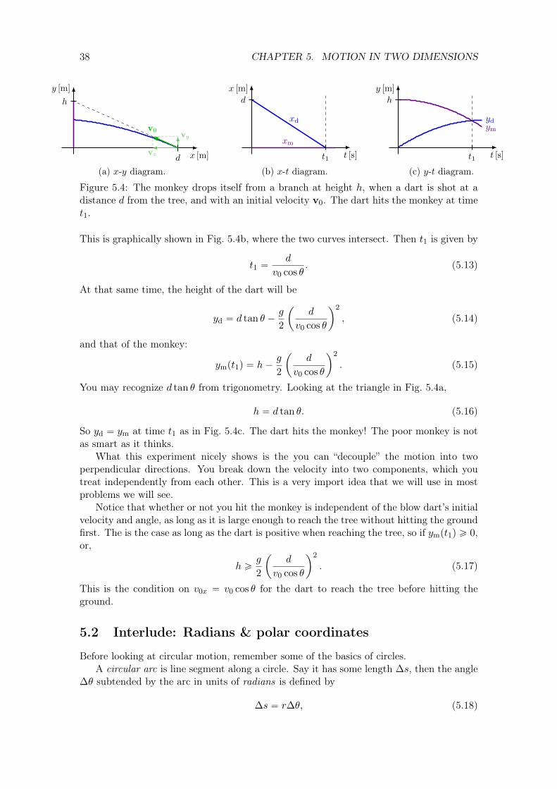
Figure 5.4: The monkey drops itself from a branch at height h, when a dart is shot at adistance d from the tree, and with an initial velocity v0. The dart hits the monkey at timet1.
This is graphically shown in Fig. 5.4b, where the two curves intersect. Then t1 is given by
t1 “d
v0 cos θ. (5.13)
At that same time, the height of the dart will be
yd “ d tan θ ´g
2
ˆ
d
v0 cos θ
˙2
, (5.14)
and that of the monkey:
ympt1q “ h´g
2
ˆ
d
v0 cos θ
˙2
. (5.15)
You may recognize d tan θ from trigonometry. Looking at the triangle in Fig. 5.4a,
h “ d tan θ. (5.16)
So yd “ ym at time t1 as in Fig. 5.4c. The dart hits the monkey! The poor monkey is notas smart as it thinks.
What this experiment nicely shows is the you can “decouple” the motion into twoperpendicular directions. You break down the velocity into two components, which youtreat independently from each other. This is a very import idea that we will use in mostproblems we will see.
Notice that whether or not you hit the monkey is independent of the blow dart’s initialvelocity and angle, as long as it is large enough to reach the tree without hitting the groundfirst. The is the case as long as the dart is positive when reaching the tree, so if ympt1q ě 0,or,
h ěg
2
ˆ
d
v0 cos θ
˙2
. (5.17)
This is the condition on v0x “ v0 cos θ for the dart to reach the tree before hitting theground.
5.2 Interlude: Radians & polar coordinates
Before looking at circular motion, remember some of the basics of circles.A circular arc is line segment along a circle. Say it has some length ∆s, then the angle
∆θ subtended by the arc in units of radians is defined by
∆s “ r∆θ, (5.18)

5.2. INTERLUDE: RADIANS & POLAR COORDINATES 39
r
r
∆θ
∆s
(a) x-t diagram.
x
y
(x, y) = (r; θ)
r
θ
x
y rθ
θ
rr
rr
(b) Polar coordinates and unit vectors.
x
y
11
11
−1−1
−1−1
0° 0
30°π6
(√32 ,
12
)
45°π4
(√22 ,
√22
)
60°
π 3
(12 ,
√32
)
90°
π2
120°2π3
(− 1
2 ,√32
)
135°
3π4
(−
√22 ,
√22
)
150°
5π6
(−
√32 ,
12
)
180°π
210°7π6
(−
√32 ,− 1
2
)22
5°
5π4(−
√22 ,−
√22
) 240°
4π 3
(− 1
2 ,−√32
)
270°
3π2
330° 11π6
(12 ,−
√32
)315° 7π4 (√
22 ,−
√22
)
300°5π3
(√32 ,− 1
2
)
(c) Summary of angle, sine and cosine values.
Figure 5.5: Some circle basics.
where r is the radius of the arc like in Fig. 5.5a. This allows for a more natural units forangles. The unit circle has radius r “ 1, such that its circumference is 2π, therefore in onefull rotation,
360˝ “ 2π rad « 6.283 rad. (5.19)
So1 rad “
180˝
π« 57.296˝, (5.20)
The definition of arc length is consistent: The total circumference of a circle is simply thelength of an arc spanning 360˝: ∆s “ 2πR.
A different way to describe a point P “ px, yq in a Cartesian coordinate system, is withpolar coordinates, here indicated with a semicolon:
P “ px, yq “ pr cos θ, r sin θq “ pr; θq. (5.21)
This is illustrated in Fig. 5.5b. The position vector in 2D points from the origin to P is
r “ xx` yy
“ r cos θx` r sin θy.
(5.22)(5.23)
However, we can also choose any two other unit vectors that are not parallel (i.e. linearlyindependent) to each other. For this chapter, it’s convenient to define the polar unitvectors, such that
r “ rrr` rθθ “ rr. (5.24)
Here the direction of the unit vectors depend on the angle θ: r points radially along theposition vector, while θ points perpendicular to r in the counterclockwise direction. Incase of the position vector r, only the radial component is nonzero rr “ r, while rθ “ 0.
Table 5.1: Angles in radians and degrees.
θ rrads θ r˝s sin θ cos θ tan θ
0 0 0 1 —1 180{π 0.841 0.540 1.557
π{6 30?
3{2 1{2?
3
π{4 45?
2{2?
2{2 1
π{3 60 1{2?
3{2?
3{3π{2 90 1 0 —π 180 0 ´1 0
3π{2 270 ´1 0 —2π 360 0 1 0

40 CHAPTER 5. MOTION IN TWO DIMENSIONS
Namely, θ is defined as the angle with the positive x axis in the counterclockwise direction.Written in terms of our trusty x and y:
r “ cos θx` sin θy
θ “ ´ sin θx` cos θy,
(5.25)
(5.26)
such that they both indeed have length 1:
|r| “ |θ| “a
cos2 θ ` sin2 θ “ 1, (5.27)
and are perpendicular to each other:
r ¨ θ “ 0. (5.28)
5.3 Uniform circular motion
Consider motion in a circle, like a satellite in orbit around the earth. Speed is the constantalong its orbit, but the direction of its velocity is changing so it is always tangential tothe orbit as in Fig. 5.6a. A change in velocity means there must be an acceleration. Theacceleration that keeps the satellite in a circular orbit is called the centripetal acceleration.It is orthogonal to the velocity vector, so it does not affect its length: The change is onlya “rotation” of the vector with respect to the center of the orbit.
If the velocity were constant in one direction, the satellite would move in a straight line.In that case, it would have travelled a distance d “ vt after some time t. From Fig. 5.6b,we see it has “fallen” a distance h instead, because of the centripetal acceleration. What ish? Notice from this figure that there is a right triangle, with sides about which Pythagorastells us that
pvtq2 ` r2 “ pr ` hq2 (5.29)
if the orbit is at a radius r. Rewriting,
pvtq2 “ 2rh` h2. (5.30)
For a very small time t, the fall height h is very small as well. We can therefore make theapproximation h2 ! hr, such that
pvtq2 “ 2rh. (5.31)
We can solve for h:
h «1
2
ˆ
v2
r
˙
t2. (5.32)
rθ
r
v
aω
(a) A constant centripetal acceleration is perpen-dicular to the velocity and changes it direction.
vtvv
v
hrr
rr
(b) A satellite orbiting the Earth due to gravitycreating a centripetal force.
Figure 5.6: Uniform circular motion.

5.3. UNIFORM CIRCULAR MOTION 41
Compare this to our familiar equation for a falling object
x “1
2at2, (5.33)
and we recognize that
a “v2
r(5.34)
This is known as the centripetal acceleration. This equation says that if the satellite wouldmove at twice the speed (2v), it would need four times the acceleration to stay in orbit atthe same radius r. On the other hand, for the same velocity v, but half the radius (r{2),it would need double the acceleration.
The direction of the acceleration points from the satellite’s position towards the center,so we can use the ´r unit vector, as in Fig. 5.5b:
Centripetal acceleration.
a “ ´v2
rr, (5.35)
The satellite completes one full circle in one period T . The distance travelled is 2πr,so it has a speed
v “ |v| “ 2πr
T. (5.36)
The period then can be expressed as
Period for uniform circular motion.
T “2πr
v. (5.37)
The number of times the satellite completes a full orbit per unit time is the frequencyf :
Frequency for uniform circular motion.
f “1
T“
v
2πr. (5.38)
Remember the period has units of seconds, so frequency has units 1{s.The angular velocity, or sometimes angular frequency, is the amount of radians, ∆s
covered per unit time. One full rotation is ∆s “ 2π, so
Angular velocity.
ω “ 2πf “2π
T“
dθ
dt(5.39)
Notice it can also be understood as the time derivative of the angle, analogous to positionx and velocity v. At a constant angular velocity,
ω “dθ
dt“θ ´ θ0
t´ t0. (5.40)
Assuming that θpt0q “ θ0 “ 0 at t0 “ 0, we see that

42 CHAPTER 5. MOTION IN TWO DIMENSIONS
Uniform rotation.θptq “ ωt. (5.41)
This indeed look familiar to uniform linear motion in Eq. (4.5): x “ vt.For uniform circular motion, the angular frequency is
Angular velocity for uniform circular motion.
ω “v
r. (5.42)
This allows us to express the velocity also as
v “ rω. (5.43)
The centripetal acceleration then, can be rewritten as
a “ ´rω2 (5.44)
We can derive Eq. (5.35) in a different way, starting from the position
Uniform circular motion.
rptq “ r cospωtqx` r sinpωtqy, (5.45)
where |r| “ r and ω are constant in time, and rp0q “ rx. The velocity they is given by
vptq “dr
dt“ ´rω sinpωtqx` rω cospωtqy. (5.46)
Similarly, the acceleration is
aptq “dv
dt“
d2r
dt2
“ ´rω cospωtqx`´rω sinpωtqy.
So we find,aptq “ ´ω2rptq “ ´ω2rrptq, (5.47)
such that the magnitude of the acceleration is
a “ ω2r (5.48)
Example 5.1: A satellite moves around the earth, close to the surface, just 100 km above.How long does it take to go around? The radius of the earth is
rC “ 6370 km. (5.49)
The radius of the satellite’s orbit therefore is r “ 6470 km. There is an acceleration due togravity, so the velocity to stay in orbit must be
v “?rg “ 7.97 km{s. (5.50)

5.4. MOTION ALONG A GENERAL PATH 43
vat
aca
θ
(a) The tangential acceleration at pointsalong v, while the tangential acceleration ac
is perpendicular.
r
r
ac
at
ac at
v
v
(b) A random path with curvature. The centripetal ac-celeration changes the direction of the velocity, while thetangential acceleration changes its speed.
Figure 5.7: The acceleration vector a can be broken into centripetal acceleration ac andtangential acceleration at.
Then the period is
T “2πr
v« 5100 s (5.51)
Which corresponds to about 85 min . The actual International Space Station is at anaverage height of about 400 km and takes 92 minutes to fully orbit the Earth.
5.4 Motion along a general path
The acceleration vector along a random path can be broken up into two components asshown in Fig. 5.7b: the tangential acceleration at, and the radial acceleration ar. Becausethe velocity vector is always tangential to the path, the tangential component appearswhen the speed v “ |v| along the path changes. The radial component on the other hand,is always perpendicular to the velocity (and the tangential acceleration), and causes thevelocity to change direction. This corresponds to the centripetal force in circular motion.One can always calculate the centripetal acceleration of a turn by measuring the radius ofcurvature, as shown in the dashed lines in Fig. 5.7b.

44 CHAPTER 5. MOTION IN TWO DIMENSIONS

Chapter 6
Laws of Motion & Forces
6.1 Momentum
The measure of motion an object has depends on its mass and velocity, and is known asits momentum, which is defined as:
Linear momentum (one dimension).
p “ mv “ mdx
dt(6.1)
If you have two object of different mass moving with the same velocity, the one with thelargest mass will have more momentum. The dimensions clearly are mass times lengthdivided by time, so one can use units kg m{s.
Just like velocity, it can be expressed as a vector with several components:
Linear momentum (vector).
p “ mv “ mdr
dt. (6.2)
6.2 Newton’s laws of motion
An unopposed force changes the direction of a mass, as prescribed by Newton’s laws ofmotion. Forces have a direction and magnitude, and are therefore represented by vectors.The unit of force is named after Isaac Newton (1643–1727):
N “kg m
s2 . (6.3)
The total force, also net or resultant force, on some object is the sum of all forces actingon it:
Ftot “ÿ
i
Fi. (6.4)
Now we are ready to look at Newton’s laws of motions that form the foundation ofclassical mechanics. Newton formulated these laws of motion in the Philosophiæ NaturalisPrincipia Mathematica around 1687. These laws allows us to understand motion of massesand better define what forces actually are.
45

46 CHAPTER 6. LAWS OF MOTION & FORCES
Newton’s laws of motion.
1. Law of inertia: An object either remains at rest, or continues to move in astraight line at a constant velocity, unless acted upon by a net force. If the netforce is zero, then :
dp
dt“ 0. (6.5)
2. A non-zero net force Fnet will change the momentum of an object, according to
Ftot “ÿ
i
Fi “dp
dt(6.6)
3. Law of action and reaction: When one object exerts a force F12 on a secondobject, the second object simultaneously exerts a force F21 equal in magnitudebut opposite in direction to the first object,
F12 “ ´F21 (6.7)
Notice that the way that we have written these laws, the first law is really just a specificcase of the second law, in which there is no net force and therefore a “ 0. A particle withno net force acting on it is a free particle. The first law implies that the momentum of afree particle is constant in time. This law encapsulates the concept of inertia, which is theresistance of any object with a mass to any change in its velocity. Some typical examplesare quickly pulling away a table cloth, without dragging everything on top of it with you.Or breaking off one sheet of toilet paper without having the whole roll unravel. It explainswhy objects in circular motion would fly off in a straight path, tangential to the circle,if the centripetal acceleration is suddenly removed. Finally, it is also the reason why youshould never attach a trailer to your car with a rope.
If all the forces on an object cancel, we get an equilibrium:
Mechanical equilibrium.Ftot “
ÿ
i
Fi “ 0. (6.8)
At equilibrium, the first law tells us that that the object will stay at rest, or its velocitywill be constant. A book that lies on a flat table is at equilibrium (see next section). Aladder leaning on a wall is at equilibrium. If you jump out of an airplane, very high up,the air resistance will grow with your speed until it balances the force of gravity, and youreach a terminal velocity, which is constant. At this point, the force of gravity and theforce of wind resistance would cancel out, and you would be moving as a free particle withconstant velocity.
We know that p “ mv, such that in general
Ftot “dp
dt“ m
dv
dt`
dm
dtv. (6.9)
In most cases, m is constant, so the second term, which is the time derivative of the mass,vanishes, and we find the most well-known form of F “ ma:

6.3. GRAVITATIONAL FORCE 47
Newton’s second law for constant mass.
Ftot “ mdv
dt“ m
d2r
dt2“ ma. (6.10)
The third law is all about action and reaction. When you push on a wall, the wallpushes back. If your force acting on the wall is F12, then the wall pushes on you witha force F21 “ ´F12. Similarly, when you ride a skateboard, and you push the groundbackwards with your foot, the ground pushes you forward in return. Another example isrecoil : When you shoot a bullet, the gun will push you back as it repels the bullet and hotgas and metal go forward.
6.2.1 Interlude: Algorithm to solving forces
Students who just learn about forces and Newton’s laws often do not know where tostart on a physics problem with forces. Typically you can use the following algorithm tosystematically solve them:
1. Make a drawing and understand what is going on: What are the moving parts (degreesof freedom like positions and angles)? What are the forces on what object? Is therean equilibrium or balance between forces? Use Newton’s first law.
2. Write down for each mass the total forceř
Fi and apply Newton’s second law.Choose a coordinate system or positive direction to simplify breaking down the forcevector into components.
3. Note what is given and known, and what is unknown. Typically you need at leastn independent equations to solve for n unknowns. Often you can use geometricequations to solve for angles or lengths.
4. Finally, sanity check and interpretation: Does the answer make sense? How does itdepend on other variables? What is the physical interpretation of the result?
Similar steps can be used for a lot of other basic physics problems. Now let’s look at someexamples.
6.3 Gravitational force
The most common force in our lives is called weight, and results from the force of grav-ity,
Weight.weight “ Fg “ mg. (6.11)
Here on Earth, the gravitational acceleration is around g « 9.8 m{s2. We can write it as avector:
Fg “ mg. (6.12)
Where F and g both point downward to the center of the earth.In general, however, two points of massm andM attract each other according to

48 CHAPTER 6. LAWS OF MOTION & FORCES
Newton’s law of universal gravitation.
Fg “ ´GmM
r2r, (6.13)
where r is the distance between the mass points. So the attractive force depends on theinverse of the distance squared: Gravity is four times weaker at double the distance, etc.The minus sign indicates attraction.
By comparing Eq. (6.11) to (6.11) to, we see that actually
g “MG
r2. (6.14)
So the size of g actually depends on the distance to the center of the Earth, and the Earth’smass. Actually, it also depends on the shape and mass density around you. Typically weassume that the Earth is spherically symmetric, which is good enough as a first-orderapproximation. It even allows us to approximate the Earth as a simple mass point with noradius. In reality, the Earth is slightly “flattened” and bulges a bit at around the equatordue to its rotation. Furthermore, land masses tend to be more dense and stick further outof the “ideal surface”. We will learn later more about mass distributions of general bodiesand centers of gravity.
Gravity is a nice example of a force field. A field in physics is a value (with units)as a function of space. A field can be a scalar field or a vector field. A scalar fieldfpx, y, zq “ fprq takes on a single scalar value everywhere in space, with no direction,and we will see some examples in later chapters on potential energy. The earth creates agravitational field
g “ ´gz, (6.15)
,if z points down, which is a vector field which acts on masses. In this case, close to Earth’ssurface, it is a simple uniform field : Its magnitude stays almost constant and points in onedirection only, downward. At a larger scale, the earth creates a gravitational field
gprq “ ´MG
r2r, (6.16)
which only depends on the distance from Earth’s center.
6.4 Normal force
When an object with mass m rests on a table, something must counter the gravitationalforce to hold it in place. This is the normal force FN (or just N in some textbooks) thetable’s surface exerts on the mass. Because the objects stays put, all forces on the objectmust cancel:
ÿ
i
Fi “ FN ` Fg “ 0. (6.17)
myFN
Fg = −mgy
(a) The forces on a mass m at rest: The surface exerts anormal force FN, and the Earth a gravitational one, Fg.
FN Fg = −mgy
(b) The normal and gravitational forcevectors create a balance.
Figure 6.1: Normal force.

6.4. NORMAL FORCE 49
my
F
FN
Fg = −mgy
(a) A person pulls up amass with force F.
FN
FFg = −mgy
(b) At equilibrium,the forces cancel.
FFg = −mgy
ma
(c) Forces not cancelingcause an acceleration.
Applied force F
Normal
forceFN
FN =
F ≤mg
FN = 0 ≤ mg ≤ F
mg
mgstatic kinetic
(d) The normal force becomes smaller asthe applied F becomes larger.
Figure 6.2: Normal force.
It is called “normal” because it is orthogonal to the surface. In the simplest case of Fig. 6.1a,this is a one-dimensional problem, so fixing the y axis along the vertical, we have
FN “ FNy
Fg “ ´mgy.
(6.18)(6.19)
SoFNy ´mgy “ 0, (6.20)
or simply,FN ´mg “ 0. (6.21)
So the normal force is simply the weight!
FN “ mg. (6.22)
For example, if your mass is 80 kg, the normal force is about 784 N. On the moon, wheregK “ 1.625 m{w2 “ 0.167g, you would weigh 130 N, i.e. any scale calibrated to Earth’sgravity would read 13 kg.
Remember that due to the third law, the book also pushes on the table, so the tableexperiences a force ´mgy from the book.
Now, let’s make it a bit more complicated. Imagine you slowly start pulling up themass with a force F , as in Fig. 6.2a. You build up the force, and before applying enoughto lift it up from the ground, you still maintain an equilibrium:
ÿ
i
Fi “ FN ` Fg ` F “ 0, (6.23)
orFN ´mg ` F “ 0, (6.24)
where we assumed F is in the positive vertical directions. This time, the normal force isless than the weight mg:
FN “ mg ´ F. (6.25)
When you reach enough force to lift the mass from the ground, the normal force disappears.This is shown in Fig. 6.2d. At this points, the forces do not balance anymore, and you getan acceleration upward, given by
ÿ
i
Fi “ Fg ` F “ ma. (6.26)

50 CHAPTER 6. LAWS OF MOTION & FORCES
x0
`0
m
(a) Rest length `0.
x0
`0x
m
F
(b) Extension.
x0
`0−x
m F
(c) Compression.
Figure 6.3: Spring with a mass.
`0
(a) Without a mass, the spring has length `0.
m
F
mg
`0
∆`
(b) Elongation ∆` due to gravity.
Figure 6.4: Hanging spring with rest length `0.
6.5 Springs & Hooke’s law
A spring pulls when extended, and pushes when compressed. It always “wants” to returnto its rest length `0. It does so with a force F , that is proportional to the change in lengthx shown in Fig. 6.3:
Hooke’s law.F “ ´kx. (6.27)
The constant of proportionality k is the spring constant, which depends on the spring inquestion. This constant is a measure of the “stiffness” of the spring. The larger k, thestronger the spring will try to return to its rest length. The minus sign indicates that thespring’s force points towards x “ 0. Not all springs follow Hooke’s law; those that do arecalled Hookian.
Consider a mass hanging on a string as in Fig. 6.4. The weight from the mass willcause the spring to be extended a little bit to some length `0 ` ∆`. At equilibrium, thespring force and weight balance
ÿ
i
Fi “ F`mg “ 0, (6.28)
or,0 “ k∆`´mg, (6.29)
such that the extension is given by∆` “
mg
k. (6.30)
6.6 Tension
Now consider a mass m hanging on a string or rope suspended from the ceiling, like inFig. 6.5a. The string pulls the mass with a force called the tension. Tension is very similar
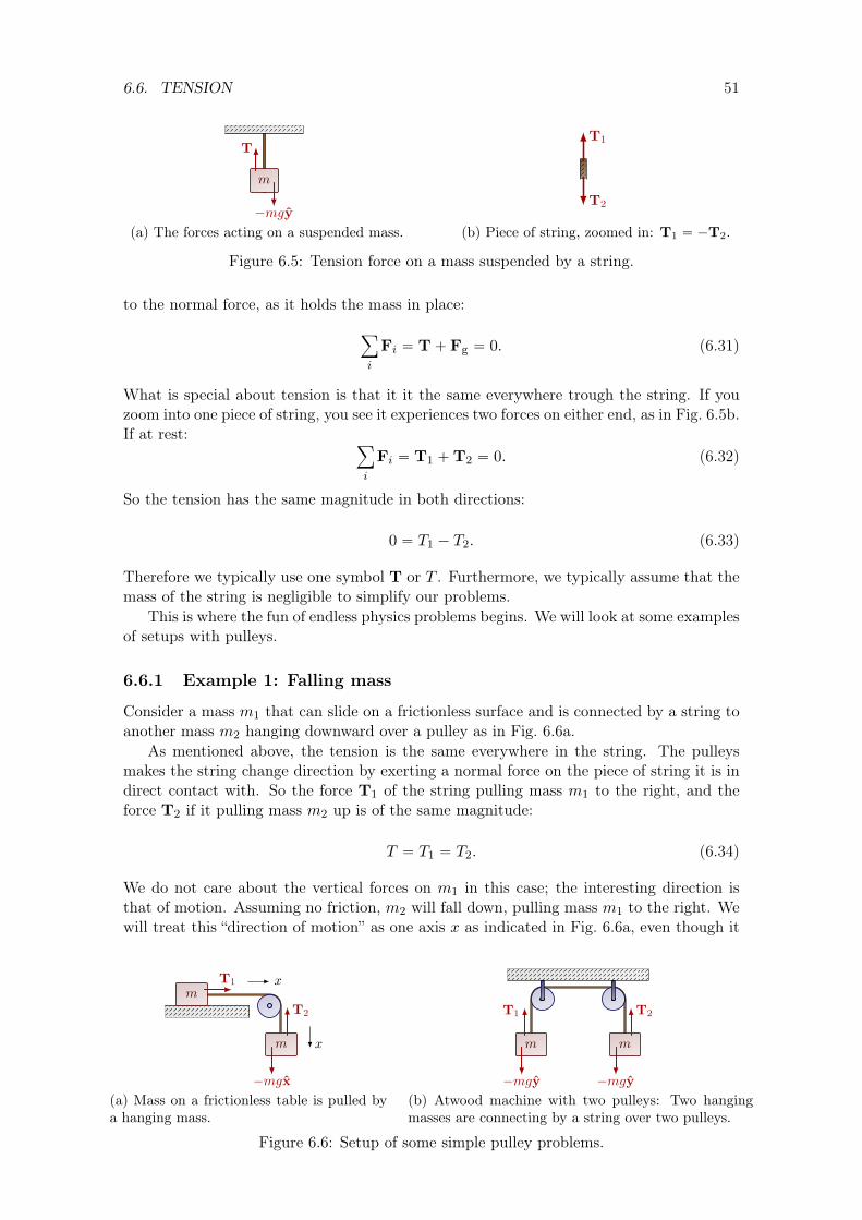
6.6. TENSION 51
m
T
−mgy
(a) The forces acting on a suspended mass.
T1
T2
(b) Piece of string, zoomed in: T1 “ ´T2.
Figure 6.5: Tension force on a mass suspended by a string.
to the normal force, as it holds the mass in place:
ÿ
i
Fi “ T` Fg “ 0. (6.31)
What is special about tension is that it it the same everywhere trough the string. If youzoom into one piece of string, you see it experiences two forces on either end, as in Fig. 6.5b.If at rest:
ÿ
i
Fi “ T1 `T2 “ 0. (6.32)
So the tension has the same magnitude in both directions:
0 “ T1 ´ T2. (6.33)
Therefore we typically use one symbol T or T . Furthermore, we typically assume that themass of the string is negligible to simplify our problems.
This is where the fun of endless physics problems begins. We will look at some examplesof setups with pulleys.
6.6.1 Example 1: Falling mass
Consider a mass m1 that can slide on a frictionless surface and is connected by a string toanother mass m2 hanging downward over a pulley as in Fig. 6.6a.
As mentioned above, the tension is the same everywhere in the string. The pulleysmakes the string change direction by exerting a normal force on the piece of string it is indirect contact with. So the force T1 of the string pulling mass m1 to the right, and theforce T2 if it pulling mass m2 up is of the same magnitude:
T “ T1 “ T2. (6.34)
We do not care about the vertical forces on m1 in this case; the interesting direction isthat of motion. Assuming no friction, m2 will fall down, pulling mass m1 to the right. Wewill treat this “direction of motion” as one axis x as indicated in Fig. 6.6a, even though it
m
m
x
x
T1
T2
−mgx(a) Mass on a frictionless table is pulled bya hanging mass.
m m
T1 T2
−mgy −mgy(b) Atwood machine with two pulleys: Two hangingmasses are connecting by a string over two pulleys.
Figure 6.6: Setup of some simple pulley problems.

52 CHAPTER 6. LAWS OF MOTION & FORCES
changes “true direction” due to the pulley. We can write down Newton’s second law foreach mass in this direction of motion:
#
m1a1 “ T1 (mass 1)m2a2 “ m2g ´ T2 (mass 2)
(6.35)
Because the two masses are connected by the string they will have the same acceleration:If the m1 moves by a distance ∆x, m2 moves by a distance ∆x, if the m1 moves at a speedv, m2 moves at a speed v, and the same goes for the acceleration. This works as long aswe assume the string is not stretchy. So a “ a1 “ a2. We then find that
$
&
%
m1a “ T
a “m2
m1 `m2g
(6.36)
So in case m1 “ m2, a “ g{2.
6.6.2 Example 2: Two masses balancing over pulleys
Now consider an Atwood machine with two pulley as in Fig. 6.6b: Two masses hang by astring that connects them over two pulleys. This time, we write:
#
m1a “ T ´m1g (mass 1)m2a “ m2g ´ T (mass 2)
(6.37)
Here we again have chosen the positive direction by setting an axis that follows the ropefrom m1 to m2. (Alternatively, we could have chosen the vertical y axis and set a1 “ ´a2,which means that if one mass accelerates in direction, the other accelerates in the opposite.)Given m1, m2 and g, we have two unknowns: T and a. But we have two equations, so wecan solve it easily:
$
’
’
&
’
’
%
a “T
m1´ g “ g
T “2m1m2
m1 `m2g
(6.38)
In case m “ m1 “ m2, T “ mg and a “ 0, which makes sense.
m1m3
m2
θ1 θ3T1
T2
T3
−m1gy −m2gy
−m3gy
(a) Setup of the masses, strings and pulleys,and the forces acting on each mass.
T1
T3
T2
θ1 θ3
(b) Forces on the point wherethe three strings meet.
(4 kg)g
T1
(3 kg)g T3
(5 kg)g
T2
(c) The tensions form a righttriangle for 5 : 4 : 3 ratios.
Figure 6.7: Third example of masses with strings and pulleys.

6.7. CENTRIPETAL FORCE 53
6.6.3 Example 3: Three unequal masses
Finally, look at Fig. 6.7a: Three masses are connected by strings, suspended by pulleys.We assume this system is in equilibrium. There are three tensions,
T1 “ m1g
T2 “ m2g
T3 “ m3g.
(6.39)(6.40)(6.41)
The interesting point is where the three strings meet, as in Fig. 6.7b:
T1 “ ´T1 cos θ1x` T1 sin θ1y
T2 “ T2 cos θ3x` T2 sin θ3y
T3 “ ´T3y.
(6.42)(6.43)(6.44)
What are these angles θ1 and θ3? We can write down Newton’s law to obtain two equationthat can be solved for these two unknown angle if the masses are given:
#
0 “ ´T1 cos θ1 ` T2 cos θ3
0 “ T1 sin θ1 ` T2 sin θ3 ´ T3
(6.45)
As we saw in class, a special combination is when m1 “ 4 kg, m2 “ 5 kg and m2 “ 3 kg,in which case the two top strings will form a right angle, because the tension vectors willform a right triangle with sides of 5 : 4 : 3 ratios.
6.7 Centripetal force
If you hold a bucket with water upside down, the water will pour out. But if you spin itaround vertically and fast enough, the water will stay in the bucket. This is a consequenceof the first law: The water has some velocity and because of its inertia, it wants to movein a straight line. However, there is a non-zero net force that “pushes” the water to changedirection to stay in a circle path. This is the bottom of the bucket pushing the water. Thisis called the centripetal force Fc, which provides the centripetal acceleration we have seenin Section 5.3.
Other examples include the Earth orbiting the sun, where gravity acts as the centripetalforce, or a mass m on a string you sling around very fast around your head. If it is theonly force, the mass will move with a constant speed v in a circle with constant radius r.This is illustrated in Fig. 6.8.
You may have heard about the centrifugal force. This is the force the water “feels” whenit is being swung around, and you might also experience it when a car takes a sharp turn,or you ride a roller coaster. This is however not a real force, but rather a pseudoforce. It isthe consequence of being accelerated, while your inertial mass wants to move in a straightline. In the frame of reference of the water or car passenger, it seems like there is a forcepulling it. We will talk more about inertial frame of references in Section 8.4.
r
mFc
a
v
Figure 6.8: A constant centripetal force keeps a mass moving in a circle with constantradius r and tangential velocity v.

54 CHAPTER 6. LAWS OF MOTION & FORCES
h
r m
L
θx
y
T
−mgy
ma
(a) A massm on a string of length L swings in cir-cles of radius r. There are two forces: the tensionand weight.
m
Ty
Tx
T
−mgyma
θ T−mgy
ma
θ
(b) Breakdown of the forces on the mass: They donot balance and the tension causes a centripetalacceleration a.
Figure 6.9: Example of a mass on a string.
6.7.1 Example: Mass on a string
Suppose you have a mass m hung on a string being slowly swung around in circles of radiusr like in Fig. 6.9a. What is the angle of the string with the horizontal as a function ofthe string’s length L and the angular frequency ω? There are two forces, the tension andgravitational force:
ÿ
F “ T`mg “ ma. (6.46)
We know the velocity changes direction, because the centripetal force “pulls” the mass intoa circular motion. So a is not zero. Choosing the coordinate system as in Fig. 6.9a, theforces can be decomposed into
$
&
%
mv2
r“ T sin θ
0 “ T cos θ ´mg
(6.47)
Here we have used the fact that that the tension in the string will balance the gravitationalforce in the y direction to hold it at the same height (or equivalently, at the same angle θ),and simultaneously provide a centripetal force in the x direction:
a “ axx` ayy
“v
mx.
(6.48)
(6.49)
By comparing the two formula in Eq. (6.47), we find that
v2
r sin θ“
g
cos θ. (6.50)
Therefore,
tan θ “v2
rg“rω2
g, (6.51)
where we have used v “ rω. We can find yet another independent equation by looking atthe right-angled triangle made by the string with the horizontal:
tan θ “r
h. (6.52)
Comparing Eqs. (6.51) and (6.52), we get
ω2 “g
h. (6.53)

6.8. FRICTION 55
To find θ, we can substituting in h “ L cos θ,
ω2 “g
L cos θ, (6.54)
orθ “ acos
´ g
ω2L
¯
. (6.55)
The acos function is a monotone decreasing function, so this equation says the faster themass swings around (larger ω, smaller 1{ω2), the larger the angle θ, which makes intuitivesense.
6.8 Friction
Up until now we have assumed that our surfaces were frictionless. In reality, most surfacesare not infinitely smooth, so there will be a frictional force Ff (sometimes just f), pointingin the opposite direction of motion. Imagine you push or pull a mass across the groundwith a force F , then friction will counteract the force of your push or pull. It turns outthat friction is proportional to the normal force: If the block’s mass is twice as large, thefrictional force is twice as large as well. There will be a constant of proportionality µ thatdepends on the materials involved:
Friction during motion.Ff “ µFN. (6.56)
The direction will always be parallel to the surface an in the opposite direction of motion.The constant µ is the unitless coefficient of friction, and takes values between 0 and 1.µ “ 0 corresponds to no friction, and µ “ 1 to maximal friction. Each combination oftwo materials has two coefficients: the static coefficient of friction µs, and the kineticcoefficient of friction µk. Table 6.1 lists some concrete values of familiar materials. Thestatic coefficient is only important if the object is pushed from rest to motion. Once in
m
y
xFN
−mgy
FFf
(a) Pushing a mass.
m
y
x
FN
−mgy
F
Ff
(b) Pulling a mass.
F f=F≤ µ
sFN Ff = µkFN ≤ F
Applied force F
FrictionforceFf
µsFN
static kinetic
(c) Two regimes of friction Ff , depending onthe applied force F .
Figure 6.10: Frictional force Ff counteracts the applied force F. Once F ą µsFN, thefriction cannot balance the applied force, and the mass starts moving with a constantfriction Ff “ µkFN.
Table 6.1: Static and kinetic coefficient of friction for several combinations of materials.
Materials µs µk
Wood on wood 0.25–0.5 0.2Steel on steel 0.74 0.57Teflon on steel 0.04 0.04
Ice on ice 0.1 0.03Synovial joint 0.01 0.003

56 CHAPTER 6. LAWS OF MOTION & FORCES
m
θ
x
y FN
Ff
mg sin θ
−mg cos θmg
θ
(a) There are three forces on the mass: the normalforce, friction and weight.
−mg cos θ
mg sin θ
mg
FN
Ff
θ
(b) The forces on the mass balance, as long asfriction cancels the x component of the weight.
Figure 6.11: Frictional force on a mass on an inclined plane.
motion, the kinetic coefficient comes into play. Typically µs ą µk: Once there is motion,the friction becomes a reduced a little bit. In case the force F ă µsFN, the block stays atrest, and
Friction at rest.Ff “ F ă µsFN. (6.57)
This is plotted in Fig. 6.10c.
6.8.1 Example: Friction on an inclined plane
Now, let’s look at an example where the table if inclined with some angle θ with respectto the horizontal. If the angle is small, friction will hold the block of mass in place, but ifthe angle is large enough, the block will start to slide down, due to gravity. What is thecritical angle θc at which this happens? First we identify the three forces acting on themass:
ÿ
Fi “ Fg ` Ff ` FN. (6.58)
This is clearly a two dimensional problem, so we break down the vectors into their com-ponents. It is convenient to use a coordinate system with the x axis pointing downwardalong the table’s plane, and the y axis perpendicular to it, like in Fig. 6.11a. The y axisnow makes an angle θ with the vertical, so gravity will have a x and y component:
Fg “ Fgxx` Fgyy
“ mg sin θx´mg cos θy.
(6.59)(6.60)
Notice that if θ “ 0, the x component disappears, just as expected. Assume θ is smallenough for the block to stay at rest. Then
#
0 “ Fg ´mg cos θ
0 “ FN `mg sin θ ´ Ff
(6.61)
are the conditions for equilibrium. Because the normal force FN is pointing upward andperpendicular to the table, and the friction Fg point opposes the x component of gravitythat would make the object slide. To stay at rest, we have the condition
mg cos θ “ Fg ă µsFN. (6.62)

6.8. FRICTION 57
This defines the critical point at which the block starts sliding:
mg cos θc “ Fg “ µsFN. (6.63)
Substituting this into Eq. (6.61), we find
µ “ tan θc. (6.64)
This result allows us to measure µs for any combination of materials by measuring thecritical angle θc when the block starts sliding. The larger µs, the larger the critical angleθc at which the mass starts to move.
6.8.2 Drag
Drag is the frictional force due to air resistance.Consider an airplane flying at a constant velocity. Simplified, it experiences four forces:
• Gravity Fg pulling the plane downward, as usual.
• Thrust Fthrust by the engines propelling the airplane forward.
• Drag Fdrag opposing the thrust due to air resistance.
• Lift Flift by the wings, pushing the airplane upward.
What is special about the drag force is that it depends on the velocity. In simple cases, itis proportional to the cross-sectional area of the plane and the velocity squared:
Fdrag9Av2. (6.65)
Take for example two planes with the same engine (so the same thrust), but one with anarea two times as large, A1 “ 2A2. Flying at constant speeds, what will their velocities berelative to each other? Since the thrust are the same, the drag forces have to be the same.We can therefore find that
Fdrag,1 “ Fdrag,2
CA1v21 “ CA2v
22
A1v21 “
1
2A1v
22
where C is some constant that is the same between both planes. So v2 “?
2v1. If the“wider” plane is moving with a speed v1 „ 800 kmh, the smaller plane with the same thrustwill fly at v2 „ 1130 kmh.

58 CHAPTER 6. LAWS OF MOTION & FORCES

Chapter 7
Work & Energy
7.1 Work
In this chapter, we are going to discuss the relationship between force and energy. Recallthe units of force are
N “kg.m
s2, (7.1)
which is easy to remember using F “ ma. Now, the units of energy are Joules:
J “kg.m2
s2“ N m (7.2)
In fact, the amount of energy that is transferred to an object by a force F by moving itover a distance ∆x can be defined as
W “ F∆x. (7.3)
This is the work performed by the force F , see Fig. 7.1a. And indeed, work allows usto define the amount of energy that objects can possess. Next semester we will also seeanother type of energy transfer, namely by heat in thermodynamics.
Equation (7.3) is a simple case where the displacement is parallel to the force. Workcan be positive or negative: It is positive if the force,F , points in the same direction as thedisplacement, and negative if they are opposite. More generally, the force vector F anddisplacement vector ∆x may not be parallel, as in Fig. 7.1b:
Work. The work done by a force F to move another object by a displacement ∆xis
W “ F ¨∆x “ F∆x cos θ, (7.4)
where θ is the angle between F and ∆x.
Notice that F cos θ can be interpreted as the component of F that is along the ∆x direction,which is why the scalar product is so useful here. We see that if 0 ă θ ă π{2, the workwill be positive because cos θ ą 0 (Fig. 7.1b), while if π{2 ă θ ă 3π{2, the work willbe negative (cos θ ă 0, see Fig. 7.1c). If the force and displacement are perpendicular toeach other, W “ F ¨∆x “ 0, the work will be zero: The force F cannot not cause anydisplacement in the ∆x direction.
59
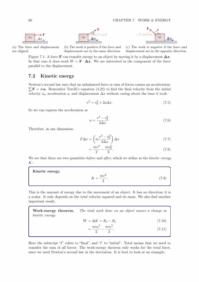
60 CHAPTER 7. WORK & ENERGY
m ∆xF
(a) The force and displacementare aligned.
m ∆xF cos θ
Fθ
(b) The work is positive if the force anddisplacement are in the same direction.
m ∆x−F cos θ
F θ
(c) The work is negative if the force anddisplacement are in the opposite direction.
Figure 7.1: A force F can transfer energy to an object by moving it by a displacement ∆x.In that case it does work W “ F ¨∆x. We are interested in the component of the forceparallel to the displacement.
7.2 Kinetic energy
Newton’s second law says that an unbalanced force or sum of forces causes an acceleration:ř
F “ ma. Remember Torelli’s equation (4.22) to find the final velocity from the initialvelocity v0, acceleration a, and displacement ∆x without caring about the time it took:
v2 “ v20 ` 2a∆x. (7.5)
So we can express the acceleration as
a “v2 ´ v2
0
2∆x. (7.6)
Therefore, in one dimension:
F∆x “
ˆ
mv2 ´ v2
0
2∆x
˙
∆x
“mv2
2´mv2
0
2.
(7.7)
(7.8)
We see that there are two quantities before and after, which we define as the kinetic energyK:
Kinetic energy.
K “mv2
2. (7.9)
This is the amount of energy due to the movement of an object. It has no direction; it isa scalar. It only depends on the total velocity squared and its mass. We also find anotherimportant result,
Work-energy theorem. The total work done on an object causes a change inkinetic energy:
W “ ∆K “ Kf ´Ki
“mvf
2
2´mvi
2
2.
(7.10)
(7.11)
Here the subscript “f” refers to “final”, and “i” to “initial”. Total means that we need toconsider the sum of all forces: The work-energy theorem only works for the total force,since we used Newton’s second law in the derivation. It is best to look at an example.

7.2. KINETIC ENERGY 61
m
F
mg ∆y
Figure 7.2: Arnold lifts up a weight of mass m to a height h with a constant force F . Thedisplacement vector is ∆y “ hy.
7.2.1 Example: Lifting a weight
Consider Arnold lifting a block mass m “ 5 kg by a height h “ 2 m with a force F “ 500 N.There are two forces: the one by Arnold, and the weight due to gravity, see Fig. 7.2. Severalquestions come up:
1. What is the work done by Arnold?
2. What is the work done by gravity?
3. What is the final velocity of the block?
The answers are simple enough:
1. Arnold’s force is parallel to the displacement, θ “ 0, so WA “ Fh cos θ “ 1000 J.
2. Gravity opposes the displacement, θ “ 180˝, so Wg “ mgh cos θ “ ´100 J.
3. The total work on the block is Wtot “ 900 N “ ∆K, so the final velocity upwards is
vf “
c
2Wtot
m“ 19
m
s. (7.12)
If Arnold moved the block with a constant force F , then this would be the final velocityvf at height h.
7.2.2 Work integral over a path
So far we have only looked at a constant force F . In this case the work, W “ F∆x, canbe thought of as the blue area in Fig. 7.3a. If the force F “ F pxq varies as a function ofdisplacement x, we can use an integral
W “
ż x2
x1
Fdx. (7.13)
W
xx1 x2
F∆x
(a) A constant force F .
W
xx1 x2
F
dx
(b) A general force F .
Figure 7.3: Work is the integral of F ¨ x over dx.

62 CHAPTER 7. WORK & ENERGY
ds
dsF F
θ
θ
A
B
(a) A general path.
a
bA
B
(b) A closed path.
Figure 7.4: Integral.
Even more generally, the moved object can follow a three-dimensional path where thedirection of the displacement and force varies as illustrated in Fig. 7.4a. Let’s call s thedistance along the path, and the vector ds a small displacement that is tangential to thepath.1 In three dimensions,
ds “ dxx` dyy ` dzz. (7.14)
The work done by the vector Fpsq is the integral along the path
Work along a path.
W “
ż s2
s1
F ¨ ds , (7.15)
with ds as the differential element. This is a line integral. Notice that we are actually onlyinterested in the component of the force F that is parallel to the displacement ds,
F ¨ ds “ Ft ds , (7.16)
where Ft is the component of F that is tangential to the path. And of course, ds is alsoparallel to the path, with ds being the length of ds.
Let’s demonstrate the work-energy theorem for this general path. We want to arriveat Eq. (7.11), so we need to retrieve the velocity from somewhere. We can use Newton’ssecond law:
Fpsq “ ma “ mdv
dt, (7.17)
where v is the velocity along the path, such that
v “ds
dt. (7.18)
Remember from Section 5.4 that only the tangential acceleration changes the magnitude ofthe velocity vector. The tangential acceleration at is caused by the tangential componentFt, so:
Ftpsq “ mat “ mdv
dt. (7.19)
We can now solve the integral (7.15) by substituting ds with dv using the chain rule
dv
dt“
dv
ds
ds
dt“
dv
dsv. (7.20)
SoFtpsq ds “ mv dv . (7.21)
1Not to be confused with the rptq, the radial distance to the origin, and rptq, the accompanying positionvector, which points from the origin to a point along the path.

7.3. CONSERVATIVE & NON-CONSERVATIVE FORCES 63
and we solve the integral
W “
ż vf
vi
mv dv
“mvf
2
2´mvi
2
2,
(7.22)
(7.23)
where we integrate over v and set the limits to vi “ vps1q and vf “ vps2q. We have shownthat the work-energy theorem also holds for our path integral:
Work-energy theorem for a general path.
W “
ż s2
s1
F ¨ ds “mvf
2
2´mvi
2
2. (7.24)
Again, because we used Newton’s second law in the derivation, W has to be the total workdone by the total force.
Sometimes it might be useful to write this integral in a time dependent way. UsingEq. (7.18),
Work time-integral.
W “
ż t2
t1
F ¨ v dt. (7.25)
This can be used if F ptq and vptq are known as a function of time.
7.3 Conservative & non-conservative forces
Suppose we want to move a mass from point A to B. There might be several paths we cantake, as illustrated in Fig. 7.4b. Ask yourself: Is the total work different on different paths?The answer depends on the type of force: A force is called conservative if the work is thesame for any path between two points. Otherwise, if the work is different for differentpaths, the force is called non-conservative.
So for a conservative force, the work Wa and Wb along paths a and b in Fig. 7.4b,respectively, is the same:
Wa “Wb. (7.26)
This implies we can move back in a loop, such that the total work is zero!
Wtot “Wa ´Wb “ 0 (7.27)
For any path:
Work of conservative force on a closed path.
W “
¿
F ¨ ds “ 0. (7.28)
The circle on the integral symbol indicates the path is closed. Let’s make it a bit moreconcrete by looking at some examples.

64 CHAPTER 7. WORK & ENERGY
a
b
c
d
y
xx1 x2
y1
y2
F = −mgy
(a) A closed path in a gravitationalforce field.
y
x1 2 3 4
1
2
3
4
(0, 0) = A
B = (2, 4)
F = yx+ x2ya
b
(b) A closed path in a non-conservativefield.
Figure 7.5: Paths in force fields.
7.3.1 Example 1: Gravity
As discussed in Section 6.3, gravity provides a uniform vector field for a mass m:
Fg “ ´mgy. (7.29)
It is constant in size and direction everywhere. Suppose you follow a closed path as inFig. 7.5a. It has four segments: moving left (a), up (b), right (c) and down (d). It is easyto compute the work performed by gravity in this rectangular loop. We can break up theloop integral into its four segments:
W “
¿
F ¨ ds
“
ż x2
x1
F ¨ x dx`
ż y2
y1
F ¨ y dy `
ż x1
x2
F ¨ x dx`
ż y1
y2
F ¨ y dy .
(7.30)
(7.31)
The horizontal segments, a and c, are perpendicular to gravity, so do not contribute. Onlythe vertical ones remain, but cancel each other:
W “ ´mgpy2 ´ y2q ´mgpy1 ´ y2q “ 0. (7.32)
So the total work done on a mass making a loop is zero. Therefore, gravity is a conservativeforce.
7.3.2 Example 2: F “ yx ` x2x
Now consider the vector fieldF “ yx` x2y. (7.33)
Is this force conservative? Let’s look at an arbitrary loop in the xy plane. Consider patha following y “ 2x, and path b following y “ x2. They both start at A “ p0, 0q and meetin B “ p4, 2q. To compute the work, one can integrate over each component separately,using the fact that ds “ dxx ` dyy, so we get two terms for the work in the x directionand in the y direction:
W “
ż 2
0y dx`
ż 4
0x2 dy
First compute the work along path a by rewriting the integral using the constraint y “ 2xor x “ y{2:
Wa “
ż 2
02x dx`
ż 4
0
´y
2
¯2dy “
28
3.

7.4. POTENTIAL ENERGY 65
Compare to the work along path b with relation y “ x2:
Wb “
ż 2
0x2 dx`
ż 4
0y dy “
32
3.
They are not the same! The work done depends on the path that was taken. We haveproven by counterexample that this force is not conservative.
7.4 Potential energy
When defining work, we mentioned that energy is transferred to the moved object. Infact, for conservative forces, you can “store” energy in an object, which can be reused later.Notice that potential energy is negative of the work done by the force. This type of energyis called potential energy.
Potential energy.∆U “ Uf ´ Ui
“ ´W “ ´
ż s2
s1
F ¨ ds
(7.34)
(7.35)
7.4.1 Gravitational potential energy
Gravity is the classic example. When Arnold lifts up the mass in Fig. 7.2, gravity as aconservative fore will do negative work, so it will add positive gravitational potential energyto the mass. Arnold lifted the mass from a lower to a higher potential. The difference,from the formula for potential energy, is
∆U “ ´
ż h
0p´mgqdy “ mgh. (7.36)
The minus sign in the integrand indicates that the gravity opposes the vertical displace-ment. Like the example in Section 7.3.1, only the height difference h is important.
Gravitational potential energy difference.
∆U “ mgy2 ´mgy1 “ mgh, (7.37)
where h “ y2 ´ y1. This is also clear by performing an indefinite integral;
Upyq “
ż
mgdy “ mgy ` U0, (7.38)
where U0 is an integration constant. In a nice box:
Gravitational potential energy.
Upyq “ mgy ` U0, (7.39)

66 CHAPTER 7. WORK & ENERGY
This constant U0 is somewhat arbitrary and can be set to anything you like. In the problemwith Arnold, it is natural to choose the ground for setting
U0 “ Up0q “ 0. (7.40)
Here, y “ 0 is our chosen reference level where we set Up0q “ 0. It is clear that Upyq ą 0is positive as long as y ą 0, and negative if y ă 0.
We can calculate the potential energy more generally for a gravitational force. Remem-ber the force between two masses is
Fgprq “ ´GmM
r2r. (7.41)
The only interesting direction is radial, and clearly
r ¨ ds “ dr. (7.42)
The work a mass does to attract another mass from distance r1 to r2 by means of gravityis positive if r2 ă r1 because the force and displacement are aligned:
W “
ż r2
r1
GmM
r2dr “ G
mM
r1´G
mM
r2. (7.43)
Note this result also holds for r2 ą r1, when the work becomes negative. It is veryconvenient to set a reference point r1 at infinity, such that the first term disappears:
limrÑ8
GmM
r“ 0. (7.44)
So for this common choice,
Gravitational potential energy.
Uprq “ ´GmM
r. (7.45)
Notice that this form of the potential energy is always negative, because it is always lowerthan the reference level at infinity.
7.4.2 Spring energy
As discussed in Section 6.5, the force by a spring is
F “ ´kxx. (7.46)
The potential energy to move a mass from the rest length x “ 0 to an extension x is
U “ ´
ż x
0p´kxqdx “
1
2kx2. (7.47)
We choose a reference level Up0q “ 0 for when the spring has zero extension or compression,x “ 0, which is a natural choice.
Potential energy of a spring.
Upxq “1
2kx2, (7.48)

7.5. ENERGY CONSERVATION 67
7.5 Energy conservation
If we consider all sources of energy, then the sum of energies is conserved before and afterany situation.
Law of conservation of energy. Energy can neither be created nor destroyed,only converted from one form of energy to another:
Ebefore “ Eafter. (7.49)
If there are only conservative forces in play, we only have to consider mechanical energy,the sum of kinetic and potential energy:
Conservation of mechanical energy (for conservative forces).
pK ` Uqbefore “ pK ` Uqafter. (7.50)
7.5.1 Example 1: Ramp
Consider dropping a mass from rest at a height H on a frictionless ramp. The mass willgain speed and jump off at a height h ă H, just like in Fig. 7.6. What is the final velocityv at the jump-off point? First write down the energy before and after :
Ki ` Ui “ Kf ` Uf
0`mgH “mv2
2`mgh.
(7.51)
(7.52)
The initial kinetic energy is zero if it starts at rest. Notice the final kinetic energy equalsthe difference in potential energy,
Kf “mv2
2“ mgpH ´ hq. (7.53)
The final velocity does not depend on the mass, which cancels out:
v “a
2gpH ´ hq. (7.54)
This is the velocity’s magnitude. The angle of the velocity depends on the shape of theramp.
H
h
v
m
m
Figure 7.6: A closed path in a gravitational force field.

68 CHAPTER 7. WORK & ENERGY
h
L
m
θmax
(a) Pendulum released from rest at an angle θmax.
L
vm
(b) Pendulum has the maximum speed at θ “ 0.
Figure 7.7: Pendulum.
7.5.2 Example 2: Pendulum
Pendulums are a favorite example for physicists. Suppose a pendulum with mass m isreleased from rest at an angle θ “ θmax. What is its speed at θ “ 0? Solving thisproblem with forces and our kinematic equations is cumbersome, since the accelerationis not constant. The important component is the tangential one due to gravity, whichdepends on the angle θ. Instead, energy conservation offers a quick solution. Comparingbefore at θ “ θmax and after at θ “ 0:
Ki ` Ui “ Kf ` Uf
0`mgh “mv2
2` 0,
(7.55)
(7.56)
From the triangle in Fig. 7.7a, we see that
h “ L´ L cos θmax, (7.57)
so the velocity at θ “ 0 is
v “a
2gLp1´ cos θmaxq. (7.58)
Since all the potential energy is converted into kinetic energy at θ “ 0, this will be wherethe maximum speed is reached.
7.6 Energy loss due to friction
Friction is not a conservative force. When present, it always opposes the movement of anobject, so it always performs negative work. This causes a loss in energy Eloss. Energyconservation still holds in the universe as a whole, but the energy is dissipated into a new,“unusable” form of energy, like heat or sound.
For example, if the ramp in the last section had some friction, we would rewrite thelaw of energy conservation as
Energy conservation with friction.
pK ` Uqbefore “ pK ` Uqafter ` Eloss. (7.59)
So the mass-ramp system has more mechanical energy before than after:
pK ` Uqbefore ą pK ` Uqafter. (7.60)

7.7. POWER 69
If we only look at the mass-ramp system, mechanical energy is not conserved, but ifwe factor in the energy that was dissipated to the surroundings in other forms, energyconservation does still hold.
In a simple case where a mass moves a distance ∆x over a surface, the work done byfriction is
W “ ´µkFN∆x. (7.61)
So the energy loss is
Energy loss due to friction.
Eloss “ µkFN∆x. (7.62)
Recall the mass on an inclined plane in Section 6.8.1. If it is let go from rest at a heighth and there is no friction, the energy before equals the energy after:
mgh “mv2
2, (7.63)
and the final velocity is similar to that of the mass from the ramp:
v “a
2gh. (7.64)
But if the surface has some friction, there will be an energy loss:
Eloss “ µk pmg cos θq
ˆ
h
sin θ
˙
“ µkmgh cot θ, (7.65)
with cotangent cot “ cos θ{ sin θ. The new condition for energy conservation is
mgh “mv2
2` µkmgh cot θ. (7.66)
The final velocity isv “
a
2p1´ µk cot θqgh. (7.67)
7.7 Power
When Arnold lifts up the mass, does the amount of work he does depend on how fast hedoes it? No. From the integral, we see that the total work only depends on the path taken,as long as the force is constant. So what is different?
We could define the integrand of work as
dW “ F ¨ ds . (7.68)
But remember from Eq. (7.18) that velocity is the time-derivative of s, so we can write thedisplacement infinitesimal as
ds “ vdt, (7.69)
so as we did to derive the time-integral Eq. (7.25),
dW “ F ¨ vdt. (7.70)
This leads to a time derivative of work

70 CHAPTER 7. WORK & ENERGY
Power.P “
dW
dt“ F ¨ v, (7.71)
called power P , which has units of Watts,
W “J
s“
kg.m2
s3. (7.72)
Power is useful to quantify how much energy you spend per unit of time to perform somework. It can also be used to quantify how much energy you lose, for example via friction.
For example, if Arnold hoists up a mass of 1 kg to a height of 10 m in 10 s with aconstant force exactly opposing gravity F “ mg, his power output depends on the productof force and velocity :
P « 10 W. (7.73)
The faster Arnold picks up the mass, the higher the power.The typical incandescent light bulb uses 60 W of electrical power to produce light,
most of which was “wasted” in the form of heat. Only about 5% is turned into visible light.Nowadays, energy-saving light bulbs need only about 15 W for the same light output, andthe equivalent LED light would need only about 10 W. Table 7.1 lists some other typicalpower values of object and natural phenomena.
Table 7.1: Some typical power values of some objects or phenomena. Note that some ofthese numbers of objects include energy that is put out as heat, not just “useful” electricalor mechanical energy that can do work.
Object of phenomena Power P rWs
Supernova at peak 5ˆ 1037
The sun 4ˆ 1026
Nuclear power plant 3ˆ 109
Car („ 100 hp) 8ˆ 104
Clothes dryer 4000Hair dryer 1200Horsepower (hp) 735.5Refrigerator 100–400Desktop computer and monitor 200-400Heat from person at rest 100Incandescent light bulb 30–100Human heart 10Phone charger 2–6Phone 0.1–0.5

Chapter 8
Conservation of momentum
Suppose you have two trains colliding on a rail. Newton’s third law states that their forcesare equal, but opposite, so
F12 “ ´F21, (8.1)
or in terms of momentum, using Newton’s second law,
dp1
dt“ ´
dp2
dt. (8.2)
Rewriting this, it’s clear that the sum of momentum is constant with time,
d
dtpp1 ` p2q “ 0. (8.3)
So the total momentum of the two trains is the same before and after the collision,
pp1 ` p2qbefore “ pp1 ` p2qafter . (8.4)
or, assuming the trains remain in one piece,
pm1v1 `m2v2qbefore “ pm1v1 `m2v2qafter , (8.5)
This is conservation of (linear) momentum. It holds no matter how complicated the forcesare between them.
It is easy to generalize this to a bunch of masses interacting in three-dimensions. Saythe total momentum of all interacting masses is ptot “
ř
pi. Due to Newton’s third law,all internal forces will cancel each other when we consider these masses as one system. Sowe only need to consider the total external force F. Then Newton’s second law says thatthe change of momentum in time is given by
F “dptot
dt, (8.6)
or as an integral over some time period
∆ptot “
ż ∆t
0Fdt. (8.7)
As long as there are no external forces, F “ 0, we call this an isolated system, and we seethat the change in total momentum is zero:
∆ptot “ 0. (8.8)
So total momentum is conserved in an isolated system.
71

72 CHAPTER 8. CONSERVATION OF MOMENTUM
Law of conservation of linear momentum.´
ÿ
pi
¯
before“
´
ÿ
pi
¯
after. (8.9)
This holds assuming the ensemble of masses is isolated: There is no interaction with someexternal force, and none of the masses leave the system, and no new masses enter.
If there are multiple external forces acting on different masses inside the system, butthey still add up to zero in total, F “ 0, then momentum will still be conserved, but therecould be an overall change in “rotation”. We will see this in more detail in the next chapteron torque and angular momentum (as opposed to linear momentum).
Notice that the momentum is a vector, so momentum is conserved in each of thethree spatial direction independently, so we could have three equations for momentumconservation. Most examples of collisions we will see involve only two masses colliding,and so we can often reduce the problem to two dimensions.
Now, sometimes things break or merge after a collision, so the number of masses beforeand after can change. However, in an isolated system the total mass before and after willbe the same, as matter can not be created nor destroyed,1
´
ÿ
mi
¯
before“
´
ÿ
mi
¯
after. (8.10)
So for a isolated system with constant mass, we can rewrite Eq. (8.9) in terms of the massesand their respective velocities:
Conservation of linear momentum of a group of masses.´
ÿ
mivi
¯
before“
´
ÿ
mivi
¯
after. (8.11)
8.1 Elastic & inelastic collisions
In elastic collisions, both the total mechanical energy and momentum are conserved:
Elastic collision.$
&
%
pK ` Uqbefore “ pK ` Uqafter´
ÿ
pi
¯
before“
´
ÿ
pi
¯
after
(8.12)
(8.13)
Notice that in three dimensions, this will give you four equations. For a two dimensionalproblem, it will just be three. If the total potential energy is unchanged before and afterthe collision, then
Ui “ Uf , (8.14)
and the total kinetic energy must also be unchanged before and after,
Ki “ Kf . (8.15)
1Conservation of mass is assumed in classical physics, but since Einstein’s theory of special relativity weknow this is no longer the case. Mass can be converted into energy and vice versa. However, momentumis still conserved, but simply in a different form: Massless particles like light particles (photons) havemomentum. This fact is relevant in nuclear and particles physics.

8.1. ELASTIC & INELASTIC COLLISIONS 73
We will see a lot of examples of this case.In inelastic collisions, some energy gets lost in the form of heat, sound and deformation.
In this case, momentum is still conserved, but mechanical energy is not.
Inelastic collision.$
&
%
pK ` Uqbefore ‰ pK ` Uqafter´
ÿ
pi
¯
before“
´
ÿ
pi
¯
after
(8.16)
(8.17)
8.1.1 Example 1: Two masses colliding elastically in 1D
Consider the masses about to collide in Fig. 8.1a. If the collision is elastic and there is nopotential energy to be considered, then their total kinetic energy and linear momentumare conserved:
$
&
%
m1v21
2`m2v
22
2“m1v
121
2`m2v
122
2m1v1 `m2v2 “ m1v
11 `m2v
12
(8.18)
(8.19)
where prime 1 indicates the velocities after the collision. Given the masses m1 and m2, andinitial velocities v1 and v2, we have two unknowns, the final velocities v11 and v12, which canbe solved for because there are two independent equations.
Notice we have not included negative signs to indicate some direction before and afterthe collision. In Fig. 8.1a, the initial velocity of mass 1 is negative, v1 ă 0, and that of mass2 is positive, v2 ą 0, if we define the positive x direction to the left. After the collision inFig. 8.1b, v11 ą 0 and v12 ă 0. It is important to know that it does not matter if you assumethe velocity vi is negative, or instead put a negative sign in the equation for momentumequation, as long as you are consistent.
One of the simplest case of this problem is when m1 “ m2 and v1 “ ´v2. Then all weneed is conservation of momentum,
0 “ mv1 `mv2 “ mv11 `mv12, (8.20)
to find that the final velocities are v12 “ ´v11.But what if m2 “ 2m1 and v2 “ ´v1{2, such that the total momentum is zero?
0 “ mv1 ` 2mv2 “ mv11 ` 2mv12, (8.21)
and
v12 “ ´v112. (8.22)
Using conservation of kinetic energy, we can also find v11 given m and one of the intitialvelocities.
v1 v2m1 m2
(a) Two masses approach beforehead-on collision.
v′1 v′
2m1 m2
(b) After an elastic collision, mechanicalenergy and momentum are conserved.
v′m1 m2
(c) After a fully inelastic collision,the masses stick together.
Figure 8.1: One-dimensional collision of two masses.

74 CHAPTER 8. CONSERVATION OF MOMENTUM
8.1.2 Example 2: Two masses colliding inelastically in 1D
Let’s look at the same problem, but now assume that the collision is fully inelastic. Fullywould mean that after the collision the masses stick together as in Fig. 8.1c. Luckily,momentum is still conserved, so we can write
m1v1 `m2v2 “ pm1 `m2qv1, (8.23)
where v1 is the final velocity of the merged mass m1 `m2. In this simple case, there isonly one unknown, v1, so we will not miss our energy equation. The solution for v1 giventhe initial masses and velocities is
v1 “m1v1 `m2v2
m1 `m2. (8.24)
8.1.3 Example 3: Walking on ice
Conservation of momentum does not always involve collisions. Suppose Brian is standingon a plank on frictionless ice. At first, both he and the plank are at rest. When hestarts walking, he pushes the the plank backwards. Without outside forces like friction,momentum is conserved. At the beginning, the total momentum is zero, so once Brianstarts walking with some velocity vB, the plank has to compensate:
0 “ mpvp `mBvB. (8.25)
So,
vp “mB
mpvB. (8.26)
8.1.4 Example 4: Two masses colliding inelastically in 2D
Let’s look at a collision in two dimensions. The simplest case is a fully inelastic one.Consider to cars colliding at an intersection. After the collision the get stuck together, andignoring friction completely for now, they keep moving with some constant velocity v1, asin Fig. 8.3. With this choice of x and y axes, the initial momenta before and after are
#
p “ m1v1x`m2v2y
p1 “ pm1 `m2qv1xx` pm1 `m2qv
1yy
(8.27)(8.28)
CM
(a) Before: Brian and the plank are at rest. Thetotal momentum is zero.
vh
vp
pBpB
(b) After: Brian starts walking, and the plank“recoils”. The total momentum is still zero.
Figure 8.2: Brian and a wooden plank on frictionless ice. The center of mass (Section 8.3)is closest to Brian’s center, who is much heavier than the plank. As Brian walks, the centerof mass stays constant in space.

8.1. ELASTIC & INELASTIC COLLISIONS 75
y
x
v′
m1m2
θv1
v2
m1
m2
Figure 8.3: Two cars collide at an intersection and get stuck together.
So invoking momentum of conservation for each component,#
m1v1 “ pm1 `m2qv1x
m2v2 “ pm1 `m2qv1y
(8.29)(8.30)
So the final velocity if given by
v1 “m1
m1 `m2v1x`
m2
m1 `m2v2y. (8.31)
8.1.5 Example 5: Ballistic pendulum
Another example of a fully example we have seen in class. We shoot a bullet at highvelocity into a block suspended from the ceiling by a string. There are two parts to thisproblem: conservation of momentum in the inelastic collision, followed by conservation ofenergy when the block-plus-bullet swing upward. In the first part, the total momentumbefore and after is given by the momentum of the bullet.
mv “ pm`Mqv1. (8.32)
The bullet may be very light, but has a very high velocity, so it has a considerable mo-mentum. This gives us the final velocity
v1 “m
m`Mv. (8.33)
In the next part, energy is conserved, and we can follow our derivation in Section 7.5.2.The total mechanical energy before the block moves and after the block reaches its highestpoint is
pm`Mqv12
2“ pm`Mqgh. (8.34)
L
Mv
m
(a) Before: Bullet is shot at a pen-dulum at rest.
L
v′
(b) After: Bullet gets stuck intothe block.
h
Lθmax
(c) Later: Pendulum reaches ishighest point θ “ θmax.
Figure 8.4: Ballistic pendulum: A bullet is shot into a block suspended from the ceiling.This is an inelastic collision.

76 CHAPTER 8. CONSERVATION OF MOMENTUM
So, the maximum height is given by
h “v12
2g“
ˆ
m
m`M
˙2 v2
2g. (8.35)
8.2 Impulse
Newton’s second law says that a force acting on a mass changes its momentum:
F “dp
dt. (8.36)
The force causes an acceleration. The change in momentum depends on how long the forceacts on the mass. If the force is constant,
∆p “ Fdt. (8.37)
However, the forces involved in a collision are often more complicated than just a constantforce. Typically, the force changes continuously with time. In that case, the change ofmomentum is given by
Impulse.
I “ ∆p “
ż t2
t1
Fptqdt. (8.38)
which is called an impulse I.The impulse is the area under the F -t graph, as in Fig. 8.5a. The time-averaged force
F gives the same impulse as a constant force, which is useful for simplifying problems.
I “ F∆t. (8.39)
If a material is soft, it can deform under a force. This typically takes a bit of time, soinelastic materials like pillows and bouncy balls tend to “soften” the blow of a hard force.
This is why cars have airbags. Without an airbag, your face with slam very hard intothe steering wheel in a very short time (Fig. 8.5b). An airbag will quickly inflate to catchyour head before it hits the steering wheel, and then deflate to apply a smaller force overa relatively longer period of time in order to minimize your injury (Fig. 8.5c). However,airbags also have a large surface area, so in addition, it will spread out the force over yourwhole body, and not just you head.
t
F
t1 t2
F
Fmax
(a) Force changes with time.
t
F
t1 t2
F
(b) Short, hard hit, like a car collision.
t
F
t1 t2
F
(c) Long, soft hit, like an airbag.
Figure 8.5: Impulse is the integral of force versus time. It can be approximated with aconstant force, that is the time-averaged force F .

8.3. CENTER OF MASS 77
8.3 Center of mass
Consider a bomb at rest as in Fig. 8.6b. When it explodes, the fragments go in all directionslike in Fig. 8.6c, but assuming no external forces, the total momentum, which is zero, isconserved:
0 “ÿ
pi “ÿ
midridt, (8.40)
where mi are the bomb fragments after the explosion. Assuming the masses are constant,
0 “d
dt
´
ÿ
miri
¯
. (8.41)
Here, miri is called the moment of mass mi. So the sum of moments is constant in time.This leads to the definition of the center of mass (CM), which is this sum normalized bythe total mass M “
ř
mi.
Center of mass.
rcm “
ř
miriř
mi. (8.42)
The center of mass is like the “averaged position” of mass.If there are no external forces, such that momentum is conserved, then the center of
mass will always be in the exact same point in space. Notice that the point is constant, butthe vector rcm does depend on the choice of coordinate system. In case of Brian walkingon the plank in Section 8.1.4 and Fig. 8.2, the center of mass is also constant. The centerof mass of a human standing straight is typically just under the navel, but once they startmoving their limbs, the center of gravity will shift. This is an important element in thephysics of sports like martial arts and dance.
Similarly, we can define a center-of-mass velocity and momentum
y
x
m1
m2
m3
m4
CM
r1
r2
r3
r4
rcm
(a) A system of masses in two dimen-sions.
(b) A bomb atrest an its CM.
(c) The fragmentshave the same CM.
(d) The center of mass of the fragmentsfollows the same trajectory.
Figure 8.6: Center of mass (red dot) is like the mass-averaged position of a group of masses,or continuous body. If momentum is conserved, the center of mass is constant in space.If there is a non-zero external force, the center of mass will move as if all the mass isconcentrated in it and the external force act only on it.

78 CHAPTER 8. CONSERVATION OF MOMENTUM
Center-of-mass velocity and momentum.
vcm “drcm
dt“
ř
miviř
mi
pcm “ÿ
mivcm “ÿ
mivi.
(8.43)
(8.44)
But what if you throw the bomb in a gravity field instead (Fig. 8.6d)? Momentum isnot conserved anymore. However, it turns out that the center of mass will still follow aparabola, as it would if the bomb never exploded! To see this, notice that treating thefragments as one system, the total force is
F “d
dt
ÿ
pi “dpcm
dt, (8.45)
so there will be an acceleration on the center of mass
F “d
dt
ÿ
miai “Mdacm
dt, (8.46)
defined in a similar way as the center-of-mass velocity. So to summarize:
The center of mass of a system of masses mi moves in the same way as a singlepoint with mass M “
ř
mi moves under a force F “ř
Fi, where Fi is the total forceon mass mi.
The center of mass of a spherical planet like the Earth is in its center by geometricalsymmetry. This is why in a lot of problems, we can simplify the Earth as a mass point.
The definition of the center of mass can be extended for a continuous body employingintegrals, which is the limit of the sum over infinitesimal small masses.
Center of mass of a continuous body.
rcm “
ş
r dmş
dm, (8.47)
where the denominator is the total mass of the body. To solve this integral, the infinitesimaldm often can be rewritten in terms of the mass density ρprq and Cartesian px, y, zq orspherical coordinates pr, θ, φq in three dimensions, or polar pr, θq in two dimensions. Wewill see some examples of such integrals over dm in the next chapter.
8.3.1 Example: Two mass in 1D
Consider the two masses m1 and m2 in Fig. 8.7. What is the center of mass? First set theorigin x “ 0 in the middle between the masses. Then the center of mass is given by
xcm “ ´d
2m1 `
d
2m2 “
d
2pm2 ´m1q. (8.48)
x0d
m1 m2CM
Figure 8.7: Center of mass (red dot) of two masses in one dimension.

8.4. INERTIAL FRAMES OF REFERENCE 79
xO
y
rx′CM
y′
r′vcm
rcm
Figure 8.8: The center-of-mass frame moves with a constant velocity vcm in the lab frame.A point in the center of mass frame has a different position vector r1 than in the lab frame,r).
8.4 Inertial frames of reference
In most problems we have seen so far, we always chose a coordinate system that wasnot moving, a frame of reference that is “fixed” with respect to its surroundings. This iscalled the laboratory frame of reference, because the “laboratory” where the experiment isperformed is at rest.
However, sometimes it is convenient to choose our coordinate system such that thecenter of mass is fixed
Center-of-mass frame of reference.
rcm “ 0. (8.49)
Using this trick, the total momentum will be zero for an isolated system:
pcm “ÿ
mivi “ 0. (8.50)
A coordinate system with the above property is called the center-of-mass frame of reference.This will often mean that the center-of-mass frame is moving with respect of the lab
frame. If the center-of-mass frame started at the lab frame’s origin rcm “ 0 at time t “ 0and is moving at a constant velocity vcm, then its origin is given by rcm “ vcmt in the labframe. The transformation of the position vector going from the center-of-mass frame tolab frame is given by:
Galilean transformation (to a center-of-mass frame).
r1 “ r´ vcmt. (8.51)
Here, the prime symbol 1 indicates in which coordinate systems the vectors are defined: r1
points from the origin of the center-of-mass frame (which is the center of mass), while rpoints from the lab frame’s origin. If the center-of-mass velocity is only in the x directionfor simplicity, vcm “ vcmx, the coordinates of the position vector in the center-of-massframe are given by
$
’
&
’
%
x1 “ x´ vcmt
y1 “ y
z1 “ z
(8.52)(8.53)(8.54)

80 CHAPTER 8. CONSERVATION OF MOMENTUM
This is a called a Galilean transformation, and can be used to relate the coordinatesbetween any two frames of reference that are moving relative to each other with someconstant velocity.
We will see in Section 10 what happens if a frame of reference is accelerated.

Chapter 9
Torque & Angular momentum
9.1 Torque
To get a wheel rotating around its axis, you need to apply a force somewhere on the wheel.To describe how it starts rotating, we need to know the force F, but also where on thewheel it acts. This is encapsulated by the concept of torque
Torque.τ “ rˆ F, (9.1)
where r points from the origin to the point where F acts, as in Fig. 9.1. From Section 3.6,we know the length of the cross product is
τ “ rF sin θ, (9.2)
where θ is the smallest angle between the F and r vectors. The torque vector τ is perpen-dicular to both the F and r, and its direction of the torque is given by the right-hand rule(Fig. 3.4).
One important thing to note here, is that position vector r appears in Eq. (9.1). Clearly,the definition of torque depends on the chosen origin. In two reference frames with differentorigins, you will have a different torque. However, there is again a natural choice, whichis putting the origin on the axis of rotation. In the case of a flat wheel, this choice isputting the origin in the wheel’s center that is assumed to be fixed. If you apply a force
Fτ
rr
(a) Force and position vector are per-pendicular. The torque τ points outthe paper.
τ = 0
FFrr
(b) Force and position vector are par-allel. The torque τ is zero.
F
Ft
τ
rtrt rr
θ
θ
(c) Force and position vector aremake an angle θ. The torque τ pointsinto the paper.
Figure 9.1: Torque τ “ r ˆ F on a bicycle wheel by a force acting on the tyre. The axisof rotation is fixed to the wheel’s own axis.
81

82 CHAPTER 9. TORQUE & ANGULAR MOMENTUM
perpendicular to the position vector and in the plane of rotation (i.e. perpendicular to theaxis or rotation as well), as in Fig. 9.1a, you will apply maximum torque for some force(sin θ “ 1), and cause maximum rotation. If you instead just push on the wheel directlytowards the axis of rotation, there is no torque (sin θ “ 0), and nothing will happen, asin Fig. 9.1b. More generally, the force can make some angle pushing or pulling the wheelat some point, as in Fig. 9.1c. In this case, only the tangential component Ft that isperpendicular to the axis of rotation and position vector is important. Its magnitude isexactly Ft “ F sin θ. Another way to consider torque is to consider the component of theposition vector that is perpendicular to the force vector. This rt is called the lever arm.The size of the torque can thus be written in either way:
τ “ rtF “ rFt (9.3)
Torque has units of N m, which is the same units as energy. But do not think of torqueas an energy, think of it as the rotational analogue of force.
9.2 Angular acceleration
Let’s look again at the circular motion of a mass as in Fig. 5.6. In Section 5.3 we considereduniform circular motion, where the angular velocity ω and radius r was constant:
θptq “ θ0 ` ωt. (9.4)
What if the angle is being accelerated, due to a torque? Just like the angular velocity isthe change of the angle in time,
ω “dθ
dt, (9.5)
the angular acceleration α is the change of angular velocity in time,
α “dω
dt“
d2θ
dt2. (9.6)
If the acceleration and radius are constant, then we have a similar formula to linear motionwith uniform acceleration (Eq. (4.12)):
Circular motion with uniform acceleration.$
&
%
θptq “ θ0 ` ω0t`1
2αt2
ωptq “ ω0 ` αt.
(9.7)
(9.8)
The angular velocity is the same for every point on a rotating object, but the velocitydepends on the how far the point is from the center of rotation,
v “ rω. (9.9)
Also, the distance a point on the edge of a rotating object travels depends on the angle itrotates, but also its distance from the center of rotation (see Section 5.2),
s “ rθ. (9.10)

9.3. ROTATIONAL EQUILIBRIUM & MOMENT OF INERTIA 83
ω
ω
Figure 9.2: Right-hand rule for the direction of ω: Curl the fingers of your right handaround the axis of rotation, pointing in the direction of motion. Your right-hand thumbwill point along ω.
ωα
(a) If α aligns with ω, then |ω| in-creases, but its direction stays con-stant. If ω is positive, so is α.
ω
α
(b) if α is opposite to ω, then |ω| de-creases, and would eventually pointin the opposite direction. At thestart, if ω is positive, α is negative.
ωα
θ
(c) α does not align with ω, so theobject would change the directionof its rotation if it is free to do so.
Figure 9.3: Angular velocity ω and angular acceleration vector α. Compare this to linearvelocity and acceleration Fig. 5.2.
Likewise, the acceleration of a point on the object relates to the angular accelerationalpha by
a “ rα. (9.11)
It is useful to define the vectors ω and α for the angular velocity and angular accelera-tion, respectively. The angular velocity vector is conventionally defined to point along theaxis of rotation, with the direction given by the right-hand rule in Fig. 9.2. The angularacceleration vector α in turn, indicates a change in size and/or direction of ω, as illustratedin Fig. 9.3c: If ω and α align in the same direction, the angular velocity will increase, anddecrease if ω and α anti-align.
9.3 Rotational equilibrium & moment of inertia
Let’s look at a simple case where a force F is applied to a single point mass m thatis constrained to move in a circle of constant radius r, as in Fig. 9.4. If the force isunbalanced, Newton’s second law and Eq. (9.11) tell us that
Ft “ ma “ mrα. (9.12)
FFt
m
rt
r
θ
θ
τ
Figure 9.4: A force F acting on a single mass point m moving in a circle of constant radiusr creates a torque τ “ rˆ F.
84 CHAPTER 9. TORQUE & ANGULAR MOMENTUM
Multiplying both sides by r, we retrieve the torque:
τ “ rFt “ mr2α, (9.13)
orτ “ Iα, (9.14)
with the moment of inertia I of mass m at a distance r from the axis of rotation.
Moment of inertia of a single mass point.
I “ mr2 (9.15)
The direction of the angular acceleration α is given by the direction of the torque τ :
Newton’s second law for rotation.
τ “ Iα (9.16)
Notice the similarity to F “ ma: Torque τ acts as a force, moment of inertia I acts asinertial mass, and α acts as the acceleration.
Just like with forces, several torques can act on a body at the same time. They maywant to rotate the body in different directions. If we want to know the actual rotationthat will happen in that case, we are interested in the total torque,
ÿ
τ i “ÿ
pri ˆ Fiq “ Iα. (9.17)
The torque may act on different parts of the body, as given by the position vector ri So ifall torques balance, there will be no rotation.
Rotational equilibrium.τ tot “
ÿ
τ i “ 0. (9.18)
Like with linear motion, you need to define an origin and a positive direction. Clockwise(cw) and counterclockwise (ccw) torques have opposite sign, so at equilibrium, they mustbalance:
ÿ
τ cwi “
ÿ
τ ccwi . (9.19)
Equation (9.15) is the moment of inertia I of a single mass point. What about morecomplicated massive bodies? Moment of inertia is actually an additive quantity, so for Nmass points,
Moment of inertia of a group of points.
I “Nÿ
i
mir2i . (9.20)
Just like the center of mass, we can extend this to a continuous body,

9.3. ROTATIONAL EQUILIBRIUM & MOMENT OF INERTIA 85
Moment of inertia of a continuous body.
I “
ż
r2dm. (9.21)
Typically, the infinitesimal dm can be expressed in terms of some mass volume densityρprq. For a three-dimensional integral,
dm “ ρprqdV , (9.22)
where dV is an infinitesimal element of volume. The density ρ has units kg m´3. If youhave a thin surface with some mass, we would compute a two-dimensional integral. Wecan use the area mass density σprq with units kg m´2 instead,
dm “ σprqdA, (9.23)
where dA is is the infinitesimal element of surface area. Finally, in one dimension, we usethe linear mass density λprq with units kg m´1,
dm “ λprqdx. (9.24)
If the body is homogeneous, or uniformly distributed, then these density distributions areconstant in space. For volume, this means that the volume mass density is the total massdivided by the total volume, ρ “M{V . Similarly, for a surface with total area A and totalhomogeneous mass M , σ “M{A, and for a line of total length L, λ “M{L.
9.3.1 Example 1: Balancing two masses on a seesaw
Consider the seesaw in Fig. 9.5, where two masses m1 and m2 are balanced on a plank.There are three forces: normal force FN of the pivot on the plank, and the gravitationalforces m1g and m2g on the masses. The pivot point is the point of rotation, so the totaltorque is
ÿ
τ i “ τ1 ´ τ2 “ r1m1g ´ r2m2g, (9.25)
where we have defined the positive direction of the angle θ counterclockwise. In terms ofEq. (9.19),
r1m1g “ r2m2g. (9.26)
The normal force creates no torque with respect to the pivot point, as r “ 0. To balance,the torques must cancel, so the condition for equilibrium is
r1
r2“m1
m2. (9.27)
m1 m2r1 r2
m1g m2g
FN
τ 1 τ 2
+θ
Figure 9.5: A seesaw: The torques on the masses on either end counteract. If they balance,there will be no rotation (if they start from rest). By convention, the positive direction ofrotation is counterclockwise.

86 CHAPTER 9. TORQUE & ANGULAR MOMENTUM
ω
m mr r
(a) Axis though the middle point be-tween the masses.
ω
m mr
(b) Axis though one of themasses.
ωm m
(c) Axis though both masses.
Figure 9.6: Moment of inertia of two heavy masses m connected by a rod of negligiblemass. The moment of inertia depends on the axis of rotation.
This makes sense: If m1 “ m2, then the distance of each mass to the pivot must be equal,r1 “ r2. If one mass is twice as large, take m2 “ 2m1, then it must be twice as close tothe pivot to balance the other mass, r2 “ r2{2.
We recognize the center of mass from Eq. (9.25):
rcm “ r1m1 ´ r2m2 “ 0, (9.28)
which is zero in case of rotational equilibrium. This is an example of an unstable equilib-rium, which we will see later. Even though the forces balance if the center of mass is atthe pivot, rcm “ 0, a small push will cause the seesaw to tip.
9.3.2 Example 2: Moment of inertia of two masses
But what if the torques do not balance, and the total torque is non-zero? Then there willbe an angular acceleration α, and thus a rotation. To know α, we need to compute themoment of inertia of the seesaw.
Let’s approximate the seesaw as a massless rod connecting two mass pointsm, as shownin Fig. 9.6a. Say the distance from the center to either masses is r, then the moment ofinertia is simply the sum,
I “ I1 ` I2
“ mr2 `mr2 “ 2mr2.
(9.29)
(9.30)
The angular velocity then is given by
α “τ
I. (9.31)
Suppose we move the masses closer to the middle, at a new distance r1 “ r{2, then themoment of inertia changes to
I 1 “ mr12 “I
4. (9.32)
So for a given torque τ , the angular acceleration of these two configurations will be different:
α1 “τ
I 1“ 4α1. (9.33)
This means that for the same torque, the angular acceleration will be larger the closer themasses are to the point of rotation.
This result is very similar to a ice skater pulling her arms to her body to spin faster.With arms spread out, the ice skater’s moment of inertia is larger, and her speed of rotationis less, than when they are close to her body.

9.3. ROTATIONAL EQUILIBRIUM & MOMENT OF INERTIA 87
dmr
R
(a) Homogeneous ring with radiusR, mass M .
z
dm
dz
r dθ
RR
(b) Homogeneous hollow cylinder withradius R, length L and mass M .
RR
rdrdr
(c) Homogeneous disk of radius Rand mass M .
Figure 9.7: Computing the moment of inertia by integration over dm.
9.3.3 Example 3: Moment of inertia of a ring
Let’s look at a ring of radius R with its mass M distributed homogeneously along itslength (Fig. 9.7a). We neglect its thickness. The ring has a linear density based on itscircumference of
λ “M
2πR. (9.34)
A small piece on the ring with arc length Rθ therefore has mass dm “ λRdθ, and itsintegral (9.21) can thus be written as
I “
ż 2π
0R2
ˆ
M
2πR
˙
pRdθq “MR2. (9.35)
9.3.4 Example 4: Moment of inertia of a hollow cylinder
Now consider a hollow cylinder of radius R, length L and uniform massM , as in Fig. 9.7b.The surface density is the mass divided by the total surface A “ 2πRL,
σ “M
2πRL. (9.36)
A small piece of the surface can be expressed in cylindrical coordinates pr, θ, zq, in whichcase it has sides rdθ and dz, such that its area is
dA “ Rdθ dz. (9.37)
So the moment of inertia becomes
I “
ż L
0
ż 2π
0R2
ˆ
M
2πRL
˙
pRdθ dzq “MR2. (9.38)
This is the same result as for a simple mass point and a ring! The length L does notmatter. The simple reason for this is that each mass point on the cylinder’s surface is ata constant distance R from the axis of rotation.

88 CHAPTER 9. TORQUE & ANGULAR MOMENTUM
9.3.5 Example 5: Moment of inertia of a solid cylinder
Now take a solid cylinder. If it is homogeneous, it has volume mass density
ρ “M
4πR2L. (9.39)
A small block of volume can again be expressed in cylindrical coordinates. It will have atop area dA “ rdθ dz and a thickness dr,
dV “ dAdr “ rdθ dr dz. (9.40)
So the integral becomes
I “
ż L
0
ż R
0
ż 2π
0r2
ˆ
M
4πr2L
˙
prdθ dr dzq “MR2
2. (9.41)
9.3.6 Example 6: Moment of inertia of a disk
Now let’s look at a disk. It has a surface mass density from its mass distributed over thearea of a circle of
σ “M
πR2. (9.42)
One method to solving the integral is using a small piece at radius r ă R, dA “ rdθdr.However, since the disk is assumed homogeneous, it is easier to divide the disk into con-centric rings of thickness dr, such that each ring has an area dA “ 2πrdr1, which we getfrom taking the integral of the area. The integral for I becomes
I “
ż R
0r2
ˆ
M
πR2
˙
p2πrdrq “MR2
2. (9.43)
9.3.7 Example 7: Moment of inertia of a hollow sphere
Let’s look at a hollow sphere. If the massM is homogeneously distributed over the sphericalsurface with area A “ 4πR2, it has area mass density
σ “M
4πR2. (9.44)
A spherical area element of sides R sin θ dφ and Rdθ can be expressed in spherical coordi-nates (Fig. 9.8)
dA “ R2 sin θdθ dφ . (9.45)
The moment of inertia is
I “
ż 2π
0
ż π
´πR2
ˆ
M
4πR2
˙
pR2 sin θdθ dφq “2MR2
3. (9.46)
9.3.8 Example 8: Moment of inertia of a solid sphere
Now consider a homogeneous, solid sphere with volume V “ 4πR3{3 and volume massdensity
ρ “M
4πR3{3. (9.47)
1Because the integrand does not depend on θ, this is actually the same as integrating over dθ between0 and 2π.

9.3. ROTATIONAL EQUILIBRIUM & MOMENT OF INERTIA 89
x
y
z
r
r sin θr sin θ
r sin θ dφr sin θ dφ
r dθ
φ dφdφ
θdθdθ
Figure 9.8: Spherical coordinates pr, θ, φq and an infinitesimal area element with sidesr sin θ dphi and rdθ.
A small block of volume at radius r can again be expressed in spherical coordinates.
dV “ dAdr “ r2 sin θdθ dφ dr. (9.48)
So the integral becomes
I “
ż R
0
ż 2π
0
ż π
´πr2
ˆ
M
4πR3{3
˙
pr2 sin θdθ dφ drq “2MR2
5. (9.49)
9.3.9 Example 9: Large wheel/disk
Suppose you have a mass m suspended by a string that goes over a pulley and then iswinded around a large, wheel of radius R and mass M , as in Fig. 9.9. The mass is let gofrom rest, and falls down, such that the wheel starts spinning counterclockwise. For themass m, the second law is
ÿ
i
F “ mg ´ T “ ma. (9.50)
The wheel will stay at the same origin, but will start to rotate as the string starts pulling.Therefore, we will use Newton’s second law for torques:
ÿ
i
τ “ TR “ Iα. (9.51)
The wheel has a massM and radius R, with the mass distributed evenly across the disk, sothe moment of inertia is 1
2MR2. Each point on the string has an acceleration a, thereforeeach point at the edge of the disk has an angular acceleration of
α “a
R. (9.52)
Therefore, the right side of Eq. (9.51) becomes
TR “
ˆ
1
2MR2
˙
´ a
R
¯
“1
2MRa, (9.53)
such that the tension is T “ 12Ma. Using Eq. (9.50),
a “m
m` 12M
g. (9.54)
So the larger M , the smaller the acceleration α or a. This makes sense because a disk withmore mass, means more moment of inertia.

90 CHAPTER 9. TORQUE & ANGULAR MOMENTUM
m
T
mg
RR
M
τr
T
Figure 9.9: A hanging mass m is connected by a string to a large, disk of radius R andmass M . The string is wound several times around the disk, such that it is free to spindue to a torque from the tension.
9.4 Kinetic energy of rotation
Say we have an object rotating at some angular velocity ω. What is its kinetic energy?First, we assume the object can be divided into many small massesmi that are each movingaround the axis of rotation at the same angular velocity ω. In the familiar linear motion,each mass mi with velocity vi has a kinetic energy
Ki “1
2mv2
i . (9.55)
If a part of the mass mi is at a distance ri from the axis of rotation, we can calculate thetotal kinetic energy of a rotating body using the fact that vi “ riω:
K “ÿ
i
1
2mipriωq
2 “1
2
˜
ÿ
i
mir2i
¸
ω2, (9.56)
where we have regrouped the terms. We recognize the moment of inertia in the parentheses,so
Kinetic energy of rotation.
K “1
2Iω2. (9.57)
So what is the work to move the mass mi over some arc length dsi? Say this work isdone by the force Fit that is tangential to the circle, then
dW i “ FiTdsi, (9.58)
or because dsi “ ridθ and Eq. (9.3),
dW i “ τ dθi . (9.59)
So in general,

9.4. KINETIC ENERGY OF ROTATION 91
Work delivered by torque.
W “
ż θ2
θ1
τdθ. (9.60)
The power, which is the time derivative of W , is then given by
Power by torque.
P “ τdθ
dt“ τω. (9.61)
This looks indeed similar to P “ Fv, with the analogies of force with torque, and velocitywith angular velocity.
9.4.1 Example: Large wheel
Look back at Example 4 and Fig. 9.9. What is the angular velocity ω of the disk afterthe mass m falls some height h from rest? This can easily be solved in terms of energy,assuming there is no friction. In the beginning, the wheel and mass are at rest, so thereis only some potential energy stored in mass m. Once it has fallen over a height h, itwill have lost that potential energy, which will be converted into kinetic energy of its ownmotion and of the rotation of the disk:
mgh “1
2
ˆ
1
2MR2
˙
ω2 `1
2mv2, (9.62)
where v is the velocity of the falling mass, which has to be v “ Rω, as this is also thevelocity of any point on the edge of the disk, and the mass is connected to the disk by thestring. We can now solve for ω:
ω “
d
2mgh
R2p12M `mq
. (9.63)
9.4.2 Kinetic energy of a system of particles
Say you have a group of particles, each with a mass mi and velocity vi, then the totalkinetic energy of this system is simply the sum
K “ÿ
i
1
2miv
2i . (9.64)
Let’s rewrite this a bit, using the particles’ velocity with respect to the center of mass
vi “ vcm ` vi,cm, (9.65)
where vcm is the center-of-mass velocity, and vi,cm is the velocity with respect of the centerof mass, or equivalently, in the center-of-mass frame, see Fig. 8.8. The total kinetic energyis therefore
K “ÿ
i
1
2mi pvi,cm ` vcmq
2 . (9.66)

92 CHAPTER 9. TORQUE & ANGULAR MOMENTUM
Using the fact that a ¨a “ a2 (see Eq. (3.14)), and that the scalar productive is distributivewith vector sum (see Eq. (3.13)),
K “ÿ
i
1
2miv
2cm `
ÿ
i
1
2miv
2i,cm ` 2vcm ¨
ÿ
i
mivi,cm (9.67)
Now remember from Section 8.3 that in the center-of-mass frame, all momenta adds up tozero, so
0 “ÿ
i
pi “ÿ
i
mivi,cm. (9.68)
In other words, we can write the total kinetic energy of these mass particles as the
Kinetic energy of a system of particles.
K “1
2Mv2
cm `ÿ
i
1
2mv2
i,cm, (9.69)
where M “ř
imi is the total mass. The first term is the total kinetic energy due to thelinear motion of the center of mass. The second term
Krel “ÿ
i
1
2mv2
i,cm (9.70)
is the sum of kinetic energy due to the motion vi,cm of the particle relative to the centerof mass.
If the particles are rotating around the center of mass with some angular velocity ω,then vi,cm “ ri,cmω, and we can rewrite Eq. (9.69) in terms of moment of inertia I withrespect to the center of mass:
K “1
2Mv2
cm `1
2Iω2. (9.71)
So the total kinetic energy of this system is the translational plus the rotational kineticenergy. We can effectively “decouple” the two motions and treat them separately.
9.5 Parallel axis theorem
Now consider some rigid body with mass M that is rotating around some axis that doesnot go through the center of mass, but is at a distance h from this point. If the bodyrotates with an angular velocity ω, then the center of mass has a velocity vcm “ hω. In thecenter-of-mass frame however, each piece of mass in the body rotates around the center ofmass with a velocity vi,cm “ ri,cmω, so Eq. (9.69) becomes
Kcm “1
2Mphωq2 `
1
2
ÿ
i
mipri,cmωq2. (9.72)
Now we can rewrite this in terms of the moment of inertia Icm “ř
imir2i,cm with respect
to the center of mass:K “
1
2
`
Icm `Mh2˘
ω2. (9.73)
We have a useful result:

9.6. ANGULAR MOMENTUM 93
Parallel axis theorem (Steiner’s theorem).
I “ Icm `Mh2 (9.74)
This theorem is very useful to calculate the moment of inertia. If we know the moment ofinertia with respect to an axis of rotation through the center of mass, Icm, we can alwaysfind the moment of inertia I with respect to any other axis that is parallel; all we have todo is add the term Mh2, where h is the distance between the parallel axes.
Notice that the moment of inertia always is larger if the axis of rotation does not gothrough the center of mass, because Mh2 is always a positive quantity.
9.5.1 Example 1: Moment of inertia of two masses (revisited)
Remember that for the moment of inertia of two masses rotating around an axis throughtheir center of mass shown in Fig. 9.6b was Icm “ 2mr2. What is the moment of inertia I 1
if the axis is through one of the masses as in Fig. 9.6a? Applying the parallel axis theoremwith h “ r,
I “ 2mr2 ` 2mr2 “ 4mr2. (9.75)
So it the total rod has length L “ 2r, I “ mL2. This is consistent with our definition(9.20) for the moment of inertia of a single mass point m.
9.5.2 Example 2: Moment of inertia of a ring (revisited)
As an example: What is the moment of inertia I for a rotating ring through its edge? Weknow that the moment of inertia of a ring with respect to a rotation axis through its centerand perpendicular to the plane the ring lays in, is Icm “ MR2 Therefore, if the new axisof rotation is at the ring’s edge, h “ R, and the new moment of inertia is
I “ 2MR2. (9.76)
9.6 Angular momentum
In linear motion, we have p “ mv and
ÿ
i
F “dp
dt. (9.77)
If there is no net external force,ř
i Fi “ 0, then
dp
dt“ 0, (9.78)
and we say momentum is conserved. This means that in an isolated system, the initial andfinal momentum are always equal, pi “ pf .
In rotational motion we can define something similar, starting from the definition oftorque
τ “ rˆ F “ rˆdp
dt. (9.79)
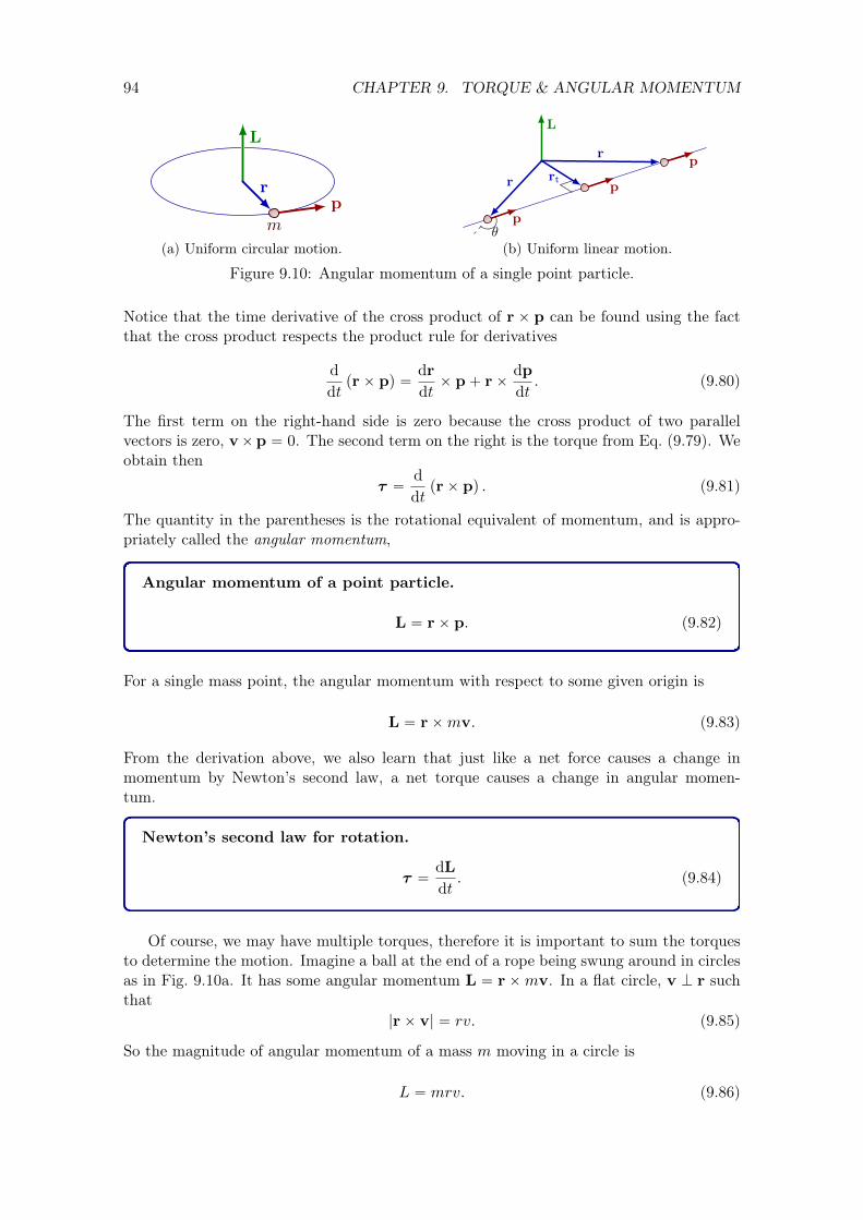
94 CHAPTER 9. TORQUE & ANGULAR MOMENTUM
p
m
L
r
(a) Uniform circular motion.
L
p
p
p
r rt
r
θ
(b) Uniform linear motion.
Figure 9.10: Angular momentum of a single point particle.
Notice that the time derivative of the cross product of r ˆ p can be found using the factthat the cross product respects the product rule for derivatives
d
dtprˆ pq “
dr
dtˆ p` rˆ
dp
dt. (9.80)
The first term on the right-hand side is zero because the cross product of two parallelvectors is zero, vˆp “ 0. The second term on the right is the torque from Eq. (9.79). Weobtain then
τ “d
dtprˆ pq . (9.81)
The quantity in the parentheses is the rotational equivalent of momentum, and is appro-priately called the angular momentum,
Angular momentum of a point particle.
L “ rˆ p. (9.82)
For a single mass point, the angular momentum with respect to some given origin is
L “ rˆmv. (9.83)
From the derivation above, we also learn that just like a net force causes a change inmomentum by Newton’s second law, a net torque causes a change in angular momen-tum.
Newton’s second law for rotation.
τ “dL
dt. (9.84)
Of course, we may have multiple torques, therefore it is important to sum the torquesto determine the motion. Imagine a ball at the end of a rope being swung around in circlesas in Fig. 9.10a. It has some angular momentum L “ rˆmv. In a flat circle, v K r suchthat
|rˆ v| “ rv. (9.85)
So the magnitude of angular momentum of a mass m moving in a circle is
L “ mrv. (9.86)

9.6. ANGULAR MOMENTUM 95
Because v “ rω,
L “ mr2ω. (9.87)
We can plug in the moment of inertia I “ mr2, and find
L “ Iω. (9.88)
More generally, for a rotation we can write it as a vector
Angular momentum.L “ Iω. (9.89)
The ω and thus L follow the right-hand rule in Fig. 9.2. Notice that this equation looksvery similar to p “ mv. This is consistent with our earlier result,
τ “dL
dt“ Iα. (9.90)
9.6.1 Conservation of angular momentum
If there are no external torques, then there is no angular acceleration, and angular mo-mentum is conserved:
0 “dL
dt“ Iα, (9.91)
, similar to the case of p, and
Law of conservation of angular momentum.
pLqbefore “ pLqafter. (9.92)
A well-known example is a figure skater who spins faster after pulling her arms in. Withthe arms closer to the body, her moment of inertia I is smaller, and the angular velocityω has to increase to compensate and keep the angular momentum L stay constant,
pIωqbefore “ pIωqafter. (9.93)
Example: Neutron star
Another cool example are neutron stars, which are known for being extremely dense, andspinning incredibly fast. When a supergiant star of about 10 to 25 solar massesMd reachesits end, it explodes in a supernova and only leaves behind its core which collapses underits own gravity. The neutron star is this collapsed core with a typical mass of 1.4Md,crunched into amazingly small radius of Rns “ 10 km. Say the core initially had a radiusof Rcore “ 8000 km, by what factor will the rotation frequency increase when the core iscompressed into a neutron star of radius Rns “ 10 km and the same mass? For simplicity,suppose that the core and neutron star are homogeneous, solid spheres, then we can use

96 CHAPTER 9. TORQUE & ANGULAR MOMENTUM
Eq. (9.49), such that their moment of inertia I “ 2MR2{5 depends on R2. The frequencyof rotation of the neutron star will be
fns “Icore
Insfcore
“R2
core
R2ns
fcore “ 1ˆ 106fcore.
(9.94)
(9.95)
So if the core was originally spinning with a period of Tcore “ 1000 s, then the neutron starwill spin with a period of Tns “ 1.6 ms, or 640 full revolutions every second! This is indeeda typical period of a neutron star.
Example: Particle moving in a straight line
A particle moving in a straight line has an angular momentum relative to some point noton the line, even though it does not “rotate” around that point. In this case, the positionvector r would be changing, so
L “ rmv sin θ. (9.96)
Clearly, L “ 0 is everywhere with respect to a point on the line because the angle θ “ 0 orπ. The point with respect to which L is defined, is called the point of closest approach. Thelever arm rt points to this point and is perpendicular to the particle’s trajectory. Lookingat the left triangle in Fig. 9.10b, we see that r “ rt{ sin θ, and so in any point r on thepath,
L “ rtmv. (9.97)
This is clearly constant everywhere on the path, which is consistent with conservation ofangular momentum.
9.7 Precession
Suppose you place a disk on a pivot by one of its handles as in Fig. 9.11. If the wheel doesnot spin, the wheel will simply fall over because there is an unbalanced torque of τ “ rmg.But if we spin the wheel with an angular velocity ω, there is still the same torque, howeverthis time, there is an angular momentum L along the axis of the disks rotation. L changesin the direction of τ .
dL “ τdt “ rMg dt τ . (9.98)
FN
mg
(a) The handle allows thedisk to spin around its axisand around the pivot.
α
r
Mg
FN
τ
L = 0
(b) The disk does not spin,and it will fall down due toan unbalanced torque τ .
Lr
Mg
FN
τ
(c) The disk spins, creating anangular momentum L. Torqueτ will cause a precession.
dL
L
τωp
dθ
(d) Torque τ perpendicularto angular momentum L, willonly change its direction.
Figure 9.11: A disk with mass M is placed on a pivot with one of its handles. If the diskspins with angular velocity ω, then it will have an angular momentum L. A torque willcause the angular momentum to change, leading to the phenomenon known as precession.Precession occurs with angular velocity ωp, and the wheel does not fall down.

9.8. ROLLING 97
Because L and τ are perpendicular, the magnitude of L stays constant, and only it’sdirection changes. The wheel does not fall down counter to intuition, but rotates aroundthe pivot. This is called precession.
If we look from above as in Fig. 9.11d, we can see that as the axis of rotation changesby some angle dθ, so does the L vector change by the vector dL.
dL “ Ldθ. (9.99)
We find
dθ “dL
L“rMgdt
L, (9.100)
or,
ωp ”dθ
dt“rMg
L, (9.101)
which is how fast L goes around the pivot. If the wheel is spinning with an angular velocityω, then the angular momentum can be expressed as L “ Iω. Therefore, we can express thefrequency of precession as a function of some constants to do with the mass, radius, gravity,and rotational inertia, as well as an angular velocity ω, which is variable.
Precession.ωp “
rMg
Iω. (9.102)
From this, we see that as ω gets smaller, ωp gets bigger.Precession appears in toy spinning tops and gyroscopes, but Earth also describes a
precession. The Earth rotates about once around its own axis per day, and fully precessesonce every 25 772 years.
9.8 Rolling
Consider a cylinder rolling over a flat surface as in Fig. 9.12a. Say it traveled some distances. If the cylinder was rolling without slipping, it simultaneously rotated by an angle θ thatis related to the distance as
s “ Rθ, (9.103)
because it should be the same as the arc length. The velocity of the center of mass thenhas to be the time-derivative
v “ds
dt“ R
dθ
dt. (9.104)
This gives us the condition
Condition of rolling without slipping.
v “ rω (9.105)
So without slipping, any rolling object with mass M and moment of inertia I has a totalkinetic energy

98 CHAPTER 9. TORQUE & ANGULAR MOMENTUM
Rv
M ω
vθ
s = Rθ
(a) Condition for rolling without slipping is that the lineardistanced s equals the arc length (thick dark blue) of therotated angle θ.
M
θh
(b) A cylinder is released from rest offa ramp. To compute its final velocity,we simply need energy conservation.
Figure 9.12: Cylinder rolling without slipping.
Kinetic energy of a rolling object.
K “1
2Mv2 `
1
2Iω2. (9.106)
The first term is due to its linear motion, and the second due to its rotation.
9.8.1 Example: Rolling off a ramp
Consider a cylinder with radius R and mass M that is let go from a ramp. How fast will itmove at the bottom of a ramp with inclination θ, if it starts from rest at a height h? Wecan now easily solve this with energy conservation. At the top, the cylinder has a potentialenergy mgh, and at the bottom it only has kinetic energy,
Mgh “1
2Mv2 `
1
2Iω2. (9.107)
We know that I “MR2{2 for a solid cylinder and ω “ v{r for rolling without slipping, sothe last equation becomes
Mgh “1
2Mv2 `
M
4v2. (9.108)
and we find
v “
c
4
3gh. (9.109)
If we instead roll a hollow cylinder of the same mass, we need to plug I “ MR2 intoEq. (9.107), and find
v “a
gh. (9.110)
So the hollow cylinder will roll down slower, which is to be expected as it has larger momentof inertia.
9.9 Stability
Mechanical equilibrium is when all forces balance. Consider for example a ball than sitson top of a round hill. The normal force FN balances the ball’s weight mg, but thesmallest sideways push can cause it to roll down the hill. This is therefore called anunstable equilibrium. On the other hand, if the ball sits in a valley or trough, a smallpush will always cause it to be pulled back to its point equilibrium. This is called astable equilibrium. In physics this is often thought of in terms of energy potentials, as inFig. 9.13a. The “valley” is called a potential well, and returns in the study of planetaryattraction, but also nuclear attraction.

9.9. STABILITY 99
U
x
metastable
unstable
stable
(a) A ball on a hill.
U = mgh
φ−90° 90°0°
mgH/2
mgW/2
metastable metastable
unstableunstable
stable
(b) A rectangular block with widthW and heightH (Fig. 9.16).
Figure 9.13: Potential wells with stable, metastable and unstable equilibria.
Some potentials might have another local minimum elsewhere (like a lake on a moun-tain), where the ball can sit stably. However, if the push is large enough, it can causethe ball to roll over a local maximum, and drop into an even lower minimum. This iscalled a metastable equilibrium. The amount of energy to get it over the “barrier” is calledactivation energy, which is a useful concept in chemistry. Namely, you have to pay somesmall activation energy to let the ball release a big amount of, often useful, energy. In caseof a ball in a local minimum of a hill, the activation energy is E “ mg∆y, where ∆y is theheight difference with the barrier.
Lastly, if a ball sits on a completely flat surface, it is in a neutral equilibrium. The balldoes not restore itself to its original position if you give it a small push (like in a stableequilibrium), but it also does spontaneously gain energy (unstable equilibrium).
But we also have seen rotational equilibrium in Section 9.3. In this case there will beno angular acceleration, because all torques cancel. If both the sum of forces and the sumof torques are zero, you have a static equilibrium.
Static equilibrium.$
&
%
ÿ
Fi “ 0ÿ
τ i “ 0
(9.111)
(9.112)
If the body starts from rest, the first equation implies that the center of mass will not havea linear motion, and the second equation says that there will not be rotation.
We have already seen one example in the seesaw Fig. 9.5 and in precession of the diskFig. 9.11, let’s look at some other real life ones.
y
x
+
Ff
FN Mg
FW
θ
π
2− θ
π − θ
(a) Without a person.
Ff
FN Mg
FW
mgr
θ
(b) With a person of mass m,there is an extra weight.
Ff
FN
(m+M)g
FW
r
θ
(c) Alternative to (b), take the ladder-person as one system, shifting the CM.
Figure 9.14: Ladder of length L leaning against a wall. There is the weight, friction, normalforce from the ground, and normal force from the wall. We assume no friction on the wall.
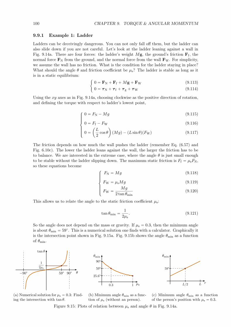
100 CHAPTER 9. TORQUE & ANGULAR MOMENTUM
9.9.1 Example 1: Ladder
Ladders can be deceivingly dangerous. You can not only fall off them, but the ladder canalso slide down if you are not careful. Let’s look at the ladder leaning against a wall inFig. 9.14a. There are four forces: the ladder’s weight Mg, the ground’s friction Ff , thenormal force FN from the ground, and the normal force from the wall FW. For simplicity,we assume the wall has no friction. What is the condition for the ladder staying in place?What should the angle θ and friction coefficient be µs? The ladder is stable as long as itis in a static equilibrium:
#
0 “ FN ` Ff `Mg ` FW
0 “ τN ` τ f ` τ g ` τW
(9.113)(9.114)
Using the xy axes as in Fig. 9.14a, choosing clockwise as the positive direction of rotation,and defining the torque with respect to ladder’s lowest point,
$
’
’
’
’
&
’
’
’
’
%
0 “ FN ´Mg
0 “ Ff ´ FW
0 “
ˆ
L
2cos θ
˙
pMgq ´ pL sin θqpFWq
(9.115)
(9.116)
(9.117)
The friction depends on how much the wall pushes the ladder (remember Eq. (6.57) andFig. 6.10c). The lower the ladder leans against the wall, the larger the friction has to beto balance. We are interested in the extreme case, where the angle θ is just small enoughto be stable without the ladder slipping down. The maximum static friction is Ff “ µsFN,so these equations become
$
’
’
’
’
&
’
’
’
’
%
FN “Mg
FW “ µsMg
FW “Mg
2 tan θmin
(9.118)
(9.119)
(9.120)
This allows us to relate the angle to the static friction coefficient µs:
tan θmin “1
2µs. (9.121)
So the angle does not depend on the mass or gravity. If µs “ 0.3, then the minimum angleis about θmin “ 59˝. This is a numerical solution one finds with a calculator. Graphically itis the intersection point shown in Fig. 9.15a. Fig. 9.15b shows the angle θmin as a functionof θmin.
tan θ
θ−90° 90°59°
1
2µs
(a) Numerical solution for µs “ 0.3: Find-ing the intersection with tan θ.
θmin
µs10.3
90°
59°
25.6°
(b) Minimum angle θmin as a func-tion of µs (without an person).
θmin
rL/2 L
59°
(c) Minimum angle θmin as a functionof the person’s position with µs “ 0.3.
Figure 9.15: Plots of relation between µs and angle θ in Fig. 9.14a.

9.9. STABILITY 101
But what if a person of mass m starts climbing the ladder? The new condition forstatic equilibrium is
$
’
’
’
’
&
’
’
’
’
%
0 “ FN ´Mg ´mg
0 “ Ff ´ FW
0 “ pr cos θminq pmgq `
ˆ
L
2cos θmin
˙
pMgq ´ pL sin θminqpFWq
(9.122)
(9.123)
(9.124)
where r is the position of the person on the ladder, r “ 0 being on the bottom, r “ L ontop. This time, the solution is given by
tan θmin “rm` LM{2
µspm`MqL. (9.125)
A special case is when the person stands in the middle of the ladder, r “ L{2, and weagain find that tan θmin “ 1{2µs. This means that in this case, it is as if there is noperson. What if the person stand lower or higher? Because Eq. (9.125) increases with r, asshown in Fig. 9.15c, and because tan is a monotonously increasing function, it follows thatthe minimum angle θmin is larger if x ą L{2 (tan θmin ą 1{2µs), and smaller if x ă L{2(tan θmin ă 1{2µs). So, if the ladder were set at the minimum angle without a person, andthen a person walks up the ladder, after they pass the mid-point, the ladder would becomeunstable and fall !
9.9.2 Example 2: Rectangular block
Consider the rectangular block with width W , height H and homogeneous mass m inFig. 9.16. Intuitively, we know that the block is more stable if it rests on its long side thanits short one. Why?
Say the block rests on its short side as in Fig. 9.16a. Then all torques will balance,
pr sin θqmg ´ rtFN “ 0, (9.126)
because FN “ mg and rt “ r sin θ. This is a metastable state, because a small pushwill manage to not topple it and cause the block to return to this equilibrium position.However, if the push is large enough it will fall over to a more stable position on its longside.
Say you pivot the block just a little bit as in Fig. 9.16b over its right corner, but withthe center of mass on the left side of the pivot point. If you let it go from rest, there willbe an unbalanced, restoring torque due to gravity, τ “ rˆmg.
W
H
θmg
FN τ = 0
r
rt
(a) Metastable equilibrium:Standing on short side. Alarge push can topple it.
mg
FN
τ
r
α
(b) No equilibrium: thereis an unbalanced nonzerotorque.
mg
FN
τ = 0
φ
(c) Unstable equilibrium:The center of mass is rightabove the pivot point.
mgmg FN
τ = 0
(d) Stable equilibrium: Ly-ing on it long side. It takesmore energy to pivot it.
Figure 9.16: Stability of a rectangular block of width W , height H and mass m.

102 CHAPTER 9. TORQUE & ANGULAR MOMENTUM
CM
(a) Balancing witharms, to increase themoment of inertia.
CM
(b) Balancing with long rod to in-crease moment of inertia even more,and slightly lower the center of mass.
CM
(c) Stabilize by lower-ing the center of massbelow the rope.
CM
FN
mg
τr
θ
(d) Restoring torquewhen the center of massis below the pivot point.
Figure 9.17: Tightrope artist walks on a rope.
But what if you balance it just right, such that the center of mass is exactly abovethe pivot point? Now, the torque due to gravity vanishes, because it is antiparallel to theposition vector, and thus rˆmg “ 0. This is an unstable equilibrium, because the smallestpushes in will cause it to fall. This is why it is hard to balance a pencil on its tip.
This can be expressed in terms of potential wells, by realizing that the block has amaximum gravitational energy U “ mgh (with h ą H{2) when it is balance on one of itscorners. When it rests on its short side, it has a lower potential energy (U “ mgH{2),because the center of mass is lower, and when it is on its long side even lower (U “ mgW {2).This is plotted in Fig. 9.13b.
9.9.3 Example 3: Tightrope artist
Walking on a tightrope is a classic example of a balancing act. Without any help, thecenter of mass of a tightrope artist is above the pivot point, meaning that any small pushcan cause her to tip over. By extending the arms, the artist can increases her moment ofinertia and make small adjustments. By carrying a rod as in Fig. 9.17b, she increases themoment of inertia event more, and has more control over it. A bent rod will also lowerthe center of mass, making her more stable. But to become fully stable, one can “cheat”by carrying heavy weights that lower the center of mass to below the rope, as shown inFig. 9.17c. Any small rotation will be counteracted by a restoring torque pulling the centerof mass back to below the pivot point, Fig. 9.17d. This is how self-balancing toys work.
9.10 Summary
We have seen many formulas for rotational motion in this chapter. Luckily they are closelyrelated to linear motion, and there is a lot of concepts and formulas that are similar. Theyare summarized and compared in Table 9.1. Make sure you understand in what case theseformulas can be applied and in which cases they cannot.

9.10. SUMMARY 103
Table 9.1: Comparison of linear and rotational formulas.
Name Linear RotationalPosition x “ x0 ` v0t`
12at
2 θ “ θ0 ` ω0t`12αt
2
Velocity v “ v0 ` at ω “ ω0t` αt
Acceleration a α
Inertia m I “ş
r2dm
Force F τ “ rˆ F
Momentum p “ mv L “ rˆ p “ Iω
Newton’s second lawÿ
F “dp
dt“ ma
ÿ
τ “dL
dt“ Iα
Work W “ F ¨∆x W “ τ∆θ
Kinetic energy K “ 12mv
2 K “ 12Iω
2
Power P “ F ¨ v P “ τω
Momentum conservationř
pi “ř
pfř
Li “ř
Lf
Equilibriumř
F “ 0ř
τ “ 0

104 CHAPTER 9. TORQUE & ANGULAR MOMENTUM

Chapter 10
Non-inertial reference frames &Pseudo Forces
10.1 Inertial reference frames
In Section 8.4 we saw the Galilean coordinate transformation Eq. (8.52) between tworeference frames that move with a uniform velocity with respect to each other. Twoobservers in each of these reference frames will see different things happen, but the physicalprediction stays the same. All you need to do is transform the coordinates.
Take for example, Alice in frame S, who is standing at rest with respect to the ground,and Bob in frame S1, who is in a car moving with constant velocity v with respect to Aliceand frame S. Alice sees Bob moving away with a velocity v, and Bob, who thinks he is atrest, sees Alice moving away from him with a velocity v. When Alice throws up a ball, itwill follow a one-dimensional vertically path according to
$
&
%
xptq “ 0
yptq “ v0yt´gt2
2
(10.1)
(10.2)
When Bob throws up his own ball with the same initial velocity v0y, he will see it followa one-dimensional path in his own frame as well. He will describe it with
$
’
&
’
%
x1ptq “ 0
y1ptq “ v0yt´gt2
2
(10.3)
(10.4)
S
y
x
S′
y′
x′v S′
y′
x′v
Figure 10.1: Throwing a ball in two inertial reference frames S and S1 moving at a relativevelocity v. Alice in S sees Bob’s ball moving in a parabolic trajectory, while Bob sees hisball moving only vertically.
105

106 CHAPTER 10. NON-INERTIAL REFERENCE FRAMES & PSEUDO FORCES
However, Alice in S will see Bob’s ball form a parabolic path as in Fig. 10.1. Alice can useGalilean transformation to move Eqs. (10.3) and (10.4) to her own coordinate system:
$
’
&
’
%
xptq “ x1ptq ` vt “ vt
yptq “ y1ptq “ v0yt´gt2
2
(10.5)
(10.6)
which is indeed a parabola. From Bob’s perspective in S1, Alice’s ball will also follow aparabola, but in the negative x1 direction. Even though they arrive at different descriptions,the physics (i.e. gravity) is the same, and their results are related by a simple coordinatetransformation.
10.2 Non-inertial reference frames
But what if a frame is accelerated with respect to another one? Consider again Alice inframe S and Bob in frame S1, but this time Bob’s car is sped up with a uniform accelerationa. Say there is a mass m suspended from the car’s ceiling by a wire, which was initially atrest. The mass m has some inertia, so once the car starts moving, the wire pulls the massalong with a tension T. This causes the mass and wire to deflect with an angle θ as shownin Fig. 10.2a. Newton’s second law says
ma “ mg `T, (10.7)
where the horizontal component of the tension causes an acceleration a, as illustrated inFig. 10.2b. But this is in Alice’s frame S, which is at rest. Bob, however, thinks he andthe mass are the ones at rest and sees a mysterious force F1 pulling the mass:
0 “ mg `T` F1. (10.8)
The mass is at equilibrium in S1. So clearly, this new force is given by the acceleration,
F1 “ ´ma. (10.9)
In fact, Bob will also feel this force F1 and might fall over if he is not careful. This is a so-called pseudo-force, or also a fictitious or inertial force. Because masses have inertia, pseudoforces like F1 or the centrifugal force mentioned in Section 6.7 will appear in acceleratedframes like S1. A frame that does not have pseudo forces is called an inertial frame ofreference.
Inertial frame of reference. In an inertial frame of reference, all bodies with azero net force acting upon them do not accelerate.
a
θ
mS′
y′
x′
(a) Bob in non-inertial frame S1 is con-fused about the mass deflecting.
Ty
Tx
T
mg
maθ
S
(b) Force balance in iner-tial frame S.
Ty
Tx
T
mg
F ′θ
S′
(c) Force balance in Bob’snon-inertial frame S1.
Figure 10.2: When Bob’s car accelerates, the mass suspended from the ceiling seems toexperience a force F1 in accelerated frame S1.

10.2. NON-INERTIAL REFERENCE FRAMES 107
This is actually one of the reasons why Newton wisely included the first law, which mightseem redundant as a special case of the second law (F “ 0 such that a “ 0). By includingthe first law in addition to the second law, one can postulate that only (real) forces inan inertial reference frame can accelerate masses, otherwise a mass will stay at rest ormove in a straight line with constant speed. Equivalently, you can define inertial framesof reference as those reference frames in which Newton laws hold true.
Note that any frame moving with a constant vcm with respect to an inertial lab frame,is also an inertial frame of reference.
A non-inertial reference frame then, is a(n accelerated) frame where pseudo forces ariseand Newton’s law are violated. Some typical examples are a passenger in a car that is goingaround the bend (centripetal acceleration), an astronaut being launched in a rocket, or askydiver in free fall (before hitting terminal velocity).
The perceived force due to acceleration is often expressed in units of gravitational forceequivalent, or g-force. For example, the driver in a fast race car that accelerates by a “ gwill feel a g-force of “3 g”, which is the force the seat pushes back on them. A Space Shuttlelaunch or reentry is typicall 1 g, and the highest g-force on a roller coaster (in 2020) is upto a whopping 6.3 g on the Tower of Terror in at Gold Reef City in Gauteng, South Africa.
We typically assume a lab frame at rest on the earth’s surface is an inertial. However,this is not strictly true due to the Earth’s rotation. A section below will explore theCoriolis effect among others, which cause a ball that is dropped to the ground to notfollow an exactly straight path, seemingly violating Newton’s first law until the rotationsare considered.
10.2.1 Coordinate transformation
The physical prediction between two frames that are accelerated with respect to each otheris different, because an observer in one frame will claim there is an acceleration, while theother will claim there is a force. The coordinate transformation becomes
Coordinate transformation to an accelerated frame.
r1 “ r´aframet
2
2, (10.10)
where frame S1 is moving with a uniform acceleration vframe with respect to frame S, andhas no initial velocity. For simplicity, take the initial velocity and acceleration between theframes to be only in the x direction, in which case the coordinates of the position vectorr1 in the accelerated S1 frame are given by
$
’
’
’
&
’
’
’
%
x1 “ x´aframet
2
2y1 “ y
z1 “ z
(10.11)
(10.12)(10.13)
Notice that from Bob’s perspective in S1, Alice is actually the one that is accelerated by´aframe.

108 CHAPTER 10. NON-INERTIAL REFERENCE FRAMES & PSEUDO FORCES
S
z
yx
T
am
ω
ω
(a) Alice in inertial frame S sees that the mass ex-periences a centripetal force from tension T.
T Fcf
m
S′z′
y′x′
(b) Bob in non-inertial frame S1 sees that the massexperiences a centrifugal force creating a tension T.
Figure 10.3: A rotational frame gives rise to the fictious centrigual force. Mass m rotateswith a merry-go-around (red disk) and is radially held in place by a wire with tension T.
10.3 Rotational frames
10.3.1 Centrifugal force
Now consider a uniformly rotating frame as in Fig. 10.3. Alice looks from the side ininertial frame S, while Bob is on the rotating merry-go-around in rotating frame S1. Amass is suspended to the middle by a wire and rotates in circles with the merry-go-around.To hold the mass radially in place, the wire provides a centripetal force with its tension T,
ma “ T. (10.14)
Meanwhile, Bob scratches his head because he notices there is a mysterious centrifugalforce creating a tension in the wire:
0 “ T` Fcf . (10.15)
Again, the mass is at equilibrium in S1 and the forces balance. Comparing the latter twoequations,
Centrifugal force. The centrifugal force is opposite to the centripetal acceleration
Fcf “ ´ma “mv2
rr. (10.16)
where we assumed the centripetal acceleration in frame S points to the origin on rotationaxis, just as in Eq. (5.35).
10.3.2 Extra: Coordinate transformation of rotation
This section is extra, for interested people, but is not part of the main curriculum. Someknowledge of matrices and their properties is assumed.
So what is the coordinate transformation between S and S1? Suppose the coordinatesystems of the two frame have the same origin, and S1 rotates counterclockwise with auniform angular velocity ω, as in Fig. 10.4a. A point P that has coordinates px, yq in S,will have coordinates
#
x1 “ x cospωtq ` y sinpωtq
y1 “ ´x sinpωtq ` y cospωtq
(10.17)(10.18)

10.3. ROTATIONAL FRAMES 109
P
xO
y
x′
y′
r
θ = ωt
(a) A point or position vector r has different co-ordinates in the S and S1 frame.
P
xO
y
x′
y′
θ
θ
θ
θx
y
x cos θ
y sin θ
y sin θ
xsinθ
xsinθ
ycos
θ
(b) The coordinate transformation px, yq ÞÑ px1, y1q canbe derived by finding the right triangles and angles.
Figure 10.4: Frame S’ is rotated counterclockwise with a time-dependent angle θ “ ωtwith respect to frame S.
in frame S1, as can be gleaned from Fig. 10.4b. In terms of linear algebra, this correspondsto the linear transformation
ˆ
x1
y1
˙
“
ˆ
cospωtq sinpωtq´ sinpωtq cospωtq
˙
¨
ˆ
xy
˙
(10.19)
where the matrix Rpωtq is the clockwise-rotation matrix with rotation angle θ “ ωt
Rpθq “
ˆ
cos θ sin θ´ sin θ cos θ
˙
(10.20)
This matrix has the nice property that its transpose is its inverse:
R´1pθq “ RTpθq “ Rp´θq. (10.21)
In linear algebra, matrices with this property are called orthogonal. It implies that itpreserves the length in the scalar product after transformation, and therefore any lengths:
r1 ¨ r1 “ r ¨ r. (10.22)
Notice that with the above choice of coordinate systems, the position vectors r1 “ rare identical because the origins coincide,
r1 “ x1x1 ` y1y1 ` z1z1
“ xx` yy ` zz “ r.
(10.23)(10.24)
The unit vectors in S1 are given by
x1 “ cospωtqx` sinpωtqy
y1 “ ´ sinpωtqx` cospωtqy
z1 “ z.
(10.25)(10.26)(10.27)
The unit vectors x, y and z are constant with time in S, but the ones from S1 change withtime in S as
dx1
dt“ ´ω sinpωtqx` ω cospωtqy
dy1
dt“ ´ω cospωtqx´ ω sinpωtqy
dz1
dt“ 0.
(10.28)
(10.29)
(10.30)

110 CHAPTER 10. NON-INERTIAL REFERENCE FRAMES & PSEUDO FORCES
Because the rotation assumed to be counterclockwise in Fig. 10.4a, the constant angularfrequency vector is ω “ ωz. So we can rewrite the above time-derivatives as
dx1
dt“ ω ˆ x1
dy1
dt“ ω ˆ y1,
(10.31)
(10.32)
such that the derivatives are orthogonal to ω and the corresponding unit vector. It turnsout that this holds more generally for any choice of direction of ω,
dx1
dt“ ω ˆ x1,
dy1
dt“ ω ˆ y1,
dz1
dt“ ω ˆ z1. (10.33)
So the change in direction of these unit vector is always perpendicular to the rotation axisand to the given unit vector itself, so its size is constant, as expected. In other words, thechange is tangential. Clearly, if a unit vector is parallel to the rotation axis ω, it will notchange direction (e.g. x1 ‖ ω ñ ω ˆ x1 “ 0). On the other hand, the change of directionwill be maximal if the unit vector is perpendicular to ω (e.g. x1 K ω ñ |ω ˆ x1| “ ω).
10.3.3 Extra: Time derivation of a vector function
This section provides some mathematical formulas to help derive the pseudo-forces observedin a rotating frame.
Take any time-dependent vector function A in inertial frame S,
A “ Axx`Ayy `Azz. (10.34)
This vector can be anything, including the position r. The time derivative of A is givenby the derivative of its coordinates in S
dA
dt
ˇ
ˇ
ˇ
ˇ
S
“dAxdt
x`dAydt
y `dAzdt
z, (10.35)
because the unit vectors are constant in time in frame S. Now look at the same vector,but with expressed in coordinates of a rotating frame S1,
A “ A1xx1 `A1yy
1 `A1zz1, (10.36)
where the coordinates and unit vectors are defined in S1. The time derivative of A in S,with S1 coordinate system is
dA
dt
ˇ
ˇ
ˇ
ˇ
S
“
ˆ
dA1xdt
x1 `dA1ydt
y1 `dA1zdt
z1˙
`
ˆ
A1xdx1
dt`A1y
dy1
dt`A1z
dz1
dt
˙
(10.37)
due to the product rule. The terms between the first parenthesis in Eq. (10.37) is thechange of A in non-inertial frame S1, wherein the unit vectors x1, y1 and z1 are constant.Therefore, Eq. (10.37) becomes
dA
dt
ˇ
ˇ
ˇ
ˇ
S
“dA
dt
ˇ
ˇ
ˇ
ˇ
S1
` ω ˆ`
A1xx1 `A1yy
1 `A1zz1˘
, (10.38)
where we also substituted Eq. (10.33). So using Eq. (10.36), we find the following usefulresult.

10.3. ROTATIONAL FRAMES 111
Kinematic transport theorem.
dA
dt
ˇ
ˇ
ˇ
ˇ
S
“dA
dt
ˇ
ˇ
ˇ
ˇ
S1
` ω ˆA. (10.39)
So the change of A in frame S is related to its change relative to the rotating frame S1 bysimply adding the term ω ˆA tangentially to A.
10.3.4 Pseudo forces in a rotating system
The centrifugal force is not the only pseudo force that appears in a rotating system. We willnow formally derive the other two that arise starting from the transport theorem (10.39)and deriving a relation between the acceleration in inertial reference frame S and rotatingreference frame S1 to see if extra terms show up that indicate the presence of pseudo forces.
In Eq. (10.39), A can be any vector. For example, the position vector A “ r “ r1,
dr
dt
ˇ
ˇ
ˇ
ˇ
S
“dr
dt
ˇ
ˇ
ˇ
ˇ
S1
` ω ˆ r, (10.40)
These are the velocities v in the S frame, and v1 in the S1 frame
v “ v1 ` ω ˆ r, (10.41)
where ω ˆ r encodes the tangential velocity from the rotation ω. By deriving expres-sion (10.40) with respect to time, we find the acceleration a in frame S,
a “d2r
dt2
ˇ
ˇ
ˇ
ˇ
S
“d
dt
ˆ
dr
dt
ˇ
ˇ
ˇ
ˇ
S1
` ω ˆ r
˙
. (10.42)
Following the product rule,
a “d
dt
ˆ
dr
dt
ˇ
ˇ
ˇ
ˇ
S1
˙
`dω
dtˆ r` ω ˆ
dr
dt(10.43)
We can apply the transport theorem (10.39) to r in the last term, which is Eq. (10.40),and to the vector between the parentheses in the first term, which is
d
dt
ˆ
dr
dt
ˇ
ˇ
ˇ
ˇ
S1
˙
“d2r
dt2
ˇ
ˇ
ˇ
ˇ
S1
` ω ˆdr
dt
ˇ
ˇ
ˇ
ˇ
S1
. (10.44)
Putting everything together,
a “d2r
dt2
ˇ
ˇ
ˇ
ˇ
S1
` 2ω ˆdr
dt
ˇ
ˇ
ˇ
ˇ
S1
` ω ˆ pω ˆ rq `dω
dtˆ r. (10.45)
Because the position vector r “ r1 in case of rotation in the same origin, we can define thevelocity and acceleration measured in frame S1 as
v1 “dr
dt
ˇ
ˇ
ˇ
ˇ
S1
, a1 “d2r
dt2
ˇ
ˇ
ˇ
ˇ
S1
, (10.46)
and write the result as
112 CHAPTER 10. NON-INERTIAL REFERENCE FRAMES & PSEUDO FORCES
Acceleration in rotating frame.
a “ a1 ` 2ω ˆ v1 ` ωpˆω ˆ r1q `dω
dtˆ r1. (10.47)
We see that indeed extra terms pop up in the acceleration a1 in the S1 frame. This shouldgive us a hint of new pseudo forces! This is easy to see if you first invoke Newton’s secondlaw in the inertial frame S,
ma “ÿ
F, (10.48)
whereř
F is the total force observed in inertial frame S. After substituting Eq. (10.47),we see that in the rotating frame S1
Newton’s second law in a rotating system.
ma1 “ÿ
Floomoon
real
´ 2mω ˆ v1loooooomoooooon
Coriolis
´mω ˆ pω ˆ r1qloooooooooomoooooooooon
centrifugal
´mdω
dtˆ r1
loooooomoooooon
Euler
. (10.49)
These are three extra pseudo forces observed in the rotating system S1.
Pseudo forces in a rotating system.
• The Coriolis force FCor “ ´2mω ˆ v1 appears when the particle is moving inthe S1 (v1 ‰ 0).
• The centrifugal force Fcf “ ´mωˆpωˆr1q appears if the particle is at a nonzerodistance from the rotational axis (r1 ‰ 0).
• The Euler force FEul “ ´mdω
dtˆr1 appears when the reference frame experiences
an angular acceleration (dω {dt ‰ 0).
Notice that if ω K r1, that the centrifugal force points again in the radial direction,
Fcf “ ´mω ˆ pω ˆ r1q “ mω2rr1, (10.50)
because ω ˆ pω ˆ rq “ ´r.
10.3.5 Coriolis force
Let’s focus on the Coriolis force
FCor “ ´2mω ˆ v1. (10.51)
This force is perpendicular to the rotation ω and the velocity v1 in the rotating frame S1.It is also proportional to the angular frequency ω and speed v1.
Suppose that the velocity moves in the rotation plane, i.e. v1 K ω and take ω “ ωz,then the Coriolis force for a velocity v1 “ v1xx
1 ` v1yy1 is
FCor “ 2mωpv1yx1 ´ v1xy
1q. (10.52)

10.3. ROTATIONAL FRAMES 113
This is a bit hard to interpret, so let’s break down v1 into polar coordinates in the x1y1
plane of the inertial frame S1,
v1 “ v1rr` v1θθ, (10.53)
where r1 “ r and θ1“ θ between S and S1. In this case, the Coriolis force is given by
FCor “ ´2mω ˆ pv1rr` v1θθq. (10.54)
Because zˆ r “ θ and zˆ θ “ ´r,
FCor “ 2mωpv1θr´ v1rθq. (10.55)
10.3.6 Example: Throwing a ball on rotating disk
Suppose Alice stands in the middle of a large rotating disk and throws a ball to Bobstanding at the disk’s edge. When she throws the ball at t “ 0, it will follow a straightpath in the inertial frame S to where Bob was at t “ 0, if the ball moves along the y axis,
rptq “ vty. (10.56)
By the time the ball reaches the edge, Bob has already rotated away as in Fig. 10.5a. Fromthe perspective of Alice and Bob in the rotating frame S1, the ball follows a curved path asin Fig. 10.5b. In S1, the ball seems to experience a mysterious force, namely the Coriolisforce! The coordinates of rptq in S1 are given by
r1ptq “ vt sinpωtqx1 ` vt cospωtqy1, (10.57)
or in polar coordinates,
r1ptq “ vtr1 ´ ωtθ1, (10.58)
which describes a clockwise spiral in S1, i.e. a uniform circular motion θ “ ωt, except thatthe radius r “ vt increases with time. The deflection is caused by the Coriolis force FCor,which is perpendicular the v. At the same time there is the centrifugal force Fcf whichseems to radially increase the velocity.
v
m
ω
S
y
x
y′ x′
A
B
(a) Mass m moves in a straight line ininertial frame S.
S′
y′
x′
v
FCor
mS
y
x
y
xω
(b) Mass m moves in a spiral in rotat-ing frame S1.
S′
y′
x′
vFcf
FCorFCor
v
Fcf
FCor
v
Fcf
FCor
(c) The spiral motion in S1 is caused by thecentrifugal and Coriolis force.
Figure 10.5: Alice (A) throws a ball of mass m from the center of a disk to Bob (B) at theedge of the disk. Because its velocity is nonzero in the rotating frame S1, a Coriolis forcewill cause a deflection in the rotating S1.

114 CHAPTER 10. NON-INERTIAL REFERENCE FRAMES & PSEUDO FORCES
10.3.7 Example: A ball at rest
What if the ball simply stays at rest at some radial distance r from the origin in the inertialframe S? Without loss of generality, say its coordinates are given by
rptq “ rx “ rr (10.59)
and v “ 0 in S, andr1ptq “ r cospωtqx1 ` r sinpωtqy1 “ rr1 (10.60)
in the rotating frame S1, meaning the ball appears to rotate clockwise around the origin.The velocity in S1 is given by
v1ptq “ ´rω sinpωtqx1 ` rω cospωtqy1
“ ´rωθ1,
(10.61)
(10.62)
such that it is tangential to the position r, and has size v “ rω, as one would expectfor a uniform circular motion. Note this is also consistent with the transport theoremEq. (10.41) for r. The velocity v1 is nonzero in S1, so there is a Coriolis force (10.55). Inthis case it is in the negative radial direction
FCor “ ´2mω2rr1, (10.63)
while the centrifugal force isFcf “ mω2rr1. (10.64)
Putting this together in the second law in S1,
ma “ FCor ` Fcf “ ´mω2rr1, (10.65)
which is consistent with the centripetal force (5.44) for uniform circular motion.
10.3.8 Example: Centrigufal force on Earth
The Earth spins, and is therefore not an non-inertial reference frame. Assuming the rota-tion is constant over time, there will be a Coriolis and centrifugal force, but no Euler force.Let’s compare the former two depending where you are on Earth. Because of symmetry,the only important piece of information is your latitude θ. Anywhere at the equator,φ “ 0, while at the North Pole it is φ “ 90˝ and at the South Pole it is φ “ ´90˝. Thecentrifugal force only depends on the radial distance r “ R cosφ from the rotation axis,where R « 6370 km is Earth radius. So the centrifugal force is
Fcf “ mω2r “ mω2R cosφ, (10.66)
where ω « 2π{1 day “ 7.27ˆ 10´5 {s. The centrifugal force is zero at the poles, andbiggest at the equator, where for 1 kg
Fcf “ mω2R “ 0.034 N. (10.67)
The centrifugal acceleration that opposes the gravitational field g is
acf “ ω2R “ 0.034m
s. (10.68)

10.3. ROTATIONAL FRAMES 115
In other words, if at the poles weight is measured as simple mg, then the difference inmeasured weight at the equator is
´Fcf
mg“ ´
ω2R
g“ ´0.35% (10.69)
In reality the difference is closer to 0.5%, as the Earth is not a perfect sphere. Due to thecentrifugal force, the Earth is “flattened” a bit, and looks more like oblate spheroid. As aconsequence, the gravity is stronger at the poles, which are closer to Earth’s center (about6378 km) than at the equator (about 6357 km).
10.3.9 Example: Coriolis force on Earth
How does the centrifugal force compare tot the Coriolis force? This force is maximumwhen the velocity is perpendicular to the rotation axis, v1 K ω, when
FCor “ 2mωv (10.70)
So for a 1 kg object moving at an appreciable speed of 100 km{h,
FCor “ 0.0040 N, (10.71)
almost ten times smaller than the centrifugal force for the same mass.Still, the Coriolis effect has a large impact on the directions of things like winds and
ocean currents. In the Northern Hemisphere, a mass moving from west to east will expe-rience a southward deflection, and vice verse, a mass moving from east to west will noticea northward deflection. Similar for longitudinal north-south travel. This will cause windson the Northern Hemisphere to spiral counterclockwise as in Fig. 10.6b. On the Southernhemisphere it will be clockwise instead. Despite what you may have seen on the Simpsons,this effect is not strong enough to determine the sense of a vortex in a kitchen drain oftoilet, as other initial condition can influence the direction.
Interestingly, this effect is also noticeable on the railroad tracks for trains movinglongitudinally: A train moving from north to south in the Northern Hemisphere will putmore force on the west track (right in facing the direction of motion), while a train movingfrom south to north will put more force on the east track (again right). This means thatright tracks in the Northern Hemisphere will tend to wear out faster than the left one. Asimilar effect is seen in the shape of river beds.
Another phenomena that the Coriolis effect influences are jet streams. As hot airmoves from the high to low pressure zones, it tends to be deflected eastward in bothhemispheres, creating jet stream between 9 and 16 km. These jet streams have a largeimpact on flight times. Eastward planes pick up a tail wind and arrive quicker thanwithout, while westbound planes take longer. For example, planes flying from New Yorkto London take roughly seven hours, while the return takes about eight.
ω
rFcf
φ
(a) The centrigufal force on Earth’s surface de-pends on the latitude φ.
N
W
E
S
(b) The Coriolis force depends on which directionyou move.
Figure 10.6: Earth rotates, so pseudo forces arise.

116 CHAPTER 10. NON-INERTIAL REFERENCE FRAMES & PSEUDO FORCES

Part II
Oscillations and Waves
117


Chapter 11
Harmonic oscillations
11.1 Interlude: Taylor expansion
Physicists like to model the physical world by starting with simplifications and approxi-mations. One indispensable mathematical tool for a physicist are Taylor approximations.From analysis, we remember that
Taylor series. The Taylor series of a function f that is infinitely differentiable ina is the power series
fpxq “ fpaq `f 1paq
1!px´ aq `
f2paq
2!px´ aq2 `
f3paq
3!px´ aq3 ` ...
“
8ÿ
n“0
f pnqpaq
n!px´ aqn
(11.1)
(11.2)
Accordingly, the nth Taylor polynomial is the polynomial of degree n,
Tnpxq “nÿ
i“0
f piqpaq
i!px´ aqi. (11.3)
T1 is the tangent line to fpxq at x “ a with slope f 1paq. Typically, the more terms youadd, the better you approximate f around x “ a, fpxq « Tnpxq. Also the closer you stayto x “ a (so small |x´ a|), the smaller the difference Tnpxq ´ fpxq. A special case of aTaylor series is when a “ 0.
Maclaurin series.
fpxq “ fp0q `f 1p0q
1!x`
f2p0q
2!x2 `
f3p0q
3!x3 ` ...
“
8ÿ
n“0
f pnqp0q
n!xn
(11.4)
(11.5)
11.1.1 Example 1: Cubic function
As a simple example, consider a cubic function
fpxq “ x3 ´ x2 ´ x` 1. (11.6)
119

120 CHAPTER 11. HARMONIC OSCILLATIONS
y
x
f
T1
T21
−1
1−1−1
Figure 11.1: First (green) and second (red) degree Taylor polynomials that approximatefpxq “ x3 ´ x2 ´ x` 1. T1 has two lines for x “ 0 and x “ 1, while T2 has two curves.
The first, second and third Taylor polynomials in x “ 0 are
T1pxq “ 1´ x
T2pxq “ 1´ x´ x2
T3pxq “ 1´ x´ x2 ` x3
(11.7)
(11.8)
(11.9)
Notice that with T3pxq we retrieve the original function fpxq, because they are both third-degree polynomial. Similarly, in a different point, x “ 1, they are
T1pxq “ 0
T2pxq “ 2px´ 1q2
T3pxq “ 2px´ 1q2 ` px´ 1q3
(11.10)
(11.11)
(11.12)
Notice that the last result T3pxq is again the exact same as fpxq and Eq. (11.9).
11.1.2 Example 2: Sine
For the purposes of this course, it is important to know the Taylor expansion of sine:
sinx “ x´x3
3!`x5
5!´x7
7!`x9
9!` ...
“
8ÿ
n
p´1qn
p2n` 1q!x2n`1.
(11.13)
(11.14)
The series only has terms of odd degree. Several Taylor polynomials are shown in Fig. 11.2a.The first-order approximation of a sine function is a linear one,
sinx « T1pxq “ x. (11.15)
y
x
sin
T1
T3T5
T7
T9
T−T
(a) Taylor polynomials Tn, see Eq. (11.13).
Tn(x)−sin x|sin x|
x
T9
T7T5
T3
T1
1
−1
180°−180°
(b) Relative difference with Tn.
x
T1(x)− sinx
|sinx|
1%
−1%
2%
−2%
3%
−3%
10°−10° 20°−20°
(c) Relative difference with T1.
Figure 11.2: Taylor expansion approximating sine fpxq “ sinx. The first-order approxi-mation T1pxq “ x (green) is a straight line. All Taylor polynomials of an odd function likesinx have an odd degree.

11.2. SIMPLE HARMONIC OSCILLATOR 121
y
x
cos
T0
T2
T4
T6
T8
T−T
(a) Taylor polynomials Tn, see Eq. (11.17).
Tn(x)−cos x|cos x|
x
T8
T6
T4
T2
T0
1
−1
180°−180°
(b) Relative difference with Tn.
x
T2(x)− cosx
|cosx|
−0.02%−0.04%−0.06%−0.08%−0.10%−0.12%−0.14%
10°−10° 20°−20°
(c) Relative difference with T2.
Figure 11.3: Taylor expansion approximating fpxq “ cosx. The first-order approximationT2pxq “ 1 ´ x2{2 (red) is a parabola. All the Taylor polynomials of cosx have an evendegree.
They are shown in Fig. 11.1. To see how each terms improve the approximation, one canuse as a measure the relative difference defined as
Tnpxq ´ sinx
|sinx| . (11.16)
This is plotted in Fig. 11.2b. The closer to x “ 0, the better the approximation, andthe more terms, the larger the range around x “ 0 where there is a good approximation.Clearly, the fifth degree polynomial T5 is a better approximation to sin than a parabolaT3, which is in turn better than a straight line T1. In physics, we often consider smallervalues of x, and the first-order approximation T1 would be enough. We will see the case ofsmall-angle approximation below, but it is also to setup differential equations by expandinga function in terms of some infinitesimal value dx.
11.1.3 Example 3: Cosine
Cosine is very similar, except now, only terms of even degree survive,
cosx “ 1´x2
2!`x4
4!´x6
6!`x8
8!` ...
“
8ÿ
n
p´1qn
p2nq!x2n.
(11.17)
(11.18)
The lowest-degree polynomials are shown in Fig. 11.3a. So the first-order approximationof a cosine function is a quadratic function, and not a linear one!
11.2 Simple harmonic oscillator
Harmonic oscillators correspond to cases where acceleration is proportional to the dis-placement, and in the opposite direction. They appear in many places in physics, all theway from physical springs and pendulums, down to molecules and atoms.
Reconsider the mass on a frictionless surface and fixed to a wall by a spring discussedin Section 6.5 and shown in Fig. 6.3. If you pull or push the mass, the length of the springchanges, and the spring will try to bring the mass back to position x “ 0. If you push orpull it out of its equilibrium position, and let it go, it will accelerate, gaining velocity thatcauses it to overshoot its rest position. In absence of other forces like friction, the spring

122 CHAPTER 11. HARMONIC OSCILLATIONS
will keep trying to return the mass to x “ 0, but overshooting it each time, oscillatingback and forth. By Hooke’s law (6.27), the spring’s force is F “ ´kx, so
ma “ ´kx, (11.19)
where x is the displacement of the mass with respect to the rest position, or equivalently,the extension of the spring, while k is the spring constant. Because F “ ´kx is the onlyforce, this is called a simple harmonic oscillator. We can rewrite this in terms of x as
d2x
dt2“ ´
k
mx, (11.20)
or
Equation of simple harmonic motion.
d2x
dt2` ω2x “ 0, (11.21)
with “some” constant ω2 “ k{m for a spring-mass system. Remember the form of thisequation, because we will see equations of this form appearing in many different problemsin physics. In the Newton’s dot notation (Section 4.4):
:x` ω2x “ 0. (11.22)
As the mass oscillates back and forth, the position x “ xptq depends on time t. Equa-tion 11.21 is a differential equation, which is the so-called equation of motion for x. Sowhat is the solution? The solution needs to be a function xptq whose second derivativeis itself times some negative constant ´ω2 “ ´k{m. We know two such (real) functions!Cosine and sine. Let’s use the ansatz (i.e. an educated guess)
xptq “ A cospωtq, (11.23)
where A is a constant called the amplitude, and ω is the angular frequency with units rad{s.The first derivative is the velocity,
vptq “dx
dt“ ´Aω sinpωtq, (11.24)
and the second one is the acceleration
aptq “d2x
dt2“ ´Aω2 cospωtq “ ´ω2xptq. (11.25)
We see that our ansatz solves Eq. 11.21. Comparing Eq. 11.21 to Eq. 11.20, we see that theconstant ω is actually the angular frequency, which we choose to be positive, and whichrelates to the spring constant and mass as in,
Angular frequency of a harmonic oscillator.
ω “
c
k
m. (11.26)

11.2. SIMPLE HARMONIC OSCILLATOR 123
x
t
A
TT 2T
T = 2π/ω
(a) xptq “ A cospωtq.
x
y
A
A
A
ωt
ω
(b) A point moving uniformly in a circle.
Figure 11.4: Simple harmonic oscillator with amplitude A, uniform angular frequency ωand period T “ 2π{ω.
x
t
A
t0
t0 = φ/ω
t0 + Tt0 + T t0 + 2Tt0 + 2T
(a) xptq “ A cospωt´ φq.
x
y
A
A
A
φωt
ω
(b) A point moving uniformly in a circle.
Figure 11.5: Simple harmonic oscillator with a non-zero phase shift.
We can also convert this result to the period of oscillation with units of seconds,
T “2π
ω“ 2π
c
k
m. (11.27)
This is shown in Fig. 11.4a. Note that our solution Eq. (11.23) assumes that xp0q “ A,i.e. the oscillator starts at maximum displacement when it is released from rest. Thisis our initial condition that determines this arbitrary constant. Another solution wouldbe to choose a different starting time. So a more general solution includes some phaseφ:
Solution of a simple harmonic oscillator.
xptq “ A cospωt´ φq. (11.28)
This phase is like a shift t0 “ φ{ω in time, shown in Fig. 11.5a,
xptq “ A cos“
ωpt´ t0q‰
. (11.29)
11.2.1 Initial conditions
So at t “ 0, the oscillation in Eq. (11.23) starts with
#
xp0q “ A cosφ
vp0q “ Aω sinφ
(11.30)(11.31)
Equation (11.28) has two arbitrary constants, A and φ, while ω “a
k{m is determinedby the properties of the spring-mass system. The two unknown constants are determined

124 CHAPTER 11. HARMONIC OSCILLATIONS
by two independent initial conditions. Typically this is a constraint of the form xpt0q “ x0
and vpt0q “ v0 with constant t0, x0 and v0. A trivial example of a set of intitial conditionsis given by
#
xp0q “ x0
vp0q “ 0
(11.32)(11.33)
in which case A “ x0 and φ “ 0, and we find Eq. (11.23) again. A different simple exampleis
#
xp0q “ 0
vp0q “ v0
(11.34)(11.35)
such that A “ v0{ω and φ “ π{2.
11.2.2 General solution
It is immediately obvious from Eq. (11.28) that sine is also a valid solution because sinpxq “cospx` π{2q. Therefore, one way to think of a harmonic oscillator is as the vertical andhorizontal projections of a point moving uniformly in a circle, as shown in Figs. 11.4band 11.5b. Mathematical analysis says that if you have two linearly independent solutionsof a second-order differential equation like A cospωtq and B sinpωtq of Eq. (11.21), then themost general solution is the linear combination of these two equations:
General solution of a simple harmonic oscillator.
xptq “ A cospωtq `B sinpωtq. (11.36)
However, if the amplitudes A and B, and ω are constant, you can always rewrite this linearcombination as just one cosine or sine with some phase φ by using trigonometric identitieslike cospx´ yq “ cosx cos y ` sinx sin y, setting A “ A0 cosφ and B “ A0 sinφ.
The maximum displacements are at x “ ˘A. In our derivation above, we saw thatthe velocity and acceleration also have oscillatory behavior, according to sine or cosine.A comparison of the phase of the position, velocity and acceleration is shown earlier inFig. 4.5g. The maximum velocity is ˘Aω, while the maximum acceleration is ˘Aω2. Thevelocity is π{2 out of phase with the position. On the other hand, the acceleration is afull π out of phase with the position, which means that it always points to the oppositedirection than the position vector, just like the force exerted by the spring.
11.2.3 Energy of a harmonic oscillator
From Section 7.4.2, the potential energy is
Uptq “kx2
2“kA2
2cos2pωtq, (11.37)
if the position xptq “ A cospωtq. The total energy of the mass-spring system has to stayconstant if we neglect non-conservative forces like friction, so the potential and kineticenergy both oscillate in time and are out of phase with respect to each other:
Etotptq “kx2
2`mv2
2
“kA2
2cos2pωtq `
mω2A2
2sin2pωtq.
(11.38)
(11.39)

11.2. SIMPLE HARMONIC OSCILLATOR 125
E
x
Etot
−xmax xmax
U = 12kx
2
K = 12mv
2
(a) Versus the degree of freedom, position x.
E
t
Etot
T 2T
(b) Versus time.
Figure 11.6: Energy E “ U `K of a harmonic oscillator with period T .
Notice that the total energy is indeed constant,
Etot “kA2
2“mω2A2
2(11.40)
and is proportional to the amplitude squared, Etot9A2. The maximum kinetic energy is
when x “ 0 and v “ ˘ωA, as expected. This is shown in Fig. 11.6.
11.2.4 Vertical harmonic oscillator
Now remember the mass hanging on a spring from the ceiling from Section 6.5 and Fig. 6.4.This is shown in Fig. 11.7. If the weight and spring force balance,
0 “ ´mg ` ky (11.41)
where y is the extension of the spring, with respect to its normal rest length of `0. Becausegravity pulls down the mass, the spring will be extended by a constant
y0 “mg
k. (11.42)
So at equilibrium and rest, y “ y0, and the new rest length of the spring is `0 ` y0. Butif we extend the spring even more by some distance y1, the total extension is y “ y0 ` y
1.When we let go the mass from rest, Newton’s second law becomes
md2y
dt“ ´mg ` ky, (11.43)
or in terms of y1 “ y ´ y0,
md2y1
dt“ ´mg ` kpy1 ` y0q “ ´ky
1. (11.44)
So we again find a simple harmonic oscillation, but this time around y “ y0, instead ofaround y “ 0. The solution is for the form
yptq “ y0 ` y1ptq “ y0 `A cospωt´ φq. (11.45)
y y′
0y0 0
m
F
mg
`0
(a) Vertical spring.
y
t
A+ y0
−A+ y0
y0
(b) Oscillation around offset y0: yptq “ y0 `A cospωtq.
Figure 11.7: Spring with rest length `0 is hung vertically. Because of the weight, the newrest length is `0 ` y0.

126 CHAPTER 11. HARMONIC OSCILLATIONS
k1 k2m
Figure 11.8: Double oscillator: Two springs with constants k1 and k2.
11.2.5 Double spring
Consider a mass on a frictionless surface connected to two springs on either sides as inFig. 11.8. If the springs have constants k1 and k2, then any displacement x from its restposition causes an imbalance given by
ma “ ´k1x´ k2x. (11.46)
The equation of motion becomes
d2x
dt`k1 ` k2
mx “ 0. (11.47)
So this acts as a simple harmonic oscillator with angular frequency
ω “
c
k1 ` k2
m. (11.48)
What is the rest position? At equilibrium,
0 “ ´k1x1 ´ k2x2, (11.49)
where spring k1 has extension x “ x1 and spring k2 has x “ x2. The rest position is givenby the balance
x1 “ ´k2
k1x2. (11.50)
The minus sign indicates the displacement is always opposite: The springs are either bothcompressed, they are both extended, or both not extended.
11.3 Pendulum
Another physicist’s favorite example of a harmonic oscillator is a pendulum. A mass issuspended by a string of fixed length L to the ceiling. At equilibrium, the mass just hangsvertically at rest. The string makes an angle θ “ 0 with the vertical. When we pull or pushthe mass from its rest position, gravity will pull the mass back towards its rest position,and the mass will oscillate back and forth.
Let’s decompose the forces on the mass. It is easier to consider forces in the radial andtangential directions, instead of vertical and horizontal ones, as in Fig. 11.9a. The totalforce is
ÿ
F “ T´mg. (11.51)
The mass will only swing in the tangential direction, so the forces must balance radially:
"
0 “ T ´mg cos θ
ma “ ´mg sin θ
(11.52)(11.53)

11.3. PENDULUM 127
x
y
L
T
mg
ma
m
θ
θ
(a) Simple pendulum with masson a string.
T
mg
maθ
(b) Forces and accelerationvectors.
FN
Mg
(c) Physical pendulum with massm and moment of inertia I.
Figure 11.9: A pendulum is a harmonic oscillator.
The degree of freedom is the arc length s “ Lθ from the rest position θ “ 0, so
a “d2s
dt“ ´
g
msin θ. (11.54)
This is a nonlinear differential equation due to the sine function, which is not easy to solve...We therefore use a common trick, called the small-angle approximation: We assume thatthe angle θ is small, such that we can use the Taylor expansion Eq. (11.15),
Small-angle approximation.sin θ « θ. (11.55)
From Fig. 11.2c, we see that this is a very good approximation. The relative error is about
10˝ ´ sin 10˝
|sin 10˝| « 0.51%, (11.56)
where 10˝ « 0.1754. The error is about 1.0% for 14˝, and 2.1% for 20˝.Now we can rewrite Eq. (11.54), using s “ Lθ and assuming small θ we find
Equation of motion for a pendulum.
d2s
dt`g
Ls “ 0. (11.57)
We recognize this equation as the one for simple harmonic oscillators, Eq. (11.21)! So forsmall angles, a pendulum behaves as a simple harmonic oscillator. The solution must beof the form
sptq “ s0 cospωt´ φq, (11.58)
with the amplitude sp0q “ s0, and an angular frequency
Angular frequency of a pendulum.
ω “
c
g
L. (11.59)

128 CHAPTER 11. HARMONIC OSCILLATIONS
Therefore, the period is
T “ 2π
d
L
g. (11.60)
Notice that this time, the period does not depend on the mass m, but only on the lengthL of the string, and the gravitational acceleration g.
Perhaps surprisingly, it does not depend on the initial conditions; the amplitude s0
which is how high you let it go. However, it is clear that the larger the amplitude s0,the larger the maximum velocity vmax “ ˘ωs0 at s “ 0 (or θ “ 0). The propertythat the period of a pendulum (for small angles) is independent of its amplitude is calledisochronism, and was discovered by Galileo Galilei around 1602. This makes pendulumsparticularly useful as timekeepers. The first pendulum clock was designed by ChristiaanHuygens in 1656, and this was one of the most accurate timekeeping technology all theway until the 1930s.
The exact solution of the original nonlinear pendulum equation (11.54) is not isochronous,meaning the frequency depends on the amplitude: As the clock winds down due to loss ofenergy, the frequency decreases ever so slightly. However, it turns out that the harmonicsolutions using the small angle approximation hold surprisingly well; even for larger anglesθ ă π{2 the difference is negligible. But of course small differences add up over time. Sothe smaller the initial amplitude of a pendulum clock, the smaller this effect, the moreaccurate the time.
Notice that the angle θ “ s{L also oscillates harmonically,
θptq “ θ0 cospωt´ φq, (11.61)
where the pendulum was let go from rest at θp0q “ θ0 at t “ 0.Similarly, the tension also has a harmonic oscillation below the minimum tension T0 “
mg at θ “ 0. By using the small angle approximation for Eq. (11.52),
T ptq “ mg
ˆ
1´θ2
0
2cos2pωt´ φq
˙
. (11.62)
11.3.1 Physical pendulum
What about the case of a body of arbitrary shape? Say a body is fixed in some point andallowed to swing like a pendulum, Fig. 11.9c. There is a torque on the center-of-mass dueto its weight F “ mg sin θ:
Iα “ Lpmg sin θq. (11.63)
So using the small-angle approximation, the equation of motion becomes
d2θ
dt`Lmg
Iθ “ 0. (11.64)
This is once again a simple harmonic oscillator with an angular frequency
Angular frequency of a pendulum.
ω “
c
Lmg
I. (11.65)
In the trivial example of a single point mass m at the end of the pendulum, the momentof inertia is I “ L2m, and we retrieve Eq. (11.59).

11.4. DAMPED HARMONIC OSCILLATORS 129
11.4 Damped harmonic oscillators
The previous sections discussed some ideal simple harmonic oscillators that have a constantenergy, but in reality there frictional forces that cause the oscillation to “die out”. Thesimplest example is again a mass-spring system, but where this time there is a drag forceFd that is opposite to the velocity. It is typically of the form
Fd “ ´bv, (11.66)
where it is opposite and proportional to the velocity, and there is some drag constant bwith units N s{m “ kg{s. Newton’s second law is opposite to the velocity. It is typicallyof the form
ma “ ´bv ´ kx, (11.67)
so the new equation of motion is slightly modified to
Equation of damped harmonic motion.
d2x
dt`
b
m
dx
dt`k
mx “ 0. (11.68)
Or in dot notation,
:x`b
m9x`
k
mx “ 0. (11.69)
If b “ 0, this reduces to a simple harmonic oscillation Eq. (11.21).So what is the solution of this equation? Qualitatively, we expect some solution that
oscillates, but with an amplitude that is damped over time. It should still oscillates withsome frequency ω similar to the undamped frequency ω0 “
a
k{m called the naturalangular frequency or resonant frequency,
ω „ ω0 “
c
k
m. (11.70)
11.4.1 Energy loss
Because the amplitude decreases, the energy must decrease with time. The loss of energyis due to the drag force,
dE
dt“ Fd ¨ v “ ´bv
2 ă 0. (11.71)
We haven’t yet shown how vptq depends with time, but we can instead look at the averageamount of energy lost in one cycle (one period T ). In a given cycle, the average kineticenergy is given by some average speed,
K “
B
mv2
2
F
“m
2
@
v2D
. (11.72)
Due to conservation of energy, the total energy E is the sum of the average potential energyU and average kinetic energy K.
E “ U `K (11.73)
130 CHAPTER 11. HARMONIC OSCILLATIONS
Because the potential and kinetic energies oscillate out of phase of each other, we can safelyassume that their averages are about the equally same,
E “1
2m@
v2D
`1
2m@
v2D
“ m@
v2D
. (11.74)
So approximating v2 «@
v2D
, we write Eq. (11.71) as
dE
dt« ´b
@
v2D
“ ´bE
m. (11.75)
This is a differential equation, where the derivative of the solution Eptq is again itself, butwith an extra coefficient ´b{m. This is like an exponential! If we integrate
ż
dE
E“
ż
´b
mdt, (11.76)
we find that the solution is indeed an exponential
Energy of a damped harmonic oscillation.
Eptq “ E0e´ b
mt, (11.77)
where E0 is some integration constant given by the initial condition Ep0q “ E0. Becausethe exponential’s argument is negative, there is an exponential decay with time constantτ “ m{b. This is the time τ needed to decrease the energy by a factor of 1{e. If thedamping is small enough,
∆E
E“ ´
b
mT, (11.78)
where ∆E is the amount of energy lost in one period T . And ∆E{E is the fractionalenergy lost per period.
11.4.2 Quality factor
Damping is often quantified by a dimensionless quantity Q called the quality factor or Qfactor
Quality factor.Q “
2πE
|∆E| , (11.79)
such that the fractional energy lost is
|∆E|E
“2π
Q. (11.80)
Comparing this to Eq. (11.78) for a damping force Fd “ ´bv,
Quality factor for damping drag force.
Q “2πm
bT“
2πτ
T. (11.81)

11.4. DAMPED HARMONIC OSCILLATORS 131
x
t
A0
−A0
e−b
2m t
(a) Underdamped oscillation with ζ ă 1 and envelopeAptq “ A0e
´bt{2m.
x
t
A0
−A0ζ = 0
ζ = 0.5ζ = 0.5
ζ = 0.95ζ = 0.95
ζ = 1
ζ = 2ζ = 2
(b) Critically damped ζ “ 1, overdamped ζ ą 1.
Figure 11.10: Damped oscillation with damping ratio ζ “ b{bc.
11.4.3 Underdamping
Remember from Eq. (11.40), that the energy for a simple harmonic oscillator is proportionalto the amplitude squared. So at t “ 0, Ep0q “ E09A
20, while at some later time t,
Eptq9Aptq2, where Ap0q “ A0. Therefore,
E
E0“A2
A20
“ e´b
2mt, (11.82)
orAptq “ A0e
´ b2m
t. (11.83)
This tells us that the amplitude of the harmonic oscillation is damped by an exponentialdecay, namely
Underdamped harmonic oscillation.
xptq “ A0e´ b
2mt cospωt´ φq. (11.84)
The exponential term with time constant τ “ 2m{b is called an envelope, as it modulatesthe amplitude of the oscillation, as shown in Fig. 11.10a.
The above derivation might seem a bit hand-wavy. Let’s use Eq. (11.84) as an ansatz,and show that it indeed solves the equation of motion (11.68):
0 “A0e´ b
2mt
ˆ
b2
4m2cospωt´ φq `
b
mω sinpωt´ φq ´ ω2 cospωt´ φq
˙
`b
mA0e
´ b2m
t
ˆ
´b
2mcospωt´ φq ´ ω sinpωt´ φq
˙
`k
m
´
A0e´ b
2mt cospωt´ φq
¯
. (11.85)
Simplyfing a bit,
0 “
ˆ
k
m´
b2
4m2´ ω2
˙
cospωt´ φq. (11.86)
And in fact, Eq. (11.84) is a valid solution if the sum between these parentheses vanishes.This condition provides us the formula for the angular frequency:

132 CHAPTER 11. HARMONIC OSCILLATIONS
Angular frequency of an underdamped harmonic oscillation.
ω “
c
k
m´
b2
4m2“
c
ω20 ´
1
τ2, (11.87)
where τ “ 2m{b the time constant τ for the oscillation. Clearly, if the damping is small,b Ñ 0, then ω Ñ ω0. Conversely, the larger b, the larger ω ą ω0. So in addition to anexponential decay, the oscillation is slowed down by a drag force opposing its motion, asexpected.
Like before, another linearly independent solution is found by replacing cosine withsine in Eq. (11.84).
11.4.4 Critical damping and overdamping
But what if the damping is very large? At some point, Eq. (11.87) is not well definedanymore, namely when the argument of the square root becomes negative. The criticalpoint where this is about to happen is given by the critical damping coefficient
Critical damping coefficient.
bc “ 2mω0 “ 2m
c
k
m, (11.88)
for which there is no oscillation anymore, ω “ 0. The ratio ζ “ b{bc, given by the Greekletter “zeta”, is the called the damping ratio. There are four different cases, or regimes,where you will have different solutions to Eq. (11.68):
• b “ 0 or ζ “ 0: no damping;
• 0 ă b ă bc or 0 ă ζ ă 1: underdamping ;
• b “ bc or ζ “ 1: critical damping ;
• b ą bc or ζ ą 1: overdamping.
Up until now we have mostly assumed underdamping, where the damping is not too largesuch that there is still an oscillation given by Eq. (11.84) and Eq. (11.87) before theenergy completely decays away. The regimes with larger damping, critical damping, andoverdamping have different solutions xptq that will not be discussed here. The main thingwe need to understand is that starting from critical damping, there is no oscillation anymoreat all, and the system will just return to its rest position x “ 0 at tÑ8. These differentcases are compared in the plot 11.10b. Notice that for overdamping it takes longer toreturn to x “ 0, because the drag force really opposes any motion. In the extreme casewhere bÑ8, or equivalently ζ Ñ8, the system will stay at its initial position xp0q.
11.4.5 Energy (revisited)
For an underdamped oscillation Eq. (11.84), it is clear that the energy is in fact given byEq. (11.77):
Eptq “kx2
2`mv2
2, (11.89)

11.5. DRIVEN OSCILLATION & RESONANCE 133
E
t
e−bm t
UK
K + U
E0
T 2T
Figure 11.11: The potential (orange) and kinetic energy of an underdamped oscillation(red) have an envelope E0e
´bt{m, while the total energy (green) oscillates around theaverage Eptq “ E0e
´bt{m. Compare to Fig. 11.6.
which is not constant anymore as in Eq. (11.40) and in Fig. 11.11. The initial energy E0
is given by the maximum extension x “ A0
E0 “kA2
0
2. (11.90)
The total energy decays exponentially, but not quite. Since loss of energy depends on thevelocity which oscillates,
vptq “ ´A0e´ b
2mt
ˆ
b
2msinpωt´ φq ` ω cospωt´ φq
˙
, (11.91)
the loss of energy also oscillates: When the velocity is at its maximum in the oscillation,the loss of energy is highest, and when v « 0, the energy loss is small to zero, and theenergy roughly constant. However, the average energy in each period will still follow anexponential decay, as shown by the green line in Fig. 11.11. So Eq. (11.77) does not holdexactly, but the average does.
11.5 Driven oscillation & resonance
In a damped oscillation, energy is lost. But we can “pump” energy into the system tocounteract this energy loss. We consider a driving force of in the form of
F ptq “ F0 cospωtq (11.92)
that oscillates harmonically with some fixed ω, that can be different than the naturalangular frequency ω0. The relation between ω0 and ω is measured by the Q factor
Q factor for driven oscillation.
Q “ω0
|ω0 ´ ω|“
ω0
|∆ω| . (11.93)
The smaller ∆ω, the larger Q, and the more power P “ dE{dt ą 0 is give to the oscillator.We continue with our example of a simple mass-spring system with a drag force Fd “
´bv, and add the applied force F :
ma “ ´bv ´ kx` F0 cospωtq. (11.94)
The equation of motion is

134 CHAPTER 11. HARMONIC OSCILLATIONS
Equation of driven harmonic motion.
d2x
dt`
b
m
dx
dt`k
mx´ F0 cospωtq “ 0, (11.95)
or,
:x`b
m9x`
k
mx´ F0 cospωtq “ 0. (11.96)
This is called a driven or forced oscillation. There are special methods that can be used tosolve this differential equation, but this falls outside the scope of this course. However, theresult is important for understanding resonant behavior. The solution is a simple harmonicoscillator for the form
Driven harmonic oscillation.
xptq “ A cospω ´ φq (11.97)
with constant amplitude
A “F0
a
m2pω20 ´ ω
2q2 ` b2ω2, (11.98)
and phase
tanφ “bω
mpω20 ´ ω
2q, (11.99)
When an external force starts driving an oscillation, it typically takes some short timebefore the system stabilizes. But once it is stabilized, its harmonic oscillation will bedescribed by Eq. (11.97). The amplitude A as a function of the driving ω has a specialfeature shown in Fig. 11.12. It peaks at the natural frequency ω0. This is called a resonance.We can learn several things from this:
• The larger the driving F0, the larger the amplitude A, F09A0.
• The amplitude A tends to be larger around ω „ ω0.
• For a fixed F0 and m, the amplitude A becomes the same for all values of b, whenω Ñ 0.
• The smaller b, the larger the amplitude A, and the narrower and larger the resonancearound ω “ ω0. In particular, if bÑ 0, the drag force disappears and the resonancebecomes arbitrary large. This can be understood from the fact that the driving forcewill keep pumping energy into the system with no limit.
11.5.1 Real-life examples
There are many other examples of resonant phenomena in physics, all the way from orbitalmechanics to electronics, to atomic physics. One typical real-life example of a resonanceis when someone is pushing you on a swing. A swing is like a pendulum, and when yourplaymate pushes you at the right time, they can make you swing higher and higher by (i.e.
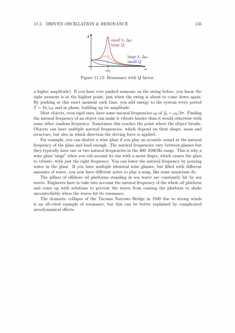
11.5. DRIVEN OSCILLATION & RESONANCE 135
ω
Asmall b, ∆ωlarge Q
large b, ∆ωsmall Q
ω0
Figure 11.12: Resonance with Q factor.
a higher amplitude). If you have ever pushed someone on the swing before, you know theright moment is at the highest point, just when the swing is about to come down again.By pushing at this exact moment each time, you add energy to the system every periodT “ 2π{ω0 and in phase, building up its amplitude.
Most objects, even rigid ones, have some natural frequencies ω0 of f0 “ ω0{2π. Findingthe natural frequency of an object can make it vibrate harder than it would otherwise withsome other random frequency. Sometimes this reaches the point where the object breaks.Objects can have multiple natural frequencies, which depend on their shape, mass andstructure, but also in which direction the driving force is applied.
For example, you can shatter a wine glass if you play an acoustic sound at the naturalfrequency of the glass and loud enough. The natural frequencies vary between glasses butthey typically have one or two natural frequencies in the 400–2500 Hz range. This is why awine glass “sings” when you rub around its rim with a moist finger, which causes the glassto vibrate, with just the right frequency. You can lower the natural frequency by pouringwater in the glass. If you have multiple identical wine glasses, but filled with differentamounts of water, you now have different notes to play a song, like some musicians do.
The pillars of offshore oil platforms standing in sea water are constantly hit by seawaves. Engineers have to take into account the natural frequency of the whole oil platformand come up with solutions to prevent the waves from causing the platform to shakeuncontrollably when the waves hit its resonance.
The dramatic collapse of the Tacoma Narrows Bridge in 1940 due to strong windsis an oft-cited example of resonance, but this can be better explained by complicatedaerodynamical effects.

136 CHAPTER 11. HARMONIC OSCILLATIONS

Chapter 12
Hydrostatics & Pressure
This part of the course will study the basics of fluid dynamics. A fluid is a substance thathas no fixed shape. They can be liquid or gas that occupy some volume and have somepressure. Ideal liquids are incompressible, while gasses are compressible; gasses tend tooccupy the volume of their container, while liquids do not. Gases are a bit more complicatedas their temperature can also vary with pressure and volume, as we will see next semesterduring the lectures on thermodynamics in PHY121. For now we will focus more on basicproperties such as pressure, density and velocity. In this chapter we will first look at thebasic concepts of hydrostatics, such as pressure.
What is pressure? Pressure P is when a total force F is applied to some surface withare A,
Pressure.P “
F
A. (12.1)
It carries units of Pascal named after Blaise Pascal (1623–1662),
1 Pa “ 1N
m2 . (12.2)
12.1 Atmospheric pressure
Otto von Guericke demonstrated the existence of atmospheric pressure in 1654 in Magde-burg. He sealed two large copper hemispheres and pumped out the air to create a vaccuuminside. Even two teams of horses could not pull apart the hemispheres, demonstrating theimmense size of the atmospheric pressure.
The atmospheric pressure at sea level is about
Patm “ 101.325 kPa “ 1013.25 hPa “ 1 atm, (12.3)
P
(a) Pressure P “ FA on a surface with area A.P
P
P
P
P
P
(b) Pressure is the same in all directions.
Figure 12.1: Pressure.
137

138 CHAPTER 12. HYDROSTATICS & PRESSURE
Table 12.1: Units of pressure. (* Per definition.)
Pa bar atm torr psi1 Pa 1 1ˆ 10´5 9.8697ˆ 10´6 7.5006ˆ 10´3 1.4504ˆ 10´4
1 hPa 1ˆ 102 “ 100* 0.001 9.8697ˆ 10´4 0.750 06 0.014 5041 kPa 1ˆ 103 “ 1000* 0.01 9.8697ˆ 10´3 7.5006 0.145 031 mbar 1ˆ 102 “ 100* 0.001 9.8697ˆ 10´4 0.750 06 0.014 5041 bar 1ˆ 105 “ 100 000* 1 0.986 97 750.06 14.50381 atm 1.013 25ˆ 104 “ 101 325* 1.0132 1 760* 14.69521 torr 133.32 1.3332ˆ 10´3 1.3160ˆ 10´3 1 0.019 3361 psi 6894.76 0.068 948 0.068 049 51.715 1
where atm is one of the alternative units for pressure, see Table 12.1. Patm is the weight(i.e. a force) of all the air above us that is spread out over some area.
How much weight does the atmosphere “feel” like on an area of A “ 1 cm2? Thetotal force would be F “ PatmA « 10.1 N, which is like having a 1 kg mass weighing onevery square centimeter. However, we do not notice this, because our bodies are internallypressurized: The pressure inside our body is the same as outside. We only experiencewhen we find ourselves in a lower-pressure environment (like on a high mountain top), orhigh-pressure one (like when diving underwater), for which our lungs and bodies were notbuilt. Deep sea fish, like the so-called “blob fish”, live at depths where the pressure is 60to 120 times higher than at sea level. At this high-pressure, they look like normal fish,but once you take them to the surface, their bodies, which have evolved for high-pressureenvironments, decompress and they become very ugly, memeable blobs.1
At any given height, a pressure pushes in all directions with the same value, as shownin Fig. 12.1b. Pressure is a scalar; it has a particular value in each point in space, but itdoes not have a particular direction. Pressure does exert a force orthogonal to a surface,but the important thing is the difference of pressure on either side of some surface. Thisis evident when you hold up the hand and feel no net force from atmospheric pressurepushing on the top, bottom, or sides. If you put your hand on the tube of a runningvacuum cleaner, there will be a pressure difference, and the your hand will be “sucked”onto the tube’s opening.
Another experiment you can try at home is holding a filled glass upside down witha coaster blocking off the opening. The coaster will stay put and block the water fromrunning out. This happens because the atmosphere applies a pressure to the coaster, evenif it is upside down. Say the beer glass has an opening of radius 4 cm, then the net forceon the coaster from the atmosphere is about Fatm « 510 N. Compare this to the weight ofthe water push down on the other side: mg « 5 N for half a liter of beer, which is abouthalf a kilogram. Clearly, the atmospheric pressure is much larger. Later in this chapter wewill see how pressure varies over height due to the added fluid weight.
12.2 Microscopic description
Why is there pressure? Where does it come from? Fluids are made out of small moleculesthat can freely move around. Each one constantly collides with others, but also with the
1In fact, something similar likely happens to an astronaut who is thrown into the vacuum of spacewithout a suit: Beside suffocating, receiving horrible radiation, having their fluids boil and bubble form intheir blood, they will swell up because all internal gas expands due to the lack of external pressure. Theirbody will not explode as in some movies, because the skin is elastic enough to withstand the increasedinternal pressure.

12.3. BULK MODULUS 139
(a) A box of colliding gasparticle has a pressure.
P
V , P , T A
(b) A container with gas closed of with apiston can measure the pressure.
Ppi = mvi
pf = mvf
(c) Gas particles collides off pistoncauses an change in momentum.
Figure 12.2: Pressure is a macroscopic phenomena caused by collisions of gas particlesbetween each other and on the wall at the microscopic level.
walls of its surrounding container. When it does, it has a change in momentum
∆p “ pf ´ pf , (12.4)
which will be normal to the wall, as in Fig. 12.2c and this causes a small force
Fi “∆pi∆t
. (12.5)
There are actually many gas molecules constantly transferring small amounts of momentumto the wall, roughly of the order of Avogadro’s number, NA Op1023q. The net force willbe experienced as a constant pressure P . We will study this in more detail as part of thetopic of statistical mechanics and thermodynamics in PHY121.
12.3 Bulk modulus
Even though we often assume solids and liquids are incompressible, in reality, they willbe somewhat compressed by a large enough pressure P . As a measure of a material’scompressibility, we define the bulk modulus
Bulk modulus.B “
´P
∆V {V, (12.6)
where the total change in volume is ∆V . The minus sign makes B positive, as ∆V ă 0.For gases the bulk modulus is very small and depends on temperature. For liquids and
solids, which are harder to compress, the bulk modulus are larger. Some examples arelisted in Table 12.2.
12.4 Pressure variation with depth
What is the pressure inside a liquid? Suppose you have a cylindrical container which isclosed at the bottom, but open at the top as in Fig. 12.3a. First consider the total force
Table 12.2: Some examples of the bulk modulus B.
Material B [Pa]Iron 100Lead 8Water 2

140 CHAPTER 12. HYDROSTATICS & PRESSURE
mg
FN
Fatm
P0 = Patm
P
A
h
(a) The force on the bottom of a container of fluidwith height h, area A is PA “ P0A` ρAhg.
h
P1P1
P2P2
P [Pa]
y [m]
y1
y2
Patm P1 P2
(b) Pressure increases linearly with depth y. The dif-ference between y1 and y2 is ∆P “ ρgpy2 ´ y1q.
Figure 12.3: The pressure in a fluid varies with depth due to weight.
on the bottom of the container. The fluid has a mass density ρ and a height h, and thecross-sectional area of the container is A, so the total weight is
Fg “ pρV qg “ ρAhg. (12.7)
At the same time, the atmosphere pushes down on the top with a pressure P0 “ Patm,
Fatm “ P0A. (12.8)
At the bottom there is a normal force holding everything in place, so at equilibrium,
FN “ Fatm ` Fg. (12.9)
Call the total pressure on the bottom P “ FN{A, then
PA “ P0A` ρAhg, (12.10)
and so the total pressure on the bottom is
Pressure variation with depth (at hydrostatic equilibrium).
P “ P0 ` ρgh. (12.11)
Note that the cross-sectional area A cancels out, so the shape of the area really does notmatter, it can be a circle, rectangle, heart, or whatever. It can even vary over the height,as the force is always “spread” out over the total area, P “ F {A.
The argumentation and result above do not only hold at the bottom of the container,but also in every point in the fluid and on the walls at any depth. So the pressure increaseslinearly with depth, but, the pressure is the same in all points as the same depth and in alldirections at equilibrium. So the pressure difference between any two depths, say y1 andy2 is
∆P “ ρgpy2 ´ y1q “ ρgh, (12.12)
if h “ y2 ´ y1 as in Fig. 12.3b.

12.5. MEASURING PRESSURE 141
Pressure Patm [hPa]
Altitudeh[km]
Everest10
20
30
40
200 400 600 800 1000
stratosphere
troposphere
1013.25 hPa
Figure 12.4: The atmospheric pressure varies with altitude. At sea-level, it is typicallyabout P “ 1013.25 hPa.
12.4.1 Air pressure variation with altitude and weather
Air pressure in reality varies by altitude. The higher you go, the less air that weighsdown on you is above you. It is more or less exponential as shown in Fig. 12.4 instead oflinear, because the density and pressure of a gas also strongly depends on the temperature.The pressure at the top of Mount Everest at 8850 m is already one third of that at sea-level, making it extremely hard to breathe for most people. The difference in pressureis noticeable when you take a sealed bag of chips up a mountain, or by the feeling onyour eardrums when you take off in an airplane (even though the cabin inside is partiallypressurized).
Local air pressure can vary wildly throughout the day from Patm “ 1013.35 hPa due toweather, with typically changes by less than 10 hPa. This is mostly caused by changes intemperature and creates so-called pressure systems that allow meteorologists to forecastthe weather. Namely, air typically flows from high to low pressure regions. Humid airfrom low-pressure regions rise up, and can condense into rain clouds, while sinking air inlow-pressure regions often brings dryer and nicer weather.
Beside variations due to weather, sea-level air pressure rises and falls up to 3 hP (closerto the equator) in 12 hour cycles due to atmospheric tides. The tides are mainly causedby thermal radiation by the sun, and to a lesser extend, the gravitational pull from themoon.
12.5 Measuring pressure
12.5.1 Manometer
A manometer is an instrument that can measure the pressure. Figure Fig. 12.5a showshow a U-shaped tube with one open end can measure the pressure P on the closed end bysimply measuring the height difference of the fluid columns. If P ą Patm, the column on
P
Patm
h
(a) A U-tube manometer can mea-sure the pressure P in the closed end.
Patm
P = 0
h
(b) A barometer measures theair pressure.
h
P = 0
Patm
(c) Torricelli’s experiment. The weightof the column creates a vacuum.
Figure 12.5: Pressure can be measured with the height of a fluid column.

142 CHAPTER 12. HYDROSTATICS & PRESSURE
the open end will be higher by a height h and vice versa if P ă Patm. If P ă Patm, thenthe pressure P on the close end must be
P “ Patm ` ρgh, (12.13)
where ρgh corresponds to the extra weight of the highest column. We measure the height,which can be expressed as
h “P ´ Patm
ρg. (12.14)
12.5.2 Barometer
A barometer measures the air pressure. The open end is again exposed to atmosphericpressure, while the closed end is completely filled with a fluid as in Fig. 12.5b. Theatmospheric pressure cannot compensate for the weight of the column if it is too high,causing the column to drop, leaving behind a vacuum where P “ 0. The air pressure thencan be measured by total height of the fluid’s column:
Patm “ ρgh. (12.15)
12.5.3 Torricelli’s experiment
This is in fact how Evangelista Torricelli (1608–1647) performed his famous experiment in1643. He filled a tube closed on one end with mercury, which is more than 13 times denserthan water, and put it upside down in a bowl as in Fig. 12.5c. This creates a vacuum onthe closed end. He used a tube of one meter, such that the mercury column height wasabout
h “Patm
ρg« 0.76 m. (12.16)
This is why the unit of pressure named after him is defined as
1 torr “1
760atm, (12.17)
where 760 mm is the nicely rounded column height. A different, but closely related unit isthe mmHg, which is almost exactly the same as one torr. This type of units are still usedin medicine as well as in weather reporting and scuba diving.
In the 4th century B.C., Aristotle postulate that “nature abhors a vacuum”, meaningthat a vacuum cannot exist stably in Nature, as surrounding matter will always fill it.With his experiment, Torricelli proved otherwise. His work led to the first speculations ofatmospheric pressure and invention of the barometer.
Table 12.3: Some examples of volumetric mass densities ρ. Some metals are indicated withatom number Z.
Material ρ [kg{m3]Gold (Z “ 79) 19 320Lead (Z “ 82) 11 340Mercury (Z “ 80) 13 534Iron (Z “ 26) 7870Cooking oil 910–930Ice 916.7Fresh water 1000Salt water 1030Wood 400–1000Air (at sea-level) 1.2

12.6. PASCAL’S PRINCIPLE 143
12.5.4 Drinking from a long straw
So what about water? The density of water is
ρ “ 1000 kg{m3 “ 1 kg{L (12.18)
by the old definition of kilogram. How long does the tube have to be to create a vacuum?Well, the minimum length is given by the condition Eq. (12.15), so about h “ 10.3 m.
When you drink cola through a straw, you create a lower pressure at the end in yourmouth by sucking. The higher atmospheric pressure then “pushes” up the cola. But ifyou have straw longer than 10.3 meters, you cannot create a pressure lower than vacuumanymore, so you will not be able to drink!
Until Torricelli’s work, people were very puzzled why their suction pumps could notpump water from wells higher than 10 meters.
12.6 Pascal’s principle
The following is very useful.
Pascal’s principle. A change in pressure in any point of an enclosed, incompress-ible fluid is transmitted undiminished to every other point in the the fluid and thewalls of the container.
This is best understood with the example of the hydraulic lift shown in Fig. 12.6. A forceF1 pushes down on the left piston with are A1. By doing so, it creates a change in pressure
∆P “F1
A1, (12.19)
which must equal the change in pressure on the piston on the right, so
∆P “F1
A1“F2
A2, (12.20)
where there is a force on the right piston,
F2 “A2
A1F1. (12.21)
This has many applications. It allows us to lift heavy things such as cars or the arm of anexcavator.
Say you want to lift a car of M “ 1500 kg from a circular hydraulic lift platform ofradius r2 “ 1 m. If the smaller circular piston has a radius r1 “ 0.1 m, then what force dowe need to hold the car in place? Using F2 “Mg and A “ πr2, we roughly find
F1 “A1
A2F2 “
r21
r22
F2 “ 150 N, (12.22)
which is the equivalent to a weight of only about 15 kg! So a 15 kg weight can compensatefor the total weight of the car, thanks to the factor of r2
1{r22.
So what if we want to lift the car by a height x2 “ 1 cm? The work to accomplish thisis
W “ F2x2, (12.23)

144 CHAPTER 12. HYDROSTATICS & PRESSURE
F1 F2
0
x1
0
x2
Figure 12.6: A hydraulic press demonstrating Pascal’s principle. A force F1 of the leftpiston with area A1 causes an force F2 “ pA2{A1qF1 on the right piston with area A2.
where F2 is the work done by the average force F2 on the large piston. The smaller pistonperforms exactly this amount of work with some average force F1, and so
F1x1 “ F2x2. (12.24)
The smaller piston has to move a distance
x1 “F2
F1x2 “
A1
A2x2 “ 1 m, (12.25)
to move the car by a one meter with a force of about 150 N!
12.7 Buoyancy
Suppose you fully submerge an object of density ρobj in a fluid with density ρ`. Everyoneknows intuitively that the object will sink if ρobj ą ρ`, and float if ρobj ă ρ`. Even if itsinks, the object will appear lighter; it will have “less weight”. The force that makes anobject float or feel lighter is called the buoyant force Fb, and it is caused by the differencein pressure with depth.
Let’s have a closer look at what exactly happens in Fig. 12.7. The fully submergedobject feels a difference in pressure between the top and bottom. The pressure on the sidescancel. The net upward force due to this pressure difference is
Fb “ F2 ´ F1 “ P2A´ P1A, (12.26)
where A is the top and bottom area of the object. From Eq. (12.12),
Fb “ pρ`ghobjqA, (12.27)
m
F2
F1mg
0
h1
h2
P
Patm
P1
P2
(a) Mass submerged at some depth. The total forcedue to pressure on the top is F1, and F2 on the bottom.
F2
+
F1
=
Fb
(b) The net upward force due to pressureis the buoyant force Fb.
Figure 12.7: A mass m that is completely submerged in a fluid at some depth experiencesa pressure differential. The pressure P2 on the bottom is larger than the pressure P1 onthe top. Pressure on the sides balance.

12.7. BUOYANCY 145
where hobj is the object’s total height. The object’s total volume is then Vobj “ Ah, so thebuoyant force for a fully submerged object is
Buoyant force (fully submerged).
Fb “ ρ`Vobjg. (12.28)
Clearly, if Fb ą mg, then the object will float to the top, while if Fb ă mg, it will sink.The mass of the object is given by m “ ρobjVobj, so the weight is given by
Wobj “ mg “ ρobjVobjg. (12.29)
Comparing to Fb “ ρ`Vobjg, we see that as expected the object floats when ρobj ă ρ` andsinks when ρobj ą ρ`.
12.7.1 Archimedes’ principle
What if the object floats and is only partially submerged as in Fig. 12.8a? The pressureon the top of the object is Patm, while on the bottom there is a pressure difference ρ`ghsub,where hsub is the height of the object that is submerged. Therefore, we can write thebuoyant force as
Fb “ ρ`V`g, (12.30)
where V` “ hsubA is the total volume of the object that is submerged. Notice that V` isactually the volume of the fluid that was displaced! This volume of the liquid has weightW` “ ρ`V`g. This is Archimedes principle:
Archimedes’ principle. Body (partially or completely) submerged in fluid is forcedup by a buoyant force equal to the weight of fluid that is displaced; Fb “ ρ`V`g.
If the body if fully submerged, h “ hsub and Vobj “ V`, and we retrieve the previousEq. (12.28). Before it is fully submerged, the buoyant force varies linearly with depth hsub,as shown in Fig. 12.8c.
hsubm
Fb
mg
(a) The object is partially sub-merged and floats if ρ ă ρ`,such that Fb ě mg.
mVobj= V`
ρ`V`
ρobjVobj
(b) At equilibrium, the weightof displaced fluid in (a) equalsthe object’s weight ρ`V`g “ mg.
Fb=ρ `Agh su
b
Fb=ρ `Agh su
b
Depth hsub
Fb
ρ`Vobjg
mg = ρobjVobjg
hobjheq
partialsubmersion
fullsubmersion
(c) Buoyant force varies with submersion hsub. Par-tially submerged, Fb “ ρ`Aghsub. Once fully sub-mersed, the buoyant force is Fb “ ρ`Vobjg.
Figure 12.8: Archimedes’ principle says that the buoyant force equals the weight of thedisplaced liquid, Fb “ ρ`V`g. If ρobj ă ρ`, the object will float, with ρ`V`g “ mg “ρobjVobjg at hydrostatic equilibrium.

146 CHAPTER 12. HYDROSTATICS & PRESSURE
At hydrostatic equilibrium, the buoyant force Fb must exactly balance the object’sweight,
Fb “ ρobjVobjg, (12.31)
or,
Condition for floating at hydrostatic equilibrium.
ρobjVobj “ ρ`V`, (12.32)
where V` is the volume of the displaced fluid, or equivalently of the part of the object thatis submerged.
12.7.2 Example: Iceberg
What fraction of a iceberg floating freely in salt water is submerged? Ice has a density ofρi “ 916.7 kg{m3, smaller than that of salt water with ρw “ 1030 kg{m3. The volume Vsub
of the iceberg that is submerged is given by Eq. (12.32):
Vsub “ρi
ρwVi, (12.33)
where Vi is the full volume of the iceberg. Therefore, the fraction that is submerged is
Vsub
Vi“
ρi
ρw“ 89%.
So the tip of the iceberg you see above sea water is only about 11% of the whole iceberg.
12.7.3 Archimedes’ trick: Measuring density
The famous legend tells the story that the king of Syracuse asked Archimedes (ca. 287–212BC) to determine if his crown was made out of pure gold without damaging it. Archimedesaccepted the challenge and started thinking. When he visited one of the public bath housesand lowered himself in the tub of water, he noticed the water level rising. This gave hima great idea to find out the density of the crown. He was so excited, he ran out into thestreets, still naked, yelling “Eureka!” (“I have found it!”). It turned out that the goldsmithhad indeed deceived the king and mixed in the cheaper and less dense silver.
Let’s study this problem. Say you have a mass m that is denser than water, ρobj ą ρ`.You submerge it fully in a container with water and hold it in the middle with a wire like inFig. 12.9. Without the water, the wire would have a tension T “ mg equal to the weight,but now there is the additional buoyant force making the mass appear lighter:
T “ mg ´ Fb. (12.34)
m
FbT
mg
Figure 12.9: Object with higher mass density than the fluid, ρ ą ρ` is held in place by awire.
12.7. BUOYANCY 147
With a scale we can measure the weight Wobj “ mg and the new apparent weight T . Sincethe object is fully submerged, Fb “ ρ`Vobjg, which is the weight
W` “ m`g “ ρ`V`g (12.35)
of the total volume of displaced fluid, V` “ Vobj, with mass m` “ ρ`V`. Therefore, we canwrite the object’s density relative to water as
ρobj
ρ`“m{Vobj
m`{V`. (12.36)
The volumes cancel and we can substitute the weights
ρobj
ρ`“
m
m`“mg
W`. (12.37)
By Archimedes’ principle, Fb “W`, such that
ρobj
ρ`“
mg
mg ´ T. (12.38)
There are two ways to find the density ratio: Either you weigh the displaced water to findm`, or you measure the tension T . The displaced water can be weighed by pouring off thewater above the normal level and placing it on a scale, or if you know the container’s areaand ρ` simply by measuring difference of the water level. The tension can be measuredwith a Newton meter, like a spring scale, or an old-fashioned balance scale.

148 CHAPTER 12. HYDROSTATICS & PRESSURE

Chapter 13
Fluids in motion
13.1 Continuity equation
Suppose you have a pipe as in Fig. 13.1a that has two sections with different cross-sectionalareas A1 and A2. Water flows through the pipe, and now suppose some section of water ofvolume V1 enters the first section with some velocity v1. The volume can be expressed as
V1 “ A1v1∆t, (13.1)
where `1 “ v1∆t is the distance traveled in time interval ∆t. By the same argument, thevolume in the second section is
V2 “ A2v2∆t. (13.2)
We assume that the fluid is incompressible, such that for the same ∆t, V1 “ V2, and
A1v1∆t “ A2v2∆t, (13.3)
or,
A1v1 “ A2v2 “ const. (13.4)
We define the volume flow rate, or current flow,
Current flow.Iv “ Av, (13.5)
which has units m3{s. We now arrive at a special equation that deserves its own box:
Continuity equation.Iv “ Av “ const. (13.6)
This equation simply tells us that the flow that goes in a pipe on what end, must comeout on the other. So if the area A gets bigger, then the velocity gets bigger, then velocitydecreases.
149

150 CHAPTER 13. FLUIDS IN MOTION
A1
A2
v1 v2
`1
`2
(a) Pipe with two segments of cross-sectional areaA1 and A2.
P1
P2
v1
v2F2
`1`2
A1
A2
h1
h2F1
(b) Pipe with two segments of volumes V1 and V2 andcross-sectional area A1 and A2 at different heights.
Figure 13.1: Fluids in pipes with different shapes and cross-sectional areas.
13.2 Bernouilli’s equation
What if the pipe changes height in a gravitational field as in Fig. 13.1b? If the fluid israised by some height h, it will lose some kinetic energy and gain potential energy, andvice versa if the fluid is lowered by some height. In some ∆t, some small volume ∆V of thefluid with mass ∆m “ ρ∆V gets lifted by a height h “ h2 ´ h1. The change in potentialenergy for such a volume is
∆U “ ∆mgh “ ρ∆V gh, (13.7)
which can be negative or positive depending on the sign of h “ h2´h1. The correspondingchange in kinetic energy is,
∆K “1
2∆mv2
2 ´1
2∆mv2
1 (13.8)
The work-energy theorem states that the total work done by the fluid is
W “ ∆U `∆K, (13.9)
or,
W “ ρ∆V gh`1
2ρ∆V pv2
2 ´ v21q. (13.10)
But we know that work comes from force times distance, W “ F∆x, so where does theforce come from? In the case of these fluids, there has to some pressure that pushes thefluid through the pipe. The force at the bottom of the pipe, F1, comes from some pressureP1, and the opposing force F2 at the top of the pipe comes from pressure P2. At thebottom, we have
W1 “ F1∆x1 “ P1A1∆x1 “ P1∆V , (13.11)
while at the top for ∆V “ A2∆x2,
W2 “ ´P2∆V , (13.12)
where the minus sign indicates that F2 is opposite to ∆x2 and F1. Then, the total workdone is
W “W1 `W2 “ pP1 ´ P2q∆V . (13.13)
We compare this equation to Eq. (13.13), and find
P1 ´ P2 “ ρgh`1
2ρpv2
2 ´ v21q (13.14)
Reshuffling, we arrive at Bernoulli’s equation:
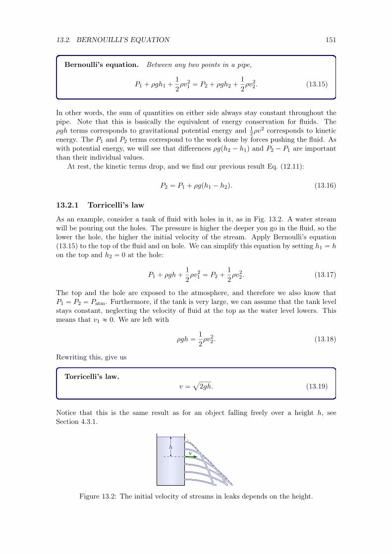
13.2. BERNOUILLI’S EQUATION 151
Bernoulli’s equation. Between any two points in a pipe,
P1 ` ρgh1 `1
2ρv2
1 “ P2 ` ρgh2 `1
2ρv2
2. (13.15)
In other words, the sum of quantities on either side always stay constant throughout thepipe. Note that this is basically the equivalent of energy conservation for fluids. Theρgh terms corresponds to gravitational potential energy and 1
2ρv2 corresponds to kinetic
energy. The P1 and P2 terms correspond to the work done by forces pushing the fluid. Aswith potential energy, we will see that differences ρgph2 ´ h1q and P2 ´ P1 are importantthan their individual values.
At rest, the kinetic terms drop, and we find our previous result Eq. (12.11):
P2 “ P1 ` ρgph1 ´ h2q. (13.16)
13.2.1 Torricelli’s law
As an example, consider a tank of fluid with holes in it, as in Fig. 13.2. A water streamwill be pouring out the holes. The pressure is higher the deeper you go in the fluid, so thelower the hole, the higher the initial velocity of the stream. Apply Bernoulli’s equation(13.15) to the top of the fluid and on hole. We can simplify this equation by setting h1 “ hon the top and h2 “ 0 at the hole:
P1 ` ρgh`1
2ρv2
1 “ P2 `1
2ρv2
2. (13.17)
The top and the hole are exposed to the atmosphere, and therefore we also know thatP1 “ P2 “ Patm. Furthermore, if the tank is very large, we can assume that the tank levelstays constant, neglecting the velocity of fluid at the top as the water level lowers. Thismeans that v1 « 0. We are left with
ρgh “1
2ρv2
2. (13.18)
Rewriting this, give us
Torricelli’s law.v “
a
2gh. (13.19)
Notice that this is the same result as for an object falling freely over a height h, seeSection 4.3.1.
hv
Figure 13.2: The initial velocity of streams in leaks depends on the height.

152 CHAPTER 13. FLUIDS IN MOTION
A1 A2
v1 v1v2v2
P1
P2
Figure 13.3: Pipe with two segments of cross-sectional area A1 and A2.
13.2.2 Venturi effect
Now consider a fluid moving trough a pipe with a cross-sectional area A1 that has a narrowmiddle section with area A2 ă A1 as in Fig. 13.3. We assume that the pressure P1 is thesame on either end, and that the height does not change. We are therefore left with thecontinuity equation,
v2 “A1
A2v2. (13.20)
If A2 is more narrow, A2 ă A1, then the velocity has to be larger there, v2 ą v1. What isthe pressure there? Bernouilli’s equation reduces to
P1 `1
2ρv2
1 “ P2 `1
2ρv2
2. (13.21)
Since v2 ą v1, the pressure will drop in the narrow section, P2 ă P1. This is called theVenturi effect.
Venturi effect. The pressure of a fluid decreases when its speed increases.
When large vehicles, like trucks or trains, move by very fast, it can feel as if they aresucking you in due to the pressure drop. Similarly, when a train enters a narrow tunnelat high speed, the air between the train and tunnel walls suddenly speed up, and you cansometimes feel the difference in pressure on your ear drums.
An experiment that you can try at home is the following. Hold a piece of paper by thecorners of a short end close to your mouth, and blow above it. Because the fast air passingabove, the paper will lifted upward. This is similar to how some airplane wings can createa lift: Due to its shape, the air above the wing will travel faster than the air below.
13.3 Current resistance & viscous flow
Bernouilli’s equation states pressure is the same anywhere in a pipe at constant height andconstant area. However, in practice, we see that there is a pressure drop ∆P across thepipe. This can be explained by a drag force on the fluid coming from the pipe’s surface andfrom each the fluid itself. To see why the fluid exerts a drag force on itself, imagine differentconcentric layers of the fluid as in Fig. 13.4a. The outer layer is dragged by the surface, andgets slowed down. This layer in turn, slows down the next layer due to internal friction,etc. Typically, the fluid will move faster in the center than close to the pipe’s surface.There is a pressure difference that is proportional to the current flow,
Pressure drop due to drag.
∆P “ P1 ´ P2 “ RIv, (13.22)

13.4. LAMINAR & TURBULENT FLOW 153
with Iv “ vA again, and where R is a constant of resistance. The larger R, the larger thedrag, and the larger the pressure drop. The resistance for steady flow in a pipe is
Resistance for steady flow in a cylindrical pipe.
R “8ηL
πr4, (13.23)
where L and r are the length and radius of the pipe, respectively, and η is the coefficientof viscosity that depends on the material. A high viscosity means a large drag (like honeyor crude oil), while low viscosity means the fluid can easily flow with too much drag (likewater).
To define the viscosity η, take two plates that each have an area A and are separatedby a height z. Suppose there is a fluid in between, that we imagine has different layers as inFig. 13.4b. We push the top plate with some force F , such that it has a constant horizontalvelocity v. The fluid below will also start to move due to drag, but the drag is larger closerto either plates. We see that the velocity continuously varies with z. Experimentally, it isfound that
F “ηvA
z. (13.24)
By measuring the speed v for a given force F , we obtain η. Notice that the units of η areN s{m2 or Pa s. It even has its own units of Poise (P),
1 P “ 0.1 Pa. (13.25)
From Eqs. 13.22 and 13.23 we see that the flow for a cylindrical pipe is
Iv “ ∆P
ˆ
πr4
8ηL
˙
. (13.26)
There are several interesting conclusions one can draw from this equation. For the samepressure difference ∆P , the flow rate depends on r4. For the same pressure difference ∆Pand radius r, the flow rate is inverse proportional to the pipe’s length L.
13.4 Laminar & turbulent flow
A flow that can be thought of as moving in separate, adjacent layers that do not mix asin Fig. 13.4a, is called laminar.
Consider you put an obstacle in a fluid that is in laminar flow. For small velocities, thefluid will smoothly flow around the object without mixing its layers, such that after passing
(a) Pipe with laminar flow: Layer close to the wall go slowerdue to drag forces.
Fv
Az
0
h
(b) Defining the viscosity η by movingthe the top plate.
Figure 13.4: In laminar flow, you can cleanly divide up the moving fluids into layers movingwith their own speed.

154 CHAPTER 13. FLUIDS IN MOTION
(a) Laminar flow with an obstacle. Thelayers do not mix.
(b) Under some conditions, an objectcauses turbulence after.
Figure 13.5: An obstacle in a flow of fluid can cause turbulence.
the obstacles, it will still continue as laminar flow. This is shown in Fig. 13.5a. (Note thatthe velocity of flow is relative: The fluid can move, while the object is stationary, but theobject can also be moving in a stationary fluid.)
At large velocities, however, there will be a transition from laminar to turbulent flow,depicted in Fig. 13.5b. Here the layers of the fluids start mixing and the moving in a chaotic,unpredictable pattern. This happens at some critical velocity, which can be understoodwith Reynold’s number,
Reynold’s number in a cylindrical pipe.
NR “2rρv
η. (13.27)
The Reynold’s number does not have any units. It gives the condition of type of flow. IfNR ă 2000, then the flow will be laminar. If NR ą 3000, then the flow will be turbulent.Between 2000 and 3000 there will be some transition regime. So if a laminar fluid startsmoving very fast, it will become more turbulent.
If the pressure difference ∆P across a pipe is higher, the velocity v and Reynold’snumber NR will become larger and the flow will become turbulent. The turbulence willreduce the overall flow as shown in Fig. 13.6.
13.5 Magnus effect
A object that is rotating and moving relative to a fluid will experience a net force. This iscalled the Magnus effect and is depicted in Fig. 13.7.
Remember the Venturi effect: If the fluid’s velocity increases, then the pressure de-creases. Because the object is rotating, the relative velocity between the object’s surfaceand the fluid will be larger on one side than the other. This generates a pressure difference,and therefore a net force that tends to push the object from the high pressure toward thelow pressure.
Pressure difference ∆P
Flo
w
laminar turbulent
Figure 13.6: Flow becomes turbulent at large pressure differences ∆P . At higher ∆P , thevelocity v and Reynold’s number NR will become larger.

13.5. MAGNUS EFFECT 155
v
FMaglow
pressure
highpressure
Figure 13.7: A rotating object moving relative to a fluid will feel a difference in pressure,causing a net force FMag.
The Magnus effect allows players in baseball and football to curve a ball by giving itthe right spin when throwing or kicking it. Similarly, a golf ball with backspin will spinhigher into the air than with the same velocity but no spin.

156 CHAPTER 13. FLUIDS IN MOTION

Chapter 14
Surface tension
As we have seen in the last few chapters, a random point inside a fluid feels pressure fromall sides due to molecules constantly colliding into each other and their container. However,the molecules of the fluid can in addition be attracted to each other due to cohesive forces.A random molecule inside a liquid will feel an equal attractive force from all directions,causing them to cancel. A molecule that is on the surface of the liquid, however, will onlyfeel a cohesive force from this liquid below and from the sides, shown in Fig. 14.1a. Theforces from the liquid molecules underneath are therefore unbalanced, and causes a pullinward. This generates some internal pressure that will deform the surface to minimizethe area. The so-called surface tension is the total unbalanced force from the molecules ofliquid below. The liquid’s surface, as a consequence, acts as a stretchable membrane thatcan carry the weight of a light object that would otherwise sink (ρobj ą ρ`), like a needleor insect.
If you look more closely at the cross section of a floating needle on a water surface, youwould see that the surface, otherwise flat, is indented as in Fig. 14.1b. Over the whole areawhere the needle is touching the water, there is a force Fst which is balancing the forceof gravity Fg “ mg. In general, the surface tension Fst on a thin object like a needle, isproportional to the total length L of the object,
Surface tension on a thin, long object.
Fst “ γL, (14.1)
where γ is a constant that depends on the liquid and its temperature. It is defined as the
(a) The attractive force on a molecule inside theliquid cancel, but not on the surface. The surfacewill act as a stretchable membrane.
mg
Fst,1Fst,2 θ θ
mg
Fst,1Fst,2 θ θ
(b) The total surface tension Fst from the points of contactbalances the weight of the needle, Fg “ mg. The weakerthe surface tension, the deeper the indent.
Figure 14.1: The surface tension of a liquid can balance a metal needle with ρobj ą ρ`.
157

158 CHAPTER 14. SURFACE TENSION
θCθC
(a) Convex meniscus with θC ą 90˝ hasstronger cohesion than adhesion.
θCθC
(b) Concave meniscus with θC ă 90˝ hasstronger adhesion than cohesion.
Figure 14.2: Capillary action
amount of force per unit length,
γ “Fst
2L. (14.2)
The needle indents the surface, and there is a surface tension form either side, as shown inFig. 14.1b. Therefore, the vertical component of the total surface tension is
Fst,y “ Fst,1 cos θ ` Fst,2 cos θ “ pγLq cos θ. (14.3)
The needle floats as long as Fst,y ą mg, and the surface will change shape to find equilib-rium.
The angle θ decreases for larger needle’s mass m. The maximum mass mmax of a needlewith length L that the surface tension can carry is when θ “ 0, such that
mmax “2γL
g. (14.4)
14.1 Surfactants & soap bubbles
Soap, whose molecule has one hydrophilic end that attracts water, can lower the surfacetension of water, causing an insect of needle to sink through. Soap is therefore called asurfactant (from “surface-active agent”).
Surfactants in combination with water can create foam and bubbles. Without a surfac-tant, the water surface tension is too large to form stable bubbles. Soapy water will createa film, which is a thin layer of water that is between two layer of soap. Soap moleculeshave one greasy, hydrophobic end that stick out to the outside of the film and protectsthe water from evaporation, prolonging the bubble’s lifetime. When a soap film enclosessome air, it will form a sphere to minimize the surface tension, and therefore the area. Thepressure of the trapped air is slightly increased to balance the internal pressure due to thesurface tension.
14.2 Capillary action
One consequence of surface tension is capillary action. This comes from the attractiveadhesive forces between the liquid and walls of the container. If the adhesive forces withthe wall are larger than the cohesive forces between the molecules, the surface will makea “U” shape (i.e. concave). If the cohesive forces are larger than the adhesive forces, thesurface will curve upward in the middle (i.e. convex ). A curved surface of a liquid is calleda meniscus. This can be described by the contact angle between the surface and the wall,θC, shown in Fig. 14.2.
The contact angle θC depends on the fluid and container materials. For water in a glasscontainer, θC “ 0, creating a very concave-shaped meniscus. For mercury with glass, it isθC “ 140˝, creating a concave meniscus.