A Rapid Prototyping Tool for Embedded, Real-Time Hierarchical Control Systems

Hindawi Publishing CorporationEURASIP Journal on Embedded SystemsVolume 2008, Article ID 162747, 14 pagesdoi:10.1155/2008/162747

Research ArticleA Rapid Prototyping Tool for Embedded, Real-TimeHierarchical Control Systems

RamRajagopal,1 Subramanian Ramamoorthy,2 Lothar Wenzel,3 and Hugo Andrade3

1 Electrical Engineering and Computer Sciences, University of California at Berkeley, Berkeley, CA 94720-1770, USA2School of Informatics, The University of Edinburgh, Edinburgh, EH9 3JZ, UK3National Instruments Corp., Austin, TX 78759, USA

Correspondence should be addressed to Ram Rajagopal, [email protected]

Received 24 May 2007; Revised 25 February 2008; Accepted 17 May 2008

Recommended by Shuvra Bhattacharyya

Laboratory Virtual Instrumentation and Engineering Workbench (LabVIEW) is a graphical programming tool based on thedataflow language G. Recently, runtime support for a hard real-time environment has become available for LabVIEW, whichmakes it an option for embedded systems prototyping. Due to its characteristics, the environment presents itself as an idealtool for both the design and implementation of embedded software. In this paper, we study the design and implementation ofembedded software by using G as the specification language and the LabVIEW RT real-time platform. One of the main advantagesof this approach is that the environment leads itself to a very smooth transition from design to implementation, allowing forpowerful cosimulation strategies (e.g., hardware in the loop, runtime modeling). We characterize the semantics and formal modelof computation of G. We compare it to other models of computation and develop design rules and algorithms to propose soundembedded design in the language. We investigate the specification and mapping of hierarchical control systems in LabVIEW andG. Finally, we describe the development of a state-of-the-art embedded motion control system using LabVIEW as the specification,simulation and implementation tool, using the proposed design principles. The solution is state-of-the-art in terms of flexibilityand control performance.

Copyright © 2008 Ram Rajagopal et al. This is an open access article distributed under the Creative Commons Attribution License,which permits unrestricted use, distribution, and reproduction in any medium, provided the original work is properly cited.

1. INTRODUCTION

LabVIEW (Laboratory Virtual Instrumentation and Engi-neering Workbench) is a graphical programming environ-ment, developed by National Instruments Corp., based onthe dataflow paradigm. It was originally targeted towards thetest, measurement, and automation industries.

In recent years there has been tremendous growth in theembedded software and systems market. It is driven by theneed for low cost, fast and portable solutions with short timeto market. National Instruments Corp. developed LabVIEWReal Time (LabVIEW RT) to cater to these demands. TheLabVIEW RT environment includes the original LabVIEWenvironment, as well as an ETS/vxWorks-based real-timehardware system that includes modules for data acquisitionand control.

In the LabVIEW environment, programs are describedusing the G programming language. Broadly, this languagecan be understood as a structured dataflow programming

language. The environment integrates a compiler and sched-uler for the G language. In LabVIEW RT, these compilerand scheduler have been extended to generate executableprograms from G that can be executed in real-time operatingsystems, such as RTOS. Using the current compiler andscheduler, the complete language specification can be exe-cuted in the system, but only with soft real-time constraints.

The objective of this paper is to outline a framework forusing the LabVIEW RT software and hardware environmentsfor embedded systems design in a principled way, avoidingissues that compromise real-time operation performance.Whenever required, we consider specifically LabVIEW RTversion 7.1. We summarize our contributions.

In Section 2, we provide a formal description of the Glanguage. We determine some important characteristics ofthe language. We compare the G model of computation toother comparable models in the literature.

In Section 3, we show how programs can be specifiedin G in order to satisfy some important requirements

2 EURASIP Journal on Embedded Systems

for programs that define embedded systems. We developprinciples so that G programs compiled and scheduled byLabVIEW RT are sound according to the stated require-ments. We also compare the LabVIEW RT environment andsome other tools available for embedded systems design anddeployment.

In Section 4, we show how a complete solution for anembedded control system can be developed and deployedusing the proposed environment. Our chosen application isembedded motion control, a general task that is a corner-stone of many manufacturing automation applications. It isalso a staple hierarchical control system. The algorithms usedto implement the solution use the principles developed inprevious sections. We propose some novel approaches whichare enabled by the environment, among them an onlinedesign based on qualitative control definition. The design isperformed online, as the system is operating.

In Section 5, we discuss the changes in standard controldesign practice that become possible by using LabVIEW RTand G. Such changes should also be available to any designtool that implements the toolset currently available in theproposed language and system. In Section 5, we concludeand propose future works.

2. THE G LANGUAGE

In this section, we explore the specification and properties ofthe G programming language. We also compare the languageto other dataflow specification languages in the literature.

2.1. Specification of G

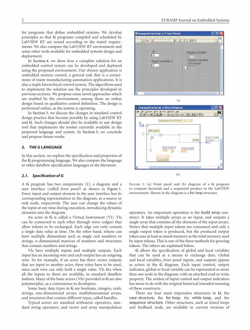
A G program has two components [1]: a diagram and auser interface (called front panel) as shown in Figure 1.Every input and output element in the user interface has itscorresponding representation in the diagram, as a source orsink node, respectively. The user can change the values ofthe input at any time during execution, introducing dynamicelements into the diagram.

An actor in G is called a Virtual Instrument (VI). VIscan be connected to each other through wires (edges) thatallow tokens to be exchanged. Each edge can only containa single data value at time. On the other hand, tokens canhave multiple dimensions such as single real numbers orstrings, n-dimensional matrices of numbers and structuresthat contain numbers and strings.

VIs have multiple inputs and multiple outputs. Eachinput has an incoming wire and each output has an outgoingwire. So for example, if an actor has three vector outputsthat are input to another actor, three wires have to be used,since each wire can only hold a single value. VIs fire whenall the inputs to them are available, in standard dataflowfashion. Many of the basic actors (VIs) provided in G are alsopolymorphic, as a convenience to developers.

Some basic data types in G are booleans, integers, reals,strings, one-dimensional arrays, multidimensional arrays,and structures that contain different types, called bundles.

Typical actors are standard arithmetic operators, stan-dard string operators, and vector and array manipulation

0Input variable 2

0N Display double

0

0 0

Output variable(1D array)

(a)

Computing vector of k! for k = 1, · · · ,n

Shift register

NNI32

1

+1

×

i

Input variable 2 Display double

×

Display double

DBLDBL

Local variable

Tunnel[I32]

Output variable(1D array)

(b)

Figure 1: (a) Front panel and (b) diagram of a G programto compute factorials and a sequential product in the LabVIEWenvironment. Shown in the diagram is a for loop structure.

operators. An important operation is the build array con-struct. It takes multiple arrays as an input, and outputs asingle array that contains all the elements of the input arrays.Notice that multiple input tokens are consumed and only asingle output token is produced, but the produced outputtoken uses at least as much memory as the total memory usedby input tokens. This is one of the three methods for growingtokens. The others are explained below.

G allows the specification of global and local variablesthat can be used as a means to exchange data. Globaland local variables, front panel inputs, and outputs appearas actors in the G diagram. Each input control, outputindicator, global or local variable can be represented as morethan one node in the diagram, with an attached read or writeproperty. The notion of input control and output indicatorshas more to do with the original historical intended meaningof these constructs.

There are four main imperative structures in G: thecase structure, the for loop, the while loop, and thesequence structure. Other structures, such as timed loopsand feedback node, are available in current versions of

Ram Rajagopal et al. 3

LabVIEW RT. We do not address them here, but theirsemantics satisfy the properties discussed in the paper.

All structures are integrated into the general program-ming paradigm by working as a capsule that contains all theactors inside it. The structure executes when all inputs tothe actors inside it become available. Tokens enter and exitthe structures through tunnels. Graphically, the structureis appropriately represented as an object that envelops theselected actors (Figure 1(b)).

The for loop is a standard loop where at each iteration allthe VIs inside it are fired as data to their inputs and outputsbecome available. The next iteration is only executed afterall VIs in the loop have fired. The number of iterations isspecified as an input to the loop actor.

In the situation in Figure 1(b), for example, the productbetween variable Display Double and Input Variable2 is computed and stored in Display Double througha local variable. In parallel, the current loop index i ismultiplied by the last factorial variable calculation stored ina shift register. The output is put back in the shift register.Both of these parallel operations are only executed againwhen the loop executes again.

The for loop includes two loop specific features: theshift register and a tunnel. The shift register is a con-struct that stores the token input to it (right-hand side inFigure 1(b)) and makes it available at the next iteration (left-hand side in Figure 1(b)). It is a memory. A shift registercan be extended to remember any number of values,but this number is fixed prior to the compilation of theprogram. The output tunnel construct is also a form oflocal memory. It can be configured to either remember thelast value input into it, or more interestingly to grow amultidimensional token by appending incoming tokens. Inthe example discussed, the output token from the tunnelwill be an array of integers of size N . The behavior of thetunnel can be reproduced by using a shift register fed withthe output of a build array, which has as inputs the outputof the shift register and the token connected to the tunnel.

The while loop is similar to the for loop except that aconditional statement inside the loop determines when theloop stops executing. The conditional statement can be aboolean output of an actor built out of comparison functionsavailable in G.

The sequence structure is a structure comprised of mul-tiple frames. Actors inside each frame can receive inputs fromoutside the structure, as well as from VIs in previous frames.The sequence structure enforces an ordered execution of theactors firing, having priority over the token driven firing.

Finally, the case structure is a structure comprised ofmultiple frames with a selector input. According to the tokenthat arrived in the selector input, only one frame is executed.The only caveat for the case structure is that all frameshave to produce the same outputs to the remaining programoutside the structure. This means that the frame selection canonly change the value of the token, but not their type nor thenumber of tokens outputted.

Feedback loops are not allowed in G, so no actor can bepart of a feedback loop without a delay. Even if the output of

a local variable is connected to the input of a local variable,the data firing rule imposes an implicit ordering.

2.2. Properties of G

A comprehensive characterization of G is presented in [2]using formal terminology of dataflow languages [3]. In thissection, we summarize and expand on that. G can be char-acterized as a homogeneous, dynamic, multidimensionalstructured dataflow based language.

G can be categorized as a structured dataflow languagesince the semantics are expressed using a combination ofconstructs from imperative and functional languages.

G is homogeneous because every actor consumes orproduces a single token for a given edge in the graph. Thetoken can be a complex structure whose size can changeduring execution, as long as the dimensionality remainsconstant.

G is multidimensional since tokens can have multipledimensions and dynamic since there are constructs that allowpart of the program graph to be conditionally executed basedon data.

The complete model of G cannot be statically sched-uled because it has several structures and actors whosebehavior depends on input data. Examples of this includecase structures and loops controlled by inputs from the userinterface.

G is Turing complete [2, 4] and local/global variablesallow nondeterminism [5] to arise. One example of non-determinism is shown in Figure 1(b), where the valueof Display Double depends on Input Variable 2. Ifthe value of Input Variable 2 is changed in the userinterface while the loop executes, the output value ofDisplay Double will depend on whether the change wasread in the current or the next iteration. This point iselaborated in Section 3.

A very important property is that G is always compos-able. Several VIs in a diagram can be gathered into a singleone, as long as there are no feedback loops, without affectingthe behavior of the program. This can be done because thegraph is homogeneous and delay-less feedback loops arenot allowed. Another consequence is that every G graph isdirected and has a multiple source, multiple sink structure.

2.3. G and othermodels of computation

Although G does not fit exactly into any of the presentedmodels, it shares characteristics with several of them asdescribed below.

(i) Process Networks (PN): By definition a ProcessNetwork (PN) is a very generic model of computation, whereconcurrent processes communicate through unidirectionalFIFO channels [6]. In G, processes (actors) can also com-municate through global and local variables. These variablesare not FIFO and cannot write an infinite amount of data oninputs/outputs [2]. Therefore, the complete G model cannotbe classified as a PN. But G keeps some resemblance to PN, asevery VI is a small process that generates tokens of arbitrarysize with fixed dimension.


(ii) Integer Dataflow (IDF): The homogeneous IDFmodel [7] is a model that resembles G by restricting the useof global and local variables. The main differences are that inG tokens can be multidimensional and flow control is donethrough case structures and while loops. A complete G graphcan be quasi-statically scheduled [2].

(iii) Synchronous Dataflow (SDF): A restricted versionof G, in which switch actors, case structures, while loops,global and local variables, and data dependent for loopsare not allowed, can be modeled as a homogeneous SDF[8] and thus statically scheduled. Multidimensional SDF(MSDF) [9] is an extension to SDF, where actors produceand consume n-dimensional rectangles of data. G cannot bewell characterized by MSDF because any array data exchangein G is done through a single multidimensional token.Also another important difference is that every actor in Gconsumes (produces) a single token from each of its inputs(outputs).

(iv) Finite State Machines (FSM): G can be used toexpress Finite State Machines [10]. A standard FSM templatecan be easily constructed for G (e.g., [1]). Note that itis possible to integrate the FSM concept into a dataflowframework. Local and global variables could be used to sharedata between such state machine and a normal dataflowprogram.

3. EMBEDDED DESIGN IN LabVIEW ANDG

There are many different definitions for embedded software.A popularly accepted definition is that it is a software systemwith extremely restricted user interface that acts on infinitestreams of data. The desired requirements for specifying andexecuting an embedded program can be listed as follows [5].

(i) Requirement 1. The program specification shouldpreferably be determinate, and therefore the outputs shouldbe consistent with the inputs, regardless of execution details.Also the program specification should be sample rateconsistent and causal. In a sample rate consistent program,actors consume and produce tokens in a balanced way, thatis, we can find integer firing rates such that the dataflow canbe executed repeatedly. In a causal specification, outputs ofeach actor depend only on current and past inputs.

(ii) Requirement 2. The scheduler should implementa complete execution of the program so that a non-terminating program does not deadlock.

(iii) Requirement 3. The scheduler should execute abounded program in bounded memory. A bounded programis a program where the number of tokens at every edge isbounded by some finite constant in a complete execution ofthe program. In the G context, since each edge can only haveone token, but tokens can grow in size, a bounded programis a program whose memory requirements are bounded.

These requirements ensure that a well-behaved programoperates properly in embedded environments. Notice thatRequirement 1 refers directly to the specification language,whereas Requirements 2 and 3 refer to how the compilationenvironment and the scheduler are able to handle thespecification language. In some situations, the specification

language is such that the scheduler requirements are enforceddirectly by constraints in the language itself. For example,in homogeneous synchronous dataflow systems, there is nopossibility of deadlocks.

In this section we will present algorithms and program-ming guidelines that guarantee that the main requirementsare met, thus allowing LabVIEW RT and G to be trans-parently used in embedded software design, while loosingminimal expression power. We then proceed to compareLabVIEW-RT and G with other standard popular embeddedprogramming languages.

We assume that the standard compiler and scheduler inLabVIEW-RT is used. In order to derive our algorithms andrestrictions, we will also assume that for every execution ofthe G program the front panel input values are fixed. Intypical industrial situations, the values are indeed fixed, andthe program is autonomously run such as in the motioncontrol example in this section.

3.1. Determinism and consistency

A G graph is always sample rate consistent because itis homogeneous. Also causality is guaranteed because thesemantics do not allow for delay-less feedback loops.

Due to the semantics, non-determinism only arises in Gwhen local or global (storage) variables are used as part ofa diagram. Due to the fact that G allows multiple reads andwrites to local and global variables, race conditions may arise.For example, a simple program where two instantiations ofa single local variable are connected to different constants isnondeterministic.

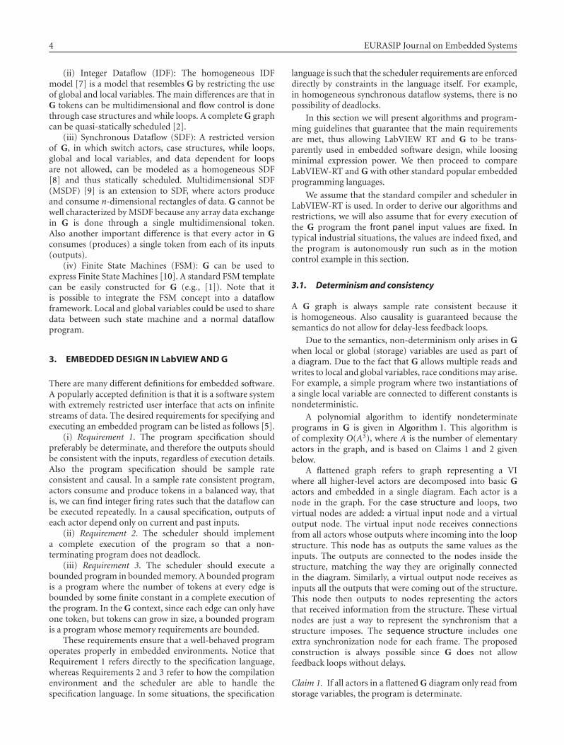
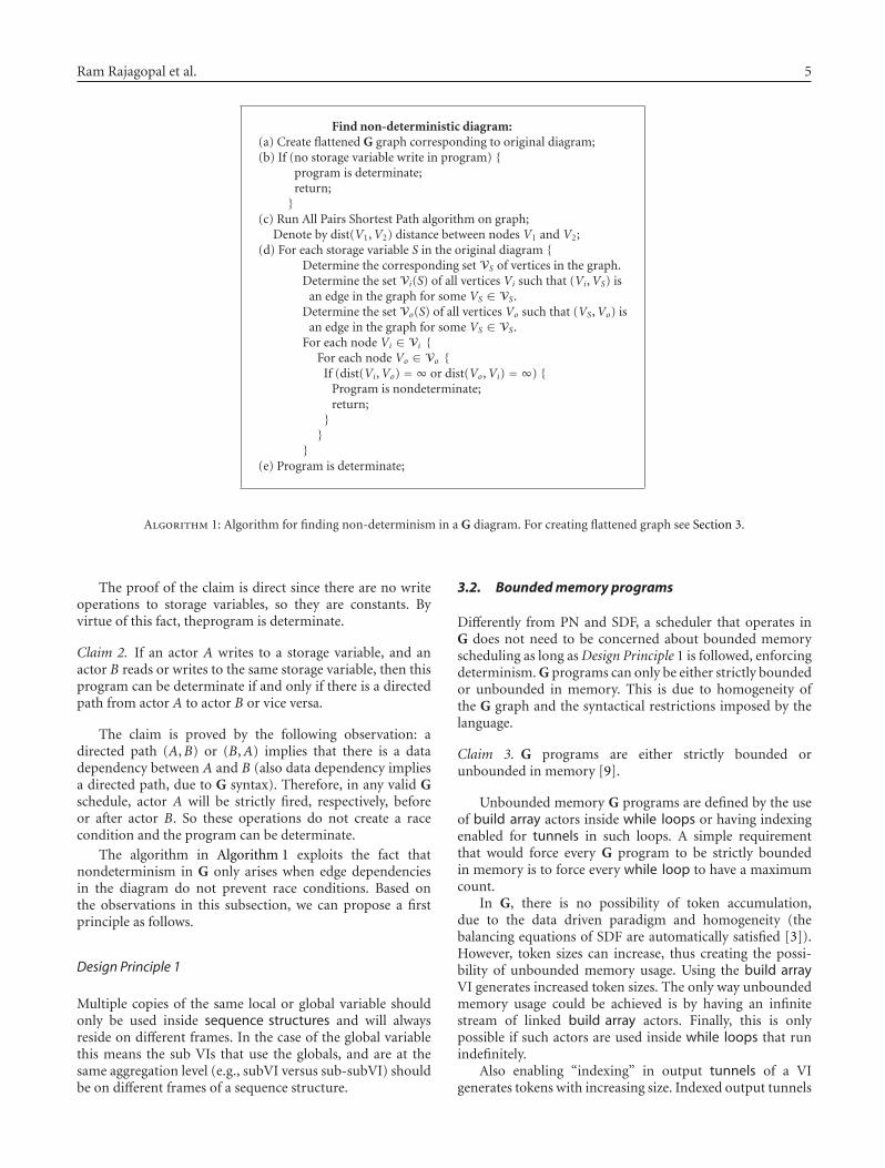
A polynomial algorithm to identify nondeterminateprograms in G is given in Algorithm 1. This algorithm isof complexity O(A3), where A is the number of elementaryactors in the graph, and is based on Claims 1 and 2 givenbelow.

A flattened graph refers to graph representing a VIwhere all higher-level actors are decomposed into basic Gactors and embedded in a single diagram. Each actor is anode in the graph. For the case structure and loops, twovirtual nodes are added: a virtual input node and a virtualoutput node. The virtual input node receives connectionsfrom all actors whose outputs where incoming into the loopstructure. This node has as outputs the same values as theinputs. The outputs are connected to the nodes inside thestructure, matching the way they are originally connectedin the diagram. Similarly, a virtual output node receives asinputs all the outputs that were coming out of the structure.This node then outputs to nodes representing the actorsthat received information from the structure. These virtualnodes are just a way to represent the synchronism that astructure imposes. The sequence structure includes oneextra synchronization node for each frame. The proposedconstruction is always possible since G does not allowfeedback loops without delays.

Claim 1. If all actors in a flattened G diagram only read fromstorage variables, the program is determinate.


Find non-deterministic diagram:(a) Create flattened G graph corresponding to original diagram;(b) If (no storage variable write in program) {

program is determinate;return;}

(c) Run All Pairs Shortest Path algorithm on graph;Denote by dist(V1,V2) distance between nodes V1 and V2;

(d) For each storage variable S in the original diagram {Determine the corresponding set VS of vertices in the graph.Determine the set Vi(S) of all vertices Vi such that (Vi,VS) is

an edge in the graph for some VS ∈ VS.Determine the set Vo(S) of all vertices Vo such that (VS,Vo) is

an edge in the graph for some VS ∈ VS.For each node Vi ∈ Vi {

For each node Vo ∈ Vo {If (dist(Vi,Vo) = ∞ or dist(Vo,Vi) = ∞) {

Program is nondeterminate;return;}}

}(e) Program is determinate;

Algorithm 1: Algorithm for finding non-determinism in a G diagram. For creating flattened graph see Section 3.

The proof of the claim is direct since there are no writeoperations to storage variables, so they are constants. Byvirtue of this fact, theprogram is determinate.

Claim 2. If an actor A writes to a storage variable, and anactor B reads or writes to the same storage variable, then thisprogram can be determinate if and only if there is a directedpath from actor A to actor B or vice versa.

The claim is proved by the following observation: adirected path (A,B) or (B,A) implies that there is a datadependency between A and B (also data dependency impliesa directed path, due to G syntax). Therefore, in any valid Gschedule, actor A will be strictly fired, respectively, beforeor after actor B. So these operations do not create a racecondition and the program can be determinate.

The algorithm in Algorithm 1 exploits the fact thatnondeterminism in G only arises when edge dependenciesin the diagram do not prevent race conditions. Based onthe observations in this subsection, we can propose a firstprinciple as follows.

Design Principle 1

Multiple copies of the same local or global variable shouldonly be used inside sequence structures and will alwaysreside on different frames. In the case of the global variablethis means the sub VIs that use the globals, and are at thesame aggregation level (e.g., subVI versus sub-subVI) shouldbe on different frames of a sequence structure.

3.2. Boundedmemory programs

Differently from PN and SDF, a scheduler that operates inG does not need to be concerned about bounded memoryscheduling as long as Design Principle 1 is followed, enforcingdeterminism.G programs can only be either strictly boundedor unbounded in memory. This is due to homogeneity ofthe G graph and the syntactical restrictions imposed by thelanguage.

Claim 3. G programs are either strictly bounded orunbounded in memory [9].

Unbounded memory G programs are defined by the useof build array actors inside while loops or having indexingenabled for tunnels in such loops. A simple requirementthat would force every G program to be strictly boundedin memory is to force every while loop to have a maximumcount.

In G, there is no possibility of token accumulation,due to the data driven paradigm and homogeneity (thebalancing equations of SDF are automatically satisfied [3]).However, token sizes can increase, thus creating the possi-bility of unbounded memory usage. Using the build arrayVI generates increased token sizes. The only way unboundedmemory usage could be achieved is by having an infinitestream of linked build array actors. Finally, this is onlypossible if such actors are used inside while loops that runindefinitely.

Also enabling “indexing” in output tunnels of a VIgenerates tokens with increasing size. Indexed output tunnels


are just a graphical representation for a build array combinedwith a shift register structure.

Real-time performance degrades in programs wherememory usage is increasing or unpredictable, making itattractive to keep G programs bounded in memory. We canstate the following.

Design Principle 2

While loops should always have a maximum iteration con-dition. Furthermore, for efficiency, whenever possible, arraysshould be preinitialized using initialize array and filled upusing replace array subset actors, avoiding the memoryuncertainties of the build array actor.

3.3. Complete execution

Based on the semantics of G, and because it is homogeneous,it is clear that any valid schedule guarantees completeexecution of a determinate program. There will be nodeadlocks unless they are induced by actor behavior (e.g.,infinite while loop). Notice that Requirement 2 is again arequirement in the scheduler in LabVIEW, but that due to thestructure of G, using Design Principle 1 and Design Principle2 we are able to guarantee sound behavior for the systemindependently of scheduling decisions. Thus we have thefollowing.

Claim 4. Given a determinate G diagram, there is alwaysa valid schedule that consists of a sequential Breadth FirstSearch [11] order firing of every actor on the diagram.This implies that the G diagram can never deadlock. Anyscheduler for G will be able to satisfy Requirement 2.

Claim 4 states that every determinate diagram has a validexecution schedule that satisfies Requirement 3. In fact, if themaximum count requirement is satisfied, then no G programwill ever deadlock due to program specification.

To prove the claim true, using the composability princi-ple, we can construct a diagram where every structure (whileloops, for loops, case and sequence structures) is inside aseparate SubVI. We also add a virtual source that is connectedto every other source in the graph. In this diagram the validschedule consists of firing all actors in a breadth first search(BFS) order, starting at the virtual source. The BFS searchorder guarantees that all actors (including switches) will beappropriately fired, as all inputs to every actor will alreadybe available when it is its turn to be executed. The subVIsthat include case structures can also be fired on the BFSorder, except that a specific path will be chosen dependingon the control input. But still a path should exist due to Gsyntax restrictions. The diagram of composed subVIs thatcontain while loops or for loops can be looped and firedrepeatedly. In fact if we are dealing with a G program withmaximum loop counts, then all loops can be replaced by theirdecomposed versions. Now we have the original situationagain and thus the BFS search can be applied.

3.4. LabVIEW-RT/G and other tools

In many applications it may be required that a certainperiodic schedule be executed within a hard-timed loop.For example, in a digital control application hard timing isextremely important to ensure system stability [12].

LabVIEW-RT was developed to allow a hard timedexecution of a G diagram. It consists of an execution kernel(RT Engine) that runs the G diagram on the RTOS real-time operating system. The execution kernel is supported bya standard industrial PC (based on a PXI chassis) equippedwith a National Instruments data acquisition board. In thiswork, development was done on a host desktop computerusing a LabVIEW-RT interface. The host computer is linkedto the RT embedded controller system, to download theprogram and update the user interface.

We can compare LabVIEW and G to some popularembedded system development languages and tools. Wefocus on hybrid languages [13], since they seem to be themost adopted in current real-time system development.

One feature of LabVIEW and G is that the real-timeruntime environment, and the simulation environment usethe same compiler and scheduler, which facilitates embeddedcontrol systems development, since usually in this domainextensive simulations are performed, including hardware inthe loop tests, before a first prototype.

(i) Esterel [14] is a hybrid language that combinesconstructs of imperative languages with some facilities ofdata flow languages, such as concurrency and preemption.The language has a synchronous model of time. Signals canbe present or absent, and in each clock cycle the programawakens reads inputs and produces outputs. The languageis determinate in that signal checks are always performedbefore block execution. Compared to Esterel, LabVIEW andG offer two main differences: signals are always presentand programs are represented as diagrams. Furthermore,causality violations are easily avoided in G if proposed designprinciples are followed.

(ii) SDL is a graphical language defined by the ITU [15].A program consists of concurrent FSMs, each with a singleinput queue and communication channels to communicateamong them. Execution might be nondeterministic since theorder of arrival of tokens to the different queues dependson execution speed of each FSM. An SDL program canbe emulated in G using the concurrency available in thelanguage, but this sacrifices determinism. A better approachis to design a sequenced parallel FSM implementation usingthe sequence structure. The main advantages of LabVIEWand G are imperative constructs, efficient compilation, andease of implementation of dataflows, which are crucial incontrol and signal processing applications.

(iii) SystemC is a C++ based language for systemmodeling, that implements a discrete-event computationmodel. The language provides libraries that specify pro-cessing modules and specify input-output ports for com-munication. The language is both a description languageand a simulation kernel, making it easier to transitionfrom specification to executable implementation. LabVIEWoffers some important advantages compared to System


Table 1: Hybrid language features compared. Full support •, and partial support ◦. Part of the table in [13]. CCSS refers to CoCentric SystemStudio, imp. to implementation and mgmt. to management. ∗Support in LabVIEW through timed loops.

Features Esterel SDL SystemC CCSS G

Concurrent • • • • •Hierarchy • • • • •Preemption • • • •Deterministic • ◦ • •Synchronous commn. • • • •Buffered commn. • • • •FIFO commn. • ◦ • •Procedural • ◦ • ◦ ◦Finite-State-Machines • • ◦ • •Dataflow • • • •Multi-rate dataflow ◦ • •∗Software imp. • • • • •Hardware imp. • • • •Memory mgmt. ◦ • •

C: automated and efficient memory management, whichprevent memory leaks, and a dataflow-based environment.

(iv) CoCentric System Studio [16] is a hierarchicalspecification language that combines PNs, FSMs, and gatedmodels. Dataflow block primitives can be written in C++.The development environment offers a simple simulationand debugging mode, as well as support for code generation.Compared to CoCentric modeling, the main advantage ofLabVIEW is that the simulation and execution platformsare the same, and automated memory management. Signalprocessing and control libraries are available to both.

(v) Simulink is a system level description environment[17], based on the computational algebra tool Matlab.Simulink has a real-time code generation module Real-TimeWorkshop, that allows described systems to be downloadedto specific real-time boards. Interactivity and online exper-imentation are very complicated in this environment sinceeach time a real-time program is to be run, it needs to berecompiled. The user interfaces are also not easy to create andmodify as compared to LabVIEW.

(vi) Some other languages that are used, but are muchless popular, are PMC and Forth [18]. PMC is based ona mathematical abstraction called process algebra. It doesnot support object orientation nor dynamic allocation ofmemory, but has primitives for synchronization. Forth is animperative interpreted language, which supports a variety ofprocessors.

4. EMBEDDEDMOTION CONTROL

Modern motion systems, such as robots, involve a variety ofdifferent elements that come together in a complex system.On the one hand, they are constructed from electrome-chanical components that combine mechanical elementssuch as wheels and gearboxes with electrical componentssuch as power converters, digital circuits, and solid-statesensors. The operation of these electromechanical systems

is choreographed by embedded software programs thatabstract the dynamics of these interacting elements andprovide a basis for higher level programs that performreasoning and deliberation. For instance, the mechanicalcomponents are subject to physical constraints, the electricalcomponents involve a variety of transient dynamics and thecommunication channels between low-level elements involvesignificant uncertainty. The role of the low-level embeddedsoftware programs is to hide this complexity and providesimpler symbolic or logical variables with which to deliberateat the higher level.

These notions of hierarchy and modularity represent oneof the best ways to overcome system-level complexity, in avariety of different domains [19]. However, the way thesenotions have been brought to bear on typical motion systemshas involved difficult tradeoffs.

In many robots, including some fairly modern examplessuch as Sony’s AIBO and its many clones, the joint-level control modules handle all of the above mentionedcomplexity and expose a limited set of parameters to thehigher level programs. So, even though the joints areequipped with servo motors and sophisticated circuity thatcould—in principle—support many different model-basedand adaptive control strategies, what the user actually getsis a PID controller with limited control over setpoint, risetime, and such variables. This has the important implicationthat task-level control algorithms are now restricted toonly dealing with kinematic variables and not with thetrue dynamics of the robot. Moreover, this approach leadsto algorithmic limitations at the higher level (e.g., in theexpressiveness of the planning and control strategy) that havelittle to do with the task at hand and much more to dowith architectural decisions regarding the embedded systemimplementation.

In response to these limitations, there is growing interestin developing tools and techniques that can span the entirespace from high-level specification (such as “go from A


Desiredtrajectory

Analyze/storeHost (PC)

Shared memory interface

Motion board

RT trajectorySplining

PID control

Mechanical device

(a)

Qualitativeoptimal design

Trajectory Learnsystem

Host program

PC

Senddata

Command

HomeControlSysid

Getdata

Embedded controllerReal plant

Simulatedplant

RT(PXI)

(b)

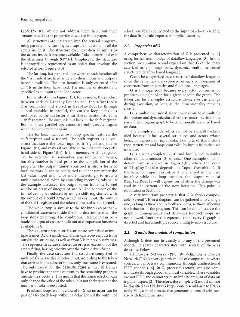
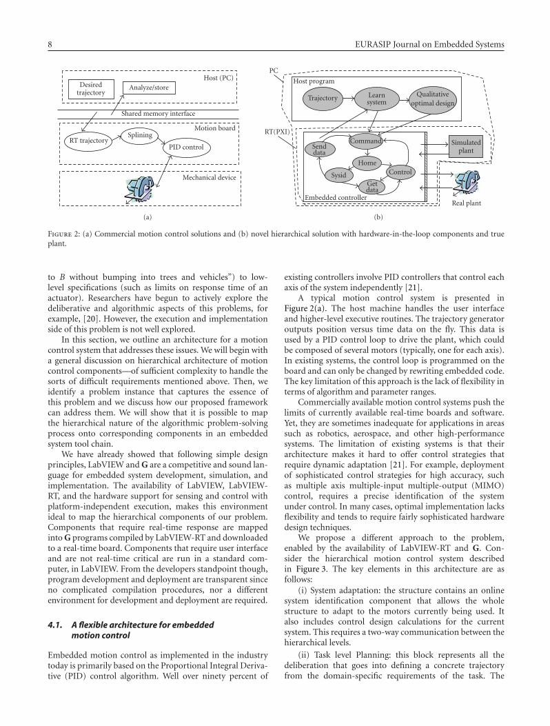
Figure 2: (a) Commercial motion control solutions and (b) novel hierarchical solution with hardware-in-the-loop components and trueplant.

to B without bumping into trees and vehicles”) to low-level specifications (such as limits on response time of anactuator). Researchers have begun to actively explore thedeliberative and algorithmic aspects of this problems, forexample, [20]. However, the execution and implementationside of this problem is not well explored.

In this section, we outline an architecture for a motioncontrol system that addresses these issues. We will begin witha general discussion on hierarchical architecture of motioncontrol components—of sufficient complexity to handle thesorts of difficult requirements mentioned above. Then, weidentify a problem instance that captures the essence ofthis problem and we discuss how our proposed frameworkcan address them. We will show that it is possible to mapthe hierarchical nature of the algorithmic problem-solvingprocess onto corresponding components in an embeddedsystem tool chain.

We have already showed that following simple designprinciples, LabVIEW and G are a competitive and sound lan-guage for embedded system development, simulation, andimplementation. The availability of LabVIEW, LabVIEW-RT, and the hardware support for sensing and control withplatform-independent execution, makes this environmentideal to map the hierarchical components of our problem.Components that require real-time response are mappedinto G programs compiled by LabVIEW-RT and downloadedto a real-time board. Components that require user interfaceand are not real-time critical are run in a standard com-puter, in LabVIEW. From the developers standpoint though,program development and deployment are transparent sinceno complicated compilation procedures, nor a differentenvironment for development and deployment are required.

4.1. A flexible architecture for embeddedmotion control

Embedded motion control as implemented in the industrytoday is primarily based on the Proportional Integral Deriva-tive (PID) control algorithm. Well over ninety percent of

existing controllers involve PID controllers that control eachaxis of the system independently [21].

A typical motion control system is presented inFigure 2(a). The host machine handles the user interfaceand higher-level executive routines. The trajectory generatoroutputs position versus time data on the fly. This data isused by a PID control loop to drive the plant, which couldbe composed of several motors (typically, one for each axis).In existing systems, the control loop is programmed on theboard and can only be changed by rewriting embedded code.The key limitation of this approach is the lack of flexibility interms of algorithm and parameter ranges.

Commercially available motion control systems push thelimits of currently available real-time boards and software.Yet, they are sometimes inadequate for applications in areassuch as robotics, aerospace, and other high-performancesystems. The limitation of existing systems is that theirarchitecture makes it hard to offer control strategies thatrequire dynamic adaptation [21]. For example, deploymentof sophisticated control strategies for high accuracy, suchas multiple axis multiple-input multiple-output (MIMO)control, requires a precise identification of the systemunder control. In many cases, optimal implementation lacksflexibility and tends to require fairly sophisticated hardwaredesign techniques.

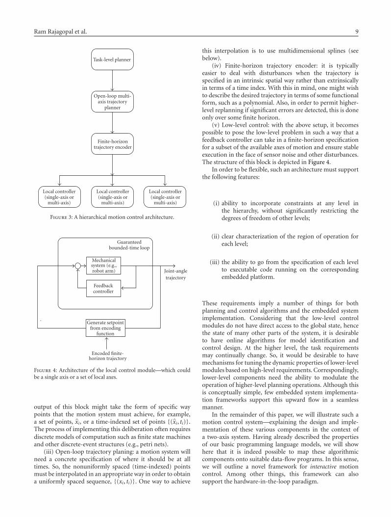
We propose a different approach to the problem,enabled by the availability of LabVIEW-RT and G. Con-sider the hierarchical motion control system describedin Figure 3. The key elements in this architecture are asfollows:

(i) System adaptation: the structure contains an onlinesystem identification component that allows the wholestructure to adapt to the motors currently being used. Italso includes control design calculations for the currentsystem. This requires a two-way communication between thehierarchical levels.

(ii) Task level Planning: this block represents all thedeliberation that goes into defining a concrete trajectoryfrom the domain-specific requirements of the task. The


Task-level planner

Open-loop multi-axis trajectory

planner

Finite-horizontrajectory encoder

Local controller(single-axis or

multi-axis)


multi-axis)


multi-axis)

Figure 3: A hierarchical motion control architecture.

Guaranteedbounded-time loop

Mechanicalsystem (e.g.,robot arm)

Feedbackcontroller

Generate setpointfrom encoding

function

Joint-angletrajectory

Encoded finite-horizon trajectory

Figure 4: Architecture of the local control module—which couldbe a single axis or a set of local axes.

output of this block might take the form of specific waypoints that the motion system must achieve, for example,a set of points, xi, or a time-indexed set of points {(xi, ti)}.The process of implementing this deliberation often requiresdiscrete models of computation such as finite state machinesand other discrete-event structures (e.g., petri nets).

(iii) Open-loop trajectory planing: a motion system willneed a concrete specification of where it should be at alltimes. So, the nonuniformly spaced (time-indexed) pointsmust be interpolated in an appropriate way in order to obtaina uniformly spaced sequence, {(xi, ti)}. One way to achieve

this interpolation is to use multidimensional splines (seebelow).

(iv) Finite-horizon trajectory encoder: it is typicallyeasier to deal with disturbances when the trajectory isspecified in an intrinsic spatial way rather than extrinsicallyin terms of a time index. With this in mind, one might wishto describe the desired trajectory in terms of some functionalform, such as a polynomial. Also, in order to permit higher-level replanning if significant errors are detected, this is doneonly over some finite horizon.

(v) Low-level control: with the above setup, it becomespossible to pose the low-level problem in such a way that afeedback controller can take in a finite-horizon specificationfor a subset of the available axes of motion and ensure stableexecution in the face of sensor noise and other disturbances.The structure of this block is depicted in Figure 4.

In order to be flexible, such an architecture must supportthe following features:

(i) ability to incorporate constraints at any level inthe hierarchy, without significantly restricting thedegrees of freedom of other levels;

(ii) clear characterization of the region of operation foreach level;

(iii) the ability to go from the specification of each levelto executable code running on the correspondingembedded platform.

These requirements imply a number of things for bothplanning and control algorithms and the embedded systemimplementation. Considering that the low-level controlmodules do not have direct access to the global state, hencethe state of many other parts of the system, it is desirableto have online algorithms for model identification andcontrol design. At the higher level, the task requirementsmay continually change. So, it would be desirable to havemechanisms for tuning the dynamic properties of lower-levelmodules based on high-level requirements. Correspondingly,lower-level components need the ability to modulate theoperation of higher-level planning operations. Although thisis conceptually simple, few embedded system implementa-tion frameworks support this upward flow in a seamlessmanner.

In the remainder of this paper, we will illustrate such amotion control system—explaining the design and imple-mentation of these various components in the context ofa two-axis system. Having already described the propertiesof our basic programming language models, we will showhere that it is indeed possible to map these algorithmiccomponents onto suitable data-flow programs. In this sense,we will outline a novel framework for interactive motioncontrol. Among other things, this framework can alsosupport the hardware-in-the-loop paradigm.


4.2. Online implementation of system identificationand control components

4.2.1. System identification

Model-based control design begins with the definition andidentification of a suitable model of the dynamics of thesystem. Often, there is insufficient information available toderive these models form first principles. Instead, the pre-ferred approach is to observe the behavior of the system, interms of input-output data, and infer the underlying modelthrough the algorithmic process of system identification. ForDC motors, the system model in Laplace s-domain

P(s) = Km

s2 + Tms(1)

captures the physical behavior appropriately, where theparameters can be physically interpreted as a signal gain,Km, and time constant, Tm. The parameters can be identifiedfollowing a procedure that minimizes the error between theobserved output y and the estimated output y for a giveninput x [22, 23]:

J∗ = minTm ,Km

N∑

k=1

[

y(k)− y(k)]2. (2)

The model derived for a single axis can be naturallygeneralized to multiple axes. For most usual systems, axistransfer functions can be identified independently.

The optimization in (2) can only be solved if the systembeing identified is stable. In our approach, we use a simplestabilizing controller for each axis. For the single axis, asimple proportional gain controller can always stabilize it,albeit inefficiently. The plant can be identified using thiscontroller. Mathematical details can be derived followingtechniques in [12].

4.2.2. Control design

A controller architecture that satisfies our requirements offlexibility and interactivity is the linear quadratic regulator(LQR). This controller can be used for a single-axis or fora local channel of multiple axes, and is compatible with thescheme depicted in Figure 4. In this section, we will brieflydescribe this controller and we will specifically point outhow this structure supports interlevel communication: (a)in allowing a higher-level module to adjust the dynamicproperties and (b) in indicating that the system has exitedits region of applicability and higher-level replanning isnecessary. We build our multiple axis system model from theidentified parameters using a linear state space system model

x(t) = Ax(t) + Bu(t), (3)

where x(t) ∈ Rn and u(t) ∈ Rm are the state and controlactions , respectively. The control task, that of executing agiven finite-horizon trajectory segment, can be defined bya cost function that specifies costs on deviation from thisdesired trajectory,

J = x′(T)QTx(T) +∫ T

0

(

x′(t)Qx(t) + u′(t)Ru(t))

dt, (4)

where QT , Q and R are symmetric positive definite matricesrepresenting costs. A higher level module is free to set thesematrices separately for each trajectory segment—and in thissense, the problem is flexible. Using optimal control [12],the above problem can be solved by using an input u(t) =−R−1B′K(t)x(t), where x(t) is the observed state. The gainfunction K(t) is calculated solving a nontrivial optimizationproblem, and depends on the choice of the matrices Q, QT ,and R.

In particular, the gain matrices can be parameterizedin simple ways such that intuitive concepts such as stiff ofsmooth response may be mapped onto them. For instance,consider the matrix form Q = diag(a1, a1, a2, a2) where alloff-diagonal elements are zero. The parameters a1, a2 cannow control the relative importance of trajectory followingand minimum effort. This is appealing to a typical user ofindustrial motion systems.

The LQR controller represents an “automatic” designprocedure that is only valid within a specific region ofapplicability, which can be computed using sophisticatedapproximation methods [24]. So, for instance, if we knowthe maximum energy that can be applied by an actuator,then we can restrict the region of operation and the lowestlevel module is now in a position to influence a higher-levelplanning module by indicating an exit from the safe region.This is a desirable aspect of the flexible architecture.

4.3. Integration of design components

In this section, we map the proposed hierarchical systemmodel and online algorithms to an actual embedded systemfor generic motion control. When compared with existingmotion control architectures, the LabVIEW RT-based systemprovides an easy way to use, flexible control environment.

Our system encapsulates a mechanism for the user tostart with unknown plant parameters, identify the parame-ters experimentally, design a control algorithm, and run iton real-time hardware in one seamless system. Furthermore,control design can be executed in real time with effectsof varying cost choices observed immediately in systemresponse. This level of design integration is new in embeddedmotion control.

The software-hardware mapping of the new architectureis shown in Figure 2(b). Compare this to existing commercialarchitectures shown in Figure 2(a). The host program runsin a desktop PC. The real-time embedded controller runs ina commercial PXI computer system, with LabVIEW RT andRTOS installed. The embedded controller and host programare completely implemented in G. The host computer andthe PXI system communicate via a TCP/IP-based protocol.This enables the RT subsystem to be used anywhere in adistributed system and still be controlled by the host.

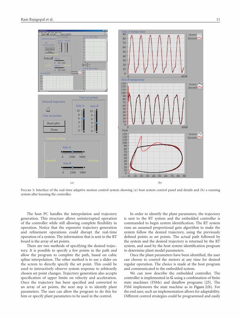
We start by describing the host software. A straightfor-ward user interface has been implemented for the system(Figures 5(a) and 5(b)). It allows the user to start with aqualitative plant model (in fact can be more general thanthe DC motor), identity unknown plant parameters, designand implement a control strategy. Furthermore, a high-leveldesired trajectory can be specified for a designed system.


User set points

Axis B10

86420

Axis A10

7

3

0

Desired trajectory

User set points

Reset plot

DoneControl setting

Leahn off

AccurateSmooth Axis B

0 500 1000

Axis A

0 500 1000

0123456789Axis B versus time

01

23

45

67

8

9Axis A versus time

4

6

810

1214Desired path

DesiredExecuted

Axis A

1086420

Axis B

108642

0

User set pointsDesired trajectory

User set points

Reset plot

Done

Control setting

Axis A

0 2500 5000AccurateSmooth

Axis B

0 2500 5000

(a)

0 10 20 30 40 50 60 70 80 900

102030405060708090

100110120130Path

Desired

Executed

0 49400

102030405060708090

100110120130Axis B versus time

Desired

Executed

0 49390

1020

3040

50

60

7080

90Axis A versus time

Desired

Executed

(b)

Figure 5: Interface of the real-time adaptive motion control system showing (a) host system control panel and details and (b) a runningsystem after learning the controller.

The host PC handles the interpolation and trajectorygeneration. This structure allows uninterrupted operationof the controller while still allowing complete flexibility inoperation. Notice that the expensive trajectory generationand refinement operations could disrupt the real-timeoperation of a system. The information that is sent to the RTboard is the array of set points.

There are two methods of specifying the desired trajec-tory. It is possible to specify a few points in the path andallow the program to complete the path, based on cubicspline interpolation. The other method is to use a slider onthe screen to directly specify the set point. This could beused to interactively observe system response to arbitrarilychosen set point changes. Trajectory generation also acceptsspecification of upper limits on velocity and acceleration.Once the trajectory has been specified and converted toan array of set points, the next step is to identify plantparameters. The user can allow the program to do this forhim or specify plant parameters to be used in the control.

In order to identify the plant parameters, the trajectoryis sent to the RT system and the embedded controller iscommanded to begin system identification. The RT systemruns an assumed proportional gain algorithm to make thesystem follow the desired trajectory, using the previouslydefined points as set points. The actual path followed bythe system and the desired trajectory is returned by the RTsystem, and used by the host system identification programto determine plant model parameters.

Once the plant parameters have been identified, the usercan choose to control the motors at any time for desiredregular operation. The choice is made at the host programand communicated to the embedded system.

We can now describe the embedded controller. Thecontroller is implemented in G using a combination of finitestate machines (FSMs) and dataflow programs [25]. TheFSM implements the state machine as in Figure 2(b). Forthe end user, such an implementation allows for adaptability.Different control strategies could be programmed and easily


added as a new state in the controller. The communi-cation and input/output infrastructure would remain thesame.

Currently, the FSM in the controller can be directed torun either a simple gain algorithm for system identificationor a MIMO feedback algorithm, with gains chosen by theinteractive control design program in the host PC. Thechoice is dictated by a command from the host program.The FSM responds to requests that arrive via a TCP/IPqueue from the host program. The FSM architecture allowsmultiple control algorithms to be stored in the embeddedcontrollers allowing any one to be immediately invoked whencommanded.

In our hierarchical approach, the desktop PC handlesall user interface-oriented functions and the embeddedcontroller handles the stringent real-time control loop. Thetwo processes are capable of communicating with each other.However, the absence of the communication link does notaffect the operation of the control loop. This brings anelement of fault tolerance to the system.

A major feature of the proposed interface and systemis that the user can dynamically modify control parametersand experiment with the plant response. This allows multiplecontrol strategies to be compared in a “what-if” simulationor even in real-time execution. The host program alsoimplements a simulation of the estimated plant, so thatthe system response can be simulated before being sent tomotor control. When the user changes to control parameterseem satisfactory in simulation, this data can be immediatelyrelayed to the embedded controller.

We have implemented an intuitive slider-based controldesign. The slider ranges from smooth to accurate. Insmooth mode, the control response is slower, but there areno overshoots when following trajectories. In the accuratemode, response is faster, and depending on the choice,overshoot can happen. The interesting feature here is that theresponse of the whole system is fast enough that moving theslider, one can immediately see the effects on a real system, ifthis is desired.

Another important characteristic of the system is thatthe structure allows the real plant to be replaced by asimulated plant in software without requiring significantmodifications. This technique (called “Hardware in theloop” abbreviated HIL) [26] is a popular system verificationand simulation tool. Traditional systems do not have sucha well-defined and easy-to-use interface to support HILexperiments, especially for user-defined algorithms.

Currently a two-axis controller running at frequencies upto 10 KHz is supported by the system. It is expected that suchhigh frequencies are attainable even with more sophisticatedcontrol structures and algorithms.

5. EMBEDDED CONTROL DESIGN USING LabVIEW RT

Some important requirements for successful developmentenvironment for embedded programs in control are as fol-lows:

(i) facilitate development of reliable programs;

(ii) simplify integration of different levels of a hierarchy,making it easy to map into different platforms (e.g.,real time, FPGA);

(iii) availability of standard control design and signalprocessing routines;

(iv) source code needs to be easy to maintain;

(v) code should be easy to read and interpret;

(vi) parallelism and concurrency are easy to represent.

The proposed system description language and designenvironment address all these issues as shown in earliersections, as long as simple design principles are followed.

Previous works in COSSAP [27], GRAPE [28], Simulink[17], and Ptolemy [29] have shown the importance ofusing higher-level representation constructs to build real-time functionality. The applications there have focused onmultirate signal processing, with online adaptation andlearning for a variety of tasks such as channel equalizationand echo cancelation [30]. The transparent transition froma simulation environment to a real deployment has beenstudied for such problems.

Control programs on the other hand are typicallyhierarchical as explained in Section 4. The motion controlapplication developed in this paper demonstrates two novelpossibilities: the mapping of hierarchical control structuresinto an embedded execution platform, and the handling ofa variety of different problem time scales in a transparentmanner. The later capability in fact shows an interestingnew direction for control systems design, where even morecomplicated design optimizations are done in real time,based on observation of current system performance, ina typical hierarchical feedback loop. The design of theG language and the integration level of the LabVIEW-RTenvironment were helpful to achieve these goals.

5.1. Design process

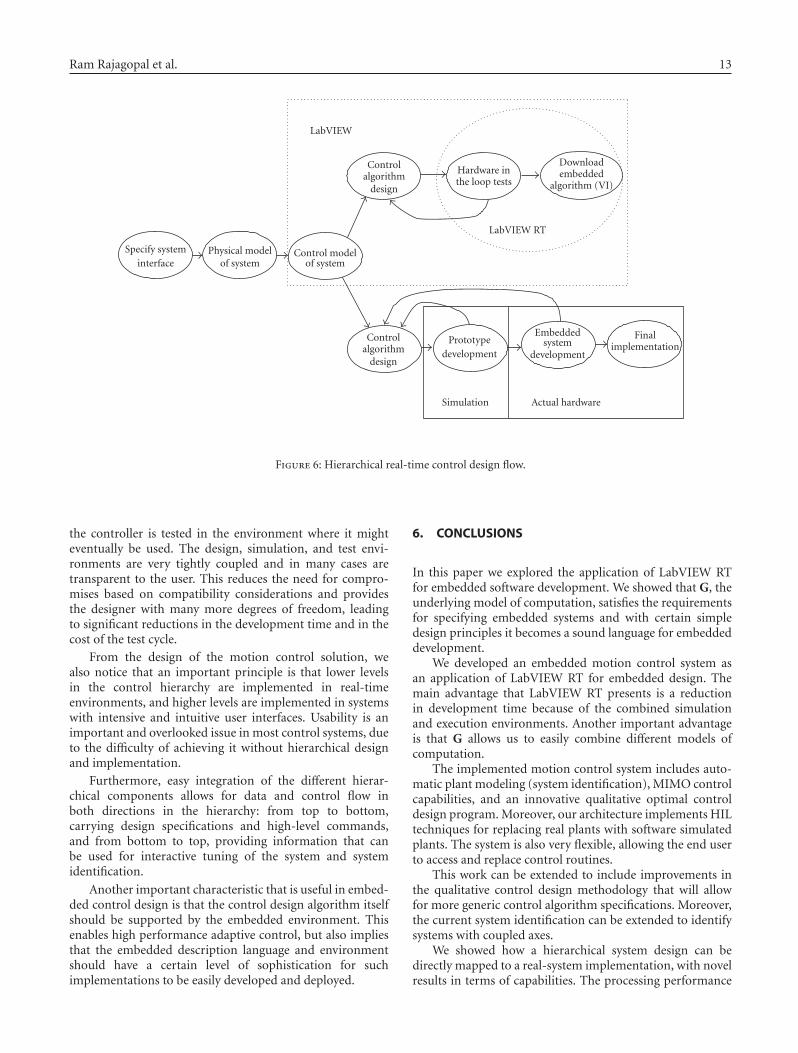
In Figure 6, we compare the traditional design process withthe new design process that becomes possible as a result ofour system architecture. We show this comparison in termsof the example application developed in this paper.

In the traditional design process a model of the systemis used to devise a possible control strategy. This is testedwith a computer-based simulation and then ported to aprototype hardware test rig. This process is iterative and eachiteration leads closer to the final product. The key issue hereis that the design, simulation, testing, and integration aredone using an array of loosely coupled tools. There are notightly integrated system design environments that allow thedesigner to simulate and test the design iteratively withouthaving to move between multiple programs, maybe evenmultiple platforms. Recent advances in hardware softwarecodesign address the problem of optimum design of asubsystem. They do not address the larger issue of integratingdissimilar subsystems in a time and cost optimal manner.

A design generated in the LabVIEW RT environmentis directly used for hardware-in-the-loop simulations where


Downloadembedded

algorithm (VI)

Hardware inthe loop tests

Controlalgorithm

design

Control modelof system

Physical modelof system

Specify systeminterface

LabVIEW RT

LabVIEW

Controlalgorithm

design

Prototypedevelopment

Simulation

Embeddedsystem

development

Actual hardware

Finalimplementation

Figure 6: Hierarchical real-time control design flow.

the controller is tested in the environment where it mighteventually be used. The design, simulation, and test envi-ronments are very tightly coupled and in many cases aretransparent to the user. This reduces the need for compro-mises based on compatibility considerations and providesthe designer with many more degrees of freedom, leadingto significant reductions in the development time and in thecost of the test cycle.

From the design of the motion control solution, wealso notice that an important principle is that lower levelsin the control hierarchy are implemented in real-timeenvironments, and higher levels are implemented in systemswith intensive and intuitive user interfaces. Usability is animportant and overlooked issue in most control systems, dueto the difficulty of achieving it without hierarchical designand implementation.

Furthermore, easy integration of the different hierar-chical components allows for data and control flow inboth directions in the hierarchy: from top to bottom,carrying design specifications and high-level commands,and from bottom to top, providing information that canbe used for interactive tuning of the system and systemidentification.

Another important characteristic that is useful in embed-ded control design is that the control design algorithm itselfshould be supported by the embedded environment. Thisenables high performance adaptive control, but also impliesthat the embedded description language and environmentshould have a certain level of sophistication for suchimplementations to be easily developed and deployed.

6. CONCLUSIONS

In this paper we explored the application of LabVIEW RTfor embedded software development. We showed that G, theunderlying model of computation, satisfies the requirementsfor specifying embedded systems and with certain simpledesign principles it becomes a sound language for embeddeddevelopment.

We developed an embedded motion control system asan application of LabVIEW RT for embedded design. Themain advantage that LabVIEW RT presents is a reductionin development time because of the combined simulationand execution environments. Another important advantageis that G allows us to easily combine different models ofcomputation.

The implemented motion control system includes auto-matic plant modeling (system identification), MIMO controlcapabilities, and an innovative qualitative optimal controldesign program. Moreover, our architecture implements HILtechniques for replacing real plants with software simulatedplants. The system is also very flexible, allowing the end userto access and replace control routines.

This work can be extended to include improvements inthe qualitative control design methodology that will allowfor more generic control algorithm specifications. Moreover,the current system identification can be extended to identifysystems with coupled axes.

We showed how a hierarchical system design can bedirectly mapped to a real-system implementation, with novelresults in terms of capabilities. The processing performance


of the system is on par with many current commercialsystems, but with much increased flexibility and controlperformance.

The hierarchical approach addressed in this paper willbecome even more important with current and futureembedded applications. The hierarchical embedded controlsystems design should be supported for development anddeployment from a host system running a standard operatingsystem (OS), to a real time OS, to an FPGA.

We are currently exploring the development an applica-tion that has three layers: one in the host computer system,one in a real-time system, and a third layer in an FPGAsystem. We plan to use LabVIEW FPGA to deploy the FPGAsystem.

ACKNOWLEDGMENTS

The authors would like to acknowledge the significantimprovements to the paper thanks to the suggestions of thereviewers.

REFERENCES

[1] ITU-T recommendation Z.100, “Specification and descriptionlanguage,” International Telecommunication Union, 1999.

[2] H. Andrade and S. Kovner, “Software synthesis from dataflowmodels for G and LabVIEWTM,” in Proceedings of the 32ndAsilomar Conference on Signals, Systems, and Computers, vol.2, pp. 1705–1709, Pacific Grove, Calif, USA, November 1998.

[3] C. Belta, A. Bicchi, M. Egerstedt, E. Frazzoli, E. Klavins,and G. J. Pappas, “Symbolic planning and control of robotmotion [Grand Challenges of Robotics],” IEEE Robotics &Automation Magazine, vol. 14, no. 1, pp. 61–70, 2007.

[4] G. Berry and G. Gonthier, “The ESTEREL synchronous pro-gramming language: design, semantics, implementation,” Sci-ence of Computer Programming, vol. 19, no. 2, pp. 87–152,1992.

[5] S. S. Bhattacharyya, P. K. Murthy, and E. A. Lee, SoftwareSynthesis from Dataflow Graphs, Kluwer Academic Publishers,Norwell, Mass, USA, 1996.

[6] S. P. Bhattacharyya, H. Chapellat, and L. H. Keel, Robust Con-trol: The Parametric Approach, Prentice-Hall, Upper SaddleRiver, NJ, USA, 1995.

[7] J. Buck and R. Vaidyanathan, “Heterogeneous modeling andsimulation of embedded systems in El Greco,” in Proceedings ofthe 8th InternationalWorkshop on Hardware/Software Codesign(CODES ’00), pp. 142–146, San Diego, Calif, USA, May 2000.

[8] J. T. Buck, “Static scheduling and code generation fromdynamic dataflow graphs with integer valued control signals,”in Proceedings of the 28th Asilomar Conference on Signals,Systems, and Computers, vol. 1, pp. 508–513, Pacific Grove,Calif, USA, October-November 1994.

[9] T. H. Cormen, C. E. Leiserson, and R. L. Rivest, Introductionto Algorithms, McGraw-Hill, New York, NY, USA, 1990.

[10] A. Datta, M.-T. Ho, and S. P. Bhattacharyya, Structure andSynthesis of PID Controllers, Springer, London, UK, 2000.

[11] K. Dutton, S. Thompson, and B. Barraclough, The Art ofControl Engineering, Addison-Wesley Longman, Boston, Mass,USA, 1997.

[12] S. A. Edwards, “Design languages for embedded systems,”Tech. Rep. CUCS-009-03, Columbia University, New York, NY,USA, 2003.

[13] A. Girault, B. Lee, and E. A. Lee, “Hierarchical finite statemachines with multiple concurrency models,” IEEE Trans-actions on Computer-Aided Design of Integrated Circuits andSystems, vol. 18, no. 6, pp. 742–760, 1999.

[14] S.-H. Han, M.-H. Lee, and R. R. Mohler, “Real-time imple-mentation of a robust adaptive controller for a robotic manip-ulator based on digital signal processors,” IEEE Transactions onSystems, Man, and Cybernetics, Part A, vol. 29, no. 2, pp. 194–204, 1999.

[15] National Instruments, LabVIEW 7 Software Reference and UserManual, 2002.

[16] D. E. Knuth, The Art of Computer Programming: FundamentalAlgorithms, Addison-Wesley, Reading, Mass, USA, 1997.

[17] H. N. Koivo and J. T. Tanttu, “Tuning of PID controllers:survey of SISO and MIMO techniques,” in Proceedings ofthe IFAC International Symposium on Intelligent Tuning andAdaptive Control (ITAC ’91), pp. 75–80, Singapore, January1991.

[18] J. Kunkel, “Cossap: a stream driven simulator,” in Proceedingsof the IEEE International Workshop on Microelectronics inCommunications, Interlaken, Switzerland, March 1991.

[19] R. Lauwereins, M. Engels, M. Ade, and J. A. Peperstraete,“Grape-II: a system-level prototyping environment for DSPapplications,” Computer, vol. 28, no. 2, pp. 35–43, 1995.

[20] B. Lee and E. A. Lee, “Hierarchical concurrent finite statemachines in ptolemy,” in Proceedings of the 1st InternationalConference on Application of Concurrency to System Design(ACSD ’98), pp. 34–40, Fukushima, Japan, March 1998.

[21] E. A. Lee and D. G. Messerschmitt, “Static scheduling ofsynchronous dataflow programs for digital signal processing,”IEEE Transactions on Computers, vol. 36, no. 2, pp. 24–35,1987.

[22] E. A. Lee and T. M. Parks, “Dataflow process networks,”Proceedings of the IEEE, vol. 83, no. 5, pp. 773–801, 1995.

[23] W. S. Levine, The Control Handbook, CRC Press, Boca Raton,Fla, USA, 1996.

[24] Mathworks, Simulink User Manual and Online Help, 2001.[25] S. S. Maurer, “A survey of embedded system programming

languages,” IEEE Potentials, vol. 21, no. 2, pp. 30–34, 2002.[26] P. K. Murthy, “Scheduling techniques for synchronous

and multidimensional synchronous dataflow,” Tech. Rep.UCB/ERL M96/79, University of California at Berkeley, Berke-ley, Calif, USA, 1996.

[27] S. Note, P. van Lierop, and J. van Ginderdeuren, “Rapidprototyping of DSP systems: requirements and solutions,” inProceedings of the 6th IEEE International Workshop on RapidSystem Prototyping (RSP ’95), pp. 88–96, Chapel Hill, NC,USA, June 1995.

[28] T. M. Parks, “Bounded scheduling of process networks,” Tech.Rep. UCB/ERL-95-105, University of California at Berkeley,Berkeley, Calif, USA, 1995.

[29] J. L. Pino, S. Ha, E. A. Lee, and J. T. Buck, “Software synthesisfor DSP using ptolemy,” The Journal of VLSI Signal Processing,vol. 9, no. 1-2, pp. 7–21, 1995.

[30] H. Simon, The Sciences of the Artificial, MIT Press, Cambridge,Mass, USA, 3rd edition, 1996.

A Rapid Prototyping Tool for Embedded, Real-Time Hierarchical Control Systems

Documents

Transcript of A Rapid Prototyping Tool for Embedded, Real-Time Hierarchical Control Systems