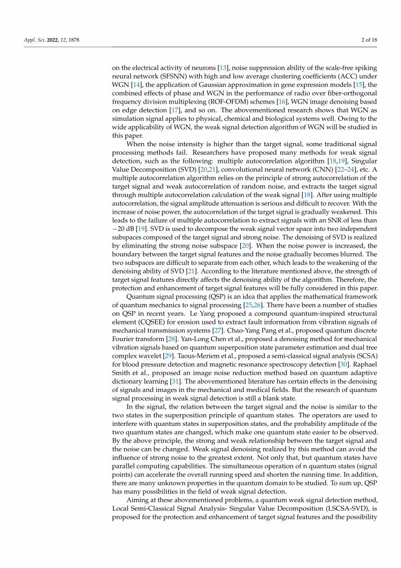
A Quantum Weak Signal Detection Method for Strengthening ...
18
Citation: Yu, T.; Li, S.; Lu, J.; Gong, S.; Gu, J.; Chen, Y. A Quantum Weak Signal Detection Method for Strengthening Target Signal Features under Strong White Gaussian Noise. Appl. Sci. 2022, 12, 1878. https:// doi.org/10.3390/app12041878 Academic Editor: Amerigo Capria Received: 20 December 2021 Accepted: 31 January 2022 Published: 11 February 2022 Publisher’s Note: MDPI stays neutral with regard to jurisdictional claims in published maps and institutional affil- iations. Copyright: © 2022 by the authors. Licensee MDPI, Basel, Switzerland. This article is an open access article distributed under the terms and conditions of the Creative Commons Attribution (CC BY) license (https:// creativecommons.org/licenses/by/ 4.0/). applied sciences Article A Quantum Weak Signal Detection Method for Strengthening Target Signal Features under Strong White Gaussian Noise Tianyi Yu 1 , Shunming Li 1 , Jiantao Lu 1, * , Siqi Gong 1 , Jianfeng Gu 2 and Yong Chen 2 1 College of Energy and Power Engineering, Nanjing University of Aeronautics and Astronautics, Nanjing 210016, China; [email protected] (T.Y.); [email protected] (S.L.); [email protected] (S.G.) 2 Jiangsu Donghua Testing Technology Co., Jingjiang 214519, China; [email protected] (J.G.); [email protected] (Y.C.) * Correspondence: [email protected]; Tel.: +86-15191452453 Abstract: As the noise power increases, the target signal features become less obvious, which leads to the failure of weak signal detection methods. To address this problem, a quantum weak signal detection method, Local Semi-Classical Signal Analysis-Singular Value Decomposition (LSCSA-SVD), for strengthening target signal features under strong white Gaussian noise is proposed. Firstly, the time domain weak signal is quantized by the Schrodinger operator and its discrete spectrum formula. Then, in the quantum domain, the later eigenvalues are used to reconstruct the time domain signal, which can protect and enhance the target signal features. Finally, the difference between signal and noise in the singular value vector is used to further extract the reconstruction signal features. In simulation, the LSCSA-SVD can accurately extract target signals from white Gaussian noise signals with a signal-to-noise ratio (SNR) of -30 dB, which is better than the comparison methods. In the experiment, the weak acceleration sensor signal and the weak signal of the test circuit are successfully extracted. The results show that the LSCSA-SVD can suppress strong noise and improve the SNR. Keywords: weak signal detection; quantum signal processing; signal features; local semi-classical signal analysis; SVD; bearing fault features 1. Introduction A weak signal is a signal in which the amplitude of the target signal is smaller than that of the noise. The signal-to-noise ratio (SNR) of a weak signal is less than 0. The target signal is completely hidden in the strong noise, whose features are fuzzy and difficult to extract [1–3]. Therefore, the key to weak signal detection (WSD) is to protect the target signal while eliminating the noise. The formula for calculating SNR in this paper is as follows [4]: SNR = 10 log Signal power Noise Power (1) With the development of integrated circuits, the precision instrument industry has a higher demand for weak signal detection [5,6]. A complex marine environment forms natural strong noise, which limits the transmission distance of sonar information [7,8]. Weak faults of rotating machinery (e.g., strong noise, early fault) are difficult to diagnose [9,10]. The above are the WSD problems that need to be solved urgently. Effectively solving WSD problems can promote the development of high and new technology. Researchers have carried out a variety of weak signal detection studies according to the needs of industries from the perspectives of the type and intensity of noise, the type of target signal, and the signal processing methods. The amplitude distribution of White Gaussian Noise (WGN) obeys Gaussian distribution, and its power spectral density obeys uniform distribution [11,12]. With components all over the spectrum, WGN is a kind of simulation noise suitable for signal-noise separation. In recent years, the influence of WGN has been considered in many fields—for example, the influence of time delay and noise Appl. Sci. 2022, 12, 1878. https://doi.org/10.3390/app12041878 https://www.mdpi.com/journal/applsci
-
Upload
khangminh22 -
Category
Documents
-
view
2 -
download
0
Transcript of A Quantum Weak Signal Detection Method for Strengthening ...
�����������������
Citation: Yu, T.; Li, S.; Lu, J.; Gong, S.;
Gu, J.; Chen, Y. A Quantum Weak
Signal Detection Method for
Strengthening Target Signal Features
under Strong White Gaussian Noise.
Appl. Sci. 2022, 12, 1878. https://
doi.org/10.3390/app12041878
Academic Editor: Amerigo Capria
Received: 20 December 2021
Accepted: 31 January 2022
Published: 11 February 2022
Publisher’s Note: MDPI stays neutral
with regard to jurisdictional claims in
published maps and institutional affil-
iations.
Copyright: © 2022 by the authors.
Licensee MDPI, Basel, Switzerland.
This article is an open access article
distributed under the terms and
conditions of the Creative Commons
Attribution (CC BY) license (https://
creativecommons.org/licenses/by/
4.0/).
applied sciences
Article
A Quantum Weak Signal Detection Method for StrengtheningTarget Signal Features under Strong White Gaussian NoiseTianyi Yu 1, Shunming Li 1, Jiantao Lu 1,* , Siqi Gong 1 , Jianfeng Gu 2 and Yong Chen 2
1 College of Energy and Power Engineering, Nanjing University of Aeronautics and Astronautics,Nanjing 210016, China; [email protected] (T.Y.); [email protected] (S.L.); [email protected] (S.G.)
2 Jiangsu Donghua Testing Technology Co., Jingjiang 214519, China; [email protected] (J.G.);[email protected] (Y.C.)
* Correspondence: [email protected]; Tel.: +86-15191452453
Abstract: As the noise power increases, the target signal features become less obvious, which leadsto the failure of weak signal detection methods. To address this problem, a quantum weak signaldetection method, Local Semi-Classical Signal Analysis-Singular Value Decomposition (LSCSA-SVD),for strengthening target signal features under strong white Gaussian noise is proposed. Firstly, thetime domain weak signal is quantized by the Schrodinger operator and its discrete spectrum formula.Then, in the quantum domain, the later eigenvalues are used to reconstruct the time domain signal,which can protect and enhance the target signal features. Finally, the difference between signal andnoise in the singular value vector is used to further extract the reconstruction signal features. Insimulation, the LSCSA-SVD can accurately extract target signals from white Gaussian noise signalswith a signal-to-noise ratio (SNR) of −30 dB, which is better than the comparison methods. In theexperiment, the weak acceleration sensor signal and the weak signal of the test circuit are successfullyextracted. The results show that the LSCSA-SVD can suppress strong noise and improve the SNR.
Keywords: weak signal detection; quantum signal processing; signal features; local semi-classicalsignal analysis; SVD; bearing fault features
1. Introduction
A weak signal is a signal in which the amplitude of the target signal is smaller thanthat of the noise. The signal-to-noise ratio (SNR) of a weak signal is less than 0. The targetsignal is completely hidden in the strong noise, whose features are fuzzy and difficult toextract [1–3]. Therefore, the key to weak signal detection (WSD) is to protect the targetsignal while eliminating the noise. The formula for calculating SNR in this paper is asfollows [4]:
SNR = 10 logSignal powerNoise Power
(1)
With the development of integrated circuits, the precision instrument industry hasa higher demand for weak signal detection [5,6]. A complex marine environment formsnatural strong noise, which limits the transmission distance of sonar information [7,8]. Weakfaults of rotating machinery (e.g., strong noise, early fault) are difficult to diagnose [9,10].The above are the WSD problems that need to be solved urgently. Effectively solving WSDproblems can promote the development of high and new technology.
Researchers have carried out a variety of weak signal detection studies according tothe needs of industries from the perspectives of the type and intensity of noise, the typeof target signal, and the signal processing methods. The amplitude distribution of WhiteGaussian Noise (WGN) obeys Gaussian distribution, and its power spectral density obeysuniform distribution [11,12]. With components all over the spectrum, WGN is a kind ofsimulation noise suitable for signal-noise separation. In recent years, the influence of WGNhas been considered in many fields—for example, the influence of time delay and noise
Appl. Sci. 2022, 12, 1878. https://doi.org/10.3390/app12041878 https://www.mdpi.com/journal/applsci
Appl. Sci. 2022, 12, 1878 2 of 18
on the electrical activity of neurons [13], noise suppression ability of the scale-free spikingneural network (SFSNN) with high and low average clustering coefficients (ACC) underWGN [14], the application of Gaussian approximation in gene expression models [15], thecombined effects of phase and WGN in the performance of radio over fiber-orthogonalfrequency division multiplexing (ROF-OFDM) schemes [16], WGN image denoising basedon edge detection [17], and so on. The abovementioned research shows that WGN assimulation signal applies to physical, chemical and biological systems well. Owing to thewide applicability of WGN, the weak signal detection algorithm of WGN will be studied inthis paper.
When the noise intensity is higher than the target signal, some traditional signalprocessing methods fail. Researchers have proposed many methods for weak signaldetection, such as the following: multiple autocorrelation algorithm [18,19], SingularValue Decomposition (SVD) [20,21], convolutional neural network (CNN) [22–24], etc. Amultiple autocorrelation algorithm relies on the principle of strong autocorrelation of thetarget signal and weak autocorrelation of random noise, and extracts the target signalthrough multiple autocorrelation calculation of the weak signal [18]. After using multipleautocorrelation, the signal amplitude attenuation is serious and difficult to recover. With theincrease of noise power, the autocorrelation of the target signal is gradually weakened. Thisleads to the failure of multiple autocorrelation to extract signals with an SNR of less than−20 dB [19]. SVD is used to decompose the weak signal vector space into two independentsubspaces composed of the target signal and strong noise. The denoising of SVD is realizedby eliminating the strong noise subspace [20]. When the noise power is increased, theboundary between the target signal features and the noise gradually becomes blurred. Thetwo subspaces are difficult to separate from each other, which leads to the weakening of thedenoising ability of SVD [21]. According to the literature mentioned above, the strength oftarget signal features directly affects the denoising ability of the algorithm. Therefore, theprotection and enhancement of target signal features will be fully considered in this paper.
Quantum signal processing (QSP) is an idea that applies the mathematical frameworkof quantum mechanics to signal processing [25,26]. There have been a number of studieson QSP in recent years. Le Yang proposed a compound quantum-inspired structuralelement (CQSEE) for erosion used to extract fault information from vibration signals ofmechanical transmission systems [27]. Chao-Yang Pang et al., proposed quantum discreteFourier transform [28]. Yan-Long Chen et al., proposed a denoising method for mechanicalvibration signals based on quantum superposition state parameter estimation and dual treecomplex wavelet [29]. Taous-Meriem et al., proposed a semi-classical signal analysis (SCSA)for blood pressure detection and magnetic resonance spectroscopy detection [30]. RaphaelSmith et al., proposed an image noise reduction method based on quantum adaptivedictionary learning [31]. The abovementioned literature has certain effects in the denoisingof signals and images in the mechanical and medical fields. But the research of quantumsignal processing in weak signal detection is still a blank state.
In the signal, the relation between the target signal and the noise is similar to thetwo states in the superposition principle of quantum states. The operators are used tointerfere with quantum states in superposition states, and the probability amplitude of thetwo quantum states are changed, which make one quantum state easier to be observed.By the above principle, the strong and weak relationship between the target signal andthe noise can be changed. Weak signal denoising realized by this method can avoid theinfluence of strong noise to the greatest extent. Not only that, but quantum states haveparallel computing capabilities. The simultaneous operation of n quantum states (signalpoints) can accelerate the overall running speed and shorten the running time. In addition,there are many unknown properties in the quantum domain to be studied. To sum up, QSPhas many possibilities in the field of weak signal detection.
Aiming at these abovementioned problems, a quantum weak signal detection method,Local Semi-Classical Signal Analysis- Singular Value Decomposition (LSCSA-SVD), isproposed for the protection and enhancement of target signal features and the possibility

Appl. Sci. 2022, 12, 1878 3 of 18
of QSP in WSD. First, LSCSA is used to enhance the features, and then SVD is used tofurther extract weak target signals. In the simulation and experiment, the effectiveness ofLSCSA-SVD is verified by comparison methods. The main contributions of this paper areas follows:
1. A quantum signal processing method, Local Semi-Classical Signal Analysis (LSCSA),has been proposed. In the LSCSA, Schrodinger operator and discrete spectrum for-mula are used to transform a time domain weak signal into a quantum domain.Then the quantum domain signal can be restored to the time domain signal by recon-structing the formula. The quantization ability of LSCSA is the basis of studying thecharacteristics of weak signals in the quantum domain.
2. The quantum domain characteristics and the singular value characteristics of weaksignals have been studied. In the quantum domain, the weak target signal mainlyexists in the later portion of the eigenvalue sequence (detail region). The weak targetsignal can be located in strong noise only by using a detailed region reconstructionsignal. The weak target signal features can be protected and strengthened by thischaracteristic. In the singular value vector, the singular values representing the weaktarget signal and the strong noise signal components can be separated as separatecoordinates. By this characteristic, noise and target signals can be accurately separated.
3. A quantum weak signal detection algorithm, the LSCSA-SVD, has been proposed inthis paper. The weak signal features are protected and strengthened by LSCSA, whichsolve the problem that SVD cannot detect weak signals when the signal features arenot obvious. SVD is used to further extract the signal features of LSCSA reconstructionsignal, which solve the problem that LSCSA cannot extract signal features directly.LSCSA-SVD can detect weak signals with low SNR and improve the SNR.
4. A clear guideline on how to select the optimal parameters of the LSCSA-SVD hasbeen given.
The rest of this paper is organized as follows: In Section 2, the theory of the QSP,the LSCSA, and the singular value characteristics of weak signals will be introduced. InSection 3, the LSCSA-SVD and how to select the optimal parameters of the LSCSA-SVD willbe introduced. In Section 4, the LSCSA-SVD will be verified on the simulation signal (SNR=−30 dB). In Section 5, the LSCSA-SVD will be analyzed experimentally with experimentaltest data. Section 6 will summarize the full text.
2. Materials and Methods2.1. Quantum Signal Processing and LSCSA
Quantum signal processing (QSP) is an idea that applies the mathematical frameworkof quantum mechanics to signal processing [32]. QSP is a natural simulation algorithmframework that builds a new algorithm based on quantum mechanics and improves theexisting algorithm. The traditional quantum computation uses the quantum effect of thephysical entity to complete the corresponding processing, but this method is limited bythe axioms and constraints of quantum physics, and it is usually difficult to realize. QSPonly uses the mathematical framework and ideas of quantum mechanics and establishescorresponding processing algorithms based on the axioms in quantum mechanics. Thismethod is not materially limited by the laws of quantum physics, and its implementationentity is an ordinary computer system [33].
In quantum mechanics, a (non-relativistic) particle in a potential state is described bya wave function ψ, whose squared absolute value |ψ|2 corresponds to the probability ofpresence of the particle [34]. The normalization of probability implies that
∫|ψ|2 = 1, and the
wave function belongs to the Hilbert space of functions with bounded integrals (L2 norm).The difficulty of QSP lies in how to combine the signal processing problem with the
mathematical framework of quantum mechanics. In QSP, the relationship between thesignal point and the time period are similar to the relationship between a particle andthe potential space, and the state of the signal point in the time period (the amplitude ofthe signal) is similar to the state of a particle in the potential space (the potential of the
Appl. Sci. 2022, 12, 1878 4 of 18
particle). Referring to the concept of wave function, Local Semi-Classical Signal Analysis(LSCSA) replaces the particle in the potential space as each point of a 1-dimensional signal,and the amplitude of each signal point is used to replace the potential of the particle. TheSchrödinger operator Φ and its discrete spectral formula are the bridge between the timedomain and the quantum domain. The calculation process is called the quantization process ofthe time-domain signal. The result/space of the computation is called the quantum domain.
In LSCSA, the Schrödinger operator Φ and its discrete spectral formula are used todecompose and reconstruct the 1-dimensional signals y. The discrete spectrum formula isas follows [35–37]:
Hh(y)Φ = − }2
2m∇2Φ−V(r)Φ, Φ ∈ H2(R) (2)
where Hh(y) is the discrete spectrum of Schrödinger operators, h̄ is the Planck constant, mis the particles in the potential of quality,52Φ is Laplacian operator, V(r) is the potentialSchrödinger operators, and H2(R) denotes the Sobolev space of order 2. In order to simplifythe formula, }2
2m is replaced with constant h2, 52Φ is replaced by the second derivativeof Schrödinger operators, and the potential of Schrödinger operators V(r) is replaced by1-dimensional vibration signal y. The simplified formula can be written as
Hh(y)Φ = −h2 d2Φdt2 − yΦ, Φ ∈ H2(R), h > 0 (3)
According to the Fourier spectrum method [38], the second derivative of Schrödingeroperators can be written as Schrödinger operators Φ multiplied by the spectrum derivativematrix D. Equation (3) can be rewritten into the following form:
Hh(y)Φ = [−h2D− diag(y)]Φ (4)
The discrete spectrum Hh(y) of Schrödinger operator is calculated by Equation (4). Theeigenvalues and eigenvectors of the spectrum are calculated by the following formula:
Hh(y)ψ(t) = λψ(t) (5)
where the eigenvalues of Hh(y) are λ and the eigenfunctions are ψ(t). The negative eigenvaluesof Hh(y) are denoted as −knh
2. The number of the negative eigenvalues is denoted as Nh. Theassociated L2-normalized eigenfunctions are denoted as ψnh, n = 1, . . . , Nh. The negativeeigenvalues and the corresponding square eigenfunctions are used for reconstruction. Thereconstructed signal is denoted as yh, and the reconstruction formula is as follows:
yh(t) = 4hNh
∑n
knhψ2nh(t), t ∈ R (6)
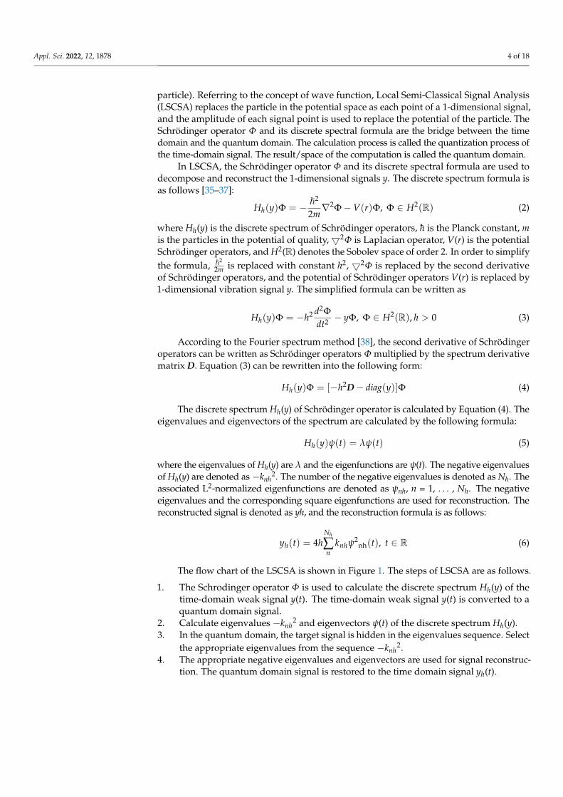
The flow chart of the LSCSA is shown in Figure 1. The steps of LSCSA are as follows.
1. The Schrodinger operator Φ is used to calculate the discrete spectrum Hh(y) of thetime-domain weak signal y(t). The time-domain weak signal y(t) is converted to aquantum domain signal.
2. Calculate eigenvalues −knh2 and eigenvectors ψ(t) of the discrete spectrum Hh(y).
3. In the quantum domain, the target signal is hidden in the eigenvalues sequence. Selectthe appropriate eigenvalues from the sequence −knh
2.4. The appropriate negative eigenvalues and eigenvectors are used for signal reconstruc-
tion. The quantum domain signal is restored to the time domain signal yh(t).
Appl. Sci. 2022, 12, 1878 5 of 18
Figure 1. Flow chart of the LSCSA.
2.2. Quantum Domain Characteristics of Weak Signal
In signal processing, it is a common method to transform the time-domain signal toother domains for analysis. The same goes for the LSCSA. In Figure 1, the time-domainweak signal y(t) is converted to a quantum-domain signal. In the quantum domain, somecharacteristics of the weak signal are different with the time domain.
In the LSCSA, parameter h plays an important role. When h decreases, Nh increasesand the reconstructed signal yh is closer to the original signal y. When the parameter hsatisfies Equation (7) and n = 1, yh = y,
4hNh
∑n=1
knh =∫ +∞
−∞y(t)dt (7)
when y∈L1/2(R),
limh→0
hNh =1π
∫ +∞
−∞
√y(t)dt (8)
It can be seen that Nh is a decreasing function of h. With the decrease of h, the number ofnegative eigenvalues and corresponding eigenfunctions increases. The negative eigenvalue−knh
2 is an ascending sequence from small to large. The front of the negative eigenvaluessequence (e.g., ψ1h, ψ2h) depicts main profile characteristics of signal y [30]. With theincrease of Nh, the eigenvalue depicts the signal y details characteristics. Eigenvectorscontain more and more information.
Based on the characteristics of the LSCSA in the quantum domain, the followinginference follows. For the ordinary signal, the noise is smaller than the target signal. In theordinary signal, the noise belongs to the detail part. By adjusting the h value, the signal canbe reconstructed with a small number of negative eigenvalues to achieve the purpose ofnoise reduction. However, for weak signals, the roles of noise and signal are reversed. Thetarget signal annihilated by strong noise is hidden in the details of the weak signal.
By using these characteristics, the target signal can be located by adjusting the h valueand using the back of the negative eigenvalue sequence. The confusion between targetsignal and strong noise can be eliminated. The interference ability of the strong noise isgreatly reduced. The target signal will not be considered as noise during signal processing,
Appl. Sci. 2022, 12, 1878 6 of 18
and can be protected by the LSCSA. After using the LSCSA, the target signal features canbe strengthened.
2.3. Singular Value Characteristics of Weak Signal
As a traditional signal processing method, Singular Value Decomposition (SVD) haslimitations [20]. When the target features in the signal are relatively obvious, SVD has abetter extraction effect on the signal features. On the contrary, SVD has little effect on signalimprovement. It means that weak signals with signal features submerged in strong noiseare not suitable for SVD to extract target signals.
It is mentioned in Section 2.1 that after using the LSCSA, the target signal can belocated in the weak signal and the target signal features can be strengthened, which ensuresthat the target characteristics have been obviously extracted from the reconstructed signalof the LSCSA. Thus, the signal can be improved by SVD after the LSCSA.
The one-dimensional vector should be constructed as a matrix before using SVD. Let theone-dimensional discrete signal Y = {y1, . . . , yk}, and the matrix construction form is as follows:
H =
y1 y2 · · · yjy2 y3 · · · yj+1...
......
...yk−j+1 yk−j+2 · · · yk
where 1 < j < k, let m = k − j + 1, H ∈ Rm×j. This matrix is the Hankel matrix. Signal Ycontains two components: target signal S and noise signal N. Target signal S contains linearsignal Sl and nonlinear periodic signal Sp (the above linear signal and nonlinear signal referto the time-domain image shape, the same as the linear function and nonlinear functionsignal in a mathematical concept). Signal Y can be expressed in the following form:
Y = S + N = Sl + Sp + N (9)
After signal Y is constructed as Hankel matrix H, it can be expressed in the following form:
H = HS + HN = Hl + Hp + HN (10)
where Hs, HN, Hl, Hp are Hankel matrices constructed by S, N, Sl, Sp, respectively.Characteristics of Hankel matrices: The next line of vectors lags only one data point
behind the previous line.Characteristics of SVD: The number of non-zero singular values generated after SVD
of the matrix is equal to the rank of the matrix.The following conclusions can be drawn from the above two characteristics:
1. In the matrix Hl constructed by linear signal Sl, each row is linearly dependent. So therank of the matrix Hl r = 1, and the singular value vector can be expressed as σ(Hl) =(σl, 0, . . . , 0).
2. Due to the periodicity of the nonlinear periodic signal Sp, denoted by period T, thevector of the first T row of the matrix Hp is linearly independent, and the other linesare linearly related to the vector of the first T row. Therefore, the rank of the matrixHp r < min(m,j), and the singular value vector can be expressed as σ(Hp) = (σp1, σp2,. . . , σpr, 0, . . . , 0).
3. The random noise signal N is irrelevant at every moment. Therefore, each row of theconstructed matrix HN is unrelated, so the rank of the matrix HN r = min(m,j). Thesingular value vector can be expressed as σ(HN) = (σn1, σn2, . . . , σnr).
Reference [39] points out that when min(m,j) is maximized, the singular value ofmatrix H has a relationship with the singular value of matrix HN, Hl, Hp, as follows [39]:
σ(H) = σ(Hl + Hp + HN
)≈(σl , σp1, σp2, . . . , σpr, σn1, . . . , σnr
)(11)

Appl. Sci. 2022, 12, 1878 7 of 18
It can be seen that, in the total singular value vector of mixed signals, the singularvalues representing the target signal and the noise signal components can be separatedas separate coordinates. Moreover, the singular value of the noise component will beseparated into the posterior coordinates of the total vector. Therefore, the signal noisereduction can be achieved by selecting the appropriate singular value and its correspondingvector for SVD reconstruction.
3. LSCSA-SVD
According to the theory in Section 2, a novel quantum weak signal detection method,LSCSA-SVD, is proposed. The steps of LSCSA-SVD (Algorithm 1) are as follows, and theflow diagram is shown in Figure 2.
Algorithm 1. LSCSA-SVD.
Input: y(t), Φ, h, k1: Calculate the discrete spectrum Hh(y) of Schrödinger operator Φ and weak signal y(t).2: Calculate the eigenvalue λ and the eigenfunctions ψ(t) of spectrum Hh(y).3: Using Equation (12), the negative eigenvalues of k to Nh and their associated L2-normalizedeigenfunctions are reconstructed to yh(t).4: Reconstructed signal yh(t) constructs Hankel matrix H.5: Calculate the singular values of the Hankel matrix H.6: The nonlinear periodic component of singular value vector is selected for SVD reconstruction toobtain the matrix H*.7: The first row and last column of the matrix H* are restored to the 1-dimensional signal y*(t).y*(t) is the weak target signal.Output: y*(t).
Figure 2. Flow diagram of LSCSA-SVD.
Appl. Sci. 2022, 12, 1878 8 of 18
yh(t) = 4hNh
∑n=k
knhψ2nh(t), t ∈ R (12)
There are two important parameters, h and k, in the LSCSA-SVD. They can be selectedin the following manner:
1. Parameter h
Standard 1: Nh = length (y(t)).Standard 2: On the premise of satisfying Standard 1, the parameter h should be as
large as possible.From Equation (4), it can be seen that the dimension of discrete spectrum Hh(y) is equal
to the length of signal y, and Nh ≤ length (y(t)). In order to obtain as many detailed featuresin the reconstructed signal as possible, as many negative eigenvalues as possible are needed.So Nh = length (y(t)) (Standard 1). While satisfying Standard 1, if the parameter h is toosmall, the reconstructed signal will be seriously distorted. Therefore, the parameter h needsto be as large as possible (Standard 2). Parameter h can be obtained through the loop onthe left of Figure 2.
2. Parameter k
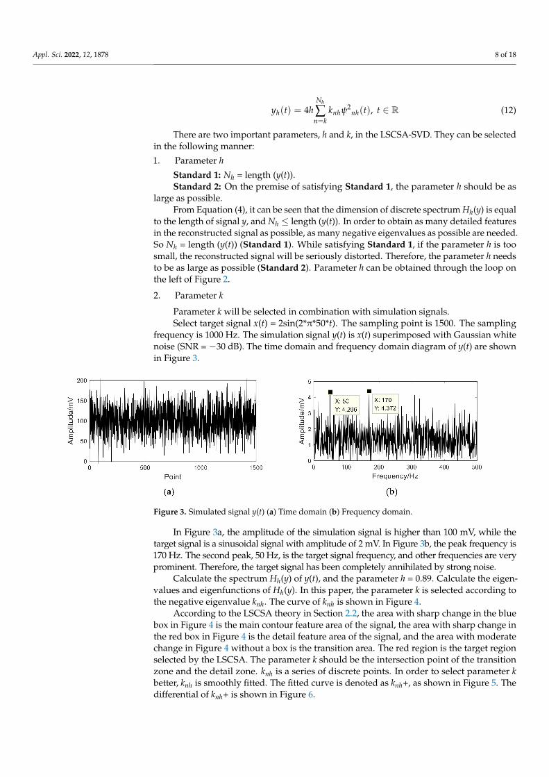
Parameter k will be selected in combination with simulation signals.Select target signal x(t) = 2sin(2*π*50*t). The sampling point is 1500. The sampling
frequency is 1000 Hz. The simulation signal y(t) is x(t) superimposed with Gaussian whitenoise (SNR = −30 dB). The time domain and frequency domain diagram of y(t) are shownin Figure 3.
Figure 3. Simulated signal y(t) (a) Time domain (b) Frequency domain.
In Figure 3a, the amplitude of the simulation signal is higher than 100 mV, while thetarget signal is a sinusoidal signal with amplitude of 2 mV. In Figure 3b, the peak frequency is170 Hz. The second peak, 50 Hz, is the target signal frequency, and other frequencies are veryprominent. Therefore, the target signal has been completely annihilated by strong noise.
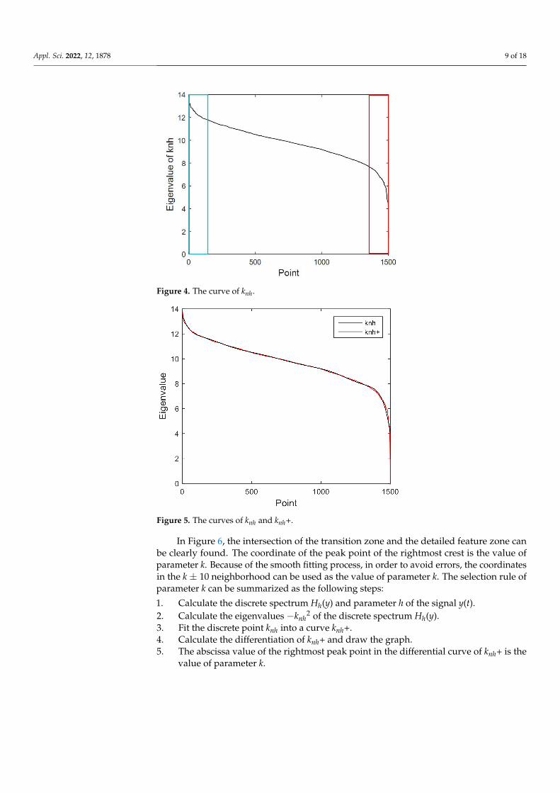
Calculate the spectrum Hh(y) of y(t), and the parameter h = 0.89. Calculate the eigen-values and eigenfunctions of Hh(y). In this paper, the parameter k is selected according tothe negative eigenvalue knh. The curve of knh is shown in Figure 4.
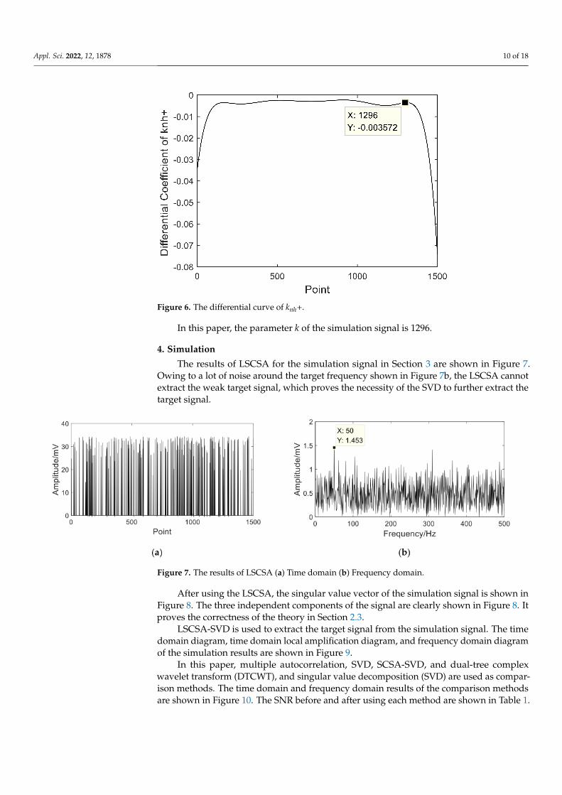
According to the LSCSA theory in Section 2.2, the area with sharp change in the bluebox in Figure 4 is the main contour feature area of the signal, the area with sharp change inthe red box in Figure 4 is the detail feature area of the signal, and the area with moderatechange in Figure 4 without a box is the transition area. The red region is the target regionselected by the LSCSA. The parameter k should be the intersection point of the transitionzone and the detail zone. knh is a series of discrete points. In order to select parameter kbetter, knh is smoothly fitted. The fitted curve is denoted as knh+, as shown in Figure 5. Thedifferential of knh+ is shown in Figure 6.
Appl. Sci. 2022, 12, 1878 9 of 18
Figure 4. The curve of knh.
Figure 5. The curves of knh and knh+.
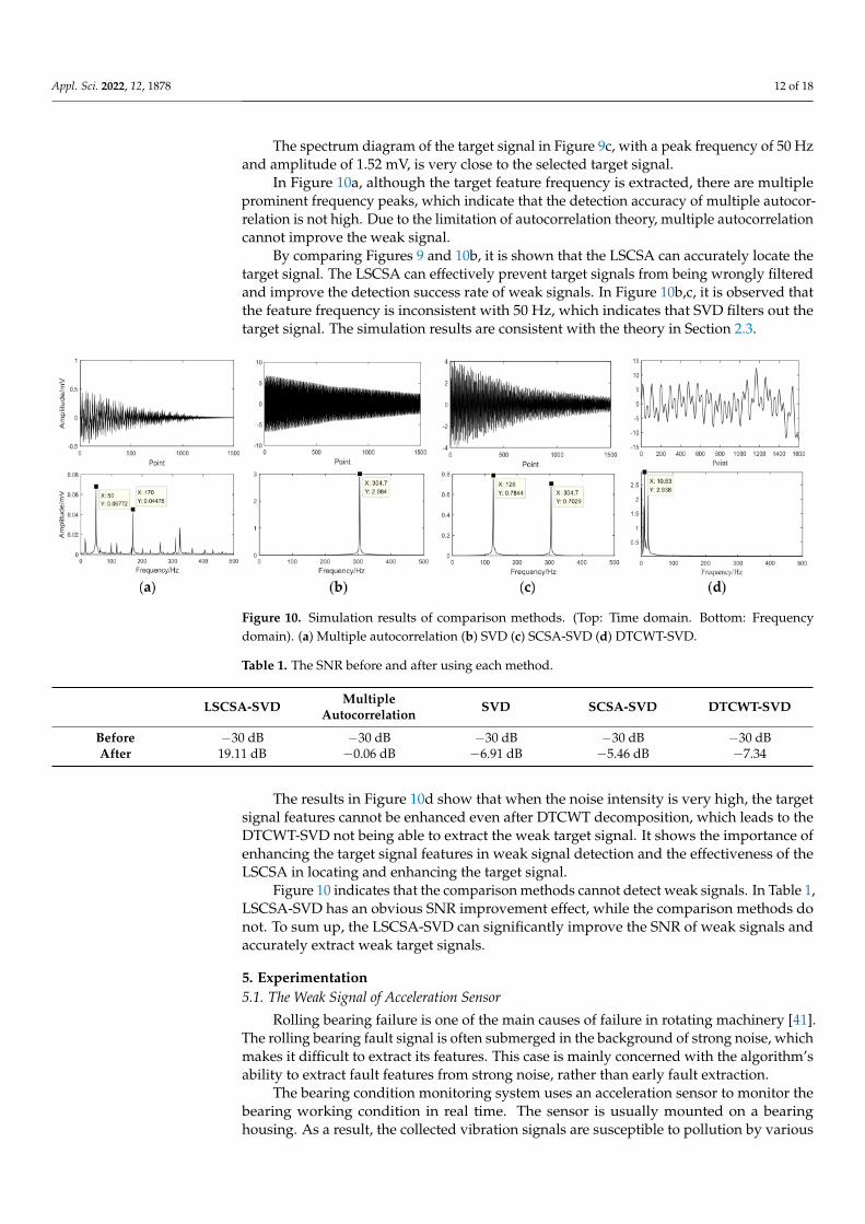
In Figure 6, the intersection of the transition zone and the detailed feature zone canbe clearly found. The coordinate of the peak point of the rightmost crest is the value ofparameter k. Because of the smooth fitting process, in order to avoid errors, the coordinatesin the k ± 10 neighborhood can be used as the value of parameter k. The selection rule ofparameter k can be summarized as the following steps:
1. Calculate the discrete spectrum Hh(y) and parameter h of the signal y(t).2. Calculate the eigenvalues −knh
2 of the discrete spectrum Hh(y).3. Fit the discrete point knh into a curve knh+.4. Calculate the differentiation of knh+ and draw the graph.5. The abscissa value of the rightmost peak point in the differential curve of knh+ is the
value of parameter k.
Appl. Sci. 2022, 12, 1878 10 of 18
Figure 6. The differential curve of knh+.
In this paper, the parameter k of the simulation signal is 1296.
4. Simulation
The results of LSCSA for the simulation signal in Section 3 are shown in Figure 7.Owing to a lot of noise around the target frequency shown in Figure 7b, the LSCSA cannotextract the weak target signal, which proves the necessity of the SVD to further extract thetarget signal.
Figure 7. The results of LSCSA (a) Time domain (b) Frequency domain.
After using the LSCSA, the singular value vector of the simulation signal is shown inFigure 8. The three independent components of the signal are clearly shown in Figure 8. Itproves the correctness of the theory in Section 2.3.
LSCSA-SVD is used to extract the target signal from the simulation signal. The timedomain diagram, time domain local amplification diagram, and frequency domain diagramof the simulation results are shown in Figure 9.
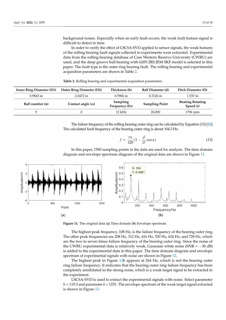
In this paper, multiple autocorrelation, SVD, SCSA-SVD, and dual-tree complexwavelet transform (DTCWT), and singular value decomposition (SVD) are used as compar-ison methods. The time domain and frequency domain results of the comparison methodsare shown in Figure 10. The SNR before and after using each method are shown in Table 1.

Appl. Sci. 2022, 12, 1878 11 of 18
Figure 8. Singular value vector after using the LSCSA.
Multiple autocorrelation: Multiple autocorrelation is a traditional weak signal detec-tion method. This example is used to test the performance of the LSCSA-SVD [18].
SVD: SVD is also a traditional weak signal detection algorithm [21]. This example notonly verifies the performance of the LSCSA-SVD, but also proves the necessity of the LSCSA.
SCSA-SVD: This example is used to prove the necessity of the LSCSA.DTCWT-SVD: DTCWT is used to carry out multilevel decomposition and purifying for
an acceleration series. SVD is used to de-noise each layer of wavelet in the decompositionprocess. The decomposed signals are filtered and SVD denoised to detect weak signals [40].
Figure 9. Simulation results of LSCSA-SVD (a) Time domain (b) Local amplification diagram of (a,c)Frequency domain.
Appl. Sci. 2022, 12, 1878 12 of 18
The spectrum diagram of the target signal in Figure 9c, with a peak frequency of 50 Hzand amplitude of 1.52 mV, is very close to the selected target signal.
In Figure 10a, although the target feature frequency is extracted, there are multipleprominent frequency peaks, which indicate that the detection accuracy of multiple autocor-relation is not high. Due to the limitation of autocorrelation theory, multiple autocorrelationcannot improve the weak signal.
By comparing Figures 9 and 10b, it is shown that the LSCSA can accurately locate thetarget signal. The LSCSA can effectively prevent target signals from being wrongly filteredand improve the detection success rate of weak signals. In Figure 10b,c, it is observed thatthe feature frequency is inconsistent with 50 Hz, which indicates that SVD filters out thetarget signal. The simulation results are consistent with the theory in Section 2.3.
Figure 10. Simulation results of comparison methods. (Top: Time domain. Bottom: Frequencydomain). (a) Multiple autocorrelation (b) SVD (c) SCSA-SVD (d) DTCWT-SVD.
Table 1. The SNR before and after using each method.
LSCSA-SVD MultipleAutocorrelation SVD SCSA-SVD DTCWT-SVD
Before −30 dB −30 dB −30 dB −30 dB −30 dBAfter 19.11 dB −0.06 dB −6.91 dB −5.46 dB −7.34
The results in Figure 10d show that when the noise intensity is very high, the targetsignal features cannot be enhanced even after DTCWT decomposition, which leads to theDTCWT-SVD not being able to extract the weak target signal. It shows the importance ofenhancing the target signal features in weak signal detection and the effectiveness of theLSCSA in locating and enhancing the target signal.
Figure 10 indicates that the comparison methods cannot detect weak signals. In Table 1,LSCSA-SVD has an obvious SNR improvement effect, while the comparison methods donot. To sum up, the LSCSA-SVD can significantly improve the SNR of weak signals andaccurately extract weak target signals.
5. Experimentation5.1. The Weak Signal of Acceleration Sensor
Rolling bearing failure is one of the main causes of failure in rotating machinery [41].The rolling bearing fault signal is often submerged in the background of strong noise, whichmakes it difficult to extract its features. This case is mainly concerned with the algorithm’sability to extract fault features from strong noise, rather than early fault extraction.
The bearing condition monitoring system uses an acceleration sensor to monitor thebearing working condition in real time. The sensor is usually mounted on a bearinghousing. As a result, the collected vibration signals are susceptible to pollution by various
Appl. Sci. 2022, 12, 1878 13 of 18
background noises. Especially when an early fault occurs, the weak fault feature signal isdifficult to detect in time.
In order to verify the effect of LSCSA-SVD applied to sensor signals, the weak featuresof the rolling bearing fault signals collected in experiments were extracted. Experimentaldata from the rolling bearing database of Case Western Reserve University (CWRU) areused, and the deep groove ball bearing with 6205-2RS JEM SKF model is selected in thispaper. The fault type is the outer ring bearing fault. The rolling bearing and experimentalacquisition parameters are shown in Table 2.
Table 2. Rolling bearing and experimental acquisition parameters.
Inner Ring Diameter (D1) Outer Ring Diameter (D2) Thickness (h) Ball Diameter (d) Pitch Diameter (D)
0.9843 in 2.0472 in 0.5906 in 0.3126 in 1.537 in
Ball number (n) Contact angle (α) SamplingFrequency (Fs) Sampling Point Bearing Rotating
Speed (r)
9 0 12 kHz 20,000 1796 rpm
The failure frequency of the rolling bearing outer ring can be calculated by Equation (13) [42].The calculated fault frequency of the bearing outer ring is about 104.3 Hz.
f =rn
120(1− d
Dcos α) (13)
In this paper, 1500 sampling points in the data are used for analysis. The time domaindiagram and envelope spectrum diagram of the original data are shown in Figure 11.
Figure 11. The original data (a) Time domain (b) Envelope spectrum.
The highest peak frequency, 108 Hz, is the failure frequency of the bearing outer ring.The other peak frequencies are 208 Hz, 312 Hz, 416 Hz, 520 Hz, 624 Hz, and 728 Hz, whichare the two to seven times failure frequency of the bearing outer ring. Since the noise ofthe CWRU experimental data is relatively weak, Gaussian white noise (SNR = −30 dB)is added to the experimental data in this paper. The time domain diagram and envelopespectrum of experimental signals with noise are shown in Figure 12.
The highest peak in Figure 12b appears at 264 Hz, which is not the bearing outerring failure frequency. It indicates that the bearing outer ring failure frequency has beencompletely annihilated in the strong noise, which is a weak target signal to be extracted inthe experiment.
LSCSA-SVD is used to extract the experimental signals with noise. Select parameterh = 119.3 and parameter k = 1253. The envelope spectrum of the weak target signal extractedis shown in Figure 13.
Appl. Sci. 2022, 12, 1878 14 of 18
Figure 12. Experimental signals with noise (a) Time domain (b) Envelope spectrum.
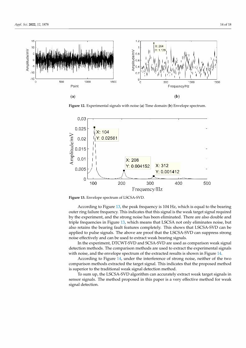
Figure 13. Envelope spectrum of LSCSA-SVD.
According to Figure 13, the peak frequency is 104 Hz, which is equal to the bearingouter ring failure frequency. This indicates that this signal is the weak target signal requiredby the experiment, and the strong noise has been eliminated. There are also double andtriple frequencies in Figure 13, which means that LSCSA not only eliminates noise, butalso retains the bearing fault features completely. This shows that LSCSA-SVD can beapplied to pulse signals. The above are proof that the LSCSA-SVD can suppress strongnoise effectively and can be used to extract weak bearing signals.
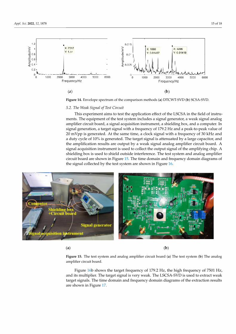
In the experiment, DTCWT-SVD and SCSA-SVD are used as comparison weak signaldetection methods. The comparison methods are used to extract the experimental signalswith noise, and the envelope spectrum of the extracted results is shown in Figure 14.
According to Figure 14, under the interference of strong noise, neither of the twocomparison methods extracted the target signal. This indicates that the proposed methodis superior to the traditional weak signal detection method.
To sum up, the LSCSA-SVD algorithm can accurately extract weak target signals insensor signals. The method proposed in this paper is a very effective method for weaksignal detection.
Appl. Sci. 2022, 12, 1878 15 of 18
Figure 14. Envelope spectrum of the comparison methods (a) DTCWT-SVD (b) SCSA-SVD.
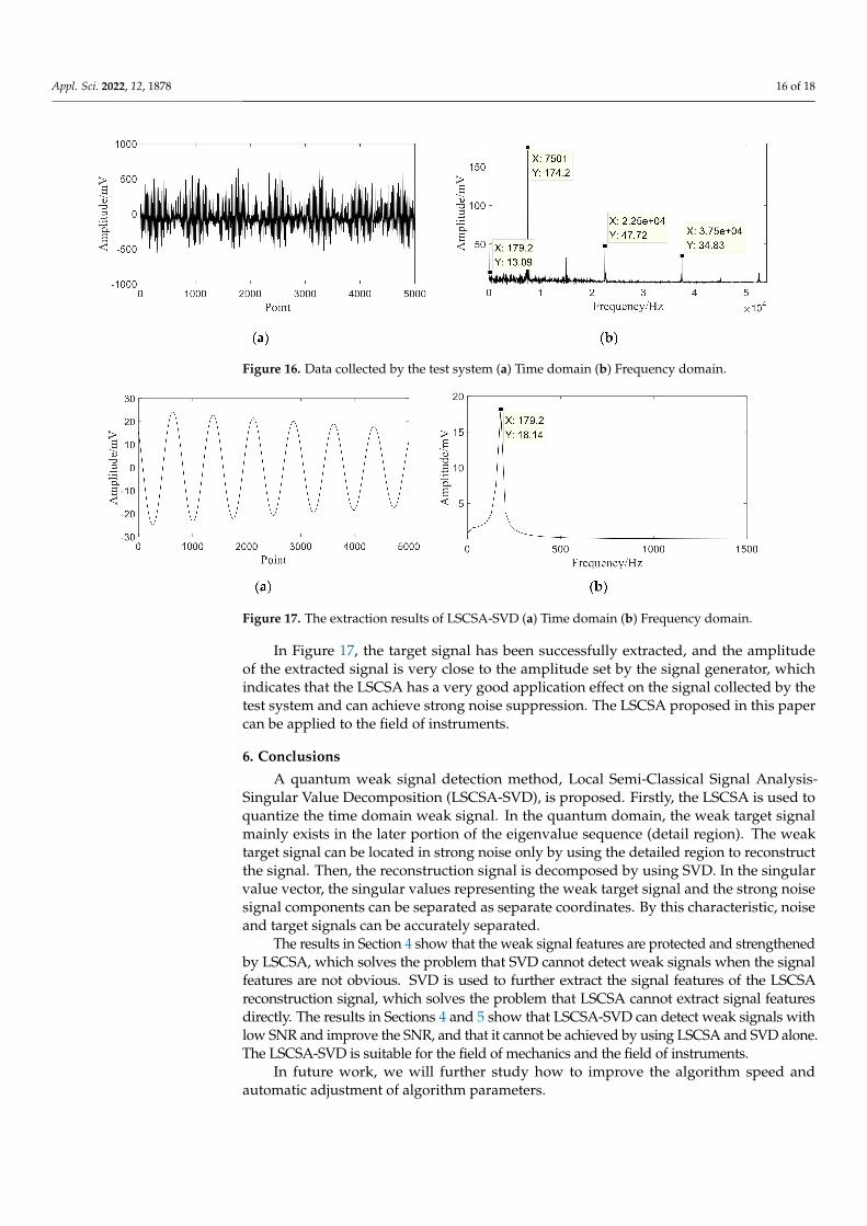
5.2. The Weak Signal of Test Circuit
This experiment aims to test the application effect of the LSCSA in the field of instru-ments. The equipment of the test system includes a signal generator, a weak signal analogamplifier circuit board, a signal acquisition instrument, a shielding box, and a computer. Insignal generation, a target signal with a frequency of 179.2 Hz and a peak-to-peak value of20 mVpp is generated. At the same time, a clock signal with a frequency of 30 kHz anda duty cycle of 10% is generated. The target signal is attenuated by a large capacitor, andthe amplification results are output by a weak signal analog amplifier circuit board. Asignal acquisition instrument is used to collect the output signal of the amplifying chip. Ashielding box is used to shield outside interference. The test system and analog amplifiercircuit board are shown in Figure 15. The time domain and frequency domain diagrams ofthe signal collected by the test system are shown in Figure 16.
Figure 15. The test system and analog amplifier circuit board (a) The test system (b) The analogamplifier circuit board.
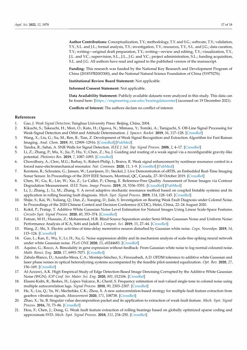
Figure 16b shows the target frequency of 179.2 Hz, the high frequency of 7501 Hz,and its multiplier. The target signal is very weak. The LSCSA-SVD is used to extract weaktarget signals. The time domain and frequency domain diagrams of the extraction resultsare shown in Figure 17.
Appl. Sci. 2022, 12, 1878 16 of 18
Figure 16. Data collected by the test system (a) Time domain (b) Frequency domain.
Figure 17. The extraction results of LSCSA-SVD (a) Time domain (b) Frequency domain.
In Figure 17, the target signal has been successfully extracted, and the amplitudeof the extracted signal is very close to the amplitude set by the signal generator, whichindicates that the LSCSA has a very good application effect on the signal collected by thetest system and can achieve strong noise suppression. The LSCSA proposed in this papercan be applied to the field of instruments.
6. Conclusions
A quantum weak signal detection method, Local Semi-Classical Signal Analysis-Singular Value Decomposition (LSCSA-SVD), is proposed. Firstly, the LSCSA is used toquantize the time domain weak signal. In the quantum domain, the weak target signalmainly exists in the later portion of the eigenvalue sequence (detail region). The weaktarget signal can be located in strong noise only by using the detailed region to reconstructthe signal. Then, the reconstruction signal is decomposed by using SVD. In the singularvalue vector, the singular values representing the weak target signal and the strong noisesignal components can be separated as separate coordinates. By this characteristic, noiseand target signals can be accurately separated.
The results in Section 4 show that the weak signal features are protected and strengthenedby LSCSA, which solves the problem that SVD cannot detect weak signals when the signalfeatures are not obvious. SVD is used to further extract the signal features of the LSCSAreconstruction signal, which solves the problem that LSCSA cannot extract signal featuresdirectly. The results in Sections 4 and 5 show that LSCSA-SVD can detect weak signals withlow SNR and improve the SNR, and that it cannot be achieved by using LSCSA and SVD alone.The LSCSA-SVD is suitable for the field of mechanics and the field of instruments.
In future work, we will further study how to improve the algorithm speed andautomatic adjustment of algorithm parameters.
Appl. Sci. 2022, 12, 1878 17 of 18
Author Contributions: Conceptualization, T.Y.; methodology, T.Y. and S.G.; software, T.Y.; validation,T.Y., S.L. and J.L.; formal analysis, T.Y.; investigation, T.Y.; resources, T.Y., S.L. and J.G.; data curation,T.Y.; writing—original draft preparation, T.Y.; writing—review and editing, T.Y.; visualization, T.Y.,J.L. and Y.C.; supervision, S.L., J.L., J.G. and Y.C.; project administration, S.L.; funding acquisition,S.L. and J.G. All authors have read and agreed to the published version of the manuscript.
Funding: This research was funded by the National Key Research and Development Program ofChina (2018YFB2003300), and the National Natural Science Foundation of China (51975276).
Institutional Review Board Statement: Not applicable.
Informed Consent Statement: Not applicable.
Data Availability Statement: Publicly available datasets were analyzed in this study. This data canbe found here: [https://engineering.case.edu/bearingdatacenter] (accessed on 19 December 2021).
Conflicts of Interest: The authors declare no conflict of interest.
References1. Gao, J. Weak Signal Detection; Tsinghua University Press: Beijing, China, 2004.2. Kikuchi, S.; Takeuchi, H.; Mori, O.; Kato, H.; Ogawa, N.; Mimasu, Y.; Tomiki, A.; Taniguchi, S. Off-Line Signal Processing for
Weak-Signal Detection and Orbit and Attitude Determination. J. Spacecr. Rocket. 2019, 56, 117–128. [CrossRef]3. Wang, X.; Liu, G.; Xu, M.; Ren, B.; Tian, Z. Development of Weak Signal Recognition and Extraction Algorithm for Fast Raman
Imaging. Anal. Chem. 2019, 91, 12909–12916. [CrossRef] [PubMed]4. Tandra, R.; Sahai, A. SNR Walls for Signal Detection. IEEE J. Sel. Top. Signal Process. 2008, 2, 4–17. [CrossRef]5. Li, Z.; Zhang, P.; Mu, X.; Jia, P.; Hu, Y.; Chen, Z.; Xu, J. Guiding and routing of a weak signal via a reconfigurable gravity-like
potential. Photonics Res. 2019, 7, 1087–1093. [CrossRef]6. Chowdhury, A.; Clerc, M.G.; Barbay, S.; Robert-Philip, I.; Braive, R. Weak signal enhancement by nonlinear resonance control in a
forced nano-electromechanical resonator. Nat. Commun. 2020, 11, 1–9. [CrossRef] [PubMed]7. Kerstens, R.; Schouten, G.; Jansen, W.; Laurijssen, D.; Steckel, J. Live Demonstration of eRTIS, an Embedded Real-Time Imaging
Sonar Sensor. In Proceedings of the 2019 IEEE Sensors, Montreal, QC, Canada, 27–30 October 2019. [CrossRef]8. Chen, W.; Gu, K.; Lin, W.; Xia, Z.; Le Callet, P.; Cheng, E. Reference-Free Quality Assessment of Sonar Images via Contour
Degradation Measurement. IEEE Trans. Image Process. 2019, 28, 5336–5351. [CrossRef] [PubMed]9. Li, J.; Zhang, J.; Li, M.; Zhang, Y. A novel adaptive stochastic resonance method based on coupled bistable systems and its
application in rolling bearing fault diagnosis. Mech. Syst. Signal Process. 2019, 114, 128–145. [CrossRef]10. Shijie, S.; Kai, W.; Xuliang, Q.; Dan, Z.; Xueqing, D.; Jiale, S. Investigation on Bearing Weak Fault Diagnosis under Colored Noise.
In Proceedings of the 2020 Chinese Control and Decision Conference (CCDC), Hefei, China, 22–24 August 2020.11. Kokil, P.; Pratap, T. Additive White Gaussian Noise Level Estimation for Natural Images Using Linear Scale-Space Features.
Circuits Syst. Signal Process. 2020, 40, 353–374. [CrossRef]12. Fatnan, M.H.; Hussain, Z.; Mohammed, H.R. Blind Source Separation under Semi-White Gaussian Noise and Uniform Noise:
Performance Analysis of ICA, Sobi and JadeR. J. Comput. Sci. 2019, 15, 27–44. [CrossRef]13. Wang, Z.; Shi, X. Electric activities of time-delay memristive neuron disturbed by Gaussian white noise. Cogn. Neurodyn. 2019, 14,
115–124. [CrossRef]14. Guo, L.; Kan, E.; Wu, Y.; Lv, H.; Xu, G. Noise suppression ability and its mechanism analysis of scale-free spiking neural network
under white Gaussian noise. PLoS ONE 2020, 15, e0244683. [CrossRef]15. Aquino, G.; Rocco, A. Bimodality in gene expression without feedback: From Gaussian white noise to log-normal coloured noise.
Math. Biosci. Eng. 2020, 17, 6993–7071. [CrossRef]16. Zabala-Blanco, D.; Azurdia-Meza, C.A.; Montejo-Sánchez, S.; Firoozabadi, A.D. OFDM tolerance to additive white Gaussian and
laser phase noises in optical heterodyning systems accompanied by the feasible pilot-assisted equalization. Opt. Rev. 2020, 27,156–169. [CrossRef]
17. Al-Azzawi, A.K. High Empirical Study of Edge Detection-Based Image Denoising Corrupted by the Additive White GaussianNoise (WGN). IOP Conf. Ser. Mater. Sci. Eng. 2020, 881, 012106. [CrossRef]
18. Elasmi-Ksibi, R.; Besbes, H.; López-Valcarce, R.; Cherif, S. Frequency estimation of real-valued single-tone in colored noise usingmultiple autocorrelation lags. Signal Process. 2010, 90, 2303–2307. [CrossRef]
19. He, X.; Liu, Q.; Yu, W.; Mechefske, C.K.; Zhou, X. A new autocorrelation-based strategy for multiple fault feature extraction fromgearbox vibration signals. Measurement 2020, 171, 108738. [CrossRef]
20. Zhao, X.; Ye, B. Singular value decomposition packet and its application to extraction of weak fault feature. Mech. Syst. SignalProcess. 2016, 70, 73–86. [CrossRef]
21. Hou, F.; Chen, J.; Dong, G. Weak fault feature extraction of rolling bearings based on globally optimized sparse coding andapproximate SVD. Mech. Syst. Signal Process. 2018, 111, 234–250. [CrossRef]

Appl. Sci. 2022, 12, 1878 18 of 18
22. Lei, Y.; Yang, B.; Jiang, X.; Jia, F.; Li, N.; Nandi, A.K. Applications of machine learning to machine fault diagnosis: A review androadmap. Mech. Syst. Signal Process. 2020, 138, 106587. [CrossRef]
23. Sun, J.; Yan, C.; Wen, J. Intelligent Bearing Fault Diagnosis Method Combining Compressed Data Acquisition and Deep Learning.IEEE Trans. Instrum. Meas. 2017, 67, 185–195. [CrossRef]
24. Yildirim, A.; Kiranyaz, S. 1D Convolutional Neural Networks Versus Automatic Classifiers for Known LPI Radar Signals UnderWhite Gaussian Noise. IEEE Access 2020, 8, 180534. [CrossRef]
25. Eldar, Y.C.; Oppenheim, A.V. Quantum signal processing. IEEE Signal Process. Mag. 2001, 19, 12–32. [CrossRef]26. Chapeau-Blondeau, F.; Belin, E. Fourier-transform quantum phase estimation with quantum phase noise. Signal Process. 2019,
170, 107441. [CrossRef]27. Le, Y. Vibration Signal Processing of Transmission System Based on Quantum Inspired Mathematical Morphology. Mech. Transm.
2017, 41, 189–193.28. Pang, C.Y.; Hu, B.Q. Quantum Discrete Fourier Transform with Classical Output for Signal Processing. Physics 2007, 101, 309–332.29. Yanlong, C.; Peilin, Z.; Huaiguang, W. Mechanical Vibration Signal Denoising Method Based on Quantum Superposition State
Parameter Estimation. Shock. Vib. 2014, 33, 143–147.30. Laleg-Kirati, T.M.; Crépeau, E.; Sorine, M. Semi-classical signal analysis. Math. Control. Signals Syst. 2013, 25, 37–61. [CrossRef]31. Smith, R.; Basarab, A.; Georgeot, B.; Kouame, D. Adaptive transform via quantum signal processing: Application to signal and
image denoising. In Proceedings of the 2018 25th IEEE International Conference on Image Processing (ICIP), Athens, Greece,7–10 October 2018; pp. 1523–1527. [CrossRef]
32. Low, G.H.; Chuang, I.L. Optimal Hamiltonian Simulation by Quantum Signal Processing. Phys. Rev. Lett. 2016, 118, 010501.[CrossRef]
33. Nieto-Chaupis, H. Quantum Effects without Quantum Fields: Feynman’s Amplitudes in Classical Electrodynamics. In Proceed-ings of the 2019 IEEE 2nd British and Irish Conference on Optics and Photonics (BICOP), London, UK, 11–13 December 2019; pp.1–4. [CrossRef]
34. Wen, T.; Yan, J.; Huang, D.; Lu, K.; Deng, C.; Zeng, T.; Yu, S.; He, Z. Feature Extraction of Electronic Nose Signals UsingQPSO-Based Multiple KFDA Signal Processing. Sensors 2018, 18, 388. [CrossRef]
35. Bhaduri, S.; Chahid, A.; Achten, E.; Laleg-Kirati, T.M.; Serrai, H. SCSA based MATLAB pre-processing toolbox for 1H MRspectroscopic water sup-pression and denoising. Inform. Med. Unlocked 2020, 18, 100294. [CrossRef]
36. Laleg-Kirati, T.M.; Zhang, J.; Achten, E.; Serrai, H. Spectral data de-noising using semi-classical signal analysis: Application tolo-calized MRS. NMR Biomed. 2016, 29, 1477–1485. [CrossRef]
37. Chahid, A.; Serrai, H.; Achten, E.; Laleg-Kirati, T.M. A New ROI-Based performance evaluation method for image denoising usingthe Squared Eigenfunctions of the Schrödinger Operator. In Proceedings of the 2018 40th Annual International Conference of theIEEE Engineering in Medicine and Biology Society (EMBC), Honolulu, HI, USA, 18–21 July 2018; Volume 2018, pp. 5579–5582.[CrossRef]
38. Zhang, X. Efficient Solution of Matlab Differential Equation: Principle and Implementation of Spectral Method; Mechanical IndustryPress: Beijing, China, 2016.
39. Zhao, X.; Ye, B.; Chen, J. Weak fault Feature Extraction Method based on Wavelet singular value Decomposition Differentialspectrum. J. Mech. Eng. 2012, 7, 37–48. [CrossRef]
40. Wang, N.F.; Jiang, D.X.; Yang, W.G. Dual-Tree Complex Wavelet Transform and SVD-Based Acceleration Signals Denoising andits Application in Fault Features Enhancement for Wind Turbine. J. Vib. Eng. Technol. 2019, 7, 311–320. [CrossRef]
41. Wang, H.; Chen, J.; Dong, G. Feature extraction of rolling bearing’s early weak fault based on EEMD and tunable Q-factor wavelettransform. Mech. Syst. Signal Process. 2014, 48, 103–119. [CrossRef]
42. Zhao, X.; Ye, B. Similarity of signal processing effect between Hankel matrix-based SVD and wavelet transform and its mechanismanalysis. Mech. Syst. Signal Process. 2009, 23, 1062–1075. [CrossRef]