A Prognostic Framework for Health Management of Coupled Systems

Chaitanya Sankavaram, Anuradha Kodali, Krishna Pattipati, Bing Wang Department of Electrical and Computer Engineering,

University of Connecticut, Storrs, CT 06269, USA

{krishna, chaitanya}@engr.uconn.edu

Mohammad S. Azam Member, Technical Staff, Qualtech Systems, Inc.,

99 East River Drive, East Hatford, CT 06108, USA

Satnam Singh Senior Researcher, Diagnosis and Prognosis Group,

GM India Science Lab, ITPL, Whitefield, Bangalore, Karnataka 560066, India

Abstract— This paper describes a unified data-driven prognostic framework that combines failure time data, static parameter data and dynamic (time-series) data. The approach employs Cox proportional hazards model (Cox PHM) and soft dynamic multiple fault diagnosis algorithm (DMFD) for inferring the degraded state trajectories of components and to estimate their remaining useful life (RUL). This framework takes into account the cross-subsystem fault propagation, a case prevalent in any networked and embedded system. The key idea is to use Cox proportional hazards model to estimate the survival functions of error codes and symptoms (soft test outcomes/prognostic indicators) from failure time data and static parameter data, and use them to infer the survival functions of components via a soft DMFD algorithm. The average remaining useful life and its higher-order central moments (e.g., variance, skewness, kurtosis) can be estimated from these component survival functions. The proposed prognostic framework has the potential to be applicable to a wide variety of systems, ranging from automobiles to aerospace systems.

Keywords: proportional hazard model (PHM), dynamic multiple fault diagnosis (DMFD), diagnostic trouble codes (DTCs), parameter identifiers (PIDs), repair codes (LCs)

I. INTRODUCTION The rapid advances in electronics, computing, and

communication technologies have resulted in complex embedded and ultra-integrated systems (e.g., automotive, aerospace and nuclear systems). Conventional maintenance strategies, such as reactive and preventive maintenance, are inadequate in fulfilling the needs of high-availability in these systems. Consequently, a continuous monitoring and early warning capability that detects, isolates and estimates the component failures (viz., fault diagnosis and prognosis) over time is required to minimize downtime, operational costs, and improve resource management via condition-based maintenance. Failure prognosis, an add-on capability to diagnosis, involves forecasting system degradation and time-to-failure (remaining useful life) based on “state awareness” gleaned from monitored data, for example, parameters

collected from various sensors, such as vehicle speed, individual wheel speeds, yaw rate, master brake cylinder pressure, and so on.

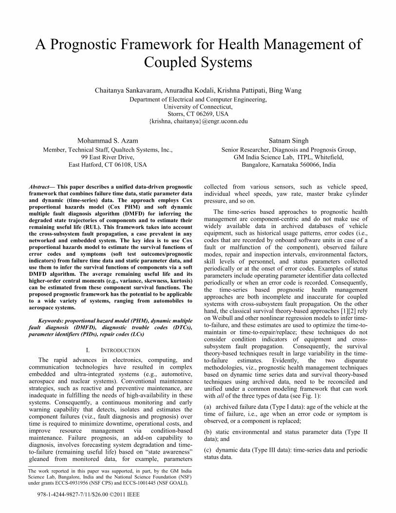
The time-series based approaches to prognostic health management are component-centric and do not make use of widely available data in archived databases of vehicle equipment, such as historical usage patterns, error codes (i.e., codes that are recorded by onboard software units in case of a fault or malfunction of the component), observed failure modes, repair and inspection intervals, environmental factors, skill levels of personnel, and status parameters collected periodically or at the onset of error codes. Examples of status parameters include operating parameter identifier data collected periodically or when an error code is recorded. Consequently, the time-series based prognostic health management approaches are both incomplete and inaccurate for coupled systems with cross-subsystem fault propagation. On the other hand, the classical survival theory-based approaches [1][2] rely on Weibull and other nonlinear regression models to infer time-to-failure, and these estimates are used to optimize the time-to-maintain or time-to-repair/replace; these techniques do not consider condition indicators of equipment and cross-subsystem fault propagation. Consequently, the survival theory-based techniques result in large variability in the time-to-failure estimates. Evidently, the two disparate methodologies, viz., prognostic health management techniques based on dynamic time series data and survival theory-based techniques using archived data, need to be reconciled and unified under a common modeling framework that can work with all of the three types of data (see Fig. 1):

(a) archived failure data (Type I data): age of the vehicle at the time of failure, i.e., age when an error code or symptom is observed, or a component is replaced;

(b) static environmental and status parameter data (Type II data); and

(c) dynamic data (Type III data): time-series data and periodic status data.

The work reported in this paper was supported, in part, by the GM IndiaScience Lab, Bangalore, India and the National Science Foundation (NSF)under grants ECCS-0931956 (NSF CPS) and ECCS-1001445 (NSF GOALI).

978-1-4244-9827-7/11/$26.00 ©2011 IEEE

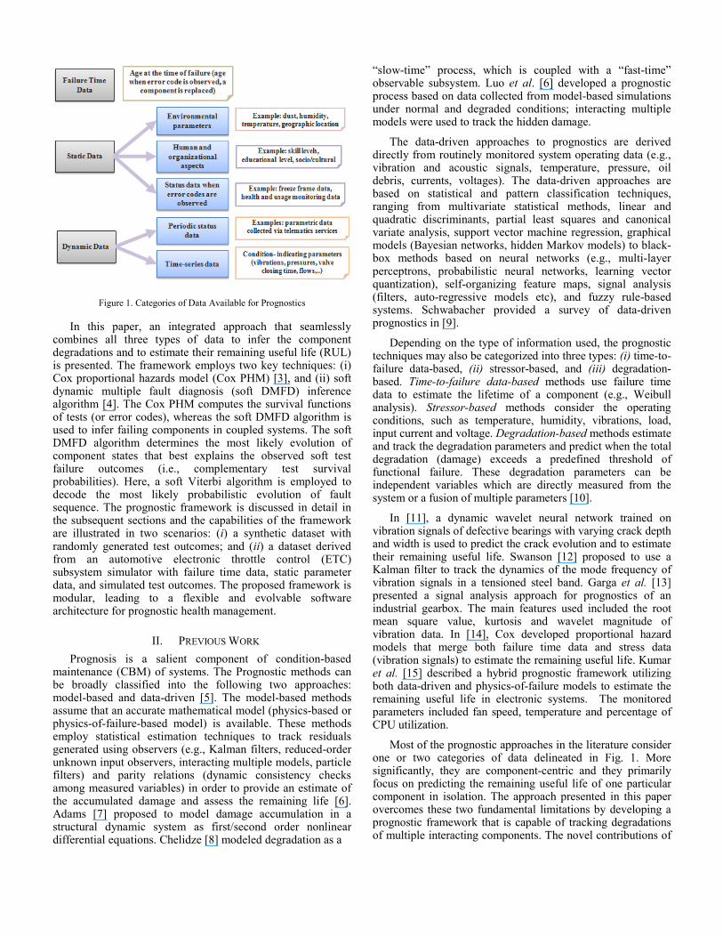
Figure 1. Categories of Data Available for Prognostics

In this paper, an integrated approach that seamlessly combines all three types of data to infer the component degradations and to estimate their remaining useful life (RUL) is presented. The framework employs two key techniques: (i) Cox proportional hazards model (Cox PHM) [3], and (ii) soft dynamic multiple fault diagnosis (soft DMFD) inference algorithm [4]. The Cox PHM computes the survival functions of tests (or error codes), whereas the soft DMFD algorithm is used to infer failing components in coupled systems. The soft DMFD algorithm determines the most likely evolution of component states that best explains the observed soft test failure outcomes (i.e., complementary test survival probabilities). Here, a soft Viterbi algorithm is employed to decode the most likely probabilistic evolution of fault sequence. The prognostic framework is discussed in detail in the subsequent sections and the capabilities of the framework are illustrated in two scenarios: (i) a synthetic dataset with randomly generated test outcomes; and (ii) a dataset derived from an automotive electronic throttle control (ETC) subsystem simulator with failure time data, static parameter data, and simulated test outcomes. The proposed framework is modular, leading to a flexible and evolvable software architecture for prognostic health management.

II. PREVIOUS WORK Prognosis is a salient component of condition-based

maintenance (CBM) of systems. The Prognostic methods can be broadly classified into the following two approaches: model-based and data-driven [5]. The model-based methods assume that an accurate mathematical model (physics-based or physics-of-failure-based model) is available. These methods employ statistical estimation techniques to track residuals generated using observers (e.g., Kalman filters, reduced-order unknown input observers, interacting multiple models, particle filters) and parity relations (dynamic consistency checks among measured variables) in order to provide an estimate of the accumulated damage and assess the remaining life [6]. Adams [7] proposed to model damage accumulation in a structural dynamic system as first/second order nonlinear differential equations. Chelidze [8] modeled degradation as a

“slow-time” process, which is coupled with a “fast-time” observable subsystem. Luo et al. [6] developed a prognostic process based on data collected from model-based simulations under normal and degraded conditions; interacting multiple models were used to track the hidden damage.

The data-driven approaches to prognostics are derived directly from routinely monitored system operating data (e.g., vibration and acoustic signals, temperature, pressure, oil debris, currents, voltages). The data-driven approaches are based on statistical and pattern classification techniques, ranging from multivariate statistical methods, linear and quadratic discriminants, partial least squares and canonical variate analysis, support vector machine regression, graphical models (Bayesian networks, hidden Markov models) to black-box methods based on neural networks (e.g., multi-layer perceptrons, probabilistic neural networks, learning vector quantization), self-organizing feature maps, signal analysis (filters, auto-regressive models etc), and fuzzy rule-based systems. Schwabacher provided a survey of data-driven prognostics in [9].

Depending on the type of information used, the prognostic techniques may also be categorized into three types: (i) time-to-failure data-based, (ii) stressor-based, and (iii) degradation-based. Time-to-failure data-based methods use failure time data to estimate the lifetime of a component (e.g., Weibull analysis). Stressor-based methods consider the operating conditions, such as temperature, humidity, vibrations, load, input current and voltage. Degradation-based methods estimate and track the degradation parameters and predict when the total degradation (damage) exceeds a predefined threshold of functional failure. These degradation parameters can be independent variables which are directly measured from the system or a fusion of multiple parameters [10].

In [11], a dynamic wavelet neural network trained on vibration signals of defective bearings with varying crack depth and width is used to predict the crack evolution and to estimate their remaining useful life. Swanson [12] proposed to use a Kalman filter to track the dynamics of the mode frequency of vibration signals in a tensioned steel band. Garga et al. [13] presented a signal analysis approach for prognostics of an industrial gearbox. The main features used included the root mean square value, kurtosis and wavelet magnitude of vibration data. In [14], Cox developed proportional hazard models that merge both failure time data and stress data (vibration signals) to estimate the remaining useful life. Kumar et al. [15] described a hybrid prognostic framework utilizing both data-driven and physics-of-failure models to estimate the remaining useful life in electronic systems. The monitored parameters included fan speed, temperature and percentage of CPU utilization.

Most of the prognostic approaches in the literature consider one or two categories of data delineated in Fig. 1. More significantly, they are component-centric and they primarily focus on predicting the remaining useful life of one particular component in isolation. The approach presented in this paper overcomes these two fundamental limitations by developing a prognostic framework that is capable of tracking degradations of multiple interacting components. The novel contributions of

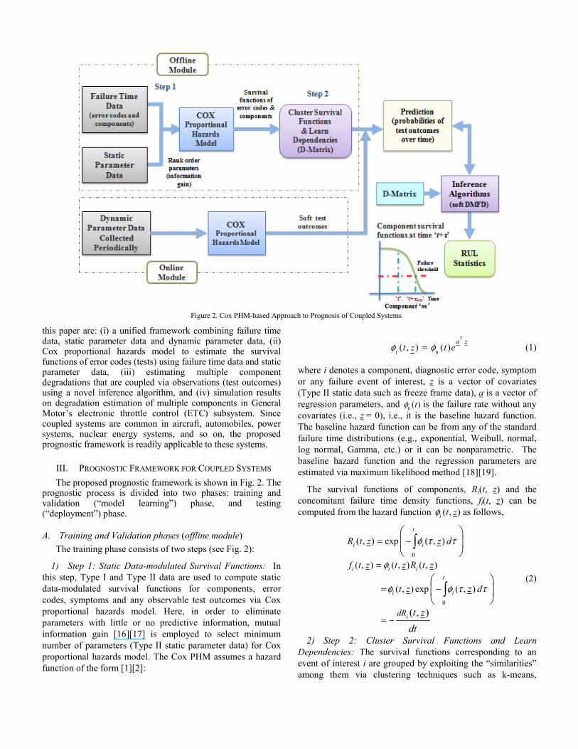
Figure 2. Cox PHM-based Approach to Prognosis of Coupled Systems

this paper are: (i) a unified framework combining failure time data, static parameter data and dynamic parameter data, (ii) Cox proportional hazards model to estimate the survival functions of error codes (tests) using failure time data and static parameter data, (iii) estimating multiple component degradations that are coupled via observations (test outcomes) using a novel inference algorithm, and (iv) simulation results on degradation estimation of multiple components in General Motor’s electronic throttle control (ETC) subsystem. Since coupled systems are common in aircraft, automobiles, power systems, nuclear energy systems, and so on, the proposed prognostic framework is readily applicable to these systems.

III. PROGNOSTIC FRAMEWORK FOR COUPLED SYSTEMS The proposed prognostic framework is shown in Fig. 2. The

prognostic process is divided into two phases: training and validation (“model learning”) phase, and testing (“deployment”) phase.

A. Training and Validation phases (offline module) The training phase consists of two steps (see Fig. 2):

1) Step 1: Static Data-modulated Survival Functions: In this step, Type I and Type II data are used to compute static data-modulated survival functions for components, error codes, symptoms and any observable test outcomes via Cox proportional hazards model. Here, in order to eliminate parameters with little or no predictive information, mutual information gain [16][17] is employed to select minimum number of parameters (Type II static parameter data) for Cox proportional hazards model. The Cox PHM assumes a hazard function of the form [1][2]:

0( , ) ( )

T

i

a zzt t eφ φ= (1)

where i denotes a component, diagnostic error code, symptom or any failure event of interest, z is a vector of covariates (Type II static data such as freeze frame data), a is a vector of regression parameters, and 0 ( )tφ is the failure rate without any covariates (i.e., z = 0), i.e., it is the baseline hazard function. The baseline hazard function can be from any of the standard failure time distributions (e.g., exponential, Weibull, normal, log normal, Gamma, etc.) or it can be nonparametric. The baseline hazard function and the regression parameters are estimated via maximum likelihood method [18][19].

The survival functions of components, Ri(t, z) and the concomitant failure time density functions, fi(t, z) can be computed from the hazard function ( , )i ztφ as follows,

0

0

( , ) exp ( , )

( , ) ( , ) ( , )

( , ) exp ( , )

( , )

t

i i

i i it

i i

idR

R t z z d

f t z t z R t z

t z dz

t zdt

φ τ τ

φ

φ φ τ τ

= −

=

= −

= −

⎛ ⎞⎜ ⎟⎝ ⎠

⎛ ⎞⎜ ⎟⎝ ⎠

∫

∫ (2)

2) Step 2: Cluster Survival Functions and Learn Dependencies: The survival functions corresponding to an event of interest i are grouped by exploiting the “similarities” among them via clustering techniques such as k-means,

learning vector quantization (LVQ), Gaussian mixture models (GMM), or hierarchical clustering [16][17]. The clustering process has the beneficial effects of revealing the usage patterns of system and the benefit of compressing the data for training. For coupled systems, probabilistic dependencies between the error codes and other observables (i.e., symptoms), and the component failure modes are estimated via maximum likelihood estimation procedure. These probabilistic dependencies are in the form of a matrix of likelihoods of observing an error code or other observables given a failure mode and is given by,

( , )ˆˆ ( | )( )

= ⇒ =ij j iij j i

i i

n n o FMp P o FM

n n FM (3)

where oj is the error code j, nij is the number of times oj is associated with failure mode i (FMi) and ni is the total number of observed cases with FMi. In order to avoid the problem with ML estimates, viz., the possibility of having a zero probability because of an unseen combination of (oj, FMi) in the training data, Laplacian smoothing [20] is used as follows:

( , ) 1ˆ( | )( ) | |

+=

+j i

j ii

n o FMP o FM

n FM FM (4)

where |FM| is the number of system failure modes.

The dependency matrix can be either binary (hard (0 or 1)) or probabilistic (soft). This dependency matrix captures the causal relationships between failure modes and error codes (or symptoms). In order to illustrate the process of developing the dependency matrix, let us consider an example shown in Table I. The example shows that there are three components (s1- s3); out of the six cases, component s1 failed thrice, component s2 failed twice, and component s3 failed only once. Each of these component failures resulted in a set of error codes, e.g., symptoms o1 and o3 are observed when component s2 failed. The failure modes are constructed by a combination of components and symptoms. In other words, if error codes o1 and o3 are observed then FM4 is the failure mode and s2 is the component to be replaced. Since error code o1 is present two-out-of-three times when s1 has failed, these occurrence counts among error codes and failure modes are used to derive the soft D-matrix, i.e., the matrix of likelihoods (see Table II). For example: FM1-o1 association weight 2/3 is derived by dividing the number of times oj is associated with s1. A purely binary (hard) D-matrix can also be derived which shows that if there

Table I. Sample Data of Observed Cases

Case No. Component Failed Failure Mode Error codes (Symptoms)

o1 o2 o3

1 s1 FM1 present absent absent 2 s1 FM1 present absent absent 3 s1 FM2 absent present absent 4 s2 FM3 Present Present absent 5 s2 FM4 Present Absent present 6 s3 FM5 Absent present present

Table II. Soft (Hard) D-Matrix

Failure Mode

Error codes (Symptoms)o1 o2 o3

FM1 2/3 (1) 0 (0) 0 (0) FM2 0 (0) 1/3 (1) 0 (0) FM3 1 (1) 1/2 (1) 0 (0) FM4 1 (1) 0(0) 1/2 (1) FM5 0 (0) 1(1) 1 (1)

is a 1 in the D-matrix, it implies that a specific failure mode can be detected by a specific error code (e.g., FM2 can be detected by o2). Refer to [21] for other methods of generating dependency matrices.

B. Testing (Deployment) Phase (online module) When new feature data y(t) (Type III dynamic data) is

obtained via online data acquisition systems, the survival probabilities of error codes (see (5)) are estimated using Cox PHM model as well as the baseline hazard functions obtained from the offline module (from Type I and Type II data).

0

0

( )

( , ( )) exp ( , ( ))

( , ( )) ( )T

j j

jt

ta yy

y yR t t d

t t t e

φ τ τ τ

φ φ

=

=

⇒ −⎛ ⎞⎜ ⎟⎝ ⎠∫ (5)

Here j refers to error codes (tests, symptoms). These soft error code outcomes are used to infer the failing components via the soft DMFD based on the D-matrix. The soft DMFD determines the evolution of fault states (complementary survival functions) given the soft error code outcomes at the observed time t. A detailed explanation of the algorithm is given in Section IV.

Once the component survival functions are obtained, the first and second order moments of time-to-failure T can be computed from the survival functions R(t) via (6) and (7), respectively [22].

0

( ) ( )τ τ∞

= ∫E T R d (6)

0 0

2

( ) 2 ( ) ( )Var T R d R dτ τ τ τ τ∞ ∞

=⎛ ⎞ ⎡ ⎤

−⎜ ⎟ ⎢ ⎥⎝ ⎠ ⎣ ⎦∫ ∫ (7)

Alternately, the remaining useful life (RUL) of a component at any time t can be computed from the survival function by defining a threshold on the survival probability.

Mathematically, it is written as,

( )0

( ) ( )arg minRUL t R tτ

τ ε= + ≤ (8)

where ε0 denotes the threshold of functional failure.

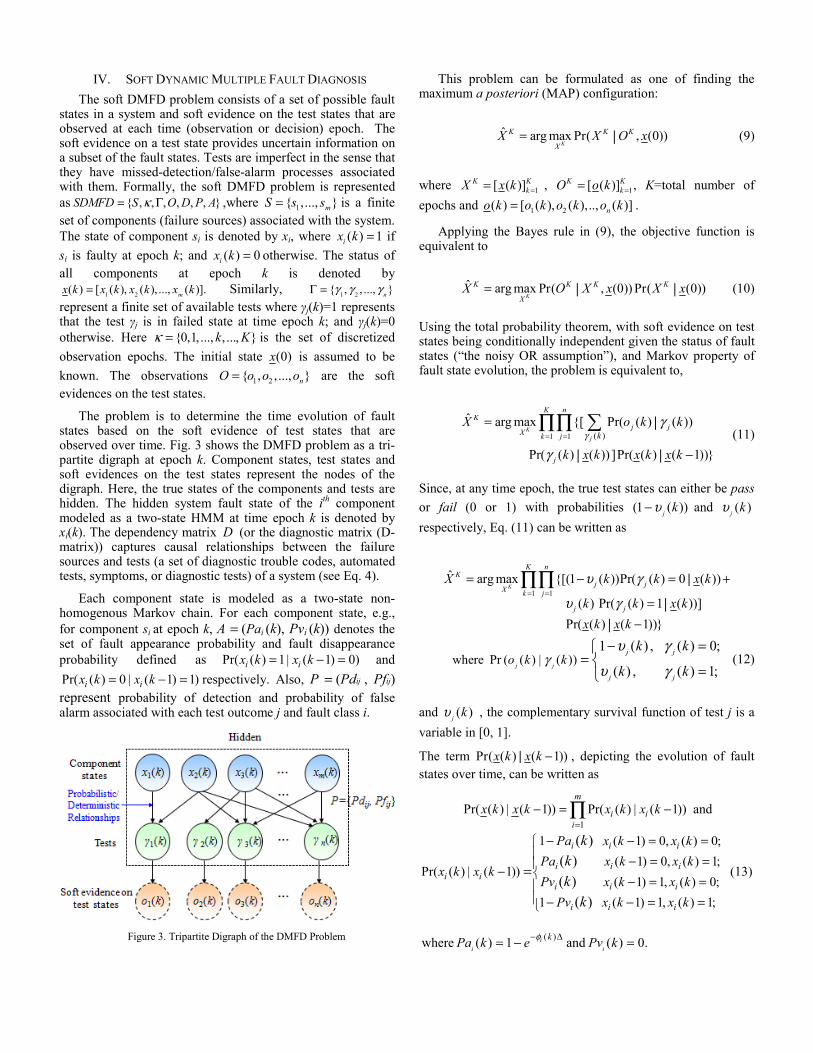
IV. SOFT DYNAMIC MULTIPLE FAULT DIAGNOSIS The soft DMFD problem consists of a set of possible fault

states in a system and soft evidence on the test states that are observed at each time (observation or decision) epoch. The soft evidence on a test state provides uncertain information on a subset of the fault states. Tests are imperfect in the sense that they have missed-detection/false-alarm processes associated with them. Formally, the soft DMFD problem is represented as { , , , , , , }SDMFD S O D P Aκ= Γ ,where 1{ }mS s s= ,..., is a finite set of components (failure sources) associated with the system. The state of component si is denoted by xi, where ( ) 1ix k = if si is faulty at epoch k; and ( ) 0ix k = otherwise. The status of all components at epoch k is denoted by

1 2( ) [ ( ) ( ) ( )].mx k x k x k x k= , , ..., Similarly, 1 2{ }nγ γ γΓ = , , ..., represent a finite set of available tests where γj(k)=1 represents that the test γj is in failed state at time epoch k; and γj(k)=0 otherwise. Here {0 1, , }κ = , ..., , ...k K is the set of discretized observation epochs. The initial state (0)x is assumed to be known. The observations 1 2{ }= , ,..., nO o o o are the soft evidences on the test states.

The problem is to determine the time evolution of fault states based on the soft evidence of test states that are observed over time. Fig. 3 shows the DMFD problem as a tri-partite digraph at epoch k. Component states, test states and soft evidences on the test states represent the nodes of the digraph. Here, the true states of the components and tests are hidden. The hidden system fault state of the ith component modeled as a two-state HMM at time epoch k is denoted by xi(k). The dependency matrix D (or the diagnostic matrix (D-matrix)) captures causal relationships between the failure sources and tests (a set of diagnostic trouble codes, automated tests, symptoms, or diagnostic tests) of a system (see Eq. 4).

Each component state is modeled as a two-state non-homogenous Markov chain. For each component state, e.g., for component si at epoch k, A = (Pai (k), Pvi (k)) denotes the set of fault appearance probability and fault disappearance probability defined as Pr( ( ) 1 | ( 1) 0)= − =i ix k x k and Pr( ( ) 0 | ( 1) 1)= − =i ix k x k respectively. Also, P = (Pdij , Pfij) represent probability of detection and probability of false alarm associated with each test outcome j and fault class i.

Figure 3. Tripartite Digraph of the DMFD Problem

This problem can be formulated as one of finding the maximum a posteriori (MAP) configuration:

ˆ arg max Pr( (0))= | ,K

K K K

XX X O x (9)

where 1[ ( )] ==K KkX x k , 1[ ( )] ,==K K

kO o k K=total number of epochs and 1 2( ) [ ( ), ( ),.., ( )]= no k o k o k o k .

Applying the Bayes rule in (9), the objective function is equivalent to

ˆ arg max Pr( (0)) Pr( (0))= | , |K

K K K K

XX O X x X x (10)

Using the total probability theorem, with soft evidence on test states being conditionally independent given the status of fault states (“the noisy OR assumption”), and Markov property of fault state evolution, the problem is equivalent to,

1 1 ( )

ˆ arg max {[ Pr( ( ) ( ))

Pr( ( ) ( )) ]Pr( ( ) ( 1))}

K

j

K nK

j jX k j

j

kX o k k

k x k x k x kγ

γ

γ= =

= |

| | −

∑∏∏ (11)

Since, at any time epoch, the true test states can either be pass or fail (0 or 1) with probabilities (1 ( ))j kυ− and ( )j kυ respectively, Eq. (11) can be written as

1 1

ˆ arg max {[(1 ( ))Pr( ( ) 0 ( ))

( ) Pr( ( ) 1 ( ))]Pr( ( ) ( 1))}

K

K nK

j jX k j

j j

X k k x k

k k x kx k x k

υ γ

υ γ= =

= − = | +

= || −

∏∏

where Pr ( ( ) | ( ))1 ( ) , ( ) 0;

( ) , ( ) 1;j j

j j

j j

o k kk k

k kγ

υ γ

υ γ

− ==

=

⎧⎨⎩

(12)

and ( )j kυ , the complementary survival function of test j is a variable in [0, 1].

The term Pr( ( ) ( 1))x k x k| − , depicting the evolution of fault states over time, can be written as

1Pr( ( ) | ( 1)) Pr( ( ) | ( 1))

m

i ii

x k x k x k x k=

− = −∏ and

1 ( 1) 0, ( ) 0;( 1) 0, ( ) 1;

Pr( ( ) | ( 1))( 1) 1, ( ) 0;

1 ( 1) 1, ( ) 1;

( )( )( )

( )

i i i

i i ii i

i i i

i i i

Pa x k x kPa x k x k

x k x kPv x k x k

Pv x k x k

kkk

k

− − = =⎧⎪ − = =⎪− ⎨ − = =⎪⎪ − − = =⎩

= (13)

( )where ( ) 1 and ( ) 0.i i

i kPa k e Pv kφ− Δ= − =

Here ( )i kφ denotes the failure rate of component i and Δ denotes the time step (for e.g., weeks, days, etc). It is assumed that the disappearance probability of a component i is zero i.e., if a component xi has failed at k-1, it remains in that state at time instant k. In other words, state ‘0’ is an absorbing state.

Following the procedure in [23], the primal function for the problem in (9) can be obtained as,

1

1 1

1

( ( ), ( 1), ( ))

ln{(1 ( )) ( )+ ( )(1 ( ))}

( ) ( ) ( ) ( 1)

( ) ( ) ( 1) ( )

kn

j j j jj

m m

i i i ii i

m

i i ii

f x k x k y k

k y k k y k

k x k k x k

h k x k x k g k

υ υ

μ σ=

= =

=

− =

− − +

− − +

− +

∑

∑ ∑

∑

( )( ) ln ; ( ) ln(1 ( ));1 ( )

where, ii i i

i

Pa kk k Pa kPa k

μ σ⎛ ⎞

= = −⎜ ⎟−⎝ ⎠

1

( ) ( ); ( ) ln(1 ( ))m

i i ii

h k k g k Pa kμ=

= − = −∑

1

1

( ) (1 ( ))( ) [(1 ) (1 ) ]

ln ( ) ( )

i im

j ij iji

m

j i ij ji

x k x ky k Pd Pf

y k x k c η=

=

−= − −

⇒ = +

∏∑

1

1where ln ln(1 )

1, j

i

mij

ij ijij

Pdc Pf

Pfη

=

−= = −

−

⎛ ⎞⎜ ⎟⎝ ⎠

∑ (14)

Exploiting the concavity of the log function in Eq. (14) and using Jensen’s inequality [17], a lower bound on the primal function can be written as1,

1

1 1

1

( ( ), ( 1), ( ))

{(1 ( )) ln ( )+ ( ) ln(1 ( ))}

( ) ( ) ( ) ( 1)

( ) ( ) ( 1) ( )

kn

j j j jj

m m

i i i ii i

m

i i ii

f x k x k y k

k y k k y k

k x k k x k

h k x k x k g k

υ υ

μ σ=

= =

=

− ≤

− − +

− − +

− +

∑

∑ ∑

∑

(15)

The optimal * ( )jy k obtained by optimizing the Lagrangian function as in [23] is,

( )( )

( ) ( )λ

λ υ=

+j

jj j

ky k

k k (16)

1 This approximation enables us to use the DMFD algorithm in [23] with minor modifications and the exact version will be pursued elsewhere.

where ={ ( ) 0, (1, ), (1, )}j k k K j nλΛ ≥ ∈ ∈ is the set of Lagrange multipliers.

The dual function can be written as [23],

1

( , ) max ( )=

Λ = Λ∑K

m

iX i

Q X Q

1

where ( )1( ( ), ( 1), ( )) ( )i

K

i i i j kk

Q x k x k k wm

ξ λ=

Λ = − + Λ∑ (17)

[(1 ( )) ( ) ] ( )

( ) ( 1) ( ) ( ) ( 1)( )

( ), ( 1), ( )( )

{ }j ij j ij i

i

i i i i i

ij

i i j

k c k c k

k x k h k x k x kx k

x k x k k

υ λ μ

ξ

σ

λ

− − +

=

− + −

−

− +∑

1 ( )

ln ( ) ( )

( )[ln ( ) ln( ( ) ( ))]

( ) ( ) ( )

( )[ ( ) ln( )]

[ ]

j j

j j

jj

j

j jj

k j j

j j

k

k k

k k k k

w g k k

k k

υ λ

υ υ υ λ

λ λ υ λ

η−

+

+ − +

Λ = + − +

−

∑∑∑

(18)

As in Eq. (17), the Lagrangian relaxation algorithm decomposes the original soft DMFD problem into m separable subproblems. The Lagrange multipliers are updated iteratively using the subgradient method; and Viterbi algorithm is used to find the most likely fault sequence [23]. At each epoch, a Sigmoid function is employed to relax the fault states to have values in the real interval [0,1], a soft decision variable; it is interpreted as a pseudo marginal posterior probability. The soft fault states (complementary survival probabilities (1-Ri(k))) are given by [4]:

1( ) , ( ) [0,1],

1 exp( (0, 0) (1,1))for 1, ..., .

is

ii i

x k x k

i mξ ξ

= =+ −

= (19)

V. EXPERIMENTAL RESULTS The prognostic framework is applied to two different

scenarios. (A) Scenario 1: a synthetic dataset with randomly generated test outcomes, and (B) Scenario 2: dataset derived from an automotive electronic throttle control (ETC) subsystem simulator with failure time data, static parameter data and simulated test outcomes. The experimental results are briefly discussed in the following subsections.

A. Scenario 1 In this scenario, the prognostic framework is applied to a

small synthetic dataset with a 5x5 D-matrix shown in Table III [24]. Here, each test covers two or more faults, for example, γ1 detects faults in either or both of s3 and s4, i.e., the component states are coupled via observations (test outcomes). Initially, the complementary component survival functions (component degradations) are assumed to be of sigmoid (S-) shape with

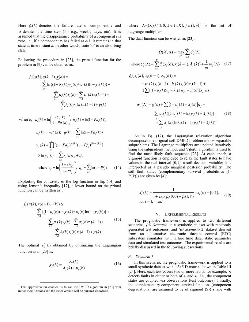
degradation/failure probabilities varying between 0 and 1. The degradation curves for components (s1-s5) are as shown in Fig. 4. At any epoch k, the test outcomes are generated from the component state survival probabilities via the noisy-OR model (e.g., [23][25])

1

Pr( ( ) 1| ( )) ( ) 1

{ ( )(1 ) (1 ( ))(1 )}

j j

m

i ij i iji

k x k k

R k Pf R k Pd

γ υ

=

= = = −

− + − −∏ (20)

where Ri(k) is the survival probability of component i at time epoch k, (Pdij,Pfij) are the detection and false alarm probabilities associated with each component and test. These probabilistic test outcomes are then fed to the soft DMFD algorithm to infer the component degradations at any time epoch k. Under a single fault assumption, Fig. 5 shows the estimated component probability when s2 is faulty and Fig. 6 shows the estimated component probability when s5 is faulty. In Fig. 6, although component s5 is degrading with time, the algorithm infers s2, s4 and s5 as failing components since faults s2 and s4 are hidden faults of s5 (see Table III). The estimated component failure probability is close to the true failure component probability with R-square fit of about 99% for all the components. This is an ideal scenario with perfect test outcomes (i.e., tests have high detection probability and low false alarm probability). However, the real data is unlikely to produce this type of accuracies.

Table III. Diagnostic (D-) Matrix for Scenario 1

γ1 γ2 γ3 γ4 γ5

s1 0 1 0 0 1

s2 0 0 1 1 0

s3 1 0 0 1 1

s4 1 1 0 0 0

s5 1 1 1 1 0

0 200 400 600 800 1000 1200 1400 16000

0.1

0.2

0.3

0.4

0.5

0.6

0.7

0.8

0.9

1Failure Probability (Degradation) Curves for Components

Age (in days)

Fai

lure

Pro

babi

lity

s1

s2

s3s4

s5

Figure 4. Component Degradation Curves

0 200 400 600 800 1000 1200 1400 16000

0.1

0.2

0.3

0.4

0.5

0.6

0.7

0.8

0.9

1Failure Probability (Degradation) curve for s2

Age (in days)

Fai

lure

Pro

babi

lity

Estimated s1Estimated s2

Estimated s3

Estimated s4

Estimated s5True s2

R-square = 99.45MSE = 0.0008

Figure 5. Estimated Degradation Curve for Component s2

0 200 400 600 800 1000 1200 1400 16000

0.1

0.2

0.3

0.4

0.5

0.6

0.7

0.8

0.9

1Failure Probability (Degradation) Curve for s5

Age (in days)

Fai

lure

Pro

babi

lity

Estimated s1Estimated s2

Estimated s3

Estimated s4

Estimated s5True s5

R-square = 99.22MSE = 0.0015

Figure 6. Estimated Degradation Curve for Component s5

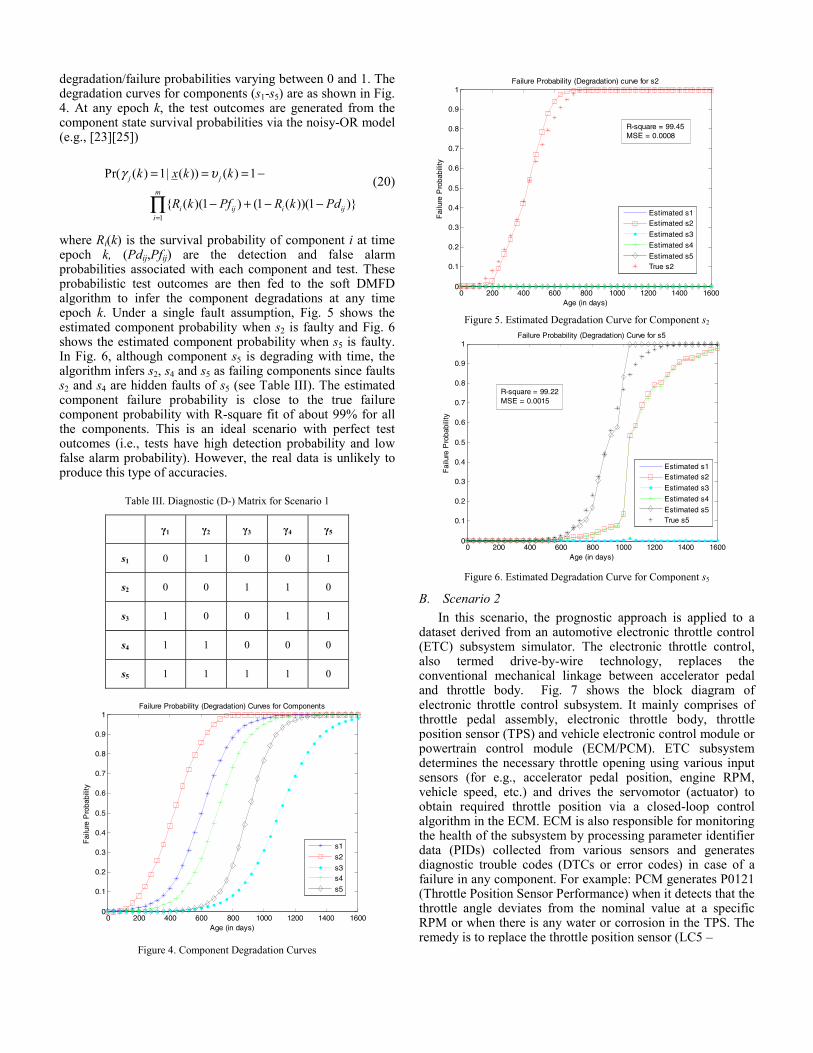
B. Scenario 2 In this scenario, the prognostic approach is applied to a

dataset derived from an automotive electronic throttle control (ETC) subsystem simulator. The electronic throttle control, also termed drive-by-wire technology, replaces the conventional mechanical linkage between accelerator pedal and throttle body. Fig. 7 shows the block diagram of electronic throttle control subsystem. It mainly comprises of throttle pedal assembly, electronic throttle body, throttle position sensor (TPS) and vehicle electronic control module or powertrain control module (ECM/PCM). ETC subsystem determines the necessary throttle opening using various input sensors (for e.g., accelerator pedal position, engine RPM, vehicle speed, etc.) and drives the servomotor (actuator) to obtain required throttle position via a closed-loop control algorithm in the ECM. ECM is also responsible for monitoring the health of the subsystem by processing parameter identifier data (PIDs) collected from various sensors and generates diagnostic trouble codes (DTCs or error codes) in case of a failure in any component. For example: PCM generates P0121 (Throttle Position Sensor Performance) when it detects that the throttle angle deviates from the nominal value at a specific RPM or when there is any water or corrosion in the TPS. The remedy is to replace the throttle position sensor (LC5 –

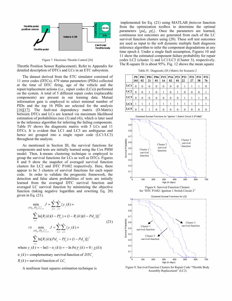
Figure 7. Electronic Throttle Control [26]

Throttle Position Sensor Replacement). Refer to Appendix for detailed description of DTCs and LCs in an ETC subsystem.

The dataset derived from the ETC simulator consisted of 11 error codes (DTCs), 479 status parameters (PIDs) collected at the time of DTC firing, age of the vehicle and the repair/replacement actions (i.e., repair codes (LCs)) performed on the system. A total of 5 different repair codes (replaceable components) are present in our training data. Mutual information gain is employed to select minimal number of PIDs and the top 16 PIDs are selected for the analysis [16][17]. The fault-test dependency matrix (D-Matrix) between DTCs and LCs are learned via maximum likelihood estimation of probabilities (see (3) and (4)), which is later used in the inference algorithm for inferring the failing components. Table IV shows the diagnostic matrix with 5 LCs and 11 DTCs. It is evident that LC1 and LC3 are ambiguous and hence are grouped into a single repair code (LC1/LC3) throughout the analysis.

As mentioned in Section III, the survival functions for components and tests are initially learned using the Cox PHM model. Then, k-means clustering technique is employed to group the survival functions for LCs as well as DTCs. Figures 8 and 9 show the snapshot of averaged survival function clusters for LC2 and DTC P1682 respectively. Here, there appear to be 3 clusters of survival functions for each repair code. In order to validate the prognostic framework, the detection and false alarm probabilities of tests are initially learned from the averaged DTC survival function and averaged LC survival function by minimizing the objective function (taking negative logarithm and rewriting Eq. 20) given in Eq. (21).

,1, 1

,1, 1

1 1

2

1

1 1

2

1

{ }

{ }

,

,

min { ( )

ln[ ( )(1 ) (1 ( ))(1 )]}

min { ( )

ln[ ( )( ) (1 )]}

m ni j

m ni j

K n

jij ij k j

m

i ij i iji

K n

jij ij k j

m

i ij ij iji

Pd

Pd

Pf

Pf

J y k

R k Pf R k Pd

J y k

R k Pd Pf Pd

= =

= =

= =

=

= =

=

= +

− + − −

= +

− + −

⇒

∑∑

∑

∑∑

∑

(21)

Pr( )where ( ) ln(1 ( )) ln ( ) 0 | ( )j j jy k k k x kυ γ= − − = − =

( ) complementary survival function of( ) survival function of

j j

i i

k DTCR k LCυ =

=

A nonlinear least squares estimation technique is

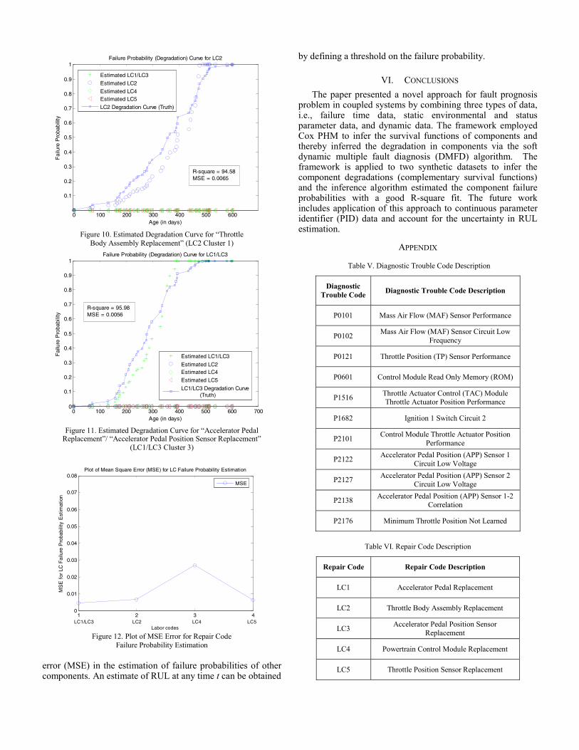
implemented for Eq. (21) using MATLAB fmincon function from the optimization toolbox to determine the optimal parameters {pdij, pfij}. Once the parameters are learned, continuous test outcomes are generated from each of the LC survival function clusters using (20). These soft test outcomes are used as input to the soft dynamic multiple fault diagnosis inference algorithm to infer the component degradations at any time epoch k. Under a single fault assumption, Figures 10 and 11 show the estimated component failure probability for repair codes LC2 (cluster 1) and LC1/LC3 (Cluster 3), respectively. The R-square fit is about 95%. Fig. 12 shows the mean square

Table IV. Diagnostic (D-) Matrix for Scenario 2

P0101

P0102

P0121

P0601

P1516

P1682

P2101

P2122

P2127

P2138

P2176

LC1 0 0 0 0 0 0 0 1 1 1 0

LC2 0 0 1 0 1 0 1 0 0 0 1

LC3 0 0 0 0 0 0 0 1 1 1 0

LC4 1 1 1 1 1 1 1 1 1 1 1

LC5 0 0 1 0 0 0 0 0 0 0 0

0 100 200 300 400 500 600 7000

0.1

0.2

0.3

0.4

0.5

0.6

0.7

0.8

0.9

1

Age (in days)

Sur

viva

l Pro

babi

lity

Clustered Survival Functions for "Ignition 1 Switch Circuit 2 (P1682)"

Figure 8. Survival Function Clusters

for “DTC P1682- Ignition 1 Switch Circuit 2”

0 100 200 300 400 500 600 7000

0.1

0.2

0.3

0.4

0.5

0.6

0.7

0.8

0.9

1

Age (in days)

Sur

viva

l Pro

babi

lity

Clustered Survival Functions for LC2

Figure 9. Survival Function Clusters for Repair Code “Throttle Body

Assembly Replacement” (LC2)

Cluster 1 survival function

Cluster 2 survival function

Cluster 3 survival function

Cluster 1 survival function

Cluster 2 survival function

Cluster 3 survival function

0 100 200 300 400 500 600

0.1

0.2

0.3

0.4

0.5

0.6

0.7

0.8

0.9

1

Age (in days)

Fai

lure

Pro

babi

lity

Failure Probability (Degradation) Curve for LC2

Estimated LC1/LC3

Estimated LC2

Estimated LC4Estimated LC5

LC2 Degradation Curve (Truth)

R-square = 94.58MSE = 0.0065

Figure 10. Estimated Degradation Curve for “Throttle

Body Assembly Replacement” (LC2 Cluster 1)

0 100 200 300 400 500 600 7000

0.1

0.2

0.3

0.4

0.5

0.6

0.7

0.8

0.9

1

Age (in days)

Fai

lure

Pro

babi

lity

Failure Probability (Degradation) Curve for LC1/LC3

Estimated LC1/LC3

Estimated LC2Estimated LC4

Estimated LC5

LC1/LC3 Degradation Curve (Truth)

R-square = 95.98MSE = 0.0056

Figure 11. Estimated Degradation Curve for “Accelerator Pedal

Replacement”/ “Accelerator Pedal Position Sensor Replacement” (LC1/LC3 Cluster 3)

1 2 3 40

0.01

0.02

0.03

0.04

0.05

0.06

0.07

0.08

LC1/LC3 LC2 LC4 LC5Labor codes

MS

E f

or L

C F

ailu

re P

roba

bilit

y E

stim

atio

n

Plot of Mean Square Error (MSE) for LC Failure Probability Estimation

MSE

Figure 12. Plot of MSE Error for Repair Code

Failure Probability Estimation

error (MSE) in the estimation of failure probabilities of other components. An estimate of RUL at any time t can be obtained

by defining a threshold on the failure probability.

VI. CONCLUSIONS The paper presented a novel approach for fault prognosis

problem in coupled systems by combining three types of data, i.e., failure time data, static environmental and status parameter data, and dynamic data. The framework employed Cox PHM to infer the survival functions of components and thereby inferred the degradation in components via the soft dynamic multiple fault diagnosis (DMFD) algorithm. The framework is applied to two synthetic datasets to infer the component degradations (complementary survival functions) and the inference algorithm estimated the component failure probabilities with a good R-square fit. The future work includes application of this approach to continuous parameter identifier (PID) data and account for the uncertainty in RUL estimation.

APPENDIX

Table V. Diagnostic Trouble Code Description

Diagnostic Trouble Code Diagnostic Trouble Code Description

P0101 Mass Air Flow (MAF) Sensor Performance

P0102 Mass Air Flow (MAF) Sensor Circuit Low Frequency

P0121 Throttle Position (TP) Sensor Performance

P0601 Control Module Read Only Memory (ROM)

P1516 Throttle Actuator Control (TAC) Module Throttle Actuator Position Performance

P1682 Ignition 1 Switch Circuit 2

P2101 Control Module Throttle Actuator Position Performance

P2122 Accelerator Pedal Position (APP) Sensor 1 Circuit Low Voltage

P2127 Accelerator Pedal Position (APP) Sensor 2 Circuit Low Voltage

P2138 Accelerator Pedal Position (APP) Sensor 1-2 Correlation

P2176 Minimum Throttle Position Not Learned

Table VI. Repair Code Description

Repair Code Repair Code Description

LC1 Accelerator Pedal Replacement

LC2 Throttle Body Assembly Replacement

LC3 Accelerator Pedal Position Sensor Replacement

LC4 Powertrain Control Module Replacement

LC5 Throttle Position Sensor Replacement

ACKNOWLEDGMENTS We thank GM ISL and NSF for their support of this work.

Any opinions expressed in this paper are solely those of the authors and do not represent those of the sponsors.

REFERENCES [1] A. K. S. Jardine and A. H. C. Tsang, Maintenance, Replacement, and Reliability: Theory and Applications, New York: CRC Press, 2005. [2] D. N. P. Murthy, M. Xie and R. Jiang, Weibull Models, New York: Wiley, 2004. [3] J. D. Klabfleisch and R. L. Prentice, “The Statistical Analysis of Failure Time Data,” 2nd edition, New York, Wiley, 2002. [4] S. Singh, A. Kodali, and K. Pattipati, “A factorial hidden Markov model-based reasoner for diagnosing multiple intermittent faults,” IEEE CASE, Bangalore, August 2009. [5] L. H. Chiang, E. Russel, and R. Braatz, “Fault detection and diagnosis in industrial systems”, London: Springer-Verlag, 2001. [6] J. Luo, M. Namburu, K. Pattipati, L. Qiao, M. Kawamoto, and S. Chigusa, “Model-based prognostic techniques”, IEEE Autotestcon Conference, 2003, pp. 330-340. [7] D. E. Adams, “Nonlinear damage models for diagnosis and prognosis in structural dynamic systems”, in SPIE Conference Proceedings, vol. 4733, 2002, pp. 1-12. [8] D. Chelidze, J. P. Cusumano, and A. Chatterjee, “ Dynamical systems approach to damage evolution tracking, part I: The experimental method”, Journal of Vibration and Acoustics, vol. 124, pp. 250-257, 2002. [9] M. A. Schwabacher, “ A survey of data-driven prognostics”, Infotech@Aerospace, American Institute of Aeronautics and Astronautics 2005-7002, Arlington, Virginia, September, 2005. [10] J. B. Coble, “Merging data sources to predict remaining useful life – an automated method to identify prognostic parameters”, PhD dissertation, University of Tennessee, 2010. [11] P. Wang and G. Vachtsevanos, “ Fault prognosis using dynamic wavelet neural networks”, in Maintenance and Reliability Conference (MARCON 99), May 1999. [12] D. Swanson, “ A general prognostic tracking algorithm for predictive maintenance”, in Proc. IEEE International Conference on Aerospace, vol.6, 2001, pp. 2971-2977. [13] A. K. Garga, K. T. Mcclintic, R. L. Campbell, C. C. Yang, and M. S. Lebold, “Hybrid reasoning for prognostic learning in cbm systems”, in IEEE, 2000, pp. 2957-2969. [14] D. R. Cox and D. Oakes, “Analysis of survival data”, Chapman and Hall,1984. [15] S. Kumar, M. Torres, Y. C. Chan, and M. Pecht, “A hybrid prognostics methodology for electronic products”, IEEE International Joint Conference on Neural Networks, 2008. [16] R.O. Duda, P.E. Hart and D. Stork, “Pattern classification”, John Wiley & Sons, New York, 2000. [17] C. M. Bishop, “Neural Networks for Pattern Recognition”, Clarendon Press, Oxford, 1997. [18] P. J. Vlok, J. L. Coetzee, D. Banjevic, A. K. S. Jardine and V. Makis, “Optimal Component Replacement Decisions Using Vibration Monitoring and the PHM,” Journal of the Operational Research Society, Vol. 53, 193-202, 2002. [19] J. P. Klein and M. L. Moeschberger, “ Survival Analysis Techniques for Censored and Truncated Data”, Springer-Verlag, New York, 2003. [20] D. Metzler, V. Lavrenko and W. B. Croft, “Formal Multiple Bernoulli Models for Language Modeling,” in. Proc. 27th Annual International ACM Conference on Research and Development in Information Retrieval (SIGIR’ 04), Sheffield, UK, 2004, pp. 540-541. [21] S. Singh, S. W. Holland, and P. Bandyopadhyay, “Trends in the development of system-level fault dependency models”, IEEE Aerospace Conference, March 2010. [22] Z. Ma and A. W. Krings, “Survival analysis approach to reliability, survivability and Prognostics and Health Management (PHM)”, IEEE Aerospace Conference, May 2008. [23] S. Singh, A. Kodali, K. Choi, K. Pattipati, S. M. Namburu, S. Chigusa, D. V. Prokhorov, and L. Qiao, “Dynamic Multiple Fault Diagnosis Problem

Formulations and Solution Techniques,” IEEE Trans. on Systems, Man and Cybernetics: Part A, vol. 39, no. 1, pp. 160-176, January 2009. [24] K. Pattipati and M. G. Alexandridis, “Application of heuristic search and information theory to sequential fault diagnosis”, IEEE International Symposium on Intelligent Control, pp. 291-296, August 1988. [25] J. Pearl, “Fusion, propagation and structuring in belief networks,” Artificial Intelligence, Vol. 29, No. 3, pp. 241-288, 1986. [26] http://www.picoauto.com/applications/electronic-throttle-control.html, accessed on November 14th, 2010.

BIOGRAPHY Chaitanya Sankavaram received the B.Tech. degree in Electrical and Electronics Engineering from Sri Venkateswara University, Tirupathi, India, in 2005. She is currently working toward the Ph.D. degree in Electrical and Computer Engineering at the University of Connecticut, Storrs. She was a Project Engineer with Wipro Technologies, Bangalore, India, for two years. Her current research interests include fault diagnosis and prognosis, reliability analysis, data mining, pattern recognition, and optimization theory.

Anuradha Kodali received the B.E. degree in Electronics and Communications Engineering from Andhra University, Visakhapatnam, India, in 2006. She is currently working toward the Ph.D. degree in Electrical and Computer Engineering at the University of Connecticut, Storrs. Her research interests include data mining, pattern recognition, fault detection and diagnosis, and optimization theory.

Krishna R. Pattipati (S’77---M’80---SM’91---F’95) received the B.Tech. degree in Electrical Engineering with highest honors from the Indian Institute of Technology, Kharagpur, India, in 1975 and the M.S. and Ph.D. degrees in Systems Engineering from the University of Connecticut, Storrs, in 1977 and 1980, respectively. From 1980 to 1986, he was with ALPHATECH, Inc., Burlington, MA. Since 1986, he has been with the University of Connecticut, where he is currently a Professor of Electrical and Computer Engineering and is selected as the UTC Chair Professor in Systems Engineering. He was a Consultant to Alphatech, Inc., Aptima, Inc., and IBM Research and Development. He is a Co-Founder of Qualtech Systems, Inc., which is a small business specializing in intelligent diagnostic software tools. His research interests include the areas of adaptive organizations for dynamic and uncertain environments, multiuser detection in wireless communications, signal processing and diagnosis techniques for complex system monitoring, and multi object tracking. He is a Fellow of IEEE.

Bing Wang received her B.S. degree in Computer Science from Nanjing University of Science & Technology, China in 1994, and M.S. degree in Computer Engineering from Institute of Computing Technology, Chinese Academy of Sciences in 1997. She then received M.S. degrees in Computer Science and Applied Mathematics, and a Ph.D. in Computer Science from the University of Massachusetts, Amherst in 2000, 2004, and 2005 respectively. She joined the Computer Science & Engineering Department at the University of Connecticut as an assistant professor in 2005. Her research interests are in computer networks, distributed systems and smart grid. She received NSF CAREER award in 2008.

Mohammad Azam received his MS in Electrical Engineering from University of Connecticut in 2002. Currently he is working as a Member, Technical Staff of the R&D and Professional Services at Qualtech Systems, Inc (QSI). At present, he is functioning as the technical lead for several of QSI’s research and development projects. His research interests include fault detection and isolation in complex engineering systems; fault and degradation forecasting in electronic, electrical and mechanical systems; self-healing control of navy machinery and spacecraft power systems; and optimal sensor allocation for fault detection and isolation.

Satnam Singh received his MS degree in Electrical Engineering from the University of Wyoming in 2003, and PhD degree in Electrical and Computer Engineering from the University of Connecticut in 2007. He is currently working as a Senior Researcher in the GM India Science Lab. He is a technical committee member of IEEE PHM Conference (Asia Region) since 2009 and served as a reviewer in several journals. He has published numerous journal and conference papers. His research interests include fault modeling, fault diagnosis and prognosis, graphical models, pattern recognition and data mining techniques.