RESEARCH PAPER

copy 2003 Blackwell Publishing Ltd httpwwwblackwellpublishingcomjournalsgeb

Global Ecology amp Biogeography

(2003)

12

103ndash118

Blackwell Science Ltd

A probabilistic approach to the use of pollen indicators for plant attributes and biomes an application to European vegetation at 0 and 6 ka

S GACHET S BREWERDagger R CHEDDADIDagger B DAVISDagger E GRITTIdaggersect and J GUIOTdagger

IMEP CNRS UMR 6116 Faculteacute de St-Jeacuterocircme case 461 F-13397 Marseille cedex 20 France E-mail sophiegachetunivu-3mrsfr

dagger

CEREGE CNRS UMR 6635 Europocircle Meacutediterraneacuteen de lrsquoArbois case 80 F-13545 Aix-en-Provence cedex 4 France E-mail guiotceregefr

Dagger

European Pollen Database Centre Universitaire drsquoArles 13200 Arles France and

sect

Department of Physical Geography and Ecosystems

Analysis Soumllvegatan 13 Lund University S-223 62 Lund Sweden

ABSTRACT

Aim

This paper presents a probabilistic method for thecharacterization of pollen taxa using attributes and for thereconstitution of past biomes The probabilities are calculatedon the basis of European floristic and pollen databasessufficiently large and exhaustive to provide robust estimates

Location

The analysis is based on data from approximately1000 sites throughout Europe

Method

We use all the pollen data from the European PollenDatabase (EPD) which contains about 50 000 pollen assem-blages distributed across Europe and covering the periodfrom the Last Glacial Maximum to the present Using existingfloras each pollen taxon has been characterized by allocatingone or more modes of several attributes chosen according tothe biogeography and phenology of the taxon With thisinformation conditional probabilities are defined represent-ing the chance of a given attribute mode occurring in a givenpollen spectrum when the taxa assemblage is known Theconcept of co-occurrence is used to provide a greater amount ofinformation to compensate for difficulties in the identification

of pollen grains allowing a better interpretation when there islittle diversity in the pollen assemblage

Results

The method has been validated using a dataset ofmodern samples against existing methods of biome classifica-tion and remote sensing data An application is proposed inwhich the new method is used to produce biomes for pollendata 6000 years ago This confirms previous results showingan extension of the deciduous forest to the north east andsouth explained by milder winters in western and northernEurope and cooler and wetter climate in the Mediterraneanregion

Conclusion

The results show the new method to be efficientreliable and flexible and to be an improvement over the pre-vious method of biomization They will be used to test simula-tions of earth system models running on periods with climatesignificantly different from the present day enabling a robusttest of the validity of applying these models to the future

Key words

biomes conditional probability Europe land-surface characteristics palaeovegetation reconstructionplant attributes pollen data

INTRODUCTION

The reliability of future climatic changes simulated byclimate models needs to be assessed as the ability of existingmodels to simulate the present climate varies considerably(McAvaney

et al

2001) When used to predict a climate verydifferent from the present one this variation may be expected

to increase This can be checked against reconstructions ofpast climates (Joussaume

et al

1999) providing an excellentmethod for the evaluation of model responses to climaticchanges The Palaeoclimate Modelling IntercomparisonProject (PMIP) (Joussaume amp Taylor 1995) has focused ontwo key periods the Last Glacial Maximum and the MiddleHolocene As an example this project has shown that most ofthe climate models simulate effectively the enhanced monsoonin Africa and Asia resulting from the increased seasonalityin insolation 6000 years ago (Joussaume

et al

1999) Thevalidation of such results requires palaeoclimatic data derived

Correspondence J Guiot CEREGE CNRS UMR 6635 EuropocircleMeacutediterraneacuteen de lrsquoArbois case 80 F-13545 Aix-en-Provence cedex4 France E-mail guiotceregefr

104

S Gachet

et al

copy 2003 Blackwell Publishing Ltd

Global Ecology amp Biogeography

12

103ndash118

from proxy data such as fossil pollen assemblages gatheredin large databases The pollen data can be calibrated in termsof climatic variables that may be comparable to the outputsof the climate models (Cheddadi 1997 Masson

et al

1999Pinot

et al

1999 Kageyama

et al

2001) Alternativelyvegetation models coupled to climate models can produceoutputs directly comparable to the pollen data (Texier

et al

1997 Harrison

et al

1998) Here the pollen data are used totest the combined performance of models of both types

In order to reduce the complexity and run time of globalvegetation models plant species are grouped together into alimited number of types by using functional classifications(Steffen

et al

1992) Concepts and definitions of functionaltypes differ between ecologists (Smith

et al

1996) Speciescan be grouped on the basis of the resources used (termedlsquoguildsrsquo) or by the response to a specific perturbation (termedlsquogroupsrsquo) Further subdivisions can be made species mayshare the same resource but use it in different ways alternat-ively they may respond to the same perturbation by differentmechanisms For example species that fall into the samebiogeographical unit have the same response to a givenclimate but not necessarily with the same mechanism Gitayamp Noble (1997) have described these as lsquoresponse groupsrsquo

The main goal of palaeoecology is the study of vegetationtemporal dynamics The reconstruction and interpretation ofthese dynamics is restricted by the type of data available forthe past In many cases pollen identification is not preciseenough to allow plant identification at species level due tothe state of preservation of fossil pollen grains or due tosimilar pollen morphology between species However this ispartly compensated for by the fact that the abundance of thedifferent types of plants is well quantified

The interpretation of pollen data is greatly aided bymultivariate methods (eg Prentice 1986 Grimm 1988Peng

et al

1994) and comprehensive sets of modern surfacesamples However the application of modern pollen samplesto the interpretation of past pollen spectra is limited by theexistence of vegetation assemblages that have no modernanalogues (Webb 1986) This limitation can be overcome bythe use of the large amount of data compiled in the EuropeanPollen Database (EPD) This database contains pollen spectrarepresentative of most of the European vegetation typesoccurring during the Quaternary period (including glacialtransitional and anthropogenic vegetation) and provides asolid basis for the approach developed here The quantity ofdata present in this database is sufficiently large to allow thedevelopment of a probabilistic method that is more flexiblethan the lsquobiomizationrsquo approach (Prentice

et al

1996)applied in the BIOME6000 project (Prentice

et al

2000) asprobabilities replace simple sums of percentages

The method of Prentice

et al

(1996) is a lsquofuzzy logicrsquoapproach in which a biome is assigned to each pollen samplein a series of steps

1

Plant functional types (PFT) are defined as groups oftaxa having the same response to a set of perturbations

2

For each pollen sample an estimate is made of thenumerical affinity with every biome To estimate this eachtaxon is initially assigned to a PFT on the basis of theknown biology of the species included

3

An affinity score is then calculated for each PFT as thesum of the pollen percentages of all the taxa included inthat type

4

A biome is then defined as a combination of PFT whollyor partly present in the biome and a biome score is calculatedfrom the sum of the corresponding PFT scores

5

Finally the pollen sample is assigned to the biome withwhich it has the greatest affinity

In our method we do not assign each taxon to one orseveral PFT but we assign all the attribute modes relevant toeach taxon on the basis of several floristic databases Thescores are replaced by probabilities which are dependent notonly on the pollen percentages but also on the frequencieswith which taxa co-occur in the EPD Afterwards a biome isdefined as a combination of attribute modes and on thisbasis a biome probability is calculated according to a set ofpredefined rules

Results have been obtained using Prenticersquos method for thedifferent continents of the globe (Jolly

et al

1998 Tarasov

et al

1998 Edwards

et al

2000 Elenga

et al

2000Tarasov

et al

2000 Thompson amp Anderson 2000 Williams

et al

2000)The method proposed in this paper exploits a characteristic

of the pollen data that has not been taken into account in theexisting biomization method although Tarasov

et al

(1998)used a similar approach to distinguish warm and cold steppebiomes The proposed approach uses the notion of the floristicassemblage (Ruffray

et al

1998) to compensate for thelack of acute identification of the pollen taxa This has beenused extensively in the ecological database SOPHY togetherwith the concept of a lsquoco-occurrencersquo probability that quanti-fies the probability of any two given taxa occurring in thesame site (Ruffray

et al

1998) The co-occurrence concept isused in this paper and is described further

DATA

The probablilities are calculated on 45928 samples fromapproximately 1000 sites throughout Europe covering thelast 21 ka In the following text this dataset is referred to aslsquothe EPD datasetrsquo It contains 2932 taxa but many of theseare synonymous or do not have a widely accepted name TheEPD scientific board has defined a subset of accepted taxafrom which 609 have been kept for this study

The method has been validated using a set of 1327 surfacesamples containing 99 taxa (Peyron

et al

1998) This datasetis referred to in this paper as lsquothe validation datasetrsquo To test

Pollen indicators of plant attributes and biomes in Europe

105

copy 2003 Blackwell Publishing Ltd

Global Ecology amp Biogeography

12

103ndash118

the validity of the method the results obtained have beencompared to the major climatic variables that control thedistribution of vegetation (Prentice

et al

1992) GDD5 thegrowing degree-days (ie the sum of daily temperatures)above 5

deg

C MTCO the mean temperature of the coldestmonth MTWA the mean temperature of the warmestmonth

α

the ratio of actual evapotranspiration to potentialevapotranspiration (Priestley amp Taylor 1972) These vari-ables were calculated for the surface sample set by Peyron

et al

(1998)Finally the method has been applied to data for 6 ka BP

taken from the EPD For each sequence average pollen countswere calculated for all samples dated to 6000

plusmn

500 years

bp

METHOD

A pollen spectrum consists of a set of relative frequenciesfrom which we can estimate the probabilities of taxa occur-ring in a specific location For the total attributes the differentmodes must be consistent together and coherent with thespectrum location For any given attribute the differentpossible modes are exclusive ie only one can be assigned toa given taxon In practice this is not always true and somepreprocessing is necessary to satisfy this condition The rela-tionship between taxon and attribute can be then analysed asconditional probabilities

General outline

We assign

f

ij

as the relative frequency of taxon

j

in pollenspectrum

i

and as the relative frequency of mode

k

ofattribute

a

in spectrum

i

Using an extensive dataset con-taining

n

spectra and assuming that the presence of eachtaxon is mutually independent several useful quantities canbe estimated as follows(1) the mean joint probability of occurrence of both events

(presence of mode

k

of attribute

a

) and

tax

j

(presenceof taxon

j

) given by

(1)

(2) the mean conditional probability that occurs giventhat

tax

j

has already occurred is

(2)

We note that is equal to zero for modes that arecompletely unrelated to the considered taxon It is positivewhen the taxon has been associated with the mode considered

However the probability can be higher than zero for taxathat do not have that mode but which frequently occur withother taxa that have been assigned to this mode For example

Olea

is not summergreen but the conditional probability ofhaving the summergreen mode given the presence of

Olea

is higher than zero because

Olea

occurs frequently with

Quercus pubescens

which is summergreen We can thereforedistinguish two types of

the inclusion probability and the co-occurrence probability

If we now consider a new spectrum for which the modes ofthe attribute a are unknown the probability that occursis then given by the Bayesrsquo theorem

(3)

Using the entire dataset we can now quantify the conditionalprobability that the pollen assemblage has a given character-istic on the basis that a given taxon occurs in the sample witha specific frequency We then calculate the sum of frequenciesfor all taxa to give the probability of the occurrence of thatcharacteristic in each pollen sample

Application to EPD

The biogeography and phenology of each species wasassessed using existing ecological databases such as the FloraEuropaea which list the countries where each taxon may befound The main complication with this approach arises fromthe fact that in pollen analysis the term lsquotaxonrsquo may refer toa species a genus or a family and sometimes a combinationof several genera or families dependent on the taxonomicresolution possible from the pollen morphology This work wascarried out using mainly the Flora Europaea (Tutin amp

et al

1964ndash93) but also the maps from the Atlas Flora Europaea(Secretariat of the Committee for Mapping the Flora ofEurope Helsinki University Finland httpwwwfmnhhelsinkifimapafeE_afehtm) which offers greater detail ofthe biogeographical distributions For a few missing plantsthe information was taken from monographs or websites

To characterize the taxa we have used the modes of threeattributes (Table 1) (1) climatic environment which can beboreal (Bo) cool-temperate (Co) warm-temperate (Wa)subtropical (sTr) (2) plant stature which can be tree (Tr) orgrassshrub (Gs) (3) for trees phenology which can besummergreen (Sg) or evergreen (Eg) Two other modes werechosen that are independent of the first three desert plants (De)for grassshrubs typical of desert or semidesert environmentsand aquatic (Aq) these modes concern some taxa that areindicative only of the local environment and cause problemsin further characterization We limited the current study to

gika( )

Mka( )

P M tax f gka

j ij ika

i

n

( ) ( ) ( )cap ==sum

1

Mka( )

P M taxP M tax

f

f g

fka

jka

j

j

ij ika

i

n

iji

n( | ) ( )

( )( )

( )

=cap

= =

=

sum

sum1

1

P M taxka

j( | )( )

P M taxka

j( | )( )

Pi P M tax M taxkja

ka

j ka

j( ) ( ) ( ) ( | ) = isinwith

Pc P M taxkja

ka

j( ) ( ) ( | ) = with

M taxka

j( ) notin

Mka( )

P M P M tax fika

ka

j

m

j ij( ) ( | )( ) ( )==sum

1

106

S Gachet

et al

copy 2003 Blackwell Publishing Ltd

Global Ecology amp Biogeography

12

103ndash118

Table 1

Examples of pollen taxa (the most frequent in the European pollen assemblages) with the occurrence of modes for the attributes retainedin this study (1) temperature characteristics (Bo boreal Co cool-temperate Wa warm-temperate) (2) phenology (Eg evergreen Sgsummergreen) (3) plant type (Tr tree Gs grassshrub) (4) others (De desert Aq aquatic)

Temperature Phenology Type Others

VAR no VARNAME Bo Co Wa Eg Sg Tr Gs De Aq

1

Abies

1 1 1 14

Acer

1 1 123

Alisma

132

Alnus

1 1 1 154

Arbutus

1 1 1 166

Artemisia

1 1 1 195

Betula

1 1 1 1 198

Betula nana

1 1108 Boraginaceae 1 1 1 1119

Buxus

1 1 1141 Caryophyllaceae 1 1 1 1148

Cedrus

1 1 1149

Celtis

1 1 1 1150

Centaurea

1 1 1 1185 Chenopodiaceae 1 1 1 1 1194 Cistaceae 1 1 1201 Compositae Subfam Asteroideae 1 1 1 1203 Compositae Subfam Cichorioideae 1 1 1 1217

Corylus

1 1 1228 Cruciferae 1 1 1 1233 Cyperaceae 1 1 1272

Ephedra

1 1 1 1282 Ericaceae 1 1 1 1304

Fagus

1 1 1315

Fraxinus

1 1 1 1349 Gramineae 1 1 1 1352

Hedera 1 1 1385 Ilex 1 1 1394 Juniperus 1 1 1 1 1404 Larix 1 1 1511 Myrtaceae 1 1 1 1531 Oleaceae 1 1 1541 Ostrya 1 1 1 1562 Phillyrea 1 1 1564 Picea 1 1 1568 Pinus diploxylon-type 1 1 1 1 1569 Pinus haploxylon-type 1 1 1572 Pistacia 1 1 1576 Plantago 1 1 1603 Polygonaceae 1 1 1 1620 Populus 1 1 1 1624 Potamogeton 1654 Quercus 1 1 1 1 1662 Ranunculaceae 1 1 1 1 1687 Rosaceae 1 1 1 1 1 1694 Rumex 1 1 1 1712 Salix 1 1 1 1 1821 Tilia 1 1 1853 Ulmus 1 1 1854 Umbelliferae 1 1 1 11487 Quercus ilex 1 1 1 11594 Quercus robur 1 1 1

Pollen indicators of plant attributes and biomes in Europe 107

copy 2003 Blackwell Publishing Ltd Global Ecology amp Biogeography 12 103ndash118

these attributes because the problems in pollen identificationlimit the amount of information available for other attributesand to facilitate comparison with previous studies (Prenticeet al 1996)

After determining the first two attributes each taxonwas assigned to one or more modes of the environmentalattribute by comparing the geographical distribution againstthe climatic maps of Leemans amp Cramer (1991)

In a number of cases a taxon may be characterized bymore than one mode of an attributebull Betula for example is both a tree (eg Betula pendula)and a shrub (B nana)bull Quercus is both a summergreen and an evergreen tree(Q ilex not recognized by the pollen analyst) and bothcan occur in the same areabull Some taxa eg Chenopodiaceae contain a large numberof species with varied ecologies (boreal cool warm desert)bull Conversely some taxa eg pine contain a small numberof species but with a huge bioclimatical amplitudebull Some taxa eg Rosaceae contain species that are foundin a range of environments

For each EPD pollen spectrum denoted i (containing mtaxa) we roughly estimate the relative frequency Jij of a giventaxon j by

(4)

where cij is the number of pollen grains of taxon j in spectrumi The square root of the count is used to limit the influence ofplants with a high level of pollen production This expressionrelates the occurrence probability of a taxon to its abundancewithout being too much biased by its pollen productionFor each pollen spectrum i and each mode k (out of p) ofattribute a we sum the fij of the taxa with mode k to give anindex related to

(5)

where is equal to 1 if taxon j has mode k of attribute a and0 if not is the mean number of taxa having mode k ofattribute a

Because a given taxon can have several modes of the sameattribute we have

(6)

where is a biased estimate of resulting from taxonomicimprecision This bias is removed in the next step by refining

the character assignment allowing true probabilities to beobtained

Elimination of multiple modes

Following eqn 2 we calculate an affinity index of mode kfor taxon j by replacing by

(7)

For each spectrum we calculate the affinity index ofmode k for spectrum i by considering that mode k has highaffinity for the spectrum if the taxa that are abundant in thespectrum are strongly related to this mode (ie high )

(8)

In practice we calculate for each spectrum i and thenanalyse each taxon of the spectrum When a taxon has severalmodes we keep only that which corresponds to the maximum

This is carried out for all the spectra of the EPD whichallows to be recalculated on the basis of one mode perattribute and per taxon (as a consequence only the inclusionprobabilities are used) The conditional probabilities are thencalculated using eqn 2 Table 2 illustrates these two types ofprobabilities for some frequently occurring taxa

Probabilities of PFT occurrence in a new spectrum

Plant attributes such as those chosen here have frequentlybeen used to identify plant functional types using multivariatetechniques (see Gitay amp Noble 1997 for a review of theliterature) The association between modes allows groups oftaxa to be defined on the basis of sets of common character-istics These attributes may therefore be used to estimate PFTprobabilities in new pollen spectra by calculating the scoresfor each mode using eqn 3 This approach has been used hereto check the assignment of modes to taxa described aboveThe n spectra of the EPD dataset were transformed into modescores using eqn 3 and a principal components analysis(statistica Version 6 StatSoft Inc) was performed on theresulting (45886 10) matrix Taken together the first twoaxes explain 835 of the total variance The first axis showsan opposition between trees and grassshrubs and the secondaxis separates boreal and warmndashcool plants (Fig 1) Thegraph shows that desert warm and aquatic plants are mainlyassociated with grassshrubs that the tree vector is locatedbetween evergreen and summergreen modes and that thecool characteristic is strongly associated with summergreen

fc

cij

ij

ijj

m cong

=sum

1

gika( )

ˆ ( )

( )

( )g

f

mika

ij jka

j

m

ka

cong =sum δ

1

δ jka( )

mka( )

ˆ ( )gika

k

p

=sum ge

1

1

gika( ) gik

a( )

Qkja( )

gika( ) ˆ ( )gik

a

Qf g

fkja

ij ika

i

n

iji

n( )

( )

ˆ

= =

=

sum

sum1

1

Aika( )

Qkja( )

A Q fika

kja

j

m

ij( ) ( ) =

=sum

1

Akja( )

Akja( )

gkja( )

Pollen indicators of plant attributes and biomes in Europe 107

copy 2003 Blackwell Publishing Ltd Global Ecology amp Biogeography 12 103ndash118

these attributes because the problems in pollen identificationlimit the amount of information available for other attributesand to facilitate comparison with previous studies (Prenticeet al 1996)

After determining the first two attributes each taxonwas assigned to one or more modes of the environmentalattribute by comparing the geographical distribution againstthe climatic maps of Leemans amp Cramer (1991)

In a number of cases a taxon may be characterized bymore than one mode of an attributebull Betula for example is both a tree (eg Betula pendula)and a shrub (B nana)bull Quercus is both a summergreen and an evergreen tree(Q ilex not recognized by the pollen analyst) and bothcan occur in the same areabull Some taxa eg Chenopodiaceae contain a large numberof species with varied ecologies (boreal cool warm desert)bull Conversely some taxa eg pine contain a small numberof species but with a huge bioclimatical amplitudebull Some taxa eg Rosaceae contain species that are foundin a range of environments

For each EPD pollen spectrum denoted i (containing mtaxa) we roughly estimate the relative frequency Jij of a giventaxon j by

(4)

where cij is the number of pollen grains of taxon j in spectrumi The square root of the count is used to limit the influence ofplants with a high level of pollen production This expressionrelates the occurrence probability of a taxon to its abundancewithout being too much biased by its pollen productionFor each pollen spectrum i and each mode k (out of p) ofattribute a we sum the fij of the taxa with mode k to give anindex related to

(5)

where is equal to 1 if taxon j has mode k of attribute a and0 if not is the mean number of taxa having mode k ofattribute a

Because a given taxon can have several modes of the sameattribute we have

(6)

where is a biased estimate of resulting from taxonomicimprecision This bias is removed in the next step by refining

the character assignment allowing true probabilities to beobtained

Elimination of multiple modes

Following eqn 2 we calculate an affinity index of mode kfor taxon j by replacing by

(7)

For each spectrum we calculate the affinity index ofmode k for spectrum i by considering that mode k has highaffinity for the spectrum if the taxa that are abundant in thespectrum are strongly related to this mode (ie high )

(8)

In practice we calculate for each spectrum i and thenanalyse each taxon of the spectrum When a taxon has severalmodes we keep only that which corresponds to the maximum

This is carried out for all the spectra of the EPD whichallows to be recalculated on the basis of one mode perattribute and per taxon (as a consequence only the inclusionprobabilities are used) The conditional probabilities are thencalculated using eqn 2 Table 2 illustrates these two types ofprobabilities for some frequently occurring taxa

Probabilities of PFT occurrence in a new spectrum

Plant attributes such as those chosen here have frequentlybeen used to identify plant functional types using multivariatetechniques (see Gitay amp Noble 1997 for a review of theliterature) The association between modes allows groups oftaxa to be defined on the basis of sets of common character-istics These attributes may therefore be used to estimate PFTprobabilities in new pollen spectra by calculating the scoresfor each mode using eqn 3 This approach has been used hereto check the assignment of modes to taxa described aboveThe n spectra of the EPD dataset were transformed into modescores using eqn 3 and a principal components analysis(statistica Version 6 StatSoft Inc) was performed on theresulting (45886 10) matrix Taken together the first twoaxes explain 835 of the total variance The first axis showsan opposition between trees and grassshrubs and the secondaxis separates boreal and warmndashcool plants (Fig 1) Thegraph shows that desert warm and aquatic plants are mainlyassociated with grassshrubs that the tree vector is locatedbetween evergreen and summergreen modes and that thecool characteristic is strongly associated with summergreen

fc

cij

ij

ijj

m cong

=sum

1

gika( )

ˆ ( )

( )

( )g

f

mika

ij jka

j

m

ka

cong =sum δ

1

δ jka( )

mka( )

ˆ ( )gika

k

p

=sum ge

1

1

gika( ) gik

a( )

Qkja( )

gika( ) ˆ ( )gik

a

Qf g

fkja

ij ika

i

n

iji

n( )

( )

ˆ

= =

=

sum

sum1

1

Aika( )

Qkja( )

A Q fika

kja

j

m

ij( ) ( ) =

=sum

1

Akja( )

Akja( )

gkja( )

108 S Gachet et al

copy 2003 Blackwell Publishing Ltd Global Ecology amp Biogeography 12 103ndash118

Table 2 Conditional probabilities of attribute modes when taxa are known The co-occurrences (ie cells where value is 0 in Table 1) are markedwith a negative sign the other values indicate the inclusion probabilities (ie cells where value is 1 in Table 1) Symbols for modes are given inTable 1

Tax no Taxname

Temperature Phenology Type Others

Bo Co Wa Eg Sg Tr Gs De Aq Sum

1 Abies 38 73 minus04 119 minus66 83 minus22 minus05 minus31 4414 Acer ndash29 88 06 minus84 minus81 82 minus22 minus10 minus30 43023 Alisma ndash54 minus36 minus12 minus67 minus50 minus56 minus38 minus26 75 41332 Alnus 44 64 minus04 minus88 78 81 minus23 minus11 minus31 42354 Arbutus ndash52 34 131 115 minus34 61 minus42 minus37 minus19 52466 Artemisia 70 18 26 minus73 minus35 minus48 52 minus60 minus41 42295 Betula 59 38 minus03 minus84 66 72 31 minus12 minus42 40798 Betula nana 78 minus09 00 minus84 minus41 minus55 45 minus23 minus52 387108 Boraginaceae 70 19 15 minus67 minus26 minus39 59 minus82 minus52 430119 Buxus ndash33 73 minus34 125 minus38 67 minus33 minus50 minus31 482141 Caryophyllaceae 69 18 30 minus63 minus31 minus41 57 minus45 minus48 402148 Cedrus ndash56 21 minus142 95 minus13 40 minus56 minus67 minus49 537149 Celtis ndash25 92 19 minus108 59 76 minus28 minus21 minus22 450150 Centaurea 63 27 39 minus61 minus31 minus41 57 minus54 minus34 407185 Chenopodiaceae 67 19 48 minus70 minus31 minus44 55 109 minus38 480194 Cistaceae ndash11 minus28 640 41 minus39 37 minus60 minus03 minus09 868201 Compositae Subfam Asteroideae 62 26 52 minus71 minus31 minus44 54 minus50 minus45 433203 Compositae Subfam Cichorioide 62 25 57 minus66 minus31 minus42 56 minus47 minus46 432217 Corylus ndash33 80 minus03 minus78 83 82 minus23 minus08 minus33 422228 Cruciferae 63 26 39 minus59 minus37 minus44 53 minus46 minus53 420233 Cyperaceae 62 minus32 minus10 minus76 minus50 minus59 42 minus16 67 413272 Ephedra ndash66 16 83 minus73 minus19 minus36 61 142 minus36 532282 Ericaceae 56 42 13 minus78 minus59 minus65 37 minus11 minus39 400304 Fagus ndash28 89 minus04 minus80 80 80 minus24 minus06 minus29 421315 Fraxinus ndash21 101 02 minus76 90 85 minus19 minus03 minus31 427349 Gramineae 59 36 15 minus74 minus49 minus57 43 minus23 minus49 405352 Hedera ndash15 108 11 minus68 minus84 minus79 24 minus06 minus32 428385 Ilex ndash24 96 minus03 85 minus70 75 minus29 minus04 minus26 413394 Juniperus 70 18 14 80 minus39 53 minus46 minus24 minus52 396404 Larix 77 minus11 minus03 minus105 42 63 minus39 minus41 minus54 433511 Myrtaceae ndash28 minus17 525 121 17 52 minus48 minus99 minus10 917531 Oleaceae ndash50 minus27 184 98 minus24 48 minus50 minus65 minus40 584541 Ostrya ndash22 89 58 minus82 64 70 minus31 minus16 minus33 464562 Phillyrea ndash47 minus36 163 98 minus29 52 minus47 minus57 minus35 563564 Picea 65 minus30 minus01 132 minus58 83 minus22 minus13 minus32 436568 Pinus diploxylon-type 71 20 04 138 minus43 75 minus29 minus27 minus34 441569 Pinus haploxylon-type 76 minus11 minus20 141 minus34 69 minus34 minus27 minus36 448572 Pistacia ndash49 minus27 184 90 minus25 46 minus51 minus73 minus42 586576 Plantago ndash53 42 47 minus78 minus38 minus51 49 minus39 minus34 431603 Polygonaceae 72 19 06 minus74 minus37 minus49 51 minus76 minus45 428620 Populus 57 41 minus02 minus71 92 85 minus19 minus04 minus29 401624 Potamogeton 00 00 00 00 00 00 00 00 88 400654 Quercus ndash36 75 08 94 70 78 minus25 minus09 minus33 428662 Ranunculaceae 65 29 08 minus71 minus45 minus53 47 minus33 67 418687 Rosaceae 62 33 06 minus75 59 64 37 minus19 minus46 403694 Rumex 65 27 08 minus62 minus43 minus49 50 minus14 minus51 369712 Salix 63 30 minus04 minus67 57 60 40 minus13 minus54 389821 Tilia ndash29 88 minus01 minus83 88 87 minus18 minus07 minus28 430853 Ulmus ndash34 79 minus06 minus84 84 84 minus20 minus06 minus31 427854 Umbelliferae 60 31 40 minus70 minus40 minus50 49 minus353 minus5 421487 Quercus ilex ndash44 50 93 98 minus39 58 minus42 minus37 minus38 4981594 Quercus robur ndash28 85 minus24 minus62 78 73 minus29 minus19 minus34 432

Pollen indicators of plant attributes and biomes in Europe 109

copy 2003 Blackwell Publishing Ltd Global Ecology amp Biogeography 12 103ndash118

trees The tropical character is poorly represented in thisdataset and so is not shown

From eqn 3 we can see that the mode scores depend onthe abundance of the taxa found in the spectrum and on thestrength of the relationship between the present taxa and thepredefined attributes

To validate the method we have calculated attributeprobabilities for the 99 taxa of the 1327 above-mentionedsamples The taxa constitute the vectors (fij j = 1 hellip m) usedin equation 3 Using this equation we calculate the P-valuesof The comparison of attribute modes with GDD5 andα in Fig 2 validates a posteriori the relevant assignment ofthe modes to the pollen taxa

Following Prentice et al (1992) we compare the climateattribute to GDD5 representing the growing season temper-ature the phenology attribute to MTCO representing thecontinentality and the plant structure attribute to α repres-enting the plant available water The same variable α is usedalso to characterize desert and aquatic plants even if the latterare mostly dependent on local conditions Figure 2a showsthat boreal mode dominates below approximately 1600degree-days and warm mode dominates above 4000ndash5000degree-days Between these two thresholds the three modeshave often equivalent probabilities which can be consideredas a characteristic of a cool vegetation Figure 2b shows thatgrasses clearly dominate below α = 40 and trees above α =65 Between these two thresholds both types of plants are

present thus characterizing woodlands Figure 2c shows twoareas where evergreen trees dominate below MTCO = 30 degCthe domain where winters are too cold for deciduous trees(except Betula and Larix) and above MTCO = 8 degC thedomain where climate is too dry for deciduous trees (ieessentially a Mediterranean climate in our dataset) Betweenthese two extremes both types of trees co-exist but thedomain where the deciduous trees dominate is rather betweenminus2 degC and 8 degC Figure 2d shows that desert plants start toappear below α = 60 but really dominate below α = 20Aquatic plants can be present everywhere above α gt 40Taking into account the fact that pollen grains are often trans-ported far away from the source plants especially in openvegetation these climatic limits correspond relatively wellwith classical biogeographical limits (Box 1981 Prenticeet al 1992)

Probabilities of biome occurrence in a spectrum

A flow diagram of biome attribution is presented in Fig 3In contrast to the method used by Prentice et al (1996) eachbiome is defined explicitly as a combination of threeattributes (1) type of plant (tree vs grassshrub and desertplants) (2) phenology (summergreen vs evergreen) and (3)climate response (boreal cool-temperate warm-temperate)The advantage of this approach is that other attributes couldbe included allowing the definition of new biomes (eg basedon soil type or method of photosynthesis) The plant func-tional types could equally be defined as groups of plants thathave the same modes for one or several attributes but for ourapplication this step is unnecessary

Using this flowchart we can now unambiguously assign abiome to a new spectrum using the probabilities of each modeof each of the three attributes (eqn 3) For examplethe probability that the spectrum has a boreal attribute isgiven by PBo If this probability is clearly higher than PWa (weuse the coefficient 23 to indicate that it must be 150 higherthan PWa) and is also greater than an arbitrary thresholdof 2 the pollen spectrum is assigned to a boreal biomeA warm biome is attributed in the same way When theseconditions are not filled a cool biome is assigned

A forest biome is attributed if PTr is greater than PGS + PDe

(coefficient 23) with PTr gt 2 and a grassland or a desertif PGS + PDe is higher than PTr (coefficient 23) with PGS

+ PDe gt 2 In this case the decision between grassland anddesert is made by selecting the biome that corresponds to themost probable mode If none of these conditions are filled thebiome is finally assigned as a woodland A similar procedureis followed for the phenology resulting in the selection of anevergreen summergreen or mixed biome The final biome istherefore composed of and described as a combination ofthese three components (two for the grassland and desert)For example a boreal evergreen forest is indicated by BoEgFo

Fig 1 Principal components analysis of the complete EPD datasetaccording to the attribute modes the observations are the 45928samples and the variables are the nine modes (the subtropicalcharacteristic has been removed)

Mkja( )

P Mika( )( )

Pollen indicators of plant attributes and biomes in Europe 109

copy 2003 Blackwell Publishing Ltd Global Ecology amp Biogeography 12 103ndash118

trees The tropical character is poorly represented in thisdataset and so is not shown

From eqn 3 we can see that the mode scores depend onthe abundance of the taxa found in the spectrum and on thestrength of the relationship between the present taxa and thepredefined attributes

To validate the method we have calculated attributeprobabilities for the 99 taxa of the 1327 above-mentionedsamples The taxa constitute the vectors (fij j = 1 hellip m) usedin equation 3 Using this equation we calculate the P-valuesof The comparison of attribute modes with GDD5 andα in Fig 2 validates a posteriori the relevant assignment ofthe modes to the pollen taxa

Following Prentice et al (1992) we compare the climateattribute to GDD5 representing the growing season temper-ature the phenology attribute to MTCO representing thecontinentality and the plant structure attribute to α repres-enting the plant available water The same variable α is usedalso to characterize desert and aquatic plants even if the latterare mostly dependent on local conditions Figure 2a showsthat boreal mode dominates below approximately 1600degree-days and warm mode dominates above 4000ndash5000degree-days Between these two thresholds the three modeshave often equivalent probabilities which can be consideredas a characteristic of a cool vegetation Figure 2b shows thatgrasses clearly dominate below α = 40 and trees above α =65 Between these two thresholds both types of plants are

present thus characterizing woodlands Figure 2c shows twoareas where evergreen trees dominate below MTCO = 30 degCthe domain where winters are too cold for deciduous trees(except Betula and Larix) and above MTCO = 8 degC thedomain where climate is too dry for deciduous trees (ieessentially a Mediterranean climate in our dataset) Betweenthese two extremes both types of trees co-exist but thedomain where the deciduous trees dominate is rather betweenminus2 degC and 8 degC Figure 2d shows that desert plants start toappear below α = 60 but really dominate below α = 20Aquatic plants can be present everywhere above α gt 40Taking into account the fact that pollen grains are often trans-ported far away from the source plants especially in openvegetation these climatic limits correspond relatively wellwith classical biogeographical limits (Box 1981 Prenticeet al 1992)

Probabilities of biome occurrence in a spectrum

A flow diagram of biome attribution is presented in Fig 3In contrast to the method used by Prentice et al (1996) eachbiome is defined explicitly as a combination of threeattributes (1) type of plant (tree vs grassshrub and desertplants) (2) phenology (summergreen vs evergreen) and (3)climate response (boreal cool-temperate warm-temperate)The advantage of this approach is that other attributes couldbe included allowing the definition of new biomes (eg basedon soil type or method of photosynthesis) The plant func-tional types could equally be defined as groups of plants thathave the same modes for one or several attributes but for ourapplication this step is unnecessary

Using this flowchart we can now unambiguously assign abiome to a new spectrum using the probabilities of each modeof each of the three attributes (eqn 3) For examplethe probability that the spectrum has a boreal attribute isgiven by PBo If this probability is clearly higher than PWa (weuse the coefficient 23 to indicate that it must be 150 higherthan PWa) and is also greater than an arbitrary thresholdof 2 the pollen spectrum is assigned to a boreal biomeA warm biome is attributed in the same way When theseconditions are not filled a cool biome is assigned

A forest biome is attributed if PTr is greater than PGS + PDe

(coefficient 23) with PTr gt 2 and a grassland or a desertif PGS + PDe is higher than PTr (coefficient 23) with PGS

+ PDe gt 2 In this case the decision between grassland anddesert is made by selecting the biome that corresponds to themost probable mode If none of these conditions are filled thebiome is finally assigned as a woodland A similar procedureis followed for the phenology resulting in the selection of anevergreen summergreen or mixed biome The final biome istherefore composed of and described as a combination ofthese three components (two for the grassland and desert)For example a boreal evergreen forest is indicated by BoEgFo

Fig 1 Principal components analysis of the complete EPD datasetaccording to the attribute modes the observations are the 45928samples and the variables are the nine modes (the subtropicalcharacteristic has been removed)

Mkja( )

P Mika( )( )

110 S Gachet et al

copy 2003 Blackwell Publishing Ltd Global Ecology amp Biogeography 12 103ndash118

Fig

2D

istr

ibut

ion

of t

he p

roba

bilit

ies

of t

he a

ttri

bute

mod

es f

or 1

327

Eur

opea

n su

rfac

e sa

mpl

es a

s a

func

tion

of

seve

ral b

iocl

imat

ic v

aria

bles

GD

D5

the

gro

win

g de

gree

-day

sie

th

e su

m o

f da

ily t

empe

ratu

res

abov

e 5

degC

MT

CO

th

e m

ean

tem

pera

ture

of

the

cold

est

mon

th

α t

he r

atio

of

actu

al o

ver

pote

ntia

l ev

apot

rans

pira

tion

T

his

prob

abili

ty i

sde

fined

by

eqn

8 (n

ote

that

it is

dif

fere

nt f

rom

pol

len

abun

danc

e)

Pollen indicators of plant attributes and biomes in Europe 111

copy 2003 Blackwell Publishing Ltd Global Ecology amp Biogeography 12 103ndash118

The results for the validation dataset are mapped inFig 4ab They show a southndashnorth gradient where the southis dominated by warm biomes especially woodland steppesand desert and the north by cool and boreal forests or bywoodland In several areas herbaceous biomes were obtainedwhere forest biomes were expected This may result from thedeforestation of the natural vegetation by anthropogenicactivities The western Mediterranean region is dominatedby warm evergreen forest in Morocco and by cool forest innorthern Spain Warm woodland desert and steppe biomeswere found in Turkey Greece is dominated by cool and warmforest In Kazakhstan the main vegetation types are warm tocool desert and grassland in the south and boreal grasslandin the north In eastern Siberia the main biomes are borealforestswoodland The results are coherent with previousstudies (Prentice et al 1996 Tarasov et al 1998)

VALIDATION OF THE METHOD

Two tests were carried out on the resulting biomes for thevalidation dataset In the first test a comparison was made

with biomes attributed using the Prentice et al (1992) biomemodel and with biomes obtained using the method of biom-ization from pollen data derived from this model Secondly acomparison was made with biomes obtained from remotesensing data

Comparison with climate-derived biomes (potential vegetation)

As the aim of this work is to use pollen data to reconstructpotential natural vegetation the first step in the validationstrategy was to compare the results against potential vegeta-tion rather than actual vegetation altered by land use Asprevious biomization methods were developed to correspondto the output of the BIOME1 model an initial comparisonwas made between the performance of the new method(lsquoprobability-based biomesrsquo PBB) with the climatic biomesobtained using BIOME1 (Prentice et al 1992) A secondcomparison was made between the performance of the PBBmethod and the results of the former method (Prentice et al1996 Peyron et al 1998) based on pollen data rather than

Fig 3 Flow diagram of the biome assignment (see text and Table 1 for definition of the modes)

Pollen indicators of plant attributes and biomes in Europe 111

copy 2003 Blackwell Publishing Ltd Global Ecology amp Biogeography 12 103ndash118

The results for the validation dataset are mapped inFig 4ab They show a southndashnorth gradient where the southis dominated by warm biomes especially woodland steppesand desert and the north by cool and boreal forests or bywoodland In several areas herbaceous biomes were obtainedwhere forest biomes were expected This may result from thedeforestation of the natural vegetation by anthropogenicactivities The western Mediterranean region is dominatedby warm evergreen forest in Morocco and by cool forest innorthern Spain Warm woodland desert and steppe biomeswere found in Turkey Greece is dominated by cool and warmforest In Kazakhstan the main vegetation types are warm tocool desert and grassland in the south and boreal grasslandin the north In eastern Siberia the main biomes are borealforestswoodland The results are coherent with previousstudies (Prentice et al 1996 Tarasov et al 1998)

VALIDATION OF THE METHOD

Two tests were carried out on the resulting biomes for thevalidation dataset In the first test a comparison was made

with biomes attributed using the Prentice et al (1992) biomemodel and with biomes obtained using the method of biom-ization from pollen data derived from this model Secondly acomparison was made with biomes obtained from remotesensing data

Comparison with climate-derived biomes (potential vegetation)

As the aim of this work is to use pollen data to reconstructpotential natural vegetation the first step in the validationstrategy was to compare the results against potential vegeta-tion rather than actual vegetation altered by land use Asprevious biomization methods were developed to correspondto the output of the BIOME1 model an initial comparisonwas made between the performance of the new method(lsquoprobability-based biomesrsquo PBB) with the climatic biomesobtained using BIOME1 (Prentice et al 1992) A secondcomparison was made between the performance of the PBBmethod and the results of the former method (Prentice et al1996 Peyron et al 1998) based on pollen data rather than

Fig 3 Flow diagram of the biome assignment (see text and Table 1 for definition of the modes)

112S G

achet et al

copy 2003 Blackw

ell Publishing Ltd Global Ecology amp

Biogeography 12 103ndash118

Table 3 Contingency table between the assignment of new biomes (this paper) to 1327 modern pollen spectra and assignment using climate (BIOME1 model Prentice et al 1992) Each cell (j k) containsthe number of pollen spectra assigned to both new biome j and a climatic biome k multiplied by an agreement coefficient equal to 0 13 23 or 1 (see text) The biomes defined in column 1 are TUND(tundra) CLDE (cold deciduous forest) CLMX (cold mixed forest) TAIG (taiga) COCO (cool conifer forest) COMX (cool mixed forest) TEDE (temperate deciduous forest) WAMX (warm mixedbroad-leaved forest) XERO (xerophytic scrubs) COST (cool steppes) WAST (warm steppes) SEDE (semi-desert) HODE (hot desert) Column 2 gives the modes of the temperature attribute Column 3the modes of the phenology attribute and column 4 the modes of the plant type attribute The row labelled lsquototalrsquo indicates the number of spectra in the new probability-based biome category the rowlsquototal successrsquo is the marginal sum for each new biome and the row lsquo successrsquo is the lsquototal successrsquo divided by the lsquototalrsquo multiplied by 100 The value in the lower rightmost cell of the table gives the overallagreement of the method

Temp PhenologyPlant type BoEgFo BoEgWl BoMxFo BoMxWl BoSgFo BoSgWl CoEgFo CoEgWl CoMxFo CoMxWl CoSgFo CoSgWl WaEgFo WaEgWl Bo__Gl Bo__De Co__Gl Co__De Wa__Gl Wa__De Total

CLDE Bo Sg Fo Wl 18 9 18 5 12 4 0 0 0 0 0 0 0 0 0 0 0 0 0 0 95CLMX Bo Mx Fo Wl 0 0 0 0 0 0 0 0 0 0 0 0 1 1 0 0 0 0 0 0 5TAIG Bo Mx Eg Fo Wl 12 3 6 5 1 0 1 1 0 0 0 0 0 0 0 0 0 0 0 0 30COCO Co Eg Fo Wl 10 3 2 0 0 0 3 0 0 0 0 0 0 0 0 0 0 0 0 0 27COMX Co Mx Fo Wl 9 0 4 1 0 0 6 3 13 0 0 0 0 0 0 0 0 0 0 0 64TEDE Co Sg Fo Wl 1 2 1 1 0 0 41 20 31 18 16 3 9 3 0 0 2 0 0 0 244WAMX Wa Mx Fo 0 0 0 0 0 0 2 0 3 1 1 0 2 1 0 0 0 0 0 0 24XERO Wa Mx Eg Wl 0 2 0 0 0 0 1 12 1 3 0 0 107 175 0 0 0 0 6 0 392TUND Bo Gl 0 2 0 0 0 0 0 0 0 0 0 0 0 0 1 0 0 1 0 0 4COST Co Gl 0 0 0 0 0 0 3 2 0 0 0 0 0 0 11 1 2 0 1 0 53WAST Wa Gl 0 0 0 0 0 0 0 0 0 0 0 0 30 31 6 1 12 1 25 1 312SEDE Co De 0 0 0 0 0 0 0 0 0 0 0 0 0 0 10 0 0 0 0 1 26HODE Wa De 0 0 0 0 0 0 0 0 0 0 0 0 0 3 6 2 2 0 25 2 51Total 83 41 47 20 13 6 127 119 77 46 22 4 262 262 76 6 42 1 68 5 1327Total success 50 21 30 13 13 4 56 37 48 21 17 3 148 214 34 3 18 1 56 4 success 60 51 65 63 97 67 44 31 62 46 79 75 57 81 44 42 44 100 83 77 60

Pollen indicators of plant attributes and biomes in Europe 113

copy 2003 Blackwell Publishing Ltd Global Ecology amp Biogeography 12 103ndash118

the model To facilitate the comparison we have defined acorrespondence table between the former (climatic andpollen) biomes and the present attributes (Table 3 columns2ndash4) For example the CLDE biome has the modes lsquoborealrsquolsquosummergreenrsquo and lsquoforestrsquo As there was no equivalent tolsquowoodlandrsquo in the former method CLDE and other forestbiomes are also assigned to woodland under the PBB method

The contingency (look-up) table between the PBB and theclimatic biomes is presented in Table 3 Each cell ( j k) in thistable shows the number of pollen assemblages assigned to aPBB biome j and a climatic biome k multiplied by an agree-ment coefficient equal to 0 13 23 or 1 A value of 0 is usedif the two biomes are entirely unrelated Values of 13 23and 1 are used if there are respectively one two or threeattributes that have a mode in common between the twobiomes No distinction is made between the shared attributeit can be the temperature the phenology or the plant typeFor example the agreement coefficient between COMX andBoMxFo is 23 because only Mx and Fo are common forboth biomes In addition to accepting lsquoWlrsquo in the place of lsquoForsquofor the forest biomes we also accept (both) lsquoDersquo and lsquoGlrsquo forthe herbaceous biomes A similar comparison has been madefor the BIOME1 model biomes and those derived usingPrenticersquos method of biomization of pollen data (Table 4)

The results of this comparative approach (Tables 3 and 4)show an overall agreement of 60 between the BIOME1

vegetation and the probability-based biomes and an agree-ment of 59 between the Prenticersquos method and theBIOME1 model results While the improvement appearsslight the fact that there are 20 biomes for the PBB methodin comparison to 13 for the former method suggests thatthere is a significant increase in the successful attribution ofbiomes Twelve of the 20 probability-based biomes wereassigned with a success percentage higher than 60 incomparison to six of the 12 biomes assigned using the formermethod A more detailed look at the results shows that thepoorest performance of the PBB method was in the attribu-tion of borealcool evergreen forest (TAIG and COCO) andboreal grassland (TUND) Problems with the assignment ofthese biomes have been reported previously by Prentice et al(1996 190) as COCO (and partly COMX) lsquohas no abso-lutely diagnostic tree taxa and it is commonly described assouthern boreal forestrsquo The most interesting success of thePBB method is in the attribution of cool summergreen forest(TEDE) and warm grassland (WAST) Mediterraneanbiomes (warm evergreen woodland or XERO) was formerlyand is still well predicted (more than 80)

The overall performance of 60 between the potentialvegetation and the probability-based biomes may appearlow but it should be noted that the comparison was made ona point-to-point basis and that we have only considered theexact agreement (attribute by attribute) In addition no

Table 4 Contingency table between the assignment of probability-based biomes (this paper) to 1327 modern pollen spectra and assignment usingthe former pollen biomization method (Peyron et al 1998) Each cell (j k) contains the number of pollen spectra assigned in the same time to newbiome j and a climatic biome k multiplied by an agreement coefficient equal to 0 13 23 or 1 (see text) The biomes defined in column 1 and row1 are defined in Table 3 The row labelled lsquototalrsquo gives the number of spectra in the pollen biome category the row lsquototal successrsquo is the marginalsum for each pollen biome and the row lsquo successrsquo is the lsquototal successrsquo divided by the lsquototalrsquo multiplied by 100 The value in the lower rightmostcell of the table gives the overall agreement of the method

Climate biome

Old pollen biome

CLDE CLMX COCO CODE COMX COST HODE TAIG TEDE TUND WAMX WAST XERO Total

CLDE 0 0 0 0 0 0 0 29 0 23 0 0 0 53CLMX 0 0 0 0 0 0 0 0 0 0 0 0 1 1COCO 0 0 1 0 7 1 0 8 0 0 0 0 0 18COMX 0 2 4 0 33 2 0 4 7 0 1 0 0 53COST 0 0 1 1 0 28 0 0 4 0 0 0 0 33HODE 0 0 0 3 0 13 2 0 0 0 0 9 0 27SEDE 0 0 0 0 0 21 0 0 0 0 0 2 0 23TAIG 0 0 1 0 4 0 0 15 0 2 0 0 0 22TEDE 0 1 0 0 34 12 0 0 76 0 26 0 0 149TUND 0 0 0 0 0 0 0 0 0 4 0 0 0 4WAMX 0 0 0 0 0 0 0 0 5 0 7 0 1 12WAST 0 0 0 2 0 43 0 0 0 0 36 51 18 149XERO 0 0 0 0 0 0 1 0 0 0 52 44 146 242Total 0 8 10 13 119 249 3 79 183 56 247 166 194 1327Total success 0 4 6 6 78 120 2 56 91 30 121 105 166 success 0 46 62 42 66 48 83 71 50 53 49 63 86 59

114 S Gachet et al

copy 2003 Blackwell Publishing Ltd Global Ecology amp Biogeography 12 103ndash118

attempt was made to give a larger weight to a larger discre-pancy (eg Wa vs Bo) than to a smaller one (eg Co vs Bo)In the light of these factors the agreement is very goodFurther and more flexible comparisons should take into accountnot only the vegetation at the site but also that in the surround-ing area This is particularly true in mountain zones wherepollen transport can strongly influence the recorded image ofthe vegetation In the next section we present a comparisonwith the actual vegetation in which the distribution ofvegetation in the area around the site is taken into account

Comparison with remote sensing-derived biomes (actual vegetation)

A global land cover characteristics database has been devel-oped by Loveland et al (2000) at a 1-km resolution (httpedcdaacusgsgovglccglcchtml) The characteristics used arebased on the global ecosystem database of Olson (1994)Using AVHRR data from remote sensing images one of 96ecosystem types has been attributed to each 1-km pixel ofthe globe For each of the 1327 surface samples we haveobtained the number of pixels of each vegetation type withina 10-km radius around each site giving a total of 276 pixelsThe use of a window around each sample site allows us totake into account the imprecision in the pollen site coordin-ates and the transportation of pollen from the surroundingvegetation After the removal of those biomes that are consid-ered as too anthropogenic or that do not have any climaticindication we were left with a set of 32 biomes from the orig-inal 96 global biomes We have assigned attribute modes toeach of the Olson biomes and the agreement between the twosets of data is shown in Table 5 The agreement is calculatedas follows for each site we have multiplied the probability ofa given PBB biome i by the proportion of pixels with Olsonbiome k at less than 10 km from the site The sum of thesevalues for all sites is then calculated and multiplied by anagreement coefficient based on the attribute assignment togive the value in Table 5

Table 5 shows an overall agreement of 63 between theactual vegetation and the probability-based biomes equiva-lent to that found for potential vegetation This does notshow any improvement over the site-to-site comparisondespite the fact that evaluation takes into account thesurrounding vegetation The highest percentages of agree-ment are found for the cool forestswoodlands and the warmgrassland which will have the highest level of anthropogenicimpact For example the good performance of the cool foresttypes is due to the high level of agreement with the forestand field Olson biome The interpretation is not easy as pollenspectra are usually taken in sites assumed to have limiteddisturbance but often surrounded by disturbed areas Thissuggests that the pollen data better reflect the potential ratherthan the actual vegetation

APPLICATION TO 6 KA BP DATA

The new (PBB) method has been applied to the 338 meanspectra dated at 6000 plusmn 500 years bp described above(Fig 4c) The results show a strong spatial coherency with agreater number of forest biomes than in the modern datasetThis change is most probably explicable as a function of thelesser degree of anthropogenic influence in the earlier periodThe influence of human activities on the previous biomizationmethod (Prentice et al 1996) was minimal This will howeverincrease with the PBB method as many more herbaceous taxaare taken into account

The results show that summergreen and mixed forestextended further north at 6 ka than today This gave way toboreal mixed forest (corresponding to the cold mixed forestof former method) in the central part of Scandinavia andeventually to boreal mixed woodlandforest to the north ofthe Arctic circle The tundra biome (boreal grassland) wasrestricted to a few sites in north-east Finland and westernSiberia It is difficult to establish clearly the change in thedistribution of the tundra as this occurs rarely in the moderndataset In the Mediterranean region especially in SpainGreece and Turkey cool forest was replaced by xerophyticvegetation as previously reconstructed by Prentice et al(1996) This was probably due to a cooler and more humidclimate (Cheddadi et al 1997)

The main features of the changes in vegetation distributionare coherent with previous studies This coherence is notableas the present study is exclusively based on original pollencounts and includes recent data In the Prentice et al (1996)study the data were mainly digitized and only a limitednumber of taxa were used

CONCLUSION

This new probability-based biomization method has beenshown to provide results that are in agreement with vegeta-tion derived from remote sensing data and a biome model Inaddition they are coherent with results obtained using theprevious biomization method However the approachpresented here offers several advantages over the existingbiomization methods1 A probabilistic concept has been introduced whichoffers a more flexible basis than the affinity scores used inthe previous method2 The classification has been carried out at the attributelevel and the biome assignment was a subsequent productof the attribute modes probability sets the biomes aredefined by combinations of these modes Other attributescould therefore be added and the definition of the biomescould be extended easily to include these3 By defining the biomes as the result of the most prob-able modes of the three characteristics they are defined as

Pollen indicators of plant attributes and biomes in Europe

115

copy 2003 Blackw

ell Publishing Ltd Global Ecology amp

Biogeography 12 103ndash118

Table 5 Comparison of the remote sensing biomes according to the Olson (1994) definition and the three characteristics of our new probability-based biomes The values in cell (j k) shows the percentage ofpixels located at less than 10 km from the pollen site assigned to pollen PBB biome j and an Olson biome k multiplied by the agreement coefficient (0 13 23 1) (see text) These percentages are then relatedto 276 multiplied by the total number of spectra in the PBB biome category (given in row lsquoTotalrsquo) The marginal sum of each column is given in row lsquo successrsquo and the row lsquoNb successrsquo row lsquototalrsquo multipliedby row lsquo successrsquo The value in the lower rightmost cell of the table gives the overall agreement of the method

Olson biomes Temp PhenologyPlant type BoEgFo BoEgWl BoMxFo BoMxWl BoSgFo BoSgWl CoEgFo CoEgWl CoMxFo CoMxWl CoSgFo CoSgWl WaEgFo WaEgWl Bo__Gl Bo__De Co__Gl Co__De Wa__Gl Wa__De Total

Forest woodland biomesConifer forest Eg FoWl 0 0 0 0 0 0 0 0 1 0 0 0 0 0 0 0 0 0 0 0 2Deciduous broadleaf forest

Co Sg FoWl 0 1 0 1 0 0 19 6 18 23 26 48 3 1 0 0 1 39 0 0272

Evergreen broadleaf forest

Wa Eg FoWl 0 0 0 0 0 0 1 6 0 0 0 0 15 7 0 0 0 0 2 050

Deciduous conifer forest

Bo Eg FoWl 26 24 16 5 15 12 0 0 0 0 0 0 0 0 1 0 0 0 0 0123

Cool conifer forest Co Eg FoWl 1 2 0 0 0 0 2 1 1 1 0 0 1 4 0 0 1 0 0 0 23Cool mixed forest Co Mx FoWl 1 0 0 1 0 0 0 0 0 0 0 0 0 0 0 0 0 0 0 0 4Mixed forest Mx FoWl 0 1 0 0 0 0 6 4 8 12 2 1 1 1 0 0 0 0 0 0 58Small leaf mixed woods Co Mx Wl 0 3 13 15 6 3 2 1 7 6 2 0 0 0 0 0 0 0 0 0 110Cool broadleaf forest Co FoWl 2 2 2 1 0 0 5 5 18 9 20 6 0 0 0 0 2 2 0 0 93Narrow conifers Eg FoWl 1 0 0 0 0 0 0 0 0 0 0 0 0 0 0 0 0 0 0 0 2Deciduous and mixed boreal forest

Bo SgMx FoWl 2 2 1 6 1 1 0 0 0 0 0 0 0 0 1 0 0 0 0 021

Conifer boreal forest Bo Eg FoWl 24 1 0 0 0 0 0 0 0 0 0 0 0 0 1 0 0 0 0 0 31

Desert and grasslandBare desert Wa mdash De 0 0 0 0 0 0 0 0 0 0 0 0 0 3 7 0 0 0 23 24 76Semi desert shrubs WaCo mdash De 0 0 0 0 0 0 0 0 0 0 0 0 3 15 9 31 38 0 46 37 246Low sparse grassland mdash Gl 1 0 0 0 0 0 0 0 0 0 0 0 0 0 28 29 14 0 10 31 163Hot and mild grasses and shrubs

Wa mdash Gl 0 0 0 0 0 0 0 0 0 0 0 0 0 2 0 0 0 0 1 05

Mediterranean scrub Wa mdash GlWl 0 1 0 0 0 0 0 5 0 3 0 0 13 21 0 0 0 0 9 0 90Savanna (woods) Wa mdash Wl 0 0 0 0 0 0 0 2 0 0 0 0 0 0 0 0 0 0 0 0 11Woody savanna mdash Wl 0 6 0 14 0 13 0 2 0 1 0 5 0 2 0 0 0 0 0 0 82Heath scrub Bo mdash GlWl 0 0 0 1 0 0 0 0 0 0 0 0 0 0 0 0 0 0 0 0 3Shrub deciduous Bo Sg Wl 1 0 0 0 0 0 0 0 0 0 0 0 0 0 0 0 0 0 0 0 5Cold grassland Bo mdash Gl 1 1 2 2 1 10 0 0 0 0 0 0 0 0 7 7 1 0 0 2 68Mire bog fen Bo mdash GlWl 1 3 1 3 1 0 0 0 0 0 0 0 0 0 0 0 0 0 0 0 14Wooded tundra Bo mdash Wl 3 11 11 16 10 28 0 0 0 0 0 0 0 0 1 0 0 0 0 0 105Upland tundra Bo mdash Gl 0 1 3 5 12 8 0 0 0 0 0 0 0 0 0 0 0 0 0 0 58Barren tundra Bo mdash De 1 2 1 2 1 0 0 0 0 0 0 0 0 0 2 0 0 0 0 0 13Sand desert WaCo mdash De 0 0 0 0 0 0 0 0 0 0 0 0 0 0 1 0 0 0 0 0 2

OthersCool fields and woods Co FoWl 1 1 0 1 0 0 1 0 1 6 4 13 0 0 0 0 0 0 0 0 31Forest and field WaCo FoWl 1 3 0 0 0 0 12 10 9 21 30 25 10 10 0 0 1 7 1 0 155Cool forest and field Co FoWl 0 1 0 2 0 0 1 0 0 0 0 0 0 0 0 0 0 0 0 0 22Fields and woody savanna

WaCo FoWl 0 1 0 0 0 0 2 14 1 1 0 0 5 3 0 0 11 0 1 257

Evergreen forest and fields

Co Eg FoWl 0 0 1 0 0 0 0 0 0 0 0 0 0 0 0 0 0 0 0 02

Total 83 41 47 20 13 6 127 119 77 46 22 4 262 262 76 6 42 1 68 5 1327 success 69 68 53 73 46 74 51 57 65 83 87 98 52 69 58 67 69 48 94 96Nb success 57 28 25 15 6 4 65 67 50 38 19 4 136 181 44 4 29 0 64 5 63

116 S Gachet et al

copy 2003 Blackwell Publishing Ltd Global Ecology amp Biogeography 12 103ndash118

quantitative and continuous variables that could be simplyinterpolated to provide a gridded map of biome distribu-tion This is an extension of the approach of Guiot et al(1996) albeit based on a more complex methodology4 Pollen taxa are seldom defined at the species levelwhich is a handicap for working at the functional level ofthe plant The integrated analysis using the assemblagestherefore enables us to quantify hidden information in thepollen spectra This has been shown to work for the largemajority of the spectra studied The taxonomic problemsarising from pollen analysis are compensated for herein bythe quantity of data available from pollen databases5 The probabilities used to assign biomes are calculatedfrom a database containing most of the present and past

pollen spectra we consider that the method is robust andthat moderate changes in the database will not modify theresults6 While the attribute concept used here is mainly linkedto the biogeography of the plant rather than to the func-tional level mdash at least for the characteristics related totemperature mdash this probabilistic approach offers the math-ematical basis to manage and include traits that are betterrelated to the functioning of the plant Further work hasbeen undertaken to extend the method in this way usinggrowth forms sensu Raunkiaer (phanerophytes therophytesgeophytes Raunkiaer 1934) soil requirement (calcareoussiliceous) seed dissemination (by wind animals) andother vital attributes (Gritti 2001)

Fig 4 Spatial distribution of the biomes inferred from modern (a b) and 6 ka bp (c) pollen spectral The numbers in the legend refer to thenumber of occurrence of each biome

116 S Gachet et al

copy 2003 Blackwell Publishing Ltd Global Ecology amp Biogeography 12 103ndash118

quantitative and continuous variables that could be simplyinterpolated to provide a gridded map of biome distribu-tion This is an extension of the approach of Guiot et al(1996) albeit based on a more complex methodology4 Pollen taxa are seldom defined at the species levelwhich is a handicap for working at the functional level ofthe plant The integrated analysis using the assemblagestherefore enables us to quantify hidden information in thepollen spectra This has been shown to work for the largemajority of the spectra studied The taxonomic problemsarising from pollen analysis are compensated for herein bythe quantity of data available from pollen databases5 The probabilities used to assign biomes are calculatedfrom a database containing most of the present and past

pollen spectra we consider that the method is robust andthat moderate changes in the database will not modify theresults6 While the attribute concept used here is mainly linkedto the biogeography of the plant rather than to the func-tional level mdash at least for the characteristics related totemperature mdash this probabilistic approach offers the math-ematical basis to manage and include traits that are betterrelated to the functioning of the plant Further work hasbeen undertaken to extend the method in this way usinggrowth forms sensu Raunkiaer (phanerophytes therophytesgeophytes Raunkiaer 1934) soil requirement (calcareoussiliceous) seed dissemination (by wind animals) andother vital attributes (Gritti 2001)

Fig 4 Spatial distribution of the biomes inferred from modern (a b) and 6 ka bp (c) pollen spectral The numbers in the legend refer to thenumber of occurrence of each biome

Pollen indicators of plant attributes and biomes in Europe 117

copy 2003 Blackwell Publishing Ltd Global Ecology amp Biogeography 12 103ndash118

7 This probabilistic approach can be applied to all thecontinents where a pollen database exists The workalready carried out in the framework of the BIOME6000project (Prentice et al 2000) can easily be adapted in thisway with the condition that the pollen databases containsufficient data to provide reliable probabilities Once thiscondition is fulfilled it will be possible to perform the newbiomization to interpolate the biomes on a gridded mapand to provide land surface conditions for a large part ofthe globe Such land surface conditions are of great helpfor simulation of past climates in the framework of thePalaeoclimate Modelling Intercomparison Project (PMIP)(Joussaume amp Taylor 1995)

ACKNOWLEDGMENTS

We are grateful to H Brisse for fruitful discussions aboutthe co-occurrence concept We are particularly grateful to theEuropean Pollen Database project and all the contributorswho have provided EPD with their pollen data This work hasbeen funded by several national programmes the FrenchlsquoProgramme National drsquoEtude de la Dynamique du Climatrsquo(projects lsquoNature et meacutecanismes de la variabiliteacute climatique etsignature des teacuteleacuteconnexions spatio-temporellesrsquo and lsquoClimatglaciaire extrecircme et variabiliteacute approche conjointemodegraveles mdash donneacuteesrsquo) the ACI lsquoEcologie Quantitativersquo of theFrench Ministegravere de la Recherche (project RESOLVE) and theFrench lsquoProgramme Environnement comiteacute SEAH (projectlsquoVariations depuis 10 000 ans de la reacutepartition et de la produc-tiviteacute des forecircts drsquoaltitude dans les Alpes et le Jura et simula-tion des changements futursrsquo) It was also partly funded bythe European Union program enrich (SEARCH contractENV4-CT98-0772)

REFERENCES

Box E (1981) Predicting physiognomic vegetation types withclimate variables Vegetatio 45 127ndash139

Cheddadi R Yu G Guiot J Harrison SP amp Prentice IC (1997)The climate of Europe 6000 years ago Climate Dynamics 13 1ndash9

Edwards ME Anderson PM Brubaker LB Ager T Andreev AABigelow NH Cwynar LC Eisner WR Harrison SP Hu F-SJolly D Lozhkin AV MacDonald GM Mock CJ Ritchie JCSher AV Spear RW Williams J amp G (2000) Pollen-basedbiomes for Beringia 18000 6000 and 0 14C yr bp Journal ofBiogeography 27 521ndash554

Elenga H Peyron O Bonnefille R Prentice IC Jolly DCheddadi R Guiot J Andrieu V Bottema S Buchet Gde Beaulieu JL Hamilton AC Maley J Marchant RPerez-Obiol R Reille M Riollet G Scott L Straka HTaylor D Van Campo E Vincens A Laarif F amp Jonson H(2000) Pollen-based biome reconstruction for Europe and Africa18 000 years ago Journal of Biogeography 27 621ndash634

Gitay H amp Noble IR (1997) What are functional types and how

should we seek them Plant functional types their relevanceto ecosystem properties and global change (ed by TM SmithHH Shugart and FI Woodward) pp 3ndash19 IGBP programmebook Series 1 Cambridge University Press Cambridge

Grimm EC (1988) Data analysis and display Vegetation history(ed by B Huntley and T Webb III) pp 43ndash76 Handbook ofVegetation Science vol 7 Kluwer Dordrecht

Gritty E (2001) Analyse Probabiliste Des Groupes Fonctionnels dePlantes En Europe Agrave Lrsquoaide de Donneacutees Polliniques et de Modegravelesde Veacutegeacutetation (Biome) Rapport de stage DEA lsquoGeacuteosciences delrsquoenvironnementrsquo Universiteacute drsquoAix-Marseille Marseille

Guiot J Cheddadi R Prentice IC amp Jolly D (1996) A method ofbiome and land surface mapping from pollen data application toEurope 6000 years ago Palaeoclimates Data and Modelling 1311ndash324

Harrison SP Jolly D Laarif F Abe-Ouchi A Dong BHerterich K Hewitt C Joussaume S Kutzbach JE Mitchell Jde Noblet N amp Valdes P (1998) Intercomparison of simulatedglobal vegetation distribution in response to 6kyr BP orbitalforcing Journal of Climate 11 2721ndash2742

Jolly D Prentice IC Bonnefille R Ballouche A Bengo MBrenac P Buchet G Burney D Cazet JP Cheddadi REdorh T Elenga H Elmoutaki S Guiot J Laarif F Lamb HLezine A-M Maley J Mbenza M Peyron O Reille MReynaud-Farrera I Riollet G Ritchie J-C Roche E Scott LSsemmanda I Straka H Umer M Van Campo E Vilimumbalo SVincens A amp Waller M (1998) Biome reconstruction frompollen and plant macrofossil data for Africa and the Arabian peninsulaat 0 and 6 ka Journal of Biogeography 25 1007ndash1028

Joussaume S amp Taylor K (1995) Status of the palaeoclimatemodeling intercomparison project (PMIP) Proceedings of the firstInternational AMIP Scientific Conference pp 425ndash430 WorldMeteorology Organization Geneva

Joussaume S Taylor KE Braconnot P Mitchell JFB Kutzbach JHarrison SP Prentice IC Broccoli AJ Abe-Ouchi ABartlein PJ Bonfils C Dong B Guiot J Herterich KHewitt CD Jolly D Kim JW Kislov A Kitoh A Loutre MFMasson V McAvaney B McFarlane N de Noblet NPeltier WR Peterschmitt J-Y Pollard D Rind D Royer J-FSchlesinger ME Syktus J Thompson S Valdes P Vettoretti GWebb RS amp Wyputta U (1999) Monsoon changes for 6000years ago results of 18 simulations from the PaleoclimateModeling Intercomparison Project (PMIP) Geophysical ResearchLetters 26 859ndash862

Kageyama M Peyron O Pinot S Tarasov P Guiot JJoussaume S amp Ramstein G (2001) The Last Glacial Maximumclimate over Europe and western Siberia a PMIP comparisonbetween models and data Climate Dynamics 17 23ndash43

Leemans R amp Cramer W (1991) The IIASA Climate Database formean monthly values of temperature precipitation and cloudinesson a global terrestrial grid RR-91ndash18 International Institute ofApplied Systems Analysis Laxenburg

Loveland TR Reed BC Brown JF Ohlen DO Zhu J Yang Lamp Merchant JW (2000) Development of a global land covercharacteristics database and IGBP DISCover from 1-km AVHRRData International Journal of Remote Sensing 21 1303ndash1330

Masson V Cheddadi R Braconnot P Joussaume S Texier D ampPMIP participants (1999) Mid-Holocene climate in Europe

118 S Gachet et al

copy 2003 Blackwell Publishing Ltd Global Ecology amp Biogeography 12 103ndash118

what can we infer from PMIP model-data comparisons ClimateDynamics 15 163ndash182

McAvaney BJ Covey C Joussaume S Kattsov V Kitoh AOgana W Pitman AJ Weaver AJ Wood RA amp Zhao Z-C(2001) Model Evaluation Climate change 2001 the scientific basis(ed by JT Houghton Y Ding DJ Griggs M Noguer PJ vander Linden X Dai K Maskell and CA Johnson) pp 471ndash523Cambridge University Press Cambridge

Olson JS (1994) Global ecosystem framework mdash definitions USGSEROS Data Center Internal Report Sioux Falls SD

Peng CH Guiot J Van Campo E amp Cheddadi R (1994) Thevegetation carbon storage variation since 6000 yr bp reconstruc-tion from pollen Journal of Biogeography 21 19ndash31

Peyron O Guiot J Cheddadi R Tarasov P Reille Mde Beaulieu JL Bottema S amp Andrieu V (1998) Climaticreconstruction in Europe for 18 000 Yr bp from pollen dataQuaternary Research 49 183ndash196

Pinot S Ramstein G Harrison SP Prentice IC Guiot JStute M amp Joussaume S (1999) Tropical paleoclimates at theLast Glacial Maximum comparison of Paleoclimate ModelingIntercomparison Project (PMIP) simulations and paleodataClimate Dynamics 15 857ndash874

Prentice IC (1986) Vegetation responses to past climatic variationVegetatio 67 131ndash141

Prentice IC Cramer W Harrison SP Leemans R Monserud RAamp Solomon AM (1992) A global biome model based on plantphysiology and dominance soil properties and climate Journal ofBiogeography 19 117ndash134

Prentice IC Guiot J Huntley B Jolly D amp Cheddadi R (1996)Reconstructing biomes from palaeoecological data a generalmethod and its application to European pollen data at 0 and 6 kaClimate Dynamics 12 185ndash194

Prentice IC Jolly D amp BIOME6000 participants (2000) Mid-Holocene and glacial-maximum vegetation geography of the northerncontinents and Africa Journal of Biogeography 27 507ndash519

Priestley CHB amp Taylor RJ (1972) On the assessment of surfaceheat flux and evaporation using large scale parameters MonthlyWeather Review 100 82ndash92

Raunkiaer C (1934) The life-forms of plants and statistical plantgeography Clarendon Press Oxford

de Ruffray P Brisse H Grandjouan G amp Garbolino E (1998)SOPHY une Banque de Donneacutees Botaniques et Eacutecologiques httpJupiterU-3mrsfr sim Msc41httpwww

Smith TM Shugart HH amp Woodward FI (1996) Plant functionaltypes their relevance to ecosystem properties and global change IGBPprogramme book Series 1 Cambridge University Press Cambridge

Steffen WL Walker BH Ingram JSI amp Koch GW eds (1992)Global change and terrestrial ecosystems the operational planIGBP and ICSU Stockholm

Tarasov PE Cheddadi R Guiot J Bottema S Peyron OBelmonte J Ruiz-Sanchez V Saadi F amp Brewer S (1998) Amethod to determine warm and cool steppe biomes from pollendata application to the Mediterranean and Kazakhstan regionsJournal of Quaternary Science 13 335ndash344

Tarasov PE Volkova VS Webb T Guiot J Andreev AABezusko LG Bezusko TV Bykova GV Dorofeyuk NIKvavadze EV Osipova IM Panova NK amp Sevastyanov DV(2000) Last glacial maximum biomes reconstructed from pollen

and plant macrofossil data from northern Eurasia Journal ofBiogeography 27 609ndash620

Tarasov PE Webb T IIIAndreev AA Afanasrsquoeva NB BerezinaNA Bezusko LG Blyakharchuk TA Bolikhovskaya NSCheddadi R Chernavskaya MM Chernova GM DorofeyukNI Dirksen VG Elina GA Filimonova LV Glebov FZGuiot J Gunova VS Harrison SP Jolly D Khomutova VIKvavadze EV Osipova IM Panova NK Prentice ICSaarse L Sevastyanov DV Volkova VS amp Zernitskaya VP(1998) Present-day and mid-Holocene Biomes reconstructed frompollen and plant macrofossil data from the Former Soviet Unionand Mongolia Journal of Biogeography 25 1029ndash1054

Texier D de Noblet N Harrison SP Haxeltine A Joussaume SJolly D Laarif F Prentice IC amp Tarasov PE (1997) Quantify-ing the role of biospherendashatmosphere feedbacks in climate changea coupled model simulation for 6000 yr bp and comparison withpalaeodata for Northern Eurasia and northern Africa ClimateDynamics 13 865ndash881

Thompson RS amp Anderson KH (2000) Biomes of western NorthAmerica at 18 000 6 000 and 0 14C yr bp reconstructed from pollenand packrat midden data Journal of Biogeography 27 555ndash584

Tutin TG et al (1964ndash93) Flora Europaea vols 1ndash5 CambridgeUniversity Press Cambridge

Webb T III (1986) Is vegetation in equilibrium with climate Howto interpret late-Quaternary pollen data Vegetatio 67 75ndash91

Williams JW Webb T III Richard PH amp Newby P (2000)Late Quaternary biomes of Canada and the eastern United StatesJournal of Biogeography 27 585ndash607

BIOSKETCHES

Sophie Gachet is a doctoral fellow working in the Landscape Ecology and Biological Conservation team of IMEP She is a specialist in ecological databases and in their applications to the concept of plant functional types

Simon Brewer has completed his PhD thesis on problems of plant migration in the past (using EPD) and the relationships with modern genetic distribution

Rachid Cheddadi is a lsquochargeacute de recherches au CNRSrsquo at IMEP His research is concentrated on palaeoclimatology and plant migration in the past in collaboration with geneticists He is the manager of the EPD

Basil Davis has worked with EPD data thanks to a postdoctoral fellowship He is a specialist in vegetation and climatic changes in the Mediterranean area

Emmanuel Gritti is a doctoral student in Lund University working on vegetation modelling and problems related to endemism in Mediterranean islands

Joel Guiot is a lsquodirecteur de recherches au CNRSrsquo at CEREGE His work is based on vegetation and climate reconstruction in the past and on the impact of global changes on vegetation He is member of the scientific committee of PMIP and has participated in the development and application of the biomization method of the BIOME6000 project
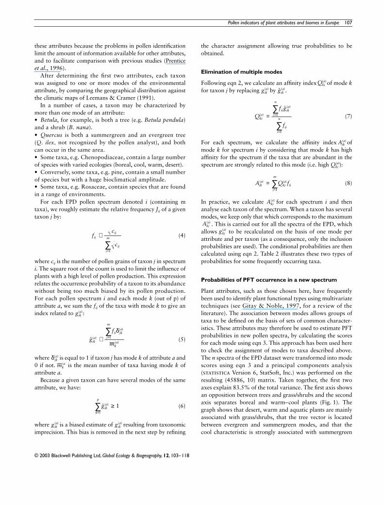
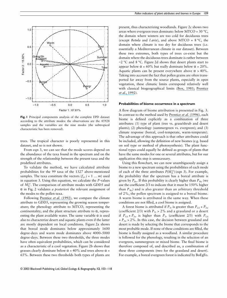
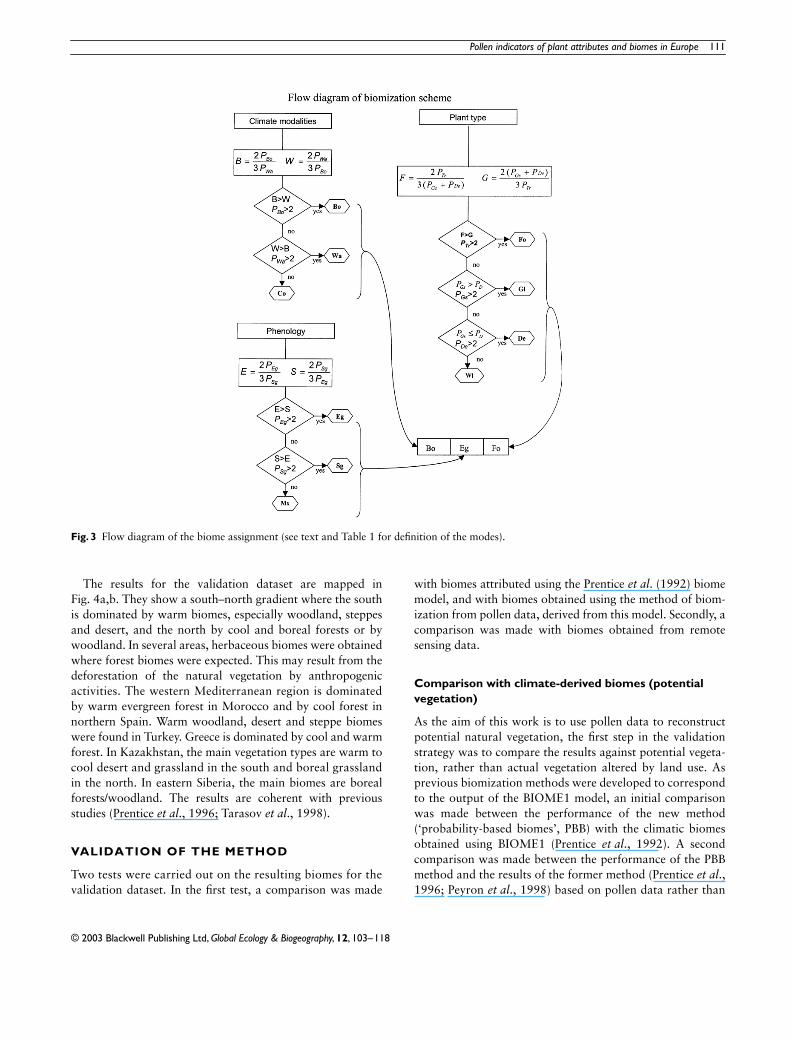
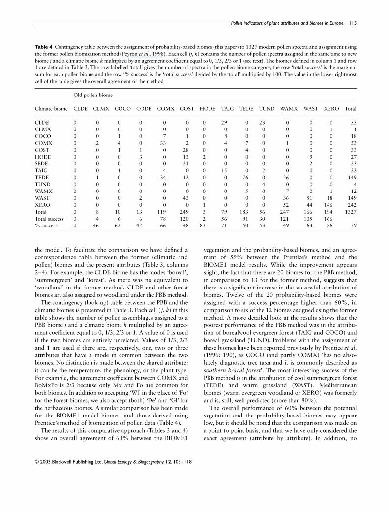
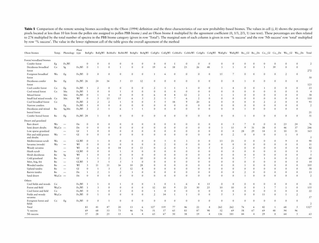
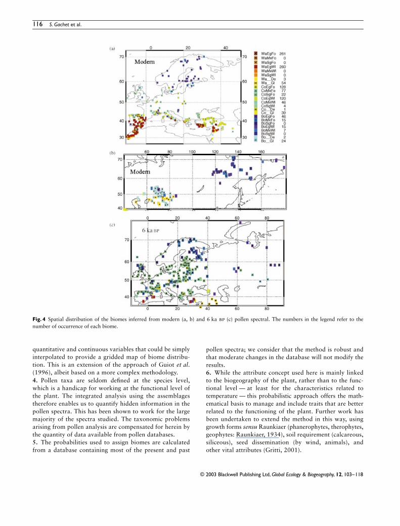