Federal Reserve Bank of Minneapolis

Spring 1994

v A Primer on Static Applied General Equilibrium Models (p. 2) Patrick J. Kehoe Timothy J. Kehoe

i v.

- J 4r o ^ O y j Sir: . UJ ^ gD ui I, i

C " J

L

r -CJ

L i t >

Capturing NAFTA's Impact With Applied General Equilibrium Models (p.17)

Patrick J. Kehoe Timothy J. Kehoe

«T)

Federal Reserve Bank of Minneapolis

Quarterly Review vol 18.no. 2

ISSN 0271-5287

This publication primarily presents economic research aimed at improving policymaking by the Federal Reserve System and other governmental authorities.

Any views expressed herein are those of the authors and not necessarily those of the Federal Reserve Bank of Minneapolis or the Federal Reserve System.

Editor: Arthur J. Rolnick Associate Editors: S. Rao Aiyagari, John H. Boyd, Preston J. Miller,

Warren E. Weber Economic Advisory Board: Richard Rogerson, James A. Schmitz, Jr.

Managing Editor: Kathleen S. Rolfe Article Editors: Kathleen A. Mack, Kathleen S. Rolfe, Martha L. Starr

Designer: Phil Swenson Associate Designer: Beth Leigh Grorud

Typesetter: Jody Fahland Circulation Assistant: Cheryl Vukelich

The Quarterly Review is published by the Research Department of the Federal Reserve Bank of Minneapolis. Subscriptions are available free of charge.

Quarterly Review articles that are reprints or revisions of papers published elsewhere may not be reprinted without the written permission of the original publisher. All other Quarterly Review articles may be reprinted without charge. If you reprint an article, please fully credit the source—the Minneapolis Federal Reserve Bank as well as the Quarterly Review—and include with the reprint a version of the standard Federal Reserve disclaimer (italicized above). Also, please send one copy of any publication that includes a reprint to the Minneapolis Fed Research Department.

Direct all comments and, questions to

Quarterly Review Research Department Federal Reserve Bank of Minneapolis P.O. Box 291 Minneapolis, Minnesota 55480-0291 (612-340-2341 / FAX 612-340-2366).

Federal Reserve Bank of Minneapolis Quarterly Review Spring 1994

A Primer on Static Applied General Equilibrium Models

Patrick J. Kehoe Adviser Research Department Federal Reserve Bank of Minneapolis and Associate Professor of Economics University of Minnesota

Timothy J. Kehoe Adviser Research Department Federal Reserve Bank of Minneapolis and Professor of Economics University of Minnesota

Static applied general equilibrium (AGE) models have been used extensively over the past 20 years to analyze government policies in both developed and less developed countries. (See, for example, Shoven and Whalley 1984, 1992.) Not surprisingly, static AGE models were also the tools of choice when researchers began studying the po-tential impact of the North American Free Trade Agree-ment (NAFTA) on the Canadian, Mexican, and U.S. econ-omies (Francois and Shiells 1994). In another article in this issue, we examine some specific applications of static AGE models to NAFTA. Here, though, we try to describe the basic structure of AGE models and give some sense of their reliability.

In this article, we construct a simple model and use it in a series of examples to explain the structure of static AGE models. We then extend our model to include in-creasing returns to scale, imperfect competition, and dif-ferentiated products, following the trend of AGE modeling over the last 10 years. We also present an example that provides some clues about the reliability of these models. Our example compares a static AGE model's predictions with the actual data on how Spain was affected by enter-ing the European Community (EC) between 1985 and 1986. We find that, at least when exogenous effects are included, a static AGE model's predictions are fairly reli-able.

But these models are not perfect. One reason static AGE models have been so popular is that they stress the

interaction among different industries, or sectors. Because they emphasize the impact of reallocating resources across sectors of an economy, these models are good tools for identifying winners and losers under a policy change. They fail to capture the effect of a policy change on the dynam-ic aspects of an economy, however. A policy change such as NAFTA is likely to directly affect dynamic phenomena such as capital flows, demographics, and growth rates. Here, we merely indicate that, good as they are, static AGE models have their limitations. In our other article in this issue, however, we present some preliminary results which demonstrate that dynamic modeling of the effects of a policy change like NAFTA is an area of research that de-serves more attention.

Basics Like any economic model, an AGE model is an abstrac-tion that is complex enough to capture the essential fea-tures of an economic situation, yet simple enough to be tractable. Our model is a computer representation of a na-tional economy or a group of national economies, each of which consists of consumers, producers, and possibly a government. The consumers in the computer model do many of the same things their counterparts in the world do: They purchase goods from producers, and in return, they supply factors of production. They may also pay tax-es to the government and save part of their income.

To analyze the impact of a change in government poli-

2

Patrick J. Kehoe, Timothy J. Kehoe A Primer on Static AGE Models

cy with a static AGE model, we use the comparative stat-ics methodology: We construct the model so that its equi-librium replicates observed data. We then simulate the pol-icy change by altering the relevant policy parameters and calculating the new equilibrium. Performing policy experi-ments is obviously less costly in a computer economy than in the world economy. But the ultimate value of the pro-cedure depends on how well the model with the simulated policy change predicts what would have happened if the policy change had actually been made.

A Simple Model As the basis for our discussion of alternative modeling strategies and possible uses of AGE models, we begin by sketching out the structure of a highly simplified static model. The model is of the type originally developed by Shoven and Whalley (1972). Consider a model of a single country. Imagine that we have data for all the interindus-try transactions that take place in its economy for one year as well as all payments to factors of production and final demands for goods. Assembled in a matrix, such a data set is an input-output matrix of the sort originally developed by Leontief (1941).

Table 1 contains a simple input-output matrix for the Mexican economy in 1989. All transactions have been ag-gregated under the categories of three industrial sectors: primaries, manufactures, and services. These sectors are highly aggregated. The manufacturing sector, for example, lumps together such diverse goods as processed foods, textiles, and transportation equipment. A model designed to measure the potential impact on different industrial sec-tors of a policy change like NAFTA would have a much finer disaggregation.

All quantities in Table 1 are expressed in tens of tril-lions of 1989 Mexican pesos. In 1989, the exchange rate between pesos and U.S. dollars averaged about 2,400 pe-sos per dollar; for example, 350 trillion pesos in total pri-vate consumption corresponded to about 146 billion dol-lars.

In an input-output matrix, the label on a column indi-cates who made an expenditure, and the label on a row in-dicates who received it. Reading down the second column of Table 1, for example, we see that in 1989, producers of manufacturing goods in Mexico purchased 40 trillion pe-sos of intermediate inputs from producers of primaries and 30 trillion pesos of imports. Reading across the second row, we see that private consumers purchased 110 trillion pesos of manufactures and that 40 trillion pesos of man-

ufactures were exported. The rows and columns of the ma-trix in Table 1 are ordered so that the transactions break down into blocks: intermediate inputs, final demands, and components of the value added. The transactions reported in this input-output matrix are consistent with the figures in the national income account presented in Table 2, which records the Mexican gross domestic product (GDP) in 1989 as being 510 trillion pesos, or about 213 billion dollars.

We construct a static AGE model by inventing artifi-cial consumers, producers, a government, and foreigners who make the same transactions in the base case equilibri-um of the computer economy as do their counterparts in the world. With a large amount of data (for example, a time series of input-output matrices), we could use statisti-cal estimation techniques to find the parameters that char-acterize the people in the artificial economy (Jorgenson 1984).

A more common method for constructing an AGE model is to calibrate its parameters (Mansur and Whalley 1984). Using simple functional forms, we work backward from the data in Table 1 to construct economic agents whose transactions duplicate those observed.

To understand the uses of this sort of model and the procedure used to calibrate it, consider a highly simplified model in which all consumers are identical. To further sim-plify the model, let us aggregate the spending and income of die government with those of the consumers and con-sider a single representative consumer. At this stage, we model the foreign sector not as a separate economic agent but as a production activity with exports as inputs and im-ports as outputs. We later discuss how to model foreign trade in a more sophisticated way. In this economy, six goods are produced: primaries, manufactures, services, an investment good, a government consumption good, and an import good. Each of these goods is produced using inter-mediate inputs of the other goods and two factors of pro-duction: labor and capital.

We assume that the consumer solves a utility-maximi-zation problem of the form

(1) max u(cl9c2,c3,c4,c5,c6)

subject to

(2) pici < (l-x)(wl+rk) + T.

In the utility function, cl9 c2, and c3 are the quantities of primaries, manufactures, and services purchased; c4 is the

3

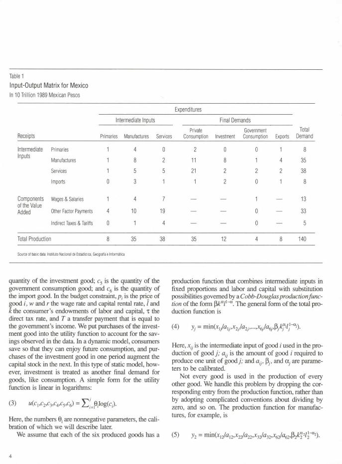
Table 1

Input-Output Matrix for Mexico In 10 Trillion 1989 Mexican Pesos

Expenditures

Intermediate Inputs Final Demands

Receipts Primaries Manufactures Services Private

Consumption Investment Government Consumption Exports

Total Demand

Intermediate Primaries 1 4 0 2 0 0 1 8 Inputs

Manufactures 1 8 2 11 8 1 4 35

Services 1 5 5 21 2 2 2 38

Imports 0 3 1 1 2 0 1 8

Components Wages & Salaries 1 4 7 1 13 of the Value Added Other Factor Payments 4 10 19 — — 0 — 33

Indirect Taxes & Tariffs 0 1 4 — — 0 — 5

Total Production 8 35 38 35 12 4 8 140

Source of basic data: Instituto National de Estadlstica, Geografia e Informatica

quantity of the investment good; c5 is the quantity of the government consumption good; and c6 is the quantity of the import good. In the budget constraint, pl is the price of good i, w and r the wage rate and capital rental rate, / and k the consumer's endowments of labor and capital, x the direct tax rate, and T a transfer payment that is equal to the government's income. We put purchases of the invest-ment good into the utility function to account for the sav-ings observed in the data. In a dynamic model, consumers save so that they can enjoy future consumption, and pur-chases of the investment good in one period augment the capital stock in the next. In this type of static model, how-ever, investment is treated as another final demand for goods, like consumption. A simple form for the utility function is linear in logarithms:

(3) M(c1,C2,C3,C4,C5,C6) = YHjMvtc) .

Here, the numbers 0, are nonnegative parameters, the cali-bration of which we will describe later.

We assume that each of the six produced goods has a

production function that combines intermediate inputs in fixed proportions and labor and capital with substitution possibilities governed by a Cobb-Douglas productionfunc-tion of the form (5kalx~°". The general form of the total pro-duction function is

( 4 ) y j = m m ( x l j / a y , x 2 j / a 2 j , . . . , x 6 j / a 6 j $ j k p l j ~ a j ) .

Here, xtJ is the intermediate input of good i used in the pro-duction of good j; atj is the amount of good / required to produce one unit of good j; and aijf p., and a ; are parame-ters to be calibrated.

Not every good is used in the production of every other good. We handle this problem by dropping the cor-responding entry from the production function, rather than by adopting complicated conventions about dividing by zero, and so on. The production function for manufac-tures, for example, is

(5) y2 = min(x12/a12,x22/a22^32/a32,x62/a62,p2/:22/2~a2)-

4

Patrick J. Kehoe, Timothy J. Kehoe A Primer on Static AGE Models

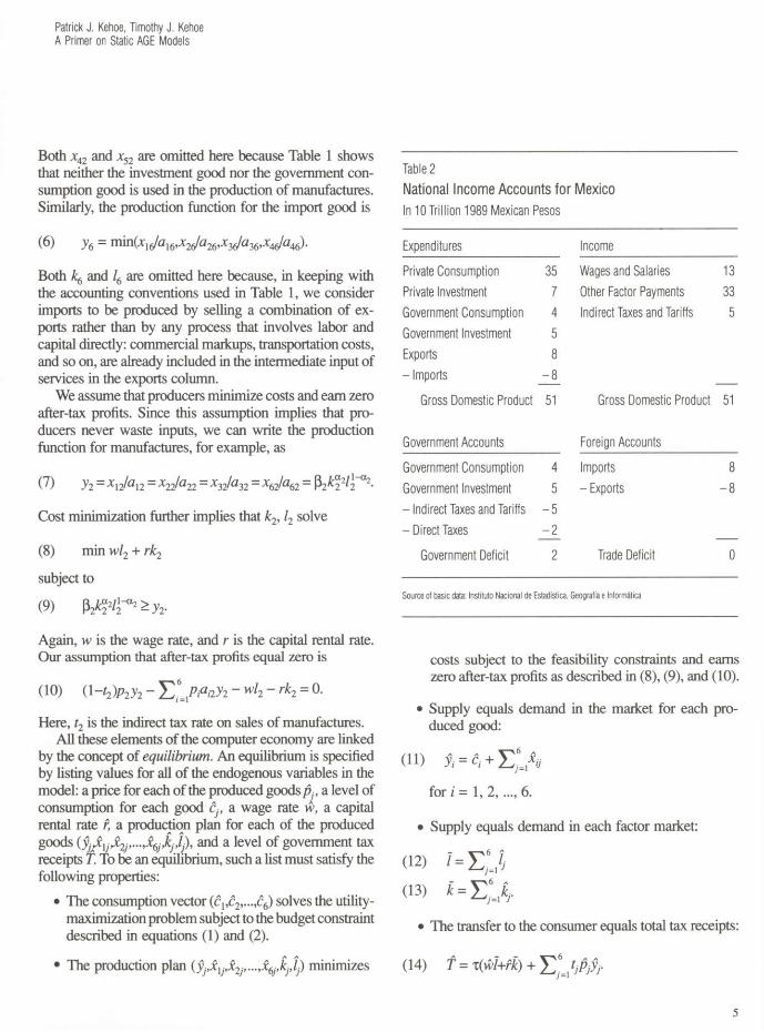
Both x42 and x52 are omitted here because Table 1 shows that neither the investment good nor the government con-sumption good is used in the production of manufactures. Similarly, the production function for the import good is

(6) = rmn(xl6/al6,x26/a26,x36/a36,x46/a46).

Both k6 and /6 are omitted here because, in keeping with the accounting conventions used in Table 1, we consider imports to be produced by selling a combination of ex-ports rather than by any process that involves labor and capital directly: commercial markups, transportation costs, and so on, are already included in the intermediate input of services in the exports column.

We assume that producers minimize costs and earn zero after-tax profits. Since this assumption implies that pro-ducers never waste inputs, we can write die production function for manufactures, for example, as

(7) y2 — X\2I@\2 ~ -̂ 22̂ 22 = ^32^32 = -̂ 62/̂ 62 = P2̂ 22 2̂~<X2'

Cost minimization further implies that k2, l2 solve

(8) min wl2 + rk2

subject to

(9) p r 2 n \ ^ > y 2 .

Again, w is the wage rate, and r is the capital rental rate. Our assumption that after-tax profits equal zero is

(10) (1 -t2)p2y2 - E ^ m - 2 ^ 2 " " = 0.

Here, t2 is the indirect tax rate on sales of manufactures. All these elements of the computer economy are linked

by the concept of equilibrium. An equilibrium is specified by listing values for all of the endogenous variables in the model: a price for each of the produced goods pjf a level of consumption for each good cjf a wage rate w, a capital rental rate r, a production plan for each of the produced goods (SiJcy Jc2j,...,x6j,kj,/y), and a level of government tax receipts f . To be an equilibrium, such a list must satisfy the following properties:

• The consumption vector (cvc2,...,c6) solves the utility-maximization problem subject to the budget constraint described in equations (1) and (2).

• The production plan {yjfxXjyx2j,...,x6j,kjyty minimizes

Table 2

National Income Accounts for Mexico In 10 Trillion 1989 Mexican Pesos

Expenditures Income

Private Consumption 35 Wages and Salaries 13

Private Investment 7 Other Factor Payments 33

Government Consumption 4 Indirect Taxes and Tariffs 5

Government Investment 5

Exports 8

- Imports - 8

Gross Domestic Product 51 Gross Domestic Product 51

Government Accounts Foreign Accounts

Government Consumption 4 Imports 8

Government Investment 5 - Exports - 8

- Ind i rec t Taxes and Tariffs - 5

- Direct Taxes - 2

Government Deficit 2 Trade Deficit 0

Source of basic data: Instituto Nacional de Estadfstica, Geografia e Informatica

costs subject to the feasibility constraints and earns zero after-tax profits as described in (8), (9), and (10).

• Supply equals demand in the market for each pro-duced good:

(11) yi = q + Y , j J i j

for i = 1 , 2 , 6 .

• Supply equals demand in each factor market:

( 1 2 ) I = R J

(B) k = r j r

• The transfer to the consumer equals total tax receipts:

(14) f = x ( w h r k ) ^ Y f l lt M '

5

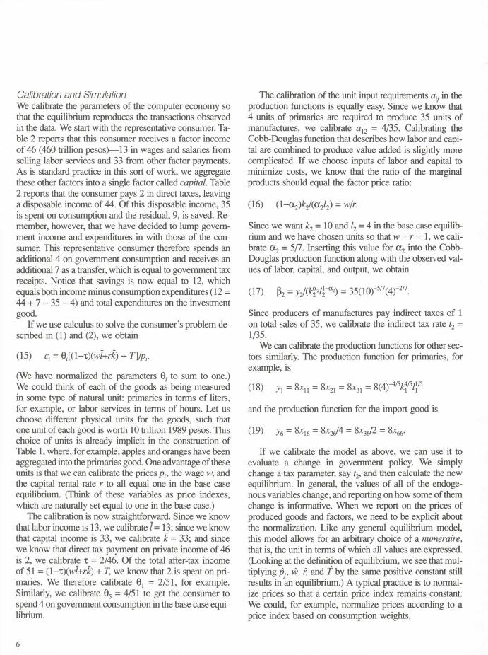
Calibration and Simulation We calibrate the parameters of the computer economy so that the equilibrium reproduces the transactions observed in the data. We start with the representative consumer. Ta-ble 2 reports that this consumer receives a factor income of 46 (460 trillion pesos)—13 in wages and salaries from selling labor services and 33 from other factor payments. As is standard practice in this sort of work, we aggregate these other factors into a single factor called capital. Table 2 reports that the consumer pays 2 in direct taxes, leaving a disposable income of 44. Of this disposable income, 35 is spent on consumption and the residual, 9, is saved. Re-member, however, that we have decided to lump govern-ment income and expenditures in with those of the con-sumer. This representative consumer therefore spends an additional 4 on government consumption and receives an additional 7 as a transfer, which is equal to government tax receipts. Notice that savings is now equal to 12, which equals both income minus consumption expenditures (12 = 44 + 7 - 3 5 - 4 ) and total expenditures on the investment good.

If we use calculus to solve the consumer's problem de-scribed in (1) and (2), we obtain

(15) c -e^ l -T ) (w l+rk) + T]/p,

(We have normalized the parameters 9, to sum to one.) We could think of each of the goods as being measured in some type of natural unit: primaries in terms of liters, for example, or labor services in terms of hours. Let us choose different physical units for the goods, such that one unit of each good is worth 10 trillion 1989 pesos. This choice of units is already implicit in the construction of Table 1, where, for example, apples and oranges have been aggregated into the primaries good. One advantage of these units is that we can calibrate the prices pit the wage w, and the capital rental rate r to all equal one in the base case equilibrium. (Think of these variables as price indexes, which are naturally set equal to one in the base case.)

The calibration is now straightforward. Since we know that labor income is 13, we calibrate I = 13; since we know that capital income is 33, we calibrate k = 33; and since we know that direct tax payment on private income of 46 is 2, we calibrate T = 2/46. Of the total after-tax income of 51 = (1-t)(wl+ric) + Ty we know that 2 is spent on pri-maries. We therefore calibrate = 2/51, for example. Similarly, we calibrate 95 = 4/51 to get the consumer to spend 4 on government consumption in the base case equi-librium.

The calibration of the unit input requirements atJ in the production functions is equally easy. Since we know that 4 units of primaries are required to produce 35 units of manufactures, we calibrate an - 4/35. Calibrating the Cobb-Douglas function that describes how labor and capi-tal are combined to produce value added is slightly more complicated. If we choose inputs of labor and capital to minimize costs, we know that the ratio of the marginal products should equal the factor price ratio:

(16) (l-og/:2/(a2/2) = w/r.

Since we want k2 = 10 and /2 = 4 in the base case equilib-rium and we have chosen units so that w = r - 1, we cali-brate = 5/7. Inserting this value for c^ into the Cobb-Douglas production function along with the observed val-ues of labor, capital, and output, we obtain

(17) fc = y 2 / ( k ^ ) = 35(10)"5/7(4)-2/7.

Since producers of manufactures pay indirect taxes of 1 on total sales of 35, we calibrate the indirect tax rate t2 = 1/35.

We can calibrate the production functions for other sec-tors similarly. The production function for primaries, for example, is

(18) yx = 8jcu = 8jc21 = 8jc31 = 8(4)"4/5^/5/}/5

and the production function for the import good is

(19) j6 = Sxl6 = 8 X2(JA = 8x36/2 = 8 ^ .

If we calibrate the model as above, we can use it to evaluate a change in government policy. We simply change a tax parameter, say t2, and then calculate the new equilibrium. In general, the values of all of the endoge-nous variables change, and reporting on how some of them change is informative. When we report on the prices of produced goods and factors, we need to be explicit about the normalization. Like any general equilibrium model, this model allows for an arbitrary choice of a numeraire, that is, the unit in terms of which all values are expressed. (Looking at the definition of equilibrium, we see that mul-tiplying pj, w, ry and T by the same positive constant still results in an equilibrium.) A typical practice is to normal-ize prices so that a certain price index remains constant. We could, for example, normalize prices according to a price index based on consumption weights,

6

Patrick J. Kehoe, Timothy J. Kehoe A Primer on Static AGE Models

(20) E6e,P, = i. * — = 1

Changes in the wage rate would then be termed changes in the real wage rate.

One of the most interesting results to report is how con-sumer welfare changes. Since utility is expressed in no natural units, economists often choose to measure welfare using an index based on income. A common measure of welfare is how much income the consumer would need, when faced with the base case prices, to achieve the same level of utility as in the simulation. Changes in this mea-sure of welfare are called the equivalent variation.

Additions to the Simple Model In calibrating both the consumer and the producers in our simple model, we have used either Cobb-Douglas or fixed-proportions functions, and therefore all elasticities of sub-stitution are equal to one or infinity. (The utility function is the logarithm of a Cobb-Douglas function.) If informa-tion is available on elasticities of substitution in consump-tion or production, however, it can easily be incorporated into the calibration procedure. Suppose, for example, that we have information from econometric estimates that the elasticity of substitution in consumption is 1/2. Then we need to calibrate the constant elasticity of substitution util-ity function

(21) W(C1,C2,C3,C4,C5,C6) = cj"1/a)°/(a 1}

where a = 1/2 is the elasticity of substitution. Again, we calibrate by working backward from the solution to the utility-maximization problem,

(22) c,- = Q°[(\-T)(wl+ric) + T ] / ( j ^ J P ^ f y

We obtain, for example, the parameter for primaries 0, = 4/727 and the parameter for government consumption 05 = 16/727.

Even if we allow for more flexible functional forms, the model that we have described is highly simplified. In practice, static AGE models allow more disaggregation, more institutional details, and some market imperfections. Models used in policy analysis typically include many more production sectors. They may also include different types of consumer groups, and factors of production may be disaggregated. For example, labor might be broken down by skill level. Unfortunately, data restrictions usual-ly prevent any simple breakdown of the aggregate capital input.

In models that focus on public finance issues, more de-tail usually goes into specifying government tax, transfer, and subsidy systems. Such models also separate govern-ment and private spending decisions, treating the govern-ment as a separate consumer. Government deficits can then be modeled as sales of goods called bonds by the govern-ment to the other consumers. These bonds are regarded by consumers as perfect substitutes for the investment good in their savings decisions. Models that focus on trade is-sues, such as those used to analyze the impact of NAFTA and discussed elsewhere in this issue, include more details on tariffs and quotas. These models may also allow for trade surpluses or deficits by introducing sales or purchas-es of the investment good by the foreign sector. (For ex-planations of the various ways to model government and trade deficits, see Kehoe and Serra-Puche 1983 and Kehoe et al. 1988.) Other models permit the government to set some prices and quantities.

A market imperfection often built into a static AGE model is in the labor market. The real wage, specified in terms of an index of other prices, is typically modeled as being downwardly rigid. Changes in the demand for labor result in varying rates of unemployment. If demand for la-bor rises so much that full employment occurs, the real wage then rises so that supply is equal to demand. (See Kehoe and Serra-Puche 1983.) Another possibility is to fix the return to capital. Then the interpretation involves not unemployment of capital but rather international capital flows. If demand for capital rises, an inflow from the rest of the world occurs. If demand for capital falls, an outflow occurs.

Foreign Trade and the Armington Specification One of the most significant departures from our simple model structure that was taken by models used to analyze NAFTA involves the treatment of foreign trade. An obvi-ous way to model foreign trade is to put a number of sin-gle-country models together and let them interact. Another way, which is frequently found in both theoretical and ap-plied work, simplifies matters by assuming that the coun-try under consideration is so small that it cannot affect the determination of equilibrium in the rest of the world. Em-ploying this small-country assumption, we can treat for-eign prices as exogenous and deal with what is, in effect, a single-country model.

Whether we use a multicountry or a single-country model, we must decide whether goods in the same indus-trial category in different countries are regarded by con-sumers and producers as identical. A specification typical

7

of many AGE trade models is to distinguish goods by in-dustry and by country of origin. Thus, for example, an American-produced automobile is a different good from a Japanese-produced automobile—a close but imperfect substitute.

This specification, named the Armington (1969) speci-fication after the economist who invented it, has three ad-vantages over obvious alternatives for matching the model to data on trade flows. One is that it accounts for the large amount of cross-hauling present in the data, where a coun-try both imports and exports goods of the same product category. In a model where goods are homogeneous, cross-hauling does not exist. Another advantage of this specifi-cation is that it explains the empirical observation that even at a very disaggregated level, most countries produce goods in all product categories. In models where goods are not distinguished by country of origin and produced goods exceed factors of production, countries typically specialize in the production of a limited number of goods. Still another advantage of the Armington specification is that it allows for differing degrees of substitution among domestic and imported goods across different products and allows for changes in the relative prices of different imported goods. Empirical studies indicate that both of these phenomena are found in time series data. (See, for example, Shiells, Stern, and Deardorff 1986.) Neither is possible in a model that aggregates all imports together or in a model that treats domestic and imported goods as per-fect substitutes.

Another approach, based on theoretical work by Dixit and Stiglitz (1977) and Ethier (1982), goes one step fur-ther than the Armington specification and distinguishes a good not by its country of origin but by the firm that pro-duces it. Thus, as a good, a Ford automobile differs from both a Chrysler and a Toyota. As we explain next, differ-entiating goods by firm necessarily requires modeling firms as imperfect competitors. In contrast, differentiating goods by country is not inherently linked to imperfect competition, although imperfect competition is often found in models that employ the Armington specification.

To calibrate a model that employs the Armington spec-ification, we need to arrange the data slightly differently than they are arranged in Table 1. The imports there are classified by the sector that purchases them, the sector of destination, and not by the sector that produces them, the sector of origin. In the manufactures column, for example, the entry of 3 in the imports row indicates total purchases of 30 trillion pesos worth of imports of all types by the

manufactures sector, not total imports of 30 trillion pesos of manufactures. Suppose that we use a different input-output matrix in which imports are classified by sector of origin and find that the value of imports of manufactures in 1989 was 5. Suppose, too, that we have econometric evidence that the elasticity of substitution between domes-tic manufactures and imported manufactures was 3/2. We can then use this information to calibrate an Armington aggregator that combines domestic and imported manu-factures to produce an aggregate manufactured good that is then used as an intermediate input by the production sec-tors, consumed by private consumers or the government, invested, or exported:

(23) >>2 = y2[ + ( l - 6 2 ) ^ r ^ - i > .

Here, y2 is the aggregate of manufactures, y2d is domestic production of manufactures, and y2fis imports. Solving the problem of minimizing the cost of the aggregate good and inserting a2 = 3/2, = 40, y2d = 35, and we can cal-ibrate 82 = 72/3/(l+7/3) and y2 = (l+72/3)3/64. We can simi-larly construct Armington aggregators for primaries and services.

Many models employ the Armington specification in single-country models. A common way to use this specifi-cation is to model the domestic economy as a small coun-try (one that takes prices and incomes in the rest of the world as exogenous). This assumption is not, however, the simple small-country assumption of the traditional trade theory that assumes no product differentiation. According to the Armington specification, domestic goods are differ-ent goods from foreign goods, which allows the prices of domestic goods to vary and gives even the smallest coun-try some market power. (Of course, the higher the substi-tutability between domestic and foreign goods, the lower the flexibility for such fluctuations.) Cox and Harris (1985) refer to this combination of modeling the determination of foreign prices and incomes as exogenous and modeling do-mestic and foreign goods as imperfect substitutes as the al-most small-country assumption. This assumption allows us to analyze trade issues in what is essentially a single-coun-try model but makes the model something less than a full general equilibrium model in which all relevant variables are determined endogenously.

In our simple model, the easiest way to introduce the almost small-country assumption is to specify a foreign consumer who solves the utility-maximization problem

8

Patrick J. Kehoe, Timothy J. Kehoe A Primer on Static AGE Models

(24) max £ ' U o g f e o c ^ + ( l - p ^ ] 0 ^ x—'/ =1 J

subject to

(25) Y,3,JPidxid+ePifxif) = e If

Here, xid is the foreign consumer's consumption of the do-mestic good /, or domestic exports of that good; xifis con-sumption of the foreign good; ptj is the price of the for-eign good; e is a real exchange rate that corresponds to the price of the import good in the simple model; and If is foreign income. The reciprocal of e is often referred to as the domestic country's terms of trade.

A typical specification is to assume that foreign income Ifmd prices of foreign goods pif are exogenous. The mod-el is then closed by letting the real exchange rate e adjust so as to keep trade balanced—the total value of exports equals the total value of imports.

The general equilibrium interpretation of this specifica-tion is that the foreign consumer is endowed with a fixed amount of one of the foreign goods and has access to a production technology that can transform this good into any of the other foreign goods in fixed proportions. The fixed proportions and profit maximization guarantee that the relative prices of the foreign goods are fixed in equilib-rium. The real exchange rate e is now the price of the for-eign good with which the foreign consumer is endowed.

Modifications The simple model in the previous section has constant re-turns in production and perfect competition among produc-ers. This was the dominant model in early AGE analyses of trade policy. (See, for example, Srinivasan and Whalley 1986.) Over the past decade, however, the trend in both theoretical and applied work on trade has been to incor-porate such phenomena as increasing returns to scale as well as imperfect competition and product differentiation. We will now explore the various ways that these phenom-ena can be included in our simple model.

Increasing Returns The first AGE model to include increasing returns along with imperfect competition was developed by Harris (1984) to analyze the impact on Canada of the then-pro-posed U.S.-Canada Free Trade Agreement (FTA). Harris was motivated by empirical work on Canadian manufac-turing, in particular, that of Eastman and Stykolt (1966). They argue that protection in a small economy like Cana-da restricts market size and limits foreign competition in

certain industries, promoting many firms which operate at scales that are too small in terms of economic efficiency. Harris (1984) and Cox and Harris (1985) show that by in-corporating increasing returns and imperfect competition into some industrial sectors of an AGE model, they can capture these effects and thereby identify a much larger impact on Canada of an FTA with the United States. This research played an important role in the political debate in Canada leading up to approval of the agreement.

To show how Harris' model incorporates increasing re-turns and imperfect competition, we will explain how to build these features into the manufactures sector of our simple model while keeping the primaries and services sectors competitive. We begin by considering the produc-tion function for an individual manufacturing firm. (In the model with constant returns, delineation of individual firms is not important; with increasing returns, it is.) We split the inputs required to produce a certain amount of output into two categories: variable inputs and fixed in-puts. We assume, as do all the modelers whose work is discussed here and in the other article in this issue, that variable inputs are proportional to output. These variable inputs include all of the intermediate inputs and some of the labor and capital inputs. Some of the labor and capital inputs, however, are fixed, and these fixed inputs are re-quired to operate the firm at any level of output except ze-ro, where the firm shuts down.

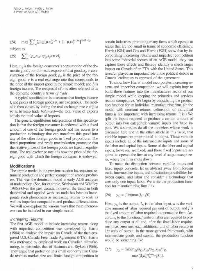
To make the distinction between variable inputs and fixed inputs concrete, let us abstract away from foreign trade, intermediate inputs, and substitution possibilities be-tween capital and labor and consider a technology that uses only one input: labor. We write the production func-tion for manufacturing firm i as

(26) y2i = (l/a)max(/2-/0).

Here, y2i is the output, l2i is the labor input, a is the vari-able amount of labor required per unit of output, and/is the fixed amount of labor required to operate the firm. Ac-cording to this function,/units of labor are required to pro-duce any output at all and, after the fixed-labor require-ment has been met, each additional unit of labor results in 1 /a units of output. In the more general framework, with intermediate goods and capital, the production function would be something like

(27) y2i - mm[xni/al2,x22i/a22,x32i/a32, maxfakf t l^- f ,0)1

9

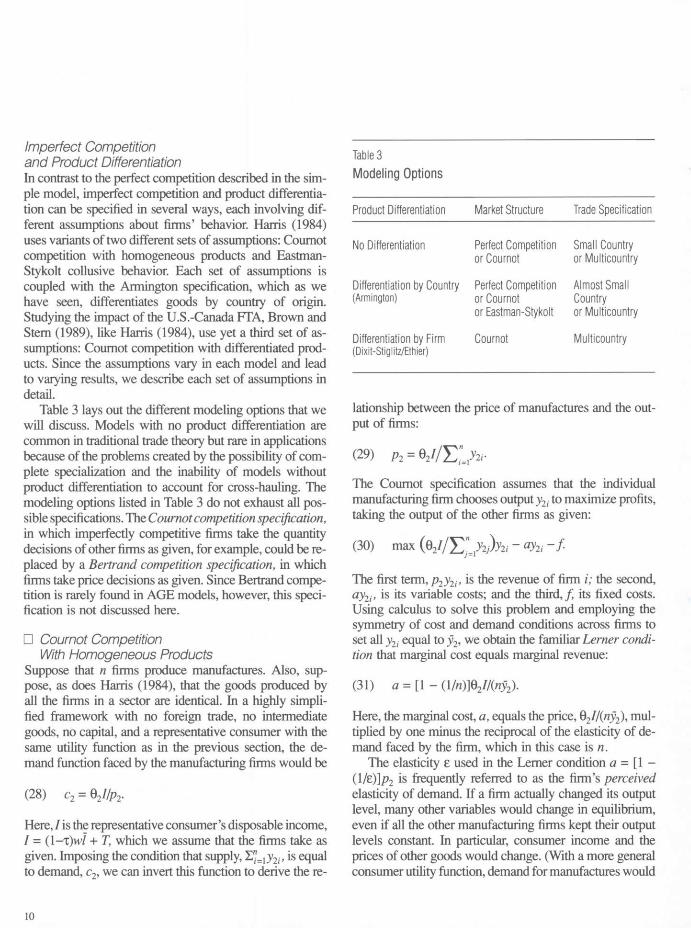
Imperfect Competition and Product Differentiation In contrast to the perfect competition described in the sim-ple model, imperfect competition and product differentia-tion can be specified in several ways, each involving dif-ferent assumptions about firms' behavior. Harris (1984) uses variants of two different sets of assumptions: Cournot competition with homogeneous products and Eastman-Stykolt collusive behavior. Each set of assumptions is coupled with the Armington specification, which as we have seen, differentiates goods by country of origin. Studying the impact of the U.S.-Canada FTA, Brown and Stern (1989), like Harris (1984), use yet a third set of as-sumptions: Cournot competition with differentiated prod-ucts. Since the assumptions vary in each model and lead to varying results, we describe each set of assumptions in detail.

Table 3 lays out the different modeling options that we will discuss. Models with no product differentiation are common in traditional trade theory but rare in applications because of the problems created by the possibility of com-plete specialization and the inability of models without product differentiation to account for cross-hauling. The modeling options listed in Table 3 do not exhaust all pos-sible specifications. The Cournot competition specification, in which imperfectly competitive firms take the quantity decisions of other firms as given, for example, could be re-placed by a Bertrand competition specification, in which firms take price decisions as given. Since Bertrand compe-tition is rarely found in AGE models, however, this speci-fication is not discussed here.

• Cournot Competition With Homogeneous Products

Suppose that n firms produce manufactures. Also, sup-pose, as does Harris (1984), that the goods produced by all the firms in a sector are identical. In a highly simpli-fied framework with no foreign trade, no intermediate goods, no capital, and a representative consumer with the same utility function as in the previous section, the de-mand function faced by the manufacturing firms would be

(28) c2 = 02//p2.

Here, I is the representative consumer's disposable income, I = (1-T)wl + T, which we assume that the firms take as given. Imposing the condition that supply, y2i, is equal to demand, c2, we can invert this function to derive the re-

Table 3 Modeling Options

Product Differentiation Market Structure Trade Specification

No Differentiation Perfect Competition Small Country or Cournot or Multicountry

Differentiation by Country Perfect Competition Almost Small (Armington) or Cournot Country

or Eastman-Stykolt or Multicountry

Differentiation by Firm Cournot Multicountry (Dixit-Stiglitz/Ethier)

lationship between the price of manufactures and the out-put of firms:

(29) p2 = ^ l / Y j i f

The Cournot specification assumes that the individual manufacturing firm chooses output y2i to maximize profits, taking the output of the other firms as given:

(30) max ( e , / / ^ ? ^ / " % "/•

The first term, p2y2i, is the revenue of firm i; the second, ay2i, is its variable costs; and the third,/, its fixed costs. Using calculus to solve this problem and employing the symmetry of cost and demand conditions across firms to set all y2i equal to y2, we obtain the familiar Lerner condi-tion that marginal cost equals marginal revenue:

(31) a = [ 1 - (1 /n)]02//(ny2).

Here, the marginal cost, a, equals the price, 92II(ny2), mul-tiplied by one minus the reciprocal of the elasticity of de-mand faced by the firm, which in this case is n.

The elasticity e used in the Lerner condition a = [1 -(l/e)]p2 is frequently referred to as the firm's perceived elasticity of demand. If a firm actually changed its output level, many other variables would change in equilibrium, even if all the other manufacturing firms kept their output levels constant. In particular, consumer income and the prices of other goods would change. (With a more general consumer utility function, demand for manufactures would

10

Patrick J. Kehoe, Timothy J. Kehoe A Primer on Static AGE Models

depend on these other prices.) Taking these general equi-librium feedbacks of a quantity change into account is a complex technical matter; the feedbacks may even prevent an equilibrium from existing in the model. Since these feedbacks are usually presumed to be small if individual firms are small relative to the economy as a whole, they are generally ignored both in theory and in practice.

To use the Lerner condition to determine the price of manufactures, we must determine the number of firms in the manufactures sector, a?. If we assume free entry and exit of firms in this sector, then the number of firms ad-justs so that profits equal zero. To determine n, we use the profit-maximization condition to solve for _y2 and p2 as functions of n,

(32) j2 = Q2I(n-l)/(an2)

(33) p2 = an/(n-l)

and then insert these formulas into the condition that prof-its equal zero:

(34) Q2I/n - Q2I(n-\)/n2 - / = 0

(35) n = (9 2I/f)m.

In general equilibrium calculations, of course, consumer income varies endogenously, but the above equations com-pletely describe the pricing and output decisions of man-ufacturing firms and the number of such firms. Similar but more complicated expressions describe the corresponding relationships in the more general model.

When calibrating an AGE model with imperfect com-petition to reproduce a base case data set, we can always specify that n is an integer. A potential problem with sim-ulations, however, is that the number emerging from this calculation need not be an integer. Modelers usually deal with this problem by simply ignoring it and reporting whatever number emerges.

• Eastmari-Stykolt Collusive Behavior Harris (1984) considers an alternative to the Cournot spec-ification that he calls the Eastman-Stykolt assumption. Rather than deriving firms' actions as solutions to maxi-mization problems, the Eastman-Stykolt assumption states simply that the domestic price for a good should equal the foreign price multiplied by one plus the domestic tariff. This assumption is based on evidence found by Eastman and Stykolt (1966) that prices in Canadian manufacturing

tended to equal the U.S. prices for similar goods, with ad-justments for tariff protection. Harris thinks that the East-man-Stykolt assumption is fairly appropriate for a small country. He uses the empirical evidence of Eastman and Stykolt to justify the assumption that Canadian firms col-lude in setting prices because they regard the tariff-adjust-ed price of U.S. goods as a sort of focal point, a high price that is easy to monitor and adjust to.

In our simple example, the Eastman-Stykolt assump-tion states that

(36) p2d = (1 +t2)p2f.

Here, p2d is the domestic price of manufactures, t2 is the tariff, and p2f is the foreign price of manufactures, which, as we have mentioned, is exogenous. Unlike with the Cournot specification, we cannot ignore foreign trade in explaining the role of the Eastman-Stykolt assumption. Let us therefore construct Armington aggregators for pri-maries, manufactures, and services. With a utility function that is linear in the logarithms of the three Armington ag-gregates, savings, and government consumption, we can then derive total consumer demand for domestic manufac-tures by solving the utility-maximization problem

(37) max J ^ J M ^ ' + { l ^ ^ Y * ^ + 94log(c4) + 95log(c5)

subject to

(38) Yj]=l[PidCid + + PACA + Psc5 ^ L

Here, cid is consumer demand for the domestic version of good i, and cif is consumer demand for the imported ver-sion.

Using calculus to solve the consumer's utility-maximi-zation problem, imposing the Eastman-Stykolt assumption in the manufactures sector, and adding the demand for do-mestic manufactures by foreigners, we obtain total demand for domestic manufactures y2d. Since we know the price (1 +t2)p2f, we can use the zero-profit condition (which equates price and average costs) to determine average firm output y2:

(39) (1 +t2)p2f = a+f/y2

(40) y2=f/[(l+t2)p2f-a].

This calculation is illustrated in the average cost curve di-

l l

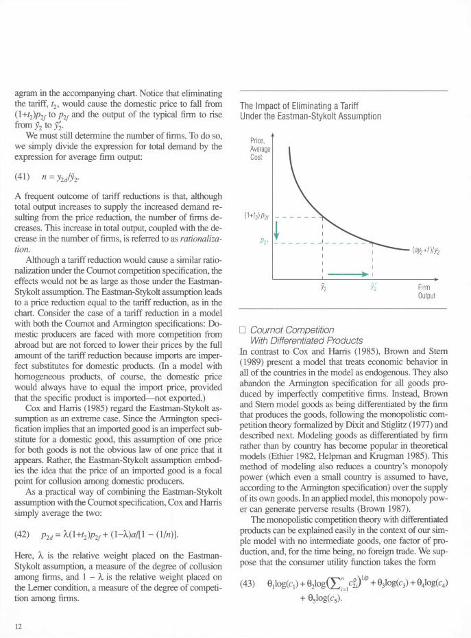
agram in the accompanying chart. Notice that eliminating the tariff, t2, would cause the domestic price to fall from (l+t2)p2f to p2f and the output of the typical firm to rise from y2 to y2.

We must still determine the number of firms. To do so, we simply divide the expression for total demand by the expression for average firm output:

(41) n=y2d/y2.

A frequent outcome of tariff reductions is that, although total output increases to supply the increased demand re-sulting from the price reduction, the number of firms de-creases. This increase in total output, coupled with the de-crease in the number of firms, is referred to as rationaliza-tion.

Although a tariff reduction would cause a similar ratio-nalization under the Cournot competition specification, the effects would not be as large as those under the Eastman-Stykolt assumption. The Eastman-Stykolt assumption leads to a price reduction equal to the tariff reduction, as in the chart. Consider the case of a tariff reduction in a model with both the Cournot and Armington specifications: Do-mestic producers are faced with more competition from abroad but are not forced to lower their prices by the full amount of the tariff reduction because imports are imper-fect substitutes for domestic products. (In a model with homogeneous products, of course, the domestic price would always have to equal the import price, provided that the specific product is imported—not exported.)

Cox and Harris (1985) regard the Eastman-Stykolt as-sumption as an extreme case. Since the Armington speci-fication implies that an imported good is an imperfect sub-stitute for a domestic good, this assumption of one price for both goods is not the obvious law of one price that it appears. Rather, the Eastman-Stykolt assumption embod-ies the idea that the price of an imported good is a focal point for collusion among domestic producers.

As a practical way of combining the Eastman-Stykolt assumption with the Cournot specification, Cox and Harris simply average the two:

(42) Pld=x(\+t2)p2f+(1-ami - m i

Here, X is the relative weight placed on the Eastman-Stykolt assumption, a measure of the degree of collusion among firms, and 1 - X is the relative weight placed on the Lerner condition, a measure of the degree of competi-tion among firms.

The Impact of Eliminating a Tariff Under the Eastman-Stykolt Assumption

Output

• Cournot Competition With Differentiated Products

In contrast to Cox and Harris (1985), Brown and Stem (1989) present a model that treats economic behavior in all of the countries in the model as endogenous. They also abandon the Armington specification for all goods pro-duced by imperfectly competitive firms. Instead, Brown and Stem model goods as being differentiated by the firm that produces the goods, following the monopolistic com-petition theory formalized by Dixit and Stiglitz (1977) and described next. Modeling goods as differentiated by firm rather than by country has become popular in theoretical models (Ethier 1982, Helpman and Krugman 1985). This method of modeling also reduces a country's monopoly power (which even a small country is assumed to have, according to the Armington specification) over the supply of its own goods. In an applied model, this monopoly pow-er can generate perverse results (Brown 1987).

The monopolistic competition theory with differentiated products can be explained easily in the context of our sim-ple model with no intermediate goods, one factor of pro-duction, and, for the time being, no foreign trade. We sup-pose that the consumer utility function takes the form

(43) e^og(Cl)+e2iog(£;=c2p)I/p+03iog(c3)+e4iog(c4) + e5iog(c5).

12

Patrick J. Kehoe, Timothy J. Kehoe A Primer on Static AGE Models

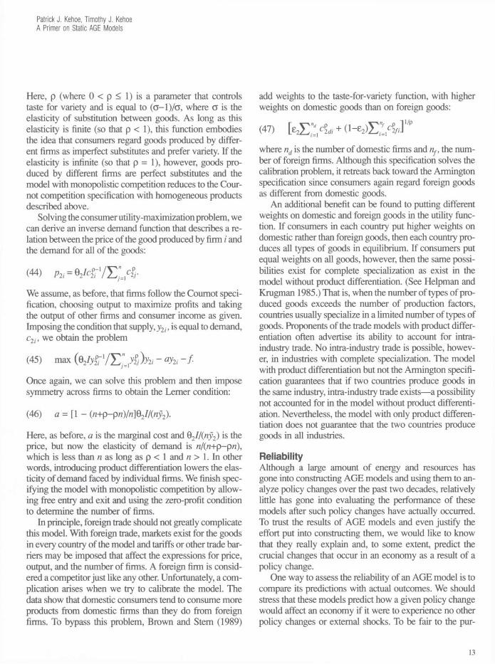
Here, p (where 0 < p < 1) is a parameter that controls taste for variety and is equal to (o-1)/g, where a is the elasticity of substitution between goods. As long as this elasticity is finite (so that p < 1), this function embodies the idea that consumers regard goods produced by differ-ent firms as imperfect substitutes and prefer variety. If the elasticity is infinite (so that p = 1), however, goods pro-duced by different firms are perfect substitutes and the model with monopolistic competition reduces to the Cour-not competition specification with homogeneous products described above.

Solving the consumer utility-maximization problem, we can derive an inverse demand function that describes a re-lation between the price of the good produced by firm i and the demand for all of the goods:

(44) fti = 0 2 / c £ - I / E " . I ^ -

We assume, as before, that firms follow the Cournot speci-fication, choosing output to maximize profits and taking the output of other firms and consumer income as given. Imposing the condition that supply, y2i, is equal to demand, c2i, we obtain the problem

(45) max falyfr1/^J^i " <%, " / •

Once again, we can solve this problem and then impose symmetry across firms to obtain the Lerner condition:

(46) a = [1 - (n+p-pn)/n]Q2I/(ny2).

Here, as before, a is the marginal cost and Q2I/(ny2) is the price, but now the elasticity of demand is n/(n+p-pn\ which is less than n as long as p < 1 and n > 1. In other words, introducing product differentiation lowers the elas-ticity of demand faced by individual firms. We finish spec-ifying the model with monopolistic competition by allow-ing free entry and exit and using the zero-profit condition to determine the number of firms.

In principle, foreign trade should not greatly complicate this model. With foreign trade, markets exist for the goods in every country of the model and tariffs or other trade bar-riers may be imposed that affect the expressions for price, output, and the number of firms. A foreign firm is consid-ered a competitor just like any other. Unfortunately, a com-plication arises when we try to calibrate the model. The data show that domestic consumers tend to consume more products from domestic firms than they do from foreign firms. To bypass this problem, Brown and Stem (1989)

add weights to the taste-for-variety function, with higher weights on domestic goods than on foreign goods:

(47) [ e a E ^ + d - ^ I M *

where nd is the number of domestic firms and nf, the num-ber of foreign firms. Although this specification solves the calibration problem, it retreats back toward the Armington specification since consumers again regard foreign goods as different from domestic goods.

An additional benefit can be found to putting different weights on domestic and foreign goods in the utility func-tion. If consumers in each country put higher weights on domestic rather than foreign goods, then each country pro-duces all types of goods in equilibrium. If consumers put equal weights on all goods, however, then the same possi-bilities exist for complete specialization as exist in the model without product differentiation. (See Helpman and Krugman 1985.) That is, when the number of types of pro-duced goods exceeds the number of production factors, countries usually specialize in a limited number of types of goods. Proponents of the trade models with product differ-entiation often advertise its ability to account for intra-industry trade. No intra-industry trade is possible, howev-er, in industries with complete specialization. The model with product differentiation but not the Armington specifi-cation guarantees that if two countries produce goods in the same industry, intra-industry trade exists—a possibility not accounted for in the model without product differenti-ation. Nevertheless, the model with only product differen-tiation does not guarantee that the two countries produce goods in all industries.

Reliability Although a large amount of energy and resources has gone into constructing AGE models and using them to an-alyze policy changes over the past two decades, relatively little has gone into evaluating the performance of these models after such policy changes have actually occurred. To trust the results of AGE models and even justify the effort put into constructing them, we would like to know that they really explain and, to some extent, predict the crucial changes that occur in an economy as a result of a policy change.

One way to assess the reliability of an AGE model is to compare its predictions with actual outcomes. We should stress that these models predict how a given policy change would affect an economy if it were to experience no other policy changes or external shocks. To be fair to the pur-

13

pose of the models when evaluating their performance af-ter a policy change, we would have to rerun them, includ-ing any other significant policy changes or external shocks that had occurred. The AGE modelers of the U.S.-Canada FTA complain that comparing their predictions with the economic experience of the last several years is difficult because of the recession in both countries. Modelers of the U.S.-Canada FTA, such as Cox and Harris (1985) and Brown and Stern (1989), should rerun their models, how-ever, taking explicit account of how the external shocks affected the United States and Canada in 1989 and after-ward.

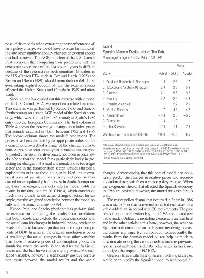
Since no one has carried out this exercise with a model of the U.S.-Canada FTA, we report on a related exercise. This exercise was performed by Kehoe, Polo, and Sancho (forthcoming) on a static AGE model of the Spanish econ-omy, which was built in 1984-85 to analyze Spain's 1986 entry into the European Community. The first column of Table 4 shows the percentage changes in relative prices that actually occurred in Spain between 1985 and 1986. The second column shows the model's predictions. The prices have been deflated by an appropriate index so that a consumption-weighted average of the changes sums to zero. As we have seen, these types of models are designed to predict changes in relative prices, not those in price lev-els. Notice that the model fares particularly badly in pre-dicting the changes in the food and nonalcoholic beverages sector and in the transportation sector. Obvious historical explanations exist for these failings: in 1986, the interna-tional price of petroleum fell sharply and poor weather caused an exceptionally bad harvest in Spain. Incorporat-ing these two exogenous shocks into the model yields the results in the third column of Table 4, which correspond much more closely to the actual changes. Notice, for ex-ample, that the weighted correlation between the model re-sults and the actual changes is 0.94.

Kehoe, Polo, and Sancho (forthcoming) perform simi-lar exercises in comparing the results from simulations that both include and exclude the exogenous shocks with the actual data for changes in industrial prices, production levels, returns to factors of production, and major compo-nents of GDP. In general, the original simulation is better at predicting the actual changes in these other variables than those in relative prices of consumption goods; the simulation where the model is adjusted for the fall in oil prices and the bad harvest does slightly worse. For each set of variables, however, a significantly positive correla-tion exists between the model results and the actual

Table 4

Spanish Model's Predictions vs.The Data Percentage Change in Relative Price, 1985-86*

Model

Sector Actual Original Adjusted

1. Food and Nonalcoholic Beverages 1.8 - 2 . 3 1.7

2. Tobacco and Alcoholic Beverages 3.9 2.5 5.8

3. Clothing 2.1 5.6 6.6

4. Housing - 3 . 2 - 2 . 2 - 4 . 8

5. Household Articles .1 2.2 2.9

6. Medical Services - . 7 - 4 . 8 - 4 . 2

7. Transportation - 4 . 0 2.6 - 6 . 6

8. Recreation - 1 . 4 - 1 . 3 .1

9. Other Services 2.9 1.1 2.8

Weighted Correlation With 1 9 8 5 - 8 6 t 1.000 - .079 .936

*The change in the sectoral price index is deflated by an appropriate aggregate price index. tWeighted correlation coefficients are shown with actual changes in 1985-86. The weights used for each

sector are (1) 0.2540, (2) 0.0242, (3) 0.0800, (4) 0.1636, (5) 0.0772, (6) 0.0376, (7) 0.1342, (8) 0.0675, and (9) 0.1617; these are the consumption shares in the model's benchmark year, which is 1980. Source: Kehoe, Polo, and Sancho, forthcoming

changes, demonstrating that this sort of model can accu-rately predict the changes in relative prices and resource allocation that result from a major policy change. When the exogenous shocks that affected the Spanish economy in 1986 are omitted, however, the model does not fare as well.

The major policy change that occurred in Spain in 1986 was a tax reform that converted most indirect taxes to a value-added tax, in accord with EC requirements. The pro-cess of trade liberalization began in 1986 and is captured in the model. Unlike the modeling exercises presented here and in the other article in this issue, however, the work on Spain did not concentrate on trade issues involving increas-ing returns and imperfect competition. Consequently, the results from the Spanish model do not help us much to discriminate among the various model structures previous-ly discussed and those used in the other article in this issue, to analyze the impact of NAFTA.

One way to evaluate these different modeling strategies would be to modify the Spanish model to incorporate al-

14

Patrick J. Kehoe, Timothy J. Kehoe A Primer on Static AGE Models

ternative assumptions about product differentiation, returns to scale, and market structure. Alternative versions of the model could then be used to "predict" the impact of the trade liberalization that has occurred in Spain in recent years, and the results could be compared with the data. Similarly, the different models used to analyze the impact of NAFTA could be evaluated by using them to "predict" the impact of the policy changes and exogenous shocks that have buffeted the three North American economies over the past decade. In any case, now that NAFTA has been implemented, we will be able to tell, in less than a decade, which models were better at predicting NAFTA's effects.

Although static AGE models like the Spanish model can accurately show how resources are reallocated across sectors as a result of tax or trade policy reform, this em-phasis on sectoral detail has a cost. That cost is the exclu-sion of phenomena that involve time and uncertainty, such as labor market adjustments, capital flows, and growth. For example, for Spain, one of the most significant im-pacts of joining the EC was that foreign investment in-creased. For the six years before Spain joined the EC in 1986, that country averaged $1.5 billion per year in for-eign investment; in the six years after it joined, Spain av-eraged $12.8 billion (International Monetary Fund 1992). Static AGE models can analyze the sectoral impact of such capital flows, but they cannot accurately analyze the deter-minants or predict the size of such flows. For that, a model must incorporate time and uncertainty in investment deci-sions—in short, it must be dynamic.

Concluding Remarks In this article, we have developed a fairly simple applied general equilibrium (AGE) model, extended that model, and then tested to see how well it predicted the economic changes caused by Spain's entry into the European Com-munity. Our results seem to confirm that the strength of static AGE models lies in their ability to predict which in-dustries will benefit and which will falter under such a policy change. Of course, as we noted during our discus-sion of the Spanish example, these models also have some weaknesses; their inability to account for dynamic eco-nomic phenomena is certainly primary among them.

For a look at the application of static AGE models to a specific policy change or reform, turn to our other article in this issue. There, we examine how researchers have used static AGE models to attempt to predict the effects of the North American Free Trade Agreement on the econo-

mies of Canada, Mexico, and the United States. In that article, we also try to provide some insights into the po-tential benefits of dynamically modeling the effects of this policy change.

15

References

Armington, Paul S. 1969. A theory of demand for products distinguished by place of production. International Monetary Fund Staff Papers 16 (March): 159—78.

Brown, Drusilla K. 1987. Tariffs, the terms of trade, and national product differentia-tion. Journal of Policy Modeling 9 (Fall): 503-26.

Brown, Drusilla K., and Stem, Robert M. 1989. U.S.-Canada bilateral tariff elimina-tion: The role of product differentiation and market structure. In Trade policies for international competitiveness, ed. Robert C. Feenstra, pp. 217-45. Chicago: University of Chicago Press.

Cox, David, and Harris, Richard. 1985. Trade liberalization and industrial organization: Some estimates for Canada. Journal of Political Economy 93 (February): 115-45.

Dixit, Avinash K., and Stiglitz, Joseph E. 1977. Monopolistic competition and optimum product diversity. American Economic Review 67 (June): 297-308.

Eastman, Harry C., and Stykolt, Stefan. 1966. The tariff and competition in Canada. Toronto: University of Toronto Press.

Ethier, Wilfred J. 1982. National and international returns to scale in the modem theory of international trade. American Economic Review 72 (June): 389-405.

Francois, Joseph F., and Shiells, Clinton R„ eds. 1994. Modeling trade policy: Applied general equilibrium assessments of NAFTA. Cambridge: Cambridge University Press.

Harris, Richard. 1984. Applied general equilibrium analysis of small open economies with scale economies and imperfect competition. American Economic Review 74 (December): 1016-32.

Helpman, Elhanan, and Krugman, Paul R. 1985. Market structure and foreign trade: Increasing returns, imperfect competition, and the international economy. Cam-bridge, Mass.: MIT Press.

International Monetary Fund. 1992. International financial statistics yearbook. Wash-ington, D.C.: International Monetary Fund.

Jorgenson, Dale W. 1984. Econometric methods for applied general equilibrium analy-sis. In Applied general equilibrium analysis, ed. Herbert E. Scarf and John B. Shoven, pp. 139-203. Cambridge: Cambridge University Press.

Kehoe, Timothy J.; Manresa, Antonio; Noyola, Pedro J.; Polo, Clemente; and Sancho, Ferran. 1988. A general equilibrium analysis of the 1986 tax reform in Spain. European Economic Review 32 (March): 334-42.

Kehoe, Timothy J.; Polo, Clemente; and Sancho, Ferran. Forthcoming. An evaluation of the performance of an applied general equilibrium model of the Spanish economy. Economic Theory. Also 1992. Research Department Working Paper 480. Federal Reserve Bank of Minneapolis.

Kehoe, Timothy J., and Serra-Puche, Jaime. 1983. A computational general equilibrium model with endogenous unemployment: An analysis of the 1980 fiscal reform in Mexico. Journal of Public Economics 22 (October): 1-26.

Leontief, Wassily W. 1941. The structure of American economy, 1919-1929: An em-pirical application of equilibrium analysis. Cambridge, Mass.: Harvard Univer-sity Press.

Mansur, Ahsan Habib, and Whalley, John. 1984. Numerical specification of applied general equilibrium models: Estimation, calibration, and data. In Applied general equilibrium analysis, ed. Herbert E. Scarf and John B. Shoven, pp. 69-127. Cambridge: Cambridge University Press.

Shiells, Clinton R.; Stem, Robert M.; and Deardorff, Alan V. 1986. Estimates of the elasticities of substitution between imports and home goods for the United States. Weltwirtschaftliches-Archiv 122, 497-519.

Shoven, John B., and Whalley John. 1972. A general equilibrium calculation of the ef-fects of differential taxation of income from capital in the U.S. Journal of Public Economics 1 (November): 281-321.

. 1984. Applied general equilibrium models of taxation and international trade: An introduction and survey. Journal of Economic Literature 22 (Septem-ber): 1007-51.

. 1992. Applying general equilibrium. Cambridge: Cambridge University Press.

Srinivasan, T. N., and Whalley, John, eds. 1986. General equilibrium trade policy mod-eling. Cambridge, Mass.: MIT Press.

16