ARTICLE IN PRESS

Reliability Engineering and System Safety 94 (2009) 1618–1628

Contents lists available at ScienceDirect

Reliability Engineering and System Safety

0951-83

doi:10.1

� Corr

E-m

journal homepage: www.elsevier.com/locate/ress

A practical procedure for the selection of time-to-failure models based on theassessment of trends in maintenance data

D.M. Louit a, R. Pascual b,�, A.K.S. Jardine c

a Komatsu Chile, Av. Americo Vespucio 0631, Quilicura, Santiago, Chileb Centro de Minerıa, Pontificia Universidad Catolica de Chile, Av. Vicuna Mackenna 4860, Santiago, Chilec Department of Mechanical and Industrial Engineering, University of Toronto, 5 King’s College Road, Toronto, Ont., Canada M5S 3G8

a r t i c l e i n f o

Article history:

Received 24 April 2008

Received in revised form

6 April 2009

Accepted 10 April 2009Available online 18 April 2009

Keywords:

Trend testing

Time to failure

Model selection

Repairable systems

NHPP

20/$ - see front matter & 2009 Elsevier Ltd. A

016/j.ress.2009.04.001

esponding author.

ail address: rpascual@ing.puc.cl (D.M. Louit).

a b s t r a c t

Many times, reliability studies rely on false premises such as independent and identically distributed

time between failures assumption (renewal process). This can lead to erroneous model selection for the

time to failure of a particular component or system, which can in turn lead to wrong conclusions and

decisions. A strong statistical focus, a lack of a systematic approach and sometimes inadequate

theoretical background seem to have made it difficult for maintenance analysts to adopt the necessary

stage of data testing before the selection of a suitable model. In this paper, a framework for model

selection to represent the failure process for a component or system is presented, based on a review of

available trend tests. The paper focuses only on single-time-variable models and is primarily directed to

analysts responsible for reliability analyses in an industrial maintenance environment. The model

selection framework is directed towards the discrimination between the use of statistical distributions

to represent the time to failure (‘‘renewal approach’’); and the use of stochastic point processes

(‘‘repairable systems approach’’), when there may be the presence of system ageing or reliability

growth. An illustrative example based on failure data from a fleet of backhoes is included.

& 2009 Elsevier Ltd. All rights reserved.

1. Introduction

As described by Dekker and Scarf [1] maintenance optimiza-tion consists of mathematical models aimed at finding balancesbetween costs and benefits of maintenance, or the most appro-priate moment to execute maintenance. Many times, thesemodels are fairly complex and maintenance analysts have beenslow to apply them, since often data are scarce or, due to lack ofstatistical theoretical knowledge, models are very difficult toimplement correctly in an industrial setting. Other, morequalitative techniques such as reliability centered maintenance(RCM) or total productive maintenance (TPM) have then played animportant role in maintenance optimization. Nevertheless, dataanalysis and statistical modeling are definitely very valuable toolsengineers can employ to optimize the maintenance of assetsunder their supervision.

Acknowledging that many reliability studies or maintenanceoptimization programs do not require sophisticated statisticalinputs, Ansell and Phillips [2] reinforce that even at a basic level,we should always be critical of the analysis and ask whether atechnique is appropriate.

ll rights reserved.

The gap between researchers and practitioners of maintenancehas resulted in the fact that although many models rely on veryspecific assumptions for their proper application, these are notnormally discriminated by the practitioner according to the realoperating conditions of their plants or fleets, i.e. real-world data[3,22,43]. O’Connor (cited in [2]) points out that much reliabilityanalysis is done under false premises such as independence ofcomponents, constant failure rates, identically distributed vari-ables, etc. As critical constituents of any reliability analysis, time-to-failure models are not excluded of this situation; thus manytimes the use of conventional time-to-failure analysis techniquesis adopted when they are, in fact, not appropriate.

The aim of this paper is to provide practitioners with a reviewof techniques useful for the selection of a suitable time-to-failuremodel, specifically looking at the case when the standard use ofstatistical distributions is useless, given the presence of long-termtrends in the maintenance failure data. The paper focuses on theselection of single time variable models, since they are the mostcommonly applied in practice, rather than in more complexmultivariate models such as the proportional hazards model,which have also shown great value in their application tomaintenance and reliability [3].

The above does not imply that we propose that time-to-failuremodels should be the center of attention in a reliabilityimprovement study; on the contrary, they should only act as a

ARTICLE IN PRESS

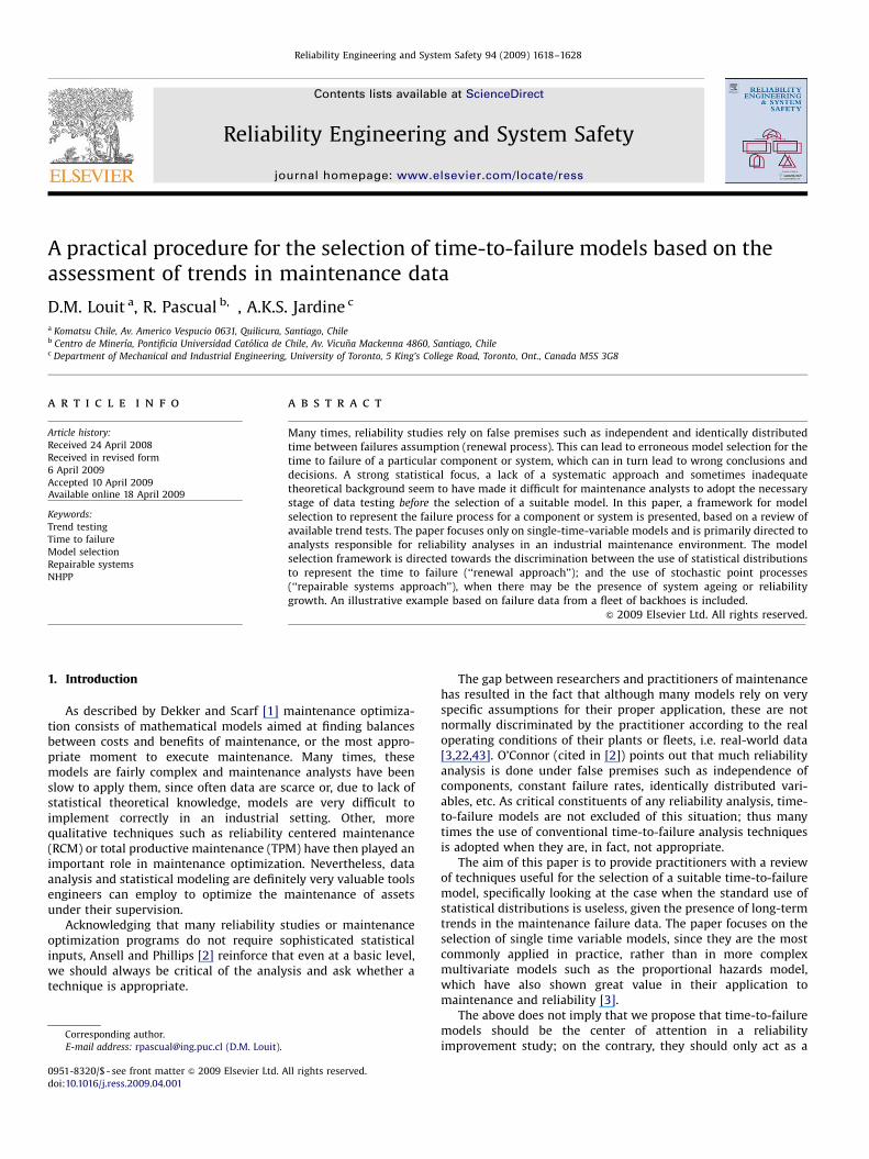
Objectives

Maintenance Data

Model Selection Failure Process

Optimization Model

Solution

Fig. 1. General framework in a reliability improvement study (modified from [2]).

D.M. Louit et al. / Reliability Engineering and System Safety 94 (2009) 1618–1628 1619

tool for the objective the engineers assign to it. Actually, thelogical priority is that of objective, data and, finally, modelselection (as shown in Fig. 1). In other words, as suggested byAnsell and Phillips [4] an analysis should be problem led ratherthan technique or model centered. Nevertheless, correctassessment of the failure process and of time to failure isusually of critical importance to the (posterior) economicanalysis required to find an optimal solution to the problem thatoriginated the analysis. Discussion of approaches to maintenanceand reliability optimization and models mixing reliability andeconomics can be found in several references, for example [5–7].

When dealing with reliability field data, frequently somepractical problems such as the unavailability of large sets of dataoccur. This paper will briefly touch on this and other problems, asthey are relevant to the discussion of model selection techniques.

This document is structured as follows. Section 2 refers tocommon practical problems found in the analysis of reliabilitydata. Section 3 describes the concept of repairable systems andidentifies some of the models available for their representation.Section 4 presents a series of graphical and analytical tests used todetermine the existence of trends in the data. Section 5 proposes aprocedure based on these tests to correctly select a time-to-failuremodel, discriminating between a renewal approach and the use ofan alternative, non-stationary model, such as the non-homo-geneous Poisson process (NHPP). Section 6 presents numericalexamples using data coming from a fleet of backhoes. Finally,Section 7 contains a summary of the paper.

2. Some practical problems in reliability data

2.1. Scarce data

One major problem associated with reliability data is,ironically, the lack of sufficient data to properly run statisticalanalyses, as many authors mentioned repeatedly. In fact, Bendell[8] points out that all statistical methodologies are limited whendone based on small data sets, since the amount of informationcontained by such sets is by nature small. Furthermore, asmentioned in [9], empirical evidences indicate that sets of failuretimes typically contain ten or fewer observations, which empha-size the need to develop methods to deal adequately with smalldata sets (naturally the larger the data set, the more precise thestatistical analysis). Also, many data sets are collected formaintenance management rather than reliability. Hence theinformation content is often very poor and can be misleadingwithout careful scrutiny of the material and cleaning if necessary.

Thomas, a discussant of Ansell and Phillips [10], states that theinsufficient data quantity problem would never disappear, since asthe aim of maintenance is to make failures rare events, one couldexpect that as maintenance improves, fewer failures should occur.Thus the solution, he says, is based on better a priori modeling.Bayesian techniques, directed to incorporate into the models allthe prior information available, are useful in this case. Barlow andProschan [11], Lindley and Singpurwalla [12], Singpurwalla [13],Walls and Quigley [44] and Guikema and Pate-Cornell [45] arerelevant sources for Bayesian methods in reliability.

Although it escapes the reach of this paper, it is valuable tomention Bayesian analysis, because it provides a means to reachoptimal decisions, using standard models as the ones discussedlater on in this paper, when lack of data is a problem. In simplewords, and as described in [14], Bayesian estimation methodsincorporate information beyond that contained in the data,such as:

�

previous systems estimates; � generic information coming from actual data from similar

systems;

� generic information from reliability sources and � expert judgment and belief.

This information is converted into a prior distribution, which isthen updated using new data gathered during the operation intoposterior distributions representing the failure process of thecomponent or system of interest. Scarf [3] warns about the factthat many times the expert judgment comes from the samepeople responsible for the maintenance actions; thus it is possiblethat prior distributions may reflect the current practice ratherthan the real underlying failure process; so special care should betaken when attempting to use a Bayesian approach.

2.2. Data censoring

Another common practical problem in a reliability study is thepresence of censored data. A censored observation corresponds toa non complete time to failure or to a non-failure event, but thisdoes not mean it does not contain relevant information for thereliability modeler. Censoring can usually be classified in right,left or interval censoring. Truncation may also be a practicalproblem in some data sets, commonly confused with censoring.An example of the latter is the case when the time to failure canonly be registered if it lies within a certain observation window(failures that occurred outside this interval are not observed, thusno information is available to the modeler).

Another situation that may arise is when data collection beginsin a specified moment of time and the operating time of the itemsunder analysis is unknown before the start of the monitoringperiod. The monitored life to failure of a component underobservation can then be called residual life.

If time-to-failure data are found to be subject of representationby a renewal process (RP), a statistical distribution can be fitted totimes between failures (see Section 3). There are well-knowntechniques to determine parameters for many distributions in thepresence of these censoring types. Detailed descriptions of suchtechniques can be found in [15–18], among others. Tsang andJardine [19] propose a methodology for the estimation of theparameters of a Weibull distribution using residual-life data.

2.3. Combining data

A valid alternative when data are scarce is the combination orpooling of data from similar pieces of equipment. This is a

ARTICLE IN PRESS

D.M. Louit et al. / Reliability Engineering and System Safety 94 (2009) 1618–16281620

normally used procedure in reliability analysis, especially inoperations where a large number of identical systems are utilized,such as fleets of mobile equipment or parallel production lines.Stamatelatos et al. [14] provide a check list of coupling factors forcommon cause failure events (one triggering cause originatesseveral failures), found to be helpful in the definition of conditionsneeded for proper data pooling, as usually these same conditionsare met by equipment subject to data pooling:

�

same design; � same hardware; � same function; � same installation, maintenance or operations people

(and conditions);

� same procedures; � same system–component interface; � same location and � same environment.

The word ‘‘same’’ in the list above could be replaced by‘‘similar’’ in many cases, as engineers should use their judgmentand experience in assessing the similarities between two or moreitems before they are combined for analysis. If a more rigorousanalysis is needed, when in the presence of two or more samplesof data from possibly different populations, various statisticalmethods can be used to determine if there are significantdifferences between two populations (or ‘‘two-sample’’ problem),even in heavily censored data sets [20,21].

2.4. Effect of repair actions

Usually in practice, components can be repaired or adjusted,rather than replaced, whenever a breakdown occurs. Theseinterventions (here referred to as ‘‘repair actions’’) are likely tomodify the hazard rate of the component; so it can be argued thatthe expected time to failure after an intervention takes place isdifferent from the expected time to the first failure of a newcomponent. But the most common approach to reliabilityassessment does not take this into account, as time to failure ismodeled using statistical distributions assumed to be valid forevery failure of the component or system (first, second, third, etc.).This is called the ‘‘as good as new’’ or renewal assumption. In fact,in the reliability literature, as Ascher and Feingold [22] notice,there is ‘‘a fixation in mortality, or rather, its equivalent in reliability

terms, time to failure in a non-repairable item or time to first failure

of a repairable system’’.In order to take repair actions into account (when they

effectively affect the behavior of the component or system understudy), a so called ‘‘repairable systems approach’’ has to beadopted.

3. Repairable systems

A non-repairable system is one which, when it fails, isdiscarded (as repair is physically not feasible or non-economical).The reliability figure of interest is, then, the survival probability.The times between failures of a non-repairable system areindependent and identically distributed, iid [23]. This is the mostcommon assumption made when analyzing time-to-failure data,but as many authors mention, it might be unrealistic in somesituations. Many examples have been given of systems that ratherthan being discarded (and replaced) on failure, are repaired. Inthis case, the usual non-repairable methodologies (statistical

distribution fitting such as Weibull analysis, for instance) simplycannot be appropriate [24].

Repairable systems, on the other hand, are those that can berestored to their fully operational capabilities by any method,other than the replacement of the entire system [22]. In this sense,reliability is interpreted as the probability of not failing for aparticular period. This analysis does not assume that timesbetween failures are independent or identically distributed. Whendealing with repairable systems, reliability is not modeled interms of statistical distributions, but using stochastic pointprocesses.

The number of failures in an interval of time can berepresented through a stochastic point process. Furthermore, inthis case the point process can be interpreted as a countingprocess, and what it counts is the number of events (failures) in acertain time interval. In reliability analysis, such a process is saidto be time truncated when it stops counting at a particular instant.It is called failure truncated when it stops counting when a certainnumber of failures is reached.

The five main stochastic process models applied to modeling ofrepairable systems are [22]

�

The renewal process (RP). � The homogeneous Poisson process (HPP). � The branching Poisson process (BPP). � The superposed renewal process (SRP) and � The non-homogeneous Poisson process (NHPP).

The RP assumes that the system is returned to an ‘‘as new’’condition every time it is repaired, so that it actually converts timebetween failures in time to first failure of a new system or, inother words, leads to a ‘‘non-repairable system approach’’, inwhich time to failure can be modeled by a statistical distributionand the iid assumption is valid. The HPP is a special case of the RP,that assumes that times between failures are independent andidentically exponentially distributed, so the iid assumption is alsovalid and the time to failure is described by an exponentialdistribution (constant hazard rate).

The BPP is used to represent time-to-failure data that can beassumed to be identically distributed, but not independent. AsAscher and Feingold [22] mention, this process is applicable whena primary failure (or a sequence of primary failures having iid

times to failure) can trigger one or more subsidiary failures; thusthere is dependence between the subsidiary failures and theoccurrence of the primary, triggering failure. Very few practicalapplications of this model are found in the literature. A thoroughdescription of the BPP and its application to the study ofrepairable systems can be found in [25].

The SRP is a process derived from the combination of variousindependent RPs, and in general it is not an RP. For example, thinkof a set of parts within a system that are discarded and replacedevery time they fail, independently. Each part can be modeled asan RP, and then the system would be modeled using an SRP. But asa possibility exists to investigate the times between failures forthe system as a whole, then the question whether this approach isjustified or not arises [4]. In addition, the superposition ofindependent RPs converges to a Poisson process (possibly non-homogeneous), when the number of superimposed processesgrows (by the theorem of Grigelionis, see [26]).

Since the RP and the HPP are equivalent to the regular, non-repairable items methods, and the BPP and SRP have either notbeen largely applied or, in the case of the latter, can beapproximated by an NHPP (with a relatively large number ofconstituent processes), they will not be described in greaterdetail here. These models are covered in detail by Ascher andFeingold [22].

ARTICLE IN PRESS

D.M. Louit et al. / Reliability Engineering and System Safety 94 (2009) 1618–1628 1621

When the repair or substitution of the failed part in a complexsystem does not involve a significant modification of thereliability of the equipment as a result of the repair action, theNHPP is able to correctly describe the failure-repair process. Then,the NHPP can be interpreted as a minimal repair model [27]. Notethat for (i) hazardous maintenance, i.e. when condition of theequipment is worse after repair than it was before failure or for (ii)imperfect repair, i.e. when reliability after repair is better than justbefore failure, but not as good as new, other models have beenproposed. These models are even more flexible than the NHPP, asthey allow for better representation of imperfect repair scenarios(see, e.g. [28,29], among others). Nevertheless, we concentrate onthe NHPP given its simplicity, along with the following reasons(as listed by Coetzee [30]):

i.

Ff

it is generally suitable for the purpose of modeling data with atrend, due to the fact that the accepted formats of the NHPPare monotonously increasing/decreasing functions;

ii.

NHPP models are mathematically straightforward and theirtheoretical base is well developed;

iii.

models have been tested fairly well, and several examples areavailable in the literature for their application.

Under the NHPP, times between successive failures are neitherindependent nor identically distributed, which makes this modelthe most important and widely used in the modeling of repairablesystems data [31,32]. Actually, whenever a trend is found to bepresent in time between failures data, a non-stationary modelsuch as the NHPP is mandatory, and the regular distribution fittingmethods are not valid.

The next section of the paper reviews a series of trend-testingtechniques found very helpful for model selection purposes,focusing on the discrimination between a renewal approach andthe need for an alternative model, such as the NHPP. Should thereader decide to pursue the modeling of times to failure usingother non-stationary models (i.e. imperfect repair models), thetechniques presented in this paper are equally valuable toestablish the existence of trends in the data, which justify thedecision of not using the standard distribution fitting methodssuch as Weibull analysis.

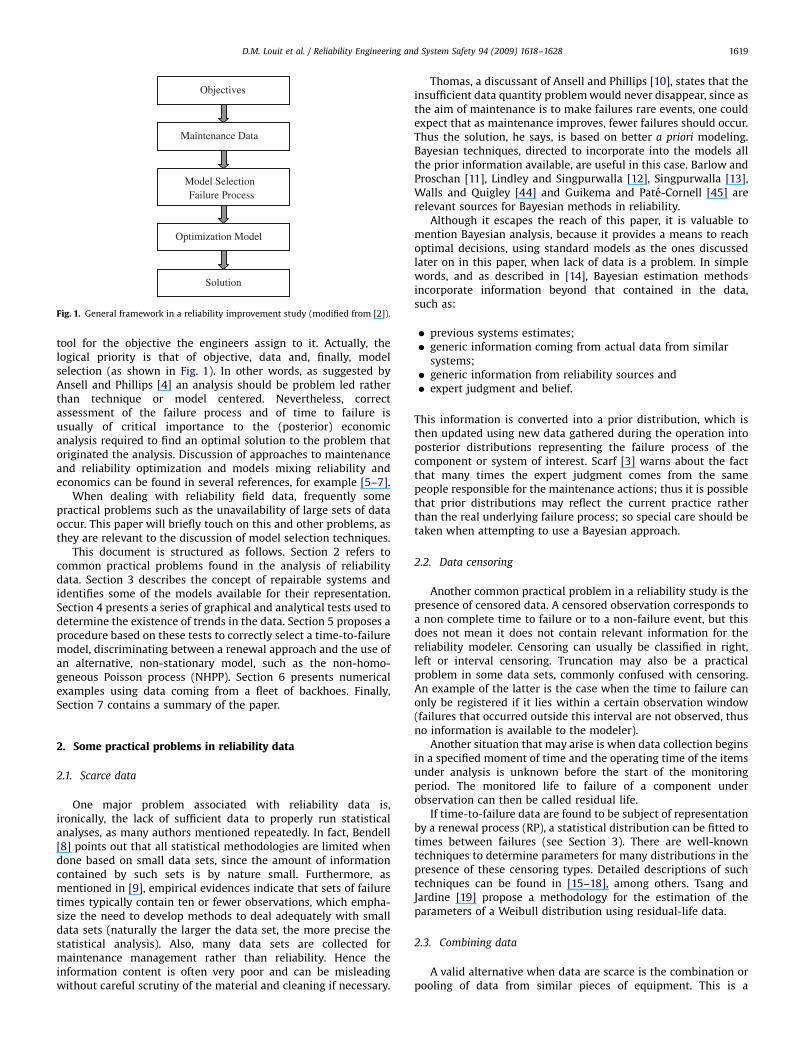
Fig. 2 shows three theoretical situations that may occur inpractice, in relation to time to failure of a particular system. Fromthe figure, it can be noticed that the three data sets generatedfrom systems A–C are very different. For A, no clear trend can be

Age

Age

Age

or each of the following diagrams, represents the occurrence of a ailure:

Fig. 2. Possible trends in time between failures.

observed from the failure data, thus an iid assumption may bemade, since time between failures is apparently independent fromthe age of the equipment. For B and C, however, a trend is clearlypresent; for B a decrease in reliability is evident, while for Creliability growth is taking place. Whenever these latter situationsoccur, and there is significant evidence for recognition of anageing process taking place, the usual RP approach has to bedisregarded, and an alternative non-stationary approach wouldusually be used to model time between failures for the system.Note that ‘‘equipment age’’ refers to the age of the system underanalysis, measured from the moment it was first put intooperation, as apposed to the time elapsed since the last repair(which is significant for a RP).

3.1. The non-homogeneous Poisson process

In practical terms, the NHPP permits the modeling of trend inthe number of failures to be found in an interval in relation to totalage of the system, through the intensity function. Two popularparameterizations for the intensity function of an NHPP are thepower law intensity (also called Weibull intensity) and the log-linear intensity.

The power law intensity gives its name to the power lawprocess (NHPP with Weibull intensity) and is given by

lðtÞ ¼ Zbtb�1, (1)

with Z, b40 and tX0.The log-linear intensity function has the form

lðtÞ ¼ eaþbt , (2)

with �Noa,boN and tX0.Several practical examples reviewed show that the power-law

process is preferred, because of its similarities with the Weibulldistribution fitting method used regularly for non-repairable data.Actually, Z is the scale parameter and b the shape parameter, andthe intensity function is of the same form of the failure rate of aWeibull distribution.

Details concerning the fitting of a power-law and log-linearintensity functions to data from water pumps in a nuclear plantare discussed in [23]. A practical example using jet engine datacombined from several pieces of equipment is found in [24].Ascher and Kobbacy [33], and Baker [34] also provide applicationsof both log-linear and power-law processes.

When using an NHPP, engineers could imagine it as a two-stage problem: the first (say, inner stage) relates to the fitting ofan intensity function to data and the second (outer stage) usesthe cumulative intensity function to estimate reliability(or probability of failure) for the system. When trends are notpresent and data can be assumed to be iid, only one stage isneeded, where directly a time-to-failure distribution is fitted todata and reliability (or probability of failure) estimates areobtained from it.

4. Trend testing techniques

Given that a clear need for trend testing in time betweenfailures data is identified, a first step in model selection should bethat of assessing the existence of trend or time dependency in thedata. Several techniques accomplish this task, and a selection ofthem is described here.

Before presenting the testing techniques, it is of greatimportance to identify the possible trends one may encounterwhen analyzing reliability data. A trend in the pattern of failurescan be monotonic or non-monotonic. In the case of a monotonictrend (such as the ones shown in Fig. 2), the system is said to be

ARTICLE IN PRESS

D.M. Louit et al. / Reliability Engineering and System Safety 94 (2009) 1618–16281622

improving (or ‘‘happy system’’) if the time between arrivals tendsto get longer (decreasing trend in number of failures); and it issaid to be deteriorating (or ‘‘sad system’’) if the times tend to getshorter (increasing trend in number of failures). Non-monotonictrends are said to occur when trends change with time or theyrepeat themselves in cycles. One common form of non-monotonictrend is the bath-tub shape trend, in which time between failuresincreases in the beginning of the equipment life, then tends to bestable for a period and decreases at the end.

It should be remembered, when testing for trend, that thechoice of the time scale could have an impact on the pattern offailures; so special attention has to be given to the selection of thetime unit (calendar hours, operating hours, production throughput, etc. [31]).

Serv

ice

life

(ith

fai

lure

)

Service life ((i-1)th failure)

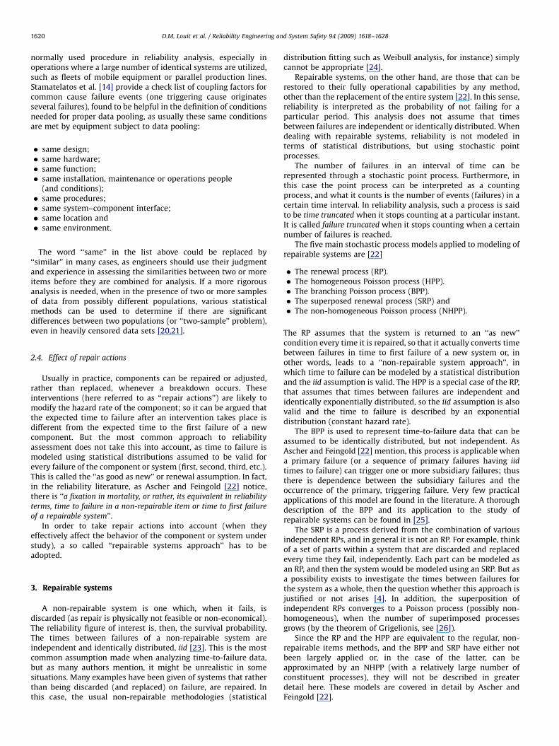
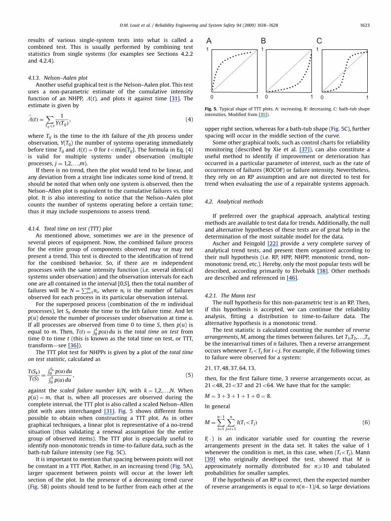
Fig. 4. Example of a successive service life plot (highlighted points indicate

anomalies).

4.1. Graphical methods

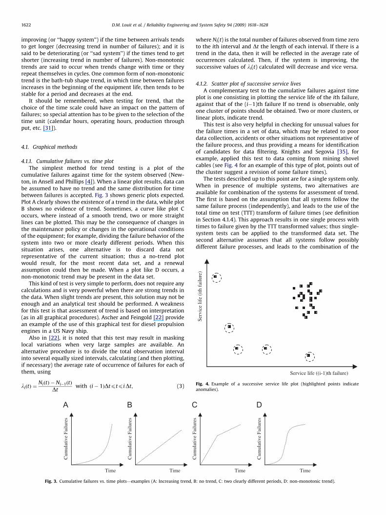
4.1.1. Cumulative failures vs. time plot

The simplest method for trend testing is a plot of thecumulative failures against time for the system observed (New-ton, in Ansell and Phillips [4]). When a linear plot results, data canbe assumed to have no trend and the same distribution for timebetween failures is accepted. Fig. 3 shows generic plots expected.Plot A clearly shows the existence of a trend in the data, while plotB shows no evidence of trend. Sometimes, a curve like plot Coccurs, where instead of a smooth trend, two or more straightlines can be plotted. This may be the consequence of changes inthe maintenance policy or changes in the operational conditionsof the equipment; for example, dividing the failure behavior of thesystem into two or more clearly different periods. When thissituation arises, one alternative is to discard data notrepresentative of the current situation; thus a no-trend plotwould result, for the most recent data set, and a renewalassumption could then be made. When a plot like D occurs, anon-monotonic trend may be present in the data set.

This kind of test is very simple to perform, does not require anycalculations and is very powerful when there are strong trends inthe data. When slight trends are present, this solution may not beenough and an analytical test should be performed. A weaknessfor this test is that assessment of trend is based on interpretation(as in all graphical procedures). Ascher and Feingold [22] providean example of the use of this graphical test for diesel propulsionengines in a US Navy ship.

Also in [22], it is noted that this test may result in maskinglocal variations when very large samples are available. Analternative procedure is to divide the total observation intervalinto several equally sized intervals, calculating (and then plotting,if necessary) the average rate of occurrence of failures for each ofthem, using

liðtÞ ¼NiðtÞ � Ni�1ðtÞ

Dtwith ði� 1ÞDtptpiDt; (3)

Time Time

Cum

ulat

ive

Failu

res

Cum

ulat

ive

Failu

res

Fig. 3. Cumulative failures vs. time plots—examples (A: Increasing trend, B

where Ni(t) is the total number of failures observed from time zeroto the ith interval and Dt the length of each interval. If there is atrend in the data, then it will be reflected in the average rate ofoccurrences calculated. Then, if the system is improving, thesuccessive values of li(t) calculated will decrease and vice versa.

4.1.2. Scatter plot of successive service lives

A complementary test to the cumulative failures against timeplot is one consisting in plotting the service life of the ith failure,against that of the (i�1)th failure If no trend is observable, onlyone cluster of points should be obtained. Two or more clusters, orlinear plots, indicate trend.

This test is also very helpful in checking for unusual values forthe failure times in a set of data, which may be related to poordata collection, accidents or other situations not representative ofthe failure process, and thus providing a means for identificationof candidates for data filtering. Knights and Segovia [35], forexample, applied this test to data coming from mining shovelcables (see Fig. 4 for an example of this type of plot, points out ofthe cluster suggest a revision of some failure times).

The tests described up to this point are for a single system only.When in presence of multiple systems, two alternatives areavailable for combination of the systems for assessment of trend.The first is based on the assumption that all systems follow thesame failure process (independently), and leads to the use of thetotal time on test (TTT) transform of failure times (see definitionin Section 4.1.4). This approach results in one single process withtimes to failure given by the TTT transformed values; thus single-system tests can be applied to the transformed data set. Thesecond alternative assumes that all systems follow possiblydifferent failure processes, and leads to the combination of the

Time Time

Cum

ulat

ive

Failu

res

Cum

ulat

ive

Failu

res

: no trend, C: two clearly different periods, D: non-monotonic trend).

ARTICLE IN PRESS

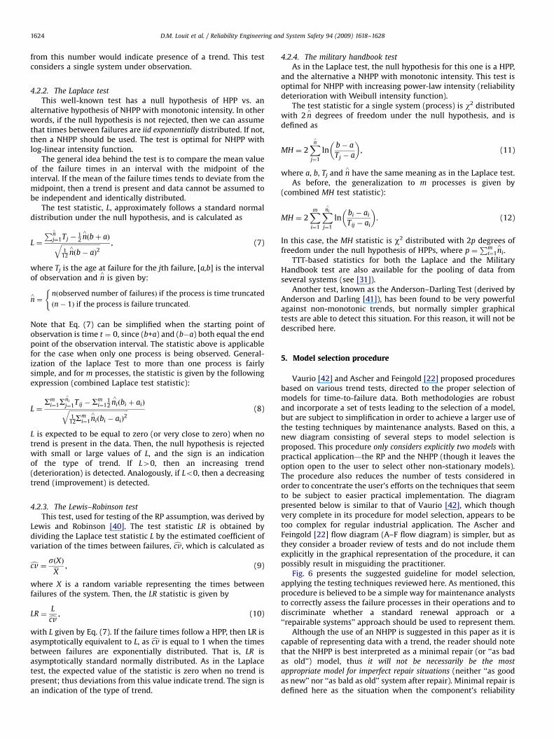
1 1 1

0 1 0 1 0 1

Fig. 5. Typical shape of TTT plots. A: increasing, B: decreasing, C: bath-tub shape

intensities. Modified from [31]).

D.M. Louit et al. / Reliability Engineering and System Safety 94 (2009) 1618–1628 1623

results of various single-system tests into what is called acombined test. This is usually performed by combining teststatistics from single systems (for examples see Sections 4.2.2and 4.2.4).

4.1.3. Nelson–Aalen plot

Another useful graphical test is the Nelson–Aalen plot. This testuses a non-parametric estimate of the cumulative intensityfunction of an NHPP, L(t), and plots it against time [31]. Theestimate is given by

L^

ðtÞ ¼XTijpt

1

YðTijÞ, (4)

where Tij is the time to the ith failure of the jth process underobservation, Y(Tij) the number of systems operating immediatelybefore time Tij and L(t) ¼ 0 for tomin{Tij}. The formula in Eq. (4)is valid for multiple systems under observation (multipleprocesses, j ¼ 1,2,y,m).

If there is no trend, then the plot would tend to be linear, andany deviation from a straight line indicates some kind of trend. Itshould be noted that when only one system is observed, then theNelson–Allen plot is equivalent to the cumulative failures vs. timeplot. It is also interesting to notice that the Nelson–Aalen plotcounts the number of systems operating before a certain time;thus it may include suspensions to assess trend.

4.1.4. Total time on test (TTT) plot

As mentioned above, sometimes we are in the presence ofseveral pieces of equipment. Now, the combined failure processfor the entire group of components observed may or may notpresent a trend. This test is directed to the identification of trendfor the combined behavior. So, if there are m independentprocesses with the same intensity function (i.e. several identicalsystems under observation) and the observation intervals for eachone are all contained in the interval [0,S], then the total number offailures will be N ¼

Pmi¼1ni, where ni is the number of failures

observed for each process in its particular observation interval.For the superposed process (combination of the m individual

processes), let Sk denote the time to the kth failure time. And letp(u) denote the number of processes under observation at time u.If all processes are observed from time 0 to time S, then p(u) isequal to m. Then, TðtÞ ¼

R t0 pðuÞdu is the total time on test from

time 0 to time t (this is known as the total time on test, or TTT,transform—see [36]).

The TTT plot test for NHPPs is given by a plot of the total time

on test statistic, calculated as

TðSkÞ

TðSÞ¼

R Sk

0 pðuÞduR S0 pðuÞdu

, (5)

against the scaled failure number k/N, with k ¼ 1,2,y,N. Whenp(u) ¼ m, that is, when all processes are observed during thecomplete interval, the TTT plot is also called a scaled Nelson–Allenplot with axes interchanged [31]. Fig. 5 shows different formspossible to obtain when constructing a TTT plot. As in othergraphical techniques, a linear plot is representative of a no-trendsituation (thus validating a renewal assumption for the entiregroup of observed items). The TTT plot is especially useful toidentify non-monotonic trends in time-to-failure data, such as thebath-tub failure intensity (see Fig. 5C).

It is important to mention that spacing between points will notbe constant in a TTT Plot. Rather, in an increasing trend (Fig. 5A),larger spacement between points will occur at the lower leftsection of the plot. In the presence of a decreasing trend curve(Fig. 5B) points should tend to be further from each other at the

upper right section, whereas for a bath-tub shape (Fig. 5C), furtherspacing will occur in the middle section of the curve.

Some other graphical tools, such as control charts for reliabilitymonitoring (described by Xie et al. [37]), can also constitute auseful method to identify if improvement or deterioration hasoccurred in a particular parameter of interest, such as the rate ofoccurrences of failures (ROCOF) or failure intensity. Nevertheless,they rely on an RP assumption and are not directed to test fortrend when evaluating the use of a repairable systems approach.

4.2. Analytical methods

If preferred over the graphical approach, analytical testingmethods are available to test data for trends. Additionally, the nulland alternative hypotheses of these tests are of great help in thedetermination of the most suitable model for the data.

Ascher and Feingold [22] provide a very complete survey ofanalytical trend tests, and present them organized according totheir null hypothesis (i.e. RP, HPP, NHPP, monotonic trend, non-monotonic trend, etc.). Hereby, only the most popular tests will bedescribed, according primarily to Elvebakk [38]. Other methodsare described and referenced in [46].

4.2.1. The Mann test

The null hypothesis for this non-parametric test is an RP. Then,if this hypothesis is accepted, we can continue the reliabilityanalysis, fitting a distribution to time-to-failure data. Thealternative hypothesis is a monotonic trend.

The test statistic is calculated counting the number of reverse

arrangements, M, among the times between failures. Let T1,T2,y,Tn

be the interarrival times of n failures. Then a reverse arrangementoccurs whenever TioTj for ioj. For example, if the following timesto failure were observed for a system:

21;17;48;37;64;13;

then, for the first failure time, 3 reverse arrangements occur, as21o48, 21o37 and 21o64. We have that for the sample:

M ¼ 3þ 3þ 1þ 1þ 0 ¼ 8.

In general

M ¼Xn�1

i¼1

Xn

j¼iþ1

IðTioTjÞ (6)

I( � ) is an indicator variable used for counting the reversearrangements present in the data set. It takes the value of 1whenever the condition is met, in this case, when (TioTj). Mann[39] who originally developed the test, showed that M isapproximately normally distributed for nX10 and tabulatedprobabilities for smaller samples.

If the hypothesis of an RP is correct, then the expected numberof reverse arrangements is equal to n(n�1)/4, so large deviations

ARTICLE IN PRESS

D.M. Louit et al. / Reliability Engineering and System Safety 94 (2009) 1618–16281624

from this number would indicate presence of a trend. This testconsiders a single system under observation.

4.2.2. The Laplace test

This well-known test has a null hypothesis of HPP vs. analternative hypothesis of NHPP with monotonic intensity. In otherwords, if the null hypothesis is not rejected, then we can assumethat times between failures are iid exponentially distributed. If not,then a NHPP should be used. The test is optimal for NHPP withlog-linear intensity function.

The general idea behind the test is to compare the mean valueof the failure times in an interval with the midpoint of theinterval. If the mean of the failure times tends to deviate from themidpoint, then a trend is present and data cannot be assumed tobe independent and identically distributed.

The test statistic, L, approximately follows a standard normaldistribution under the null hypothesis, and is calculated as

L ¼

Pn^

j¼1Tj �12 n^ðbþ aÞffiffiffiffiffiffiffiffiffiffiffiffiffiffiffiffiffiffiffiffiffiffiffiffi

112 n^ðb� aÞ2

q , (7)

where Tj is the age at failure for the jth failure, [a,b] is the intervalof observation and n

^is given by:

n^¼

nðobserved number of failuresÞ if the process is time truncated

ðn� 1Þ if the process is failure truncated:

(

Note that Eq. (7) can be simplified when the starting point ofobservation is time t ¼ 0, since (b+a) and (b�a) both equal the endpoint of the observation interval. The statistic above is applicablefor the case when only one process is being observed. General-ization of the laplace Test to more than one process is fairlysimple, and for m processes, the statistic is given by the followingexpression (combined Laplace test statistic):

L ¼Sm

i¼1Sni

^

j¼1Tij �Smi¼1

12 ni

^ðbi þ aiÞffiffiffiffiffiffiffiffiffiffiffiffiffiffiffiffiffiffiffiffiffiffiffiffiffiffiffiffiffiffiffiffiffiffiffiffiffi

112S

mi¼1n^

iðbi � aiÞ2

q (8)

L is expected to be equal to zero (or very close to zero) when notrend is present in the data. Then, the null hypothesis is rejectedwith small or large values of L, and the sign is an indicationof the type of trend. If L40, then an increasing trend(deterioration) is detected. Analogously, if Lo0, then a decreasingtrend (improvement) is detected.

4.2.3. The Lewis–Robinson test

This test, used for testing of the RP assumption, was derived byLewis and Robinson [40]. The test statistic LR is obtained bydividing the Laplace test statistic L by the estimated coefficient ofvariation of the times between failures, ccv, which is calculated as

ccv ¼sðXÞ

X, (9)

where X is a random variable representing the times betweenfailures of the system. Then, the LR statistic is given by

LR ¼Lccv

, (10)

with L given by Eq. (7). If the failure times follow a HPP, then LR isasymptotically equivalent to L, as ccv is equal to 1 when the timesbetween failures are exponentially distributed. That is, LR isasymptotically standard normally distributed. As in the Laplacetest, the expected value of the statistic is zero when no trend ispresent; thus deviations from this value indicate trend. The sign isan indication of the type of trend.

4.2.4. The military handbook test

As in the Laplace test, the null hypothesis for this one is a HPP,and the alternative a NHPP with monotonic intensity. This test isoptimal for NHPP with increasing power-law intensity (reliabilitydeterioration with Weibull intensity function).

The test statistic for a single system (process) is w2 distributedwith 2 n

^degrees of freedom under the null hypothesis, and is

defined as

MH ¼ 2Xn^

j¼1

lnb� a

Tj � a

� �, (11)

where a, b, Tj and n^

have the same meaning as in the Laplace test.As before, the generalization to m processes is given by

(combined MH test statistic):

MH ¼ 2Xmi¼1

Xni

^

j¼1

lnbi � ai

Tij � ai

� �. (12)

In this case, the MH statistic is w2 distributed with 2p degrees offreedom under the null hypothesis of HPPs, where p ¼

Pmi¼1n^

i.TTT-based statistics for both the Laplace and the Military

Handbook test are also available for the pooling of data fromseveral systems (see [31]).

Another test, known as the Anderson–Darling Test (derived byAnderson and Darling [41]), has been found to be very powerfulagainst non-monotonic trends, but normally simpler graphicaltests are able to detect this situation. For this reason, it will not bedescribed here.

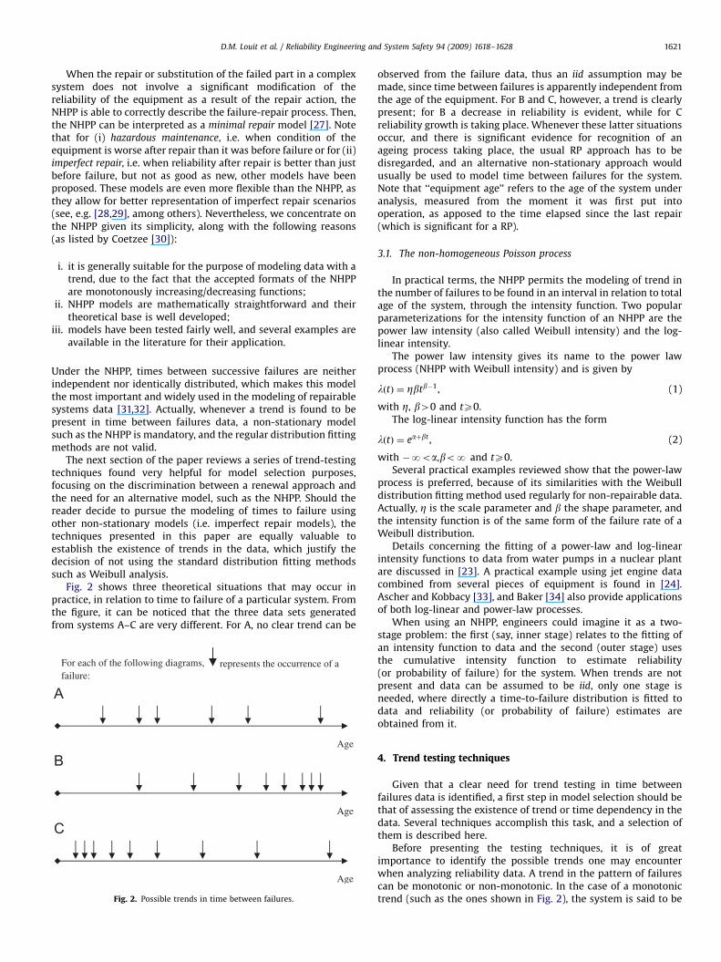
5. Model selection procedure

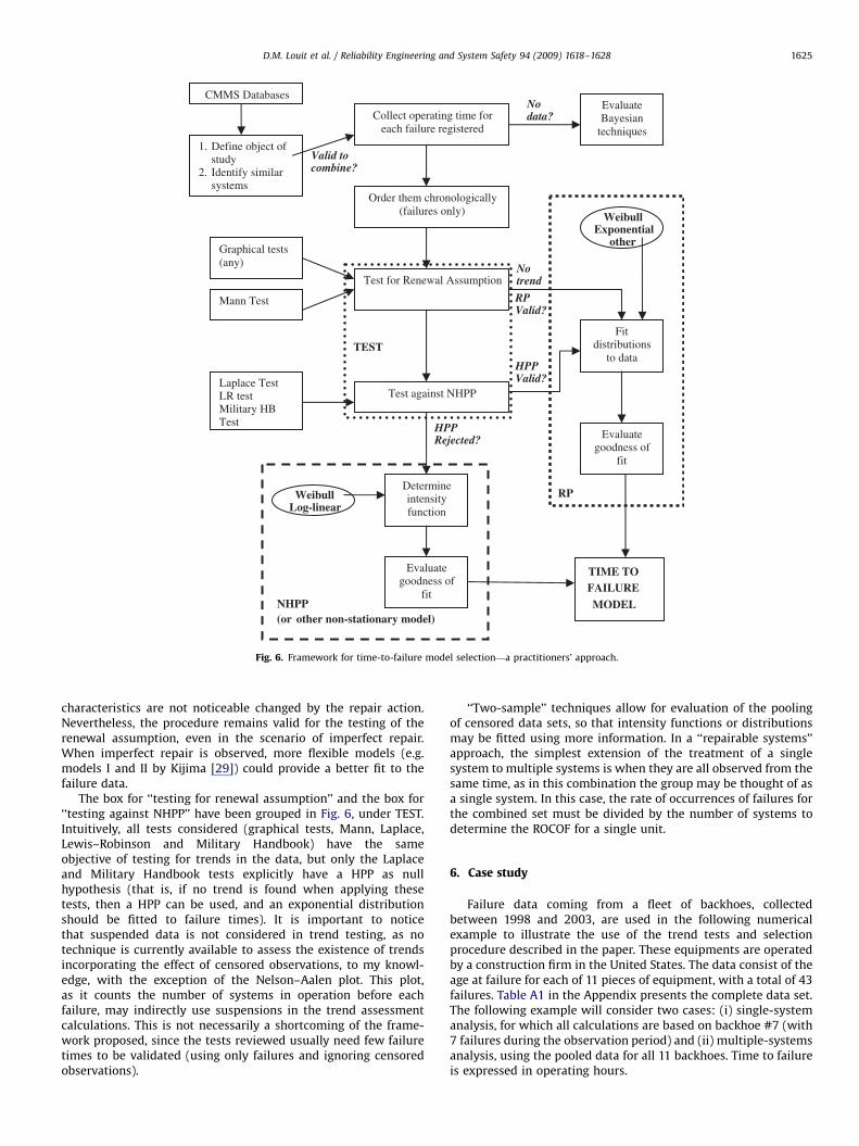
Vaurio [42] and Ascher and Feingold [22] proposed proceduresbased on various trend tests, directed to the proper selection ofmodels for time-to-failure data. Both methodologies are robustand incorporate a set of tests leading to the selection of a model,but are subject to simplification in order to achieve a larger use ofthe testing techniques by maintenance analysts. Based on this, anew diagram consisting of several steps to model selection isproposed. This procedure only considers explicitly two models withpractical application—the RP and the NHPP (though it leaves theoption open to the user to select other non-stationary models).The procedure also reduces the number of tests considered inorder to concentrate the user’s efforts on the techniques that seemto be subject to easier practical implementation. The diagrampresented below is similar to that of Vaurio [42], which thoughvery complete in its procedure for model selection, appears to betoo complex for regular industrial application. The Ascher andFeingold [22] flow diagram (A–F flow diagram) is simpler, but asthey consider a broader review of tests and do not include themexplicitly in the graphical representation of the procedure, it canpossibly result in misguiding the practitioner.

Fig. 6 presents the suggested guideline for model selection,applying the testing techniques reviewed here. As mentioned, thisprocedure is believed to be a simple way for maintenance analyststo correctly assess the failure processes in their operations and todiscriminate whether a standard renewal approach or a‘‘repairable systems’’ approach should be used to represent them.

Although the use of an NHPP is suggested in this paper as it iscapable of representing data with a trend, the reader should notethat the NHPP is best interpreted as a minimal repair (or ‘‘as badas old’’) model, thus it will not be necessarily be the most

appropriate model for imperfect repair situations (neither ‘‘as goodas new’’ nor ‘‘as bald as old’’ system after repair). Minimal repair isdefined here as the situation when the component’s reliability

ARTICLE IN PRESS

Collect operating time for each failure registered

Order them chronologically (failures only)

Test for Renewal Assumption

Evaluate Bayesian

techniques

CMMS Databases

1. Define object of study

2. Identify similar systems

Nodata?

Valid to combine?

Fitdistributions

to data

Notrend

RPValid?

Evaluate goodness of

fit

Graphical tests (any)

Mann Test

Test against NHPP Laplace Test LR test Military HB Test

HPPValid?

Weibull Exponential

other

HPPRejected?

Determine intensityfunction

Weibull Log-linear

Evaluate goodness of

fit

RP

NHPP(or other non-stationary model)

TIME TO FAILUREMODEL

TEST

Fig. 6. Framework for time-to-failure model selection—a practitioners’ approach.

D.M. Louit et al. / Reliability Engineering and System Safety 94 (2009) 1618–1628 1625

characteristics are not noticeable changed by the repair action.Nevertheless, the procedure remains valid for the testing of therenewal assumption, even in the scenario of imperfect repair.When imperfect repair is observed, more flexible models (e.g.models I and II by Kijima [29]) could provide a better fit to thefailure data.

The box for ‘‘testing for renewal assumption’’ and the box for‘‘testing against NHPP’’ have been grouped in Fig. 6, under TEST.Intuitively, all tests considered (graphical tests, Mann, Laplace,Lewis–Robinson and Military Handbook) have the sameobjective of testing for trends in the data, but only the Laplaceand Military Handbook tests explicitly have a HPP as nullhypothesis (that is, if no trend is found when applying thesetests, then a HPP can be used, and an exponential distributionshould be fitted to failure times). It is important to noticethat suspended data is not considered in trend testing, as notechnique is currently available to assess the existence of trendsincorporating the effect of censored observations, to my knowl-edge, with the exception of the Nelson–Aalen plot. This plot,as it counts the number of systems in operation before eachfailure, may indirectly use suspensions in the trend assessmentcalculations. This is not necessarily a shortcoming of the frame-work proposed, since the tests reviewed usually need few failuretimes to be validated (using only failures and ignoring censoredobservations).

‘‘Two-sample’’ techniques allow for evaluation of the poolingof censored data sets, so that intensity functions or distributionsmay be fitted using more information. In a ‘‘repairable systems’’approach, the simplest extension of the treatment of a singlesystem to multiple systems is when they are all observed from thesame time, as in this combination the group may be thought of asa single system. In this case, the rate of occurrences of failures forthe combined set must be divided by the number of systems todetermine the ROCOF for a single unit.

6. Case study

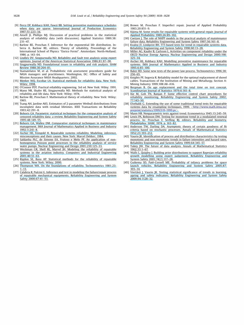
Failure data coming from a fleet of backhoes, collectedbetween 1998 and 2003, are used in the following numericalexample to illustrate the use of the trend tests and selectionprocedure described in the paper. These equipments are operatedby a construction firm in the United States. The data consist of theage at failure for each of 11 pieces of equipment, with a total of 43failures. Table A1 in the Appendix presents the complete data set.The following example will consider two cases: (i) single-systemanalysis, for which all calculations are based on backhoe #7 (with7 failures during the observation period) and (ii) multiple-systemsanalysis, using the pooled data for all 11 backhoes. Time to failureis expressed in operating hours.

ARTICLE IN PRESS

D.M. Louit et al. / Reliability Engineering and System Safety 94 (2009) 1618–16281626

6.1. Single-system example

Backhoe number 7 had seven failures during the years1998–2003. The times between failures are: 3090, 850, 904, 166,395, 242 and 496 h. By looking at these numbers, deteriorationappears to be present in the data, that is, times between failuresseem to be shorter as the equipment ages. Fig. 7 (cumulativefailures vs. time plot) confirms this belief. Similar plots areobtained for 7 out of the 11 backhoes analyzed. When plotting thesuccessive service lives, only two points lay outside the maincluster (implying that one failure time might be an anomaly, seeFig. 8). This is the first service life of 3090 hours, which is muchlarger than the rest. This failure time (as well as all other failuretimes in the data set) was validated by the fleet operator;thus noneed for further revision or elimination of data is identified.According to the procedure depicted in Fig. 6, the Mann test couldbe used to confirm the findings obtained by the cumulativefailures vs. time plot, that a trend is present in the data. In thisexample, M ¼ 0+1+0+3+1+1 ¼ 6. This number differs significantlyfrom the expected value of 10.5. Actually, it is significantly low, asPðMoM=H1Þ ¼ 0:881, implying that the data show a degradationtrend (H1 is the alternative hypothesis, of degradation trend).

As a trend was identified, a renewal approach is not valid formodeling time to failure, and a ‘‘repairable systems’’ approach isrequired. Alternatively, testing through parametric tests such asthe Laplace, Lewis–Robinson or Military Handbook tests wasperformed, with similar results (NHPP with monotonic intensity isthe model selected). The Laplace statistic L equals 2.189 forbackhoe #7. This is given that the process in this case is failuretruncated (e.g. final point of the observation interval given by thefailure time of the last recorded failure event). This result is

0

1

2

3

4

5

6

7

8

0

Age (hours)

Cum

ulat

ive

failu

res

1000 2000 3000 4000 5000 6000 7000

Fig. 7. Cumulative failures vs. time plot—backhoe #7.

0

500

1000

1500

2000

2500

3000

3500

0

Serv

ice

life

(ith

fai

lure

) (h

ours

)

500 1000 1500 2000 2500 3000 3500

Service life ((i-1)th failure) (hours)

Fig. 8. Successive service life plot—backhoe #7.

statistically significant (at 0.05 significance level), indicating anincreasing trend in the intensity of the failure process (i.e.degradation). The LR statistic equals 10.187 and the MH statisticequals 3.5698, leading us to the same conclusion (the latter at 0.01significance level). Fitting of an intensity function to the data isthe next step considered in the procedure presented in Fig. 6, butwill not be included here for brevity. It is important to mentionthat not all tests need be performed in this case. On the contrary,the idea is to choose a test that accommodates the user and, onlyin the case that not enough evidence is available, then validate itsresults using a second testing technique.

6.2. Multiple-system example

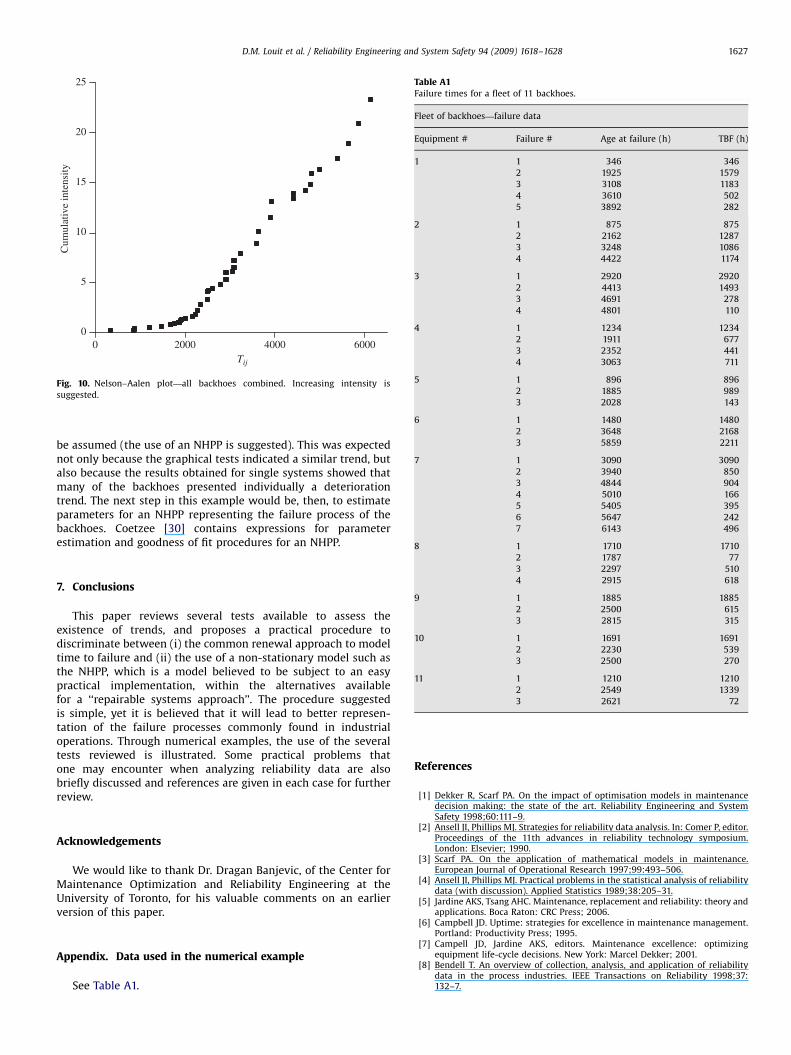
If we were interested in modeling the time to failure for thepooled group of backhoes, existence of trends in the pooledbehavior should be assessed. A common mistake is to assume thatevery piece of equipment operated for the same number of hoursover the entire interval, which in this case is not true. As thesebackhoes are operated by a construction company in differentprojects, during the same observation period of 1998–2003, someof them operated more than 6000 h, whereas others barelyreached 2500 h of operation. Then, for the performance ofgraphical tests such as the TTT or Nelson–Aalen plots, the modelershould have special care in identifying the number of units inoperation for different ages of the fleet. Note that time isexpressed in operating hours, so in the superposed failure process,11 backhoes can be considered to be ‘‘in operation’’ just for theinterval between t ¼ 0 and t ¼ 2028 operating hours. For moreadvanced ages of the fleet, the number of backhoes in operationdecreases. Fig. 9 shows a TTT plot constructed for this example.From the form of the curve, a clear indication of an increasingtrend in the intensity of failures is observed (i.e. degradation).Fig. 10 presents a Nelson-Aalen plot for the same data, againsuggesting the same conclusion.

Results for the combined Laplace and Military Handbook testsare the following: L ¼ 3.096 (significant indicator of degradation,at 0.01 significance level) and MH ¼ 31.859 (significant indicatorof degradation, at 0.01 significance level). Then, the pooled failurebehavior for the fleet effectively presents a trend, thus a RP cannot

0

1

10

Scaled failure number

TT

T s

tatis

tic

Fig. 9. TTT plot—all backhoes combined. Increasing intensity is suggested.

ARTICLE IN PRESS

0

5

10

15

20

25

0

Cum

ulat

ive

inte

nsity

2000 4000 6000Tij

Fig. 10. Nelson–Aalen plot—all backhoes combined. Increasing intensity is

suggested.

Table A1Failure times for a fleet of 11 backhoes.

Fleet of backhoes—failure data

Equipment # Failure # Age at failure (h) TBF (h)

1 1 346 346

2 1925 1579

3 3108 1183

4 3610 502

5 3892 282

2 1 875 875

2 2162 1287

3 3248 1086

4 4422 1174

3 1 2920 2920

2 4413 1493

3 4691 278

4 4801 110

4 1 1234 1234

2 1911 677

3 2352 441

4 3063 711

5 1 896 896

2 1885 989

3 2028 143

6 1 1480 1480

2 3648 2168

3 5859 2211

7 1 3090 3090

2 3940 850

3 4844 904

4 5010 166

5 5405 395

6 5647 242

7 6143 496

8 1 1710 1710

D.M. Louit et al. / Reliability Engineering and System Safety 94 (2009) 1618–1628 1627

be assumed (the use of an NHPP is suggested). This was expectednot only because the graphical tests indicated a similar trend, butalso because the results obtained for single systems showed thatmany of the backhoes presented individually a deteriorationtrend. The next step in this example would be, then, to estimateparameters for an NHPP representing the failure process of thebackhoes. Coetzee [30] contains expressions for parameterestimation and goodness of fit procedures for an NHPP.

2 1787 77

3 2297 510

4 2915 618

9 1 1885 1885

2 2500 615

3 2815 315

10 1 1691 1691

2 2230 539

3 2500 270

11 1 1210 1210

2 2549 1339

3 2621 72

7. Conclusions

This paper reviews several tests available to assess theexistence of trends, and proposes a practical procedure todiscriminate between (i) the common renewal approach to modeltime to failure and (ii) the use of a non-stationary model such asthe NHPP, which is a model believed to be subject to an easypractical implementation, within the alternatives availablefor a ‘‘repairable systems approach’’. The procedure suggestedis simple, yet it is believed that it will lead to better represen-tation of the failure processes commonly found in industrialoperations. Through numerical examples, the use of the severaltests reviewed is illustrated. Some practical problems thatone may encounter when analyzing reliability data are alsobriefly discussed and references are given in each case for furtherreview.

Acknowledgements

We would like to thank Dr. Dragan Banjevic, of the Center forMaintenance Optimization and Reliability Engineering at theUniversity of Toronto, for his valuable comments on an earlierversion of this paper.

Appendix. Data used in the numerical example

See Table A1.

References

[1] Dekker R, Scarf PA. On the impact of optimisation models in maintenancedecision making: the state of the art. Reliability Engineering and SystemSafety 1998;60:111–9.

[2] Ansell JI, Phillips MJ. Strategies for reliability data analysis. In: Comer P, editor.Proceedings of the 11th advances in reliability technology symposium.London: Elsevier; 1990.

[3] Scarf PA. On the application of mathematical models in maintenance.European Journal of Operational Research 1997;99:493–506.

[4] Ansell JI, Phillips MJ. Practical problems in the statistical analysis of reliabilitydata (with discussion). Applied Statistics 1989;38:205–31.

[5] Jardine AKS, Tsang AHC. Maintenance, replacement and reliability: theory andapplications. Boca Raton: CRC Press; 2006.

[6] Campbell JD. Uptime: strategies for excellence in maintenance management.Portland: Productivity Press; 1995.

[7] Campell JD, Jardine AKS, editors. Maintenance excellence: optimizingequipment life-cycle decisions. New York: Marcel Dekker; 2001.

[8] Bendell T. An overview of collection, analysis, and application of reliabilitydata in the process industries. IEEE Transactions on Reliability 1998;37:132–7.

ARTICLE IN PRESS

D.M. Louit et al. / Reliability Engineering and System Safety 94 (2009) 1618–16281628

[9] Percy DF, Kobbacy KAH, Fawzi BB. Setting preventive maintenance scheduleswhen data are sparse. International Journal of Production Economics1997;51:223–34.

[10] Ansell JI, Phillips MJ. Discussion of practical problems in the statisticalanalysis of reliability data (with discussion). Applied Statistics 1989;38:231–47.

[11] Barlow RE, Proschan F. Inference for the exponential life distribution. In:Serra A, Barlow RE, editors. Theory of reliability, Proceedings of theInternational School of Physics ‘‘Enrico Fermi’’. Amsterdam: North-Holland;1986. p. 143–64.

[12] Lindley DV, Singpurwalla ND. Reliability and fault tree analysis using expertopinions. Journal of the American Statistical Association 1986;81:87–90.

[13] Singpurwalla ND. Foundational issues in reliability and risk analysis. SIAMReview 1988;30:264–81.

[14] Stamatelatos M, et al. Probabilistic risk assessment procedures guide forNASA managers and practitioners. Washington, DC: Office of Safety andMission Assurance NASA Headquarters; 2002.

[15] Meeker WQ, Escobar LA. Statistical methods for reliability data. New York:Wiley; 1998.

[16] O’Connor PDT. Practical reliability engineering. 3rd ed. New York: Wiley; 1991.[17] Mann NR, Shafer RE, Singpurwalla ND. Methods for statistical analysis of

reliability and life data. New York: Wiley; 1974.[18] Barlow RE, Proschan F. Mathematical theory of reliability. New York: Wiley;

1965.[19] Tsang AH, Jardine AKS. Estimators of 2-parameter Weibull distributions from

incomplete data with residual lifetimes. IEEE Transactions on Reliability1993;42:291–8.

[20] Bohoris GA. Parametric statistical techniques for the comparative analysis ofcensored reliability data: a review. Reliability Engineering and System Safety1995;48:149–55.

[21] Bohoris GA, Walley DM. Comparative statistical techniques in maintenancemanagement. IMA Journal of Mathematics Applied in Business and Industry1992;3:241–8.

[22] Ascher HE, Feingold H. Repairable systems reliability. Modeling, inference,misconceptions and their causes. New York: Marcel Dekker; 1984.

[23] Saldanha PLC, de Simone EA, Frutoso e Melo PF. An application of non-homogeneus Poisson point processes to the reliability analysis of servicewater pumps. Nuclear Engineering and Design 2001;210:125–33.

[24] Weckman GR, Shell RL, Marvel JH. Modeling the reliability of repairablesystems in the aviation industry. Computers and Industrial Engineering2001;40:51–63.

[25] Rigdon SE, Basu AP. Statistical methods for the reliability of repairablesystems. New York: Wiley; 2000.

[26] Thompson WA. On the foundations of reliability. Technometrics 1981;23:1–13.

[27] Calabria R, Pulcini G. Inference and test in modeling the failure/repair processof repairable mechanical equipments. Reliability Engineering and SystemSafety 2000;67:41–53.

[28] Brown M, Proschan F. Imperfect repair. Journal of Applied Probability1983;20:851–9.

[29] Kijima M. Some results for repairable systems with general repair. Journal ofApplied Probability 1989;26:89–102.

[30] Coetzee J. The role of NHPP models in the practical analysis of maintenancefailure data. Reliability Engineering and System Safety 1997;56:161–8.

[31] Kvaloy JT, Lindqvist BH. TTT-based tests for trend in repairable systems data.Reliability Engineering and System Safety 1998;60:13–28.

[32] Miller AG, Kaufer B, Carlsson L. Activities on component reliability under theOECD Nuclear Energy Agency. Nuclear Engineering and Design 2000;198:325–34.

[33] Ascher HE, Kobbacy KAH. Modelling preventive maintenance for repairablesystems. IMA Journal of Mathematics Applied in Business and Industry1995;6:85–100.

[34] Baker RD. Some new tests of the power law process. Technometrics 1996;38:256–65.

[35] Knights PF, Segovia R. Reliability model for the optimal replacement of shovelcables. Transactions of the Institution of Mining and Metallurgy, Section A:Mining Industry 1999;108:A8–A16.

[36] Bergman B. On age replacement and the total time on test concept.Scandinavian Journal of Statistics 1979;6:161–8.

[37] Xie M, Goh TN, Ranjan P. Some effective control chart procedures forreliability monitoring. Reliability Engineering and System Safety 2002;77:143–50.

[38] Elvebakk G. Extending the use of some traditional trend tests for repairablesystems data by resampling techniques, 1999. /http://www.math.ntnu.no/preprint/statistics/1999/S19-1999.psS.

[39] Mann HB. Nonparametric tests against trend. Econometrica 1945;13:245–59.[40] Lewis PA, Robinson DW. Testing for monotone trend in a modulated renewal

process. In: Proschan F, Serfling RJ, editors. Reliability and biometry.Philadelphia: SIAM; 1974. p. 163–82.

[41] Anderson TW, Darling DA. Asymptotic theory of certain goodness of fitcriteria based on stochastic processes. Annals of Mathematical Statistics1952;23:193–212.

[42] Vaurio JK. Identification of process and distribution characteristics by testingmonotonic and non-monotonic trends in failure intensities and hazard rates.Reliability Engineering and System Safety 1999;64:345–57.

[43] Tukey JW. The future of data analysis. Annals of Mathematical Statistics1962;33:1–67.

[44] Walls L, Quigley J. Building prior distributions to support Bayesian reliabilitygrowth modelling using expert judgement. Reliability Engineering andSystem Safety 2001;74(2):117–28.

[45] Guikema SD, Pate-Cornell ME. Probability of infancy problems for spacelaunch vehicles. Reliability Engineering and System Safety 2005;87:303–14.

[46] Viertava J, Vaurio JK. Testing statistical significance of trends in learning,ageing and safety indicators. Reliability Engineering and System Safety2009;94:1128–32.