Discrete Optimization

A polynomial algorithm for 2-degree cyclic robot scheduling

Ada Che a, Chengbin Chu a,*, Eugene Levner b

a Laboratoire LOSI, Universit�ee de Technologie de Troyes, 12 Rue Marie Curie - BP 2060, 10010 Troyes Cedex, Franceb Centre for Technological Education, 52 Golomb Street, Holon 58102, Israel

Received 30 November 1999; accepted 7 November 2000

Abstract

This paper studies the 2-degree cyclic scheduling of identical parts in a no-wait robotic flow shop where exactly two

parts enter and leave the production line in a cycle. The objective is to minimize the cycle time. We propose a polynomial

algorithm to find an optimal 2-degree cyclic schedule of robot moves. The algorithm can be implemented in OðN 8 logNÞwhere N is the number of machines in the considered robotic cell. The proposed algorithm is also extended to problems

where the two parts are not identical. Computational results is presented to test and evaluate the proposed algorithm.

� 2002 Elsevier Science B.V. All rights reserved.

Keywords: Cyclic scheduling; Transporting robot; Cycle time minimization; Complexity

1. Introduction

This paper studies the 2-degree cyclic scheduling of identical parts in a no-wait robotic flow shop where

two parts enter and leave the production line in a cycle. Such a production cell has two types of resources:machines and one material handling robot or hoist. The robot is programmed to perform a fixed sequence

of moves repeatedly. Each repetition of the sequence is called a cycle.

Cyclic scheduling has received much attention from researchers and a lot of work has been published,

due to the applicability of such studies. This environment corresponds to mass production industry. In such

an industry, production lines are specially designed to produce very few specific types of parts with very

large lot size and therefore can be approximated by cyclic production model.

On the other hand, industrial robots or other material handling tools play a more and more important

role in manufacturing systems. They are in charge of transporting parts from one machine to another forthe next operation. The productivity of such production lines largely depends on the schedule of the robot

activities, especially when the intermediate storage area is limited in order to limit the work-in-process.

This is particularly the case in PCB electroplating process and other galvanization processes. In such a

production line, a part must be successively soaked in chemical tanks during a specified period of time. The

European Journal of Operational Research 145 (2003) 31–44

www.elsevier.com/locate/dsw

*Corresponding author. Tel.: +33-3-25-71-56-30; fax: +33-3-25-71-56-49.

E-mail address: chengbin.chu@univ-troyes.fr (C. Chu).

0377-2217/03/$ - see front matter � 2002 Elsevier Science B.V. All rights reserved.

PII: S0377-2217 (02 )00175-3

transport of parts from a tank to another is carried out by a robot or a hoist. Due to the specificity of

chemical process, parts are not allowed to be stored. Instead, they must be immediately removed from a

tank and transported to the next tank, as soon as the operation is completed.

Cyclic schedules can be distinguished according to the number of parts introduced into the system in a

cycle. In an n-degree cyclic schedule, also called n-cycle schedule, n (nP 1) parts are introduced during each

cycle; that is, exactly n parts are transported to and removed from each machine during a cycle. Thethroughput of an n-degree cyclic schedule is defined as n divided by the whole cycle length called cycle time.

Many researchers have studied simple cycle schedules [1–6]; i.e., 1-degree cyclic schedules. In practice,

however, simple cycle schedules are not necessarily optimal. In general, n-degree cyclic schedules with n > 1would have larger throughput. Lei and Wang [3], Song et al. [5] noticed that a 2-degree cyclic schedule may

be better than an optimal simple cycle schedule, which is also confirmed in our experiments. Therefore, it is

relevant to study multiple-degree cyclic schedules, on which little work has been done. This paper can be

considered as a preliminary work in this direction. Lei and Wang [3] presented a branch-and-bound al-

gorithm to generate an optimal 2-degree cyclic schedule with time window constraints. Song et al. [5]developed a mixed integer linear programming model for scheduling a chemical processing tank line with

constant processing times, and proposed a heuristic where the simple cycle assumption is relaxed. Levner

et al. [7] proposed a geometric algorithm to find a 2-degree cyclic schedule with constant processing times

in a nowait robotic flow shop. They conjectured that the problem was polynomially solvable. However,

they failed to prove or disprove it theoretically. Kats et al. [8] developed an algorithm based on a sieve

method for multiple-degree cyclic scheduling with constant processing times. But their method is restricted

to solving scheduling problems with integer input data and seeking for an integer cycle time. Therefore, it

cannot guarantee the optimality of the obtained solution, even for scheduling problems with integer inputdata as required, since, as shown in this paper (see Section 6), the optimal cycle time may not be integer

even with integer input data.

This paper proposes a polynomial algorithm to find an optimal 2-degree cyclic schedule with constant

processing times in a no-wait robotic flow shop. This algorithm can be implemented in OðN 8 logNÞ where Nis the number of machines in the considered robotic cell. The proposed algorithm is also extended to solve

cyclic scheduling problems where the two parts introduced in a cycle are not identical. The basic idea of the

paper is to use prohibited intervals for decision variables. This idea was also used in [7,9].

This paper is organized as follows. The 2-degree cyclic scheduling problem with constant processingtimes is formulated in Section 2. Section 3 proposes an algorithm to find an optimal solution. The com-

plexity of the algorithm is analyzed in Section 4. Section 5 extends the proposed algorithm to problems

where the two parts introduced in a cycle are not identical. Section 6 gives computational results and

Section 7 concludes the paper.

2. Problem formulation

Consider a robotic cell composed of N machines, M1; . . . ;MN , a loading station M0 and an unloading

station MNþ1. A single type of part is processed in such a robotic cell. After a part is removed from M0, it is

processed through machines M1;M2; . . . ;MN , and finally leaves the system from MNþ1. A robot or hoist is

responsible for moving parts from a machine to the next one. For simplicity, let mi ði ¼ 0; 1; . . . ;NÞ denotesthe robot activity of moving a part from Mi to Miþ1. The time required for the robot to perform move mi,

denoted as hi, 06 i6N , is known. So is the time for the robot to travel from Mi to Mj ð06 i; j6N þ 1Þwithout transporting parts (such a travel is called void move). This latter time is denoted as ri;j. Machine Mi,

16 i6N , can process at most one part at a time. The processing time on each machine is a known constant,denoted by ti, 06 i6N . As soon as an operation is completed on a machine, the part must be removed fromthis machine and transferred to the next one without any delay. Such a system is called no-wait system.

32 A. Che et al. / European Journal of Operational Research 145 (2003) 31–44

The robot is programmed to perform a fixed sequence of moves repeatedly. Each repetition of the se-

quence of moves is called a cycle. The duration of a cycle is called cycle time, denoted by T. The sequence of

moves performed by the robot in each cycle is represented by a cyclic schedule.

As mentioned in the introduction, this paper deals with 2-degree cyclic schedules; that is, exactly two

parts enter and leave the system in a cycle. For each machine, during a cycle, exactly two parts arrive at the

machine and exactly two parts are removed from it. Parts are introduced into the production line one afteranother respectively at time instant 0; T1; T ; T þ T1; 2T ; 2T þ T1; . . ., where T > T1 > 0. For the sake ofclarity, in this paper, the parts introduced at time 0; T ; 2T ; . . ., are called A-parts A0;A1;A2; . . ., while thoseentering at time T1; T þ T1; 2T þ T1; . . ., are called B-parts B0;B1;B2; . . . The ith move ði ¼ 0; 1; . . . ; 2N þ 1Þperformed by the robot in a cycle is denoted as m½i�.

In the following, we make the following assumptions commonly known as triangle inequality, which also

corresponds to what happens in practice:

hj P rj;jþ1; j ¼ 0; 1; 2; . . . ;N ;

ri;j 6 ri;k þ rk;j; i; j; k ¼ 0; 1; 2; . . . ;N þ 1:

The first relation means that a travel between two machines while transporting a part takes more time

than the same travel but without transporting part. The second relation means that a direct travel takes less

time than passing by an intermediate point.

A schedule is feasible if and only if it satisfies the following three constraints:

• The part processing time constraints. The time that a part spends on machine Mi is exactly ti, i ¼1; 2; . . . ;N .

• The machine capacity constraints. Machine Mi, i ¼ 1; 2; . . . ;N , must be empty when a part arrives at Mi.

• The robot capacity constraints. For any i ¼ 0; 1; . . . ; 2N þ 1, after the robot finishes a move m½i�, there

must be sufficient time for the robot to travel from machine M½i�þ1, to which it just finished transporting

a part, to machine M½iþ1�, from which the robot must transport the next part.

2.1. Formulation of machine capacity constraints

The machine capacity constraints mean that when a part arrives at a machine, the previous part has been

removed from that machine, since each machine can process at most one part at a time. Considering a

production line in steady state, it must be guaranteed that (a) when a B-part arrives at a machine, the

previous A-part processed by the same machine be moved out; (b) when an A-part arrives at a machine, the

previous B-part be removed from that machine.Let Zj denote the completion time of the jth operation of part A0. We have

Zj ¼Xj

i¼1ðhi�1 þ tiÞ; j ¼ 0; 1; . . . ;N : ð1Þ

In order to simplify the notation, we define

fi;j ¼ Zi þ hi þ riþ1;j � Zj; i; j ¼ 0; 1; 2; . . .N :

Due to constraint (a), for any machine Mj, j ¼ 1; 2; . . . ;N , part A0 must be removed from Mj before part

B0 arrives. Since there is only one robot, it must remove part A0 from Mj, transport it to Mjþ1 and then

transport part B0 (from machine Mj�1) to Mj. It is known that part A0 is removed from Mj at time Zj and

arrives at Mjþ1 at time Zj þ hj, and the transportation of part B0 (from machine Mj�1) to Mj starts at

Zj�1 þ T1. This requirement can be formulated as

A. Che et al. / European Journal of Operational Research 145 (2003) 31–44 33

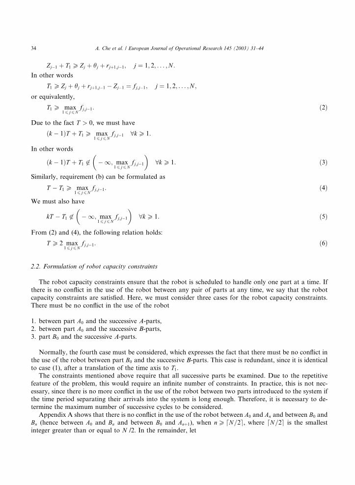
Zj�1 þ T1 P Zj þ hj þ rjþ1;j�1; j ¼ 1; 2; . . . ;N :

In other words

T1 P Zj þ hj þ rjþ1;j�1 � Zj�1 ¼ fj;j�1; j ¼ 1; 2; . . . ;N ;

or equivalently,

T1 P max16 j6N

fj;j�1: ð2Þ

Due to the fact T > 0, we must have

ðk � 1ÞT þ T1 P max16 j6N

fj;j�1 8kP 1:

In other words

ðk � 1ÞT þ T1 62��1; max

16 j6Nfj;j�1

�8k P 1: ð3Þ

Similarly, requirement (b) can be formulated as

T � T1 P max16 j6N

fj;j�1: ð4Þ

We must also have

kT � T1 62��1; max

16 j6Nfj;j�1

�8kP 1: ð5Þ

From (2) and (4), the following relation holds:

T P 2 max16 j6N

fj;j�1: ð6Þ

2.2. Formulation of robot capacity constraints

The robot capacity constraints ensure that the robot is scheduled to handle only one part at a time. If

there is no conflict in the use of the robot between any pair of parts at any time, we say that the robot

capacity constraints are satisfied. Here, we must consider three cases for the robot capacity constraints.

There must be no conflict in the use of the robot

1. between part A0 and the successive A-parts,2. between part A0 and the successive B-parts,3. part B0 and the successive A-parts.

Normally, the fourth case must be considered, which expresses the fact that there must be no conflict in

the use of the robot between part B0 and the successive B-parts. This case is redundant, since it is identicalto case (1), after a translation of the time axis to T1.The constraints mentioned above require that all successive parts be examined. Due to the repetitive

feature of the problem, this would require an infinite number of constraints. In practice, this is not nec-

essary, since there is no more conflict in the use of the robot between two parts introduced to the system if

the time period separating their arrivals into the system is long enough. Therefore, it is necessary to de-

termine the maximum number of successive cycles to be considered.

Appendix A shows that there is no conflict in the use of the robot between A0 and An and between B0 andBn (hence between A0 and Bn and between B0 and Anþ1), when nP N=2d e, where N=2d e is the smallestinteger greater than or equal to N /2. In the remainder, let

34 A. Che et al. / European Journal of Operational Research 145 (2003) 31–44

n� ¼ N=2d e: ð7ÞNow come back to the formulation of the robot capacity constraints. Constraints (1) require that for any

k, k ¼ 1; 2; . . . ; n� � 1, for any j, j ¼ 0; 1; . . . ;N � 2, and for any i, i ¼ jþ 2; . . . ;N , the transport of part A0from Mi to Miþ1 be done either before or after part Ak is moved from Mj to Mjþ1.

1 Knowing that the

transport of part A0 (respectively Ak) from Mi (respectively Mj) to Miþ1 (respectively Mjþ1) starts at Zi

(respectively Zj þ kT ) and is completed at Zi þ hi (respectively Zj þ kT þ hj), we must have:

either Zi P Zj þ kT þ hj þ rjþ1;ior Zj þ kT P Zi þ hi þ riþ1;jfor any j ¼ 0; 1; . . . ;N � 2; i ¼ jþ 2; . . . ;N and k ¼ 1; 2; . . . ; n� � 1.That is

either kT 6Zi � Zj � hj � rjþ1;i ¼ �fj;ior kT P Zi � Zj þ hi þ riþ1;j ¼ fi;jfor any j ¼ 0; 1; . . . ;N � 2, i ¼ jþ 2; . . . ;N and k ¼ 1; 2; . . . ; n� � 1.In other words,

kT 62[N�2

j¼0

[Ni¼jþ2

ð�fj;i; fi;jÞ; k ¼ 1; 2; . . . ; n� � 1: ð8Þ

Similarly, according to constraints (2), we obtain

ðk � 1ÞT þ T1 62[N�2

j¼0

[Ni¼jþ2

ð�fj;i; fi;jÞ; k ¼ 1; 2; . . . ; n�: ð9Þ

According to constraints (3), we have

kT � T1 62[N�2

j¼0

[Ni¼jþ2

ð�fj;i; fi;jÞ; k ¼ 1; 2; . . . ; n�: ð10Þ

According to (3), (5), (6) and (8)–(10), the 2-degree cyclic scheduling problems with constant processing

times can be formulated as follows, with T and T1 as decision variables:

Minimize T ð11Þ

subject to kT 62 I 0 ¼ I [��1; 2 max

16 j6Nfj;j�1

�; k ¼ 1; 2; . . . ; n� � 1; ð12Þ

ðk � 1ÞT þ T1 62 I 00 ¼ I [��1; max

16 j6Nfj;j�1

�; k ¼ 1; 2; . . . ; n�; ð13Þ

kT � T1 62 I 00; k ¼ 1; 2; . . . ; n�; ð14Þ

where

I ¼[N�2

j¼0

[Ni¼jþ2

�� fj;i; fi;j

�: ð15Þ

1 The case i ¼ jþ 1 is not considered here since the tank capacity constraints already require that the transport of part A0 fromMjþ1to Mjþ2 be done before part Ak is moved from Mj to Mjþ1.

A. Che et al. / European Journal of Operational Research 145 (2003) 31–44 35

After merging of intervals, I 0 and I 00 are unions of disjoint intervals. They can also be considered asordered sets of disjoint intervals where the disjoint intervals are ordered in increasing order of left end-

points. Therefore, without loss of generality, we assume that

I 00 ¼ fðcj; djÞ; j ¼ 1; 2; . . . ; Jg ð16Þ

with

cj < dj; 16 j6 J ; ð17Þ

and

dj 6 cjþ1; 16 j < J : ð18Þ

3. A polynomial algorithm for 2-degree cyclic robot scheduling

In this section, we introduce a polynomial algorithm to find an optimal 2-degree cyclic schedule. The

basic approach to the problem is that we first prove that the optimal cycle time is only located at a

polynomially up-bounded number of points, then we check all these points one after another and find the

minimum cycle time T �.

It is more convenient to re-write the aforementioned mathematical model (11)–(15) as follows:

Minimize T ð19Þ

subject to T 62 IT ¼��1; 2 max

16 j6Nfj;j�1

�[ [n��1k¼1

[N�2

j¼0

[Ni¼jþ2

�(� fj;i=k; fi;j=k

�); ð20Þ

T1 62 QðT Þ ¼[n��1k¼0

[Jj¼1

cj�

� kT ; dj � kT�; ð21Þ

T1 62 RðT Þ ¼[n�k¼1

[Jj¼1

kT�

� dj; kT � cj�: ð22Þ

As for I 0, IT can be considered as set of disjoint intervals

IT ¼ fðai; biÞ; i ¼ 1; 2; . . . ;Hg ð23Þ

with

ai < bi; 16 i6H ; ð24Þand

bi 6 aiþ1; 16 i < H : ð25ÞFurthermore, QðT Þ and RðT Þ can be considered as sets of T-parameterized prohibited intervals (PIs)

for T1.For an arbitrary T such that T 62 IT , if there exists at least one feasible T1 which satisfies constraints (21)

and (22), then we say the given T is feasible. It is easy to see that as T increases, the PIs in QðT Þ will moveleft (both endpoints decrease) while those in RðT Þ will move right (both endpoints increase).

36 A. Che et al. / European Journal of Operational Research 145 (2003) 31–44

Definition 1. A threshold point of cycle time is a value T 0 such that there is a pair of PIs for T1 such that forany T P T 0 this pair of PIs are not intersected and they are intersected at T 0.

According to Definition 1, there is a threshold point corresponding to each pair of PIs for T1. For a pairof intervals inQðT Þ, ðci � kT ; di � kT Þ and ðcj � lT ; dj � lT Þ, k > l, 06 k; l6 n� � 1, 16 i; j6 J , the thresholdpoint of cycle time is the point where di � kT ¼ cj � lT . Similarly, for a pair of intervals in RðT Þ,ðkT � di; kT � ciÞ and ðlT � dj; lT � cjÞ, k > l, 16 k; l6 n�, 16 i; j6 J , the threshold point of cycle time isthe point where kT � di ¼ lT � cj. For a pair of intervals, one in QðT Þ, ðci � kT ; di � kT Þ, 06 k6 n� � 1,16 i6 J , and the other in RðT Þ, ðlT � dj; lT � cjÞ, 16 l6 n�, 16 j6 J , the threshold point of cycle time isthe point where di � kT ¼ lT � dj.

Definition 2. A critical point of cycle time is either one of points T ¼ bi, i ¼ 1; 2; . . . ;H , or a threshold point.

Theorem 1. The optimal cycle time for a 2-degree cyclic scheduling problem is necessarily one of the criticalpoints of T.

Proof. See Appendix B. �

Theorem 2. The number of critical points of cycle time is OðN 5Þ:

Proof. See Appendix C. �

Theorem 3. If ðT �1 ; T

�Þ is an optimal solution to a 2-degree cyclic scheduling problem, then ðT � � T �1 ; T

�Þ is alsoan optimal solution.

Proof. The mathematical model for 2-degree cyclic scheduling problems (11)–(15) can be re-written as

Minimize T

subject to kT 62 I ; k ¼ 1; 2; . . . ; n� � 1;

ðk � 1ÞT þ T1 62 I 0; k ¼ 1; 2; . . . ; n�;

ðk � 1ÞT þ ðT � T1Þ 62 I 0; k ¼ 1; 2; . . . ; n�:

The theorem is straightforward from the symmetry of T1 and ðT � T1Þ in this model. �

According to Theorem 3, it is sufficient to consider solutions such that T16 T =2. This will greatly speedup the algorithm.

Given a T, we define

Yk ¼ Zk mod T ; Y 0k ¼ ðZk þ T1Þ mod T ; k ¼ 0; 1; . . . ;N : ð26Þ

Given T1 and T, the following theorem allows to find the corresponding schedule of robot moves and thestarting time of each robot move during a cycle.

Theorem 4. If a robot schedule of cycle time T exists, and all Yk; Y 0k are sorted in increasing order so that

0 ¼ Y0 < Yi1 < Yi2 < � � � < Yi2Nþ1 ;

then the following schedule ð0; i1; i2; . . . ; i2Nþ1Þ is the only robot’s schedule of cycle time T.

A. Che et al. / European Journal of Operational Research 145 (2003) 31–44 37

Kats and Levner [6] proved the above theorem for 1-degree cyclic scheduling problems. It also apply to

the multiple-degree cyclic scheduling problems since the robot can transport only one part at a time.

The algorithm to solve the 2-degree cyclic scheduling problem can be summarized as follows:

Step 1. Calculate the completion time Zj, j ¼ 0; 1; . . . ;N , according to (1).Step 2. Construct the interval set I, sort I in non-decreasing order of the left endpoints of their intervals,

and merge the intersecting intervals.Step 3. Construct the ordered disjoint interval set IT ¼

SHi¼1 ðai; biÞ.

Step 4. Calculate all values of threshold points of cycle time according to Appendix C, and discard thosewhich lie in the intervals in IT .

Step 5. Sort all critical points of T in increasing order.Step 6. For each critical point of T, check whether there exists a feasible T1 with respect to constraints (21)

and (22). If yes, the minimum cycle time is located at the current critical point. Stop.

4. Complexity analysis of the algorithm

Theorem 5. The 2-degree cyclic scheduling problem with constant processing times is solvable in OðN 8 logNÞ:

Proof. The number of intervals in I is OðN 2Þ. Sorting all these intervals can be completed in OðN 2 logNÞ.Similarly, the time needed to complete Step 3 is OðN 3 logNÞ. At Step 4, the number of threshold points ofcycle time is OðN 5Þ. According to Theorem 2, the total number of critical points of cycle time is OðN 5Þ, thussorting all these critical points at Step 5 requires OðN 5 logNÞ. For each one of OðN 5Þ critical points, wemust first substitute T in constraints (21) and (22) with the corresponding T value, which can be completedin OðN 3Þ time. All these OðN 3Þ PIs for T1 are then sorted and merged to check whether a feasible T1 exists.This needs OðN 3 logNÞ time complexity. �

To sum up, the time complexity of the proposed algorithm is OðN 8 logNÞ.

5. Cyclic scheduling problems with two part types

The method proposed for 2-degree cyclic scheduling of identical parts can also be extended to solve

cyclic scheduling problems with two part types where two non-identical parts enter and leave the system

during a cycle.

Let P1 and P2 be two different types of parts. Note that the cycle time of a cyclic schedule with multiplepart types depends on the part input sequence and the sequence of robot moves. Since there are only two

different part types, the sequence of parts is fixed, either ðP1; P2Þ or ðP2; P1Þ which are equivalent due to thecyclic feature of the problem. Without loss of generality, we can always assume that the part input sequenceto be ðP1; P2Þ.The processing times of parts of type P1 and type P2 on machine Mi are denoted as t1i and t2i , 16 i6N ,

respectively. Define

Z1j ¼Xj

i¼1ðhi�1 þ t1i Þ; Z2j ¼

Xj

i¼1ðhi�1 þ t2i Þ; j ¼ 0; 1; . . . ;N : ð27Þ

As to machine capacity constraints, it must be guaranteed that (a) when a part of type P2 arrives at amachine, the previous part of P1 processed by the machine has been moved out; (b) when a part of P1 arrivesat a machine, the previous part of P2 has been removed from that machine.

38 A. Che et al. / European Journal of Operational Research 145 (2003) 31–44

Similar to (2) for 2-degree cyclic scheduling of identical parts, constraint (a) can be formulated as

T1 P max16 j6N

Z1j

� Z2j�1 þ hj þ rjþ1;j�1�: ð28Þ

We must have

ðk � 1ÞT þ T1 62��1; max

16 j6NZ1j

� Z2j�1 þ hj þ rjþ1;j�1

��; kP 1: ð29Þ

Similarly, requirement (b) can be formulated as

T � T1 P max16 j6N

Z2j

� Z1j�1 þ hj þ rjþ1;j�1�: ð30Þ

We also must have

kT � T1 62��1; max

16 j6NZ2j

� Z1j�1 þ hj þ rjþ1;j�1

��; k P 1: ð31Þ

As to the robot capacity constraints, four cases must be considered. There must be no conflict in the useof the robot

1. between the first part of type P1 and the successive parts of type P1,2. between the first part of type P2 and the successive parts of type P2,3. between the first part of type P1 and the successive parts of type P2,4. between the first part of type P2 and the successive parts of type P1.

Similar to (8)–(10) for 2-degree cyclic scheduling of identical parts, the above four constraints can beformulated as:

kT 62 ðZ1i � Z1j � hj � rjþ1;i; Z1i � Z1j þ hi þ riþ1;jÞ;

kT 62 ðZ2i � Z2j � hj � rjþ1;i; Z2i � Z2j þ hi þ riþ1;jÞ;

ðk � 1ÞT þ T1 62 ðZ1i � Z2j � hj � rjþ1;i; Z1i � Z2j þ hi þ riþ1;jÞ;

kT � T1 62 ðZ2i � Z1j � hj � rjþ1;i; Z2i � Z1j þ hi þ riþ1;jÞ

for any j ¼ 0; 1; . . . ;N � 2; i ¼ jþ 2; . . . ;N and k ¼ 1; 2; . . . ; n�: ð32Þ

According to (29), (31) and (32), the scheduling problem with two part types can be formulated as

follows:

Minimize T

subject to kT 62 I ; k ¼ 1; 2; . . . n� � 1;

ðk � 1ÞT þ T1 62 I 0; k ¼ 1; 2; . . . ; n�;

kT � T1 62 I 00; k ¼ 1; 2; . . . n�;

A. Che et al. / European Journal of Operational Research 145 (2003) 31–44 39

where

I ¼[N�2

j¼0

[Ni¼jþ2

ðZ1i

(� Z1j � hj � rjþ1;i; Z1i � Z1j þ hi þ riþ1;jÞ

)

[ [N�2

j¼0

[Ni¼jþ2

ðZ2i

(� Z2j � hj � rjþ1;i; Z2i � Z2j þ hi þ riþ1;jÞ

);

I 0 ¼��1; max

16 j6NðZ1j � Z2j�1 þ hj þ rjþ1;j�1Þ

�[ [N�2

j¼0

[Ni¼jþ2

ðZ1i

(� Z2j � hj � rjþ1;i; Z1i � Z2j þ hi þ riþ1;jÞ

);

I 00 ¼��1; max

16 j6NðZ2j � Z1j�1 þ hj þ rjþ1;j�1Þ

�[ [N�2

j¼0

[Ni¼jþ2

ðZ2i

(� Z1j � hj � rjþ1;i; Z2i � Z1j þ hi þ riþ1;jÞ

):

It is apparent that the above model can also be solved in OðN 8 logNÞ using the algorithm proposed for 2-degree cyclic scheduling of identical parts.

6. Computational results

The algorithm presented in Section 4 was implemented in C on a Gateway PC with a Pentium III 450

MHz processor. To verify the algorithm, we applied our algorithm to an instance from [7], for which the

optimal 2-degree cycle time is known. In addition, randomly generated test cases were used to evaluate the

differences in the optimal cycle times between simple cycle schedules and 2-degree cyclic schedules.

The instance found in [7] is given in Table 1. All the times of void moves are assumed to be zero; i.e.,

ri;j ¼ 0, i; j ¼ 0; 1; . . . ;N þ 1.According to Steps 2–4, the sets of prohibited intervals I 00 and IT are as follows:

I 00 ¼ fð�1; 19Þ; ð28; 34Þ; ð44; 50Þ; ð60; 66Þ; ð75; 81Þ; ð91; 97Þ; ð107; 112Þ; ð123; 127Þ; ð138; 142Þg:

IT ¼ fð�1; 40:5Þ; ð41; 42:33Þ; ð44; 50Þ; ð53:5; 56Þ; ð60; 66Þ; ð69; 71Þ;ð75; 81Þ; ð91; 97Þ; ð107; 112Þ; ð123; 127Þ; ð138; 142Þg:

There are 79 critical points. These critical points were examined in increasing order until a feasible T1 wasfound. It was found that the first (smallest) critical point for which there exists a feasible T1 ¼ 22:5 isT ¼ 59:75. Hence, T � ¼ 59:75 is the optimal cycle time we are looking for. The optimal solution to thisexample given in [7] was T1 ¼ 37:25. According to Theorem 3, this result is consistent. The schedule for theproblem can be obtained using (26) and Theorem 4, as shown in Table 2 where sA; sB represent the startingtimes of each move for an A-part and a B-part in a cycle, respectively.In addition, two sets of 160 000 test problems were generated to evaluate the performance of the al-

gorithm. Each test problem was generated by a different random number stream. Let Uðc1; c2Þ be a positiveinteger randomly drawn from a uniform distribution with low and upper bounds c1 and c2. Parameters used

Table 1

The data for a scheduling problem

i 0 1 2 3 4 5 6 7 8 9

ti 0 13 14 13 14 13 13 14 13 13

hi 2 2 2 3 2 2 3 2 2 2

40 A. Che et al. / European Journal of Operational Research 145 (2003) 31–44

to generate the first set of test problems were ti ¼ 30þ Uð30; 60Þ, ri;iþ1 ¼ 2þ Uð0; 2Þ, hi ¼ ri;iþ1 þ 10,06 i6N , N 2 f8; 10; 12; 14; 16; 18; 22g: Parameters used to generate the second set of problems wereN ¼ 10, ti ¼ 30þ Uð30; 60Þ, ri;iþ1 ¼ a½2þ Uð0; 2Þ�, hi ¼ ri;iþ1 þ 10, 06 i6 10, af0:5; 1; 1:5; 2; 2:5; 3; 3:5; 4g.For each set of parameters of test problems, 10 000 tests were run.

A summary of computational results from the first set of problems is listed in Table 3. The computa-

tional results indicate that the average improvement in the optimal cycle time achieved by 2-degree cyclic

schedules with respect to simple cycle schedules increases with the number of machines. This may be due to

the fact that the larger the size of the scheduling problem (i.e., N) is, the more flexible the production line is,and thus the more improvement 2-degree cyclic schedules can offer. On the other hand, as it can also be seenfrom Table 3, the average computation time required to solve the 2-degree cyclic scheduling problem is very

slightly higher than that required for the simple cyclic scheduling problem. This indicates that the proposed

algorithm is very effective.

The computational results for the second set of test problems are listed in Table 4. It can be seen from

Table 4 that small improvement is achieved by 2-degree cyclic schedules when a is very small or very large.In particular, when the times required by the robot to perform void moves become highly constrained in the

system (a P 3:5 here), the average improvement approaches zero. The computational results also indicate

Table 4

Computational results for the second set of problems

Average improvement

in the cycle time (%)

Average computation time (CPU

ms) for simple cyclic schedules

Average computation time (CPU

ms) for 2-degree cyclic schedules

a ¼ 0:5 9.90 0.522 0.918

a ¼ 1 16.95 0.368 0.451

a ¼ 1:5 40.78 0.242 0.258

a ¼ 2 38.57 0.220 0.242

a ¼ 2:5 26.21 0.214 0.236

a ¼ 3 12.98 0.209 0.231

a ¼ 3:5 4.07 0.203 0.225

a ¼ 4 1.00 0.198 0.225

Table 3

Computational results for first set of problems

Number of

machines in the

production line

Average improvement

in the cycle time (%)

Average computation time (CPU

ms) for simple cyclic schedules

Average computation time (CPU

ms) for 2-degree cyclic schedules

N ¼ 8 8.52 0.225 0.379

N ¼ 10 16.57 0.357 0.451

N ¼ 12 31.93 0.467 0.489

N ¼ 14 42.38 0.637 0.692

N ¼ 16 45.61 0.945 1.005

N ¼ 18 46.30 1.357 1.478

N ¼ 20 46.67 1.918 2.126

N ¼ 22 46.97 2.698 2.973

Table 2

Robot schedule for T1 ¼ 22:5; T ¼ 59:75i 0 1 2 3 4 5 6 7 8 9

sA 0 15 31 46 3.25 18.25 33.25 50.25 5.5 20.5

sB 22.5 37.5 53.5 8.75 25.75 40.75 55.75 13 28 43

A. Che et al. / European Journal of Operational Research 145 (2003) 31–44 41

that the average computation time shows a decreasing trend with a. This is probably due to the fact that thenumber of intervals in interval set I 00 and IT decreases with a.

7. Conclusion

This paper addressed the problem of 2-degree cyclic scheduling of identical parts in a no-wait robotic

flow shop. A polynomial algorithm for finding an optimal 2-degree cyclic schedule of robot moves has been

proposed. This algorithm can be implemented in OðN 8 logNÞ where N is the total number of machines inthe considered robotic cell. The performance of the algorithm has been evaluated using two sets of 160 000

test problems. The computational results indicate that the proposed algorithm is indeed effective to find an

optimal 2-degree cyclic schedule. The method proposed in this paper was also extended to solve scheduling

problems with two different part types.

The future research might be the generalization of the result to multiple degree cyclic schedules and toinvestigate the complexity issue of such problems. This generalization will not be straightforward. Due to

the specific feature of our model for 2-degree scheduling problem, we are able to show that the optimal

cycle time must be a critical point and to up-bound the number of the critical points. These properties are

no more valid for general multiple-degree models. This is the topic of our ongoing research.

Acknowledgement

This work was supported by the French–Israeli co-operation grant ‘‘Factory of the Future’’.

Appendix A. Determination of maximum number of successive parts potentially in conflict in the use of the

robot

Consider two A-parts A0 and An. There will be no conflict in the use of the robot between these two parts,

if (i) part An enters into the system after A0 leaves from the system and, (ii) between the instant that A0 leavesand the instant that part An enters into system, there is enough time for the robot to travel from station

MNþ1 to station M0. It is known that part A0 arrives at the unloading station MNþ1 at time ZN þ hN and part

An is introduced at time nT. In order that there is no conflict in the use of the robot between these two parts,it is sufficient that

nT P ZN þ hN þ rNþ1;0: ðA:1ÞFrom (6), using the triangle property, we obtain

NT=2PN max16 j6N

fj;j�1 PXNj¼1

fj;j�1 ¼XNj¼1

ðhj�1 þ ti þ hj þ rjþ1;j�1Þ

¼ ZN þ hN þXN�1

j¼1hj þ

XNj¼1

rjþ1;j�1

P ZN þ hN þXN�1

j¼1rj;jþ1 þ

XNj¼1

rjþ1;j�1

¼ ZN þ hN þ rNþ1;N�1 þ rN�1;N þ rN ;N�2 þ rN�2;N�1 þ � � � þ r1;2 þ r2;0P ZN þ hN þ rNþ1;0:

42 A. Che et al. / European Journal of Operational Research 145 (2003) 31–44

Therefore, in order that (A.1) holds, it is sufficient that nP N=2d eP =2, where N=2d e is the smallestinteger greater than or equal to N/2.

Appendix B. Proof of Theorem 1

Assume that the optimal cycle time T0 is not a critical point. By definition, T0 62 IT and there is a T1satisfying constraints (21) and (22) by substituting T with T0. In other words, there is an interval ½L;U � suchthat L6U 6 T0 and ½L;U � \ fQðT0Þ [ RðT0Þg ¼ ;. We show that in this case we can find a strictly shorterfeasible cycle time, which will be in contradiction with the optimality of T0.Let b be the largest bi value such that bi < T0. Note that such a bi necessarily exists, since b1 < T0 due to

the feasibility of T0. Let s be the largest threshold point less than T0. If all threshold points are greater thanT0; s is set to �1 without loss of generality.Let s� ¼ maxðb; sÞ. By assumption, s� < T0. Furthermore, any pair of intersecting PIs at T ¼ s� remains

intersecting for any T 2 ½s�; T0�, since there is no threshold point in ðs�; T0�.Let D (resp. G) be the set of T-parameterized PIs in QðT Þ and RðT Þ such that when T ¼ T0, the left (resp.

right) endpoint is greater (resp. less) than U (resp. L). Note that any T-parameterized interval in QðT Þ andRðT Þ belongs either to D or to G.Due to the fact that any T1 2 ½L;U � is a feasible solution, when T ¼ T0, there is no intersection between a

PI interval from G and an interval from D. Since there is no critical point in ðs�; T0�, any pair of intervalswhich are intersected when T ¼ s� remain intersected when T ¼ T0. Therefore, any pair of PIs which are notintersected when T ¼ T0 are not intersected when T ¼ s�. In particular, the fact that at T ¼ T0, any PI fromD is non-intersecting with any PI from G implies that at time T ¼ s�, any PI from D is non-intersecting withany PI from G. Let L� and U � denote, respectively, the maximum of right endpoints of PIs from G and theminimum of the left bounds of PIs from D, at time T ¼ s�. We have L�

6U � and ½L�;U �� is non-intersectingwith any PIs. In other words, ½L�;U �� is a feasible interval for T1.As a consequence, s� is a value of T for which there is a feasible value for T1. By definition, s� is a feasible

value of T, and s� < T0. This conclusion is in contradiction with the assumption that T0 is the optimal cycletime.To sum up, we conclude that the optimal cycle time is necessarily one of the critical points of T.

Appendix C. Proof of Theorem 2

The total number of intervals in I is at most NðN þ 1Þ=2. Hence, the total number of intervals in IT isOðN 3Þ. Thus the number of points T ¼ bi, i ¼ 1; 2; . . . ;H , is OðN 3Þ.To evaluate the number of threshold points, we should consider three cases:(1) For a pair of intervals in QðT Þ, ðci � kT ; di � kT Þ and ðcj � ðk � lÞT ; dj � ðk � lÞT Þ, kP l, 16 k;

l6 n� � 1, 16 i; j6 J , the threshold point of cycle time is located at

di � kT ¼ cj � ðk � lÞT :Thus T ¼ ðdi � cjÞ=l, 16 l6 n� � 1, 16 i; j6 J .Since the number of intervals in I 00 is OðN 2Þ, thus the number of ði; jÞ is OðN 4Þ, therefore the total

number of threshold points of this kind is OðN 5Þ.(2) For a pair of intervals in RðT Þ, ðkT � di; kT � ciÞ and ððk � lÞT � dj; ðk � lÞT � cjÞ, k > l, 16 k;

l6 n�, 16 i; j6 J , the threshold point of cycle time is located at

kT � di ¼ ðk � lÞT � cj:

Thus T ¼ ðdi � cjÞ=l, 16 l6 n� � 1, 16 i; j6 J .

A. Che et al. / European Journal of Operational Research 145 (2003) 31–44 43

The threshold points of this kind are exactly the same as those for case (1).

Due to the fact that T > 0 and di 6 cj, for any i < j, these threshold points can be further described as

T ¼ ðdi � cjÞ=l; 16 l6 n� � 1; iP j; 16 i; j6 J :

(3) For a pair of intervals, one in QðT Þ, ðci � kT ; di � kT Þ, 06 k6 n� � 1, 16 i6 J , and the other in RðT Þ,ððl� kÞT � dj; ðl� kÞT � cjÞ, k þ 16 l6 n� þ k, 16 j6 J , the threshold point of cycle time can be obtainedby

di � kT ¼ ðl� kÞT � dj:

Thus T ¼ ðdi þ djÞ=l, 16 l6 2n� � 1, iP j, 16 i; j6 J .Similarly, the number of threshold points of this kind is OðN 5Þ.Thus we conclude that the number of critical points of cycle time is OðN 5Þ.

References

[1] H. Chen, C. Chu, J. Proth, Cyclic scheduling of a hoist with time window constraints, IEEE Transactions on Robotics and

Automation 14 (1) (1998) 144–152.

[2] L.W. Phillips, P.S. Unger, Mathematical programming solution of a hoist scheduling program, AIIE Transactions 8 (2) (1976) 219–

225.

[3] L. Lei, T.J. Wang, Determining optimal cyclic hoist schedules in a single-hoist electroplating line, IIE Transactions 26 (2) (1994) 25–

33.

[4] G.W. Shapiro, H.W. Nuttle, Hoist scheduling for a PCB electroplating facility, IIE Transactions 20 (2) (1988) 157–167.

[5] W. Song, Z.B. Zabinsky, R.L. Storch, An algorithm for scheduling a chemical processing tank line, Production Planning & Control

4 (4) (1993) 323–332.

[6] V. Kats, E. Levner, A strongly polynomial algorithm for no-wait cyclic robotic flow shop scheduling, Operations Research Letters

21 (4) (1997) 171–179.

[7] E. Levner, V. Kats, C. Sriskandarajah, A geometric algorithm for finding two-unit cyclic schedules in no-wait robotic flow shop, in:

Proceedings of the International Workshop in Intelligent Scheduling of Robots and FMS, 1996, pp. 101–112.

[8] V. Kats, E. Levner, L. Meyzin, Multiple-part cyclic hoist scheduling using a sieve method, IEEE Transactions on Robotics and

Automation 15 (4) (1999) 704–713.

[9] E. Levner, V. Kats, V.E. Levit, An improved algorithm for cyclic scheduling in a robotic cell, European Journal of Operational

Research 97 (1997) 500–508.

44 A. Che et al. / European Journal of Operational Research 145 (2003) 31–44