Superior augmented reality registration by integrating landmark tracking and magnetic tracking
A Phase-Angle Tracking Method for Synchronization of Single
107
Western University Western University Scholarship@Western Scholarship@Western Electronic Thesis and Dissertation Repository 8-19-2014 12:00 AM A Phase-Angle Tracking Method for Synchronization of Single- A Phase-Angle Tracking Method for Synchronization of Single- and Three-Phase Grid-Connected Converters and Three-Phase Grid-Connected Converters Farzam Baradarani, The University of Western Ontario Supervisor: Dr. M.R.D. Zadeh, The University of Western Ontario A thesis submitted in partial fulfillment of the requirements for the Master of Engineering Science degree in Electrical and Computer Engineering © Farzam Baradarani 2014 Follow this and additional works at: https://ir.lib.uwo.ca/etd Part of the Power and Energy Commons, and the Signal Processing Commons Recommended Citation Recommended Citation Baradarani, Farzam, "A Phase-Angle Tracking Method for Synchronization of Single- and Three-Phase Grid-Connected Converters" (2014). Electronic Thesis and Dissertation Repository. 2415. https://ir.lib.uwo.ca/etd/2415 This Dissertation/Thesis is brought to you for free and open access by Scholarship@Western. It has been accepted for inclusion in Electronic Thesis and Dissertation Repository by an authorized administrator of Scholarship@Western. For more information, please contact [email protected].
-
Upload
khangminh22 -
Category
Documents
-
view
6 -
download
0
Transcript of A Phase-Angle Tracking Method for Synchronization of Single
Western University Western University
Scholarship@Western Scholarship@Western
Electronic Thesis and Dissertation Repository
8-19-2014 12:00 AM
A Phase-Angle Tracking Method for Synchronization of Single- A Phase-Angle Tracking Method for Synchronization of Single-
and Three-Phase Grid-Connected Converters and Three-Phase Grid-Connected Converters
Farzam Baradarani, The University of Western Ontario
Supervisor: Dr. M.R.D. Zadeh, The University of Western Ontario
A thesis submitted in partial fulfillment of the requirements for the Master of Engineering
Science degree in Electrical and Computer Engineering
© Farzam Baradarani 2014
Follow this and additional works at: https://ir.lib.uwo.ca/etd
Part of the Power and Energy Commons, and the Signal Processing Commons
Recommended Citation Recommended Citation Baradarani, Farzam, "A Phase-Angle Tracking Method for Synchronization of Single- and Three-Phase Grid-Connected Converters" (2014). Electronic Thesis and Dissertation Repository. 2415. https://ir.lib.uwo.ca/etd/2415
This Dissertation/Thesis is brought to you for free and open access by Scholarship@Western. It has been accepted for inclusion in Electronic Thesis and Dissertation Repository by an authorized administrator of Scholarship@Western. For more information, please contact [email protected].
A PHASE-ANGLE TRACKING METHOD FOR SYNCHRONIZATION OFSINGLE- AND THREE-PHASE GRID-CONNECTED CONVERTERS
(Thesis format: Monograph)
by
Farzam Baradarani
Graduate Program in Electrical and Computer Engineering
A thesis submitted in partial fulfillmentof the requirements for the degree of
Masters in Engineering Sciences
The School of Graduate and Postdoctoral StudiesThe University of Western Ontario
London, Ontario, Canada
c© Farzam Baradarani 2014
AbstractThis thesis proposes a phase-angle tracking method, i.e., based on discrete Fourier transformfor synchronization of three-phase and single-phase power-electronic converters under dis-torted and variable-frequency conditions. The proposed methods are designed based on fixedsampling rate and, thus, they can simply be employed for control applications. For three-phaseapplications, first, analytical analysis are presented to determine the errors associated with thephasor estimation using standard full-cycle discrete Fourier transform in a variable-frequencyenvironment. Then, a robust phase-angle estimation technique is proposed, which is based ona combination of estimated positive and negative sequences, tracked frequency, and two pro-posed compensation coefficients. The proposed method has one cycle transient response andis immune to harmonics, noises, voltage imbalances, and grid frequency variations. An ef-fective approximation technique is proposed to simplify the computation of the compensationcoefficients. The effectiveness of the proposed method is verified through a comprehensiveset of simulations in Matlab software. Simulation results show the robust and accurate per-formance of the proposed method in various abnormal operating conditions. For single-phaseapplications, an accurate phasor-estimation method is proposed to track the phase-angle offundamental frequency component of voltage or current signals. This method can be used inthree-phase applications as well. The proposed method is based on a fixed sampling frequencyand, thus, it can simply be integrated in control applications of the grid-connected converters.Full-cycle discrete Fourier transform (DFT) is adopted as a base for phasor estimation. Twoprocedures are taken to effectively reduce the phasor estimation error using DFT during off-nominal frequency operation. First, adaptive window length (AWL) is applied to match thewindow-length of the DFT with respect to the input signal frequency. As AWL can partiallyreduce the error if sampling rate is not high, phasor compensation is employed to compensatethe remaining error in the estimated phasor. Both procedures require system frequency, thus, aneffective frequency-estimation technique is proposed to obtain fast and accurate performance.The proposed method has one cycle transient response and is immune to harmonics, noises,and grid frequency variations. The effectiveness of the proposed method is verified through acomprehensive set of simulations in Matlab and hardware implementation test using real-timedigital signal processor data acquisition system.
Keywords: Digital synchronization of power-electronic converters, Discrete Fourier trans-form (DFT), phasor-estimation, phase-locked loop (PLL).
ii
Acknowledgement
I would like to express my sincere thanks and gratitude to my supervisor Dr. MohammadReza Dadash Zadeh for his constant presence and valuable guidance throughout this researchwork.
I would also like to thank ECE faculty members Dr. Gerry Moschopoulos and Dr. RajivVarma for the great learning experience that they had provided through the graduate courses.Also the administrative help and guidelines provided by grad co-ordinators Melissa and Chrisis greatly appreciated. I am thankful for the great company from my lab mates Tirath Pal SinghBains, Umar Naseem Khan, Sarasij Das, Hadi khani, and Farzad Zhalefar who were sincerefriends all along the way.
I gratefully acknowledge the financial support provided by Western University, NSERC,and Hydro One Incorporation to pursue this research work.
The undisputed support and love from my parents, Pari and Noureddin was a constant fuelto my work. Also the love and support from my siblings, Sanaz, Aryaz, and Faraz, and theirfamilies were always my companion.
My final gratitude goes to Peyman Dordizadeh and many other friends who were like afamily to me here in London, ON, and their names are out of the capacity of this page.
iii

Dedication
To my brother, ’Aryaz’.
iv

Contents
Abstract ii
Acknowlegements iv
Dedication v
List of Figures viii
List of Tables xii
List of Abbreviations, Symbols, and Nomenclature xiii
List of Abbreviations, Symbols, and Nomenclature xiii
1 Introduction 11.1 Control of Power Electronic Converters . . . . . . . 11.2 Phase-Angle Tracking Techniques . . . . . . . . . . 61.3 Research Objectives . . . . . . . . . . . . . . . . . 101.4 Contributions . . . . . . . . . . . . . . . . . . . . . 101.5 Thesis Outline . . . . . . . . . . . . . . . . . . . . 121.6 Summary . . . . . . . . . . . . . . . . . . . . . . . 13
2 Phasor Estimation 142.1 Introduction . . . . . . . . . . . . . . . . . . . . . 142.2 Phasor . . . . . . . . . . . . . . . . . . . . . . . . 14
2.2.1 Windowing . . . . . . . . . . . . . . . . . . . 152.3 Discrete Fourier Transform (DFT) Algorithm . . . . 17
v

2.4 Decaying DC and CVT Transient Filters . . . . . . 222.5 Frequency Variation . . . . . . . . . . . . . . . . . 22
2.5.1 Off-Nominal Frequency Operation with Con-ventional DFT . . . . . . . . . . . . . . . . . 24
2.5.2 Adaptive Window Length and Phasor Compen-sation . . . . . . . . . . . . . . . . . . . . . . 26
2.6 Summary . . . . . . . . . . . . . . . . . . . . . . . 28
3 Positive-Sequence Phase-Angle Tracking 293.1 Introduction . . . . . . . . . . . . . . . . . . . . . 293.2 Proposed Phasor Measurement Algorithm . . . . . . 30
3.2.1 Phase-Angle Measurement of Positive-SequenceComponents using Standard DFT . . . . . . . 30
3.2.2 Frequency Estimation . . . . . . . . . . . . . 383.2.3 Approximation of the Compensating Coefficients 39
3.3 Simulation Study and Results . . . . . . . . . . . . 403.3.1 Simulation Settings . . . . . . . . . . . . . . . 403.3.2 Study Cases . . . . . . . . . . . . . . . . . . . 42
Case 1 . . . . . . . . . . . . . . . . . . . . . . 43Case 2 . . . . . . . . . . . . . . . . . . . . . . 45Case 3 . . . . . . . . . . . . . . . . . . . . . . 45Case 4 . . . . . . . . . . . . . . . . . . . . . . 46Case 5 . . . . . . . . . . . . . . . . . . . . . . 48
3.4 Interharmonic test . . . . . . . . . . . . . . . . . . 503.4.1 Result Comparison and Summary . . . . . . . 52
3.5 Summary and Conclusion . . . . . . . . . . . . . . 61
4 Phase-Angle Tracking in Single/Three-Phase Appli-cations 624.1 Introduction . . . . . . . . . . . . . . . . . . . . . 62
4.2 Proposed Algorithm . . . . . . . . . . . . . . . . . 634.2.1 Accurate Phasor Measurement . . . . . . . . . 634.2.2 Frequency Estimation . . . . . . . . . . . . . 67
4.3 Simulation Study and Results . . . . . . . . . . . . 714.3.1 Simulation Settings . . . . . . . . . . . . . . . 714.3.2 Study Cases . . . . . . . . . . . . . . . . . . . 73
Case 1 . . . . . . . . . . . . . . . . . . . . . . 74Case 2 . . . . . . . . . . . . . . . . . . . . . . 75Case 3 . . . . . . . . . . . . . . . . . . . . . . 76Case 4 . . . . . . . . . . . . . . . . . . . . . . 78
4.4 Hardware Implementation and Test Results . . . . . 804.4.1 Test Setup Specifications . . . . . . . . . . . . 804.4.2 Test Results . . . . . . . . . . . . . . . . . . . 80
4.5 Summary and Conclusions . . . . . . . . . . . . . . 82
5 Summary and Conclusion 845.1 Summary . . . . . . . . . . . . . . . . . . . . . . . 845.2 Contributions . . . . . . . . . . . . . . . . . . . . . 865.3 Future Research Work . . . . . . . . . . . . . . . . 87
Bibliography 88
Curriculum Vitae 92
List of Figures
1.1 Half-bridge converter . . . . . . . . . . . . . . . . . 21.2 Full-bridge converter . . . . . . . . . . . . . . . . . 31.3 Three-phase two-level full-bridge converter . . . . . 31.4 A typical voltage-mode controlled EC-DER . . . . . 41.5 A typical current-mode controlled EC-DER . . . . . 41.6 Structure of a conventional PLL . . . . . . . . . . . 71.7 Performance of the conventional dq-frame-based PLL
during unbalanced magnitude three-phase input volt-ages . . . . . . . . . . . . . . . . . . . . . . . . . . 7
1.8 Performance of the conventional dq-frame-based PLLduring unbalanced magnitude three-phase input volt-ages . . . . . . . . . . . . . . . . . . . . . . . . . . 8
1.9 A typical single-phase PLL scheme . . . . . . . . . 9
2.1 Representation of Data Samples in a Window . . . . 162.2 (a): Real DFT Filter (b): Imaginary DFT Filter . . . 202.3 (a): Input signal (b): magnitude (c): rotating angle . 202.4 Frequency Response of 1-Cycle DFT’s Real Filter . 212.5 Frequency Response of a 1-Cycle DFT’s Imaginary
Filter . . . . . . . . . . . . . . . . . . . . . . . . . 222.6 DFT response during nominal frequency operation . 252.7 response during off-nominal frequency operation . . 262.8 DFT with different window lengths for AWL technique 27
viii
2.9 Phase-angle error obtained while phasor compensa-tion techniques is used in a dynamic frequency oper-ation test case in the frequency range of 55 to 65Hz . 28
3.1 Magnitude (solid line) and angle (dashdot line) of thecompensation coefficients k1 and k2 as a function ofthe frequency . . . . . . . . . . . . . . . . . . . . . 34
3.2 The ac and dc errors generated in DFT phasor-estimationfor a single-phase system operating under off-nominalfrequency condition . . . . . . . . . . . . . . . . . 34
3.3 The ac and dc errors generated in phasor estimationfor a three-phase system operating under off-nominalfrequency condition . . . . . . . . . . . . . . . . . 37
3.4 Implementation of the proposed method; VxDFT =
VxReal + jVxImag, where x = a, b, c, and VxReal is thereal and VxImag is the imaginary part of the DFT fil-ter’s output . . . . . . . . . . . . . . . . . . . . . . 41
3.5 (a): Actual positive-sequence phase-angle versus es-timated, and (b): phase-angle error for Case 1.a. (c):phase-angle error for Case 1.b. . . . . . . . . . . . . 44
3.6 Phase-angle error for Case 2 . . . . . . . . . . . . . 453.7 Phase-angle error for Case 3 . . . . . . . . . . . . . 463.8 Phase-angle error for Case 4 . . . . . . . . . . . . . 473.9 Actual and estimated frequency for Case 5 . . . . . 493.10Phase-angle error for Case 5 . . . . . . . . . . . . . 493.11Interharmonic test with order 1.5 and 2% magnitude 503.12Interharmonic test with order 2.5 and 5% magnitude 503.13Interharmonic test with orders 1.5 and 2.5 and 2%
and 5% magnitudes, respectively . . . . . . . . . . 51
3.14Interharmonic test with all of the interharmonics ap-plied simultaneously as per Table . . . . . . . . . . 51
3.15Results comparison for Case 1.a . . . . . . . . . . . 553.16Results comparison for Case 1.b . . . . . . . . . . . 563.17Results comparison for Case 2 . . . . . . . . . . . . 573.18Results comparison for Case 3 . . . . . . . . . . . . 583.19Results comparison for Case 1.a . . . . . . . . . . . 593.20Results comparison for Case 5 . . . . . . . . . . . . 60
4.1 The structure of the proposed frequency estimationtechnique; VesImag is the imaginary part of the DFTphasor estimation output . . . . . . . . . . . . . . . 69
4.2 The phase-angle jump in the VesImag caused by theDFT filter length change in comparison to VAccImag . 70
4.3 Performance comparison of the conventional and pro-posed frequency estimation techniques . . . . . . . 71
4.4 Implementation of the proposed method . . . . . . . 724.5 Phase-angle error for Case 1, obtained by three ap-
proaches: i) using only AWL, ii) using only phasorcompensation, and iii) the proposed method that is amix of both i and ii . . . . . . . . . . . . . . . . . . 75
4.6 Phase-angle error for Case 2 . . . . . . . . . . . . . 764.7 Phase-angle error for Case 3 . . . . . . . . . . . . . 774.8 Phase-angle error for Case 4 . . . . . . . . . . . . . 794.9 The configuration of the experimental implementation 814.10Phase-angle error obtained by the hardware imple-
mentation for Case 1 . . . . . . . . . . . . . . . . . 814.11Phase-angle error obtained by the hardware imple-
mentation for Case 2 . . . . . . . . . . . . . . . . . 81

4.12Phase-angle error obtained for Case 3 by: (a) hard-ware implementation, and (b) simulation results . . . 82
4.13Phase-angle error obtained by hardware implemen-tation for Case 4 . . . . . . . . . . . . . . . . . . . 82

List of Tables
3.1 Interharmonic Limits for the Evaluation of the Pro-posed Method [23] . . . . . . . . . . . . . . . . . . 52
3.2 Results Comparison of IpDFT and the Proposed Method 53
xii
List of Abbreviations, Symbols, and Nomenclature
AWL: Adaptive Window Length
CVT: Capacitor Voltage Transformer
DFT: Discrete Fourier Transform
EC-DER: Electronically Coupled Distributed Energy Resources
PLL: Phase Locked Loop
SPWM: Sinusoidal Pulse Width Modulation
THD: Total Harmonic Distortion
VCO: Voltage Controlled Oscillator
VSF: Variable Sampling Frequency
xiii
Chapter 1
Introduction
In this chapter, first, an introduction is presented regarding the control systems of the power-
electronic converters that are employed in electronically-coupled distributed energy resources
(EC-DERs). Then, the importance of the dq-frame-based controller for the EC-DERs and
its need for a robust and accurate phase-angle-tracking system are described. Thereafter, the
available methods for phase-angle tracking purposes and their specifications are thoroughly
discussed along with the literature survey. Then, the research objectives are defined such that to
introduce a new phase-angle-tracking method with superior performance and fast time response
for three-phase and single phase applications. Finally, the thesis contributions and outline are
presented.
1.1 Control of Power Electronic Converters
In today’s power systems, distributed energy resources (DERs) are scattered throughout a
power system to generate and sometimes absorb electric energy. DERs typically range from
15kW to 10MW and include renewable power generation (e.g., wind and solar), energy stor-
age systems (ESSs), fuel cells, low-head hydro generation, etc. Moving from the conventional
power generation in large power plants to the new types of energy resources and specially the
renewable energy, power electronic converters play an important role to facilitate DERs inte-
1
2 Chapter 1. Introduction
gration into the grid. This is due to the two major reasons as follows: First, to convert the dc
power produced by dc sources (e.g., solar, battery, and fuel cells) to the ac power to be fed
to the electrical customer or to the grid; second, to obtain more controllability on the output
power and voltage.
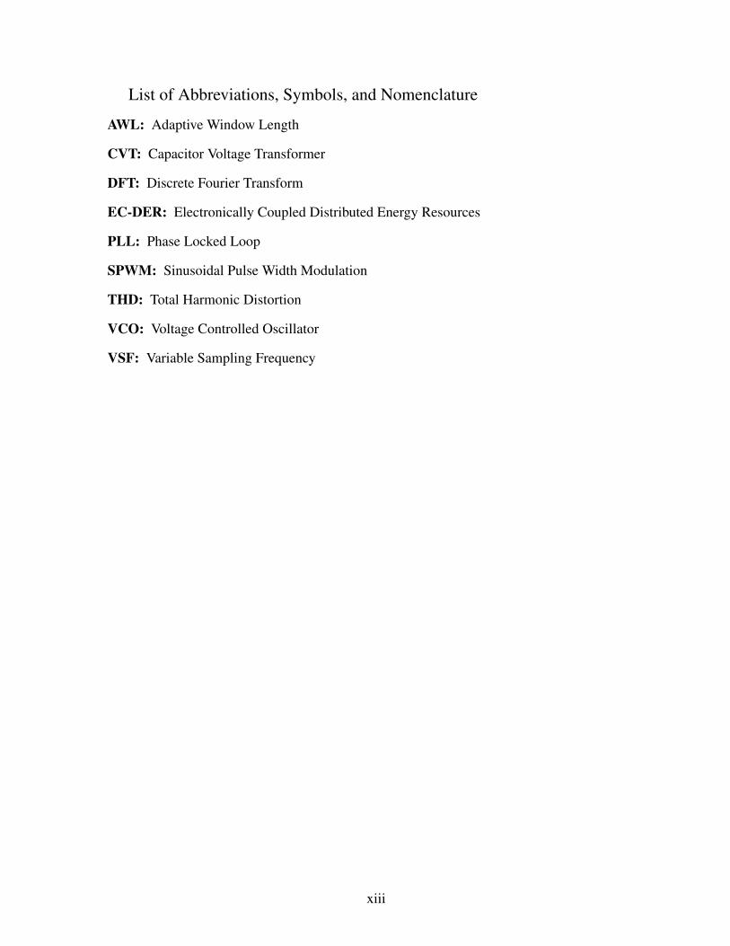
The half-bridge voltage source converter (see Figure 1.1) is the fundamental topology
which is used to introduce the voltage source converter (VSC) operation. This converter con-
sists of two bulk capacitors (C+ and C−) to split the input voltage into half and to provide
the neutral connection. The output voltage equals to Vi/2 or −Vi/2 by turning on the S + and
S −, respectively. This converter can generate a sinusoidal output voltage at the fundamental
frequency as described in [1]. If the sinusoidal pulse width modulation (SPWM) technique is
employed, low frequency harmonics will not be generated and by using appropriate filters such
as low-pass LC filters at the output of this converter, high frequency components of the voltage
waveform can be filtered out. Thus, the resultant voltage that is seen by the load becomes very
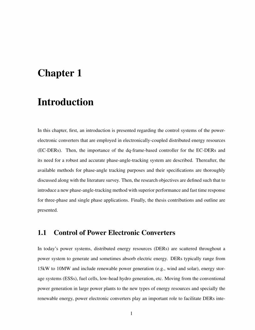
close to the fundamental component. Full-bridge converter (see Figure 1.2) is a variation of the
half-bridge converter. It will provide doubled output voltage magnitude and is recommended
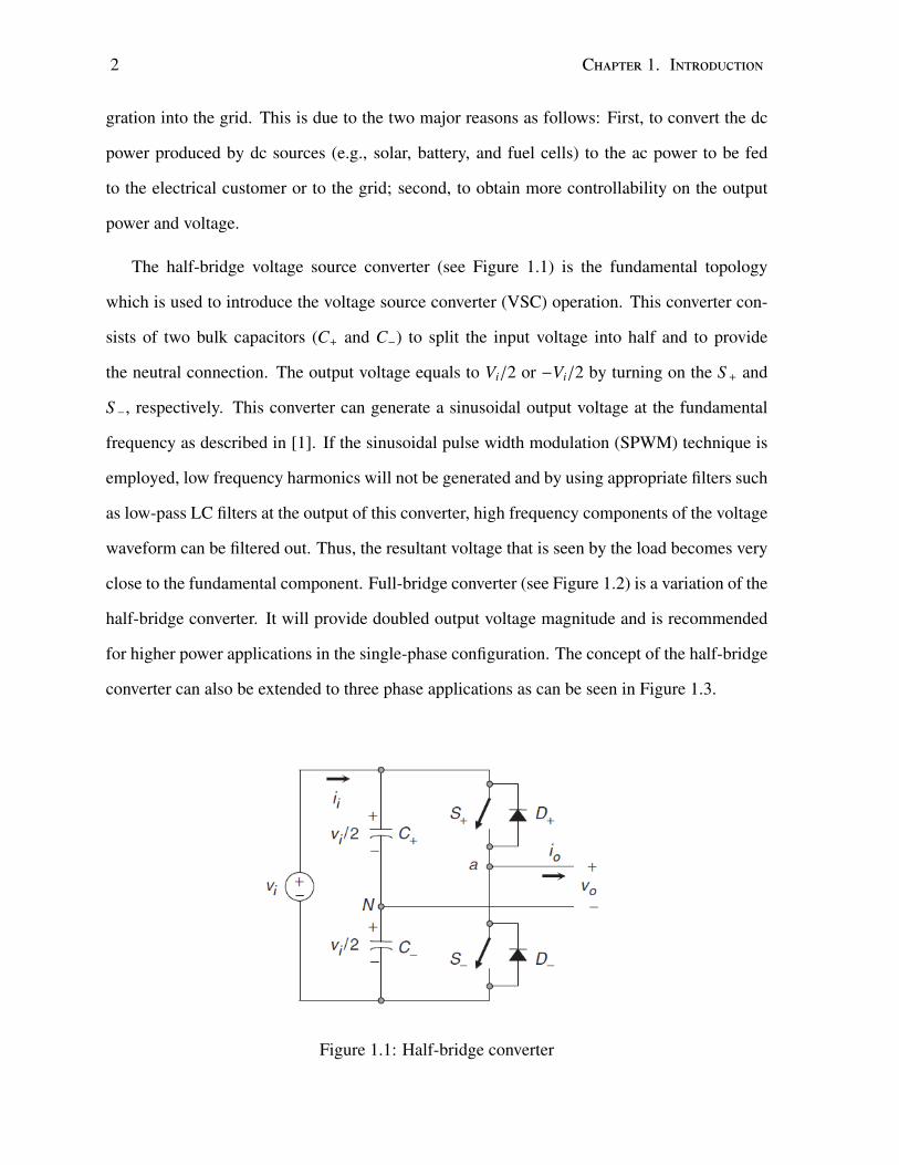
for higher power applications in the single-phase configuration. The concept of the half-bridge
converter can also be extended to three phase applications as can be seen in Figure 1.3.
Figure 1.1: Half-bridge converter
1.1. Control of Power Electronic Converters 3
Figure 1.2: Full-bridge converter
Figure 1.3: Three-phase two-level full-bridge converter
Half-bridge or full-bridge converters can be controlled by voltage- or current-mode-control
schemes. These schemes can be used depending on the application since each one has its own
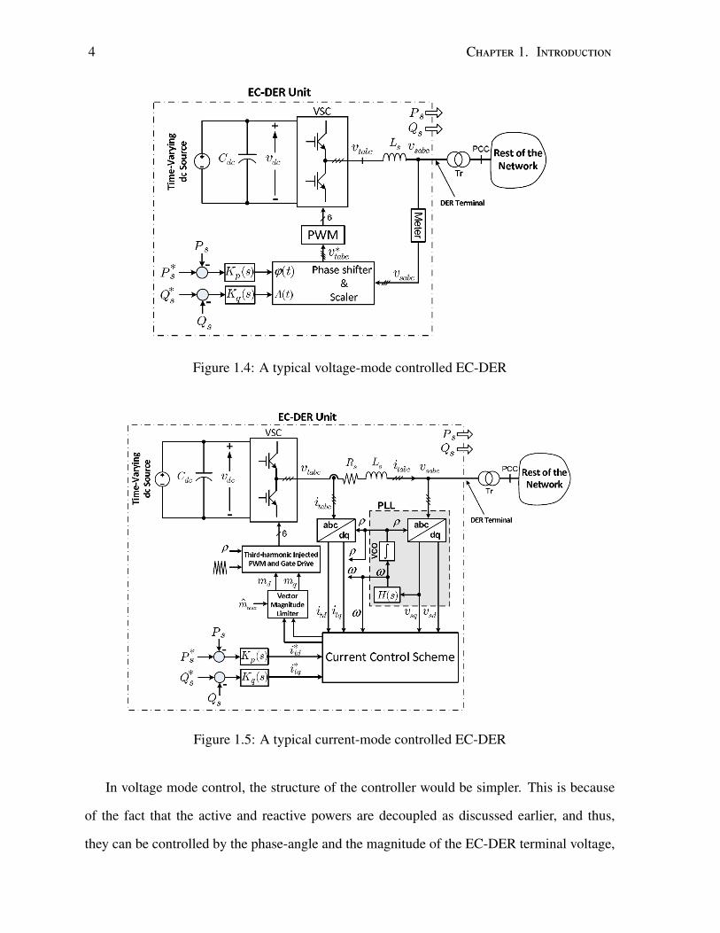
strengths and weaknesses. Figures 1.4 and 1.5 show a typical voltage-mode and current-mode
controlled electronically coupled DERs (EC-DERs), respectively.
4 Chapter 1. Introduction
Figure 1.4: A typical voltage-mode controlled EC-DER
Figure 1.5: A typical current-mode controlled EC-DER
In voltage mode control, the structure of the controller would be simpler. This is because
of the fact that the active and reactive powers are decoupled as discussed earlier, and thus,
they can be controlled by the phase-angle and the magnitude of the EC-DER terminal voltage,

1.1. Control of Power Electronic Converters 5
respectively. This can be done by two separate simple controllers. On the other hand, the
current-mode control approach can also be employed to perform the aforementioned control
functions. Although a more complex control system is needed in this case, the current mode
control approach provides some advantages over the voltage-mode control, i.e., the protec-
tion of the EC-DER against over-loading conditions and the superior dynamic performance.
Therefore, the current-mode control is a very popular approach in high power applications.
In the current-mode control technique, the converter’s AC side parameters are converted
to direct and quadrature (dq) stationary frame with an abc-to-dq transformation function as
following: fd
fq
=
cos(ρ) cos(ρ − 2π/3) cos(ρ − 4π/3)
sin(ρ) sin(ρ − 2π/3) sin(ρ − 4π/3)
fa
fb
fc
(1.1)
where fd is the direct- and fq is the quadrature-axis component. This procedure converts the
AC parameters of the grid to their equivalent dq-frame DC parameters. Consequently, the
controller design and implementation become considerably easier. This characteristic has made
the dq-frame transformation very popular in various power system applications [2].
The dq transformation is a function of the phase-angle; thus, a sinusoidal voltage phase-
angle tracking system is required to perform the dq-transformation. Traditionally, a phase-
locked loop (PLL) is employed for this purpose in the structure of the EC-DER control systems
as it is shown in Figure 1.5. The accuracy of this phase-angle tracker directly affects the
performance of the controller, thereby, that of the EC-DER. More importantly, in the presence
of other possible imperfections in the voltage signal(s) of the host network, e.g., harmonic
distortions and noise, the performance of the EC-DER will further deteriorate.

6 Chapter 1. Introduction
1.2 Phase-Angle Tracking Techniques
As discussed in the former section, accurate phase-angle tracking is required in control systems
of power-electronic converters [3]. In particular, under unbalanced and highly distorted grid
conditions, the control performance of the grid-connected voltage-sourced converters depends
on the robustness and accuracy of the estimated phase angle. This is because of the fact that
these conditions adversely affect the PLL performance whose output directly affects the con-
troller and converter performance. A faithful phase-angle-tracking method must rapidly and
accurately obtain the phase angle of the voltage/current signal(s) at the point of connection [4],
[5].
Phase-angle-tracking methods proposed for power-electronic converters can be broadly cat-
egorized into “closed-loop” and “open-loop” methods [6]. In closed-loop methods, phase-
angle of the grid voltage/current is adaptively estimated through a loop mechanism. This loop
is aimed at locking the estimated value of the phase-angle to its actual value. The concept of
PLLs has traditionally been adopted for the purpose of control and operation of power elec-
tronic converters [4], [7]-[9]. In open-loop methods, however, the estimation of the phase-angle
is directly performed through some sort of filtering techniques. The main filtering approaches
include discrete Fourier transform (DFT) [10], [11], weighted least-squares estimation [12],
Kalman filtering [10], [16], and space-vector-based methods [17].
A PLL is generally a closed-loop control system that consists of two major parts: (i) phase
detection and (ii) loop filter. In three-phase power systems, the phase detection module is nor-
mally implemented using the abc-to-dq transformation to obtain two orthogonal components
of the three-phase input signals. Figure 1.6 represents such a PLL. In this figure, the abc-dq
block (i.e., d: direct, and q: quadrature) indicates the phase-detection and the loop filter con-
sists of the compensator, saturation, and voltage-controlled oscillator (VCO) blocks. The loop
filter adjusts the rotational speed of the dq-frame (ω) so that the Vq (i.e., quadrature voltage
component) becomes zero. Then the phase-angle of the three-phase input signals (ρ) is deter-
mined by the VCO, which is a resettable integrator. The output range of this integrator is 2π

1.2. Phase-Angle Tracking Techniques 7
(e.g., −π to π).
Figure 1.6: Structure of a conventional PLL
The performance of this PLL is evaluated in Matlab Simulink through an unbalanced mag-
nitude three-phase input voltages (0.2∠0◦, 1∠ − 120◦, 1∠ − 240◦). Figure 1.7 shows the three-
phase input voltages to the PLL and the direct and quadrature voltage components after the
dq-frame transformation. As shown in this figure, a sinusoidal component with doubled grid
0.05 0.1 0.15 0.2−1
−0.5
0
0.5
1
Vab
c
0.05 0.1 0.15 0.2−0.5
0
0.5
1
1.5
Time(s)
Vdq
VaVbVc
VdVq
Figure 1.7: Performance of the conventional dq-frame-based PLL during unbalanced magni-tude three-phase input voltages

8 Chapter 1. Introduction
frequency appears after the dq-frame transformation, in both of the Vd and Vq. Thus, it gen-
erates an error in the estimated phase angle because Vq is used as the input for the loop filter.
The actual and estimated phase-angles, and the error in the estimated phase-angle are shown in
Figure 1.8.
0.05 0.1 0.15 0.20
2
4
6
8
θ (° )
0.05 0.1 0.15 0.2−20
−10
0
10
20
Time(s)
θ err (
° )
ActualEstimated
Figure 1.8: Performance of the conventional dq-frame-based PLL during unbalanced magni-tude three-phase input voltages
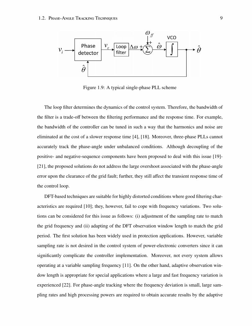
For the single-phase applications, there is only one sinusoidal signal as the input. Therefore,
the phase-detection structure is modified to generate the orthogonal component of the input
signal by different methods such as using the Park-PLL structure or creating a 90◦ delay, etc.
[13], [14], [15]. However, the time response and/or the accuracy of the PLL would be adversely
affected during this process. Figure 1.9 represents a typical scheme for the single-phase PLLs.
1.2. Phase-Angle Tracking Techniques 9
Figure 1.9: A typical single-phase PLL scheme
The loop filter determines the dynamics of the control system. Therefore, the bandwidth of
the filter is a trade-off between the filtering performance and the response time. For example,
the bandwidth of the controller can be tuned in such a way that the harmonics and noise are
eliminated at the cost of a slower response time [4], [18]. Moreover, three-phase PLLs cannot
accurately track the phase-angle under unbalanced conditions. Although decoupling of the
positive- and negative-sequence components have been proposed to deal with this issue [19]-
[21], the proposed solutions do not address the large overshoot associated with the phase-angle
error upon the clearance of the grid fault; further, they still affect the transient response time of
the control loop.
DFT-based techniques are suitable for highly distorted conditions where good filtering char-
acteristics are required [10]; they, however, fail to cope with frequency variations. Two solu-
tions can be considered for this issue as follows: (i) adjustment of the sampling rate to match
the grid frequency and (ii) adapting of the DFT observation window length to match the grid
period. The first solution has been widely used in protection applications. However, variable
sampling rate is not desired in the control system of power-electronic converters since it can
significantly complicate the controller implementation. Moreover, not every system allows
operating at a variable sampling frequency [11]. On the other hand, adaptive observation win-
dow length is appropriate for special applications where a large and fast frequency variation is
experienced [22]. For phase-angle tracking where the frequency deviation is small, large sam-
pling rates and high processing powers are required to obtain accurate results by the adaptive
10 Chapter 1. Introduction
observation window length technique.
Several phasor estimation algorithms have been proposed in literature for synchrophasor
applications to achieve higher accuracy under distorted, variable-frequency, and low-frequency
oscillatory conditions [23]. Most of these techniques utilize more than one-cycle observation
window length and require considerably more computation as compared to full-cycle DFT to
achieve higher performance. This makes them less appropriate for the phase-angle tracking in
power-electronic converters.
1.3 Research Objectives
The main objective of the proposed method is to replace the widely used closed-looped PLLs
in power-electronic converters with a new open-loop phasor-based phase-angle-tracking tech-
nique such that it provides better performance and an easier implementation. The proposed
method should be immune to harmonics, noises, voltage imbalances, and grid frequency vari-
ations; in addition, its transient response time should be limited to about one cycle (of the
nominal system frequency), and it does not require any parameter tuning as compared to PLL-
based synchronization methods [4], [7]-[8], [21]. The proposed algorithm should either work
for both single-phase and three-phase applications or two separate algorithms should be de-
vised.
1.4 Contributions
In this thesis, two different approaches are proposed for three- and single-phase applications.
The proposed single-phase method can be simply extended for the three-phase applications
while the proposed three-phase method is only applicable for three-phase applications. In the
proposed three-phase phase-angle-tracking method, the positive-sequence phase-angle needs to
be tracked for the VSC control-system applications. Therefore, a method is developed specifi-
cally for this purpose. Thus, less implementation complexity and processing power is acquired

1.4. Contributions 11
in comparison with that of when three separate single-phase PLL units are used.
In the proposed three-phase positive-sequence phase-angle-tracking algorithm, first, the er-
ror in positive-sequence phasor estimated by full-cycle-DFT is calculated analytically. Then,
the accurate positive-sequence phasor is derived based on the two proposed compensation co-
efficients. To further reduce the required processing power, an approximation is proposed to
calculate the compensation coefficients by using Taylor series expansion around the nominal
grid frequency. The aforementioned compensation coefficients are functions of the grid fre-
quency. Therefore, a robust frequency estimation method is also adopted and adjusted for the
purpose of the proposed method as part of the proposed method to accurately track the grid
frequency even during the possible abnormal grid conditions.
In Chapter 4, the single-phase configuration is proposed. In this chapter, it is analytically
presented that the error in the estimated phasor due to the off-nominal frequency operation
is more than that of the three-phase configuration. Accordingly, in addition to the phasor-
compensation, the adaptive-window length (AWL) technique is also suggested for single-phase
applications. It is noted that still fixed sampling rate is being utilized; however, by imple-
menting AWL technique, the calculated accurate phasor becomes completely immune to off-
nominal frequency operation, even beyond the standard limits. Nevertheless, AWL adversely
affects the performance of the frequency estimation method proposed for the three-phase ap-
plications. Hence, a new technique is proposed for the frequency estimation in single-phase
applications. This technique provides very accurate frequency tracking with rapid time re-
sponse. Moreover, it is immune to possible abnormal grid incidents. Later in this chapter, the
proposed method is simulated in Matlab and its performance is evaluated through extensive
study cases. Then, the hardware implementation of the proposed method is done in a digital
signal processor (DSP) and tested with an arbitrary signal generator, designed for this purpose.

12 Chapter 1. Introduction
1.5 Thesis Outline
The present thesis consists of five chapters. In the first chapter, an introduction is given to the
conducted research work. Also its contributions to the phase-angle-tracking methods used in
the EC-DER controllers are presented. In the second chapter, the phasor-estimation technique
based on the full-cycle DFT is elaborated. The impact of frequency variation on the DFT-based
phasor estimation and how to cope with them are briefly explained.
In Chapter 3, a new method is proposed for positive-sequence phase-angle tracking of the
three-phase voltage/current signals. First, the error in the estimated positive-sequence phasor
by full-cycle DFT is calculated. Then, this error is compensated using two compensation
coefficients to obtain the accurate phasor. The compensation coefficients are functions of the
grid frequency; therefore, a robust zero-crossing-based frequency-estimation method is also
adopted and adjusted for this purpose. Comprehensive simulation study is conducted using
Matlab to evaluate the performance of the proposed method for almost all of the possible grid
abnormal conditions. The comparison results with the state-of-the-art counterparts are also
included.
In Chapter 4, a phase-angle tracking method is developed for the single-phase applications,
which can be easily extended for the use in three-phase applications. To effectively reduce the
error in the estimated phasor, it is proposed to use AWL along with the phasor compensation
to gain the advantages of both and mitigate the weaknesses of both approaches. The AWL and
phasor compensation are based on the estimated grid frequency. Similar to three phase appli-
cations, a zero-crossing-based frequency-estimation technique is adopted for this purpose. It
is demonstrated that the output of the pre-filtering stage of the frequency-estimation technique
faces undesired transient as DFT window length changes due to the frequency variation. An
enhancement is proposed to effectively eliminate this issue. Extensive simulation studies are
conducted to evaluate the performance of the proposed method during the worst grid conditions
and in compliance with the standards (IEEE Std C37.118.1-2011, IEC 61000-3-6). Finally, the
simulation studies are confirmed through the hardware implementation of the proposed method

1.6. Summary 13
in a real-time DSP.
Chapter 5 summarizes the conducted research. Also, conclusions and the scope of future
works are discussed in this chapter.
1.6 Summary
In the current chapter, an introduction to the EC-DERs and their control systems was pre-
sented. Then, the importance of the phase-angle-tracking within the context of EC-DER’s
control system was discussed. A comprehensive literature survey was presented to cover all of
the state-of-the-art phase-angle-tracking methods, clarifying the advantages and disadvantages
of the different available methods and structures. Then, two research objectives including the
development of a robust and accurate phase-angle-tracking method for three-phase and single-
phase applications were presented. The research objectives were considered to improve the
accuracy and performance of the available methods and to simplify the implementation of the
algorithm. Thereafter, the research contributions were discussed, and the thesis structure was
explained.
Chapter 2
Phasor Estimation
2.1 Introduction
This chapter introduces the conventional phasor estimation technique used in power system
protection and monitoring area. First, the concept of phasor is defined. Then, the windowing
is introduced to picture the time-varient signal analysis in the power systems using phasor
estimation techniques. The DFT phasor estimation technique is discussed in detail, and the
effect of frequency variation on the estimated phasor by DFT is evaluated. Finally, possible
solutions are considered to effectively mitigate or remove the error in the estimated phasor by
DFT, caused by the frequency variation.
2.2 Phasor
The process of extraction of signal parameter (amplitude and phase angle) with respect to
power system frequency is referred to as phasor estimation [35]. Any sinusoidal signal x(t) can
be represented by its phasor form X=A∠θ. A phasor contains the information about the signal
amplitude(A) and phase angle(θ). For example, consider the following signal:
x(t) = A cos(ωt + θ) (2.1)
14
2.2. Phasor 15
Equation 2.1 can be rewritten as
x(t) = A.<(e j(ωt+θ)) (2.2)
where<(.) represents the real component of a complex number, and
X = Ae jθ = A∠θ. (2.3)
The phasor for the signal in (2.1) can be represented by (2.3) provided that the signal amplitude
(A), phase angle (θ) and angular frequency(ω) are time invariant. Use of phasor is advantages
as it converts deferential equations to algebraic equations. For example, in case of a series
RL circuit supplied by a sinusoidal source, the differential equation can be expressed in time
domain as
v(t) = Ri(t) + Ldi(t)dt
= Vm cos(ωt) (2.4)
where v(t) is the voltage signal in the time domain, R is the resistance and L is the inductance
of the circuit, i(t) is the current signal in the time domain, and the Vm is the magnitude if the
sinusoidal voltage signal. If we are only interested in steady-state response of the system, the
differential equation can be converted into an algebraic equation by applying phasor definition
to (2.4). In this case, circuit variables can be calculated simply based on other variables.
V = RI + jωLI or I =V
R + jωLor Z = R + jωL =
VI
(2.5)
where, V is the voltage phasor equals to Vm∠θv, I is the current phasor equals to Im∠θi, and Z is
the circuit impedance. Before discussing DFT-based phasor-estimation, it is very important to
understand the concept of ’windowing’ described in the next section.
2.2.1 Windowing
As discussed earlier, for defining the phasor, it has been assumed that the signal is time invari-
ant. However, in a practical power system, it is not possible to have constant signal parameters.

16 Chapter 2. Phasor Estimation
Therefore, the phasor estimation is done only for a short span of time which is often termed as
phasor estimation for a window (refer Figure 2.1).
Figure 2.1: Representation of Data Samples in a Window
This short span is generally a power system cycle which is equal to 16.67 ms for a 60 Hz
system. It is assumed that during this period, the signal parameters, i.e., magnitude (A), phase
(θ) and angular frequency (ω) are constant. The data window is continuously updated with
new samples, thereby discarding the previous samples. Thus, phasor estimation is carried out
with every new sample in order to estimate a more accurate phasor. However, the accuracy of
phasors depend upon the accuracy of samples. In the event of any disturbance or fault, these
samples undergo a transition stage which includes samples from both pre-fault and post-fault
instances as shown in Figure 2.1 by the windows with dashed lines. Therefore, in the event of
any fault, there is always a transition time equal to the size of phasor estimation window when
the estimated phasor value is not accurate.

2.3. Discrete Fourier Transform (DFT) Algorithm 17
2.3 Discrete Fourier Transform (DFT) Algorithm
In practice, power system signals, i.e., measured voltages and currents are often corrupted with
harmonics and noise. In order to accurately estimate the fundamental phasor, it is necessary
to get rid of these extra components contaminating the fundamental signal and extract only
the fundamental frequency component. Various methods have been proposed in literature for
estimating the phasors. However, discrete Fourier transform (DFT) is the most well-known
and applied technique in the area of power system protection and monitoring. The following
section describes the details of phasor estimation based on DFT.
As mentioned in the latter paragraph, DFT is the most commonly and widely used tech-
nique when it comes to protection relays environment. Extraction of a particular frequency
component is done using Fourier transform. However, in relay environment, sampled data at
discrete time steps is available for processing; therefore, the Fourier-transform calculation is
also done in discrete environment and is termed as Discrete Fourier Transform or DFT. Before
defining DFT, let us first understand Discrete-Time Fourier Transform (DTFT).
Equation (2.6) shows the mathematical representation of Fourier transform for a sampled
data signal.
X( jω) =
n=+∞∑n=−∞
x[n]e− jωn (2.6)
where, ω is 2π f / fs. Generally, a window of sampled data as discussed in the beginning of
this chapter is taken to perform Fourier analysis. Therefore, a truncated version of the above
equation is used for practical purposes. The truncated DTFT is given by (2.7).
XN( jω) =
N−1∑n=0
x[n]e− jωn (2.7)
This truncation is equivalent to multiplying by a rectangular window of data length ’N’ which
results in broadening of spectral peaks and spectral leakage, i.e., the presence of side lobes.
Let us now define a full-cyle (1-cycle) DFT where the window length is selected as N =
18 Chapter 2. Phasor Estimation
fs/ fn and the frequency of interest is fn. In power system protection, DFT is essentially the
same as DTFT, evaluated at the nominal frequency.
X =2N
N−1∑n=0
x[n]e− j2π fnfs
n (2.8)
Knowing N = fs/ fn
X =2N
N−1∑n=0
x[n]e− j2π fnN fn
n =2N
N−1∑n=0
x[n]e− j2π nN (2.9)
For a pure sinusoidal signal such as x(t) = A cos(2π fnt + θ)
x[n] = x(nfs
) = A cos(2πnN
+ θ) (2.10)
Equating x[n] into (2.9), one can get (2.11)
X =2N
N−1∑n=0
A cos(2πnN
+ θ)e− j2π nN (2.11)
Using Euler’s identity, (2.11) can be rewritten as (2.12).
X =1N
N−1∑n=0
A(e j(2π n
N +θ) + e− j(2π nN +θ)
)e− j2π n
N (2.12)
Simplifying (2.12) results into (2.13) which can further be simplified into (2.14).
X =1N
N−1∑n=0
A(e jθ + e− j(4π n
N +θ))
(2.13)
X = Ae jθ +Ae− jθ
N
N−1∑n=0
e− j4π nN (2.14)
Assuming r = e− j4π 1N of a Geometric progression (GP) series, the sum of a finite GP series is
given by (2.15).N−1∑n=0
rn = 1 + r + r2 + · · · + rN−1 =1 − rN
1 − r(2.15)

2.3. Discrete Fourier Transform (DFT) Algorithm 19
Simplifying (2.14) using (2.15), we obtain
N−1∑n=0
e− j4π nN =
1 − e− j4π NN
1 − e− j4π 1N
= 0 (2.16)
Therefore, (2.14) becomes
X( fn) = Ae jθ = A∠θ (2.17)
Equation (2.17) represents phasor for any sinusoidal signal with the fundamental frequency of
fn. Thus,
X( fn) =2N
N−1∑n=0
A cos(2πnN
+ θ)e− j2π nN (2.18)
Using (2.10) and equating into (2.18), we obtain (2.19)
X( fn) =2N
N−1∑n=0
x[n]e− j2π nN =
2N
N−1∑n=0
x[n] cos 2πnN︸ ︷︷ ︸
Xr:Real Filter
+ j2N
N−1∑n=0
−x[n] sin 2πnN︸ ︷︷ ︸
Xi:Imaginary Filter
(2.19)
Xr = Real Filter =2N
cos(2πN
n) (2.20)
Xi = Imaginary Filter = −2N
sin(2πN
n) (2.21)
where n = 0, ...,N − 1.
Phasor’s amplitude and angle can be computed by (2.22) and (2.23), respectively. In power
system protection area, it is very common to split the complex exponential term of DFT into
real and imaginary filters as shown in (2.20) and (2.21).
A =√
(Xr)2 + (Xi)2 (2.22)
∠θ = arg (Xr + jXi) (2.23)
20 Chapter 2. Phasor Estimation
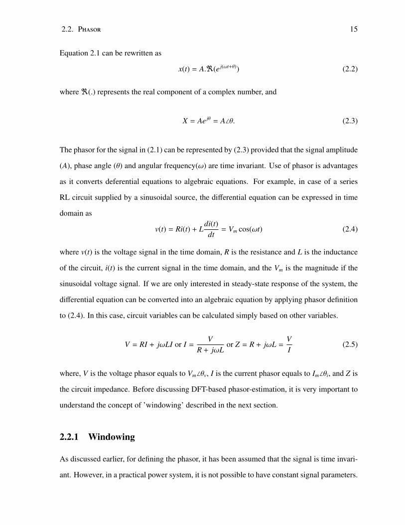
Figure 2.2: (a): Real DFT Filter (b): Imaginary DFT Filter
Figure 2.2 shows the real and imaginary filters for a 64 sample per cycle and 60 Hz power
system, represented by (2.20) and (2.21).
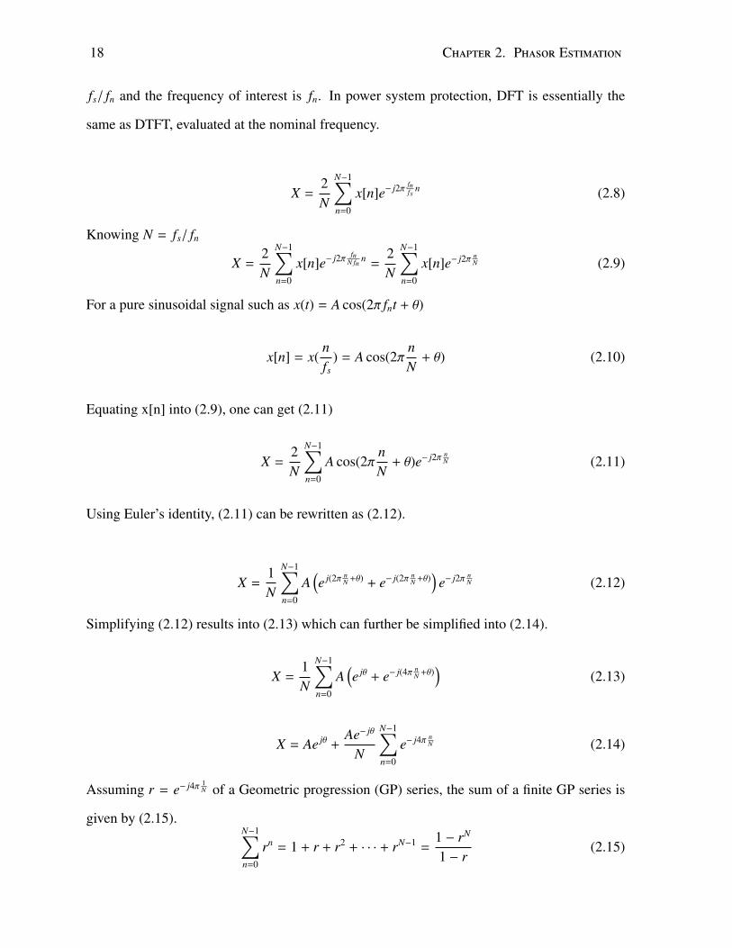
Figure 2.3: (a): Input signal (b): magnitude (c): rotating angle
2.3. Discrete Fourier Transform (DFT) Algorithm 21
x(t) = 10.cos(2π.60.t + π/6) (2.24)
Equation (2.24), represents a pure sinusoidal 60 Hz signal. Figure 2.3 (a) shows the input
signal. When the input signal is passed through DFT filters, it returns the magnitude and angle
as represented by Figure 2.3 (b) and (c). It can be observed from time response that DFT has
a transient time of 1-cycle. Also, it gives a constant phasor magnitude output for a pure 60 Hz
signal once the transient time is over. It can also be observed from the angle that it is constantly
varying. As the window of samples are updated upon acquisition of a new sample, the inherent
phase shift 2π/N occurs. Because of this phenomenon, the phasor obtained using this method
is called rotatory phasor. The estimated phasor’s phase angle is very similar to the output of
the PLL as the estimated phasor rotates in the complex plane, while the DFT sampling window
is being shifted in time.
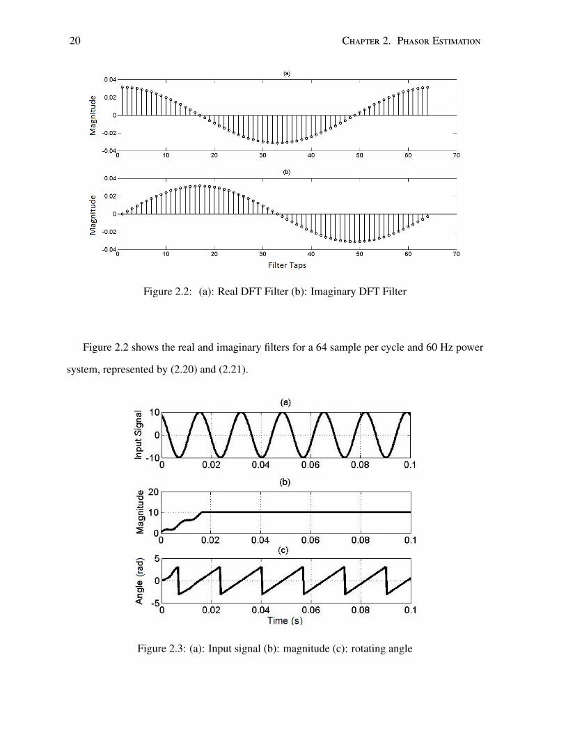
Figure 2.4: Frequency Response of 1-Cycle DFT’s Real Filter
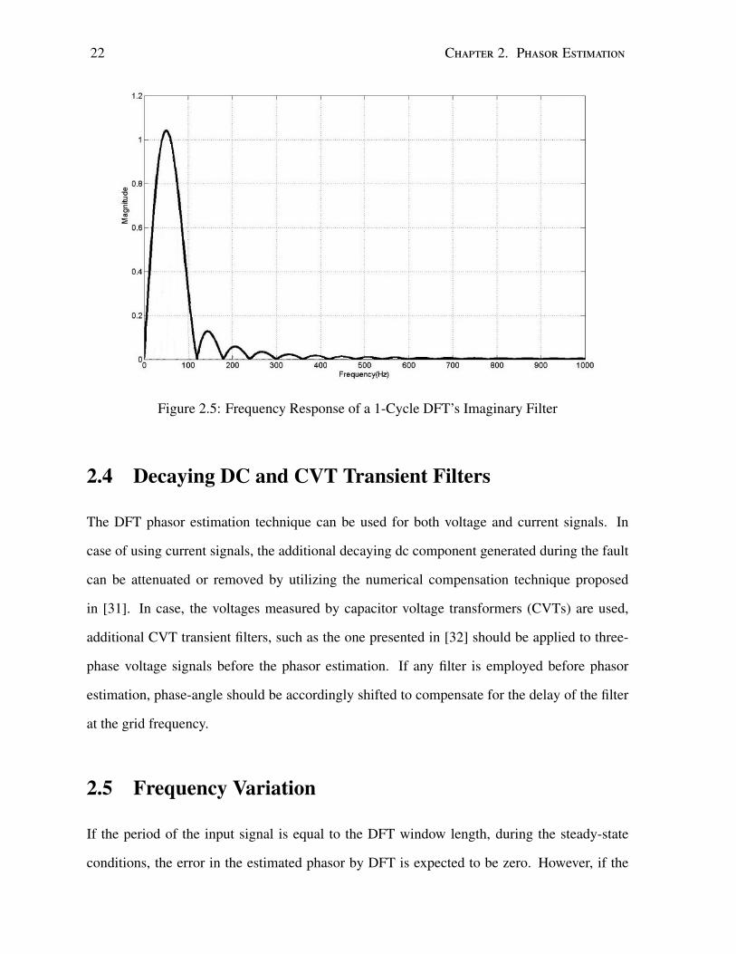
In Figure 2.4 and Figure 2.5, the frequency response of a 1-cycle DFT of real and imaginary
filters is shown. It can be observed from the real and imaginary filter’s frequency response
(magnitude) of a 1-cycle DFT that it removes DC and integer harmonics, suppresses noise, and
non-integer harmonics.
22 Chapter 2. Phasor Estimation
Figure 2.5: Frequency Response of a 1-Cycle DFT’s Imaginary Filter
2.4 Decaying DC and CVT Transient Filters
The DFT phasor estimation technique can be used for both voltage and current signals. In
case of using current signals, the additional decaying dc component generated during the fault
can be attenuated or removed by utilizing the numerical compensation technique proposed
in [31]. In case, the voltages measured by capacitor voltage transformers (CVTs) are used,
additional CVT transient filters, such as the one presented in [32] should be applied to three-
phase voltage signals before the phasor estimation. If any filter is employed before phasor
estimation, phase-angle should be accordingly shifted to compensate for the delay of the filter
at the grid frequency.
2.5 Frequency Variation
If the period of the input signal is equal to the DFT window length, during the steady-state
conditions, the error in the estimated phasor by DFT is expected to be zero. However, if the
2.5. Frequency Variation 23
grid-frequency fluctuates from its nominal value, the estimated phasor by the DFT would be
imperfect. In this case, the DFT window length can be changed so that it include more or less
samples to fit the DFT window length to the period of the input signal. Thus, the error in the es-
timated phasor by the DFT can be reduced. This is an example on how to make the DFT phasor
estimation adaptive to the grid frequency variations, and off-nominal frequency of operation.
The variable sampling frequency is another method to overcome the aforementioned problem
although its implementation is more complex than the variable window length. All of these
techniques are based on the estimated grid frequency; therefore, a robust frequency-estimation
method is inevitable for these techniques to effectively reduce the error in the estimated phasor.
DFT-based phasor-estimation is not immune to frequency variations in the input signal by
itself. However, by using techniques such as adaptive window length (AWL), variable sam-
pling frequency (VSF), and phasor compensation, the error in the estimated phasor by DFT is
prevented or compensated. AWL is a technique to change the length of the DFT filters such
that they match the period of the input signal. Thus, the AWL makes the DFT algorithm adap-
tive to the frequency variations in the input signal. The accuracy of AWL mainly depends
on the sampling resolution. Therefore, to decrease the phasor estimation error with this tech-
nique, higher sampling frequency would be required. The AWL can be useful in applications
that require wide frequency variation range and less accuracy, e.g., fast bus transfer applica-
tions. VSF, however, keeps the number of samples in the DFT filters constant, and adjusts
the sampling frequency to match the DFT window length with the period of the fundamental
frequency component. The VSF is useful where a narrow range of changes of frequency but a
higher accuracy is expected. As such, VSF is the most popular technique used in the protection
relays.
Another approach to make the DFT adaptive to the frequency variation is phasor compen-
sation. This can be done by calculating the error caused by the off-nominal frequency operation
in the DFT phasor-estimation and then, to compensate the imperfect phasor to obtain the accu-
rate phasor. Frequency estimation is required in this technique to calculate the compensation
24 Chapter 2. Phasor Estimation
coefficients. The advantage of this method is the simplicity of implementation because it does
not require any hardware modifications and it adds negligible calculation burden to the con-
ventional DFT. Nevertheless, by compensating the error that is caused by the fundamental
frequency component while the signal is contaminated with harmonics during the off-nominal
frequency operation, the errors caused by harmonics appear in the estimated phasor. This is
due to the fact that full cycle DFT filters tuned to the nominal frequency do not fully eliminate
harmonics during off-nominal frequency operation. This error increases by deviating from the
fundamental frequency. Therefore, phasor compensation is not recommended if higher accu-
racy is needed during considerable off-nominal frequency operation with distorted signals.
2.5.1 Off-Nominal Frequency Operation with Conventional DFT
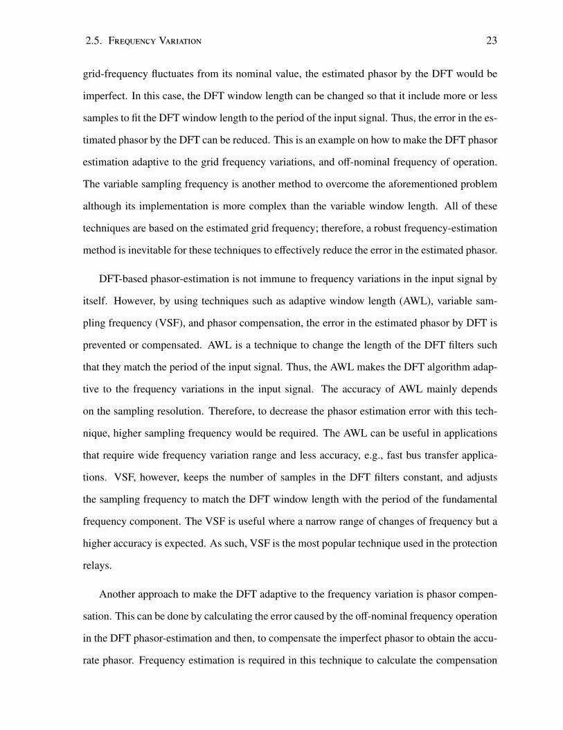
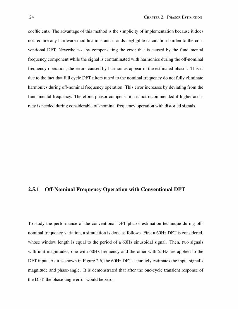
To study the performance of the conventional DFT phasor estimation technique during off-
nominal frequency variation, a simulation is done as follows. First a 60Hz DFT is considered,
whose window length is equal to the period of a 60Hz sinusoidal signal. Then, two signals
with unit magnitudes, one with 60Hz frequency and the other with 55Hz are applied to the
DFT input. As it is shown in Figure 2.6, the 60Hz DFT accurately estimates the input signal’s
magnitude and phase-angle. It is demonstrated that after the one-cycle transient response of
the DFT, the phase-angle error would be zero.
2.5. Frequency Variation 25
Figure 2.6: DFT response during nominal frequency operation
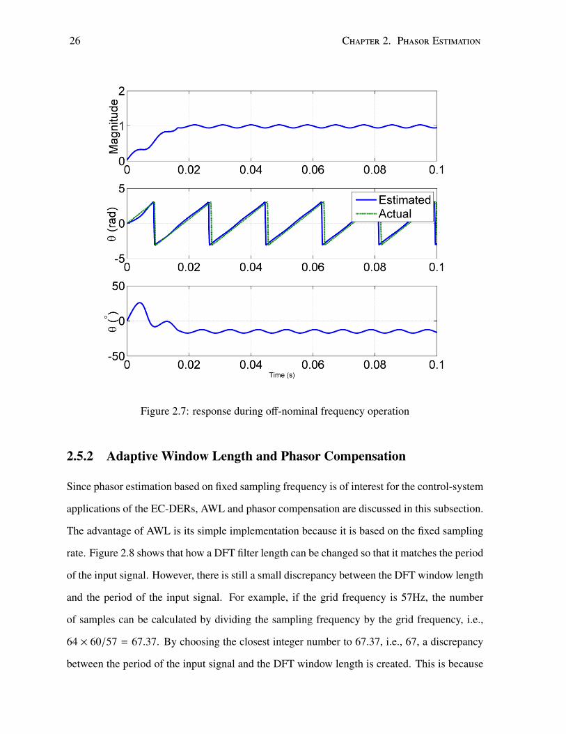
For the 55Hz signal, however, the estimated phasor by the 60Hz DFT will be imperfect both
in magnitude and phase-angle. This is shown in Figure 2.7. Although the error in magnitude
is not very high, the error in the phase-angle is considerable. Therefore, in order to use the
conventional DFT as a phase-angle tracking method, this error needs to be effectively reduced
or compensated.
26 Chapter 2. Phasor Estimation
Figure 2.7: response during off-nominal frequency operation
2.5.2 Adaptive Window Length and Phasor Compensation
Since phasor estimation based on fixed sampling frequency is of interest for the control-system
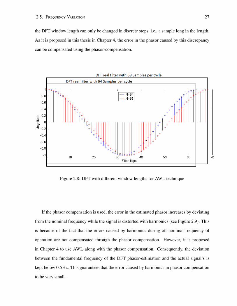
applications of the EC-DERs, AWL and phasor compensation are discussed in this subsection.
The advantage of AWL is its simple implementation because it is based on the fixed sampling
rate. Figure 2.8 shows that how a DFT filter length can be changed so that it matches the period
of the input signal. However, there is still a small discrepancy between the DFT window length
and the period of the input signal. For example, if the grid frequency is 57Hz, the number
of samples can be calculated by dividing the sampling frequency by the grid frequency, i.e.,
64 × 60/57 = 67.37. By choosing the closest integer number to 67.37, i.e., 67, a discrepancy
between the period of the input signal and the DFT window length is created. This is because
2.5. Frequency Variation 27
the DFT window length can only be changed in discrete steps, i.e., a sample long in the length.
As it is proposed in this thesis in Chapter 4, the error in the phasor caused by this discrepancy
can be compensated using the phasor-compensation.
Figure 2.8: DFT with different window lengths for AWL technique
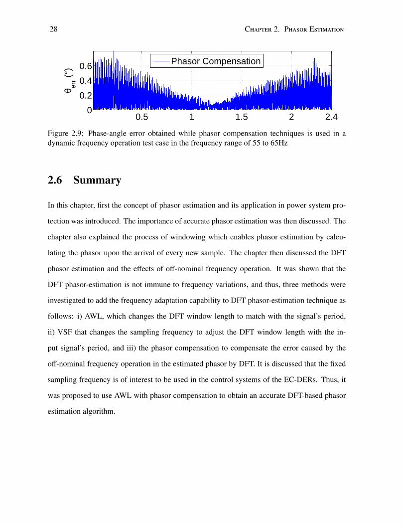
If the phasor compensation is used, the error in the estimated phasor increases by deviating
from the nominal frequency while the signal is distorted with harmonics (see Figure 2.9). This
is because of the fact that the errors caused by harmonics during off-nominal frequency of
operation are not compensated through the phasor compensation. However, it is proposed
in Chapter 4 to use AWL along with the phasor compensation. Consequently, the deviation
between the fundamental frequency of the DFT phasor-estimation and the actual signal’s is
kept below 0.5Hz. This guarantees that the error caused by harmonics in phasor compensation
to be very small.
28 Chapter 2. Phasor Estimation
0.5 1 1.5 2 2.40
0.2
0.4
0.6θ er
r (°)
Phasor Compensation
(b)
Figure 2.9: Phase-angle error obtained while phasor compensation techniques is used in adynamic frequency operation test case in the frequency range of 55 to 65Hz
2.6 Summary
In this chapter, first the concept of phasor estimation and its application in power system pro-
tection was introduced. The importance of accurate phasor estimation was then discussed. The
chapter also explained the process of windowing which enables phasor estimation by calcu-
lating the phasor upon the arrival of every new sample. The chapter then discussed the DFT
phasor estimation and the effects of off-nominal frequency operation. It was shown that the
DFT phasor-estimation is not immune to frequency variations, and thus, three methods were
investigated to add the frequency adaptation capability to DFT phasor-estimation technique as
follows: i) AWL, which changes the DFT window length to match with the signal’s period,
ii) VSF that changes the sampling frequency to adjust the DFT window length with the in-
put signal’s period, and iii) the phasor compensation to compensate the error caused by the
off-nominal frequency operation in the estimated phasor by DFT. It is discussed that the fixed
sampling frequency is of interest to be used in the control systems of the EC-DERs. Thus, it
was proposed to use AWL with phasor compensation to obtain an accurate DFT-based phasor
estimation algorithm.

Chapter 3
Positive-Sequence Phase-Angle Tracking
3.1 Introduction
In this chapter, a positive-sequence phase-angle tracking method is proposed for three-phase
applications. Although the proposed method is elaborated for voltage signals, it can also be
applied to current signals, e.g., for series-connected converters. In Section 3.2, the DFT error
associated with the calculation of the positive-sequence phasor in a variable-frequency envi-
ronment is accurately formulated. Then, the accurate phase-angle is calculated based on the
estimated positive- and negative-sequence of the voltage phasors, estimated frequency, and
two proposed compensation coefficients. Moreover, a simple approximation is proposed to
reduce the processing power required to compute two compensation coefficients. In Section
3.3, five comprehensive case studies are conducted in the Matlab software environment to eval-
uate the performance of the proposed method. Although it is not common to test the phase-
angle-estimation methods towards interharmonics, comprehensive interharmonic tests are also
conducted in this chapter. Finally, the conclusions and comparison with the state-of-the-art
methods are presented in Section 3.5.
29

30 Chapter 3. Positive-Sequence Phase-Angle Tracking
3.2 Proposed Phasor Measurement Algorithm
3.2.1 Phase-Angle Measurement of Positive-Sequence Components using
Standard DFT
To determine the DFT error for positive-sequence phasor estimation under off-nominal fre-
quency operation, let us consider the phasor of a voltage signal estimated by a full-cycle DFT.
Equation (3.1) represents a given voltage signal in a discrete-time domain.
v[n] = Vm cos(2π fg
N fnn + θ0
)(3.1)
where v[n] is the discrete form of a continuous-time signal sampled at the rate of N samples per
fundamental-component cycle, and n specifies the sample number. Vm is the signal magnitude,
and θ0 denotes the angle at n = 0. The grid actual and nominal frequencies are fg and fn,
respectively. According to the definition of full-cycle DFT, the fundamental-frequency phasor
(V) of a discrete voltage signal v[n] can be represented as
V =2N
N−1∑n=0
v[n]e− j 2πN n. (3.2)
If the grid frequency fg equals the nominal frequency fn, the voltage phasor of v[n] is calculated
as V = Vme jθ0 = Vm∠θ0. However, if the grid frequency deviates from its nominal value,
the phasor estimation using standard DFT is inaccurate. Assuming that the grid frequency is
known but different from the nominal frequency, the fundamental-frequency phasor of v[n] can
be written as
Ves =2N
N−1∑n=0
Vm cos (2πN
fg
fnn + θ0)e− j 2π
N n (3.3)
where Ves is the estimated voltage-phasor using full-cycle DFT. In a full-cycle DFT algorithm,
acquisition of a new sample is equivalent to forward shifting of the signal samples in time
domain. Therefore, the estimated phase-angle inherently increases by 2π/N once a new sample
3.2. Proposed PhasorMeasurement Algorithm 31
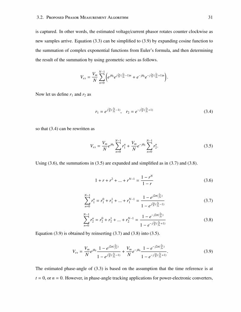
is captured. In other words, the estimated voltage/current phasor rotates counter clockwise as
new samples arrive. Equation (3.3) can be simplified to (3.9) by expanding cosine function to
the summation of complex exponential functions from Euler’s formula, and then determining
the result of the summation by using geometric series as follows.
Ves =Vm
N
N−1∑n=0
(e jθ0e j 2π
N (fgfn−1)n + e− jθ0e− j 2π
N (fgfn
+1)n).
Now let us define r1 and r2 as
r1 = e j 2πN (
fgfn−1), r2 = e− j 2π
N (fgfn
+1) (3.4)
so that (3.4) can be rewritten as
Ves =Vm
Ne jθ0
N−1∑n=0
rn1 +
Vm
Ne− jθ0
N−1∑n=0
rn2. (3.5)
Using (3.6), the summations in (3.5) are expanded and simplified as in (3.7) and (3.8).
1 + r + r2 + ... + rN−1 =1 − rN
1 − r(3.6)
N−1∑n=0
rn1 = r0
1 + r11 + ... + rN−1
1 =1 − e j2π(
fgf n )
1 − e j 2πN (
fgfn−1)
(3.7)
N−1∑n=0
rn2 = r0
2 + r12 + ... + rN−1
2 =1 − e− j2π(
fgfn
)
1 − e− j 2πN (
fgfn
+1)(3.8)
Equation (3.9) is obtained by reinserting (3.7) and (3.8) into (3.5).
Ves =Vm
Ne jθ0
1 − e j2π(fgf n )
1 − e j 2πN (
fgfn−1)
+Vm
Ne− jθ0
1 − e− j2π(fgfn
)
1 − e− j 2πN (
fgfn
+1). (3.9)
The estimated phase-angle of (3.3) is based on the assumption that the time reference is at
t = 0, or n = 0. However, in phase-angle tracking applications for power-electronic converters,
32 Chapter 3. Positive-Sequence Phase-Angle Tracking
the real-time phase-angle of the voltage waveform is needed to be measured. Thus, we would
like to determine the phase-angle of the measured signal at the last acquired sample, i.e., at the
present time. According to (3.1), the phase-angle at the last acquired sample, i.e., n = N − 1
can be specified as
θN−1 = 2πfg
fn
(1 −
1N
)+ θ0 (3.10)
where θN−1 is the phase-angle of the voltage signal considering the time of the last sample
acquisition as the reference time. Similarly, the phasor of the voltage signal considering the
last sample acquisition as the reference time can be calculated. This phasor is referred to as the
accurate phasor VAcc, and given by
VAcc = Vme j(2π
fgfn (1− 1
N )+θ0
). (3.11)
Since it is required to track the angle of the accurate phasor for phase-angle-tracking applica-
tions, the estimated phasor in (3.9) needs to be written in terms of VAcc. In reference to the
terms in (3.9), for the sake of simplification it is better to write this equation in terms of VAcc
and V∗Acc, where ’∗’ denotes the complex conjugate. Therefore, the first and second terms in
the right hand side of (3.9) are multiplied with and divided by exp( j(2π fg/ fn(1 − 1/N))) and
exp(− j(2π fg/ fn(1 − 1/N))), respectively as below.
Ves =Vm
Ne jθ0
e j(2π
fgfn (1− 1
N ))
e j(2π
fgfn (1− 1
N )) 1 − e j2π
fgf n
1 − e j 2πN
(fgfn−1
) +Vm
Ne− jθ0
e− j(2π
fgfn (1− 1
N ))
e− j(2π
fgfn (1− 1
N )) 1 − e− j2π
fgfn
1 − e− j 2πN
(fgfn
+1) (3.12)
By extracting VAcc and V∗Acc as per (3.11), (3.12) can be written as
Ves = VAcc1N
e− j(2π
fgfn (1− 1
N )) (
1 − e j2πfgfn
)1 − e j 2π
N
(fgfn−1
) + V∗Acc1N
e j(2π
fgfn (1− 1
N )) (
1 − e− j2πfgfn
)1 − e− j 2π
N
(fgfn
+1)
3.2. Proposed PhasorMeasurement Algorithm 33
= VAcc1N
(e− j2π
fgfn − 1
)(e− j2π
fgN fn − e− j 2π
N
) + V∗Acc1N
(e j2π
fgfn − 1
)(e j2π
fgN fn − e− j 2π
N
)
= VAcc1N
e− jπfgfn
(e− jπ
fgfn − e jπ
fgfn
)e− j 2π
N e j πN
(1−
fgfn
) (e j πN
(1−
fgfn
)− e− j πN
(1−
fgfn
)) + V∗Acc1N
e jπfgfn
(e jπ
fgfn − e− jπ
fgfn
)e− j 2π
N e j πN
(1+
fgfn
) (e j πN
(1+
fgfn
)− e− j πN
(1+
fgfn
))
= VAcc
sin(π
fgfn
)N sin
(πN
( fgfn− 1
))e jπ(
fgfn ( 1−N
N )+ 1N
)
︸ ︷︷ ︸k1
+V∗Acc
sin(π
fgfn
)N sin
(πN
( fgfn
+ 1))e jπ
(fgfn ( N−1
N )+ 1N
)
︸ ︷︷ ︸k2
. (3.13)
Thus, the estimated phasor can be written in terms of VAcc and its complex conjugate V∗Acc as in
Ves = k1VAcc + k2V∗Acc. (3.14)
In (3.14), k1 and k2 are defined as follows:
k1 = k1Mag∠k1Ang, k2 = k2Mag∠k2Ang (3.15)
in which,
k1Mag =1N
sin(π( fg
fn− 1
))sin
(πN
( fgfn− 1
)) , k1Ang = π
(1 − N
N
) (fg
fn+ 1
)(3.16)
k2Mag =1N
sin(π( fg
fn+ 1
))sin
(πN
( fgfn
+ 1)) , k2Ang = π
(N − 1
N
) (fg
fn− 1
). (3.17)
Equation (3.14) shows that the estimated phasor has a linear relationship with the accurate
phasor and its complex conjugate for a given grid frequency. In this equation, k1 and k2 are the
compensation coefficients. It is noted that the compensation coefficients are neither sensitive
to the signal magnitude nor to the angle. Further, they are time invariant and are only functions
of the grid frequency. Magnitude and angle of k1 and k2 for a frequency range of 55Hz to 65
Hz are shown in Figure 3.1. As it is shown, the magnitude of k1 is very close to one and only
34 Chapter 3. Positive-Sequence Phase-Angle Tracking
deviates 1.14% by a 5-Hz frequency deviation. Further, the relationship of k1 magnitude with
frequency is very similar to a quadratic function. Figure 3.1 also illustrates that the magnitude
of k2 is very close to zero and deviates 4.3% by a 5-Hz frequency deviation. Besides, the
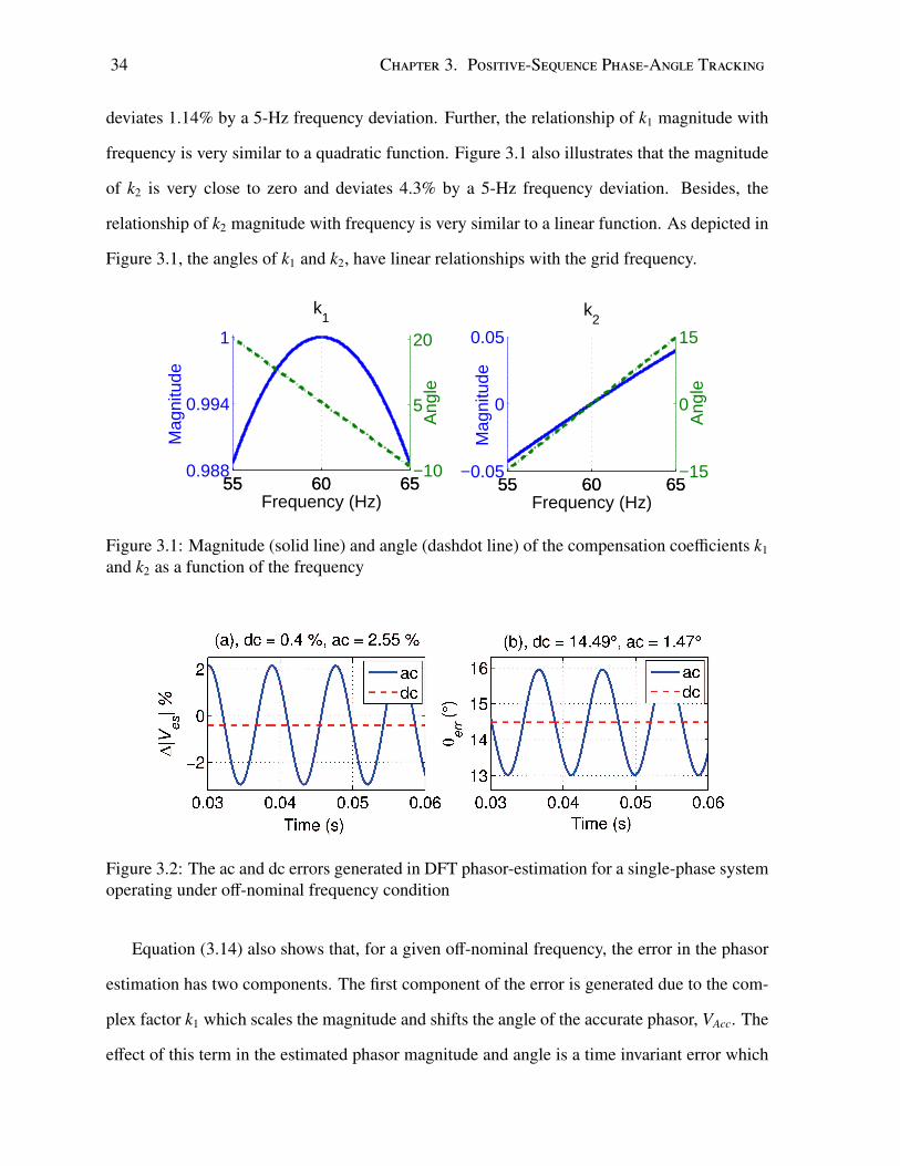
relationship of k2 magnitude with frequency is very similar to a linear function. As depicted in
Figure 3.1, the angles of k1 and k2, have linear relationships with the grid frequency.
55 60 650.988
0.994
1
Frequency (Hz)
Mag
nitu
de
k1
55 60 65−10
5
20
Ang
le
55 60 65−0.05
0
0.05
Frequency (Hz)M
agni
tude
k2
55 60 65−15
0
15
Ang
le
Figure 3.1: Magnitude (solid line) and angle (dashdot line) of the compensation coefficients k1
and k2 as a function of the frequency
Figure 3.2: The ac and dc errors generated in DFT phasor-estimation for a single-phase systemoperating under off-nominal frequency condition
Equation (3.14) also shows that, for a given off-nominal frequency, the error in the phasor
estimation has two components. The first component of the error is generated due to the com-
plex factor k1 which scales the magnitude and shifts the angle of the accurate phasor, VAcc. The
effect of this term in the estimated phasor magnitude and angle is a time invariant error which

3.2. Proposed PhasorMeasurement Algorithm 35
is, hereinafter, referred to as the “dc error”. The second component of the error, however, is
generated through the scaling of the magnitude and shifting the angle of the accurate phasor
conjugate, V∗Acc. Since V∗Acc rotates clockwise, the error generated by this component has a
sinusoidal shape whose frequency is twice of the grid frequency; thus, it is called “ac error”
in this thesis. This fact is illustrated in Figs. 3.2.(a) and (b), where the magnitude (∆|Ves|)
and phase-angle errors (θerr) of a 57-Hz sinusoidal signal are indicated, respectively. As it is
shown, the errors have both dc and ac components. For a 57-Hz sinusoidal signal, the error in
magnitude is only 0.4% dc and 2.55% peak ac; however, the error in phasor angle is 14.49◦
dc and 1.47◦ peak ac, which are considerable. Equation (3.14) can separately be reiterated for
each phase of a three-phase system as
VaDFT = k1VaAcc + k2V∗aAcc (3.18)
VbDFT = k1VbAcc + k2V∗bAcc (3.19)
VcDFT = k1VcAcc + k2V∗cAcc (3.20)
where VaAcc, VbAcc, and VcAcc are the three-phase accurate voltage phasors, and VaDFT , VbDFT ,
and VcDFT are the estimated phasors of three-phase voltages obtained by full-cycle DFT. Ap-
plying the Fortescue’s transform, the positive-sequence voltage phasor is obtained as
VposDFT = 13 (VaDFT + αVbDFT + α2VcDFT )
= 13k1(VaAcc + αVbAcc + α2VcAcc)
+ 13k2(VaAcc + α2VbAcc + αVcAcc)∗
= k1VposAcc + k2V∗negAcc (3.21)
where α = 1∠120◦, VposDFT is the positive sequence of the estimated voltage phasors, VposAcc is
the positive sequence of accurate voltage phasors, and V∗negAcc is the complex conjugate of the
negative sequence of accurate voltage phasors. Similar to the equation derived for single-phase

36 Chapter 3. Positive-Sequence Phase-Angle Tracking
phasor estimation, the error of the estimated positive-sequence phasor has two components.
The first component generates dc error, while the second component generates ac error. Figure
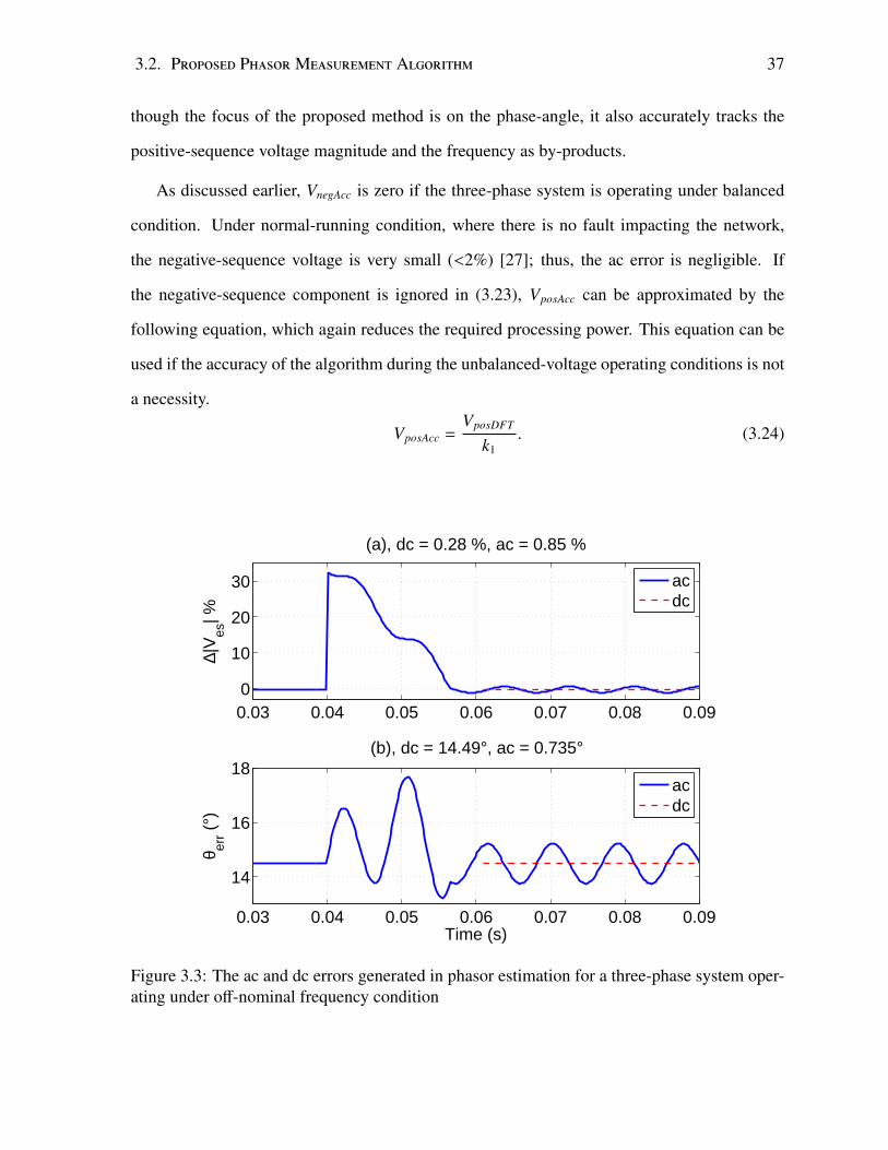
3.3 shows the error in magnitude and angle of the estimated positive-sequence phasor for a
57-Hz three-phase sinusoidal signal. The three-phase voltages are balanced until t = 0.04
s and, then, phase-C voltage is forced to zero to simulate a severe single-phase-to-ground
fault. As it is shown in the figure, the ac component of errors in both magnitude and phase-
angle is zero before the fault occurrence. This is due to the fact that the three-phase voltage
is balanced and, thus, there is no negative-sequence component. Once the fault takes place,
the negative-sequence component significantly increases; hence, the ac error of the estimated
positive-sequence phasor is expected to grow. As illustrated in Figure 3.3, once DFT transient
disappears, i.e., at t = 0.04 + 0.0167 = 0.0567s, the error in magnitude is 0.28% dc and
0.85% ac peak, while the angle error is 14.49◦ dc and 0.735◦ ac peak. It is evident that the dc
component of the phase-angle error is significant, while its ac component is quite negligible,
even during a solid close-in single-phase-to-ground fault. Similar approach to the one adopted
in (3.21) can be employed to determine the negative-sequence component of the estimated
voltage phasors as
VnegDFT = k1VnegAcc + k2V∗posAcc (3.22)
where VnegDFT is the negative sequence of the estimated phasors, VnegAcc is the negative se-
quence of the accurate voltage phasors, and V∗posAcc is the complex conjugate of the positive
sequence of the accurate voltage phasors. Assuming k1 and k2 are known and solving for
(3.21) and (3.22), VposAcc can be calculated as
VposAcc =k∗1VposDFT − k2V∗negDFT
|k1|2− |k2|
2 . (3.23)
The recent equation is the base of the proposed algorithm for accurate phase-angle tracking
purposes, which is implemented in the Error Compensation Unit block in Figure 3.4. Even
3.2. Proposed PhasorMeasurement Algorithm 37
though the focus of the proposed method is on the phase-angle, it also accurately tracks the
positive-sequence voltage magnitude and the frequency as by-products.
As discussed earlier, VnegAcc is zero if the three-phase system is operating under balanced
condition. Under normal-running condition, where there is no fault impacting the network,
the negative-sequence voltage is very small (<2%) [27]; thus, the ac error is negligible. If
the negative-sequence component is ignored in (3.23), VposAcc can be approximated by the
following equation, which again reduces the required processing power. This equation can be
used if the accuracy of the algorithm during the unbalanced-voltage operating conditions is not
a necessity.
VposAcc =VposDFT
k1. (3.24)
0.03 0.04 0.05 0.06 0.07 0.08 0.090
10
20
30
∆|V
es| %
(a), dc = 0.28 %, ac = 0.85 %
acdc
0.03 0.04 0.05 0.06 0.07 0.08 0.09
14
16
18
Time (s)
θ err (
°)
(b), dc = 14.49°, ac = 0.735°
acdc
Figure 3.3: The ac and dc errors generated in phasor estimation for a three-phase system oper-ating under off-nominal frequency condition
38 Chapter 3. Positive-Sequence Phase-Angle Tracking
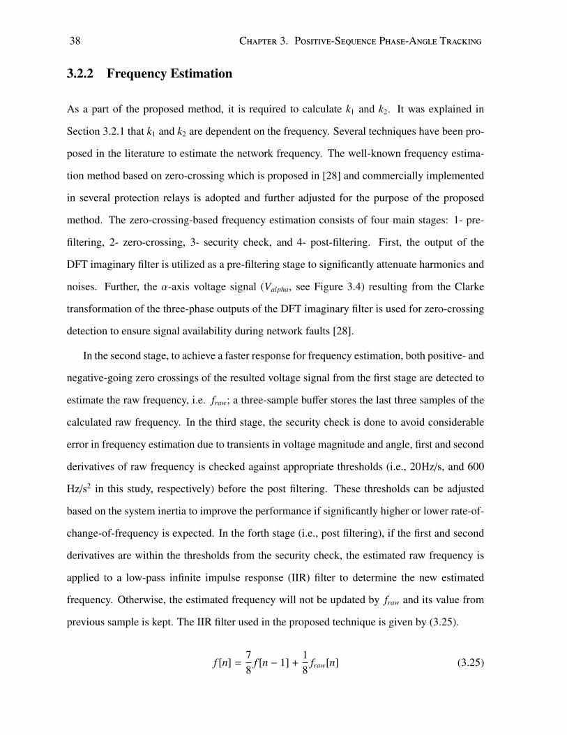
3.2.2 Frequency Estimation
As a part of the proposed method, it is required to calculate k1 and k2. It was explained in
Section 3.2.1 that k1 and k2 are dependent on the frequency. Several techniques have been pro-
posed in the literature to estimate the network frequency. The well-known frequency estima-
tion method based on zero-crossing which is proposed in [28] and commercially implemented
in several protection relays is adopted and further adjusted for the purpose of the proposed
method. The zero-crossing-based frequency estimation consists of four main stages: 1- pre-
filtering, 2- zero-crossing, 3- security check, and 4- post-filtering. First, the output of the
DFT imaginary filter is utilized as a pre-filtering stage to significantly attenuate harmonics and
noises. Further, the α-axis voltage signal (Valpha, see Figure 3.4) resulting from the Clarke
transformation of the three-phase outputs of the DFT imaginary filter is used for zero-crossing
detection to ensure signal availability during network faults [28].
In the second stage, to achieve a faster response for frequency estimation, both positive- and
negative-going zero crossings of the resulted voltage signal from the first stage are detected to
estimate the raw frequency, i.e. fraw; a three-sample buffer stores the last three samples of the
calculated raw frequency. In the third stage, the security check is done to avoid considerable
error in frequency estimation due to transients in voltage magnitude and angle, first and second
derivatives of raw frequency is checked against appropriate thresholds (i.e., 20Hz/s, and 600
Hz/s2 in this study, respectively) before the post filtering. These thresholds can be adjusted
based on the system inertia to improve the performance if significantly higher or lower rate-of-
change-of-frequency is expected. In the forth stage (i.e., post filtering), if the first and second
derivatives are within the thresholds from the security check, the estimated raw frequency is
applied to a low-pass infinite impulse response (IIR) filter to determine the new estimated
frequency. Otherwise, the estimated frequency will not be updated by fraw and its value from
previous sample is kept. The IIR filter used in the proposed technique is given by (3.25).
f [n] =78
f [n − 1] +18
fraw[n] (3.25)

3.2. Proposed PhasorMeasurement Algorithm 39
where f [n] denotes the estimated frequency after post-filtering, and fraw[n] is the calculated
raw frequency at the real time.
3.2.3 Approximation of the Compensating Coefficients
It was discussed in Section 3.2.1 that the two compensation coefficients (i.e., k1 and k2) are
complex functions of the grid frequency. If the direct computation of k1 and k2 in real-time
exceeds the available processing capacity, an accurate approximation technique can be em-
ployed to significantly reduce the computation requirements. This section proposes such an
approximation procedure.
As explained in Section 3.2.1, k1Ang and k2Ang are linear functions of the grid frequency
while k1Mag and k2Mag are trigonometric functions of fg. Thus, k1Mag and k2Mag can be approx-
imated by their Taylor series expanded around the nominal frequency ( fn). Since k1Mag and
k2Mag resemble quadratic and linear functions, respectively, second order and first order Taylor
series approximations are employed as shown in (3.26) and (3.27), respectively. It should be
noted that the discrepancy between the approximated and accurate values within the range of
interest, i.e. 55Hz to 65Hz, is less than 3.9 × 10⁻⁵ and 1.9 × 10⁻³ for k1 and k2, respectively.
k1Mag = 1 −C1( fg − fn)2 (3.26)
k2Mag = C2( fg − fn) (3.27)
where C1 = 0.00045681, and C2 = 0.0083 are calculated for N = 64 and fn = 60Hz.

40 Chapter 3. Positive-Sequence Phase-Angle Tracking
3.3 Simulation Study and Results
3.3.1 Simulation Settings
A Matlab model is developed to evaluate the performance of the proposed method for different
operational conditions including harmonic interference, noise distortion, voltage dip, phase-
angle jump, off-nominal frequency, and dynamic frequency deviation. Figure 3.4 illustrates
the block diagram of the proposed method implemented in Matlab. The test signals are first
generated at 10 times of the sampling rate which is fs = 64 × 60 = 3840Hz in this chapter.
As investigated in this study, a sampling rate greater than 64 samples per cycle does not con-
siderably reduce the sidelobes’ magnitude of the DFT frequency response and, thereby, the
algorithm performance. Then, the generated signals are passed through a typical anti-aliasing
filter used in power system protection and control applications. After the anti-aliasing filter,
the filtered signals are decimated ten times to reach the design sampling rate. This method
of signal generation is adopted to properly simulate analog anti-aliasing filter with its digital
equivalent. It further allows the modeling of high-order harmonics and high-frequency noises.
A fourth-order Butterworth low-pass digital filter with cut-off frequency of 1536Hz (=0.4 fs) is
selected to prevent aliasing (see Anti-Aliasing Filter block in Figure 3.4). The delay caused by
the anti-aliasing filter is compensated adaptively based on the estimated frequency. A full-cycle
DFT algorithm is employed to estimate the phasor of three-phase voltages. Positive and nega-
tive sequences of three-phase voltages are calculated (see Sequence Calculator block in Figure
3.4) as discussed in Section 3.2.1. The grid frequency fg is estimated using the zero-crossing
technique as described in Section 3.2.2. Having VposDFT , VnegDFT , and fg, the error compen-
sation unit calculates approximated values of k1 and k2 (as described in Section 3.2.3), and
thereby VposAcc. The entire process of angle estimation is executed at the sampling frequency,
i.e., 3840Hz.
The major computational burden of the proposed method is as follows: i) DFT for three
phases requires 384 multiplications and 192 summation at each data sample acquisition; ii)
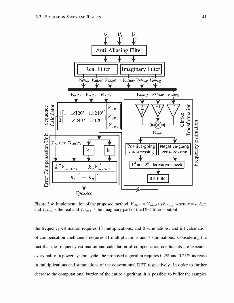
3.3. Simulation Study and Results 41
Figure 3.4: Implementation of the proposed method; VxDFT = VxReal+ jVxImag, where x = a, b, c,and VxReal is the real and VxImag is the imaginary part of the DFT filter’s output
the frequency estimation requires 13 multiplications, and 8 summations; and iii) calculation
of compensation coefficients requires 11 multiplications and 7 summations. Considering the
fact that the frequency estimation and calculation of compensation coefficients are executed
every half of a power system cycle, the proposed algorithm requires 0.2% and 0.25% increase
in multiplications and summations of the conventional DFT, respectively. In order to further
decrease the computational burden of the entire algorithm, it is possible to buffer the samples

42 Chapter 3. Positive-Sequence Phase-Angle Tracking
at the sampling rate and perform the phasor estimation at every few samples, e.g., 4 samples,
to significantly reduce the computational burden. In such a case, if the control system requires
higher resolution, the phase-angle can be linearly extrapolated between two consecutive exe-
cutions.
3.3.2 Study Cases
The phase angles of three-phase measured waveforms from field or electromagnetic transient
simulations are not known in advance. Hence, there will not be a 100% accurate reference sig-
nal available for result comparison and error measurement. As adopted in the previous studies
such as [4], [8], and [21], to accurately estimate the performance of the proposed technique,
pre-known phase-angles are first generated. Then, voltage waveforms and their harmonics are
calculated as a function of the pre-known phase-angles. Various cases have been generated
combining voltage waveforms, harmonics and noise during various events. Finally, the esti-
mated angle is compared against the pre-known phase angle to determine the error.
Five cases are studied to demonstrate the effectiveness of the proposed method in various
grid conditions. In all cases except Case 1, white noise with signal-to-noise ratio (SNR) of
40dB is applied to the voltage signals to simulate the worst conditions of noise distortion. The
pre-fault voltage phasors, i.e. the normal grid operating condition, are 1∠0◦, 1∠ − 120◦ and
1∠120◦, respectively. For Cases 1 to 4, the disturbance/fault occurrence time is t = 0.1s and
disturbance/fault removal time is t = 0.15s. In the following result analyses, the focus is more
on the disturbance/fault occurrence than disturbance/fault removal. However, the performance
of the proposed algorithm is very similar in both scenarios. To determine the settling time for
Cases 1 to 4, 5% of the applied positive-sequence phase-angle jump is considered as the error
band. The settling time (ts) is determined when the phase-angle error enters and remains inside
the error band.

3.3. Simulation Study and Results 43
Case 1
In this case, the performance of the proposed method is evaluated in response to a balanced
three-phase phase-angle jump (Case 1.a), and voltage dip (Case 1.b), separately. Noise and
harmonic distortions are excluded in this case to only obtain the error caused by phase-angle
jump and voltage dip. In Case 1.a, a 10◦ phase-angle jump is applied and then removed to all
three-phase grid voltages. The per-unit three-phase voltages during the phase-angle jump are
changed to 1∠10◦, 1∠ − 110◦ and 1∠130◦. Figure 3.5(a) depicts the actual positive-sequence
phase angle and the phase angle estimated by the proposed method. As it is shown in this
figure, both results are very close to each other that makes it difficult to distinguish their dif-
ference. Therefore, in this paper, hereafter, only the phase-angle error is shown for the sake
of clarity. Figure 3.5(b) depicts the phase-angle error (absolute value) between the actual and
the one obtained by the proposed method. To determine the settling time (ts), 5% error band
is considered, i.e. 5% × 10◦ = 0.5◦, and thus, ts = 15.6ms is obtained. Error in frequency
estimation affects the proposed method as the compensation coefficients depend on the esti-
mated frequency. However, as can be observed in this paper by adopting an effective method
of frequency estimation the error caused by this factor is negligible in all cases.
In Case 1.b, a balanced three-phase voltage dip is simulated through a three-phase fault,
where the voltage phasors decrease to 0.2∠0◦, 0.2∠ − 120◦ and 0.2∠120◦ in per unit between
t = 0.1s and t = 0.15s. Figure 3.5(c) shows the phase-angle error in this condition. It is
observed that the sensitivity of the proposed method to the balanced three-phase voltage dip is
almost zero. This is due to the fact that in positive-sequence calculation, the errors in the three
voltage phasros during one-cycle DFT transient significantly cancel each other out. Since the
grid frequency equals its nominal value and there is no noise in this case, it is expected that the
steady-state error becomes zero.

44 Chapter 3. Positive-Sequence Phase-Angle Tracking
0.1 0.12 0.14 0.16 0.18 0.2−200
0
200
θ (°
)
(a)
ActualProposedMethod
0.1 0.12 0.14 0.16 0.18 0.2−1
0
1
Mag
nitu
de
VaVbVc
(b)
0.1 0.12 0.14 0.16 0.18 0.20
5
10
Time (s)
θ err (
°)
(b)
ProposedMethod5% Criterion
0.1 0.12 0.14 0.16 0.18 0.2−1
−0.5
0
0.5
1
Mag
nitu
de
VaVbVc
(c)
0.1 0.12 0.14 0.16 0.18 0.20
0.02
0.04
(c)
Time (s)
θ err (
°)
Figure 3.5: (a): Actual positive-sequence phase-angle versus estimated, and (b): phase-angleerror for Case 1.a. (c): phase-angle error for Case 1.b.
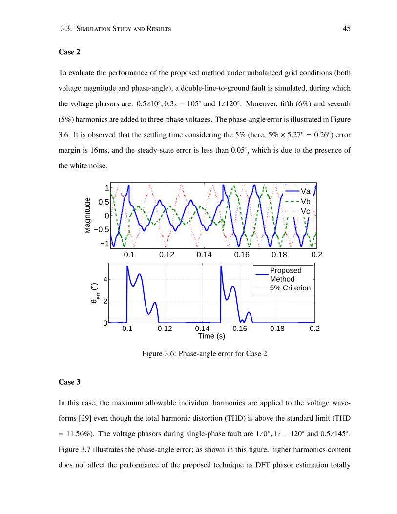
3.3. Simulation Study and Results 45
Case 2
To evaluate the performance of the proposed method under unbalanced grid conditions (both
voltage magnitude and phase-angle), a double-line-to-ground fault is simulated, during which
the voltage phasors are: 0.5∠10◦, 0.3∠ − 105◦ and 1∠120◦. Moreover, fifth (6%) and seventh
(5%) harmonics are added to three-phase voltages. The phase-angle error is illustrated in Figure
3.6. It is observed that the settling time considering the 5% (here, 5% × 5.27◦ = 0.26◦) error
margin is 16ms, and the steady-state error is less than 0.05◦, which is due to the presence of
the white noise.
0.1 0.12 0.14 0.16 0.18 0.2−1
−0.5
0
0.5
1
Mag
nitu
de
VaVbVc
0.1 0.12 0.14 0.16 0.18 0.20
2
4
Time (s)
θ err (
°)
ProposedMethod5% Criterion
Figure 3.6: Phase-angle error for Case 2
Case 3
In this case, the maximum allowable individual harmonics are applied to the voltage wave-
forms [29] even though the total harmonic distortion (THD) is above the standard limit (THD
= 11.56%). The voltage phasors during single-phase fault are 1∠0◦, 1∠ − 120◦ and 0.5∠145◦.
Figure 3.7 illustrates the phase-angle error; as shown in this figure, higher harmonics content
does not affect the performance of the proposed technique as DFT phasor estimation totally
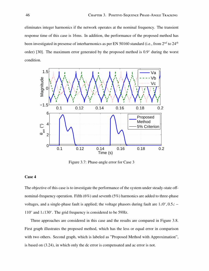
46 Chapter 3. Positive-Sequence Phase-Angle Tracking
eliminates integer harmonics if the network operates at the nominal frequency. The transient
response time of this case is 16ms. In addition, the performance of the proposed method has
been investigated in presense of interharmonics as per EN 50160 standard (i.e., from 2nd to 24th
order) [30]. The maximum error generated by the proposed method is 0.9◦ during the worst
condition.
0.1 0.12 0.14 0.16 0.18 0.2−1.5
0
1.5
Mag
nitu
de
VaVbVc
0.1 0.12 0.14 0.16 0.18 0.20
2
4
6
Time (s)
θ err (
°)
ProposedMethod5% Criterion
Figure 3.7: Phase-angle error for Case 3
Case 4
The objective of this case is to investigate the performance of the system under steady-state off-
nominal-frequency operation. Fifth (6%) and seventh (5%) harmonics are added to three-phase
voltages, and a single-phase fault is applied; the voltage phasors during fault are 1∠0◦, 0.5∠ −
110◦ and 1∠130◦. The grid frequency is considered to be 59Hz.
Three approaches are considered in this case and the results are compared in Figure 3.8.
First graph illustrates the proposed method, which has the less or equal error in comparison
with two others. Second graph, which is labeled as ”Proposed Method with Approximation”,
is based on (3.24), in which only the dc error is compensated and ac error is not.

3.3. Simulation Study and Results 47
0.1 0.12 0.14 0.16 0.18−1.2
0
1.2
Mag
nitu
de
VaVbVc
0.1 0.12 0.14 0.16 0.180
1
2
3
4
5
Time (s)
θ err (
°)
Proposed MethodProposed Method with ApproximationUncompensated Method5% Criterion
Figure 3.8: Phase-angle error for Case 4
Third graph, labeled as ”Uncompensated Method” shows the phase-angle error of the stan-
dard DFT without the proposed compensation method, which experiences high error values
due to the off-nominal frequency operation.
As it is discussed in Section 3.2.1, it is possible to ignore the negative-sequence component
to simplify the compensating equation and reduce the computational burden. As shown in
Figure 3.8, when the system is operating under a balanced condition, i.e. before t = 0.1s,
the phase-angle estimated by both the proposed method (3.23) and the proposed method with
approximation (3.24) are identical. Once phase-B and -C voltages drop to 0.5pu at t = 0.1s,
the negative-sequence voltage appears in the system; therefore, the phase-angle estimated by
the proposed method is more accurate than the one estimated by the approximated one. This
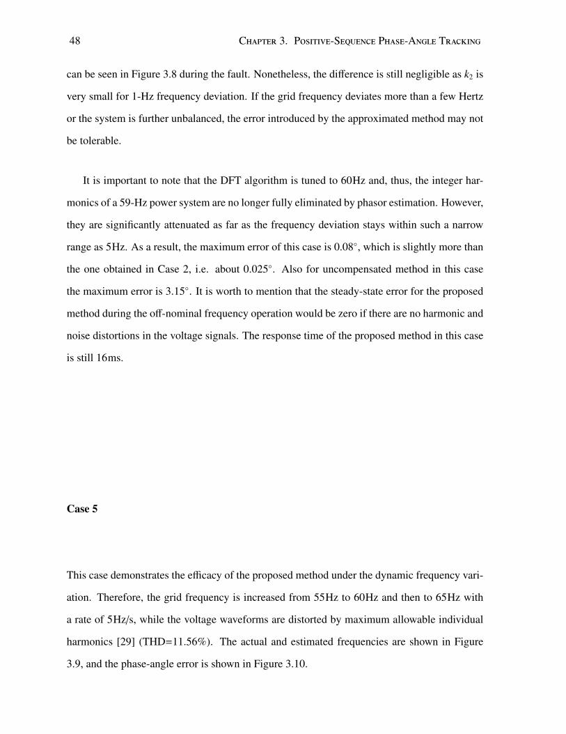
48 Chapter 3. Positive-Sequence Phase-Angle Tracking
can be seen in Figure 3.8 during the fault. Nonetheless, the difference is still negligible as k2 is
very small for 1-Hz frequency deviation. If the grid frequency deviates more than a few Hertz
or the system is further unbalanced, the error introduced by the approximated method may not
be tolerable.
It is important to note that the DFT algorithm is tuned to 60Hz and, thus, the integer har-
monics of a 59-Hz power system are no longer fully eliminated by phasor estimation. However,
they are significantly attenuated as far as the frequency deviation stays within such a narrow
range as 5Hz. As a result, the maximum error of this case is 0.08◦, which is slightly more than
the one obtained in Case 2, i.e. about 0.025◦. Also for uncompensated method in this case
the maximum error is 3.15◦. It is worth to mention that the steady-state error for the proposed
method during the off-nominal frequency operation would be zero if there are no harmonic and
noise distortions in the voltage signals. The response time of the proposed method in this case
is still 16ms.
Case 5
This case demonstrates the efficacy of the proposed method under the dynamic frequency vari-
ation. Therefore, the grid frequency is increased from 55Hz to 60Hz and then to 65Hz with
a rate of 5Hz/s, while the voltage waveforms are distorted by maximum allowable individual
harmonics [29] (THD=11.56%). The actual and estimated frequencies are shown in Figure
3.9, and the phase-angle error is shown in Figure 3.10.

3.3. Simulation Study and Results 49
0.5 0.51 0.52 0.53 0.54 0.55−1.5
0
1.7
Mag
nitu
de
VaVbVc
0 0.5 1 1.5 2 2.555
60
65
Time (s)
Fre
quen
cy (
Hz)
Actual FrequencyEstimated Frequency
Figure 3.9: Actual and estimated frequency for Case 5
0 0.5 1 1.5 2 2.5−15
0
15
Time (s)
θ err (
°)
Proposed MethodUncompensated Method
0.35°
Less than 0.1°
Figure 3.10: Phase-angle error for Case 5
Both figures show the effectiveness of the proposed method during off-nominal frequency
operation and dynamic frequency variation. As it can be observed, the phase-angle error
reaches the maximum transient value of 0.35◦, while it is less than 0.1◦ in steady-state con-
dition (with 5Hz frequency deviation). The maximum angle error in steady-state condition
is 14.8◦ for the ”Uncompensated Method”. It is worth to mention that the sensitivity of the
proposed method to sampling frequency is quite low. For instance, simulating the Case 5 with
sampling frequency of 2880Hz will generate the same results. This is due to the fact that

50 Chapter 3. Positive-Sequence Phase-Angle Tracking
changing the sampling frequency will affect the side lobes of DFT filter that belong to the
higher frequencies, which are removed by the anti-aliasing filter before application of the DFT.
3.4 Interharmonic test
To the best of the author’s knowledge, none of the state-of-the-art methods for PLL applications
have investigated the impact of interharmonics [4], [7]-[9], [21]. For instance, the test case
number 4 of [21] is based on the harmonic limits recommended by the IEC 61000-3-6 [29]
and only evaluates the integer harmonic distortion during the nominal frequency operation.
However, in Case 5 of this chapter, the proposed method is evaluated for off-nominal frequency
operation of 5Hz where the integer harmonics behave as interharmonics for the 60Hz DFT.
Figure 3.11: Interharmonic test with order 1.5 and 2% magnitude
Nevertheless, the performance of the proposed method is evaluated in the presence of in-
terharmonics as per EN50160 [30] standard, and the results are depicted in Figures 3.11-3.14.
Figure 3.12: Interharmonic test with order 2.5 and 5% magnitude
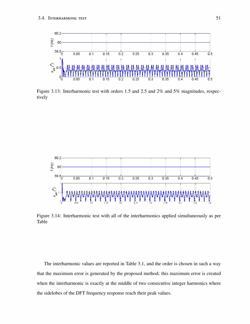
3.4. Interharmonic test 51
Figure 3.13: Interharmonic test with orders 1.5 and 2.5 and 2% and 5% magnitudes, respec-tively
Figure 3.14: Interharmonic test with all of the interharmonics applied simultaneously as perTable
The interharmonic values are reported in Table 3.1, and the order is chosen in such a way
that the maximum error is generated by the proposed method; this maximum error is created
when the interharmonic is exactly at the middle of two consecutive integer harmonics where
the sidelobes of the DFT frequency response reach their peak values.
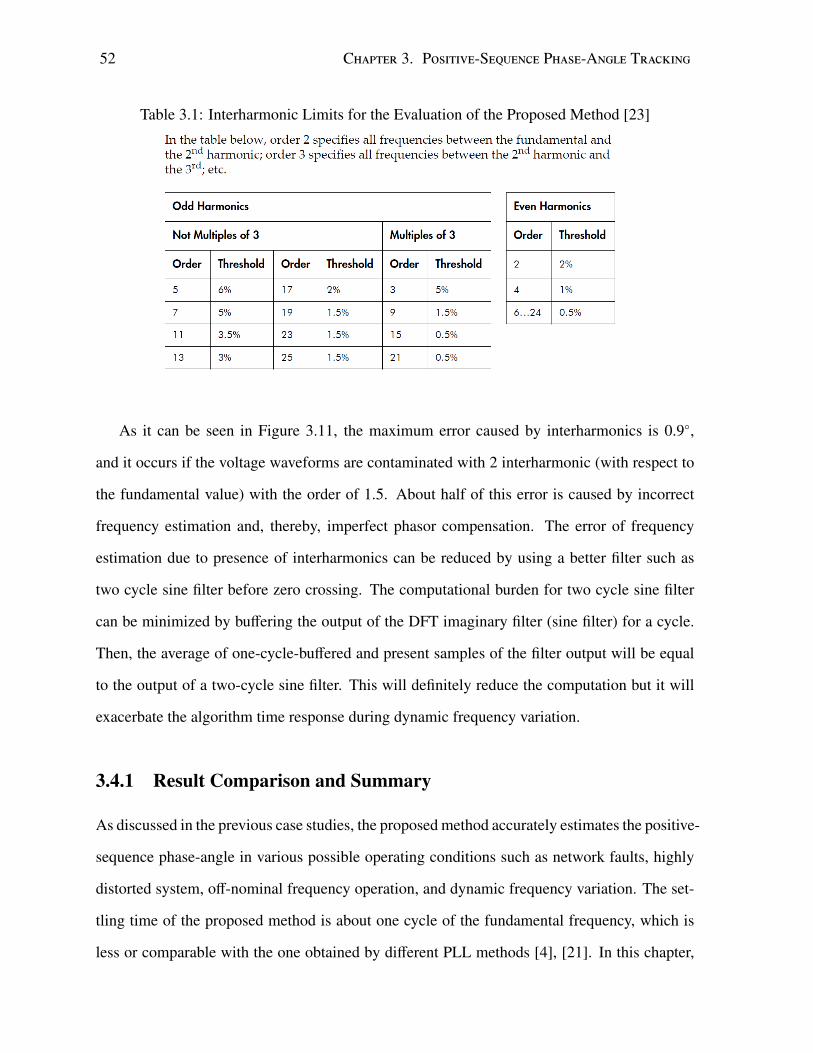
52 Chapter 3. Positive-Sequence Phase-Angle Tracking
Table 3.1: Interharmonic Limits for the Evaluation of the Proposed Method [23]
As it can be seen in Figure 3.11, the maximum error caused by interharmonics is 0.9◦,
and it occurs if the voltage waveforms are contaminated with 2 interharmonic (with respect to
the fundamental value) with the order of 1.5. About half of this error is caused by incorrect
frequency estimation and, thereby, imperfect phasor compensation. The error of frequency
estimation due to presence of interharmonics can be reduced by using a better filter such as
two cycle sine filter before zero crossing. The computational burden for two cycle sine filter
can be minimized by buffering the output of the DFT imaginary filter (sine filter) for a cycle.
Then, the average of one-cycle-buffered and present samples of the filter output will be equal
to the output of a two-cycle sine filter. This will definitely reduce the computation but it will
exacerbate the algorithm time response during dynamic frequency variation.
3.4.1 Result Comparison and Summary
As discussed in the previous case studies, the proposed method accurately estimates the positive-
sequence phase-angle in various possible operating conditions such as network faults, highly
distorted system, off-nominal frequency operation, and dynamic frequency variation. The set-
tling time of the proposed method is about one cycle of the fundamental frequency, which is
less or comparable with the one obtained by different PLL methods [4], [21]. In this chapter,
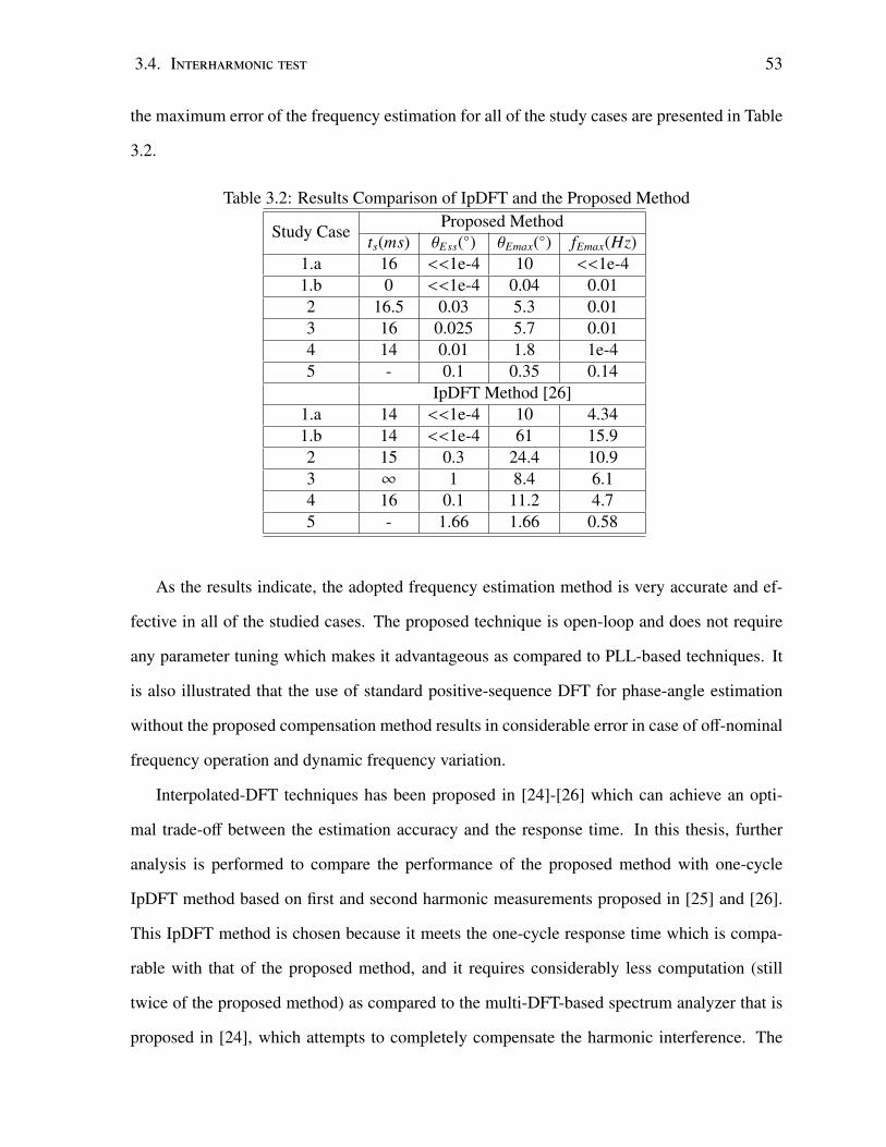
3.4. Interharmonic test 53
the maximum error of the frequency estimation for all of the study cases are presented in Table
3.2.
Table 3.2: Results Comparison of IpDFT and the Proposed Method
Study CaseProposed Method
ts(ms) θEss(◦) θEmax(◦) fEmax(Hz)1.a 16 <<1e-4 10 <<1e-41.b 0 <<1e-4 0.04 0.012 16.5 0.03 5.3 0.013 16 0.025 5.7 0.014 14 0.01 1.8 1e-45 - 0.1 0.35 0.14
IpDFT Method [26]1.a 14 <<1e-4 10 4.341.b 14 <<1e-4 61 15.92 15 0.3 24.4 10.93 ∞ 1 8.4 6.14 16 0.1 11.2 4.75 - 1.66 1.66 0.58
As the results indicate, the adopted frequency estimation method is very accurate and ef-
fective in all of the studied cases. The proposed technique is open-loop and does not require
any parameter tuning which makes it advantageous as compared to PLL-based techniques. It
is also illustrated that the use of standard positive-sequence DFT for phase-angle estimation
without the proposed compensation method results in considerable error in case of off-nominal
frequency operation and dynamic frequency variation.
Interpolated-DFT techniques has been proposed in [24]-[26] which can achieve an opti-
mal trade-off between the estimation accuracy and the response time. In this thesis, further
analysis is performed to compare the performance of the proposed method with one-cycle
IpDFT method based on first and second harmonic measurements proposed in [25] and [26].
This IpDFT method is chosen because it meets the one-cycle response time which is compa-
rable with that of the proposed method, and it requires considerably less computation (still
twice of the proposed method) as compared to the multi-DFT-based spectrum analyzer that is
proposed in [24], which attempts to completely compensate the harmonic interference. The

54 Chapter 3. Positive-Sequence Phase-Angle Tracking
comparison results are presented in Table 3.2. The parameters in this table are defined as:
ts: response time, θEss: positive-sequence phase-angle steady state error, θEmax: maximum
positive-sequence phase-angle error, and fEmax: maximum positive-sequence frequency esti-
mation error. As it is shown in this table, the proposed method offers comparable settling time
to the IpDFT method while it shows considerably smaller angle error both in transient (θEmax)
and steady state (θEss). This is mostly due to the fact that the proposed method benefits from an
accurate frequency estimation as compared to the IpDFT method. In the followings, the results
comparison is given between the proposed method and the IpDFT method presented in [26] for
the five aforementioned study cases in this chapter through Figures 3.15 to 3.20. The voltage
signals are generated as described in Section 3.3. The positive-sequence phasor is calculated
for the IpDFT method to compare the results with the proposed method which measures the
positive-sequence phase-angle. Furthermore, the average of the frequencies for three separate
phases is considered as the estimated frequency for the IpDFT method.

3.4. Interharmonic test 55
Figure 3.15: Results comparison for Case 1.a

56 Chapter 3. Positive-Sequence Phase-Angle Tracking
Figure 3.16: Results comparison for Case 1.b

3.4. Interharmonic test 57
Figure 3.17: Results comparison for Case 2
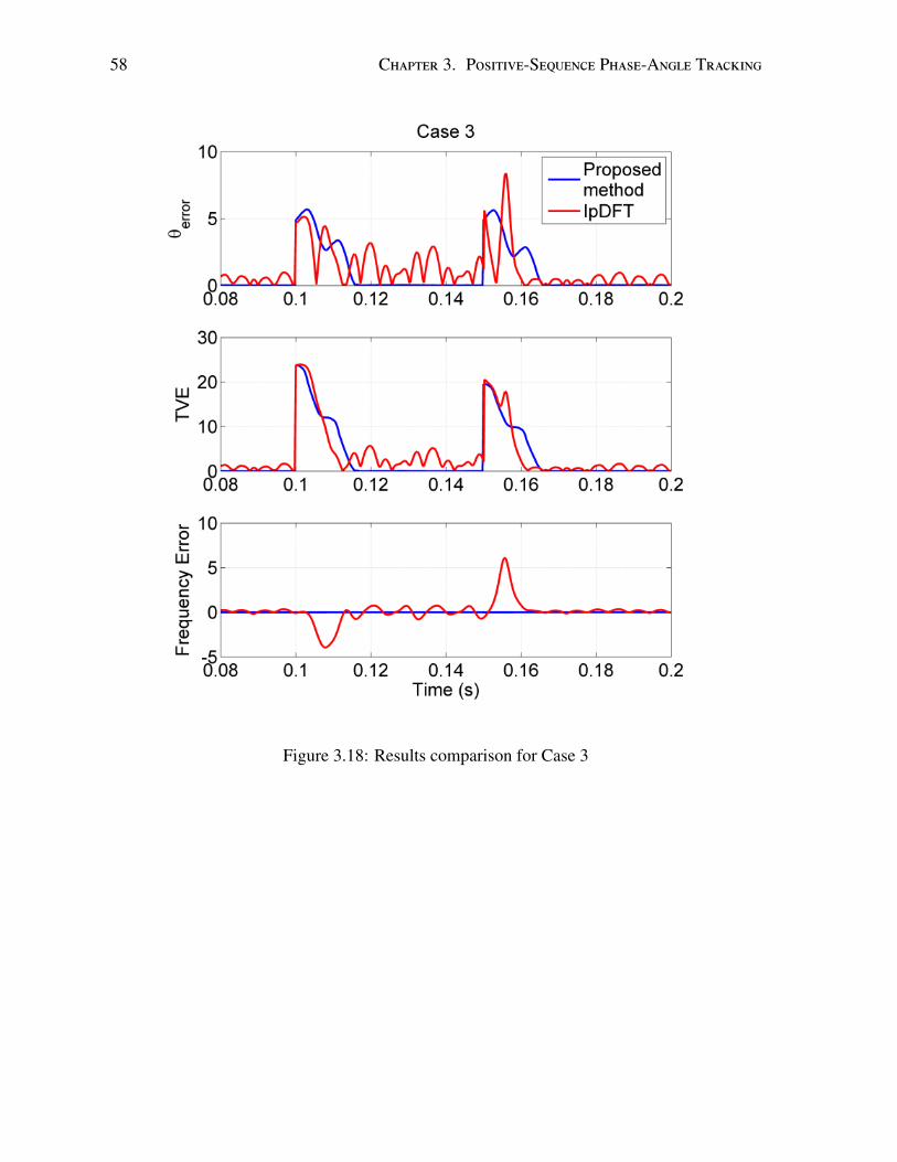
58 Chapter 3. Positive-Sequence Phase-Angle Tracking
Figure 3.18: Results comparison for Case 3
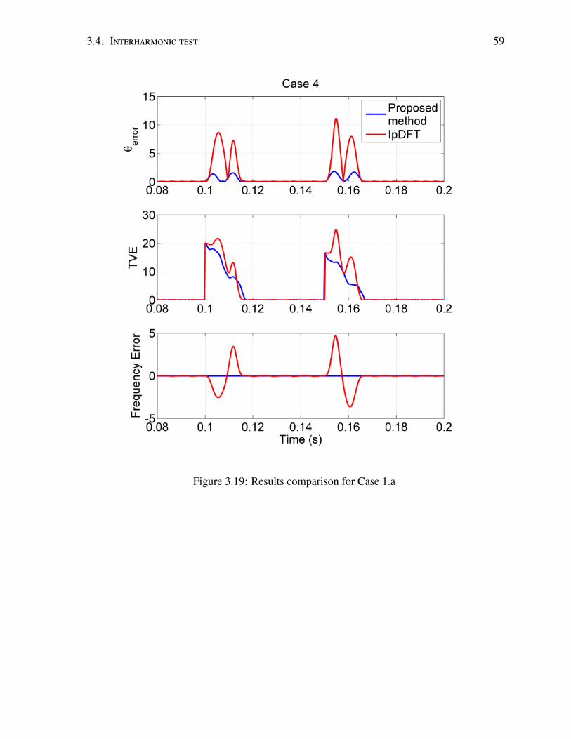
3.4. Interharmonic test 59
Figure 3.19: Results comparison for Case 1.a
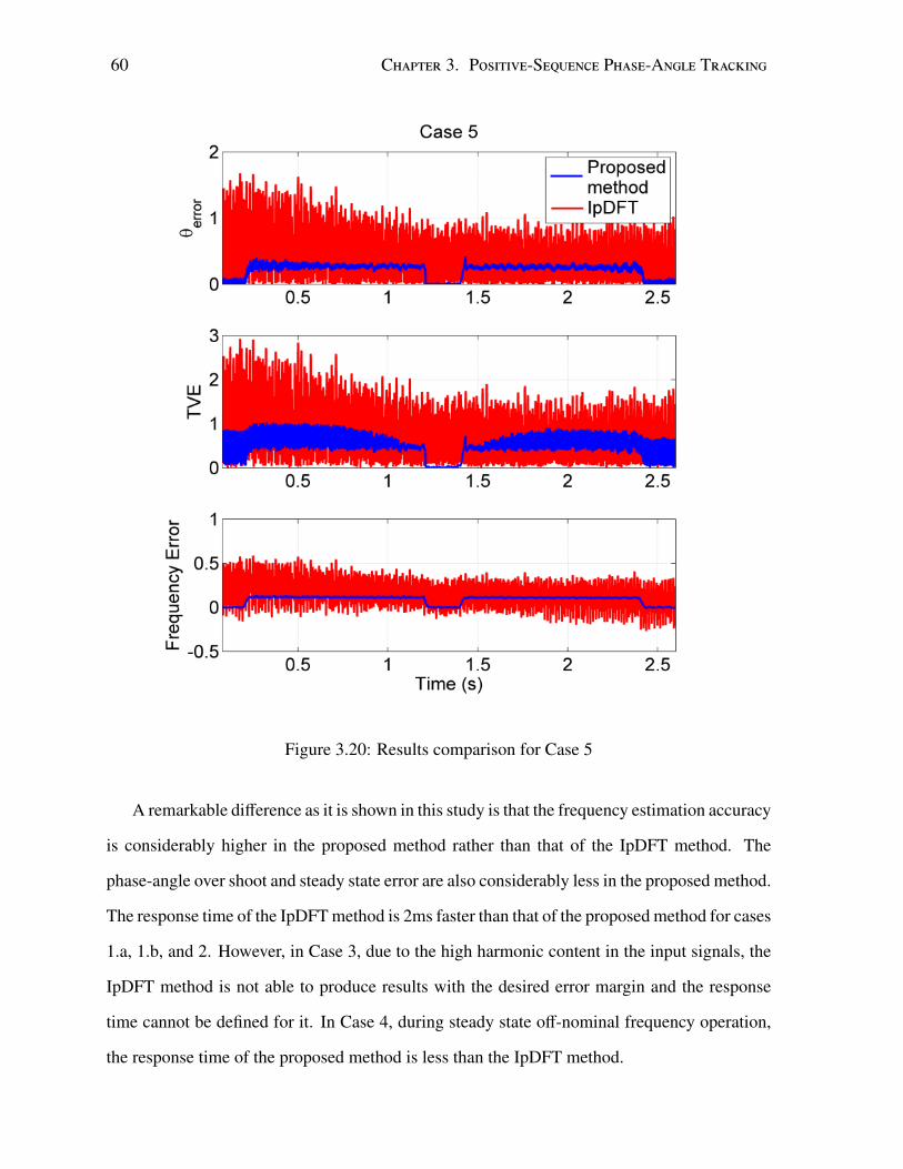
60 Chapter 3. Positive-Sequence Phase-Angle Tracking
Figure 3.20: Results comparison for Case 5
A remarkable difference as it is shown in this study is that the frequency estimation accuracy
is considerably higher in the proposed method rather than that of the IpDFT method. The
phase-angle over shoot and steady state error are also considerably less in the proposed method.
The response time of the IpDFT method is 2ms faster than that of the proposed method for cases
1.a, 1.b, and 2. However, in Case 3, due to the high harmonic content in the input signals, the
IpDFT method is not able to produce results with the desired error margin and the response
time cannot be defined for it. In Case 4, during steady state off-nominal frequency operation,
the response time of the proposed method is less than the IpDFT method.
3.5. Summary and Conclusion 61
3.5 Summary and Conclusion
A robust DFT-based phase-angle tracking method was proposed in this chapter for positive-
sequence phase-angle-tracking purposes in three-phase applications. It was shown that the
main advantage of this method is the accuracy and short transient response under distorted, un-
balanced, off-nominal frequency, and dynamic frequency variation conditions. The proposed
method has a simple digital open-loop structure and does not need application-specific tun-
ing (in contrary to closed-loop PLLs). The performance of the proposed method have been
evaluated through various extensive study cases including distorted signals with harmonics,
interharmonics, noise, unbalanced voltage operation, off-nominal frequency operation, and dy-
namic frequency variation; the results show that the proposed technique accurately tracks the
positive-sequence phase-angle with the maximum time response of one power system cycle,
during all possible abnormal grid conditions.

Chapter 4
Phase-Angle Tracking in
Single/Three-Phase Applications
4.1 Introduction
In the previous chapter, a robust positive-sequence phase-angle-tracking method was proposed
for three-phase applications. In this chapter, a phase-angle tracking method is proposed for
single-phase applications. The proposed method can be used for both voltage and current
signals, and also can be further extended to three-phase applications. In Section 4.2, the error in
the estimated-phasor by DFT in variable frequency environment is analytically calculated. The
adaptive window length is also considered for the DFT phasor-estimation. Then, the accurate
phasor and respectively, its phase-angle is calculated based on the estimated phasor by the DFT,
estimated frequency, and two proposed compensation coefficients. Since the compensation
coefficients and the adaptive window length are functions of the input signal’s frequency, a
robust zero-crossing-based frequency tracking system is also adopted for this purpose. It is
shown that the adopted frequency estimation losses accuracy when the window length of the
DFT filter is changed due to frequency variation. A new technique is presented to considerably
enhance the performance of the adopted frequency estimation technique while using adaptive
62

4.2. Proposed Algorithm 63
window length. In Section 3.3, four extensive case studies are conducted in the Matlab software
to evaluate the performance of the proposed method. Hardware implementation is done using a
digital signal processor and an arbitrary signal generator, i.e., specifically designed for testing
the proposed algorithm. The experimental results are compared with the simulation results and
it is shown that they are almost identical.
4.2 Proposed Algorithm
4.2.1 Accurate Phasor Measurement
To determine the DFT error for phasor estimation under off-nominal frequency operation, let us
consider the phasor of a voltage signal estimated by a full-cycle DFT. Equation (3.1) represents
a generic sinusoidal voltage signal in a discrete-time domain.
v[n] = Vm cos(2π fg
fsn + θ0
)(4.1)
where Vm is the signal magnitude, and θ0 denotes the angle at n = 0. The signal is sampled at
the constant sampling frequency of fs, and fg is the grid actual frequency. v[n] is the discrete
form of a continuous-time signal and n specifies the sample number.
According to the definition of full-cycle DFT, the fundamental-frequency phasor (V) of a
discrete voltage signal v[n] can be represented as
V =2N
N−1∑n=0
v[n]e− j 2πN n. (4.2)
In (4.2), N ∈ N is the DFT-window length and is chosen based on the grid frequency as given
in (4.3). In this equation, round(.) calculates the closest natural number of a real quantity.
N = round(fs
fg) (4.3)
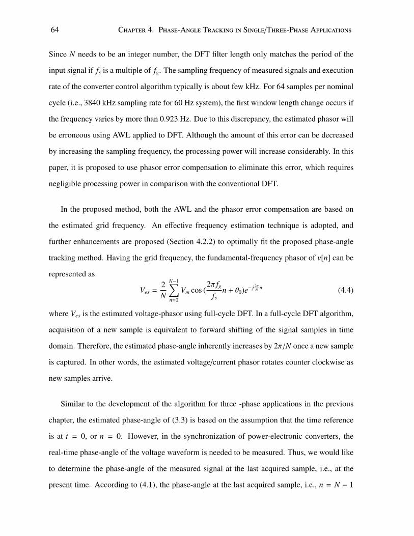
64 Chapter 4. Phase-Angle Tracking in Single/Three-Phase Applications
Since N needs to be an integer number, the DFT filter length only matches the period of the
input signal if fs is a multiple of fg. The sampling frequency of measured signals and execution
rate of the converter control algorithm typically is about few kHz. For 64 samples per nominal
cycle (i.e., 3840 kHz sampling rate for 60 Hz system), the first window length change occurs if
the frequency varies by more than 0.923 Hz. Due to this discrepancy, the estimated phasor will
be erroneous using AWL applied to DFT. Although the amount of this error can be decreased
by increasing the sampling frequency, the processing power will increase considerably. In this
paper, it is proposed to use phasor error compensation to eliminate this error, which requires
negligible processing power in comparison with the conventional DFT.
In the proposed method, both the AWL and the phasor error compensation are based on
the estimated grid frequency. An effective frequency estimation technique is adopted, and
further enhancements are proposed (Section 4.2.2) to optimally fit the proposed phase-angle
tracking method. Having the grid frequency, the fundamental-frequency phasor of v[n] can be
represented as
Ves =2N
N−1∑n=0
Vm cos (2π fg
fsn + θ0)e− j 2π
N n (4.4)
where Ves is the estimated voltage-phasor using full-cycle DFT. In a full-cycle DFT algorithm,
acquisition of a new sample is equivalent to forward shifting of the signal samples in time
domain. Therefore, the estimated phase-angle inherently increases by 2π/N once a new sample
is captured. In other words, the estimated voltage/current phasor rotates counter clockwise as
new samples arrive.
Similar to the development of the algorithm for three -phase applications in the previous
chapter, the estimated phase-angle of (3.3) is based on the assumption that the time reference
is at t = 0, or n = 0. However, in the synchronization of power-electronic converters, the
real-time phase-angle of the voltage waveform is needed to be measured. Thus, we would like
to determine the phase-angle of the measured signal at the last acquired sample, i.e., at the
present time. According to (4.1), the phase-angle at the last acquired sample, i.e., n = N − 1

4.2. Proposed Algorithm 65
can be expressed as
θN−1 = 2πfg
fs(N − 1) + θ0 (4.5)
where θN−1 is the phase-angle of the voltage signal considering the time of the last sample
acquisition as the reference time. Similarly, the phasor of the voltage signal considering the
last sample acquisition as the reference time can be calculated. This phasor is referred to as the
accurate phasor VAcc, and given by
VAcc = Vme j(2π
fgfs
(N−1)+θ0
). (4.6)
Since it is required to track the angle of the accurate phasor for phase-angle tracking appli-
cations, the estimated phasor in (4.4) is needed to be expressed in terms of VAcc. The mathe-
matical process is given below.
Ves =Vm
N
N−1∑n=0
e jθ0e( j2π fg
fsn)e− j 2π
N n +Vm
N
N−1∑n=0
e− jθ0e− j(2π fg
fsn)e− j 2π
N n
=VmN
e jθ0
N−1∑n=0
e j2πn(fgfs− 1
N ) +VmN
e− jθ0
N−1∑n=0
e− j2πn(fgfs
+ 1N )
=Vm
Ne jθ0
1 − e j2πN(fgfs− 1
N )
1 − e j2π(fgfs− 1
N )+
Vm
Ne jθ0
1 − e− j2πN(fgfs
+ 1N )
1 − e− j2π(fgfs
+ 1N ). (4.7)
By multiplying the equation (4.7) with and dividing it by VAcc and simplifying the terms, one
can get
Ves =VAcc
N
e− jπ fgN
fs
(e− j
π fgNfs − e j
π fgNfs
)e− j 2π
N
(e− j2π(
fgfs− 1
N )− 1
) +V∗Acc
N
e jπ fgN
fs
(e j
π fgNfs − e− j
π fgNfs
)e− j 2π
N
(e j2π(
fgfs
+ 1N )− 1
) (4.8)
=VAcc
Ne− j
π fgNfs
e− jπ fgN
fs −ejπ fgN
fs
e− j 2π
N e− jπ(fgfs− 1
N )(e− jπ(
fgfs− 1
N )− e jπ(
fgfs− 1
N ))
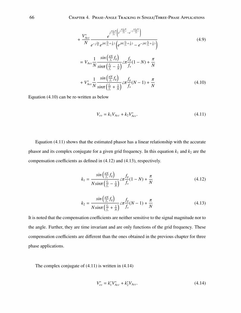
66 Chapter 4. Phase-Angle Tracking in Single/Three-Phase Applications
+V∗Acc
Ne
jπ fgN
fs
e jπ fgN
fs −e− j
π fgNfs
e− j 2π
N e jπ(fgfs
+ 1N )
(e jπ(
fgfs
+ 1N )− e− jπ(
fgfs
+ 1N )) (4.9)
= VAcc1N
sin(πNfs
fg
)sinπ
( fgfs− 1
N
)∠π fg
fs(1 − N) +
π
N
+ V∗Acc1N
sin(πNfs
fg
)sinπ
( fgfs
+ 1N
)∠π fg
fs(N − 1) +
π
N(4.10)
Equation (4.10) can be re-written as below
Ves = k1VAcc + k2V∗Acc. (4.11)
Equation (4.11) shows that the estimated phasor has a linear relationship with the accurate
phasor and its complex conjugate for a given grid frequency. In this equation k1 and k2 are the
compensation coefficients as defined in (4.12) and (4.13), respectively.
k1 =sin
(πNfs
fg
)Nsinπ
( fgfs− 1
N
)∠π fg
fs(1 − N) +
π
N(4.12)
k2 =sin
(πNfs
fg
)Nsinπ
( fgfs
+ 1N
)∠π fg
fs(N − 1) +
π
N(4.13)
It is noted that the compensation coefficients are neither sensitive to the signal magnitude nor to
the angle. Further, they are time invariant and are only functions of the grid frequency. These
compensation coefficients are different than the ones obtained in the previous chapter for three
phase applications.
The complex conjugate of (4.11) is written in (4.14)
V∗es = k∗1V∗Acc + k∗2VAcc. (4.14)
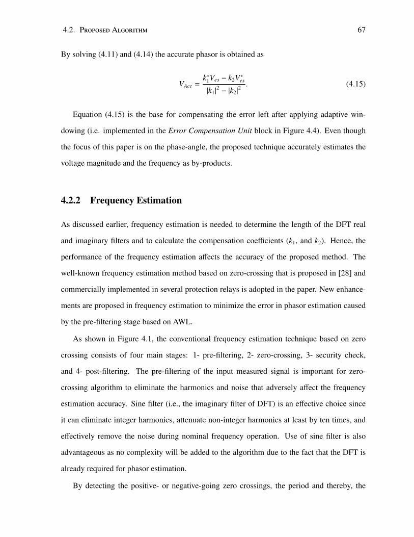
4.2. Proposed Algorithm 67
By solving (4.11) and (4.14) the accurate phasor is obtained as
VAcc =k∗1Ves − k2V∗es
|k1|2− |k2|
2 . (4.15)
Equation (4.15) is the base for compensating the error left after applying adaptive win-
dowing (i.e. implemented in the Error Compensation Unit block in Figure 4.4). Even though
the focus of this paper is on the phase-angle, the proposed technique accurately estimates the
voltage magnitude and the frequency as by-products.
4.2.2 Frequency Estimation
As discussed earlier, frequency estimation is needed to determine the length of the DFT real
and imaginary filters and to calculate the compensation coefficients (k1, and k2). Hence, the
performance of the frequency estimation affects the accuracy of the proposed method. The
well-known frequency estimation method based on zero-crossing that is proposed in [28] and
commercially implemented in several protection relays is adopted in the paper. New enhance-
ments are proposed in frequency estimation to minimize the error in phasor estimation caused
by the pre-filtering stage based on AWL.
As shown in Figure 4.1, the conventional frequency estimation technique based on zero
crossing consists of four main stages: 1- pre-filtering, 2- zero-crossing, 3- security check,
and 4- post-filtering. The pre-filtering of the input measured signal is important for zero-
crossing algorithm to eliminate the harmonics and noise that adversely affect the frequency
estimation accuracy. Sine filter (i.e., the imaginary filter of DFT) is an effective choice since
it can eliminate integer harmonics, attenuate non-integer harmonics at least by ten times, and
effectively remove the noise during nominal frequency operation. Use of sine filter is also
advantageous as no complexity will be added to the algorithm due to the fact that the DFT is
already required for phasor estimation.
By detecting the positive- or negative-going zero crossings, the period and thereby, the

68 Chapter 4. Phase-Angle Tracking in Single/Three-Phase Applications
frequency of the signal is calculated. Both positive- and negative-going zero crossings are
considered in the proposed method to obtain faster response from the frequency estimation.
The frequency that is calculated by the zero-crossing is called raw frequency because it may
not be accurate as a result of abnormal power-system grid conditions (e.g. transients, off-
nominal frequency operation, and faults). To eliminate the defective estimations of the raw
frequency, security check is applied as follows. First and second derivatives of raw frequency
is checked against appropriate thresholds (20Hz/s, and 600Hz/s2 in this paper, respectively).
These thresholds can be adjusted based on the system inertia to improve the performance if
significantly higher or lower rate-of-change-of-frequency is expected. If the first and second
derivatives are within the thresholds, the estimated raw frequency is passed to the fourth stage
where the raw frequency is applied to a low-pass infinite impulse response (IIR) filter to deter-
mine the new estimated frequency. Otherwise, the estimated frequency will not be updated by
fraw and its value from previous sample is kept. The IIR filter such as the one recommended
in [33] and given in (4.16) is required to further attenuate the impact of harmonics if grid
frequency deviates from its nominal value.
f [n] =78
f [n − 1] +18
fraw[n] (4.16)
where f [n] denotes the estimated frequency after post-filtering, and fraw[n] is the calculated
raw frequency at the real time.
As mentioned earlier and suggested in [33], an effective pre-filtering can be obtained if the
output of the DFT imaginary filter is used for the frequency estimation. However, by using
AWL in the DFT structure, during dynamic frequency operation, the DFT filter length may
change as grid frequency varies. This leads to a sudden jump in the filtered signal at each win-
dow length change which considerably affects the accuracy of the frequency estimation. Figure
4.2, dashed-line signal, shows that the output of the DFT imaginary filter suddenly changes at
t = 0.434s once the window length is changed during dynamic frequency variation. Figure 4.3
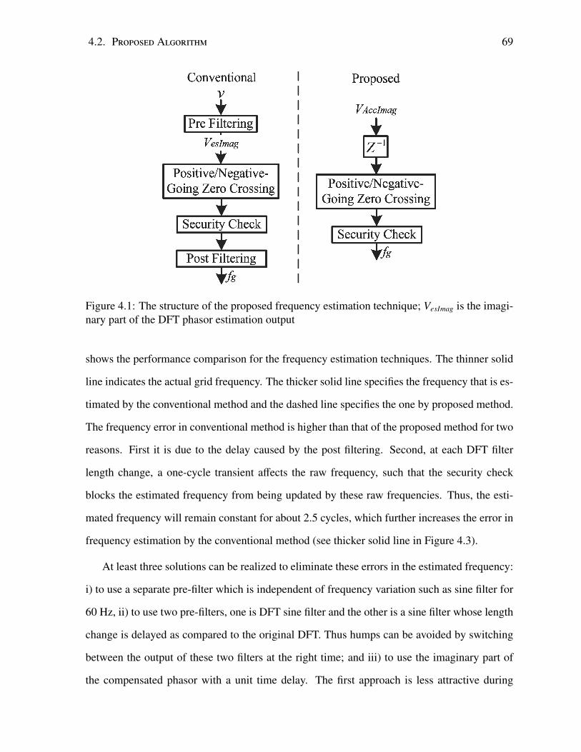
4.2. Proposed Algorithm 69
Figure 4.1: The structure of the proposed frequency estimation technique; VesImag is the imagi-nary part of the DFT phasor estimation output
shows the performance comparison for the frequency estimation techniques. The thinner solid
line indicates the actual grid frequency. The thicker solid line specifies the frequency that is es-
timated by the conventional method and the dashed line specifies the one by proposed method.
The frequency error in conventional method is higher than that of the proposed method for two
reasons. First it is due to the delay caused by the post filtering. Second, at each DFT filter
length change, a one-cycle transient affects the raw frequency, such that the security check
blocks the estimated frequency from being updated by these raw frequencies. Thus, the esti-
mated frequency will remain constant for about 2.5 cycles, which further increases the error in
frequency estimation by the conventional method (see thicker solid line in Figure 4.3).
At least three solutions can be realized to eliminate these errors in the estimated frequency:
i) to use a separate pre-filter which is independent of frequency variation such as sine filter for
60 Hz, ii) to use two pre-filters, one is DFT sine filter and the other is a sine filter whose length
change is delayed as compared to the original DFT. Thus humps can be avoided by switching
between the output of these two filters at the right time; and iii) to use the imaginary part of
the compensated phasor with a unit time delay. The first approach is less attractive during

70 Chapter 4. Phase-Angle Tracking in Single/Three-Phase Applications
large frequency variations as harmonics can not be effectively filtered. The seconds technique
requires more processing power. The third technique is recommended in this paper since it
presents almost the same results as (ii) without adding any complexity and processing demand
to the algorithm. Moreover, the pre-filter in this case is adaptive to the grid frequency and thus,
it can effectively attenuate harmonics even during off-nominal frequency operation.
In summary, it is proposed to use the imaginary part of the calculated accurate phasor (see
VAccImag in Figure 4.1). In this case, transients caused by the DFT window length change will
not affect the VAccImag because the corresponding phase-angle jump will be inherently compen-
sated through the compensation coefficients. By choosing VAccImag as the frequency estimation
input, the loop that is created between the phasor compensation and the frequency estimation
can be eliminated by using a unit delay in discrete domain (see z−1 block in Figure 4.4). This
one-sample-long delay does not have a considerable effect on the frequency estimation be-
cause, first, it is much less than the frequency estimation update rate, i.e., half a power-system
cycle, and second, power system frequency does not deviate considerably within one sample.
0.43 0.435 0.44 0.445−1
−0.5
0
0.5
1
Time (s)
Mag
nitu
de (
pu)
VAccImag
VesImag
DFT filter−lengthchange
Zoomed
Figure 4.2: The phase-angle jump in the VesImag caused by the DFT filter length change incomparison to VAccImag
To evaluate the performance of the conventional and proposed techniques, a study case is
conducted as follows. The grid frequency is dynamically changed from 55 to 65Hz with a
rate of change of frequency of 5Hz/s. The input signal is contaminated with noise and worst

4.3. Simulation Study and Results 71
case of harmonic distortion including 2nd to 50th order as per [29]. The performance of both
techniques are depicted versus the actual frequency. As it can be seen, there are small humps
in the estimated frequency by conventional method. These humps are one-cycle in length, and
indicate the instant that the DFT window length (N) is changed.
0.2 0.3 0.4 0.5 0.6 0.7 0.8 0.955
56
57
58
Time (s)
Fre
quen
cy (
Hz)
Actual FrequencyProposed MethodConventional Method
fraw
blocked by
security check
Figure 4.3: Performance comparison of the conventional and proposed frequency estimationtechniques
When the input signal drops down to zero during temporary close-in faults, it is also pro-
posed to generate fictional phase-angle based on the latest valid estimated frequency and phase
angle until the input signal is recovered (within a predefined number of cycles). The afore-
mentioned functions in this subsection are implemented in the Frequency Estimation block in
Figure 4.4.
4.3 Simulation Study and Results
4.3.1 Simulation Settings
Matlab is used to evaluate the performance of the proposed method for different operational
conditions including harmonic interference, noise distortion, voltage dip, phase-angle jump,
off-nominal frequency, dynamic-frequency deviation, and close-in faults. Figure 4.4 illustrates
the block diagram of the proposed method implemented in Matlab. The test signals are first
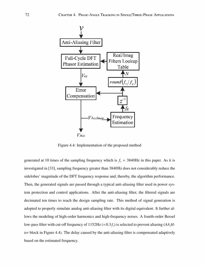
72 Chapter 4. Phase-Angle Tracking in Single/Three-Phase Applications
Figure 4.4: Implementation of the proposed method
generated at 10 times of the sampling frequency which is fs = 3840Hz in this paper. As it is
investigated in [33], sampling frequency greater than 3840Hz does not considerably reduce the
sidelobes’ magnitude of the DFT frequency response and, thereby, the algorithm performance.
Then, the generated signals are passed through a typical anti-aliasing filter used in power sys-
tem protection and control applications. After the anti-aliasing filter, the filtered signals are
decimated ten times to reach the design sampling rate. This method of signal generation is
adopted to properly simulate analog anti-aliasing filter with its digital equivalent. It further al-
lows the modeling of high-order harmonics and high-frequency noises. A fourth-order Bessel
low-pass filter with cut-off frequency of 1152Hz (=0.3 fs) is selected to prevent aliasing (AA fil-
ter block in Figure 4.4). The delay caused by the anti-aliasing filter is compensated adaptively
based on the estimated frequency.
4.3. Simulation Study and Results 73
A full-cycle DFT algorithm with variable window length and phasor compensation is em-
ployed to estimate the phasor of the input voltage/current signal. The grid frequency fg is
estimated using the zero-crossing technique as described in Section 4.2.2. Having fg, the error
compensation unit calculates k1 and k2, and thereby VAcc. The entire process of angle estimation
is executed at the sampling frequency, i.e., 3840Hz.
The major computational burden of the proposed method is as follows: i) Full-cycle DFT
requires 2 × N multiplications and N summation at each data sample acquisition; ii) the fre-
quency estimation requires 13 multiplications, and 8 summations; and iii) calculation of com-
pensation coefficients requires 11 multiplications and 7 summations. Considering the fact that
the frequency estimation and calculation of compensation coefficients are executed every half
of a power system cycle, the proposed algorithm requires 0.2% and 0.25% increase in multi-
plications and summations of the conventional DFT, respectively. In order to further decrease
the computational burden of the entire algorithm, it is possible to buffer the samples at the
sampling rate and perform the phasor estimation at every few samples, e.g., 4 samples, to
significantly reduce the computational burden. In such a case, if the control system requires
higher resolution, the phase-angle can be linearly extrapolated using the latest two consecutive
estimations.
4.3.2 Study Cases
The phase angle of measured waveform from field or electromagnetic transient simulations are
not known in advance. Hence, there will not be a 100% accurate reference signal available for
result comparison and error measurement. As adopted in the previous studies such as [4], [8],
[21], and [33], to accurately estimate the performance of the proposed method, a pre-known
phase-angle is first generated. Then, voltage waveform and its harmonics are calculated as a
function of the pre-known phase-angle. Various study cases have been generated combining
the voltage waveform, its harmonics and noise during various events. Finally, the estimated
angle is compared against the pre-known phase angle to determine the error.
74 Chapter 4. Phase-Angle Tracking in Single/Three-Phase Applications
Four cases are studied to demonstrate the effectiveness of the proposed method in various
grid conditions. In all cases white noise with signal-to-noise ratio of 40dB is applied to the
voltage signal to simulate the worst conditions of noise distortion. The pre-fault voltage phasor,
i.e. the normal grid operating condition, is 1∠0◦. To determine the settling time for Case 1,
5% of the applied phase-angle jump is considered as the error band. The settling time (ts) is
determined when the phase-angle error enters and remains inside the error band.
Case 1
In this case, the performance of the proposed method is evaluated in response to a 10◦ phase-
angle jump and 50% voltage dip. Worst conditions of noise and maximum allowable individual
harmonic distortion that is applied simultaneously from the 2nd to 50th order are also consid-
ered. The per-unit voltage during this incident is changed to 0.5∠10◦. Figure 4.5 depicts the
absolute phase-angle error for this case considering three different approaches. First approach
is the DFT with AWL and without applying phasor compensation. In the second approach,
the AWL is disabled and phasor compensation is applied. The third approach is the proposed
method enabling both AWL and the phasor compensation. As it is shown in Figure 4.5 when
the grid frequency is equal to its nominal value, there is no differences between these three
approaches. However, in the following study cases, it is shown that the performances of the
first and second approaches are vulnerable to off-nominal and/or dynamic frequency operation.
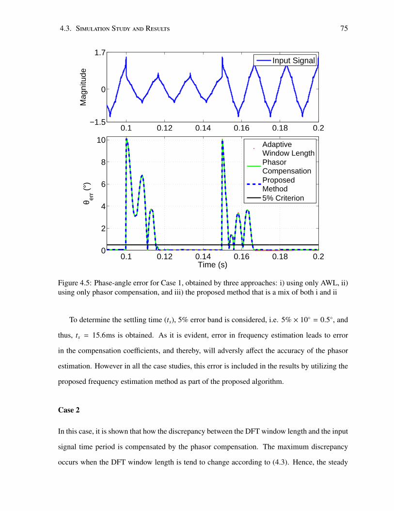
4.3. Simulation Study and Results 75
0.1 0.12 0.14 0.16 0.18 0.2−1.5
0
1.7
Mag
nitu
de
Input Signal
0.1 0.12 0.14 0.16 0.18 0.20
2
4
6
8
10
Time (s)
θ err (
°)
AdaptiveWindow LengthPhasorCompensationProposedMethod5% Criterion
Figure 4.5: Phase-angle error for Case 1, obtained by three approaches: i) using only AWL, ii)using only phasor compensation, and iii) the proposed method that is a mix of both i and ii
To determine the settling time (ts), 5% error band is considered, i.e. 5% × 10◦ = 0.5◦, and
thus, ts = 15.6ms is obtained. As it is evident, error in frequency estimation leads to error
in the compensation coefficients, and thereby, will adversly affect the accuracy of the phasor
estimation. However in all the case studies, this error is included in the results by utilizing the
proposed frequency estimation method as part of the proposed algorithm.
Case 2
In this case, it is shown that how the discrepancy between the DFT window length and the input
signal time period is compensated by the phasor compensation. The maximum discrepancy
occurs when the DFT window length is tend to change according to (4.3). Hence, the steady

76 Chapter 4. Phase-Angle Tracking in Single/Three-Phase Applications
state off-nominal frequency of 59.54Hz is chosen to simulate the maximum discrepancy in this
case. Worst conditions of noise and harmonics are also considered as discussed in Case 1.
Simulation result is depicted in Figure 4.6.
0.1 0.12 0.14 0.16 0.18
−1
0
1
Mag
nitu
de
Input Signal
0.1 0.12 0.14 0.16 0.180
0.5
1
1.5
Time (s)
θ err (
°)
Adaptive Window LengthPhasor CompensationProposed Method
Figure 4.6: Phase-angle error for Case 2
The dotted curve shows the amount of error caused by the discrepancy between the DFT
window length and the input signal’s time period. For the proposed method, the steady-state
error is less than 0.04◦, which is due to the presence of white noise and harmonics.
Case 3
In this study case, the performance of the proposed method is evaluated during a dynamic
frequency operation. The grid frequency is changed from 55 to 65Hz with a rate of change of
frequency of 5 Hz/s. The input signal is distorted with noise and harmonics similar to Case 1.

4.3. Simulation Study and Results 77
Figure 4.7: Phase-angle error for Case 3
Figure 4.7(a)shows the input signal. In figure 4.7(b) the simulation result is given while
phasor compensation is disabled. This figure denotes that for some certain points, the DFT
window length matches the period of the input signal and phase-angle error is zero. However

78 Chapter 4. Phase-Angle Tracking in Single/Three-Phase Applications
in this case, the maximum error is (1.85◦) with AWL. In Figure 4.7(c), the phasor compensation
is enabled and the AWL is disable to only evaluate the efficacy of the phasor compensation.
In this case the maximum error in the phase-angle estimation is less than 0.9◦. Figure 4.7(d)
depicts the result obtained by the proposed method. Error in phase-angle will further decrease
to less than 0.3◦ because of using the combination of phasor compensation and AWL. It is noted
that the error caused by the harmonic distortion during off-nominal frequency of operation
effectively decreases using the AWL. This is because the DFT filters are tuned with respect to
the grid frequency so that they can effectively attenuate the harmonics even during off-nominal
frequency operation.
Case 4
As mentioned earlier, to further improve the proposed method, a memory is embedded in
the algorithm to protect the phase-angle tracking even during the temporary close-in faults.
Therefore, in case the magnitude of the input signal drops down below a very small value, the
phase angle will be generated based on the last valid estimated frequency for a pre-determined
number of cycles. The phase-angle will be extrapolated using two corresponding samples of
phase-angle from two cycles back. Two cycles are chosen to make sure that at least one cycle
of the DFT transient period is passed after the detection of the close-in fault.
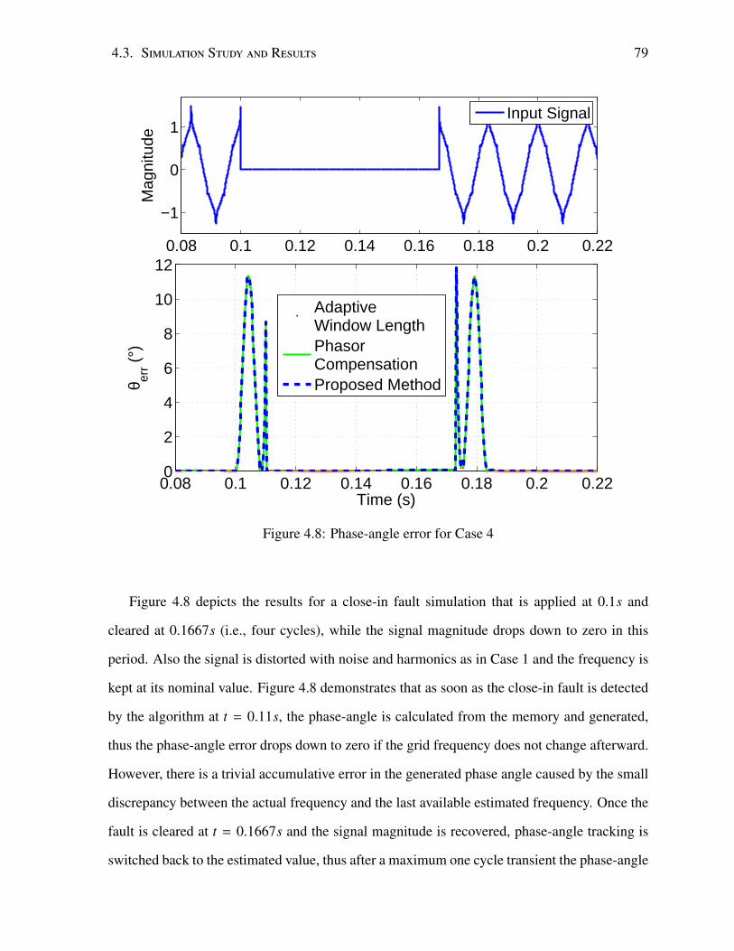
4.3. Simulation Study and Results 79
0.08 0.1 0.12 0.14 0.16 0.18 0.2 0.22
−1
0
1M
agni
tude
Input Signal
0.08 0.1 0.12 0.14 0.16 0.18 0.2 0.220
2
4
6
8
10
12
Time (s)
θ err (
°)
AdaptiveWindow LengthPhasorCompensationProposed Method
Figure 4.8: Phase-angle error for Case 4
Figure 4.8 depicts the results for a close-in fault simulation that is applied at 0.1s and
cleared at 0.1667s (i.e., four cycles), while the signal magnitude drops down to zero in this
period. Also the signal is distorted with noise and harmonics as in Case 1 and the frequency is
kept at its nominal value. Figure 4.8 demonstrates that as soon as the close-in fault is detected
by the algorithm at t = 0.11s, the phase-angle is calculated from the memory and generated,
thus the phase-angle error drops down to zero if the grid frequency does not change afterward.
However, there is a trivial accumulative error in the generated phase angle caused by the small
discrepancy between the actual frequency and the last available estimated frequency. Once the
fault is cleared at t = 0.1667s and the signal magnitude is recovered, phase-angle tracking is
switched back to the estimated value, thus after a maximum one cycle transient the phase-angle

80 Chapter 4. Phase-Angle Tracking in Single/Three-Phase Applications
error drops down to almost zero.
4.4 Hardware Implementation and Test Results
4.4.1 Test Setup Specifications
The proposed algorithm is implemented in a Datatranslation real-time DSP data acquisition
module (DT9842), which uses an embedded TMS320C6713 300MHz processor. This module
has 8 A/D inputs and 2 D/A outputs both supporting ±10 volts range. The proposed algorithm
is implemented in C programming language using Code Composer Studio software. The gen-
erated signals as described in Section 3.3 are used to evaluate the performance of the hardware
implementation through the same four study cases described in Section 4.3.
To playback these signals, an arbitrary waveform generator is implemented using Matlab
xPC target equipped with General Standards PCI-ADADIO data acquisition board. Signals are
first generated and then played back through this system to an A/D input of the DSP module
and then processed within the proposed algorithm. Thereafter, the estimated phase-angle is ac-
quired from the D/A output of the DSP through the ADADIO board. Furthermore, to precisely
synchronize the DSP module with the arbitrary waveform generator, an external clock is gen-
erated by the waveform generator and fed to the DSP module (see Figure 4.9). A forth-order
active Bessel filter is used as the input anti-aliasing filter. This filter is designed using MF10
chips and tuned to have a cut-off frequency of 1.1kHz. The frequency response of this filter
closely complies with that of the anti-aliasing filter used in the simulation studies.
4.4.2 Test Results
The same signals that are generated for simulation studies are used in this subsection as input
signals for the hardware tests. The same four study cases as in Subsection 4.3.2 are tested
here so that the results can be compared with that of the simulation studies. Figs. 4.10 to 4.13

4.4. Hardware Implementation and Test Results 81
show the comparison results. As it is shown, the experimental results are almost identical to
the simulation results. The only difference is the level of noise that is more dominant in the
hardware implementation. This high frequency noise is due to the imperfections in A/D and
D/A conversions in the DSP module and data acquisition system.
Figure 4.9: The configuration of the experimental implementation
0.1 0.12 0.14 0.16 0.18 0.20
5
10
Time (s)
θ err (
°)
Experimental ResultSimulation Result5% Criterion
Figure 4.10: Phase-angle error obtained by the hardware implementation for Case 1
0.1 0.12 0.14 0.16 0.180
0.1
0.2
0.3
Time (s)
θ err (
°)
Experimental Result Simulation Result
Figure 4.11: Phase-angle error obtained by the hardware implementation for Case 2
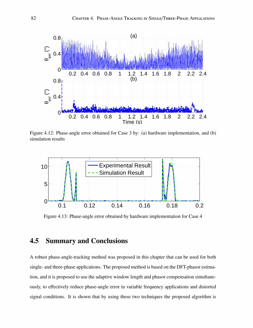
82 Chapter 4. Phase-Angle Tracking in Single/Three-Phase Applications
0.2 0.4 0.6 0.8 1 1.2 1.4 1.6 1.8 2 2.2 2.40
0.4
0.8
Time (s)
θ err (
°)
0.2 0.4 0.6 0.8 1 1.2 1.4 1.6 1.8 2 2.2 2.40
0.4
0.8
θ err (
°)
(a)
(b)
Figure 4.12: Phase-angle error obtained for Case 3 by: (a) hardware implementation, and (b)simulation results
0.1 0.12 0.14 0.16 0.18 0.20
5
10
Experimental ResultSimulation Result
Figure 4.13: Phase-angle error obtained by hardware implementation for Case 4
4.5 Summary and Conclusions
A robust phase-angle-tracking method was proposed in this chapter that can be used for both
single- and three-phase applications. The proposed method is based on the DFT-phasor estima-
tion, and it is proposed to use the adaptive window length and phasor compensation simultane-
ously, to effectively reduce phase-angle error in variable frequency applications and distorted
signal conditions. It is shown that by using these two techniques the proposed algorithm is
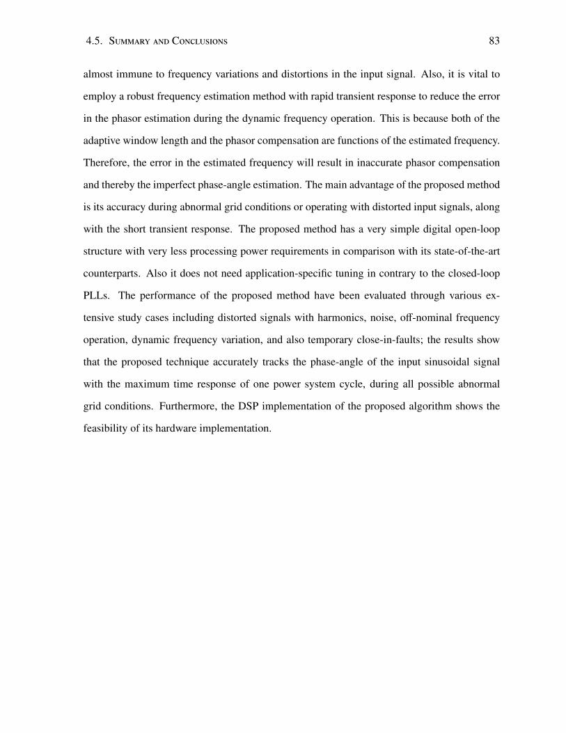
4.5. Summary and Conclusions 83
almost immune to frequency variations and distortions in the input signal. Also, it is vital to
employ a robust frequency estimation method with rapid transient response to reduce the error
in the phasor estimation during the dynamic frequency operation. This is because both of the
adaptive window length and the phasor compensation are functions of the estimated frequency.
Therefore, the error in the estimated frequency will result in inaccurate phasor compensation
and thereby the imperfect phase-angle estimation. The main advantage of the proposed method
is its accuracy during abnormal grid conditions or operating with distorted input signals, along
with the short transient response. The proposed method has a very simple digital open-loop
structure with very less processing power requirements in comparison with its state-of-the-art
counterparts. Also it does not need application-specific tuning in contrary to the closed-loop
PLLs. The performance of the proposed method have been evaluated through various ex-
tensive study cases including distorted signals with harmonics, noise, off-nominal frequency
operation, dynamic frequency variation, and also temporary close-in-faults; the results show
that the proposed technique accurately tracks the phase-angle of the input sinusoidal signal
with the maximum time response of one power system cycle, during all possible abnormal
grid conditions. Furthermore, the DSP implementation of the proposed algorithm shows the
feasibility of its hardware implementation.

Chapter 5
Summary and Conclusion
5.1 Summary
The presented thesis consists of five chapters. In the first chapter, an introduction to the control
systems of power-electronic converters that are employed in EC-DERs were presented. The
importance of the dq-frame controller for the EC-DERs and its need for a robust and accurate
phase-angle-tracking system were illustrated. Then, the available methods for phase-angle
tracking purposes and their specifications were thoroughly discussed along with the literature
survey. Thereafter, the research objectives were defined such that to introduce a new phase-
angle-tracking method with superior performance and fast time response for three-phase and
single phase applications. Finally, the thesis contributions and outline were presented.
In Chapter 2, the fundamentals of DFT-based phasor-estimation technique were presented.
First, the concept of phasor and windowing were introduced to show that how a phasor-
estimation technique can be employed to extract the phasors of time-variant power system sig-
nals. Then, the effect of frequency variation on DFT phasor estimation was investigated. It was
also shown that the DFT phasor-estimation technique is not immune to frequency variations
by itself and possible solutions were introduced to make the DFT adaptive to the frequency
variations. Finally, a summary for this chapter was provided.
84
5.1. Summary 85
In Chapter 3, a new method was proposed for positive-sequence phase-angle-tracking in
three-phase applications. First, a brief introduction was given and then, the error in phasor
estimation caused by the off-nominal frequency operation was analytically calculated. After-
wards, the accurate phasor was defined such that to present the magnitude and phase angle
of the input signal’s at the real time. Then, two compensation coefficients were proposed to
correct the estimated phasor by the DFT to obtain the accurate phasor. Approximations for
the compensation coefficients were developed to further reduce the required processing power
in practical applications. Since the obtained compensation coefficients were a function of the
input signals frequency, a zero-crossing based frequency estimation technique was adopted
and further adjusted to be used as part of the proposed method. Then, the proposed method
was simulated using Matlab and its performance was evaluated through five extensive study
cases, through which almost all of the possible abnormal grid conditions were covered. Fi-
nally, the results obtained by the proposed method were compared with that of the state-of-the
art methods and conclusions were provided.
In the fourth chapter, a phase-angle tracking method was developed for single-phase appli-
cations, which can also be extended to three-phase applications. First, the error in the estimated
phasor by DFT phasor-estimation technique was analytically calculated in variable-frequency
environment and using the adaptive window length (AWL) technique. Then, the accurate
phasor was defined for single-phase applications, representing the phasor of the input signal
in real-time. It was shown that the error in single-phase applications was more than that of
the three-phase applications during off-nominal frequency operation. Thereafter, a robust fre-
quency estimation method based on the zero-crossing technique was adopted and developed
for the proposed method. A new technique in the frequency estimation was proposed to elim-
inate the adverse effect of AWL on frequency estimation performance. The proposed method
was simulated in Matlab and its performance was thoroughly evaluated with almost all possible
abnormal power system scenarios through four extensive study cases. Moreover, the proposed
method was implemented in a DSP and its performance was evaluated and compared with that
86 Chapter 5. Summary and Conclusion
of the simulation results.
The current chapter of this thesis includes summary of the conducted research work. Also,
contributions and future work scope are presented in this chapter.
5.2 Contributions
This research work has resulted in the following key contributions:
1. For phase-angle tracking in three-phase applications, phasor compensation is proposed to
effectively reduce the error in the DFT phasor estimation unit operated with off-nominal
frequency. Approximations were proposed to reduce the processing power requirements
calculating the compensation coefficients in real-time applications. A zero-crossing-
based frequency-estimation technique is adopted and further adjusted to meet the re-
quirements of the proposed algorithm. It is proposed to use the imaginary filter of the
DFT phasor estimation as the pre-filtering stage. Since this filter is already as a part of
the DFT phasor-estimation unit, no separate pre-filtering is needed for the frequency es-
timation. It is shown that the calculation burden of the proposed method is significantly
less than its counterparts, however its dynamic performance and filtering capabilities are
better than or comparable by that of the state-of-the-art methods.
2. For phase-angle-tracking method in single-phase applications, a new technique is pro-
posed using the combination of AWL and phasor compensation to effectively reduce
the error in the phasor estimation by the DFT algorithm operating with distorted signals
and during off-nominal frequency operation. The imaginary part of the DFT filter was
used as the pre-filtering stage for the proposed frequency estimation method to eliminate
the need for a separate pre-filter for the frequency-estimation purpose. However, AWL
affects the performance of the frequency-estimation algorithm at each window length
change during the dynamic frequency of operation. A new technique is proposed for
zero-crossing-based frequency estimation. With the proposed technique, a superior per-

5.3. Future ResearchWork 87
formance is obtained regarding the dynamic performance of the frequency estimation
unit, with a very simple structure for implement. Also, the proposed frequency estima-
tion method is immune to grid incidents such as faults, and voltage/phase-angle jumps.
5.3 Future Research Work
1. The phase-angle tracking systems were developed in this thesis. However, the dq-frame
components of the voltage/current signals at the common coupling point of the EC-DERs
are also needed for their control system applications. A digital phasor-based positive-
sequence abc-to-dq convertion system is conceived as the future scope of this research
work. By modifying this conversion from time-based to phasor-based, filtering can be
done in digital domain and more immunity towards disturbances can be obtained.
2. After the phasor-based abc-to-dq conversion is developed, the new phase-angle-tracking
and dq-conversion structures can be tested in grid-connected power-electronic convert-
ers. The performance of such a converter shall be tested in abnormal grid conditions and
with distorted signals at the point of common coupling.

Bibliography
[1] M. H. Rashid, “Power Electronics Handbook,” 3rd edition, Elsevier, 2011.
[2] A. Yazdani, R. Iravani, “Voltage-Sourced Converters in Power Systems,” John Wiley &
Sons, 2011.
[3] J. Svensson, “Synchronization methods for grid-connected voltage source converters,” in
Proc. IEE Generation, Transmission, Distribution, vol. 148, pp. 229-235, May 2001.
[4] M. Karimi-Ghartemani and M. R. Iravani, “A method for synchronization of power elec-
tronic converters in polluted and variable-frequency environments,” IEEE Trans. Power
Syst., vol. 19, no. 3, pp. 1263-1270, Aug. 2004.
[5] S. Martin-Martinez, E. Gomez-Lazaro, A. Molina-Garcia, J. A. Fuentes, A. Vigueras-
Rodrguez and S. A. Plata, “A new three-phase DPLL frequency estimator based on nonlin-
ear weighted mean for power system disturbances,” IEEE Trans. Power Del., vol. 28, no.
1, pp. 179-187, Jan. 2013.
[6] M. Boyra and J. Thomas, “A review on synchronization methods for grid-connected three-
phase VSC under unbalanced and distorted conditions,” in Proc. 14th European Conf.
Power Electron. Appl., pp. 1-10, 2011.
[7] S. K. Chung, “A phase tracking system for three phase utility interface inverters,” IEEE
Trans. Power Electron., vol. 15, no. 3, pp. 431-438, May 2000.
88
BIBLIOGRAPHY 89
[8] M. Karimi-Ghartemani, M. Mojiri, A. Safaee, J. A. Walseth, S. A. Khajehoddin, P. Jain
and A. Bakhshai,“A new phase-locked loop system for three-phase applications,” IEEE
Trans. Power Electron., vol. 28, no. 3, pp. 1208-1218, Mar. 2013.
[9] L. Hadjidemetriou, E. Kyriakides and F. Blaabjerg,“A new hybrid PLL for interconnecting
renewable energy systems to the grid,” IEEE Trans. Ind. Appl., vol. 49, no. 6, pp. 2709-
2719, Dec. 2013.
[10] M. Padua, S. Deckmann, G. Sperandio, F. Marafao and D. Colon, “Comparative analysis
of synchronization algorithms based on PLL, RDFT and Kalman filter,” in Proc. IEEE Intl.
Symp. Industrial Electronics, pp. 964-970, Jun. 2007.
[11] B. P. McGrath, D. G. Holmes and J. J. H. Galloway, “Power converter line synchroniza-
tion using a discrete Fourier transform (DFT) based on a variable sample rate,” IEEE Trans.
Power Electron., vol. 20, no. 4, pp. 877-884, Jul. 2005.
[12] H. S. Song, K. Nam and P. Mutschler,“Very fast phase angle estimation algorithm for
single-phase system having sudden phase angle jumps,” in Proc. IEEE Ind. Appl. Soc.
Annu. Meeting, pp. 925-931, Oct. 2002.
[13] S. Golestan, M. Monfared, F. D. Freijedo, J. M. Guerrero,“Dynamics Assessment of Ad-
vanced Single-Phase PLL Structures,” in Proc. IEEE Trans. Ind. Electron., vol. 60, no. 6,
pp. 2167-2177, Jun. 2013.
[14] S. Golestan, M. Monfared, F. D. Freijedo, J. M. Guerrero,“Design and Tuning of a Modi-
fied Power-Based PLL for Single-Phase Grid-Connected Power Conditioning Systems,” in
Proc. IEEE Trans. Power. Electron., vol. 27, no. 8, pp. 3639-3650, Aug. 2012.
[15] S. A. O. da Silva, R. Novochadlo, R. A. Modesto,“Single-phase PLL structure using
modified p-q theory for utility connected systems,” in IEEE Power Electronics Specialists
Conference (PESC ’08), pp. 4706-4711, Jun. 2008.

90 BIBLIOGRAPHY
[16] V. M. Moreno, M. Liserre, A. Pigazo, and A. DellAquila,“A comparative analysis of
real-time algorithms for power signal decomposition in multiple synchronous reference
frames,” IEEE Trans. Power Electron., vol. 22, no. 4, pp. 1280-1289, Jul. 2007.
[17] G. H. Jung, G. C. Cho, S. W. Hong and G. H. Cho,“DSP based control of high power
static VAR compensator using novel vector product phase locked loop,” in Proc. 27th IEEE
Power Electronics Specialists Conf., pp. 238-243, Jul. 1996.
[18] A. Timbus, R. Teodorescu, F. Blaabjerg and Marco Liserre, “Synchronization methods
for three phase distributed power generation systems: An overview and evaluation,” in
Proc. 36th IEEE Power Electronics Speilaists Conf., pp. 2474-2481, Jun. 2005.
[19] P. Rodriguez, A. Luna, R. S. Munoz-Aguilar, I. Etxeberria-Otadui, R. Teodorescu and F.
Blaabjerg, “A stationary reference frame grid synchronization system for three-phase grid-
connected power converters under adverse grid conditions,” IEEE Trans. Power Electron.,
vol. 27, no. 1, pp. 99-112, Jan. 2012.
[20] P. Rodriguez, R. Teodorescu., I. Candela., A. Timbus., M. Liserre and F. Blaabjerg, “New
positive-sequence voltage detector for grid synchronization of power converters under
faulty grid conditions,” in Proc. 37th IEEE Power Electronics Speilaists Conf., pp. 1-7,
Jun. 2006.
[21] J. C. Alfonso-Gil, J. J. Vague-Cardona, S. Orts-Grau, F. J. Gimeno-Sales and S. Segui
Chilet, “ Enhanced grid fundamental positive-sequence digital synchronization structure,”
IEEE Trans. Power Del., vol. 28, no. 1, pp. 226-234, Jan. 2013.
[22] M. V. V. S. Yalla, “Design of a high-speed motor bus transfer system,” IEEE Trans. Ind.
Appl., vol. 46, no. 2, pp. 612-619, Mar./Apr. 2010.
[23] A. G. Phadke, J. S. Thorp, “Synchronized Phasor Measurements and Their Applications,”
Springer Science+Business Media LLC, 2008.

BIBLIOGRAPHY 91
[24] C. Liguori, A. Paolillo, A. Pignotti, “An Intelligent FFT Analyzer with Harmonic Inter-
ference Effect Correction and Uncertainty Evaluation,” IEEE Trans. Instrum. Meas., vol.
53, no. 4, pp. 1125-1131, Aug. 2004.
[25] D. Belega, D. Macii, D. Petri, “Fast Synchrophasor Estimation by Means of Frequency-
Domain and Time-Domain Algorithms,” IEEE Trans. Instrum. Meas., vol. 63, no. 2, pp.
388-401, Feb. 2014.
[26] P. Romano, M. Paolone, J. Arnold, R. Piacentini, “An interpolated-DFT synchrophasor
estimation algorithm and its implementation in an FPGA-based PMU prototype,” IEEE
Power and Energy Society General Meeting (PES’13), Jul. 2013.
[27] IEEE Recommended Practice for Monitoring Electric Power Quality, IEEE Std. 1159-
2009, 2009.
[28] M. V. V. S. Yalla, “Design and Implementation of a Digital Volts per Hertz Protective
Relay for Generators and Transformers,” in Proc. CIGRE SC34 Colloq., Paper 109, Oct.
1997.
[29] M. McGranaghan, G. Beaulieu, “Update on IEC 61000-3-6: Harmonic Emission Limits
for Customers Connected to MV, HV, and EHV,” in Proc. IEEE Transm. Distrib. Conf.
Exhibit., pp. 1158-1161, May 2006.
[30] EN 50160, “Voltage characteristics of electricity supplied by public distribution systems,”
2010.
[31] M. R. D. Zadeh, Z. Zhang, “A New DFT-based Current Phasor Estimation for Numerical
Protective Relaying,” IEEE Trans. Power Del., vol. 28, no. 4, pp. 2172-2179, Oct. 2013.
[32] B. Z. Kasztenny, V. Asaro, “CVT transient filter,” U.S. Patent 6 420 875 B1. Jul. 16, 2002.

92 BIBLIOGRAPHY
[33] F. Baradarani, M. R. D. Zadeh, M. A. Zamani, “A Phase-Angle Estimation Method
for Synchronization of Grid-Connected Power-Electronic Converters,” IEEE Trans. Power
Del., to be published.
[34] S. H. Horowitz, A.G. Phadke, ”Power System Relaying”, Wiley Press, Third Edition.
[35] A.G. Phadke, J.S. Thorp, ”Synchronized Phasor Measurement and Their Applications”,
2008.

Curriculum Vitae
Name: Farzam Baradarani
Degrees: B.Sc. Electrical Engineering, University of Tabriz, Tabriz, Iran2007 - 2012
Related Work: Research Assistant at UWOExperience: 2012 - 2014Related Work: Teaching Assistant at UWOExperience: 2012 - 2014
Latest Honours and Awards:
Outstanding Presentation in Graduate Symposium 2014 (Western University)
Publications:
F. Baradarani, Mohammad R. Dadash Zadeh, ”A Phase-Angle Estimation Method for Syn-chronization of Single-Phase Grid-Connected Applications”, IEEE Transactions on Power De-livery, to be submitted by late Aug.
F. Baradarani, Mohammad R. Dadash Zadeh, M. Amin Zamani, ”A Phase-Angle EstimationMethod for Synchronization of Grid-Connected Power-Electronic Converters”, IEEE Transac-tions on Power Delivery, second revision is submitted.
93