A Parallel Iterative Method for Computing

Molecular Absorption Spectra

Peter Koval∗, Dietrich Foerster†, and Olivier Coulaud‡

May 31, 2010

Abstract

We describe a fast parallel iterative method for computing molecular absorption spectra within TDDFT linearresponse and using the LCAO method. We use a local basis of “dominant products” to parametrize the space oforbital products that occur in the LCAO approach. In this basis, the dynamical polarizability is computed iterativelywithin an appropriate Krylov subspace. The iterative procedure uses a a matrix-free GMRES method to determine the(interacting) density response. The resulting code is about one order of magnitude faster than our previous full-matrixmethod. This acceleration makes the speed of our TDDFT code comparable with codes based on Casida’s equation.The implementation of our method uses hybrid MPI and OpenMP parallelization in which load balancing and memoryaccess are optimized. To validate our approach and to establish benchmarks, we compute spectra of large moleculeson various types of parallel machines.

The methods developed here are fairly general and we believe they will find useful applications in molecularphysics/chemistry, even for problems that are beyond TDDFT, such as organic semiconductors, particularly in photo-voltaics.

The manuscript is submitted to Journal of Chemical Theory and Computation, 28.05.2010.

Contents

1 Introduction 2

2 Brief review of linear response in TDDFT 3

3 Treatment of excited states within LCAO 4

4 An iterative method for the calculation of the dynamical polarizability 54.1 The GMRES method for the iterative solution of a linear system of equations . . . . . . . . . . . . . . . . 54.2 Fast application of the Kohn-Sham response matrix to vectors . . . . . . . . . . . . . . . . . . . . . . . . . 6

5 Calculation of the interaction kernels 65.1 The Hartree kernel . . . . . . . . . . . . . . . . . . . . . . . . . . . . . . . . . . . . . . . . . . . . . . . . . 75.2 The exchange–correlation kernel . . . . . . . . . . . . . . . . . . . . . . . . . . . . . . . . . . . . . . . . . 8

6 Parallelization of the algorithm 96.1 Multi-thread parallelization . . . . . . . . . . . . . . . . . . . . . . . . . . . . . . . . . . . . . . . . . . . . 9

6.1.1 Building the basis of dominant products . . . . . . . . . . . . . . . . . . . . . . . . . . . . . . . . . 96.1.2 Construction of the interaction kernels . . . . . . . . . . . . . . . . . . . . . . . . . . . . . . . . . . 106.1.3 Computation of the dynamical polarizability . . . . . . . . . . . . . . . . . . . . . . . . . . . . . . 10

6.2 Hybrid MPI-thread parallelization . . . . . . . . . . . . . . . . . . . . . . . . . . . . . . . . . . . . . . . . 106.2.1 Parallelization of the basis of dominant products . . . . . . . . . . . . . . . . . . . . . . . . . . . . 116.2.2 Parallelization of the interaction kernels . . . . . . . . . . . . . . . . . . . . . . . . . . . . . . . . . 116.2.3 Parallelization of the iterative procedure . . . . . . . . . . . . . . . . . . . . . . . . . . . . . . . . . 11

∗koval.peter@gmail.com, CNRS, HiePACS project, LaBRI†d.foerster@cpmoh.u-bordeaux1.fr, CPMOH, University of Bordeaux 1‡olivier.coulaud@inria.fr, INRIA SUD OUEST, HiePACS project

1

arX

iv:1

005.

5340

v1 [

cond

-mat

.oth

er]

28

May

201

0

7 Results 117.1 Fullerene C60 . . . . . . . . . . . . . . . . . . . . . . . . . . . . . . . . . . . . . . . . . . . . . . . . . . . . 117.2 Polythiophene chains (complexity of the method) . . . . . . . . . . . . . . . . . . . . . . . . . . . . . . . . 127.3 Quality of the parallelization . . . . . . . . . . . . . . . . . . . . . . . . . . . . . . . . . . . . . . . . . . . 13

7.3.1 Multi-thread parallelization . . . . . . . . . . . . . . . . . . . . . . . . . . . . . . . . . . . . . . . . 137.3.2 Hybrid MPI-thread parallelization . . . . . . . . . . . . . . . . . . . . . . . . . . . . . . . . . . . . 14

7.4 Fullerene C60 versus PCBM . . . . . . . . . . . . . . . . . . . . . . . . . . . . . . . . . . . . . . . . . . . . 16

8 Conclusion 18

1 Introduction

The standard way to investigate the electronic structure of matter is by measuring its response to external electromagneticfields. To describe the electronic response of molecules, one may use time-dependent density functional theory (TDDFT)[1]. TDDFT has been particularly successful in the calculation of absorption spectra of finite systems such as atoms,molecules and clusters [1, 2] and for such systems it remains the computationally cheapest ab-initio approach withoutany empirical parameters.

In the framework of TDDFT [3], time-dependent Kohn-Sham like equations replace the Kohn-Sham equations of thestatic density-functional theory (DFT). Although these equations can be applied to very general situations [4], we willrestrict ourselves to the case where the external interaction with light is small. This condition is satisfied in most practicalapplications of spectroscopy and can be treated by the linear response approximation.

TDDFT focuses on the dependent electron density n(r, t). One assumes the existence of an artificial time dependentpotential VKS(r, t) in which (equally artificial) non interacting reference electrons acquire exactly the same time dependentdensity n(r, t) as the interacting electrons under study. The artificial time dependent potential VKS(r, t) is related to thetrue external potential Vext(r, t) by the following equation

VKS(r, t) = Vext(r, t) + VH(r, t) + Vxc(r, t).

Here VH(r, t) is the Coulomb potential of the electronic density n(r, t) and Vxc(r, t) the exchange-correlation potential.The exchange-correlation potential absorbs all the non trivial dynamics and in practice it is usually taken from numericalstudies of the interacting homogeneous electron gas.

The above time dependent extension of the Kohn-Sham equation was used by Gross et al [5] to find the dynamical

linear response function χ = δn(r,t)δVext(r′,t′) of an interacting electron gas, a response function that expresses the change of the

electron density δn(r, t) upon an external perturbation δVext(r′, t′). From the change δn(r, t) of the electron density one

may calculate the polarization δP =∫δn(r, t) r d3r that is induced by an external field δVext(r, t). The imaginary part

of its Fourier transform δP (ω) provides us with the absorption coefficient and the poles of its Fourier transform provideinformation on electronic transitions.

Most practical implementations of TDDFT in the regime of linear response are based on Casida’s equations [6, 7].Casida has derived a Hamiltonian in the space of particle-hole excitations, the eigenstates of which correspond to thepoles of the interacting response function χ(r, r′, ω). Although Casida’s approach has an enormous impact in chemistry[7], it is computationally demanding for large molecules. This is so because Casida’s Hamiltonian acts in the space ofparticle-hole excitations, the number of which increases as the square of the number of atoms.

Alternatively, one may also solve TDDFT linear response by iterative methods. A first example of an iterative methodfor computing molecular spectra is the direct calculation of the density change δn(r, ω) in a modified Sternheimer approach[1, 7]. In this scheme one determines the variation of the Kohn-Sham orbitals δψ(r, t) due to an external potential withoutusing any response functions. By contrast, use of the response functions allowed van Gisbergen et al [8, 9] to develop aself-consistent iterative procedure for the variation of the density δn(r, t) without invoking the variation of the molecularorbitals. There exists also an iterative approach based on the density matrix [10, 11]. This approach is quite differentfrom ours, but its excellent results, obtained with a plane-wave basis, serve as a useful test of our LCAO based method.

Over the last few years, the authors of the present paper developed and applied a new basis in the space of productsthat appear in the application of the LCAO method to excited states [12, 13, 14]. This methodological improvementallows for a simplified iterative approach for computing molecular spectra and the present paper describes this approach.We believe that the methods developed here will be useful in molecular physics, not only in the context of TDDFT, butalso for systems such as large organic molecules that, because of their excitonic features, require methods beyond ordinaryTDDFT.

This paper is organized as follows. In section 2, we briefly recall the TDDFT linear response equations. In section 3,we introduce a basis in the space of products of atomic orbitals. In section 4, we describe our iterative method ofcomputing the polarizability and in section 5, we explain how the interaction kernels are computed. Section 6 describes

2

the parallelization of our iterative method in both multi-thread and multi-process modes. In section 7, we present resultsand benchmarks of the parallel implementation of our code. We conclude in section 8.

2 Brief review of linear response in TDDFT

To find the equations of TDDFT linear response, one starts from the time dependent extension of the Kohn-Sham equationthat was already mentioned in the introduction and which we rewrite as follows

VKS([n], r, t) = Vext([n], r, t) + VH([n], r, t) + Vxc([n], r, t).

The notation [n] indicates that the potentials VKS, VH and Vxc in this equation depend on the distribution of electroniccharge n(r, t) in all of space and at all times. To find out how the terms of this equation respond to a small variationδn(r, t) of the electron density, we take their variational derivative with respect to the electron density

δVKS([n], r, t)

δn(r′, t′)=δVext([n], r, t)

δn(r′, t′)+

δ

δn(r′, t′)[VH([n], r, t) + Vxc([n], r, t)] .

The important point to notice here is thatδVKS

δnand

δVext

δnare inverses of χ0 =

δn

δVKSand χ =

δn

δVextthat represent the

response of the density of free and interacting electrons to, respectively, variations of the potentials VKS and Vext. As theresponse χ0 of free electrons is known and since we wish to find the response χ of interacting electrons, we rewrite theprevious equation compactly as follows

χ−1 = χ−10 − fHxc. (1)

Here an interaction kernel fHxc =δ

δn[VH + Vxc] is introduced. Equation (1) has the form of a Dyson equation that is

familiar from many body perturbation theory [15].To make use of equation (1), it remains to specify χ0 and fHxc. The Kohn-Sham response function χ0 can be

computed in terms of orbitals and eigenenergies [1] as will be discussed later in this section (see equation (3) below). Forthe exchange-correlation potential Vxc([n], r, t), we use the adiabatic local density approximation (ALDA) that is local inboth time and space, Vxc([n], r, t) = Vxc(n(r, t)), therefore the interaction kernel fHxc will not depend on frequency

fHxc =1

|r − r′|+ δ(r − r′)

dVxc

dn.

In principle one could determine the interacting response function χ(r, t, r′, t′) from equation (1), determine the variationof density δn(r, t) =

∫χ(r, t, r′, t′)δVext(r

′, t′)d3r′dt′ due to a variation of the external potential δVext and find theobservable polarization δP =

∫δn(r, t)r d3r. To realize these operations in practice, we use a basis of localized functions

to represent the space dependence of the functions χ0(r, r′, ω) and fHxc(r, r′).In order to introduce such a basis into the Petersilka–Gossmann–Gross equation (1), we eliminate the inversions in

this equation and transform to the frequency domain

χ(r, r′, ω) = χ0(r, r′, ω) +

∫d3r1d

3r2 χ0(r, r1, ω)fHxc(r1, r2)χ(r2, r′, ω). (2)

The density response function of free electrons χ0(r, r′, ω) can be expressed [1] in terms of molecular Kohn-Sham orbitalsas follows

χ0(r, r′, ω) =∑E,F

(nF − nE)ψE(r)ψF (r)ψF (r′)ψE(r′)

ω − (E − F ) + iε. (3)

Here nE and ψE(r) are occupation factors and Kohn-Sham eigenstates of eigenenergy E, and the constant ε regularizesthe expression, giving rise to a Lorentzian shape of the resonances. The eigenenergies E and F are shifted in such away that occupied and virtual states have, respectively, negative and positive energies. Only pairs E,F of opposite signs,E · F < 0, contribute in the summation as is appropriate for transitions from occupied to empty states.

We express molecular orbitals ψE(r) as linear combinations of atomic orbitals (LCAO)

ψE(r) = XEa f

a(r), (4)

where fa(r) is an atomic orbital. The coefficients XEa are determined by diagonalizing the Kohn-Sham Hamiltonian that

is the output of a prior DFT calculation and we assume these quantities to be available. For the convenience of thereader, we use Einstein’s convention of summing over repeated indices.

3

3 Treatment of excited states within LCAO

The LCAO method was developed in the early days of quantum mechanics to express molecular orbitals as linear combi-nations of atomic orbitals. When inserting the LCAO ansatz (4) into equation (3) to describe the density response, oneencounters products of localized functions fa(r)f b(r) — a set of quantities that are known to be linearly dependent.

There is an extensive literature [16, 17, 18, 19] on the linear dependence of products of atomic orbitals. Baerends usesan auxiliary basis of localized functions to represent the electronic density [19, 20]. His procedure of fitting densities byauxiliary functions is essential both for solving Casida’s equations and in van Gisbergen’s iterative approach.

In the alternative approach of Beebe and coauthors [16], one forms the overlaps of products 〈ab|a′b′〉 to disentanglethe linear dependence of the products fa(r)f b(r). The difficulty with this approach is its lack of locality and the O(N4)cost of the construction of the overlaps [21].

Our approach is applicable to numerically given atomic orbitals of finite support and, in the special case of productson coincident atoms, it resembles an earlier construction by Aryasetiawan and Gunnarsson in the muffin tin context [22].We ensure locality by focusing on the products of atomic orbitals for each overlapping pair of atoms at a time [12, 13].Because our construction is local in space, it requires only O(N) operations. Our procedure removes a substantial partof the linear dependence from the set of products fa(r)f b(r). As a result, we find a vertex like identity for the originalproducts in terms of certain “dominant products” Fλ(r)

fa(r)f b(r) ∼∑

λ>λmin

V abλ Fλ(r). (5)

Here the notation V abλ alludes to the fact that the vertex V abλ was obtained from an eigenvalue problem for the pair ofatoms that the orbitals a, b belong to. The condition λ > λmin says that the functions corresponding to the (very many)small eigenvalues were discarded. By construction, the vertex V abλ is non zero only for a few orbitals a, b that refer to thesame pair of atoms that λ belongs to and, therefore, V abλ is a sparse object. Empirically, the error in the representation(5) vanishes exponentially fast [23] with the number of eigenvalues that are retained. The convergence is fully controlledby choosing the threshold for eigenvalues λmin and from now on we assume equality in relation (5).

We introduce matrix representations of the response functions χ0 and χ in the basis of the dominant products Fµ(r)as follows

χ0(r, r′, ω) =∑µν

Fµ(r)χ0µν(ω)F ν(r′); χ(r, r′, ω) =

∑µν

Fµ(r)χµν(ω)F ν(r′). (6)

For the non interacting response χ0µν(ω), one has an explicit expression

χ0µν(ω) =

∑abcd,E,F

(nF − nE)(XE

a Vabµ XF

b )(XFc V

cdν XE

d )

ω − (E − F ) + iε, (7)

which can be obtained by inserting the LCAO ansatz (4) and the vertex ansatz (5) into equation (3).We insert the expansions (6) into the Dyson equation (2) and obtain the Petersilka-Gossmann-Gross equation in

matrix formχµν(ω) = χ0

µν(ω) + χ0µµ′(ω)fµ

′ν′

Hxc (ω)χν′ν(ω), (8)

with the kernel fµνHxc defined as

fµνHxc =

∫d3r d3r′ Fµ(r)fHxc(r, r′)F ν(r′). (9)

The calculation of this matrix will be discussed in section 5.Since molecules are small compared to the wavelength of light, one may use the dipole approximation and define the

polarizability tensor

Pik(ω) =

∫d3rd3r′rir

′kχ(r, r′, ω).

Moreover, using equation (8) we find an explicit expression for the interacting polarizability tensor Pik(ω) in terms of theknown matrices χ0 and fHxc

Pik(ω) = dµi

(1

1− χ0(ω)fHxc

)µν

χ0νν′(ω)dν

′

k , (10)

where the dipole moment has been introduced dµi =∫Fµ(r)ri d

3r. Our iterative procedure for computing molecularabsorption spectra is based on equation (10). Below, we will omit Cartesian indices i and k because we compute tensorcomponents Pik(ω) independently of each other.

4

4 An iterative method for the calculation of the dynamical polarizability

In equation (10) the polarizability P (ω) is expressed as a certain average of the inverse of the matrix Aνµ ≡ δνµ −χ0µν′(ω)fν

′νHxc. A direct inversion of the matrix Aµν is straightforward at this point, but it is computationally expensive and

of unnecessary (machine) precision. Fortunately, iterative methods are available that provide the desired result at muchlower computational cost and with a sufficient precision.

In fact, we already used an iterative biorthogonal Lanczos method to create an approximate representation of thematrix Aµν , which can be easily inverted within the Krylov subspace under consideration [13]. In this work, however, we usea simpler approach of better computational stability to compute the polarizability (10). First, we calculate an auxiliaryvector X = A−1χ0d by solving a linear system of equations AX = χ0d with an iterative method of the Krylov type.Second, we compute the dynamical polarizability as a scalar product P = dµXµ. In this way we avoid the constructionof the full and computationally expensive response matrix χ0. Below, we give details on this iterative procedure.

4.1 The GMRES method for the iterative solution of a linear system of equations

As we explained above, the polarizability P (ω) can be computed separately for each frequency, by solving the system oflinear equations (

1− χ0(ω)fHxc

)X(ω) = χ0(ω)d, (11)

and by computing the dynamical polarizability as a scalar product P (ω) = dµXµ(ω).We apply a generalized minimal residual method (GMRES) [24, 25] to solve the linear system of equations (11), which

is of the form AX = b. GMRES belongs to the Krylov-type methods [24, 26] that represent a large matrix A in aniteratively built up Krylov-type basis |0〉, |1〉 . . . |i〉. The first vector |0〉 in the basis is chosen equal to |b〉, while furthervectors are computed recursively via |i〉 = A|i − 1〉. As the vectors |i〉 = Ai|0〉 are not mutually orthogonal, one mayenforce their orthogonality by using the Gram-Schmidt method

|i〉 = A|i− 1〉 −i−1∑j=0

|j〉〈j|A|i− 1〉. (12)

The orthonormal basis built in this way is used in the GMRES method to approximately solve the linear system ofequations A|X〉 = |b〉 by minimizing the residual |r〉 = A|X〉−|b〉 within the Krylov-type subspace (12). The minimizationof the residual occurs when the equation

∑j〈i|A|j〉〈j|x〉 = 〈i|b〉 is satisfied and this set of equations is of much smaller

size than the original problem. When the solution in the Krylov subspace 〈i|x〉 is found, then an approximate solution inthe original space can be computed from |X〉 =

∑i |i〉〈i|x〉.

A suitable stopping criterion is essential for our method and we tested several criteria in order to keep the number ofiterations small and achieve a reliable result at the same time. The conventionally used criterion that εr = |r|/|b| shouldbe small is unreliable when the tolerance threshold is comparatively large (εr ≈ 1%). Therefore we suggest an alternativecombined criterion.

A natural stopping criterion for an iterative solver of the linear system of equations AX = b is a condition on therelative error of the solution εX = |∆X|/|X|.

In our case, the quantity of interest is the dynamical polarizability P = 〈d|X〉, therefore it is meaningful to impose alimit on the relative error of the polarizability εP = |∆P |/|P |. Estimations of the errors εX and εP can be easily obtainedbecause |∆X〉 = A−1|r〉 and ∆P = 〈d|A−1|r〉. We estimate |∆X〉 and ∆P using a matrix norm [27], ∆X ≈ |A−1||r〉 and

∆P ≈ |A−1|〈d|r〉. We used the Frobenius norm of the Krylov representation of the matrix A−1, |A−1| ≈√∑

ij |〈i|A−1|j〉|2

because A is a non Hermitian matrix.Both errors εX and εP tend to zero in the limit X → Xexact, but for a threshold in the range of a few percent they

behave differently. The condition upon εP is better tailored to the problem and it saves unnecessary iterations in manycases. However, in a few cases, the condition upon εP fails, while the condition upon εX works. Therefore, we use acondition on εP in “quick and dirty” runs and a combined condition εP < εtolerance and εX < εtolerance for reliable results.

In general, iterative methods of the Krylov type involve only matrix–vector products A|z〉. For an explicitly givenmatrix A, the operation |z〉 → A|z〉 requires O(N2) operations. Therefore the whole iterative method will scale asO(N2Niter), where Niter is the number of iterations until convergence. This is better than direct methods when Niter N ,because a matrix–matrix multiplication takes O(N3) operations.

To avoid matrix multiplications, the application of the matrix A = 1− χ0(ω)fHxc to a vector |z〉 is done sequentiallyby computing first |z′〉 = fHxc|z〉 and then A|z〉 = |z〉−χ0(ω)|z′〉. The kernel matrix fHxc is computed before the iterativeprocedure. Because it is frequency independent, it can be easily stored and reused. By contrast, the response matrixχ0(ω) is frequency dependent and computationally expensive and its explicit construction should be avoided. Therefore,only matrix–vector products χ0(ω)|z〉 will be computed as explained below without ever calculating the full responsematrix χ0(ω).

5

4.2 Fast application of the Kohn-Sham response matrix to vectors

In previous papers [13, 14], we have described an O(N2) construction of the entire response function χ0µν(ω), but the

prefactor was large. Paradoxically, the Krylov method presented above allows for a much faster computation of theabsorption spectrum, although the cost of matrix–vector products χ0(ω)|z〉 scales asymptotically as O(N3) (see below).

Starting point of our construction of the matrix–vector product χ0(ω)|z〉 is the expression (7) for the Kohn-Shamresponse matrix in the basis of dominant products

χ0µν(ω)zν =

∑abcd,E,F

(nF − nE)(XE

a Vabµ XF

b )(XFc V

cdν XE

d )

ω − (E − F ) + iεzν .

To compute this matrix–vector product efficiently, we decompose its calculation into a sequence of multiplications thatminimizes the number of arithmetical operations by exploiting the sparsity of the vertex V abµ . The sequence we chose is

χ0µνz

ν ∼∑E X

Ea V

abµ

∑F X

Fb XF

c V cdν XEd zν

Figure 1: A sequence of operations to compute the matrix–vector product. χ0µνz

ν .

graphically represented in figure 1. For clarity, the frequency dependent denominator is omitted. Boxes represent theproducts to be performed at different steps. The innermost box contains a frequency independent quantity, that is alsoused in the last step. An algebraic representation of the computational steps is given in table 1.

Step Expression Complexity Memory Details of the Complexity1 αcEν = V cdν XE

d O(N2) O(N2) Noccn2orbNprod

2 βcE = αcEν vν O(N2) O(N2) NωNoccnorbNprod

3 aFE = XFc β

cE O(N3) O(N2) NωNoccNvirtNorb

4 γEb =∑F X

Fb a

FE O(N3) O(N2) NωNoccNvirtNorb

5 nµ =∑E α

bEµ γEb O(N2) O(N) NωNoccnorbNprod

Table 1: The complexity and memory requirements during the computation of the matrix–vector product χ0(ω)z. Thereare steps in the sequence with O(N2) and O(N3) complexity, where N is the number of atoms. Nω denotes the numberof frequencies for which the polarizability is computed, and the remaining symbols are explained in the text.

In the first stage of the algorithm, we compute an auxiliary object αcEν ≡ V cdν XEd . The vertex V cdν is a sparse object

by construction. Therefore, we will spend only Noccn2orbNprod operations, where Nocc is the number of occupied orbitals,

Nprod is the number of products and norb is the number of orbitals that belong to a pair of atoms. The auxiliary objectαcEν is sparse and frequency independent. Therefore we store αcEν and reuse it in the 5-th step of the matrix–vectorproduct. The product βcE ≡ αcEν vν will cost NoccnorbNprod operations because each product index ν “communicates”with the atomic orbital index c in one or two atoms. The matrix βcE will be full, therefore the product aFE ≡ XF

c βcE will

cost NoccNvirtNorb i.e. this step has O(N3) complexity with Nvirt the number of unoccupied (virtual) states. The nextstep γEb ≡

∑F X

Fb a

FE also has O(N3) complexity with the same operation count. Finally, the sum nµ ≡∑E X

Ea V

abµ γEb

takes only O(N2) operations because the vertex V abµ is sparse. The sequence involves O(N3) operations, but due toprefactors, the run time is dominated by the O(N2) part of the sequence for molecules of up to a hundred atoms.

5 Calculation of the interaction kernels

In the adiabatic local-density approximation (ALDA), the interaction kernel

fH + fxc =δVH

δn+δVxc

δn

is a frequency-independent matrix. While the representation of the Hartree kernel is straightforward in our basis

fµνH =

∫∫d3rd3r′ Fµ(r)

1

|r − r′|F ν(r′), (13)

6

the exchange–correlation kernel is not known explicitly and must be approximated. The locality of the LDA potentialVxc(r) = Vxc(n(r)) leads to a simple expression for the exchange–correlation kernel

fµνxc =

∫d3r Fµ(r)fxc(r)F ν(r), (14)

where fxc(r) is a (non linear) function of the density n(r). In this section, we describe how the Hartree and exchange-correlation kernels are constructed.

5.1 The Hartree kernel

The basis functions Fµ(r) that appear in the interaction kernels (13) and (14) are built separately for each pair of atoms.They are either local or bilocal depending on whether the atoms of the pair coincide or not. While the local products arespherically symmetric functions, the bilocal products possess only axial symmetry. Because of their axial symmetry, thebilocal products have a particularly simple representation in a rotated coordinate system

Fµ(r) =

jcutoff∑j=0

Fµj (r′)Yjm(Rr′), r′ = r − c, (15)

where the rotation R and the center c depend on the atom pair. In the rotated frame, the Z-axis coincides with the lineconnecting the atoms in the pair. We use radial products Fµj (r) that are given on a logarithmic grid. The local productshave a simpler, LCAO-like representation

Fµ(r) = Fµ(|r − c|)Yjm(r − c), (16)

where the centers c coincide with the center of the atom.Using the algebra of angular momentum, we can get rid of the rotations R in the bilocal basis functions (15) and

transform the kernel (13) into a sum over two center Coulomb integrals Cb(1, 2)

Cb(1, 2) =

∫∫d3r1d

3r2 gl1m1(r1 − c1)|r1 − r2|−1gl2m2

(r2 − c2). (17)

The elementary functions glm(r) = gl(r)Ylm(r) have a radial-angular decomposition similar to local products (16). TheCoulomb interaction (17) becomes local in momentum space

Cb(1, 2) =

∫d3p gl1m1

(p)p−2eip(c1−c2)gl2m2(p), (18)

where the Fourier image of an orbital glm(p) conserves its spherical symmetry

glm(p) = i gl(p)Ylm(p). (19)

The radial part gl(p) is given by the Hankel transform of the original radial orbital in coordinate space

gl(p) =

√2

π

∫ ∞0

gl(r) jl(pr) r2dr. (20)

Inserting the expression (19) into equation (18), expanding the plane wave eip(c1−c2) in spherical harmonics and usingthe algebra of angular momentum, we can reduce the integration in momentum space to a one-dimensional integral

Il1,l2,l(R) =

∫ ∞0

gl1(p) jl(pR) gl2(p)dp, (21)

where R ≡ |c1 − c2|.We distinguish two cases in treating this integral according to whether the orbitals glm(r) are overlapping or not.

For overlapping orbitals, we compute the integral (21) numerically using Talman’s fast Hankel transform [28]. For nonoverlapping orbitals, one can compute the integral (21) exactly using a multipole expansion. To derive this expansion,we replace the functions gl(p) in the equation (21) by their Hankel transforms (20)

Il1,l2,l(R) =2

π

∫ ∞0

dr1 gl1(r1)r21

∫ ∞0

dr2 gl2(r2)r22

∫ ∞0

jl1(r1) jl(pR) jl2(r2) dp. (22)

7

Figure 2: The spatial support of the integrand of the exchange correlation term (14) depends on the support of itsunderlying atomic orbitals and on the geometry of the quadruplet of atoms under consideration. For neighboring atoms,the support of the orbitals is several times larger than their inter atomic distances and this results in a nearly sphericalsupport of the integrand. The figure illustrates the case of (hypothetical) CO3

The integral over three spherical Bessel functions Il1,l2,l(r1, r2, R) ≡∫∞

0jl1(r1)jl(pR)jl2(r2) dp reduces to a simple separa-

ble expression [29] provided two conditions are satisfied, R > r1+r2 (the basis functions do not overlap), and 0 ≤ l ≤ l1+l2(the triangle relation for angular momentum). Under these conditions, we obtain

Il1,l2,l(r1, r2, R) = δl,l1+l2

π3/2

8

rl11 rl22

Rl+1

Γ(l + 1/2)

Γ(l1 + 3/2)Γ(l2 + 3/2). (23)

Inserting this result into equation (22), we obtain an expression for the Coulomb interaction in terms of moments inclosed form

ρl ≡∫ ∞

0

r2dr gl(r)rl. (24)

The moments (24) can be computed and stored at the beginning of the calculation. Therefore, the calculation will consistof summing the angular–momentum coefficients and this is clearly much faster than a direct numerical integration inequation (21).

The complexity of the near-field interactions will be proportional to the number of atoms N . The calculation of themultipoles (24) for the far-field interaction requires of O(N) mathematical operations. The remaining part of the far-fieldinteractions (Wigner rotations) scales as N2 with the number of atoms.

5.2 The exchange–correlation kernel

Unlike the Hartree kernel, the exchange-correlation kernel (14) is local and we therefore compute it directly in coordinatespace by numerical quadrature. The support of the dominant products Fµ(r), F ν(r) in the integrand of equation (14)have, in general, the shape of a lens. Therefore, the support of the integrand will generally be an intersection of twolenses.

We found, however, that integration in spherical coordinates gives sufficiently accurate and quickly convergent results.This is because the important matrix elements involve neighboring dominant products and the support of the dominantproducts is large compared to the distance between their centers. Therefore, the integrands of the important matrixelements (14) have nearly spherical support. This situation is illustrated by the cartoon in figure 2.

For each pair of dominant products, we use spherical coordinates that are centered at the midpoint between them. Weuse Gauss-Legendre quadrature for integrating along the radial coordinate and Lebedev quadrature [30] for integratingover solid angle

Fxc =

Nr∑i=1

Gi

NΩ∑j=1

Lj fxc(ri,Ωj). (25)

Here Gi and ri are weights and knots of Gauss-Legendre quadrature, and Lj and Ωj are weights and knots of Lebedevquadrature. The number of points Nr ×NΩ can be kept reasonably small (24× 170 by default).

The most time consuming part of the exchange-correlation kernel is the electronic density. We found that calculatingthe density using the density matrix

n(r) =∑ab

fa(r)Dabfb(r), where Dab =

∑E<0

XEa X

Eb (26)

8

provides a linear scaling of the run time of fxc with the number of atoms. However, a calculation of the density viamolecular orbitals

n(r) =∑E<0

ψE(r)ψE(r), where ψE(r) =∑a

XEa f

a(r) (27)

is faster in many cases, although the run time scales quadratically with the number of atoms. In order to optimize the runtime, rather than insist on linear scaling, we choose the calculational approach automatically depending on the geometryof the molecule. For instance, in the case of a long polythiophene with 13 chains (see subsection 7.2) we use the O(N)method, while in the other examples it is better to use the O(N2) approach.

6 Parallelization of the algorithm

The overall structure of our algorithm is given in figure 3. First, the basis of dominant products is built, then the interactionkernels are computed, and finally both are used in the iterative procedure to compute the dynamical polarizability.

Construction of the dominant productsfor atom species do

Build local dominant products!$OMP PARALLEL DO

for atom pairs (a, b) doBuild bilocal dominant products

Computation of the interaction kernels fH andfxc

!$OMP PARALLEL DO

for each couple of atom pairs (a, b; c, d) doBuild block (a, b; c, d) of kernels.

Computation of the dynamical polarizability!$OMP PARALLEL DO

for ω ∈ [ωbegin, ωend] doSolve for |X〉:

(1− χ0(ω)fHxc

)|X〉 = χ0(ω)|d〉

Compute polarizability P (ω) = 〈d|X〉

Figure 3: Skeleton of the algorithm. Its first (and computationally easiest) part is the construction of the dominantproducts. The second (and computationally most demanding) part is the construction of the interaction kernels.The third (and comparatively easy) part is the iterative calculation of the dynamical polarizabilities P (ω).

The individual components of the algorithm 3 suggest different parallelization strategies. The dominant products arebuilt for each atom pair independently, therefore the corresponding code is parallelized over atom pairs. The structureof the dominant products suggests a block wise computation of the interaction kernels. These blocks are mutuallyindependent, therefore we parallelize their construction. The dynamical polarizabilities are calculated independently foreach frequency and are, therefore, parallelized over frequencies. Below, we go through the details of the algorithm andits hybrid OpenMP/MPI parallelization.

6.1 Multi-thread parallelization

Modern computers are faster than previous generations of machines mainly due to their parallel design as in the caseof general-purpose multi-core processors. For specially written programs, such a design allows to run several tasksor “threads” simultaneously. Fortunately, it is easy to write a multi-threaded program using the current applicationprogramming interface OpenMP. Moreover, in OpenMP, data exchange between threads uses the common memory and itis, therefore, faster than on distributed-memory machines. For these reasons, our main emphasis here is on multi-threaded(or shared-memory) parallelization. We use the OpenMP standard [31] that allows for an efficient parallelization of allthree sections of the algorithm 3.

6.1.1 Building the basis of dominant products

The construction of local dominant products involves only the atomic species that occur in a molecule. Therefore it iscomputationally cheap and any parallelization would only slow down their construction.

For bilocal dominant products, the situation is different. The construction of bilocal dominant products is done forall atom pairs, the orbitals of which overlap. Because these pairs are independent of each other, we parallelize the loopover pairs with OpenMP directives.

9

The dominant products Fµ(r) and vertices V abµ are stored in suitably chosen data structures to allow for effective useof memory. Due to the locality of our construction, the amount of memory spent in the storage of dominant productsand vertices grows linearly with the number of atoms.

6.1.2 Construction of the interaction kernels

The interaction kernels (13) and (14) refer to a pair of dominant products Fµ(r) and F ν(r). Because each of the dominantproducts in turn refers to a pair of atoms, the interaction kernel splits into blocks that are labeled by a quadruplet of atoms(a, b; c, d). In practice, this is used to precompute and reuse some auxiliary quantities that belong to such a quadruplet.The block structure is schematically depicted in figure 4. Generically, a block is rectangular, but when two pairs coincide,the block reduces to a triangle because of reflection symmetry.

(c,d)

(a,b)

Figure 4: The block structure of the interaction kernels. The blocks are defined by two atom pairs (a, b) and (c, d). Thesize of blocks is known from the construction of the dominant products. Because the entire interaction kernel fµνHxc issymmetric, only its upper triangular part is computed.

The calculation of the interaction kernels is parallelized over blocks using dynamical scheduling. Because the compu-tational load of each block is proportional to its area, we minimize the waiting time at the end of the loop by a descendingsort of the blocks according to their area.

6.1.3 Computation of the dynamical polarizability

According to equation (10), the dynamical polarizability Pik(ω) is computed independently for each frequency ω. There-fore, the loop over frequencies in the algorithm 3 is embarrassingly parallel.

In the parallelization over frequencies, we had to make thread safe copies of module variables (working arrays in theGMRES solver) using the OpenMP directive threadprivate. This multiplies the memory requirement by the number ofthreads, but this poses no problem, because this part of the algorithm is not memory intensive.

The number of iterations to reach convergence of the polarizability tensor (10) varies with frequency and with theCartesian components in an irregular way. To take this into account, we use a dynamic schedule with a single frequencyand tensor component per thread. By treating tensor components on the same level as frequencies, we reduce the bodyof a loop by a factor of three provided only diagonal components are computed.

6.2 Hybrid MPI-thread parallelization

Most current supercomputers are organized as clusters of multi-core nodes that are interconnected by a high speednetwork. Although the number of cores grows over the years, we still need several nodes for greater computational speedand to provide sufficient memory.

Our program has also been adapted to such distributed-memory parallel machines. We parallelize according tothe Single Program Multiple Data (SPMD) paradigm with the message passing interface (MPI) to speed up only thecomputationally intensive parts of the algorithm — the construction of the bilocal products, the calculation of the kernelsfH, fxc and the iterative procedure. Moreover, each MPI process uses the multi-thread parallelism described above.

10

6.2.1 Parallelization of the basis of dominant products

Only bilocal dominant products must be constructed in parallel. As described in subsection 6.1.1, the construction isnaturally parallel in terms of atom pairs. Therefore, we distribute the atom pairs prior to computation and gather dataafter the computation in order to duplicate basis functions on each MPI process.

6.2.2 Parallelization of the interaction kernels

As explained in subsection 6.1.2, the interaction kernel depends on quadruplets of atoms and it would appear natural toparallelize their construction over these quadruplets. We found it advantageous, however, to slice the interaction matrixinto vertical bands that belong to one or more atom pairs and process them on different nodes. After the computation,the complete matrix of interactions is reconstituted on each node.

The optimal size of each vertical band is determined by an estimate of the work load prior to the computation. Sincethe Hartree and the exchange-correlation kernel differ in their properties (such as locality) their matrices are distributeddifferently. In both cases, however, the total work load is the sum of the work loads of its constituent quadruplets.

In the case of the Hartree kernel (13), the work load of a block depends on its size and on whether its atom pairsare local or bilocal. While the local products are of simple LCAO type (16), the bilocal products (15) contain additionalsummations. We found the following robust estimator of the workload of a block of the Hartree kernel

Workload(Hartree) = Size Of Block · (jcutoff ·Θ(a 6= b) + 1) · (jcutoff ·Θ(c 6= d) + 1), (28)

where Θ(a 6= b) is equal to one for bilocal atom pairs and zero otherwise, jcutoff is the largest angular momentum in theexpansion (15). By default, its upper limit is set to 7.

In the exchange-correlation kernel (14), the domain of integration is the intersection of two lens-like regions. Becausethere is no simple analytical expression for such a volume, we count the number of integration points within the supportfor each block and estimate the work load as proportional to the number of points. Rather surprisingly, the run time isindependent of the dimension of the block (this is due to precomputing the values of the dominant products).

Because the kernel fHxc is frequency independent, it is computed at the beginning of the iterative procedure and dupli-cated on all the MPI-nodes. We found the time for gathering the matrix small compared to the time of its computation.

6.2.3 Parallelization of the iterative procedure

As mentioned previously in subsection 6.1.3, the iterative calculation of the polarizability tensor Pik(ω) is naturallyparallel both in its frequency and in its Cartesian tensor indices. Therefore, this part of the algorithm is parallelized overboth frequency and tensor indices. However, the workload for each composite index is difficult to predict. To achieve abalanced workload on the average, we distribute this index cyclically over MPI nodes (“round robin distribution”).

7 Results

In this section, we present different absorption spectra of large molecules to validate the method and the parallelizationapproach. We start in subsection 7.1 by comparing our absorption spectra with previous calculations by other authorsand also with experimental data. Then, in subsection 7.2, we present the scaling of the run time with the number ofatoms. In subsection 7.3, we examine the efficiency of the hybrid parallelization for a variety of molecules run on differentmachines. Finally, in subsection 7.4, we present a comparison of absorption spectra of fullerene C60 with its derivativePCBM that is often used in organic solar cells.

7.1 Fullerene C60

We already tested the basis of dominant products in our previous works [12, 13, 14], where the absorption spectra ofmethane, benzene, indigo blue, and buckminsterfullerene C60 were studied. The new element in the present paper isthe use of an iterative method without constructing the full Kohn-Sham response response function. We now test thismethod on buckminster fullerene and its functionalized derivative PCBM.

Buckminster fullerene C60 is of considerable interest in materials science. Among other applications, it is used asan electron acceptor in organic solar cells [32]. Here we compare our results with spectra from the Quantum Espressopackage and with experiment.

The absorption spectrum of fullerene C60 is shown in figure 5 where we compare our result with the calculation byRocca et al. [10] and with experiment [33]. One can see a good agreement between the theoretical spectra, while boththeoretical predictions deviate from the experimental data by 0.2 . . . 0.3 eV. The shift in the spectrum might be due tothe solvent in the experimental setup or due to the inadequacy of the simplest LDA functional for this large molecule.

11

0

0.2

0.4

0.6

0.8

1

2 3 4 5 6 7

ω I

m(T

r P

), a

rb. u

nits

.ω, eV

ExperimentalQuant. EspressoOur method

Figure 5: Comparison of the low-frequency absorption spectra of C60 fullerene. We see a good agreement between thetwo theoretical predictions, while the experimental curve is shifted by 0.2 . . . 0.3 eV.

Figure 6: The geometry of the longest polythiophene chain we considered.

We used DFT data from the SIESTA package [34], where the pseudo-potentials of the Troullier-Martin type and the LDAfunctional by Perdew and Zunger [35] are applied. A double-zeta polarized basis set has been used and the broadeningof levels has been set to 0.019 Ry. Our program spent a total of about 62.5 minutes on this calculation, of which 2098seconds were spent on the Coulomb kernel, 1085 seconds on the exchange-correlation kernel, and 500 seconds in theiterative procedure, i. e. approximately 2.27 second per frequency. The convergence parameter for the polarizability wasset to 1%. With this convergence parameter, the dimension of the Krylov space was varying from 7 to 12 with an averageof 8, while the dimension of the dominant product space was 8700. In this test, we used one thread on a machine withtwo CPU Intel quad core Nehalem @ 2.93GHz; 8MB cache; 48GB DDR3 RAM, and consuming no more than 2.3% ofRAM (1.2% during the iterative procedure).

7.2 Polythiophene chains (complexity of the method)

In sections 4 and 5, we discussed the complexity scaling of different parts of the algorithm theoretically. In this subsection,we measure the dependence of run time on the number of atoms N in polythiophene chains of different lengths. We shallsee that the run time scaling follows the theoretical predictions for the complexity.

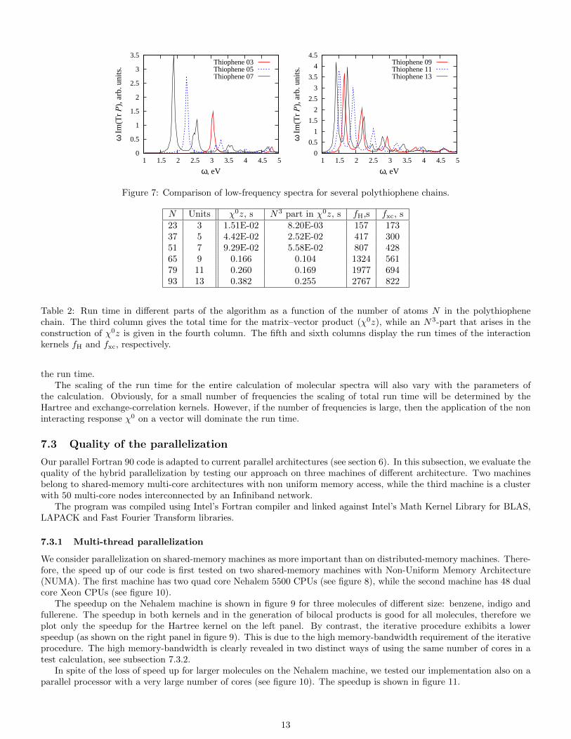
Sulfur containing molecules are widely use in organic electronics [32, 36, 37]. In this work, we study pure polythiophenechains of 3 to 13 repeating units. The geometry of the longest polythiophene we considered is shown in figure 6. Ourcalculations suggest (ignoring the excitonic character of these molecules) that the HOMO–LUMO energy differencedecreases, while the absorption increases, with chain length. The calculated absorption spectra are collected in figure 7.

We now use the calculations on polythiophene spectra in order to study the run time scaling with the number of atomsof different parts of our algorithm. Their scaling behavior will be described in terms of approximate scaling exponents.The run times for a few chains are collected in table 2 for a machine of four CPU AMD Dual-Core Opteron @ 2.6GHz;8MB cache; 32GB DDR2 RAM, and running sequentially.

The application of the non interacting response to a vector consists of N2- and N3-parts (see subsection 4.2). Thetotal time for the product χ0 z is collected in the third column of table 2, while the run time of the N3-part is collectedin the fourth column. Using the run times, one can compute exponents x and x3 for their corresponding scaling laws Nx

and Nx3 . The exponents x and x3 vary in the range of x = 2.31 . . . 2.36 and x3 = 2.49 . . . 2.53, respectively. The run timeof the Hartree kernel (fifth column) shows a scaling exponent in the range xH = 2.05 . . . 2.06, while the run time in theexchange–correlation kernel (sixth column) scales almost linearly xxc = 1.04 . . . 1.12. Therefore, the measured exponentsare close to the predicted exponents x = 3, x3 = 3, xH = 2, and xxc = 1.

The calculation of the Hartree kernel fH via multipoles, as explained in subsection 5.1 improves the run time in thecase of large molecules, but could not improve the run time scaling of the Coulomb interaction. In fact, the Hartree kernelfH is a non-local quantity and the rotations involved in the bilocal dominant products contribute a substantial part to

12

0

0.5

1

1.5

2

2.5

3

3.5

1 1.5 2 2.5 3 3.5 4 4.5 5

ω I

m(T

r P

), a

rb. u

nits

.

ω, eV

Thiophene 03Thiophene 05Thiophene 07

0

0.5

1

1.5

2

2.5

3

3.5

4

4.5

1 1.5 2 2.5 3 3.5 4 4.5 5

ω I

m(T

r P

), a

rb. u

nits

.

ω, eV

Thiophene 09Thiophene 11Thiophene 13

Figure 7: Comparison of low-frequency spectra for several polythiophene chains.

N Units χ0z, s N3 part in χ0z, s fH,s fxc, s23 3 1.51E-02 8.20E-03 157 17337 5 4.42E-02 2.52E-02 417 30051 7 9.29E-02 5.58E-02 807 42865 9 0.166 0.104 1324 56179 11 0.260 0.169 1977 69493 13 0.382 0.255 2767 822

Table 2: Run time in different parts of the algorithm as a function of the number of atoms N in the polythiophenechain. The third column gives the total time for the matrix–vector product (χ0z), while an N3-part that arises in theconstruction of χ0z is given in the fourth column. The fifth and sixth columns display the run times of the interactionkernels fH and fxc, respectively.

the run time.The scaling of the run time for the entire calculation of molecular spectra will also vary with the parameters of

the calculation. Obviously, for a small number of frequencies the scaling of total run time will be determined by theHartree and exchange-correlation kernels. However, if the number of frequencies is large, then the application of the noninteracting response χ0 on a vector will dominate the run time.

7.3 Quality of the parallelization

Our parallel Fortran 90 code is adapted to current parallel architectures (see section 6). In this subsection, we evaluate thequality of the hybrid parallelization by testing our approach on three machines of different architecture. Two machinesbelong to shared-memory multi-core architectures with non uniform memory access, while the third machine is a clusterwith 50 multi-core nodes interconnected by an Infiniband network.

The program was compiled using Intel’s Fortran compiler and linked against Intel’s Math Kernel Library for BLAS,LAPACK and Fast Fourier Transform libraries.

7.3.1 Multi-thread parallelization

We consider parallelization on shared-memory machines as more important than on distributed-memory machines. There-fore, the speed up of our code is first tested on two shared-memory machines with Non-Uniform Memory Architecture(NUMA). The first machine has two quad core Nehalem 5500 CPUs (see figure 8), while the second machine has 48 dualcore Xeon CPUs (see figure 10).

The speedup on the Nehalem machine is shown in figure 9 for three molecules of different size: benzene, indigo andfullerene. The speedup in both kernels and in the generation of bilocal products is good for all molecules, therefore weplot only the speedup for the Hartree kernel on the left panel. By contrast, the iterative procedure exhibits a lowerspeedup (as shown on the right panel in figure 9). This is due to the high memory-bandwidth requirement of the iterativeprocedure. The high memory-bandwidth is clearly revealed in two distinct ways of using the same number of cores in atest calculation, see subsection 7.3.2.

In spite of the loss of speed up for larger molecules on the Nehalem machine, we tested our implementation also on aparallel processor with a very large number of cores (see figure 10). The speedup is shown in figure 11.

13

Co

re 0

L2

25

6K

B

L1

32

KB

Co

re 1

L2

25

6K

B

L1

32

KB

Co

re 2

L2

25

6K

B

L1

32

KB

Co

re 3

L2

25

6K

B

L1

32

KB

Co

re 4

L2

25

6K

B

L1

32

KB

Co

re 5

L2

25

6K

B

L1

32

KB

Co

re 6

L2

25

6K

B

L1

32

KB

Co

re 7

L2

25

6K

B

L1

32

KB

RAM 24 GB RAM 24 GB

Cache L3 8MBCache L3 8MB

Figure 8: Memory/cache/core structure of Nehalem Intel Xeon X5550 machine. Two quad core nodes have a fast accessto one of the memory banks, while the inter node communication is slower.

0

1

2

3

4

5

6

7

8

1 2 3 4 5 6 7 8

Spee

dup

fact

or

Number of threads

Hartree kernel

BenzeneIndigoFullerene C60

0

1

2

3

4

5

6

7

8

1 2 3 4 5 6 7 8Sp

eedu

p fa

ctor

Number of threads

Iterative procedure

BenzeneIndigoFullerene C60

Figure 9: The left panel shows the speedup factor in the Hartree kernel for molecules of different size. The speedup in theexchange-correlation kernel and in the generation of dominant products is similar to the left panel. The right panel showsthe speedup factor in the iterative procedure. We observe that the speed up decreases with the size of the molecule.

Our results show a satisfactory speedup in both interaction kernels, while the iterative procedure again shows a poorerperformance due its high memory bandwidth requirements, which cannot be satisfied in this NUMA architecture.

7.3.2 Hybrid MPI-thread parallelization

Prior to large scale computations with many Nehalem (see figure 8) nodes, we performed test runs on one node to find anoptimal OpenMP/MPI splitting. Four calculations were done on the Nehalem machine using all 8 cores of the machine,but differing in the OpenMP/MPI splitting. The results are collected in the table 3. We observed a small workloadunbalance of 8% in case of the Hartree kernel and an even smaller unbalance of 5% in the case of the exchange–correlationkernel. The iterative procedure with the “round robin distribution” of frequencies over the nodes shows a even lowerworkload unbalance of 2%. The best run time is achieved in a 2/4 hybrid parallelization i.e. running 2 processes with 4cores each. This optimal configuration reflects the structure of the machine, where each thread shares the same L3 cache.The node has two processors of four cores each and a relatively slower memory access between the processors. This weakinter node communication results in an appreciable penalty in an OpenMP-only run (1/8 configuration), because theiterative procedure reads a rather large amount of data (V abµ XE

b ) twice during the application of the response functionχ0 (see subsection 4.2).

L2(3MB) L2(3MB) L2(3MB)

L1(3

2K

B) C

OR

E 0

0

L1(3

2K

B) C

OR

E 0

1

L1(3

2K

B) C

OR

E 0

2

L1(3

2K

B) C

OR

E 0

3

L1(3

2K

B) C

OR

E 0

4

L1(3

2K

B) C

OR

E 0

5

L2(3MB) L2(3MB) L2(3MB)

...

L3(16MB) Sock 03

L1(3

2K

B) C

OR

E 1

8

L1(3

2K

B) C

OR

E 2

3

L1(3

2K

B) C

OR

E 2

2

L1(3

2K

B) C

OR

E 2

1

L1(3

2K

B) C

OR

E 2

0

L1(3

2K

B) C

OR

E 1

9

L3(16MB) Sock 00

RAM(48GB) NODES 00, 01, 02, 04

Figure 10: Memory/cache/core structure of Xeon-96 machine. 48 dual core Xeon CPUs are connected to four memorybanks. Although every core can address the whole memory space, the inter node communication is slower.

14

0

10

20

30

40

50

60

70

80

90

10 20 30 40 50 60 70 80 90

Spee

dup

fact

or

Number of threads

Indigo blue

Hartree kernelExchange-correlation kernelIterative procedure

0

10

20

30

40

50

60

70

80

90

10 20 30 40 50 60 70 80 90

Spee

dup

fact

or

Number of threads

Fullerene C60

Hartree kernelExchange-correlation kernelIterative procedure

Figure 11: Speedup on a heavily parallel Xeon-96 machine. The results are satisfactory for the interaction kernels, whilethe memory-bandwidth requirements of the iterative procedure hamper the parallel performance in the case of the largerfullerene C60 molecule.

Proc / Thr Domi. prod. fH fxc Iterative proc. Total1/8 7.3 271 142 145 5712/4 6.9 (6.9) 273 (267) 142 (141) 109 (108) 5384/2 6.8 (6.8) 274 (264) 142 (141) 122 (112) 5448/1 6.8 (6.8) 274 (257) 143 (140) 134 (120) 570

Table 3: Run time and speedup factors in a hybrid MPI/OpenMP parallelization for fullerene C60. In the brackets, thesmallest run time between the nodes is stated in order to estimate the MPI work load disbalance.

The high memory-bandwidth requirement is clearly revealed in two distinct ways of using the same number of cores (8cores), either using all cores on one node or distributing them over two nodes. In the latter case, the memory-bandwidthis higher and the iterative procedure runs considerably faster (92 seconds versus 137 seconds in the case of fullerene C60).

We used the above optimal 2/4 hybrid configuration in a massively parallel calculation on the chlorophyll-a molecule.The speedup due to hybrid OpenMP–MPI parallelization is shown in figure 12. In this computation, we used up to50 nodes of recent generation Nehalem machines. According to the previous experiment on fullerene C60, we started 2processes per node, each process running with four threads. The two processes were placed on sockets. One can see thatthe iterative procedure shows the best speedup among other parts of the code, while total run time is governed mainlyby the calculation of the exchange-correlation kernel. The absolute run times (including communication time) in the firstcalculation with one node (2 processes) were: total 4003 seconds, for the exchange-correlation kernel 1147 seconds, forthe Hartree kernel 1247 seconds, for the iterative procedure 1574 seconds, and for the bilocal vertex 11.8 seconds. Thespeedup in the bilocal vertex reaches a maximum at 10 nodes because of increasing communication time.

0 5

10 15 20 25 30 35 40 45 50

5 10 15 20 25 30 35 40 45 50

Spee

dup

fact

or

Number of nodes

Chlorophyll-a

Total runtimeExchange-correlation kernelHartree kernelIterative procedureBilocal vertex

Figure 12: Speedup due to hybrid OpenMP/MPI parallelization for chlorophyll-a. The job was run on up to 50 nodeswith 2 processes per node. The code shows a linear speedup on up to 15 nodes (30 processes, 120 cores). Further increaseof the number of nodes results in a steady acceleration of the whole program.

The starting geometry of the molecule was taken from Sundholm’s supplementary data [38]. The geometry was furtherrelaxed in the SIESTA package [34] using Broyden’s algorithm until the remaining force was less than 0.04 Ry/A. Therelaxed geometry is shown in figure 13. In order to achieve this (default) criterion, we had to use a finer internal mesh

15

with a MeshCutoff of 185 Ry. The default DZP basis was used, but to achieve convergence, we used orbitals that are moreextended in space than SIESTA’s default orbitals. The spatial extension is governed by the parameter PAO.EnergyShiftthat was set to 0.002 Ry in the present calculation. The spectrum of the chlorophyll-a molecule is seen in figure 14.Like in the case of fullerene C60, there is excellent agreements between theoretical results that however differ from theexperimental data [39]. The low frequency spectrum consists of two bands at 635 nm and 450 nm. Both bands are dueto transitions in the porphyrin. According to our calculation, the first A band consist of 2 transitions between HOMO–LUMO and HOMO-1–LUMO, while the second (so called Soret) band consist of 6 transitions to LUMO and LUMO+1states.

Figure 13: The relaxed geometry of chlorophyll-a molecule obtained with the SIESTA package using a DZP basis set.

0

0.2

0.4

0.6

0.8

1

400 450 500 550 600 650 700

ω I

m(T

r P

), a

rb. u

nits

.

λ, nm

ExperimentalQuant. EspressoOur method 1

Figure 14: Low frequency absorption spectrum of chlorophyll-a.

7.4 Fullerene C60 versus PCBM

Fullerenes are often modified in order to tune their absorption spectra or their transport properties [32, 40, 41]. In thiswork, we compute the absorption spectra of [6,6]-phenyl C61 butyric acid methyl ester (PCBM) and compare with thespectrum of pure fullerene C60. We use the same parameters as in the case of C60 in subsection 7.1. A relaxed geometryof PCBM was obtained using the SIESTA package [34] and using its default convergence criterion (maximal force lessthan 0.04 eV/A). Figure 15 shows the relaxed geometry. The absorption spectrum of PCBM is shown in figures 16 and17.

Figure 16 shows a comparison of our calculation with recent experimental results [41]. We can see that our resultshave similar features as the experimental data: the maxima at 350 nm agree well with a broad experimental resonance at355 nm, and a substantial “background” at longer wavelength is present both in the calculated and in the experimentalspectrum. In this calculation, we set the damping constant ε = 0.08 Ry and compute the spectrum in the range whereexperimental data are available. However, in order to better understand the difference introduced by the functional group,we compute the spectra in a broader range of energies with a smaller value of the damping constant ε = 0.003 Ry. Theresult is shown in figure 17.

One can see on the left panel of figure 17 that PCBM absorbs much stronger in the visible range. This is a consequenceof symmetry breaking and indicates a modified HOMO–LUMO gap. On the right panel of the figure, one can recognize themain difference between pure and modified fullerene. The high spatial symmetry of pure fullerene leads to a degeneracy

16

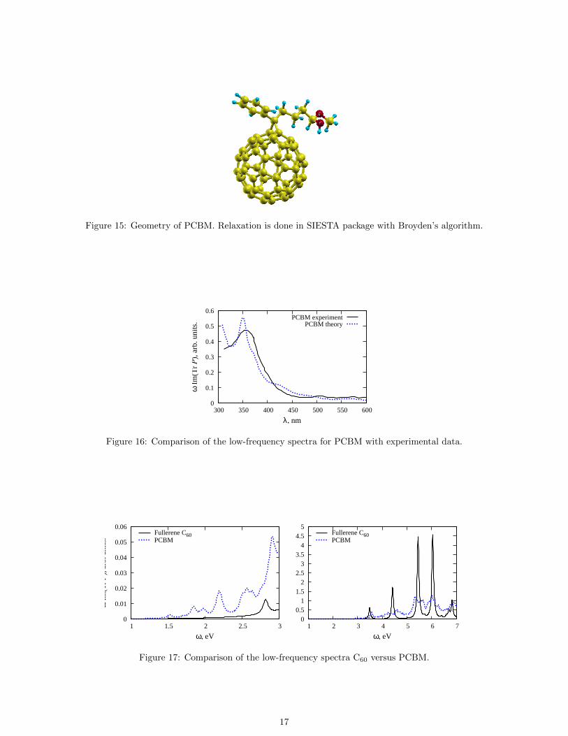
Figure 15: Geometry of PCBM. Relaxation is done in SIESTA package with Broyden’s algorithm.

0

0.1

0.2

0.3

0.4

0.5

0.6

300 350 400 450 500 550 600

ω I

m(T

r P

), a

rb. u

nits

.

λ, nm

PCBM experimentPCBM theory

Figure 16: Comparison of the low-frequency spectra for PCBM with experimental data.

0

0.01

0.02

0.03

0.04

0.05

0.06

1 1.5 2 2.5 3

ω I

m(T

r P

), a

rb. u

nits

.

ω, eV

Fullerene C60PCBM

0 0.5

1 1.5

2 2.5

3 3.5

4 4.5

5

1 2 3 4 5 6 7

ω, eV

Fullerene C60PCBM

Figure 17: Comparison of the low-frequency spectra C60 versus PCBM.

17

of the electronic transitions and several transition contribute to the same resonance. The symmetry is broken in the caseof PCBM, the degeneracy is lifted and the spectral weight is spread out.

8 Conclusion

In this paper, we have described a new iterative algorithm for computing molecular spectra. The method has two keyingredients. One is a previously constructed local basis in the space of products of atomic LCAO orbitals. The second isthe computation of the density response not in the entire space of products, but in an appropriate Krylov subspace.

The speed of our code is roughly comparable to TDDFT codes in commercially available software but the reader mustunderstand that we cannot give any details on this touchy issue.

The algorithm was parallelized and was shown to be suitable for treating molecules of more than hundred atoms onlarge current heterogeneous architectures using the OpenMP/MPI framework.

Our approach leaves plenty of room for further improvements both in the method and in the algorithm. For example,we did not consider reducing the dimension of the space in which the response function acts, but such a reduction isfeasible.

Also, we chose a uniform mesh on the frequency axis while a more economical, adaptive choice is possible. We areworking on an adaptive procedure to obtain good spectra with few frequency points and also to compute the position ofthe poles and strength of their residues. A reduction in the number of frequencies will allow to avoid the full calculationof the interaction kernels, replacing them by matrix-vector multiplications. There exist fast multipole methods [42] forcomputing fast matrix-vector products of the Hartree interaction.

Moreover, for large molecules, our embarrassingly parallel approach to compute spectra induces a memory-bandwidthbottleneck. To avoid it, one may parallelize the frequency loop using MPI and parallelize the matrix-vector operationsusing OpenMP.

More generally, because we do not use Casida’s equations, the methods developed here should be useful beyond theTDDFT approach, for instance in the context of Hedin’s GW approximation [43] where Casida’s approach is no longeravailable.

AcknowledgementWe are indebted to Gustavo Scuseria for calling our attention to the existence of iterative methods in TDDFT and

to Stan van Gisbergen for correspondence on the iterative method implemented in the Amsterdam Density Functionalpackage (ADF).

It is our special pleasure to thank James Talman (University of Western Ontario, Canada) for contributing two crucialcomputer codes to this project. We thank Luc Giraud (HiePACS, Toulouse) for discussions on the GMRES algorithmand our colleagues Aurelian Esnard and Abdou Guermouch (University of Bordeaux) for technical advice.

We acknowledge useful correspondence on the SIESTA code by Daniel Sanchez-Portal (DIPC, San Sebastian) andalso by Andrei Postnikov (Verlaine University, Metz). Advice by our colleagues of the ANR project CIS 2007 “NOSSI”especially Ross Brown and Isabelle Baraille (IPREM, Pau), is gratefully acknowledged. We also thank Uwe Huniak(Karlsruhe, Turbomole) for kindly supplying benchmarks of the TURBOMOLE package for comparison.

The results and benchmarks of this paper were obtained using the PlaFRIM experimental testbed of the INRIAPlaFRIM development project funded by LABRI, IMB, Conseil Regional d’Aquitaine, FeDER, Universite de Bordeauxand CNRS (see https://plafrim.bordeaux.inria.fr/).

The work was done with financial support from the ANR CIS 2007 “NOSSI” project.

References

[1] Time-Dependent Density Functional Theory, edited by M. A. L. Marques, C. A. Ullrich, F. Nogueira, A. Rubio,K. Burke, E. K. U. Gross (Springer, Berlin, 2008).

[2] A Primer in Density Functional Theory, edited by C. Fiolhais, F. Nogueira, M. A. L. Marques (Springer, Berlin,2003).

[3] E. Runge, E. K. U. Gross, Phys. Rev. Lett. 52, 997 (1984).

[4] M. A. L. Marques and E. K. U. Gross, Annu. Rev. Phys. Chem. 55, 427 (2004);

[5] M. Petersilka, U. J. Gossmann, and E. K. U. Gross, Phys. Rev. Lett., 76, 1212 (1996).

[6] M. E. Casida, in Recent Advances in Density Functional Theory, edited by D. P. Chong (World Scientific, Singapore,1995), p. 155.

18

[7] M. E. Casida, J. Mol. Struct.: THEOCHEM 914, 3 (2009).

[8] S. J. A. van Gisbergen, C. Fonseca Guerra, E. J. Baerends, J. Comput. Chem. 21, 1511 (2000).

[9] P.L. de Boeij, in Time-Dependent Density Functional Theory, edited by M. A. L. Marques, C. A. Ullrich, F. Nogueira,A. Rubio, K. Burke, E. K. U. Gross (Springer, Berlin, 2008).

[10] D. Rocca, R. Gebauer, Y. Saad, and S. Baroni, J. Chem. Phys. 128, 154105 (2008).

[11] D. Rocca, Time-dependent density functional perturbation theory. PhD Thesis (Scuola Internazionale Superiore diStudi Advanzati, 2004)

[12] D. Foerster, J. Chem. Phys. 128, 034108 (2008).

[13] D. Foerster, P. Koval, J. Chem. Phys. 131, 044103 (2009).

[14] P. Koval, D. Foerster, O. Coulaud, Phys. Status Solidi B accepted (2010).

[15] A. L. Fetter, J. D. Walecka, Quantum Theory of Many-Particle Systems (McGraw-Hill, New York, 1971).

[16] N. H. F. Beebe and J. Linderberg, Int. J. Quantum Chem. 7, 683 (1977).

[17] S. F. Boys, I. Shavitt., University of Wisconsin Naval Research Laboratory Report WIS-AF-13 (1959).

[18] C.-K. Skylaris, L. Gagliardi, N. C. Handy, A. G. Ioannou, S. Spencer, A. Willetts, J. Mol. Struct. THEOCHEM501–502, 229 (2000).

[19] E. J. Baerends, D. E. Ellis, P. Ros, Chem. Phys. 2, 41 (1973).

[20] G. Te Velde, F. M. Bickelhaupt, E. J. Baerends, C. Fonseca Guerra, S. J. A. van Gisbergen, J. G. Snijders, T. Ziegler,J. Comput. Chem. 22, 931 (2001).

[21] V. P. Vysotskiy and L. S. Cederbaum, arXiv:0912.1459v1 (2009).

[22] F. Aryasetiawan and O. Gunnarsson, Phys. Rev. B 49, 16214 (1994).

[23] U. Larrue, Etude de la densite spectrale d’une metrique associee a l’equation de Schrodinger pour l’hydrogene, un-published (Bordeaux, 2008). This study showed an asymptotically uniform density of eigenvalues, on a logarithmicscale, for the metric in the case of the hydrogen atom.

[24] Y. Saad, Iterative Methods for Sparse Linear Systems (Siam, Philadelphia 2003).

[25] V. Fraysse, Luc Giraud, Serge Gratton, and Julien Langou, Algorithm 842: A set of GMRES routines for real andcomplex arithmetics on high performance computers. ACM Trans. Math. Softw. 31, 228 (2005); http://doi.acm.org/10.1145/1067967.1067970.

[26] I. C. F. Ipsen and C. D. Meyer, The American Mathematical Monthly, 105, 889 (1998).

[27] R. Barrett, M. W. Berry, T. F. Chan, J. Demmel, J. Donato, J. Dongarra, V. Eijkhout, R. Pozo, Ch. Romine, andH. van der Vorst, Templates for the Solution of Linear Systems: Building Blocks for Iterative Methods (Society ofIndustrial and Applied Mathematics, 1993).

[28] J. D. Talman, Comput. Phys. Commun. 30, 93 (1983); Comput. Phys. Commun. 180, 332 (2009).

[29] I. S. Gradsteyn and I. M. Ryshik, Tables of Integrals, Series and Products (Academic Press, New York, 1980); formula6.578/4.

[30] V. I. Lebedev, Russ. Acad. Sci. Dokl. Math. 50, 283 (1995). http://www.ccl.net/cca/software/SOURCES/

FORTRAN/Lebedev-Laikov-Grids/

[31] http://openmp.org/wp/

[32] Ch. J. Brabec, N. S. Sariciftci, and J. C. Hummelen, Adv. Funct. Mater. 11, 15 (2001).

[33] R. Bauernschmit, R. Ahlrichs, F. H. Hennrich, and M. M. Kappes, J. Am. Chem. Soc. 120, 5052 (1998).

19

[34] P. Ordejon, E. Artacho and J. M. Soler, Phys. Rev. B 53, R10441 (1996); J. M. Soler, E. Artacho, J. D. Gale,A. Garcıa, J. Junquera, P. Ordejon, D. Sanchez-Portal, J. Phys. C 14, 2745 (2002). We used different branches ofSIESTA version 3 to perform calculations in this work.

[35] J. P. Perdew, A. Zunger, Phys. Rev. B 23, 5048–5079 (1981).

[36] F. Liang, J. Lu, J. Ding, R. Movileanu, and Ye Tao, Macromolecules 42, 6107 (2009).

[37] Y. Gao, Th. P. Martin, A. K. Thomas, and J. K. Grey, J. Phys. Chem. Lett. 1, 178 (2010).

[38] D. Sundholm, Chem. Phys. Lett. 302, 480 (1999) http://www.chem.helsinki.fi/~sundholm/qc/chlorophylla/

[39] H. Du, R. C. A. Fuh, J. Li, L. A. Corkan, and J. S. Lindsey, Photochem. Photobiol. 68, 141 (1998); http://omlc.ogi.edu/spectra/PhotochemCAD/html/index.html.

[40] A. C. Mayer, S. R. Scully, B. E. Hardin, M. W. Rowell, and M. D. McGehee, Materials today, 10, 28 (2007).

[41] P. Suresh, P. Balraju, G. D. Sharma, J. A. Mikroyannidis, and M. M. Stylianakis, ACS Appl. Mater. Interfaces, 11370 (2009).

[42] L. Greengard, V. Rokhlin, J. Comput. Phys. 73, 325 (1987); L. Greengard, Science 265, 909 (1994).

[43] L. Hedin, S. Lundqvist, Effects of Electron-Electron and Electron-Phonon Interactions on the One-Electron States ofSolids, in Solid State Physics, 23 (Academic Press, London, 1969).

20