HAL Id: tel-03253799https://tel.archives-ouvertes.fr/tel-03253799

Submitted on 8 Jun 2021

HAL is a multi-disciplinary open accessarchive for the deposit and dissemination of sci-entific research documents, whether they are pub-lished or not. The documents may come fromteaching and research institutions in France orabroad, or from public or private research centers.

L’archive ouverte pluridisciplinaire HAL, estdestinée au dépôt et à la diffusion de documentsscientifiques de niveau recherche, publiés ou non,émanant des établissements d’enseignement et derecherche français ou étrangers, des laboratoirespublics ou privés.

A one dimensional numerical coupling of the cerebralvasculature and the cerebrospinal fluid flow in the

cardio-spinal compartmentMarc Maher

To cite this version:Marc Maher. A one dimensional numerical coupling of the cerebral vasculature and the cerebrospinalfluid flow in the cardio-spinal compartment. Fluids mechanics [physics.class-ph]. Université PaulSabatier - Toulouse III, 2019. English. �NNT : 2019TOU30330�. �tel-03253799�

M. Jean-Pierre MARC-VERGNES, InvitéMme Muriel MESCAM, Invitée

Acknowledgments

J’aimerais tout d’abord remercier Patricia Cathalifaud, de m’avoir accompagné tout le longde mes travaux. Patricia, je te remercie de m’avoir aiguillé et conseillé dans cette recherche,dans laquelle j’ai pu apprendre "l’esprit" intuitive de la recherche et à me poser les questionsjustes. Je remercie également Mokhtar Zagzoule pour son encadrement et ses conseils avisés.Je remercie Olivier Balédent et Stéphanie Salmon d’avoir rapporté mon manuscrit de thèse etd’avoir partagé quelques pistes de réflexion concernant l’avenir de ces travaux ainsi que lesautres membres du jury, Jean-Pierre Marc Vergnes et Muriel Mescam.

Je souhaite remercier les membres du groupe ASI avec qui j’ai partagé un peu plus de troisans de quotidien dans des conditions de travail des plus agréables. Une mention spéciale àVéronique Roig, Patricia Hern, Nadine Mandement et Pierre Brancher pour leur bienveillanceainsi que leur soutien en fin de thèse.

Ce séjour m’as également permis de faire de belles rencontres qui ont pris part à monépanouissement dans ce travail. Et cela, je le dois entre autres à Loic, Karim, Aurélie, Johan,Guillaume, Tawfik, Marie et Elena que j’ai eu plaisir à côtoyer au cours de mon séjour à l’imft.

J’adresse mes remerciements les plus sincères aux figures inspirantes que j’ai côtoyéestout le long de ce travail : à commencer par Mady et Michel Geslin, merci à vous pournos discussions passionnantes entre neurosciences et humanisme, merci également pour votreaccompagnement invétéré et vos encouragements sans relâche. Je remercie également NicolasGeorges, ostéopathe D.O, d’avoir "synchronisé mon liquide céphalo-rachidien (LCR)" tout lelong de cette thèse et pour nos intéressants échanges autour du symbolisme émotionnel etspirituel du LCR.

J’adresse mes remerciements les plus tendres à Pauline Geslin, le pilier émotionnel, cellequi m’as accompagnée nuit et jour dans cet espace hors du temps qu’est la thèse. Pauline, jete remercie pour nos échanges mémorables et passionnants autour du LCR, d’avoir nourri etattisé ma curiosité à travers nos discussions. Merci pour tes sincères encouragements et tapleine présence. Il est sans doute énigmatique d’imaginer comment cette aventure se seraitdéroulée sans toi. Ce qui est certain, c’est que tu as participé à rendre ce voyage plein de sens.

Ensuite, du haut de ses 4 ans et né de la pluie de la deuxième année de thèse, je remerciemon fils Elliot, qui certainement sans le savoir a posé sa pierre à l’œuvre dans ce travail.

Enfin, c’est sans compter sur l’amour inconditionnel d’une mère qui m’as nourri et continuede me nourrir. A toi, Mona, je te dédicace ce travail, merci de m’avoir donné les moyens et lachance d’accomplir ces travaux et d’avoir sans aucun doute toujours cru en moi.

i

Résumé — Le liquide céphalo rachidien ou cérébro-spinal (LCS) s’écoule dans lesventricules cérébraux, les espaces sous arachnoidiens cérébraux et spinaux. Son écoulement estessentiel au fonctionnement normal du cerveau et sa perturbation est liée à des pathologiescérébrales. Un paramètre crucial directement lié à sa dynamique est la pression intracrâniennequi ne peut être mesurée que de manière invasive.

Dans cette thèse, en se basant sur l’hypothèse suivant laquelle le mouvement du LCSest principalement dûe à la pulsation artérielle cérébrale, nous modélisons numériquement lecouplage entre l’écoulement sanguin dans la vascularisation cérébrale (VC), depuis les voiesd’apports carotidiennes et vertébrales jusqu’aux veines jugulaires, et l’écoulement du LCSdans les espaces sous arachnoidiens cérébraux (ESAC) et spinaux (ESAS). La modélisation deces écoulements est basée sur les équations de Navier-Stokes unidimensionnelles (1D) dansune configuration de tubes coaxiaux et souples. Dans le compartiment cérébral, le réseau desESAC est coaxial à la VC tandis que dans le compartiment spinal, le réseau des ESAS estcoaxial à la moelle épinière.

Nos conditions aux limites sont les signaux de pression des artères carotidiennes, vertébraleset des veines jugulaires. Dans un premier temps, nous utilisons un signal de pression sinusoïdalet par la suite un signal de pression physiologique admettant plusieurs harmoniques. Notremodèle a permis de reproduire le caractère pulsatile du LCS et de mettre en évidence leséchanges de volume entre le compartiment crânien et spinal. Ainsi, lors d’une expansionvasculaire, nous avons pu reproduire la chasse du LCS crânien et son déplacement dans lecanal spinal, mettant en évidence son rôle de compensation volumique. Nous avons égalementpu retrouver des valeurs d’amplitude de débits de LCS cervical entre 0.5 et 3 mL/s en accordavec des données mesurés par IRM et de pression moyenne de CSF crânien entre 2 et 8 mmHg.La prise en compte de la compliance spinale a permis également de mettre en évidence desvaleurs de vitesse de propagtion du CSF spinal et d’atténuation de pression en accord avecdes mesures IRM.

Par la suite, nous avons procédé à une étude paramétrique dans laquelle nous nous sommesintéressés à l’influence de la variation du volume du LCS et de la compliance des espacessous arachnoidiens cérébraux et spinaux sur les pressions et débits dans la VC, les ESAC etles ESAS. Ces paramètres étant fortement liés aux pathologies crânio-spinales. Les résultatsmontrent une influence non négligeable de ces paramètres sur les maxima de débit, l’amplitudede pression et le stroke volume du LCS au niveau crânien de même que spinal. Un optimumde stroke volume du CSF spinal était atteint pour un volume global de LCS de 216 mL. Lemodèle a permis de mettre en évidence qu’une diminution de la compliance cranio-spinalepeut augmenter la pression intracrânienne et altérer l’écoulement du LCS. Enfin, nous avonsadapté notre modèle 1D à des données spécifiques issues de mesures IRM d’une population depersonnes saines ou avec des symptômes pathologiques et obtenu de bonnes corrélations entreles débits de LCS cervical calculés et mesurés.

Par la suite, cette étude permettra d’explorer le mécanisme d’autorégulation cérébrale sousla forme d’un problème de contrôle optimal en boucle fermée (dit feedback ou rétro-actif)

Mots clés : Pression intracrânienne, compliance cranio-spinale, modéli-sation 1d, couplage sang-LCS

Abstract — The cerebrospinal fluid (CSF) fills the ventricles, the cranial and spinalsubarachnoid spaces. CSF exhibits a pulsatile motion essential to normal brain function andits flow dynamics disturbance is linked to several CSF diseases. A relevant hemodynamicparameter, the intracranial pressure, which can be acquired only invasively is closely related toCSF flow dynamics. The main goal of this study is to build, based on the hypothesis that theCSF displacement is mainly driven by the cerebral arterial pulsation, a one-dimensional modelof the fluid mechanics coupling between the entire cerebral vasculature (CV) and the CSF.The CV is composed of 34 vessels depicting the arterial network, the microcirculation and thevenous network. It starts from the carotid and vertebral arteries to the jugular veins and issurrounded by the cranial subarachnoid spaces. This cranial vault is then coupled to a spinalvault which consists of the spinal cord enclosed by the spinal subarachnoid spaces. Blood andCSF are considered viscous. The blood vessels and the dura mater are assumed compliants.

The boundary conditions of the blood-CSF 1D model consist of an arterial pressure signalat the inlet of the carotid and vertebral arteries and a venous steady pressure at the jugularveins. First, a sinusoidal waveform of the arterial pressure signal is employed followed by aphysiological waveform signal. The study evaluates the effect of the dura mater elastance,the CSF volume and the lumbar cistern compliance on blood and CSF dynamics as theircontributions are closely related to CSF disorders. First, the model was able to reproduce theCSF flow pulsatility and fluids volume exchange between the cranial and spinal compartment.We found cervical CSF peak flow between 0.5 and 3 mL/s and cranial CSF pressure between 2and 8 mmHg which is in agreement with MRI studies. Moreover, due to the compliant spinalsubarachnoid spaces, pulse wave velocity and pulse pressure attenuation were find decreasingunder increasing spinal compliance.

A parametric analysis was conducted to quantify the effect of CSF volume and overallcranio-spinal compliance. Our results provide evidence of an optimal spinal CSF stroke volumefor a CSF volume of 216 mL. Moreover, cranial CSF pressure was found increasing underdecreasing the overall cranio spinal compliance. Finally, the model was confronted to PC-MRImeasurements and we found good agreement between computed and measured cervical CSFflow.

This work constitutes the object of future studies regarding the modeling of the cerebralautoregulation mechanism as a retroactive optimal process.

Keywords:Intracranial pressure, cranio-spinale compliance, 1d modelling,blood-csf coupling

iv

Contents

Table of Acronyms and Abbreviations xv

1 Introduction 1

1.1 Historical facts about CSF discovery . . . . . . . . . . . . . . . . . . . . . . . 2

1.2 Basic concepts of brain physiology: the relationship between the cerebrospinalfluid and the intracranial pressure . . . . . . . . . . . . . . . . . . . . . . . . 3

1.3 Physiopathology of the cerebrospinal fluid system . . . . . . . . . . . . . . . . 5

1.4 Motivation . . . . . . . . . . . . . . . . . . . . . . . . . . . . . . . . . . . . . 6

1.5 Methodolgy . . . . . . . . . . . . . . . . . . . . . . . . . . . . . . . . . . . . . 7

1.6 Work context . . . . . . . . . . . . . . . . . . . . . . . . . . . . . . . . . . . . 8

2 Anatomy and physiology of the central nervous system: a focus on thecerebrospinal fluid, the cerebral vasculature and the meninges 9

2.1 Introduction: an anatomical scope of the major components involved in this study 9

2.2 The cranial and spinal meninges: beyond their protective functions . . . . . . 10

2.3 The brain ventricular system . . . . . . . . . . . . . . . . . . . . . . . . . . . 12

2.4 Arterial supply and venous drainage of the CNS: a great deal of variability . 13

2.5 Cerebrospinal fluid motion and its coupling to the cerebral vasculature . . . . 15

3 The 1D craniospinal blood-CSF model 19

3.1 Introduction . . . . . . . . . . . . . . . . . . . . . . . . . . . . . . . . . . . . . 19

3.2 The cerebral vasculature : the 1D blood model from Zagzoule and Marc Vergnes 19

3.3 Subarachnoid spaces . . . . . . . . . . . . . . . . . . . . . . . . . . . . . . . . 21

3.4 Cranio-spinal compliance . . . . . . . . . . . . . . . . . . . . . . . . . . . . . 25

4 The 1D flow equations in a system of coaxial tubes 27

4.1 Introduction . . . . . . . . . . . . . . . . . . . . . . . . . . . . . . . . . . . . . 27

v

4.2 Mathematical Formulation . . . . . . . . . . . . . . . . . . . . . . . . . . . . . 27

4.3 Numerical scheme: the two steps Lax-Wendroff scheme . . . . . . . . . . . . . 33

4.4 Boundary conditions . . . . . . . . . . . . . . . . . . . . . . . . . . . . . . . . 35

4.5 Branching conditions . . . . . . . . . . . . . . . . . . . . . . . . . . . . . . . . 39

5 Blood-CSF coupling effect on the cerebral vasculature and CSF dynamics 45

5.1 Introduction . . . . . . . . . . . . . . . . . . . . . . . . . . . . . . . . . . . . . 45

5.2 An arterial sinusoidal waveform . . . . . . . . . . . . . . . . . . . . . . . . . . 46

5.3 Effect of varying the confinement and assessment of CSF viscosity . . . . . . 53

5.4 Effect of the cranio-spinal compliance . . . . . . . . . . . . . . . . . . . . . . 55

5.5 Effect of varying the cranial subarachnoid spaces compliance . . . . . . . . . 57

5.6 Effect of varying the spinal subarachnoid spaces compliance . . . . . . . . . . 58

5.7 An arterial physiological waveform . . . . . . . . . . . . . . . . . . . . . . . . 60

5.8 Conclusion . . . . . . . . . . . . . . . . . . . . . . . . . . . . . . . . . . . . . 61

6 Applications on patient specific Data 63

6.1 Introduction . . . . . . . . . . . . . . . . . . . . . . . . . . . . . . . . . . . . . 63

6.2 Data aquisition . . . . . . . . . . . . . . . . . . . . . . . . . . . . . . . . . . . 64

6.3 Patient specific 1D blood-CSF model . . . . . . . . . . . . . . . . . . . . . . . 64

6.4 CSF network parameters . . . . . . . . . . . . . . . . . . . . . . . . . . . . . . 65

6.5 Comparison between PC-MRI flow and 1D model flow . . . . . . . . . . . . . 65

6.6 Conclusion . . . . . . . . . . . . . . . . . . . . . . . . . . . . . . . . . . . . . 66

Conclusion 69

6.7 Conclusion . . . . . . . . . . . . . . . . . . . . . . . . . . . . . . . . . . . . . 69

6.8 Perspectives . . . . . . . . . . . . . . . . . . . . . . . . . . . . . . . . . . . . . 70

A Wall shear stresses in an annular flow 71

vi

B Branching conditions 75

B.1 A jonction of tubes . . . . . . . . . . . . . . . . . . . . . . . . . . . . . . . . . 81

B.2 A Bifurcation of tubes . . . . . . . . . . . . . . . . . . . . . . . . . . . . . . . 92

C A one dimensional model of the Cerebrospinal Fluid Flow in the spinalcanal: study of the fluid viscosity and the steady/unsteady flow effects 101

D CSF cervical flow computed from 1D model vs. MRI Data 121

Bibliography 128

vii

List of Figures

1.1 (a) Cerebral autoregulation mechanism. (b) The relationship between intracra-nial pressure and intracranial volume . . . . . . . . . . . . . . . . . . . . . . . 4

1.2 From outwards to inwards: the meninges, the central nervous system and theventricles . . . . . . . . . . . . . . . . . . . . . . . . . . . . . . . . . . . . . . 5

1.3 CSF disorders. (a) Hydrocephalus, (b) Chiari malformation type 1 . . . . . . 7

2.1 Anatomical terminology adapted from Neurosciecne 2nd edition [51] . . . 10

2.2 Cranial and spinal meninges adapted from Netter’s atlas of human anatomy7th edition[50] . . . . . . . . . . . . . . . . . . . . . . . . . . . . . . . . . . . . 11

2.3 The ventricular system . . . . . . . . . . . . . . . . . . . . . . . . . . . . . . 12

2.4 Arterial supply of the brain adapted from Netter’s atlas of human anatomy 7thedition[50] . . . . . . . . . . . . . . . . . . . . . . . . . . . . . . . . . . . . . . 14

2.5 Venous drainage of the brain adapted from Netter’s atlas of human anatomy7th edition[50] . . . . . . . . . . . . . . . . . . . . . . . . . . . . . . . . . . . . 15

2.6 Arterial supply and venous drainage of the spinal cord adapted from Netter’satlas of human anatomy 7th edition[50] . . . . . . . . . . . . . . . . . . . . . . 16

2.7 (a) An idealized representation of the interaction between blood and CSF.The left figure depicts CSF flowing towards the spinal cord during cerebralvasculature dilatation following by, in the right figure, CSF flowing towards thebrain skull during cerebral vasculature contraction. (b) A coaxial configurationof two compliant vessels . . . . . . . . . . . . . . . . . . . . . . . . . . . . . . 17

3.1 Morphological an rheological data used in Zagzoule et a. 1D model [73] . . . 20

3.2 The 1d model from Zagzoule and Marc Vergnes [73] . . . . . . . . . . . . . . 21

3.3 The 1d coupled blood-csf model. Red: blood vessels, blue: cranial subarachnoidspaces, orange: spinal subarachnoid spaces, green: CSF between the cranialand spinal vault, grey: the spinal cord. Dotted circles depict the branchinginterfaces between the cranial and the spinal vault . . . . . . . . . . . . . . . 22

3.4 Cranial subarachnoid space at full-scale for three values of cranial CSF confine-ment λcb . . . . . . . . . . . . . . . . . . . . . . . . . . . . . . . . . . . . . . . 24

ix

3.5 CSF volume (mL) for 0.1<λcb<0.85 . . . . . . . . . . . . . . . . . . . . . . . 25

3.6 Three elements R1R2Clw Windkessel model . . . . . . . . . . . . . . . . . . . 26

4.1 A one dimensional coaxial tubes where the inner tube represents a blood vesseland the outer tube a cranial sas where CSF flows . . . . . . . . . . . . . . . . 28

4.2 Wall shear stresses in a coaxial configuration . . . . . . . . . . . . . . . . . . 32

4.3 The Lax-Wendroff numerical scheme . . . . . . . . . . . . . . . . . . . . . . . 34

4.4 Boundary conditions of the 1D blood-CSF network . . . . . . . . . . . . . . . 36

4.5 Pressure signals imposed at the inlet of the blood vascualture. Two waveformsare considered : a sinusoidal and a physiological one . . . . . . . . . . . . . . 37

4.6 Three elements R1R2Clw Windkessel model . . . . . . . . . . . . . . . . . . . 38

5.1 Pressure and flow of the carotid artery, the jugular vein and the cervical CSFflow for a sinuoidal waveform . . . . . . . . . . . . . . . . . . . . . . . . . . . 47

5.2 Dimensionless Reynolds and Womersley number of the cerebral vasculature (cv)and the cranial subarachnoid spaces (csas) . . . . . . . . . . . . . . . . . . . . 49

5.3 From left to right : Pressure, flow and relative area temporal evolution ofarterioles (vessel 21) followed by the transverse sinus (vessel 31). c-m: coupledmodel, u-m: uncoupled model . . . . . . . . . . . . . . . . . . . . . . . . . . . 50

5.4 Blood peak flow and blood peak to peak pressure damping accross the coaxialcerebral vasculature . . . . . . . . . . . . . . . . . . . . . . . . . . . . . . . . 51

5.5 Phase lag to carotid artery flow. c-m: coupled-model, u-m: uncoupled-model 51

5.6 From left to right, pressure, flow and relative area temporal evolution of cranialsas coaxial to arterioles (vessel 21) and coaxial to transverse sinus (vessel 31) 52

5.7 (a) Mean pressure of the cerebral vasculature (cv). (b) Max., mean and min.of cranial CSF pressure . . . . . . . . . . . . . . . . . . . . . . . . . . . . . . 53

5.8 Blood and CSF fluids exchanges between the arterial, venous vasculature andthe cranial and spinal CSF. . . . . . . . . . . . . . . . . . . . . . . . . . . . . 54

5.9 Effect of CSF confinement or CSF volume on CSF peak flow, stroke volumeand mean pressure . . . . . . . . . . . . . . . . . . . . . . . . . . . . . . . . . 54

5.10 Evolution during a cycle of the conservation of momentum terms for threedifferent confinement λcb=0.3, 0.5 and 0.7 where Tq,t = ρdQ2/dt, Tp,z =(A2 −A1)dp/dz, Tq2,a,z = d(Aanr ∗Q2)/dz and Tf = 2π(R2τ2 −R1τ12). . . . 56

x

5.11 Effect of CSF viscosity on cranial CSF peak flow . . . . . . . . . . . . . . . . 56

5.12 Effect of intracranial compliance Cld on (working from top to bottom) venousflow, cranial CSF flow and spinal CSF flow . . . . . . . . . . . . . . . . . . . 58

5.13 Effect of spinal dura mater elasic modulus Eld on cranial, spinal CSF andvenous flow. . . . . . . . . . . . . . . . . . . . . . . . . . . . . . . . . . . . . . 59

5.14 Spinal volumetric compliance effect on spinal CSF pulse wave velocity (pwv) 59

5.15 Carotid, jugular and CSF flow for a physiological input waveform . . . . . . . 60

5.16 A physiological waveform: effect of CSF volume and cranio-spinal complianceon CSF flow. Ta-c: arterial to CSF cervical flow time delay, Ta-v: arterial tovenous flow time delay . . . . . . . . . . . . . . . . . . . . . . . . . . . . . . . 61

6.1 Cervical CSF flow computed from the current model and compared to measuredPC-MRI flow . . . . . . . . . . . . . . . . . . . . . . . . . . . . . . . . . . . . 67

xi

List of Tables

4.1 Mean value, a0 and Fourier coefficients ai, bi, i = 1, 2, ..., 6 of (4.32) whichcaptures the arterial pulsation . . . . . . . . . . . . . . . . . . . . . . . . . . . 38

5.1 Maximum, mean and minimum pressure-flow amplitudes of carotid artery 1,jugular vein 33 and cervical CSF for a sinusoidal arterial waveform . . . . . . 47

5.2 Maximum, mean and minimum pressure-flow amplitudes of carotid artery 1,jugular vein 33 and cervical CSF for a physiological arterial waveform . . . . 60

6.1 Mean blood and CSF flow . . . . . . . . . . . . . . . . . . . . . . . . . . . . . 64

6.2 Section of blood and CSF . . . . . . . . . . . . . . . . . . . . . . . . . . . . . 64

6.3 Computed nrmse, CSF volume, cranial and spinal sas compliance and pulsewave velocity in the spinal canal for 4 patients . . . . . . . . . . . . . . . . . 66

xiii

Table of Acronyms andAbbreviations

ICP Intracranial Pressure

CSF Cerebrospinal Fluid

sas Subarachnoid Space

cv Cerebral vasculature

CBF Cerebral Blood Flow

CPP Cerebral Perfusion Pressure

MAP Mean Arterial Pressure

ICC Intracranial Compliance

sc Spinal Cord

IV Intracranial Volume

PWV Pulse Wave Velocity

PC-MRI Phase Contrast - Magnetic Resonance Imaging

xv

Chapter 1

Introduction

1

1.1 Historical facts about CSF discovery

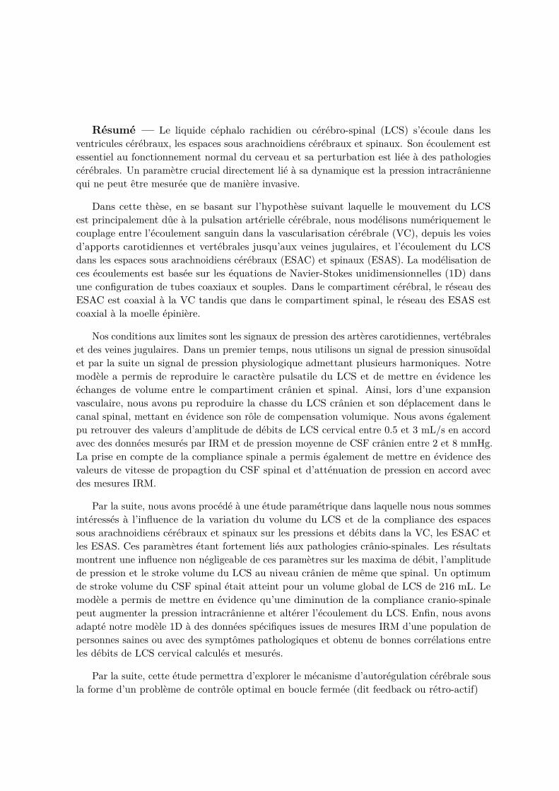
... is a clear fluid which fills larger spaces within and around the central nervous system(CNS) referred as subarachnoid spaces and brain ventricles. Since its first mentions, CSFhas been assigned countless origins and functions. Amongst them, Galen, a greek physicianand philosopher, considered CSF as the spirit of animal and described it as a vaporoushumor in the ventricles that provided energy to the entire body whereas Sutherland, one ofthe founding father of Ostheopathy has thought of the CSF as the breath of life. Thirtyphysicians and anatomists were at least involved in the CSF discovery. Among them,four greatest physicians should be considered as equal CSF’s discoverers. The Egyptianphysician Imhotep is the most likely to be the first one to mention intracranial CSF invivo in 3000 B.C. Later, in 1536, the Italian anatomist Nicolo Massa described CSF withincerebral ventricles based on postmortem autopsies. Then, two centuries later, the italianphysician Domenico Cotugno Niccolo was the first one to describe CSF around spinalcord through experimental postmortem research. And last but not least, three centurieslater, the French physician François Magendie was the first to discover method of CSFpressure measurement and was able to lay the scientific foundation for development of theCSF dynamic research [30]. Illustration below titled "CSF discovery: from hieroglyphicssymbols to MRI acquisition" depicts from left to right The Papyrus of Smith by Egyptianphysician and architect Imhotep who first acknowledges the intracranial fluid presence,François Magendie’s book title from 1842 and an MRI Sagital of neutral tube section inwhich CSF is red-colored. Until now, the CSF production, absorption and circulation isstill the topics of many debates amongst the clinical community.

The cerebrospinal fluid ...

2

1.2 Basic concepts of brain physiology: the relationship be-tween the cerebrospinal fluid and the intracranial pressure

The brain is a very complex organ which demands a continuous supply of oxygen. Although, itconstitutes 2% of the body mass, its oxygen consumption accounts for 20% for the total bodyoxygen consumption. Moreover, due to its lacking stores of glucose, it also needs a continuousdelivery of nutrients. Adequate oxygen and nutrients is supplied by the cerebral blood flow(CBF) via the cerebral vasculature (cv). The brain receives a CBF of 40 to 50mL/100 g oftissue per minute [61]. It is a vital need, as any reduction in CBF, known as cerebral ischaemia,occuring within seconds results in loss of consciousness and within 3-8 min in a permanentbrain damage.

Factors that affect the cerebral blood flow Blood flow through a vascular segmentmay be described as the ratio between the pressure difference (∆P ) accross that segment andits vascular resistance (R). According to the Hagen-Poiseuille equation, the blood flow (BF )through a vascular segment of length L, radius r and blood dynamic viscosity (µ), driven by apressure difference ∆P is given by,

BF = ∆PR

= π∆Pr4

8µL

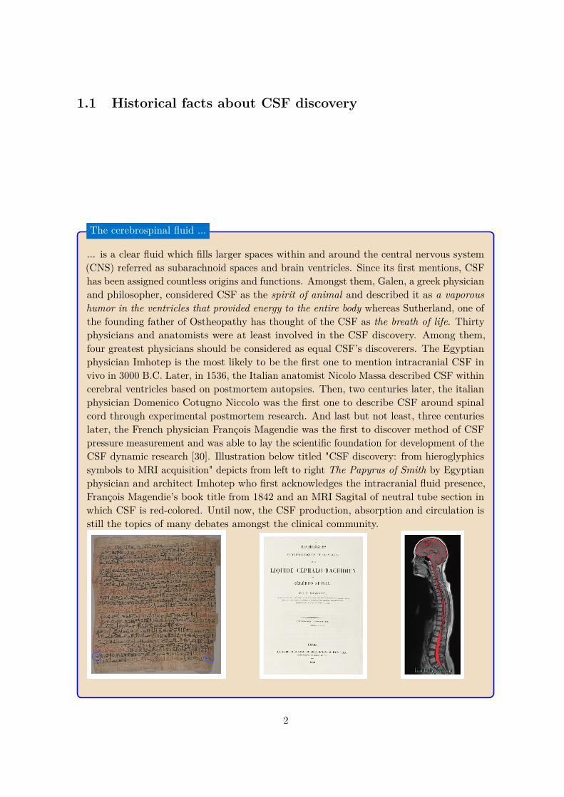
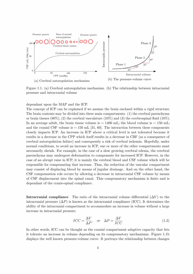
In the case of CBF, the driving pressure is known as the cerebral perfusion pressure (CPP),and the resistance is a total cerebrovascular resistance (CVR) which is related to the entirecerebral vasculature. CBF is therefore dependant upon the CPP, the CVR and the blooddynamic viscosity. For example, it will increases if the CPP increases and the CVR decreases.Under normal conditions, the CPP is variable and usually ranges between 70 and 90 mmHg .Variations in CPP may occur either under normal conditions, i.e during a change in postureor exercice or from pathological conditions such as traumatic brain injury or stroke. The CVRis affected by the small arteries, which can regulate their radius (r) through vasodilatationand vasoconstriction. Thus, when cerebral vasodilatation occurs, the increase in the radius ofthe vessels decreases the CVR and augments CBF. On the other hand, when vasoconstrictionoccurs, the CVR increases thus decreasing the CBF. This mechanism, diplayed figure 1.1a, isthe so-called cerebral autoregulation which is the brain ability to maintain CBF relativelyconstant despite changes in the CPP. The normal range of autoregulation occurs between 60and 150 mmHg of CPP, Beyond this plateau, CBF becomes pressure dependant.

Intracranial pressure The CPP is defined as the difference between the mean arterialpressure (MAP) and the intracranial pressure (ICP) which is the pressure in the cranial vault,

CPP = MAP − ICP (1.1)

Under normal conditions, the ICP is between 10 and 20 mmHg in adults, 3 and 7 mmHgin children and 1.5 and 6 mmHg in newborns. Following the latter equation, the CPP is

3

0 50 100 150CPP (mmHg)

CB

F(m

L/10

0g/m

in)

Cerebral autoregulation

100

50

0

Pressure passive Zone of normal autoregulation

Pressure passive

Cerebral blood volume

(a) Cerebral autoregulation mechanism

ΔPIntr

acra

nila

pre

ssur

e

Phase 1

Phase 2

Phase 3

Intracranial volume

ΔV

ΔP

ΔV

ΔP

ΔV

(b) The pressure-volume curve

Figure 1.1: (a) Cerebral autoregulation mechanism. (b) The relationship between intracranialpressure and intracranial volume

dependant upon the MAP and the ICP.The concept of ICP can be explained if we assume the brain enclosed within a rigid structure.The brain contents may be divided into three main compartments: (1) the cerebral parenchymaor brain tissues (80%), (2) the cerebral vasculature (10%) and (3) the cerebrospinal fluid (10%).In an average adult, the brain tissue volume is ∼ 1400 mL; the blood volume is ∼ 150 mL;and the cranial CSF volume is ∼ 150 mL [31, 60]. The interaction between these componentsclosely impacts ICP. An increase in ICP above a critical level is not tolerated because itresults in a decrease in the CPP which itself results in a decrease in CBF (as a consequence ofcerebral autoregulation failure) and consequently a risk of cerebral ischemia. Hopefully, undernormal conditions, to avoid an increase in ICP, one or more of the other compartments mustnecessarily shrink. For example, in the case of a slow growing cerebral edema, the cerebralparenchyma may undergoes deformation to compensate for increased ICP. However, in thecase of an abrupt raise in ICP, it is mainly the cerebral blood and CSF volume which will beresponsible for compensating that increase. Thus, the reduction of the vascular compartmentmay consist of displacing blood by means of jugular drainage. And on the other hand, theCSF compensation role occurs by allowing a decrease in intracranial CSF volume by meansof CSF displacement into the spinal canal. This compensatory mechanism is finite and isdependant of the cranio-spinal compliance.

Intracranial compliance The ratio of the intracranial volume differential (∆V ) to theintracranial pressure (∆P ) is known as the intracranial compliance (ICC). It determines theability of the intracranial compartment to accommodate an increase in volume without a largeincrease in intracranial pressure.

ICC = ∆V∆P , or ∆P = ∆V

ICC(1.2)

In other words, ICC can be thought as the cranial compartment adaptive capacity that letsit tolerate an increase in volume depending on its compensatory mechanisms. Figure 1.1bdisplays the well known pressure-volume curve. It portrays the relationship between changes

4

The Meninges

Spinal MeningesDura-mater Arachnoid Subarachnoid space Pia mater

Cranial MeningesDura-mater Arachnoid Subarachnoid space Pia mater

CNS

Brain

Spinal Cord

Ventricles

3

2

1

Figure 1.2: From outwards to inwards: the meninges, the central nervous system and theventricles

in ICP and intacranial volume and may be divided into three phases, (1) Phase 1: A highcompliance and low ICP. Despite the increase in volume, there is barely or a slight increasein ICP. CSF and cerebral blood volume buffering mechanisms are effective, (2) Phase 2 : Alower compliance and still a low ICP. But it starts to increase slowly as intracranial volumerises and finally, (3) Phase 3 : an inexisting compliance and high ICP. Buffering mechanismsare failling thus any small increase in intracranial volume results in a high increase in ICP.

1.3 Physiopathology of the cerebrospinal fluid system

During the previous section, we have demonstrated the crucial role and function of the CSFsystem acting as a buffering mechanism to ensure a steady ICP under normal conditions.However, in cases of abnormal CSF flow, the regulation of ICP is consequently disrupted.

In this section, we briefly present several prominent diseases that disrupt CSF dynamics.But first, we need to describe elementary anatomical aspects of the Central Nervous System(CNS).

Figure (1.2) displays the major components of the CNS. Working inwards from the skulllies the meninges 1 , a system of three connective tissue layers. These are the dura mater, thearachnoid and the pia mater. The interval between the arachnoid membrane and the pia materis called the subarachnoid space and is filled by CSF. The meninges covers the central nervoussystem (CNS) 2 , composed of the brain and the spinal cord, and their vasculature. CSF isbelieved to be mainly produced by ependymal cells, called the choroid plexus, which line theventricles 3 , a set of four connected cavities. The ventricles are connected to cranial andspinal subarachnoid spaces through CSF filled foramina (openings) and CSF filled cisterns.

5

Hydrocephalus Hydrocephalus is a pathological disorder resulting from an inappropriatevolume of CSF in the cerebral ventricles at an inappropriate pressure. Its symptom reflectsincreased ICP. Imaging hydrocephalus portrays enlargement of the cerebral ventricles withclinical evidence of inappropriately elevated pressure in the ventricles. Hydrocephalus resultsfrom either altered malabsorption of CSF at the arachnoid vili or direct obstruction by meansof aqueductal of Sylvius stenosis. Clinical treatment of the stenosis is through removal of theobstructing lesion.

Chiari malformation type I Chiari malformation type 1 results from the extension ofthe lower part of the cerebellum (called the cerebellar tonsils) below the level of the foramenmagnum into the cervical sas resulting in a alteration of CSF flow and pulsatility in the cranialcompartement. Clinical treatment of CM1 consist of removing small sections of the bone toensure enlargement of the cranio-cervical junction sas.

Syringomyelia Syringomyelia is a medical condition in which one or more fluid cavities(syrinxes) form within the spinal cord. The syrinxes often occur near locations of the spinalcord where spinal subarachnoid space is obstructed.

Although recent and ongoing progress in medical imaging is providing numerous data andnew insights about the dynamics interactions of the CNS and its pathological disorders, yetthe underlying physiological mechanisms of the interactions between CSF dynamics, ICP andarterial dynamics remains poorly understood. Computational model are therefore neededto provide additional predictions and interpretation of in vivo data acquired by means ofmedical imaging. Of special relevance, the strong coupling between arterial pulsations andCSF flow which is considered crucial in elucidating the pathophysiology of cerebrovascularand craniospinal diseases mentioned previously.

1.4 Motivation

There are numerous mathematical modelling of CSF flow in the cranium and the spinal vault.Moreover, most of these CFD models use rigid walls and finite domains such as a short segmentof the sas which requires boundary conditions that are adjusted to meet the desired velocities.However, there are few models accounting for closed models of the CNS, i.e the interactionbetween the cranial and the spinal compartment, and accounting for compliant walls. Todate and to our knowledge, there are a few models of a full CSF flow in the CNS. The firstwas developped by Lininger et al. [41] and consisted of multi-compartments model of thevascular system, the parenchyma and the CSF system. The model was able to predict CSFvelocities through the entire CNS as driven by arterial pulsations and simulates in a simplifiedmanner communicating hydrocephalus. However, authors have chosen to neglect unsteadyand convective inertia terms for convenience, thus ignoring the important and well recognizedrole played by waves reflection in vascular and CSF dynamics. This model was extended to asubject specific 3D model to quantify fluid interactions between cranial and spinal CSF with a

6

(a) Hydrocephalus disorder. (Left figure) A nor-mal brain. (Right figure) A hydrocephalic braindisplaying enlarged ventricles

Extension of cerebellum

Small sectionsof bone removed

Decompression

(b) Chiari malformation type 1

Figure 1.3: CSF disorders. (a) Hydrocephalus, (b) Chiari malformation type 1

particular attention given to microstructures embedded within the spinal canal such as nerveroots. However, this model did not account for the main CSF motor function, i.e the cerebralarterial pulsations.

One dimensional models of compliant vessels have shown the ability to describe the majorfeatures of biological flows. Moreover, several comparison against in vivo and in vitro datahave raised confidence in applying the 1-D formulation to capture blood and CSF flow inthe craniospinal environment. In addition, due to their reduced computational expensecompared to higher dimensional computational fluid dynamics, one dimensional models allowfor parametric analysis, where specific parameters in the model can be altered to understandtheir distinct contribution on pulse wave propagation.

1.5 Methodolgy

In the current study, we propose to build a global one dimensional model of the interactionsbetween compliant vessels of the cerebral vasculature and the CSF system. The cerebralvaculature was based upon the work of of Zagzoule and Marc Vergnes [73] and consistedof compliant arteries, arterioles, capillaries, veinules, veins, venous sinus and jugular veins.The CSF system comprises compliant cranial and spinal subarachnoid spaces. The modelwill be described and outcomes compared to in vivo results from Cine phase-contrast MRImeasurements. The objective is to accurately quantify the dynamic interactions between bloodflow, cranial and spinal CSF flow and therefore indirectly ICP. Moreover, the aim of this workis to provide an appropriate coupled 1D blood-CSF modeling of the craniospinal environmentfor patient- specific simulations to gain insights in estimating mechanical and medical relevantparameters such as intracranial pressure, intracranial CSF volume and intracranial compliance.The present work will be structured as follows, chapter 2 describes the physiology and anatomyof the central nervous sytem with a particular attention given to the cerebral vasculatureand the CSF system. It also introduces the mechanical interactions between blood and CSFflow. Chapter 3 presents the 1-D mathematical formulation of the governing flow equations of

7

blood and CSF in a system of coaxial compliant tubes. Chapter 3 introduce the architectureof the coupled blood-CSF models and describes the CSF system parametres which are theCSF volume and the cranial and spinal subarachnoid spaces compliance. Chapter 4 performsa parametric analysis in which the effect of the latter CSF system on blood and CSF pulsewave propagation are described. Finally, in chapter 5, medical imaging data are used andconfronted to outputs of the current model.

1.6 Work context

The study was conducted at l’Institut de Mécanique des Fluides de Toulouse (IMFT) in France.It is part of a project called ROMBA (Retro-active and Optimal Modelling of Blood flowAutoregulation), funded by a French state program called IDEX (Initiatives d’excellence).ROMBA project aims to simulate cerebral blood flow autoregulation described previously asthe ability of the brain to maintain constant blood flow despite changes in cerebral perfusionpressures. The objective is a simulator tool and a clinical protocol, using the autoregulationtime course pattern to interpret the clinical status of the craniospinal system and its agingprocess. ROMBA project involved researchers from four laboratories of Toulouse: the Institutde Mathématique de Toulouse (IMT), the Institut de Mécanique des Fluides de Toulouse(IMFT), the Centre de Recherche Cerveau et Cognition (CerCo), the Institut des Sciences duCerveau de Toulouse and a fifth partner being the Amiens Hospital-University.

8

Chapter 2

Anatomy and physiology of thecentral nervous system: a focus onthe cerebrospinal fluid, the cerebral

vasculature and the meninges

Sommaire2.1 Introduction: an anatomical scope of the major components involved

in this study . . . . . . . . . . . . . . . . . . . . . . . . . . . . . . . . . . 92.2 The cranial and spinal meninges: beyond their protective functions . 102.3 The brain ventricular system . . . . . . . . . . . . . . . . . . . . . . . . 122.4 Arterial supply and venous drainage of the CNS: a great deal of

variability . . . . . . . . . . . . . . . . . . . . . . . . . . . . . . . . . . . . 132.4.1 The brain and its need of uninterrupted blood oxygen . . . . . . . . . . . 132.4.2 The spinal cord . . . . . . . . . . . . . . . . . . . . . . . . . . . . . . . . . 14

2.5 Cerebrospinal fluid motion and its coupling to the cerebral vasculature 15

2.1 Introduction: an anatomical scope of the major compo-nents involved in this study

Modelling the dynamics coupling between the cerebral vasculature and the cerebrospinal fluidrequires rigorous anatomical description and understanding of the craniospinal environment.

This chapter is best treated under two main headings. Section one provides a description ofthe meninges and the ventricular system. Section two provides a description of the cerebral andspinal vasculature. And finally, section three discusses the hydrodynamic couplings betweenthe cerebral vasculature and the CSF.

Anatomy of the craniospinal environment Describing the CNS requires an elementaryunderstanding of standards used in anatomical terminology. Figure (2.1) depicts the relative

9

Figure 2.1: Anatomical terminology adapted from Neurosciecne 2nd edition [51]

directional terms and planes of reference employed to specify location in the CNS and moregenerally in the body. In subfigure (A), anterior and posterior refer to front and back of thehead. Superior, and inferior indicates above and below the head. Rostral and caudal refer todirection toward the head and tail. For example, a rostral CSF flow refers to a flow directiontoward the head. A caudal CSF flow refers to a flow direction towards the end of the spinalcord.

Subfigure (B) depicts the major planes of section used in cutting or imaging the brain.For a body standing upright, horizontal planes (also referred to as axial or transverse planes)are parallel to the ground. The sagittal plane is the section that divides the two hemispheres.The coronal or frontal plane refers to sections parallel to the plane of the face.

2.2 The cranial and spinal meninges: beyond their protectivefunctions

The meninges are present along the cranial and the spinal compartement. They are composedof three layers: the dura mater, the arachnoid mater, and the pia mater. These tissuessurround the brain and spinal cord and house the cerebrospinal fluid (CSF) located withinthe subarachnoid space (sas).

Figure (2.2) depicts a schematic view of the cranial meninges, a longitudinal view of thespinal cord (sc) and a section view of the sc portraying the spinal meninges.

The pia mater is the innermost layer of the meninges. It adheres to every contour of thebrain and the spinal cord. It is separated from the arachnoid by the CSF-filled subarachnoidspace. Furthermore, it is a highly vascular space containing blood vessels that supply theunderlying surface of the brain and the spinal cord.

10

Superior sagittal sinus

Arachnoid granulation

ArachnoidSubarachnoid space

Pia mater

Dura mater(inner layer)

Dura mater(outer layer)

Base of the skul

Conusmedullaris(terminationof spinal cord)

Subarachnoidspace

Caudaequina

Termination ofdural sac

Lumbar cistern

Falx cereberi

Tentorium cerebelli

Dura mater

Dura mater

Cervical nerves

Thoracic nerves

Lumbar nerves

Sacral and coccygeal nerves

A Schematic viewCranial meninges

B Longitudinal viewSpinal cord

C Section viewSpinal meninges

C

Figure 2.2: Cranial and spinal meninges adapted from Netter’s atlas of human anatomy 7thedition[50]

The dura mater is the outermost layer of the meninges. In the brain, it is composed of twolayers where the outer layer is adherent to the inner skull’s surface. The deeper layer, knownas the meningeal layer divides the brain into compartments. The most prominent of theseare the falx cerebri and the tenorium cerebelli. In some locations, the two layers separateto provides channels, the dural venous sinuses, for return flow of the venous blood. At theforamen magnum, the cranial dura mater becomes continuous with the spinal dura mater. Ithas a single layer separated from the wall of the vertebral canal by the epidural space whichcontains adipose tissue and blood vessels. At the tapered caudal end of the spinal cord ,theconus medullaris, the spinal roots extend caudally traversing a considerable distance throughthe subarachnoid space of the lumbar cistern forming the cauda equina.

11

Left lateral ventricle Left interventricular foramen (of Monroe)

3rd ventricle

4th ventricle

Foramen of Magendie

Foramen of Luschka

Arachnoid

Dura mater

Bridging veins

Chroid plexus of lateral ventricle

Superior sagittal sinus

Subarachnoid space

Arachnoid granulations

Chroid plexus of 3rd ventricle

Cerebral aqueduct(of Sylvius)

Foramen of Luschka

Chroid plexus of 4th ventricle

Dura mater

Arachnoid mater

Subarachnoid space

Foramen of Magendie

A

B

Cerebral aqueduct(of Sylvius)

Schematic view of the ventricles

A sagittal view of the brain

Figure 2.3: The ventricular system

2.3 The brain ventricular system

The ventricular system, figure (2.3), is a series of four interconnected ventricles and their con-necting foramina (opening). The largest of these ventricles are the lateral ventricles (one withineach of the cerebral hemispheres). These are connected to the third ventricle by two openingscalled the interventricular foramen (of Monro). Later, the third ventricle opens into the cerebralaqueduct (of Sylvius) which connects into the fourth ventricle. Finally, the fourth ventricleis later connected to subarachnoid cisterns and opens to cranial and spinal subarachnoid spaces.

The small arrows displayed in figure (2.3) B ) portrays CSF presence within the ventricular system, the cranial and spinal subarachnoid spaces. CSF is believed to be mainlysecreted through a plexus of cells called the Choroid Plexus (ChPs) embedded within theventricles [68, 63, 17], while the remaining is being produced by other CNS structures such asthe ependymal wall, cerebral parenchyma, and interstitial fluid (ISF) [34, 63, 44]. The ChPshave a relatively simple structure. It consists of a single layer of epithelial cells lying on abasement membrane. Beneath the epithelial basement membrane is a network of fenestratedcapillaries supplied from both the internal carotid arteries and the vertebral artery [17, 72, 65].

In the brain, the arachnoid granulations, one way valves, expands from the subarachnoidspace into the venous sinuses, especially the superior sagittal sinus, allowing CSF to drain intothe venous blood. CSF may also be absorbed through nerve pathways into the extracraniallymphatic vessels [63] and arachnoid villi located at the origins of the spinal nerves [35, 56].

12

2.4 Arterial supply and venous drainage of the CNS: a greatdeal of variability

2.4.1 The brain and its need of uninterrupted blood oxygen

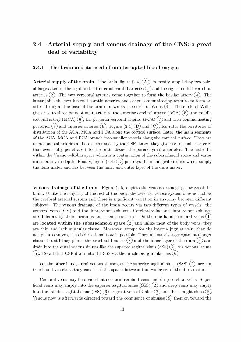
Arterial supply of the brain The brain, figure (2.4) A ), is mostly supplied by two pairsof large arteries, the right and left internal carotid arteries 1 and the right and left vertebralarteries 2 . The two vertebral arteries come together to form the basilar artery 3 . Thelatter joins the two internal carotid arteries and other communicating arteries to form anarterial ring at the base of the brain known as the circle of Willis 4 . The circle of Willisgives rise to three pairs of main arteries, the anterior cerebral artery (ACA) 5 , the middlecerebral artery (MCA) 6 , the posterior cerebral arteries (PCA) 7 and their communicatingposterior 8 and anterior arteries 9 . Figure (2.4) B and C illustrates the territories ofdistribution of the ACA, MCA and PCA along the cortical surface. Later, the main segmentsof the ACA, MCA and PCA branch into smaller vessels along the cortical surface. They arerefered as pial arteries and are surrounded by the CSF. Later, they give rise to smaller arteriesthat eventually penetrate into the brain tissue, the parenchymal arterioles. The latter liewithin the Virchow–Robin space which is a continuation of the subarachnoid space and variesconsiderably in depth. Finally, figure (2.4) D portrays the meningeal arteries which supplythe dura mater and lies between the inner and outer layer of the dura mater.

Venous drainage of the brain Figure (2.5) depicts the venous drainage pathways of thebrain. Unlike the majority of the rest of the body, the cerebral venous system does not followthe cerebral arterial system and there is significant variation in anatomy between differentsubjects. The venous drainage of the brain occurs via two different types of vessels: thecerebral veins (CV) and the dural venous sinuses. Cerebral veins and dural venous sinusesare different by their locations and their structures. On the one hand, cerebral veins 1are located within the subarachnoid space 2 and unlike most of the body veins, theyare thin and lack muscular tissue. Moreover, except for the interna jugular vein, they donot possess valves, thus bidirectional flow is possible. They ultimately aggregate into largerchannels until they pierce the arachnoid mater 3 and the inner layer of the dura 4 anddrain into the dural venous sinuses like the superior sagittal sinus (SSS) 2 , via venous lacuna5 . Recall that CSF drain into the SSS via the arachnoid granulations 6 .

On the other hand, dural venous sinuses, as the superior sagittal sinus (SSS) 2 , are nottrue blood vessels as they consist of the spaces between the two layers of the dura mater.

Cerebral veins may be divided into cortical cerebral veins and deep cerebral veins. Super-ficial veins may empty into the superior sagittal sinus (SSS) 2 and deep veins may emptyinto the inferior sagittal sinus (ISS) 6 or great vein of Galen 7 and the straight sinus 8 .Venous flow is afterwards directed toward the confluence of sinuses 9 then on toward the

13

Vertebral artery

Basilar artery

Posterior cerebralartery (PCA)

Posterior communicating artery

Internal carotidartery

Middle cerebralartery (MCA)

Anterior cerebralartery (ACA)

Anterior communicatingartery

Circle of Willis (dotted line)

Anterior cerebral artery

Middle cerebral arteryPosterior cerebral artery

Frontal view with hemispheres retracted

Lateral view Mid-sagittal view

A

Arachnoid granulations

Dura mater

Schema of meningeal arteries

B C

D

1

2

3

4

8

9

5

6

7

Middle meningealartery

Figure 2.4: Arterial supply of the brain adapted from Netter’s atlas of human anatomy 7thedition[50]

central circulation via the transverse sinus 10 , sigmoid sinus 11 , and ultimately empties intothe jugular veins. Along the jugular vein, there are several routes that allow complementaryvenous drainage in the brain in particular in the upright position.

2.4.2 The spinal cord

The spinal cord, (2.6), is mostly supplied by the anterior (ASA) and the paired posterior spinalarteries (PSA) which derives from the vertebral artery. Radicular arteries, such as the arteryof Adamkiewicz, deriving from the aorta, anastomose with ASA and PSA and reinforce the

14

A Sagittal view of the brain B Coronal view section of the brain

Arachnoid granulation

Arachnoid Subarachnoidspace

Pia mater

Dura mater(inner layer)

Dura mater(outer layer)

Venous lacuna

Falx cerebri

Superior sagittal sinus (SSS) 2

1

2

2

4

3

6

7

9

8

10

11

Superior sagittal sinus (SSS)

Sigmoid sinus

Straight sinus

Great cerebral vein (of Galen)

Transverse sinus

Confluence of sinuses

Inferior sagittal sinus (ISS)

B

Cerebral veins

Figure 2.5: Venous drainage of the brain adapted from Netter’s atlas of human anatomy 7thedition[50]

blood supply to the spinal cord. Later, the ASA and PSA penetrate through the subarachnoidspace giving rise to pial arterial plexus.Venous drainage largely follows arterial supply. An internal venoux plexus, located within theepidural space and the subarachnoid space drain into the anterior, posterior and radicularveins.

2.5 Cerebrospinal fluid motion and its coupling to the cerebralvasculature

In adults, mean CSF volume is estimated to be 150 mL with a distribution of 25 ml withinthe ventricles and 125 ml within the subarachnoid spaces. CSF forms at a rate of 500–600mL/day. Therefore, the CSF is replaced three to four times per day. [11, 17].CSF pulsates through the ventricular system. Magnetic resonance imaging (MRI) studieshave confirmed that the cardiac cycle imposes its pulsatile pattern onto the CSF dynamics[24, 70]. CSF also flows from the cranial to the spinal SAS in systole, with flow reversal fromthe spinal SAS into the cranium in diastole [28]. Besides cardiac driven pulsations, respirationinfluence on the CSF oscillations has been described in many radiological studies. It producesa modulation of the intracranial pressure resulting in a smaller additional oscillation of theCSF [37, 21].

Freund et al. 2001 [26] suggests, using MRI that the total cerebral blood volume inflatesand deflates in each cardiac cycle by approximately 1–2 mL, the same volumetric amount asthere is CSF exchange between the cranial and spinal SAS. In addition to CSF pulsations withno net flux, there is evidence of a small volumetric bulk component due to CSF production

15

Posterior cerebral artery

Basilar artery

Anterior spinal artery

Vertebral artery

Posterior spinal artery

Posterior spinal artery

Posterior spinal vein

Pia mater

Subarachnoid space

Dura mater

Internal venouxplexus

Anterior spinalvein

Pial arterialplexus

Pia venousplexus

Anterior spinal artery

Artery of Adamkiewicz(major anterior radicular artery)

Figure 2.6: Arterial supply and venous drainage of the spinal cord adapted from Netter’s atlasof human anatomy 7th edition[50]

and absorption.

So long, pulsatile CSF oscillations are believed to be driven by systolic vascular dilatationfollowed by diastolic contraction. From a mechanical point of view, this motion may beexplained based on a concept known as the Monro-Kellie dogma [48]. Because the skull isa rigid box, the sum of the volumes occupied by the brain, the vasculature, the meninges,the ventricular system and the CSF must remain constant. The spinal cord has the samecomponents but less rigid constraints on its total volume. Therefore, when the volume of oneof the components increases, the volume of another must decrease to compensate increase inICP. Thus, during a normal cardiac cycle, volume variation of the cerebral vasculature triggersCSF displacement.

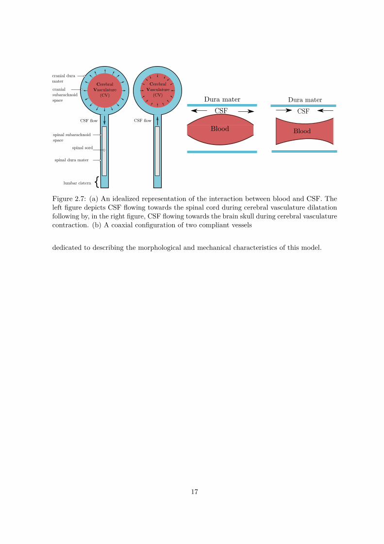
Figure (2.7) portrays the overall concept of the Monro-Kellie doctrine employed in thisstudy. The cranial compartment depicts the cerebral vasculature, the cranial subarachnoidspace and the cranial dura mater and is coupled to the spinal compartment composed of thespinal dura mater, the spinal cord and the lumbar cistern. Thus, in this work, the Monro-Kelliedogma is reduced in the brain compartment to two components being the cerebral vasculatureand the cranial subarachnoid space. Volumetric variations of the cerebral parenchym is beingneglected. Based on this concept, a simplified one-dimensional model was built involving thefollowing components of the CNS: the cerebral vasculature, the cranial and spinal subarachnoidspaces and finally the spinal cord.

Moreover, the dynamic coupling between a blood vessel and a cranial subarachnoid spacehas been approached using a model of two compliant and coaxial tubes as illustrated in figure(2.7) where the interior tube represents a blood vessel and the exterior tube represents a cranialsubarachnoid-space enclosed by the dura mater. CSF flows in the annular space. By assuminga dura mater more rigid than the blood vessel, consequently as blood vessel expands, CSFflows out and as the blood vessel contracts, CSF flows in. Based on this coaxial configuration,we have expanded the one dimensional cerebral vasculature of Zagzoule and Marc Vergnes[73] and build upon it CSF flow in the cranial and spinal vault. The next chapter will be

16

CerebralVasculature

(CV)

spinal sord

cranial dura mater

spinal dura mater

lumbar cistern

spinal subarachnoidspace

cranial subarachnoid space

CerebralVasculature

(CV)

CerebralVasculature

(CV)

CSF flow CSF flow

CSF

Dura mater

Blood

CSFDura mater

Blood

Figure 2.7: (a) An idealized representation of the interaction between blood and CSF. Theleft figure depicts CSF flowing towards the spinal cord during cerebral vasculature dilatationfollowing by, in the right figure, CSF flowing towards the brain skull during cerebral vasculaturecontraction. (b) A coaxial configuration of two compliant vessels

dedicated to describing the morphological and mechanical characteristics of this model.

17

Chapter 3

The 1D craniospinal blood-CSFmodel

Sommaire3.1 Introduction . . . . . . . . . . . . . . . . . . . . . . . . . . . . . . . . . . 193.2 The cerebral vasculature : the 1D blood model from Zagzoule and

Marc Vergnes . . . . . . . . . . . . . . . . . . . . . . . . . . . . . . . . . . 193.3 Subarachnoid spaces . . . . . . . . . . . . . . . . . . . . . . . . . . . . . . 21

3.3.1 Cranial subarachnoid spaces . . . . . . . . . . . . . . . . . . . . . . . . . . 213.3.2 Spinal subarachnoid spaces . . . . . . . . . . . . . . . . . . . . . . . . . . 24

3.4 Cranio-spinal compliance . . . . . . . . . . . . . . . . . . . . . . . . . . . 253.4.1 Elastic modulus of the dura mater . . . . . . . . . . . . . . . . . . . . . . 253.4.2 The lumbar cistern compliance . . . . . . . . . . . . . . . . . . . . . . . . 25

3.1 Introduction

In chapter 2, we have highlighted the fact that CSF oscillations and motion between thecranial and the spinal compartment are mainly driven by dilatation and contraction of thecerebral vasculature. In this chapter, we present the one dimensional model of blood and CSFcouplings in the cranio-spinal vault.

First, we recall the one-dimensional model of Zagzoule and Marc Vergnes [73]. Then, wedescribe the geometric configuration used to model the cranial and spinal subarachnoid spaces.Finally, we investigate their mechanical properties.

3.2 The cerebral vasculature : the 1D blood model from Zag-zoule and Marc Vergnes

Figure (3.2) portrays the 1D cerebral vasculature model from Zagzoule and Marc Vergnes [73].It consists of a simplified morphological scheme portraying the major segments of the brain

19

Figure 3.1: Morphological an rheological data used in Zagzoule et a. 1D model [73]

arterial supply and venous drainage. Blood was assumed to be a Newtonian fluid with densityρb = 1.06 kg.m−2 and dynamic viscosity of µb = 0.0035 Pa.s.

It starts at the paired internal carotid arteries (1, 2) and the paired vertebral arteries (3,4) followed by the basilar artery 5 & 6, the circle of Willis (from 7 to 14), the cerebral arteries,the middle (17, 18) and posterior (15, 16) cerebral arteries. The two anterior cerebral arteriesare represented by a single vessel (19). The vessel, 6bis, is a peripheral resistance which mayrepresent either the vertebrobasilar vascular system of the brain stem and the cerebellumor a complementary drainage pathways to the jugular veins. The three following tubes areregrouped into equivalent tubes of the principal collaterals of the cerebral arteries (20), thepial network (21) and the intracerebral arteries (22). Tube 23 represent the microcirculation.It includes the terminal arterioles, the pre-capillaries, the capillaries and the venulas. Tubes 24and 25 depict respectively the intracerebral and pial veins. Vessels 26, 27, 29 and 31 portray agroup of veins draining into the major sinuses 28, 30 and 32. Finally, they ultimately draininto the jugular veins (33, 34). Model data, including cross-section, length, number of vesselsfor the equivalent tubes and elastance are shown in table (3.1). In the work of Zagzoule andMarc Vergnes [73], the lengths, cross-sections and the number of vessels were taken from thelitterature when they were available [32, 39, 1] . The blood volume of the carotid arteries,the vertebral arteries and the circle of Willis is 13.03 mL. For the arterial system after thecircle of Willis, it is set to 43.187 mL. The microcirculation volume is 19.36 mL and finallythe venous system volume is 96.04 mL.

Geometric assumptions and simplifications that were implemented to design this modelare discussed in [73].

20

33 34

32

1

3 4 2

5

1

66bis

10

11 12

13 1415

17 18

19

20 21 22

9

31 30

29

28

27

26252423

16

Arterial Network

Microcirculation

Venous Network

WillisCircle

7 8

Figure 3.2: The 1d model from Zagzoule and Marc Vergnes [73]

3.3 Subarachnoid spaces

Figure (3.3) displays the architecture of the coupled 1d blood-csf model. As describedpreviously, red vessels depicts the cerebral vasculature ranged from vessel 1 to 34. Blue vesselsdepict the coaxial cranial subarachnoid tubes, they are coaxial to blood vessels starting frombifurcations (11-9), (7-8) and (10-12) to the transverse sinus vessel 32. Therefore, the carotidarteries 1 and 2, the vertebral arteries 3 and 4 and the jugular veins 33 and 34 are not directlycoupled to the cranial subarachnoid spaces. Orange tubes depicts the spinal subarachnoidspaces and the lumbar cistern vessels enclosing in grey area the spinal cord tube. The inletof the spinal subarachnoid spaces is assumed to be the cervical C2-C3 CSF area. Finallygreen areas represent subarachnoid spaces tubes that link the cranial ones to the spinal ones.They will be referred in this work as the cranio-cervical junction tubes. Dashed black circlesdisplay the branching interfaces between the different vessels, they will be discussed in thenext chapter.

3.3.1 Cranial subarachnoid spaces

As explained previously, the dynamic coupling between a cerebral blood vessel and a cranialsubarachnoid space was approached using a coupled coaxial tubes modelling. The inner tubeaccounts for a blood vessel, whereas the outer tube portrays the cranial subarachnoid spaceconfined by the cranial dura mater.

21

33 34

32

1

3 4 2

5

1

66bis

10

11 12

13 1415

17 18

19

20 21 22

9

31 30

29

28

27

26252423

16

7 8

Spinal Cord

lumbar cistern

csj inlet csj outlet

C2-C3 area

Figure 3.3: The 1d coupled blood-csf model. Red: blood vessels, blue: cranial subarachnoidspaces, orange: spinal subarachnoid spaces, green: CSF between the cranial and spinal vault,grey: the spinal cord. Dotted circles depict the branching interfaces between the cranial andthe spinal vault

22

As mentioned previously, pulsatile CSF oscillations are believed to be driven by systolicvascular dilatation followed by diastolic contraction. In order to accurately model this coupling,some crucial questions have been raised in this study : which vascular vessels contribute themost to the pulsations of the cranial CSF flow and its displacement into the spinal canal ? Isit the arterial system by means of its strong pulsations ? What about the compliant venoussystem which blood volume is far greater than the arterial system ? Finally what about theparenchymal matter and the microcirculation system ?

Indeed, the main arteries running along the cortical surface, the pial arteries, are theclosest to the cranial subarachnoid spaces. Thus, from a ’spatial’ point a view, their pulsationsmay contribute the most to driving the CSF flow. Smaller penetrating arterioles or themicrocirculation bed, embedded within the cerebral tissue may also distend. Their systolicexpansion and thus their volumetric dilatation would need to be transmitted to the surroundingtissues and produce CSF motion [23, 24]. In a similar way, the bed capillary may contributeto CSF pulsations. In a first approach, we have chosen to enclose the entire global vasculaturesystem within the cranial CSF. For this configuration, the major brain blood supply vessels,i.e the carotid, the vertebral arteries and the jugular veins vessels were not enclosed by thecranial CSF as they are located outside of the cranial vault.

A second important question was raised regarding the dimensions of the cranial subarach-noid spaces. In vivo, they have been measured by ultrasound (US), computed tomography(CT) and magnetic resonance imaging (MRI) mainly in neonates and infants as it may bea marker for the development of several neuropsychatric diosorders. Their width have beenacquired between the cranium and the cerebral hemisphere, refered as the craniocorticaldistance and between the two hemispheres. Studies have shown variable upper limits for thecraniocortical distance width rangin from 3.3 to 5 mm in neonates [25, 47, 49] to 4 to 10 mmin infants and adults [57, 38, 40, 33].

In this study, the sections of the cranial subarachnoid spaces were defined as follows: Adimensionless parameter referred as CSF confinement and denoted λ, is defined as the ratiobetween the sections of a blood vessel and a cranial sas.

0.1 < λcb = AbiAci

< 0.85 for i=6,. . . , 32. (3.1)

where Abi and Aci are respectively the sections of a blood vessel of the cv and a tube of thecranial sas i.

For example, figure (3.4) illustrates at a full scale three values of cranial CSF confinement,λcb (0.1, 0.5 and 0.85), for a blood vessel, of 0.5 cm. As λcb increases from 0.1 towards 0.85,the annular CSF space and its volume, in blue, decreases.

The cranial CSF confinement was assigned a constant value along the cerebral vasculature.For example a cranial CSF confinement of λcb = 0.7 implies following equation (3.1) :

• For the posterior cerebral arteries (15, 16), a cranial subarachnoid vessel of 0.070.7 = 0.1

23

λcb = 0.1 λcb = 0.5 λcb = 0.85

Figure 3.4: Cranial subarachnoid space at full-scale for three values of cranial CSF confinementλcb

cm2 and therefore an annular CSF space area of 0.1− 0.07 = 0.03 cm2,

• For the middle cerebral arteries (17, 18), a cranial subarachnoid vessel of 0.120.7 = 0.17

cm2 and therefore an annular CSF space area of 0.17− 0.12 = 0.05cm2.

As the cranial CSF confinement varies between 0.1 and 0.85, cranial CSF volume variesbeteween 85 mL and 1400 mL.

3.3.2 Spinal subarachnoid spaces

In a similar manner, the spinal compartment was modeled as two coaxial tubes in which theinner tube represents the spinal cord enclosed by the spinal pia mater and the outer tuberepresents the spinal subarachnoid space (SSS) enclosed by the spinal dura mater. Since,we are mainly interested in the CSF fluid transport in the spinal sas, the spinal cord wasconsidered as well a CSF-fluid filled tube.

We used a geometric coaxial tube in which the spinal cord and the spinal sas were heldconstant along the spinal cord. Sections and length were partially based on the previouslypublished FE-FSI models of the spinal cavity [8, 7]. Spinal cord and SSS sections were takenrespectively equal to ASSS = 1.6 cm2 and ASSS = 0.78 cm2 yielding to a spinal CSF volumeof 68 mL. Moreover, the spinal subarachnoid space length was taken longer, ASSS = 70 cm,than the spinal cord, ASC = 50 cm to account for the lumbar cistern.

Figure (3.5) depicts the cranial and spinal CSF volume for λcb values ranging between 0.1(a cranial CSF volume of 1400 mL) and 0.85 (a cranial CSF volume of 95 mL). As statedpreviously, spinal CSF volume was assumed constant and equal to 68 mL.

24

Figure 3.5: CSF volume (mL) for 0.1<λcb<0.85

3.4 Cranio-spinal compliance

3.4.1 Elastic modulus of the dura mater

The mechanical compliance is the ability of a compartment to accomodate a change in volumefor a corresponding change in pressure. The overall cranio-spinal compliance is of specialinterest in understanding regulation of the intracranial pressure and is determined by addingthe cranial and spinal compartments compliance. It is expected from anatomic consideration,that both compliance contributes differently to the overall cranio-spinal compliance. From ananatomical point of view, the spinal vault would contribute largely as the spinal CSF is lessconfined by rigid structures than in the cranial vault. In vitro biomechanical charaterisationperformed by several authors has demonstrated a highly nonlinear behaviour with a longitudinaland transverse Young’s modulus from 1.4-105 MPa (104 - 8.105 mmHg) and 0.08-7 MPa (6.102

- 5.104 mmHg) respectively[27, 54, 62, 45, 14, 18].

In previous numerical models, the dura mater was considered as a linear elastic materialmodel. Bertram et al.[9] and Cirovic et al. [15] have chosen the elastic modulus of the duramater to approximate the spinal sas wave speed measured by MRI. It was set equal to 1.25MPa (9.103 mmHg). The spinal dura mater was also investigated by several authors [10, 46,52] and showed an elastic Young’s modulus varying from 1-2.3 MPa (7.5 103 - 1.7 104 mmHg).

In this work, the dura mater and the spinal pia mater were as well represented by alongitudinal Young’s modulus.

3.4.2 The lumbar cistern compliance

The lumbar segment was terminated by a 3 elements Windkessel model described in figure(3.6). It was assigned a volumetric compliance Clw , the proximal resitance R1 is introducedto absorb the incoming waves and reduce artificial wave reflections and The distal resistanceR2 was taken high to limit CSF outflow from the lumbar segment.

25

R1 R2

CPin PoutPc

Qin Qout

Qc

Figure 3.6: Three elements R1R2Clw Windkessel model

26

Chapter 4

The 1D flow equations in a systemof coaxial tubes

Sommaire4.1 Introduction . . . . . . . . . . . . . . . . . . . . . . . . . . . . . . . . . . 274.2 Mathematical Formulation . . . . . . . . . . . . . . . . . . . . . . . . . . 27

4.2.1 Main assumptions for the fluid flow and the wall motion . . . . . . . . . . 284.2.2 3D Navier Stokes equations for incompressible fluids . . . . . . . . . . . . 294.2.3 1D reduced Navier Stokes equations for a single or interior vessel . . . . . 304.2.4 1D reduced Navier-Stokes equations in a system of coaxial tubes . . . . . 31

4.3 Numerical scheme: the two steps Lax-Wendroff scheme . . . . . . . . 334.4 Boundary conditions . . . . . . . . . . . . . . . . . . . . . . . . . . . . . 354.5 Branching conditions . . . . . . . . . . . . . . . . . . . . . . . . . . . . . 39

4.1 Introduction

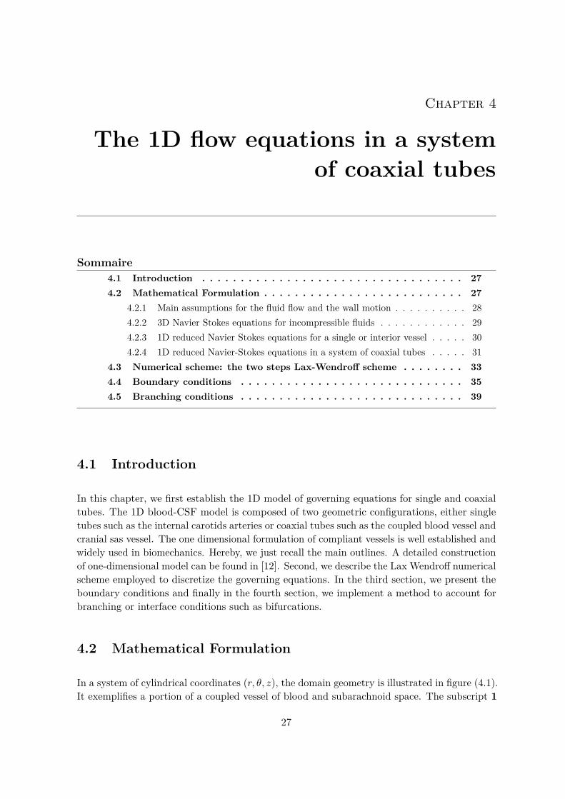
In this chapter, we first establish the 1D model of governing equations for single and coaxialtubes. The 1D blood-CSF model is composed of two geometric configurations, either singletubes such as the internal carotids arteries or coaxial tubes such as the coupled blood vessel andcranial sas vessel. The one dimensional formulation of compliant vessels is well established andwidely used in biomechanics. Hereby, we just recall the main outlines. A detailed constructionof one-dimensional model can be found in [12]. Second, we describe the Lax Wendroff numericalscheme employed to discretize the governing equations. In the third section, we present theboundary conditions and finally in the fourth section, we implement a method to account forbranching or interface conditions such as bifurcations.

4.2 Mathematical Formulation

In a system of cylindrical coordinates (r, θ, z), the domain geometry is illustrated in figure (4.1).It exemplifies a portion of a coupled vessel of blood and subarachnoid space. The subscript 1

27

A1

A2

Interior tube

Exterior tube U1

U2

z

R1rR2

Figure 4.1: A one dimensional coaxial tubes where the inner tube represents a blood vesseland the outer tube a cranial sas where CSF flows

denotes a single tube or an interior one whereas the subscript 2 denotes the exterior (annular)tube. The axis of the vessels is aligned along the coordinate z. R1 and R2 are respectively theinterior and exterior tube radius.

4.2.1 Main assumptions for the fluid flow and the wall motion

Blood was considered newtonian having respectively a dynamic viscosity µb = 0.035 Poise(g.cm−1.s−1) and density ρb = 1.06 g/mL. CSF was assumed close to water having dynamicviscosity µc = 10−2 Poise and ρb = 1 g/mL.

The one dimensional model for incompressible and newtonian fluid flow in a compliantvessel may be derived from the Navier Stokes equations, under the following simplifyinghypotheses.

When accounting for the fluid flow:

• Axial Symmetry, the dependance on θ is completely neglected. This implies that eachaxial section at a fixed z position remains circular at all times. We thus neglect anyeventual collapse of the tube. Therefore, the vessel radius, R1 (R2), is solely function ofz and t.

• Constant pressure in a cross section, the pressure is taken to be constant on each axialsection, so that it depends only on z and t.

• No body forces, such as gravity.

• Dominance of axial velocity, the velocity components orthogonal to z axis are negligiblecompared to the component along z. This consideration is sometimes called the LongWave-Length Approximation.

When accounting for the vessel structure:

• Radial displacement, the wall moves solely in the radial direction.

• Wall thickness, the effective wall thickness is relatively small and can be treated as amembrane.

28

• Small deformations gradients. We consider that the deformations gradients are relativelysmall, so that the structure behaves like a linear elastic solid.

4.2.2 3D Navier Stokes equations for incompressible fluids

Remarque 4.1Vectors are indicated using bold letters while their components will be denoted by the sameletter in normal typeface.

In Fluid mechanics, the fluid flow is governed by the following 3D incompressible Navier-Stokes equations,

∇.u = 0, (4.1)

ρ[∂u∂t

+ u.∇u] + ∇.[pI− τ ] = 0, (4.2)

The unknowns are the fluid velocity u = (ur, uθ, uz), the pressure p and the shear stresstensor τ . Due to the axisymmetric assumption, the shear stress tensor is defined as:

τ =

τrr 0 τrz0 τθθ 0τrz 0 τzz

where I is the identity matrix.

Using the assumptions established previsouly, the 3D incompressible Navier-Stokes equa-tions are reduced to the following system of equations ,

1r

∂(rur)∂r

+ ∂(uz)∂z

= 0, (4.3)

∂uz∂t

+ ur∂uz∂r

+ uz∂uz∂z

+ 1ρ

∂p

∂z= 1ρr

∂(rτrz)∂r

, (4.4)

p = p(z, t), (4.5)

where τrz is the wall shear stress defined as,

τrz = µ∂uz∂r

(4.6)

29

4.2.3 1D reduced Navier Stokes equations for a single or interior vessel

Remarque 4.2Subscript 1 is used for the inner tube whereas subscript 2 describes the outer tube.

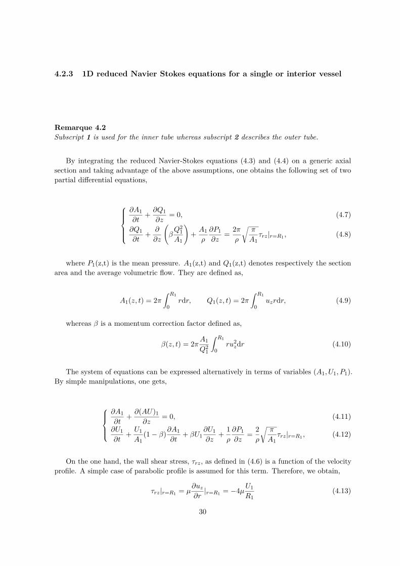
By integrating the reduced Navier-Stokes equations (4.3) and (4.4) on a generic axialsection and taking advantage of the above assumptions, one obtains the following set of twopartial differential equations,

∂A1∂t

+ ∂Q1∂z

= 0, (4.7)

∂Q1∂t

+ ∂

∂z

(βQ2

1A1

)+ A1

ρ

∂P1∂z

= 2πρ

√π

A1τrz|r=R1 , (4.8)

where P1(z,t) is the mean pressure. A1(z,t) and Q1(z,t) denotes respectively the sectionarea and the average volumetric flow. They are defined as,

A1(z, t) = 2π∫ R1

0rdr, Q1(z, t) = 2π

∫ R1

0uzrdr, (4.9)

whereas β is a momentum correction factor defined as,

β(z, t) = 2πA1Q2

1

∫ R1

0ru2

zdr (4.10)

The system of equations can be expressed alternatively in terms of variables (A1, U1, P1).By simple manipulations, one gets,

∂A1∂t

+ ∂(AU)1∂z

= 0, (4.11)

∂U1∂t

+ U1A1

(1− β)∂A1∂t

+ βU1∂U1∂z

+ 1ρ

∂P1∂z

= 2ρ

√π

A1τrz|r=R1 , (4.12)

On the one hand, the wall shear stress, τrz, as defined in (4.6) is a function of the velocityprofile. A simple case of parabolic profile is assumed for this term. Therefore, we obtain,

τrz|r=R1 = µ∂uz∂r|r=R1 = −4µU1

R1(4.13)

30

where uz = 2U1

(1− r2

R21

).

On the other hand, the coefficient β, as defined in (4.10) is likewise a function of thevelocity profile.For a flat profile, β = 1 whereas for a parabolic profile β = 4

3 . We have here considered thechoice β = 1 since it leads to considerable mathematical simplifications. Furthermore, previouswork by Doulfoukar et al. [20] shows that even in the aorta β fluctuates around 1. Othertypes of profiles for the viscous term and the correction factor may be used [67, 66].

Finally, as the number of unknowns (P1, A1, U1) exceeds the number of equations, we needto use an additional constraint in order to close this system. A common way to close thesystem is to explicitly provide an algebraic relationship, known as the tube law, which linksthe average section A1 to the average transmural pressure Pt. The transmural pressure Pt isdefined as,

(Pt)1 = P1 − Pext (4.14)

where Pext is the pressure exerted to the vessel by its external environment (as external tissuesor CSF). Depending on the geometry configuration, for a single or an external vessel, Pext istaken constant, whereas for the interior tube of a coaxial vessel, Pext is taken equal to thepressure of the external vessel.

Here we consider the case of a linear elastic tube law defined as,

(Pt)1 = (El)1

(A1

(A0)1− 1

), (4.15)

where (A0)1 is the vessel area at zero transmural pressure and (El)1 is a constant elasticYoung’s modulus. We thus neglect any eventual collapse of the tube, althoug this can be takeninto account through a suitable tube law [55].Moreover variations of the elastic properties of the wall, not treated in the present study, maybe considered by letting the elastic Young’s modulus (El)1 be a function of the vessel areaA1. It may either simulate the different microanatomical features of the wall or consider thepresence of a vascular prothesis like a stent implantation [58].

4.2.4 1D reduced Navier-Stokes equations in a system of coaxial tubes

Upon the simplifications taken above, the system of equations (4.7) and (4.8) become,

For a single or interior vessel ,

31

z

τ12τ1

τ2R2R1 r

Figure 4.2: Wall shear stresses in a coaxial configuration

∂A1∂t

+ ∂(A1U1)∂z

= 0, (4.16)

∂U1∂t

+ U1∂U1∂z

+ 1ρ

∂P1∂z

= 2ρ

√π

A1τ1, (4.17)

P1 = (El)1

(A1

(A0)1− 1

)+ P2, (4.18)

where,τ1 = µ

∂uz∂r

= −4µU1R1

(4.19)

We recall that some vessels as the cerebral arteries (20), the pial network (21) and the intrac-erebral arteries (22) were regrouped into equivalent tubes. For example, the microcirculation(23) was represented by N = 202000 vessels having a total cross section area A1 = 38 cm2.The friction term of the right hand side of the momentum equation 4.17, referred as F1 wastherefore expressed in terms of the total cross-section area A1 and the number of regroupedvessels N as follows,

F1 = 2ρ

√π

A1τ1 = −N 8πµ

ρ1

U1A1

(4.20)

For an annular vessel ,

∂A2∂t

+ ∂U2(A2 −A1)∂z

+ ∂(U1A1)∂z

= 0 (4.21)

∂U2∂t

+ U2∂U2∂z

+ 1ρ

∂P2∂z

= − 2√π

ρ(A2 −A1)(τ12√A2 − τ2

√A1) (4.22)

P2 = (El)2

(A2

(A0)2− 1

)+ Pext, (4.23)

where Pext is taken constant for the annular space.τ12 and τ2 are respectively the wall shear stresses at r = R1 and r = R2 due to the flow of theannular fluid as displayed in figure (4.2).

A detailed construction of these wall shear stresses is given in Appendix (A). They are

32

defined as, τ12 = 2µU2

γ

(2R1R2

2+ 1− λ2

R1 lnλ

)(4.24)

τ2 = 2µU2γ

(2R2

+ 1− λ2

R2 lnλ

)(4.25)

where γ = 1 + λ2 + 1− λ2

lnλ (4.26)

λ = R1R2

(4.27)

Waves equations The relation between the pressure and area defines the intrinsic wavespeed in a single, c01, and a coaxial tube, c02 as follows

c1 =√A1ρ1

d(P1 − P2)dA1

, c2 =√A2ρ2

dP2dA2

(4.28)

Using (4.18) and (4.23), these wave speeds become

c1 =√

(El)1ρ1

, c2 =√

(El)2ρ2

(4.29)

The analytical expressions of the waves modes resulting from the coupled system weregiven by Cirovic et Kim [15] as follow,

c21,2 = 1

2(c2s + c2

c)±

√(12(c2

s + c2c))2− αcsc2

sc2c (4.30)

where α12 = 1− A1A2

.

4.3 Numerical scheme: the two steps Lax-Wendroff scheme

The numerical method used to solve the previous hyperbolic partial differential equations isthe classical Lax-Wendroff finite difference schemes. This scheme is second-order accurate inspace and time. It must satisfy the Courant-Friedrich-Lewy (CFL) criterion,

δx

δt> (U + c0)

where c0 is the speed of wave propagation defined in section 4.2.4 and U is the mean velocity.

33

z

t

First halfstep

Second halfstep

Figure 4.3: The Lax-Wendroff numerical scheme

Figure (4.3) displays the Lax-Wendroff numerical scheme. Each point M(zj , tn) in thediscretized spacetime grid (z, t) will have spatial and time coordinates defined by zj = j∆zand t = n∆t where ∆t is the time increment and ∆z is the spatial increment.

First half step At the first half step, the system of equations is derived at the point(j + 1

2 , n), to obtain the values of the section A and velocity U for half time step and half step

grid (j ± 12 , n+ 1

2)

Continuity equation :

(A1)n+1/2j+1/2 =

(A1)nj + (A1)nj+12 − ∆t

2∆z((A1U1)nj+1 − (A1U1)nj

)

Momentum equation :

(U1)n+1/2j+1/2 =

(U1)nj + (U1)nj+12 − ∆t

2∆z

(U21

2 + P1ρ

)nj+1−(U2

12 + P1

ρ

)nj

+ ∆t

2 Fnj+1/2

whereFnj+1/2 = −2

ρ

√π

((τ1√A1

)nj+1

+(

τ1√A1

)nj

)

Tube law equation :

(P1)n+1/2j+1/2 = E1

(A1)n+1/2j+1/2

(A10)j− 1

+ (P1)n+1/2j+1/2

Second half step At the second half step, the latter equations are derived at the point(j, n+ 1

2) to obtain the values of the section A and velocity U at (j, n+ 1).

34

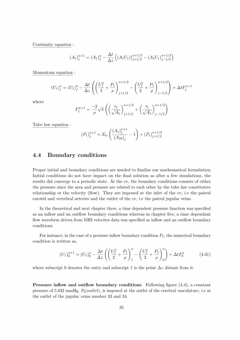
Continuity equation :

(A1)n+1j = (A1)nj −

∆t∆z

((A1U1))n+1/2

j+1/2 − (A1U1)n+1/2j−1/2

)

Momentum equation :

(U1)nj = (U1)nj −∆t∆z

(U21

2 + P1ρ

)n+1/2

j+1/2−(U2

12 + P1

ρ

)n+1/2

j−1/2

+ ∆tFn+1j

whereFn+1j = −2

ρ

√π

((τ1√A1

)n+1/2

j+1/2+(

τ1√A1

)n+1/2

j−1/2

)

Tube law equation :

(P1)n+1j = Elc

((A1)n+1

j

(A10)j− 1

)+ (Ps)n+1/2

j+1/2

4.4 Boundary conditions

Proper initial and boundary conditions are needed to finalize our mathematical formulation.Initial conditions do not have impact on the final solution as after a few simulations, theresults did converge to a periodic state. At the cv, the boundary conditions consists of eitherthe pressure since the area and pressure are related to each other by the tube law constitutiverelationship or the velocity (flow). They are imposed at the inlet of the cv, i.e the pairedcarotid and vertebral arteries and the outlet of the cv, i.e the paired jugular veins.

In the theoretical and next chapter three, a time dependent pressure function was specifiedas an inflow and an outflow boundary conditions whereas in chapter five, a time dependantflow waveform driven from MRI velocites data was specified as inflow and an outflow boundaryconditions.

For instance, in the case of a pressure inflow boundary condition P1, the numerical boundarycondition is written as,

(U1)n+10 = (U1)n0 −

∆t∆z

((U2

12 + P1

ρ

)n1−(U2

12 + P1

ρ

)n0

)+ ∆tFn0 (4.31)

where subscript 0 denotes the entry and subscript 1 is the point ∆z distant from it.

Pressure inflow and outflow boundary conditions Following figure (4.4), a constantpressure of 5.832 mmHg, Pb(outlet), is imposed at the outlet of the cerebral vasculature, i.e atthe outlet of the jugular veins number 33 and 34.

35

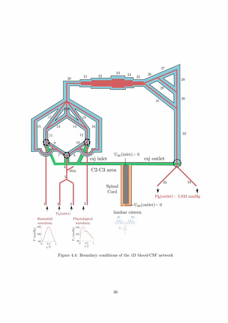
33 34

32

1

3 4 2

5

1

66bis

10

11 12

13 1415

17 18

19

20 21 22

9

31 30

29

28

27

26252423

16

7 8

Spinal Cord

lumbar cistern

csj inlet csj outlet

C2-C3 area

Sinusoidal waveform

Physiological waveform

Pb(intlet)

Pb(outlet)= 5.832 mmHg

Usc(inlet)= 0

Usc(outlet)= 0

R1 R2

Cl

Figure 4.4: Boundary conditions of the 1D blood-CSF network

36

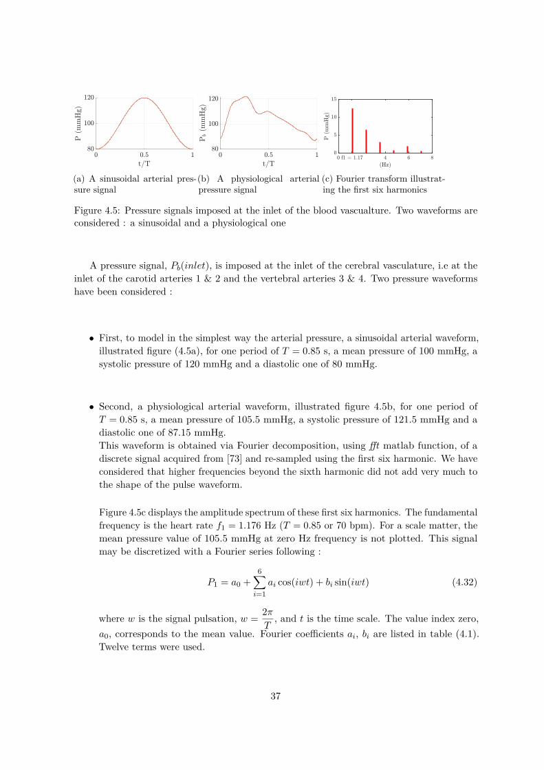
(a) A sinusoidal arterial pres-sure signal

(b) A physiological arterialpressure signal

(c) Fourier transform illustrat-ing the first six harmonics

Figure 4.5: Pressure signals imposed at the inlet of the blood vascualture. Two waveforms areconsidered : a sinusoidal and a physiological one

A pressure signal, Pb(inlet), is imposed at the inlet of the cerebral vasculature, i.e at theinlet of the carotid arteries 1 & 2 and the vertebral arteries 3 & 4. Two pressure waveformshave been considered :

• First, to model in the simplest way the arterial pressure, a sinusoidal arterial waveform,illustrated figure (4.5a), for one period of T = 0.85 s, a mean pressure of 100 mmHg, asystolic pressure of 120 mmHg and a diastolic one of 80 mmHg.

• Second, a physiological arterial waveform, illustrated figure 4.5b, for one period ofT = 0.85 s, a mean pressure of 105.5 mmHg, a systolic pressure of 121.5 mmHg and adiastolic one of 87.15 mmHg.This waveform is obtained via Fourier decomposition, using fft matlab function, of adiscrete signal acquired from [73] and re-sampled using the first six harmonic. We haveconsidered that higher frequencies beyond the sixth harmonic did not add very much tothe shape of the pulse waveform.

Figure 4.5c displays the amplitude spectrum of these first six harmonics. The fundamentalfrequency is the heart rate f1 = 1.176 Hz (T = 0.85 or 70 bpm). For a scale matter, themean pressure value of 105.5 mmHg at zero Hz frequency is not plotted. This signalmay be discretized with a Fourier series following :

P1 = a0 +6∑i=1

ai cos(iwt) + bi sin(iwt) (4.32)

where w is the signal pulsation, w = 2πT

, and t is the time scale. The value index zero,a0, corresponds to the mean value. Fourier coefficients ai, bi are listed in table (4.1).Twelve terms were used.

37

R1 R2

CPin PoutPc

Qin Qout

Qc

Figure 4.6: Three elements R1R2Clw Windkessel model

Coefficient Value (mmHg)a0 105.5a1 -6.122b1 10.54a2 -5.025b2 3.867a3 -2.815b3 -0.7914a4 -0.5171b4 0.5097a5 -1.846b5 0.1619a6 -0.3149b6 -0.4563

Table 4.1: Mean value, a0 and Fourier coefficients ai, bi, i = 1, 2, ..., 6 of (4.32) which capturesthe arterial pulsation

The lumbar terminal three elements Windkessel model A zero-dimensional (0-D)approach model governed by ordinary differential equations is used to relate pressure to flowat the outflow of the lumbar cistern using a three elements Windkessel model described infigure (4.6) where the proximal resitance R1 is introduced to absorb the incoming waves andreduce artificial wave reflections. It corresponds to the characteristic impedance Zl of lumbarvessel to match the propagation of forward travelling waves and defined as,

cl =√Elu

ρb, Zl = ρ

clA0l

where cl is the intrinsic lumbar segment wall wave speed, ρb the CSF density, Elu the lumbarsegment elastic modulus and A0l the lumbar segment cross sectional area at zero transmuralpressure.

In the analogous electrical circuit described figure (4.6), Qin, Qout defines respectivelythe input flow and output flow rate due to proximal resistance R1 and distal resistance R2

38

whereas Qc defines the flow rate of the capacitance C, Pin, Pout and Pc are respectively theinlet pressure, output pressure and capacitance pressure. The inlet and output flows Qin andQout may be described following Ohm’s low as,

Qin = Pin − PcR1

, Qout = Pc − PoutR1

(4.33)

Kirhoff’s law states that Qin = Qc +Qout and finally the capacitance pressure is defined as,

dPcdt

= QcC

(4.34)

A first order time discretization of the previous set of equations is written as,

Ain = AL0 −∆t∆x

((AU)nL − (AU)nL−1

), (4.35)

Pin = El(Ain

A0in − 1), (4.36)

Qnin = Pin − Pcn

R1 , (4.37)

Qnout = Pcn − PoutR2 , (4.38)

Pcn+1 = Pcn + ∆t Qnin

Qnout, (4.39)

Qn+1in = Pin − Pcn+1

R1 , (4.40)

Uin = Qn+1in /Ain (4.41)

where Pout is a constant pressure that was assumed equal to a mean intracranial pressure of10 mmHg and Pcn = 0 at the inital time step n=1.

4.5 Branching conditions

The 1D craniospinal model is characterized by the presence of branching. In this section, wewill address the problem of accounting for interface conditions.

Several configurations are found in the geometry structure as modeled in figure (4.4) anddetailed in B such as,

• A bifurcation of vessels, when a single (or coaxial) vessel bifurcates into two single (orcoaxial vessels). For instance, between vessels 25, 26 and 31.

• A junction of vessels occurs when two single (or coaxial) vessel join into one single ( orcoaxial) vessel. For instance, between vessels 31, 30 and 32.

• Finally an enlargement (or reduction) of vessels, defines a branching between two single

39

(or coaxial) vessels of different cross-sectional areas. For instance, between vessels 20and 21.

The flow in a branching configuration is intrinsically three-dimensional; yet it may stillbe represented by means of a 1D model. In a first stage we simplify the actual geometricstructure by imposing that the branching is located exactly at one point and neglecting theeffect of branching angles.

In the following formulation, we will only address the case of a widening or a narrowing oftubes. However, the methodology employed here is extended as well to the cases of a junction,enlargement or reduction of vessels in a single or coaxial configuration and moreover to thebranching interfaces between the cerebral vasculature, the cranio-cervical junctions and thespinal subarachnoid spaces.

The following subscripts are used : 1 for the interior tube and 2 for the exterior tube.

case 1 : A widening or a narrowing of tubes

Interior tube

•

a

•

b

•

c

•

d

For the interior tube, the jump conditions between the points b and c are :

(AU)1b = (AU)1c (4.42)

P1b = P1c (4.43)

P1b = El1b

(A1bA01b

− 1)

+ P2b (4.44)

P1c = El1c

(A1cA01c

− 1)

+ P2c (4.45)

The equations (4.42) and (4.43) express the conservation of mass and pressure between b et c.We have 6 unkown terms and and we only have 4 equations. To complete this system, theconservation of mass equation was derived between a et b then between c et d :∫ b

a

∂A1∂t

dx+ (AU)n+11b − (AU)n+1

1a = 0 (4.46)

∫ d

c

∂A1∂t

dx+ (AU)n+11d − (AU)n+1

1c = 0 (4.47)

40

The derivatives and integrals are evaluated using the difference finite method and the trape-zoidal rule. Therefore, we obtain :

∆xa2∆ta

(An+1

1a −An1a +An+1

1b −An1b

)+ (AU)n+1

1b − (AU)n+11a = 0 (4.48)

∆xd2∆td

(An+1

1d −An1d +An+1

1c −An1c

)+ (AU)n+1

1d − (AU)n+11c = 0 (4.49)

Using the equations (4.43), (4.44) and (4.45) and the pressure jump conditions of the exteriortubes (P2b = P2c), we obtain :

A1c = El1bEl1c

A01cA01b

A1b +A01c

(1− El1b

El1c

)(4.50)

By writing equation (4.50) for An+11c and An1c, we obtain:

An+11c −A

n1c = El1b

El1c

A01cA01b

(An+11b −A

n1b) (4.51)

Put,

Ra =( ∆xa

2∆ta

), Rd =

( ∆xd2∆td

), K1bc = El1b

El1c

A01cA01b

By replacing (4.51) in equation (4.49) and by taking into account the conservation of massequation (4.42), we obtain by adding (4.48) and (4.49) :

An+11b =An1b + (AU)n+1

1a − (AU)n+11d −Ra(A

n+11a −An1a)−Rd(A

n+11d −An1d)

Ra +RdK1bc(4.52)

Using the same procedure, we obtain Un+11b by subtracting the equation (4.49) from the

equation (4.48).

Un+11b =(AU)n+1

1a + (AU)n+11d −Ra(A

n+11a −An1a) +Rd(An+1

1d −An1d)2An+1

1b

−(Ra −RdK1bc)(An+1

1b −An1b)2An+1

1b(4.53)

4.5.0.1 Exterior tube

For the exterior tube, the jump conditions between the points b and c are :

((A2 −A1)U2)b = ((A2 −A1)U2)c (4.54)

P2b = P2c (4.55)

P2b = El2b

(A2bA02b

− 1)

(4.56)

41

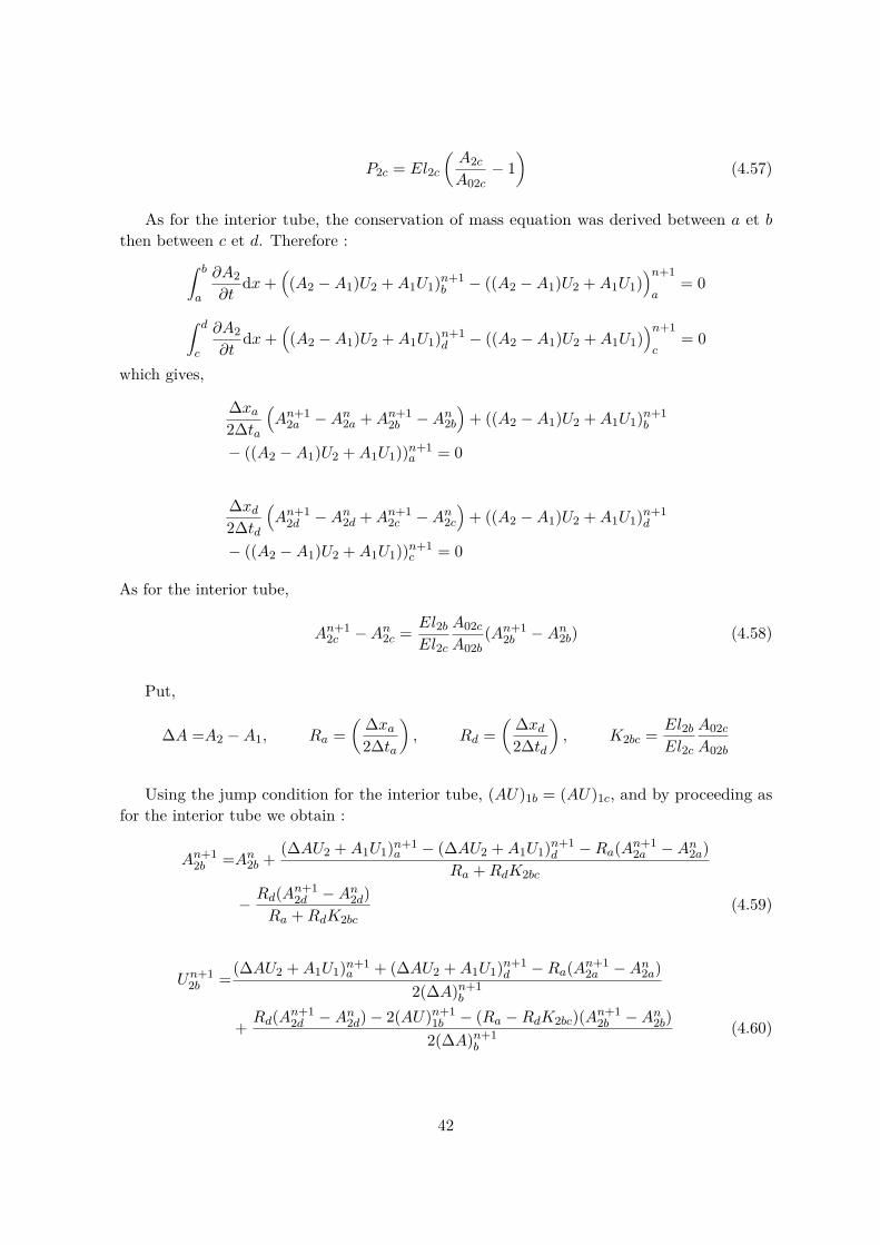
P2c = El2c

(A2cA02c

− 1)

(4.57)

As for the interior tube, the conservation of mass equation was derived between a et bthen between c et d. Therefore :∫ b

a

∂A2∂t

dx+((A2 −A1)U2 +A1U1)n+1

b − ((A2 −A1)U2 +A1U1))n+1

a= 0

∫ d

c

∂A2∂t

dx+((A2 −A1)U2 +A1U1)n+1

d − ((A2 −A1)U2 +A1U1))n+1

c= 0

which gives,

∆xa2∆ta

(An+1

2a −An2a +An+1

2b −An2b

)+ ((A2 −A1)U2 +A1U1)n+1

b

− ((A2 −A1)U2 +A1U1))n+1a = 0

∆xd2∆td

(An+1

2d −An2d +An+1

2c −An2c

)+ ((A2 −A1)U2 +A1U1)n+1

d

− ((A2 −A1)U2 +A1U1))n+1c = 0

As for the interior tube,

An+12c −A

n2c = El2b

El2c

A02cA02b

(An+12b −A

n2b) (4.58)

Put,

∆A =A2 −A1, Ra =( ∆xa

2∆ta

), Rd =

( ∆xd2∆td

), K2bc = El2b

El2c

A02cA02b

Using the jump condition for the interior tube, (AU)1b = (AU)1c, and by proceeding asfor the interior tube we obtain :

An+12b =An2b + (∆AU2 +A1U1)n+1

a − (∆AU2 +A1U1)n+1d −Ra(An+1

2a −An2a)Ra +RdK2bc

−Rd(An+1

2d −An2d)Ra +RdK2bc

(4.59)

Un+12b =(∆AU2 +A1U1)n+1

a + (∆AU2 +A1U1)n+1d −Ra(An+1

2a −An2a)2(∆A)n+1

b

+ Rd(An+12d −An2d)− 2(AU)n+1

1b − (Ra −RdK2bc)(An+12b −An2b)

2(∆A)n+1b

(4.60)

42

We notice that the parameters U , P and A of the two tubes are coupled.Therefore, first we could calculate A2b using the equation (4.59).From the equation (4.56), we obtain P2b.From the equation (4.55), we obtain P2c.From the equation (4.57), we obtain A2c.From the equation (4.52), we obtain A1b.From the equation (4.53), we obtain U1b.From the equation (4.44), we obtain P1b.From the equation (4.43), we obtain P1c.From the equation (4.45), we obtain A1c.From the equation (4.42), we obtain U1c.From the equation (4.60), we obtain U2b.From the equation (4.54), we obtain U2c.

43

Chapter 5

Blood-CSF coupling effect on thecerebral vasculature and CSF

dynamics

Sommaire5.1 Introduction . . . . . . . . . . . . . . . . . . . . . . . . . . . . . . . . . . 455.2 An arterial sinusoidal waveform . . . . . . . . . . . . . . . . . . . . . . . 465.3 Effect of varying the confinement and assessment of CSF viscosity . 535.4 Effect of the cranio-spinal compliance . . . . . . . . . . . . . . . . . . . 555.5 Effect of varying the cranial subarachnoid spaces compliance . . . . . 575.6 Effect of varying the spinal subarachnoid spaces compliance . . . . . 585.7 An arterial physiological waveform . . . . . . . . . . . . . . . . . . . . . 605.8 Conclusion . . . . . . . . . . . . . . . . . . . . . . . . . . . . . . . . . . . 61

5.1 Introduction

This chapter first aims to investigate and analyze the main effects of coupling blood and CSFflow on pulse wave propagation. Several aspects are highlighted. During the first section, weanalyse the effect of CSF pulsations on blood dynamics. Thus, two models are being compared,a model accounting for CSF coupling and a model lacking CSF coupling. In the second section,we investigate the effect of varying the CSF confinement or CSF volume. Finally, the thirdsection elucidates the role played by the cranial and spinal CSF compartments complianceduring vascular brain expansion.

General considerations The following outcomes will be considered:

• The mean pressure, P , and mean flow, Q.

• The pressure peak to peak or pulse pressure, Ppp, defined as the difference between themaximum and minimum pressure amplitudes. Usually for clinicians, the term PulsePressure accounts for the difference between the systolic and diastolic blood pressure.

45

• The peak flow, Qp as ’p’ for peak.

• The stroke volume, Sv, defined as the amount of blood or CSF displaced at each cardiaccycle.

• The pulse wave velocity (PWV) defined as the velocity at which a pulse wave propagatesfrom site to site.

• The phase-lag. As we made the assumption that the driving force behind CSF pulsationsis the arterial input, we used the carotid artery flow as the reference against which wecompared blood and CSF flow. It is computed as the difference between two analogouspoints of two signals, divided by the total period of the wave. It is expressed in percentageof the cardiac cycle %cc. The phase lag between the internal carotid and jugular peakflows or cervical CSF flows reflects the pulse wave velocity through the vessels betweenthese 2 sites and can be used as a measure of vascular or CSF system compliance.

Remarque 5.1Recall that the following subscripts are used : ’c-m’ refers to the curent model, the coupledblood-CSF model, in contrast to ’u-m’ for the uncoupled blood model, i.e a model lacking CSFcoupling. ’cv’ refers to the cerebral vasculature. As for the CSF system, csas refers to thecranial subarachnoid spaces and ssas for spinal subarachnoid spaces.

5.2 An arterial sinusoidal waveform

Boundary conditions First a sinusoidal input pressure with an apporpriate waveformis used to model in the simplest way the arterial pressure and reproduce the physiologicalconditions. The results of a physiological arterial waveform will be displayed in section 5.7. Itfeatures a systolic blood pressure of 120 mmHg, a diastolic blood pressure of 80 mmHg, and aperiod of T=0.85 s. However, temporal evolution results will be displayed in a dimensionlesstime (t/T). The arterial pressure was imposed at the inlet of the cerebral vasculature, i.e thepaired carotids and vertebral arteries whereas a constant output pressure of 5.832 mmHg wasassumed at the outlet of the jugular veins 33 & 34.

Computations were performed using the following values of the CSF network mechanicalproperties:a cranial CSF confinement at zero transmural pressure of λ0cb = 0.7 It correspondsto a total CSF volume of 130 mL which lies in the range of MRI measured CSF volumes. Thecranial and spinal dura mater were assigned an elastic modulus of El = 107 mmHg whichyielded to a cranial sas compliance of 0.02 mL/mmHg and a spinal sas compliance of 0.01mL/mmHg.

Arterial, venous and Spinal CSF flow Figure (5.1) displays pressure and flow of thecarotid artery, the jugular vein and the cervical CSF flow. Table (5.1) details the maximum,mean and minimum amplitudes of pressure and flow. The model predicted a global cerebral

46

(a) Carotid artery P (b) Carotid artery Q (c) Jugular vein P (d) Jugular vein Q

(e) CSF C2-C3 P (f) CSF C2-C3 Q

Figure 5.1: Pressure and flow of the carotid artery, the jugular vein and the cervical CSF flowfor a sinuoidal waveform

blood flow of 10.1 cm3/s which corresponds for an average brain of 1400 g to a cerebral bloodvolume (CBV) of 43.2 mL.100 g−1.min−1 which is within the normal range of CBF [61].

The model predicts a pulsatile spinal CSF flow with zero net flow, a CSF caudal flowduring systole and a CSF rostral flow during diastole, a peak flow of 0.5 mL/s and a strokevolume of 0.2 mL which is in accordance with previous MRI observations [2, 24, 16, 5].

Inlet carotid ar-teries 1 & 2

Inlet vertebralarteries 3 & 4

Outlet jugularveins 33 & 34

Cervical CSF

Pmax, Pmean, Pmin 120/100/80 120/100/80 6.2/5.8/6 10.5/7.8/5(mmHg)

Qmax, Qmean, Qmin 4.7/3.4/2.1 2.3/1.6/0.8 5.3/4.2/3.1 0.5/10−6/-0.5(mL/s)

Table 5.1: Maximum, mean and minimum pressure-flow amplitudes of carotid artery 1, jugularvein 33 and cervical CSF for a sinusoidal arterial waveform

Reynolds number and Womersley number Reynolds and Womersley numbers are thetwo nondimensional parameters used to specify pulsatile flow. The Reynolds number relatesthe ratio of inertial to viscous forces. Hereby, we considered the peak or systolic Reynolds Rpnumber (subscript p as peak). It was defined by,

Rp = ρDupµ

(5.1)

47

It is based on the fluid peak velocity up, the fluid density ρ and kinematic voscosity µ. Thecharacteritic dimension D was either the diameter for a circular tube or the hydraulic diameterfor an annular tube. The hydraulic diameter being computed as 4.Area/perimeter. Forthe cerebral vasculature, when vessels were regrouped into equivalent tubes such as the pialarteries or the microcirculation, the peak Reynolds number was computed based upon thereal section and not the equivalent section.

Figure 5.2a displays the peak Reynolds number for the cv (in red) and the cranial sas (inblue). The maximum peak Reynolds number, Rep = 400, for the cerebral vasculature wasobserved at the large carotid arteries (vessel number 1 and 2). The regrouped vessels such asthe pial network (vessel 21), the intracerebral arteries (vessel 22) and the microcirculation(number 23) displayed, although not visible, low Reynolds numbers.

Our model predicts cranial CSF flow Reynolds number of less than 50. Gupta et al. [29]have performed 3D CFD simulations and reported Reynolds number of 114 and 20 in theanterior and cranial SAS. Howden et al. observed using CFD simulations a maximum Reynoldsnumber of 15 in the ventricular system. Pahlavian et al. [53] and Loth at al. [42] performedrespectively 3D and 2D CFD simulations in the cervical spine and reported respectively peakReynolds number of 187 and 201. The current model predicts at the C2-C3 region a Reynoldsnumber of 146 which is in agreement with the latter studies.

The Womersley number quantifies the transient inertial forces in proportion to viscouseffects. It was defined as,

Wo = D

2

√ρω

µ(5.2)

where w = 2π/T is the cardiac pulsation and D is either the diameter for a circular tube orthe hydraulic diameter for an annular tube. Figure 5.2b displays the Womersley number ofthe cv (in red) and the cranial sas (in blue). Recall that for a circular tube, the Poiseuillevelocity hypothesized in our mathematical formulation is theoretically only valid for a steadyflow. However, it can be used as a first approximation for small values of Womersley numbers.For the cv and the cranial sas, the largest value of Wo is about 11 for the transverse sinus(number 32) and 4 for the annular cranial sas enclosing the transverse sinus. Their effects maybe considered negligible relative to the whole network. Loth at al. [42] have quantified CSFflow Womersley numbers and has found it varying between 5 and 17. In this study, [42] hasfound the greatest Womersley number in the cervical and lumbar sas.

Recall that in our study, for a simplification matter, we have assumed a quasi-steady fowapproximation. This approximation has led to assume a parabolic velocity profile in orderto approximate the wall shear stress. The validity of this approximation in the annular andcircular spinal subarachnoid space (SSS) is discussed in the undergoing publication of annexeC. In summary, the wall shear stress was found depending on two parameters, the Womersleynumber and the width of the annular SSS. We found that the more the annular SSS is narrow,the more the average wall shear stress of a quasi-steady fow approximation is valid.

48

(a) Reynolds number

(b) Womersley number

Figure 5.2: Dimensionless Reynolds and Womersley number of the cerebral vasculature (cv)and the cranial subarachnoid spaces (csas)

Damping mechanisms due to CSF coupling For every organ in the human body, thearterial Windkessel properties of the vasculature are known to play a significant role in bufferingarterial pulsations through elasticity of the blood vessels [71, 13]. In the brain, the arterialWinkessel mechanism is thought to buffer acute arterial pulsations, which may be harmfulto the cerebral bed capillary network, to a more steady stream of blood. A physiologicallyimportant aspect of pulsatility in the cranium is the Windkessel effect, the dissipation ofarterial pulsatility rendering capillary blood flow nearly pulseless. Moreover, Wagshul et al. [43]has suggest that due to abnormal compliance of patients with chronic hydrocephalus, CSF mayalso play a role as the brain’s shock absorber by allowing dissipations of intracranial pulsationsbefore they are able to reach the microcirculation. Later, the authors have performed changesin ICP in dogs and have hypothesized that the intracranial compartements appear to act as anotch filter (Band reject filter) attenuating the frequency of the heart rate relative to otherfrequencies [22, 74].

Pressure and flow of the cv can be divided following two groups: on the one hand thearterial network and on the other hand the more compliant venous network. Hereby, arterialvessel number 21 equivalent to the arterioles and venous vessel number 31 equivalent to thetransverse sinuses were chosen respectively as representative of both the arterial and thevenous network. A similar strategie was performed for the subarachnoid spaces. On the onehand, the cranial sas coaxial to the arterial system and on the other hand, the cranial sascoaxial to the venous system.

Figure (5.3) portrays from left to right the temporal distribution during a dimensionless

49

(a) Pressure (b) Flow (c) Area (d) Pressure (e) Flow (f) Area

Figure 5.3: From left to right : Pressure, flow and relative area temporal evolution of arterioles(vessel 21) followed by the transverse sinus (vessel 31). c-m: coupled model, u-m: uncoupledmodel

period (t/T) of pressure P , flow Q and relative section ((A(t)−A0)/A0)) of arterioles vessel21 followed by the transverse sinuses 31. Solid lines denotes the current blood-CSF coupledmodel (c-m) and dashed lines refers to the uncoupled blood model (’u-m’).

During a cardiac cycle blood pressure rises in systole and decreases in diastole (see subfigure(a) and (d)). Due to the pressure gradient or CPP, blood flow is positive and closely followsthe pressure waveform (see subfigure (b) and (e)). Finally, the model predicts blood smallarea variation (see subfigure (c and (f)).

In the c-m model, CSF pulsations were found to cause a dampening and a phase lag ofpressure and section relative to the uncoupled model u-m. The dampening was found toimpact the maximum and the minimum amplitude. However, mean flow and pressure werenot affected which implies that the maximum amplitude dampening is equal to the minimumamplitude dampening. Moreover, in the c-m model note that CSF flow causes compression ofthe venous vessels (see (f)).

Figure (5.4) displays the attenuation values of peak flow, %Qp, and peak to peak pressure,%Ppp accross the cv. Recall that the arterial network designates vessel 1 to 22 and the venousvessels designates vessels 24 to 34. Vessel 23 being the microcirculation. For example, thearterial system pulse pressure (vessel 1 or 2) was found decreased by less than ∼ 2% whereasthe venous system pulse pressure was found decreased by more than ∼ 6%. CSF flow causesmore reduction to the compliant venous network than the arterial network.

Time delay of the cv relative to the carotid artery flow is displayed in figure (5.5) for thec-m and the u-m models. CSF pulsations slightly affect the phase lag in arteries whereasthere is a significant reduced phase lag in the venous system. Note that the jugular vein peakflow was found to occur earlier due to confinement and mainly to the great cranial elastance.Hence, CSF coupling allows a faster transmission of the arterial pulsations to the venousvessels via the cranial subarachnoid space.

Cranial CSF flow Figure (5.6) portrays the temporal distribution during a dimensionlessperiod (t/T) of flow, pressure and relative section of cranial subarachnoid spaces coaxialto the arterioles (number 21) and the transverse sinuses (number 31). Recall that bloodand CSF pressure are coupled using the tube law equation established in section 4.2.3

50

(a) Blood flow amplitude variation

(b) Blood peak to peak pressure variation

Figure 5.4: Blood peak flow and blood peak to peak pressure damping accross the coaxialcerebral vasculature

Figure 5.5: Phase lag to carotid artery flow. c-m: coupled-model, u-m: uncoupled-model

51

(a) Pressure (b) Flow (c) Area (d) Pressure (e) Flow (f) Area

Figure 5.6: From left to right, pressure, flow and relative area temporal evolution of cranialsas coaxial to arterioles (vessel 21) and coaxial to transverse sinus (vessel 31)

Pc = Pb − (El)b(Ab/(A0)b − 1) where Pc is the CSF pressure, Pb is the blood pressure, (El)b isthe blood vessel elastance, Ab is the varying cross sectional area and (A0)b is the cross-sectionalarea at zero transmurale pressure. Hence, cranial CSF pressure closely follows blood pressurewaveform (see subfigure (a) and (d). Subfigures (b) and (e) displays cranial CSF flow. Themodel predicts a mean cranial CSF flow, in green dashed lines, close to zero implying thatcranial CSF flow is pulsatile flowing forwards and backwards during a cardiac cycle. Finally,the model predicts small cranial sas area variation, subfigure (c) and (f).

Pressure drop accross the cerebral vasculature and intracranial pressure Recallthat the cerebral vaculature is composed of 34 vessels where each blood vessel starting fromthe basilar artery bifurcation (vessel 7 & 8) to the transverse sinuses (vessel 32) is surroundedby the cranial subarachnoid spaces. Figure (5.7a) portrays the predicted mean pressure of thecerebral vasculature (cv). Figure shows that blood pressure drops unevenly as blood travelsfrom arteries to arterioles, capillaries, venules, and veins, and encounters greater resistance.However, the site of the most precipitous drop, and the site of greatest resistance occurs atthe arterioles (vessel 22). Arterioles admits a greatest elastance than previous vessels, a largercross sectional area but individually a smaller diameter. This means more of the blood is incontact with the vessel wall, and therefore resistance increases. This explains why vasodilationand vasoconstriction of arterioles play more significant roles in regulating blood pressure thando the vasodilation and vasoconstriction of other vessels.

Figure (5.7b) portrays the predicted maximum, mean and minimum pressure of the csas(cv). CSF mean pressure remains roughly constant at about 8 mmHg. Cranial CSF peak topeak pressure are small despite large arterial peak to peak pressure of 40 mmHg. The CSFpressure steadiness is due to the availability of the compliant spinal canal to receive CSF. Themodel supports the theory of the spinal canal’s role to attenuate CSF pressure amplitudes.

Blood and CSF fluids variations Figure (5.8) portrays volume temporal distribution ofthe total coaxial blood vessels, the arterial system, the venous system, the cranial and thespinal CSF. First of all, the brain vasculature volume, subfigure (a), was found to expandslesser due to CSF presence. Indeed, as the arterial volume variation, subfigure (b), is slightlyaffected by CSF pulsations, it is mainly the venous volume, subfigure (c) which is greatlyattenuated. Moreover, during systole, i.e the first half-period, due to CSF presence the model

52

(a) Mean pressure of the cerebral vasculature (cv)

(b) Max., mean and min. of cranial CSF pressure

Figure 5.7: (a) Mean pressure of the cerebral vasculature (cv). (b) Max., mean and min. ofcranial CSF pressure

predicts a compression of the venous system instead of dilatation in a model lacking CSFcoupling.

Coaxial blood vessels were found to inflate and deflate by 0.26 mL, the same amount ofspinal CSF stroke volume of 0.26 mL reported previously.

To explain fluids exchange between blood and CSF between the cranial and spinal vaults,their volumes were scaled and plotted in subfigure 5.8f. During the first half-period, arterialvolume expansion is regulated by both venous volume and cranial CSF volume compression.The decrease in intracranial CSF volume is made possible by means of displacement of cranialCSF into the spinal sas which can expand by the compliance of the dural sac.

Our model supports the theory that during systole, the arterial volume expansion isregulated by two complementary damping mechanisms which are the venous compression andthe spinal CSF volume increase.

5.3 Effect of varying the confinement and assessment of CSFviscosity

This section explores cranial CSF confinement effect on blood and CSF flow dynamics. Amentionned previously, the cranial CSF confinement is a dimensionless number which relatesa blood vessel section to a cranial sas section at zero transmural pressure. λcb, may range

53

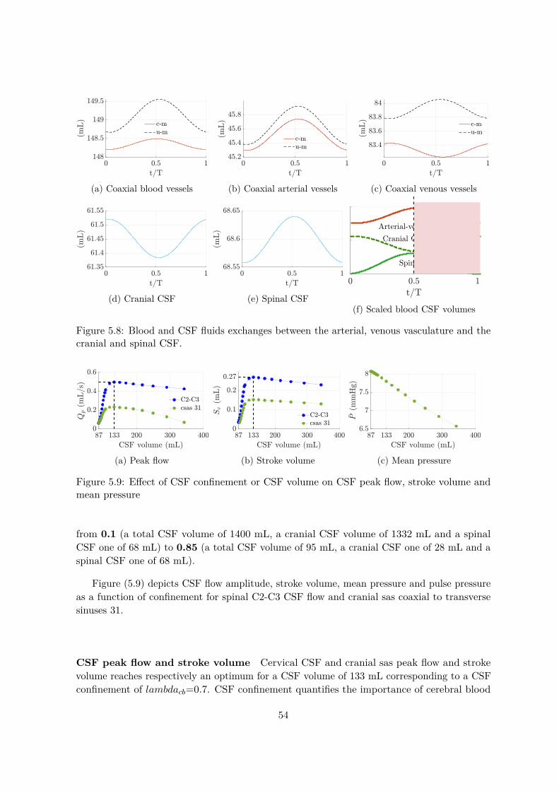
(a) Coaxial blood vessels (b) Coaxial arterial vessels (c) Coaxial venous vessels

(d) Cranial CSF (e) Spinal CSF

Spinal CSF volume

Cranial CSF volumeArterial-venous volume

(f) Scaled blood CSF volumes

Figure 5.8: Blood and CSF fluids exchanges between the arterial, venous vasculature and thecranial and spinal CSF.

(a) Peak flow (b) Stroke volume (c) Mean pressure

Figure 5.9: Effect of CSF confinement or CSF volume on CSF peak flow, stroke volume andmean pressure

from 0.1 (a total CSF volume of 1400 mL, a cranial CSF volume of 1332 mL and a spinalCSF one of 68 mL) to 0.85 (a total CSF volume of 95 mL, a cranial CSF one of 28 mL and aspinal CSF one of 68 mL).

Figure (5.9) depicts CSF flow amplitude, stroke volume, mean pressure and pulse pressureas a function of confinement for spinal C2-C3 CSF flow and cranial sas coaxial to transversesinuses 31.

CSF peak flow and stroke volume Cervical CSF and cranial sas peak flow and strokevolume reaches respectively an optimum for a CSF volume of 133 mL corresponding to a CSFconfinement of lambdacb=0.7. CSF confinement quantifies the importance of cerebral blood

54

section (volume) to cranial CSF section (volume),

volume(blood)volume(csf) = λcb

1− λcb(5.3)

In cranial sas 31, as λcb reaches towards 0.1 or as cranial CSF volume increases, cerebral bloodvolume is assumed to drag a great amount of cranial CSF volume, and consequently CSF flowdrops. Whereas, as λcb reaches towards 0.9, or as cranial CSF volume decreases, there is moreCSF contacting the vessel wall, thus higher friction and higher resistance and subsequentlydecreasing flow. This demonstrates the existence of a confinement at which CSF flow andstroke volume are maximal. A more theoretical investigation requires a closer look to themomentum conservation equation for an annular tube. Recall that the momentum equationof an annular tube was defined as,

ρ∂Q2∂t

+ ρ∂

∂z

(Q2

2A2 −A1

)+ (A2 −A1)∂P2

∂z= 2π(R2τ2 −R2τ12) (5.4)

where the first term of the left hand side ∂Q2/∂t represents the inertial forces, the secondterm portrays the convective term ∂(Q2

2/(A2 − A1))/∂z, the third term (A2 − A1)∂P2/∂z

represents the pressure term and finally the right hand side displays the viscous term 2π(R2τ2−R2τ12). Figure (5.10) depicts temporal evolution of these four terms in cranial sas coaxial totransverse sinus 31 for three confinement values λcb =0.3, 0.5 and 0.7.

As displayed in figure (5.10) for a confinement of λcb =0.3, inertial forces (in blue line)dominate the viscous forces (in green line). For a confinement of λcb =0.5, inertial and viscousforces are of the same order of magnitude and finally for a confinement of λcb =0.7, viscousforces greatly dominates inertial forces. To finally assess the imbalance between inertial andviscous forces, figure (5.11) compares CSF maximum flow evolution for a viscous and nonviscous CSF model. As expected, when considering CSF viscous, CSF maximum flow drops atlower confinement due to higher friction.

Loth et al. [42] numerical and experimental study showed that the pulsatile flow of theCSF in the spinal sas is characterised by relatively dominated inertia effects mainly near thecervical and lumbar area, i.e where spinal sas are the largest. However, as sas gets smaller,viscous effect increases and challenges inertia effect suggesting the need to account for CSFviscosity at least in small annular spaces as the cranial sas. Finally, it is important to notethat the overall contribution of CSF viscosity is not negligible in the cranial sas and thereforemay affect spinal CSF.

5.4 Effect of the cranio-spinal compliance

Recall that cerebral compliance is provided mainly by the intracranial venous system, theextracellular spaces and the CSF system. Intracranial compliance (ICC) represents the changein volume (∆V ) per unit change in pressure (∆P ), and is exactly the inverse of elastance. In

55

(a) λcb=0.3 (b) λcb=0.5 (c) λcb=0.7

Figure 5.10: Evolution during a cycle of the conservation of momentum terms for threedifferent confinement λcb=0.3, 0.5 and 0.7 where Tq,t = ρdQ2/dt, Tp,z = (A2 − A1)dp/dz,Tq2,a,z = d(Aanr ∗Q2)/dz and Tf = 2π(R2τ2 −R1τ12).

Figure 5.11: Effect of CSF viscosity on cranial CSF peak flow

other words, ICC determines the ability of the intracranial compartment to accommodate anincrease in volume without a large increase in pressure. In this section, we investigate theeffect of the craniospinal compliance of subarachnoid spaces on blood and CSF pulsations.Recall that the elastic Young modulus differs from the elastance which is the reciprocal of thecompliance.

In order to allow analogy between the cranial and the spinal compliance, their respectiveelastic Young modulus will be expressed in terms of a volumetric compliance using the tubelaw equation. Morevoer, the three elements Windkessel compliance will be tuned in order toequal the compliance of the spinal dura mater.

Intrinsic relationship between a vessel compliance and the elastic modulus of itswall Recall that a vessel compliance expressed in (mL/(dyne/cm2) is defined as,

C = ∆V/∆P (5.5)

Moreover, in our mathematical formulation of the tube law equation, a linear relation wasassumed beetween the transmural pressure Pt and the varying vessel cross-sectional area A(or vessel volume V ) defined as,

Pt = El(A

A0− 1) = El(

V

V0− 1) (5.6)

56

where A0 and V0 are respectively the cross sectional area volume at zero transmural pressureand El is the Young modulus expressed in dyne/cm2.

By combining the two previous equation (5.5) and (5.6), one might write,

∆Pt = El∆VV0

,∆V∆Pt

= V0El, Cl = V0

El(5.7)

Using the latter equation, the cranial sas compliance will be defined as Clc = V0c/Elc

where Elc is the cranial dura mater elastic modulus and V0c is the cranial CSF volume. In asimilar manner, the spinal sas compliance will be defined as Cls = V0s/Els where Els is thespinal dura mater elastic modulus and V0s is the spinal CSF volume. Finally, as mentionedpreviously, the 3 element Windkessel compliance was assumed to be identical to spinal sascompliance.

5.5 Effect of varying the cranial subarachnoid spaces compli-ance

In this section, we investigate the cranial subarachnoid spaces compliance effect on blood andCSF dynamics. CSF volume was assumed to be 215 mL divided into a cranial CSF volume of147 mL and a spinal CSF one of 68 mL which lie within the range of physiological CSF volumevalues [3, 63]. Usually, healthy physiological values of the Young elastic modulus of the duramater ranges between 600 mmHg and 5.104 mmHg as described previously in section 3.4.1.In this study, for a theoretical perspective and to account for extreme cases of either verycompliant or very rigid dura mater, the range of the dura mater elastic Young modulus wasextended. Therefore, the cranial sas elastic modulus Elc was taken varying between 75 mmHgand 7.5.104 mmHg which correponds to a cranial sas compliance varying between 0.002 and 2mL/mmHg. The spinal sas elastic modulus was assumed equal to 103 mmHg whic impliesa spinal compliance of 0.07 mL/mmHg. Finally, the 3 elements Winkessel compliance wasassumed equal to 0.07 mL/mmHg.

Figure (5.12) displays cranial and spinal mean pressure, peak flow and stroke volume asa function of the cranial sas compliance. Regarding venous flow, displayed (a) and (b), ascranial sas compliance decreases, CSF pulsations were found to dampen venous peak flow andpulse pressure. Whereas, as cranial sas increases, the effect of the constraint on the venousflow weakens, and consequently peak flow and pulse pressure increase and tend to convergetowards a model lacking CSF coupling.

The model predicts that decreasing intracranial compliance increases CSF mean pressure,pulse pressure and peak flow in the cranial and spinal vault. As demonstrated by several MRIstudies of pathological disorders, decreased intracranial compliance severly affects intracranialpressure. For example, a previous study by Alperin et al. [4] has provided evidence thatincreasing ICC compliance by means of decompression surgery in Chiari Malformations has

57

(a) Pressure peak to peak (b) Peak flow

(c) Mean pressure (d) Peak flow (e) Stroke volume

(f) Mean pressure (g) Peak flow (h) Stroke volume

Figure 5.12: Effect of intracranial compliance Cld on (working from top to bottom) venousflow, cranial CSF flow and spinal CSF flow

shown a great decrease in CSF pressure.

5.6 Effect of varying the spinal subarachnoid spaces compli-ance

In this section, we investigate the spinal subarachnoid spaces compliance effect on blood andCSF dynamics. CSF volume was assumed to be 215 mL divided into a cranial CSF volumeof 147 mL and a spinal CSF one of 68 mL. The spinal sas elastic modulus Elc was takenvarying between 37.5 mmHg and 7.5.104 mmHg which correponds to a spinal sas compliancevarying between 0.001 and 2 mL/mmHg. The cranial sas elastic modulus was assumed equal to7.5.104 mmHg which implies a cranial compliance of 0.002 mL/mmHg. Finally, the 3 elementsWinkessel compliance was assumed varying and equal to the spinal sas compliance.

Figure (5.13) displays cranial and spinal CSF mean pressure, peak flow and stroke volumeas a function of the spinal sas compliance. The curves distribution may be divided into twoparts: a high compliance part and a low compliance part. In the low compliance part, despite

58

(a) Pressure peak to peak (b) Peak flow (c) Pressure

(d) Pressure (e) Peak flow (f) Stroke volume

Figure 5.13: Effect of spinal dura mater elasic modulus Eld on cranial, spinal CSF and venousflow.

Figure 5.14: Spinal volumetric compliance effect on spinal CSF pulse wave velocity (pwv)

the increase in spinal compliance, cranial and cervical CSF display a plateau of pressure anda maximum followed by a plateau for peak flow and stroke volume. However, in the lowcompliance part, any small decrease in the spinal compliance elicit high increases in cranial andspinal pressure and consequently a decrease in cranial and spinal flow. This behaviour remindsthe presure-volume curve linking intracranial pressure to intracranial compliance. In the highcompliance part, spinal and cranial CSF pressure are steady, whereas as spinal compliancedecrease, CSF fails to play its buffering role, thus resulting in an increase of pressure andultimately a decrease of flow.

Figure (5.14) displays spinal CSF pulse wave velocity along the spinal sas between thecervical and the lumbar region. Spinal sas pwv was found to decrease under increasing spinalsas compliance. Moreover, the range of pulse wave velocity is in agreement with previous MRIstudies as Kalata et al. [36] where, in this study, a novel MR sequence was used to acquireunsteady spinal CSF velocity measurements during the cardiac cycle.

59

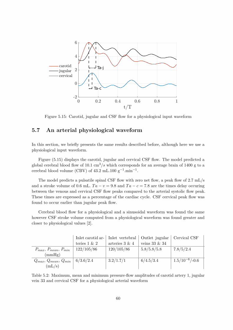
Ta-j

Ta-c

Figure 5.15: Carotid, jugular and CSF flow for a physiological input waveform

5.7 An arterial physiological waveform

In this section, we briefly presents the same results described before, although here we use aphysiological input waveform.

Figure (5.15) displays the carotid, jugular and cervical CSF flow. The model predicted aglobal cerebral blood flow of 10.1 cm3/s which corresponds for an average brain of 1400 g to acerebral blood volume (CBV) of 43.2 mL.100 g−1.min−1.

The model predicts a pulsatile spinal CSF flow with zero net flow, a peak flow of 2.7 mL/sand a stroke volume of 0.6 mL. Ta− v = 9.8 and Ta− c = 7.8 are the times delay occuringbetween the venous and cervical CSF flow peaks compared to the arterial systolic flow peak.These times are expressed as a percentage of the cardiac cycle. CSF cervical peak flow wasfound to occur earlier than jugular peak flow.

Cerebral blood flow for a physiological and a sinusoidal waveform was found the samehowever CSF stroke volume computed from a physiological waveform was found greater andcloser to physiological values [2].

Inlet carotid ar-teries 1 & 2

Inlet vertebralarteries 3 & 4

Outlet jugularveins 33 & 34

Cervical CSF

Pmax, Pmean, Pmin 122/105/86 120/105/86 5.8/5.8/5.8 7.8/5/2.4(mmHg)

Qmax, Qmean, Qmin 6/3.6/2.4 3.2/1.7/1 6/4.5/3.4 1.5/10−6/-0.6(mL/s)

Table 5.2: Maximum, mean and minimum pressure-flow amplitudes of carotid artery 1, jugularvein 33 and cervical CSF for a physiological arterial waveform

60

(a) Cervical peak flow (b) Mean cranial CSF pressure (c) Phase lag Ta-c and Ta-v

Figure 5.16: A physiological waveform: effect of CSF volume and cranio-spinal compliance onCSF flow. Ta-c: arterial to CSF cervical flow time delay, Ta-v: arterial to venous flow timedelay

Effect of CSF volume and cranio-spinal compliance Simulations performed using aphysiological arterial input showed overall similar distribution as using a sinusoidal waveform.We recall here the major results described before. Figure 5.16c displays for a physiologicalwaveform the effect of CSF volume and cranio-spinal compliance. As mentioned previously,an optimum stroke volume was found. However, it was found at a CSF volume of 216 mLinstead of 130 mL using a sinusoidal input. Once again, cranial CSF pressure was found toincrease by decreasing overall cranio-spinal compliance. Finally, figure (5.16) portrays thecarotid flow to venous flow and cervical flow delay as a function of intracranial compliance.Cervical flow and venous flow occured earlier under decreasing intracranial compliance. Notethat cervical flow occurs earlier than venous flow.

5.8 Conclusion

The analysis of the 1-D has enable to identify the major CSF pulsations effect on the overallblood and CSF dynamics in the cranial and spinl vault. These preliminary results were able tocapture the major features of blood and CSF dynamics which are in agreement with numerousMRI studies [2, 24, 16, 5].. In the first section, the model predicts that CSF pulsations appearto play a major role in damping cerebral pulsations mainly in the venous than the arterialone due to the compliant nature of the venous system. Although arterial pulsations were lessattenuated than venous pulsations, it appears that our model supports the theory of Wagshulet al. [43] that CSF may also play a role as the brain’s shock absorber and help the brainvasculature Windkessel mechanism by allowing dissipations of intracranial pulsations beforethey are able to reach the microcirculation.

The model predicts pulsatile cranial and spinal CSF flow with zero net flow. During acardiac cycle, the total cerebral blood volume was found to inflate and deflate by approximately0.26 mL whereas 0.26 mL of CSF volume was displaced into the spinal sas. Cranial CSFpressure was found to be steady accross the cranial sas and equal to 8 mmHg. Finally, themodel predicts venous volume compression and spinal CSF dilation acting as a bufferingmechanism to arterial volume expansion. Our model supports CSF crucial role in regulatingcerebral volume expansion during the cardiac cycle.

61

In the second section, we have shown that an optimum CSF peak flow and srtoke volumeoccured at a intracranial CSF volume of 133 mL which corresponds to a mean physiologicalvalue of CSF volume. This optimum was demonstrated to be due to the imbalance forcesbetween the inertial forces and the viscous forces. Thus, viscous dissipation of CSF flow haveshown to have a major effect on CSF peak flow an pulse pressure.

In the third and fourth section, our model demonstrates that cranial and cervical flows arestrongly impacted by intracranial and spinal compliance of the sas. Cervical CSF and jugularpeak flow were found to occur earlier when decreasing intracranial compliance of the cranialsas. These results support numerous research and studies hypothesizing that this phase lagmay be crucial factor in revealing craniospinal disorders. These results confirm findings in thelitterature [6] indicating that in patients with a hydrocephalus condition, cervical CSF flowoccured earlier than in healthy volunteers due to decreased intracranial compliance.

Finally, the CSF flow results support that greater spinal sas compliance results in greaterCSF flow pwv reduction in the the spinal canal. These indicates that if the spinal sascompliance varies due to surgery involvment, then the CSF peak flow and pulse pressure mightbe modified.

This study have shown that, the main haemodynamic effects on flow wave propagationcan be efficiently captured using a coupled 1D model of blood and CSF flow. However, theresults presented emphasize the significant influence of CSF mechanical properties on bloodand CSF flow waveforms. The next chapter will discuss the estimation of CSF volume andcranio-spinal compliance parameters in patient-specific simulations.

62

Chapter 6

Applications on patient specificData

Sommaire6.1 Introduction . . . . . . . . . . . . . . . . . . . . . . . . . . . . . . . . . . 63

6.2 Data aquisition . . . . . . . . . . . . . . . . . . . . . . . . . . . . . . . . . 64

6.3 Patient specific 1D blood-CSF model . . . . . . . . . . . . . . . . . . . 64

6.4 CSF network parameters . . . . . . . . . . . . . . . . . . . . . . . . . . . 65

6.5 Comparison between PC-MRI flow and 1D model flow . . . . . . . . . 65

6.6 Conclusion . . . . . . . . . . . . . . . . . . . . . . . . . . . . . . . . . . . 66

6.1 Introduction

In the previous chapter, the 1D coupled blood-CSF model have shown a great ability incapturing the main features of blood and CSF flows. However, the medical application ofthis 1D-modelling is subject to the availability of patient specific data such as pressure wavespeeds, flow velocities and anatomical geometries. This is made possible thanks to recent andongoing progress in medical imaging such as computer tomography, magnetic resonance andultrasound technologies which offer great possibilities in providing velocity waveforms andlocal geometries.

In this chapter, CSF pressure and flow computed from the 1D blood-CSF model arecompared against PC MRI flow. Four volunteers underwent MRI of the brain: 2 healthy and2 suspected of a hydrocephalus condition.

This chapter is treated under three main headings. The first section provides the measure-ments data and their acquisition techniques. The second one explains how the 1D blood-CSFmodel were adapted using these data measurements. The third part consists of analysing andcomparing CSF flow and pressure in vivo measurements against computationel outputs. Theaim of using patient specific data is first to validate the outcomes of the coupled 1D blood-CSFmodel and hopefully provide insights by estimating major mechanical properties of patients.

63

Mean flow (mL/s) RIC LIC RV LV RJ LJ AQ C2-C3 4V PC ImBN-1 5.7 5.6 0.6 0.9 0.3 7 0.02 0.05 0.01 -0.06 5.5N-2 4.6 3.8 1.2 2.3 9.5 2 0.01 -0.02 -0.01 -0.3 0.4H-1 2.1 3.3 0.6 1.5 5.4 1.3 10−3 -0.05 0.03 0.08 0.8H-2 3.2 3.7 0.2 0.3 1 1.5 -0.04 -0.02 0.02 0.07 4.9

Table 6.1: Mean blood and CSF flow

Section (cm2) RIC LIC RV LV RJ LJ AQ C2-C3 4V PCN-1 0.22 0.27 0.05 0.06 0.08 0.41 0.04 1.2 0.08 1.4N-2 0.25 0.21 0.12 0.15 0.65 0.1 0.08 1 0.03 1.1H-1 0.16 0.2 0.07 0.11 0.58 0.19 0.07 1.3 0.04 1.6H-2 0.22 0.23 0.03 0.03 0.06 0.07 0.05 2.1 0.01 1.5

Table 6.2: Section of blood and CSF

6.2 Data aquisition

Conventional morphologic sequences and PC-MRI measurements were acquired from Bio FLowImage Project directed by Phd Olivier Balédent at Amiens University in France using in-houseimage-processing software that automatically measured flow curves. The MRI measurementsmethods are detailed in Baledent et al. [5]. CSF flow acquisition was acquired through theC2-C3 subarachnoid space, the fourth ventricular, the aqueduct of Sylvius and the prepontinecistern. Section through C2 to C3 were selected to measure axial vascular flow at the rightand left internal carotid (RIC and LIC) and right and left vertebral arteries (RV and LV)and in the right and left internal jugular veins (RJ and LJ). Two healthy volunteers and twopatients suspected of a hydrocephalic disorder were investigated. The latter two patients arepart of proliphyc project directed by neurosurgeon Dr. Eric Schmidt. proliphyc which aims toinvestigate the link between the CSF proteome (set of proteins) and neurological disorders.

Remarque 6.1The following subscripts will be used in the following. RIC denotes for Right Internal Carotid,LIC for Left Internal Carotid, RV for Right Vertebral, LV for Left Vertebral, RJ for RightJugular, LJ for Left Jugular, AQ for CSF Aqueduct region, C2-C3 for CSF second and thirdcervical region, 4V for fourth ventricle and PC for the Prepontine Cistern. N denotes forNormal CSF flow and H for suspected Hydrocephalus flow.

6.3 Patient specific 1D blood-CSF model

In the previous chapter, the boundary conditions used for the computations were bloodpressure signals for the input and the ouput of the cerebral vasculature. The input pressurewas assigned respectively a sinusoidal pressure and a more physiological one. It was imposedat the inlet of the carotids and the vertebrals artries. A steady pressure signal was imposed at

64

the outlet of the jugular veins. Here PC-MRI measurements were used as boundary conditions.

Table (6.1) and table (6.2) resume respectively mean flow and sections in each artery, veinand CSF region. Although, it is a small control population, it illustrates heterogeneity anddispersion of mean venous flow. Stoquart-El Sankari et al. [69] performed PC-MRI in 18healthy volunteers in the supine position and showed that jugular outflow tends to favor theright jugular vein.

The last column ImB consist of the imbalance between arterial net flow and jugular netflow. This imbalance is described by several authors and is presumably due to accessoryvenous drainage pathways besides the jugular veins [19, 59, 69, 64]. In the supine posture,the venous outflow is primarily through the IJV while in the upright posture the IJV’s wereeither partially or fully collapsed and the main pathway for venous drainage was the cerebralvenous plexus. Usually in medical imaging, to account for this imbalance in order to producean arteriovenous flow, which consists of the difference between the measured arterial curveand the measured venous curve, the venous outflow is scaled using a corrected factor, α, asα= mean arterial flow/mean venous flow [24, 5]. Venous outflow is therefore forced to equalarterial inflow.

In this study, to ensure a mass conservation between the arterial inflow and the jugularoutflow. We have taken profit from vessel 6bis, which may act as an accessory venous drainageto impose at its boundary the imbalance between the measured arterial and jugular flow.

6.4 CSF network parameters

In the previous chapter, effect of the CSF network parameters were investigated. Theyconsisted of the cranial CSF confinement or CSF volume, the spinal and cranial dura materelastic modulus or in other words, the cranial and spinal sas compliance. In this chapter,cranial CSF confinement was taken ranged between λcb = 0.1 and λcb = 0.85. The cranial andspinal compliance was taken individually varying between 75 mmHg and 7.5.104 mmHg whichcorreponds to a cranial and spinal sas compliance varying between 0.002 and 2 mL/mmHg.

6.5 Comparison between PC-MRI flow and 1D model flow

PC-MRI C2-C3 CSF flow discrete signal is compared against computed C2-C3 CSF flow bymeans of normalised root mean square error, nrmse. It is defined as,

nrmse =

√∑n=N

n=1 (Qnmri−Qn

m)2

N∑n=N

n=1 (Qnmri)2

N

(6.1)

65

where Qmri is the measured PC-MRI flow, Qm is the computed flow, N the number of samplesof the signals. For example, a nrmse of 0.6 means a difference between measured and computedsignal of 60%.

After running the simulations for various CSF volume and cranio-spinal compliance, theC2-C3 cervical flow having the smallest nrmse were extracted. They are displayed in figure(6.1). Table 6.3 resumes the deduced nrmse, CSF volume, cranial and spinal sas complianceand pulse wave velocity in the spinal canal.

Overall, general aspect of computed flow is in good agreement of the measured flow.Judging by the nrmse deviations, normal patients have shown better similarity than sus-pected hydrocephalic patients. Moreover, H2 patient had a significant CSF volume and ahigher intracranial compliance. Finally, spinal compliance was found slightly higher in thehydrocephalic patients.

nrmse CSF volume(mL)

Intracranialsas compliance(mL/mmHg)

Spinal sascompliance(mL/mmHg)

spinal pwv(m/s)

N-1 0.36 164 8.5.10−4 0.0951 6.5N-2 0.46 153 8.5.10−4 0.0847 11H-1 0.68 148 5.10−4 0.1042 7.7H-2 0.63 314 0.0025 0.159 8.9

Table 6.3: Computed nrmse, CSF volume, cranial and spinal sas compliance and pulse wavevelocity in the spinal canal for 4 patients

6.6 Conclusion

We have proposed a methodology and a strategy which uses MRI and geometry data ofthe carotid and vertebrals arteries to compute cervical CSF flow. Although, the number ofindividuals investigated was relatively small, comparison between computed CSF flow andMRI have shown good agreement. Results are promising but the control population is toosmall to provide conclusive remarks and suggest a clinical status of the patients. Quite likely,the cranio-spinal compliance is not the only issue involved in Hydrocephalus disorders as someforms are caused by altered CSF absorption at the arachnoid granulations. Nevertheless, itdemonstrates the potential of the proposed 1d model for the investigation of CSF dynamics.

66

(a) fig:N1 (b) fig:N2

(c) fig:H1 (d) fig:H2

Figure 6.1: Cervical CSF flow computed from the current model and compared to measuredPC-MRI flow

67

Conclusion and perspectives

6.7 Conclusion

The cerebrospinal fluid is a biological fluid embedded within the central nervous system. Thefluid exhibits clear pulsatile motion superimposed by a bulk flow due to its production andabsorption. MRI studies suggest that arterial pulsations and respiration are the main drivingmechanisms behind CSF motion. In this work, we have focused on the arterial pulsationseffect as the CSF motor function .

In the first chapter, we have first established a strong and necessary background of thecentral nervous system anatomy. We have given a particular attention to the CSF system whichincludes the ventricular system and the cranial and spinal subarachnoid spaces. Furthermore,we have described the brain blood supply and drainage and outlined the high variability ofthe cerebral vasculature architecture.

In the second chapter, we have described the geometry and mechanical properties of theproposed one-dimensional model. It consists in the cranial vault of the brain vasculaturestarting at the paired carotid and vertebral arteries and ending at the jugular veins. Theblood vessels were enclosed within coaxial tubes representing the cranial subarachnoid spaces.The cranial vault was later coupled to a spinal compartment in which the spinal subarachnoidspaces encloses the spinal cord.

In the third chapter, we have established the one dimensional formulation of flow in asystem of coaxial and compliant tubes. We have presented the Lax Wendroff numerical schemeand highlighted the branching conditions involved in the one dimensional architecture.

In the fourth chapter, we have explored the effect of accounting CSF pulsations on bloodpulsations. Furthermore, we have quantified the effect of CSF volume and the cranio-spinalcompliance on CSF flow dynamics. Our model was able to evidence cranial CSF pulsatilitywith zero net flow and CSF motion between the cranial and spinal compartments. The modelpredictions of CSF flow were in good agreement with clinical findings both in flow amplitudeand stroke volume at the cervical region. The model have demonstrated a CSF volume atwhich CSF peak flow and stroke volume were optimal. Moreover, decreasing the cranio-spinalcompliance have shown to increase cranial CSF pressure whereas peak cervical flow time delaywas found to decrease. In the spinal compartment, the model predicted pulse wave velocityvalues in the ranges of previous MRI work.

Therefore, in the last chapter, we have compared the cervical CSF flow of our model toPC-MRI flow of 2 healthy patients and 2 patients with suspected hydrocephalus. The modelshowed good agreement with the measured flow but was unable to provide further insightsregarding the medical status of the patients.

69

6.8 Perspectives

There remains some aspects on which future work might shed the lights upon. We suggestfurther investigations upon the following matters. Future studies might expand the ventricularsystem by taking into account aqueducts, ventricles and cisterns and therefore explores furthercoupling due to arterial pulsations. Later studies might also address the coupling betweenthe spinal vasculature as the epidural vein plexus and spinal CSF flow. The latter has shownto largely influence CSF flow and pressure during abrupt increase of abdominal pressure likecoughing or sneezing. Moreover, the current model is based on a constant section of the spinalsubarachnoid spaces and spinal cord, although the spinal compartment shows a varying crosssectional area of both the spinal subarachnoid spaces and the spinal cord with an enlargementat the cervical and lumbar region. Cross sectional variations might bring an improvement tothe current model in terms of pulse wave velocity and pulse pressure attenuation.

Much work remains to be done in expanding the model, but the integration of the majorcomponents of blood and CSF appears to provide a good start into understanding intracranialdynamics.

70

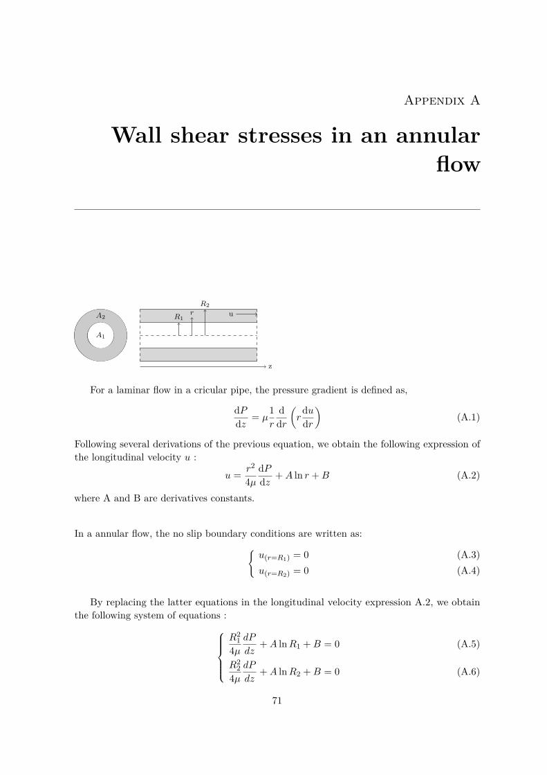
Appendix A

Wall shear stresses in an annularflow

A1

A2

R2r

R1u

z

For a laminar flow in a cricular pipe, the pressure gradient is defined as,

dPdz = µ

1r

ddr

(r

dudr

)(A.1)

Following several derivations of the previous equation, we obtain the following expression ofthe longitudinal velocity u :

u = r2

4µdPdz +A ln r +B (A.2)

where A and B are derivatives constants.

In a annular flow, the no slip boundary conditions are written as:{u(r=R1) = 0 (A.3)u(r=R2) = 0 (A.4)

By replacing the latter equations in the longitudinal velocity expression A.2, we obtainthe following system of equations :

R21

4µdP

dz+A lnR1 +B = 0 (A.5)

R22

4µdP

dz+A lnR2 +B = 0 (A.6)

71

The resolution of this system allows to obtain the expressions of A et B which are :A = 1

4µdPdz

R21 −R2

2ln R2

R1

(A.7)

B = 14µ

dPdz

(−R2

2 −R2

1 −R22

ln R2R1

lnR2

)(A.8)

By replacing the latter equations in the longitudinal velocity expression A.2, the expressionof u becomes :

u = 14µR

22dPdz

((r

R2

)2− 1 + 1− λ2

lnλ ln r

R2

)(A.9)

wherea = R2

2 −R21

ln R2R1

λ = R1R2

Now, we will proceide at defining the mean velocity denoted U . Its expression is,

U = 1Annular section

∫udS = 1

π(R22 −R2

1)

∫ R2

R1u2πrdr

After multiple calculations and a partial integration, the expression of the mean velocity Ubecomes :

U = − 18µR

22dPdz

(1 + λ2 + 1− λ2

lnλ

)

From expressions A.9 et A.9, we deduce the algebraic relation linking the longitudinalvelocity u to the mean velocity U :

u = 2U

1−(rR2

)2− 1−λ2

lnλ ln rR2

1 + λ2 + 1−λ2

lnλ

Finally, let τp1 and τp2 be the wall shear stresses respectively at r = R1 and r = R2. Theirexpressions may be written as :

τp1 = τp(r=R1) = µ

(dudr

)R1

(A.10)

τp2 = τp(r=R2) = µ

(dudr

)R2

(A.11)

In other words, after integrating the expression u, the wall shear stresses τp1 and τp2

72

becomes : τps1 = 2µU

γ

(2R1R2

2+ 1− λ2

R1 lnλ

)(A.12)

τps2 = 2µUγ

(2R2

+ 1− λ2

R2 lnλ

)(A.13)

whereγ = 1 + λ2 + 1− λ2

lnλ

73

Appendix B

Branching conditions

The following subscripts are used : 1 for the interior tube and 2 for the exterior tube.

B.0.0.1 Case 2

•

a

•

b

•

c

•

d

• e

• f

The jump conditions between the points b, c and e are :

(AU)1b = (AU)1c (B.1)

((A2 −A1)U2)b = (AU)2e (B.2)

P1b = P1c

P2b = P2e

P1b = El1b

(A1bA01b

− 1)

+ P2b (B.3)

P1c = El1c

(A1cA01c

− 1)

(B.4)

P2b = El2b

(A2bA02b

− 1)

(B.5)

P2e = El2e

(A2eA02e

− 1)

(B.6)

∫ b

a

∂A1∂t

dx+ (AU)n+11b − (AU)n+1

1a = 0 (B.7)

75

∫ d

c

∂A1∂t

dx+ (AU)n+11d − (AU)n+1

1c = 0 (B.8)

∫ f

e

∂A2∂t

dx+ (AU)n+12f − (AU)n+1

2e = 0 (B.9)

∫ b

a

∂A2∂t

dx+((A2 −A1)U2 +A1U1)n+1

b − ((A2 −A1)U2 +A1U1))n+1

a= 0 (B.10)

Therefore,∆xa2∆ta

(An+1

1a −An1a +An+1

1b −An1b

)+ (AU)n+1

1b − (AU)n+11a = 0 (B.11)

∆xd2∆td

(An+1

1d −An1d +An+1

1c −An1c

)+ (AU)n+1

1d − (AU)n+11c = 0 (B.12)

∆xa2∆ta

(An+1

2a −An2a +An+1

2b −An2b

)+ ((A2 −A1)U2 +A1U1)n+1

b

− ((A2 −A1)U2 +A1U1))n+1a = 0 (B.13)

∆xf2∆tf

(An+1

2f −An2f +An+1

2e −An2e

)+ (AU)n+1

2f − (AU)n+12e = 0 (B.14)

Given that,An+1

2e −An2e = El2b

El2e

A02eA02b

(An+12b −A

n2b) (B.15)

An+11c −A

n1c = El1b

El1c

A01cA01b

(An+11b −A

n1b) + El2b

El1c

A01cA02b

(An+12b −A

n2b) (B.16)

Put,

Ra =( ∆xa

2∆ta

), Rd =

( ∆xd2∆td

), Rf =

(∆xf2∆tf

)

K1bc =El1bEl1c

A01cA01b

, K2be = El2bEl2e

A02eA02b

, K2b1c = El2bEl1c

A01cA02b

By adding (B.11) and (B.12) and using (B.1) and (B.16),

[Ra +RdK1bc](An+11b −A

n1b) +RdK2b1c(An+1

2b −An2b)

= −Ra(An+11a −A

n1a)−Rd(An+1

1d −An1d) + (AU)n+1

1a − (AU)n+11d (B.17)

By substracting equation (B.12) from (B.11),

(AU)n+11b = 1

2(−[Ra −RdK1bc](An+11b −A

n1b) +RdK2b1c(An+1

2b −An2b)

−Ra(An+11a −A

n1a) +Rd(An+1

1d −An1d) + (AU)n+1

1a + (AU)n+11d ) (B.18)

76

By adding (B.13) and (B.14) and using (B.2) and (B.15),

[Ra +RfK2be](An+12b −A

n2b) +Rf (An+1

2f −An2f ) +Ra(An+1

2a −An2a)

+ (AU)n+12f + (AU)n+1

1b − ((A2 −A1)U2 +A1U1))n+1a = 0 (B.19)

By replacing (B.18) in (B.19),

[−Ra2 + RdK1bc2 ](An+1

1b −An1b) + [Ra +RfK2be + RdK2b1c

2 ](An+12b −A

n2b)

= Ra2 (An+1

1a −An1a)−

Rd2 (An+1

1d −An1d)−

(AU)n+11a

2 − (AU)n+11d

2−Rf (An+1

2f −An2f )−Ra(An+1

2a −An2a)− (AU)n+1

2f

+ ((A2 −A1)U2 +A1U1))n+1a (B.20)

Using equations (B.17) and (B.20),(An+1

1b −An1bAn+1

2b −An2b

)= M−1

(Z1Z2

)(B.21)

with,

M =(Ra +RdK1bc RdK2b1c−Ra

2 + RdK1bc2 Ra +RfK2be + RdK2b1c

2

)And,

Z1 = −Ra(An+11a −A

n1a)−Rd(An+1

1d −An1d) + (AU)n+1

1a − (AU)n+11d

Z2 =Ra2 (An+1

1a −An1a)−

Rd2 (An+1

1d −An1d)−

(AU)n+11a

2 − (AU)n+11d

2−Rf (An+1

2f −An2f )−Ra(An+1

2a −An2a)− (AU)n+1

2f

+ ((A2 −A1)U2 +A1U1))n+1a

By susbstracting (B.14) from (B.13), we obtain

[Ra −RfK2be](An+12b −A

n2b) +Ra(An+1

2a −An2a)−Rf (An+1

2f −An2f )

+ 2 (AU)n+12e − (AU)n+1

2f + (AU)n+11b − ((A2 −A1)U2 +A1U1))n+1

a = 0

Therefore,

Un+12e = 1

2An+12e

(−[Ra −RfK2be](An+12b −A

n2b)−Ra(An+1

2a −An2a) (B.22)

+Rf (An+12f −A

n2f ) + (AU)n+1

2f − (AU)n+11b + ((A2 −A1)U2 +A1U1))n+1

a ) (B.23)

From equation (B.21), we obtain An+11b and An+1

2b .

77

From equation (B.3) and (B.5) ,we obtain Pn+11b and Pn+1

2b . Immediately, we obtain Pn+11c and

Pn+12e .

From equation (B.4) and (B.6) ,we obtain An+11c and An+1

2e .From equation (B.11) or (B.18), we obtain Un+1

1b .From equation (B.12) or (B.1), we obtain Un+1

1c .From equation (B.14) or (B.23), we obtain Un+1

2e .From equation (B.13) or(B.2), we obtain Un+1

2b .

B.0.0.2 case 3

•

a

•

b

•

c

•

d

• e

• f

The jump conditions between the points b, c and e are :

(AU)1b = (AU)1c (B.24)

(AU)2e = [(A2 −A1)U2]c (B.25)

P1b = P1c

P2e = P2c

P1b = El1b

(A1bA01b

− 1)

(B.26)

P1c = El1c

(A1cA01c

− 1)

+ P2c (B.27)

P2c = El2c

(A2cA02c

− 1)

(B.28)

P2e = El2e

(A2eA02e

− 1)

(B.29)

Given that, ∫ b

a

∂A1∂t

dx+ (AU)n+11b − (AU)n+1

1a = 0 (B.30)∫ e

f

∂A2∂t

dx+ (AU)n+12e − (AU)n+1

2f = 0 (B.31)

78

∫ d

c

∂A1∂t

dx+ (AU)n+11d − (AU)n+1

1c = 0 (B.32)

∫ d

c

∂A2∂t

dx+((A2 −A1)U2 +A1U1)n+1

d − ((A2 −A1)U2 +A1U1))n+1

c= 0 (B.33)

Therefore,∆xa2∆ta

(An+1

1a −An1a +An+1

1b −An1b

)+ (AU)n+1

1b − (AU)n+11a = 0 (B.34)

∆xf2∆tf

(An+1

2f −An2f +An+1

2e −An2e

)+ (AU)n+1

2e − (AU)n+12f = 0 (B.35)

∆xd2∆td

(An+1

1d −An1d +An+1

1c −An1c

)+ (AU)n+1

1d − (AU)n+11c = 0 (B.36)

∆xd2∆td

(An+1

2d −An2d +An+1

2c −An2c

)+ ((A2 −A1)U2 +A1U1)n+1

d

− ((A2 −A1)U2 +A1U1))n+1c = 0 (B.37)

Given that,An+1

2c −An2c = El2e

El2c

A02cA02e

(An+12e −A

n2e) (B.38)

An+11c −A

n1c = El1b

El1c

A01cA01b

(An+11b −A

n1b)−

El2eEl1c

A01cA02e

(An+12e −A

n2e) (B.39)

Put,

Ra =( ∆xa

2∆ta

), Rd =

( ∆xd2∆td

), Rf =

(∆xf2∆tf

)

K1bc =El1bEl1c

A01cA01b

, K2ec = El2eEl2c

A02cA02e

, K2e1c = El2eEl1c

A01cA02e

By adding (B.34) and (B.36) and using (B.24) and (B.39),

[Ra +RdK1bc](An+11b −A

n1b)−RdK2e1c(An+1

2e −An2e)

= −Ra(An+11a −A

n1a)−Rd(An+1

1d −An1d) + (AU)n+1

1a − (AU)n+11d (B.40)

By substracting equation (B.36) from (B.34),

[Ra −RdK1bc](An+11b −A

n1b) +RdK2e1c(An+1

2e −An2e) +Ra(An+1

1a −An1a)

−Rd(An+11d −A

n1d)− (AU)n+1

1a − (AU)n+11d + 2(AU)n+1

1c ) = 0 (B.41)

79

Therefore,

(AU)n+11c = 1

2(−[Ra −RdK1bc](An+11b −A

n1b)−RdK2e1c(An+1

2e −An2e)

−Ra(An+11a −A

n1a) +Rd(An+1

1d −An1d) + (AU)n+1

1a + (AU)n+11d (B.42)

By adding (B.35) and (B.37) and using (B.25) and (B.38),

[Rf +RdK2ec](An+12e −A

n2e) +Rf (An+1

2f −An2f ) +Rd(An+1

2d −An2d)

− (AU)n+12f − (AU)n+1

1c + ((A2 −A1)U2 +A1U1))n+1d = 0 (B.43)

By replacing (B.42) in (B.43),

[Ra2 −RdK1bc

2 ](An+11b −A

n1b) + [Rf +RdK2ec + RdK2e1c

2 ](An+12e −A

n2e)

= −Ra2 (An+11a −A

n1a) + Rd

2 (An+11d −A

n1d) + (AU)n+1

1a2 + (AU)n+1

1d2

−Rf (An+12f −A

n2f )−Rd(An+1

2d −An2d) + (AU)n+1

2f

− ((A2 −A1)U2 +A1U1))n+1d (B.44)

Using equations (B.40) and (B.44),(An+1

1b −An1bAn+1

2e −An2e

)= M−1

(Z1Z2

)(B.45)

with,

M =(Ra +RdK1bc −RdK2e1cRa2 −

RdK1bc2 Rf +RdK2ec + RdK2e1c

2

)And,

Z1 = −Ra(An+11a −A

n1a)−Rd(An+1

1d −An1d) + (AU)n+1

1a − (AU)n+11d

Z2 =− Ra2 (An+1

1a −An1a) + Rd

2 (An+11d −A

n1d) + (AU)n+1

1a2 + (AU)n+1

1d2

−Rf (An+12f −A

n2f )−Rd(An+1

2d −An2d) + (AU)n+1

2f

− ((A2 −A1)U2 +A1U1))n+1d

By susbstracting (B.37) from (B.35), we obtain

[Rf −RdK2ec](An+12e −A

n2e) +Rf (An+1

2f −An2f )−Rd(An+1

2d −An2d)

− (AU)n+12f − ((A2 −A1)U2 +A1U1))n+1

d + (AU)n+11c + 2 (AU)n+1

2e = 0

80

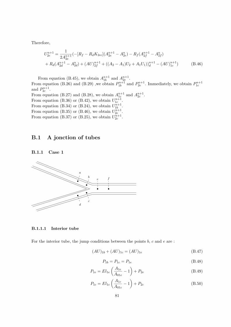
Therefore,

Un+12e = 1

2An+12e

(−[Rf −RdK2ec](An+12e −A

n2e)−Rf (An+1

2f −An2f )

+Rd(An+12d −A

n2d) + (AU)n+1

2f + ((A2 −A1)U2 +A1U1))n+1d − (AU)n+1

1c ) (B.46)

From equation (B.45), we obtain An+11b and An+1

2e .From equation (B.26) and (B.29) ,we obtain Pn+1

1b and Pn+12e . Immediately, we obtain Pn+1

1cand Pn+1

2c .From equation (B.27) and (B.28), we obtain An+1

1c and An+12c .

From equation (B.36) or (B.42), we obtain Un+11c .

From equation (B.34) or (B.24), we obtain Un+11b .

From equation (B.35) or (B.46), we obtain Un+12e .

From equation (B.37) or (B.25), we obtain Un+12c .

B.1 A jonction of tubes

B.1.1 Case 1

•

a

•

b

•

d

•

c

•

e

•

f

B.1.1.1 Interior tube

For the interior tube, the jump conditions between the points b, c and e are :

(AU)1b + (AU)1c = (AU)1e (B.47)

P1b = P1c = P1e (B.48)

P1e = El1e

(A1eA01e

− 1)

+ P2e (B.49)

P1c = El1c

(A1cA01c

− 1)

+ P2c (B.50)

81

P1b = El1b

(A1bA01b

− 1)

+ P2b (B.51)

The conservation of mass equation was derived between a and b, d and c, e and f . We obtain :

∆xf2∆tf

(An+1

1f −An1f +An+1

1e −An1e

)+ (AU)n+1

1f − (AU)n+11e = 0 (B.52)

∆xa2∆ta

(An+1

1a −An1a +An+1

1b −An1b

)+ (AU)n+1

1b − (AU)n+11a = 0 (B.53)

∆xd2∆td

(An+1

1d −An1d +An+1

1c −An1c

)+ (AU)n+1

1c − (AU)n+11d = 0 (B.54)

Given that,An+1

1b −An1b = El1e

El1b

A01bA01e

(An+11e −A

n1e)

An+11c −A

n1c = El1e

El1c

A01cA01e

(An+11e −A

n1e)

Put,

Ra =( ∆xa

2∆ta

), Rd =

( ∆xd2∆td

), Rf =

(∆xf2∆tf

)

K1eb =El1eEl1b

A01bA01e

, K1ec = El1eEl1c

A01cA01e

Adding (B.52), (B.53), (B.54) gives

An+11e =An1e +

(AU)n+11a + (AU)n+1

1d − (AU)n+11f −Ra(A

n+11a −An1a)

Rf +RaK1eb +RdK1ec

−Rd(An+11d −An1d)−Rf (An+1

1f −An1f )Rf +RaK1eb +RdK1ec

(B.55)

Substracting (B.52) from (B.53) and (B.54) gives

Un+11e =

(AU)n+11a + (AU)n+1

1d + (AU)n+11f −Ra(A

n+11a −An1a)−Rd(A

n+11d −An1d)

2An+11e

+Rf (An+11f −An1f ) + (Rf −RaK1eb −RdK1ec)(An+1

1e −An1e)2An+1

1e(B.56)

82

B.1.1.2 Exterior tube

For the exterior tube, the jump conditions between the points b, c and e are :

((A2 −A1)U2)b + ((A2 −A1)U2)c = ((A2 −A1)U2)e (B.57)

P2b = P2c = P2e (B.58)

P2e = El2e

(A2eA02e

− 1)

(B.59)

P2b = El2b

(A2bA02b

− 1)

(B.60)

P2c = El2c

(A2cA02c

− 1)

(B.61)

The conservation of mass equation was derived between a et b, d et c and e et f . We obtain :

∆xa2∆ta

(An+1

2b −An2b +An+1

2a −An2a

)+ ((A2 −A1)U2 +A1U1)n+1

b

− ((A2 −A1)U2 +A1U1)n+1a = 0 (B.62)

∆xd2∆td

(An+1

2d −An2d +An+1

2c −An2c

)+ ((A2 −A1)U2 +A1U1)n+1

c

− ((A2 −A1)U2 +A1U1)n+1d = 0 (B.63)

∆xf2∆tf

(An+1

2f −An2f +An+1

2e −An2e

)+ ((A2 −A1)U2 +A1U1)n+1

f

− ((A2 −A1)U2 +A1U1)n+1e = 0 (B.64)

Put,

∆A =A2 −A1, Ra =( ∆xa

2∆ta

), Rd =

( ∆xd2∆td

)Rf =

(∆xf2∆tf

), K2eb = El2e

El2b

A02bA02e

, K2ec = El2eEl2c

A02cA02e

Adding (B.62), (B.63) and (B.64) gives

An+12e =An2e + (∆AU2 +A1U1)n+1

a + (∆AU2 +A1U1)n+1d

Rf +RaK2eb +RdK2ec

−(∆AU2 +A1U1)n+1f −Ra(An+1

2a −An2a)−Rd(An+12d −An2d)

Rf +RaK2eb +RdK2ec

−Rf (An+12f −An2f )

Rf +RaK2eb +RdK2ec(B.65)

83

Substracting (B.62), (B.63) from (B.64) gives

Un+12e =

(∆AU2 +A1U1)n+1a + (∆AU2 +A1U1)n+1

d + (∆AU2 +A1U1)n+1f

2(A2 −A1)n+1e

+Rf (An+12f −An2f )−Ra(An+1

2a −An2a)−Rd(An+12d −An2d)

2(A2 −A1)n+1e

+(Rf −RaK2eb −RdK2ec)(An+12e −An2e)− 2(AU)n+1

1e2(A2 −A1)n+1

e(B.66)

We notice that the parametres U , P and A of the two tubes are coupled.Therefore, first we could calculate A2e using the equation (B.65).From the equation (B.59), we obtain P2e. Immediately we obtain P2b and P2c.From the equation (B.60) and (B.61), we obtain A2c and A2b.From the equation (B.55), we obtain A1e.From the equation (B.56), we obtain U1e.From the equation (B.49), we obtain P1e. Immediately we obtain P1b and P1c.From the equation (B.50) and (B.51), we obtain A1c and A1b.From the equation (B.53) and (B.54), we obtain U1c and U1b.From the equation (B.66), we obtain U2e.From the equation (B.62) and (B.63), we obtain U2c and U2b.

B.1.2 Case 2

•

a

•

b

•

d

•

c

•

e

•

f

• g

• h

The jump conditions between the points b, c, e and g are :

(AU)1b + (AU)1c = (AU)1e (B.67)

P1b = P1c = P1e (B.68)

84

P1e = El1e

(A1eA01e

− 1)

(B.69)

P1c = El1c

(A1cA01c

− 1)

+ P2c (B.70)

P1b = El1b

(A1bA01b

− 1)

+ P2b (B.71)

((A2 −A1)U2)b + ((A2 −A1)U2)c = (AU)2g (B.72)

P2b = P2c = P2g (B.73)

P2g = El2g

(A2gA02g

− 1)

(B.74)

P2b = El2b

(A2bA02b

− 1)

(B.75)

P2c = El2c

(A2cA02c

− 1)

(B.76)

Giving that,

∆xa2∆ta

(An+1

1a −An1a +An+1

1b −An1b

)+ (AU)n+1

1b − (AU)n+11a = 0 (B.77)

∆xd2∆td

(An+1

1d −An1d +An+1

1c −An1c

)+ (AU)n+1

1c − (AU)n+11d = 0 (B.78)

∆xf2∆tf

(An+1

1f −An1f +An+1

1e −An1e

)+ (AU)n+1

1f − (AU)n+11e = 0 (B.79)

∆xa2∆ta

(An+1

2b −An2b +An+1

2a −An2a

)+ ((A2 −A1)U2 +A1U1)n+1

b

− ((A2 −A1)U2 +A1U1)n+1a = 0 (B.80)

∆xd2∆td

(An+1

2d −An2d +An+1

2c −An2c

)+ ((A2 −A1)U2 +A1U1)n+1

c

− ((A2 −A1)U2 +A1U1)n+1d = 0 (B.81)

∆xh2∆th

(An+1

2h −An2h +An+1

2g −An2g

)+ (AU)n+1

2h − (AU)n+12g = 0 (B.82)

And,An+1

2b −An2b = El2g

El2b

A02bA02g

(An+12g −A

n2g) (B.83)

85

An+12c −A

n2c = El2g

El2c

A02cA02g

(An+12g −A

n2g) (B.84)

An+11c −A

n1c = El1e

El1c

A01cA01e

(An+11e −A

n1e)−

El2gEl1c

A01cA02g

(An+12g −A

n2g) (B.85)

An+11b −A

n1b = El1e

El1b

A01bA01e

(An+11e −A

n1e)−

El2gEl1b

A01bA02g

(An+12g −A

n2g) (B.86)

By adding (B.77), (B.78) and (B.79) and using (B.85) and (B.86),

[Rf +RaK1eb +RdK1ec](An+11e −A

n1e)− (RaK2g1b +RdK2g1c)(An+1

2g −An2g)

= −Ra(An+11a −A

n1a)−Rd(An+1

1d −An1d)−Rf (An+1

1f −An1f ) + (AU)n+1

1a

+ (AU)n+11d − (AU)n+1

1f (B.87)

Writing (B.79)-(B.77)-(B.78) gives,

[Rf −RaK1eb −RdK1ec](An+11e −A

n1e) + (RaK2g1b +RdK2g1c)(An+1

2g −An2g)

−Ra(An+11a −A

n1a)−Rd(An+1

1d −An1d) +Rf (An+1

1f −An1f ) + (AU)n+1

1a

+ (AU)n+11d + (AU)n+1

1f − 2 (AU)n+11e (B.88)

Therefore,

(AU)n+11e =1

2([Rf −RaK1eb −RdK1ec](An+11e −A

n1e)

+ (RaK2g1b +RdK2g1c)(An+12g −A

n2g)−Ra(An+1

1a −An1a)

−Rd(An+11d −A

n1d) +Rf (An+1

1f −An1f ) + (AU)n+1

1a

+ (AU)n+11d + (AU)n+1

1f ) (B.89)

Writing (B.80), (B.81) and (B.82) and using (B.83) and (B.84),

[Rh +RaK2gb +RdK2gc](An+12g −A

n2g) +Rh(An+1

2h −An2h) +Ra(An+1

2a −An2a)

+Rd(An+12d −A

n2d) + (AU)n+1

1e − ((A2 −A1)U2 +A1U1)n+1a

− ((A2 −A1)U2 +A1U1)n+1d + (AU)n+1

2h = 0 (B.90)

86

By replacing (B.89) in (B.90),

[Rf2 −RaK1eb

2 − RdK1ec2 ](An+1

1e −An1e)

+ (RaK2g1b2 + RdK2g1c

2 +Rh +RaK2gb +RdK2gc)(An+12g −A

n2g)

= Ra2 (An+1

1a −An1a) + Rd

2 (An+11d −A

n1d)−

Rf2 (An+1

1f −An1f ) (B.91)

− (AU)n+11a

2 − (AU)n+11d

2 −(AU)n+1

1f2 −Rh(An+1

2h −An2h)−Ra(An+1

2a −An2a)

−Rd(An+12d −A

n2d) + ((A2 −A1)U2 +A1U1)n+1

a + ((A2 −A1)U2 +A1U1)n+1d

− (AU)n+12h (B.92)

Using equations (B.87) and (B.92)(An+1

1e −An1eAn+1

2g −An2g

)= M−1

(Z1Z2

)(B.93)

with,

M =(Rf +RaK1eb +RdK1ec −RaK2g1b −RdK2g1cRf

2 −RaK1eb

2 − RdK1ec2

RaK2g1b

2 + RdK2g1c

2 +Rh +RaK2gb +RdK2gc

)

And,

Z1 =−Ra(An+11a −A

n1a)−Rd(An+1

1d −An1d)−Rf (An+1

1f −An1f ) + (AU)n+1

1a

+ (AU)n+11d − (AU)n+1

1f

Z2 =Ra2 (An+1

1a −An1a) + Rd

2 (An+11d −A

n1d)−

Rf2 (An+1

1f −An1f )

− (AU)n+11a

2 − (AU)n+11d

2 −(AU)n+1

1f2 −Rh(An+1

2h −An2h)

−Ra(An+12a −A

n2a)−Rd(An+1

2d −An2d) + ((A2 −A1)U2 +A1U1)n+1

a

+ ((A2 −A1)U2 +A1U1)n+1d − (AU)n+1

2h

(B.82)-(B.80)-(B.81)

[Rh −RaK2gb −RdK2gc](An+12g −A

n2g)− (AU)n+1

1e + (AU)n+12h

+ ((A2 −A1)U2 +A1U1)n+1a + ((A2 −A1)U2 +A1U1)n+1

d − 2 (AU)n+12g = 0

87

Therefore,

Un+12g = 1

2An+12g

([Rh −RaK2gb −RdK2gc](An+12g −A

n2g)− (AU)n+1

1e + (AU)n+12h

+ ((A2 −A1)U2 +A1U1)n+1a + ((A2 −A1)U2 +A1U1)n+1

d ) (B.94)

where

Ra =( ∆xa

2∆ta

), Rd =

( ∆xd2∆td

), Rf =

(∆xf2∆tf

)

Rh =( ∆xh

2∆th

), K1eb = El1b

El1e

A01eA01b

, K1ec = El1cEl1e

A01eA01c

K2gb =El2gEl2b

A02bA02g

, K2gc = El2gEl2c

A02cA02g

, K2g1b = El2gEl1b

A01bA02g

K2g1c =El2gEl1c

A01cA02g

From equation (B.93), we obtain An+11e and An+1

2g .From equation (B.69) and (B.74) ,we obtain Pn+1

1e and Pn+12g . Immediately, we obtain Pn+1

1b ,Pn+1

1c , Pn+12b , Pn+1

2c .From equation (B.70), (B.71), (B.75) and (B.76) ,we obtain An+1

1b , An+11c , An+1

2b , An+12c .

From equation (B.89) or (B.79), we obtain Un+11e .

From equation (B.77) and (B.78) we obtain Un+11b and Un+1

1c .From equation (B.94) or (B.82), we obtain Un+1

2g .From equation (B.80) and (B.81) we obtain Un+1

2b and Un+12c .

B.1.3 Case 3

•

a

•

b

•

d

•

c

•

e

•

f

• g

• h

The jump conditions between the points b, c, e and g are :

88

(AU)1b + (AU)1c = (AU)1e (B.95)

P1b = P1c = P1e (B.96)

P1e = El1e

(A1eA01e

− 1)

(B.97)

P1c = El1c

(A1cA01c

− 1)

(B.98)

P1b = El1b

(A1bA01b

− 1)

+ P2b (B.99)

((A2 −A1)U2)b = (AU)2g (B.100)

P2b = P2g (B.101)

P2g = El2g

(A2gA02g

− 1)

(B.102)

P2b = El2b

(A2bA02b

− 1)

(B.103)

Given that,

∆xa2∆ta

(An+1

1a −An1a +An+1

1b −An1b

)+ (AU)n+1

1b − (AU)n+11a = 0 (B.104)

∆xd2∆td

(An+1

1d −An1d +An+1

1c −An1c

)+ (AU)n+1

1c − (AU)n+11d = 0 (B.105)

∆xf2∆tf

(An+1

1f −An1f +An+1

1e −An1e

)+ (AU)n+1

1f − (AU)n+11e = 0 (B.106)

∆xa2∆ta

(An+1

2b −An2b +An+1

2a −An2a

)+ ((A2 −A1)U2 +A1U1)n+1

b

− ((A2 −A1)U2 +A1U1)n+1a = 0 (B.107)

∆xh2∆th

(An+1

2h −An2h +An+1

2g −An2g

)+ (AU)n+1

2h − (AU)n+12g = 0 (B.108)

And,An+1

2b −An2b = El2g

El2b

A02bA02g

(An+12g −A

n2g) (B.109)

An+11c −A

n1c = El1e

El1c

A01cA01e

(An+11e −A

n1e) (B.110)

89

An+11b −A

n1b = El1e

El1b

A01bA01e

(An+11e −A

n1e)−

El2gEl1b

A01bA02g

(An+12g −A

n2g) (B.111)

Put,

Ra =( ∆xa

2∆ta

)Rd =

( ∆xd2∆td

)Rf =

(∆xf2∆tf

)

Rh =( ∆xh

2∆th

)K1eb = El1e

El1b

A01bA01e

K1ec = El1eEl1c

A01cA01e

K2gb =El2gEl2b

A02bA02g

K2g1b = El2gEl1b

A01bA02g

By adding (B.104), (B.105) and (B.106) and using (B.110) and (B.111),

[Rf +RaK1eb +RdK1ec](An+11e −A

n1e)−RaK2g1b(An+1

2g −An2g)

= −Ra(An+11a −A

n1a)−Rd(An+1

1d −An1d)−Rf (An+1

1f −An1f ) + (AU)n+1

1a

+ (AU)n+11d − (AU)n+1

1f (B.112)

Writing (B.106)+(B.105)-(B.104) gives,

[Rf −RaK1eb +RdK1ec](An+11e −A

n1e) +RaK2g1b(An+1

2g −An2g)−Ra(An+1

1a −An1a)

+Rd(An+11d −A

n1d) +Rf (An+1

1f −An1f ) + (AU)n+1

1f − (AU)n+11d + (AU)n+1

1a

− 2 (AU)n+11b = 0 (B.113)

Therefore,

(AU)n+11b =1

2([Rf −RaK1eb +RdK1ec](An+11e −A

n1e) +RaK2g1b(An+1

2g −An2g)

−Ra(An+11a −A

n1a) +Rd(An+1

1d −An1d) +Rf (An+1

1f −An1f )

+ (AU)n+11f − (AU)n+1

1d + (AU)n+11a ) (B.114)

By adding (B.107) and (B.108) and using (B.109) and (B.84),

[Rh +RaK2gb](An+12g −A

n2g) +Rh(An+1

2h −An2h) +Ra(An+1

2a −An2a)

+ (AU)n+11b − ((A2 −A1)U2 +A1U1)n+1

a + (AU)n+12h = 0 (B.115)

90

By replacing (B.114) in (B.115),

[Rf2 −RaK1eb

2 + RdK1ec2 ](An+1

1e −An1e)

+ [RaK2g1b2 +Rh +RaK2gb](An+1

2g −An2g)

= (AU)n+11d

2 − (AU)n+11a

2 −(AU)n+1

1f2 + Ra

2 (An+11a −A

n1a)−

Rd2 (An+1

1d −An1d)

− Rf2 (An+1

1f −An1f )−Rh(An+1

2h −An2h)−Ra(An+1

2a −An2a)

+ ((A2 −A1)U2 +A1U1)n+1a − (AU)n+1

2h (B.116)

Using equations (B.112) and (B.92)(An+1

1e −An1eAn+1

2g −An2g

)= M−1

(Z1Z2

)(B.117)

with,

M =(Rf +RaK1eb +RdK1ec −RaK2g1bRf

2 −RaK1eb

2 + RdK1ec2

RaK2g1b

2 +Rh +RaK2gb

)And,

Z1 =−Ra(An+11a −A

n1a)−Rd(An+1

1d −An1d)−Rf (An+1

1f −An1f ) + (AU)n+1

1a

+ (AU)n+11d − (AU)n+1

1f

Z2 =(AU)n+11d

2 − (AU)n+11a

2 −(AU)n+1

1f2 + Ra

2 (An+11a −A

n1a)−

Rd2 (An+1

1d −An1d)

− Rf2 (An+1

1f −An1f )−Rh(An+1

2h −An2h)−Ra(An+1

2a −An2a)

+ ((A2 −A1)U2 +A1U1)n+1a − (AU)n+1

2h

Writing (B.108)-(B.107) gives,

[Rh −RaK2gb](An+12g −A

n2g) +Rh(An+1

2h −An2h)−Ra(An+1

2a −An2a)

+ (AU)n+12h − 2(AU)n+1

2g − (AU)n+11b + ((A2 −A1)U2 +A1U1)n+1

a = 0 (B.118)

Therefore,

Un+12g = 1

2An+12g

([Rh −RaK2gb](An+12g −A

n2g) +Rh(An+1

2h −An2h)

−Ra(An+12a −A

n2a) + (AU)n+1

2h − (AU)n+11b

+ ((A2 −A1)U2 +A1U1)n+1a ) (B.119)

91

From equation (B.117), we obtain An+11e and An+1

2g .From equation (B.97) and (B.102) ,we obtain Pn+1

1e and Pn+12g . Immediately, we obtain Pn+1

1b ,Pn+1

1c and Pn+12b .

From equation (B.98), (B.99) and (B.103), we obtain An+11c , An+1

1b and An+12b .

From equation (B.104) or (B.114), we obtain Un+11b .

From equation (B.105) and (B.106) we obtain Un+11c and Un+1

1e .From equation (B.119) or (B.108), we obtain Un+1

2g .From equation (B.100) or (B.107) we obtain Un+1

2b .

B.2 A Bifurcation of tubes

B.2.1 Case 1

•

e

•

f

•

b

•

a

•

c

•

d

B.2.1.1 Interior tube

For the interior tube, the jump conditions between the points b, c and e are :

(AU)1b + (AU)1c = (AU)1e (B.120)

P1b = P1c = P1e (B.121)

P1e = El1e

(A1eA01e

− 1)

+ P2e (B.122)

P1c = El1c

(A1cA01c

− 1)

+ P2c (B.123)

P1b = El1b

(A1bA01b

− 1)

+ P2b (B.124)

The conservation of mass equation was derived between a et b, d et c and e et f . We obtain :

∆xf2∆tf

(An+1

1f −An1f +An+1

1e −An1e

)+ (AU)n+1

1e − (AU)n+11f = 0 (B.125)

92

∆xa2∆ta

(An+1

1a −An1a +An+1

1b −An1b

)+ (AU)n+1

1a − (AU)n+11b = 0 (B.126)

∆xd2∆td

(An+1

1d −An1d +An+1

1c −An1c

)+ (AU)n+1

1d − (AU)n+11c = 0 (B.127)

Giving that,An+1

1b −An1b = El1e

El1b

A01bA01e

(An+11e −A

n1e)

An+11c −A

n1c = El1e

El1c

A01cA01e

(An+11e −A

n1e)

Put,

Ra =( ∆xa

2∆ta

), Rd =

( ∆xd2∆td

), Rf =

(∆xf2∆tf

)

K1eb =El1eEl1b

A01bA01e

, K1ec = El1eEl1c

A01cA01e

Adding (B.125), (B.126) and (B.127) gives,

An+11e =An1e +

(AU)n+11f − (AU)n+1

1a − (AU)n+11d −Ra(A

n+11a −An1a)

Rf +RaK1eb +RdK1ec

−Rd(An+11d −An1d)−Rf (An+1

1f −An1f )Rf +RaK1eb +RdK1ec

(B.128)

Substracting (B.125) and (B.126) from (B.127) gives,

Un+11e =

(AU)n+11a + (AU)n+1

1d + (AU)n+11f +Ra(An+1

1a −An1a) +Rd(An+11d −An1d)

2An+11e

−Rf (An+11f −An1f )− (Rf −RaK1eb −RdK1ec)(An+1

1e −An1e)2An+1

1e(B.129)

B.2.1.2 Exterior tube

For the exterior tube, the jump conditions between the points b, c and e are :

((A2 −A1)U2)b + ((A2 −A1)U2)c = ((A2 −A1)U2)e (B.130)

P2b = P2c = P2e (B.131)

P2e = El2e

(A2eA02e

− 1)

(B.132)

93

P2b = El2b

(A2bA02b

− 1)

(B.133)

P2c = El2c

(A2cA02c

− 1)

(B.134)

The conservation of mass equation was derived between a et b, d et c and e et f . We obtain :

∆xa2∆ta

(An+1

2b −An2b +An+1

2a −An2a

)+ ((A2 −A1)U2 +A1U1)n+1

a

− ((A2 −A1)U2 +A1U1)n+1b = 0 (B.135)

∆xd2∆td

(An+1

2d −An2d +An+1

2c −An2c

)+ ((A2 −A1)U2 +A1U1)n+1

d

− ((A2 −A1)U2 +A1U1)n+1c = 0 (B.136)

∆xf2∆tf

(An+1

2f −An2f +An+1

2e −An2e

)+ ((A2 −A1)U2 +A1U1)n+1

e

− ((A2 −A1)U2 +A1U1)n+1f = 0 (B.137)

Put,

∆A =A2 −A1, Ra =( ∆xa

2∆ta

), Rd =

( ∆xd2∆td

)Rf =

(∆xf2∆tf

), K2eb = El2e

El2b

A02bA02e

, K2ec = El2eEl2c

A02cA02e

Adding (B.135), (B.136) and (B.137) gives, :

An+12e =An2e +

(∆AU2 +A1U1)n+1f − (∆AU2 +A1U1)n+1

a

Rf +RaK2eb +RdK2ec

−(∆AU2 +A1U1)n+1d −Ra(An+1

2a −An2a)−Rd(An+12d −An2d)

Rf +RaK2eb +RdK2ec

−Rf (An+12f −An2f )

Rf +RaK2eb +RdK2ec(B.138)

94

Substracting (B.135) and (B.136) from (B.137) gives,

Un+12e =

(∆AU2 +A1U1)n+1a + (∆AU2 +A1U1)n+1

d + (∆AU2 +A1U1)n+1f

2(A2 −A1)n+1e

−Rf (An+12f −An2f ) +Ra(An+1

2a −An2a) +Rd(An+12d −An2d)

2(A2 −A1)n+1e

−(Rf −RaK2eb −RdK2ec)(An+12e −An2e)− 2(AU)n+1

1e2(A2 −A1)n+1

e(B.139)

We notice that the parametres U , P and A of the two tubes are coupled.Therefore, first we could calculate A2e using the equation (B.138).From the equation (B.132), we obtain P2e. Immediately we obtain P2b and P2c.From the equation (B.133) and (B.134), we obtain A2c and A2b.From the equation (B.128), we obtain A1e.From the equation (B.129), we obtain U1e.From the equation (B.122), we obtain P1e. Immediately we obtain P1b and P1c.From the equation (B.123) and (B.124), we obtain A1c and A1b.From the equation (B.126) and (B.127), we obtain U1c and U1b.From the equation (B.139), we obtain U2e.From the equation (B.135) and (B.136), we obtain U2c and U2b.

B.2.2 Case 2

•

e

•

f

•

b

•

a

•

c

•

d

•g

•h

The jump conditions between the points b, c, e and g are :

(AU)1b + (AU)1c = (AU)1e (B.140)

P1b = P1c = P1e (B.141)

95

P1e = El1e

(A1eA01e

− 1)

+ P2e (B.142)

P1c = El1c

(A1cA01c

− 1)

(B.143)

P1b = El1b

(A1bA01b

− 1)

+ P2b (B.144)

((A2 −A1)U2)b + (AU)2g = ((A2 −A1)U2)e (B.145)

P2b = P2e = P2g (B.146)

P2g = El2g

(A2gA02g

− 1)

(B.147)

P2b = El2b

(A2bA02b

− 1)

(B.148)

P2e = El2e

(A2eA02e

− 1)

(B.149)

Giving that,

∆xa2∆ta

(An+1

1a −An1a +An+1

1b −An1b

)+ (AU)n+1

1a − (AU)n+11b = 0 (B.150)

∆xd2∆td

(An+1

1d −An1d +An+1

1c −An1c

)+ (AU)n+1

1d − (AU)n+11c = 0 (B.151)

∆xf2∆tf

(An+1

1f −An1f +An+1

1e −An1e

)+ (AU)n+1

1e − (AU)n+11f = 0 (B.152)

∆xa2∆ta

(An+1

2b −An2b +An+1

2a −An2a

)+ ((A2 −A1)U2 +A1U1)n+1

a

− ((A2 −A1)U2 +A1U1)n+1b = 0 (B.153)

∆xf2∆tf

(An+1

2e −An2e +An+1

2f −An2f

)+ ((A2 −A1)U2 +A1U1)n+1

e

− ((A2 −A1)U2 +A1U1)n+1f = 0 (B.154)

∆xh2∆th

(An+1

2h −An2h +An+1

2g −An2g

)+ (AU)n+1

2h − (AU)n+12g = 0 (B.155)

And,An+1

2b −An2b = El2g

El2b

A02bA02g

(An+12g −A

n2g) (B.156)

96

An+12e −A

n2e = El2g

El2e

A02eA02g

(An+12g −A

n2g) (B.157)

An+11c −A

n1c = El1e

El1c

A01cA01e

(An+11e −A

n1e) + El2g

El1c

A01cA02g

(An+12g −A

n2g) (B.158)

An+11b −A

n1b = El1e

El1b

A01bA01e

(An+11e −A

n1e) (B.159)

By adding (B.150), (B.151) and (B.152) and using (B.140), (B.158) and (B.159),

[Rf +RaK1eb +RdK1ec](An+11e −A

n1e) +RdK2g1c(An+1

2g −An2g)

= −Ra(An+11a −A

n1a)−Rd(An+1

1d −An1d)−Rf (An+1

1f −An1f )− (AU)n+1

1a

− (AU)n+11d + (AU)n+1

1f (B.160)

Writing (B.150)+(B.152)-(B.151) gives,

[Rf +RaK1eb −RdK1ec](An+11e −A

n1e)−RdK2g1c(An+1

2g −An2g)

+Ra(An+11a −A

n1a)−Rd(An+1

1d −An1d) +Rf (An+1

1f −An1f ) + (AU)n+1

1a

− (AU)n+11d − (AU)n+1

1f + 2 (AU)n+11c (B.161)

Therefore,

(AU)n+11c =1

2(−[Rf +RaK1eb −RdK1ec](An+11e −A

n1e) +RdK2g1c(An+1

2g −An2g)

−Ra(An+11a −A

n1a) +Rd(An+1

1d −An1d)−Rf (An+1

1f −An1f )

− (AU)n+11a + (AU)n+1

1d + (AU)n+11f ) (B.162)

By adding (B.153), (B.154) and (B.155) and using (B.156), (B.157), (B.140) and (B.145),

[Rh +RaK2gb +RfK2ge](An+12g −A

n2g) +Ra(An+1

2a −An2a) +Rf (An+1

2f −An2f )

+Rh(An+12h −A

n2h) + ((A2 −A1)U2 +A1U1)n+1

a − ((A2 −A1)U2 +A1U1)n+1f

+ (AU)n+12h + (AU)n+1

1c = 0 (B.163)

97

By replacing (B.162) in (B.163)

(−Rf2 −RaK1eb

2 + RdK1ec2 ](An+1

1e −An1e)

+ [RdK21gc2 +Rh +RaK2gb +RfK2ge](An+1

2g −An2g) =

Ra2 (An+1

1a −An1a)−

Rd2 (An+1

1d −An1d) + Rf

2 (An+11f −A

n1f ) + (AU)n+1

1a2

− (AU)n+11d

2 −(AU)n+1

1f2 −Ra(An+1

2a −An2a)−Rf (An+1

2f −An2f )

−Rh(An+12h −A

n2h)− ((A2 −A1)U2 +A1U1)n+1

a + ((A2 −A1)U2 +A1U1)n+1f

− (AU)n+12h (B.164)

Using equations (B.160) and (B.164)(An+1

1e −An1eAn+1

2g −An2g

)= M−1

(Z1Z2

)(B.165)

with,

M =(Rf +RaK1eb +RdK1ec RdK2g1c

−Rf

2 −RaK1eb

2 + RdK1ec2

RdK2g1c

2 +Rh +RaK2gb +RfK2ge

)

And,

Z1 =−Ra(An+11a −A

n1a)−Rd(An+1

1d −An1d)−Rf (An+1

1f −An1f )− (AU)n+1

1a

− (AU)n+11d + (AU)n+1

1f

Z2 =Ra2 (An+1

1a −An1a)−

Rd2 (An+1

1d −An1d) + Rf

2 (An+11f −A

n1f ) + (AU)n+1

1a2

− (AU)n+11d

2 −(AU)n+1

1f2 −Ra(An+1

2a −An2a)−Rf (An+1

2f −An2f )

−Rh(An+12h −A

n2h)− ((A2 −A1)U2 +A1U1)n+1

a

+ ((A2 −A1)U2 +A1U1)n+1f − (AU)n+1

2h

Writing (B.154)+(B.153)-(B.155) gives,

[−Rh +RaK2gb +RfK2ge](An+12g −A

n2g) +Ra(An+1

2a −An2a)

+Rf (An+12f −A

n2f )−Rh(An+1

2h −An2h) + ((A2 −A1)U2 +A1U1)n+1

a

− ((A2 −A1)U2 +A1U1)n+1f − (AU)n+1

2h + 2(AU)n+12g + (AU)n+1

1c

= 0

98

Therefore,

Un+12g = 1

2An+12g

([Rh −RaK2gb −RfK2ge](An+12g −A

n2g)−Ra(An+1

2a −An2a)

−Rf (An+12f −A

n2f ) +Rh(An+1

2h −An2h)− ((A2 −A1)U2 +A1U1)n+1

a

+ ((A2 −A1)U2 +A1U1)n+1f + (AU)n+1

2h − (AU)n+11c ) (B.166)

From equation (B.165), we obtain An+11e and An+1

2g .From equation (B.142) and (B.147) ,we obtain Pn+1

1e and Pn+12g . Immediately, we obtain Pn+1

1b ,Pn+1

1c , Pn+12b , Pn+1

2e .From equation (B.143), (B.144), (B.148) and (B.149), we obtain An+1

1c , An+11b , An+1

2b and An+12e .

From equation (B.162) or (B.151), we obtain Un+11c .

From equation (B.150) and (B.152) we obtain Un+11b and Un+1

1e .From equation (B.166) or (B.155), we obtain Un+1

2g .From equation (B.153) and (B.154) we obtain Un+1

2b and Un+12e .

99

Appendix C

A one dimensional model of theCerebrospinal Fluid Flow in thespinal canal: study of the fluid

viscosity and the steady/unsteadyflow effects

The following article has been submited to the Physics of Fluids journal and is currentlyundergoing reviews.

101

A one dimensional model of the Cerebrospinal FluidFlow in the spinal canal: study of the fluid viscosity

and the steady/unsteady flow effects

Maher M., Cathalifaud P., Zagzoule M.

Institut de Mecanique des Fluides de Toulouse (IMFT), Universite de Toulouse, CNRS,INPT, UPS, Toulouse, France

Abstract

In this study, a one dimensional-model (1-D) for the flow in elastic pipes is used

to simulate the dynamics of the Cerebrospinal Fluid (CSF) in the spinal canal.

The modelling is based around two coaxial tubes filled with CSF. The inner

tube represents the Spinal Cord (SC) and the outer one represents the Spinal

Subarachnoid Space (SSS). The conservation of mass and momentum in 1D is

applied to the two coupled tubes. The modelling accounts for the viscosity of

the CSF. Specific attention is given to the effect of the CSF viscosity on the

wave propagtion modes. Moreover, this work confronts the wall shear stress of

a quasi-steady flow approximation used in 1-D modelling against the wall shear

stress for an unsteady flow in an annuli.

Keywords: Spinal canal, coaxial tubes, 1D model, Cerebropsinal Fluid,

conicity, viscosity

1. Introduction

The Cerebrospinal fluid (CSF) is a fluid close to water which is mainly contained

in cavities in the brain called ventricles and anatomic spaces called cranial and

spinal subarachnoid spaces (SSS). The SSS is an annular space surrounding the

spinal cord (SC). Three protective membranes, called the meninges lies within5

Preprint submitted to Journal of Physics of Fluids May 13, 2019102

the spinal cord. The pia-matter adheres to the surface of the spinal cord. The

dura-matter and the arachnoid-matter envelop the SSS.

The CSF circulation depends on the arterial pulse wave and displays a pulsat-

ing motion between the cranial and the spinal compartment. Additional factors

such as the respiratory waves and the subject’s posture also modulates the CSF10

dynamics (Haughton and Mardal, 2014; Sakka et al., 2011).

CSF velocity wave in the spinal canal is of interest as a potential indicator

of CSF system pressure and compliance. It is considered an important fac-

tor influencing the pathogenesis of craniospinal disorder such as hydrocephalus,

chiari malformation and syringomyelia (Luciano and Dombrowski, 2007; Flana-15

gan, 2015). Several analytical (Lockey et al., 1975; Cirovic, 2009; Cirovic and

Kim, 2012; Elliott et al., 2017; Berkouk et al., 2003; Carpenter et al., 2003)

and computational studies (Bertram, 2009; Bertram et al., 2005) have used the

idealised geometry of coaxial and compliant tubes to understand the dynamics

of the CSF in the spinal canal. Based on MRI flow measurements in a healthy20

volunteer, Loth et al. (2001) computed a linearized Navier-Stokes model of the

CSF flow in the spinal subarachnoid space (SSS). It has been observed that the

Womersley number ranged from 5 to 17. It relates flow pulsatility (unsteady or

inertial forces) to fluid viscosity (viscous forces), and is used to characterize flow

dynamics. For normal physiological flow rates and CSF fluid properties, results25

have shown that for large annular gaps, inertial effects tend to dominate the flow

field and for small annular gaps, viscous effect dominate the flow. Reduction

of the SSS radius occur in CSF related disorders. For example in Chiari mal-

formations where the cerebellar tonsils herniates into the cervical spinal canal

or in syringomyelia where spinal cord swells. This reduction will change the30

hydrodynamic system from interia dominated to mixed (inertia+viscous) an in

extreme cases, to a viscous dominated flow. Since then in posterior studies,

to the best of our knowledge, the CSF viscosity is usually being neglected in

1-D modelling of the flow in the spinal canal. In this study, we developp a

one-dimensionnal (1-D) modelling of the spinal canal as coaxial and compliant35

tubes with particular attention to the viscosity of the CSF in the SSS.

2103

Furthermore, when accounting for the CSF viscosity, in order to solve the 1-D

governing equation, one must make an assumption on the local velocity profile

or the unsteady nature of the flow for a proper estimation of the wall shear40

stresses in both circular and annular section. The Womersley number gives a

strong indication on the profile. In general, for Wo < 1, in a circular tube the

fluid velocity profile is parabolic and the flow rate is in phase with the pressure

gradient. The fluid profile loses its parabolic shape when Wo > 1, and a phase

lag between pressure and flow rate becomes more pronounced as the Womersley45

number reaches ten or more (Womersley, 1955).

The present work first presents the 1-D geometry and governing equations for a

viscous CSF. The wall shear stresses in the coaxial geometry are evaluated on

the assumption of a quasi-steady flow state. Next, wave propagation modes are50

characterized. An analytical solution of the wave equation is proposed for an

inviscid CSF flow and for a viscous one. Finally, using the work of Tsangaris

(1984), an analytical solution of the wall shear stresses in annular section of a

viscous flow due ton an oscillating pressure is presented. The limitations of the

quasi-steady flow assumption in an annular section is discussed. Accordingly,55

the theoretical study of an unsteady flow in a circular annuli can be viewed as

fundamental and independent of the particular application to the spinal CSF

system.

2. Geometry and approximations60

The idealized geometry around which the theory is based is illustrated in Figure

1. It consists of two coaxial and elastic tubes. The inner tube represents the

SC which is envelopped by the pia-matter. The outer tube represents the SSS

and is filled with CSF. The dura-matter envelops the SSS.

3104

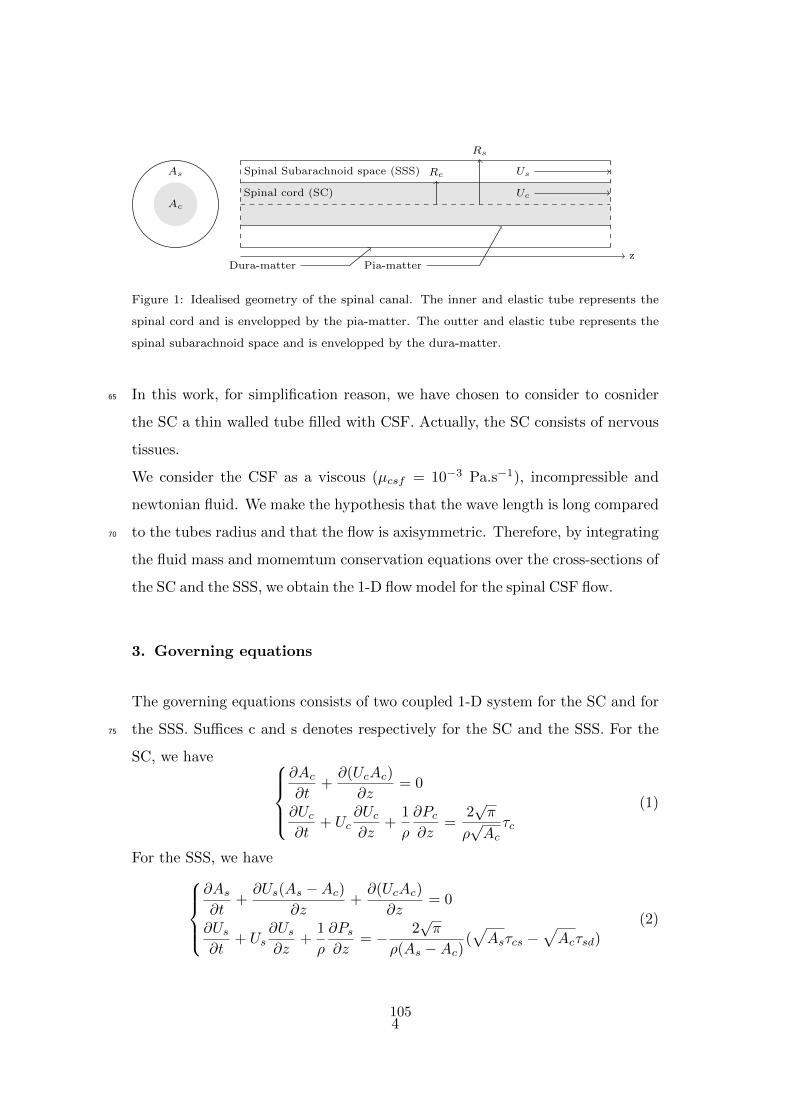
Ac

As

Spinal cord (SC)

Spinal Subarachnoid space (SSS) Us

Uc

zDura-matter Pia-matter

Rs

Rc

Figure 1: Idealised geometry of the spinal canal. The inner and elastic tube represents the

spinal cord and is envelopped by the pia-matter. The outter and elastic tube represents the

spinal subarachnoid space and is envelopped by the dura-matter.

In this work, for simplification reason, we have chosen to consider to cosnider65

the SC a thin walled tube filled with CSF. Actually, the SC consists of nervous

tissues.

We consider the CSF as a viscous (µcsf = 10−3 Pa.s−1), incompressible and

newtonian fluid. We make the hypothesis that the wave length is long compared

to the tubes radius and that the flow is axisymmetric. Therefore, by integrating70

the fluid mass and momemtum conservation equations over the cross-sections of

the SC and the SSS, we obtain the 1-D flow model for the spinal CSF flow.

3. Governing equations

The governing equations consists of two coupled 1-D system for the SC and for

the SSS. Suffices c and s denotes respectively for the SC and the SSS. For the75

SC, we have

∂Ac∂t

+∂(UcAc)

∂z= 0

∂Uc∂t

+ Uc∂Uc∂z

+1

ρ

∂Pc∂z

=2√π

ρ√Acτc

(1)

For the SSS, we have

∂As∂t

+∂Us(As −Ac)

∂z+∂(UcAc)

∂z= 0

∂Us∂t

+ Us∂Us∂z

+1

ρ

∂Ps∂z

= − 2√π

ρ(As −Ac)(√Asτcs −

√Acτsd)

(2)

4105

where z and t are respectively axial coordinate and time, A is the cross-sectional

area, U and P are the axial velocity and pressure of the CSF respectively av-

eraged over the cross sectional area, τc is the wall shear stress at (r = Rc) due

to the friction between the CSF in the SC and the pia-matter, τcs is the wall

shear stress at (r = Rc) due to the friction between the CSF in the SSS and the

pia-matter and τsd the wall shear stress at (r = Rs) due to the friction between

the CSF in the SSS and the dura-matter.

The wall shear stresses τc, τcs and τsd are expressed as

τc = µ

(∂uc∂r

)

r=Rc

τcs = µ

(∂us∂r

)

r=Rc

τsd = µ

(∂us∂r

)

r=Rs

At this point to solve the system of the coupled equations, we need to make an

assumption on the local velocity profile in order to obtain an estimation of the

above wall shear stresses. For a simplification matter, we assume a quasi-steady

flow approximation. ”Quasi steady” does not mean ”approximately steady” (i.e,

not changing very much in time). Rather ”Quasi steady” means that at any

time the instantaneous fow rate is determined by the instantaneous pressure

gradient. In the last section of this paper, we will discuss the validity of this

hypothesis in the SSS.

For the SC, this assumption leads to the commonly known Hagen-Poiseuille flow

whose velocity profile is

uc = 2Uc

(1−

(r

Rc0

)2)

According to (3), the wall shear stress, τc, is thus given by

τc = −4µUcRc0

For the SSS, giving the pressure gradient for a laminar steady flow in a straight

rigid tube∂ps∂z

= µ1

r

∂

∂r

(r∂us∂r

)

5106

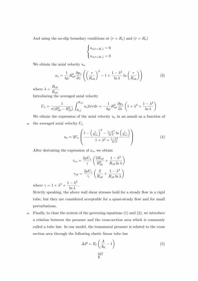
And using the no-slip boundary conditions at (r = Rc) and (r = Rs)

us(r=Rc) = 0

us(r=Rs) = 0

We obtain the axial velocity us

us =1

4µR2s0

∂ps∂z

((r

Rs0

)2

− 1 +1− λ2

lnλln

(r

Rs0

))(3)

where λ =Rc0Rs0

.

Introducing the averaged axial velocity

Us =1

π(R2s0 −R2

c0)

∫ Rs0

Rc0

us2πrdr = − 1

8µR2s0

∂ps∂z

(1 + λ2 +

1− λ2lnλ

)

We obtain the expression of the axial velocity us in an annuli as a function of

the averaged axial velocity Us80

us = 2Us

1−(

rRs0

)2− 1−λ2

lnλ ln(

rRs0

)

1 + λ2 + 1−λ2

lnλ

(4)

After derivating the expression of us, we obtain

τcs =2µUsγ

(2Rc0R2s0

+1− λ2Rc0 lnλ

)

τsd =2µUsγ

(2

Rs0+

1− λ2Rs0 lnλ

)

where γ = 1 + λ2 +1− λ2

lnλ.

Strictly speaking, the above wall shear stresses hold for a steady flow in a rigid

tube, but they are considered acceptable for a quasi-steady flow and for small

perturbations.

Finally, to close the system of the governing equations (1) and (2), we introduce85

a relation between the pressure and the cross-section area which is commonly

called a tube law. In our model, the transmural pressure is related to the cross

section area through the following elastic linear tube law

∆P = El

(A

A0− 1

)(5)

6107

where ∆P is the transmural pressure, El is the elastance of the tube and de-

notes its mechanical properties, A0 is the cross-section area at zero transmural90

pressure. Using this tube law for the SC and SSS tubes and assuming a constant

pressure surrounding the dura-matter, we obtain

∆P = Pc − Ps = Elc

(AcA0c− 1

)

Ps = Els

(AsA0s− 1

) (6)

where Elc is the elastance of the pia-matter and Els is the elastance of the

dura-matter. Elc and Els are assumed constant.

The solution of the coupled system (1), (2) and (6) is numerically solved using95

the two step Lax Wendroff Scheme. One-dimensional grid with 1001 nodes and

a time step increment of 2.10−5 is used. The convergence criteria was 10−6 of

the residual imbalance of the mass conservation.

4. Waves equations100

When free from any constraint, the speeds of the Young’s mode in the pia-

matter, cc, and in the dura-matter, cs, are as follow

cc =

√Acρ

d(Pc − Ps)dAc

(7)

cs =

√Asρ

dPsdAs

(8)

When the pia-matter and dura-matter are coupled, the speeds of the two waves

modes observed are (Cirovic, 2009)105

c21,2 =1

2(c2s + c2c)±

√(1

2(c2s + c2c)

)2

− αcsc2sc2c (9)

where αcs = 1− AcAs

.

The speeds of these two waves corresponds to the eigenvalues of the system

formed by equations (1) and (2).

7108

4.1. Inviscid CSF

For this case, the momentum equations of the SC (1) and the SSS (2) could110

be written respectively in the following form, omitting the friction term on the

right-hand side of the equations

∂Qc∂t

+Acρ

∂Pc∂z

= 0 (10)

∂Qs∂t

+(As −Ac)

ρ

∂Ps∂z

= 0 (11)

where Qc and Qs are respectively the averaged CSF flow in the SC and the SSS.

Following the transmural pressure (6)

∂∆P

∂z=∂Pc∂z− ∂Ps

∂z

And using the momentum equations (10) and (11), we obtain

∂2∆P

∂z2= − ρ

Ac

∂2Qc∂z∂t

+ρ

(As −Ac)∂2Qs∂z∂t

(12)

For the limiting case where the dura-matter is much stiffer than the pia-matter,115

which most closely approximates the limiting situation of a SSS fully obstructed

with arachnoid scar tissue, the SSS section could be considered constant rela-

tively to the SC section, implying∂Qc∂z

= −∂Qs∂z

.

Therefore, the equation (12) becomes :

∂2∆P

∂z2+

ρ

As

(1

1− αcs+

1

αcs

)∂2Qc∂z∂t

= 0 (13)

Morevover, using the SC wave speed expression (7), the continuity equation of120

the SC could be written as

∂2∆P

∂t2+ρc2cAc

∂2Qc∂z∂t

= 0 (14)

By combining equations (13))and (14), it yields the wave equation

∂2∆P

∂t2− c2cαcs

∂2∆P

∂z2= 0 (15)

In this limiting case, the speeds of the waves modes are c1 = cc√αcs and the

second is c2 ' cs, as the dura-matter is assumed rigid. This case has been dealt

8109

in the litterature by (Berkouk et al., 2003; Cirovic, 2009; Cirovic and Kim, 2012;125

Carpenter et al., 2003).

4.2. Viscous CSF

By proceeding in a similar way as previously, for the limiting case where the

dura-matter is much stiffer than the pia-matter, it yields the following damped130

wave equation∂2∆P

∂t2− αcsc2c

∂2∆P

∂z2+ β

∂∆P

∂t= 0 (16)

where β = αcsσc + σs(1− αcs), σc = − 8πµ

ρAc0, σs = − 8πµ(1− λ2)

ργ(As0 −Ac0),

γ = 1 + λ2 +1− λ2

lnλand λ =

Rc0Rs0

.

Equation (16) has a similar form to the telegraphers equation that describes

the propagation and attenuation of electrical signals on telegraph lines. For an135

inviscid CSF, which means that β = 0, it yields ki = 0, kr = cc√αcs and thus

the wave equation (15).

To solve (16), we assume a periodic pressure perturbation

∆P = Pt expiωt expi(kr+iki)z (17)

where w represents the pulsation, kr is the wave speed and ki is the attenuation

coefficient. Equation (17) is assumed time-continuous. The wave damping con-140

sidered here is spatial. By substituting equation (17) in equation (16), it yields

the following expressions of kr and ki

ki = − ω

cc√αcs

−1 +

√1 + β2

ω2

2

12

(18)

kr = cc√αcs

2

1 +√

1 + β2

ω2

12

(19)

(Note : mettre figure entre csf visqueux et non visqueux et commentaire ...)

9110

5. Verification and validation145

Numerical results are confronted to (Cirovic and Kim, 2012) study case where

the CSF was assumed inviscid. Thus, the friction term due to the viscosity of

the CSF which correponds to the right-hand side of the momentum equations

equations (1) and (2) are removed.

Geometrical and mechanical properties of (Cirovic and Kim, 2012) idealized

geometry are used. The length of the model is 0.5 m, the elastance of the pia-

matter is 0.125 MPa, the elastance of the dura-matter is 0.14 MPa, the radius

of the SC is 0.5 mm, the radius of the SSS is 0.85 mm and the density of the

CSF is 103 kg.m−3. A pulse excitation is initiated in the SSS. It consists of a

half-sine pressure wave with a duration of 10−2s and an amplitude of 100 Pa

defined as

f(t) =

100 sin(wt) for t ≤ 10−2s

0 for t > 10−2s

where ω =2π

T, T = 2.10−2s.

The boundary conditions consist of zero velocity of the CSF at the cranial end

and at the caudal end. In the SSS, it consists of the pressure signal (Ps = f(t))

at the cranial end and zero velocity at the caudal end.

Numerical results were highly consistent with (Cirovic and Kim, 2012). Results150

shows two waves propagating along the geometry. The speeds at which the

waves propagate are c1 = 7.4m/s and c2 = 14.7m/s.

The purpose of this study case was to verify our two step Lax Wendroff nu-

merical scheme. The wave propagation behaviour will not be discussed here as

this case has been well documented and studied previously in the litterature155

(Cirovic, 2009; Cirovic and Kim, 2012) and (Berkouk et al., 2003; Carpenter

et al., 2003).

10111

6. Quasi-steady flow approximation

The oscillatory flow of a viscous, incompressible fluid in a straight, circular pipe

with rigid walls is well known. A dimensionless number that serve as a general160

purpose indicator of the nature of unsteady flow is the Womersley number, Wo,

Wo = R

√ωρ

µ(20)

where w is taken as the frequency of the oscillatory pressure gradient, R is the

radius of the tube, ρ and µ are respectively the density and the viscosity of the

fluid.

In this section, particular interest is given for the annular SSS. Tsangaris (1984)

is the first to derive an analytical expression for the velocity for laminar, incom-

pressible, and viscous flow in a circular annulus tube with rigid walls under a

periodic oscillatory pressure gradient.

In a cylindrical coordinate system r, θ and z, the exact complex solution of this

axial velocity uosc is

uosc(r′) = − i

W 2o

(1− aI0(x) + bK0(x)

c

)

where I0 and K0 are respectively the modified Bessel functions of the first and

second kind, Rc is the radius of the SC, Rs is the radius of the SSS, r′ is a

dimensionless radius r′ =r

Rs, λ =

RcRs

is the ratio of the SC radius to the SSS165

one, x = Woi12 r′, a = K0(λWoi

12 )−K0(Woi

12 ), b = I0(Woi

12 )− I0(λWoi

12 ) and

c = I0(Woi12 )K0(λWoi

12 )− I0(λWoi

12 )K0(λWoi

12 ).

Tsangaris (1984) have obtained the amplitude and the phase difference angle of

the velocity as a function of the Womersley number, Wo, and the ratio of the

annular radi r′.170

Figures 2 and 3 shows the velocity amplitude U and the phase difference δ for

two different values of λ (λ = 0.1, 0.5) and various values of the frequency

parameter Wo (Wo = 0, 1, 3, 5, 8, 10).

For small values of Wo, for instance Wo = 1, the velocity amplitude is the same

as that for the steady flow and the phase angle δ is almost constant and equal175

11112

0.2 0.4 0.6 0.8 1r'

0

0.02

0.04

0.06

0.08

0.1

0.12Wo = 1Wo = 3Wo = 5Wo = 8Wo = 10

(a) λ=0.1

0.5 0.6 0.7 0.8 0.9 1r'

0

0.005

0.01

0.015

0.02

0.025

0.03

0.035Wo = 1Wo = 3Wo = 5Wo = 8Wo = 10

(b) λ=0.5

Figure 2: Amplitude distribution of the oscillatory flow over the cross section for an annuli

for λ=0.1, 0.5 and W0 = 0, 1, 3, 5, 8, 10 (Tsangaris, 1984)

to zero. This means that the flow for small values of Wo behaves as a quasi-

steady Poiseuille flow in phase with pressure gradient. For greater values of

Wo, the velocity amplitude and the phase angle δ are decreased for the same

value of λ. Moreover, for greater values of Wo, the velocity amplitude remains

approximately the same by varying λ.180

Now, the expression of the velocity uosc is used to express the wall shear stresses

(3) in the momentum equation of the SSS (2)

τsd = µ∂uosc∂r′

∣∣∣∣r′=1

=i32

Woc

(aI1(Woi

12 )− bK1(Woi

12 ))

τcs = µ∂uosc∂r′

∣∣∣∣r′=λ

=i32

Woc

(aI1(λWoi

12 )− bK1(λWoi

12 ))

A dimensionless ”average” wall shear stress in the annular section corresponding

to the right hand side of the momentum equation (2) is defined as

τw =Rsτsd −RcτcsRc +Rs

=τsd − λτcs

1 + λ(21)

Figure 4a displays the variation of the amplitude of the ”averaged” wall shear

stress in the annuli, τw, for different values of the Womersley number Wo and

the radius ratio λ.185

It shows that

12113

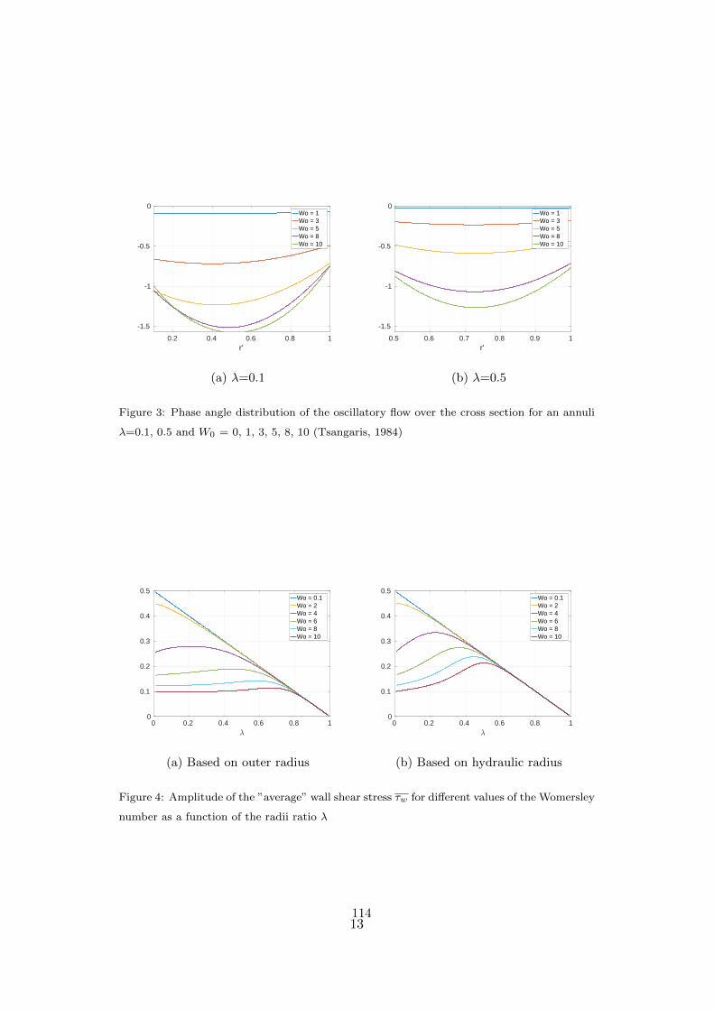
0.2 0.4 0.6 0.8 1r'

-1.5

-1

-0.5

0Wo = 1Wo = 3Wo = 5Wo = 8Wo = 10

(a) λ=0.1

0.5 0.6 0.7 0.8 0.9 1r'

-1.5

-1

-0.5

0Wo = 1Wo = 3Wo = 5Wo = 8Wo = 10

(b) λ=0.5

Figure 3: Phase angle distribution of the oscillatory flow over the cross section for an annuli

λ=0.1, 0.5 and W0 = 0, 1, 3, 5, 8, 10 (Tsangaris, 1984)

0 0.2 0.4 0.6 0.8 10

0.1

0.2

0.3

0.4

0.5Wo = 0.1Wo = 2Wo = 4Wo = 6Wo = 8Wo = 10

(a) Based on outer radius

0 0.2 0.4 0.6 0.8 10

0.1

0.2

0.3

0.4

0.5Wo = 0.1Wo = 2Wo = 4Wo = 6Wo = 8Wo = 10

(b) Based on hydraulic radius

Figure 4: Amplitude of the ”average” wall shear stress τw for different values of the Womersley

number as a function of the radii ratio λ

13114

• For a weakly unsteady flow, for instance Wo < 2, the amplitude of τw

varies in a quasi-linear way with the radius ratio λ.

• For a strongly unsteady flow, for instance Wo > 8, the amplitude of τw is

quasi-constant with a radius ratio λ between 0 and 0.5.190

• For λ > 0.8, the amplitude of τw remain the same regardless the nature

of the unsteady flow.

The velocity profile tend to exhibit a Poiseuille shape and loses its phase

lag with the pressure gradient. The more the annuli is confined, the more

the average wall shear stress τw of a quasi-steady flow approximation is195

valid.

Before proceeding further, please note that the definition of the Womersley

number used by Tsangaris (1984) for an annuli takes into account as a charac-

teristic length the outer radius of the annuli, neglecting the effect of the inner

radius. Thereafter, we define a local Womersley number based on the inner and200

the outer radius : a hydraulic radius. The hydraulic radius Rh was calculated

based on the cross-sectional area and wetted perimeter as

Rh = 2π(R2

s −R2c)

2π(Rc +Rs)= Rs −Rc (22)

The local Womersley number, Woh, is then equal to

Woh = (Rs −Rc)√ωρ

µ= Wo(1− λ) (23)

Therefore, the ”average” wall shear stress (21) is rescaled as a function of the

local Womersley number Woh.205

Figure 4b shows the variation of τw for different values of Woh as a function of

λ.

Remarks held previously remain invariable except that the amplitude of τw is

no longer quasi-constant with a radius ratio λ between 0 and 0.5. However,

the area of validity of the quasi-steady flow assumption noticed at Figure 4a210

has become wider in Figure (4b) by taking into account the inner radius. The

quasi-steady flow assumption is considered acceptable when the minimum value

14115

0 0.1 0.2 0.3 0.4Distance along the spine [m]

0

5

10

15R

adiu

s [m

m]

SCSC - 10th degree polynomial FittSSSSSS - 10th degree polynomial Fitt

Figure 5

of the radius ratio λ is around 0.6.

MRI data from the Visible Human Project (VHP) provide outlines of the cord

and of the SSS/dura interface at 49 sites along the spinal cord. At each cross-215

section, Bertram (2009) computed the area of each closed outline and the radius

of a circle having the same area was calculated. Figure 5 displays these results.

The radius ratio λ is computed based on these data. Except near the skull and

the base of the spine, hydraulic radius λ is greater than 0.6. It can be assumed

that when accounting for the CSF viscosity, the quasi-steady flow approximation220

for this area is acceptable.

15116

7. Acknowledgments

References

Berkouk, K., Carpenter, P.W., Lucey, A.D., 2003. Pressure wave propagation

in fluid-filled co-axial elastic tubes. Part 1: Basic theory. Journal of Biome-225

chanical Engineering 125, 852–856.

Bertram, C.D., 2009. A numerical investigation of waves propagating in

the spinal cord and subarachnoid space in the presence of a syrinx.

Journal of Fluids and Structures 25, 1189–1205. URL: http://www.

sciencedirect.com/science/article/pii/S0889974609000760, doi:10.230

1016/j.jfluidstructs.2009.06.008.

Bertram, C.D., Brodbelt, A.R., Stoodley, M.A., 2005. The origins of sy-

ringomyelia: numerical models of fluid/structure interactions in the spinal

cord. Journal of Biomechanical Engineering 127, 1099–1109.

Carpenter, P.W., Berkouk, K., Lucey, A.D., 2003. Pressure wave propagation235

in fluid-filled co-axial elastic tubes. Part 2: Mechanisms for the pathogenesis

of syringomyelia. Journal of Biomechanical Engineering 125, 857–863.

Cirovic, S., 2009. A coaxial tube model of the cerebrospinal fluid pulse propaga-

tion in the spinal column. Journal of Biomechanical Engineering 131, 021008.

doi:10.1115/1.3005159.240

Cirovic, S., Kim, M., 2012. A one-dimensional model of the spinal cerebrospinal-

fluid compartment. Journal of Biomechanical Engineering 134, 021005.

doi:10.1115/1.4005853.

Elliott, N.S.J., Lucey, A.D., Lockerby, D.A., Brodbelt, A.R., 2017. Fluid-

structure interactions in a cylindrical layered wave guide with application in245

the spinal column to syringomyelia. Journal of Fluids and Structures 70,

464–499. URL: http://www.sciencedirect.com/science/article/pii/

S088997461630158X, doi:10.1016/j.jfluidstructs.2016.11.007.

16117

Flanagan, M.F., 2015. The Role of the Craniocervical Junction in Craniospinal

Hydrodynamics and Neurodegenerative Conditions. Neurology Research In-250

ternational 2015, 794829. doi:10.1155/2015/794829.

Haughton, V., Mardal, K.A., 2014. Spinal fluid biomechanics and imaging: an

update for neuroradiologists. AJNR. American journal of neuroradiology 35,

1864–1869. doi:10.3174/ajnr.A4023.

Lockey, M.P., Poots, G., Williams, B., 1975. Theoretical aspects of the at-255

tenuation of pressure pulses within cerebrospinal-fluid pathways. Medical

and biological engineering 13, 861–869. URL: https://link.springer.com/

article/10.1007/BF02478090, doi:10.1007/BF02478090.

Loth, F., Yardimci, M.A., Alperin, N., 2001. Hydrodynamic modeling of cere-

brospinal fluid motion within the spinal cavity. Journal of Biomechanical260

Engineering 123, 71–79.

Luciano, M., Dombrowski, S., 2007. Hydrocephalus and the heart: interactions

of the first and third circulations. Cleveland Clinic Journal of Medicine 74

Suppl 1, S128–131.

Sakka, L., Coll, G., Chazal, J., 2011. Anatomy and physiology of cerebrospinal265

fluid. European Annals of Otorhinolaryngology, Head and Neck Diseases 128,

309–316. doi:10.1016/j.anorl.2011.03.002.

Tsangaris, 1984. Oscillatory flow of an incompressible, viscous fluid in a straight

annular pipe<br/>. Journal de mcanique thorique et applique 3, 467–478.

URL: http://www.refdoc.fr/Detailnotice?idarticle.270

VHP, . The National Library of Medicines Visible Human Project. URL: https:

//www.nlm.nih.gov/research/visible/visible_human.html.

Womersley, J.R., 1955. Mathematical theory of oscillating flow in an elastic

tube. The Journal of Physiology 127, 37–38P.

17118

Zagzoule, M., Marc-Vergnes, J.P., 1986. A global mathematical model of the275

cerebral circulation in man. Journal of Biomechanics 19, 1015–1022.

18119

Appendix D

CSF cervical flow computed from1D model vs. MRI Data

The following poster was presented during the 8th World Congress of Biomechanics held from8 to 12 July, 2018 in Dublin Ireland

121

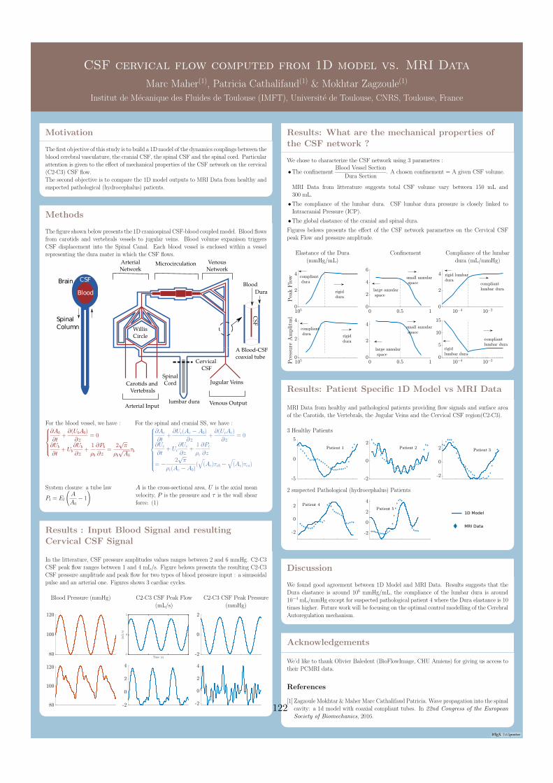
LATEX TikZposter

CSF cervical flow computed from 1D model vs. MRI Data

Marc Maher(1), Patricia Cathalifaud(1) & Mokhtar Zagzoule(1)

Institut de Mecanique des Fluides de Toulouse (IMFT), Universite de Toulouse, CNRS, Toulouse, France

CSF cervical flow computed from 1D model vs. MRI Data

Marc Maher(1), Patricia Cathalifaud(1) & Mokhtar Zagzoule(1)

Institut de Mecanique des Fluides de Toulouse (IMFT), Universite de Toulouse, CNRS, Toulouse, France

Motivation

The first objective of this study is to build a 1D model of the dynamics couplings between theblood cerebral vasculature, the cranial CSF, the spinal CSF and the spinal cord. Particularattention is given to the effect of mechanical properties of the CSF network on the cervical(C2-C3) CSF flow.The second objective is to compare the 1D model outputs to MRI Data from healthy andsuspected pathological (hydrocephalus) patients.

Methods

The figure shown below presents the 1D craniospinal CSF-blood coupled model. Blood flowsfrom carotids and vertebrals vessels to jugular veins. Blood volume expanison triggersCSF displacement into the Spinal Canal. Each blood vessel is enclosed within a vesselrepresenting the dura mater in which the CSF flows.

CSF

Blood

Brain

Spinal

Column WillisCircle

Jugular VeinsCarotids and Vertebrals

Cervical CSF

Spinal Cord

lumbar dura

Dura

Blood

CSF

A Blood-CSF coaxial tube

Arterial InputVenous Output

Arterial Network

Microcirculation Venous Network

For the blood vessel, we have :

∂Ab

∂t+∂(UbAb)

∂z= 0

∂Ub∂t

+ Ub∂Ub∂z

+1

ρb

∂Pb∂z

=2√π

ρb√Abτb

For the spinal and cranial SS, we have :

∂Ac

∂t+∂Uc(Ac − Ab)

∂z+∂(UcAc)

∂z= 0

∂Uc∂t

+ Uc∂Uc∂z

+1

ρc

∂Pc∂z

= − 2√π

ρc(Ac − Ab)(√

(Ac)τcb −√

(Ac)τcs)

System closure: a tube law

Pt = El

(A

A0− 1

) A is the cross-sectional area, U is the axial meanvelocity, P is the pressure and τ is the wall shearforce. (1)

Results : Input Blood Signal and resulting

Cervical CSF Signal

In the litterature, CSF pressure amplitudes values ranges between 2 and 6 mmHg. C2-C3CSF peak flow ranges between 1 and 4 mL/s. Figure belows presents the resulting C2-C3CSF pressure amplitude and peak flow for two types of blood pressure input : a sinusoidalpulse and an arterial one. Figures shows 3 cardiac cycles.

Blood Pressure (mmHg) C2-C3 CSF Peak Flow(mL/s)

C2-C3 CSF Peak Pressure(mmHg)

Results: What are the mechanical properties of

the CSF network ?

We chose to characterize the CSF network using 3 parametres :

•The confinementBlood Vessel Section

Dura Section. A chosen confinement = A given CSF volume.

MRI Data from litterature suggests total CSF volume vary between 150 mL and300 mL.

•The compliance of the lumbar dura. CSF lumbar dura pressure is closely linked toIntracranial Pressure (ICP).

•The global elastance of the cranial and spinal dura.

Figures belows presents the effect of the CSF network parametres on the Cervical CSFpeak Flow and pressure amplitude.

Elastance of the Dura(mmHg/mL)

Confinement Compliance of the lumbardura (mL/mmHg)

Results: Patient Specific 1D Model vs MRI Data

MRI Data from healthy and pathological patients providing flow signals and surface areaof the Carotids, the Vertebrals, the Jugular Veins and the Cervical CSF region(C2-C3).

3 Healthy Patients

2 suspected Pathological (hydrocephalus) Patients

1D Model

MRI Data

Discussion

We found good agreement between 1D Model and MRI Data. Results suggests that theDura elastance is around 106 mmHg/mL, the compliance of the lumbar dura is around10−4 mL/mmHg except for suspected pathological patient 4 where the Dura elastance is 10times higher. Future work will be focusing on the optimal control modelling of the CerebralAutoregulation mechanism.

Acknowledgements

We’d like to thank Olivier Baledent (BioFlowImage, CHU Amiens) for giving us access totheir PCMRI data.

References

[1] Zagzoule Mokhtar & Maher Marc Cathalifaud Patricia. Wave propagation into the spinalcavity: a 1d model with coaxial compliant tubes. In 22nd Congress of the EuropeanSociety of Biomechanics, 2016.

122

Bibliography

[1] Lazorthes Guy 1910-2014. Vascularisation et circulation de l’encephale. Tome I. Anatomiedescriptive et fonctionnelle. fre. Paris New York Barcelone: Masson, 1976 (cit. on p. 20).

[2] Andreas A. Linninger et al. “Cerebrospinal Fluid Mechanics and Its Coupling to Cere-brovascular Dynamics.” In: Annual Review of Fluid Mechanics 48 (2016), pp. 219–257(cit. on pp. 47, 60, 61).

[3] N. Alperin et al. “Automated Quantitation of Spinal CSF Volume and Measurementof Craniospinal CSF Redistribution Following Lumbar Withdrawal in Idiopathic In-tracranial Hypertension.” In: American Journal of Neuroradiology 37.10 (Oct. 2016),pp. 1957–1963 (cit. on p. 57).

[4] Noam Alperin et al. “From Cerebrospinal Fluid Pulsation to Noninvasive IntracranialCompliance and Pressure Measured by MRI Flow Studies.” In: Current Medical ImagingReviews 2.1 (Feb. 1, 2006), pp. 117–129 (cit. on p. 57).

[5] O. Balédent, M. C. Henry-Feugeas, and I. Idy-Peretti. “Cerebrospinal Fluid Dynamicsand Relation with Blood Flow: A Magnetic Resonance Study with SemiautomatedCerebrospinal Fluid Segmentation.” In: Investigative Radiology 36.7 (July 2001), pp. 368–377. pmid: 11496092 (cit. on pp. 47, 61, 64, 65).

[6] Olivier Balédent et al. “Relationship between Cerebrospinal Fluid and Blood Dynamics inHealthy Volunteers and Patients with Communicating Hydrocephalus.” In: InvestigativeRadiology 39.1 (Jan. 2004), pp. 45–55 (cit. on p. 62).

[7] C. D. Bertram. “A Numerical Investigation of Waves Propagating in the Spinal Cord andSubarachnoid Space in the Presence of a Syrinx.” In: Journal of Fluids and Structures25.7 (2009), pp. 1189–1205 (cit. on p. 24).

[8] C. D. Bertram, A. R. Brodbelt, and M. A. Stoodley. “The Origins of Syringomyelia:Numerical Models of Fluid/Structure Interactions in the Spinal Cord.” In: Journal ofBiomechanical Engineering 127.7 (Dec. 2005), pp. 1099–1109 (cit. on p. 24).

[9] C. D. Bertram and M. Heil. “A Poroelastic Fluid/Structure-Interaction Model of Cere-brospinal Fluid Dynamics in the Cord With Syringomyelia and Adjacent Subarachnoid-Space Stenosis.” In: Journal of Biomechanical Engineering 139.1 (Jan. 2017) (cit. onp. 25).

[10] Lynne E. Bilston and Lawrence E. Thibault. “The Mechanical Properties of the HumanCervical Spinal cordIn Vitro.” In: Annals of Biomedical Engineering 24.1 (Sept. 1, 1995),pp. 67–74 (cit. on p. 25).

[11] P. D. Brown et al. “Molecular Mechanisms of Cerebrospinal Fluid Production.” In:Neuroscience 129.4 (2004), pp. 957–970 (cit. on p. 15).

[12] Suncica Canic and Eun Heui Kim. “Mathematical Analysis of the Quasilinear Effectsin a Hyperbolic Model Blood Flow through Compliant Axi-Symmetric Vessels.” In:Mathematical Methods in the Applied Sciences 26.14 (2003), pp. 1161–1186 (cit. onp. 27).

123

[13] Gregory S. H. Chan et al. “Contribution of Arterial Windkessel in Low-FrequencyCerebral Hemodynamics during Transient Changes in Blood Pressure.” In: Journal ofApplied Physiology 110.4 (Feb. 3, 2011), pp. 917–925 (cit. on p. 49).

[14] Dorian Chauvet et al. “Histological and Biomechanical Study of Dura Mater Appliedto the Technique of Dura Splitting Decompression in Chiari Type I Malformation.” In:Neurosurgical Review 33.3 (July 2010), 287–294; discussion 295. pmid: 20440557 (cit. onp. 25).

[15] Srdjan Cirovic and Minsuok Kim. “A One-Dimensional Model of the Spinal Cerebrospinal-Fluid Compartment.” In: Journal of Biomechanical Engineering 134.2 (Feb. 2012),p. 021005 (cit. on pp. 25, 33).

[16] Marek Czosnyka et al. “Cerebrospinal Fluid Dynamics.” In: Physiological Measurement25.5 (Oct. 2004), R51–76. pmid: 15535175 (cit. on pp. 47, 61).

[17] Helle H. Damkier, Peter D. Brown, and Jeppe Praetorius. “Cerebrospinal Fluid Secretionby the Choroid Plexus.” In: Physiological Reviews 93.4 (Oct. 2013), pp. 1847–1892 (cit. onpp. 12, 15).

[18] Dries De Kegel et al. “Biomechanical Characterization of Human Dura Mater.” In:Journal of the Mechanical Behavior of Biomedical Materials 79 (Mar. 1, 2018), pp. 122–134 (cit. on p. 25).

[19] Florian Doepp et al. “How Does the Blood Leave the Brain? A Systematic UltrasoundAnalysis of Cerebral Venous Drainage Patterns.” In: Neuroradiology 46.7 (July 2004),pp. 565–570. pmid: 15258709 (cit. on p. 65).

[20] Zakaria Doulfoukar et al. “Méthode numérique pour la résolution de l’écoulement d’unfluide viscoélastique en conduite à paroi déformable.” In: Journal de Physique III 6.3(Mar. 1, 1996), pp. 433–442 (cit. on p. 31).

[21] Steffi Dreha-Kulaczewski et al. “Respiration and the Watershed of Spinal CSF Flow inHumans.” In: Scientific Reports 8.1 (Apr. 4, 2018), p. 5594 (cit. on p. 15).

[22] Michael Egnor et al. “The Cerebral Windkessel and Its Relevance to Hydrocephalus:The Notch Filter Model of Cerebral Blood Flow.” In: Cerebrospinal Fluid Research 3(Suppl 1 Dec. 21, 2006), S48. pmid: null (cit. on p. 49).

[23] D. R. Enzmann and N. J. Pelc. “Brain Motion: Measurement with Phase-Contrast MRImaging.” In: Radiology 185.3 (Dec. 1992), pp. 653–660 (cit. on p. 23).

[24] D. R. Enzmann and N. J. Pelc. “Cerebrospinal Fluid Flow Measured by Phase-ContrastCine MR.” In: AJNR Am J Neuroradiol 14.6 (Dec. 1993), 1301–1307; discussion 1309–1310 (cit. on pp. 15, 23, 47, 61, 65).

[25] D. A. Frankel, D. P. Fessell, and W. P. Wolfson. “High Resolution Sonographic De-termination of the Normal Dimensions of the Intracranial Extraaxial Compartment inthe Newborn Infant.” In: Journal of Ultrasound in Medicine: Official Journal of theAmerican Institute of Ultrasound in Medicine 17.7 (July 1998), 411–415; quiz 417–418.pmid: 9669298 (cit. on p. 23).

124

[26] M. Freund et al. “[Measurement of CSF flow in the spinal canal using MRI with anoptimized MRI protocol: experimental and clinical studies].” In: Rofo 173.4 (Apr. 2001),pp. 306–314 (cit. on p. 15).

[27] James E. Galford and James H. McElhaney. “A Viscoelastic Study of Scalp, Brain, andDura.” In: Journal of Biomechanics 3.2 (Mar. 1, 1970), pp. 211–221 (cit. on p. 25).

[28] D. Greitz et al. “Pulsatile Brain Movement and Associated Hydrodynamics Studiedby Magnetic Resonance Phase Imaging. The Monro-Kellie Doctrine Revisited.” In:Neuroradiology 34.5 (1992), pp. 370–380. pmid: 1407513 (cit. on p. 15).

[29] Sumeet Gupta et al. “Three-Dimensional Computational Modeling of Subject-SpecificCerebrospinal Fluid Flow in the Subarachnoid Space.” In: Journal of BiomechanicalEngineering 131.2 (Feb. 2009), p. 021010 (cit. on p. 48).

[30] Leszek Herbowski. “The Maze of the Cerebrospinal Fluid Discovery.” In: AnatomyResearch International. 2013 (cit. on p. 2).

[31] J.V. Hickey. Clinical Practice of Neurological and Neurosurgical Nursing. Wolters KluwerHealth, 2011 (cit. on p. 4).

[32] O. Hunziker and A. Schweizer. “Postmortem changes in stereological parameters ofcerebral capillaries.” eng. In: Beiträge zur Pathologie: "Aschoff’s" Journal 161.3 (1977),pp. 244–255 (cit. on p. 20).

[33] Zaamin B Hussain, Amaani B Hussain, and Patrick Mitchell. “Extra-Axial CerebrospinalFluid Spaces in Children with Benign External Hydrocephalus: A Case-Control Study.”In: The Neuroradiology Journal 30.5 (Oct. 2017), pp. 410–417. pmid: 28691570 (cit. onp. 23).

[34] Conrad E. Johanson et al. “Multiplicity of Cerebrospinal Fluid Functions: New Challengesin Health and Disease.” In: Cerebrospinal Fluid Research 5 (May 2008), p. 10 (cit. onp. 12).

[35] Miles Johnston et al. “Evidence of Connections between Cerebrospinal Fluid and NasalLymphatic Vessels in Humans, Non-Human Primates and Other Mammalian Species.”In: Cerebrospinal Fluid Research 1 (Dec. 2004), p. 2 (cit. on p. 12).

[36] Wojciech Kalata et al. “MR Measurement of Cerebrospinal Fluid Velocity Wave Speedin the Spinal Canal.” In: IEEE transactions on bio-medical engineering 56.6 (June 2009),pp. 1765–1768 (cit. on p. 59).

[37] Yi-Hsuan Kao et al. “The Respiratory Modulation of Intracranial Cerebrospinal FluidPulsation Observed on Dynamic Echo Planar Images.” In: Magnetic Resonance Imaging26.2 (Feb. 2008), pp. 198–205 (cit. on p. 15).

[38] W. W. Lam et al. “Ultrasonographic Measurement of Subarachnoid Space in NormalInfants and Children.” In: Pediatric Neurology 25.5 (Nov. 2001), pp. 380–384. pmid:11744312 (cit. on p. 23).

[39] G Lazorthes. “Arterial vascularization of the brain stem. Research technic and newdata.” fre. In: Bulletin de l’Academie nationale de medecine 149.30 (1965) (cit. on p. 20).

125

[40] M. Libicher and J. Tröger. “US Measurement of the Subarachnoid Space in Infants:Normal Values.” In: Radiology 184.3 (Sept. 1992), pp. 749–751. pmid: 1509061 (cit. onp. 23).

[41] Andreas A. Linninger et al. “A Mathematical Model of Blood, Cerebrospinal Fluid andBrain Dynamics.” In: Journal of Mathematical Biology 59.6 (2009), pp. 729–759 (cit. onp. 6).

[42] F. Loth, M. A. Yardimci, and N. Alperin. “Hydrodynamic Modeling of CerebrospinalFluid Motion within the Spinal Cavity.” In: Journal of Biomechanical Engineering 123.1(Feb. 2001), pp. 71–79 (cit. on pp. 48, 55).

[43] Mark Luciano and Stephen Dombrowski. “Hydrocephalus and the Heart: Interactions ofthe First and Third Circulations.” In: Cleveland Clinic Journal of Medicine 74 Suppl 1(Feb. 2007), S128–131. pmid: 17455561 (cit. on pp. 49, 61).

[44] Melody P. Lun, Edwin S. Monuki, and Maria K. Lehtinen. “Development and Functionsof the Choroid Plexus–Cerebrospinal Fluid System.” In: Nature reviews. Neuroscience16.8 (Aug. 2015), pp. 445–457 (cit. on p. 12).

[45] Jason T. Maikos, Ragi A. I. Elias, and David I. Shreiber. “Mechanical Properties ofDura Mater from the Rat Brain and Spinal Cord.” In: Journal of Neurotrauma 25.1 (Jan.2008), pp. 38–51. pmid: 18355157 (cit. on p. 25).

[46] Edward L. Mazuchowski and Lawrence E. Thibault. “BIOMECHANICAL PROPERTIESOF THE HUMAN SPINAL CORD AND PIA MATER.” In: (cit. on p. 25).

[47] C. B. McArdle et al. “Developmental Features of the Neonatal Brain: MR Imaging. PartII. Ventricular Size and Extracerebral Space.” In: Radiology 162 (1 Pt 1 Jan. 1987),pp. 230–234. pmid: 3786768 (cit. on p. 23).

[48] B. Mokri. “The Monro-Kellie Hypothesis: Applications in CSF Volume Depletion.” In:Neurology 56.12 (June 26, 2001), pp. 1746–1748. pmid: 11425944 (cit. on p. 16).

[49] Nejat Narli et al. “Ultrasonographic Measurement of Subarachnoid Space in NormalTerm Newborns.” In: European Journal of Radiology 58.1 (Apr. 2006), pp. 110–112.pmid: 16406435 (cit. on p. 23).

[50] Frank H. Netter. Atlas of Human Anatomy. Elsevier Health Sciences, Dec. 19, 2017.674 pp. (cit. on pp. 11, 14–16).

[51] Neuroscience. 2nd. Sinauer Associates, 2001 (cit. on p. 10).[52] Hiroshi Ozawa et al. “Mechanical Properties and Function of the Spinal Pia Mater.” In:

Journal of Neurosurgery. Spine 1.1 (July 2004), pp. 122–127. pmid: 15291032 (cit. onp. 25).

[53] Soroush Heidari Pahlavian et al. “The Impact of Spinal Cord Nerve Roots and DenticulateLigaments on Cerebrospinal Fluid Dynamics in the Cervical Spine.” In: PLOS ONE 9.4(Apr. 2014), e91888 (cit. on p. 48).

[54] Dennis Patin et al. “Anatomic and Biomechanical Properties of Human Lumbar DuraMater.” In: Anesthesia & Analgesia 76.3 (Mar. 1, 1993), pp. 535–540. pmid: 8452262(cit. on p. 25).

126

[55] T. J. Pedley. The Fluid Mechanics of Large Blood Vessels by T. J. Pedley. Apr. 1980.(Visited on 05/13/2019) (cit. on p. 31).

[56] Michael Pollay. “The Function and Structure of the Cerebrospinal Fluid Outflow System.”In: Cerebrospinal Fluid Research 7 (June 2010), p. 9 (cit. on p. 12).

[57] P. Prassopoulos and D. Cavouras. “CT Evaluation of Normal CSF Spaces in Children:Relationship to Age, Gender and Cranial Size.” In: European Journal of Radiology 18.1(Feb. 1, 1994), pp. 22–25 (cit. on p. 23).

[58] Alfio Quarteroni and Luca Formaggia. “Mathematical Modelling and Numerical Sim-ulation of the Cardiovascular System.” In: Handbook of Numerical Analysis. Vol. 12.Computational Models for the Human Body. Elsevier, Jan. 1, 2004, pp. 3–127 (cit. onp. 31).

[59] Adnan I. Qureshi et al. “Patterns and Rates of Supplementary Venous Drainage to theInternal Jugular Veins.” In: Journal of Neuroimaging: Official Journal of the AmericanSociety of Neuroimaging 26.4 (July 2016), pp. 445–449. pmid: 26888667 (cit. on p. 65).

[60] Leonardo Rangel-Castillo, Shankar Gopinath, and Claudia S. Robertson. “Managementof Intracranial Hypertension.” In: Neurologic Clinics 26.2 (2008). Neurologic CriticalCare, pp. 521 –541 (cit. on p. 4).

[61] G. Rodríguez-Boto et al. “Basic concepts about brain pathophysiology and intracranialpressure monitoring.” In: Neurología (English Edition) 30.1 (2015), pp. 16–22 (cit. onpp. 3, 47).

[62] M. Runza et al. “Lumbar Dura Mater Biomechanics: Experimental Characterizationand Scanning Electron Microscopy Observations.” In: Anesthesia and Analgesia 88.6(June 1999), pp. 1317–1321. pmid: 10357337 (cit. on p. 25).

[63] L. Sakka, G. Coll, and J. Chazal. “Anatomy and Physiology of Cerebrospinal Fluid.”In: Eur Ann Otorhinolaryngol Head Neck Dis 128.6 (Dec. 2011), pp. 309–316 (cit. onpp. 12, 57).

[64] Diego San Millán Ruíz et al. “The Craniocervical Venous System in Relation to CerebralVenous Drainage.” In: AJNR. American journal of neuroradiology 23.9 (Oct. 2002),pp. 1500–1508. pmid: 12372739 (cit. on p. 65).

[65] Mansoor Sharifi et al. “The Choroid Plexus of the Fourth Ventricle and Its Arteries.” In:Folia Morphologica 64.3 (Aug. 2005), pp. 194–198 (cit. on p. 12).

[66] Spencer Sherwin et al. “Computational Modeling of 1D Blood Flow with VariableMechanical Properties and Application to the Simulation of Wave Propagation in theHuman Arterial System.” In: Int. J. Numer. Meth. Fluids 43 (Oct. 2003), pp. 673–700(cit. on p. 31).

[67] Yubing Shi, Patricia Lawford, and Rodney Hose. “Review of Zero-D and 1-D Models ofBlood Flow in the Cardiovascular System.” In: BioMedical Engineering OnLine 10 (Apr.2011), p. 33 (cit. on p. 31).

[68] T. Speake et al. “Mechanisms of CSF Secretion by the Choroid Plexus.” In: MicroscopyResearch and Technique 52.1 (Jan. 1, 2001), pp. 49–59. pmid: 11135448 (cit. on p. 12).

127

[69] Souraya Stoquart-Elsankari et al. “A Phase-Contrast MRI Study of Physiologic CerebralVenous Flow.” In: Journal of Cerebral Blood Flow and Metabolism: Official Journalof the International Society of Cerebral Blood Flow and Metabolism 29.6 (June 2009),pp. 1208–1215. pmid: 19352399 (cit. on p. 65).

[70] Mark E. Wagshul, Per K. Eide, and Joseph R. Madsen. “The Pulsating Brain: A Reviewof Experimental and Clinical Studies of Intracranial Pulsatility.” In: Fluids and Barriersof the CNS 8 (Jan. 2011), p. 5 (cit. on p. 15).

[71] Nico Westerhof, Jan-Willem Lankhaar, and Berend E. Westerhof. “The Arterial Wind-kessel.” In: Medical & Biological Engineering & Computing 47.2 (Feb. 1, 2009), pp. 131–141 (cit. on p. 49).

[72] K. Zagórska-Swiezy et al. “Arterial Supply and Venous Drainage of the Choroid Plexusof the Human Lateral Ventricle in the Prenatal Period as Revealed by Vascular CorrosionCasts and SEM.” In: Folia Morphologica 67.3 (Aug. 2008), pp. 209–213 (cit. on p. 12).

[73] M. Zagzoule and J. P. Marc-Vergnes. “A Global Mathematical Model of the CerebralCirculation in Man.” In: J Biomech 19.12 (1986), pp. 1015–1022 (cit. on pp. 7, 16, 19–21,37).

[74] Rui Zou et al. “Intracranial pressure waves: Characterization of a pulsation absorber withnotch filter properties using systems analysis - Laboratory investigation.” In: Journal ofNeurosurgery: Pediatrics 2.1 (July 2008), pp. 83–94. pmid: 18590402 (cit. on p. 49).

128