A numerical study of the western Cosmonaut polynya in a coupled ocean-sea ice model

A numerical study of the western Cosmonaut polynya in a coupled

ocean––sea ice model

T. G. Prasad1 and Julie L. McClean2

Department of Oceanography, Naval Postgraduate School, Monterey, California, USA

Elizabeth C. HunkeTheoretical Division, Los Alamos National Laboratory, Los Alamos, New Mexico, USA

Albert J. Semtner and Detelina IvanovaDepartment of Oceanography, Naval Postgraduate School, Monterey, California, USA

Received 22 December 2004; revised 15 April 2005; accepted 23 May 2005; published 8 October 2005.

[1] Employing results from a 0.4�, 40-level fully global, coupled ocean–sea ice model,we investigated the role of physical processes emanating from atmosphere, ocean, and icein the initiation, maintenance, and termination of a sensible heat polynya with a focus onthe western Cosmonaut polynya that occurred during May–July 1999. The Cosmonautpolynya first appeared in early May 1999 in the form of an ice-free embayment,transformed into an enclosed polynya on 5–9 July, and disappeared by late July, when theice from the surrounding regions began to encircle the embayment. Except for thedifferences in ice concentrations, the time of appearance, size, and shape of the Cosmonautpolynya simulated by the model are in approximate agreement with the Special SensorMicrowave/Imager (SSM/I) observations. Between May and July 1999 the CosmonautSea experienced two synoptic storms, both lasting �5 days. Followed by the passage ofthe first storm on 12–19 June, there was a remarkable growth in the size of theembayment by 21 � 103 km2. Associated with this, the sea surface temperature (SST) roseby 0.15�C, the upward heat flux jumped from 5 to 94 W m�2, and a net freshwaterflux into the ocean increased by 2 cm d�1. By running the model simulation with a 20%wind speed increase, it is demonstrated that the twofold increase in SST and upwardheat flux increased the embayment area by 15 � 103 km2 and decreased the iceconcentration by approximately 10% from the control run. A similar, but somewhatweaker wind event that took place on 30 June to 10 July had less influence on theembayment area although the upward heat flux (65 W m�2) was comparable tothe first event. By examining the vertical displacement of the �1.6�C isotherm depthprior to, during, and after these two storms, we demonstrate that the impetus provided bythese storms was able to raise the �1.6�C isotherm depth by 30 m through wind-drivenmixing, making sufficient oceanic heat input from beneath the mixed layer availableto prevent freezing and/or delay ice formation while ice in the adjacent regions continuedto grow. A sudden shift in the ice drift direction from southwest to northeast (3 July)followed by the second storm, accompanied by large air-sea temperature differences,caused the enclosure of the embayment, subsequent formation of the polynya, andits termination.

Citation: Prasad, T. G., J. L. McClean, E. C. Hunke, A. J. Semtner, and D. Ivanova (2005), A numerical study of the western

Cosmonaut polynya in a coupled ocean–sea ice model, J. Geophys. Res., 110, C10008, doi:10.1029/2004JC002858.

1. Introduction

[2] Sea ice plays an important role in the global climatesystem by influencing regional polar heat and freshwaterbudgets, surface albedo, and consequently the oceanic andatmospheric circulation. Polynyas are areas of persistentopen water or reduced ice concentration surrounded by seaice [Smith et al., 1990; Morales Maqueda et al., 2004].Polynyas have been divided into two classes: ‘‘sensible

JOURNAL OF GEOPHYSICAL RESEARCH, VOL. 110, C10008, doi:10.1029/2004JC002858, 2005

1Now at Department of Marine Science, University of SouthernMississippi, Stennis Space Center, Mississippi, USA.

2Now at Scripps Institution of Oceanography, University of California,San Diego, La Jolla, California, USA.

This paper is not subject to U.S. copyright.Published in 2005 by the American Geophysical Union.

C10008 1 of 21

heat’’ and ‘‘latent heat’’ according to their formation mech-anism and maintenance. Sensible heat polynyas are ther-mally driven. They appear as a result of oceanic sensibleheat entering the area of polynya formation in amounts largeenough to melt any preexisting ice and prevent the growthof new ice. Latent heat polynyas are mechanically driven,and are created in areas where the ice motion is divergentdue to the prevailing winds or oceanic currents (for a reviewof polynyas, see Morales Maqueda et al. [2004]). Deepocean sensible heat polynyas constitute some 2% of theoverall Antarctic winter sea ice cover [Arbetter et al., 2004]and are responsible for the ventilation of warm deep waters[Comiso and Gordon, 1996]. Polynyas are important toclimate variability in that they impact the atmosphericcirculation, the ice variability, and regional primary produc-tion in coastal polynyas [Arrigo and van Dijken, 2003].Open water within the ice pack is often the location ofenhanced exchange of heat and moisture from the ocean tothe atmosphere. Thermal plumes of warm, moist air from arecurring polynya produce cloud formations that canachieve great heights. Recurring polynyas suggest consis-tency in their formation and maintenance, which would bemanifested in the evolution of the spatial structure of the seaice cover. Although, studies of these polynyas have revealedsome understanding of the crucial mechanisms, the ocean-ographic setting relevant to the polynya formation andmaintenance is not well understood.[3] A persistent region of reduced sea ice concentration in

the Cosmonaut Sea (Figure 1) was first reported by Comisoand Gordon [1987] who named it the Cosmonaut polynya.Later, with the advent of Special Sensor Microwave/Imager(SSM/I), Comiso and Gordon [1996] documented thespatial and temporal variability of the Cosmonaut polynyafrom sea ice concentration maps for several years (1987–1993). Recurring polynyas were observed in the eastern andwestern regions of this sea and were designated eastern andwestern Cosmonaut polynya (ECP and WCP), respectively.The ECP occurs near Cape Ann (Figure 1) one or moretimes during winter (July to October) while the WCP occurswest of 45�E in early winter. On occasion, the ECP andWCP occur at the same time and coalesce.[4] The formation of the ECP in the vicinity of Cape Ann

may be due to oceanic forcing [Comiso and Gordon, 1996]

or divergent winds [Arbetter et al., 2004; Bailey et al.,2004], or both. From the SSM/I observations, Comiso andGordon [1996] observed coastal polynyas forming adjacentto Cape Ann that grew in size and extended offshore. Usingclimatological data, they argued that this offshore locationexperienced upwelling of warm salty Circumpolar DeepWater resulting from the compression of the westwardflowing coastal current and the southern edge of theeastward flowing Antarctic Circumpolar Current via con-servation of potential vorticity. This water inhibited sea icegrowth resulting in polynya growth. While the vorticityconservation theory can be used to explain the mechanismof ECP formation because of its proximity to Cape Ann(Figure 1), the exact mechanisms causing the WCP forma-tion are unclear and have not been studied. This study willfocus on the forcing mechanisms responsible for thepreconditioning, formation, and maintenance of the WCP.Arbetter et al. [2004] investigated the processes of forma-tion, maintenance, and decay of a polynya using a 13-yearclimatology of atmospheric fields. They suggest thatatmospheric divergence may play a stronger role thanupwelling in initiating the surface divergence of sea ice inthis region.[5] There have been many attempts to model polynyas

in the Southern Ocean during the past two decades. Thesestudies have used regional or global models of varyingcomplexity with an active/passive atmosphere or ocean.An excellent review of these and other previous model-ing studies of the Weddell polynya are provided byMorales Maqueda et al. [2004]. Bailey et al. [2004]using a regional coupled atmosphere–sea ice modelstudied the formation mechanisms of the Cosmonautpolynya that occurred during 6–8 August 1988. Thesize, shape and intensity of their simulated polynya weredifferent from the SSM/I observations (compare theirFigures 4 and 5). This model-data discrepancy couldbe associated with the lack of realistic ocean currentsand oceanic heat flux; both of these fields were specifiedin their simulation. Arbetter et al. [2004] and Bailey etal. [2004] emphasized the importance of the oceanicprocesses in maintaining the Cosmonaut polynyas, butthey were unable to address it directly. It is this issuethat we would like to address here.[6] This builds on prior work, most notably that of

Comiso and Gordon [1996], Arbetter et al. [2004], andBailey et al. [2004]. By using a coupled ocean–sea icemodel, we are able to provide direct insight into oceanprocesses, something the prior studies were unable to do.We employ a coupled ocean–sea ice model of moderatelyhigh resolution that includes an active ocean and icedynamics and thermodynamics. Our preliminary model-data comparisons suggest that the model is capable ofsimulating the Cosmonaut polynyas for different years.For example, consistent with the SSM/I observations, aWCP occurred in 2002. In this study, we focus on the WCPthat occurred during May–July 1999. In the ensuingsections, the Cosmonaut polynya refers to the WCP unlessotherwise stated. We chose this period because the Cosmo-naut polynya that occurred during May–July 1999 (1) waspreceded by the largest embayment in the last two decades,(2) lasted for several weeks between the time it appearedand disappeared, and (3) experienced the passage of two

Figure 1. Map of the Antarctic study region (90�W to90�E, 90�–50�S) showing bathymetry (shaded) and theCosmonaut Sea, Cape Ann, Maud Rise, and Weddell Sea.

C10008 PRASAD ET AL.: MECHANISMS FOR COSMONAUT POLYNYA

2 of 21

C10008

synoptic storm events, which enabled us to study theresponse of the upper ocean and sea ice to storm events.The present coupled model with the advantage of havingrealistic ocean dynamics shows a considerable improve-ment in simulated polynya structure and variability. We tryto address the following questions: (1) What are themechanisms that initiate and maintain the embayment?(2) What are the mechanisms involved in transforming anembayment into the Cosmonaut polynya? (3) What are themechanisms leading to its decay?[7] The paper is organized as follows. A brief description

of the coupled ocean–sea ice model and the forcing fieldsare provided in section 2. We present the evolution of theCosmonaut polynya that occurred between May and July1999 using SSM/I sea ice concentrations and relate theatmospheric forcing fields to the timing of the observedpolynya in section 3. Model experiments are discussed insection 3.1. The role of ice and oceanic forcing ininitiating, maintaining and terminating the embayment/polynya are discussed respectively in sections 4 and 5.This is followed by a discussion (section 6) and summary(section 7) of the results.

2. Coupled Ocean–Sea Ice Model

[8] The simulation was performed with an ocean–sea icecoupled model developed at Los Alamos National Labora-tory, forced by realistic atmospheric reanalysis data. Detaileddocumentation for the ocean and ice models is given bySmith and Gent [2002], Hunke and Lipscomb [2004], Hunkeet al. [2004], and other publications referenced below.[9] The Parallel Ocean Program (POP) [Smith et al.,

1992; Dukowicz et al., 1993, 1994] is a z-coordinate oceanmodel featuring an implicit free surface; it solves theprimitive equations for temperature, salinity and the hori-zontal velocity components. The K-profile parameterization(KPP) [Large et al., 1994] provides vertical mixing ofmomentum and tracers, while convective adjustment occursthrough a high vertical diffusion coefficient done implicitlyin time. Horizontal friction is biharmonic with a coefficientof 1012 m4 s�1. The ocean model provides sea surfacetemperature, salinity, currents, and slope as well as afreezing or melting potential to the ice model. The freezingtemperature is salinity-dependent.[10] The Los Alamos Sea Ice Model (CICE) features

the elastic-viscous-plastic ice dynamics of Hunke andDukowicz [1997, 2002] and the energy conservingthermodynamics model of Bitz and Lipscomb [1999], witha nonlinear vertical salinity profile. A new incrementalremapping scheme [Lipscomb and Hunke, 2004] is usedfor horizontal advection, and mechanical redistribution ofice is accomplished through an energy-conserving ridgingscheme based on Thorndike et al. [1975]. There are fourlayers of ice and one layer of snow in each of five icethickness categories. Surface fluxes and temperatures arecomputed separately for each category and merged on thebasis of the fractional area covered by that category.Prognostic variables for each thickness category includeice area fraction, ice volume, ice energy in each verticallayer, snow volume and energy, and surface temperature.The ice model provides a freshwater flux, net heat fluxand ice-ocean stress to the ocean model. Details pertaining

to the CICE model are given by Hunke and Lipscomb[2004].[11] The ice and ocean models are coupled through a

driver that also reads atmospheric data from files andprepares the data for use by the other components. Thedriver merges ice and ocean quantities on the basis of the icearea fraction in cells where there is less than 100% icecoverage. The ice-ocean model runs as a single executable;the driver and ice model use a time step of 30 minutes,while the ocean model takes 48 leapfrog time steps and 3averaging time steps each day. The ice model exchangesinformation with the driver once each time step, the oceanmodel once per day. Additional information about the ice-ocean coupled model configuration is given by Hunke et al.[2004].[12] The model runs on a nonuniform, general curvilinear

grid in which the North Pole has been moved smoothly intoNorth America. For the simulations described here, we use a0.4�, 900 � 601 global mesh with 40 vertical ocean levels.The horizontal grid spacing in the Cosmonaut polynyaregion (40�E, 65�S) is 18–23 km. A blended bathymetryfrom Smith and Sandwell [1997], the International Bathy-metric Chart of the Arctic Ocean (IBCAO) [Jakobsson etal., 2000], and the British Antarctic Survey (BEDMAP)[Lythe et al., 2001] products is used.[13] The model is forced with surface boundary condi-

tions primarily from the National Center for EnvironmentalPrediction (NCEP)–National Center for AtmosphericResearch (NCAR) reanalysis data [Doney et al., 2002]. Acombination of daily and monthly fields is employed toestimate the surface momentum, heat, and freshwater fluxesusing bulk formulae of Large et al. [1997]. Daily fields ofwind stress, air temperature, air density and specific humid-ity are derived from the NCEP-NCAR reanalysis data.Monthly downward shortwave radiation and cloud fractioncome from the International Satellite Cloud ClimatologyProject (ISCCP) [Rossow and Schiffer, 1991]. Monthlymean precipitation data are taken from the MicrowaveSounding Unit (MSU) and Xie-Arkin climatology [Xieand Arkin, 1997]. All forcing fields are interpolated to thenominal 0.4� mesh prior to model integration. The modelwas initialized from the Navy’s Modular Ocean Data Assim-ilation System (MODAS) 1/8-degree January climatology[Fox et al., 2002] outside of the Arctic and the University ofWashington’s Polar Hydrography winter climatology in theArctic. The model is initialized with a uniform ice thicknessof 2 m, was spun up for 20 years starting in 1979 (1979–1998), and was then run for a further 4 years (1999–2002).The model output is analyzed for the year 1999.

3. Cosmonaut Polynya 1999

[14] Sequences of daily SSM/I derived sea ice concentra-tion are used to depict the evolution of the Cosmonautpolynya during 1999. These daily maps averaged forselected 5-day periods (5–9, 10–14, 15–19 and 25–29)from May to July 1999 are displayed in Figure 2. While weemploy the SSM/I sea ice concentration generated using theNASA Team algorithm [Markus and Cavalieri, 2000] formodel-data comparisons, a comparison of this with thatgenerated using the Bootstrap algorithm shows some differ-ences. The NASA Team algorithm underestimates the ice


3 of 21

C10008

concentration by 5–10% when compared to the Bootstrapmethod in some regions. The uncertainty can be up to 35%in the new ice regions because of differences in the SSM/Ialgorithms (see Comiso and Steffen [2001] for detailedcomparisons). The reason for using the NASA Team algo-rithm here is that during winter, polynyas are often coveredwith thin ice, which can be detected as ice in the NASATeam algorithm. Nevertheless, the two techniques pro-duced almost identical Cosmonaut polynya during May–July 1999. In the ensuing sections, we use the term‘‘embayment’’ for an open ocean area surrounded by (orat least three sides) sea ice (as in a bay) and the term‘‘polynya’’ after the embayment is completely enclosed bysea ice. The Cosmonaut polynya that evolved duringMay–July 1999 was preceded by the formation of anembayment. An embayment of ice-free water started toform at about 38�E, 67�S in May 1999 (Figure 2) andpersisted for several weeks. This is indicated by a v-shapeddip in the sea ice extent at 38�E, 67�S. In fact, itsexistence was apparent in the SSM/I maps during 25 April.The size of the embayment progressively became largeruntil 5–9 July, when ice began to encircle the feature,causing the formation of the Cosmonaut polynya on 10–20 July with an apparent center around 40�E, 65�S. A

rapid increase in the size of the embayment occurred inmid-June: the width of the embayment along 65�S (basedon 10% contour) jumped from 70 km on 10 June to645 km on 15 June and dropped to 352 km on 1 July.The polynya reached a southwest-northeast oriented near-elliptical shape on 5–9 July. Thereafter, its size continuedto decrease until its complete disappearance on 29 July1999. After the polynya became enclosed on 5–9 July, itssize decreased at a rate faster than its formation. It isinteresting to note that this region was ice-free for morethan two months in late fall and early winter.[15] In order to relate the atmospheric forcing fields to

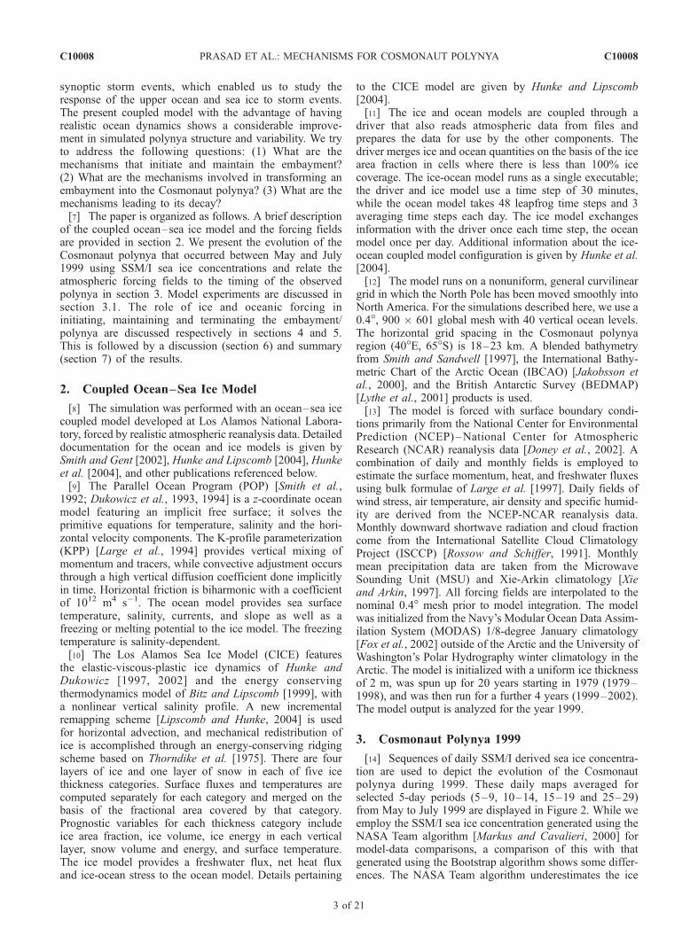
timing of the observed polynya, Figure 3 shows the area-averaged time series of wind speed (m s�1, Figure 3a),zonal and meridional wind stress (N m�2, Figure 3b), andair temperature (�C, Figure 3c) for the period April–July inthe Cosmonaut polynya region (38�–46�E, 63�–66�S, seeFigure 4 for study area). Wind speed plots revealed twoperiods of strong wind events or synoptic storms and theyoccurred respectively during 9–14 June and 29 June to2 July. During these periods the wind speed jumped from4 to �18 m s�1 with generally an easterly-northeasterlydirection. The duration of the first event lasted for 5 dayswhile the second event lasted only for 3 days. Apart from

Figure 2. SSM/I-derived sea ice concentrations (100% = 1) for the Cosmonaut Sea region (Antarctic)showing the Cosmonaut polynya 1999, which is preceded by an embayment during May–July 1999.These maps are averaged for selected 5-day periods, 5–9, 10–14, 15–19, and 25–29.


4 of 21

C10008

these periods, throughout May and June the wind speedwas moderate (�8 m s�1) and the direction was north-easterly. The occurrence of many moderate, but short-lived, wind events are seen throughout the period andthey occurred roughly around 20 April, 2, 4, 10, and 16 May,2, 20, and 25 June, and 23 July. A significant reduction inice concentration (15–19 June, Figure 2) after the passageof the first storm event suggests a relationship betweenthem. From early July, the wind speed showed a graduallydecreasing trend and the wind direction shifted fromnortheast to southwest on 5 July. It is possible that such ashift in the wind direction may have resulted in an advec-tion of ice into the embayment region causing the enclosureof the embayment. However, an examination of the averageair temperature in the polynya region (Figure 3c) indicatesan alternate mechanism leading to its enclosure. A sharpreduction in air temperature from early to middle July mayhave increased the ice growth and subsequent closure of theembayment. Also included in Figure 3c is the downwardlongwave radiative heat flux, which is a function of airtemperature and cloud fraction. Positive longwave heat fluxindicates surface warming. The corresponding longwave

heat flux showed a reduction of 75 W m�2 during thisperiod. In the following sections, we identify the role ofeach forcing mechanism involved in the formation, main-tenance, and decay of the embayment and polynya.

3.1. Model Experiments

3.1.1. Control Run[16] Model derived ice concentrations for the same period

are plotted in Figure 4; these will be compared with theSSM/I data. Superposed is the 10% ice concentrationcontour from the SSM/I data. Outside of the polynya region,the model ice concentration is in good agreement with theSSM/I with differences being under 10%. In the polynyaregion, there is an overall bias in ice concentration by�50%. Except for this bias, the formation of the Cosmo-naut polynya is reasonably well simulated by the model(Figure 4). In particular, the size, shape and time ofoccurrence of the embayment are in approximate agreementwith the SSM/I data (Figure 2). The spatial extent of 10%concentration in SSM/I is in reasonable agreement with themodel’s 60% concentration contour until 10 July. Dailysnapshots showed an almost closed polynya on 10 July,consistent with the SSM/I data. However, an embayment ofreduced ice concentration persisted from mid-July throughearly August, with no evidence for a closed polynya similarto that in the SSM/I observations. From 10–14 Junethrough 15–19 June, significant increases in open waterand embayment area are obvious in both SSM/I and modelconcentrations. The zonal width of the embayment com-puted on the basis of the 60% contour along 65�S was�9.6� (450 km). The average concentration during thisperiod reached the lowest value (40–50%) in the embay-ment followed by a gradual increase in concentration (50–60%). The polynya became completely surrounded byice on 9 July. In the following sections, the result fromthis model run is treated as the control run (CR). While themodel successfully simulated the evolution of the Cosmo-naut polynya in terms of its size, shape and time ofappearance, some discrepancies exist between the modeland SSM/I observations: (1) overall, the simulated con-centration in the polynya region was higher by �50%relative to the SSM/I fields and (2) the closure of thepolynya and its termination after 10 July were not consis-tent with the SSM/I fields.[17] The wind speed will likely have a strong impact on

the temporal and spatial variability of the area of thepolynya and embayment. In addition, the wind speedaffects the sensible and latent heat fluxes at the air–seaice interface, thus the sea ice growth rate. In addition toCR, four perturbation experiments have been performed toexamine the effects of surface winds, surface air temper-ature and sea ice dynamics on the formation and mainte-nance of the Cosmonaut polynya and their details aresummarized in Table 1. Their comparison with the CR willprovide further insight into the mechanisms governing theformation of an embayment and polynya. The first, twoperturbation experiments examine the role of surface windspeed (Experiment 1 (EXP1)) and direction (EXP2). Theirdetails are summarized in Table 1. To explore the effect ofsurface winds on the Cosmonaut polynya, an integration isconducted with a 20% increase of the surface wind speed

Figure 3. Area-averaged (a) wind speed (m s�1), (b) zonal(solid line) and meridional (dotted line) wind stress (N m�2),and (c) surface air temperature (�C, solid line) and down-ward longwave radiative flux (W m�2, dotted line). Thesefields are averaged in the polynya region (38�–46�E, 66�–63�S, see box in Figure 4). The average wind speed betweenApril and July is 7.8 m s�1. There are indications of twostorm events during this period, and they occurred on 9–14 June and 29 June to 2 July 1999.


5 of 21

C10008

(EXP1). The wind speed change is restricted to the region54�W–105�E, 79�S–53�S covering the entire WeddellSea and Cosmonaut Sea regions. Since divergence inthe sea ice has been shown to be well correlated withthe wind field divergence, wind direction would be aninfluencing factor controlling the polynya formation. Toquantify its relationship with the Cosmonaut polynya,EXP2 will be conducted with the sign of the windcomponents reversed. In EXP3, the model is run withthe ice dynamics terms turned off, so that the sea iceexperiences only thermodynamic changes and does notmove. All model simulations are started with January

1999 ocean and ice state taken from CR and integratedthrough a complete year. EXP4 tested the effect of the airtemperature on the closure of the embayment and will bediscussed in section 4.2.3.1.2. Experiment 1[18] The ice concentrations from EXP1, shown in

Figure 5 when the wind speed was increased by 20%,clearly demonstrate the role of surface winds on polynyastructure and maintenance. Except in the Cosmonautpolynya region, the overall ice concentrations showedno significant changes from the control run (CR). In theCosmonaut polynya region, significant reduction in ice

Figure 4. Same as Figure 2, but simulated ice concentration from the control run (CR), in which noforcing fields are altered. Except for the differences in ice concentrations, the size, shape, and time ofappearance of the embayment and polynya are in reasonable agreement with the SSM/I observations.Superposed is the 10% (0.1 ice fractional area) contour from the SSM/I (repeated in Figures 5 and 6). Theocean and ice fields are averaged in the polynya region (38�–46�E, 66�–63�S, see box) and presented inthe following sections.

Table 1. Model Experiments

Parameter Experiment Region Period

NCEP forcing CR global Jan.–Dec. 199920% + wind speed EXP1 54�W to 105�E, 79�–53�S Jan.–Dec. 1999u = �u, v = �v EXP2 54�W to 105�E, 79�–53�S Jan.–Dec. 1999Ice dynamics off EXP3 global Jan.–Dec. 1999Tair(July) ) Tair(June) EXP4 global July 1999


6 of 21

C10008

concentrations occurred, agreeing better with the SSM/Iobservations. An opening of an embayment can be easilyidentified in early May in the Cosmonaut Sea region(38�–46�E, 65�–67�S). A sharp increase in open waterarea occurred on 15–19 June, when the concentrationreached a minimum value of 20% (80% open water).The zonal width of the embayment computed on the basisof 60% contour along 65�S was �14.8� (694 km). Theembayment persisted until the 5–9 July period when itbecame surrounded by ice. The average concentration wasabout 40% when the polynya was formed and it wasapproximately 70% when the Cosmonaut polynya disap-peared. The appearance of a well developed Cosmonautpolynya in the model (5–9 July) occurred approximately5 days earlier than in the SSM/I (10–14 July). A similartime discrepancy was also obvious during the period ofpolynya disappearance. For example, the ice distributionwas nearly uniform during 15–19 July in the Cosmonautpolynya region indicating that the polynya was completelyclosed in contrast to the SSM/I observations, which clearlyshowed a polynya at this time.

3.1.3. Experiment 2[19] In EXP2, the sign of the wind components were

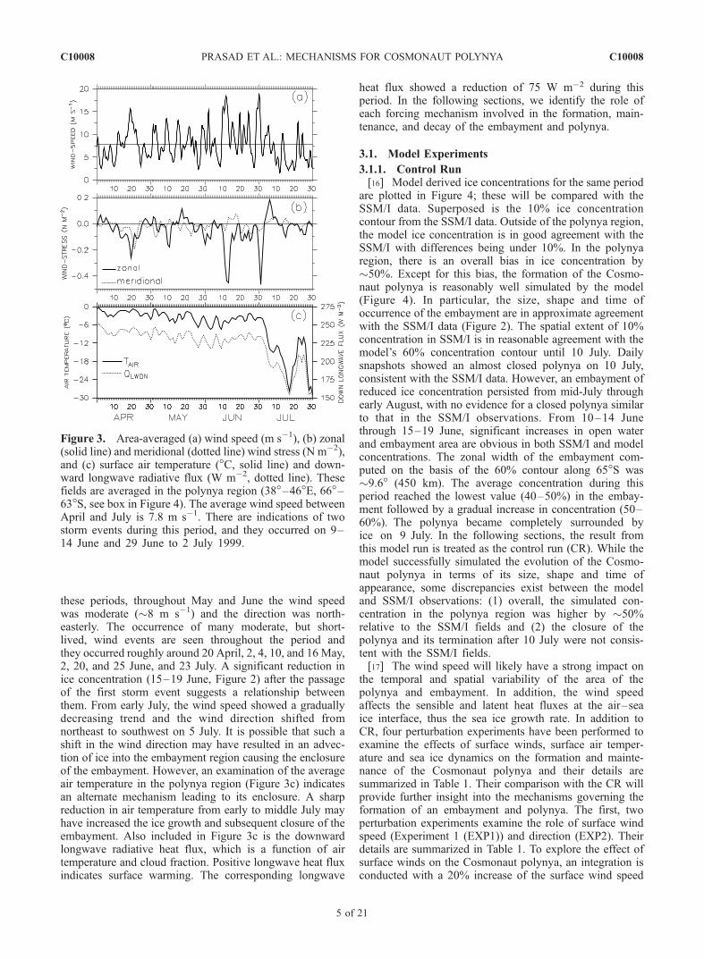
reversed (u = �u, v = �v). The ice concentration from EXP2depicted in Figure 6 clearly revealed that the ice productionand reduction are strongly controlled by the wind direction.The resulting ice concentration did not contain a well-developed embayment and polynya. Overall, the ice con-centration was higher than CR in the Cosmonaut sea region.A conspicuous region of reduced ice concentration huggingthe coast in EXP2 resembled a coastal polynya. Obviously,changes in wind direction affected the polynya formationthrough changes in atmospheric divergence, which drive thesea ice and ocean divergence and hence the oceanic up-welling maintaining the polynya. The impact of changes inwind direction on the dynamics and thermodynamics of thesea ice is discussed in section 4.2.3.1.4. Experiment 3[20] The model is run with the ice dynamics terms

turned off (EXP3), so that the sea ice experiences onlythermodynamic changes and does not move. A comparisonof the sea ice concentration between EXP3 (Figure 6) and

Figure 5. Same as Figure 4, except that it is from model EXP1, in which the wind speed was increasedby 20% from CR. The wind speed change was restricted in the region 54�W to 105�E, 79�–53�Scovering the entire Weddell Sea and Cosmonaut Sea regions. The model integration started in January1999 and was integrated through the polynya period May–July 1999. The increased wind speed led to asignificant reduction in ice concentration, and embayment and polynya structure were greatly improved,agreeing better with SSM/I.


7 of 21

C10008

CR (Figure 4) clearly demonstrates that the sea ice dynamicsare a key determinant of the Cosmonaut polynya. There wasan overall reduction in sea ice concentration in EXP3compared with CR. In contrast to CR, EXP3 failed toreproduce the pattern of polynya formation in July. How-ever, the ice concentration clearly indicated an openingof the embayment from early May, and it persisted until15 May, agreeing better with the SSM/I and EXP1. Whilethe reduced ice concentrations in the Cosmonaut Sea regionsuggest its continued existence, the size and strength of theembayment showed weakening. In particular, a reduction inice concentration and an increase in the embayment areaassociated with the passage of the first storm event (15–19 June) seen in CR were weakened in EXP3. This wasfollowed by a sudden decline in the area of the embayment,eventually leading to its termination earlier than July.

3.2. Open Water Area

[21] We computed the total area of open water andaverage concentrations in the region 38�–46�E, 63�–66�S

from EXP1, EXP2 and EXP3 and compared them with CRin Figure 7a. The SSM/I derived average ice concentrationis shown in Figure 7b. These fields show large differences.The time series plots show a gradual decrease (increase) inopen water area (ice concentration) from early May until10 June, typical for winter conditions. From 10 June tomid-July, the open water area increased significantly inEXP1 in comparison with CR. For example, when the firststorm event peaked on 15 June, the open water areajumped from 53 � 103 km2 (12 June) to 88 � 103 km2

(20 June) yielding 35 � 103 km2 in 8 days in EXP1, whileit was only 21 � 103 km2 in CR. In response to the firststorm event, both SSM/I and CR ice concentration showeda 15% reduction. The SSM/I concentration began toincrease abruptly from early July 1999 at a rate of3.4% d�1, indicating the termination of the Cosmonautpolynya. From 15 July onward, the average EXP1 concen-tration (and area of open water) was identical to the CR,which suggests that wind speed has negligible effect on thesea ice growth rate during this period. A second peak of

Figure 6. Same as Figure 4, but from EXP2 (top two rows) and EXP3 (bottom two rows). EXP2 is runwith the sign of the wind components reversed (u = �u, v = �v), and EXP3 is run with the ice dynamics(elastic-viscous-plastic) [Hunke and Dukowicz, 1997] turned off. For clarity, only selected periods areshown. The importance of ice dynamics is obvious from June in EXP3, when the embayment began toweaken significantly, which eventually caused its termination. EXP2 failed to contain an embayment andpolynya, which demonstrates that ice convergence-divergence are the key processes determining theevolution of the embayment/polynya.


8 of 21

C10008

open water area that occurred in response to the secondstorm event in EXP1 was less pronounced in CR.

4. Sea Ice Fluxes

4.1. Sea Surface Temperature, Heat, and FreshwaterFluxes

[22] An important aspect of the Cosmonaut polynya 1999was that the region remained ice-free for several weeksbeginning in early May while ice continued to grow in theadjacent regions (Figure 2). We can envisage such acondition occurring via (1) upward oceanic heat flux,(2) advection of ice away from the formation region bythe action of surface wind or ocean currents, (3) upwell-ing and mixing associated with the passage of synopticstorms, and/or (4) a combination of two or more of theseprocesses.[23] Time series of sea surface temperature (SST)

(Figure 8a), fluxes of heat (Figure 8b) and freshwater(Figure 8c) from the four model runs (CR, EXP1, EXP2and EXP3) are presented in Figure 8. These fields areaveraged for the polynya region (38�–46�E, 63�–66�S).Overall, the SST showed a gradual decrease from earlyMay to 25 May, and it then remained close to a near-freezing (�1.75�C) condition until 10 June. Thereafter, theSST rose quickly to �1.6�C and fell back to �1.75�C on20 June. A similar event also occurred between 30 Juneand 10 July. These two events are clearly associated withthe passage of synoptic storms. The wind stress presentedin Figure 3 confirms the occurrence of such events. Thusthe upwelling and mixing are the likely mechanismsleading to the warm SST during the periods of strong

winds. This is further elucidated in section 5.3. The seasurface salinity (SSS, psu) from CR (Figure 8c) progres-sively increased at a rate of 5.4 � 10�3 psu d�1 during theentire period. A small drop in SSS by 0.03 psu occurredduring the storm periods. Also evident in Figure 8a areintermittent periods of somewhat mild SST warmingduring May, which is more pronounced in EXP1 butabsent in EXP2. Both EXP1 and EXP3 generated higherSSTs in early May, causing the opening of an embayment.However, a lack of increase in SST during the stormevents prematurely terminated the embayment in EXP3.[24] The time series of net heat flux (W m�2) across the

ice-ocean interface (from the ice model) for the Cosmo-naut polynya region is displayed in Figure 8b. Positive(negative) values indicate heat flux from the ice (ocean) tothe ocean (ice). A substantial jump in heat flux from theocean to the ice occurred during the period of strongwinds, which is consistent with the SST. The first eventgenerated a heat flux of �85 W m�2 into the ice while thesecond produced a flux of �60 W m�2. The bursts ofupward heat flux promoted enhanced ice melting andinhibited further ice growth in the embayment region. Therelease of freshwater into the ocean due to melted ice isillustrated in Figure 8c. There is 2 cm d�1 freshwater flux

Figure 7. Area-averaged (a) open water area (km2) and(b) average ice concentration in the polynya region (38�–46�E, 66�–63�S) for the time period May–July 1999 frommodel simulations CR (solid lines), EXP1 (dotted lines),EXP2 (dashed lines), EXP3 (dash-dotted lines), and SSM/I(dash-dot-dotted lines). The correlations between theSSM/I sea ice concentrations and the model experimentsCR, EXP1, EXP2, and EXP3 are 0.60, 0.75, 0.72, and0.65, respectively.

Figure 8. Area-averaged (a) SST (�C), (b) heat flux(W m�2), and (c) freshwater flux (cm d�1) in the polynyaarea (38�–46�E, 66�–63�S) from model runs CR (solidlines), EXP1 (dotted lines), EXP2 (dashed lines), and EXP3(dash-dotted lines). Also included in Figure 8c is the seasurface salinity (SSS, psu) from CR. Positive valuesindicate downward fluxes of heat and freshwater from theice to the ocean. CR and EXP1 show enhanced fluxes ofheat and freshwater across the ice-ocean interface and SSTincrease during the period of storm events while EXP2 andEXP3 show no burst of fluxes and SST.


9 of 21

C10008

into the ocean during the period of the first storm event.This freshwater input in turn stabilized the water column byincreasing the stratification. Throughout the period, EXP2and EXP3 heat flux remained under 25 W m�2, which is inagreement with CR and EXP1 except during the stormperiods. The impact of increased wind speed (EXP1) wasevident only during the strong wind conditions although thepattern of SST between CR and EXP1 was not the same.Although the wind stress magnitude was the same in bothCR and EXP2, the wind direction altered the ice/oceandivergence and hence the upward heat flux. The windreversal in EXP2 lead to dramatic changes in heat fluxbecause of oceanic downwelling, which is discussed insection 5.3. Except during the storms, a net loss of fresh-water flux by the ocean via ice formation increased the SSSprogressively. What is clear from this analysis is that thesignificant reduction in ice concentration and increase inthe embayment area that occurred during 15–19 June(Figure 4) was primarily driven by the upward heat fluxand associated SST warming. The impact of the secondevent on the embayment area, however, was somewhatmitigated by the reversal of the ice drift and larger air-seatemperature differences, which aided rapid ice growth (seesections 4.2 and 4.4).[25] Clearly, the exchange of heat between the ocean and

ice plays a vital role in the maintenance of the embayment,particularly those associated with the storms, which canprovide ample upward heat flux to keep the region ice-freefor several weeks. Inclusion of such realistic oceanic heatflux (which is often prescribed as a spatially uniform heatflux) in the future coupled atmosphere–sea ice modelswould certainly improve the polynya simulation. Parkinson[1983] specified a spatially uniform 25 W m�2 ocean heatflux for the simulation of the Weddell polynya. This valueagrees with our estimate except during the strong windconditions. In an attempt to simulate the Cosmonautpolynya that occurred on 6–8 August 1988, Bailey et al.[2004], using a coupled atmosphere–sea ice model, per-formed several numerical experiments with vertical oceanheat flux values varying from 15 W m�2 to 200 W m�2.They noted a sharp reduction in ice concentration in thepolynya region when the heat flux was set uniformly to15 W m�2, except for a patch of 200 W m�2 centeredwithin the polynya region. This extreme heat flux can beattained under the action of strong winds; for example,during the Antarctic Zone Flux Experiment (ANZFLUX)in July and August 1994, upward heat fluxes exceeding100 W m�2 were observed in the eastern Weddell Sea[McPhee et al., 1996]. Thus the significant contributionof heat flux induced by the storms should be representedaccurately in coupled atmosphere–sea ice models, ratherthan by a spatially uniform constant value.

4.2. Ice Growth and Melting

[26] There are number of factors that influence icegrowth/melt processes such as oceanic heat flux, ice driftand deformation, wind, and air temperature. Time series ofarea-averaged congelation (Figure 9a), frazil (Figure 9b) icegrowth rates, and basal ice melt (Figure 9c) from CR,EXP1, EXP2 and EXP3 are plotted in Figures 9. Thesefields represent the average growth/melt rate per unit icearea. The congelation ice growth occurs thermodynamically

by freezing onto an existing ice bottom. It should be notedthat the bias in the ice concentration within the polynyaaffects the relative importance of frazil and congelation icegrowth in the simulation because frazil forms in open water,while congelation ice forms at the base of the existing ice.The rate of congelation ice growth is much larger than thefrazil ice growth during the entire period. The occurrence ofstrong winds on 10–15 June and 1–5 July were charac-terized by a prolonged period (�5 days) of no ice growth.The former period was followed by a rapid increase inembayment area on 15–19 June (Figure 4) while the latterevent had little influence on the embayment area. It wasduring these periods that the highest rate of basal icemelting (2.5 cm d�1) occurred in the Cosmonaut Searegion (Figure 9c). This suggests that even small changesin ocean temperature (�0.2�C, Figure 8a) can have sig-nificant impacts on the basal melt rate. During the firstevent, a heat flux of �85 W m�2 (Figure 8b) from theocean to ice yielded a basal melt rate of 2.5 cm d�1.[27] The closure of the embayment began on 5 July, when

the congelation ice growth at the bottom of the existing iceincreased rapidly. The congelation ice growth jumped froma zero value on 5 July to 1.1 cm d�1 on 17 July. Thisoccurred during a period of southwesterly winds, when theice had a net northeasterly drift to the northwestern side ofthe embayment. Also there was a close relationship betweenair temperature (Figure 3c) and the congelation ice growthfrom 5 July to late July. Thus the southwesterly winds inthis region not only caused the ice to drift northwest but alsocarried very cold continental air. The embayment rapidlyrefreezes because of the enormous temperature differencebetween the atmosphere (�25�C) and the ocean (�1.8�C).[28] From late May to early July, the congelation ice

growth in EXP1 and EXP2 remained quite similar. EXP1formed more frazil ice because of greater open water areas(allowing greater ocean cooling), while congelation icegrowth depended on both the ocean temperature and theexisting ice cover. Since these are fairly similar in CR andEXP1, the congelation growth rates are similar. Centered onmid-May, EXP1 revealed slower congelation ice growththan CR and EXP2. Basal melting rates during the periodsof strong winds differed significantly; EXP1 produced thehighest melting rate (>4.5 cm d�1) while EXP2 and EXP3yielded <0.5 cm d�1 owing to the differences in SST and netheat flux from the ocean to the ice (Figure 8) among thefour model runs.[29] Although the rapid congelation ice growth during

July correlated well with the air temperature, it is unclearwhether the rapid decline of air temperature accelerated theclosure of the embayment and the subsequent formation ofthe polynya. To address this issue, we performed anadditional model experiment (EXP4) in which the July airtemperature was replaced with that from June therebyeliminating the sharp drop in air temperature so that themodel was run for July 1999 (with June 1999 air temper-ature). The air temperature used in EXP4 and CR and thecorresponding congelation ice growth are plotted inFigure 9d. The apparent reduction of congelation ice growthrate in EXP4 from CR clearly demonstrated that the airtemperature was partly accountable for the rapid growthseen in CR. The sea ice concentrations from EXP4 (figurenot presented) suggest that differences in air temperature


10 of 21

C10008

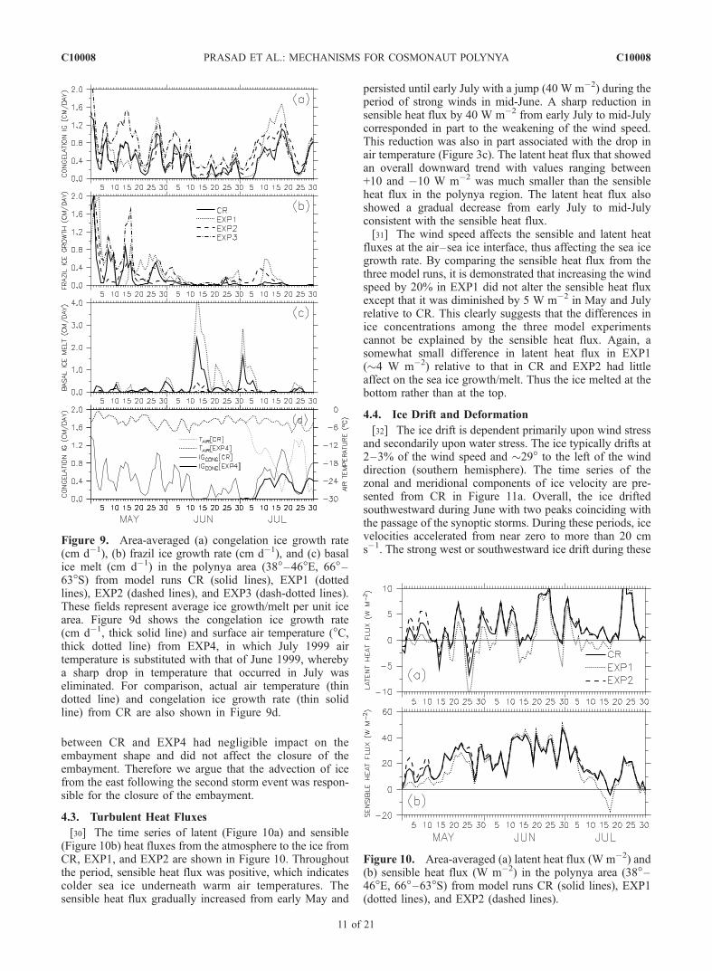
between CR and EXP4 had negligible impact on theembayment shape and did not affect the closure of theembayment. Therefore we argue that the advection of icefrom the east following the second storm event was respon-sible for the closure of the embayment.

4.3. Turbulent Heat Fluxes

[30] The time series of latent (Figure 10a) and sensible(Figure 10b) heat fluxes from the atmosphere to the ice fromCR, EXP1, and EXP2 are shown in Figure 10. Throughoutthe period, sensible heat flux was positive, which indicatescolder sea ice underneath warm air temperatures. Thesensible heat flux gradually increased from early May and

persisted until early July with a jump (40 W m�2) during theperiod of strong winds in mid-June. A sharp reduction insensible heat flux by 40 W m�2 from early July to mid-Julycorresponded in part to the weakening of the wind speed.This reduction was also in part associated with the drop inair temperature (Figure 3c). The latent heat flux that showedan overall downward trend with values ranging between+10 and �10 W m�2 was much smaller than the sensibleheat flux in the polynya region. The latent heat flux alsoshowed a gradual decrease from early July to mid-Julyconsistent with the sensible heat flux.[31] The wind speed affects the sensible and latent heat

fluxes at the air–sea ice interface, thus affecting the sea icegrowth rate. By comparing the sensible heat flux from thethree model runs, it is demonstrated that increasing the windspeed by 20% in EXP1 did not alter the sensible heat fluxexcept that it was diminished by 5 W m�2 in May and Julyrelative to CR. This clearly suggests that the differences inice concentrations among the three model experimentscannot be explained by the sensible heat flux. Again, asomewhat small difference in latent heat flux in EXP1(�4 W m�2) relative to that in CR and EXP2 had littleaffect on the sea ice growth/melt. Thus the ice melted at thebottom rather than at the top.

4.4. Ice Drift and Deformation

[32] The ice drift is dependent primarily upon wind stressand secondarily upon water stress. The ice typically drifts at2–3% of the wind speed and �29� to the left of the winddirection (southern hemisphere). The time series of thezonal and meridional components of ice velocity are pre-sented from CR in Figure 11a. Overall, the ice driftedsouthwestward during June with two peaks coinciding withthe passage of the synoptic storms. During these periods, icevelocities accelerated from near zero to more than 20 cms�1. The strong west or southwestward ice drift during these

Figure 9. Area-averaged (a) congelation ice growth rate(cm d�1), (b) frazil ice growth rate (cm d�1), and (c) basalice melt (cm d�1) in the polynya area (38�–46�E, 66�–63�S) from model runs CR (solid lines), EXP1 (dottedlines), EXP2 (dashed lines), and EXP3 (dash-dotted lines).These fields represent average ice growth/melt per unit icearea. Figure 9d shows the congelation ice growth rate(cm d�1, thick solid line) and surface air temperature (�C,thick dotted line) from EXP4, in which July 1999 airtemperature is substituted with that of June 1999, wherebya sharp drop in temperature that occurred in July waseliminated. For comparison, actual air temperature (thindotted line) and congelation ice growth rate (thin solidline) from CR are also shown in Figure 9d.

Figure 10. Area-averaged (a) latent heat flux (W m�2) and(b) sensible heat flux (W m�2) in the polynya area (38�–46�E, 66�–63�S) from model runs CR (solid lines), EXP1(dotted lines), and EXP2 (dashed lines).


11 of 21

C10008

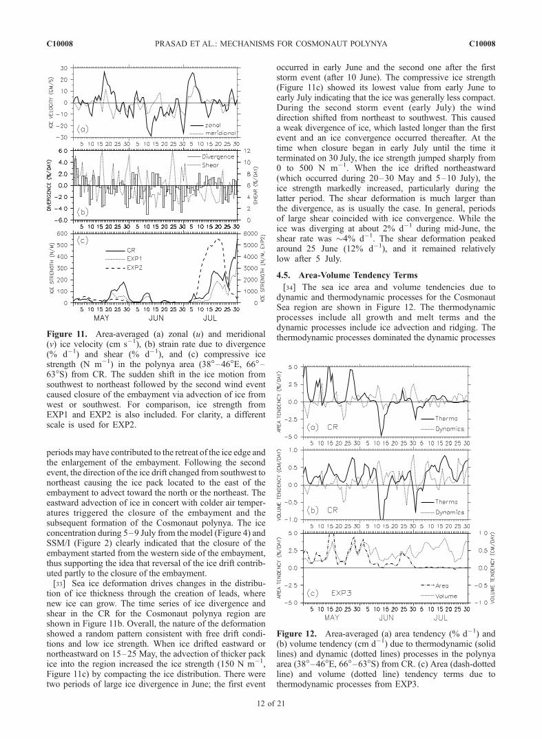
periods may have contributed to the retreat of the ice edge andthe enlargement of the embayment. Following the secondevent, the direction of the ice drift changed from southwest tonortheast causing the ice pack located to the east of theembayment to advect toward the north or the northeast. Theeastward advection of ice in concert with colder air temper-atures triggered the closure of the embayment and thesubsequent formation of the Cosmonaut polynya. The iceconcentration during 5–9 July from the model (Figure 4) andSSM/I (Figure 2) clearly indicated that the closure of theembayment started from the western side of the embayment,thus supporting the idea that reversal of the ice drift contrib-uted partly to the closure of the embayment.[33] Sea ice deformation drives changes in the distribu-

tion of ice thickness through the creation of leads, wherenew ice can grow. The time series of ice divergence andshear in the CR for the Cosmonaut polynya region areshown in Figure 11b. Overall, the nature of the deformationshowed a random pattern consistent with free drift condi-tions and low ice strength. When ice drifted eastward ornortheastward on 15–25 May, the advection of thicker packice into the region increased the ice strength (150 N m�1,Figure 11c) by compacting the ice distribution. There weretwo periods of large ice divergence in June; the first event

occurred in early June and the second one after the firststorm event (after 10 June). The compressive ice strength(Figure 11c) showed its lowest value from early June toearly July indicating that the ice was generally less compact.During the second storm event (early July) the winddirection shifted from northeast to southwest. This causeda weak divergence of ice, which lasted longer than the firstevent and an ice convergence occurred thereafter. At thetime when closure began in early July until the time itterminated on 30 July, the ice strength jumped sharply from0 to 500 N m�1. When the ice drifted northeastward(which occurred during 20–30 May and 5–10 July), theice strength markedly increased, particularly during thelatter period. The shear deformation is much larger thanthe divergence, as is usually the case. In general, periodsof large shear coincided with ice convergence. While theice was diverging at about 2% d�1 during mid-June, theshear rate was �4% d�1. The shear deformation peakedaround 25 June (12% d�1), and it remained relativelylow after 5 July.

4.5. Area-Volume Tendency Terms

[34] The sea ice area and volume tendencies due todynamic and thermodynamic processes for the CosmonautSea region are shown in Figure 12. The thermodynamicprocesses include all growth and melt terms and thedynamic processes include ice advection and ridging. Thethermodynamic processes dominated the dynamic processesFigure 11. Area-averaged (a) zonal (u) and meridional

(v) ice velocity (cm s�1), (b) strain rate due to divergence(% d�1) and shear (% d�1), and (c) compressive icestrength (N m�1) in the polynya area (38�–46�E, 66�–63�S) from CR. The sudden shift in the ice motion fromsouthwest to northeast followed by the second wind eventcaused closure of the embayment via advection of ice fromwest or southwest. For comparison, ice strength fromEXP1 and EXP2 is also included. For clarity, a differentscale is used for EXP2.

Figure 12. Area-averaged (a) area tendency (% d�1) and(b) volume tendency (cm d�1) due to thermodynamic (solidlines) and dynamic (dotted lines) processes in the polynyaarea (38�–46�E, 66�–63�S) from CR. (c) Area (dash-dottedline) and volume (dotted line) tendency terms due tothermodynamic processes from EXP3.


12 of 21

C10008

for both area and volume tendency terms. Except during theperiod of storm events, the ice area and volume showed anoverall increase primarily due to the thermodynamic pro-cesses. A significant reduction in the area and volume of iceduring the storm periods was driven by the thermodynamicprocesses, which is consistent with ice/ocean heat flux andSST. There were three periods in May (5, 11, and 21 May)during which the thermodynamic contribution to the areafell to a near-zero value. The SST (and heat flux) duringthese periods clearly showed a mild jump (Figures 8aand 8b) although it was much weaker than that associatedwith the storm events. However, such contributions couldprovide sufficient heat to prevent ice formation in theregion. It is interesting to note that the dynamic andthermodynamic contributions are of equal magnitude butopposite sign around the second event. This led to littlechange in the ice concentration. After the closure of theembayment on 5 July, both dynamic and thermodynamicprocesses appeared to have less impact on the ice areawhile their contributions to the volume increase weresignificant. This is consistent with the increased rate ofcongelation ice growth, which is driven by the colder airtemperatures. Thus the large air-sea temperature differencetogether with dynamic processes via the advection of iceby the ocean currents or winds on 5–10 July led to theclosure of the embayment. The volume and area changedue to thermodynamic processes from EXP3 are depictedin Figure 12c. By comparing these fields between CR andEXP3, it is demonstrated that the sea ice dynamics playan important role in the maintenance of the embayment. Inthe absence of ice dynamics, the decreasing ice area and

volume due to thermodynamic processes as a consequenceof the storm events, did not take place.

5. Role of Oceanic Forcing

[35] In the preceding sections, we discussed the roleof ice forcing on the initiation and maintenance of theCosmonaut polynya that occurred during May–July 1999.While the model results are strongly suggestive of theinfluence of the winds on the occurrence of the Cosmonautpolynya, it may also be influenced by the atmospheric(synoptic) forced local oceanic responses through Ekmandivergence or mixing. An important aspect of the eddypotential vorticity argument of Comiso and Gordon [1996]is that eddies that shed from instabilities in the AntarcticDivergence could become a source of heat because ofupwelling or local divergence. This contribution, however,cannot be addressed with an eddy-permitting model. Comisoand Gordon [1996] suggested that the heat provided fromthe upwelled circumpolar deep water was sufficient tomaintain an ice-free region in the ECP. The increased inputof heat from beneath the mixed layer during storm mixingcan be substantial in polynya intensification processes.For example, a significant increase in the embayment area(and decrease in ice concentration) occurred after the firststorm event (10–14 June, Figure 4). It is, however,unclear what mechanisms kept this region ice-free andprevented it from closing and freezing for a prolongedperiod of time. Therefore characterizing the role ofoceanic setup is important for understanding the evolutionof the embayment and the Cosmonaut polynya.[36] In the following sections, we attempt to address

(1) the preconditioning that leads to the formation of theembayment, (2) divergence of ocean currents and upwelling,and (3) wind-driven mixing associated with the passage ofsynoptic storms. Since SSM/I and model ice concentrationalready showed an opening of the embayment on 1 May, itis implied that the first appearance of the embayment canbe traced back to April. So in the following sections, thefocus will be placed on the period April through Julyrather than May–July.

5.1. Ocean Currents

[37] Although the dominant driving force on the sea ice isthe wind, ice can also undergo small changes because of theocean currents. The area-averaged ocean surface currents(5 m) in the polynya region are displayed in Figure 13aduring April–July 1999. Surface velocity in the south-westerly direction (>10 cm s�1) during the storm eventssupports the idea that the sea ice was being advected awayfrom the embayment region. The southeast advection ofsea ice driven by strong northeasterly winds (Figure 3b)on 16–26 April may have opened the leads that wereenlarged by subsequent melting due to upward heat flux.It is during this period that the embayment made its firstappearance. The northeast flowing currents following thesecond storm event caused the closure of the embaymentvia ice advection into the region. A similar, but ratherweak and short-lived, advection event that took place on10–15 May, however, did not cause the closure of theembayment. The embayment may have lasted for severalweeks partly because of (1) the constant movement of the

Figure 13. Area-averaged (a) zonal (solid line) andmeridional (dotted line) ocean surface currents (5 m, cm s�1)and (b) net heat flux (W m�2, solid line), sensible heatflux (W m�2, dotted line), surface heat due to ice melt(W m�2, dash-dotted line), and longwave heat flux (W m�2,dash-dot-dotted line) from the ocean model (CR) in thepolynya area (38�–46�E, 66�–63�S) during April–July1999. Negative values of net heat flux indicate the loss ofheat from the ocean to the atmosphere.


13 of 21

C10008

newly formed ice by ocean currents before they couldform continuous ice cover, (2) the upward heat fluxfollowing the passage of storms, and (3) a combinationof both processes.[38] The question remains, what ocean currents accom-

plish this removal of ice from the embayment region? Webegan to answer this by investigating the spatial pattern ofocean surface currents from CR, which is depicted inFigure 14 for 24 April, 13 June, 2 July, and 10 July.Throughout the period, an eastward flowing AntarcticCircumpolar Current (ACC) north of �64�S dominatesthe surface circulation. In the Cape Ann region (between50� and 60�E), part of the eastward flowing ACC turnssouth roughly at 60�S, 50�E (Figures 14b and 14c). As thewater approaches Antarctica, it joins a west-southwestwardflowing Antarctic coastal current. The mean speed of the

coastal current was �20 cm s�1. These two opposingcoastal and offshore currents are separated by the AntarcticDivergence at around 65�S. An interesting aspect of thiscoastal current is its large seasonality coincident with theembayment/polynya life cycle. From early April to lateJune, as the embayment was growing and strengthening, thecoastal current to the southeast of the embayment flowedsouthwestward with its maximum strength occurring duringthe storm events. Following the second storm event, thecoastal current weakened significantly and by 10 July thecurrent reversed and became northeastward.[39] The generally east-northeasterly winds in this region

induce a south-southwestward ice drift and carry relativelywarm moist air from the open ocean. The sea ice iscontinually removed southwestward from the embaymentregion owing to the action of prevailing winds and ocean

Figure 14. Daily average surface ocean currents (cm s�1) for (a) 24 April (b), 13 June, (c) 2 July, and(d) 10 July 1999 from CR. Shaded regions indicate SSM/I-derived sea ice concentrations during 30 April(Figure 14a), 15 June (Figure 14b), 5 July (Figure 14c), and 10 July 1999 (Figure 14d). An eastwardflowing Antarctic Circumpolar Current (ACC) to the north of the Antarctic Convergence (65�S) and asouthwestward flowing coastal current to the south are evident. The coastal current keeps the embaymentopen via advection of ice southwestward (Figures 14a–14c), and reversal of the coastal current triggeredthe closure of the embayment (Figure 14d).


14 of 21

C10008

currents. The rate of ice transport by the coastal currentexceeds the relatively slow ice growth. To the northwest ofthe embayment, the eastward advection of ice into theembayment region was restricted because of the weaksurface currents. Thus the embayment remained open forseveral weeks partly because of the divergence of ice by thecoastal currents coincident with weak ice growth. Anoverall reduction in wind speed in the coastal region fromearly July weakened the coastal currents and ice divergence.At the same time, a dramatic reversal of the winds fromnortheast to southwest advected ice eastward into theembayment region. This, coincident with the large temper-ature difference between the ocean and atmosphere resultedin the closure of the embayment.[40] The role of coastal currents in initiating and main-

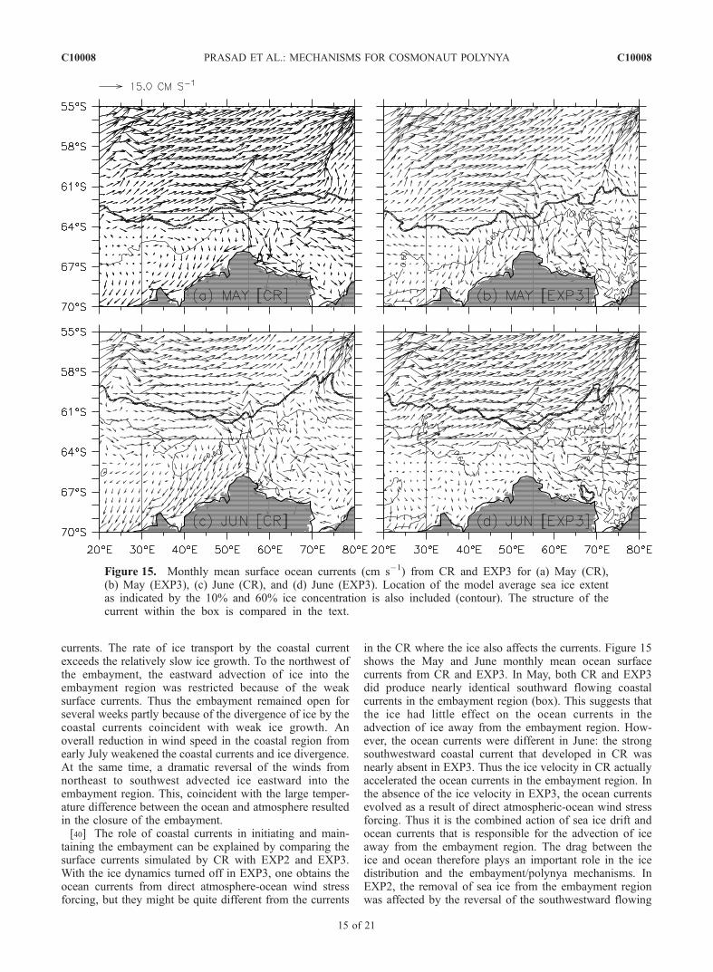
taining the embayment can be explained by comparing thesurface currents simulated by CR with EXP2 and EXP3.With the ice dynamics turned off in EXP3, one obtains theocean currents from direct atmosphere-ocean wind stressforcing, but they might be quite different from the currents

in the CR where the ice also affects the currents. Figure 15shows the May and June monthly mean ocean surfacecurrents from CR and EXP3. In May, both CR and EXP3did produce nearly identical southward flowing coastalcurrents in the embayment region (box). This suggests thatthe ice had little effect on the ocean currents in theadvection of ice away from the embayment region. How-ever, the ocean currents were different in June: the strongsouthwestward coastal current that developed in CR wasnearly absent in EXP3. Thus the ice velocity in CR actuallyaccelerated the ocean currents in the embayment region. Inthe absence of the ice velocity in EXP3, the ocean currentsevolved as a result of direct atmospheric-ocean wind stressforcing. Thus it is the combined action of sea ice drift andocean currents that is responsible for the advection of iceaway from the embayment region. The drag between theice and ocean therefore plays an important role in the icedistribution and the embayment/polynya mechanisms. InEXP2, the removal of sea ice from the embayment regionwas affected by the reversal of the southwestward flowing

Figure 15. Monthly mean surface ocean currents (cm s�1) from CR and EXP3 for (a) May (CR),(b) May (EXP3), (c) June (CR), and (d) June (EXP3). Location of the model average sea ice extentas indicated by the 10% and 60% ice concentration is also included (contour). The structure of thecurrent within the box is compared in the text.


15 of 21

C10008

coastal currents (figures not shown). In contrast to CR, thenortheastward coastal currents in EXP2 advected ice intorather than out of the embayment region thereby preventingthe embayment from opening. The continued movement ofice away from the coast by the northeastward coastalcurrents in EXP2 opened an ice-free region along the coastof Antarctica (Figure 6).

5.2. Heat Fluxes

[41] Upward heat transfer can occur through verticalmixing of heat from deeper water or through upwardadvection of heat by such mechanisms as wind-drivenupwelling, making sufficient oceanic heat available to erodethe underside of the ice cover. Once open, the polynya willrapidly lose heat to the atmosphere but the source of warmerwater may be sufficient to prevent freezing. If not, theoriginal advective currents may carry away newly formedice crystals before they can form continuous ice cover. Thetime series of net heat flux (NHF, W m�2), sensible heatflux (SHF, W m�2), surface melt heat flux (SMHF, W m�2)and longwave heat flux (LWF, W m�2) averaged for thepolynya region (38�–46�E, 66�–63�S) from the oceanmodel are shown in Figure 13b. Except during stormperiods, the exchange of heat between the ocean andatmosphere differs from that between the ocean and the

ice (compare Figures 8b and 13b). This difference is largelydue to the longwave heat flux. Local changes in wind speed,particularly those associated with the passage of synopticstorm events, caused a rapid loss of heat to the atmospherefrom 25 to 100 W m�2 within a few days. It is remarkablethat this peak value of heat loss at the height of the firststorm event (100 W m�2) in June was comparable withthat during 20 April, when the entire region was mostlyice-free. From mid-April to 7 June, as the ice was formingin the embayment, the heat loss to the atmospheredecreased gradually. The sensible heat flux, which wasunder 10 W m�2 prior to the embayment closure (5 July),was not a significant contributor to the net heat flux. Thesurface heat flux due to ice melt jumped from 10 to morethan 50 W m�2 during the passage of the storms.

5.3. Upwelling and Mixing

[42] What might be the mechanisms responsible for theincreased oceanic heat flux during the storm events? Weargue that with the impetus provided by the storm and theresulting wind-driven vertical mixing increase the heat inputfrom beneath the mixed layer. To demonstrate this, weexamine the vertical displacement of the �1.6�C isothermdepth (D�1.6) prior to, during, and after each of the twostorms discussed earlier. We have chosen this isotherm

Figure 16. Sequences of selected isotherm depths along 65�S during (a) 11–18 June, (b) 1–9 July,(c) 20 April to 15 May, and (d) 1 April to 30 July 1999 from CR. Figures 16a–16c show the verticaldisplacement of �1.6�C isotherm depth associated with the strong wind events, and Figure 16d showsthe 0�C isotherm depth. The upward lifting of the �1.6�C isotherm from 30 m depth to the surfaceoccurred at the time of storm events.


16 of 21

C10008

because it best represents the vertical mixing owing to itsproximity to the surface through outcropping into thesurface mixed layer. The sequences of D�1.6 along 65�Sfor the two storm periods are depicted in Figures 16aand 16b, respectively. Prior to the first event (10–16 June1999, Figure 16a), on 11 and 12 June, D�1.6 waslocated at 27 m in the Cosmonaut polynya region. Theisotherm outcropping into the surface layer occurredduring 13–15 June, that is, between 12 and 13 June,the isotherm was displaced vertically by 25 m. By18 June, D�1.6 had returned to its original position of27 m where it was located prior to the event. During thesecond event (1–9 July 1999), the location of D�1.6

remained close to 27 m prior to the event with anexception that its position slightly deepened in the easternhalf of the polynya region. As the storm was strengthen-ing, the isotherm continued its upward displacement untilit reached the surface by 3–4 July. On 8 July the isothermreturned to the original depth of 30 m. The region thatexperienced near-surface warming due to the action ofstrong winds extended zonally from 38� to 46�E, roughly376 km.[43] Clearly, the storm-induced oceanic upward heat flux

and warmer SST (Figures 16a and 16b) provided sufficientheat to erode the underside of the ice cover and contributedto the strengthening of the Cosmonaut polynya. However,the presence of warmer water in this region can be seenduring the nonstorm periods beginning in early April.Sequences of D�1.6 plotted in Figure 16c for April–Mayclearly demonstrate this. Between 35� and 45�E, thepresence of warmer water, as evidenced by the surfacingof D�1.6 from early April to 8 May, was sufficient toprevent freezing and/or delay ice formation while icegrowth continued in the surrounding regions. The exis-tence of this warmer water in the Cosmonaut Sea led topreconditioning for the embayment formation.[44] If the thermocline is sufficiently shallow, upward

heat transfer can occur through vertical mixing (primarilywind-driven) of heat from deeper water or throughupward advection of heat by wind-driven upwelling. Toexamine the nature of the thermocline variability in theCosmonaut Sea region, we show sequences of the 0�Cisotherm depth from early April to late July 1999 inFigure 16d. The shoaling of the thermocline by more than60 m between 35� and 45�E from adjacent regionsindicates upwelling. Throughout the period, as the winterseason progressed, the depth of the thermocline was gradu-ally deepening, except during the periods of strong winds.For example, the isotherm deepened from 20 to 55 mbetween April and July. Surface warming can occur onlywhen conditions are favorable for near-surface mixing.During April, when the thermocline was sufficiently shallow(20 m), winds with moderate speeds were able to verticallymix the water column so that the region remained warmer.On the other hand, when the thermocline was relativelydeeper in June, more energy was required for mixing thewater column.[45] The thermocline depth, upwelling and upward heat

flux through vertical mixing are closely related, so bothatmospheric and oceanic forcing effects can be substantialin the processes governing the lifecycle of polynyas in theCosmonaut Sea. Therefore it is expected that any changes in

the atmospheric forcing would have a significant effect onthe thermal fields and hence the oceanic upwelling thatmaintains the polynya. A comparison of the upper oceanthermal fields and vertical velocity from the three modelexperiments provided further insights regarding the polynyamechanisms. The vertical distribution of the temperature(upper 150 m) from CR, EXP1, EXP2 and EXP3 for Apriland June 1999 (Figure 17 (top)) shows interesting changesin the thermocline pattern. The corresponding verticalvelocity (m d�1) for June 1999 is depicted in Figure 17(bottom). West of 45�E, both CR and EXP1 indicatedupwelling of warm water at a rate of >0.2 m d�1 (>2.3 �10�4 cm s�1), which agrees with the ECP upwelling rate of2.6 � 10�4 cm s�1 [Comiso and Gordon, 1996]. Theshoaling of the thermocline due to oceanic upwellingpreconditioned the surface for embayment formation. Whenthe wind speed was increased by 20% (EXP1), warm waterupwelling (�1 m d�1) and hence the SST (�35�–45�E)somewhat increased. The mixed layer depth during Aprilwas �20 m on the basis of 0.5�C temperature gradientcriterion, and it deepened to �40 m in June (CR and EXP1).Thus stronger kinetic-energy-driven mixing owing to in-creased wind speed coincident with stronger upwelling ledto higher SSTs, which caused significant reduction in iceconcentration. When the wind components were reversed(EXP2), the region experienced oceanic downwelling(instead of upwelling), which in turn yielded relativelycolder SSTs in the Cosmonaut Sea (�35�–45�E) duringApril. Further depression of the thermocline (induced bydownwelling) during June in this region coincident with adeep mixed layer (>60 m) inhibited the upward heat fluxthrough vertical mixing.[46] While the downwelling mechanism can be used to

explain the absence of large upward heat fluxes during thestorm wind events in EXP2 (Figure 8), obviously the samemechanism is not applicable for that in EXP3. The upperocean thermal structure and upwelling are not likely to beaffected by the absence of ice dynamics in EXP3. Toexamine this, we show vertical sections of temperatureand vertical velocity from EXP3 during June 1999 inFigure 17. As expected, no significant changes are evidentin the upwelling intensity or the location of the mixedlayer depth compared to CR. Thus the upward heat fluxdifferences between EXP3 and CR during the periods ofstrong winds are not caused by the upwelling. Rather, itis the difference in wind-driven vertical mixing that isresponsible for the large heat flux differences. Lack of icemovement in EXP3 prevented the upward heat fluxthrough leads opened by ice advection and verticalmixing. In principle, the ocean model computes all theterms (advective and diffusive as well as horizontal andvertical differences); but they are not saved for lateranalysis.

6. Discussion

[47] Employing results from a 0.4� fully global, coupledocean-ice model we investigated the physical processesresponsible for the initiation, maintenance and terminationof the Cosmonaut polynya with a focus on the recent 1999polynya. In this particular year, the Cosmonaut polynyafirst appeared on 25–30 April 1999 in the form of an


17 of 21

C10008

embayment and began to enclose and undergo the trans-formation into a well-developed polynya on 5–9 July,which disappeared by late July. Except for the differencesin ice concentrations, the time of appearance, size andshape of the Cosmonaut polynya simulated by the modelare in good agreement with the SSM/I observations. Themechanisms underlying the occurrence of polynya in theCosmonaut Sea can be explained by a combination ofwind-driven mechanisms and warm water upwelling. Thepresence of warm water in the region (35�–40�E, 66�–68�S) prevents sea ice from forming, causing an opening

of the embayment in late April. This warm water resultsfrom wind-driven mixing whereby warmer subsurfacewater that is located at shallow depths can easily be mixedwith overlaying cold waters under moderate wind condi-tions. The occurrence of a moderate wind event on 16–26 April coincident with a shallow thermocline (asindicated by depth of 0�C isotherm in Figure 16d)initiated the surface warming, which in turn inhibitedice formation. Obviously, stronger wind events wouldsignificantly increase the upward heat flux and wouldmost likely contribute to the enlargement of the embayment

Figure 17. Monthly mean vertical sections of temperature from CR, EXP1, EXP2, and EXP3 for (top)April and (middle) June 1999 along 65�S. Contour interval is 0.4�C. The shoaling of the isothermsbetween 35� and 45�E (CR and EXP1) indicates upwelling of warmer Circumpolar Deep Water (CDW),which provides sufficient heat to maintain the embayment and polynya. Wind reversal in EXP2 deepenedthe thermocline via oceanic downwelling. The red lines indicate the mixed layer depth (meters) based on0.5�C temperature gradient criteria. (bottom) Monthly mean vertical velocity (m d�1) from CR, EXP1,EXP2, and EXP3 for the month of June 1999 along 65�S.


18 of 21

C10008

by subsequent melting. There were two strong wind events(synoptic storms) during our study period and they occurredrespectively in mid-June and early July 1999. Both periodsindicated strong upward fluxes of �75 W m�2 heat from theocean, �2 cm d�1 freshwater flux from ice to ocean, and�0.2�C SST increase (Figure 8).[48] The embayment evolved as a consequence of the

wind-driven mixing and southward advection of warmwater by the ocean currents. We explain these processesby showing a latitude-time plot of SST (shaded) and depthof the 0�C isotherm (contours) along 40�E (Figure 18a) andaveraged zonal and meridional heat flux (�C s�1) in thepolynya region 38�–46�E, 66�–63�S (Figure 18b) fromCR. Also shown in Figure 18a is the average SST in thepolynya region (dotted line). Because of the proximity ofthe thermocline to the surface north of 67�S, the mixing ofwarm water from below can be triggered by moderate windspeed events. With the temperature increasing northwardfrom the polynya region, advection of warm water south-ward by coastal currents is likely to extend the warmingfurther south. The southward meridional heat flux (�5 �10�6 �C s�1) associated with a moderate wind speed eventon 16–26 April (Figure 18b) and a corresponding SSTwarming (Figure 18a) in the polynya region support ourview that the advection of warm water from the north didoccur during this period (see arrow in Figure 18a). Thisopened an ice-free region during 25–30 April as indicatedby a dip in the sea ice extent (Figure 14a). A sharp

increase in southward heat flux (�8 � 10�6 �C s�1)occurred in concert with the two large storm events. Thedepth of the thermocline is important in determining thelocation of the ice edge and upward heat flux. Forexample, an abrupt descent of the thermocline south of�67�S limited the embayment location to the north of67�S. The northward heat transport (+5 � 10�6 �C s�1)followed by the second storm event (31 June to 5 July)triggered closure of the embayment.[49] It is, however, unclear whether the source of the

storm-induced warming was sufficient to prevent freezingand the embayment from closing for several weeks. If not,the advective currents may have carried away newly formedice before it could form continuous ice cover. Prior to theenclosure of the embayment (5–9 July), the general north-easterly winds advected sea ice southwestward from thesouthern edge of the embayment. This process preventedthe embayment from closing and its area increased signif-icantly during the period of strong wind events owing to seaice divergence and melting. The southwestward flowingcoastal currents (ocean) to the southeast of the polynya alsoadvected ice away from the embayment region. Thechanges in wind direction in early July (from northeast tosouthwest), which is manifested in the sea ice velocity(Figure 11a), led to the enclosure of the embayment fromthe western side of the embayment, eventually causing theformation of the polynya. The coastal current markedlyweakens following the second storm event in early July anddisappears thereafter (6 July). A dramatic increase in growthrate of congelation ice (0.8 cm d�1) that occurred from5 July 1999 onward contributed to the further closing andtermination of the polynya. The colder air emanating fromthe Antarctic continent by the prevailing winds wasaccountable for the sharp increase in the congelation icegrowth. Thus the shifting wind not only favors theconvergence of sea ice but also brings colder air fromthe south, causing sea ice growth, which leads to thetermination of the polynya.[50] Two model experiments were carried out to under-

stand the role of wind speed and wind direction on the sizeand shape of the Cosmonaut polynya. Significant reductionin ice concentrations (increases in open seawater) in theCosmonaut Sea regions occurred when the wind speed wasincreased by 20%. In contrast, when the wind stresscomponents were reversed, the Cosmonaut polynya failedto develop. The differences in oceanic and ice fieldssimulated by these experiments and the control run delin-eated the processes responsible for the polynya evolution. Acomparison of the vertical distribution of the temperaturefrom CR, EXP1 and EXP2 clearly demonstrates the impor-tant role of atmospheric divergence. For example, byincreasing the wind speed by 20%, the intensity of theupwelling increased (Figure 17). If wind action is strong,the doming of isotherms associated with the upwelling inthe Cosmonaut Sea region promotes surface warmingthrough turbulent vertical mixing. The role of wind speedis evident during the passage of the two storms with SST,heat and freshwater fluxes being approximately double thatfrom CR. The reversal of the wind components in EXP2replaced the oceanic upwelling with downwelling, causing adeep mixed layer depth. In the absence of a shallow mixedlayer and upwelling, the actions of strong winds were

Figure 18. (a) Latitude-time plot of SST (�C, shaded) and0�C isotherm depth (meters, contours) along 40�E. Alsoshown in Figure 18a is the average SST (dotted line) in thepolynya region (38�–46�E, 66�–63�S). (b) Zonal (dottedline) and meridional (solid line) heat fluxes (�10�6, �C s�1)averaged in the polynya region. Contour interval for SST is0.2�C, and that for isotherm depth is 50 m with 40 and 25 mcontours appended. Positive zonal (meridional) heat fluxvalues indicate eastward (northward) transport of heat.Arrows indicate storm-induced SST warming.


19 of 21

C10008

unable to vertically mix warm subsurface waters with coldersurface waters. As a result the SST, heat and freshwaterfluxes remained close to the values corresponding to thenonevent period.[51] An additional experiment with no ice dynamics

(EXP3) revealed the complex nature of interactions betweenthe ice, ocean and atmosphere. The enhancement of upwardheat flux through leads opened by ice advection during thestorm events did not occur owing to lack of ice dynamics.As a result, the embayment became closed and prematurelydisappeared in mid-June. Because of the absence of ice inthe polynya region in April, the ice dynamics were insig-nificant in initiating the embayment opening. The two windexperiments (EXP1 and EXP2) have secondary effects onthe nature of the embayment and polynya. An increase inwind speed by 20% eventually caused a much faster retreatof the ice edge and a larger increase in the embayment area.The removal of the sea ice from the embayment region wasparticularly affected by the reversal of the southwestwardflowing coastal currents (to the south of the embayment) inEXP2. As a result, sea ice is being moved into rather thanout of the embayment region thereby preventing the em-bayment from opening. Although the magnitude of the windstress components in CR and EXP2 were the same, differ-ences in the direction of the wind stress generated signifi-cant changes in the sea ice distribution in the CosmonautSea region.[52] Although our simulations reasonably agree with the

observed nature of the Cosmonaut polynya, discrepanciesbetween the simulated and observed sea ice concentrationsare evident. Overall, the simulated ice concentrations arefound to be higher than the observations. Part of thisdiscrepancy can be associated with the model forcing fields.The frequency of the forcing fields particularly the windstress plays a major role in mixing the upper oceanespecially under free ice drift conditions. Forcing the modelwith 6-hourly fields (rather than daily used here) are likelyto improve the ice distribution in the Antarctic. The modelis also found to be less successful in reproducing therecurring ECP that forms off of Cape Ann during the laterpart of the winter. There are, however, regions of reducedice concentration in our simulation that resembled the ECP(e.g., 15–20 September 1999), but their size, shape andtime of appearance do not agree with the SSM/I data. It islikely the ocean current biases are causing the mismatch;these will be further investigated with an eddy-resolving(0.1�) coupled ocean-ice model in the near future.

7. Summary and Conclusions

[53] The depth of the thermocline is important in deter-mining the location of polynyas and upward heat fluxes.A shallow thermocline is generally vulnerable to atmo-spheric forcing so that the warmer water from below canbe moved to the surface through wind-driven verticalmixing or upwelling. Given the ocean conditions shownin Figure 17, it is not surprising that the winds withmoderate speed can easily create new open water areas(leads) where rapid upward heat flux can occur. This oceanheat is being used not only to prevent the ice formation inthe polynya region but also for subsequent melting. Thepreconditioning that leads to the opening of an embayment

is as follows: the arrival of a moderate storm event (windspeed > 12 m s�1) on 16–23 April led to increased wind-driven mixing. The shallow thermocline in this region (forexample, D�1.6 between 35� and 45�E was located at 15 m,Figure 16c) provided sufficient upward heat flux (warm-ing) through wind-driven vertical mixing, thereby inhibit-ing further ice growth. This resulted in an embayment ofan ice-free region. The embayment is maintained by twoprocesses: (1) a significant increase in upward heat fluxduring the storm events, which increased the embaymentarea and (2) continued advection of ice away from theembayment region by prevailing northeasterly winds. Theembayment closed primarily because of the advection ofice into the embayment region from the west and south-west by southwesterly winds and secondarily because ofincreased ice growth associated with the arrival of thecolder continental air temperatures that were carried by theprevailing winds. The latter process is likely to play anegligible role in the polynya formation (after the embay-ment is closed) and its disappearance as suggested byEXP4. The fact that the model failed to simulate thecomplete closure of the polynya and its disappearanceraises the question; what processes exactly caused itstermination?[54] Because of the close relationship between the occur-

rence of the strong wind events and the embayment/polynyaformation, the frequency of cyclone activity in the Antarcticregion has a strong impact on the climate through coupledair–sea ice interaction processes. The passage of synopticwind systems and associated changes in ocean temperatureand heat flux contribute to the thinning of the ice cover dueto the combined effects of surface and basal ice melting. Soan increasing trend in cyclone activity in the Antarctic couldhave a potential impact on the thickness of the ice andtherefore on the heat and freshwater budgets. A model withfully three-way coupled system would be required to studythe feedback mechanisms between the atmosphere, ice andthe ocean. The present modeling study advances our exist-ing knowledge of the mechanisms of polynya formation andprovides a framework for future modeling effort to achievea 3 way coupled system that can be used for climateprediction.

[55] Acknowledgments. This work was supported by the NationalScience Foundation (OPP9980607), the Office of Naval Research(N0001404WR20097), and the Department of Energy (CCPP). Computertime was provided by the Maui High Performance Computing Center andthe Naval Oceanographic Office as part of a Department of Defense HighPerformance Computing Modernization Office Challenge Grant. The grid-ded SSM/I data were provided by NSIDC of the University of Colorado,Boulder.

ReferencesArbetter, T. E., A. H. Lynch, and D. A. Bailey (2004), Relationship betweensynoptic forcing and polynya formation in the Cosmonaut Sea: 1.Polynya climatology, J. Geophys. Res., 109, C04022, doi:10.1029/2003JC001837.

Arrigo, K. R., and G. L. van Dijken (2003), Phytoplankton dynamics within37 Antarctic coastal polynya systems, J. Geophys. Res., 108(C8), 3271,doi:10.1029/2002JC001739.

Bailey, D. A., A. H. Lynch, and T. E. Arbetter (2004), Relationship betweensynoptic forcing and polynya formation in the Cosmonaut Sea: 2. Regio-nal climate model simulations, J. Geophys. Res., 109, C04023,doi:10.1029/2003JC001838.

Bitz, C. M., and W. H. Lipscomb (1999), An energy-conserving thermo-dynamic model of sea ice, J. Geophys. Res., 104, 15,669–15,677.


20 of 21

C10008

Comiso, J. C., and A. L. Gordon (1987), Recurring polynyas over theCosmonaut Sea and the Maud Rise, J. Geophys. Res., 92, 2819–2834.

Comiso, J. C., and A. L. Gordon (1996), Cosmonaut polynya in theSouthern Ocean: Structure and variability, J. Geophys. Res., 101,18,297–18,313.

Comiso, J. C., and K. Steffen (2001), Studies of Antarctic sea ice concen-trations from satellite data and their applications, J. Geophys. Res., 106,31,361–31,385.

Doney, S. C., S. Yeager, G. Danabasoglu, W. G. Large, and J. C.McWilliams (2002), Modeling global oceanic interannual variability(1958–1997): Simulation design and model-data evaluation, NCARTech. Rep. NCAR/TN-452+STR, 48 pp., Natl. Cent. for Atmos. Res.,Boulder, Colo.

Dukowicz, J. K., R. D. Smith, and R. C. Malone (1993), A reformulationand implementation of the Bryan-Cox-Semtner ocean model on the con-nection machine, J. Atmos. Oceanic Technol., 10, 195–208.

Dukowicz, J. K., R. D. Smith, and R. C. Malone (1994), Implicit free-surface method for the Bryan-Cox-Semtner ocean model, J. Geophys.Res., 99, 7991–8014.

Fox, D. N., W. J. Teague, C. N. Barron, M. R. Carnes, and C. M. Lee(2002), The Modular Ocean Data Assimilation System (MODAS),J. Atmos. Oceanic Technol., 19, 240–252.

Hunke, E. C., and J. K. Dukowicz (1997), An elastic-viscous-plastic modelfor sea ice dynamics, J. Phys. Oceanogr., 27, 1849–1867.

Hunke, E. C., and J. K. Dukowicz (2002), The elastic-viscous-plastic seaice dynamics model in general orthogonal curvilinear coordinates on asphere-effect of metric terms, Mon. Weather Rev., 130, 1848–1865.

Hunke, E. C., and W. H. Lipscomb (2004), CICE: The Los Alamos seaice model, documentation and software user’s manual, Tech. Rep.LACC-98-16 v. 3, T-3 Fluid Dyn. Group, Los Alamos Natl. Lab., LosAlamos, N. M.

Hunke, E. C., M. M. Holland, M. E. Maltrud, and W. H. Lipscomb(2004), The ocean’s influence on Arctic sea ice thickness, 1978–2002, Tech. Rep. LA-UR-04-8634, Los Alamos Natl. Lab., Los Alamos,N. M.

Jakobsson, M., N. Z. Cherkis, J. Woodward, R. Macnab, and B. Coakley(2000), New grid of Arctic bathymetry aids scientists and mapmakers,Eos Trans. AGU, 81(9), 89, 93, 96.

Large, W. G., J. C. McWilliams, and S. C. Doney (1994), Oceanic verticalmixing: A review and model with a nonlocal boundary layer parameter-ization, Rev. Geophys., 32, 363–403.

Large, W. G., G. Danabasoglu, S. Doney, and J. C. McWilliams (1997),Sensitivity to surface forcing and boundary layer mixing in a globalmodel: Annual-mean climatology, J. Phys. Oceanogr., 27, 2418–2447.

Lipscomb, W. H., and E. C. Hunke (2004), Modeling sea ice transport usingincremental remapping, Mon. Weather Rev., 132, 1341–1354.

Lythe, M. B., D. G. Vaughan, and the BEDMAP Consortium (2001),BEDMAP: A new ice thickness and subglacial topographic model ofAntarctica, J. Geophys. Res., 106, 11,335–11,352.

Markus, T., and D. J. Cavalieri (2000), An enhancement of the NASATeamsea ice algorithm, IEEE Trans. Geosci. Remote Sens., 38(3), 1387–1398.

McPhee, M. G., et al. (1996), The Antarctic Zone Flux Experiment, Bull.Am. Meteorol. Soc., 77, 1221–1232.

Morales Maqueda, M. A., A. J. Willmott, and N. R. T. Biggs (2004),Polynya dynamics: A review of observations and modeling, Rev. Geo-phys., 42, RG1004, doi:10.1029/2002RG000116.

Parkinson, C. L. (1983), On the development and cause of the Weddellpolynya in a sea ice simulation, J. Phys. Oceanogr., 13, 501–511.

Rossow, W. B., and R. A. Schiffer (1991), ISCCP Cloud Data Products,Bull. Am. Meteorol. Soc., 72, 2–20.

Smith, R., and P. Gent (2002), Reference manual for the Parallel OceanProgram (POP), Tech. Rep. LAUR-02–2484, Los Alamos Natl. Lab., LosAlamos, N. M.

Smith, R. D., J. K. Dukowicz, and R. Malone (1992), Parallel ocean generalcirculation modeling, Physica D, 60, 38–61.

Smith, S. D., R. D. Muench, and C. H. Pease (1990), Polynyas and leads:An overview of physical processes and environment, J. Geophys. Res.,95, 9461–9479.

Smith, W. H. F., and D. T. Sandwell (1997), Global sea floor topographyfrom satellite altimetry and ship-depth soundings, Science, 277, 1957–1962.

Thorndike, A. S., D. A. Rothrock, G. A. Maykut, and R. Colony (1975),The thickness distribution of sea ice, J. Geophys. Res., 80, 4501–4513.

Xie, P., and P. A. Arkin (1997), Global precipitation: A 17-year monthlyanalysis based on gauge observations, satellite estimates, and numericalmodel outputs, Bull. Am. Meteorol. Soc., 78, 2539–2558.

��E. C. Hunke, Climate, Ocean and Sea Ice Modeling Project, Los Alamos

National Laboratory, Los Alamos, NM 87545, USA. ([email protected])D. Ivanova and A. J. Semtner, Department of Oceanography, Naval

Postgraduate School, Monterey, CA 93943, USA. ([email protected];[email protected])J. L. McClean, Scripps Institution of Oceanography, University of

California, San Diego, La Jolla, CA 92093, USA.T. G. Prasad, Department of Marine Science, University of Southern

Mississippi, Stennis Space Center, MS 39529, USA. ([email protected])


21 of 21

C10008

A numerical study of the western Cosmonaut polynya in a coupled ocean-sea ice model

Documents

Transcript of A numerical study of the western Cosmonaut polynya in a coupled ocean-sea ice model