A novel experimental setup for gas microflows

RESEARCH PAPER

A novel experimental setup for gas microflows

Jeerasak Pitakarnnop Æ Stelios Varoutis Æ Dimitris Valougeorgis ÆSandrine Geoffroy Æ Lucien Baldas Æ Stephane Colin

Received: 6 February 2009 / Accepted: 6 April 2009

� Springer-Verlag 2009

Abstract A new experimental setup for flow rate mea-

surement of gases through microsystems is presented. Its

principle is based on two complementary techniques, called

droplet tracking method and constant-volume method.

Experimental data on helium and argon isothermal flows

through rectangular microchannels are presented and

compared with computational results based on a continuum

model with second-order boundary conditions and on the

linearized kinetic BGK equation. A very good agreement is

found between theory and experiment for both gases,

assuming purely diffuse accommodation at the walls. Also,

some experimental data for a binary mixture of monatomic

gases are presented and compared with kinetic theory

based on the McCormack model.

Keywords Microfluidics � Rarefied gas flow �Experimental setup � Micro flow rate measurement �Discrete velocity method � Slip flow � Transition flow

1 Introduction

Rarefied gas flows have been intensively studied during the

past decades due to a wide variety of applications. Specific

experimental setups have been designed for measuring

flow rates of low-pressure gas flows, in order to detect

leaks (McCulloh et al. 1987; Bergoglio et al. 1995) or to

analyse pumping speed (Jousten et al. 2002). For example,

the Physikalisch–Technische Bundesanstalt (PTB) has

designed a complex gas flowmeter able to measure gas

flow rates between 4 9 10-13 and 10-6 mol s-1 for very

low-pressure conditions, between 10-10 and 3 9 10-2 Pa.

Recently, improvements in micro fabrication techniques

have contributed to the rapid development of microfluidics,

and the experimental analysis of rarefied gases in micro-

systems is now of great interest even at atmospheric pres-

sure, or in moderate vacuum conditions. The lack of

experimental data about gas flows in microchannels has

motivated researchers for developing specific setups dedi-

cated to rarefied gas microflows.

Two main kinds of solutions are proposed in the

literature:

• Several authors have developed a method based on the

tracking of a liquid droplet (Pong et al. 1994; Harley

et al. 1995; Lalonde 2001; Zohar et al. 2002; Maurer

et al. 2003; Colin et al. 2004; Ewart et al. 2006). In this

method, the droplet is pushed by the gas flow, and its

tracking allows a direct measurement of the volume

flow rate.

J. Pitakarnnop � S. Geoffroy � L. Baldas � S. Colin (&)

LGMT (Laboratoire de Genie Mecanique de Toulouse), INSA,

UPS, Universite de Toulouse, 135, avenue de Rangueil,

31077 Toulouse, France

e-mail: [email protected]

J. Pitakarnnop


S. Geoffroy


L. Baldas


S. Varoutis � D. Valougeorgis

Department of Mechanical and Industrial Engineering,

University of Thessaly, 38334 Volos, Greece

S. Varoutis


D. Valougeorgis


123

Microfluid Nanofluid

DOI 10.1007/s10404-009-0447-0

• Other authors have developed indirect measurement

techniques using the gas equation of state, generally

assumed as an ideal gas. In a temperature-regulated

surrounding, mass flow rates can be deduced from the

measurement of volume or pressure variations (with the

so-called constant-pressure and constant-volume tech-

niques). The constant-pressure technique is technolog-

ically difficult to implement, and it requires, for

example, the use of a piston or a bellow controlled by

an automation system to allow volume variation while

maintaining a constant pressure (McCulloh et al. 1987;

Jousten et al. 2002). On the other hand, setups built for

constant-volume technique are less complicated, as

only the pressure variation measurement inside a tank is

required (Ewart et al. 2006). However, such systems

could be very sensitive to thermal fluctuations.

The experimental setup presented in this article inte-

grates these two techniques (droplet tracking and constant-

volume methods, respectively, called DT and CV methods)

in the same experimental ring for double-checking the flow

rate measurement at both the inlet and the outlet of the

microsystem. The goal is an improvement of the data

accuracy. Two series of 12 opto-electrical sensors and

high-sensitivity pressure transducers are used for tracking

droplets movements and detecting small pressure varia-

tions, respectively. The setup can operate in a range from a

few mbars to a few bars. Experimental data relative to

flows of helium (He), argon (Ar), and He–Ar mixtures

through silicon rectangular microchannels are presented

and analysed. A comparison study between experimental

results and corresponding computational ones is provided.

2 Experimental setup

2.1 Description of the experimental setup

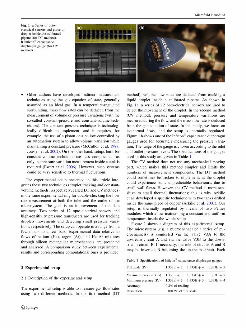
The experimental setup is able to measure gas flow rates

using two different methods. In the first method (DT

method), volume flow rates are deduced from tracking a

liquid droplet inside a calibrated pipette. As shown in

Fig. 1a, a series of 12 opto-electrical sensors are used to

detect the movement of the droplet. In the second method

(CV method), pressure and temperature variations are

measured during the flow, and the mass flow rate is deduced

from the gas equation of state. In this study, we focus on

isothermal flows, and the setup is thermally regulated.

Figure 1b shows one of the Inficon� capacitance diaphragm

gauges used for accurately measuring the pressure varia-

tion. The range of the gauge is chosen according to the inlet

and outlet pressure levels. The specifications of the gauges

used in this study are given in Table 1.

The CV method does not use any mechanical moving

part, which makes this method simpler and limits the

numbers of measurement components. The DT method

could sometimes be trickier to implement, as the droplet

could experience some unpredictable behaviours, due to

small wall flaws. However, the CV method is more sen-

sitive to small thermal fluctuations; this is why Arkilic

et al. developed a specific technique with two tanks drilled

inside the same piece of copper (Arkilic et al. 2001). Our

setup is thermally regulated by means of two Peltier

modules, which allow maintaining a constant and uniform

temperature inside the whole setup.

Figure 2 shows a diagram of this experimental setup.

The microsystem (e.g. a microchannel or a series of mi-

crochannels) is connected via the valve V3A to the

upstream circuit A and via the valve V3B to the down-

stream circuit B. If necessary, the role of circuits A and B

may be inverted, B becoming the upstream circuit. Each

Fig. 1 a Series of opto-

electrical sensors and glycerol

droplet inside the calibrated

pipette (for DT method).

b Inficon� capacitance

diaphragm gauge (for CV

method)

Table 1 Specifications of Inficon� capacitance diaphragm gauges

Full scale (Pa) 1.333E ? 3 1.333E ? 4 1.333E ? 5

Maximum pressure (Pa) 1.333E ? 3 1.333E ? 4 1.333E ? 5

Minimum pressure (Pa) 1.333E ? 2 1.333E ? 3 1.333E ? 4

Accuracy 0.2% of reading

Resolution 0.0015% of full scale


123

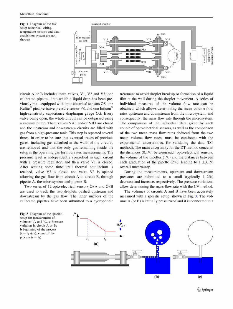
circuit A or B includes three valves, V1, V2 and V3, one

calibrated pipette—into which a liquid drop has been pre-

viously put—equipped with opto-electrical sensors OS, one

Kulite� piezoresistive pressure sensor PS, and one Inficon�

high-sensitivity capacitance diaphragm gauge CG. Every

valve being open, the whole circuit can be outgassed using

a vacuum pump. Then, valves VA3 and/or VB3 are closed

and the upstream and downstream circuits are filled with

gas from a high-pressure tank. This step is repeated several

times, in order to be sure that eventual traces of previous

gases, including gas adsorbed at the walls of the circuits,

are removed and that the only gas remaining inside the

setup is the operating gas for flow rates measurements. The

pressure level is independently controlled in each circuit

with a pressure regulator, and then valve V1 is closed.

After waiting some time until thermal equilibrium is

reached, valve V2 is closed and valve V3 is opened

allowing the gas flow from circuit A to circuit B, through

pipette A, the microsystem and pipette B.

Two series of 12 opto-electrical sensors OSA and OSB

are used to track the two droplets pushed upstream and

downstream by the gas flow. The inner surfaces of the

calibrated pipettes have been submitted to a hydrophobic

treatment to avoid droplet breakup or formation of a liquid

film at the wall during the droplet movement. A series of

individual measures of the volume flow rate can be

obtained, which allows determining the mean volume flow

rates upstream and downstream from the microsystem, and

consequently, the mass flow rate through the microsystem.

The comparison of the individual data given by each

couple of opto-electrical sensors, as well as the comparison

of the two mean mass flow rates deduced from the two

mean volume flow rates, must be consistent with the

experimental uncertainties, for validating the data (DT

method). The main uncertainty for the DT method concerns

the distances (0.1%) between each opto-electrical sensors,

the volume of the pipettes (1%) and the distances between

each graduation of the pipette (2%), leading to a ±3.1%

overall uncertainty.

During the measurements, upstream and downstream

pressures are submitted to a small (typically 1–2%)

decrease and increase, respectively. The pressure variations

allow determining the mass flow rate with the CV method.

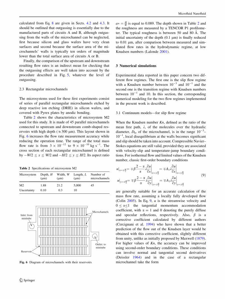
The volumes of circuits A and B have been accurately

measured with a specific setup, shown in Fig. 3. The vol-

ume A (or B) is initially pressurized and it is connected to a

V1A V2A V3A

PSA

CGA

V1B V2B V3B

PSB

CGB

Vacuumpump

High pressuregas tank

µsys

tem

Insulated chamber

Tem

pera

ture

re

gula

tion

sys

temT

emperature

regulation system

OSA

OSB

Fig. 2 Diagram of the test

setup (electrical wiring,

temperature sensors and data

acquisition system are not

shown)

Fig. 3 Diagram of the specific

setup for measurement of

volumes VA and VB. a Pressure

variation in circuit A or B;

b beginning of the process

(t = t1 ? e); c end of the

process (t = t2)


123

balloon using a tube with a small diameter. This balloon

has been previously filled with water and turned upside

down on a basin of water. The connection of the small tube

is at the level of the water surface, such that the pressure

inside the tube is equal to the atmospheric pressure Patm.

The valve is opened at t = t1 to allow the air flow from the

circuit A (or B) towards the balloon (Fig. 3b). The balloon

is slowly filled with air and the valve is closed at t = t2when all the water inside the balloon has been replaced

with air (Fig. 3c). During this process, the pressure PA,B

inside the volume A (or B) is monitored with a piezore-

sistive sensor PS (see typical pressure signal in Fig. 3a).

The volume VA,B of the circuit A (or B) can then be

deduced from the mass conservation, assuming that air

behaves as an ideal gas, by the equation

VA;B ¼PatmVballoon

DPA;Bð1Þ

where DPA,B is the pressure variation inside the volume A

(or B) between times t1 and t2. The volume Vballoon includes

the volume of the balloon and the volume of the tube

between the valve and the balloon. This volume has been

measured by weighting the balloon and the tube before and

after filling them with water. The uncertainty on the

volume of circuit A (or B) is then estimated as:

DVA;B

VA;B¼

D DPA;B

� �

DPA;Bþ DPatm

Patm

þ DVballoon

Vballoon

¼ � 0:5þ 0:5þ 0:3ð Þ% ¼ �1:3%: ð2ÞAccording to the range of the measured flow rate and the

duration of the measure, these volumes can be adjusted

changing some internal parts of circuits A and B between

valves V1 and V2.

The temperature variation is measured during the

operations with four PT100 temperature sensors (with a

0.15 K accuracy), and the deviation during each experi-

ment is less than 0.1 K. The temperature inside the insu-

lated chamber is homogeneous with deviations less than

0.6 K.

Most of the setup is made of stainless steel, aluminium

or glass, and the connections are insured by ISO-KF and

Swagelok’s Ultra-Torr� components to avoid any leakage

during low-pressure operation. Air tightness has been

checked by means of He detection, with a portable high

precision leak detector.

2.2 Flow rate calculation

2.2.1 CV method

With the constant volume method, the mass flow rate is

calculated from the ideal-gas equation of state

dM

dt¼ d

dt

PV

RT

� �ð3Þ

applied to circuit A or B, where M, V, P, R, T and t are,

respectively, the mass of the gas in the circuit, the constant

volume of the circuit, the pressure, the specific gas

constant, the temperature and the time. The mass flow

rate through the microsystem is then given by (Arkilic et al.

2001; Ewart et al. 2006)

_M ¼ V

RT

dP

dt1� dT=T

dP=P

� �: ð4Þ

As mentioned earlier, this method requires a high-thermal

stability, ensured by two temperature-regulation systems

(see Fig. 2). The standard deviation of the temperature is in

all cases around 0.1 K. The relative temperature variation

dT/T is then of the order of 4 9 10-4 (see Fig. 4), to be

compared with the relative pressure variation dP/P &2 9 10-2. As a consequence, Eq. 4 is simplified as

_M ¼ V

RTac ð5Þ

where a = dP/dt is calculated from a least-square linear fit

of the measured pressure

P tð Þ ¼ at þ b ð6Þ

and c = 1-(dT/T)/(dP/P) = 1 ± 2%. More than 1,000

pressure data are used for determining coefficients a and b.

The standard deviation of coefficient a is calculated

following the method proposed in (Ewart et al. 2006) and

is found to be less than 0.5%. Therefore, the overall

uncertainty of the mass flow rate measurement is calculated

from

D _M

_M¼ DV

Vþ DT

Tþ Da

aþ Dc

c; ð7Þ

and is less than ±(1.3 ? 0.2 ? 0.5 ? 2)% = ±4%.

2.2.2 Operating procedure and data processing

for CV method

Outgassing from the setup when operating at low pressure

could generally not be neglected, and consequently must be

measured. Outgassing is first quantified in the downstream

circuit B, including all connections up to the microsystem

outlet. In order to avoid flow through the microsystem during

this operation, both upstream and downstream circuits are

pressurized to the downstream operating pressure before

closing valve V3A. After registering with gauge CGB, the

pressure rise in circuit B during a while (see 1st step in

Fig. 5), pressure in circuit A is increased to the desired

upstream value and the flow rate through the microsystem

can be measured opening valve V3A. Following the flow rate


123

measurement (see 2nd step in Fig. 5), outgassing is quanti-

fied in circuit A, including all connections up to the micro-

system inlet. For that purpose, pressure in circuit B is

increased to the same level as in circuit A, to avoid flow

through the microsystem due to a pressure gradient; then

valve V3B is closed and the pressure rise in circuit A is

monitored for some time by gauge CGA (see 3rd step in

Fig. 5). The operating time of flow measurement ranges

between several minutes and 2 h, depending on pressure

conditions. However, the outgassing evaluation process

could take around 3 h in order to detect a small pressure

variation. During all this process, the test rig is kept at

constant temperature as illustrated by Fig. 4 thus showing

that the temperature inside the thermal box is not sensitive to

possible variations of the room temperature. Figure 5 rep-

resents schematically the operating procedure and data

processing for the CV method. Outgassing rates are calcu-

lated with Eq. 5 and used to correct the flow rate data.

Outgassing is negligible for moderate Knudsen numbers

(mean values less than 10-1), but the corresponding flow

rates can reach 60% of the real flow rates through the

microchannels for the highest Knudsen numbers. The

uncertainties shown in Eq. 7 are also taken into account for

the calculation of the outgassed flow rate, and the total

uncertainty represented by vertical bars in the following

figures takes into account all uncertainties introduced in the

three steps of the operating procedure shown in Fig. 5. As a

consequence, for the highest values of the outlet pressure

(50 kPa), the total uncertainty is ±4% as outgassing is

negligible, and for lower outlet pressures for which outgas-

sing is no longer negligible, the total uncertainty is given by

D _M

_M¼ �0:04 1þ 2

_Moutgass:

_M

� �ð8Þ

where _Moutgass: is the mass flow rate inside circuit A or B

only due to outgassing (see Fig. 5). The uncertainties

297

297.5

298

298.5

299

299.5

0 60 120 180 240 300 360

t (min)

T (

K)

Fig. 4 Typical temperature

evolution inside the insulated

chamber

OPERATION

Outgassingevaluationin circuit B

Outgassingevaluationin circuit A

Flowratemeasurement

1st Step 2nd Step 3rd Step

A

A

VRT

DATA PROCESSING

-

+-

A

A

VRT

B

B

VRT

B

B

VRT

AP t∆ ∆

AP t∆ ∆

BP t∆ ∆

BP t∆ ∆

.A outgassM M=

MM

MM

M M

-

Comparison

.

A

B

B outgass=

Fig. 5 Schematic

representation of operating

procedure and data processing

(case for which A is the

upstream circuit)


123

calculated from Eq. 8 are given in Sects. 4.2 and 4.3. It

should be outlined that outgassing is essentially due to the

manufactured parts of circuits A and B, although outgas-

sing from the walls of the microchannel can be neglected,

first because silicon and glass wafers have very clean

surfaces and second because the surface area of the mi-

crochannels’ walls is typically ten orders of magnitude

lower than the total surface area of circuits A or B.

Finally, the comparison of the upstream and downstream

resulting flow rates is an indirect mean for checking that

the outgassing effects are well taken into account by the

procedure described in Fig. 5, whatever the level of

outgassing.

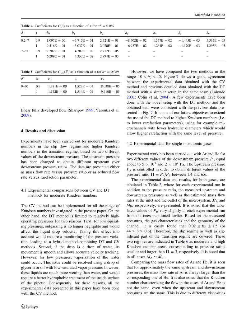
2.3 Rectangular microchannels

The microsystems used for these first experiments consist

of series of parallel rectangular microchannels etched by

deep reactive ion etching (DRIE) in silicon wafers, and

covered with Pyrex plates by anodic bonding.

Table 2 shows the characteristics of microsystem M2

used for this study. It is made of 45 parallel microchannels

connected to upstream and downstream comb-shaped res-

ervoirs with high depth (&300 lm). This layout shown in

Fig. 6 increases the flow rate measurement accuracy while

reducing the operation time. The range of the total mass

flow rate is from 3 9 10-12 to 9 9 10-10 kg s-1. The

cross section of each rectangular microchannel is defined

by -W/2 B x B W/2 and -H/2 B y B H/2. Its aspect ratio

a� ¼ HW is equal to 0.089. The depth shown in Table 2 and

the roughness are measured by a TENCOR P1 profilome-

ter. The typical roughness is between 50 and 80 A. The

initial uncertainty of the depth (0.1 lm) is finally reduced

to 0.01 lm, after comparison between measured and sim-

ulated flow rates in the hydrodynamic regime, at low

Knudsen numbers (Lalonde 2001).

3 Numerical simulations

Experimental data reported in this paper concern two dif-

ferent flow regimes. The first one is the slip flow regime

with a Knudsen number between 10-3 and 10-1 and the

second one is the transition regime with Knudsen numbers

between 10-1 and 10. In this section, the corresponding

numerical modeling for the two flow regimes implemented

in the present work is described.

3.1 Continuum models—for slip flow regime

When the Knudsen number Kn, defined as the ratio of the

mean free path, k, of the molecules over the hydraulic

diameter, Dh, of the microchannel, is in the range 10-3–

10-1, local disequilibrium at the walls becomes significant

and slip should be taken into account. Compressible Navier–

Stokes equations are still valid, provided they are associated

with velocity-slip and temperature-jump boundary condi-

tions. For isothermal flow and limited values of the Knudsen

number, classic first-order boundary conditions

ujx¼�W2¼ �b

2� aa

kou

ox

��x¼�W

2

¼ �A1kou

ox

��x¼�W

2

ujy¼�H2¼ �b

2� aa

kou

oy

��y¼�H

2

¼ �A1kou

oy

��y¼�H

2

ð9Þ

are generally suitable for an accurate calculation of the

mass flow rate, assuming a locally fully developed flow

(Colin 2005). In Eq. 9, u is the streamwise velocity and

0 B aB1 the tangential momentum accommodation

coefficient, with a = 1 and 0 denoting the purely diffuse

and specular reflections, respectively. Also, b is a

corrective coefficient calculated by different authors

(Cercignani et al. 1994) who have shown that a better

prediction of the flow out of the Knudsen layer would be

obtained with this corrective coefficient, slightly different

from unity, unlike as initially proposed by Maxwell (1879).

For higher values of Kn, the accuracy can be improved

using second-order boundary conditions. These conditions

can involve normal and tangential second derivatives

(Deissler 1964) and in the case of a rectangular

microchannel take the form

Table 2 Specifications of microsystem M2

Microsystem Depth, H(lm)

Width, W(lm)

Length, L(lm)

Number of

microchannels

M2 1.88 21.2 5,000 45

Uncertainty 0.10 0.3 10

Inlet: from minitube

Outlet: to minitube

Reservoir

Microchannels

Fig. 6 Diagram of microchannels with their reservoirs


123

ujx¼�W2¼�A1k

ou

ox

��x¼�W

2

þA2k2 o2u

ox2þB2

o2u

oy2

� ��x¼�W

2

ujy¼�H2¼�A1k

ou

oy

��y¼�H

2

þA2k2 o2u

oy2þB2

o2u

ox2

� ��y¼�H

2

:

ð10Þ

In the present paper, experimental data are compared

with semi-analytical models of flows in rectangular

microchannels based on boundary conditions (9) or (10).

It is noted that the first-order coefficient in Eq. 10 is

A1 = b(2 - a)/a. Values of coefficients b, A2 and B2 are

shown in Table 3. For first-order boundary conditions, the

coefficient A2 is zero. Maxwell (1879) proposed b = 1 and

Cercignani and Daneri (1963) further obtained an

improved value b = 1.1466 from the BGK equation.

Deissler developed a second-order boundary condition

valid for 3-D flows, with the coefficients b = 1, A2 = -9/

8 and B2 = 1/2. Recently, Hadjiconstantinou (2003)

suggested to keep the value b = 1.1466 from Cercignani

and to modify A2 as A2 = -0.647. In this paper, we

propose a modified second-order boundary conditions (see

Table 3), taking into account the coefficients from

Hadjiconstantinou, associated with the value B2 = 1/2

proposed by Deissler. In all cases, the mean free path is

calculated based on the hard sphere collision model

(Chapman and Cowling 1952; Kandlikar et al. 2006).

Aubert and Colin (2001) proposed a semi-analytical

model for calculating the mass flow rate through a rect-

angular microchannel using Deissler boundary conditions.

After integration along the microchannel, the mass flow

rate initially calculated as a function of the local pressure

gradient can be obtained as a function of the total inlet over

outlet pressure ratio P ¼ PA

PB:

_M ¼ � 4h4

a�lL

P2B

RT

�a1 P2 � 1� �

2þ a2KnB P� 1ð Þ þ a3Kn2

B ln P

!

:

ð11Þ

In Eq. 11, l is the dynamic viscosity of the gas,

subscript B refers to the outlet of the microchannel, the

length of which is L, the coefficients (a1, a2, a3) depend

on the aspect ratio a* and (a2, a3) depend on the

accommodation coefficient a. For a* = 0.089 and a = 0.9,

a1 Dð Þ ¼ 0:3147; a2 D;a¼0:9ð Þ ¼ 2:3954; a3 D;a¼0:9ð Þ ¼ 4:1352

ð12Þ

are obtained from the model developed in (Aubert and

Colin 2001). For a* = 0.089 and a = 1, their values are:

a1 Dð Þ ¼ 0:3147; a2 D;a¼1ð Þ ¼ 1:9819; a3 D;a¼1ð Þ ¼ 4:1344:

ð13Þ

In Eqs. 12 and 13, subscript D refers to Deissler

boundary conditions. The same semi-analytical model has

been applied for the modified boundary conditions

proposed earlier. For these boundary conditions, we

obtain for a* = 0.089 and a = 1

a1 mð Þ ¼ 0:3134; a2 m;a¼1ð Þ ¼ 2:2139; a3 m;a¼1ð Þ ¼ 2:4212:

ð14Þ

In the present paper, experimental flow rates are compared

with the values given by Eq. 11 and the coefficients

associated to Deissler boundary conditions [Eqs. 12 or 13]

or to the modified boundary conditions [Eq. 14].

3.2 Kinetic models—for whole Knudsen range

Solutions based on kinetic theory of gases are valid in the

whole range of the Knudsen number from the free

molecular, through the transition up to the slip and

hydrodynamic regimes. The basic unknown is the distri-

bution function, which obeys the Boltzmann equation or

reliable and properly chosen kinetic model equations. Over

the years, it has been shown that fully developed isother-

mal pressure driven flows, as the ones investigated in the

present work, can be simulated efficiently by the linearized

BGK equation, which in dimensionless form is written as

(Sharipov 1999)

Table 3 Values of coefficients b, A2 and B2 for boundary conditions (9) or (10)

Author, year b A2 B2 Remarks

Maxwell, 1879 (Maxwell 1879) 1 0 – First-order model

Cercignani, 1963 (Cercignani and

Daneri 1963)

1.1466 0 – From kinetic theory—BGK equation

Deissler, 1964 (Deissler 1964) 1 -9/8 1/2 Second-order model

Hadjiconstantinou, 2003

(Hadjiconstantinou 2003)

1.1466 -0.647 – From kinetic theory—BGK equation

Modified second-order boundary

conditions (present paper)

1.1466 -0.647 1/2 Deissler boundary conditions modified

with Hadjiconstantinou’s coefficients


123

cxoUoxþ cy

oUoyþ dU ¼ du� 1

2: ð15Þ

Here, U = U (x, y, cx, cy) is the reduced unknown

distribution, while (cx, cy) denote the components of the

molecular velocity vectors in the x- and y-directions. Also,

u x; yð Þ ¼ 1

p

Z1

�1

Z1

�1

U exp �c2x � c2

y

h idcxdcy ð16Þ

is the streamwise macroscopic (bulk) velocity. The

rarefaction parameter d characterizes the flow and it is

given by

d ¼ffiffiffipp

2

1

Kn¼

ffiffiffipp

2

Dh

k¼ DhP

lt; ð17Þ

where P = P(z) is the pressure along the microchannel, l is

the gas viscosity at temperature T and t ¼ffiffiffiffiffiffiffiffiffi2RTp

is the most

probable molecular velocity. It is seen that d is proportional

to the inverse Knudsen number, i.e. d = 0 and d ? ?correspond to the free molecular and hydrodynamic limits,

respectively. The gas–wall interaction is modeled by the

Maxwell diffuse–specular reflection condition. At the

boundaries we have (Naris and Valougeorgis 2008)

Uþ ¼ 1� að ÞU� ð18Þ

where U? and U- are the distributions representing parti-

cles departing and arriving at the wall, respectively, while

the tangential momentum accommodation coefficient adenotes the portion of the particles reflecting diffusively

from the wall.

The kinetic problem described by Eqs. 15 and 16 and

the associated boundary condition 18 is solved numerically

in an iterative manner. The numerical scheme has been

presented, in detail, in previous works (Sharipov 1999;

Naris and Valougeorgis 2008) and, therefore, only the key

elements are presented here for completeness purposes.

The two components of the molecular velocity vector are

written in terms of polar coordinates as cx = f cos h and

cy = f sin h, where 0 B f B ? is its magnitude and

0 B hB2p its polar angle. Then, the discretization in the

molecular velocity space is performed by choosing a suit-

able set of discrete velocities (fm, hn), defined by

0 B fm \? and 0 B hn B 2p, with m = 1,2,…, M and

n = 1,2,…, N. Introducing this discretization into Eqs. 15

and 16, yields a system of partial differential equations

fm cos hn

oU kþ1=2ð Þm;n

oxþ fm sin hn

oU kþ1=2ð Þm;n

oyþ dU kþ1=2ð Þ

m;n

¼ du kð Þ � 1

2ð19Þ

coupled with the double summations

u kþ1ð Þ ¼X

n

X

m

wmwnUkþ1=2ð Þ

m;n ; ð20Þ

where wm and wn are the weighting factors corresponding

to the integration over fm and hn, respectively.

Equations 19 and 20 are solved in an iterative manner,

with the superscript k denoting the iteration index. First, the

macroscopic velocity u(k) is assumed at the right-hand side

of Eq. 19, which is solved for the distribution function

Um,n(k?1/2). Then, the distribution function is introduced into

Eq. 20 to compute the updated values of the macroscopic

velocity u(k?1). This iteration map is terminated when the

convergence criterion is fulfilled. In several occasions, it is

necessary to speed up the convergence of the iteration

scheme by introducing a synthetic diffusion acceleration

scheme introduced in (Valougeorgis and Naris 2003). In

each iteration, the system of partial differential equa-

tions 19 is solved by implementing a second-order central

finite difference scheme in the physical space. It is

important to note that the system is solved in an explicit

manner using a marching procedure and no matrix inver-

sion is required. The implemented numerical algorithm,

supplemented by a reasonable dense grid and an adequate

large set of discrete velocities, deduces grid-independent

results up to several significant figures with modest com-

putational effort.

Once the above-described dimensionless kinetic prob-

lem is solved, several dimensional quantities of practical

interest may be recovered in a straightforward manner. For

the purposes of the present work, we focus on the mass

flow rate, which is calculated from (Sharipov and Seleznev

1998; Varoutis et al. 2009) by

_M ¼ G~ADh

tdP

dz: ð21Þ

Here, Dh and ~A are the hydraulic diameter and the cross

section area of the microchannel. The quantity G is

traditionally known as reduced (or dimensionless) flow rate

and it is defined by (Sharipov and Seleznev 1998)

G ¼ 2

A

ZZ

A

u dA ð22Þ

with A ¼ ~A=D2h denoting the dimensionless cross-section

area. The kinetic solution, which finally results in the cal-

culation of G, depends only on d, A, and a.

In the present work, the measured mass flow rates are

compared with the computed ones. For this purpose, two

approaches are compared. Both of them deduce practically

identical results. In the first approach, the mass flow rate is

calculated by

_M ¼ G�~ADh

tPA � PB

L: ð23Þ


123

The quantity G* is computed from the kinetic solver using

the specific dimensionless cross section A and an average

rarefaction parameter d0 = (dA ? dB)/2, where dA and dB

correspond to pressures PA and PB, respectively, while the

accommodation coefficient, a, may vary depending on the

roughness of the channel wall. In the same way, the average

Knudsen number is defined as Kn0 ¼ffiffiffipp

=2d0:

In an alternative approach, the variation of the pressure

gradient along the microchannel is taken into account. For

that purpose, the value of the reduced flow rate G(d) is

calculated as a function of d which varies along the mi-

crochannel. The function G(d) is fitted with a polynomial

approximation as

G dð Þ ¼ b0 þ b1dþ b2d2 þ b3d

3 þ b4d4 þ b5d

5 þ b6d6:

ð24Þ

Then, Eq. 21 could be written as

_M ¼ Dh HBð Þt

dP

dzb0 þ b1dþ b2d

2 þ b3d3

�

þb4d4 þ b5d

5 þ b6d6�: ð25Þ

For an isothermal flow, the ratio of P/d is constant along

the microchannel:

P

d¼ PB

dB

: ð26Þ

Then Eq. 25 becomes

_M ¼ Dh HBð Þt

dP

dz

� b0 þ b1dB

P

PB

þ b2d2B

P

PB

� �2

þb3d3B

P

PB

� �3

þb4d4B

P

PB

� �4

þb5d5B

P

PB

� �5

þb6d6B

P

PB

� �6!

: ð27Þ

After integration along the microchannel,

_M ¼ Dh HBð Þt

PB

Lb0 P� 1ð Þ þ b1

dB

2P2 � 1� ��

þb2

d2B

3P3 � 1� �

þ b3

d3B

4P4 � 1� �

þ b4

d4B

5P5 � 1� �

þb5

d5B

6P6 � 1� �

þ b6

d6B

7P7 � 1� ��

: ð28Þ

Due to the shape of G(d), the polynomial approximation

has been done separately for two ranges of the rarefaction

number. Corresponding values of coefficients bi are given

in Table 4. Simulated data obtained from Eqs. 23 and 28

have been compared. In most cases, the deviation between

the two models has been found negligible: the difference

between the two theoretical _MðPÞ curves was less than the

width of the line. All the following figures represent kinetic

results obtained from Eq. 28.

The kinetic analysis and solution methodology descri-

bed above have been extended to the case of binary gas

mixtures through rectangular channels based on the Mc-

Cormack model (Naris et al. 2005). It is interesting to

note that for gas mixtures, the imposed pressure gradient

produces two types of flow. The first one, denoted by

GPP, is the well-known Poiseuille flow; it is a direct effect

and it is the one, which has been extensively studied in

the case of single gases. The second one, denoted by GCP,

is known as barodiffusion and it is a cross effect, which

disappears as the flow is approaching the hydrodynamic

limit. Following (Naris et al. 2005) both dimensionless

flow rates may be computed. Then, dimensionalizing the

results it is deduced that the combined mass flow rate is

given by

_M ¼ G�PP þ G�BD½ �PA � PB

L

H HWð Þt

¼ G�Cal

PA � PB

L

H HWð Þt

; ð29Þ

where

G�BD ¼ �m2 � m1ð Þ

m1� C0ð ÞG�CP ð30Þ

C0 is the molar concentration of the mixture, m1 and m2 are

the molecular masses of the two species and

m ¼ m1C0 þ 1� C0ð Þm2 ð31Þ

is the molecular mass of the mixture. As in the case of

simple gases, in order to avoid an estimation of G*PP and

G*CP based on a mean value of d0 ¼ d HDh; the mass flow

rate can also be obtained by integration of

_M ¼ GCal d0ð Þ dP

dz

H HWð Þt

; ð32Þ

which leads to

_M ¼ H HBð Þt

PB

L

� c0 P� 1ð Þ þ c1

d0B2

P2 � 1� �

þ c2

d02B

3P3 � 1� �

!

;

ð33Þ

after a polynomial fit of GCal(d0) = GPP(d0) ? GBD(d0).Values of coefficients ci are given in Table 5, and Sect. 4.3

provides a comparison between data obtained from Eqs. 29

and 33.

Closing this section, it is noted that the implementation

of the linearized BGK and McCormack models for solving

rarefied flows through microchannels is valid, not only in

small but even at arbitrarily large pressure drops, provided

that the ratio of the hydraulic diameter over the length of

the channel is much less than one. This is the same

assumption which allows the modeling of the flow as a


123

linear fully developed flow (Sharipov 1999; Varoutis et al.

2009).

4 Results and discussion

Experiments have been carried out for moderate Knudsen

numbers in the slip flow regime and higher Knudsen

numbers in the transition regime, based on two different

values of the downstream pressure. The upstream pressure

has been changed to obtain different upstream over

downstream pressure ratios. The data are presented either

as mass flow rate versus pressure ratio or as reduced flow

rate versus rarefaction parameter.

4.1 Experimental comparisons between CV and DT

methods for moderate Knudsen numbers

The CV method can be implemented for all the range of

Knudsen numbers investigated in the present paper. On the

other hand, the DT method is limited to relatively high-

operating pressures for two reasons. First, for low-operat-

ing pressures, outgassing is no longer negligible and would

affect the liquid drop velocity. Taking this effect into

account would require a monitoring of the pressure varia-

tion, leading to a hybrid method combining DT and CV

methods. Second, if the drop is a drop of water, its

movement is smooth and allows accurate velocity tracking.

However, for low pressures, vaporization of the water

could occur. This issue could be resolved using a drop of

glycerin or oil with low-saturated vapor pressure; however,

these liquids are much more wetting than water, and would

require a better hydrophobic treatment of the inside surface

of the pipette. Consequently, for these reasons, all the

experimental data presented in this paper have been done

with the CV method.

However, we have compared the two methods in the

range 10 \ d0 \ 45. Figure 7 shows a good agreement

between the experimental data obtained with the CV

method and previous detailed data obtained with the DT

method with a simpler setup in the same team (Lalonde

2001; Colin et al. 2004). A few experiments have been

done with the novel setup with the DT method, and the

obtained data were consistent with the previous data pre-

sented in Fig. 7. It is one of our future objectives to extend

the use of the DT method to higher Knudsen numbers (i.e.

to lower rarefaction parameters), using for example mi-

crochannels with lower hydraulic diameters which would

allow higher rarefaction with the same level of pressure.

4.2 Experimental data for single monatomic gases

Experimental work has been carried out with Ar and He for

two different values of the downstream pressure PB equal

about to 5 9 104 and 2 9 103 Pa. The upstream pressure

PA is controlled in order to obtain different values of the

pressure ratio P = PA/PB between 1.4 and 6.6.

The experimental data and results, for both gases, are

tabulated in Table 2, where for each experimental run in

addition to the pressure ratio, the measured upstream and

downstream pressures as well as the estimated mass flow

rates at the inlet and the outlet of the microsystem, _MA and_MB, respectively, are presented. It is noted that the tabu-

lated values of PB vary slightly at each experimental run

from the ones mentioned earlier. Based on the measured

pressures, the gas characteristics and the geometry of the

channel, it is easily found that 0.02 B Kn B 1.5 (or

44 C d C 0.6). Therefore, the slip regime as well as sig-

nificant part of the transition regime are covered. These

two regimes are indicated in Table 6 as moderate and high

Knudsen number areas, corresponding to pressure ratios

smaller and larger than P = 3, respectively. It is noted that

in all cases _MA ’ _MB:

Comparing the mass flow rates of Ar and He, it is seen

that for approximately the same upstream and downstream

pressures, the mass flow rate of Ar is always larger than the

corresponding one of He. It is also noted that the Knudsen

number characterizing the flow in the cases of Ar and He is

not the same, even when the upstream and downstream

pressures are the same. This is due to different viscosities

Table 5 Coefficients for GCal(d0) as a function of a for a* = 0.089

d0 a c0 c1 c2

9–30 0.9 1.371E ? 00 1.523E - 01 8.038E - 05

1 1.172E ? 00 1.514E - 01 9.410E - 05

Table 4 Coefficients for G(d) as a function of a for a* = 0.089

d a b0 b1 b2 b3 b4 b5 b6

0.2–7 0.9 1.097E ? 00 -3.715E - 01 2.521E - 01 -8.502E - 02 1.557E - 02 -1.445E - 03 5.312E - 05

1 9.516E - 01 -3.037E - 01 2.070E - 01 -6.927E - 02 1.264E - 02 -1.170E - 03 4.295E - 05

7–65 0.9 7.207E - 01 4.387E - 02 2.717E - 05 – – – –

1 6.209E - 01 4.357E - 02 2.994E - 05 – – – –


123

0.5

1

1.5

2

2.5

3

8.00E+00 1.80E+01 2.80E+01 3.80E+01 4.80E+01

δ 0

G*

Kinetic model: Linearized BGKα = 1

Kinetic model: Linearized BGKα = 0.9

Continuum model:Deissler 2nd-order BCα = 1

Continuum model:Deissler 2nd-order BCα = 0.9

Continuum model:Maxwell 1st-order BCα = 1

Continuum model:Modified 2nd-order BCα = 1

Continuum model:Cercignani 1st-order BCα = 1

Fig. 7 Reduced flow rate

versus rarefaction factor.

Experimental data obtained with

the CV method: inlet (filledsquare) and outlet (opensquare) data for helium and

inlet (filled diamond) and outlet

(open diamond) data for argon,

detailed in Figs. 11 and 12.

Experimental data obtained with

the DT method: inlet (filledtriangle) and outlet (opentriangle) data for helium, from

(Lalonde 2001). Comparison

with kinetic and continuum

models

Table 6 Experimental data, for Argon and Helium at constant temperature T = 298.5 K

Kn0 P PA PB_MA

_MB Uncertainty (%)

Pa kg/s A B

Argon

Moderate Knudsen number 2.1E - 02 2.99 149,687 50,074 1.95E - 11 1.97E - 11 4.0 4.0

2.4E - 02 2.50 125,056 49,927 1.37E - 11 1.34E - 11 4.0 4.0

2.8E - 02 1.98 99,288 50,169 7.80E - 12 7.88E - 12 4.0 4.0

3.0E - 02 1.79 89,862 49,828 6.09E - 12 6.19E - 12 4.0 4.0

3.2E - 02 1.60 80,124 50,158 4.28E - 12 4.39E - 12 4.0 4.0

3.4E - 02 1.38 69,764 50,399 2.5E - 12 2.7E - 12 4.0 4.0

High Knudsen number 2.6E - 01 6.61 13,569 2,052 7.47E - 13 7.18E - 13 6.0 6.6

3.0E - 01 5.96 11,857 1,990 6.06E - 13 6.05E - 13 6.8 7.5

3.5E - 01 4.79 9,754 2,036 4.84E - 13 4.77E - 13 7.3 7.8

4.2E - 01 4.02 7,879 1,962 3.59E - 13 3.49E - 13 8.6 8.6

5.0E - 01 3.10 6,198 2,002 2.66E - 13 2.55E - 13 9.7 9.6

Helium

Moderate Knudsen number 5.7E - 02 2.90 148,460 51,190 3.26E - 12 3.09E - 12 4.0 4.0

6.5E - 02 2.42 123,610 50,990 2.26E - 12 2.13E - 12 4.0 4.0

7.6E - 02 1.95 98,760 50,540 1.38E - 12 1.31E - 12 4.0 4.0

8.1E - 02 1.72 88,440 51,300 1.06E - 12 9.68E - 13 4.0 4.0

8.8E - 02 1.58 79,150 50,210 8.00E - 13 7.37E - 13 4.0 4.0

9.5E - 02 1.44 70,373 48,890 5.79E - 13 5.39E - 13 4.0 4.0

High Knudsen number 7.3E - 01 6.81 13,489 1,982 2.16E - 13 2.20E - 13 4.5 4.9

8.4E - 01 5.83 11,576 1,985 1.87E - 13 1.84E - 13 4.8 5.0

9.4E - 01 4.97 10,015 2,015 1.53E - 13 1.52E - 13 5.1 5.3

1.1E ? 00 3.92 7,870 2,008 1.14E - 13 1.09E - 13 5.6 6.0

1.4E ? 00 3.12 6,020 1,928 7.78E - 14 7.82E - 14 6.6 6.4


123

and molecular velocities. Actually, for the same pressure

set up, the Knudsen number for the light gas is larger.

We continue with a detailed comparative study between

experiments and calculations presented in Figs. 8, 9, 10, 11,

12. First, an overall view of the experimental and the

associated computed results is shown in Fig. 8, where the

reduced flow rate G is plotted in terms of the rarefaction

parameter d0. Experimental data obtained with Ar and He

are represented with diamond-shaped and square symbols,

respectively. Experimental uncertainties on G, deduced

from the uncertainties of the mass flow rate _M (see Eq. 7),

are represented by vertical bars. Also, continuum and kinetic

model computed results are provided for a = 1 and 0.9.

It is observed that the experimental data are in very good

agreement with the kinetic model based on the linearized

BGK equation, with a = 1, in the whole range of d for both

Ar and He. It is interesting to note that based on the

experimental work, we may deduce that for both gases the

interaction with the wall is purely diffusive. Regarding

the continuum models, it is seen that all models perform

quite well for d0 C 20, while as d0 is further decreased

they gradually deviate from the measured flow rate. In

particular, the first-order model underestimates, while the

second-order models overestimate the values of G. It may

be argued, as it is seen from the modified boundary con-

ditions, that for this specific problem, second-order models

remain reliable even for values of d0 a little bit less than 10.

Ewart et al. studied the flow of monatomic gases

through rectangular microchannels with a low-aspect ratio

a* = 2% (Ewart 2007; Ewart et al. 2007). With such an

aspect ratio, the flow is close to a 2-D flow between parallel

plates. The authors found a good agreement between their

experimental data and a kinetic BGK model, down to an

average rarefaction parameter d0 & 0.2. A quantitative

comparison of their data with the present data is not pos-

sible, as the rectangular microchannel considered here has

a high-aspect ratio a* = 9% which leads to non-negligible

3-D effects. However, Fig. 8 extends the main conclusions

from Ewart et al., showing that a kinetic BGK model is

accurate for gas flows in rectangular microchannels.

The results of Table 6 and Fig. 8 are examined more

thoroughly in Figs. 9, 10, 11, 12, where the mass flow rates_M are plotted in terms of the pressure ratio P. In particular,

the results for the high Knudsen number (d0 \ 5), corre-

sponding to a pressure ratio from 3 to 7, are plotted in

Fig. 9 for Ar and in Fig. 10 for He. Similarly, the results

for the moderate Knudsen number (d0 [ 5), corresponding

to a pressure ratio from 1.4 to 3, are plotted in Fig. 11 for

Ar and in Fig. 12 for He. The range of the average

Knudsen number is indicated in the legend of each figure.

As the downstream pressure PB can slightly differ at

each experimental run (within ±2% around the values

2 9 103 Pa, in Figs. 9 and 10, or around 5 9 104 Pa, in

Figs. 11 and 12), and as the mass flow rate depends both on

the pressure ratio and on the downstream pressure, all

theoretical data have been calculated for the exact values

of PB provided in Table 6. This is the reason why some

theoretical curves can experience small irregularities.

The very good agreement between experimental and

kinetic results, with a = 1, is clearly demonstrated through

all Figs. 9, 10, 11, 12. Also, the effect of the tangential

momentum accommodation coefficient on the mass flow

rates may be observed by comparing the kinetic results

for a = 1 with the corresponding ones for a = 0.9. As

0

0.5

1

1.5

2

2.5

3

1.00E-01 1.00E+00 1.00E+01 1.00E+02

δ 0

G*





Continuum model:Maxwell 1st-order BCα = 1


Continuum model:Cercignani 1st-order BCα = 1

Figure 10

Figure 11

Figure 9

Figure 12

Fig. 8 Reduced flow rate

versus rarefaction factor.

Comparison between inlet

(filled square) and outlet (opensquare) data for helium and

inlet (filled diamond) and outlet

(open diamond) data for argon

with kinetic and continuum

models. Data from Table 6.

T = 298.5 K


123

expected, as the rarefaction is increased, the dependency of_M on a is also increased.

In Fig. 9, the limits of the continuum model with second-

order boundary conditions from Deissler are clearly pointed

out. It is seen that the discrepancy between second-order slip

theory and measurements (or kinetic theory) is significant.

The modified second-order boundary conditions provide

improved results, which are closer to the kinetic results, but

again the correct values of the flow rates are overestimated.

Similar observations can be made in the case of He, in

Fig. 10. Here, as mentioned earlier, the corresponding

Knudsen numbers are higher compared to the ones in the

experiment with Ar, and, therefore, the discrepancy

between the continuum model and measured (or kinetic

theory) flow rates becomes more significant. For this rea-

son, we have decided not to show the continuum results in

this figure since they are out of the scale used in the figure.

On the other hand, for moderate Knudsen numbers as

the ones in Figs. 11 and 12 continuum models perform

much better. In particular, the modified second-order slip

model is in very good agreement with the experimental

results, assuming a = 1, as it is also found with the BGK

kinetic model. Although the accommodation coefficient

can be determined with a precision of a few percents only,

0.0E+00

2.0E-13

4.0E-13

6.0E-13

8.0E-13

1.0E-12

1.2E-12

3.00 3.50 4.00 4.50 5.00 5.50 6.00 6.50 7.00

Π

M(k

g/s)

.






Fig. 9 Mass flow rate versus

pressure ratio for argon.


(filled diamond) and outlet

(open diamond) data with

kinetic and continuum models.

Data from Table 6.

T = 298.5 K,

PB & 2 9 103 Pa,

0.25 \ Kn0 \ 0.5,

1.7 \ d0 \ 3.4

0.0E+00

5.0E-14

1.0E-13

1.5E-13

2.0E-13

2.5E-13

3.0E-13

3.00 3.50 4.00 4.50 5.00 5.50 6.00 6.50 7.00

Π

M(k

g/s)

.Kinetic model: Linearized BGKα = 1



pressure ratio for helium.


(filled square) and outlet (opensquare) data with kinetic

models. Data from Table 6.

T = 298.5 K,

PB & 2 9 103 Pa,

0.7 \ Kn0 \ 1.5,

0.6 \ d0 \ 1.2


123

due to experimental uncertainties, it could be concluded

that in average, the accommodation of the gas molecules

on the microchannel walls is essentially diffuse.

4.3 Data on binary mixture

A first set of experimental data for a binary mixture of

monatomic gases is now presented in Fig. 13. The mixture

is composed of 30% He and 70% Ar. In these experiments,

the Knudsen number is less than 0.04 and therefore, the

flow is in the slip regime. Tabulated results are presented in

Table 7, where experimental and kinetic results may be

compared. The agreement is very good. In addition, the

portion of the flow which is due to the classical Poiseuille

flow and due to barodiffusion indicated by G*PP and G*BD,

respectively, are specified in the last two columns of the

table. It is seen that in the slip regime, the contribution of

barodiffusion is negligible.

Experimental data are compared to the second-order con-

tinuum models, considering the binary mixture as a single gas

with properties deduced from the properties of each gas taking

into account the proportion of each species in the mixture. As

seen in Fig. 13, the agreement between experiments and

computations from the continuum model associated with

0.0E+00

2.0E-12

4.0E-12

6.0E-12

8.0E-12

1.0E-11

1.2E-11

1.4E-11

1.6E-11

1.8E-11

2.0E-11

2.2E-11

1.30 1.55 1.80 2.05 2.30 2.55 2.80

Π

M(k

g/s)

.







pressure ratio for argon.


(filled diamond) and outlet

(open diamond) data with

kinetic and continuum models.

Data from Table 6.

T = 298.5 K,

PB & 5 9 104 Pa,

0.021 \ Kn0 \ 0.034,

25.7 \ d0 \ 42.8

2.5E-13

5.0E-13

7.5E-13

1.0E-12

1.3E-12

1.5E-12

1.8E-12

2.0E-12

2.3E-12

2.5E-12

2.8E-12

3.0E-12

3.3E-12

3.5E-12

1.30 1.55 1.80 2.05 2.30 2.55 2.80

Π

M(k

g/s)

.







pressure ratio for helium.


(filled square) and outlet (opensquare) data with kinetic and

continuum models. Data from

Table 6. T = 298.5 K,

PB & 5 9 104 Pa,

0.057 \ Kn0 \ 0.095,

9.3 \ d0 \ 15.6


123

second-order modified boundary conditions is very good and

coherent with data relative to single gases (see Figs. 11 and

12). In Fig. 13, the computational curves for Ar and He single

gases have been added for comparison purposes.

Finally, it should also be pointed out that this comparison

between experiments and theory for a mixture is pre-

liminary and that more detailed and complete results will be

presented in the near future. For higher rarefied flows, the

hypothesis that the concentration of the species is the same

in the reservoirs and in the microchannels could be no

longer valid, and the model proposed in Sect. 3.2 as well as

the experimental data processing should be modified.

5 Conclusions and perspectives

The description and validation of a new experimental setup

for accurate gas micro flow rate measurement has been

presented. The main advantages of this setup are

• The possibility to use two complementary measurement

methods (a direct one, the ‘‘DT method’’ and an

indirect one, the ‘‘CV method’’);

• the double measurement upstream and downstream

from the microsystem; and

• its thermal regulation.

Experimental data for monatomic gases flowing through

rectangular microchannels have been obtained in the slip

flow and transition regimes and compared with continuum

and kinetic models. A very good agreement has been found

by assuming diffuse reflection of the molecules with

complete accommodation at the walls, and by taking into

account the 3-D geometry of the microchannel. Finally, a

first set of experimental data have been obtained for mix-

tures of gases.

Additional investigation is currently under process,

especially for other mixtures of gases with various con-

centrations in a wider range of the Knudsen number.

Modifications of the model, as well as of the experimental

Table 7 Experimental and computational data, for a binary mixture of Ar–He at constant temperature T = 298.5 K

He (30%)–Ar (70%)

Kn0 Measurement Calculation a = 1

P PA PB_MA

_MB_M - Eq. (33) _M - Eq. (29) G*Cal G*PP G*BD

2.5E - 02 2.99 150,093 50,151 1.53E - 11 1.50E - 11 1.519E - 11 1.518E - 11 4.184 4.222 -0.037

2.8E - 02 2.50 125,256 50,112 1.05E - 11 1.03E - 11 1.038E - 11 1.038E - 11 3.805 3.848 -0.042

3.3E - 02 2.01 100,190 49,914 6.32E - 12 6.24E - 12 6.247E - 12 6.244E - 12 3.422 3.471 -0.049

3.5E - 02 1.80 89,779 49,943 4.74E - 12 4.73E - 12 4.723E - 12 4.720E - 12 3.265 3.317 -0.052

3.8E - 02 1.63 80,567 49,577 3.39E - 12 3.51E - 12 3.511E - 12 3.509E - 12 3.120 3.176 -0.056

All uncertainties are ±4.0%

0.0E+00

2.0E-12

4.0E-12

6.0E-12

8.0E-12

1.0E-11

1.2E-11

1.4E-11

1.6E-11

1.8E-11

2.0E-11

1.60 1.80 2.00 2.20 2.40 2.60 2.80 3.00

Π

M(k

g/s)

.

30%He-70%ArKinetic model: Linearized McCormackα = 1

30%He-70%ArContinuum model:Deissler 2nd-order BCα = 1

30%He-70%ArContinuum model:Modified 2nd-order BCα = 1

30%He-70%ArContinuum model:Deissler 2nd-order BCα = 0.9

30%He-70%ArKinetic model: Linearized McCormackα = 0.9

HeliumKinetic model: Linearized BGKα = 1

ArgonKinetic model: Linearized BGKα = 1


pressure ratio for a mixture of

He (30%) and Ar (70%).


(filled circle) and outlet (opencircle) data with kinetic and

continuum models. Data from

Table 7. T = 298.5 K,

PB & 5 9 104 Pa,

0.025 \ Kn0 \ 0.038,

23.5 \ d0 \ 36.1


123

data processing, will be made for mixtures of gases in the

transition regime.

Acknowledgments The support of the European Community under

grant PITN-GA-2008-215504, ‘Gas flows in Micro Electro Mechan-

ical Systems’, and the support of EGIDE under grant PHC-15080QE,

‘Ecoulements types de melanges gazeux dans les nano et micros-

ystemes a vocation biologique’’ are gratefully acknowledged.

References

Arkilic EB, Breuer KS et al (2001) Mass flow and tangential

momentum accommodation in silicon micromachined channels.

J Fluid Mech 437:29–43

Aubert C, Colin S (2001) High-order boundary conditions for gaseous

flows in rectangular microchannels. Microscale Thermophys Eng

5(1):41–54

Bergoglio M, Calcatelli A et al (1995) Gas flow rate measurements

for leak calibration. Vacuum 46(8–10):763–765

Cercignani C, Daneri A (1963) Flow of a rarefied gas between two

parallel plates. J Appl Phys 34(12):3509–3513

Cercignani C, Illner R et al (1994) The mathematical theory of dilute

gases. Springer, New York

Chapman S, Cowling TG (1952) The mathematical theory of non-

uniform gases. University Press, Cambridge

Colin S (2005) Rarefaction and compressibility effects on steady and

transient gas flows in microchannels. Microfluid Nanofluid

1(3):268–279

Colin S, Lalonde P et al (2004) Validation of a second-order slip flow

model in rectangular microchannels. Heat Transf Eng 25(3):23–

30

Deissler RG (1964) An analysis of second-order slip flow and

temperature-jump boundary conditions for rarefied gases. Int J

Heat Mass Transf 7:681–694

Ewart T (2007) Etude des ecoulements gazeux isothermes en

microconduit: du regime hydrodynamique au proche regime

moleculaire libre. PhD Thesis Report, Ecole Polytechnique

Universitaire de Marseille, France

Ewart T, Perrier P et al (2006) Mass flow rate measurements in gas

micro flows. Exp Fluids 41(3):487–498

Ewart T, Perrier P et al (2007) Mass flow rate measurements in a

microchannel, from hydrodynamic to near free molecular

regimes. J Fluid Mech 584:337–356

Hadjiconstantinou NG (2003) Comment on Cercignani’s second-

order slip coefficient. Phys Fluids 15(8):2352–2354

Harley JC, Huang Y et al (1995) Gas flow in micro-channels. J Fluid

Mech 284:257–274

Jousten K, Menzer H et al (2002) A new fully automated gas

flowmeter at the PTB for flow rates between 10–13 mol/s and

10–6 mol/s. Metrologia 39(6):519–529

Kandlikar SG, Garimella S et al (2006) Heat transfer and fluid flow in

minichannels and microchannels. Elsevier, Oxford

Lalonde P (2001) Etude experimentale d’ecoulements gazeux dans les

microsystemes a fluides. PhD Thesis Report, Institut National

des Sciences Appliquees de Toulouse, France

Maurer J, Tabeling P et al (2003) Second-order slip laws in

microchannels for helium and nitrogen. Phys Fluids

15(9):2613–2621

Maxwell JC (1879) On stresses in rarefied gases arising from

inequalities of temperature. Philos Trans R Soc Lond 170:231–

256

McCulloh KE, Tilford CR et al (1987) Low-range flowmeters for use

with vacuum and leak standards. J Vac Sci Technol A 5(3):376–

381

Naris S, Valougeorgis D (2008) Rarefied gas flow in a triangular duct

based on a boundary fitted lattice. Eur J Mech B Fluids

27(6):810–822

Naris S, Valougeorgis D et al (2005) Flow of gaseous mixtures

through rectangular microchannels driven by pressure, temper-

ature, and concentration gradients. Phys Fluids 17(10):

100607:1–12

Pong K-C, Ho C-M et al (1994) Non-linear pressure distribution in

uniform microchannels. In: Bandyopadhyay PR, Breuer KS,

Blechinger CJ (Eds). Application of microfabrication to fluid

mechanics. ASME, New York, FED-197: 51–56

Sharipov F (1999) Rarefied gas flow through a long rectangular

channel. J Vac Sci Technol A 17(5):3062–3066

Sharipov F, Seleznev V (1998) Data on internal rarefied gas flows. J

Phys Chem Ref Data 27(3):657–706

Valougeorgis D, Naris S (2003) Acceleration schemes of the discrete

velocity method: gaseous flows in rectangular microchannels.

SIAM J Sci Comput 25(2):534–552

Varoutis S, Naris S et al (2009) ‘‘Computational and experimental

study of gas flows through long channels of various cross

sections in the whole range of the Knudsen number. J Vac Sci

Technol A 27(1):89–100

Zohar Y, Lee SYK et al (2002) Subsonic gas flow in a straight and

uniform microchannel. J Fluid Mech 472:125–151


123

A novel experimental setup for gas microflows

Documents

Transcript of A novel experimental setup for gas microflows