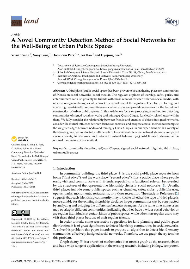
Citation: Yang, Y.; Peng, S.; Park,

D.-S.; Hao, F.; Lee, H. A Novel

Community Detection Method of

Social Networks for the Well-Being of

Urban Public Spaces. Land 2022, 11,

716. https://doi.org/10.3390/

land11050716

Academic Editor: Jun-Ho Huh

Received: 31 March 2022

Accepted: 7 May 2022

Published: 10 May 2022

Publisher’s Note: MDPI stays neutral

with regard to jurisdictional claims in

published maps and institutional affil-

iations.

Copyright: © 2022 by the authors.

Licensee MDPI, Basel, Switzerland.

This article is an open access article

distributed under the terms and

conditions of the Creative Commons

Attribution (CC BY) license (https://

creativecommons.org/licenses/by/

4.0/).

land

Article

A Novel Community Detection Method of Social Networks forthe Well-Being of Urban Public SpacesYixuan Yang 1, Sony Peng 1, Doo-Soon Park 1,*, Fei Hao 2 and Hyejung Lee 3

1 Department of Software Convergence, Soonchunhyang University,Asan-si 31538, Chungcheongnam-do, Korea; yangyixuan@sch.ac.kr (Y.Y.); sony@sch.ac.kr (S.P.)

2 School of Computer Science, Shaanxi Normal University, Xi’an 710119, China; fhao@snnu.edu.cn3 Institute for Artificial Intelligence and Software, Soonchunhyang University,

Asan-si 31538, Chungcheongnam-do, Korea; hjlee100@sch.ac.kr* Correspondence: parkds@sch.ac.kr; Tel.: +82-41-530-1317; Fax: +82-41-530-1548

Abstract: A third place (public social space) has been proven to be a gathering place for communitiesof friends on social networks (social media). The regulars at places of worship, cafes, parks, andentertainment can also possibly be friends with those who follow each other on social media, withother non-regulars being social network friends of one of the regulars. Therefore, detecting andanalyzing user-friendly communities on social networks can provide references for the layout andconstruction of urban public spaces. In this article, we focus on proposing a method for detectingcommunities of signed social networks and mining γ-Quasi-Cliques for closely related users withinthem. We fully consider the relationship between friends and enemies of objects in signed networks,consider the mutual influence between friends or enemies, and propose a novel method to recomputethe weighted edges between nodes and mining γ-Quasi-Cliques. In our experiment, with a variety ofthresholds given, we conducted multiple sets of tests via real-life social network datasets, comparedvarious reweighted datasets, and detected maximal balanced γ-Quasi-Cliques to determine theoptimal parameters of our method.

Keywords: community detection; γ-Quasi-Cliques; signed social network; big data; third place;urban public spaces

1. Introduction

In community building, the third place [1] is the social public place separate fromhome (“first place”) and the workplace (“second place”). It is a public place where peopleeasily visit and communicate with friends; especially, its functional role can be revealedby the structures of the representative friendship circles in social networks [2]. Usually,third places include some public spaces such as churches, cafes, clubs, public libraries,operas, parks, monuments, restaurants, or indoor recreation. The study in Reference [2]suggests that each friendship community may indicate whether the type of third place ismore suitable for the existing friendship circle, or larger communities can be constructedby analyzing and bridging the differences between strangers. At the same time, some usersmay overlap in different communities, indicating that they have a wider social behavior orare regular individuals in certain kinds of public spaces, while other non-regular users mayvisit these third places because of their regular friends.

In order to make some reasonable suggestions for land planning and public spacedistribution, it is of great significance to detect friendship communities in social networks.To solve this problem, this paper intends to propose an algorithm to detect friend/enemycommunities effectively in signed social networks. Therefore, we use graph theory to solvethis problem.

Graph theory [3] is a branch of mathematics that treats a graph as the research objectand has a wide range of applications in the existing research, including biology, computers,

Land 2022, 11, 716. https://doi.org/10.3390/land11050716 https://www.mdpi.com/journal/land

Land 2022, 11, 716 2 of 16

social systems, and other fields such as protein interaction network analysis, genetic biologynetwork analysis, web community mining, social network analysis, and knowledge graphconstruction [4,5]. In addition, recently, the graph mining technique in the social networkhas been considered as an important research direction in the data field. A graph in graphtheory is composed of several given nodes and edges, and the edges connect certain nodes.A graph is usually used to describe the specific relationship between particular objects. Forexample, a node is used to represent a user in the social network; an edge is utilized toconnect two users, indicating a relationship between the corresponding ones.

Typically, nodes in a network represent individuals, while edges represent the relation-ships between them. In the regular setting, only positive relations representing proximityor similarity are considered. However, when the network has like/dislike, love/hate, re-spect/disrespect, or trust/distrust relationships, such a representation, with only a positiveedge, is not enough, since it cannot encode the sign of the relationship. These networks canbe modeled as the signed social networks, where edge weights can be positive or negative.Early use of signed networks can be found in anthropology, where negative edges wereused to represent antagonistic relationships between tribes. In earlier years, signed socialnetworks were used in anthropology, where negative edges were used to denote negativerelations such as tribal hostility [6]. In the field of computer science, there is a lot of researchon signed social networks, for example, Silviu built a signed network for Wikipedia [7],Liu et al. Al proposed a link prediction method for a signed social network [8], and Timopresented a model for creating signed networks enabling friends profit from enemies [9].

The most common theory associated with signed social networks is the “social balancetheory”, which intuitively can be interpreted as “my friend’s friend is my friend”, “myfriend’s enemy is my enemy”, “my enemy’s friend is my enemy”, and “my enemy’s enemyis my friend”. Below, we present a definition, in that a graph is balanced if any part of thegraph does not conflict with the “social balance theory”.

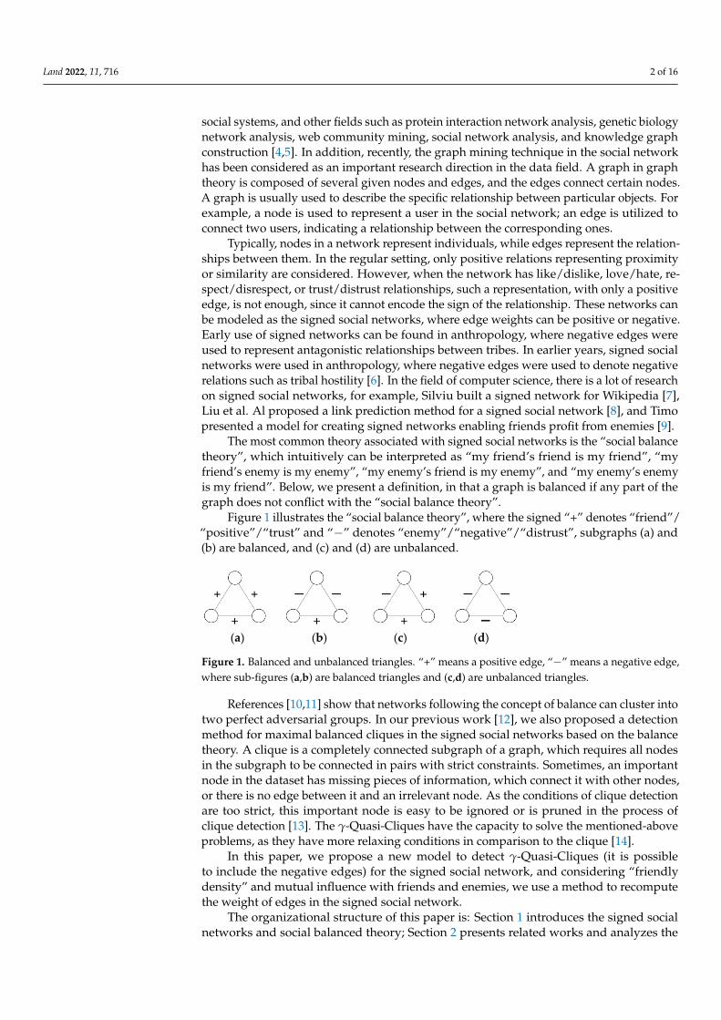
Figure 1 illustrates the “social balance theory”, where the signed “+” denotes “friend”/“positive”/“trust” and “−” denotes “enemy”/“negative”/“distrust”, subgraphs (a) and(b) are balanced, and (c) and (d) are unbalanced.

Land 2022, 11, x FOR PEER REVIEW 2 of 16

Graph theory [3] is a branch of mathematics that treats a graph as the research object and has a wide range of applications in the existing research, including biology, comput-ers, social systems, and other fields such as protein interaction network analysis, genetic biology network analysis, web community mining, social network analysis, and knowledge graph construction [4,5]. In addition, recently, the graph mining technique in the social network has been considered as an important research direction in the data field. A graph in graph theory is composed of several given nodes and edges, and the edges connect certain nodes. A graph is usually used to describe the specific relationship be-tween particular objects. For example, a node is used to represent a user in the social net-work; an edge is utilized to connect two users, indicating a relationship between the cor-responding ones.

Typically, nodes in a network represent individuals, while edges represent the rela-tionships between them. In the regular setting, only positive relations representing prox-imity or similarity are considered. However, when the network has like/dislike, love/hate, respect/disrespect, or trust/distrust relationships, such a representation, with only a posi-tive edge, is not enough, since it cannot encode the sign of the relationship. These net-works can be modeled as the signed social networks, where edge weights can be positive or negative. Early use of signed networks can be found in anthropology, where negative edges were used to represent antagonistic relationships between tribes. In earlier years, signed social networks were used in anthropology, where negative edges were used to denote negative relations such as tribal hostility [6]. In the field of computer science, there is a lot of research on signed social networks, for example, Silviu built a signed network for Wikipedia [7], Liu et al. Al proposed a link prediction method for a signed social net-work [8], and Timo presented a model for creating signed networks enabling friends profit from enemies [9].

The most common theory associated with signed social networks is the “social bal-ance theory”, which intuitively can be interpreted as “my friend’s friend is my friend”, “my friend’s enemy is my enemy”, “my enemy’s friend is my enemy”, and “my enemy’s enemy is my friend”. Below, we present a definition, in that a graph is balanced if any part of the graph does not conflict with the “social balance theory”.

Figure 1 illustrates the “social balance theory”, where the signed “+” denotes “friend”/“positive”/“trust” and “−” denotes “enemy”/“negative”/“distrust”, subgraphs (a) and (b) are balanced, and (c) and (d) are unbalanced.

(a) (b) (c) (d)

Figure 1. Balanced and unbalanced triangles. “+” means a positive edge, “−” means a negative edge, where sub-figures (a,b) are balanced triangles and (c,d) are unbalanced triangles.

References [10,11] show that networks following the concept of balance can cluster into two perfect adversarial groups. In our previous work [12], we also proposed a detec-tion method for maximal balanced cliques in the signed social networks based on the bal-ance theory. A clique is a completely connected subgraph of a graph, which requires all nodes in the subgraph to be connected in pairs with strict constraints. Sometimes, an im-portant node in the dataset has missing pieces of information, which connect it with other nodes, or there is no edge between it and an irrelevant node. As the conditions of clique detection are too strict, this important node is easy to be ignored or is pruned in the pro-cess of clique detection [13]. The 𝛾-Quasi-Cliques have the capacity to solve the men-tioned-above problems, as they have more relaxing conditions in comparison to the clique [14].

Figure 1. Balanced and unbalanced triangles. “+” means a positive edge, “−” means a negative edge,where sub-figures (a,b) are balanced triangles and (c,d) are unbalanced triangles.

References [10,11] show that networks following the concept of balance can cluster intotwo perfect adversarial groups. In our previous work [12], we also proposed a detectionmethod for maximal balanced cliques in the signed social networks based on the balancetheory. A clique is a completely connected subgraph of a graph, which requires all nodesin the subgraph to be connected in pairs with strict constraints. Sometimes, an importantnode in the dataset has missing pieces of information, which connect it with other nodes,or there is no edge between it and an irrelevant node. As the conditions of clique detectionare too strict, this important node is easy to be ignored or is pruned in the process ofclique detection [13]. The γ-Quasi-Cliques have the capacity to solve the mentioned-aboveproblems, as they have more relaxing conditions in comparison to the clique [14].

In this paper, we propose a new model to detect γ-Quasi-Cliques (it is possibleto include the negative edges) for the signed social network, and considering “friendlydensity” and mutual influence with friends and enemies, we use a method to recomputethe weight of edges in the signed social network.

The organizational structure of this paper is: Section 1 introduces the signed socialnetworks and social balanced theory; Section 2 presents related works and analyzes the

Land 2022, 11, 716 3 of 16

clustering method for the signed social network in the existing research work; Section 3explains the basic knowledge about the “friendly density theory” and signed social networkand introduces a way to recompute the weight of edges in the signed network and themaximal balanced γ-Quasi-Clique detect method; Section 4 applies the famous opendatasets on our model in the experiment, and determines the optimal threshold for filteringthe recomputed weight adjacency matrix and the best value of γ. Finally, Section 5 presentsthe conclusion of the work and further stages of the research.

2. Related Works

Signed social networks with positive and negative links have attracted considerableattention over the past few years. One of the main challenges in signed network analysis iscommunity detection, which aims to find mutually opposing groups with two character-istics: (1) entities within the same group have as many positive relationships as possible;(2) entities between different groups have as many negative relationships as possible.

The majority of existing algorithms for community detection in signed networks aimto provide hard partitioning of the network, where any node should belong to a singlecommunity, such as cliques [15]. However, overlapping communities, in which a node isallowed to belong to multiple communities, are widespread in many real-world networks.Another disadvantage of some existing algorithms is that the final number of clusters kshould be the input to the clustering process. However, it may be the case that we do notknow k in advance. It will have the limitation of detecting communities by giving clustersthe number k.

However, the clustering algorithm of a signed social network cannot succeed to obtainthe results only by directly extending the theory and algorithm of the unsigned socialnetwork. When edge weights are allowed to be negative, many unsigned social networkconcepts and algorithms collapse, because they do not work properly in this situation.More recently, studies have been conducted to develop algorithms for efficient methodsof clustering signed networks. Doreian and Mrvar [16] proposed a local search strategysimilar to Kernighan-Lin algorithm. Yang et al. [17] proposed an agent-based approach,which is essentially a random walk on a graph. Anchuri and Magdon-Ismail1 proposed ahierarchical iterative approach to solve two-way frustrations and signed modularity usingspectrum relaxation targets at each level. Bansal et al. [18] also considered the problem ofsigned graph clustering, although their formula is driven by correlation clustering. Theyproposed two approximation algorithms and proved the approximation bounds.

Renjie et al. [19] proposed a model, named stable k-core, to measure the stability of acommunity in signed graphs. Chengyi et al. [20] gave an improved modularity functionfor signed networks on the basis of the existing modularity function and devised a newcommunity detection algorithm for signed networks. Cadena et al. [21] extended theconcept of subgraph density to detect events in signed networks. Ref. [22] is devoted tothe study of influence diffusion in signed networks and studies the process of influencediffusion in signed networks. In [23], Tsourakakis et al. considered dense graph detectionproblems with negative weights. Ordozgoiti et al. [24] proposed a more efficient andscalable approach to this problem.

Qi et al. [25] proposed a framework to solve the problem of negative weights in thesigned social networks. In the first step, the authors defined a new computation processto compute the weights between two nodes. They combined the negative edges with thepositive ones directly into a parameter called “friendly density”. The proposal of thisdefinition becomes a great contribution to the more objective and reasonable recomputationof edge weights. This paper refers to the definition of friend density to recompute theweights of edges in the next section. Moreover, utilizing the mentioned definition, weconsider the six-dimensional space theory [26] to further reasonably compute and obtain anew weight adjacency matrix.

Land 2022, 11, 716 4 of 16

3. Basic Notions and Approach3.1. Terminologies and Notations3.1.1. Recalculate the Weights between Friends

A signed social network graph can be noted as G = (V, E, W), where V is a set of nodes,E is a set of weights edges that represents the relationships between the nodes, W is theweight on every edge e, the adjacency matrix A is defined as follows:

A =

|w(e)|, i f e

(vi, vj

)is positive

−|w(e)|, i f e(vi, vj

)is negative

0, i f(vi, vj

)is unknown

(1)

For a network G with only positive edges, clustering can be seen as a process thatdetects all dense subgraphs in G [25]. The computation of dense subgraph C is defined by:

d(G′)=

2 ∑e∈E(G′) w(e)|V(G′)||V(G′)− 1| . (2)

When the G’ is a subgraph of G, w(e) is the weight of edge e in E(G’), |·| is theabsolute value of the number. Equation (2) can be generalized to a singed graph wherew(e) can be negative. The density of the graph will drop or rise by adding new negative orpositive edges.

In a signed network, the relationship between two nodes (i.e., the weights of theedges) may be influenced by rumors/personal bias and may be negative and close to 0,and that negative relationship is subjective and one-sided. When both nodes have positiverelationships with their mutual friends, that negative edge is easily influenced by themutual influence of the friends’ positive relationship. In order to avoid such assertivepositive/negative edges caused by considering only the relationship between two nodes,and to better cluster the friendly density clusters, we plan to consider the true state oftwo nodes based on a more “global” structural environment and adjust their pre-existingor given relationships as necessary. Therefore, we recalculate the relationship weightsbetween two nodes considering the global structural environment and redefine theirpositive/negative relationship by a reasonable threshold (the selection of the thresholdis explored in Section 4 in order not to destroy the original network structure as muchas possible).

To solve this problem, reference [25] introduces a weight-completing method, accord-ing to which we will obtain the different weights βζ based on length ζ of the path Pζ .

wu,v =k

∑ζ=1

[βζ ∗ ∑PεPζ

∏eεP

w(e)] (3)

Among them, ζ represents the path length, k is the maximum value of the path lengthζ, the formula traverses all paths of the path length ζ ∈ [1, k], and for each path P, themultiplication of the weights wu,v of each edge e on the path P is calculated. If there aremultiple paths P of the same length ζ, find the sum of their concatenated products.

Figure 2 shows an example to explain it. There are three paths between nodes u andv, and the value of each edge represents the positive/negative relationship and weightbetween the two nodes. When we consider each path equally, βζ = 1, and according toEquation (3), the predicted weight of wu,v is

wu,v = 0.3− 0.5× 0.1− 0.5× 0.3× 0.1 = 0.235

Land 2022, 11, 716 5 of 16

Land 2022, 11, x FOR PEER REVIEW 5 of 16

If we use the decaying function 𝛽 = !, then the predicted weight of 𝑤 , is

𝑤 , = 0.3 − 0.5 × 0.12! − 0.5 × 0.3 × 0.13! = 0.2725

Figure 2. Completing the weight between u and v.

Comparing the two 𝑤 , , when we choose decaying function 𝛽 = !, the positive re-lationship between u and v becomes more evident. Similarly, through the calculation of Equation (3), the weight of the negative edge may be more negative.

We give an example below to calculate the new relationship value under the mutual influences of common friends even if the direct relationship between nodes u and v is negative, taking into account reasons such as rumors or personal biases: even their direct relationship is negative, and they should gather together in the same cluster. In the exam-ple, we choose 𝛽 = ! 𝑎𝑠 𝑡ℎ𝑒 decaying function. The original graph of this example is shown as Figure 3.

Example:

Figure 3. The original graph g.

𝑤 , = −0.1 + 0.4 × 0.82! − 0.7 × 0.92! = 0.375

After recalculating the weights between nodes u, v, the network is updated to Figure 4. It is obvious that the network becomes a balanced network, which can be detected in the next step of the balanced community detection algorithm. At this time, the relationship between u and v changes from negative to positive, which is an important reason to use common friends/enemies as parameters for weight calculation. This step can as far as pos-sible avoid the influence of rumors, personal biases, or noisy data collection, and is more comprehensive consider the relationship between two nodes.

Figure 2. Completing the weight between u and v.

If we use the decaying function βζ = 1ζ! , then the predicted weight of wu,v is

wu,v = 0.3− 0.5× 0.12!

− 0.5× 0.3× 0.13!

= 0.2725

Comparing the two wu,v, when we choose decaying function βζ = 1ζ! , the positive

relationship between u and v becomes more evident. Similarly, through the calculation ofEquation (3), the weight of the negative edge may be more negative.

We give an example below to calculate the new relationship value under the mutualinfluences of common friends even if the direct relationship between nodes u and v isnegative, taking into account reasons such as rumors or personal biases: even their directrelationship is negative, and they should gather together in the same cluster. In the example,we choose βζ = 1

ζ! as the decaying function. The original graph of this example is shown asFigure 3.

Land 2022, 11, x FOR PEER REVIEW 5 of 16

If we use the decaying function 𝛽 = !, then the predicted weight of 𝑤 , is

𝑤 , = 0.3 − 0.5 × 0.12! − 0.5 × 0.3 × 0.13! = 0.2725

Figure 2. Completing the weight between u and v.

Comparing the two 𝑤 , , when we choose decaying function 𝛽 = !, the positive re-lationship between u and v becomes more evident. Similarly, through the calculation of Equation (3), the weight of the negative edge may be more negative.

We give an example below to calculate the new relationship value under the mutual influences of common friends even if the direct relationship between nodes u and v is negative, taking into account reasons such as rumors or personal biases: even their direct relationship is negative, and they should gather together in the same cluster. In the exam-ple, we choose 𝛽 = ! 𝑎𝑠 𝑡ℎ𝑒 decaying function. The original graph of this example is shown as Figure 3.

Example:

Figure 3. The original graph g.

𝑤 , = −0.1 + 0.4 × 0.82! − 0.7 × 0.92! = 0.375

After recalculating the weights between nodes u, v, the network is updated to Figure 4. It is obvious that the network becomes a balanced network, which can be detected in the next step of the balanced community detection algorithm. At this time, the relationship between u and v changes from negative to positive, which is an important reason to use common friends/enemies as parameters for weight calculation. This step can as far as pos-sible avoid the influence of rumors, personal biases, or noisy data collection, and is more comprehensive consider the relationship between two nodes.

Figure 3. The original graph g.

Example:

wu,v = −0.1 +0.4× 0.8

2!− 0.7× 0.9

2!= 0.375

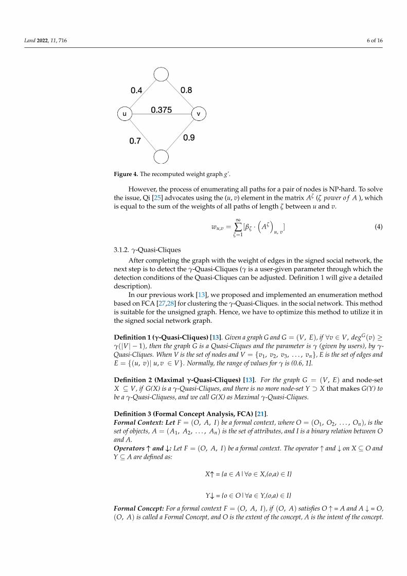
After recalculating the weights between nodes u, v, the network is updated to Figure 4.It is obvious that the network becomes a balanced network, which can be detected in thenext step of the balanced community detection algorithm. At this time, the relationshipbetween u and v changes from negative to positive, which is an important reason to usecommon friends/enemies as parameters for weight calculation. This step can as far aspossible avoid the influence of rumors, personal biases, or noisy data collection, and ismore comprehensive consider the relationship between two nodes.

Land 2022, 11, 716 6 of 16Land 2022, 11, x FOR PEER REVIEW 6 of 16

Figure 4. The recomputed weight graph g’.

However, the process of enumerating all paths for a pair of nodes is NP-hard. To solve the issue, Qi [25] advocates using the (u, v) element in the matrix 𝐴 (𝜁 𝑝𝑜𝑤𝑒𝑟 𝑜𝑓 𝐴 ), which is equal to the sum of the weights of all paths of length 𝜁 between u and v.

𝑤 , = [𝛽 ⋅ (𝐴 ) , ] (4)

3.1.2. 𝛾-Quasi-Cliques After completing the graph with the weight of edges in the signed social network,

the next step is to detect the 𝛾-Quasi-Cliques (𝛾 is a user-given parameter through which the detection conditions of the Quasi-Cliques can be adjusted. Definition 1 will give a de-tailed description).

In our previous work [13], we proposed and implemented an enumeration method based on FCA [27,28] for clustering the 𝛾 -Quasi-Cliques. in the social network. This method is suitable for the unsigned graph. Hence, we have to optimize this method to utilize it in the signed social network graph.

Definition 1 (𝜸-Quasi-Cliques) [13]. Given a graph G and 𝐺 = (𝑉, 𝐸), if∀𝑣 ∈ 𝑉, 𝑑𝑒𝑔 (𝑣) ≥ 𝛾(|𝑉| − 1), then the graph G is a Quasi-Cliques and the parameter is 𝛾 (given by users), by 𝛾-Quasi-Cliques. When V is the set of nodes and 𝑉 = {𝑣 , 𝑣 , 𝑣 , … , 𝑣 }, E is the set of edges and 𝐸 ={(𝑢, 𝑣)| 𝑢, 𝑣 ∈ 𝑉}. Normally, the range of values for 𝛾 is (0.6, 1].

Definition 2 (Maximal 𝜸-Quasi-Cliques) [13]. For the graph 𝐺 = (𝑉, 𝐸) and node-set 𝑋 ⊆ 𝑉, if G(X) is a 𝛾-Quasi-Cliques, and there is no more node-set 𝑌 ⊃ 𝑋 that makes G(Y) to be a 𝛾-Quasi-Cliquess, and we call G(X) as Maximal 𝛾-Quasi-Cliques.

Definition 3 (Formal Concept Analysis, FCA) [21]. Formal Context: Let 𝐹 = (𝑂, 𝐴, 𝐼) be a formal context, where 𝑂 = (𝑂 , 𝑂 , … , 𝑂 ), is the set of objects, 𝐴 = (𝐴 , 𝐴 , … , 𝐴 ) is the set of attributes, and I is a binary relation between O and A. Operators↑ and ↓: Let 𝐹 = (𝑂, 𝐴, 𝐼) be a formal context. The operator ↑ and ↓ on X ⊆ O and Y ⊆ A are defined as:

X↑ = {a ∈ A|∀o ∈ X,(o,a) ∈ I}

Y↓ = {o ∈ O|∀a ∈ Y,(o,a) ∈ I}

Formal Concept: For a formal context 𝐹 = (𝑂, 𝐴, 𝐼), if (𝑂, 𝐴) satisfies O↑ = A and A↓ = O, (𝑂, 𝐴) is called a Formal Concept, and O is the extent of the concept, A is the intent of the concept. All formal concepts form the formal concept lattice by the partial relation are as (O1, A1) ≤ (O2, A2) ↔ O1 ⊆ O2(↔ A1 ⊇ A2).

Figure 4. The recomputed weight graph g’.

However, the process of enumerating all paths for a pair of nodes is NP-hard. To solvethe issue, Qi [25] advocates using the (u, v) element in the matrix Aζ (ζ power o f A ), whichis equal to the sum of the weights of all paths of length ζ between u and v.

wu,v =∞

∑ζ=1

[βζ ·(

Aζ)

u, v] (4)

3.1.2. γ-Quasi-Cliques

After completing the graph with the weight of edges in the signed social network, thenext step is to detect the γ-Quasi-Cliques (γ is a user-given parameter through which thedetection conditions of the Quasi-Cliques can be adjusted. Definition 1 will give a detaileddescription).

In our previous work [13], we proposed and implemented an enumeration methodbased on FCA [27,28] for clustering the γ-Quasi-Cliques. in the social network. This methodis suitable for the unsigned graph. Hence, we have to optimize this method to utilize it inthe signed social network graph.

Definition 1 (γ-Quasi-Cliques) [13]. Given a graph G and G = (V, E), if ∀v ∈ V, degG(v) ≥γ(|V| − 1), then the graph G is a Quasi-Cliques and the parameter is γ (given by users), by γ-Quasi-Cliques. When V is the set of nodes and V = {v1, v2, v3, . . . , vn}, E is the set of edges andE = {(u, v)| u, v ∈ V}. Normally, the range of values for γ is (0.6, 1].

Definition 2 (Maximal γ-Quasi-Cliques) [13]. For the graph G = (V, E) and node-setX ⊆ V, if G(X) is a γ-Quasi-Cliques, and there is no more node-set Y ⊃ X that makes G(Y) tobe a γ-Quasi-Cliquess, and we call G(X) as Maximal γ-Quasi-Cliques.

Definition 3 (Formal Concept Analysis, FCA) [21].Formal Context: Let F = (O, A, I) be a formal context, where O = (O1, O2, . . . , On), is theset of objects, A = (A1, A2, . . . , An) is the set of attributes, and I is a binary relation between Oand A.Operators ↑ and ↓: Let F = (O, A, I) be a formal context. The operator ↑ and ↓ on X ⊆ O andY ⊆ A are defined as:

X↑ = {a ∈ A|∀o ∈ X,(o,a) ∈ I}

Y↓ = {o ∈ O|∀a ∈ Y,(o,a) ∈ I}

Formal Concept: For a formal context F = (O, A, I), if (O, A) satisfies O ↑ = A and A ↓ = O,(O, A) is called a Formal Concept, and O is the extent of the concept, A is the intent of the concept.

Land 2022, 11, 716 7 of 16

All formal concepts form the formal concept lattice by the partial relation are as (O1, A1) ≤ (O2, A2)

Land 2022, 11, x FOR PEER REVIEW 6 of 16

Figure 4. The recomputed weight graph g’.

However, the process of enumerating all paths for a pair of nodes is NP-hard. To solve the issue, Qi [25] advocates using the (u, v) element in the matrix 𝐴 (𝜁 𝑝𝑜𝑤𝑒𝑟 𝑜𝑓 𝐴 ), which is equal to the sum of the weights of all paths of length 𝜁 between u and v.

𝑤 , = [𝛽 ⋅ (𝐴 ) , ] (4)

3.1.2. 𝛾-Quasi-Cliques After completing the graph with the weight of edges in the signed social network,

the next step is to detect the 𝛾-Quasi-Cliques (𝛾 is a user-given parameter through which the detection conditions of the Quasi-Cliques can be adjusted. Definition 1 will give a de-tailed description).

In our previous work [13], we proposed and implemented an enumeration method based on FCA [27,28] for clustering the 𝛾 -Quasi-Cliques. in the social network. This method is suitable for the unsigned graph. Hence, we have to optimize this method to utilize it in the signed social network graph.

Definition 1 (𝜸-Quasi-Cliques) [13]. Given a graph G and 𝐺 = (𝑉, 𝐸), if∀𝑣 ∈ 𝑉, 𝑑𝑒𝑔 (𝑣) ≥ 𝛾(|𝑉| − 1), then the graph G is a Quasi-Cliques and the parameter is 𝛾 (given by users), by 𝛾-Quasi-Cliques. When V is the set of nodes and 𝑉 = {𝑣 , 𝑣 , 𝑣 , … , 𝑣 }, E is the set of edges and 𝐸 ={(𝑢, 𝑣)| 𝑢, 𝑣 ∈ 𝑉}. Normally, the range of values for 𝛾 is (0.6, 1].

Definition 2 (Maximal 𝜸-Quasi-Cliques) [13]. For the graph 𝐺 = (𝑉, 𝐸) and node-set 𝑋 ⊆ 𝑉, if G(X) is a 𝛾-Quasi-Cliques, and there is no more node-set 𝑌 ⊃ 𝑋 that makes G(Y) to be a 𝛾-Quasi-Cliquess, and we call G(X) as Maximal 𝛾-Quasi-Cliques.

Definition 3 (Formal Concept Analysis, FCA) [21]. Formal Context: Let 𝐹 = (𝑂, 𝐴, 𝐼) be a formal context, where 𝑂 = (𝑂 , 𝑂 , … , 𝑂 ), is the set of objects, 𝐴 = (𝐴 , 𝐴 , … , 𝐴 ) is the set of attributes, and I is a binary relation between O and A. Operators↑ and ↓: Let 𝐹 = (𝑂, 𝐴, 𝐼) be a formal context. The operator ↑ and ↓ on X ⊆ O and Y ⊆ A are defined as:

X↑ = {a ∈ A|∀o ∈ X,(o,a) ∈ I}

Y↓ = {o ∈ O|∀a ∈ Y,(o,a) ∈ I}

Formal Concept: For a formal context 𝐹 = (𝑂, 𝐴, 𝐼), if (𝑂, 𝐴) satisfies O↑ = A and A↓ = O, (𝑂, 𝐴) is called a Formal Concept, and O is the extent of the concept, A is the intent of the concept. All formal concepts form the formal concept lattice by the partial relation are as (O1, A1) ≤ (O2, A2) ↔ O1 ⊆ O2(↔ A1 ⊇ A2). O1 ⊆ O2(

Land 2022, 11, x FOR PEER REVIEW 6 of 16

Figure 4. The recomputed weight graph g’.

However, the process of enumerating all paths for a pair of nodes is NP-hard. To solve the issue, Qi [25] advocates using the (u, v) element in the matrix 𝐴 (𝜁 𝑝𝑜𝑤𝑒𝑟 𝑜𝑓 𝐴 ), which is equal to the sum of the weights of all paths of length 𝜁 between u and v.

𝑤 , = [𝛽 ⋅ (𝐴 ) , ] (4)

3.1.2. 𝛾-Quasi-Cliques After completing the graph with the weight of edges in the signed social network,

the next step is to detect the 𝛾-Quasi-Cliques (𝛾 is a user-given parameter through which the detection conditions of the Quasi-Cliques can be adjusted. Definition 1 will give a de-tailed description).

In our previous work [13], we proposed and implemented an enumeration method based on FCA [27,28] for clustering the 𝛾 -Quasi-Cliques. in the social network. This method is suitable for the unsigned graph. Hence, we have to optimize this method to utilize it in the signed social network graph.

Definition 1 (𝜸-Quasi-Cliques) [13]. Given a graph G and 𝐺 = (𝑉, 𝐸), if∀𝑣 ∈ 𝑉, 𝑑𝑒𝑔 (𝑣) ≥ 𝛾(|𝑉| − 1), then the graph G is a Quasi-Cliques and the parameter is 𝛾 (given by users), by 𝛾-Quasi-Cliques. When V is the set of nodes and 𝑉 = {𝑣 , 𝑣 , 𝑣 , … , 𝑣 }, E is the set of edges and 𝐸 ={(𝑢, 𝑣)| 𝑢, 𝑣 ∈ 𝑉}. Normally, the range of values for 𝛾 is (0.6, 1].

Definition 2 (Maximal 𝜸-Quasi-Cliques) [13]. For the graph 𝐺 = (𝑉, 𝐸) and node-set 𝑋 ⊆ 𝑉, if G(X) is a 𝛾-Quasi-Cliques, and there is no more node-set 𝑌 ⊃ 𝑋 that makes G(Y) to be a 𝛾-Quasi-Cliquess, and we call G(X) as Maximal 𝛾-Quasi-Cliques.

Definition 3 (Formal Concept Analysis, FCA) [21]. Formal Context: Let 𝐹 = (𝑂, 𝐴, 𝐼) be a formal context, where 𝑂 = (𝑂 , 𝑂 , … , 𝑂 ), is the set of objects, 𝐴 = (𝐴 , 𝐴 , … , 𝐴 ) is the set of attributes, and I is a binary relation between O and A. Operators↑ and ↓: Let 𝐹 = (𝑂, 𝐴, 𝐼) be a formal context. The operator ↑ and ↓ on X ⊆ O and Y ⊆ A are defined as:

X↑ = {a ∈ A|∀o ∈ X,(o,a) ∈ I}

Y↓ = {o ∈ O|∀a ∈ Y,(o,a) ∈ I}

Formal Concept: For a formal context 𝐹 = (𝑂, 𝐴, 𝐼), if (𝑂, 𝐴) satisfies O↑ = A and A↓ = O, (𝑂, 𝐴) is called a Formal Concept, and O is the extent of the concept, A is the intent of the concept. All formal concepts form the formal concept lattice by the partial relation are as (O1, A1) ≤ (O2, A2) ↔ O1 ⊆ O2(↔ A1 ⊇ A2). A1 ⊇ A2).

In our early work [13], we proved that according to calculating and utilizing the extentor intent of the concept in the formal concept lattice, we can obtain the node number ineach γ-Quasi-Cliques, and then we can calculate the degree in each γ-Quasi-Cliques anddetermine whether it satisfies degG(V) ≥ γ(|V| − 1) (refer to Definition 1). This process isrepresented by pseudocode as Algorithm 1:

Algorithm 1 γ-Quasi-Cliques Detection

1 : Input γ, formal context f2: begin3: Formal Concept Lattice← Construct FCA(f )4: for each concept ∈ Formal Concept Lattice:5: value← γ * concept.extent.length6: flag← True7: degree← degree(all nodes of concept)8: if value > degree:9: flag = False10: if flag is True:11: QuasiCliques.add(concept)12: return QuasiCliques13: End

3.2. Methodology of Maximal Balanced γ-Quasi-Cliques Detection3.2.1. Overview

In this subsection, we present the overall framework of the methodology of this paper,shown as Figure 5. The method in this paper is able to be divided into three steps: considerthe mutual influence between nodes, re-compute the weights of the edges; generate positive,negative and weightless matrices, and obtain the corresponding Quasi-Cliques, namelyQC(AMP), QC(AMN) and QC(AMT); detect maximal balanced γ-Quasi-Cliques.

 

 

 

 Land 2022, 11, x. https://doi.org/10.3390/xxxxx  www.mdpi.com/journal/land 

 

 

Figure 5. The overview of our method.

Land 2022, 11, 716 8 of 16

3.2.2. Optimization of Weight Matrix Computation

As the value of length ζ in Equation (4) is ζ ∈ [1, ∞), a large amount of calculationswill still be generated when βζ = 1

ζ! gradually approaches 0 (ζ goes to in f inity); thus, areasonable maximum length ζ is selected in this paper. As mentioned in Section 2, afterreferring to the six-dimensional space theory, we only focus on all paths with a path lengthζ less than or equal to 6, while choosing the decaying function βζ = 1

ζ! , we receive theweight of (u, v) equal to:

wu,v =6

∑ζ=1

[1ζ!·(

Aζ)

u, v=

(I + A +

A2

2!+

A3

3!+

A4

4!+

A5

5!+

A6

6!

). (5)

Since most large social networks are sparse graphs [29], when performing matrixexponentiation on a large social network, we can consider a variety of existing sparse matrixexponentiation methods to improve computational efficiency, e.g., fast exponentiationfor matrices [30], which leverage the paradigm to process exponentiation in parallel onGPUs [31]. At the same time, in this paper, we only focus on the first 6th power operationof the matrix instead of the high-power operation. Compared with Equation (4), thecomplexity of the matrix power operation in this paper is not high.

3.2.2.1. Our Maximal Balanced γ-Quasi-Cliques Detection Method

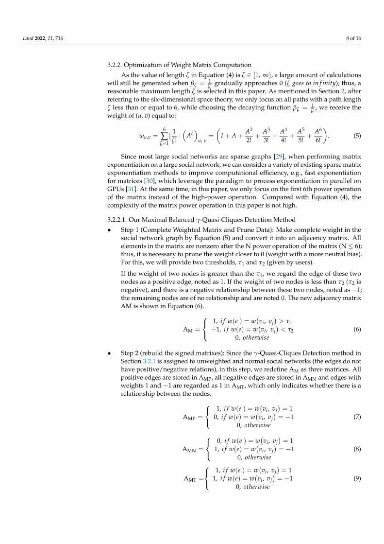
• Step 1 (Complete Weighted Matrix and Prune Data): Make complete weight in thesocial network graph by Equation (5) and convert it into an adjacency matrix. Allelements in the matrix are nonzero after the N power operation of the matrix (N ≤ 6);thus, it is necessary to prune the weight closer to 0 (weight with a more neutral bias).For this, we will provide two thresholds, τ1 and τ2 (given by users).

If the weight of two nodes is greater than the τ1, we regard the edge of these twonodes as a positive edge, noted as 1. If the weight of two nodes is less than τ2 (τ2 isnegative), and there is a negative relationship between these two nodes, noted as −1;the remaining nodes are of no relationship and are noted 0. The new adjacency matrixAM is shown in Equation (6).

AM =

1, i f w(e ) = w

(vi, vj

)> τ1

−1, i f w(e) = w(vi, vj

)< τ2

0, otherwise(6)

• Step 2 (rebuild the signed matrixes): Since the γ-Quasi-Cliques Detection method inSection 3.2.1 is assigned to unweighted and normal social networks (the edges do nothave positive/negative relations), in this step, we redefine AM as three matrices. Allpositive edges are stored in AMP, all negative edges are stored in AMN and edges withweights 1 and −1 are regarded as 1 in AMT, which only indicates whether there is arelationship between the nodes.

AMP =

1, i f w(e ) = w

(vi, vj

)= 1

0, i f w(e) = w(vi, vj

)= −1

0, otherwise(7)

AMN =

0, i f w(e ) = w

(vi, vj

)= 1

1, i f w(e) = w(vi, vj

)= −1

0, otherwise(8)

AMT =

1, i f w(e ) = w

(vi, vj

)= 1

1, i f w(e) = w(vi, vj

)= −1

0, otherwise(9)

Land 2022, 11, 716 9 of 16

• Step 3 (γ-Quasi-Cliques Detection): Using these three matrixes as input values, per-form Quasi-cluster detection to obtain Quasi-Cliques sets QC(AMT), QC(AMP), andQC(AMN), if the Quasi-Cliques in quasi-clusters QC(AMP) and QC(AMN) exist inQC(AMT), then they are our final output: Signed γ-Quasi-Cliques.

Notes: The QC(AMP) is the set of γ-Quasi-Cliques with positive edges, theQC(AMN) is the set of γ-Quasi-Cliques with negative edges, the QC(AMT) is theset of γ-Quasi-Cliques with positive edges and negative edges (regardless of thesign of the edges). If the γ-Quasi-Clique E1 and γ-Quasi-Clique E2 are both inthe QC(AMP), there are positive relationships among the nodes in E1 and E2, re-spectively, the E1 and E2 form a γ-Quasi-Clique in QC(AMN), and there are neg-ative relationships among the nodes in merger set of E1 and E2. Meanwhile, themerger set of E1 and E2 with positive and negative edges is a γ-Quasi-Clique inQC(AMT), which means that all nodes in E1 and E2 can form a γ-Quasi-Clique.At this point, this γ-Quasi-Clique is a maximal balanced γ-Quasi-Clique.

To explain the above notes more intuitively, here is an example to illustrate:Figure 6a, shows a signed network graph with six nodes, including positive and

negative edges between all nodes. According to Equations (7) and (8), the sub-networkscorresponding to the positive and negative edges we obtained are shown in Figures 6b and6c, respectively. Figure 6d conveys all positive and negative edges to unweighted edges.The matrixes corresponding to Figure 6b,c are AMP and AMN, and Figure 6d correspondsto the matrix AMT.

Land 2022, 11, x FOR PEER REVIEW 9 of 16

Notes: The QC(AMP) is the set of 𝜸-Quasi-Cliques with positive edges, the QC(AMN) is the set of 𝜸-Quasi-Cliques with negative edges, the QC(AMT) is the set of 𝜸-Quasi-Cliques with positive edges and negative edges (regardless of the sign of the edges). If the 𝜸-Quasi-Clique E1 and 𝜸-Quasi-Clique E2 are both in the QC(AMP), there are positive relationships among the nodes in E1 and E2, re-spectively, the E1 and E2 form a 𝜸-Quasi-Clique in QC(AMN), and there are nega-tive relationships among the nodes in merger set of E1 and E2. Meanwhile, the merger set of E1 and E2 with positive and negative edges is a 𝜸-Quasi-Clique in QC(AMT), which means that all nodes in E1 and E2 can form a 𝜸-Quasi-Clique. At this point, this 𝜸-Quasi-Clique is a maximal balanced 𝜸-Quasi-Clique. To explain the above notes more intuitively, here is an example to illustrate: Figure 6a, shows a signed network graph with six nodes, including positive and neg-

ative edges between all nodes. According to Equations (7) and (8), the sub-networks cor-responding to the positive and negative edges we obtained are shown in Figure 6b and Figure 6c, respectively. Figure 6d conveys all positive and negative edges to unweighted edges. The matrixes corresponding to Figure 6b,c are AMP and AMN, and Figure 6d corre-sponds to the matrix AMT.

When 𝛾 = 0.6, in Figure 6b, it is easy to find 2 0.6-Quasi-Cliques with positive edges: {1,2,4} and {3,5,6}. In Figure 6c, {1,2,3,4,5,6} is a 0.6-Quasi-Clique with negative edge., and {1,2,3,4,5,6} is a 0.6-Quasi-Clique without weight in figure 6d. At this time, we regard {{1,2,4}, {3,5,6}} as a maximal balanced 0.6-Quasi-Clique, in which {1,2,4} and {3,5,6} are two sub-0.6-Quasi-Cliques, which are positive within these two 0.6-Quasi-Cliques, and negative between these two 0.6-Quasi-Cliques.

(a) (b)

(c) (d)

Figure 6. A signed network graph and subgraphs of different weighted edges, (a) is the original signed network graph, (b) is the subgraph of (a) with all positive edges, (c) is the subgraph of (a) with all negative edges, and (d) is the unweighted edges graph.

Algorithm 2 explains steps 1–3.

Figure 6. A signed network graph and subgraphs of different weighted edges, (a) is the originalsigned network graph, (b) is the subgraph of (a) with all positive edges, (c) is the subgraph of (a)with all negative edges, and (d) is the unweighted edges graph.

When γ = 0.6, in Figure 6b, it is easy to find 2 0.6-Quasi-Cliques with positive edges:{1,2,4} and {3,5,6}. In Figure 6c, {1,2,3,4,5,6} is a 0.6-Quasi-Clique with negative edge., and{1,2,3,4,5,6} is a 0.6-Quasi-Clique without weight in Figure 6d. At this time, we regard{{1,2,4}, {3,5,6}} as a maximal balanced 0.6-Quasi-Clique, in which {1,2,4} and {3,5,6} are

Land 2022, 11, 716 10 of 16

two sub-0.6-Quasi-Cliques, which are positive within these two 0.6-Quasi-Cliques, andnegative between these two 0.6-Quasi-Cliques.

Algorithm 2 explains steps 1–3.

Algorithm 2 The overall flow of community detection algorithms

1 : Input γ, graph g, threshold τ1, τ22: begin3://Complete Weighted Matrix and Prune Data4: Formal Concept f← Calculate g by Equation (5) and compare it with threshold τ1, τ2.5://Rebuild the signed matrixes6: AMP, AMN, AMT←Matrix Equation (7) (AM), Matrix Equation (8) (AM), Matrix Equation (9) (AM)7://Detecting γ-QuasiCliques8: γ-QuasiCliques1, 2, 3← Algorithm 1 (γ, AMP), Algorithm 1 (γ, AMN), Algorithm 1 (γ, AMT)9: for Q1 in γ − QuasiCliques1:10: for Q2 in γ − QuasiCliques2:11: if Q1 and Q2 in γ − QuasiCliques3:12: Signed γ-Quasi-Cliques← (Q1, Q2)13: return Signed γ-QuasiCliques14: End

4. Experiment and Discussion4.1. Recompute Weight Matrix and Threshold Determination4.1.1. Dataset and Experimental Environment

The dataset we use in this section comes from the SNAP public dataset (https://snap.stanford.edu/data/, accessed on 10 July 2009). We apply the “Bitcoin Alpha trust weightedsigned network” dataset [32,33] in our experiment. In this dataset, there are 3783 nodesand 24,186 edges, and the weights of edges are on a scale of −10 to +10. The weights arethe rating of trust, and members of Bitcoin Alpha rated other members on a scale from−10 (total distrust) to +10 (total trust) in the steps of 1, representing the reputation ofusers (nodes).

To make the visualization of the clustering results in Section 4.1.2 clearer, we onlyextracted the first thousand nodes in this dataset to execute our model. Figure 7 is a networkgraph composed of one thousand nodes.

 

 

 

 Land 2022, 11, x. https://doi.org/10.3390/xxxxx  www.mdpi.com/journal/land 

 

 

Figure 7. The first thousand nodes are in the Bitcoin Alpha trust weighted signed network.

Land 2022, 11, 716 11 of 16

All experiments in this section run on Windows 10 operating system, Intel Core i7CPU, 2.90 GHz, and 32 GB RAM.

4.1.2. Threshold Determination

1 The value determination of τ

In order to obtain more evident weight edges for positive/negative attitudes of users,we calculated the mean and standard deviation of the matrices AMP and AMN, and prunedthe data by giving different threshold ranges of τ1 and τ2 according to the statistical68–95–99.7 rule. The four subgraphs in Figure 8 are the distribution of node degrees aftersetting τ1 and τ2 in Table 1. It is easily observable that when the values of τ1 and τ2 areequal to the values in subgraph (d), the pruned data better preserve the structure of theoriginal data.

Land 2022, 11, x FOR PEER REVIEW 11 of 16

setting 𝜏1 and 𝜏2 in Table 1. It is easily observable that when the values of 𝜏1 and 𝜏2 are equal to the values in subgraph (d), the pruned data better preserve the structure of the original data.

Table 1. Different values of 𝜏1 and 𝜏2.

Subgraph (a) Subgraph (b) Subgraph (c) Subgraph (d) 𝜏1 Mean(AMP) Mean(AMP) + Std(AMP) Mean(AMP) + 2 × Std(AMP) Mean(AMP) + 3 × Std(AMP) 11,377.463 66,294.718 119,731.322 173,936.850 𝜏2 Mean(AMN) Mean(AMN) − Std(AMN) Mean(AMN) − 2 × Std(AMN) Mean(AMN) − 3 × Std(AMN) −1074.750 −18,230.686 −35,300.547 −52,414.579

In addition to comparing the node degree centrality of the four thresholds, we also compare the number of edge prunings under different thresholds.

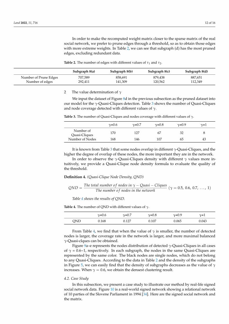
In order to make the recomputed weight matrix closer to the sparse matrix of the real social network, we prefer to prune edges through a threshold, so as to obtain those edges with more extreme weights. In Table 2, we can see that subgraph (d) has the most pruned edges, excluding redundant data.

(a) (b)

(c) (d)

Figure 8. The distribution of node degrees with different thresholds. The subgraph (a) is the distri-bution of node degree with thresholds Mean(AMP) and Mean(AMN); subgraph (b) is the distribu-tion of node degree with thresholds Mean(AMP) + Std(AMP) and Mean(AMN) − Std(AMN); subgraph (c) is the distribution of node degree with thresholds Mean(AMP) + 2 × Std(AMP) and Mean(AMN) − 2 × Std(AMN); subgraph (c) is the distribution of node degree with thresholds Mean(AMP) + 3 × Std(AMP) and Mean(AMN) – 3 × Std(AMN).

Table 2. The number of edges with different values of 𝜏1 and 𝜏2.

Subgraph 8(a) Subgraph 8(b) Subgraph 8(c) Subgraph 8(d) Number of Prune Edges 707,589 858,691 879,438 887,651

Number of edges 292,411 141,309 120,562 112,349

2 The value determination of 𝛾

Figure 8. The distribution of node degrees with different thresholds. The subgraph (a) is thedistribution of node degree with thresholds Mean(AMP) and Mean(AMN); subgraph (b) is the dis-tribution of node degree with thresholds Mean(AMP) + Std(AMP) and Mean(AMN) − Std(AMN);subgraph (c) is the distribution of node degree with thresholds Mean(AMP) + 2 × Std(AMP) andMean(AMN) − 2 × Std(AMN); subgraph (d) is the distribution of node degree with thresholdsMean(AMP) + 3 × Std(AMP) and Mean(AMN) − 3 × Std(AMN).

Table 1. Different values of τ1 and τ2.

Subgraph (a) Subgraph (b) Subgraph (c) Subgraph (d)

τ1Mean(AMP) Mean(AMP) + Std(AMP) Mean(AMP) + 2 × Std(AMP) Mean(AMP) + 3 × Std(AMP)11,377.463 66,294.718 119,731.322 173,936.850

τ2Mean(AMN) Mean(AMN) − Std(AMN) Mean(AMN) − 2 × Std(AMN) Mean(AMN) − 3 × Std(AMN)−1074.750 −18,230.686 −35,300.547 −52,414.579

In addition to comparing the node degree centrality of the four thresholds, we alsocompare the number of edge prunings under different thresholds.

Land 2022, 11, 716 12 of 16

In order to make the recomputed weight matrix closer to the sparse matrix of the realsocial network, we prefer to prune edges through a threshold, so as to obtain those edgeswith more extreme weights. In Table 2, we can see that subgraph (d) has the most prunededges, excluding redundant data.

Table 2. The number of edges with different values of τ1 and τ2.

Subgraph 8(a) Subgraph 8(b) Subgraph 8(c) Subgraph 8(d)

Number of Prune Edges 707,589 858,691 879,438 887,651Number of edges 292,411 141,309 120,562 112,349

2 The value determination of γ

We input the dataset of Figure 8d in the previous subsection as the pruned dataset intoour model for the γ-Quasi-Cliques detection. Table 3 shows the number of Quasi-Cliquesand node coverage detected with different values of γ.

Table 3. The number of Quasi-Cliques and nodes coverage with different values of γ.

γ=0.6 γ=0.7 γ=0.8 γ=0.9 γ=1

Number ofQuasi-Cliques 170 127 67 32 8

Number of Nodes 168 146 107 65 43

It is known from Table 3 that some nodes overlap in different γ-Quasi-Cliques, and thehigher the degree of overlap of these nodes, the more important they are in the network.

In order to observe the γ-Quasi-Cliques density with different γ values more in-tuitively, we provide a Quasi-Clique node density formula to evaluate the quality ofthe threshold.

Definition 4. (Quasi-Clique Node Density, QND)

QND =The total number o f nodes in γ−Quasi− Cliques

The number o f nodes in the network(γ = 0.5, 0.6, 0.7, . . . , 1)

Table 4 shows the results of QND.

Table 4. The number of QND with different values of γ.

γ=0.6 γ=0.7 γ=0.8 γ=0.9 γ=1

QND 0.168 0.127 0.107 0.065 0.043

From Table 4, we find that when the value of γ is smaller, the number of detectednodes is larger, the coverage rate in the network is larger, and more maximal balancedγ-Quasi-clques can be obtained.

Figure 9a–e represents the nodes distribution of detected γ-Quasi-Cliques in all casesof γ = 0.6~1, respectively. In each subgraph, the nodes in the same Quasi-Cliques arerepresented by the same color. The black nodes are single nodes, which do not belongto any Quasi-Cliques. According to the data in Table 2 and the density of the subgraphsin Figure 5, we can easily find that the density of subgraphs decreases as the value of γincreases. When γ = 0.6, we obtain the densest clustering result.

4.2. Case Study

In this subsection, we present a case study to illustrate our method by real-life signedsocial network data. Figure 10 is a real-world signed network showing a relational networkof 10 parties of the Slovene Parliament in 1994 [34]. Here are the signed social network andthe matrix.

Land 2022, 11, 716 13 of 16

Land 2022, 11, x FOR PEER REVIEW 12 of 16

We input the dataset of Figure 8d in the previous subsection as the pruned dataset into our model for the 𝛾-Quasi-Cliques detection. Table 3 shows the number of Quasi-Cliques and node coverage detected with different values of 𝛾.

Table 3. The number of Quasi-Cliques and nodes coverage with different values of 𝛾.

𝜸 = 𝟎. 𝟔 𝜸 = 𝟎. 𝟕 𝜸 = 𝟎. 𝟖 𝜸 = 𝟎. 𝟗 𝜸 = 𝟏 Number of Quasi-

Cliques 170 127 67 32 8 Number of Nodes 168 146 107 65 43

It is known from Table 3 that some nodes overlap in different 𝛾-Quasi-Cliques, and the higher the degree of overlap of these nodes, the more important they are in the net-work.

In order to observe the 𝛾-Quasi-Cliques density with different 𝛾 values more intui-tively, we provide a Quasi-Clique node density formula to evaluate the quality of the threshold.

Definition 4. (Quasi-Clique Node Density, QND) 𝑄𝑁𝐷 = (𝛾 = 0.5, 0.6, 0.7, … , 1)

Table 4 shows the results of QND.

Table 4. The number of QND with different values of 𝛾.

𝜸 = 𝟎. 𝟔 𝜸 = 𝟎. 𝟕 𝜸 = 𝟎. 𝟖 𝜸 = 𝟎. 𝟗 𝜸 = 𝟏 QND 0.168 0.127 0.107 0.065 0.043

From Table 4, we find that when the value of 𝛾 is smaller, the number of detected nodes is larger, the coverage rate in the network is larger, and more maximal balanced 𝛾-Quasi-clques can be obtained.

Figure 9a–e represents the nodes distribution of detected 𝛾-Quasi-Cliques in all cases of 𝛾 = 0.6~1, respectively. In each subgraph, the nodes in the same Quasi-Cliques are rep-resented by the same color. The black nodes are single nodes, which do not belong to any Quasi-Cliques. According to the data in Table 2 and the density of the subgraphs in Figure 5, we can easily find that the density of subgraphs decreases as the value of 𝛾 increases. When 𝛾 = 0.6, we obtain the densest clustering result.

(a) (b) (c)

(d) (e)

Figure 9. Nodes distribution of the γ-Quasi-Cliques with different γ. (a) is the distribution of γ-Quasi-Cliques when the γ = 0.6; (b) is the distribution of γ-Quasi-Cliques when the γ = 0.7; (c) is thedistribution of γ-Quasi-Cliques when the γ = 0.8; (d) is the distribution of γ-Quasi-Cliques when theγ = 0.9; (e) is the distribution of γ-Quasi-Cliques when the γ = 1.

Land 2022, 11, x FOR PEER REVIEW 13 of 16

Figure 9. Nodes distribution of the 𝛾-Quasi-Cliques with different 𝛾. (a) is the distribution of 𝛾-Quasi-Cliques when the 𝛾 = 0.6; (b) is the distribution of 𝛾-Quasi-Cliques when the 𝛾 = 0.7; (c) is the distribution of 𝛾-Quasi-Cliques when the 𝛾 = 0.8; (d) is the distribution of 𝛾-Quasi-Cliques when the 𝛾 = 0.9; (e) is the distribution of 𝛾-Quasi-Cliques when the 𝛾 = 1.

4.2. Case Study In this subsection, we present a case study to illustrate our method by real-life signed

social network data. Figure 10 is a real-world signed network showing a relational net-work of 10 parties of the Slovene Parliament in 1994 [34]. Here are the signed social net-work and the matrix.

Figure 10. Ten parties of the Slovene Parliament.

By completing the weight matrix and running it in our model, we obtain Quasi-Cliques of different sizes according to different 𝛾 values.

Figure 11 shows the sub-network corresponding to the matrix AMP that retains all positive edges (since a detailed example has been given in the previous section, here, only the positive sub-network is used as an example to illustrate).

Figure 11. Subgraph with positive edges.

When 𝛾 = 0.6, there are two 0.6-Quasi-Cliques in QC(AMP), which are: {1,3,6,8,9}, {2,4,5,7,10}. For the nodes set {1,3,6,8,9}, 𝛾(|𝑉| − 1) = 0.6 × (5 − 1) = 2.4, and the degree of all nodes is 4; they are larger than 2.4, and they are suitable to the condition 𝑑𝑒𝑔𝐺 (𝑉) ≥ 𝛾(|𝑉| − 1).

Similarly, we find one Quasi-Cliques in QC(AMN), which is: {1,3,6,8,9,2,4,5,7,10}. Meanwhile, there is one 0.6-Quasi-Cliques in QC(AMT): {1,3,6,8,9,2,4,5,7,10}. Thus, we can obtain the maximal balanced 0.6-Quasi-Cliques: {{1,3,6,8,9},{2,4,5,7,10}}.

Figure 12 shows the results. The same color of nodes is the same Quasi-Cliques.

Figure 10. Ten parties of the Slovene Parliament.

By completing the weight matrix and running it in our model, we obtain Quasi-Cliquesof different sizes according to different γ values.

Figure 11 shows the sub-network corresponding to the matrix AMP that retains allpositive edges (since a detailed example has been given in the previous section, here, onlythe positive sub-network is used as an example to illustrate).

Land 2022, 11, x FOR PEER REVIEW 13 of 16

Figure 9. Nodes distribution of the 𝛾-Quasi-Cliques with different 𝛾. (a) is the distribution of 𝛾-Quasi-Cliques when the 𝛾 = 0.6; (b) is the distribution of 𝛾-Quasi-Cliques when the 𝛾 = 0.7; (c) is the distribution of 𝛾-Quasi-Cliques when the 𝛾 = 0.8; (d) is the distribution of 𝛾-Quasi-Cliques when the 𝛾 = 0.9; (e) is the distribution of 𝛾-Quasi-Cliques when the 𝛾 = 1.

4.2. Case Study In this subsection, we present a case study to illustrate our method by real-life signed

social network data. Figure 10 is a real-world signed network showing a relational net-work of 10 parties of the Slovene Parliament in 1994 [34]. Here are the signed social net-work and the matrix.

Figure 10. Ten parties of the Slovene Parliament.

By completing the weight matrix and running it in our model, we obtain Quasi-Cliques of different sizes according to different 𝛾 values.

Figure 11 shows the sub-network corresponding to the matrix AMP that retains all positive edges (since a detailed example has been given in the previous section, here, only the positive sub-network is used as an example to illustrate).

Figure 11. Subgraph with positive edges.

When 𝛾 = 0.6, there are two 0.6-Quasi-Cliques in QC(AMP), which are: {1,3,6,8,9}, {2,4,5,7,10}. For the nodes set {1,3,6,8,9}, 𝛾(|𝑉| − 1) = 0.6 × (5 − 1) = 2.4, and the degree of all nodes is 4; they are larger than 2.4, and they are suitable to the condition 𝑑𝑒𝑔𝐺 (𝑉) ≥ 𝛾(|𝑉| − 1).

Similarly, we find one Quasi-Cliques in QC(AMN), which is: {1,3,6,8,9,2,4,5,7,10}. Meanwhile, there is one 0.6-Quasi-Cliques in QC(AMT): {1,3,6,8,9,2,4,5,7,10}. Thus, we can obtain the maximal balanced 0.6-Quasi-Cliques: {{1,3,6,8,9},{2,4,5,7,10}}.

Figure 12 shows the results. The same color of nodes is the same Quasi-Cliques.

Figure 11. Subgraph with positive edges.

Land 2022, 11, 716 14 of 16

When γ = 0.6, there are two 0.6-Quasi-Cliques in QC(AMP), which are: {1,3,6,8,9},{2,4,5,7,10}. For the nodes set {1,3,6,8,9}, γ(|V| − 1) = 0.6 × (5 − 1) = 2.4, and the degree ofall nodes is 4; they are larger than 2.4, and they are suitable to the condition degG (V) ≥γ(|V| − 1).

Similarly, we find one Quasi-Cliques in QC(AMN), which is: {1,3,6,8,9,2,4,5,7,10}.Meanwhile, there is one 0.6-Quasi-Cliques in QC(AMT): {1,3,6,8,9,2,4,5,7,10}. Thus, we canobtain the maximal balanced 0.6-Quasi-Cliques: {{1,3,6,8,9},{2,4,5,7,10}}.

Figure 12 shows the results. The same color of nodes is the same Quasi-Cliques.

Land 2022, 11, x FOR PEER REVIEW 14 of 16

Figure 12. Quasi-Cliques of the Slovene Parliament.

Since nodes in a social network correspond to individuals, “places that individuals like to visit” can be regarded as attributes of nodes. Through text mining and other tech-nologies, we are able to mine large social networks with place attributes from social net-works such as Twitter, Facebook, and Weibo. Therefore, in real life, different communities have different types of third places to gather, such as cafes, parks, or religious churches. In practical application, we can provide reasonable references for the layout and planning of public places according to the different places mapped to the detected community.

To facilitate understanding the idea of this paper, we simulate that the nodes in the dataset in this case frequently visit some “third places”. Node attributes are as follows in Table 5:

Table 5. Simulate attributes of nodes.

Node Frequently Visited Third Place 1 Coffee, Church 2 Bar, Coffee, Community Center 3 Church, Park, Coffee 4 Park, Bar, Coffee, Community Center 5 Community Center, Coffee 6 Park, Church 7 Bar, Community Center, Coffee 8 Church, Coffee, Bar 9 Mall, Church

10 Park, Community Center, Coffee

From the above analysis, the social network contains two communities: C1: {1,3,6,8,9} and C2: {2,4,5,7,10}. According to the different attributes of the nodes simulated in Table 5, it is not difficult to find that the nodes in C1 often visit churches, while the nodes in C2 prefer to visit cafes and community centers.

5. Conclusions Communities in social networks often gather in some urban public places. In order

to make reasonable suggestions for urban land division, it is a meaningful topic to study how to effectively detect communities in signed social networks. This paper focuses on mining the maximal balanced 𝛾-Quasi-Cliques in signed networks for detecting commu-nities. We proposed a model to solve the problems in three steps: First, we recomputed the weights of edges based on the mutual influence of common friends, and we defined

Figure 12. Quasi-Cliques of the Slovene Parliament.

Since nodes in a social network correspond to individuals, “places that individuals liketo visit” can be regarded as attributes of nodes. Through text mining and other technologies,we are able to mine large social networks with place attributes from social networks such asTwitter, Facebook, and Weibo. Therefore, in real life, different communities have differenttypes of third places to gather, such as cafes, parks, or religious churches. In practicalapplication, we can provide reasonable references for the layout and planning of publicplaces according to the different places mapped to the detected community.

To facilitate understanding the idea of this paper, we simulate that the nodes in thedataset in this case frequently visit some “third places”. Node attributes are as follows inTable 5:

Table 5. Simulate attributes of nodes.

Node Frequently Visited Third Place

1 Coffee, Church

2 Bar, Coffee, Community Center

3 Church, Park, Coffee

4 Park, Bar, Coffee, Community Center

5 Community Center, Coffee

6 Park, Church

7 Bar, Community Center, Coffee

8 Church, Coffee, Bar

9 Mall, Church

10 Park, Community Center, Coffee

From the above analysis, the social network contains two communities: C1: {1,3,6,8,9}and C2: {2,4,5,7,10}. According to the different attributes of the nodes simulated in Table 5,

Land 2022, 11, 716 15 of 16

it is not difficult to find that the nodes in C1 often visit churches, while the nodes in C2prefer to visit cafes and community centers.

5. Conclusions

Communities in social networks often gather in some urban public places. In order tomake reasonable suggestions for urban land division, it is a meaningful topic to study howto effectively detect communities in signed social networks. This paper focuses on miningthe maximal balanced γ-Quasi-Cliques in signed networks for detecting communities. Weproposed a model to solve the problems in three steps: First, we recomputed the weights ofedges based on the mutual influence of common friends, and we defined and determinedsome threshold ( mean± n ∗ std), (n = 0, 1, 2 and 3) for our pruning data process. Second,we proposed three new definitions of matrixes AMP, AMN and AMT to calculate the γ-Quasi-Cliques with positive, negative or unweighted edges by FCA method, respectively. Third,We filtered and detected the maximal balanced γ-Quasi-Cliques. In the experiment, weapplied the real-life data to our model, and compared results with different γ. Additionally,to help readers understand the proposed model on an intuitive level, we provided a casestudy. Experiments proved its effectiveness. In the future, we will consider improving theefficiency of our algorithm for the dynamic signed social network.

Author Contributions: Conceptualization, Y.Y. and D.-S.P.; methodology, Y.Y., and F.H.; validation,Y.Y., S.P., and H.L.; formal analysis, Y.Y.; writing—original draft preparation, Y.Y.; writing—reviewand editing, D.-S.P.; supervision, D.-S.P. funding acquisition, D.-S.P. All authors have read and agreedto the published version of the manuscript.

Funding: This research was funded by the National Research Foundation of Korea, grant numberNRF-2022R1A2C1005921, the BK21 FOUR (Fostering Outstanding Universities for Research), grantnumber 5199990914048, the Natural Science Basic Research Plan in Shaanxi Province of China (GrantNo. 2022JM-371), and the Fundamental Research Funds for the Central Universities (Grant No.GK202103080).

Data Availability Statement: The data presented in this study are openly available in SNAP athttps://snap.stanford.edu/data/soc-sign-bitcoin-alpha.html, accessed on 10 July 2009, referencenumber [32–34].

Conflicts of Interest: The authors declare no conflict of interest.

References1. Ramon, O.; Dennis, B. The third place. Qual. Sociol. 1982, 5, 265–284.2. Park, J.; State, B.; Bhole, M.; Bailey, M.C.; Ahn, Y.Y. People, Places, and Ties: Landscape of social places and their social network

structures. arXiv 2021, arXiv:2101.04737.3. HaoYang, L. Research on Key Technologies of Graph Mining; China Knowledge Network: Beijing, China, 2017.4. Jung Hee, W.; Ji Woo, P.; Ahn, J.G. Cancer Patient Specific Driver Gene Identification by Personalized Gene Network and

PageRank. KIPS Trans. Softw. Data Eng. 2021, 10, 547–554.5. Taejin, K.; Heechan, K.; Soowon, L. Automatic Tag Classification from Sound Data for Graph-Based Music Recommendation.

KIPS Trans. Softw. Data Eng. 2021, 10, 399–406.6. Yongbin, Q.; Cun-quan, Z. A new multimembership clustering method. J. Ind. Manag. Optim. 2007, 3, 619.7. Silviu, M.; Bogdan, C.; Talel, A. Building a Signed Network from Interactions in Wikipedia. In Proceedings of the First ACM

SIGMOD Workshop on Databases and Social Networks (DBSocial), Athens, Greece, 12 June 2011; pp. 19–24.8. Liu, M.M.; Hu, Q.C.; Guo, J.F.; Chen, J. Link prediction algorithm for signed social networks based on local and global tightness.

J. Inf. Processing Syst. 2021, 17, 213–226.9. Timo, H. Friends and enemies: A model of signed network formation. Theor. Econ. 2017, 12, 1057–1087.10. Cartwright, D.; Harary, F. Structural balance: A generalization of Heider’s theory. Psychol. Rev. 1956, 63, 277. [CrossRef]11. Harary, F. On local balance and N-balance in signed graphs. Mich. Math. J. 1955, 3, 37–41. [CrossRef]12. Yang, Y.; Park, D.S.; Hao, F.; Peng, S.; Hong, M.P.; Lee, H. Detection of Maximal Balanced Clique in Signed Networks Based

on Improved Three-Way Concept Lattice and Modified Formal Concept Analysis. 2021. Available online: https://assets.researchsquare.com/files/rs-277245/v1_covered.pdf?c=1631863443 (accessed on 26 April 2021).

13. Yang, Y.; Hao, F.; Park, D.S.; Peng, S.; Lee, H.; Mao, M. Modelling Prevention and Control Strategies for COVID-19 Propagationwith Patient Contact Networks. Hum.-Cent. Comput. Inf. Sci. 2021, 11, 45.

Land 2022, 11, 716 16 of 16

14. Guimei, L.; Limsoon, W. Effective Pruning Techniques for Mining Quasi-Cliques. In Proceedings of the Joint European Con-ference on Machine Learning and Knowledge Discovery in Databases, Antwerp, Belgium, 15–19 September 2008; Springer:Berlin/Heidelberg, Germany, 2008; pp. 33–49.

15. Fei, H.; Zheng, P.; Laurence, T.Y. Diversified top-k maximal clique detection in Social Internet of Things. Future Gener. Comput.Syst. 2020, 107, 408–417.

16. Doreian, P.; Mrvar, A. A partitioning approach to structural balance. Soc. Netw. 1996, 18, 149–168. [CrossRef]17. Yang, B.; Cheung, W.; Liu, J. Community mining from signed social networks. IEEE Trans. Knowl. Data Eng. 2007, 19, 1333–1348.

[CrossRef]18. Bansal, N.; Blum, A.; Chawla, S. Correlation clustering. Mach. Learn. 2004, 56, 89–113. [CrossRef]19. Sun, R.; Chen, C.; Wang, X.; Zhang, Y.; Wang, X. Stable Community Detection in Signed Social Networks. IEEE Trans. Knowl. Data

Eng. 2020. [CrossRef]20. Xia, C.; Luo, Y.; Wang, L.; Li, H.-J. A Fast Community Detection Algorithm Based on Reconstructing Signed Networks. IEEE Syst.

J. 2022, 16, 614–625. [CrossRef]21. Cadena, J.; Vullikanti, A.K.; Aggarwal, C.C. On dense subgraphs in signed network streams. In Proceedings of the 2016 IEEE 16th

International Conference on Data Mining (ICDM), Barcelona, Spain, 12–15 December 2016; pp. 51–60.22. Li, D.; Liu, J. Modeling influence diffusion over signed social networks. IEEE Trans. Knowl. Data Eng. 2019, 33, 613–625. [CrossRef]23. Tsourakakis, C.E.; Chen, T.; Kakimura, N.; Pachocki, J. Novel Dense Subgraph Discovery Primitives: Risk Aversion and Exclusion

Queries. In Proceedings of the Joint European Conference on Machine Learning and Knowledge Discovery in Databases,Würzburg, Germany, 6–20 September 2019; Springer: Cham, Switzerland, 2019; pp. 378–394.

24. Ordozgoiti, B.; Matakos, A.; Gionis, A. Finding large balanced subgraphs in signed networks. In Proceedings of the WebConference 2020, Taipei, Taiwan, 20–24 April 2020; pp. 1378–1388.

25. Qi, X.; Luo, R.; Fuller, E.; Luo, R.; Zhang, C.Q. Signed Quasi-Cliques merger: A new clustering method for signed networks withpositive and negative edges. Int. J. Pattern Recognit. Artif. Intell. 2016, 30, 1650006. [CrossRef]

26. Kleinfeld, J. Could it be a big world after all? The six degrees of separation myth. Society 2002, 12, 2–5.27. Hao, F.; Min, G.; Pei, Z.; Park, D.S.; Yang, L.T. K-clique community detection in social networks based on formal concept analysis.

IEEE Syst. J. 2015, 11, 250–259. [CrossRef]28. Yang, Y.; Hao, F.; Pang, B.; Min, G.; Wu, Y. Dynamic maximal cliques detection and evolution management in social internet of

things: A formal concept analysis approach. IEEE Trans. Netw. Sci. Eng. 2021. [CrossRef]29. Jo, Y.Y.; Kim, S.W.; Bae, D.H. Efficient sparse matrix multiplication on gpu for large social network analysis. In Proceedings of the

24th ACM International on Conference on Information and Knowledge Management, Melbourne, Australia, 18–23 October 2015;pp. 1261–1270.

30. Okasaki, C. From fast exponentiation to square matrices: An adventure in types. ACM SIGPLAN Not. 1999, 34, 28–35. [CrossRef]31. Zhang, J.; Zhou, X. A parallel algorithm for matrix fast exponentiation based on MPI. In Proceedings of the 2018 IEEE 3rd

International Conference on Big Data Analysis (ICBDA), Shanghai, China, 9–12 March 2018; pp. 162–165.32. Kumar, S.; Spezzano, F.; Subrahmanian, V.S.; Faloutsos, C. Edge Weight Prediction in Weighted Signed Networks. In Proceedings

of the 2016 IEEE 16th International Conference on Data Mining (ICDM), Barcelona, Spain, 12–15 December 2016.33. Kumar, S.; Hooi, B.; Makhija, D.; Kumar, M.; Subrahmanian, V.S.; Faloutsos, C. REV2: Fraudulent User Prediction in Rating

Platforms. In Proceedings of the 11th ACM International Conference on Web Searchand Data Mining (WSDM), Los Angeles, CA,USA, 5–9 February 2018.

34. Ferligoj, A.; Kramberger, A. An analysis of the slovene parliamentary parties network. Dev. Stat. Methodol. 1996, 12, 209–216.