SIViP (2009) 3:157–170DOI 10.1007/s11760-008-0067-2

ORIGINAL PAPER

A novel clipping technique for filtering FM signals embeddedin intensive noise

Alexey A. Roenko · Vladimir V. Lukin ·Igor Djurovic · Xu Zhengguang

Received: 21 August 2007 / Revised: 4 June 2008 / Accepted: 5 June 2008 / Published online: 28 June 2008© Springer-Verlag London Limited 2008

Abstract A novel adaptive clipping technique for filter-ing a constant amplitude frequency modulated (FM) signalembedded in non-Gaussian noise is proposed. It is based onthe analysis and processing of the estimate of probabilitydensity function of a FM signal realization. As a result, mod-ifications of two robust estimators of FM signal amplitudeare proposed. It is shown that these estimators can be usedfor Gaussian and non-Gaussian heavy-tail environments. Theproposed clipping technique can exploit one or anotherobtained robust estimate of the signal amplitude for adap-tive setting a threshold. Analysis of signal estimate accuracyfor different noise environments is carried out. Compara-tive analysis of the obtained methods and known approachesbased on scanning window nonlinear filtering and optimalrobust L-DFT form is performed. It is demonstrated that theusage of clipping-based technique leads to the considerableimprovement of the FM signal filtering efficiency in compar-ison to the aforementioned known approaches for differentnoise environments and a wide range of input SNR values.

A. A. Roenko · V. V. LukinDepartment of Transmitters, Receivers and Signal Processing,National Aerospace University, Chkalova Str. 17,61070 Kharkov, Ukrainee-mail: lukin@xai.kharkov.ua

I. Djurovic (B)Electrical Engineering Department, University of Montenegro,81000 Podgorica, Montenegroe-mail: igordj@cg.ac.yu

X. ZhengguangElectrical Information Department, Communication SoftwareResearch and Development Center, Huazhong Universityof Science and Technology, Luoyu Road, 1037,430074 Wuhan, Chinae-mail: xraymail2004@yeah.net

Keywords Clipping technique · FM signal amplitudeestimation · Probability density function · Non-Gaussiannoise environment

1 Introduction

It is a well-known fact that the performance of commu-nication, radar, navigation and other systems considerablydepends both on the type and characteristics of signals usedand noise statistical characteristics [1–4]. Because of this,frequency (FM) or phase (PM) modulated and manipulatedsignals have found wide application in systems mentionedearlier. The theory of FM and PM signal processing forGaussian noise environment and quite large input SNR �1was developed several decades ago [5].

Since then, considerable attention has been paid to theanalysis of more complicated and practical situations. In par-ticular, input SNR �1 is often not so large, it can be of order1 . . . 10 or even less. Besides, in many practical applicationsnoise cannot be considered Gaussian [4, 6]. It has been dem-onstrated that more heavy-tailed distributions like α-stableand other ones occur to be more adequate for simulatingproperties of real-life noise [4, 6–10]. Moreover, commonlyreliable a priori information on noise statistics is absent orrestricted. Then, the task to remove noise becomes moreimportant (in comparison to the case of input SNR �1 andGaussian noise) but more complex.

Assume that we have the following generalized knowl-edge about signal and noise characteristics. An additive noisehas a symmetric probability density function (pdf) withrespect to the location parameter (usually zero). Besides, thisnoise can possess heavy tails (coefficient of kurtosis in thiscase is usually � 0) [6]. At the same time, exact intensity(variance) and pdf of noise is unknown. Such assumptions

123

158 SIViP (2009) 3:157–170

and practical situations are typical for modern radar, com-munication and computer systems and networks [3, 8]. Con-cerning signal component, we suppose that within observa-tion interval it has a constant amplitude and, at least, tens orhundreds of oscillation periods.

There are various techniques for filtering such additivemixture of signal and noise. Among them one can mentiona scanning window nonlinear filtering (SWNF-method) [11]and robust DFT [12, 13] based approaches. However, along-side with observed positive effects, these methods possesssome peculiarities and drawbacks. The optimal or reason-able selection of the window aperture size is one of the mainproblems of the SWNF approach. As a result, it is necessaryto know the signal spectrum in advance for proper choice ofSWNF type and parameters.

In turn, robust DFT-methods [12] might have anotherdrawback. In the case of their application to processing thesignals of relatively large number of samples (several hun-dreds or more) a large amount of calculations and large com-putation time are required. For example, in the case of themethod based on the optimal L-DFT forms it is necessary tocompute spectrum estimate for all considered values of trim-ming parameter to obtain its optimal value [13]. Besides, thetechnique based on the robust forms of the DFT could intro-duce spectral distortions that can deteriorate accuracy [12].

Therefore, the design of new filtering methods able to getaround the shortcomings of aforementioned techniques inthe considered applications is a crucial task. It is necessarythat the methods under design should be robust in wide sense[14]. This means that these methods should be able to per-form well enough in cases of Gaussian and heavy-tail noisesas well as to operate appropriately for a wide range of inputSNRs under a limited a priori information concerning whatis a real pdf of noise and what is input SNR.

In this paper, we propose two novel noise suppressionmethods on the basis of clipping algorithm. Note that clip-ping effects observed in processing of FM signals embeddedin non-Gaussian noise and/or interference have been thor-oughly studied in papers of Middleton and Spaulding [4, 9,10]. In particular, they analyzed the influence of clipping onoutput signal statistics. However, a distinctive difference ofour technique lies on the fact that we deal with robust esti-mation of the FM signal amplitude that can be carried outdigitally and, then, with adaptive setting the correspondingthreshold. The main problem in our technique is to designan accurate and robust algorithm for the estimation of theamplitude of the FM signal. For this purpose, modificationsof two robust estimators are developed.

The first technique is based on the inter-quantile differ-ences (PEAK-estimator). This estimator is originallyproposed for blind estimation of noise variance in [15]. How-ever, the images are generally low-pass signals and we needto make several modifications of this technique for estimating

amplitudes of signals corrupted by intensive noise. For thispurpose, we have studied pdf of the modulated signal ampli-tude for various types of noise and we have analyzed inter-quantile differences for typical noise environments. Based onthis analysis, we adjusted correcting factor of the estimator.The second estimator is based on the median of absolute devi-ations of processed signal realization (MMAD-estimator).This is modification of the approach from [11]. Again weneed some adjustment of this technique to be able to per-form accurate estimation for FM signals. It is shown thatthe designed methods can be used for different noise envi-ronments (Gaussian and heavy-tailed noise). The results arecompared to the nonlinear filtering methods (SWNF androbust DFT). It is demonstrated that our methods exhibit bet-ter performance.

The paper is organized as follows. The analysis of a reali-zation of noisy FM signal is carried out in Sect. 2. The prob-lem of amplitude estimation that appears in the case of noisepresence is also highlighted in this section. The proposedmodifications of robust estimators are presented in Sect. 3.Simulation results with comparative analysis of the achievedaccuracy for the proposed amplitude estimators are given inSect. 4. The application of designed and known methods toFM signal filtering is considered in Sect. 5 with example thatdemonstrates the denoising efficiency of the PEAK-method.

2 Sample distribution analysis for FM signal noisyrealization

The FM and PM signals used in communication systems andvarious classes of radar systems (e.g., in radio altimeters,Doppler velocity measuring devices [2], etc.) can be writtenas [1]

s(t) = A sin[ψ(t)] (1)

where ψ(t) denotes the oscillation phase; A is the carrierwave amplitude. In the case of PM signal, ψ(t) = ω0t +ksM(t); for FM signal −ψ(t) = ω0t + k

∫ t0 sM(t ′)dt ′ + ϕ0,

whereϕ0 denotes arbitrary initial phase, sM(t) is the modulat-ing signal and ω0 denotes the carrier wave frequency. Belowwe assume that signal has several oscillations (at least five)within observation interval t ∈[0; TS].

A sampled realization of FM signal s(n�t) corrupted bynoise ν(n�t) can be represented in the following way [2]:

z(n�t) = s(n�t)+ ν(n�t) (2)

where �t = 1/FB is the sampling rate, FB denotes a sam-pling frequency, n ∈ [1; N ] is a sample index and N =TS/�tdenotes the number of samples in the observed interval.

Due to noise, the values of z(n�t) can be outside the inter-val [−A; A]. Suppose now that one a priori knows A or has

123

SIViP (2009) 3:157–170 159

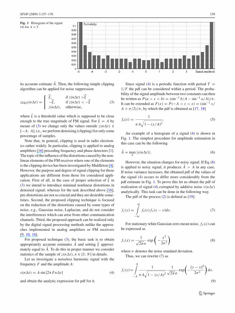
Fig. 1 Histogram of the signal(4) for A = 5

its accurate estimate A. Then, the following simple clippingalgorithm can be applied for noise suppression

zFILT(n�t) =⎧⎨

⎩

ξ , if z(n�t) >ξ−ξ , if z(n�t) < −ξz(n�t), otherwise,

(3)

where ξ is a threshold value which is supposed to be closeenough to the true magnitude of FM signal. For ξ = A bymeans of (3) we change only the values outside z(n�t) ∈[−A; A], i.e., we perform denoising (clipping) for only somepercentage of samples.

Note that, in general, clipping is used in radio electron-ics rather widely. In particular, clipping is applied to analogamplifiers [16] preceding frequency and phase detectors [1].The topic of the influence of the distortions caused by the non-linear elements of the FM receiver where one of the elementsis the clipping device has been investigated by Middleton [4].However, the purpose and degree of signal clipping for thoseapplications are different from those for considered appli-cation. First of all, in the case of proper selection of ξ in(3) we intend to introduce minimal nonlinear distortions indenoised signal; whereas for the task described above [16],pre-distortions are not so crucial and they are desirable some-times. Second, the proposed clipping technique is focusedon the reduction of the distortions caused by some types ofnoise, e.g., Gaussian noise, Laplacian, and do not considerthe interferences which can arise from other communicationchannels. Third, the proposed approach can be realized onlyby the digital signal processing methods unlike the approa-ches implemented in analog amplifiers or FM receivers[9, 10, 16].

For proposed technique (3), the basic task is to obtainappropriately accurate estimates A and setting ξ approxi-mately equal to A. To do this in proper manner we considerstatistics of the sample of z(n�t), n ∈ [1; N ] in details.

Let us investigate a noiseless harmonic signal with thefrequency F and the amplitude A:

s(n�t) = A sin [2πFn�t] (4)

and obtain the analytic expression for pdf for it.

Since signal (4) is a periodic function with period T =1/F the pdf can be considered within a period. The proba-bility of the signal amplitude between two constants can thenbe written as P(a < s < b) = (sin−1 b/A − sin−1 a/A)/π .It can be extended as F(x) = P(−A < s < x) = (sin−1 x/A + π/2)/π , by which the pdf is obtained as [17, 18]

fs(x) = 1

π A√

1 − (x/A)2. (5)

An example of a histogram of a signal (4) is shown inFig. 1. The simplest procedure for amplitude estimation inthis case can be the following

A = maxn

|s(n�t)|. (6)

However, the situation changes for noisy signal. If Eq. (6)is applied to noisy signal, it produces A > A in any case.If noise variance increases, the obtained pdf of the values ofthe signal (4) occurs to differ more considerably from thepdf estimate in Fig. 1. To prove this let us obtain the pdf ofrealization of signal (4) corrupted by additive noise ν(n�t)analytically. This task can be done in the following way.

The pdf of the process (2) is defined as [19]:

fz(y) =∞∫

−∞fs(x) fν(y − x)dx . (7)

For stationary white Gaussian zero-mean noise, fν(x) canbe expressed as

fν(x) = 1√2πσ

exp

(

− x2

2σ 2

)

(8)

where σ denotes the noise standard deviation.Thus, we can rewrite (7) as

fz(y)=A∫

−A

1

π A√

1 − (x/A)2

1√2πσ

exp

(

− [y − x]2

2σ 2

)

dx .

(9)

123

160 SIViP (2009) 3:157–170

Carrying the constant items out of the integral, expression(9) becomes

fz(y) = B1

A∫

−A

1√A2 − x2

exp

(

− [y − x]2

2σ 2

)

dx (10)

where B1 = 1πσ

√2π

.

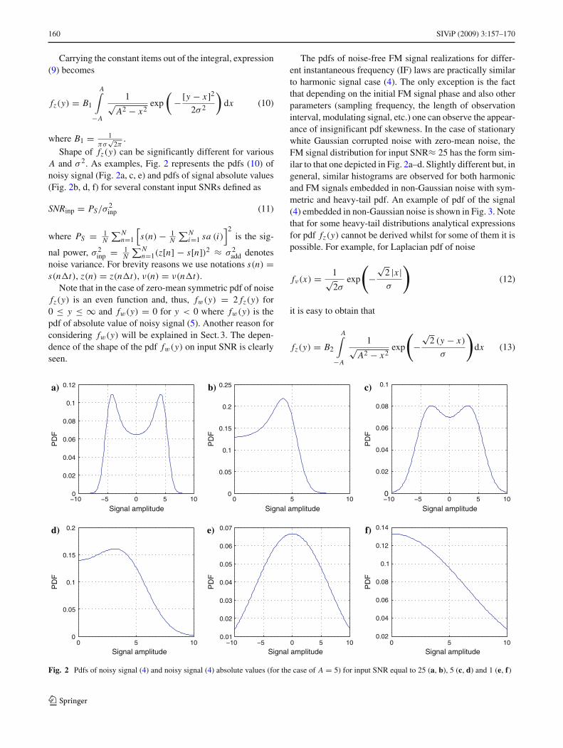
Shape of fz(y) can be significantly different for variousA and σ 2. As examples, Fig. 2 represents the pdfs (10) ofnoisy signal (Fig. 2a, c, e) and pdfs of signal absolute values(Fig. 2b, d, f) for several constant input SNRs defined as

SNRinp = PS/σ2inp (11)

where PS = 1N

∑Nn=1

[s(n)− 1

N

∑Ni=1 sa (i)

]2is the sig-

nal power, σ 2inp = 1

N

∑Nn=1(z[n] − s[n])2 ≈ σ 2

add denotesnoise variance. For brevity reasons we use notations s(n) =s(n�t), z(n) = z(n�t), ν(n) = ν(n�t).

Note that in the case of zero-mean symmetric pdf of noisefz(y) is an even function and, thus, fw(y) = 2 fz(y) for0 ≤ y ≤ ∞ and fw(y) = 0 for y < 0 where fw(y) is thepdf of absolute value of noisy signal (5). Another reason forconsidering fw(y) will be explained in Sect. 3. The depen-dence of the shape of the pdf fw(y) on input SNR is clearlyseen.

The pdfs of noise-free FM signal realizations for differ-ent instantaneous frequency (IF) laws are practically similarto harmonic signal case (4). The only exception is the factthat depending on the initial FM signal phase and also otherparameters (sampling frequency, the length of observationinterval, modulating signal, etc.) one can observe the appear-ance of insignificant pdf skewness. In the case of stationarywhite Gaussian corrupted noise with zero-mean noise, theFM signal distribution for input SNR≈ 25 has the form sim-ilar to that one depicted in Fig. 2a–d. Slightly different but, ingeneral, similar histograms are observed for both harmonicand FM signals embedded in non-Gaussian noise with sym-metric and heavy-tail pdf. An example of pdf of the signal(4) embedded in non-Gaussian noise is shown in Fig. 3. Notethat for some heavy-tail distributions analytical expressionsfor pdf fz(y) cannot be derived whilst for some of them it ispossible. For example, for Laplacian pdf of noise

fν(x) = 1√2σ

exp

(

−√

2 |x |σ

)

(12)

it is easy to obtain that

fz(y) = B2

A∫

−A

1√A2 − x2

exp

(

−√

2 (y − x)

σ

)

dx (13)

−10 −5 0 5 100

0.02

0.04

0.06

0.08

0.1

0.12

Signal amplitude

PD

F

0 5 100

0.05

0.1

0.15

0.2

0.25

Signal amplitude

PD

F

−10 −5 0 5 100

0.02

0.04

0.06

0.08

0.1

Signal amplitude

PD

F

0 5 100

0.05

0.1

0.15

0.2

Signal amplitude

PD

F

−10 −5 0 5 100.01

0.02

0.03

0.04

0.05

0.06

0.07

Signal amplitude

PD

F

0 5 100.02

0.04

0.06

0.08

0.1

0.12

0.14

Signal amplitude

PD

F

a) b) c)

d) e) f)

Fig. 2 Pdfs of noisy signal (4) and noisy signal (4) absolute values (for the case of A = 5) for input SNR equal to 25 (a, b), 5 (c, d) and 1 (e, f)

123

SIViP (2009) 3:157–170 161

where B2 = 1πσ

√2

. For the same input SNR, the shapes of

fz(y) in the case of Laplacian noise are similar to the shapesof fz(y) presented in Fig. 2.

Obviously, amplitude estimation by means of (6) for alimited size samples with distributions described by plots inFig. 2a–d will lead to incorrect results, i.e., the estimates Awill be greater than A especially if input SNR is small. More-over, the estimates A have the tendency to become larger ifnoise has heavier tail.

Therefore, it is necessary to apply other procedures forestimation of FM signal amplitude which would be robust toboth Gaussian noise and interferences with heavy-tail pdfs.Recall that these estimates have to perform well enough in awide range of possible input SNRs.

3 Proposed modifications of the robust amplitudeestimators

The first proposed way to obtaining an estimate A is based onshape analysis of pdf estimate for noisy input signal(Figs. 2a–e, 3a). Note that the largest number of sample val-ues is close to A and −A, i.e., the histogram has two mainpeaks (see Figs. 2a, c, 3a). This peculiarity can be exploitedfor an FM signal amplitude estimation by means of findinga coordinate of the maximum of processed signal realizationpdf estimate.

Below we propose modifications of the algorithms basedon inter-quantile differences [15] and median absolute devi-ation (MAD) [11] of processed signal realization. The directapplications of these algorithms to the estimation of the sig-nal amplitude produce biased estimates. To overcome thesedrawbacks correcting factors are exploited in the modifiedalgorithms. Their values are theoretically evaluated and prac-tically verified for different noise environments.

Now consider each algorithm for amplitude estimation indetails. There are several steps for calculating the amplitudeestimate based on inter-quantile difference. The first step is to

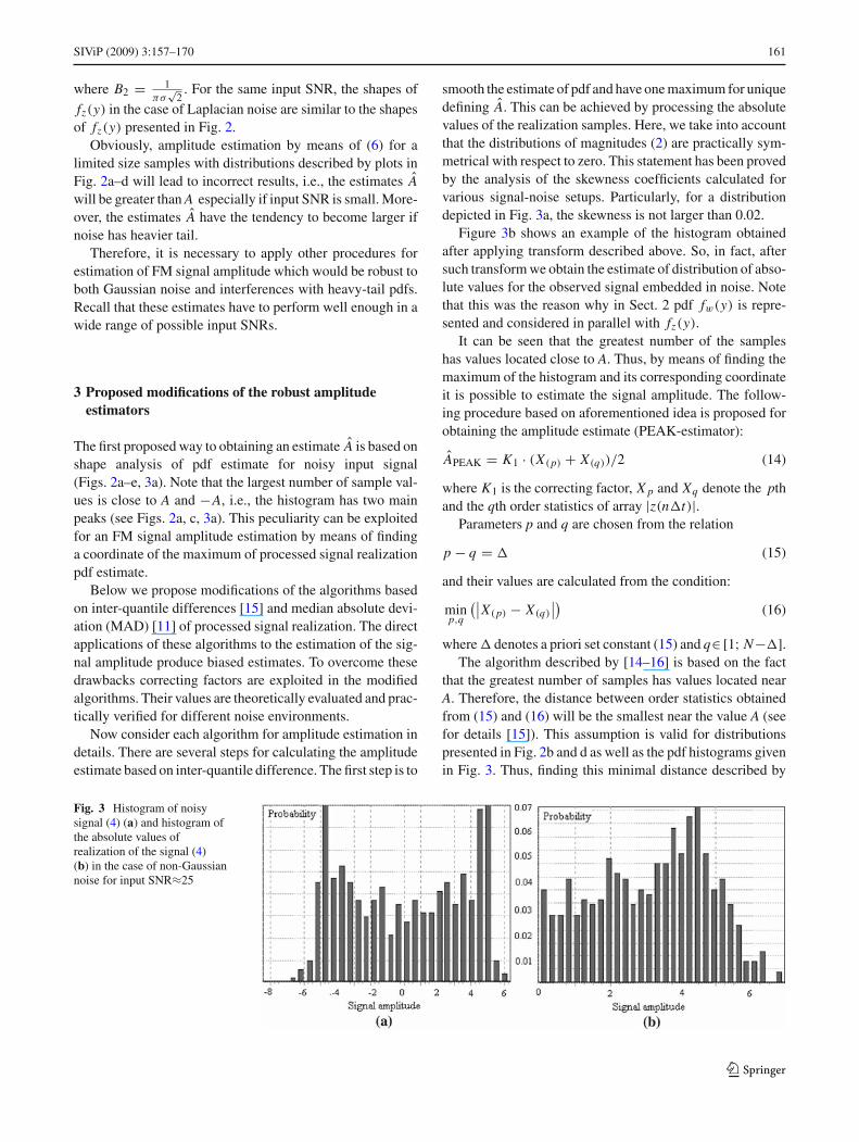
smooth the estimate of pdf and have one maximum for uniquedefining A. This can be achieved by processing the absolutevalues of the realization samples. Here, we take into accountthat the distributions of magnitudes (2) are practically sym-metrical with respect to zero. This statement has been provedby the analysis of the skewness coefficients calculated forvarious signal-noise setups. Particularly, for a distributiondepicted in Fig. 3a, the skewness is not larger than 0.02.

Figure 3b shows an example of the histogram obtainedafter applying transform described above. So, in fact, aftersuch transform we obtain the estimate of distribution of abso-lute values for the observed signal embedded in noise. Notethat this was the reason why in Sect. 2 pdf fw(y) is repre-sented and considered in parallel with fz(y).

It can be seen that the greatest number of the sampleshas values located close to A. Thus, by means of finding themaximum of the histogram and its corresponding coordinateit is possible to estimate the signal amplitude. The follow-ing procedure based on aforementioned idea is proposed forobtaining the amplitude estimate (PEAK-estimator):

APEAK = K1 · (X(p) + X(q))/2 (14)

where K1 is the correcting factor, X p and Xq denote the pthand the qth order statistics of array |z(n�t)|.

Parameters p and q are chosen from the relation

p − q = � (15)

and their values are calculated from the condition:

minp,q

(∣∣X(p) − X(q)∣∣) (16)

where� denotes a priori set constant (15) and q∈ [1; N−�].The algorithm described by [14–16] is based on the fact

that the greatest number of samples has values located nearA. Therefore, the distance between order statistics obtainedfrom (15) and (16) will be the smallest near the value A (seefor details [15]). This assumption is valid for distributionspresented in Fig. 2b and d as well as the pdf histograms givenin Fig. 3. Thus, finding this minimal distance described by

Fig. 3 Histogram of noisysignal (4) (a) and histogram ofthe absolute values ofrealization of the signal (4)(b) in the case of non-Gaussiannoise for input SNR≈25

123

162 SIViP (2009) 3:157–170

the values of p and q it is possible to obtain the amplitudeestimate by means of half-sum of the ordered statistics X(p)

and X(q).At the same time, for the distribution represented in Fig. 2f

the maximal concentration of sample values is observed forneighborhood of zero. Then it can be expected that the clip-ping technique based on PEAK-estimator would not performwell for small input SNRs.

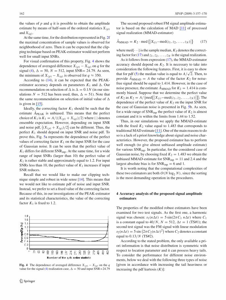
For visual confirmation of this property, Fig. 4 shows thedependence of averaged difference X(p) − X(q) on q for thesignal (4), � = 50, N = 512, input SNR= 24.79. As seen,the minimum of X(p) − X(q) is observed for q ≈ 350.

According to (14), it can be expected that the PEAK-estimator accuracy depends on parameters K1 and �. Ourrecommendation on selection of� is� = 0.1N (in our sim-ulations N = 512 has been used, thus, � = 51). Note thatthe same recommendation on selection of initial value of �is given in [15].

Ideally, the correcting factor K1 should be such that theestimate APEAK is unbiased. This means that the perfectchoice of K1 is K1 = A/〈(X(p) + X(q))/2〉where 〈·〉denotesensemble expectation. However, depending on input SNRand noise pdf,

⟨(X(p) + X(q))/2

⟩can be different. Thus, the

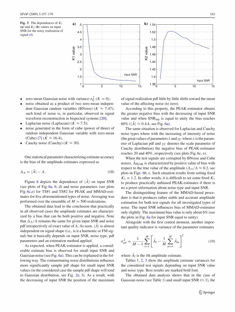
perfect K1 should depend on input SNR and noise pdf. Toprove this, Fig. 5a represents the dependence of the perfectvalues of correcting factor K1 on the input SNR for the caseof Gaussian noise. It can be seen that the perfect value ofK1 differs for different SNRinp. At the same time, for a widerange of input SNRs (larger than 10) the perfect value ofK1 is rather stable and approximately equal to 1.2. For inputSNRs less than 10, the perfect value of K1 increases if inputSNR reduces.

Recall that we would like to make our clipping tech-nique simple and robust in wide sense [14]. This means thatwe would not like to estimate pdf of noise and input SNR.Instead, we prefer to set a fixed value of the correcting factor.Because of this, in our investigations of the PEAK-estimatorand its statistical characteristics, the value of the correctingfactor K1 is fixed to 1.2.

Fig. 4 The dependence of averaged difference X(p) − X(q) on the qvalue for the signal (4) realization case,� = 50 and input SNR = 24.79

The second proposed robust FM signal amplitude estima-tor is based on the calculation of MAD [11] of processedsignal realization (MMAD-estimator)

AMMAD = K2 · med{∣∣X(i)−med(z1, z2, . . . , zN )

∣∣} (17)

where med{· · ·} is the sample median, K2 denotes the correct-ing factor for (17) and z1, z2, . . . , zN is the signal realization.

As it follows from expression (17), the MMAD-estimatoraccuracy should depend on K2. It is necessary to take intoconsideration the following features. First, it is easy to showthat for pdf (5) the median value is equal to A/

√2. Then, to

provide AMMAD = A the value of the factor K2 for noise-free signal should be equal to 1.414. However, in the case ofnoise presence, the estimate AMMAD for K2 = 1.414 is com-monly biased. Suppose that we determine the perfect valueof K2 as K2 = A/

⟨med

{∣∣X(i)−med(z1, z2, . . . , zN )∣∣}⟩. The

dependence of the perfect value of K2 on the input SNR forthe case of Gaussian noise is presented in Fig. 5b. As seen,for a wide range of SNRinp the perfect value of K2 is almostconstant and it is within the limits from 1.44 to 1.52.

Thus, in our simulations we apply the MMAD-estimatewith the fixed K2 value equal to 1.483 that corresponds totraditional MAD estimate [11]. One of the main reasons to doso is a lack of a priori knowledge about signal and noise char-acteristics. However, the proposed estimator has to performwell enough (to give almost unbiased amplitude estimate)for various SNRinp. In particular, for the considered case ofGaussian noise, by choosing fixed K2 = 1.483 we obtain theunbiased MMAD-estimate for SNRinp = 11 and 2.4 and thelargest absolute bias is for SNRinp = 6 and 1.

It is worth noting that the computational complexities ofthese two estimators are both O(N log2 N ), since the sortingis the most demanding operation in the procedures.

4 Accuracy analysis of the proposed signal amplitudeestimators

The properties of the modified robust estimators have beenexamined for two test signals. As the first one, a harmonicsignal was chosen: s1(n�t) = 5 sin(2πC1 n�t) where C1

is a constant equal to 40/N , N = 512, �t = 1 (TS#1); thesecond test signal was the FM signal with linear modulations2(n�t) = 5 sin

(2πC2(n�t)2

)where C2 denotes a constant

equal to 0.13/N (TS#2).According to the stated problem, the only available a pri-

ori information is that noise distribution is symmetric withrespect to location parameter and it can possess heavy tails.To consider the performance for different noise environ-ments, below we deal with the following three types of noise[given in accordance with increasing the tail heaviness orincreasing the pdf kurtosis (K)]:

123

SIViP (2009) 3:157–170 163

Fig. 5 The dependences of K1(a) and K2 (b) values on inputSNR for the noisy realization ofsignal (4)

0 5 10 151

1.5

2

2.5

3

3.5

4

4.5

5

Input SNRK

1 va

lue

0 5 10 151.38

1.4

1.42

1.44

1.46

1.48

1.5

1.52

1.54

Input SNR

K2

valu

e

a) b)

• zero-mean Gaussian noise with variance σ 2G (K = 0);

• noise obtained as a product of two zero-mean indepen-dent Gaussian random variables (BNoise) (K ≈ 7.47);such kind of noise is, in particular, observed in signalwaveform reconstruction in bispectral systems [20];

• Laplacian noise (Laplacian) (K ≈ 7.5);• noise generated in the form of cube (power of three) of

random independent Gaussian variable with zero-mean(Cube) [7] (K ≈ 16.4);

• Cauchy noise (Cauchy) (K ≈ 30).

One statistical parameter characterizing estimate accuracyis the bias of the amplitude estimates expressed as

�A = 〈 A〉 − A. (18)

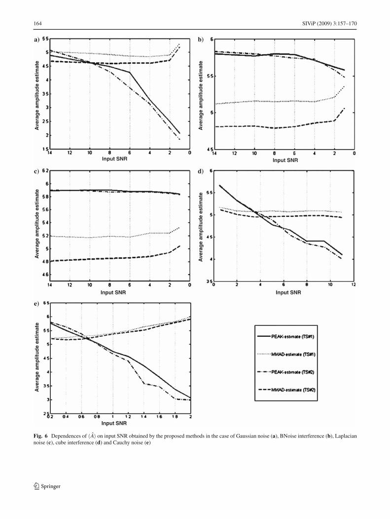
Figure 6 depicts the dependence of 〈 A〉 on input SNR(see plots of Fig. 6a, b, d) and noise parameters (see plotsFig. 6c,e) for TS#1 and TS#2 for PEAK and MMAD-esti-mates for five aforementioned types of noise. Averaging wasperformed over the ensemble of M = 500 realizations.

The obtained data lead to the conclusion that practicallyin all observed cases the amplitude estimates are character-ized by a bias that can be both positive and negative. Notethat �A/A remains the same for given input SNR and noisepdf irrespectively of exact value of A. As seen, 〈 A〉 is almostindependent on signal shape (i.e., is it a harmonic or FM sig-nal) but it basically depends on input SNR, noise type, pdfparameters and an estimation method applied.

As expected, when PEAK-estimator is applied, a consid-erable estimate bias is observed for small input SNR andGaussian noise (see Fig. 6a). This can be explained in the fol-lowing way. The contaminating noise distributions influencemore significantly sample pdf shape for small input SNRvalues (in the considered case the sample pdf shape will tendto Gaussian distribution, see Fig. 2e, f). As a result, withthe decreasing of input SNR the position of the maximum

of signal realization pdf little by little shifts toward the meanvalue of the affecting noise (to zero).

According to this property, the PEAK-estimator obtainsthe greater negative bias with the decreasing of input SNRvalue and when SNRinp is equal to unity the bias reaches60% (〈 A〉 ≈ 0.4A, see Fig. 6a).

The same situation is observed for Laplacian and Cauchynoise types where with the increasing of intensity of noise(the great values of parametersλ andγC whereλ is the param-eter of Laplacian pdf and γC denotes the scale parameter ofCauchy distribution) the negative bias of PEAK-estimatorreaches 20 and 40%, respectively (see plots Fig. 6c, e).

When the test signals are corrupted by BNoise and Cubenoises, APEAK is characterized by positive value of bias withrespect to the true value of the amplitude (�A/A ≈ 0.2, seeplots in Figs. 6b, c. Such situation results from setting fixedK1 = 1.2. In other words, it is difficult to set some fixed K1

to produce practically unbiased PEAK-estimates if there isno a priori information about noise type and input SNR.

The distinguishing feature of the MMAD-based proce-dure is that it produces rather stable and accurate amplitudeestimation for both test signals for all investigated types ofnoise. The input SNR influences bias of MMAD-estimatoronly slightly. The maximum bias value is only about 6% (seethe plots in Fig. 6a for input SNR equal to unity).

Alongside with the first central moment, another impor-tant quality indicator is variance of the parameter estimates

σ 2est = 1

M − 1

M∑

l=1

[

Al − 1

M

M∑

m=1

Am

]2

(19)

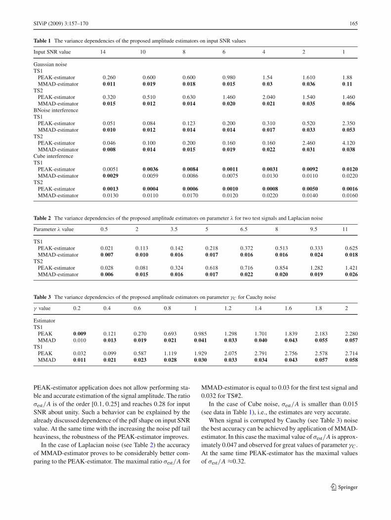
where Al is the lth amplitude estimate.Tables 1, 2, 3 show the amplitude estimate variances for

the considered test signals depending on input SNR valueand noise type. Best results are marked bold font.

The obtained data analysis shows that in the case ofGaussian noise (see Table 1) and small input SNR (≈ 1), the

123

164 SIViP (2009) 3:157–170

Fig. 6 Dependences of 〈 A〉 on input SNR obtained by the proposed methods in the case of Gaussian noise (a), BNoise interference (b), Laplaciannoise (c), cube interference (d) and Cauchy noise (e)

123

SIViP (2009) 3:157–170 165

Table 1 The variance dependencies of the proposed amplitude estimators on input SNR values

Input SNR value 14 10 8 6 4 2 1

Gaussian noiseTS1

PEAK-estimator 0.260 0.600 0.600 0.980 1.54 1.610 1.88MMAD-estimator 0.011 0.019 0.018 0.015 0.03 0.036 0.11

TS2PEAK-estimator 0.320 0.510 0.630 1.460 2.040 1.540 1.460MMAD-estimator 0.015 0.012 0.014 0.020 0.021 0.035 0.056

BNoise interferenceTS1

PEAK-estimator 0.051 0.084 0.123 0.200 0.310 0.520 2.350MMAD-estimator 0.010 0.012 0.014 0.014 0.017 0.033 0.053

TS2PEAK-estimator 0.046 0.100 0.200 0.160 0.160 2.460 4.120MMAD-estimator 0.008 0.014 0.015 0.019 0.022 0.031 0.038

Cube interferenceTS1

PEAK-estimator 0.0051 0.0036 0.0084 0.0011 0.0031 0.0092 0.0120MMAD-estimator 0.0029 0.0059 0.0086 0.0075 0.0130 0.0110 0.0220

TS2PEAK-estimator 0.0013 0.0004 0.0006 0.0010 0.0008 0.0050 0.0016MMAD-estimator 0.0130 0.0110 0.0170 0.0120 0.0220 0.0140 0.0160

Table 2 The variance dependencies of the proposed amplitude estimators on parameter λ for two test signals and Laplacian noise

Parameter λ value 0.5 2 3.5 5 6.5 8 9.5 11

TS1PEAK-estimator 0.021 0.113 0.142 0.218 0.372 0.513 0.333 0.625MMAD-estimator 0.007 0.010 0.016 0.017 0.016 0.016 0.024 0.018

TS2PEAK-estimator 0.028 0.081 0.324 0.618 0.716 0.854 1.282 1.421MMAD-estimator 0.006 0.015 0.016 0.017 0.022 0.020 0.019 0.026

Table 3 The variance dependencies of the proposed amplitude estimators on parameter γC for Cauchy noise

γ value 0.2 0.4 0.6 0.8 1 1.2 1.4 1.6 1.8 2

EstimatorTS1

PEAK 0.009 0.121 0.270 0.693 0.985 1.298 1.701 1.839 2.183 2.280MMAD 0.010 0.013 0.019 0.021 0.041 0.033 0.040 0.043 0.055 0.057

TS1PEAK 0.032 0.099 0.587 1.119 1.929 2.075 2.791 2.756 2.578 2.714MMAD 0.011 0.021 0.023 0.028 0.030 0.033 0.034 0.043 0.057 0.058

PEAK-estimator application does not allow performing sta-ble and accurate estimation of the signal amplitude. The ratioσest/A is of the order [0.1, 0.25] and reaches 0.28 for inputSNR about unity. Such a behavior can be explained by thealready discussed dependence of the pdf shape on input SNRvalue. At the same time with the increasing the noise pdf tailheaviness, the robustness of the PEAK-estimator improves.

In the case of Laplacian noise (see Table 2) the accuracyof MMAD-estimator proves to be considerably better com-paring to the PEAK-estimator. The maximal ratio σest/A for

MMAD-estimator is equal to 0.03 for the first test signal and0.032 for TS#2.

In the case of Cube noise, σest/A is smaller than 0.015(see data in Table 1), i.e., the estimates are very accurate.

When signal is corrupted by Cauchy (see Table 3) noisethe best accuracy can be achieved by application of MMAD-estimator. In this case the maximal value of σest/A is approx-imately 0.047 and observed for great values of parameter γC .

At the same time PEAK-estimator has the maximal valuesof σest/A ≈0.32.

123

166 SIViP (2009) 3:157–170

Summarizing these results, the PEAK-estimator accuracyconsiderably depends on noise pdf. For Gaussian noise itsaccuracy is poor whilst for some types of heavy-tail pdf ofnoise (for example, Cube noise) the accuracy can be excel-lent. Such properties in the case of absence of a priori knowl-edge of noise pdf can be considered as a drawback of thePEAK-estimator.

In turn, for MMAD-estimator a weak dependence ofσest/A on the type of noise and input SNR takes place. σest/Ais commonly of the order [0.02, 0.03] reaching 0.07 in theworst case of intensive Gaussian noise (see Table 1).

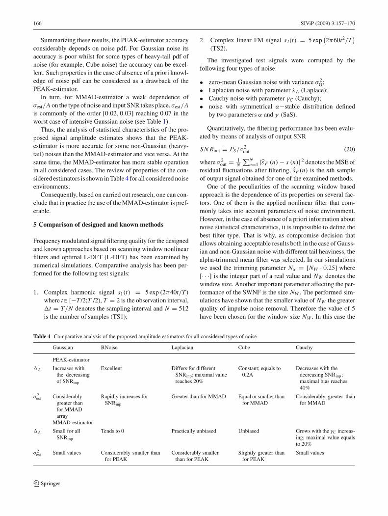
Thus, the analysis of statistical characteristics of the pro-posed signal amplitude estimates shows that the PEAK-estimator is more accurate for some non-Gaussian (heavy-tail) noises than the MMAD-estimator and vice versa. At thesame time, the MMAD-estimator has more stable operationin all considered cases. The review of properties of the con-sidered estimators is shown in Table 4 for all considered noiseenvironments.

Consequently, based on carried out research, one can con-clude that in practice the use of the MMAD-estimator is pref-erable.

5 Comparison of designed and known methods

Frequency modulated signal filtering quality for the designedand known approaches based on scanning window nonlinearfilters and optimal L-DFT (L-DFT) has been examined bynumerical simulations. Comparative analysis has been per-formed for the following test signals:

1. Complex harmonic signal s1(t) = 5 exp (2π40t/T)where t∈ [−T /2;T /2), T = 2 is the observation interval,�t = T/N denotes the sampling interval and N = 512is the number of samples (TS1);

2. Complex linear FM signal s2(t) = 5 exp(2π60t2/T

)

(TS2).

The investigated test signals were corrupted by thefollowing four types of noise:

• zero-mean Gaussian noise with variance σ 2G;

• Laplacian noise with parameter λL (Laplace);• Cauchy noise with parameter γC (Cauchy);• noise with symmetrical α−stable distribution defined

by two parameters α and γ (SaS).

Quantitatively, the filtering performance has been evalu-ated by means of analysis of output SNR

SN Rout = PS/σ2out (20)

where σ 2out = 1

N

∑Nn=1 |s F (n)− s (n)| 2 denotes the MSE of

residual fluctuations after filtering, sF (n) is the nth sampleof output signal obtained for one of the examined methods.

One of the peculiarities of the scanning window basedapproach is the dependence of its properties on several fac-tors. One of them is the applied nonlinear filter that com-monly takes into account parameters of noise environment.However, in the case of absence of a priori information aboutnoise statistical characteristics, it is impossible to define thebest filter type. That is why, as compromise decision thatallows obtaining acceptable results both in the case of Gauss-ian and non-Gaussian noise with different tail heaviness, thealpha-trimmed mean filter was selected. In our simulationswe used the trimming parameter Nα = [NW · 0.25] where[· · ·] is the integer part of a real value and NW denotes thewindow size. Another important parameter affecting the per-formance of the SWNF is the size NW . The performed sim-ulations have shown that the smaller value of NW the greaterquality of impulse noise removal. Therefore the value of 5have been chosen for the window size NW . In this case the

Table 4 Comparative analysis of the proposed amplitude estimators for all considered types of noise

Gaussian BNoise Laplacian Cube Cauchy

PEAK-estimator

�A Increases withthe decreasingof SNRinp

Excellent Differs for differentSNRinp; maximal valuereaches 20%

Constant; equals to0.2A

Decreases with thedecreasing SNRinp;maximal bias reaches40%

σ 2est Considerably

greater thanfor MMADarray

Rapidly increases forSNRinp

Greater than for MMAD Equal or smaller thanfor MMAD

Considerably greater thanfor MMAD

MMAD-estimator

�A Small for allSNRinp

Tends to 0 Practically unbiased Unbiased Grows with the γC increas-ing; maximal value equalsto 20%

σ 2est Small values Considerably smaller than

for PEAKConsiderably smaller

than for PEAKSlightly greater than

for PEAKSmall values

123

SIViP (2009) 3:157–170 167

number of trimmed samples has been 2 (one maximal andone minimal values, respectively).

In robust DFT based processing approach different formsof DFT can be obtained depending on the applied estimators.One of them is the robust DFT form which is based on therobust estimators from the L-class. L-DFT method describedin [13] uses the alpha-trimmed mean estimator with adop-tively selected value of trimming parameter for each con-sidered case. Thus, in situations when a priori knowledgeabout noise statistical characteristics partially or fully unde-fined such an L-DFT method can allow to obtain spectrumestimate close to the optimal. That is the efficiency of noisesuppression can be very high.

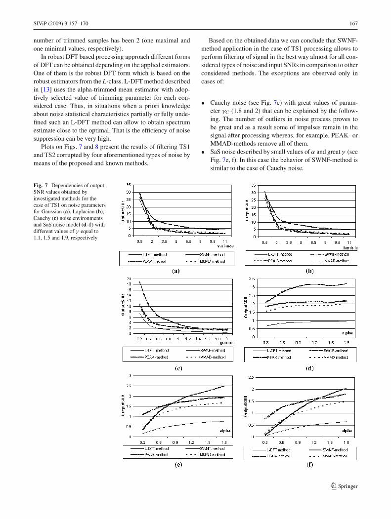
Plots on Figs. 7 and 8 present the results of filtering TS1and TS2 corrupted by four aforementioned types of noise bymeans of the proposed and known methods.

Based on the obtained data we can conclude that SWNF-method application in the case of TS1 processing allows toperform filtering of signal in the best way almost for all con-sidered types of noise and input SNRs in comparison to otherconsidered methods. The exceptions are observed only incases of:

• Cauchy noise (see Fig. 7c) with great values of param-eter γC (1.8 and 2) that can be explained by the follow-ing. The number of outliers in noise process proves tobe great and as a result some of impulses remain in thesignal after processing whereas, for example, PEAK- orMMAD-methods remove all of them.

• SaS noise described by small values of α and great γ (seeFig. 7e, f). In this case the behavior of SWNF-method issimilar to the case of Cauchy noise.

Fig. 7 Dependencies of outputSNR values obtained byinvestigated methods for thecase of TS1 on noise parametersfor Gaussian (a), Laplacian (b),Cauchy (c) noise environmentsand SaS noise model (d–f) withdifferent values of γ equal to1.1, 1.5 and 1.9, respectively

123

168 SIViP (2009) 3:157–170

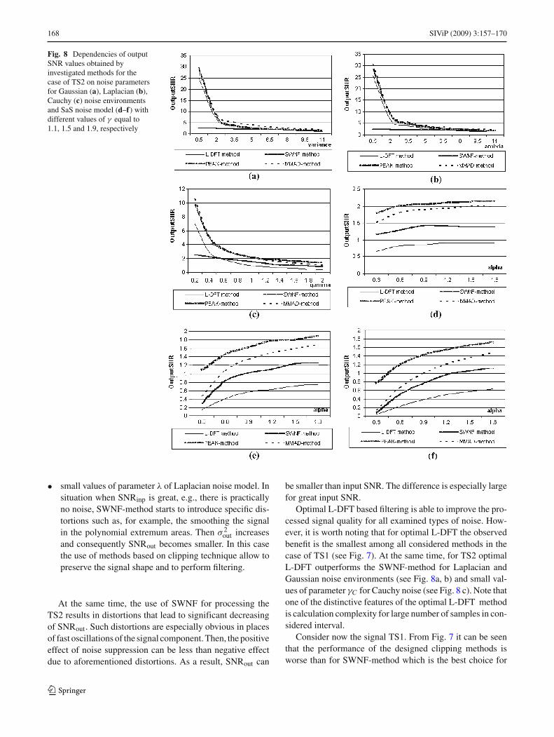
Fig. 8 Dependencies of outputSNR values obtained byinvestigated methods for thecase of TS2 on noise parametersfor Gaussian (a), Laplacian (b),Cauchy (c) noise environmentsand SaS noise model (d–f) withdifferent values of γ equal to1.1, 1.5 and 1.9, respectively

• small values of parameter λ of Laplacian noise model. Insituation when SNRinp is great, e.g., there is practicallyno noise, SWNF-method starts to introduce specific dis-tortions such as, for example, the smoothing the signalin the polynomial extremum areas. Then σ 2

out increasesand consequently SNRout becomes smaller. In this casethe use of methods based on clipping technique allow topreserve the signal shape and to perform filtering.

At the same time, the use of SWNF for processing theTS2 results in distortions that lead to significant decreasingof SNRout. Such distortions are especially obvious in placesof fast oscillations of the signal component. Then, the positiveeffect of noise suppression can be less than negative effectdue to aforementioned distortions. As a result, SNRout can

be smaller than input SNR. The difference is especially largefor great input SNR.

Optimal L-DFT based filtering is able to improve the pro-cessed signal quality for all examined types of noise. How-ever, it is worth noting that for optimal L-DFT the observedbenefit is the smallest among all considered methods in thecase of TS1 (see Fig. 7). At the same time, for TS2 optimalL-DFT outperforms the SWNF-method for Laplacian andGaussian noise environments (see Fig. 8a, b) and small val-ues of parameter γC for Cauchy noise (see Fig. 8 c). Note thatone of the distinctive features of the optimal L-DFT methodis calculation complexity for large number of samples in con-sidered interval.

Consider now the signal TS1. From Fig. 7 it can be seenthat the performance of the designed clipping methods isworse than for SWNF-method which is the best choice for

123

SIViP (2009) 3:157–170 169

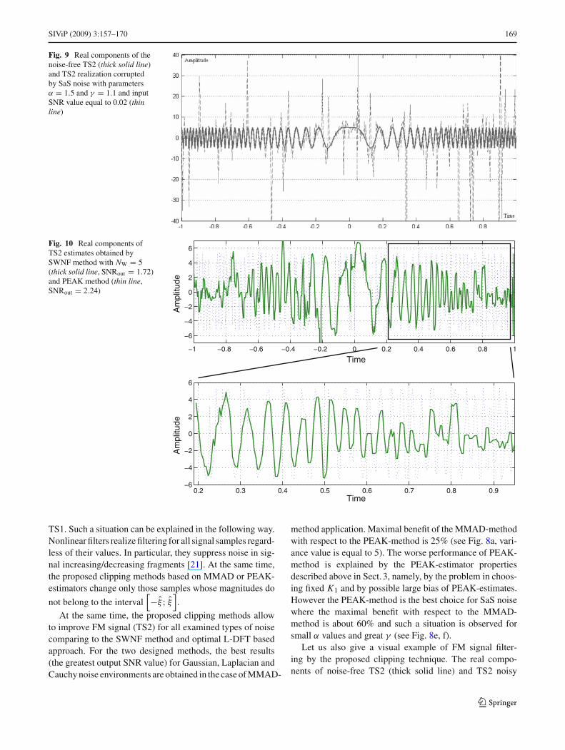
Fig. 9 Real components of thenoise-free TS2 (thick solid line)and TS2 realization corruptedby SaS noise with parametersα = 1.5 and γ = 1.1 and inputSNR value equal to 0.02 (thinline)

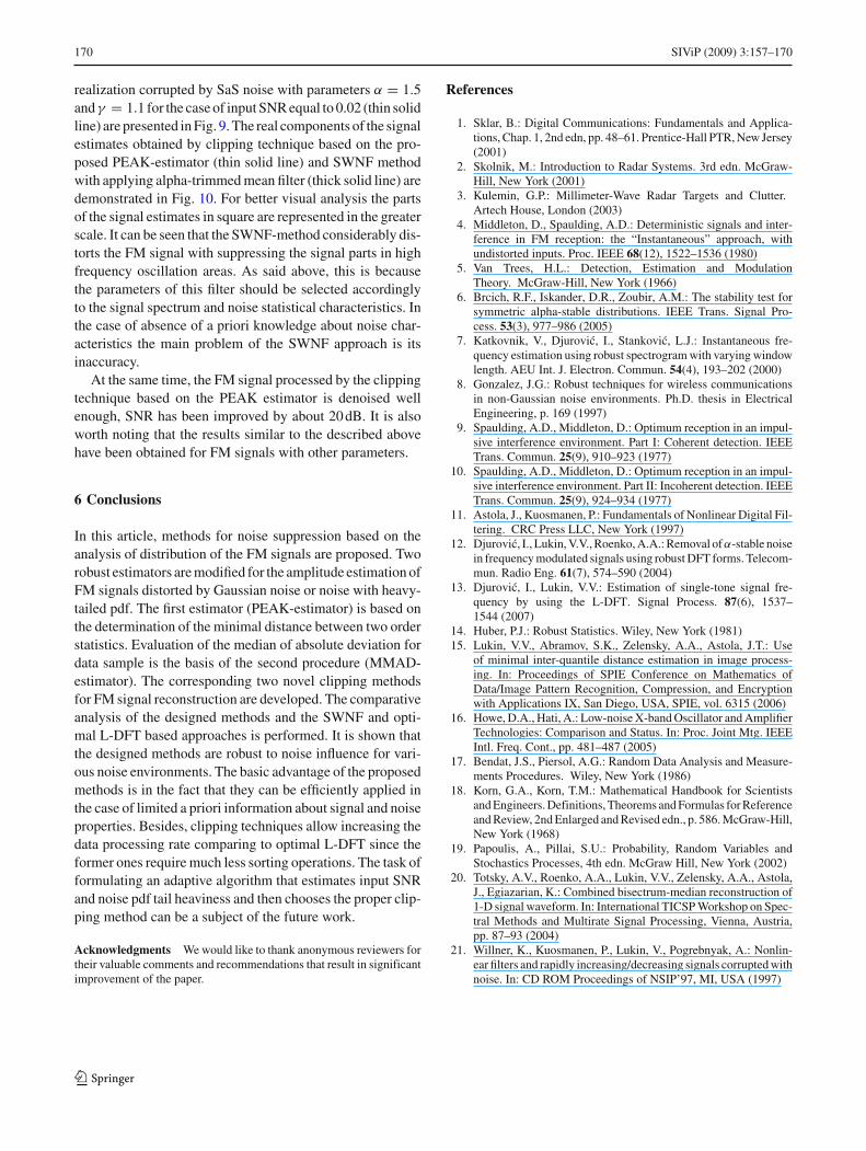
Fig. 10 Real components ofTS2 estimates obtained bySWNF method with NW = 5(thick solid line, SNRout = 1.72)and PEAK method (thin line,SNRout = 2.24)

−1 −0.8 −0.6 −0.4 −0.2 0 0.2 0.4 0.6 0.8 1

−6

−4

−2

0

2

4

6

Time

Am

plitu

de

0.2 0.3 0.4 0.5 0.6 0.7 0.8 0.9−6

−4

−2

0

2

4

6

Time

Am

plitu

de

TS1. Such a situation can be explained in the following way.Nonlinear filters realize filtering for all signal samples regard-less of their values. In particular, they suppress noise in sig-nal increasing/decreasing fragments [21]. At the same time,the proposed clipping methods based on MMAD or PEAK-estimators change only those samples whose magnitudes do

not belong to the interval[−ξ ; ξ

].

At the same time, the proposed clipping methods allowto improve FM signal (TS2) for all examined types of noisecomparing to the SWNF method and optimal L-DFT basedapproach. For the two designed methods, the best results(the greatest output SNR value) for Gaussian, Laplacian andCauchy noise environments are obtained in the case of MMAD-

method application. Maximal benefit of the MMAD-methodwith respect to the PEAK-method is 25% (see Fig. 8a, vari-ance value is equal to 5). The worse performance of PEAK-method is explained by the PEAK-estimator propertiesdescribed above in Sect. 3, namely, by the problem in choos-ing fixed K1 and by possible large bias of PEAK-estimates.However the PEAK-method is the best choice for SaS noisewhere the maximal benefit with respect to the MMAD-method is about 60% and such a situation is observed forsmall α values and great γ (see Fig. 8e, f).

Let us also give a visual example of FM signal filter-ing by the proposed clipping technique. The real compo-nents of noise-free TS2 (thick solid line) and TS2 noisy

123

170 SIViP (2009) 3:157–170

realization corrupted by SaS noise with parameters α = 1.5andγ = 1.1 for the case of input SNR equal to 0.02 (thin solidline) are presented in Fig. 9. The real components of the signalestimates obtained by clipping technique based on the pro-posed PEAK-estimator (thin solid line) and SWNF methodwith applying alpha-trimmed mean filter (thick solid line) aredemonstrated in Fig. 10. For better visual analysis the partsof the signal estimates in square are represented in the greaterscale. It can be seen that the SWNF-method considerably dis-torts the FM signal with suppressing the signal parts in highfrequency oscillation areas. As said above, this is becausethe parameters of this filter should be selected accordinglyto the signal spectrum and noise statistical characteristics. Inthe case of absence of a priori knowledge about noise char-acteristics the main problem of the SWNF approach is itsinaccuracy.

At the same time, the FM signal processed by the clippingtechnique based on the PEAK estimator is denoised wellenough, SNR has been improved by about 20 dB. It is alsoworth noting that the results similar to the described abovehave been obtained for FM signals with other parameters.

6 Conclusions

In this article, methods for noise suppression based on theanalysis of distribution of the FM signals are proposed. Tworobust estimators are modified for the amplitude estimation ofFM signals distorted by Gaussian noise or noise with heavy-tailed pdf. The first estimator (PEAK-estimator) is based onthe determination of the minimal distance between two orderstatistics. Evaluation of the median of absolute deviation fordata sample is the basis of the second procedure (MMAD-estimator). The corresponding two novel clipping methodsfor FM signal reconstruction are developed. The comparativeanalysis of the designed methods and the SWNF and opti-mal L-DFT based approaches is performed. It is shown thatthe designed methods are robust to noise influence for vari-ous noise environments. The basic advantage of the proposedmethods is in the fact that they can be efficiently applied inthe case of limited a priori information about signal and noiseproperties. Besides, clipping techniques allow increasing thedata processing rate comparing to optimal L-DFT since theformer ones require much less sorting operations. The task offormulating an adaptive algorithm that estimates input SNRand noise pdf tail heaviness and then chooses the proper clip-ping method can be a subject of the future work.

Acknowledgments We would like to thank anonymous reviewers fortheir valuable comments and recommendations that result in significantimprovement of the paper.

References

1. Sklar, B.: Digital Communications: Fundamentals and Applica-tions, Chap. 1, 2nd edn, pp. 48–61. Prentice-Hall PTR, New Jersey(2001)

2. Skolnik, M.: Introduction to Radar Systems. 3rd edn. McGraw-Hill, New York (2001)

3. Kulemin, G.P.: Millimeter-Wave Radar Targets and Clutter.Artech House, London (2003)

4. Middleton, D., Spaulding, A.D.: Deterministic signals and inter-ference in FM reception: the “Instantaneous” approach, withundistorted inputs. Proc. IEEE 68(12), 1522–1536 (1980)

5. Van Trees, H.L.: Detection, Estimation and ModulationTheory. McGraw-Hill, New York (1966)

6. Brcich, R.F., Iskander, D.R., Zoubir, A.M.: The stability test forsymmetric alpha-stable distributions. IEEE Trans. Signal Pro-cess. 53(3), 977–986 (2005)

7. Katkovnik, V., Djurovic, I., Stankovic, L.J.: Instantaneous fre-quency estimation using robust spectrogram with varying windowlength. AEU Int. J. Electron. Commun. 54(4), 193–202 (2000)

8. Gonzalez, J.G.: Robust techniques for wireless communicationsin non-Gaussian noise environments. Ph.D. thesis in ElectricalEngineering, p. 169 (1997)

9. Spaulding, A.D., Middleton, D.: Optimum reception in an impul-sive interference environment. Part I: Coherent detection. IEEETrans. Commun. 25(9), 910–923 (1977)

10. Spaulding, A.D., Middleton, D.: Optimum reception in an impul-sive interference environment. Part II: Incoherent detection. IEEETrans. Commun. 25(9), 924–934 (1977)

11. Astola, J., Kuosmanen, P.: Fundamentals of Nonlinear Digital Fil-tering. CRC Press LLC, New York (1997)

12. Djurovic, I., Lukin, V.V., Roenko, A.A.: Removal ofα-stable noisein frequency modulated signals using robust DFT forms. Telecom-mun. Radio Eng. 61(7), 574–590 (2004)

13. Djurovic, I., Lukin, V.V.: Estimation of single-tone signal fre-quency by using the L-DFT. Signal Process. 87(6), 1537–1544 (2007)

14. Huber, P.J.: Robust Statistics. Wiley, New York (1981)15. Lukin, V.V., Abramov, S.K., Zelensky, A.A., Astola, J.T.: Use

of minimal inter-quantile distance estimation in image process-ing. In: Proceedings of SPIE Conference on Mathematics ofData/Image Pattern Recognition, Compression, and Encryptionwith Applications IX, San Diego, USA, SPIE, vol. 6315 (2006)

16. Howe, D.A., Hati, A.: Low-noise X-band Oscillator and AmplifierTechnologies: Comparison and Status. In: Proc. Joint Mtg. IEEEIntl. Freq. Cont., pp. 481–487 (2005)

17. Bendat, J.S., Piersol, A.G.: Random Data Analysis and Measure-ments Procedures. Wiley, New York (1986)

18. Korn, G.A., Korn, T.M.: Mathematical Handbook for Scientistsand Engineers. Definitions, Theorems and Formulas for Referenceand Review, 2nd Enlarged and Revised edn., p. 586. McGraw-Hill,New York (1968)

19. Papoulis, A., Pillai, S.U.: Probability, Random Variables andStochastics Processes, 4th edn. McGraw Hill, New York (2002)

20. Totsky, A.V., Roenko, A.A., Lukin, V.V., Zelensky, A.A., Astola,J., Egiazarian, K.: Combined bisectrum-median reconstruction of1-D signal waveform. In: International TICSP Workshop on Spec-tral Methods and Multirate Signal Processing, Vienna, Austria,pp. 87–93 (2004)

21. Willner, K., Kuosmanen, P., Lukin, V., Pogrebnyak, A.: Nonlin-ear filters and rapidly increasing/decreasing signals corrupted withnoise. In: CD ROM Proceedings of NSIP’97, MI, USA (1997)

123