A Nonlinear Case of the 1-D Backward Heat Problem: Regularization and Error Estimate
15
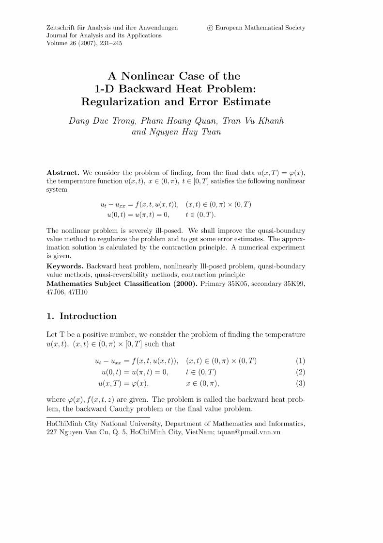
Zeitschrift f¨ ur Analysis und ihre Anwendungen c European Mathematical Society Journal for Analysis and its Applications Volume 26 (2007), 231–245 A Nonlinear Case of the 1-D Backward Heat Problem: Regularization and Error Estimate Dang Duc Trong, Pham Hoang Quan, Tran Vu Khanh and Nguyen Huy Tuan Abstract. We consider the problem of finding, from the final data u(x, T )= ϕ(x), the temperature function u(x, t),x ∈ (0,π),t ∈ [0,T ] satisfies the following nonlinear system u t - u xx = f (x, t, u(x, t)), (x, t) ∈ (0,π) × (0,T ) u(0,t)= u(π,t)=0, t ∈ (0,T ). The nonlinear problem is severely ill-posed. We shall improve the quasi-boundary value method to regularize the problem and to get some error estimates. The approx- imation solution is calculated by the contraction principle. A numerical experiment is given. Keywords. Backward heat problem, nonlinearly Ill-posed problem, quasi-boundary value methods, quasi-reversibility methods, contraction principle Mathematics Subject Classification (2000). Primary 35K05, secondary 35K99, 47J06, 47H10 1. Introduction Let T be a positive number, we consider the problem of finding the temperature u(x, t), (x, t) ∈ (0,π) × [0,T ] such that u t - u xx = f (x, t, u(x, t)), (x, t) ∈ (0,π) × (0,T ) (1) u(0,t)= u(π,t)=0, t ∈ (0,T ) (2) u(x, T )= ϕ(x), x ∈ (0,π), (3) where ϕ(x),f (x, t, z ) are given. The problem is called the backward heat prob- lem, the backward Cauchy problem or the final value problem. HoChiMinh City National University, Department of Mathematics and Informatics, 227 Nguyen Van Cu, Q. 5, HoChiMinh City, VietNam; [email protected]
-
Upload
independent -
Category
Documents
-
view
0 -
download
0
Transcript of A Nonlinear Case of the 1-D Backward Heat Problem: Regularization and Error Estimate
Zeitschrift fur Analysis und ihre Anwendungen c© European Mathematical SocietyJournal for Analysis and its ApplicationsVolume 26 (2007), 231–245
A Nonlinear Case of the1-D Backward Heat Problem:
Regularization and Error Estimate
Dang Duc Trong, Pham Hoang Quan, Tran Vu Khanhand Nguyen Huy Tuan
Abstract. We consider the problem of finding, from the final data u(x, T ) = ϕ(x),the temperature function u(x, t), x ∈ (0, π), t ∈ [0, T ] satisfies the following nonlinearsystem
ut − uxx = f(x, t, u(x, t)), (x, t) ∈ (0, π)× (0, T )
u(0, t) = u(π, t) = 0, t ∈ (0, T ).
The nonlinear problem is severely ill-posed. We shall improve the quasi-boundaryvalue method to regularize the problem and to get some error estimates. The approx-imation solution is calculated by the contraction principle. A numerical experimentis given.
Keywords. Backward heat problem, nonlinearly Ill-posed problem, quasi-boundaryvalue methods, quasi-reversibility methods, contraction principle
Mathematics Subject Classification (2000). Primary 35K05, secondary 35K99,47J06, 47H10
1. Introduction
Let T be a positive number, we consider the problem of finding the temperatureu(x, t), (x, t) ∈ (0, π)× [0, T ] such that
ut − uxx = f(x, t, u(x, t)), (x, t) ∈ (0, π)× (0, T ) (1)
u(0, t) = u(π, t) = 0, t ∈ (0, T ) (2)
u(x, T ) = ϕ(x), x ∈ (0, π), (3)
where ϕ(x), f(x, t, z) are given. The problem is called the backward heat prob-lem, the backward Cauchy problem or the final value problem.
HoChiMinh City National University, Department of Mathematics and Informatics,227 Nguyen Van Cu, Q. 5, HoChiMinh City, VietNam; [email protected]
232 D. D. Trong et al.
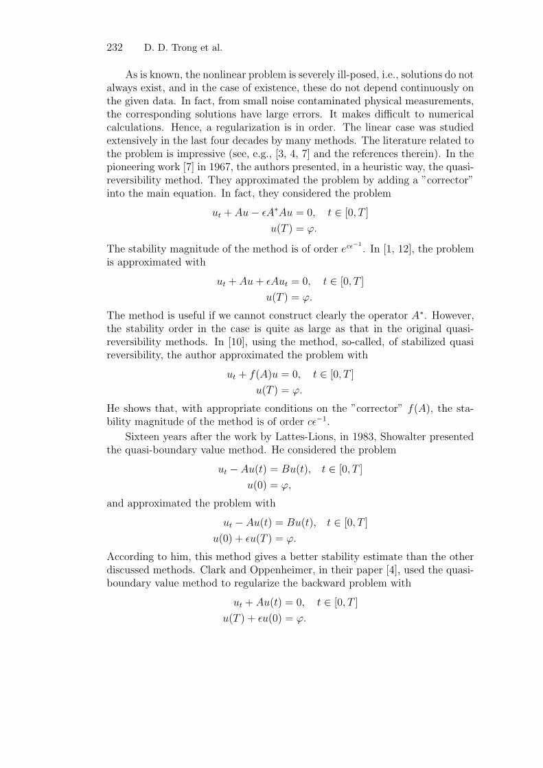
As is known, the nonlinear problem is severely ill-posed, i.e., solutions do notalways exist, and in the case of existence, these do not depend continuously onthe given data. In fact, from small noise contaminated physical measurements,the corresponding solutions have large errors. It makes difficult to numericalcalculations. Hence, a regularization is in order. The linear case was studiedextensively in the last four decades by many methods. The literature related tothe problem is impressive (see, e.g., [3, 4, 7] and the references therein). In thepioneering work [7] in 1967, the authors presented, in a heuristic way, the quasi-reversibility method. They approximated the problem by adding a ”corrector”into the main equation. In fact, they considered the problem
ut + Au− εA∗Au = 0, t ∈ [0, T ]u(T ) = ϕ.
The stability magnitude of the method is of order ecε−1
. In [1, 12], the problemis approximated with
ut + Au+ εAut = 0, t ∈ [0, T ]u(T ) = ϕ.
The method is useful if we cannot construct clearly the operator A∗. However,the stability order in the case is quite as large as that in the original quasi-reversibility methods. In [10], using the method, so-called, of stabilized quasireversibility, the author approximated the problem with
ut + f(A)u = 0, t ∈ [0, T ]u(T ) = ϕ.
He shows that, with appropriate conditions on the ”corrector” f(A), the sta-bility magnitude of the method is of order cε−1.
Sixteen years after the work by Lattes-Lions, in 1983, Showalter presentedthe quasi-boundary value method. He considered the problem
ut − Au(t) = Bu(t), t ∈ [0, T ]u(0) = ϕ,
and approximated the problem with
ut − Au(t) = Bu(t), t ∈ [0, T ]u(0) + εu(T ) = ϕ.
According to him, this method gives a better stability estimate than the otherdiscussed methods. Clark and Oppenheimer, in their paper [4], used the quasi-boundary value method to regularize the backward problem with
ut + Au(t) = 0, t ∈ [0, T ]u(T ) + εu(0) = ϕ.
1-D Backward Heat Problem 233
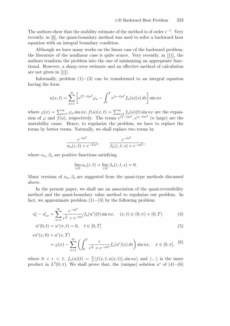
The authors show that the stability estimate of the method is of order ε−1. Veryrecently, in [6], the quasi-boundary method was used to solve a backward heatequation with an integral boundary condition.
Although we have many works on the linear case of the backward problem,the literature of the nonlinear case is quite scarce. Very recently, in [11], theauthors tranform the problem into the one of minimizing an appropriate func-tional. However, a sharp error estimate and an effective method of calculationare not given in [11].
Informally, problem (1)−(3) can be transformed to an integral equationhaving the form
u(x, t) =∞∑
n=1
[
e(T−t)n2
ϕn −∫ T
t
e(s−t)n2
fn(u)(s) ds
]
sinnx
where ϕ(x) =∑∞
n=1 ϕn sinnx, f(u)(x, t) =∑∞
n=1 fn(u)(t) sinnx are the expan-
sion of ϕ and f(u), respectively. The terms e(T−t)n2
, e(s−t)n2
(n large) are theunstability cause. Hence, to regularize the problem, we have to replace theterms by better terms. Naturally, we shall replace two terms by
e−tn2
αn(ε, t) + e−Tn2,
e−tn2
βn(ε, t, s) + e−sn2,
where αn, βn are positive functions satisfying
limε↓0
αn(ε, t) = limε↓0
βn(ε, t, s) = 0.
Many versions of αn, βn are suggested from the quasi-type methods discussedabove.
In the present paper, we shall use an association of the quasi-reversibilitymethod and the quasi-boundary value method to regularize our problem. Infact, we approximate problem (1)−(3) by the following problem:
uεt − uεxx =∞∑
n=1
e−tn2
εtT + e−tn2
fn(uε)(t) sinnx, (x, t) ∈ (0, π)× (0, T ) (4)
uε(0, t) = uε(π, t) = 0, t ∈ [0, T ] (5)
εuε(x, 0) + uε(x, T )
= ϕ(x)−∞∑
n=1
(∫ T
0
ε
εsT + e−sn2
fn(uε)(s) ds
)
sinnx, x ∈ [0, π], (6)
where 0 < ε < 1, fn(u)(t) =2π〈f(x, t, u(x, t)), sinnx〉 and 〈·, ·〉 is the inner
product in L2(0, π). We shall prove that, the (unique) solution uε of (4)−(6)
234 D. D. Trong et al.
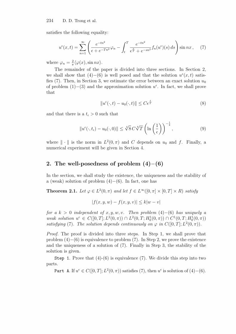
satisfies the following equality:
uε(x, t) =∞∑
n=1
(
e−tn2
ε+ e−Tn2ϕn −
∫ T
t
e−tn2
εsT + e−sn2
fn(uε)(s) ds
)
sinnx , (7)
where ϕn =2π〈ϕ(x), sinnx〉.
The remainder of the paper is divided into three sections. In Section 2,we shall show that (4)−(6) is well posed and that the solution uε(x, t) satis-fies (7). Then, in Section 3, we estimate the error between an exact solution u0
of problem (1)−(3) and the approximation solution uε. In fact, we shall provethat
‖uε(·, t)− u0(·, t)‖ ≤ CεtT (8)
and that there is a tε > 0 such that
‖uε(·, tε)− u0(·, 0)‖ ≤ 4√8C
4√T
(
ln
(
1
ε
))− 1
4
, (9)
where ‖ · ‖ is the norm in L2(0, π) and C depends on u0 and f . Finally, anumerical experiment will be given in Section 4.
2. The well-posedness of problem (4)−(6)
In the section, we shall study the existence, the uniqueness and the stability ofa (weak) solution of problem (4)−(6). In fact, one has
Theorem 2.1. Let ϕ ∈ L2(0, π) and let f ∈ L∞([0, π]× [0, T ]×R) satisfy
|f(x, y, w)− f(x, y, v)| ≤ k|w − v|
for a k > 0 independent of x, y, w, v. Then problem (4)−(6) has uniquely aweak solution uε ∈ C([0, T ];L2(0, π)) ∩ L2(0, T ;H1
0 (0, π)) ∩ C1(0, T ;H10 (0, π))
satisfying (7). The solution depends continuously on ϕ in C([0, T ];L2(0, π)).
Proof. The proof is divided into three steps. In Step 1, we shall prove thatproblem (4)−(6) is equivalence to problem (7). In Step 2, we prove the existenceand the uniqueness of a solution of (7). Finally in Step 3, the stability of thesolution is given.
Step 1. Prove that (4)-(6) is equivalence (7). We divide this step into twoparts.
Part A. If uε ∈ C([0, T ];L2(0, π)) satisfies (7), then uε is solution of (4)−(6).
1-D Backward Heat Problem 235
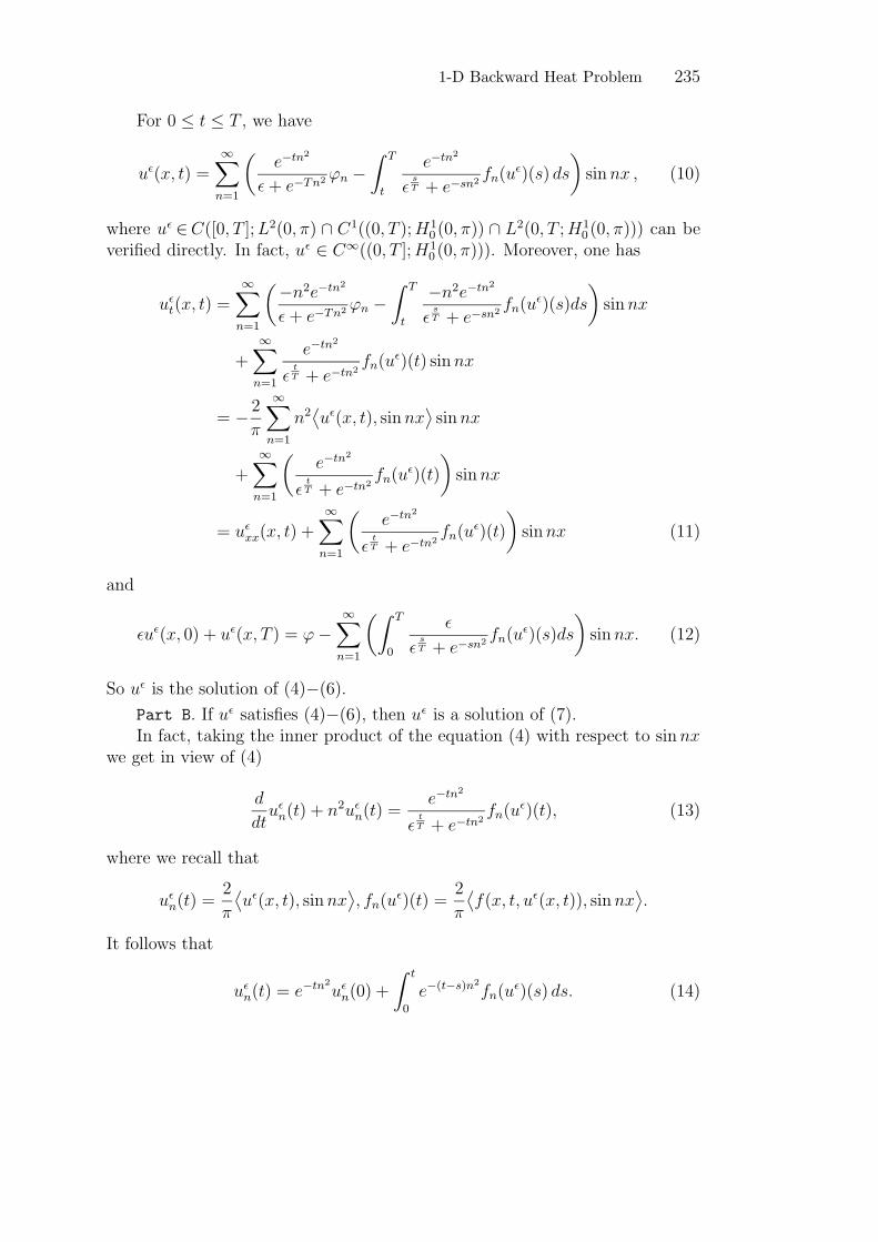
For 0 ≤ t ≤ T , we have
uε(x, t) =∞∑
n=1
(
e−tn2
ε+ e−Tn2ϕn −
∫ T
t
e−tn2
εsT + e−sn2
fn(uε)(s) ds
)
sinnx , (10)
where uε ∈C([0, T ];L2(0, π) ∩ C1((0, T );H10 (0, π)) ∩ L2(0, T ;H1
0 (0, π))) can beverified directly. In fact, uε ∈ C∞((0, T ];H1
0 (0, π))). Moreover, one has
uεt(x, t) =∞∑
n=1
(−n2e−tn2
ε+ e−Tn2ϕn −
∫ T
t
−n2e−tn2
εsT + e−sn2
fn(uε)(s)ds
)
sinnx
+∞∑
n=1
e−tn2
εtT + e−tn2
fn(uε)(t) sinnx
= − 2π
∞∑
n=1
n2⟨
uε(x, t), sinnx⟩
sinnx
+∞∑
n=1
(
e−tn2
εtT + e−tn2
fn(uε)(t)
)
sinnx
= uεxx(x, t) +∞∑
n=1
(
e−tn2
εtT + e−tn2
fn(uε)(t)
)
sinnx (11)
and
εuε(x, 0) + uε(x, T ) = ϕ−∞∑
n=1
(∫ T
0
ε
εsT + e−sn2
fn(uε)(s)ds
)
sinnx. (12)
So uε is the solution of (4)−(6).Part B. If uε satisfies (4)−(6), then uε is a solution of (7).In fact, taking the inner product of the equation (4) with respect to sinnx
we get in view of (4)
d
dtuεn(t) + n
2uεn(t) =e−tn
2
εtT + e−tn2
fn(uε)(t), (13)
where we recall that
uεn(t) =2
π
⟨
uε(x, t), sinnx⟩
, fn(uε)(t) =
2
π
⟨
f(x, t, uε(x, t)), sinnx⟩
.
It follows that
uεn(t) = e−tn2
uεn(0) +
∫ t
0
e−(t−s)n2
fn(uε)(s) ds. (14)
236 D. D. Trong et al.
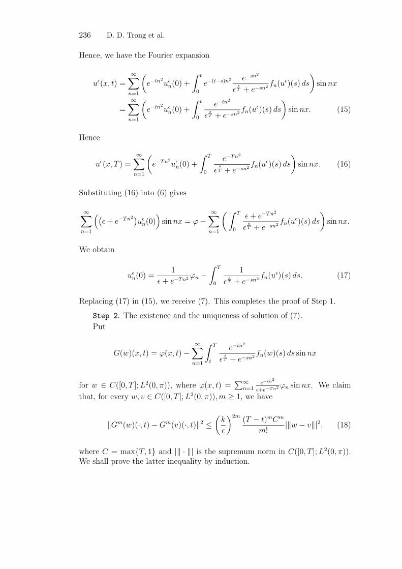
Hence, we have the Fourier expansion
uε(x, t) =∞∑
n=1
(
e−tn2
uεn(0) +
∫ t
0
e−(t−s)n2 e−sn2
εsT + e−sn2
fn(uε)(s) ds
)
sinnx
=∞∑
n=1
(
e−tn2
uεn(0) +
∫ t
0
e−tn2
εsT + e−sn2
fn(uε)(s) ds
)
sinnx. (15)
Hence
uε(x, T ) =∞∑
n=1
(
e−Tn2
uεn(0) +
∫ T
0
e−Tn2
εsT + e−sn2
fn(uε)(s) ds
)
sinnx. (16)
Substituting (16) into (6) gives
∞∑
n=1
(
(
ε+ e−Tn2)
uεn(0))
sinnx = ϕ−∞∑
n=1
(∫ T
0
ε+ e−Tn2
εsT + e−sn2
fn(uε)(s) ds
)
sinnx.
We obtain
uεn(0) =1
ε+ e−Tn2ϕn −
∫ T
0
1
εsT + e−sn2
fn(uε)(s) ds. (17)
Replacing (17) in (15), we receive (7). This completes the proof of Step 1.
Step 2. The existence and the uniqueness of solution of (7).
Put
G(w)(x, t) = ϕ(x, t)−∞∑
n=1
∫ T
t
e−tn2
εsT + e−sn2
fn(w)(s) ds sinnx
for w ∈ C([0, T ];L2(0, π)), where ϕ(x, t) =∑∞
n=1e−tn2
ε+e−Tn2ϕn sinnx. We claim
that, for every w, v ∈ C([0, T ];L2(0, π)),m ≥ 1, we have
‖Gm(w)(·, t)−Gm(v)(·, t)‖2 ≤(
k
ε
)2m(T − t)mCm
m!|‖w − v‖|2, (18)
where C = max{T, 1} and |‖ · ‖| is the supremum norm in C([0, T ];L2(0, π)).We shall prove the latter inequality by induction.
1-D Backward Heat Problem 237
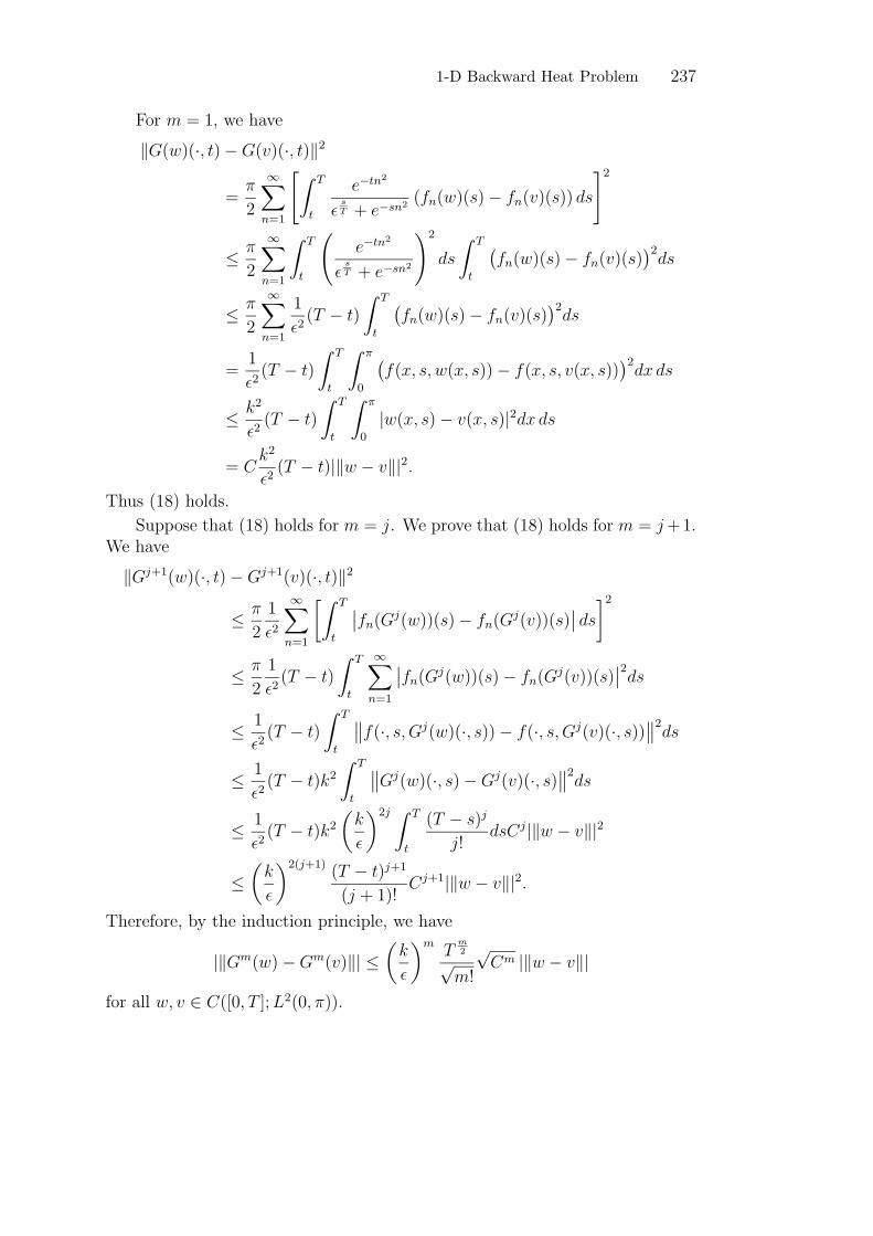
For m = 1, we have
‖G(w)(·, t)−G(v)(·, t)‖2
=π
2
∞∑
n=1
[
∫ T
t
e−tn2
εsT + e−sn2
(fn(w)(s)− fn(v)(s)) ds
]2
≤ π
2
∞∑
n=1
∫ T
t
(
e−tn2
εsT + e−sn2
)2
ds
∫ T
t
(
fn(w)(s)− fn(v)(s))2ds
≤ π
2
∞∑
n=1
1
ε2(T − t)
∫ T
t
(
fn(w)(s)− fn(v)(s))2ds
=1
ε2(T − t)
∫ T
t
∫ π
0
(
f(x, s, w(x, s))− f(x, s, v(x, s)))2dx ds
≤ k2
ε2(T − t)
∫ T
t
∫ π
0
|w(x, s)− v(x, s)|2dx ds
= Ck2
ε2(T − t)|‖w − v‖|2.
Thus (18) holds.
Suppose that (18) holds for m = j. We prove that (18) holds for m = j+1.We have
‖Gj+1(w)(·, t)−Gj+1(v)(·, t)‖2
≤ π
2
1
ε2
∞∑
n=1
[∫ T
t
∣
∣fn(Gj(w))(s)− fn(G
j(v))(s)∣
∣ ds
]2
≤ π
2
1
ε2(T − t)
∫ T
t
∞∑
n=1
∣
∣fn(Gj(w))(s)− fn(G
j(v))(s)∣
∣
2ds
≤ 1
ε2(T − t)
∫ T
t
∥
∥f(·, s, Gj(w)(·, s))− f(·, s, Gj(v)(·, s))∥
∥
2ds
≤ 1
ε2(T − t)k2
∫ T
t
∥
∥Gj(w)(·, s)−Gj(v)(·, s)∥
∥
2ds
≤ 1
ε2(T − t)k2
(
k
ε
)2j ∫ T
t
(T − s)j
j!dsCj|‖w − v‖|2
≤(
k
ε
)2(j+1)(T − t)j+1
(j + 1)!Cj+1|‖w − v‖|2.
Therefore, by the induction principle, we have
|‖Gm(w)−Gm(v)‖| ≤(
k
ε
)mT
m2
√m!
√Cm |‖w − v‖|
for all w, v ∈ C([0, T ];L2(0, π)).
238 D. D. Trong et al.
We considerG : C([0, T ];L2(0, π))→ C([0, T ];L2(0, π)). There exists a pos-
itive integer m0 such that Gm0 is a contraction since limm→∞
(
kε
)m Tm2√Cm√
m!=
0. It follows that the equation Gm0(w) = w has a unique solution uε ∈C([0, T ];L2(0, π)). In fact, one has G(Gm0(uε)) = G(uε). Hence Gm0(G(uε)) =G(uε). By the uniqueness of the fixed point of Gm0 , one has G(uε) = uε, i.e.,the equation G(w) = w has a unique solution uε ∈ C([0, T ];L2(0, π)). FromPart A, Step 1, we complete the proof of Step 2.
Step 3. The solution of the problem (4)−(6) depends continuously on ϕ inL2(0, π).
Let u and v be two solutions of (4)−(6) corresponding to the final values ϕand ω. From (7) one has in view of the inequality (a+ b)2 ≤ 2(a2 + b2)
‖u(·, t)− v(·, t)‖2 ≤ π
∞∑
n=1
(
e−tn2
ε+ e−Tn2|ϕn − ωn|
)2
+ π∞∑
n=1
(∫ T
t
e−tn2
εsT + e−sn2
∣
∣fn(u)(s)− fn(v)(s)∣
∣ds
)2
.
(19)
One has, for s > t and α > 0, e−tn2
α+e−sn2 =1
(αesn2+1)
ts (α+e−sn2
)1−ts≤ α
ts−1. Letting
α = ε, s = T , we get
e−tn2
ε+ e−Tn2≤ ε
tT−1. (20)
Letting α = εsT , we get
e−tn2
εsT + e−sn2
≤ εtT− s
T . (21)
Hence, from (19) it follows that
‖u(·, t)− v(·, t)‖2 ≤ 2ε2( tT−1)‖ϕ− ω‖2
+ 2k2(T − t)ε2tT
∫ T
t
ε−2 sT ‖u(·, s)− v(·, s)‖2ds.
So, we have
ε−2( tT
)‖u(·, t)− v(·, t)‖2 ≤ 2ε−2‖ϕ− ω‖2
+ 2k2(T − t)
∫ T
t
ε−2 sT ‖u(·, s)− v(·, s)‖2ds.
Using Gronwall’s inequality we have
‖u(·, t)− v(·, t)‖ ≤ 2ε tT−1 exp
(
k2(T − t)2)
‖ϕ− ω‖.This completes the proof of Step 3 and the proof of our theorem.
1-D Backward Heat Problem 239
3. Regularization of problem (1)−(3)
We first have a uniqueness result
Theorem 3.1. Let ϕ, f be as in Theorem 2.1. Then problem (1)−(3) has atmost one (weak) solution u ∈W , where
W = C([0, T ];L2(0, π)) ∩ L2(0, T ;H10 (0, π)) ∩ C1((0, T );L2(0, π)).
Proof. Let M > 0 be such that |∂f∂z(x, t, z)| ≤ M for all (x, t, z) ∈ (0, π) ×
(0, T ) × R. Let u1(x, t) and u2(x, t) be two solutions of problem (1)−(3) suchthat u1, u2 ∈W.
Put w(x, t) = u1(x, t)− u2(x, t). Then w satisfies the equation
wt(x, t)− wxx(x, t) = f(x, t, u1(x, t))− f(x, t, u2(x, t)).
Since f is Lipschizian, we have (wt−wxx)2 ≤M2w2. Now w(0, t) = w(π, t) = 0
and w(x, T ) = 0. Hence by the Lees–Protter theorem ([8, p. 373]), w = 0 whichgives u1(x, t) = u2(x, t) for all t ∈ [0, T ]. The proof is completed.
Despite the uniqueness, problem (1)−(3) is still ill-posed. Hence, a regular-ization has to resort. We have the following result.
Theorem 3.2. Let ϕ, f, uε be as in Theorem 2.1.
a) If we can find a u and a subsequence (uεj) in (C[0, T ];L2(0, π)) such that
uεj → u in C([0, T ];L2(0, π)),
then u is the unique solution of Problem (1)−(3).b) If problem (1)−(3) has a weak solution
u ∈W (defined in Theorem 3.1)
which satisfies∫ T
0
∑∞n=1 e
2sn2
f 2n(u)(s)ds <∞. Then
‖u(·, t)− uε(·, t)‖ ≤√M exp
(
3k2T (T − t)
2
)
εtT
for every t ∈ [0, T ], where M = 3‖u(0)‖2 + 6π∫ T
0
∑∞n=1 e
2sn2
f 2n(u)(s)ds
and uε is the unique solution of problem (4)−(6).Proof. a) We present an outline of the proof.
The function uεj satisfies (4), (5) (with ε replaced by εj) subject to theinitial condition uεj(x, 0) =
∑∞n=1 ϕ
jn sinnx and u(x, 0) =
∑∞n=1 un(0) sinnx.
One gets (see [5])
uεj(x, t) =∞∑
n=1
[
e−tn2
ϕjn +
∫ t
0
e−tn2
εs/Tj + e−sn2
fn(uεj)ds
]
sinnx.
240 D. D. Trong et al.
Letting ε ↓ 0, we shall get
u(x, t) =∞∑
n=1
(
e−tn2
un(0) +
∫ t
0
e−(t−s)n2
fn(u) ds
)
sinnx.
On the other hand, letting ε ↓ 0 in (6), we get u(x, T ) = ϕ(x). Hence u is thesolution of problem (1)–(3) as desired.
b) The exact solution u satisfies
u(x, t) =∞∑
n=1
(
e−(t−T )n2
ϕn −∫ T
t
e−(t−s)n2
fn(u)(s) ds
)
sinnx (22)
u(x, T ) =∞∑
n=1
(
e−Tn2
un(0) +
∫ T
0
e−(T−s)n2
fn(u)(s)ds
)
sinnx =∞∑
n=1
ϕn sinnx,
where we recall un(0) =2π〈u(x, 0), sinnx〉 (see [5]). Hence
e−Tn2
un(0) +
∫ T
0
e−(T−s)n2
fn(u)(s) ds = ϕn. (23)
From (7), (22) and (23), we get
|un(t)− uεn(t)| =∣
∣
∣
∣
εe−tn2
e−Tn2(ε+ e−Tn2)
ϕn −∫ T
t
εsT e−tn
2
e−sn2(ε
sT + e−sn2)
fn(u)(s) ds
−∫ T
t
e−tn2
εsT + e−sn2
(
fn(u)(s)− fn(uε)(s)
)
ds
∣
∣
∣
∣
≤∣
∣
∣
∣
εe−tn2
ε+ e−Tn2un(0) +
∫ T
0
εe−tn2
e−sn2(ε+ e−Tn2)
fn(u)(s) ds
−∫ T
t
εsT e−tn
2
e−sn2(ε
sT + e−sn2)
fn(u(s)ds
∣
∣
∣
∣
+
∫ T
t
e−tn2
εsT + e−sn2
∣
∣fn(u)(s)− fn(uε)(s)
∣
∣ds.
(24)
From (20), (21) and (24), we have
|un(t)− uεn(t)|
≤ ε · ε tT−1|un(0)|+
∫ T
0
ε · ε tT−1
∣
∣
∣
∣
fn(u)(s)
e−sn2
∣
∣
∣
∣
ds+
∫ T
t
εsT .ε
tT− s
T
∣
∣
∣
∣
fn(u)(s)
e−sn2
∣
∣
∣
∣
ds
+
∫ T
t
εtT− s
T
∣
∣fn(u)(s)− fn(uε)(s)
∣
∣ds
≤ εtT |un(0)|+ 2ε
tT
∫ T
0
∣
∣
∣
∣
fn(u)(s)
e−sn2
∣
∣
∣
∣
ds+ εtT
∫ T
t
ε−sT
∣
∣fn(u)(s)− fn(uε)(s)
∣
∣ds.
1-D Backward Heat Problem 241
We have in view of the inequality (a+ b+ c)2 ≤ 3(a2 + b2 + c2)
‖u(·, t)− uε(·, t)‖2 =π
2
∞∑
n=1
|un(t)− uεn(t)|2
≤ 3π2
∞∑
n=1
ε2tT |un(0)|2 + 6π
∞∑
n=1
ε2tT
(∫ T
0
∣
∣
∣
1
e−sn2fn(u)(s)
∣
∣
∣ds
)2
+3π
2
∞∑
n=1
ε2tT
(∫ T
t
ε−sT
∣
∣fn(u)(s)− fn(uε)(s)
∣
∣ds
)2
≤ 3ε2 tT ‖u(0)‖2 + 6πTε2
tT
∫ T
0
∞∑
n=1
e2sn2
f 2n(u)(s) ds
+ 3(T − t)ε2tT
∫ T
t
ε−2 sT ‖f(·, s, u(·, s))− f(·, s, uε(·, s))‖2ds
≤ ε2tT
(
3‖u(0)‖2 + 6πT
∫ T
0
∞∑
n=1
e2sn2
fn(u(s))2ds
+ 3k2T
∫ T
t
ε−2 sT ‖u(·, s)− uε(·, s)‖2ds
)
.
Hence
ε−2 tT ‖u(·, t)− uε(·, t)‖2 ≤M + 3k2T
∫ T
t
ε−2 sT ‖u(·, s)− uε(·, s)‖2ds ,
whereM = 3‖u(0)‖2+6πT∫ T
0
∑∞n=1 e
2sn2
f 2n(u)(s)ds. Using Gronwall’s inequal-
ity, we get
ε−2 tT ‖u(·, t)− uε(·, t)‖2 ≤Me3k2T (T−t).
This completes the proof of Theorem 3.2.
Remark 3.3.1. From Part a), we conclude that if problem (1)−(3) does not have any
exact solution u ∈ W , then one has
limε↓0inf{
max0≤t≤T
‖uε(·, t)− ψ(·, t)‖}
> 0
for every ψ ∈ C([0, T ];L2(0, π)).2. If f(x, t, u) ≡ 0, we have the linear homogeneous problem, the error
estimate is as in [2].3. From (23), one has
un(0) = ϕneTn2 −
∫ T
0
esn2
fn(u)(s)ds .
242 D. D. Trong et al.
If∑∞
n=1 ϕ2ne
2Tn2
< ∞, then∑∞
n=1
( ∫ T
0esn
2
fn(u)(s)ds)2
< ∞. Hence the as-sumptions of f in Theorem 3.2 are reasonable.
One has
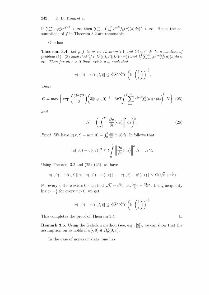
Theorem 3.4. Let ϕ, f be as in Theorem 2.1 and let u ∈ W be a solution ofproblem (1)−(3) such that ∂u
∂t∈L2((0, T );L2(0, π)) and
∫ T
0
∑∞n=1e
2sn2
f 2n(u)(s)ds<
∞. Then for all ε > 0 there exists a tε such that
‖u(·, 0)− uε(·, tε)‖ ≤ 4√8C
4√T
(
ln
(
1
ε
))− 1
4
,
where
C = max
{
exp
(
3k2T 2
2
)(
3‖u0(·, 0)‖2+ 6πT
∫ T
0
∞∑
n=1
e2sn2
f 2n(u)(s)ds
)1
2
, N
}
(25)
and
N =
(∫ T
0
∥
∥
∥
∥
∂u
∂t(·, s)
∥
∥
∥
∥
2
ds
)1
2
. (26)
Proof. We have u(x, t)− u(x, 0) =∫ t
0∂u∂s(x, s)ds. It follows that
‖u(·, 0)− u(·, t)‖2 ≤ t
t∫
0
∥
∥
∥
∥
∂u
∂t(·, s)
∥
∥
∥
∥
2
ds = N 2t.
Using Theorem 3.2 and (25)–(26), we have
‖u(·, 0)− uε(·, t)‖ ≤ ‖u(·, 0)− u(·, t)‖+ ‖u(·, t)− uε(·, t)‖ ≤ C(√t+ ε
tT ).
For every ε, there exists tε such that√tε = ε
tεT , i.e., ln tε
tε= 2 ln ε
T. Using inequality
ln t > −1tfor every t > 0, we get
‖u(·, 0)− uε(·, tε)‖ ≤ 4√8C
4√T
(
ln
(
1
ε
))− 1
4
.
This completes the proof of Theorem 3.4.
Remark 3.5. Using the Galerkin method (see, e.g., [9]), we can show that theassumption on ut holds if u(·, 0) ∈ H1
0 (0, π).
In the case of nonexact data, one has
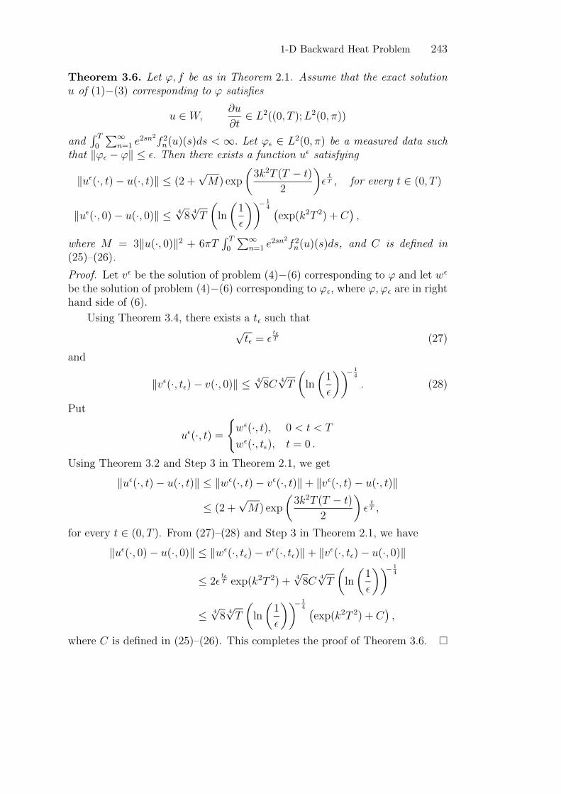
1-D Backward Heat Problem 243
Theorem 3.6. Let ϕ, f be as in Theorem 2.1. Assume that the exact solutionu of (1)−(3) corresponding to ϕ satisfies
u ∈ W, ∂u
∂t∈ L2((0, T );L2(0, π))
and∫ T
0
∑∞n=1 e
2sn2
f 2n(u)(s)ds < ∞. Let ϕε ∈ L2(0, π) be a measured data such
that ‖ϕε − ϕ‖ ≤ ε. Then there exists a function uε satisfying
‖uε(·, t)− u(·, t)‖ ≤ (2 +√M) exp
(
3k2T (T − t)
2
)
εtT , for every t ∈ (0, T )
‖uε(·, 0)− u(·, 0)‖ ≤ 4√8
4√T
(
ln
(
1
ε
))− 1
4(
exp(k2T 2) + C)
,
where M = 3‖u(·, 0)‖2 + 6πT∫ T
0
∑∞n=1 e
2sn2
f 2n(u)(s)ds, and C is defined in
(25)–(26).
Proof. Let vε be the solution of problem (4)−(6) corresponding to ϕ and let wε
be the solution of problem (4)−(6) corresponding to ϕε, where ϕ, ϕε are in righthand side of (6).
Using Theorem 3.4, there exists a tε such that√tε = ε
tεT (27)
and
‖vε(·, tε)− v(·, 0)‖ ≤ 4√8C
4√T
(
ln
(
1
ε
))− 1
4
. (28)
Put
uε(·, t) ={
wε(·, t), 0 < t < T
wε(·, tε), t = 0 .
Using Theorem 3.2 and Step 3 in Theorem 2.1, we get
‖uε(·, t)− u(·, t)‖ ≤ ‖wε(·, t)− vε(·, t)‖+ ‖vε(·, t)− u(·, t)‖
≤ (2 +√M) exp
(
3k2T (T − t)
2
)
εtT ,
for every t ∈ (0, T ). From (27)–(28) and Step 3 in Theorem 2.1, we have‖uε(·, 0)− u(·, 0)‖ ≤ ‖wε(·, tε)− vε(·, tε)‖+ ‖vε(·, tε)− u(·, 0)‖
≤ 2ε tεT exp(k2T 2) +
4√8C
4√T
(
ln
(
1
ε
))− 1
4
≤ 4√8
4√T
(
ln
(
1
ε
))− 1
4(
exp(k2T 2) + C)
,
where C is defined in (25)–(26). This completes the proof of Theorem 3.6.
244 D. D. Trong et al.
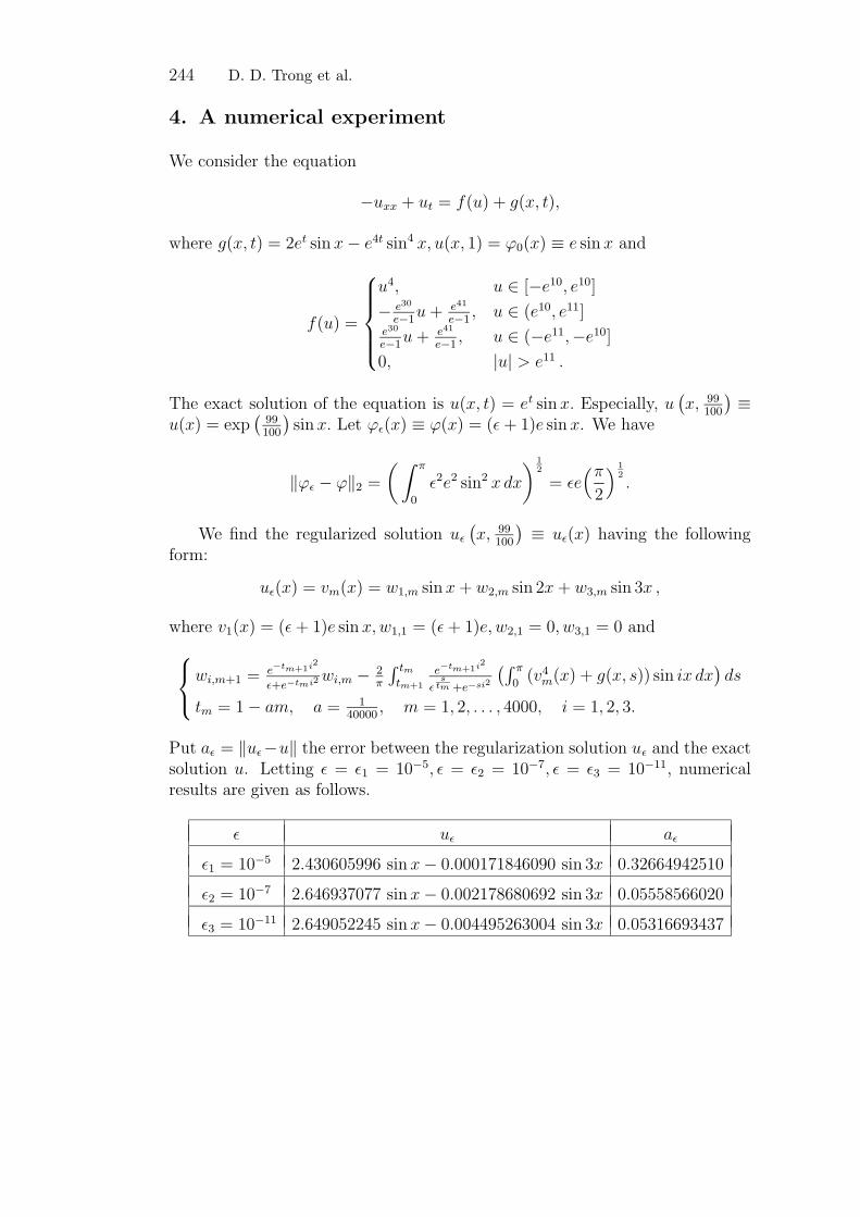
4. A numerical experiment
We consider the equation
−uxx + ut = f(u) + g(x, t),
where g(x, t) = 2et sinx− e4t sin4 x, u(x, 1) = ϕ0(x) ≡ e sinx and
f(u) =
u4, u ∈ [−e10, e10]
− e30
e−1u+ e41
e−1, u ∈ (e10, e11]
e30
e−1u+ e41
e−1, u ∈ (−e11,−e10]
0, |u| > e11 .
The exact solution of the equation is u(x, t) = et sinx. Especially, u(
x, 99100
)
≡u(x) = exp
(
99100
)
sinx. Let ϕε(x) ≡ ϕ(x) = (ε+ 1)e sin x. We have
‖ϕε − ϕ‖2 =
(∫ π
0
ε2e2 sin2 x dx
)1
2
= εe(π
2
)1
2
.
We find the regularized solution uε(
x, 99100
)
≡ uε(x) having the followingform:
uε(x) = vm(x) = w1,m sinx+ w2,m sin 2x+ w3,m sin 3x ,
where v1(x) = (ε+ 1)e sinx,w1,1 = (ε+ 1)e, w2,1 = 0, w3,1 = 0 and
wi,m+1 =e−tm+1i
2
ε+e−tmi2wi,m − 2
π
∫ tmtm+1
e−tm+1i2
εs
tm +e−si2
(∫ π
0(v4
m(x) + g(x, s)) sin ix dx)
ds
tm = 1− am, a = 140000
, m = 1, 2, . . . , 4000, i = 1, 2, 3.
Put aε = ‖uε−u‖ the error between the regularization solution uε and the exactsolution u. Letting ε = ε1 = 10
−5, ε = ε2 = 10−7, ε = ε3 = 10
−11, numericalresults are given as follows.
ε uε aε
ε1 = 10−5 2.430605996 sin x− 0.000171846090 sin 3x 0.32664942510
ε2 = 10−7 2.646937077 sin x− 0.002178680692 sin 3x 0.05558566020
ε3 = 10−11 2.649052245 sin x− 0.004495263004 sin 3x 0.05316693437
1-D Backward Heat Problem 245
Acknowledgement. The authors wish to thank the referee for their valuablecriticisms and suggestions, leading to the present improved version of our paper.
References
[1] Alekseeva, S. M. and Yurchuk, N. I., The quasi-reversibility method for theproblem of the control of an initial condition for the heat equation with anintegral boundary condition. Diff. Equations 34 (1998)(4), 493 – 500.
[2] Ames, K. A., Clark, G. W., Epperson, J. F., Oppenheimer, S. F., A comparisonof regularizations for an ill-posed problem. Math. Comp. 67 (1998), no.224,1451 – 1471.
[3] Ames, K. A. and Payne, L. E., Continuous dependence on modeling for somewell-posed perturbations of the backward heat equation. J. Inequal. Appl. 3(1999)(1), 51 – 64.
[4] Clark, G. and Oppenheimer, C., Quasireversibility methods for non-well-posedproblem. Electron. J. Diff. Equations 8 (1994), 1 – 9.
[5] Colton, D., Partial Differential Equations. New York: Random House 1988.
[6] Denche, M. and Bessila, K., Quasi-boundary value method for non-well posedproblem for a parabolic equation with integral boundary condition. Math.
Probl. Eng. 7 (2001)(2), 129 – 145.
[7] Lattes, R. and Lions, J. L., Methode de Quasi-Reversibilite et Applications.
Paris: Dunod 1967.
[8] Lees, M. and Protter, M. H., Unique continuation for parabolic differentialequations and inequalities. Duke Math. J. 28 (1961), 369 – 382.
[9] Lions, J. L., Quelques methodes de resolution des problemes aux limites non-
lineaires (in French). Paris: Dunod, Gauthier-Villars 1969.
[10] Miller, K., Stabilized quasi-reversibility and other nearly-best-possible methodsfor non-well-posed problems. Symposium on Non-Well-Posed Problems and
Logarithmic Convexity (Heriot-Watt Univ., Edinburgh 1972; ed.: R. J. Knops).Lecture Notes Math. 316. Berlin: Springer 1973, pp. 161 – 176.
[11] Quan, P. H. and Dung, N., A backward nonlinear heat equation: regularizationwith error estimates, Appl. Anal. 84 (2005)(4), 343 – 355.
[12] Showalter, R. E., Quasi-reversibility of first and second order parabolic evo-lution equations. Improperly Posed Boundary Value Problems (Conf., Univ.New Mexico, Albuquerque, N. M., 1974; eds.: A. Carasso and A. P. Stone).Res. Notes Math. 1. London: Pitman 1975, pp. 76 – 84.
Received May 29, 2005; revised February 13, 2006