A new three-dimensional CFD model for efficiency ...

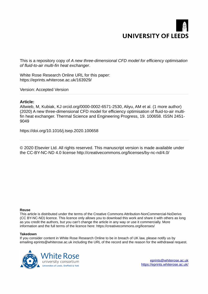
This is a repository copy of A new three-dimensional CFD model for efficiency optimisationof fluid-to-air multi-fin heat exchanger.

White Rose Research Online URL for this paper:https://eprints.whiterose.ac.uk/163929/

Version: Accepted Version

Article:

Altwieb, M, Kubiak, KJ orcid.org/0000-0002-6571-2530, Aliyu, AM et al. (1 more author) (2020) A new three-dimensional CFD model for efficiency optimisation of fluid-to-air multi-fin heat exchanger. Thermal Science and Engineering Progress, 19. 100658. ISSN 2451-9049

https://doi.org/10.1016/j.tsep.2020.100658

© 2020 Elsevier Ltd. All rights reserved. This manuscript version is made available under the CC-BY-NC-ND 4.0 license http://creativecommons.org/licenses/by-nc-nd/4.0/

[email protected]://eprints.whiterose.ac.uk/

Reuse

This article is distributed under the terms of the Creative Commons Attribution-NonCommercial-NoDerivs (CC BY-NC-ND) licence. This licence only allows you to download this work and share it with others as long as you credit the authors, but you can’t change the article in any way or use it commercially. More information and the full terms of the licence here: https://creativecommons.org/licenses/

Takedown

If you consider content in White Rose Research Online to be in breach of UK law, please notify us by emailing [email protected] including the URL of the record and the reason for the withdrawal request.

Preprint version of M. Altwieb, K.J. Kubiak, A.M. Aliyu, R. Mishra, A new three-dimensional CFD model for efficiency optimisation of fluid-to-air multi-

fin heat exchanger, Thermal Science and Engineering Progress (2020) Vol. 19, 100658, Elsevier, DOI: 10.1016/j.tsep.2020.100658

A new three-dimensional CFD model for efficiency optimisation of fluid-

to-air multi-fin heat exchanger

Miftah Altwieb1, Krzysztof J. Kubiak 2, Aliyu M. Aliyu3, Rakesh Mishra 3

1Department of Mechanical and Industrial Engineering, University of Gharyan, Libya 2School of Mechanical Engineering, University of Leeds, United Kingdom

3School of Computing and Engineering, University of Huddersfield, United Kingdom

Abstract

New simulation and experimental results have been obtained and are presented for a multi-tube

fin heat exchanger unit, from which semi-analytical correlations for the Fanning friction and Colburn

factors were developed. The multi-tube and fin heat exchanger represents the main component of

the Fan Coil Unit, an essential component of HVAC systems used for domestic and commercial

heating and cooling. Improving the efficiency of the heat exchanger typically comes at the expense

of higher pressure drops or costlier materials and production costs. Here, an experimental setup

was designed and constructed to evaluate the thermal performance of such a heat exchanger.

Geometrical modifications were explored for thermal performance enhancement. Furthermore, full

three-dimensional CFD case studies of the heat exchanger were investigated to examine the effect

of the geometrical features on the air side of the heat exchanger to study the effect of fin spacing,

transverse and longitudinal pitches. The CFD model developed was first globally validated against

experimental results. The model results were used to predict the Fanning and Colburn factors and

the local fin efficiency based on the carefully selected geometric parameters. The data obtained was

utilised to develop two new semi-analytical models for the Fanning and Colburn friction factors

which were well within ±10% error bands and showed strong correlation coefficients of more than

98 and 97% respectively.

Key Words: CFD modelling, Colburn factor, Fanning friction factor, fin efficiency, heat exchangers.

1 INTRODUCTION

There is an undoubted increase in global demand for heating and cooling of residential and

industrial buildings. This in turn leads to a rapid increase in the CO2 footprint due to commercial and

domestic heating and cooling. Climate scientists have warned of the environmental impact of

human activities fast approaching an irreversible point, that will create a permanent change to the

planet’s natural environment. Therefore, increasing the efficiency of Heating, Ventilation and Air

Conditioning (HVAC) systems will undoubtedly have a significant impact on achieving net zero

carbon goals set by governments around the world. For example, the UK government is aiming to

achieve net zero carbon emission target by 2050 [1]. Improving the efficiency of energy systems

including HVAC devices such as fan and coil units is key to achieving this target. A Fan Coil Unit (FCU)

mainly consists of a heating or cooling coil and a fan. Normally, an FCU is coupled to the pipework

for controlling the temperature in the installed space [2].

Cavallini et al. [3] reported work carried out on a HVAC system with smooth tubes where the

behaviour of pure/blended halogenated and high-pressure hydrofluorocarbons (HFC) was studied.

The heat transfer coefficient as well as the pressure drop characteristics during condensation were

investigated. They proposed a new predicting model based on the flow patterns that occur during

the condensation process. They showed that predictions from their model agreed with a large

experimental data bank from the literature. While their work and others in the literature are

important work, the awareness on climate change and global warming means that further research

into more sustainable refrigerants for HVAC systems is needed.




For example, [4] report an innovative use of the traditional Shavadoon HVAC system via a numerical

study. It uses natural convection and their results showed that it has the ability to reduce radically

reduce the ambient temperature and maintain comfort conditions. They varied the system’s

geometrical parameters e.g. valve at the canal outlet, its location and diameter and concluded that

using an S-shaped intake with an exit controlling valve improved the ventilation without

deteriorating the thermal comfort conditions. Therefore, it can effectively decrease energy

consumption and prevent possible environmental damage caused by conventional HVAC systems

that use HFCs and other refrigerants that have been shown to have adverse effects on the

environment.

Numerous studies have been carried out reporting various improvement schemes for the efficiency

of FCUs and other heat exchanger systems in order to handle a certain heating or cooling duty. In

general, techniques of augmentation or enhancement are divided into active, where external forces

are employed to enhance heat transfer characteristics; and passive techniques, which use surface

or geometric adjustments to the flow channel by using inserts or additional tools. Alternatively,

combining passive and active methods can be used to further boost a heat exchanger's thermo-

hydraulic performance [5].

Wang and Chi [6] examined the air-side efficiency of fine and tube heat exchangers with the

configuration of a simple fin. Eighteen samples were studied to analyse the effect on thermal and

flow characteristics of the number of fin spacing, number of tube rows, and the tube diameter. It

was concluded that for a Reynolds number range i.e. 𝑅𝑒 = 300–3000, and for one and two tube

rows, the fin pitch clearly influences the heat transfer behaviour. In addition, a very small influence

of the number of rows was noticed on the friction performance and the influence of the tube

diameter on the heat transfer output is related to the fin pitch, which was consistent with the results

reported in their earlier study [7]. For a louvered fin-and-tube heat exchanger without louvre

redirection, Wang et al. [8] experimentally found that that the friction factors are unaffected by the

number of tube rows, more so at 𝑅𝑒 > 2000 and the heat transfer coefficients were found to

significantly reduce at conditions of 𝑅𝑒 < 2000 in the case of the six-row coil heat exchanger they

studied. Furthermore, they discovered that the maximum j factor values occur at lower 𝑅𝑒 values

and this corresponds to lower fin spacing and vortex formation; and that fin pitch does not affect

the characteristics of heat transfer at 𝑅𝑒 > 2000. However, heat transfer coefficients are directly

proportional to fin pitch. They finally derived a correlation for the Colburn and Fanning factors that

described the data to with a 10% error band.

An experimental investigation of a compact heat exchanger unit was carried out by Shinde and Lin

[9]. The fins were fitted with louvers and flat tubes and the air-side 𝑅𝑒 range was 20–200.

Experiments were carried out with twenty-six different corrugated louvered-fin heat exchangers.

The data collected was used to derive correlations for the j and f factors in two Reynolds number

ranges namely 𝑅𝑒 = 20–80 and 𝑅𝑒 = 80–200. They concluded that airflow and heat transfer

characteristics are different at very low and high Reynolds numbers. It is noted that their Reynolds

number range is rather narrow and cannot be applied for applications with requirements of high

flow throughput.

Taler [10] proposed two methods for calculating the coefficient heat transfer on the air side for a

two-pass radiator consisting of two aligned rows of oval-shaped tubes having flat, simple fins. They

obtained a correlation for the air-side heat transfer coefficient using experimental data. In addition,

they inferred that the heat transfer coefficients are greater based on the difference in air

temperature through the heat exchanger determined using the latter approach i.e. computational

fluid dynamics (CFD). This is because their CFD model does not consider conductance caused by the

thermal interaction between the pipes and fins. Dong et al. [11] reported an experimental and CFD




study of pressure loss and thermal performance for airflow through a wavy fin in the fully-developed

turbulent regime. The wavy fin profiles they used are: triangular round corner, sinusoidal and

triangular. Findings of this investigation suggested the wavy fin profiles had almost no effect on f

and heat transfer efficiency. They also stated that the standard 𝑘 − 𝜀 turbulence model was the

most appropriate for simulating air flow and heat transfer of their wavy fin configurations for the

range of 𝑅𝑒 = 1000 to 5500.

While experimental studies are most desirable, there can be huge costs involved in setting them up

especially if several configurations are to be examined. As a result, numerical research on fin and

tube heat exchangers has recently been done using CFD. It is noted that the reported works have a

rather restricted range of factors examined with most CFD studies using a computational framework

that takes only part of the fin into account. Furthermore, most of these studies neglect local flow

distribution analysis, such as those of temperature, heat transfer coefficient, as well as the local fin

efficiency of working fluids and fins. Identifying the improvement of these local flow characteristics

can improve the efficiency of the heat exchanger.

Lu et al. [12] investigated the geometrical features on the performance of a fin-and-tube heat

exchanger with six tube rows for refrigerator applications. They studied the effects of tube pitch, its

diameter, fin pitch, and their thickness. They measured the heat exchanger performance in terms

of the ratio of heat transfer rate to pressure drop as well as the coefficient of performance. It was

found that performance increased with longitudinal and transverse tube pitch, but it decreased with

tube diameter and fin thickness. However, the study was carried out on a partial heat exchanger

geometry, and the effect of the different geometrical parameters cannot be confidently

extrapolated to model the behaviour of the full heat exchanger geometry. The same can be said for

the study of Lin et al. [13] where they reported a CFD investigation over a staggered circular tube

bank fin heat exchanger with an interrupted half annular groove fin. They observed that at lower

Reynolds numbers, the fin surface did not significantly affect heat transfer but much better

performance was achieved at higher Reynolds numbers. There was a mean increase of 10–40% in

the f factor and Nusselt number of the annular groove fin was obtained in comparison to that of the

baseline plain fin with heat transfer performance increasing 7.0% to 27.0% when 𝑅𝑒 increased from

600 to 2500 respectively. Again, their work was on part of the heat exchanger geometry and little

or no information can be inferred for the full thermal characteristics of the heat exchanger.

In a CFD study, Čarija et al. [14] analysed air-side flow of a fin and tube heat exchanger having

multiple rows with flat and louvered. An 𝑅𝑒 range of 70–350, calculated using fin spacing and front

air velocities, was used. They showed that there was improved heat transfer performance of nearly

60% for the louvered fins at 𝑅𝑒 = 350 in comparison to flat fins. Additionally, as the length of the

louvre increases, the heat transfer efficiency proportionally increased for the same Reynolds

numbers. Altwieb et al. [15] performed a CFD study with benchmarking experiments to measure

performance characteristics of a multi-tube and fin heat exchanger at steady state. A three-

dimensional computational model with complete heat exchanger geometry was developed. They

explored the performance of several fin configurations: louvered, semi-dimpled vortex generator,

and plain. The results showed that the thin vortex generator fins produced the highest non-

dimensional heat transfer parameter hence best performance of the fin configurations studied. Two

dimensionless empirical equations were derived from the simulation data. They suggested that the

relationships can be used for sizing and design of the heat exchangers to estimate the rate of heat

transfer and the pressure characteristics on the air side.


Preprint version of M. Altwieb, K.J. Kubiak, A.M. Aliyu, R. Mishra, A new three-dimensional CFD model for efficiency optimisation of fluid-to-air multi-fin heat exchanger, Thermal Science and Engineering Progress (2020) Vol.

19, 100658, Elsevier, DOI: 10.1016/j.tsep.2020.100658

(b)

(c)

(a) (d)

Figure 1: Schematic showing (a) overall experiment Setup (b) heat Exchanger testing unit (c) heat exchanger dimensions (in mm) (d) image of fin heat exchanger




The current investigation presents a qualitative as well as quantitative evaluation of a full-geometry

fin and multi-tube heat exchanger having plain fins. A number of numerical simulations were carried

out which were well-validated with experimental measurements. The analysis carried out is

important for understanding the complex flow behaviour of the heat exchanger with plain fins. In

addition, a parametric analysis of geometric features on pressure drop and heat transfer attributes

of the heat exchanger represented by the friction and Colburn factors. We consider steady state

conditions. The data from this study has been used to establish a new set of semi-

empirical correlations that consider the effects of geometric parameters and can be used for the

optimisation of heat exchanger efficiency.

2 EXPERIMENTS

2.1 Experimental Setup

Planning and conducting experiments is an important step in studying the thermal and hydraulic

performance of heat exchanges as they provide vital measurements for the validation of simulation

results. Figure 1 (a) shows the complete experimental setup used to obtain temperature and

pressure differences across the current heat exchanger system at different inlet flow conditions. It

comprises of a water tank, a pump, flow meter, a heat exchanger testing unit, pressure transducers,

a data logger for thermocouples, a data logger for RTD temperature sensors and a windows-based

personal computer. There are a variety of fin types, such as plain, louvered, convex-louvered, and

wavy. Among these designs, the most common fin design in heat exchanger applications is the

simple fin configuration, due to its simplicity and rigidity, and has been used in this work.

Furthermore, circular tubes are common geometries used in such heat exchangers [5]. An

experimental setup was conceptualised, designed and constructed to conduct steady-state

experiments on a multi-tube and fin heat exchanger. Figure 1 (b) presents the schematic diagram of

the heat exchanger test unit. The test unit was manufactured using a 2 mm thick galvanised steel

sheet. The test section’s length is 650 mm, a width of 165 mm and height of 175 mm. It consists mainly of a one-sided centrifugal fan having an integrated electronically-commutated (EC) motor to

drive the ambient air flow through the test unit, the heat exchanger and the following measuring

components.:

• TFI Cobra Probes for air velocity measurement

• Temperature of the inlet and outlet air measurement stations, each of which consists of T-

type exposed welded tip thermocouples made of a Copper–Constantan alloy [6], [16] for the

study of temperature distribution (7 in number)

• Micro-Manometer for the measurement of air-side pressure drop

• Flow Straightener (Honeycomb Structure) for turbulence suppression at the air inlet

The heat exchanger system utilised consists of two rows of tubes with a diameter of 9,52 mm, each

row comprises 5 tubes, with the length of each tube being 130 mm and connected with a bend of

16 mm. Tubes are made of copper with a thickness of 0.26 mm. The heat exchanger consists of

twenty-one staggered plain aluminium fins with a thickness of 0.12 mm. The fins are 43.3 mm apart

and 125.3 mm in height. The fins are spaced 4.23 mm apart (6 fins per inch). Figure 1 (c) shows the

detailed dimensions of the heat exchanger.

2.2 Experimental tests Procedure

Steady state experiments are the simplest type of experiments to conduct and analyse as the flow

is time independent. In the present analysis, experiments were carried out by drawing flow of air

through the fins of the heat exchanger while hot water was flowing in the heat exchanger tubes.

The air velocity used here is within a range of 0.7–5 m/sec, representing the mean velocity of the




airflow across the square duct measured using ASHRAE 41.2 standard [17] and widely reported [18],

[19]. The temperature of the air inlet is 24 ± 1 oC. The water flow rate range is between 2.0 L/min

and 6.0 L/min. Inlet and outlet temperatures were determined by Pico resistance temperature

detector probes (model RTD-PT100) [16]. The temperature of the inlet water was kept constant at

60.0 ± 1 oC.

2.3 Data Analysis

The temperatures at both air and water inlets; and air and water outlets were measured along with

the pressure drop across the water and the air sides. For the heat transfer rate, the effectiveness–number of transfer units (or ε-NTU) method is used. This method is mostly for counter-current heat

exchangers in preference to the log-mean temperature difference (LMTD) method in cases where

there is inadequate information for the calculation of the LMTD. The number of heat transfer units

(NTU) is computed as follows: 𝑁𝑇𝑈 = 𝑈𝐴/Cmin (1) where 𝐶𝑚𝑖𝑛 = 𝑚𝑚𝑖𝑛𝑐𝑝,𝑚𝑖𝑛 with 𝑚𝑚𝑖𝑛 and 𝑐𝑝,𝑚𝑖𝑛 being the mass and specific heat capacity of the

fluid with the lower heat capacity rate (the air side in this case). The air and water side heat transfer

are expressed as: �̇�𝑤 = �̇�𝑤𝐶𝑝𝑤(𝑇𝑤𝑖 − 𝑇𝑤𝑜) (2) �̇�𝑎 = �̇�𝑎𝐶𝑝𝑎(𝑇𝑎𝑜 − 𝑇𝑎𝑖) (3)

In order to minimise any drop in j, data reduction based on the mean rate of heat transfer �̇�𝑎𝑣𝑔 is

done [20]. Therefore, �̇�𝑎𝑣𝑔 can be calculated as follows: �̇�𝑎𝑣𝑔 = �̇�𝑤 + �̇�𝑎2 (4)

The heat exchanger effectiveness (ε) is the ratio of the actual to the maximum achievable heat

transfer rate. As a result, a relationship for ε can be written as: 𝜀 = �̇�𝑎𝑣𝑔𝐶𝑚𝑖𝑛(𝑇𝑤𝑖 − 𝑇𝑎𝑖) (5)

The maximum achievable heat transfer rate is obtained when the temperature difference between

the inlet and outlet streams is at a maximum. The quantity UA, also known as the overall

conductance, is given by [15]: 𝑈𝐴 = 11𝜂𝑜ℎ𝑎𝐴𝑎 + 𝑅𝑤𝑎𝑙𝑙 + 1ℎ𝑤𝐴𝑤 (6)

where ℎ𝑤 and ℎ𝑎 are the water and air heat transfer coefficients respectively; 𝐴𝑤 and Aa are the

heat transfer areas for the water and the air surfaces respectively; and 𝑅𝑤𝑎𝑙𝑙 is the thermal

resistance of the wall. Where a flat wall is involved, the thermal resistance is given as: 𝑅𝑤𝑎𝑙𝑙 = 𝛿𝑤𝑎𝑙𝑙𝑘𝑤𝑎𝑙𝑙𝐴𝑤𝑎𝑙𝑙 (7)

where 𝛿𝑤𝑎𝑙𝑙 is the thickness of the wall, 𝑘𝑤𝑎𝑙𝑙 is the wall material’s thermal conductivity; 𝐴𝑤𝑎𝑙𝑙 is

the wall heat transfer area; and the heat transfer coefficient of the water-side ℎ𝑤 is calculated using

the Gnielinski [21] correlation:



fin heat exchanger, Thermal Science and Engineering Progress (2020) Vol. 19, 100658, Elsevier, DOI: 10.1016/j.tsep.2020.100658 ℎ𝑤 = (𝑘𝐷)𝑤 (𝑅𝑒𝐷𝑤 − 1000)𝑃𝑟 (𝑓𝑖 2⁄ )1 + 12.7√(𝑓𝑖 2⁄ ) (𝑃𝑟2 3⁄ − 1) (8)

Where 𝑓𝑖 is the water–wall friction factor, and it is given by: 𝑓𝑖 = [1.58 𝑙𝑛(𝑅𝑒𝐷𝑤) − 3.28]−2 (9)

The Colburn j and Fanning f factors are calculated from Equations (10) and (11): 𝑗 = ℎ𝑎𝜌𝑎𝑉𝑎(𝑚𝑎𝑥)𝐶𝑝𝑎 Pr2/3 (10)

𝑓 = 𝐴𝑐𝐴𝑜 𝜌𝑚𝜌1 [2𝜌1∆𝑃𝐺𝑐2 − (𝐾𝑖 + 1 − 𝜎2) + (1 − 𝜎2 − 𝐾𝑒) 𝜌1𝜌2 − 2 (𝜌1𝜌2 − 1)] (11)

Equation (11) was derived by Kays and London [22]. Where 𝐾𝐼 and 𝐾𝑒 are the sudden contraction

and expansion pressure loss coefficients respectively, 𝜌1 and 𝜌2, and 𝜌𝑚 are the air inlet, outlet, and

mean air densities respectively; and 𝜎 is the ratio of the smallest flow area to the front area of the

air duct.

3 NUMERICAL SIMULATION MODEL AND NUMERICAL METHODS

3.1 Numerical Simulation Model

Numerical simulations of heat exchanger configurations in this study were performed with the

commercial software code ANSYS FLUENT 17.0 in order to determine the relationship between the

configurations and performance. This was achieved in three stages namely pre-processing, the

solver set up and the post-processing stage [23]. In the pre-processing stage, the geometry of the

heat exchanger and flow domain were created and meshed in Design Modeller and ANSYS Meshing

respectively. These were then imported into FLUENT in order to define the among other things the

material properties, the boundary conditions, select the turbulence model, solution methods, and

convergence criteria. Good theoretical and background knowledge is needed for a particular system

in order to select the correct settings [24]which include spatial and temporal discretisation methods,

the latter in the case of transient simulations. In the present work, time discretisation was not

considered since steady simulations were carried out. The final stage of the modelling process is

post-processing where the data are extracted at appropriate planes and results visualised [25].

Within this section, a novel CFD model including the complete 3D geometry of a single fin heat

exchanger is presented. The heat exchanger design was developed using the commercial ANSYS

Design Modeler software, and is shown in Figure 2. The model was made with the same geometry

and dimensions as the experimental model consisting of 21 fins (4.23 mm apart) and made of

aluminium with each fin having a thickness of 0.12 mm (6 fins per 2.54 mm). The fin was mounted

in a computational domain (of dimensions 65 x 175 x 650 mm), which was divided into three parts

(of dimensions 165 x 175 x 180, 165 x 175 x 60 and 165 x 175 x 410 mm) to help control the mesh

size across the complex geometry of the heat exchanger tubes and fins.

The three-dimensional mass conservation (continuity), momentum and energy equations were

simultaneously solved for the flow and temperature fields. The turbulent flow regime is considered

by reference to the spectrum of experimental Reynolds numbers. The double precision steady-

state solver and the SST k−ω turbulence model [26] were used primarily because it maintains the

characteristics of the k−ω model near the wall and slowly decreases away from the wall to provide

more accurate results [27]. The pressure, density, body force, the energy and momentum under-




relaxation factors used were respectively 0.3, 1.0, 1.0 and 0.7. The 2nd-order upwind discrimination

scheme was used because it gives more accurate results [20] due to the truncation of the Taylor

series to the 2nd term as against to the 1st in first order schemes. Gravitational acceleration was

activated in the minus y-direction. Coupling of interfaces was done. ANSYS FLUENT enables two

different walls to be combined, allowing the solver to compute quantities right from the solution in

adjacent cells [23].

Figure 2: CFD Model for Multi-tube and Fin Heat Exchanger with Plain Fins

According to the ANSYS FLUENT user guide, the command' rpsetvar' (i.e.' temperature / secondary

gradient? #f') should be added to turn off the secondary gradient to aid convergence in areas of low

mesh quality [23] which can be done in regions of highly complex geometry such as those near tube

curvature and between fins. The heat is transmitted through the walls by conduction. The thermal

conductivity of the copper tubes was set at 387.6 W/m.K and the thermal conductivity of the

aluminium fins was set at 202.4 W/m.K. The air and water properties used are as follows: densities 𝜌𝑤𝑎𝑡𝑒𝑟 = 998.2 kg/m3, 𝜌𝑎𝑖𝑟 = 1.24 kg/m3 (set as an incompressible ideal gas [23]); viscosities 𝜇𝑤𝑎𝑡𝑒𝑟 = 0.000471 kg/m.s, 𝜇𝑎𝑖𝑟 = 0.00001789 kg/m.s; and specific heat capacities 𝐶𝑝𝑤𝑎𝑡𝑒𝑟 =4179 J/kg.K, 𝐶𝑝𝑎𝑖𝑟 = 1005.684 J/kg.K.

3.2 Meshing and Mesh Independence Test

A hybrid meshing technique [23] was adopted for the flow domain using tetrahedral (tetra) and

quadrilateral (quad) mesh elements for the test section which was divided into three parts. The

division splits the flow domain into the near field of the heat exchanger sandwiched between the

air inlet and outlet sections. This allows for refining of the mesh to be carried out in the middle

section to give finer mesh elements in the vicinity of the heat exchanger unit. Figure 3 (a) depicts

the mesh density on the external surface of the computational domain. In order to generate quad

mesh elements within the critical inflation layer region, a sweep method was adopted. Five inflation

layers were added in the inner domain of the tubes, as well as adding a face sizing on the outer

surface to enable finer meshes are obtained in the outer domain within the vicinity of the tubes.

The SST 𝑘−𝜔 turbulence model requires a near-wall spatial resolution where the value of y+ < 0.2

and a minimum value of y+ < 2 is required. As the present study focuses on the calculation of heat

transfer, the automatic wall treatment in the 𝑘−𝜔 model allows the consistent refining of the coarse

and insensitive y+ mesh. It is therefore recommended to use a mesh with y+ about 1 [28]. Similar

works in the literature have used the same turbulence model and showed its computational

efficiency [26], [29]. This is because, The SST k-omega turbulence model has the ability to capture

adverse velocity gradients and separated flows [30] which can develop in the downstream of the




flow around the tubes. A mesh independence study was performed with three separate meshes.

Meshes with 4, 8 and 12 million elements were selected for this study. In addition, the temperature

of the air outlet was chosen as the parameter to compare the independency results, as it reflects

the main results of the CFD modelling, indicating the system’s performance.

(a)

(b) (c)

Figure 3: Model meshing showing (a) finer mesh elements around the heat exchanger (b) mid cross-section showing

details of mesh around tubes and (c) details of inflation layers inside the tubes.

Results of the mesh independency test are as given in Table 1. The mesh independency study shows

a 4.9% difference in the temperature of the air outlet when the mesh elements were varied between

4 million and 8 million, while a 0.6% difference in temperature was obtained when number of mesh

elements were increased from 8 million to 12 million. It was hence determined that the 8 million

mesh elements model will provide enough accuracy, in good time and with a reasonable model size.

Table 1: Mesh Independence Test Results

Mesh size

(millions)

Temperature of air

outlet by CFD (ᵒ C) Computation

Time (h)

Absolute %

difference

Time Saving

(h)

4.0 31.39 4.5 --- ---

8.0 32.92 8.6 4.9 4.1

12.0 33.11 11.7 0.6 3.1

3.3 Benchmark Tests

In numerical studies, the validation of mathematical method and models is immensely important in

providing confidence in the simulation results. Validation or benchmarking involves conducting

experimentation in a controlled laboratory-based environment with identical settings as in the




numerical model and evaluating the global performance indicators of the unit under test [31] and

comparing with the numerical results. Minimal difference between the two at most or all of the

input conditions tested is desired. Consequently, the numerical model can be considered to be well-

validated, and confidence can be exercised on its results.

In this section, validation is provided for the CFD results the model includes a complete 3D heat

exchanger geometry, and it was globally validated against the experimental water and air outlet

pressure drops and temperatures on both the water and the air sides under different operating

conditions. The variables represent the key outputs of the CFD model. They were plotted at the

same water flow rate of 3.0 L/min and a mean air velocity of 2.2 m/s using identical boundary

conditions as defined in section 2.3. Figure 4 (a) indicates a comparison of the numerical results and

the experimental data for the heat exchanger water outlet temperature. It shows that the difference

obtained between the CFD results and the water and air outlet temperatures from the experiments

were quite minimal (<5% for the water outlet and the air outlet temperatures in all conditions

measured and approximately 1% for the temperature of the water outlet). The pressure drop across

the water side of the heat exchanger was measured by two pressure transducers (IMP - Industrial

Pressure Transmitter). One was installed in the water inlet section while the other was in the outlet.

The transducers were of a 3-wire, voltage output design with a range of 0 to 4 barg and nominal

accuracy of ±0.25% of full scale. Therefore, the numerical data obtained from the results are

considered to closely agree with the experimental measurements obtained for the full-

geometry heat exchanger.

(a) (b)

Figure 4: A comparative validation between numerical (Num) and experimental (Exp) values for (a) outlet water and

air temperatures and (b) air-side and the water-side pressure drops for the heat exchanger.

Figure 4 (b) illustrates a comparison of the numerical results and those of the experiments for the

heat exchanger pressure drops at the water- and air-sides. These reveal that a good agreement was

obtained between the CFD and experimental results for the water and air-side pressure drops. Due

to the variability in the air- and water-side values, the pressure drop comparison was plotted on a

log-log scale graph. The points for the water-side pressure drops range between 4,471 and 4,595

(four in number) and can be seen to cluster at the top right-hand corner of the plot. For all the points

considered for the comparison, the percentage differences are observed to be less than 20%.

Summarily, as a result of the benchmark experiments carried out in this section, it may be inferred

that the CFD model we presented which included a full three-dimensional heat exchanger geometry

is reliable. It was hence used to determine the pressure drop and heat transfer characteristics of the

heat exchanger having plain fins at varying operating conditions with sufficient accuracy.

-5%

+5%

20

30

40

50

60

70

20 30 40 50 60 70

Ou

tle

t T

em

pe

ratu

re -

Nu

m (

oC

)

Outlet Temperature - Exp (oC)

Water outlet temperature

Air outlet temperature

-20%

+20%

0

1

10

100

1000

10000

0 1 10 100 1000 10000

Ou

tle

t P

ress

ure

dro

p -

Nu

m (

Pa

)

Outlet Pressure drop - Exp (Pa)

Water-side

Air-side




4 RESULTS AND DISCUSSION

4.1 Experimental Results

The results of the steady-state experiments carried out are presented in the form of plots of the

Fanning f friction factor, the Colburn j factor and the efficiency index i.e. j/f with the water side

Reynolds number (𝑅𝑒𝐷 ≡ 𝜌𝑤𝑎𝑡𝑒𝑟𝑣𝑤𝑎𝑡𝑒𝑟𝐷𝑡𝑢𝑏𝑒/𝜇𝑤𝑎𝑡𝑒𝑟 with the quantities representing the water

density, velocity, hydraulic diameter of the tube, and water viscosity respectively). Figure 5 presents

the variations of j, f, and j/f with 𝑅𝑒𝐷 respectively. The computed values of j, f and j/f depending on

the fluctuations of the input variables i.e. the inlet air and temperatures, the air velocity and water

flow rate and have been shown in the calculation method in section 2.4. Hence, error bars have

been included on the plots of j, f and j/f given in Figure 5 to quantify the fluctuations in these

variables. As shown in Figure 5 (a), both the Colburn and the Fanning friction factors decline with an

increase in the Reynolds number at a similar rate with the friction factor values much higher than

the Colburn factors. As such, it is seen that at identical Reynolds number values, f is approximately

three times the magnitude of j. However, the rate of decrease in j is higher than that of j. Similarly,

j/f is plotted and presented in Figure 5 (b) and has an inverse relationship with 𝑅𝑒𝐷 trend as j and f.

(a) (b)

Figure 5: (a) Variations of (a) Colburn factor j and Fanning Friction Factor f (b) efficiency Index j/f with Reynolds

Number (𝑹𝒆𝑫)

4.2 Determination of heat transfer coefficient and local fin efficiency prediction from CFD model

results

The main aim of using fins is to maximize surface area and thus increase the overall rate of heat

transfer. Heat passes through the fins by two methods namely conduction via the fins and

convection from fin surface to air. The geometry, spatial arrangement and spacing of the fins has

been shown to significantly affect the thermal efficiency of the heat exchanger unit [32]. Fins with

dimples, holes or grooves or those with a corrugated or wavy geometry have been shown to

generate different vortex patterns in the airflow than plain fins [33], [34]. For this reason, careful

and accurate modelling is required for the prediction of heat transfer characteristics of any heat

exchanger since to capture the effect of geometry on the fin efficiency which is a key

parameter influencing air-side heat transfer [35].

0

0.005

0.01

0.015

0.02

0.025

0.03

5,000 10,000 15,000 20,000 25,000 30,000 35,000

Fri

ctio

n f

act

or

(f)

& C

olb

urn

fa

cto

r

(j)

Reynolds Number (ReD)

5.3%

3.7% 4.3%6.7% 4.8%

3.6% 6.1% 5.2%5.6% 4.7%

•f j % Error Bars

0.1

0.15

0.2

0.25

0.3

0.35

5,000 15,000 25,000 35,000

Eff

icie

ncy

In

de

x (

j/f)

Reynolds Number (ReD)

5.1% 4.8%

4.7%6%

4.7%




Figure 6: Geometry of the staggered fin arrangement [12]

Fin efficiency (𝜂𝑓) is defined as the ratio of the actual heat transfer via the fin to the ideal (or

theoretical) case where the entire fin is at the baseline temperature [19]. To determine fin efficiency

of the heat exchanger, Schmidt’s empirical method [36] was used. Based on this method, and

considering the geometrical configuration given in Figure 6, the fin efficiency was calculated [19],

[37] using: 𝜂𝑓 = 𝑡𝑎𝑛ℎ(𝑚𝑟𝑜𝜙)(𝑚𝑟𝑜𝜙) (12)

where m is defined as,

𝑚 = √2 ℎ𝑎𝑘𝑎𝑓𝑡 (13)

The variable ℎ𝑎 = fin air-side heat transfer coefficient (in W /m2 K) which is obtained as a result

from the CFD model; 𝑘𝑎 is the fin material’s thermal conductivity (in W/m K); 𝑓𝑡 is the fin thickness;

and 𝑟𝑜 is the external tube radius. The variable 𝜙 is given as: 𝜙 = (𝑅𝑟𝑜 − 1) [1 + 0.35 𝑙 𝑛(𝑅 𝑟𝑜⁄ )] (14)

where R is the radius of an equivalent circular fin having an identical efficiency as the rectangular

fin. The ratio 𝑅/𝑟𝑜 for a staggered hexagonal tube bundle, it is shown in Figure 6 can be calculated

as follows: 𝑅𝑟𝑜 = 1.27𝜓√𝛽 − 0.3 (15)

where, 𝜓 = 𝑀/𝑟𝑜 and β = 𝐿/𝑀. Figure 7 (a) and (b) give the results of these calculations for the

local heat transfer coefficient and the fin efficiency for each fin respectively. These indicate that

heat transfer coefficient as well as the fin efficiency vary locally depending on the prevailing flow

conditions. The fins with the highest heat transfer coefficients are the least efficient. This is

obviously the case when external fins 1 and 21 are considered. The heat transfer coefficients with

the largest magnitudes were obtained at these fin locations (98.115 and 98.329 W/m2-K) and the

lowest average efficiency was 0.748 and 0.749, respectively.




(a)

(b)

Figure 7: Local (a) heat transfer coefficient (b) fin efficiency for each fin in the heat exchanger calculated from the

CFD simulation

Figure 8 displays contours of static temperature of the heat exchanger along with the local

magnitudes of the air heat transfer coefficient. The magnitudes of the local fin capacity of the fins

number 1, 5, 9, 13, 17 and 21. The figure indicates that the temperature distribution is different for

each fin. In addition, the local magnitudes off fin efficiency and heat transfer coefficient of fins 5, 9,

13 and 17 are within a similar range due to differences in thermal characteristics of the heat

exchanger fins, the condition in a fin should not be generalised to others, and thus it is imperative

to evaluate the entire heat exchanger under this condition. This theory is consistent with the

concept presented by Shah and London [38], where it was observed that the coefficient of heat

transfer is not constant across its flow path but varies depending on factors such as position, entry-

length effects (due to developing boundary layers), external temperature, the physical properties

of the fluid, fouling, and manufacturing imperfections.

87.000

89.000

91.000

93.000

95.000

97.000

99.000

Fin

-1

Fin

-2

Fin

-3

Fin

-4

Fin

-5

Fin

-6

Fin

-7

Fin

-8

Fin

-9

Fin

-10

Fin

-11

Fin

-12

Fin

-13

Fin

-14

Fin

-15

Fin

-16

Fin

-17

Fin

-18

Fin

-19

Fin

-20

Fin

-21

Av

era

ge

Su

rfa

ce H

ea

t

Tra

nsf

er

coe

ffic

ien

t(w

/m2-K

)

0.730

0.735

0.740

0.745

0.750

0.755

0.760

Fin

-1

Fin

-2

Fin

-3

Fin

-4

Fin

-5

Fin

-6

Fin

-7

Fin

-8

Fin

-9

Fin

-10

Fin

-11

Fin

-12

Fin

-13

Fin

-14

Fin

-15

Fin

-16

Fin

-17

Fin

-18

Fin

-19

Fin

-20

Fin

-21

ηf (

fin

eff

icie

ncy

)




Figure 8: Static temperature contour for selected fins in the heat exchanger

4.3 Numerical comparison of air-side performance

The heat exchanger was numerically analysed to investigate the influence of fin spacing (𝐹𝑝),

longitudinal pitch (𝐿𝑝) and transverse pitch (𝑇𝑝) on the pressure gradient and heat transfer

behaviour in steady state conditions. In this comparative study, the three different effects

considered in three combinations named as Case I, II and III presented in Table 2. It should be noted

that Case II is the geometry of the initial or baseline model. To explore the relationship between the

geometrical features on f and j, the flow conditions were simulated with the different heat

exchanger models designed based on the dimensions of each case.

Table 2: Cases Considered in the Parametric Study

Geometrical parameter (mm) Case I Case II Case III 𝐹𝑝 3.7 4.2 4.7 𝐿𝑝 20 22 24 𝑇𝑝 23.5 25 26.5

Figure 9 shows a cross-section indicating the longitudinal and transverse pitch geometries

respectively. The largest longitudinal and transverse pitch sizes were chosen such that the maximum

spacing gives sufficient distance to the edges of the fin. For each 𝐿𝑝 and 𝑇𝑝 values, the Colburn factor

(j) trends were analysed and it characterises the thermal behaviour of the heat exchanger. Finally,

the ratio between the two factors (i.e. j/f) known as the efficiency index was also analysed. It should

be noted that f and j were calculated using the procedure outlined in section 2.4. Considering each

geometrical parameter, a steady-state CFD simulation was performed. The air velocity was varied

from 1.0 to 5.0 m/s, while the water velocity was varied from 0.30 to 1.50 m/s. The air inlet

temperature was 25 ᵒC while the water inlet temperature was set at 60.0 ᵒC.




Figure 9: Fin geometry showing longitudinal and transverse pitches

4.3.1 The effect of fin spacing

Fin spacing is a key geometrical modification that can affect the performance of a heat exchanger

especially on the air side. Studies by Chen and Ren [39] indicate that for a 2-row plate fin and tube

heat exchanger, the effect of fin spacing is rather weak. They however noted that this may not be

the case when the number of tube and fin rows increase e.g. in multi row tube bundles. This section

focuses on the effect of the gaps between fins on the thermal and the pressure drop behaviour of

the heat exchanger. The effect limits the number and size of fins that can be mounted along the

tubes in a given space. Results of three fin spacings were investigated i.e. 3.70, 4.20 and 4.07 mm.

Shown in Figure 9 are the variations of j, f, and j/f of the heat exchangers with 𝑅𝑒𝐷 for three different

fin spacings 𝐹𝑝. Variations of 𝑓 with 𝑅𝑒𝐷 is illustrated in Figure 10 (a). A substantial effect of fin

spacing on f occurs such that decreasing the fin spacing leads to a decrease in the tube surface area

and this clearly affects the pressure drop performance. It was observed that the pressure drop for

the 3.7 mm fin spacing case is higher, and this signifies a drawback of small fin spacing despite the

increased heat transfer rate obtained. The friction factor value increases by 8.4% and 8.8% when

the fin spacing varies within the ranges 4.70–4.20 mm and 4.20–3.70 mm and at 𝑅𝑒𝐷= 18000.

(a) (b)

0.015

0.02

0.025

0.03

0.035

5000 15000 25000 35000

Fri

ctio

n f

act

or

(f)

ReD

3.7

4.2

4.7

0.004

0.006

0.008

0.01

0.012

5000 15000 25000 35000

Co

lbu

rn f

act

or

(j)

ReD

3.7

4.2

4.7

Fin Spacing (mm) Fin Spacing (mm)




(c)

Figure 10: Influence of a variation in fin spacing on the (a) f and (b) j factor (c) efficiency index

Figure 10 (b) similarly shows that the Colburn factor j declines with an increase in the 𝑅𝑒. At 𝑅𝑒𝐷 =

18000 and when 𝐹𝑝 decreases from 4.70 to 4.20 mm. From 4.20 to 3.70 mm, j increases by 3.50%

and 6.70% respectively. Hence, higher heat transfer occurs for the heat exchanger case having a fin

spacing of 3.70 mm. This means that low fin spacing promotes higher heat transfer. It should

however be noted that this can come with higher capital costs since more fins are required per unit

surface area. Furthermore, it can be said that as 𝐹𝑝 decreases, the flow likely becomes more

turbulent hence disturbing the development of the turbulent boundary layer. Figure 10 (c) presents

variations of j/f with 𝑅𝑒𝐷 for the three 𝐹𝑝 values considered. As before, it shows that j/f decreases

as 𝑅𝑒𝐷 increases with highest value observed to occur at the highest fin spacing of that which was

4.7 mm. The explanation for increased heat transfer with a lower fin spacing value can usually be

explained as follows: the boundary layer thickness decreases with fin spacing resulting in an increase

in the heat transfer. Nevertheless, this rise has the downside of producing larger pressure drops.

4.3.2 The effect of longitudinal pitch 𝑳𝒑

The longitudinal distance or pitch between tubes is important in investigating the heat transfer

characteristics of fluid crossflow over heat exchanger tube banks. To examine the effect of

arrangement, a widely used approach is to relate the reliance of the heat transfer coefficient [29]

on the tube arrangement. Specifically, the magnitude of the longitudinal pitch influences the j factor

as well as the f factor. In this section, we assess the effect of the longitudinal pitch size on thermal

and pressure drop of the heat exchanger. To evaluate this effect, 𝐿𝑝 was varied corresponding to

three different configurations of the heat exchanger. These are configurations having 𝐿𝑝 = 20.0 mm,

22.0 mm, 24.0 mm. The relationship between the j factor with 𝐿𝑝 values are shown in Figure 10. The

figure shows that the j factor decreases as 𝐿𝑝 increases. For example, 𝑗 decreases by 10.2% and 3.7%

when 𝐿𝑝 varies from 20.0 mm to 24.0 mm, respectively, for 𝑅𝑒𝐷 = 25,000. As a result of increasing

the surface area of the tube by increasing 𝐿𝑝, the airflow becomes distributed and results in a lower

friction factor. Similarly, the same behaviour of f can be seen for j. Such a response contradicts with

the phenomenon of increased heat transfer rate with heat transfer area. This is because as t𝐿𝑝

decreases the airflow becomes restricted and almost impenetrable due to close tube spacing and

this results in an enhancement in heat transfer.

0.22

0.24

0.26

0.28

0.3

0.32

0.34

0.36

0.38

5000 15000 25000 35000

Eff

icie

ncy

In

de

x (

j/f)

ReD

3.7

4.2

4.7

Fin Spacing (mm)




(a) (b)

(c)

Figure 11: The effect of varying different Lp values on the (a) Colburn factor (b) friction factor (c) efficiency index

Variations of the heat exchangers’ Fanning friction factor with 𝑅𝑒𝐷 for different 𝐿𝑝 values are given

in Figure 11 (b). It clearly shows that the friction factor exhibits a similar trend as the Colburn factor

as 𝑅𝑒𝐷 increases, i.e. an inverse proportionality. Furthermore, a higher magnitude of f occurs at the

smallest 𝐿𝑝 i.e. 20.0 mm. In addition, at 𝑅𝑒𝐷 = 25,000, f decreases by 10.1% and 4.2% when 𝐿𝑝

changes from 20 mm to 24 mm respectively. The trends of f and j obtained with Reynolds number

here are similar to those reported by Wang and Chi [6] where they studied the effect of longitudinal

pitches (range: 1.22–1.78 mm). While the size of their heat exchanger is smaller than in the current

work, it shows increase in j and f with decreasing pitch. Furthermore, the larger magnitude of f over

j is consistent with the current heat exchanger system indicating pressure drop having a more

dominant effect on the flow behaviour over heat transfer characteristics. Figure 11 (c) shows the

relationship between the efficiency index with 𝑅𝑒𝐷 for the three 𝐿𝑝 values studied. It reveals j/f

decreasing as 𝑅𝑒𝐷 increases. Contrary to the trend of f and j, j/f is slightly higher for the larger 𝐿𝑝s

at 𝑅𝑒𝐷 = 10,000–15,000. This is because the rate of increase in j is lower than that of f. However,

the changes are very small and could be considered rather insignificant for practical applications.

4.3.3 The effect of Transverse Pitch, 𝑻𝒑

The transverse pitch is the vertical distance between the heat exchanger tubes and has been

identified to play an important role in heat transfer efficiency [40]. In the current section, the

influence of transverse pitch on f and j is investigated. CFD results for three transverse pitches (𝑇𝑝)

namely 23.5, 25.0 and 26.5 mm. A comparison will be made to understand transverse pitch effect

on the output factors j, f, and j/f. Figure 12 (a) indicates the trend of the heat exchangers’ j factor

with 𝑅𝑒𝐷 and it shows that the magnitude of 𝑇𝑝 clearly affects the Colburn factor which in turn

0.004

0.005

0.006

0.007

0.008

0.009

0.01

0.011

5000 10000 15000 20000 25000 30000 35000

Co

lbu

rn f

act

or

(j)

ReD

20

22

24

0.01

0.015

0.02

0.025

0.03

0.035

5000 10000 15000 20000 25000 30000 35000

Fri

ctio

n f

act

or

(f)

ReD

202224

0.15

0.2

0.25

0.3

0.35

0.4

5000 10000 15000 20000 25000 30000 35000

Eff

icie

ncy

In

de

x (

j/f)

ReD

20

22

24

Longitudinal

Pitch (mm) Longitudinal

Pitch (mm)

Longitudinal

Pitch (mm)




influences the heat transfer rate. In general, j decreases as the 𝑅𝑒𝐷 increases. At 𝑅𝑒𝐷 = 30,000 and

when the 𝑇𝑝 is decreases within the two ranges i.e. 26.5 to 25.0 mm and 25.0 to 23.5 mm, j increases

by 7.6% and 3.1%, respectively. Thus, a higher rate of heat transfer occurs for the heat exchanger

case having 𝑇𝑝 = 23.5 mm, i.e. the lowest 𝑇𝑝 size considered. This trend exhibited by the heat

exchanger is consistent with that exhibited by varying 𝐿𝑝.

(a) (b)

(c)

Figure 12: Effect of the Variation of Different Transverse Pitch on (a) Colburn Factor (b) friction factor (c) efficiency

index

The variation of 𝑓 with 𝑅𝑒𝐷 for the different 𝑇𝑝 values is illustrated in Figure 12 (b). It shows that,

as 𝑅𝑒𝐷 increases, f tends to decline for all the three cases of 𝑇𝑝. A larger f was obtained at a low 𝑇𝑝

of 23.5 mm. Such a trend exhibited by the heat exchanger can be explained by the fact that the

surface areas of the tubes increases as 𝑇𝑝 increases and an expanding flow area results in lower

pressure drop. The variation of j/f with 𝑅𝑒𝐷 for each of the 𝑇𝑝 values are illustrated in Figure 12 (c).

The figure shows that j/f decreases as 𝑅𝑒𝐷 increases meaning a higher j/f value occurs at the highest 𝑇𝑝 studied i.e. 26.5 mm. This represents a change for the three cases when compared with the

behaviour of f and j and this is a reflection of their effect on the thermal and pressure characteristics

on the air side.

4.4 New empirical correlations for the Colburn and friction factor

During initial and detailed design stages of process and in particular heat exchanger systems, it is

useful to have prior knowledge of the thermal-hydraulic characteristics to enable the determination

of desired process variable ranges; selection of process equipment, tube sizes, material types,

appropriate material thicknesses, etc. For this reason, the development of empirical correlations

relating response parameters such as j and f is of utmost importance. Traditionally, use is made of

geometrical features of the heat exchanger as well as its heating and flow parameters to correlate

0.004

0.005

0.006

0.007

0.008

0.009

0.01

0.011

5000 15000 25000 35000

Co

lbu

rn f

act

or

(j)

ReD

23.52526.5

0.015

0.017

0.019

0.021

0.023

0.025

0.027

0.029

0.031

5000 15000 25000 35000

Fri

ctio

n f

act

or

(f)

ReD

23.52526.5

0.2

0.22

0.24

0.26

0.28

0.3

0.32

0.34

0.36

5000 10000 15000 20000 25000 30000 35000

Eff

icie

ncy

In

de

x (

j/f)

ReD

23.52526.5

Transverse Pitch

(mm)

Transverse Pitch

(mm)

Transverse Pitch

(mm)




the data in non-dimensional form. For fin-and-tube heat exchangers, previous authors [41], [42]

have used the Reynolds number, fin thickness, transverse and longitudinal pitches.

In the current study, the results presented in the previous section which analysed the effect of

geometrical features on the thermal performance of the heat exchanger were used to generate a

new empirical correlation one for each of f and j factors. As shown, 𝑓 and 𝑗, which represent the

pressure drop and thermal characteristics respectively are profoundly affected by the rate of fluid

flow and heat exchanger geometry characterised by the fin spacing, as well as their transverse and

longitudinal pitch sizes. Therefore, it is imperative to correlate the factors with the geometrical

parameters. Hence, the dimensionless quantities used to develop the correlations are 𝑅𝑒𝐷, 𝐹𝑝/𝐷𝑐, 𝐿𝑝/𝐹𝑤 and 𝑇𝑝/𝐹𝐻. The application of power law correlation methods with least squares regression is

a common approach to related independent variables with output parameters and there are

numerous examples of this approach in both open and internal flow research [43]–[45]. The

coefficients and indexes of the power law relationships are regression constants that were

determined by fitting the CFD data to the power law equation using the least squares method.

Applying the method yielded the following relationships for 𝑗 and 𝑓 as a function of the fin spacing,

longitudinal and transverse pitches, using multiple nonlinear least squares regression as follows: 𝑗 = 0.047 𝑅𝑒𝐷−0.44 (𝐹𝑝 𝐷𝑐⁄ )−0.41 (𝐿𝑝 𝐹𝑤⁄ )−0.82 (𝑇𝑝 𝐹𝐻⁄ )−1.00 (16)

𝑓 = 0.018 𝑅𝑒𝐷−0.21 (𝐹𝑝 𝐷𝑐⁄ )−0.66 (𝐿𝑝 𝐹𝑤⁄ )−0.88 (𝑇𝑝 𝐹𝐻⁄ )−0.83 (17)

where 𝐹𝑝 is the fin spacing, 𝐷𝑐 is the outer diameter of the fin collar, 𝐹𝑤 is the width of the fin, and 𝐹𝐻 is the height of the fin. The form equations are similar in form to those derived by Wang et al. [7]

who expressed j and f in terms of the Reynolds number, fin thickness to fin collar outside diameter

ratio, dimensionless fin pitch, and number of tube rows for plate fin-and-tube heat exchangers with

plane fins. The Reynolds number index was negative as was obtained here indicating an inverse

relationship with the j and f factors as shown in Figure 9 to Figure 11. Just as any empirical

correlation, Equations (16) and (17) have limitations which include being only applicable to multi-

tube and fin heat exchanger with plain fins. They were also developed based on the heating cycle

only and do not represent the behaviour of the cooling cycle, and apply to forced convection heat

transfer only. Their application should not be extrapolated far beyond the range of data from which

they were derived.

(a) (b)

Figure 13: Comparison of the correlation-predicted and CFD-calculated values of the (a) Colburn Factor and (b)

Fanning friction factor

y = 1.007x + 4E-08

R² = 0.9849

0.003

0.005

0.007

0.009

0.011

0.013

0.003 0.005 0.007 0.009 0.011 0.013

j(P

red

icte

d)

j (Calculated)

±10 % error

band

y = 0.9761x + 0.0006

R² = 0.9767

0.015

0.02

0.025

0.03

0.035

0.015 0.02 0.025 0.03 0.035

f(P

red

icte

d)

f (Calculated)

±10 % error

band




The correlation coefficient of the calculated and predicted equation are 0.987 and 0.977,

respectively. Based on these, it can be stated that there is a strong correlation between the available

data and the developed empirical relationships. As a result, the correlations can be utilised for the

design of a multi-tube and fin heat exchanger with plain fins with a significant level of confidence.

Figure 12 (a) and (b) shows the relationship between the CFD values and those of j and f predicted

by Equations (16) and (17) respectively, and indicates that the percentage changes in the calculated

and predicted values of 𝑗 and 𝑓 are well within the ±10% error bands. It can therefore be concluded

that the correlations can predict the pressure drop and thermal behaviour represented by the f and

j factors respectively with satisfactory accuracy.

5 CONCLUSIONS

A detailed well-validated numerical study of the flow characteristics of the working fluids in a multi-

tube and fin heat exchanger with plain fins has performed and the main findings of the study can be

summarised as follows. A numerical CFD model was created for the full heat exchanger unit,

simulated and well-validated against experimental results under a range of operating conditions. It

indicated that the CFD model could be used for further investigation including of local

parameters with different design modifications. Secondly, the CFD results were used for the

determination of heat transfer coefficients, local fin efficiency, and friction factors for the heat

exchangers. This analysis shows that full three-dimensional modelling is needed to achieve accurate

results. In addition, the results indicate that simplified single-fin geometries often used in literature

may not give sufficient accuracy for estimating the thermal and flow performance of the overall

FCU. Therefore, simulation using a full 3D CFD model therefore makes an important contribution to

the understanding and modelling of such heat exchangers. Under the steady state conditions

studied, longitudinal and transverse pitch as well as fin spacing have marked effects on the pressure

drop and heat transfer characteristics of the heat exchanger. Minimising the spacing of the

fins can improve heat transfer characteristics. Nevertheless, it has the potential to substantially

increase the pressure drop across the heat exchanger and hence increased operating costs. Finally,

a comprehensive parametric study was done to evaluate the effect of fin spacing, the transverse

and longitudinal pitch sizes on the j and f factors of the heat exchanger in several steady state

conditions. As a consequence of numerical results of the parametric study, new relationships have

been derived for the j and f factors. It was demonstrated that the models can satisfactorily predict

the pressure drop and thermal characteristics as a function of the heat exchanger’s geometrical

parameters. Both equations can therefore be used dimensional optimisation of a heat exchanger

during the design process.

6 NOMENCLATURE

Symbol Description Units 𝐴𝑎 Heat transfer surface areas for air m2 𝐴𝑤 Heat transfer surface areas for water m2 𝐴𝑤𝑎𝑙𝑙 Heat transfer area of the wall m2 𝐴𝑐 Flow cross sectional area m2 𝐴0 Total surface area m2 𝐶𝑝𝑤 Specific heats for water J/kg K 𝐶𝑝𝑎 Specific heats for air J/kg K 𝐶𝑚𝑖𝑛 Mass × Specific heat capacity of fluid with a lower heat capacity rate kJ/sec K

f Fanning friction factor 𝐹𝑝 Fin spacing m 𝑓𝑡 fin thickness m



fin heat exchanger, Thermal Science and Engineering Progress (2020) Vol. 19, 100658, Elsevier, DOI: 10.1016/j.tsep.2020.100658 ℎ𝑤 Heat transfer coefficient for water W /m2 K ℎ𝑎 Heat transfer coefficient for air W /m2 K

j Colburn factor

j/f Efficiency index 𝑘𝑤𝑎𝑙𝑙 Thermal conductivity of the wall material W/m K 𝐾𝐼 Abrupt contraction pressure-loss coefficient 𝐾𝑒 Abrupt expansion pressure-loss coefficient

Ka Thermal conductivity of the fin material W/m K

Lp Longitudinal pitch m �̇�𝑤 Mass flow rate for water kg/sec �̇�𝑎 Mass flow rate for air kg/sec

Pr Prandtl number ∆𝑃 Pressure drop Pa �̇�𝑤 Heat transfer rate for water W �̇�𝑎 Heat transfer rate for air W �̇�𝑎𝑣𝑔 Average heat transfer rate W 𝑅𝑤𝑎𝑙𝑙 Wall thermal resistance m2 K 𝑟𝑜 Outer radius of the tube m

R radius of a circular fin which has the same efficiency as the

rectangular fin

m 𝑅𝑒𝐷 Reynolds number 𝑇𝑤𝑖 Water inlet temperature K 𝑇𝑤𝑜 Water outlet temperature K 𝑇𝑎𝑖 Air inlet temperature K 𝑇𝑎𝑜 Air outlet temperature K

Tp Transverse pitch m

U Overall heat transfer coefficient W/m2 K

y+ Non-dimensional distance from the wall m

Greek symbols 𝛿𝑤𝑎𝑙𝑙 Wall thickness m 𝜀 Heat exchanger effectiveness 𝜂𝑓 Fin efficiency %

ρ Fluid density kg/m3 𝜌1 Density of air inlet kg/m3 𝜌2 Density of air outlet kg/m3 𝜌𝑚 Mean density kg/m3 𝜎 Ratio of the minimum flow area to the frontal area

CRediT statement

M. Altwieb: Software, data curation, experimentation, analysis, writing – original draft, review and

editing. K. Kubiak: Writing – review and editing, analysis, supervision. A. M. Aliyu: Writing – review

and editing. R. Mishra: Writing – original draft, review and editing, analysis, supervision.

References

[1] UK Government, “UK becomes first major economy to pass net zero emissions law,” Gov.uk, 2019. [Online].

Available: https://www.gov.uk/government/news/uk-becomes-first-major-economy-to-pass-net-zero-

emissions-law. [Accessed: 01-May-2020].




[2] D. Davidson, “Redesign of the Amethyst Fan Coil Unit,” University of Huddersfield, 2013. [3] A. Cavallini, G. Censi, D. Del Col, L. Doretti, G. A. Longo, and L. Rossetto, “Condensation of halogenated refrigerants inside smooth tubes,” HVAC R Res., vol. 8, no. 4, pp. 429–451, 2002.

[4] S. Mohammadshahi, M. Nili-Ahmadabadi, and O. Nematollahi, “Improvement of ventilation and heat transfer in Shavadoon via numerical simulation: A traditional HVAC system,” Renew. Energy, vol. 96, pp.

295–304, 2016.

[5] P. Naphon and S. Wongwises, “A review of flow and heat transfer characteristics in curved tubes,” Renew.

Sustain. Energy Rev., vol. 10, no. 5, pp. 463–490, Oct. 2006.

[6] C. C. Wang and K. Y. Chi, “Heat transfer and friction characteristics of plain fin-and-tube heat exchangers, part I: New experimental data,” Int. J. Heat Mass Transf., 2000.

[7] C. C. Wang, Y. J. Chang, Y. C. Hsieh, and Y. T. Lin, “Sensible heat and friction characteristics of plate fin-and-tube heat exchangers having plane fins,” Int. J. Refrig., 1996.

[8] C. C. Wang, Y. P. Chang, K. Y. Chi, and Y. J. Chang, “A study of non-redirection louvre fin-and-tube heat exchangers,” Proc. Inst. Mech. Eng. Part C J. Mech. Eng. Sci., vol. 212, no. 1, pp. 1–14, 1998.

[9] P. Shinde and C. X. Lin, “A heat transfer and friction factor correlation for low air-side Reynolds number

applications of compact heat exchangers (1535-RP),” Sci. Technol. Built Environ., vol. 23, no. 1, pp. 192–210,

2017.

[10] D. Taler, “Experimental and numerical predictions of the heat transfer correlations in the cross-flow plate fin and tube heat exchangers,” Arch. Thermodyn., vol. 28, no. 2, pp. 3–18, 2007.

[11] J. Dong, J. Chen, W. Zhang, and J. Hu, “Experimental and numerical investigation of thermal -hydraulic

performance in wavy fin-and-flat tube heat exchangers,” Appl. Therm. Eng., vol. 30, no. 11–12, pp. 1377–1386, Aug. 2010.

[12] C. W. Lu, J. M. Huang, W. C. Nien, and C. C. Wang, “A numerical investigation of the geometric effects on the performance of plate finned-tube heat exchanger,” Energy Convers. Manag., 2011.

[13] Z. M. Lin, L. B. Wang, and Y. H. Zhang, “Numerical study on heat transfer enhancement of circular tube bank fin heat exchanger with interrupted annular groove fin,” Appl. Therm. Eng., vol. 73, no. 2, pp. 1465–1476,

2014.

[14] Z. Čarija, B. Franković, M. Perčić, and M. Čavrak, “Heat transfer analysis of fin-and-tube heat exchangers

with flat and louvered fin geometries,” Int. J. Refrig., vol. 45, pp. 160–167, Sep. 2014.

[15] M. O. Altwieb and R. Mishra, “Experimental and Numerical Investigations on the Response of a Multi Tubes and Fins Heat Exchanger under Steady State Operating Conditions Original Citation the Response of a Multi Tubes and Fins Heat Exchanger under,” in 6th International and 43rd National Conference on Fluid

Mechanics and Fluid Power, 2016, pp. 1–3.

[16] C.-C. Wang, K.-Y. Chen, J.-S. Liaw, and C.-Y. Tseng, “An experimental study of the air-side performance of fin-

and-tube heat exchangers having plain, louver, and semi-dimple vortex generator configuration,” Int. J.

Heat Mass Transf., vol. 80, pp. 281–287, Jan. 2015.

[17] ASHRAE, “Standard methods for laboratory air-flow measurement. American Society of Heating,

Refrigerating and Air-Conditioning Engineers.” Atlanta, p. Standard 41.2-1987, 1987.

[18] E. A. D. Saunders, Heat Exchangers. 1988.

[19] K. Thulukkanam, Heat Exchanger Design Handbook, 2nd ed. Taylor & Francis, 2013.

[20] R. K. Shah and D. P. Sekulic, Fundamentals of heat exchanger design. John Wiley & Sons, 2003.

[21] V. Gnielinski, “New Equations for Heat and Mass Transfer in Turbulent Pipe and Channel Flow,” Int. Chem.

Eng., vol. 16, no. 2, pp. 359–68, 1976.

[22] W. M. Kays and A. L. London, Compact heat exchangers. New York: Hemishphere Publishing, 1984.

[23] Ansys Inc, “ANSYS Fluent User’s Guide,” 2010. [24] J. Blazek, Computational Fluid Dynamics: Principles and Applications, 3rd ed. Amsterdam: Elsevier, 2015.

[25] A. M. Aliyu, Y. K. Kim, S. H. Choi, J. H. Ahn, and K. C. Kim, “Development of a dual optical fiber probe for the hydrodynamic investigation of a horizontal annular drive gas/liquid ejector,” Flow Meas. Instrum., vol. 56,

pp. 45–55, Aug. 2017.

[26] J. G. Ardila Marin, D. A. Hincapie Zuluaga, and J. A. Casas Monroy, “Comparison and validation of turbulence models in the numerical study of heat exchangers,” TECCIENCIA, vol. 10, no. 19, pp. 49–60, Sep. 2015.

[27] H. P. Neopane, Sediment erosion in hydro turbines. 2010.

[28] T. J. Craft, “Wall Functions.” University of Manchester, Manchester, UK, 2011.




[29] T. Kim, “Effect of longitudinal pitch on convective heat transfer in crossflow over in-line tube banks,” Ann.

Nucl. Energy, vol. 57, pp. 209–215, Jul. 2013.

[30] F. R. Menter, “Two-equation eddy-viscosity turbulence models for engineering applications,” AIAA J., vol.

32, no. 8, pp. 1598–1605, Aug. 1994.

[31] R. Mishra, S. N. Singh, and V. Seshadri, “Study of wear characteristics and solid distribution in constant area

and erosion-resistant long-radius pipe bends for the flow of multisized particulate slurries,” Wear, vol. 217,

no. 2, pp. 297–306, May 1998.

[32] Y. Xue, Z. Ge, X. Du, and L. Yang, “On the Heat Transfer Enhancement of Plate Fin Heat Exchanger,” Energies,

vol. 11, no. 6, p. 1398, May 2018.

[33] M. R. Shaeri, M. Yaghoubi, and K. Jafarpur, “Heat transfer analysis of lateral perforated fin heat sinks,” Appl.

Energy, vol. 86, no. 10, pp. 2019–2029, Oct. 2009.

[34] A. H. AlEssa, A. M. Maqableh, and S. Ammourah, “Enhancement of natural convection heat transfer from a fin by rectangular perforations with aspect ratio of two,” Int. J. Phys. Sci., vol. 4, no. 10, pp. 540–547, 2009.

[35] R. A. Schwentker, “Advances to a computer model used in the simulation and optimization of heat exchangers.,” University of Maryland. [36] T. E. Schmidt, “Heat transfer calculations for extended surfaces,” Refrig. Eng., vol. 57, no. 4, pp. 351–357,

1949.

[37] F. C. Mcquiston, J. D. Parker, and J. K. Spilter, Heating, ventilating, and air conditioning: analysis and design.

Wiley, 2004.

[38] R. K. Shah and A. L. London, Laminar flow forced convection in ducts: a source book for compact heat

exchanger analytical data. Adademic Press, 2014.

[39] Z. Q. Chen and J. X. Ren, “Effect of fin spacing on the heat transfer and pressure drop of a two-row plate fin and tube heat exchanger,” Int. J. Refrig., vol. 11, no. 6, pp. 356–360, Nov. 1988.

[40] K. Sahim, “Effect of transverse pitch on forced convective heat transfer over single row cylinder,” Int. J.

Mech. Mater. Eng., vol. 10, no. 1, p. 16, Dec. 2015.

[41] D. E. Briggs and E. H. Young, “Convection Heat Transfer and Pressure Drop of Air Flowing across Triangular Pitch Banks of Finned Tubes,” Chem. Eng. Prog. Symp. Ser., vol. 59, no. 41, pp. 1–10, 1963.

[42] T. J. Rabas, P. W. Eckels, and R. A. Sabatino, “The effect of fin density on the heat transfer and pressure drop performance of low-finned tube banks,” Chem. Eng. Commun., vol. 10, no. 1–3, pp. 127–147, Jan. 1981.

[43] A. M. Aliyu, H. Seo, M. Kim, and K. C. Kim, “An experimental study on the characteristics of ejector-generated bubble swarms,” J. Vis., pp. 1–18, May 2018.

[44] Y. D. Baba, A. M. Aliyu, A.-E. Archibong, A. A. Almabrok, and A. I. Igbafe, “Study of high viscous multiphase phase flow in a horizontal pipe,” Heat Mass Transf., Sep. 2017.

[45] A. M. Aliyu, H. Seo, H. Kim, and K. C. Kim, “Characteristics of bubble-induced liquid flows in a rectangular tank,” Exp. Therm. Fluid Sci., vol. 97, no. March, pp. 21–35, 2018.


A new three-dimensional CFD model for efficiency ...

Documents

Transcript of A new three-dimensional CFD model for efficiency ...