CFD/DDA coupling for fluid-structure interactions with ...
185
HAL Id: tel-03593852 https://tel.archives-ouvertes.fr/tel-03593852 Submitted on 2 Mar 2022 HAL is a multi-disciplinary open access archive for the deposit and dissemination of sci- entific research documents, whether they are pub- lished or not. The documents may come from teaching and research institutions in France or abroad, or from public or private research centers. L’archive ouverte pluridisciplinaire HAL, est destinée au dépôt et à la diffusion de documents scientifiques de niveau recherche, publiés ou non, émanant des établissements d’enseignement et de recherche français ou étrangers, des laboratoires publics ou privés. CFD/DDA coupling for fluid-structure interactions with applications to environmental problems Dong Ding To cite this version: Dong Ding. CFD/DDA coupling for fluid-structure interactions with applications to environmental problems. Mechanics [physics.med-ph]. Université de Technologie de Compiègne, 2021. English. NNT : 2021COMP2597. tel-03593852
-
Upload
khangminh22 -
Category
Documents
-
view
1 -
download
0
Transcript of CFD/DDA coupling for fluid-structure interactions with ...
HAL Id: tel-03593852https://tel.archives-ouvertes.fr/tel-03593852
Submitted on 2 Mar 2022
HAL is a multi-disciplinary open accessarchive for the deposit and dissemination of sci-entific research documents, whether they are pub-lished or not. The documents may come fromteaching and research institutions in France orabroad, or from public or private research centers.
L’archive ouverte pluridisciplinaire HAL, estdestinée au dépôt et à la diffusion de documentsscientifiques de niveau recherche, publiés ou non,émanant des établissements d’enseignement et derecherche français ou étrangers, des laboratoirespublics ou privés.
CFD/DDA coupling for fluid-structure interactions withapplications to environmental problems
Dong Ding
To cite this version:Dong Ding. CFD/DDA coupling for fluid-structure interactions with applications to environmentalproblems. Mechanics [physics.med-ph]. Université de Technologie de Compiègne, 2021. English.NNT : 2021COMP2597. tel-03593852
Par Dong DING
Thèse présentée pour l’obtention du grade de Docteur de l’UTC
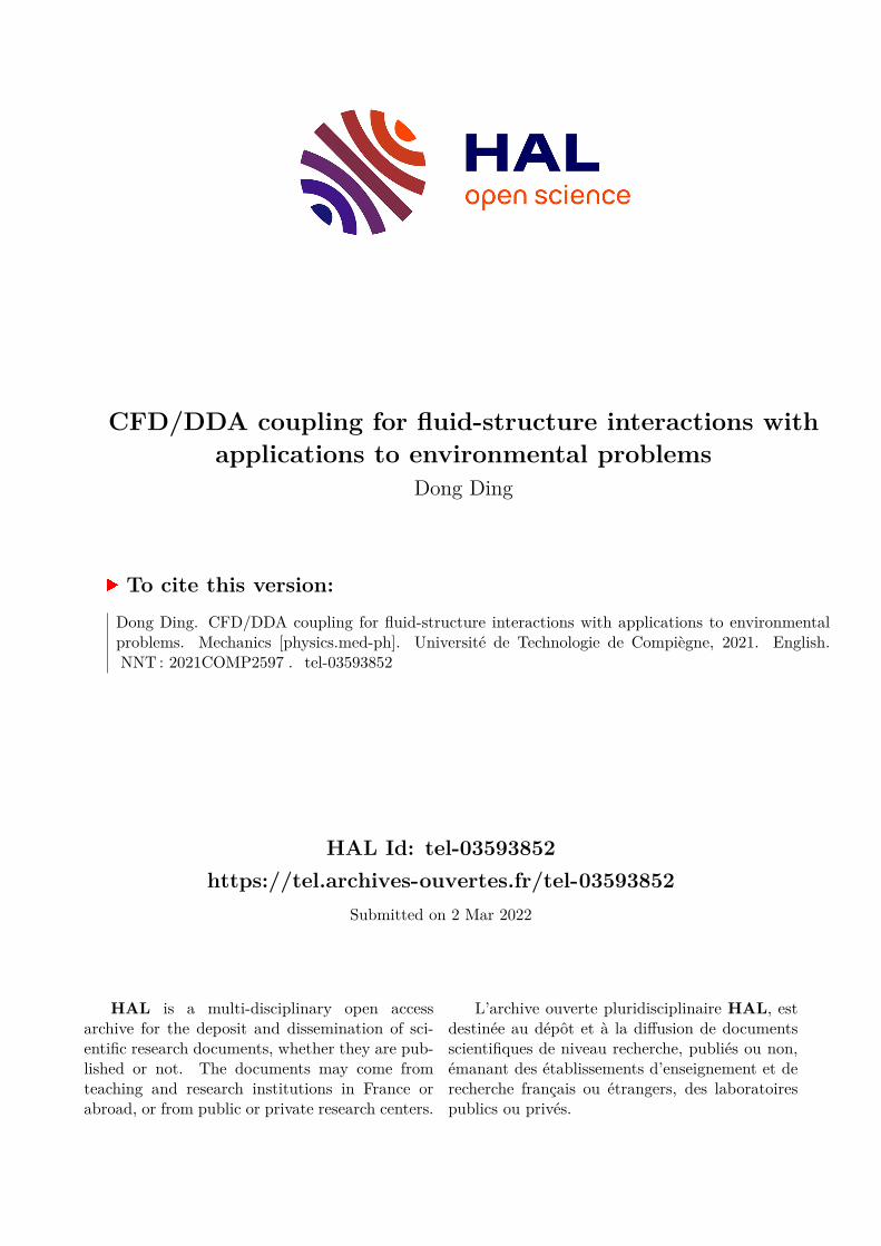
CFD/DDA coupling for fluid-structure interactions with applications to environmental problems
Soutenue le 23 mars 2021 Spécialité : Mécanique Numérique : Unité de recherche en Mécanique - Laboratoire Roberval (FRE UTC - CNRS 2012)
D2597
Dong DING
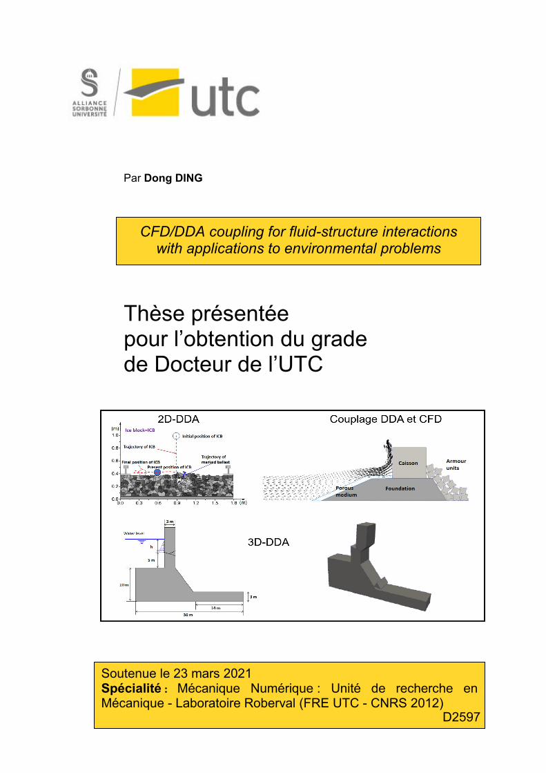
CFD/DDA Coupling for Fluid-structure Interactions with Applications to Environmental Problems
Thèse présentée pour l’obtention du grade de Docteur de l’Université de
Technologie de Compiègne (UTC).
Membres du Jury :S.-S. GUILLOU Professeur des Universités, ESIX Normandie RapporteurH. NACEUR Professeur des Universités, INSA Hauts-de-France RapporteurA. Ibrahimbegovic Professeur des Universités, UTC ExaminateurA. Rassineux Professeur des Universités, UTC ExaminateurE. Hadzalic, Assistant Professeur, University of Sarajevo ExaminateurD. Brancherie Professeur des Universités, UTC InvitéeA. Ouahsine Professeur des Universités, UTC Directeur de thèse
Soutenue le : 23 Mars 2021
Laboratoire Roberval, Unité de Recherche en Mécanique
Spécialité : Mécanique Numérique

CFD/DDA Coupling for Fluid-structureInteractions with Applications to
Environmental Problems
Thesis submitted for the degree of
Doctor at the UT Compiègne-Sorbonne University
by
Dong DINGRoberval Laboratory
UT Compiègne-Sorbonne University
Compiègne, France
23 March 2021


Couplage CFD / DDA pour lesinteractions fluide-structure avec des
applications aux problèmesenvironnementaux
Thèse présentée pour l’obtention
du grade de Docteur
de UT Compiègne-Sorbonne Université
par
Dong DINGLaboratoire Roberval
UT Compiègne-Sorbonne Université
Compiègne, France
23 Mars 2021


I would like to dedicate this thesis to my loving family.

Acknowledgments
This thesis is sponsored by the China Scholarship Council (CSC) and finished inthe Laboratoire Roberval, UT Compiègne-Alliance Sorbonne université under thesupervision of Prof. Abdellatif Ouahsine. I would like to sincerely thank Prof. Ouah-sine for his encourages and helps both in my work and life. His wisdom, knowledgeabove all his high standards stimulated me a lot. I benefited a lot from each con-versation with him and I also learned how to pursue my study and career. He notonly taught me professional knowledge but also a scientific way of thinking andtechnical skills required in research.
I sincerely thank my thesis committee members, Professor Hakim Naceur and Pro-fessor Sylvain S. Guillou for thoroughly reviewing my thesis work, as well as Pro-fessors Adnan Ibrahimbegovic, Alain Rassineux, Delphine Brancherie and Dr. Em-ina Hadzalic for participating in my thesis jury.
I would like to give my sincere gratitude to some people who give me help duringmy PhD study. Dr. Peng Du (Northwestern Polytechnical University) is acknowl-edged for discussing the numerical methods in CFD. Dr. Shengcheng Ji (BeijingAeronautical Science & Technology Research Institute of COMAC) is acknowl-edged for sharing his valuable opinions in simulations. Dr. Weixuan Xiao (Univer-sité Clermont Auvergne) is thanked for cooperating with me to program 3D-DDAcode and sharing some useful C/C++ programming tips in this research. Dr. ErnestoIII Paruli (Université de Technology de Compiègne) is thanked for his friendship,encouragement, especially for his useful paper writing skills. Special thanks go toProf. Guoqing Jing (Beijing Jiaotong University) for his encouragement and guid-ance in high-speed railway engineering.I would like to thank all the colleagues whowork in UTC. They give me lots of help in my french study and life.
Finally, I would like to thank my fiancée Dr. Bei Wu, she not only gave me care andencouragement in life but also gave me many suggestions in my research. I wouldalso thank my parents, who are the strongest support behind me.

Abstract
In numerous applications of environmental fluid mechanics, problems of retroactiveinteraction between the fluid medium and the discrete solid medium are encoun-tered. This requires the implementation of appropriate numerical coupling tech-niques and of discrete element methods to take into account the discrete nature ofthe solid units of the studied medium. This is the case, for example, when studyingthe problems concerning the stability of rockfill dikes or even the flight of high-speed train ballasts, where the solid medium consists of discrete blocks.
In this thesis, the Discontinuous Deformation Analysis (DDA) method is adoptedto study discontinuous and discrete problems. In the first part of the thesis, two-dimensional Discontinuous Deformation Analysis (2-D DDA) is initially used tostudy the ballast flight caused by dropping snow / ice blocks on high-speed rail-ways and to analyze the dynamic behavior of ballast particles during their colli-sion with a snow / ice block. The numerical results show that the velocity, shapeand incident angle of the snow / ice block play an important role in the ballastflight. Specifically, the number and the maximum displacement of ballast particlesincrease with the speed of the train while the incident angle greatly affects the direc-tion of motion of the ballast particles. The shape of the ice block affects the amountand the extent of the ballast flight. Afterward, the coupling between 2D-DDA andthe Computational Fluid Dynamics (CFD) equations (2D-DDA / CFD) is carriedout to study the stability of a breakwater under violent wave impacts by using atriple-coupled Fluid-Porous-Solid model. Here, the fluid model is described by theVolume-Averaged Reynolds-Averaged Navier-Stokes equations in which the non-linear Forchheimer equations for the porous medium are added to the inertia terms.The 2D-DDA method is used to analyze the movement and the stability of the cais-son and armor units by taking into account the shapes of the armor units, as well asthe contact between blocks.
In the second part of the thesis, the 3D version of the DDA method is developedby programming in the C ++ language. Particular attention is given to the detectionof contacts between blocks, considered as rigid solids. Thus, the techniques of theCommon Plane and of the soft contact method are used to avoid the processes ofpenetration between solid blocks. The 3D-DDA method is verified and validatedfirst of all by academic test cases. Then, the 3D-DDA model is tested by a fluid-structure interaction procedure which concerns the stability of a hydraulic gravity

dam with pre-existing cracks. The stability and damage of the structure are exam-ined as the water level rises and as a function of the cohesion between the blocks.
XII


Résumé en Français
Les travaux dans cette thèse concernent le développement de méthodes numériquespour des applications de couplage fluide-structure en mécanique des fluides del’environnement. Il s’agit de mettre en oeuvre des techniques numériques adap-tées au couplage d’un modèle d’éléments discrets (DEM) basé sur la méthoded’Analyse des Déformations Discontinus (DDA), avec un modèle avec maillagebasée sur la méthode d’Eléments finis (FEM). Ces travaux concernent tout d’abord(i) le développement et la mise en place de la version bidimensionnelle (2D), ensuite(ii) le développement de la version 3D de la méthode DDA.
(i) La première partie a nécessité la programmation en langage C++ de la version2D du modèle numérique avec la DDA, ceci en adoptant la méthode de ‘Pénalité’pour la gestion de contacts entre blocs (solides). La validation et l’application decette version 2D du modèle numérique ont été réalisées dans deux cas d’étude:
− le premier cas concerne la Dynamique et l’envol de ballasts par le déplace-ment des trains à Grande Vitesse TGV. L’objectif principal de cette applicationest de déterminer les facteurs d’influence du vol du ballast et d’analyser le com-portement dynamique des particules de ballast lors de leur collision avec un blocneige / glace, ceci en tenant compte de la forme des blocs de glace et les contactsentre les particules de ballast, ainsi que de la vitesse, de la forme et de l’angleincident des blocs neige / glace. Les résultats de ce premier travail ont fait l’objetd’un article publié dans le journal “Transportation Geotechnics”, Elsevier.
− le deuxième cas d’étude, concerne le déplacement d’un caisson induit pardes impacts hydrodynamiques. Un modèle basé sur le couplage de trois milieux(fluide-poreux-solide) est développé. Le milieu fluide est décrit par les équations3D de Navier-Stokes auxquelles sont ajoutées les equations de turbulence à deuxequations (K-epsilon). Le milieu poreux est décrit par les équations non linéairesde Forchheimer, lesquelles sont ajoutées aux termes d’inertie du milieu fluide.Enfin, les movements du milieu solide sont évalués par la méthode d’analyse dedéformation discontinue (DDA), laquelle fait partie des Methods des ElementsDiscrets (DEM). Les résultats de ce deuxième travail ont fait l’objet d’un articlepublié dans le dans journal "Ocean Engineering", Elsevier.
(ii) La deuxième partie, a également nécessité la programmation en langage C++,
porte sur le développement et l’implémentation de la version 3D de la méthodeDDA. Une attention particulière a été portée sur la détection des contacts entreblocs, considérés comme des solides rigides. Ainsi les techniques du Plan Communet de pénalité ont été utilisées pour éviter les processus d’interpénétration entreblocs solides.
Les résultats du modèle 3D-DDA ont été vérifiés et validés tout d’abord par descas tests académiques, sans milieu fluide. Ensuite, le modèle 3D-DDA a été testépar une procédure d’interaction fluide-structure qui concerne la stabilité d’un bar-rage hydraulique présentant des fissures. Dans cette application, il a été examiné lastabilité et l’endommagement de l’ouvrage, au fur et à mesure que le niveau d’eauaugmente et en fonction de la cohésion entre les blocs.
XVI

Contents
Preface I
Acknowledgments IX
Abstract XI
Résumé en Français XV
Contents i
List of figures vii
List of tables xiii
Nomenclature xv
1 Introduction 1
1.1 Motivation and background . . . . . . . . . . . . . . . . . . . . . . 1
1.2 Objective of this thesis . . . . . . . . . . . . . . . . . . . . . . . . 3
1.3 Outline of this thesis . . . . . . . . . . . . . . . . . . . . . . . . . 3
2 State of the art of the DDA method 5
2.1 Introduction . . . . . . . . . . . . . . . . . . . . . . . . . . . . . . 5
2.2 Validations . . . . . . . . . . . . . . . . . . . . . . . . . . . . . . 5
i
2.3 Improvement of DDA . . . . . . . . . . . . . . . . . . . . . . . . . 6
2.3.1 Modification of the DDA Method for rotation error . . . . . 6
2.3.2 High-order displacement function . . . . . . . . . . . . . . 9
2.3.3 Contact mechanics . . . . . . . . . . . . . . . . . . . . . . 10
2.4 Extensions . . . . . . . . . . . . . . . . . . . . . . . . . . . . . . . 13
2.4.1 Circular DDA . . . . . . . . . . . . . . . . . . . . . . . . . 13
2.4.2 Numerical manifold method . . . . . . . . . . . . . . . . . 13
2.4.3 DDA-FEM coupling . . . . . . . . . . . . . . . . . . . . . 15
2.4.4 Fluid-DDA coupling . . . . . . . . . . . . . . . . . . . . . 16
2.5 Applications . . . . . . . . . . . . . . . . . . . . . . . . . . . . . . 19
2.6 Development of 3D-DDA . . . . . . . . . . . . . . . . . . . . . . . 20
2.7 Concluding remarks . . . . . . . . . . . . . . . . . . . . . . . . . . 20
3 Theory of 2D-DDA and CFD/DDA Coupling approach 23
3.1 Introduction . . . . . . . . . . . . . . . . . . . . . . . . . . . . . . 23
3.2 Governing equations of 2D-DDA . . . . . . . . . . . . . . . . . . . 23
3.3 Validations of 2D-DDA . . . . . . . . . . . . . . . . . . . . . . . . 27
3.3.1 Case1: Frictionless impact - Free fall . . . . . . . . . . . . 27
3.3.2 Case 2: Multi-blocks under seismic loading . . . . . . . . . 28
3.4 Governing equations of fluid . . . . . . . . . . . . . . . . . . . . . 30
3.4.1 RANS equations for turbulent flow . . . . . . . . . . . . . 30
3.4.2 Extended Forchheimer equations for porous medium . . . . 30
3.4.3 Volume-averaged RANS equation for incompressible fluid-porous medium coupling . . . . . . . . . . . . . . . . . . . 31
3.4.4 VOF method . . . . . . . . . . . . . . . . . . . . . . . . . 32
ii

3.5 Coupling procedure of Fluid-Solid interaction . . . . . . . . . . . . 33
3.6 Concluding remarks . . . . . . . . . . . . . . . . . . . . . . . . . . 34
4 Mathematical formulation of the 3D-DDA method 35
4.1 Introduction . . . . . . . . . . . . . . . . . . . . . . . . . . . . . . 35
4.2 Displacement function and global equilibrium equations . . . . . . 35
4.2.1 Displacement function . . . . . . . . . . . . . . . . . . . . 35
4.2.2 Global equilibrium equations . . . . . . . . . . . . . . . . . 38
4.3 Governing equations of sub-matrices . . . . . . . . . . . . . . . . . 39
4.3.1 Sub-matrix of elastic strain . . . . . . . . . . . . . . . . . . 39
4.3.2 Sub-matrix of initial stress . . . . . . . . . . . . . . . . . . 42
4.3.3 Sub-matrix of point loading . . . . . . . . . . . . . . . . . 42
4.3.4 Sub-matrix of body force . . . . . . . . . . . . . . . . . . . 43
4.3.5 Sub-matrix of inertia force . . . . . . . . . . . . . . . . . . 44
4.4 Contact between blocks . . . . . . . . . . . . . . . . . . . . . . . . 47
4.4.1 Common-Plane Method . . . . . . . . . . . . . . . . . . . 48
4.4.2 Sub-matrix of normal spring stiffness . . . . . . . . . . . . 53
4.4.3 Sub-matrix of shear spring stiffness . . . . . . . . . . . . . 58
4.4.4 Sub-matrix of friction spring stiffness . . . . . . . . . . . . 61
4.4.5 Open-close iterations . . . . . . . . . . . . . . . . . . . . . 63
4.5 Simplex integration for 3D-DDA . . . . . . . . . . . . . . . . . . . 66
4.6 SOR iteration method . . . . . . . . . . . . . . . . . . . . . . . . . 68
4.7 Procedure for 3D-DDA program . . . . . . . . . . . . . . . . . . . 69
4.8 Concluding remarks . . . . . . . . . . . . . . . . . . . . . . . . . . 71
iii
5 2D-DDA results application to ballast flight in high speed railways 73
5.1 Introduction . . . . . . . . . . . . . . . . . . . . . . . . . . . . . . 73
5.2 Background . . . . . . . . . . . . . . . . . . . . . . . . . . . . . . 73
5.3 Validation: Dynamic behavior of ballast after collision. . . . . . . . 75
5.4 Simulation results . . . . . . . . . . . . . . . . . . . . . . . . . . . 77
5.4.1 Velocity of ice block . . . . . . . . . . . . . . . . . . . . . 77
5.4.2 Incident angle of ice block . . . . . . . . . . . . . . . . . . 82
5.4.3 Shape of ice block . . . . . . . . . . . . . . . . . . . . . . 85
5.5 Concluding remarks . . . . . . . . . . . . . . . . . . . . . . . . . . 89
6 Fluid-Solid coupling application to stability of breakwater 91
6.1 Introduction . . . . . . . . . . . . . . . . . . . . . . . . . . . . . . 91
6.2 Background . . . . . . . . . . . . . . . . . . . . . . . . . . . . . . 91
6.3 Numerical model and validation . . . . . . . . . . . . . . . . . . . 93
6.3.1 Boundary conditions . . . . . . . . . . . . . . . . . . . . . 93
6.3.2 Mesh and time step convergence . . . . . . . . . . . . . . . 94
6.4 Simulation results . . . . . . . . . . . . . . . . . . . . . . . . . . . 95
6.4.1 Flow patterns around the breakwater . . . . . . . . . . . . . 95
6.4.2 Solution behavior with the breakwater seaward slopes . . . 98
6.4.3 Solution behavior with the shape of shoreward armour units 100
6.4.4 Solution behavior with breakwater shoreward slopes . . . . 101
6.4.5 Effect of cohesion . . . . . . . . . . . . . . . . . . . . . . 106
6.5 Concluding remarks . . . . . . . . . . . . . . . . . . . . . . . . . . 109
7 Validations and application for 3D-DDA 111
iv
7.1 Introduction . . . . . . . . . . . . . . . . . . . . . . . . . . . . . . 111
7.2 Validations . . . . . . . . . . . . . . . . . . . . . . . . . . . . . . 111
7.2.1 Case 1: Free fall . . . . . . . . . . . . . . . . . . . . . . . 111
7.2.2 Case 2: Sliding on an inclined plane . . . . . . . . . . . . . 113
7.2.3 Case 3: Multi-blocks under gravity loading . . . . . . . . . 115
7.3 Application: gravity dam failure . . . . . . . . . . . . . . . . . . . 117
7.3.1 Numerical model . . . . . . . . . . . . . . . . . . . . . . . 117
7.3.2 Fluid-structure coupling . . . . . . . . . . . . . . . . . . . 117
7.3.3 Simulation results . . . . . . . . . . . . . . . . . . . . . . 119
7.4 Concluding remarks . . . . . . . . . . . . . . . . . . . . . . . . . . 123
8 Conclusions and future work 125
8.1 Conclusions . . . . . . . . . . . . . . . . . . . . . . . . . . . . . . 125
8.2 Future work . . . . . . . . . . . . . . . . . . . . . . . . . . . . . . 126
Bibliography 127
Appendix A List of publications 145
A.1 Articles . . . . . . . . . . . . . . . . . . . . . . . . . . . . . . . . 145
A.2 Conferences . . . . . . . . . . . . . . . . . . . . . . . . . . . . . . 146
v

List of figures
2.1 Rotation error due to linear displacement function [40] . . . . . . . . 8
2.2 Interaction between two contacting blocks . . . . . . . . . . . . . . . 11
2.3 Rotation and deformation of an ellipse . . . . . . . . . . . . . . . . . 14
2.4 Illustration of an NDDA model [63]. . . . . . . . . . . . . . . . . . . 15
2.5 HYDRO–DDA interface: conversion of fluid pressure into equivalentvertex forces [65] . . . . . . . . . . . . . . . . . . . . . . . . . . . . 17
2.6 DDA and fluid interface: (a) finite element mesh and DDA block;(b) fluid pressures around a DDA block and (c) conversion of fluidpressures into equivalent vertex forces [68]. . . . . . . . . . . . . . . 17
2.7 DDA and SPH interaction [70]. . . . . . . . . . . . . . . . . . . . . 18
2.8 Applications of the DDA method . . . . . . . . . . . . . . . . . . . . 19
2.9 DDA state of the art . . . . . . . . . . . . . . . . . . . . . . . . . . . 21
3.1 The structure of stiffness matrix in the case of three blocks:(a) Loca-tion of three blocks; (b) Structure of stiffness matrix . . . . . . . . . . 26
3.2 Interaction between two contacting blocks . . . . . . . . . . . . . . . 27
3.3 Falling block for testing frictionless impact and elastic rebound: (a)Schematic diagram of free fall motion; (b) Comparison between thetheoretical value (Equation (3.16)) and DDA results for different con-tact stiffness . . . . . . . . . . . . . . . . . . . . . . . . . . . . . . . 28
vii
3.4 Comparison between the experimental results [36] and the numericalresults computed by DEM and DDA. The dimension of one block is48 mm ×48 mm ×29 mm, the mass is 135.5 g, the contact stiff-ness is 107N/m, the friction angle is φ = 34o, and the peak groundaccelerations is 2.15 m/s2 . . . . . . . . . . . . . . . . . . . . . . . 29
3.5 Comparison between the experimental values of ainitiate [36] and DDAresults. . . . . . . . . . . . . . . . . . . . . . . . . . . . . . . . . . . 30
3.6 Fluid/solid interface: (a) fluid finite element mesh and solid; (b) fluidpressures in the mesh points; (c) conversion of fluid pressures intoequivalent vertex forces. . . . . . . . . . . . . . . . . . . . . . . . . 33
4.1 Basic contact types between two 3-D blocks . . . . . . . . . . . . . . 48
4.2 Definition of distances and sign convention of a point to a plane. . . . 49
4.3 Two blocks contacts and the CP: (a) Non-contact, (b) Potential con-tact, (c) Real contact . . . . . . . . . . . . . . . . . . . . . . . . . . 50
4.4 Flowchart of the Common-Plane Method . . . . . . . . . . . . . . . . 52
4.5 Contact between vertex and face, P1 is the penetrate vertex, and P2P3P4
is the entrance face. . . . . . . . . . . . . . . . . . . . . . . . . . . . 53
4.6 Contact types and CP position: (a) Vertex-to-vertex; (b) Vertex-to-edge; (c) Edge-to-edge . . . . . . . . . . . . . . . . . . . . . . . . . 57
4.7 Contact vertex and the entrance face, and the position of shear spring . 59
4.8 Flowchart of open-close iteration . . . . . . . . . . . . . . . . . . . . 65
4.9 Creating oriented simplexes on a face [100]. . . . . . . . . . . . . . . 66
4.10 Flow chart of 3D-DDA procedure. . . . . . . . . . . . . . . . . . . . 70
5.1 Schematic illustration of the mechanism and process of ballast flightcaused by dropping ice block. . . . . . . . . . . . . . . . . . . . . . . 74
5.2 Comparison between the numerical and experimental responses [137]of the blocks for the DDA method. . . . . . . . . . . . . . . . . . . . 76
5.3 Comparison between the numerical and experimental values of N33
[137] for the DDA. . . . . . . . . . . . . . . . . . . . . . . . . . . . 76
viii
5.4 Track bed model . . . . . . . . . . . . . . . . . . . . . . . . . . . . . 77
5.5 Computed ballast flight depending on the initial vertical velocity: (a)Vy= 0 m/s (free fall); (b) Vy = 5 m/s; (c) Vy = 10 m/s . . . . . . . . 79
5.6 Relationship between (a) number of flying ballast particles and initialvertical velocity of ice block, (b) maximum flying height and initialvertical velocity of ice block . . . . . . . . . . . . . . . . . . . . . . 80
5.7 The displacement of (a) ice block and (b) marked ballast for differentinitial vertical velocity in cross section . . . . . . . . . . . . . . . . . 80
5.8 Relationship between ballast flight and longitudinal velocity: (a) Vx= 100 km/h; (b) Vx = 200 km/h; (c) Vx = 300 km/h; (d) Vx = 400km/h . . . . . . . . . . . . . . . . . . . . . . . . . . . . . . . . . . 83
5.9 The displacement of (a) ice block and (b) marked ballast for differentvelocities in longitudinal section . . . . . . . . . . . . . . . . . . . . 84
5.10 Relationship between (a) number of flying ballast particles and ini-tial longitudinal velocity of ice block; (b) maximum flying height andinitial longitudinal velocity of ice block . . . . . . . . . . . . . . . . 84
5.11 Three ice dropping types and incident angles . . . . . . . . . . . . . . 85
5.12 Ballast flight at different incident ejection angles: (a) α = 0o; (b)α = 30o; (c) α = 60o; (d) α = 90o . . . . . . . . . . . . . . . . . . . 86
5.13 The displacement of (a) ice block and (b) marked ballast for differentangles in longitudinal section . . . . . . . . . . . . . . . . . . . . . . 87
5.14 Relationship between ballast flight and ice block shape: (a) Triangle;(b) Circle; (c) Square . . . . . . . . . . . . . . . . . . . . . . . . . . 88
5.15 The displacement of (a) ice block and (b) marked ballast of differentshapes . . . . . . . . . . . . . . . . . . . . . . . . . . . . . . . . . . 89
6.1 Schematic illustration of the computational domain. Wave type: soli-tary wave; wave height hw = 6 m; water depth dw =10 m; armourlayer thickness Ta = 2 m; breakwater caisson height hc =13 m; cais-son position: x/hc = 15.96. The precise location of gauges P1-P5 is2hc, 11hc, 13hc, 14hc and 15.5hc (m), respectively. . . . . . . . . . . 93
ix
6.2 (a) Horizontal velocity and free surface elevation of mesh, and (b)time step convergence at gauge P1 (see Figure 6.1 for the wave pa-rameters and gauges location). . . . . . . . . . . . . . . . . . . . . . 95
6.3 Pattern changes: (a) t = 19.5 s; (b) t = 20.5 s; (c) t = 21.5 s. Theimpacting wave is a solitary wave with a wave height 6 m and a waterheight 10 m. The caisson height is 13 m. The thickness of the porousmedium (porosity = 0.49) is 2 m. The slope is 1:2. . . . . . . . . . . . 96
6.4 Pressure distribution along the vertical caisson. The impacting waveis a solitary wave with a wave height 6 m and a water height 10 m.Point A is located at the bottom of the caisson. Points B-D are 1
3hc,
23hc, and hc away from point A. . . . . . . . . . . . . . . . . . . . . . 97
6.5 Water height evaluation at the vicinity of breakwater (The precise lo-cation of gauges P2-P5 see Figure 6.1) . . . . . . . . . . . . . . . . . 97
6.6 Surface wave deviation with various seaward slopes (1:S). For thewave parameters, see Figure 6.1. The IWHmax of the four slopes are:(a) 1.86 m, (b) 3.71 m, (c) 5.57 m and (d) 9.28 m, respectively. . . . 98
6.7 Variation of IWHmax (see Figure 6.6) for various seaward slopes. . . 99
6.8 Turbulent kinetic energyK for various porous layer thickness in t=24.0s. (see Figure 6.1 for the wave parameters). . . . . . . . . . . . . . . 99
6.9 Shapes of armour units used in the simulation. . . . . . . . . . . . . . 100
6.10 Simulated movement for various shapes of armour units: (a) Cube,(b) Accropod, (c) Tetrapod. The breakwater was subjected to solitarywave impacts whose input external force is calculated by Equation(3.27). (See Figure 6.1 for the wave parameters). . . . . . . . . . . . . 102
6.11 Variation of standard deviations for three shapes of armour units. . . . 103
6.12 Standard deviations for three slopes . . . . . . . . . . . . . . . . . . 104
6.13 Slope of breakwater: (a) slope=√
3:1; (b) slope=1:1; (c) slope=1:2.The shape of armour unit is cube. The breakwater was subjected tosolitary wave impacts whose input external force is calculated byEquation (3.27). (See Figure 6.1 for the wave parameters). . . . . . . 105
x
6.14 Standard deviations for three slopes . . . . . . . . . . . . . . . . . . 106
6.15 Standard deviations for three slopes . . . . . . . . . . . . . . . . . . 107
6.16 Comparison of the motion of cubic units at final position: (a) cohe-sion=0 Pa, tensile strength σt = 0.7 MPa; (b) cohesion= 2 MPa, ten-sile strength σt = 0.7 MPa; (c) Comparison of the effect of cohesion.The breakwater was subjected to solitary wave impacts whose exter-nal force is calculated by Equation (3.27) (See Figure 6.1 for the waveparameters). . . . . . . . . . . . . . . . . . . . . . . . . . . . . . . . 108
6.17 Displacement of cubic armour units 2 and 5 with and without cohesion 109
7.1 Schematic representation of a block in free fall. Falling height h =10.60 m, g = 9.81 m/s2, initial velocity V0 = 0 m/s. . . . . . . . . . 112
7.2 Comparison of analytical and numerical velocities. Falling height h =10.60 m, g = 9.81 m/s2, initial velocity V0 = 0 m/s. . . . . . . . . . 112
7.3 (a) Initial and (b) final positions of sliding model. α = 30o, φ=0. . . . 113
7.4 Time step convergence at the sliding block. Slope angle α = 30o, fric-tion angle φ = 0o, time interval ∆t = 0.1s, 0.01s and 0.001s, respec-tively. Analytical results calculated by the Equation (7.1). . . . . . . . 114
7.5 Variation of the (a) velocity and (b) displacement for different inter-face friction angles. Slope angle α = 30o, friction angle φ= 0o, 10o
and 20o, respectively, time interval ∆t = 0.01 s. Analytical resultscalculated by the Equation (7.1). . . . . . . . . . . . . . . . . . . . . 114
7.6 Variation of the (a) velocity and (b) displacement for different slopeincline angles. Slope angle α= 15o, 30o and 45o, respectively, frictionangle φ= 0o, time interval ∆t = 0.01 s. Analytical results calculatedby the Equation (7.1) . . . . . . . . . . . . . . . . . . . . . . . . . . 115
7.7 Multi-blocks model under gravity loading. ∆t = 0.01 s, time steps = 60.116
7.8 Comparison of 2D and 3D velocity at marked point . . . . . . . . . . 116
7.9 Comparison of 2D and 3D displacement at marked point . . . . . . . 117
7.10 Numerical model of gravity dam with pre-existing cracks . . . . . . . 118
xi

7.11 Fluid-solid interface. . . . . . . . . . . . . . . . . . . . . . . . . . . 119
7.12 Fluid force acting on solid vertex calculated by Equation (7.4). . . . . 120
7.13 Failure behavior of the gravity dam; water height above the cracks h= 4.0 m. . . . . . . . . . . . . . . . . . . . . . . . . . . . . . . . . . 121
7.14 Variation of displacement of block No. 1 for three water levels. . . . . 122
7.15 Variation of displacement of block No. 2 for three water levels. . . . . 122
7.16 Variation of displacement of block No. 1 for different cohesion, waterheight above the cracks h = 4.0 m. . . . . . . . . . . . . . . . . . . . 123
xii
List of tables
2.1 DDA validation by comparing with mathematical analysis . . . . . . 7
2.2 DDA validation by comparing with DEM and tests . . . . . . . . . . 8
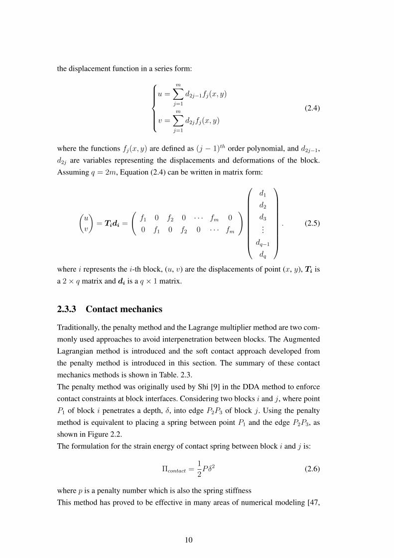
2.3 Summary of contact algorithm . . . . . . . . . . . . . . . . . . . . . 11
4.1 Contact types detected by Common-Plane Method . . . . . . . . . . . 51
4.2 Criteria for contact mode change . . . . . . . . . . . . . . . . . . . . 64
5.1 The material parameters of ice and ballast . . . . . . . . . . . . . . . 77
6.1 Material parameters used for simulations . . . . . . . . . . . . . . . 100
xiii


Nomenclature
List of abbreviations
CFD Computational Fluid DynamicsCP Common-PlaneCPM Common-Plane MethodCRTL Small positive tolerance defined in CPMDDA Discontinuous Deformation AnalysisDEM Distinct Element MethodDIANE Discontinuous, Inhomogeneous, Anisotropic and Non-elasticFDM Finite Difference MethodFEM Finite Element MethodFSI Fluid Structure InteractionFVM Finite Volume MethodIBM Immersed Boundary MethodICB Ice BlockIWH Impacting Wave HeightNMM Numerical Manifold MethodOCS Overhead Contact SystemPIMPLE Merged PISO-SIMPLEPISO Pressure Implicit with Split OperatorRANS Reynolds-Averaged Navier StokesSIMPLE Semi-Implicit Method for Pressure Linked EquationsSOR Successive Over-RelaxationSPH Smoothed Particle HydrodynamicsTKE Turbulence Kinetic EnergyTGV Trains à Grande VitesseUDEC Universal Distinct Element CodeVARANS Volume-Averaged Reynolds-Averaged Navier-StokesVOF Volume-of-Fluid
xv
List of symbols
dn Displacement at normal directiondτ Displacement at shear directiondri Displacement variable of block ifb Body forces applied on a blockg Gravity accelerationh Water height above the crackshw Water depthks, kτ Normal and shear contact stiffnessp, q Two arbitrary orthogonal axes are selected in the CP(x0, y0, z0) Coordinate of Centroid(u0, v0, γ0, εxx, εyy, εxy
)Translations, rotations, normal and shear strains of 2D block
(u, v, w) Displacement of a blockrg Refinement radioCf CohesionCA Added mass termD50 Mean diameter of porous materialD Displacement sub-matricesD,D Acceleration and velocity matricesE Young’s modulusK Stiffness sub-matricesKC Keulegan-Carpenter numberE Elastic matrix of deformation planeF Force sub-matrices(Fx, Fy, Fz) Point loading in x,y,z directionFf Friction forceL, R Strictly lower and upper triangular components of matrixKM Mass per unit volumeMice Mass of ice blockN33 Number of ballast particles thrown higher 330 mmP Penalty spring stiffnessRe Reynolds numberU Fluid velocity〈U〉 Volume-averaged velocityV Total volumeVf Volume of fluid
xvi
Vfall Velocity during the falling processVAmax Vertex on particle A nearest to the CPVBmin Vertex on particle B nearest to the CPTo Period of the oscillation
Greek symbolsα Fluid volume fractionβ1, β2 Coefficients in Newmark methodχ Diagonal component of submatrixKδ Penetration distance between blocksµeff Effective viscosityµt Eddy viscosityν Poisson’s ratio of block materialρ Fluid densityλk Contact force at k-th iterationσ Surface tensionσ0 Initial stress(σx, σy, σz, τyz, τzx, τxy) Stress of blockω Relaxation factor for SOR convergenceΩi Entire volume of block iϕ Friction angle(εx, εy, εz, γyz, γzx, γxy) Strain of blockφ Friction angleΠ Total potential energyΠelastic Elastic strain energyΠinitialstress Initial stress potential energyΠpointload Point loading energyΠbodyforce Body force potential energyΠinertia Inertial energyΠfluid Potential energy contributed due to fluid hydrodynamicsΠcontact Potential energy contributed due to contacts between blocks∆t Time step
xvii

Chapter 1
Introduction
1.1 Motivation and background
During the environmental engineering practice, problems of the discontinuous me-dia are often encountered. For example, the ballast particles in the track and thearmour units in the breakwater, etc. The blocks are largely discontinuous, inhomo-geneous, anisotropic, and non-elastic (DIANE) material [1]. Correctly establishingthe corresponding numerical models based on the real conditions is quite chal-lenging and significant to provide suggestions for the discontinuous environmentalproblems.
Traditionally, several modified continuum approaches are used to investigate thediscontinuous and discrete medium, which can be divided into two types [2]:
− Continuum with joint interface approach;The continuum with the joint interface method introduces the discontinuity in-terface in the form of "joint element" [3] or "discontinuity of displacement" [4]to model the discontinuity.
− Equivalent continuum approach;The equivalent continuum method modifies the constitutive equation of the rockmass to include the mechanical effects of the joints.
These two continuum-based methods have been implemented in Finite Element(FE), Finite Difference (FD) and Boundary Element (BE) methods [5, 6, 7]. Theyhave also been successfully used in applications where no large deformation of therock mass occurs.
The discrete element method based on discontinuous medium mechanics is used tosimulate the motion and collision characteristics of a bulk system. It gives a bettersolution to investigate the large deformation problems. The most commonly used
1
discrete element approaches are Distinct Element Method (DEM) [8] and Discon-tinuous Deformation Analysis (DDA) . The Discontinuous Deformation Analysis(DDA) method was developed by Gen-hua Shi in the late 1980s [9]. Since itspublication, DDA has been verified and applied in numerous studies worldwideand is now considered as a powerful and robust method to address both static anddynamic engineering problems [10]. DDA is somewhat similar to the Finite Ele-ment Method (FEM) for solving stress-displacement problems, but accounts for theinteraction of independent particles (blocks) along discontinuities in fractured andjointed rock masses. DDA is typically formulated as a work-energy method, and canbe derived using the principle of minimum potential energy [9]. Once the equationsof motion are discretized, a step-wise linear time marching scheme in the Newmarkfamily is used for the solution of the equations of motion. The relation betweenadjacent blocks is governed by equations of contact interpenetration and accountsfor friction. DDA adopts a stepwise approach to solve the large displacements thataccompany discontinuous movements between blocks. Since the method accountsfor the inertial forces of the blocks’ mass, it can be used to solve the full dynamicproblem of block motion. The formulation of DDA overcomes the problem of en-ergy dissipation due to algorithmic damping especially when the penalty method isused to handle the contact mechanics between blocks [11, 12] comparing with FEMmethod. Although DDA and DEM are similar in the sense that they both simulatethe behavior of interacting discrete bodies, they are quite different theoretically.While DDA is a displacement method, DEM is a force method. The advantage ofDDA over other rigid body discrete element approaches is DDA gives real dynamicsolution with correct energy consumption and utilizes simple or even higher-orderdeformability of complex shapes [13].
DDA has been widely-used for discontinuous medium simulations. However, theoriginal DDA method still has some limitations which limited its applications. Forexample, it is rarely used to study the problem of a large number of particles;furthermore, it cannot incorporate water pressures in the joints, as well as thereis a gap between two dimensions in reality and no open-source code released for3D-DDA.
2
1.2 Objective of this thesis
This thesis aims to investigate the discontinuous and discrete environmental prob-lems based on the DDA method. The 2D-DDA method will be introduced andthe CFD/DDA coupling approaches will be proposed. Furthermore, the 3D-DDAmethod will be developed and validated. The most important aspects include:
• The literature review of the DDA method will be presented. The validations,modifications, extensions and applications will be introduced in detail.
• The 2D-DDA equations with penalty method will be presented; A couplingstrategy that transmit the pressure of the fluid mesh nodes to the solid polygonvertices will be proposed to achieve fluid-solid coupling.
• The 3D-DDA equations will be developed and programmed. The common-plane method will be used to detect contact; the soft contact method and open-close iteration method will be used to avoid penetration; the Successive Over-Relaxation (SOR) method will be used to solve linear system equations.
• A numerical model based on the 2D-DDA method will be proposed to studythe ballast flight caused by dropping snow / ice blocks in high-speed railways.The dynamic behavior of ballast particles during their collision with a snow / iceblock will be investigated.
• A coupled Fluid-Porous-Solid model will be used to study the stability ofbreakwater. The fluid model will be described by the Volume-Averaged RANSequations. The solid model, which is based on the DDA method, will be used tocompute the movement of the caisson and armour units.
• The 3D-DDA code will be verified by comparing with the analytical results and2D-DDA results. Then a fluid and solid coupling procedure will be proposed tostudy the failure of gravity dam due to the rising water level. The effect of theincreasing water level and cohesion between structures will be studied.
1.3 Outline of this thesis
This thesis is organized as follows:
− Chapter 2 presents the start-of-the-art literature review of the DiscontinuousDeformation Analysis method;
3
− Chapter 3 introduces the brief theory of the 2D-DDA method and the 2D-CFD/DDA coupling approach;
− Chapter 4 is devoted to developing the 3D-DDA program, including thecommon plane method, the open-close iteration method and SOR method.
− Chapter 5 simulates ballast flight caused by dropping snow / ice blocksin high-speed railways. The dynamic behavior of ballast particles during theircollision with a snow / ice block is investigated.
− Chapter 6 carries out the coupled Fluid-Porous-Solid model to study the sta-bility of breakwater. The flow patterns around the breakwater and the movementof the caisson and armour units are simulated.
− Chapter 7 verifies the 3D-DDA by comparing with the analytical resultsand proposes a 3D fluid and solid coupling procedure to study the gravity damfailure.
− Chapter 8 concludes this thesis and gives suggestions for future work.
4
Chapter 2
State of the art of the DDA method
2.1 Introduction
In this chapter, the state-of-the-art review of the DDA method is presented. Thefollowing aspects are emphasized:
• The validations of the DDA method are introduced. The DDA method hasbeen verified by comparing with the mathematical analysis, other computationaltechniques and experimental data;
• The extensions of the DDA method are presented. The DDA method has beencoupled with many numerical methods, for example, FEM, SPH and NMM ect.
• The applications of the DDA method are summarized and the development of3D-DDA method is briefly introduced.
2.2 Validations
The validation works of DDA can be classified into three categories [14]: (1) Com-parison with mathematical analysis; (2) Comparison with other computational tech-niques; and (3) Comparison with experimental data. For the first type, the accuracyof DDA was verified in different aspects, for example, sliding, rotation, tensilestrength, impact, and time integration, as shown in Table 2.1. DDA simulationsshow high acceptable accuracy in most of the common engineering phenomena;however, large body rotation always accumulates the first-order approximation er-ror and causes the block volume expansions; therefore, several modifications havebeen proposed and will be described in Section 2.3.1. For the second type, otherdiscrete numerical technologies were studied to valid the DDA method, as shownin Table 2.2. Dong et al. [15] used a tunnel model to compare the displacementresults between the DDA and FEM predictions. Although the FEM model seemsto predict a larger horizontal displacement component, the displacement patterns
5
caused by the slope excavation predicted by the FEM and DDA models are similar.Furthermore, MacLaughlin et al. [16] compared DDA with another widely usedDEM code: Universal Distinct Element Code (UDEC). The instability and deepfailure of the rock model which has five dip angles combined with three rock massare investigated by DEM and UDEC. 73% of simulations of the two methods areessentially identical. Khan [2] examined the time integration of those two methodsin parallel. UDEC uses an explicit scheme while DDA uses an implicit scheme. Theexplicit scheme has low computational cost while the implicit scheme enhancedstability [17, 18].Validation with respect to experiments are summarized in Table 2.2, where thesliding, shaking and impacting process were investigated. Mcbride et al. [19] es-tablished a joint rock slope model, patterned after Cundall et al. [20]. The DDAsimulation can simulate the failure modes observed experimentally. Ishikawa et al.[21] and Ding et al. [22] studied the dynamic behavior of railroad ballast. Resultsfrom the DDA simulations qualitatively agree with experimental results from triax-ial tests and air cannon impact tests [14].
2.3 Improvement of DDA
Many modifications and improvements to the DDA method have been proposed toovercome some of its limitations and make it more efficient, suitable and practicalon engineering computations.
2.3.1 Modification of the DDA Method for rotation error
Ohnishi et al. [26] and Maclaughlin et al. [40] found large rigid body rotationcauses block expansion. According to the first-order approximation of DDA, thedisplacement of block due to rigid translation and rotation is written as:
u = u0 − (y − y0)r0
v = v0 + (x− x0)r0
(2.1)
while the real displacement should expressed as:
u = u0 + (x− x0)(cosθ − 1)− (y − y0)sinθ
v = v0 + (x− x0)sinθ + (y − y0)(cosθ − 1)(2.2)
6
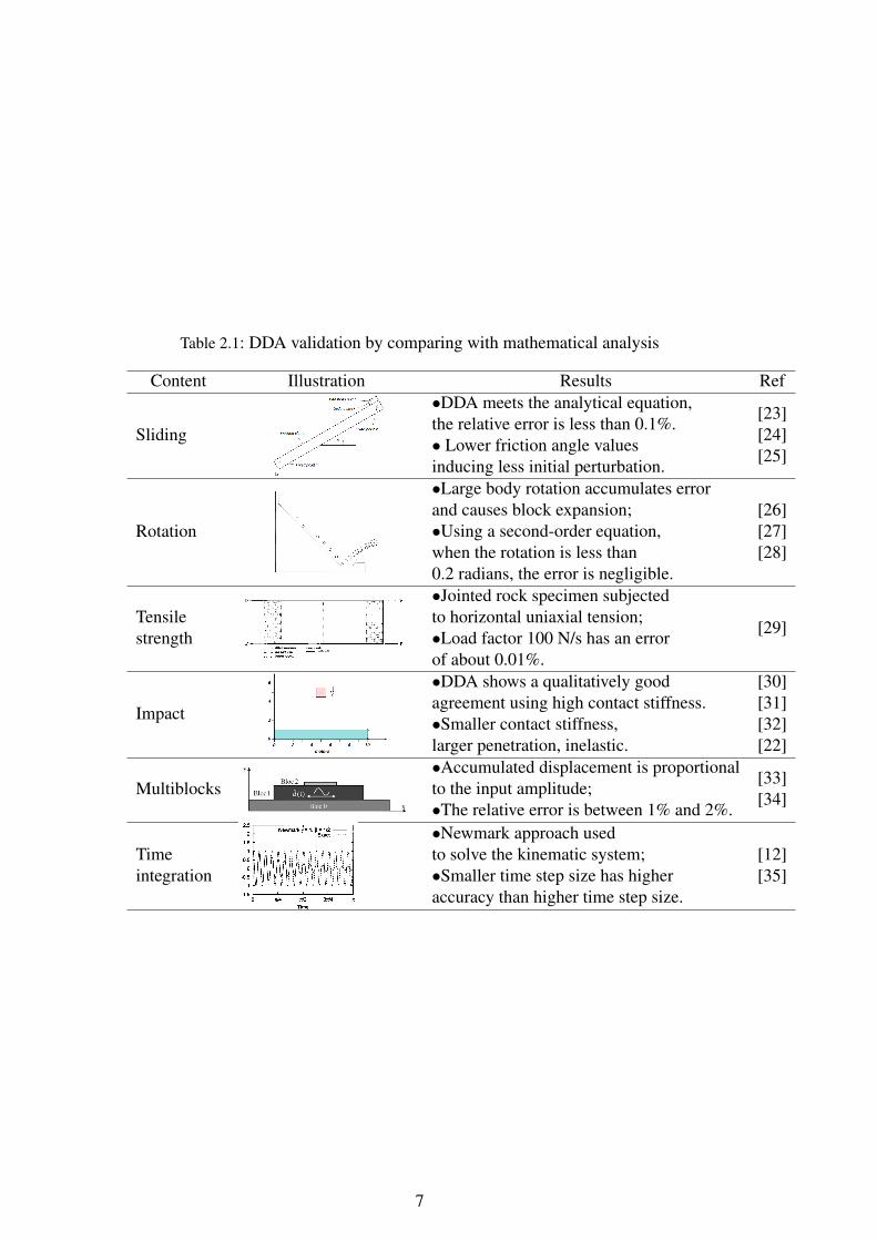
Table 2.1: DDA validation by comparing with mathematical analysis
Content Illustration Results Ref
Sliding
•DDA meets the analytical equation,the relative error is less than 0.1%.• Lower friction angle valuesinducing less initial perturbation.
[23][24][25]
Rotation
•Large body rotation accumulates errorand causes block expansion;•Using a second-order equation,when the rotation is less than0.2 radians, the error is negligible.
[26][27][28]
Tensilestrength
•Jointed rock specimen subjectedto horizontal uniaxial tension;•Load factor 100 N/s has an errorof about 0.01%.
[29]
Impact
•DDA shows a qualitatively goodagreement using high contact stiffness.•Smaller contact stiffness,larger penetration, inelastic.
[30][31][32][22]
Multiblocks•Accumulated displacement is proportionalto the input amplitude;•The relative error is between 1% and 2%.
[33][34]
Timeintegration
•Newmark approach usedto solve the kinematic system;•Smaller time step size has higheraccuracy than higher time step size.
[12][35]
7
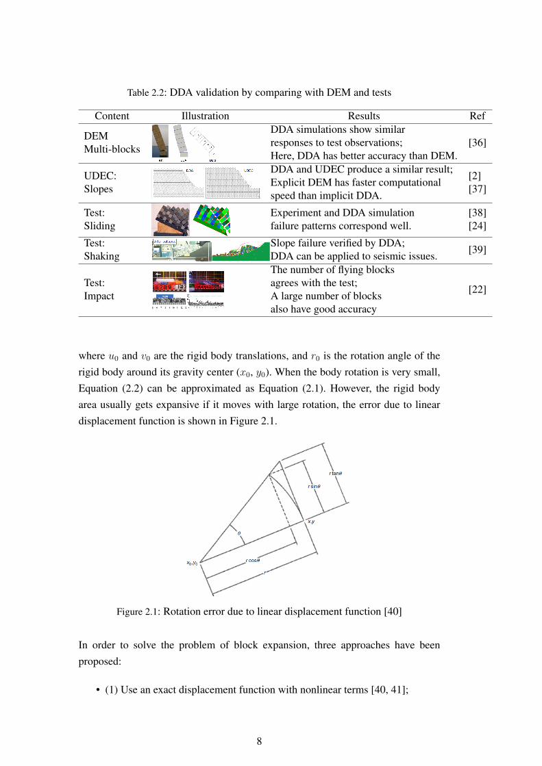
Table 2.2: DDA validation by comparing with DEM and tests
Content Illustration Results Ref
DEMMulti-blocks
DDA simulations show similarresponses to test observations;Here, DDA has better accuracy than DEM.
[36]
UDEC:Slopes
DDA and UDEC produce a similar result;Explicit DEM has faster computationalspeed than implicit DDA.
[2][37]
Test:Sliding
Experiment and DDA simulationfailure patterns correspond well.
[38][24]
Test:Shaking
Slope failure verified by DDA;DDA can be applied to seismic issues. [39]
Test:Impact
The number of flying blocksagrees with the test;A large number of blocksalso have good accuracy
[22]
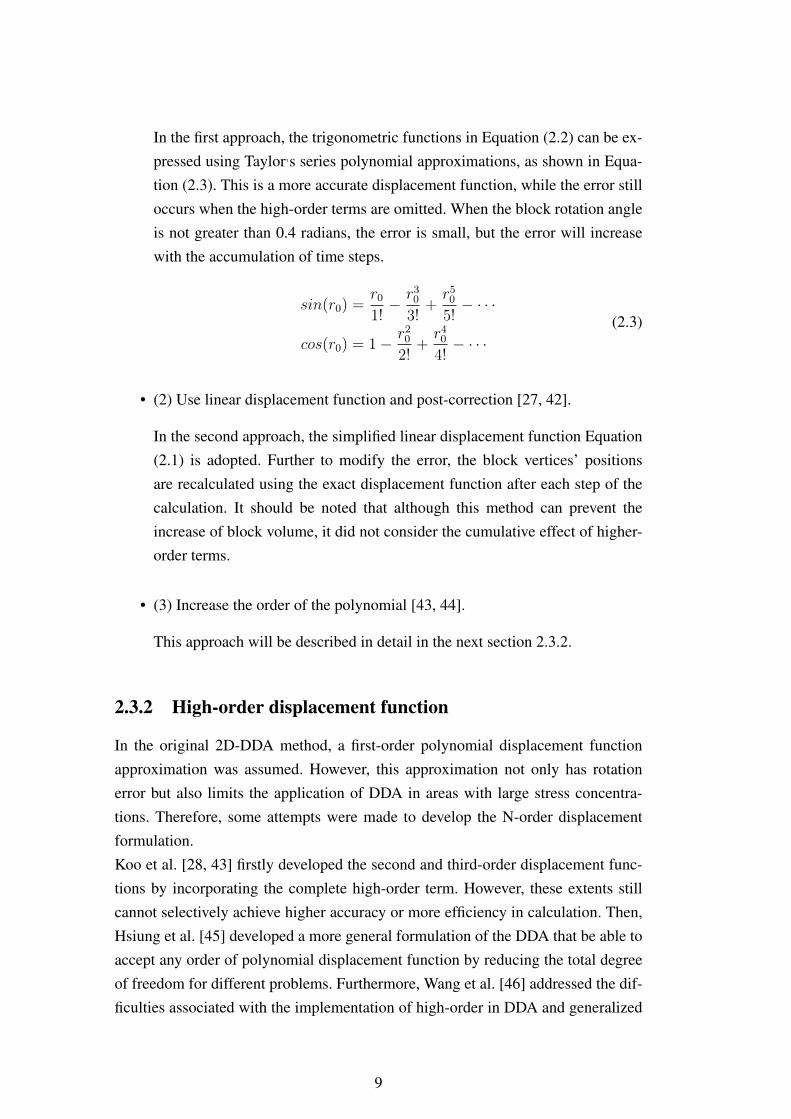
where u0 and v0 are the rigid body translations, and r0 is the rotation angle of therigid body around its gravity center (x0, y0). When the body rotation is very small,Equation (2.2) can be approximated as Equation (2.1). However, the rigid bodyarea usually gets expansive if it moves with large rotation, the error due to lineardisplacement function is shown in Figure 2.1.
Figure 2.1: Rotation error due to linear displacement function [40]
In order to solve the problem of block expansion, three approaches have beenproposed:
• (1) Use an exact displacement function with nonlinear terms [40, 41];
8
In the first approach, the trigonometric functions in Equation (2.2) can be ex-pressed using Taylor,s series polynomial approximations, as shown in Equa-tion (2.3). This is a more accurate displacement function, while the error stilloccurs when the high-order terms are omitted. When the block rotation angleis not greater than 0.4 radians, the error is small, but the error will increasewith the accumulation of time steps.
sin(r0) =r0
1!− r3
0
3!+r5
0
5!− · · ·
cos(r0) = 1− r20
2!+r4
0
4!− · · ·
(2.3)
• (2) Use linear displacement function and post-correction [27, 42].
In the second approach, the simplified linear displacement function Equation(2.1) is adopted. Further to modify the error, the block vertices’ positionsare recalculated using the exact displacement function after each step of thecalculation. It should be noted that although this method can prevent theincrease of block volume, it did not consider the cumulative effect of higher-order terms.
• (3) Increase the order of the polynomial [43, 44].
This approach will be described in detail in the next section 2.3.2.
2.3.2 High-order displacement function
In the original 2D-DDA method, a first-order polynomial displacement functionapproximation was assumed. However, this approximation not only has rotationerror but also limits the application of DDA in areas with large stress concentra-tions. Therefore, some attempts were made to develop the N-order displacementformulation.Koo et al. [28, 43] firstly developed the second and third-order displacement func-tions by incorporating the complete high-order term. However, these extents stillcannot selectively achieve higher accuracy or more efficiency in calculation. Then,Hsiung et al. [45] developed a more general formulation of the DDA that be able toaccept any order of polynomial displacement function by reducing the total degreeof freedom for different problems. Furthermore, Wang et al. [46] addressed the dif-ficulties associated with the implementation of high-order in DDA and generalized
9
the displacement function in a series form:u =
m∑j=1
d2j−1fj(x, y)
v =m∑j=1
d2jfj(x, y)
(2.4)
where the functions fj(x, y) are defined as (j − 1)th order polynomial, and d2j−1,d2j are variables representing the displacements and deformations of the block.Assuming q = 2m, Equation (2.4) can be written in matrix form:
(u
v
)= Tidi =
(f1 0 f2 0 · · · fm 0
0 f1 0 f2 0 · · · fm
)
d1
d2
d3
...dq−1
dq
. (2.5)
where i represents the i-th block, (u, v) are the displacements of point (x, y), Ti isa 2× q matrix and di is a q × 1 matrix.
2.3.3 Contact mechanics
Traditionally, the penalty method and the Lagrange multiplier method are two com-monly used approaches to avoid interpenetration between blocks. The AugmentedLagrangian method is introduced and the soft contact approach developed fromthe penalty method is introduced in this section. The summary of these contactmechanics methods is shown in Table. 2.3.The penalty method was originally used by Shi [9] in the DDA method to enforcecontact constraints at block interfaces. Considering two blocks i and j, where pointP1 of block i penetrates a depth, δ, into edge P2P3 of block j. Using the penaltymethod is equivalent to placing a spring between point P1 and the edge P2P3, asshown in Figure 2.2.The formulation for the strain energy of contact spring between block i and j is:
Πcontact =1
2Pδ2 (2.6)
where p is a penalty number which is also the spring stiffnessThis method has proved to be effective in many areas of numerical modeling [47,
10
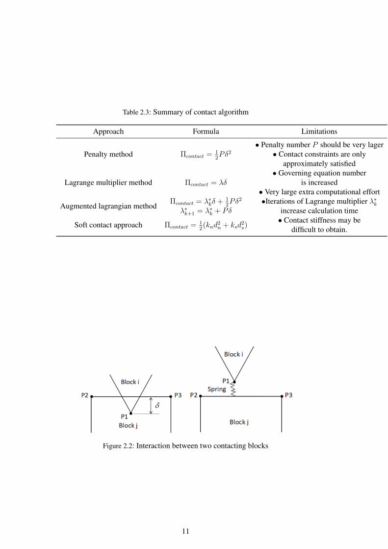
Table 2.3: Summary of contact algorithm
Approach Formula Limitations
Penalty method Πcontact = 12Pδ2
• Penalty number P should be very lager• Contact constraints are only
approximately satisfied
Lagrange multiplier method Πcontact = λδ• Governing equation number
is increased• Very large extra computational effort
Augmented lagrangian methodΠcontact = λ∗kδ + 1
2Pδ2
λ∗k+1 = λ∗k + Pδ•Iterations of Lagrange multiplier λ∗k
increase calculation time
Soft contact approach Πcontact = 12(knd
2n + ksd
2s)
• Contact stiffness may bedifficult to obtain.
Figure 2.2: Interaction between two contacting blocks
11
48]. However, the main limitation with the penalty approach is the choice of thepenalty number, since the solution significantly depends on this number. Further-more, the contact constraints are only approximately satisfied.The Lagrange multiplier method is another one of the most commonly used ap-proaches to solve block contact problems [49, 50, 51]. This method assumes thepenetration δ is caused by an unknown contact force λ, therefore the strain resultingfrom the contact force is defined as:
Πcontact = λδ (2.7)
This method satisfies the contact conditions exactly, whereas the number of gov-erning equations is increased so that extra computational effort is required. TheLagrange approach is rarely used in DDA due to its large consuming computationtime.Combing the above two approaches, Amadei et al. [51] and Lin et al. [52, 53]proposed the augmented Lagrangian formulation to model the contact betweenblocks in the DDA method. The augmented Lagrangian method contains both thepenalty method and the classical Lagrange multiplier method. In this method, aLagrange multiplier λ∗, which represents the contact force, is iteratively calculateduntil the penetration δ below a specified tolerance. The strain energy of contactspring and force is expressed in the following form:
Πcontact = λ∗kδ +1
2Pδ2 (2.8)
where the term λ∗kδ accounts for the work done by the contact forces between theblocks and the term 1
2Pδ2 represents the elastic potential energy associated with the
contact between the blocks. An iterative process is used to calculate the first orderupdated of the Lagrange multiplier, λ∗k, as follows:
λ∗k+1 = λ∗k + Pδ (2.9)
Furthermore, the mechanical model of contacts in other DEM codes also can belearned and used in the DDA method. In the original DDA method, the interpen-etration between blocks is considered non-physical, and with the help of penaltyfunctions, algorithms are used to prevent any intersection of the two contactingbodies [54]. This is a hard contact approach while other DEM codes most use thesoft contact approach in which the interpenetration causes contact forces accordingto the actual contact stiffness, and the arising contact forces are calculated from
12
the depth of the interpenetration [55, 56]. The strain energy due to the normal andtangential contact spring is presented as:
Πcontact =1
2(knd
2n + ksd
2s) (2.10)
where kn and ks are the actual normal and tangential contact stiffness, dn and ds arenormal and tangential penetration distancesThe soft contact approach is a more realistic method but the appropriate propertiesare hard to obtain; the penalty method is simple and easy to add to the program butthe contact constraints meet contact constraints only approximate, and the penaltyspring stiffness has a significant influence on accuracy and convergence. Khan et al.[2] implements the soft contact approach to DDA code that shows good agreementwith analytical results and less residual error.
2.4 Extensions
2.4.1 Circular DDA
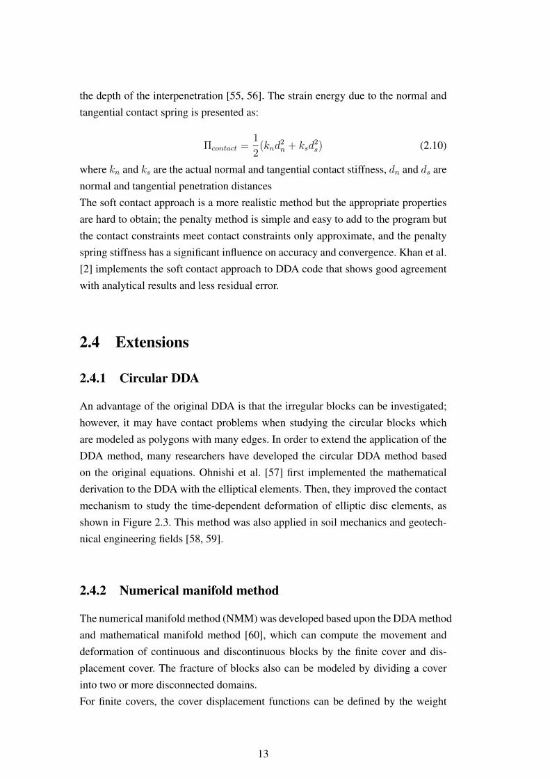
An advantage of the original DDA is that the irregular blocks can be investigated;however, it may have contact problems when studying the circular blocks whichare modeled as polygons with many edges. In order to extend the application of theDDA method, many researchers have developed the circular DDA method basedon the original equations. Ohnishi et al. [57] first implemented the mathematicalderivation to the DDA with the elliptical elements. Then, they improved the contactmechanism to study the time-dependent deformation of elliptic disc elements, asshown in Figure 2.3. This method was also applied in soil mechanics and geotech-nical engineering fields [58, 59].
2.4.2 Numerical manifold method
The numerical manifold method (NMM) was developed based upon the DDA methodand mathematical manifold method [60], which can compute the movement anddeformation of continuous and discontinuous blocks by the finite cover and dis-placement cover. The fracture of blocks also can be modeled by dividing a coverinto two or more disconnected domains.For finite covers, the cover displacement functions can be defined by the weight
13
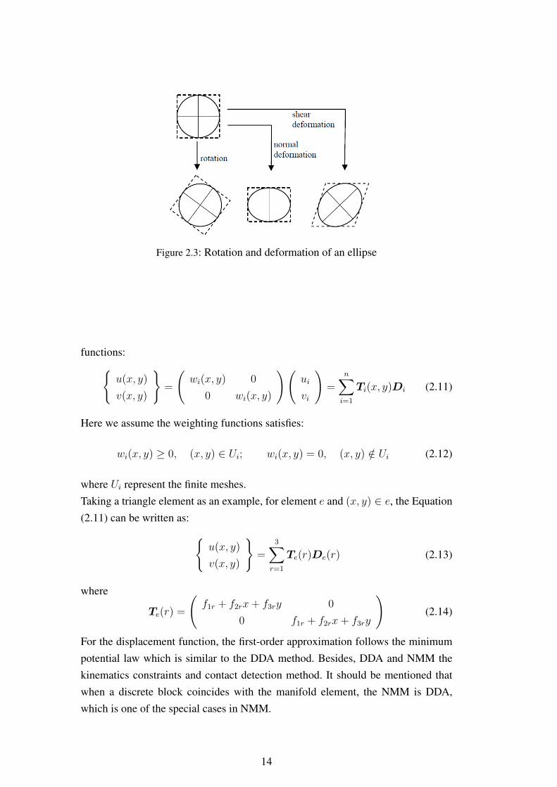
Figure 2.3: Rotation and deformation of an ellipse
functions:u(x, y)
v(x, y)
=
(wi(x, y) 0
0 wi(x, y)
)(ui
vi
)=
n∑i=1
Ti(x, y)Di (2.11)
Here we assume the weighting functions satisfies:
wi(x, y) ≥ 0, (x, y) ∈ Ui; wi(x, y) = 0, (x, y) /∈ Ui (2.12)
where Ui represent the finite meshes.Taking a triangle element as an example, for element e and (x, y) ∈ e, the Equation(2.11) can be written as:
u(x, y)
v(x, y)
=
3∑r=1
Te(r)De(r) (2.13)
where
Te(r) =
(f1r + f2rx+ f3ry 0
0 f1r + f2rx+ f3ry
)(2.14)
For the displacement function, the first-order approximation follows the minimumpotential law which is similar to the DDA method. Besides, DDA and NMM thekinematics constraints and contact detection method. It should be mentioned thatwhen a discrete block coincides with the manifold element, the NMM is DDA,which is one of the special cases in NMM.
14
2.4.3 DDA-FEM coupling
Coupling DDA with the FEM means adding the FEM meshes inside the DDAblocks to get more accurate descriptions of the block’s deformation [61]. The systemequilibrium of FEM and DDA is obtained by the principle of total potential energyminimization.The nodal-based DDA (NDDA) method, which couples the FEM and the DDA, inwhich the DDA kinematics are incorporated with the finite-element mesh, was firstdeveloped by Shyu [62]. Take the triangular elements as an example (see Figure2.4), each element has three nodes (i, j, m) and six displacement variables(ui, vi,uj , vj , um, vm). The displacement (u, v) of any point (x, y) within a triangularelement can be written as:
u
v
=
[Ni 0 Nj 0 Nm 0
0 Ni 0 Nj 0 Nm
]
ui
vi
uj
vj
um
vm
(2.15)
where Ni, Nj and Nm represent the shape functions of the triangular element.
Figure 2.4: Illustration of an NDDA model [63].
Then, Bao et al. [63] extended the NDDA program by employing the Mohr-Coulombfailure criterion to provide a good representation of residual strength conditions toanalyze the fracture. Indeed, by discretizing the block into finite elements, the accu-racy of the DDA method and its ability to resolve stress changes can be improved.Furthermore, the sub-block analysis method [64] can also be used to achieve thesame determination, where each block is divided into smaller sub-blocks, which
15
also can study the fracture by implementing the Mohr-Coulomb failure criterion.
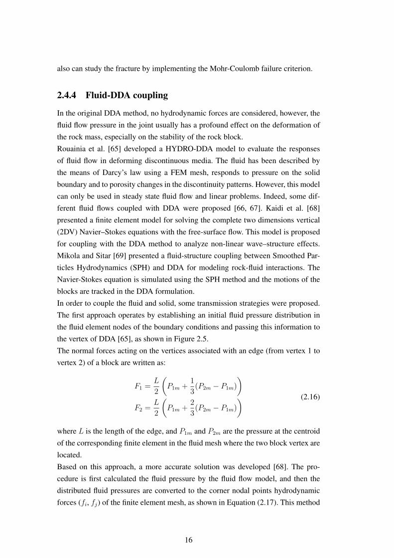
2.4.4 Fluid-DDA coupling
In the original DDA method, no hydrodynamic forces are considered, however, thefluid flow pressure in the joint usually has a profound effect on the deformation ofthe rock mass, especially on the stability of the rock block.Rouainia et al. [65] developed a HYDRO-DDA model to evaluate the responsesof fluid flow in deforming discontinuous media. The fluid has been described bythe means of Darcy’s law using a FEM mesh, responds to pressure on the solidboundary and to porosity changes in the discontinuity patterns. However, this modelcan only be used in steady state fluid flow and linear problems. Indeed, some dif-ferent fluid flows coupled with DDA were proposed [66, 67]. Kaidi et al. [68]presented a finite element model for solving the complete two dimensions vertical(2DV) Navier–Stokes equations with the free-surface flow. This model is proposedfor coupling with the DDA method to analyze non-linear wave–structure effects.Mikola and Sitar [69] presented a fluid-structure coupling between Smoothed Par-ticles Hydrodynamics (SPH) and DDA for modeling rock-fluid interactions. TheNavier-Stokes equation is simulated using the SPH method and the motions of theblocks are tracked in the DDA formulation.In order to couple the fluid and solid, some transmission strategies were proposed.The first approach operates by establishing an initial fluid pressure distribution inthe fluid element nodes of the boundary conditions and passing this information tothe vertex of DDA [65], as shown in Figure 2.5.The normal forces acting on the vertices associated with an edge (from vertex 1 tovertex 2) of a block are written as:
F1 =L
2
(P1m +
1
3(P2m − P1m)
)F2 =
L
2
(P1m +
2
3(P2m − P1m)
) (2.16)
where L is the length of the edge, and P1m and P2m are the pressure at the centroidof the corresponding finite element in the fluid mesh where the two block vertex arelocated.Based on this approach, a more accurate solution was developed [68]. The pro-cedure is first calculated the fluid pressure by the fluid flow model, and then thedistributed fluid pressures are converted to the corner nodal points hydrodynamicforces (fi, fj) of the finite element mesh, as shown in Equation (2.17). This method
16
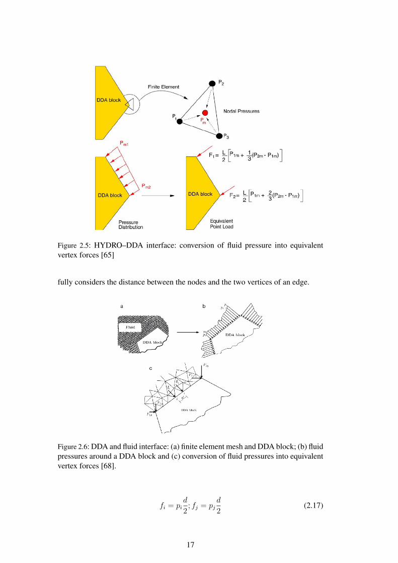
Figure 2.5: HYDRO–DDA interface: conversion of fluid pressure into equivalentvertex forces [65]
fully considers the distance between the nodes and the two vertices of an edge.
Figure 2.6: DDA and fluid interface: (a) finite element mesh and DDA block; (b) fluidpressures around a DDA block and (c) conversion of fluid pressures into equivalentvertex forces [68].
fi = pid
2; fj = pj
d
2(2.17)
17
where pi and pj are the fluid pressure at nodes i and j, and d is the distance of thefinite element edge from node i to node j. Finally, the global forces (F1, F2) actingon the DDA block can be written as:
F1x =n∑i=1
finx(d2
d1 + d2
), F1y =n∑i=1
finy(d2
d1 + d2
)
F2x =n∑i=1
finx(d1
d1 + d2
), F2y =n∑i=1
finy(d1
d1 + d2
)
(2.18)
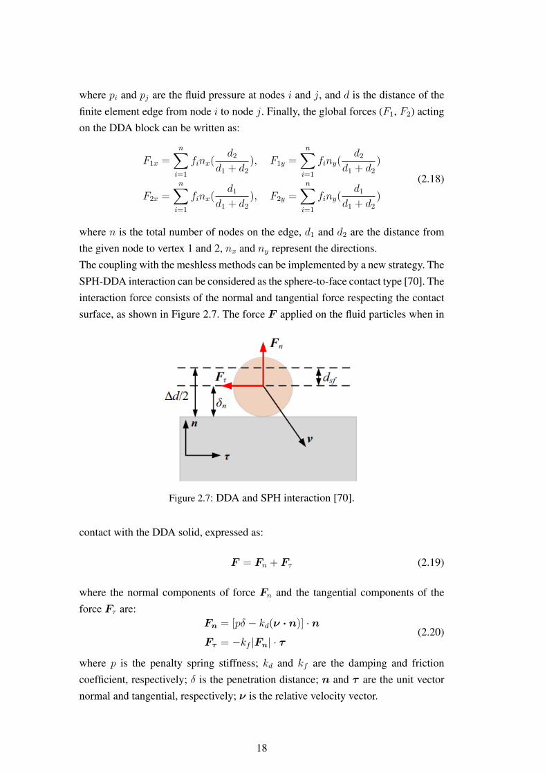
where n is the total number of nodes on the edge, d1 and d2 are the distance fromthe given node to vertex 1 and 2, nx and ny represent the directions.The coupling with the meshless methods can be implemented by a new strategy. TheSPH-DDA interaction can be considered as the sphere-to-face contact type [70]. Theinteraction force consists of the normal and tangential force respecting the contactsurface, as shown in Figure 2.7. The force F applied on the fluid particles when in
Figure 2.7: DDA and SPH interaction [70].
contact with the DDA solid, expressed as:
F = Fn + Fτ (2.19)
where the normal components of force Fn and the tangential components of theforce Fτ are:
Fn = [pδ − kd(ν · n)] · n
Fτ = −kf |Fn| · τ(2.20)
where p is the penalty spring stiffness; kd and kf are the damping and frictioncoefficient, respectively; δ is the penetration distance; n and τ are the unit vectornormal and tangential, respectively; ν is the relative velocity vector.
18

The contact force also applied on the solid block i, which can be treated as a pointloading and added to the force sum-matrices of DDA. The potential energy of thefluid loading is:
Πfluid =− (u, v)
(Fn
Fτ
)
= −DTi T
Ti
(Fn
Fτ
) (2.21)
Then, the derivatives of the potential energy Πfluid is added to the global matrix asan external loading.
2.5 Applications
Due to the unique advantages and continued development of the discontinuous de-formation analysis method, it has been widely applied in geotechnical engineering.It is noted that a number of high-profile projects were analyzed by the DDA method,for example, the three gorges in China[15, 71], Gjovik Olympic Cavern in Norway[72], Pueblo Dam in Colorado[73], King Herod’s Palace [74] and Masada nationalmonument [75] in Israel and so on. Specifically, the original DDA was used for therockfall [76, 77, 78], tunnel [79, 80, 81], and earthquake problems [82, 83, 84]; theextended DDA is widely applied for the blast [85, 86], fracture [87, 63] and waveimpact [68], etc. The applications of the DDA method are shown in Figure 2.8.
Figure 2.8: Applications of the DDA method
19

2.6 Development of 3D-DDA
3D-DDA is currently under extensive research, mainly about its basic theory. G-HShi [88, 89] proposed the basic formulas of 3D-DDA, in which the sub-matricesof point load, initial stress, elastic deformation and inertia forces were provided.Beyabanaki et al. [90] further developed 3D-DDA with higher-order displacementfunctions. Jiao et al. [91, 92] presented a new 3D spherical DDA model. Somecontact algorithms were developed to detect the contact between polygons. Jiangand Yeung [93, 94] developed a vertex-to-face model, Yeung et al. [95] and Wu [96]presented algorithms for edge-to-edge contacts. Liu et al. [97] and Yeung et al. [98,99] introduced the ‘common-plane’ technique to the 3D-DDA method from otherDEM methods. Keneti and Jafari [100] considered the main plane and main contactpoints to identify contact points and types. Beyabanaki and Mikola [101] providea method of using the closest point search algorithm to identify the contact patternbetween two blocks to improve efficiency. Wu et al. [102] proposed an effective androbust spatial contact detection algorithm, which uses a new multi-shell coveringsystem and the decomposition of geometric sub-units, thereby greatly reducing thenumber of contact detection and the number of iterations. The improvement of thecontact judgment algorithm is more and more valued by the majority of scholarsbecause it accounts for nearly 80% of the total computational time. But so far, thereis no efficient, universal, and suitable contact judgment algorithm for a large numberof block analysis calculations in related articles.Similar to 2D-DDA, three-dimensional programs have also been developed andcoupled with other numerical technologies. Grayeli and Hatami [103] coupled theFEM and DDA method using four-noded tetrahedral elements to determine stressesand deformations in practical problems involving fissured elastic media. Wang etal. [104] proposed a coupled DDA–SPH method in three-dimensional case to studythe landslide dams. However, it should be noted that although the theory and somedevelopment of 3D-DDA have been proposed, there is still no open-source or com-mercial solver released, so it is very necessary to develop a 3D program and on thisbasis, in-depth development of three-dimensional applications.
2.7 Concluding remarks
In this chapter, the validations, modifications, extensions and applications of theDDA method were presented and summarized, as shown in Figure 2.9
− For the validations of the DDA method, the sliding, rotation, impact and time
20
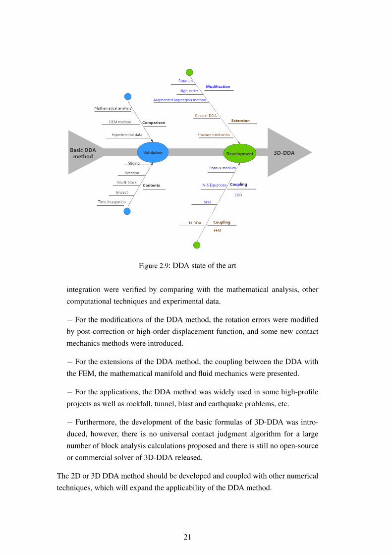
Figure 2.9: DDA state of the art
integration were verified by comparing with the mathematical analysis, othercomputational techniques and experimental data.
− For the modifications of the DDA method, the rotation errors were modifiedby post-correction or high-order displacement function, and some new contactmechanics methods were introduced.
− For the extensions of the DDA method, the coupling between the DDA withthe FEM, the mathematical manifold and fluid mechanics were presented.
− For the applications, the DDA method was widely used in some high-profileprojects as well as rockfall, tunnel, blast and earthquake problems, etc.
− Furthermore, the development of the basic formulas of 3D-DDA was intro-duced, however, there is no universal contact judgment algorithm for a largenumber of block analysis calculations proposed and there is still no open-sourceor commercial solver of 3D-DDA released.
The 2D or 3D DDA method should be developed and coupled with other numericaltechniques, which will expand the applicability of the DDA method.
21

Chapter 3
Theory of 2D-DDA and CFD/DDACoupling approach
3.1 Introduction
In this chapter, the governing equations of the fluid and solid method are introduced.The following aspects are emphasized:
• The 2D-DDA method is introduced briefly. The conditions of the contactsurfaces are enforced through the penalty method in order to avoid the inter-penetration between blocks.
• The fluid flow is described by the RANS equations. The Forchheimer equationsare presented to calculate the flow in the non-linear porous medium.
• The Volume-Averaged Reynolds-Averaged Navier-Stokes (VARANS) equa-tions are proposed, in which the extended Forchheimer law used to calculate theporous medium flow is added to the inertia terms of RANS equations.
• The coupling between the fluid and the solid is carried out by a transmissionstrategy of the fluid mesh nodes’ pressure towards the solid polygon vertices.
3.2 Governing equations of 2D-DDA
In order to investigate the movement and the solid blocks, the Discontinuous De-formation Analysis (DDA) method is used. The DDA method does not have themeshing procedure of blocks and therefore, no refinement is needed to improvethe quality of the calculated solution, which has the advantage of reducing thecomputation time [105, 106]. In the DDA method, the displacement (u, v) at anypoint (x, y) of a block i can be represented by six variables: two translations( u0,
23
v0) of the block gravity center (x0,y0) in x and y directions, a rotation γ0 around(x0,y0), and two normal and a shear strains (εxx, εyy, εxy); therefore, the variablesvector associated with the block i is given:
Di =(u0, v0, γ0, εxx, εyy, εxy
)T(3.1)
According to the first-order expression of any point (x, y), the displacement (u, v)
for an individual block i can be written as:
Ui =
(u
v
)= TiDi (3.2)
where
Ti =
(1 0 −(y − y0) (x− x0) 0 (y − y0)/2
0 1 (x− x0) 0 (y − y0) (x− x0)/2
)(3.3)
The strain of the block i can be expressed by the relationship between the strain anddisplacement:
εi = LUi (3.4)
where L =
∂∂x
0
0 ∂∂y
12∂∂y
12∂∂x
is the differential operator matrix for 2D problem.
Substituting Equation (3.2) into Equation (3.4), we get:
εi = LTiDi = BDi (3.5)
Assuming that the deformation is elastic and linear, the stress tensor is written asfollows:
σi = Eεi = EBDi (3.6)
whereE is the elastic matrix of deformation planes andB =
0 0 0 1 0 0
0 0 0 0 1 0
0 0 0 0 0 1
.
The total potential energy Πp of the block i, defined as the the sum of the elasticstrain energy Πelastic, initial stress potential energy Πinitialstress, body force potentialenergy Πbodyforce, and inertial energy Πinertia, is given by:
24
Πp = Πelastic + Πinitialstress + Πbodyforce + Πinertia
=
∫Ωi
1
2εTi σidΩi +
∫Ωi
εTi σ0dΩi −∫
Ωi
UTi fbdΩi +
∫Ωi
UTi mDidΩi
(3.7)
By using Equation(3.2), it follows:
Πp =
∫Ωi
1
2εTi EεidΩi +
∫Ωi
εTi σ0dΩi −DTi T
Ti
(∫Ωi
fbdΩi −∫
Ωi
TiDidΩi
)(3.8)
where fb denotes the body forces applied on a block i, and M is the block mass perunit area. σ0 is the initial stress of the block.Substituting Equation (3.5) and (3.6) into Equation (3.8), the total potential of asystem of N blocks is expressed as:
Πnp =N∑i=1
(DT
i MDi +1
2DTi KDi −DT
i fe
)(3.9)
where M=∫
ΩiMT Ti TidΩi is the mass matrix, K=
∫ΩiBTEBdΩi is the stiffness
matrix, fe =∫
Ωi(T Ti fb − BTσ0)dΩi is the external forces matrix. According
to the minimized potential energy, the block system equations of motion can berepresented in the compact form:
∂Πnp
∂Di
= 0⇒MD +KD = F (3.10)
Then, the displacement and the velocity in Equation (3.10) can be approximated bythe Newmark−β method:
Dn+1 = Dn + ∆tDn +∆t2
2
[(1− 2β1)Dn + 2β1Dn+1
]Dn+1 = Dn + ∆t
[(1− β2)Dn + β2Dn+1
] (3.11)
where D and D are the acceleration and velocity matrices, respectively, and β1 =
1/2 and β2 = 1 for the implicit scheme ([22]. Substituting Equation (3.11) intoEquation (3.10)), we obtain:
(K +2M
∆t2)Dn+1 = F +
2M
∆tDn (3.12)
25
And then the compact form is given by:
KD = F (3.13)
Consequently, we get the global matrix:
K11 K12 K13 . . . K1n
K21 K22 K23 . . . K2n
K31 K32 K33 . . . K3n
......
......
...Kn1 Kn2 Kn3 . . . Knn
D1
D2
D3
...Dn
=
F1
F2
F3
...Fn
(3.14)
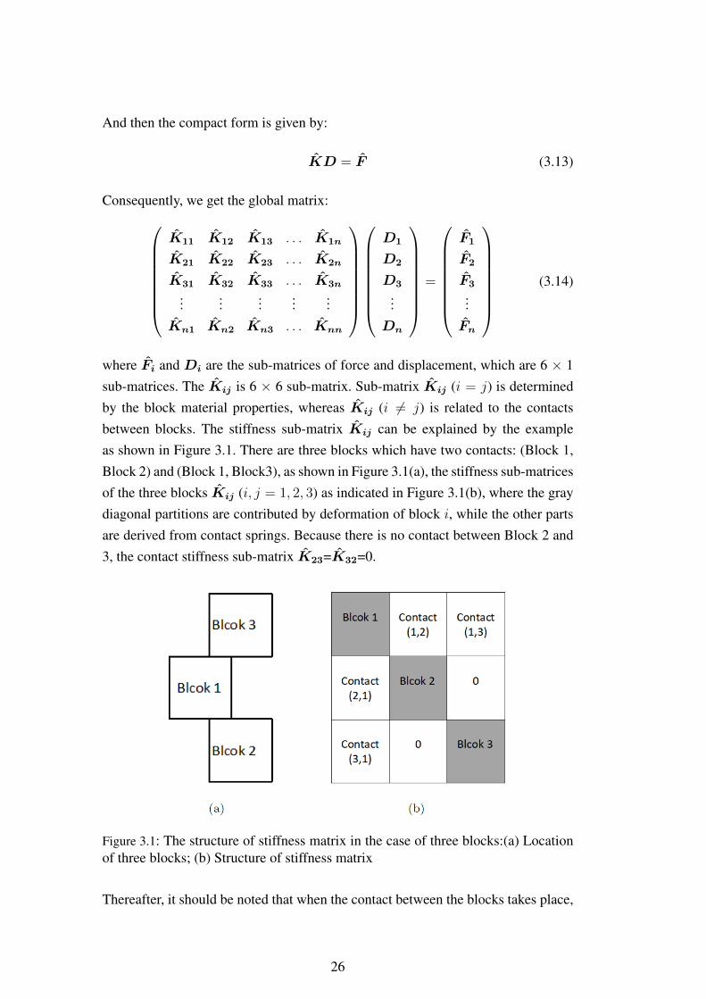
where Fi and Di are the sub-matrices of force and displacement, which are 6 × 1sub-matrices. The Kij is 6 × 6 sub-matrix. Sub-matrix Kij (i = j) is determinedby the block material properties, whereas Kij (i 6= j) is related to the contactsbetween blocks. The stiffness sub-matrix Kij can be explained by the exampleas shown in Figure 3.1. There are three blocks which have two contacts: (Block 1,Block 2) and (Block 1, Block3), as shown in Figure 3.1(a), the stiffness sub-matricesof the three blocks Kij (i, j = 1, 2, 3) as indicated in Figure 3.1(b), where the graydiagonal partitions are contributed by deformation of block i, while the other partsare derived from contact springs. Because there is no contact between Block 2 and3, the contact stiffness sub-matrix K23=K32=0.
Figure 3.1: The structure of stiffness matrix in the case of three blocks:(a) Locationof three blocks; (b) Structure of stiffness matrix
Thereafter, it should be noted that when the contact between the blocks takes place,
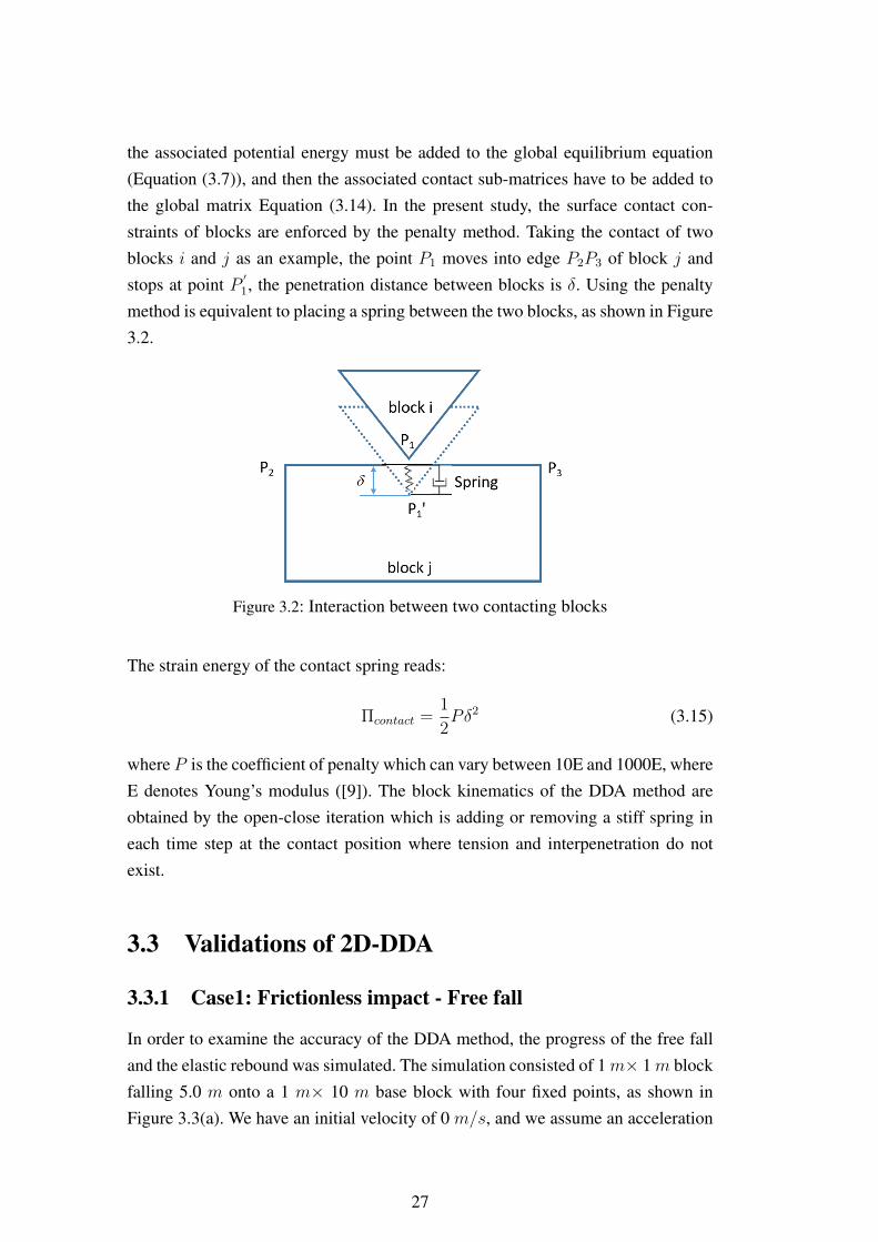
26
the associated potential energy must be added to the global equilibrium equation(Equation (3.7)), and then the associated contact sub-matrices have to be added tothe global matrix Equation (3.14). In the present study, the surface contact con-straints of blocks are enforced by the penalty method. Taking the contact of twoblocks i and j as an example, the point P1 moves into edge P2P3 of block j andstops at point P ′
1, the penetration distance between blocks is δ. Using the penaltymethod is equivalent to placing a spring between the two blocks, as shown in Figure3.2.
Figure 3.2: Interaction between two contacting blocks
The strain energy of the contact spring reads:
Πcontact =1
2Pδ2 (3.15)
where P is the coefficient of penalty which can vary between 10E and 1000E, whereE denotes Young’s modulus ([9]). The block kinematics of the DDA method areobtained by the open-close iteration which is adding or removing a stiff spring ineach time step at the contact position where tension and interpenetration do notexist.
3.3 Validations of 2D-DDA
3.3.1 Case1: Frictionless impact - Free fall
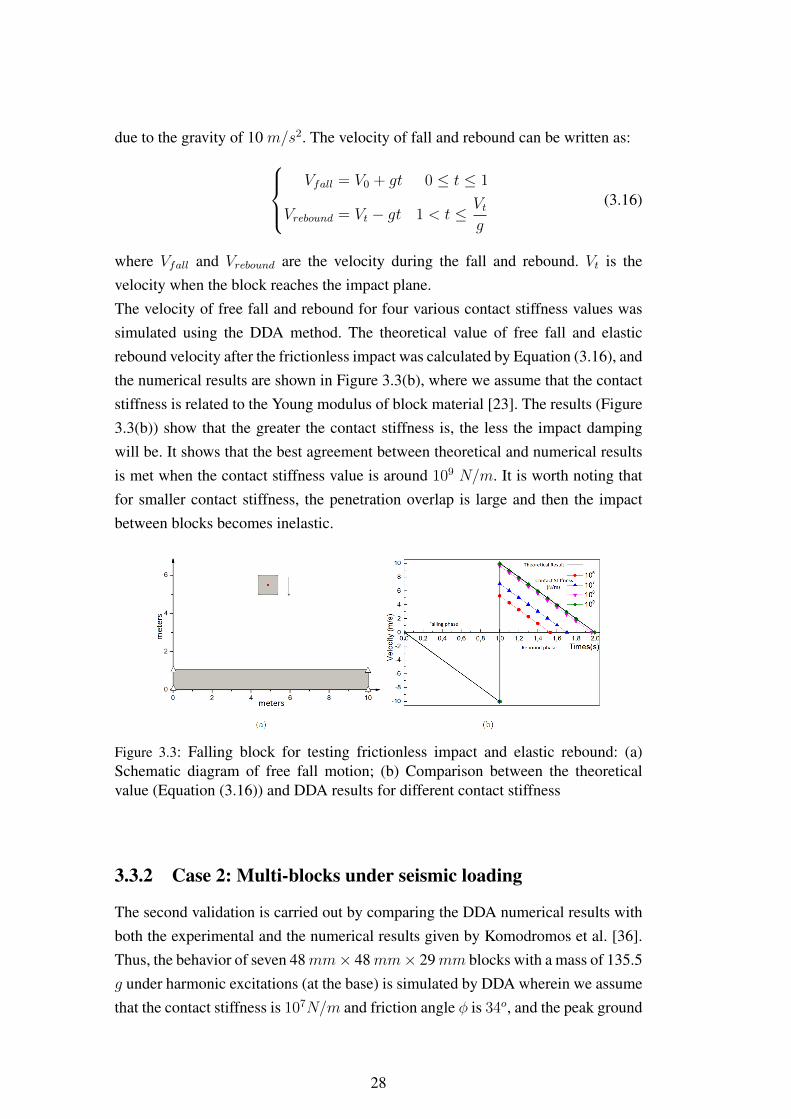
In order to examine the accuracy of the DDA method, the progress of the free falland the elastic rebound was simulated. The simulation consisted of 1m× 1m blockfalling 5.0 m onto a 1 m× 10 m base block with four fixed points, as shown inFigure 3.3(a). We have an initial velocity of 0 m/s, and we assume an acceleration
27
due to the gravity of 10 m/s2. The velocity of fall and rebound can be written as:Vfall = V0 + gt 0 ≤ t ≤ 1
Vrebound = Vt − gt 1 < t ≤ Vtg
(3.16)
where Vfall and Vrebound are the velocity during the fall and rebound. Vt is thevelocity when the block reaches the impact plane.The velocity of free fall and rebound for four various contact stiffness values wassimulated using the DDA method. The theoretical value of free fall and elasticrebound velocity after the frictionless impact was calculated by Equation (3.16), andthe numerical results are shown in Figure 3.3(b), where we assume that the contactstiffness is related to the Young modulus of block material [23]. The results (Figure3.3(b)) show that the greater the contact stiffness is, the less the impact dampingwill be. It shows that the best agreement between theoretical and numerical resultsis met when the contact stiffness value is around 109 N/m. It is worth noting thatfor smaller contact stiffness, the penetration overlap is large and then the impactbetween blocks becomes inelastic.
Figure 3.3: Falling block for testing frictionless impact and elastic rebound: (a)Schematic diagram of free fall motion; (b) Comparison between the theoreticalvalue (Equation (3.16)) and DDA results for different contact stiffness
3.3.2 Case 2: Multi-blocks under seismic loading
The second validation is carried out by comparing the DDA numerical results withboth the experimental and the numerical results given by Komodromos et al. [36].Thus, the behavior of seven 48mm× 48mm× 29mm blocks with a mass of 135.5g under harmonic excitations (at the base) is simulated by DDA wherein we assumethat the contact stiffness is 107N/m and friction angle φ is 34o, and the peak ground
28
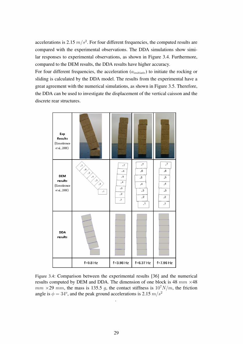
accelerations is 2.15 m/s2. For four different frequencies, the computed results arecompared with the experimental observations. The DDA simulations show simi-lar responses to experimental observations, as shown in Figure 3.4. Furthermore,compared to the DEM results, the DDA results have higher accuracy.For four different frequencies, the acceleration (ainitiate) to initiate the rocking orsliding is calculated by the DDA model. The results from the experimental have agreat agreement with the numerical simulations, as shown in Figure 3.5. Therefore,the DDA can be used to investigate the displacement of the vertical caisson and thediscrete rear structures.
Figure 3.4: Comparison between the experimental results [36] and the numericalresults computed by DEM and DDA. The dimension of one block is 48 mm ×48mm ×29 mm, the mass is 135.5 g, the contact stiffness is 107N/m, the frictionangle is φ = 34o, and the peak ground accelerations is 2.15 m/s2
.
29

Figure 3.5: Comparison between the experimental values of ainitiate [36] and DDAresults.
3.4 Governing equations of fluid
3.4.1 RANS equations for turbulent flow
The fluid flow is described by the Reynolds-Averaged Navier–Stokes (RANS) equa-tions. The mass and momentum conservation functions are [107, 108]:
∂ρ
∂t+∇
(ρU)
= 0 (3.17)
∂(ρU)
∂t+∇
(ρUU
)= −∇P + g X∇ρ+∇
(µeff∇U
)+ σκ∇α (3.18)
where U is the velocity vector, X is the Cartesian position vector, g denotes thegravitational acceleration vector, and ρ represents the weighted averaged density.The term µeff = µ+µt, where µ is the weighted average dynamic viscosity and theµt is the dynamic turbulence viscosity calculated by k − ε model. σκ∇α signifiesthe surface tension effects, where σ is the surface tension, α is the fluid volumefraction, and κ = ∇ α
|α| .
3.4.2 Extended Forchheimer equations for porous medium
Darcy’s law has been traditionally used for describing the transport properties ofporous media; however, as the flow velocity increases, Darcy’s law became in-applicable as the relationship between pressure and velocity becomes non-linear.
30
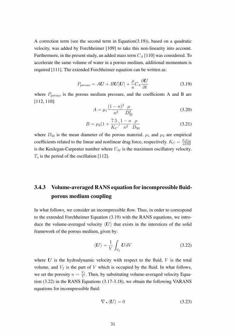
A correction term (see the second term in Equation(3.19)), based on a quadraticvelocity, was added by Forchheimer [109] to take this non-linearity into account.Furthermore, in the present study, an added mass term CA [110] was considered. Toaccelerate the same volume of water in a porous medium, additional momentum isrequired [111]. The extended Forchheimer equation can be written as:
Pporous = AU +BU |U |+ ρ
nCA
∂U
∂t(3.19)
where Pporous is the porous medium pressure, and the coefficients A and B are[112, 110]:
A = µ1(1− n)3
n2
µ
D250
(3.20)
B = µ2(1 +7.5
KC
)1− nn2
ρ
D50
(3.21)
where D50 is the mean diameter of the porous material. µ1 and µ2 are empiricalcoefficients related to the linear and nonlinear drag force, respectively. KC = ToUM
nD50
is the Keulegan-Carpenter number where UM is the maximum oscillatory velocity.To is the period of the oscillation [112].
3.4.3 Volume-averaged RANS equation for incompressible fluid-porous medium coupling
In what follows, we consider an incompressible flow. Thus, in order to correspondto the extended Forchheimer Equation (3.19) with the RANS equations, we intro-duce the volume-averaged velocity 〈U〉 that exists in the interstices of the solidframework of the porous medium, given by:
〈U〉 =1
V
∫Vf
UdV (3.22)
where U is the hydrodynamic velocity with respect to the fluid, V is the totalvolume, and Vf is the part of V which is occupied by the fluid. In what follows,we set the porosity n =
VfV
. Then, by substituting volume-averaged velocity Equa-tion (3.22) in the RANS Equations (3.17-3.18), we obtain the following VARANSequations for incompressible fluid:
∇ 〈U〉 = 0 (3.23)
31
(1 + CA)ρ
n
∂
∂t〈U〉+
ρ
n2〈U〉∇〈U〉 = −∇P + gX ∇ρ+
1
n∇(µeff∇〈U〉
)+ σκ∇α− A〈U〉
n−B| 〈U〉
n|〈U〉n
(3.24)where CA = 0.34 denotes the added mass coefficient, which is kept constant in thepresent study [110].
3.4.4 VOF method
The computational model is built with a two-phase model (Fluid-air) and the freesurface that separates these two phases can cut a cell of the computational mesh intotwo unequal parts. Each part contains a quantity of each phase. In what follows, theVolume-of-Fluid (VOF) method is used to describe the volume fraction of the fluidinside each computational cell which will be transmitted to VARANS. It is basedon the following transport equation [113]:
∂α
∂t+
1
n∇ ·(α〈U〉
)+
1
n∇ ·(α(1− α)〈Uc〉
)= 0 (3.25)
where α is the fluid phase fraction laying between 0 and 1, where α=0 correspondsto full of air and α=1 corresponds to full of fluid. However, in order to obtain physi-cal results, there must be some limitations: a clear interface must be maintained,and α must be limited between 0 and 1. Weller et al. [114] added an artificialcompression term ∇ · α(1 − α). This method only uses non-zero values at theinterface. In addition, |〈Uc〉| = [min(Cα|〈U〉|),max(|〈U〉|)], where the factor Cαcan be specified. If |〈Uc〉| is normal to the interface, the fluid will not be compressed,which points to a larger value of α and therefore from the air to the water phase. Theboundedness of this equation is achieved by the specially designed solver MULES(multi-dimensional universal limiter for explicit solution).In the present study, the VARANS models (see Equations (3.23-3.25)) are solved byusing the PIMPLE algorithm (pressure implicit with the splitting of operators) [115]to compute the pressure and SIMPLE (semi-implicit method for pressure-linkedequations) algorithm to obtain the velocity fields. Its main structure is inherited fromthe original PISO but allows equations to be relaxed to ensure the convergence ofall equations at each time step ([110, 116]).
32
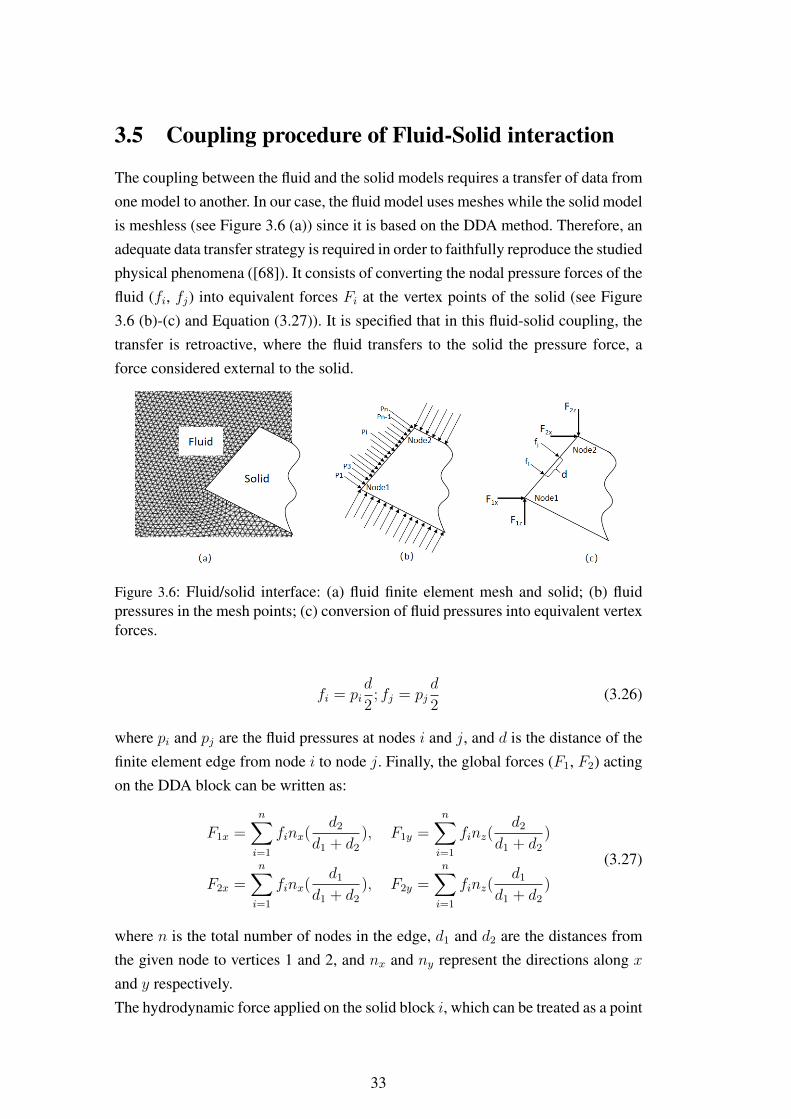
3.5 Coupling procedure of Fluid-Solid interaction
The coupling between the fluid and the solid models requires a transfer of data fromone model to another. In our case, the fluid model uses meshes while the solid modelis meshless (see Figure 3.6 (a)) since it is based on the DDA method. Therefore, anadequate data transfer strategy is required in order to faithfully reproduce the studiedphysical phenomena ([68]). It consists of converting the nodal pressure forces of thefluid (fi, fj) into equivalent forces Fi at the vertex points of the solid (see Figure3.6 (b)-(c) and Equation (3.27)). It is specified that in this fluid-solid coupling, thetransfer is retroactive, where the fluid transfers to the solid the pressure force, aforce considered external to the solid.
Figure 3.6: Fluid/solid interface: (a) fluid finite element mesh and solid; (b) fluidpressures in the mesh points; (c) conversion of fluid pressures into equivalent vertexforces.
fi = pid
2; fj = pj
d
2(3.26)
where pi and pj are the fluid pressures at nodes i and j, and d is the distance of thefinite element edge from node i to node j. Finally, the global forces (F1, F2) actingon the DDA block can be written as:
F1x =n∑i=1
finx(d2
d1 + d2
), F1y =n∑i=1
finz(d2
d1 + d2
)
F2x =n∑i=1
finx(d1
d1 + d2
), F2y =n∑i=1
finz(d1
d1 + d2
)
(3.27)
where n is the total number of nodes in the edge, d1 and d2 are the distances fromthe given node to vertices 1 and 2, and nx and ny represent the directions along xand y respectively.The hydrodynamic force applied on the solid block i, which can be treated as a point
33
loading and added to the force sum-matrices of DDA. The potential energy of thefluid loading is:
Πfluid =− (u, v)
(Fx
Fy
)
= −DTi T
Ti
(Fx
Fy
) (3.28)
The potential energy Πfluid is minimized by taking the derivatives:
fr = −∂Πfluid∂dri
=∂
∂driDT
i TTi
(Fx
Fy
)
= T Ti
(Fx
Fy
)(r = 1, . . . , 6)→ Fi
(3.29)
which is a 6×1 sub-matrix that is added to Fi in the global Equation (3.14).
3.6 Concluding remarks
In this chapter, the governing equations of fluid based on the Volume-AveragedRANS equation and the solid based on the 2D-DDA method were introduced.The 2D-DDA method with the penalty was introduced briefly. The kinematic con-ditions of the contact surfaces were enforced through the penalty method in orderto avoid the inter-penetration between blocks. This method enabled us to take intoaccount the shapes of solid structures, as well as the contact between blocks. Thevalidations of the 2D-DDA method were done by comparing the numerical resultswith the theoretical and the experimental results.The Volume-Averaged Reynolds-Averaged Navier-Stokes (VARANS) equations wereproposed, in which the extended Forchheimer law used to calculate the porousmedium flow was added to the inertia terms of RANS equations.The coupling between the fluid and the solid was carried out by transmitting thepressure of the fluid mesh nodes to the solid polygon vertices. The hydrodynamicforce applied on the solid block, which can be treated as a point loading and addedto the global equilibrium equation.
34
Chapter 4
Mathematical formulation of the3D-DDA method
4.1 Introduction
The two-dimensional approach may only provide a rough approximation of ac-tual behavior. In order to solve the environmental problems accurately, a robustthree-dimensional approach is required. This chapter presents the mathematicalformulations of 3D-DDA and introduces the corresponding program procedure. Thefollowing aspects are emphasized:
• The minimum potential energy method is used in the 3D-DDA method;
• The common-plane method is used to detect the contact between blocks;
• The contact is divided in two types, which are vertex-to-face contact andvertex-to-vertex contact, corresponding normal and shear springs as well as fric-tional forces are added based on the contact type.
• Open-close iteration and soft contact method are used to avoid penetrationsbetween blocks. The SOR method is used to solve linear system equations.
4.2 Displacement function and global equilibrium equa-tions
4.2.1 Displacement function
In this part we will go from standard 2D analysis to 3D Discontinuous DeformationAnalysis (3D-DDA), the following two basic assumptions are still valid:• (1) Each time step satisfies the conditions of very small displacement and defor-mation;
35
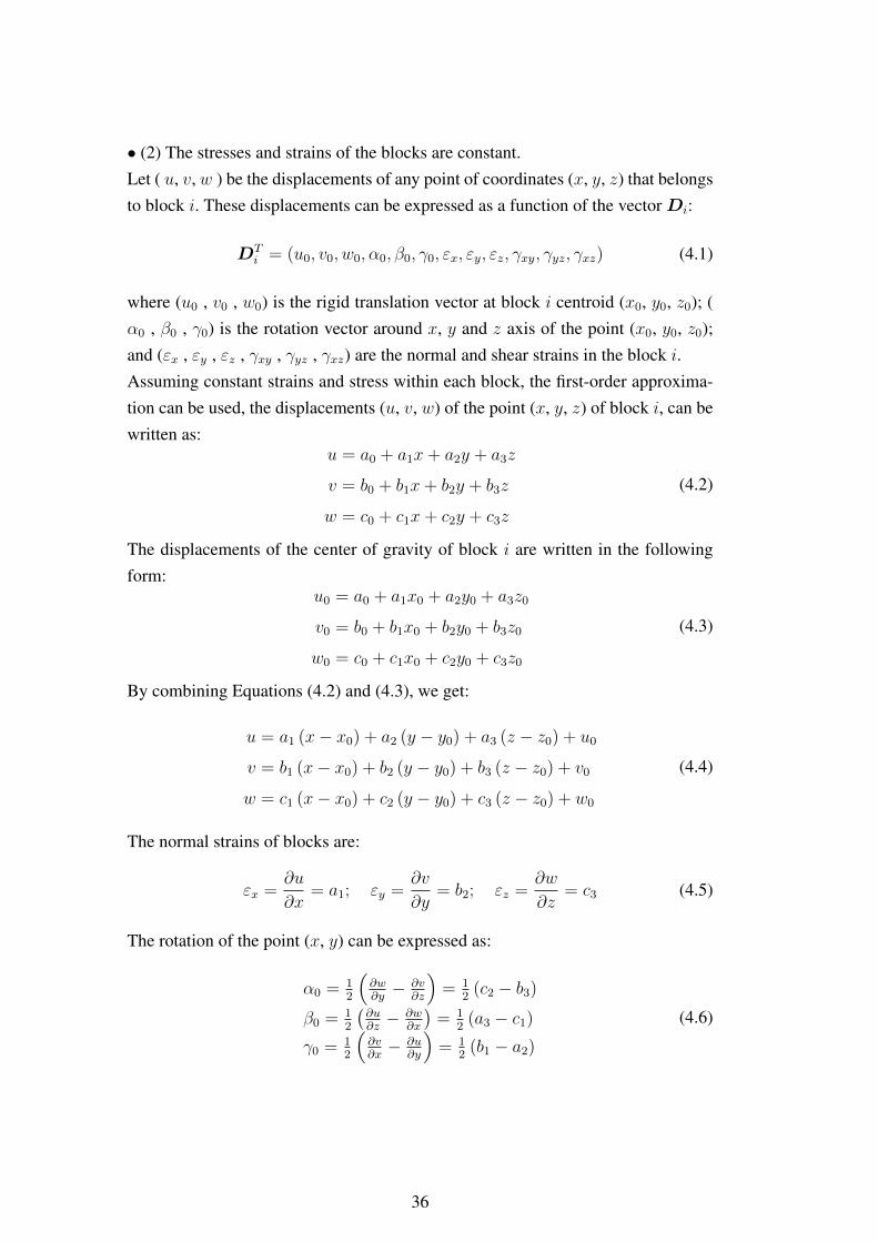
• (2) The stresses and strains of the blocks are constant.Let ( u, v, w ) be the displacements of any point of coordinates (x, y, z) that belongsto block i. These displacements can be expressed as a function of the vectorDi:
DTi = (u0, v0, w0, α0, β0, γ0, εx, εy, εz, γxy, γyz, γxz) (4.1)
where (u0 , v0 , w0) is the rigid translation vector at block i centroid (x0, y0, z0); (α0 , β0 , γ0) is the rotation vector around x, y and z axis of the point (x0, y0, z0);and (εx , εy , εz , γxy , γyz , γxz) are the normal and shear strains in the block i.Assuming constant strains and stress within each block, the first-order approxima-tion can be used, the displacements (u, v, w) of the point (x, y, z) of block i, can bewritten as:
u = a0 + a1x+ a2y + a3z
v = b0 + b1x+ b2y + b3z
w = c0 + c1x+ c2y + c3z
(4.2)
The displacements of the center of gravity of block i are written in the followingform:
u0 = a0 + a1x0 + a2y0 + a3z0
v0 = b0 + b1x0 + b2y0 + b3z0
w0 = c0 + c1x0 + c2y0 + c3z0
(4.3)
By combining Equations (4.2) and (4.3), we get:
u = a1 (x− x0) + a2 (y − y0) + a3 (z − z0) + u0
v = b1 (x− x0) + b2 (y − y0) + b3 (z − z0) + v0
w = c1 (x− x0) + c2 (y − y0) + c3 (z − z0) + w0
(4.4)
The normal strains of blocks are:
εx =∂u
∂x= a1; εy =
∂v
∂y= b2; εz =
∂w
∂z= c3 (4.5)
The rotation of the point (x, y) can be expressed as:
α0 = 12
(∂w∂y− ∂v
∂z
)= 1
2(c2 − b3)
β0 = 12
(∂u∂z− ∂w
∂x
)= 1
2(a3 − c1)
γ0 = 12
(∂v∂x− ∂u
∂y
)= 1
2(b1 − a2)
(4.6)
36
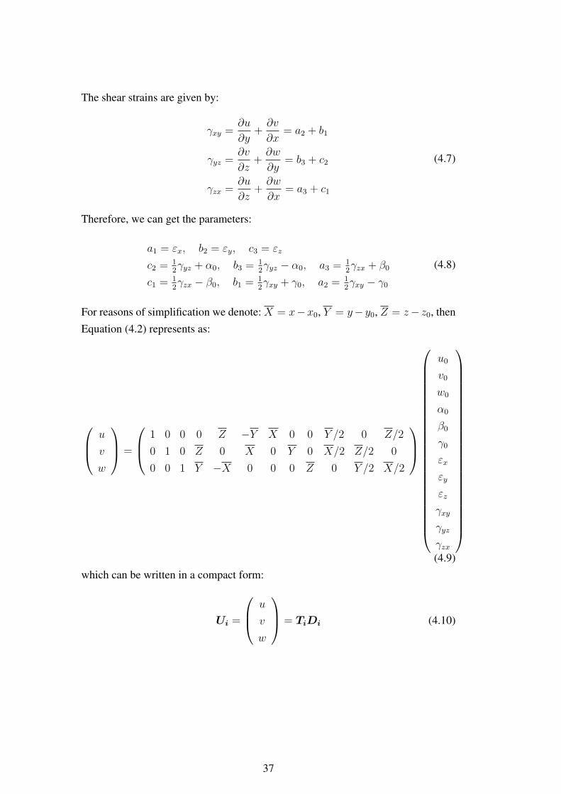
The shear strains are given by:
γxy =∂u
∂y+∂v
∂x= a2 + b1
γyz =∂v
∂z+∂w
∂y= b3 + c2
γzx =∂u
∂z+∂w
∂x= a3 + c1
(4.7)
Therefore, we can get the parameters:
a1 = εx, b2 = εy, c3 = εz
c2 = 12γyz + α0, b3 = 1
2γyz − α0, a3 = 1
2γzx + β0
c1 = 12γzx − β0, b1 = 1
2γxy + γ0, a2 = 1
2γxy − γ0
(4.8)
For reasons of simplification we denote: X = x−x0, Y = y− y0, Z = z− z0, thenEquation (4.2) represents as:
u
v
w
=
1 0 0 0 Z −Y X 0 0 Y /2 0 Z/2
0 1 0 Z 0 X 0 Y 0 X/2 Z/2 0
0 0 1 Y −X 0 0 0 Z 0 Y /2 X/2
u0
v0
w0
α0
β0
γ0
εx
εy
εz
γxy
γyz
γzx
(4.9)
which can be written in a compact form:
Ui =
u
v
w
= TiDi (4.10)
37
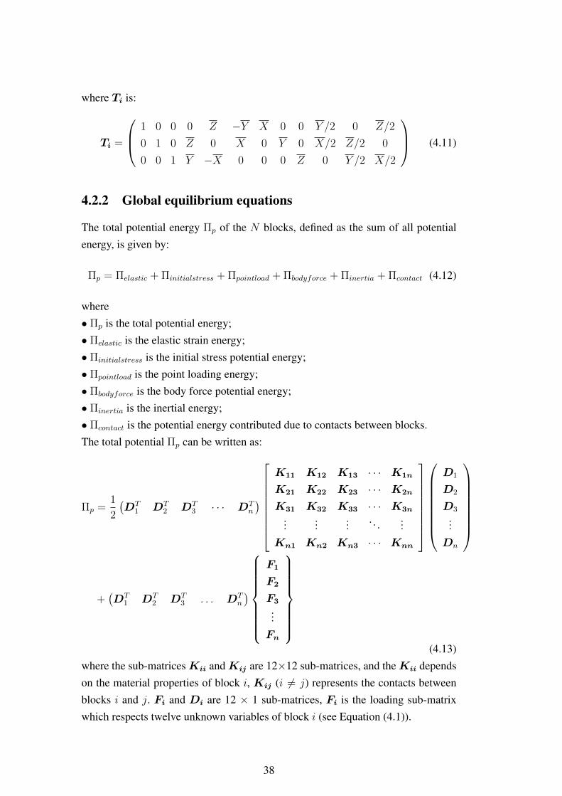
where Ti is:
Ti =
1 0 0 0 Z −Y X 0 0 Y /2 0 Z/2
0 1 0 Z 0 X 0 Y 0 X/2 Z/2 0
0 0 1 Y −X 0 0 0 Z 0 Y /2 X/2
(4.11)
4.2.2 Global equilibrium equations
The total potential energy Πp of the N blocks, defined as the sum of all potentialenergy, is given by:
Πp = Πelastic + Πinitialstress + Πpointload + Πbodyforce + Πinertia + Πcontact (4.12)
where• Πp is the total potential energy;• Πelastic is the elastic strain energy;• Πinitialstress is the initial stress potential energy;• Πpointload is the point loading energy;• Πbodyforce is the body force potential energy;• Πinertia is the inertial energy;• Πcontact is the potential energy contributed due to contacts between blocks.The total potential Πp can be written as:
Πp =1
2
(DT
1 DT2 DT
3 · · · DTn
)
K11 K12 K13 · · · K1n
K21 K22 K23 · · · K2n
K31 K32 K33 · · · K3n
......
... . . . ...Kn1 Kn2 Kn3 · · · Knn
D1
D2
D3
...Dn
+(DT
1 DT2 DT
3 . . . DTn
)
F1
F2
F3
...Fn
(4.13)
where the sub-matricesKii andKij are 12×12 sub-matrices, and theKii dependson the material properties of block i, Kij (i 6= j) represents the contacts betweenblocks i and j. Fi and Di are 12 × 1 sub-matrices, Fi is the loading sub-matrixwhich respects twelve unknown variables of block i (see Equation (4.1)).
38
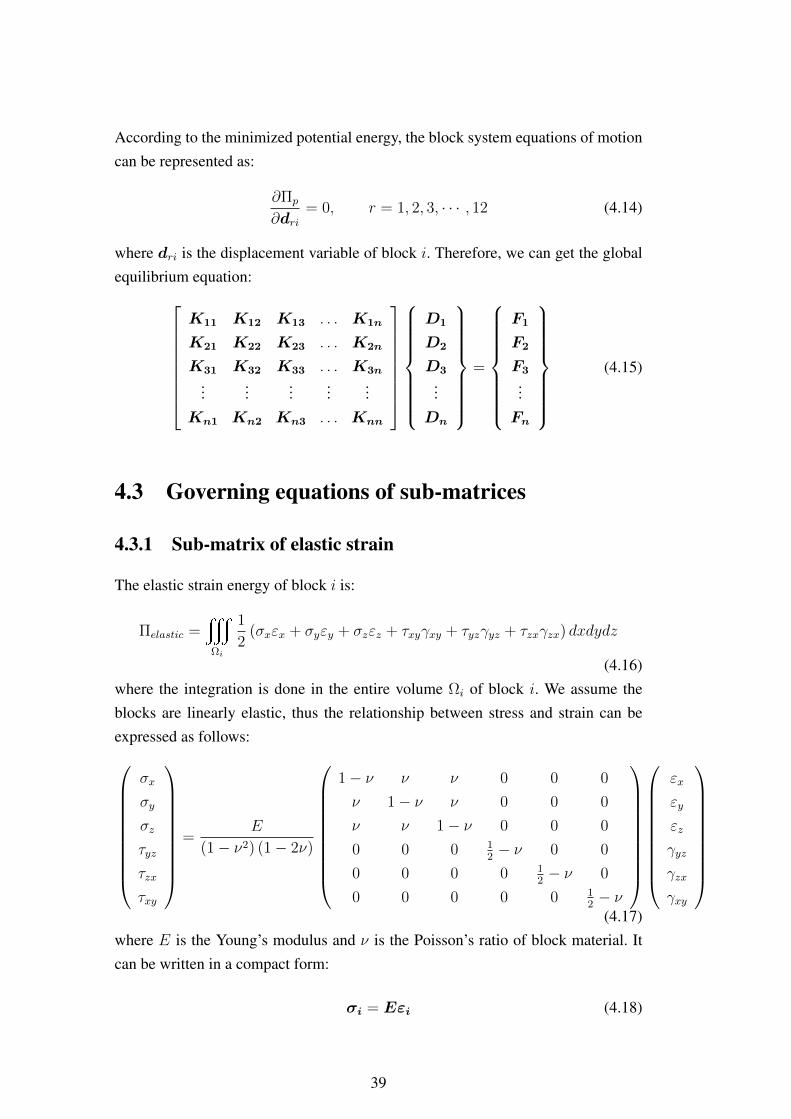
According to the minimized potential energy, the block system equations of motioncan be represented as:
∂Πp
∂dri= 0, r = 1, 2, 3, · · · , 12 (4.14)
where dri is the displacement variable of block i. Therefore, we can get the globalequilibrium equation:
K11 K12 K13 . . . K1n
K21 K22 K23 . . . K2n
K31 K32 K33 . . . K3n
......
......
...Kn1 Kn2 Kn3 . . . Knn
D1
D2
D3
...Dn
=
F1
F2
F3
...Fn
(4.15)
4.3 Governing equations of sub-matrices
4.3.1 Sub-matrix of elastic strain
The elastic strain energy of block i is:
Πelastic =y
Ωi
1
2(σxεx + σyεy + σzεz + τxyγxy + τyzγyz + τzxγzx) dxdydz
(4.16)where the integration is done in the entire volume Ωi of block i. We assume theblocks are linearly elastic, thus the relationship between stress and strain can beexpressed as follows:
σx
σy
σz
τyz
τzx
τxy
=
E
(1− ν2) (1− 2ν)
1− ν ν ν 0 0 0
ν 1− ν ν 0 0 0
ν ν 1− ν 0 0 0
0 0 0 12− ν 0 0
0 0 0 0 12− ν 0
0 0 0 0 0 12− ν
εx
εy
εz
γyz
γzx
γxy
(4.17)
where E is the Young’s modulus and ν is the Poisson’s ratio of block material. Itcan be written in a compact form:
σi = Eεi (4.18)
39
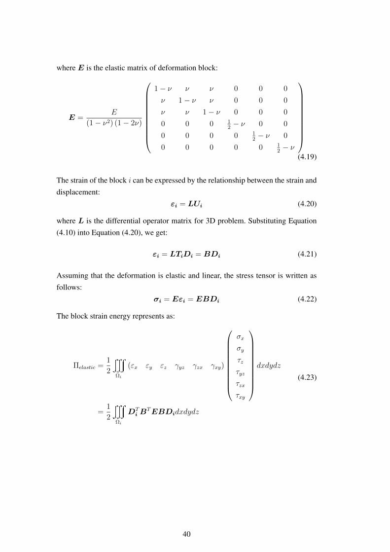
where E is the elastic matrix of deformation block:
E =E
(1− ν2) (1− 2ν)
1− ν ν ν 0 0 0
ν 1− ν ν 0 0 0
ν ν 1− ν 0 0 0
0 0 0 12− ν 0 0
0 0 0 0 12− ν 0
0 0 0 0 0 12− ν
(4.19)
The strain of the block i can be expressed by the relationship between the strain anddisplacement:
εi = LUi (4.20)
where L is the differential operator matrix for 3D problem. Substituting Equation(4.10) into Equation (4.20), we get:
εi = LTiDi = BDi (4.21)
Assuming that the deformation is elastic and linear, the stress tensor is written asfollows:
σi = Eεi = EBDi (4.22)
The block strain energy represents as:
Πelastic =1
2
y
Ωi
(εx εy εz γyz γzx γxy)
σx
σy
τz
τyz
τzx
τxy
dxdydz
=1
2
y
Ωi
DTi B
TEBDidxdydz
(4.23)
40

where the Ei = BTEB is a 12× 12 matrix:
Ei =E
(1− ν2) (1− 2ν)
0 0 0 0 0 0 0 0 0 0 0 0
0 0 0 0 0 0 0 0 0 0 0 0
0 0 0 0 0 0 0 0 0 0 0 0
0 0 0 0 0 0 0 0 0 0 0 0
0 0 0 0 0 0 0 0 0 0 0 0
0 0 0 0 0 0 0 0 0 0 0 0
0 0 0 0 0 0 1− ν ν ν 0 0 0
0 0 0 0 0 0 ν 1− ν ν 0 0 0
0 0 0 0 0 0 ν ν 1− ν 0 0 0
0 0 0 0 0 0 0 0 0 12− ν 0 0
0 0 0 0 0 0 0 0 0 0 12− ν 0
0 0 0 0 0 0 0 0 0 0 0 12− ν
(4.24)
Therefore, the block strain energy can be written as:
Πelastic =1
2
y
Ωi
DTi EiDidxdydz
=Vi2DTi EiDi
(4.25)
where Vi is the volume of block i. Based on the minimization of the strain energyΠelastic, we have:
Krs =∂2Πe
∂dri∂dsi
=Vi2
∂2
∂dridsi
(DTi EiDi
)= ViEi r, s = 1, 2, 3 · · · , 12→Kii
(4.26)
which is added to the sub-matrixKii in the global Equation (4.15).
41
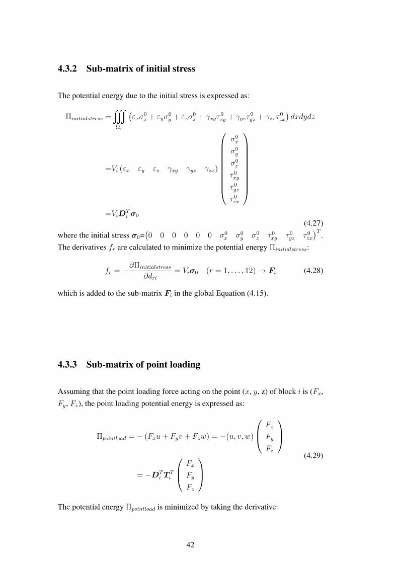
4.3.2 Sub-matrix of initial stress
The potential energy due to the initial stress is expressed as:
Πinitialstress =y
Ωi
(εxσ
0x + εyσ
0y + εzσ
0z + γxyτ
0xy + γyzτ
0yz + γzxτ
0zx
)dxdydz
=Vi (εx εy εz γxy γyz γzx)
σ0x
σ0y
σ0z
τ 0xy
τ 0yz
τ 0zx
=ViD
Ti σ0
(4.27)where the initial stress σ0=
(0 0 0 0 0 0 σ0
x σ0y σ0
z τ 0xy τ 0
yz τ 0zx
)T .The derivatives fr are calculated to minimize the potential energy Πinitialstress:
fr = −∂Πinitialstress
∂dri= Viσ0 (r = 1, . . . , 12)→ Fi (4.28)
which is added to the sub-matrix Fi in the global Equation (4.15).
4.3.3 Sub-matrix of point loading
Assuming that the point loading force acting on the point (x, y, z) of block i is (Fx,Fy, Fz), the point loading potential energy is expressed as:
Πpointload =− (Fxu+ Fyv + Fzw) = −(u, v, w)
Fx
Fy
Fz
= −DTi T
Ti
Fx
Fy
Fz
(4.29)
The potential energy Πpointload is minimized by taking the derivative:
42

fr = −∂Πpointload
∂dri=
∂
∂driDT
i TTi
Fx
Fy
Fz
= T Ti
Fx
Fy
Fz
(r = 1, . . . , 12)→ Fi
(4.30)
which is a 12×1 sub-matrix that is added to Fi in the global Equation (4.15).
4.3.4 Sub-matrix of body force
Assuming that the body force (fx, fy, fz) is the constant volume load acting onblock i, then the potential energy is:
Πbodyforce =−y
Ωi
(u v w)
fx
fy
fz
dxdydz
=−DTi
(yΩi
T Ti dxdydz
) fx
fy
fz
(4.31)
The coordinates of centre of gravity of block i are (x0, y0, z0) which can be ex-pressed as:
x0 =SxVi, y0 =
SyVi, z0 =
SzVi
(4.32)
where Sx =t
Ωixdxdydz, Sy =
tΩiydxdydz, Sz =
tΩizdxdydz and Vi =t
Ωidxdydz. Vi is the volume of block i.
43
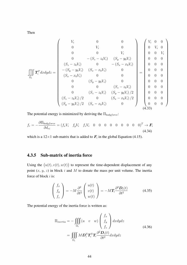
Then
y
Ωi
T Ti dxdydz =
Vi 0 0
0 Vi 0
0 0 Vi
0 − (Sz − z0Vi) (Sy − y0Vi)
(Sz − z0Vi) 0 − (Sx − x0Vi)
− (Sy − y0Vi) (Sx − x0Vi) 0
(Sx − x0Vi) 0 0
0 (Sy − y0Vi) 0
0 0 (Sz − z0Vi)
0 (Sz − z0Vi) (Sy − y0Vi) /2
(Sz − z0Vi) /2 0 (Sx − x0Vi) /2
(Sy − y0Vi) /2 (Sx − x0Vi) 0
=
Vi 0 0
0 Vi 0
0 0 Vi
0 0 0
0 0 0
0 0 0
0 0 0
0 0 0
0 0 0
0 0 0
0 0 0
0 0 0
(4.33)
The potential energy is minimized by deriving the Πbodyforce:
fr = −∂Πbodyforce
∂dri= (fxVi fyVi fzVi 0 0 0 0 0 0 0 0 0)T → Fi
(4.34)which is a 12×1 sub-matrix that is added to Fi in the global Equation (4.15).
4.3.5 Sub-matrix of inertia force
Using the(u(t), v(t), w(t)
)to represent the time-dependent displacement of any
point (x, y, z) in block i and M to donate the mass per unit volume. The inertiaforce of block i is: fx
fy
fz
= −M ∂2
∂t2
u(t)
v(t)
w(t)
= −MTi∂2Di(t)
∂t2(4.35)
The potential energy of the inertia force is written as:
Πinertia = −y
Ωi
(u v w)
fx
fy
fz
dxdydz
=y
Ωi
MDTi T
Ti Ti
∂2Di(t)
∂t2dxdydz
(4.36)
44
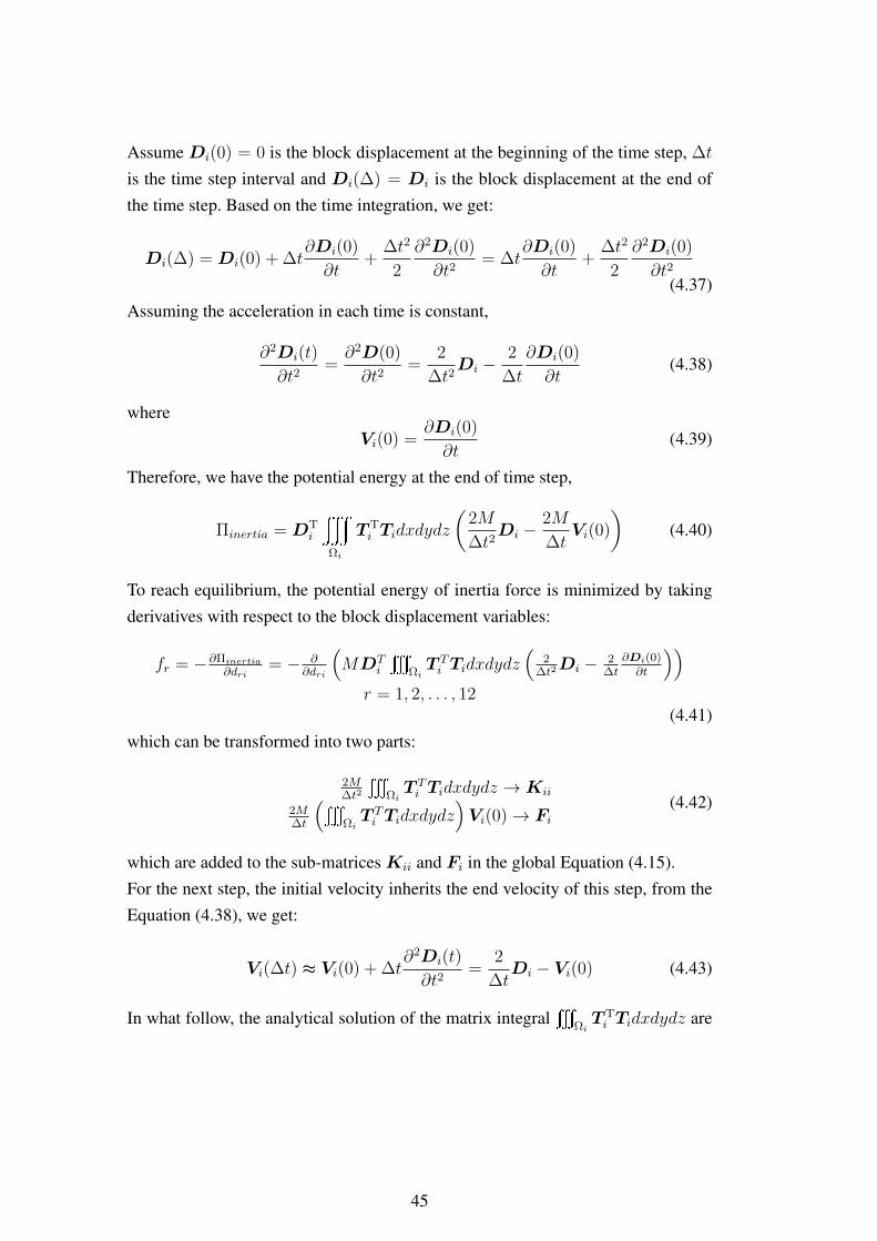
Assume Di(0) = 0 is the block displacement at the beginning of the time step, ∆t
is the time step interval and Di(∆) = Di is the block displacement at the end ofthe time step. Based on the time integration, we get:
Di(∆) = Di(0) + ∆t∂Di(0)
∂t+
∆t2
2
∂2Di(0)
∂t2= ∆t
∂Di(0)
∂t+
∆t2
2
∂2Di(0)
∂t2(4.37)
Assuming the acceleration in each time is constant,
∂2Di(t)
∂t2=∂2D(0)
∂t2=
2
∆t2Di −
2
∆t
∂Di(0)
∂t(4.38)
whereVi(0) =
∂Di(0)
∂t(4.39)
Therefore, we have the potential energy at the end of time step,
Πinertia = DTi
y
Ωi
T Ti Tidxdydz
(2M
∆t2Di −
2M
∆tVi(0)
)(4.40)
To reach equilibrium, the potential energy of inertia force is minimized by takingderivatives with respect to the block displacement variables:
fr = −∂Πinertia
∂dri= − ∂
∂dri
(MDT
i
tΩiT Ti Tidxdydz
(2
∆t2Di − 2
∆t∂Di(0)∂t
))r = 1, 2, . . . , 12
(4.41)which can be transformed into two parts:
2M∆t2
tΩiT Ti Tidxdydz →Kii
2M∆t
(tΩiT Ti Tidxdydz
)Vi(0)→ Fi
(4.42)
which are added to the sub-matricesKii and Fi in the global Equation (4.15).For the next step, the initial velocity inherits the end velocity of this step, from theEquation (4.38), we get:
Vi(∆t) ≈ Vi(0) + ∆t∂2Di(t)
∂t2=
2
∆tDi − Vi(0) (4.43)
In what follow, the analytical solution of the matrix integralt
ΩiT Ti Tidxdydz are
45
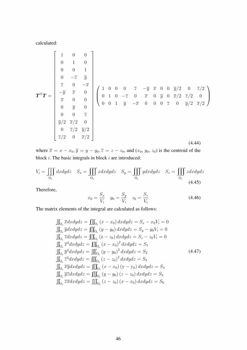
calculated:
T TT =
1 0 0
0 1 0
0 0 1
0 −z y
z 0 −x−y x 0
x 0 0
0 y 0
0 0 z
y/2 x/2 0
0 z/2 y/2
z/2 0 x/2
1 0 0 0 z −y x 0 0 y/2 0 z/2
0 1 0 −z 0 x 0 y 0 x/2 z/2 0
0 0 1 y −x 0 0 0 z 0 y/2 x/2
(4.44)where x = x − x0, y = y − y0, z = z − z0, and (x0, y0, z0) is the centroid of theblock i. The basic integrals in block i are introduced:
Vi =y
Ωi
dxdydz Sx =y
Ωi
xdxdydz Sy =y
Ωi
ydxdydz Sz =y
Ωi
zdxdydz
(4.45)Therefore,
x0 =SxVi
y0 =SyVi
z0 =SzVi
(4.46)
The matrix elements of the integral are calculated as follows:
sΩixdxdydz =
tΩi
(x− x0) dxdydz = Sx − x0Vi = 0sΩiydxdydz =
tΩi
(y − y0) dxdydz = Sy − y0Vi = 0sΩizdxdydz =
tΩi
(z− z0) dxdydz = Sz − z0Vi = 0sΩix2dxdydz =
tΩi
(x− x0)2 dxdydz = S1sΩiy2dxdydz =
tΩi
(y − y0)2 dxdydz = S2sΩiz2dxdydz =
tΩi
(z − z0)2 dxdydz = S3sΩixydxdydz =
tΩi
(x− x0) (y − y0) dxdydz = S4sΩiyzdxdydz =
tΩi
(y − y0) (z − z0) dxdydz = S5sΩizxdxdydz =
tΩi
(z − z0) (x− x0) dxdydz = S6
(4.47)
46
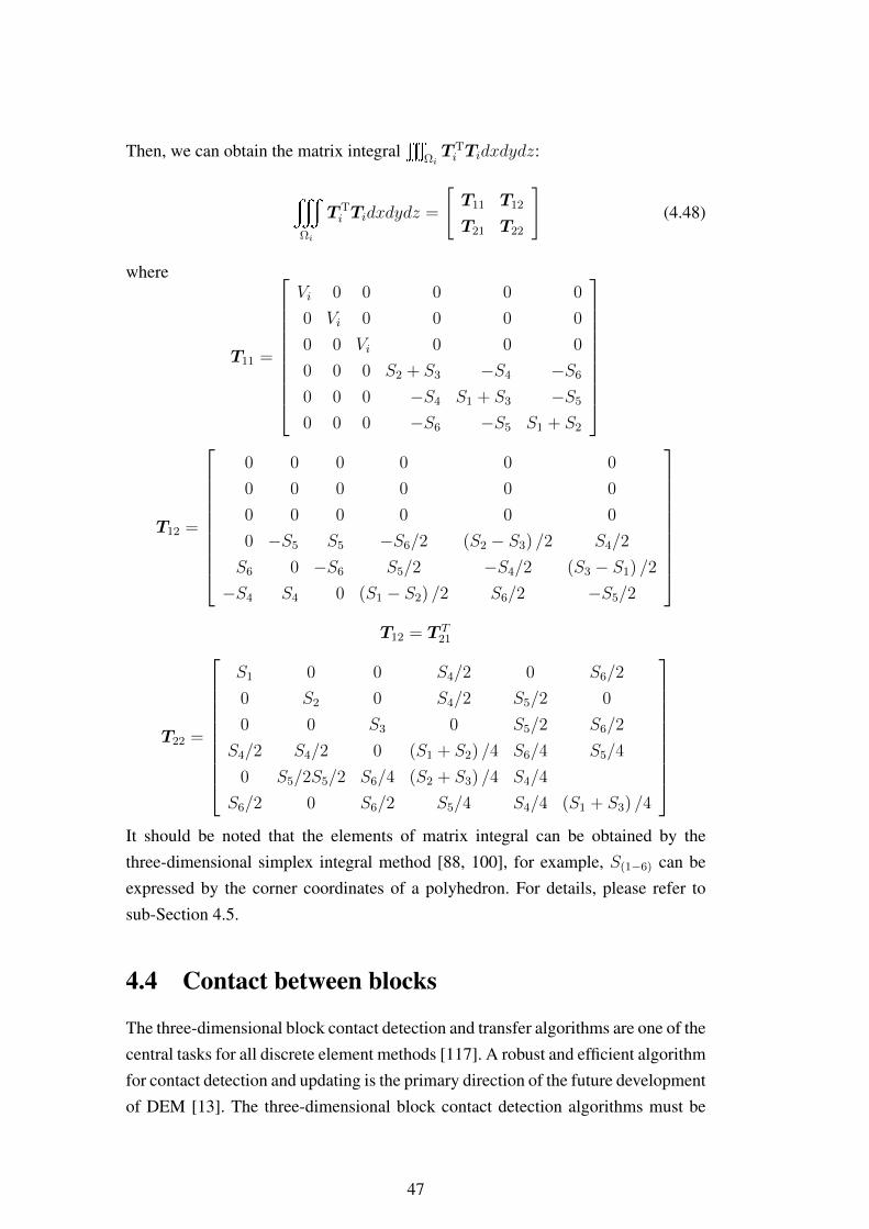
Then, we can obtain the matrix integralt
ΩiT Ti Tidxdydz:
y
Ωi
T Ti Tidxdydz =
[T11 T12
T21 T22
](4.48)
where
T11 =
Vi 0 0 0 0 0
0 Vi 0 0 0 0
0 0 Vi 0 0 0
0 0 0 S2 + S3 −S4 −S6
0 0 0 −S4 S1 + S3 −S5
0 0 0 −S6 −S5 S1 + S2
T12 =
0 0 0 0 0 0
0 0 0 0 0 0
0 0 0 0 0 0
0 −S5 S5 −S6/2 (S2 − S3) /2 S4/2
S6 0 −S6 S5/2 −S4/2 (S3 − S1) /2
−S4 S4 0 (S1 − S2) /2 S6/2 −S5/2
T12 = T T
21
T22 =
S1 0 0 S4/2 0 S6/2
0 S2 0 S4/2 S5/2 0
0 0 S3 0 S5/2 S6/2
S4/2 S4/2 0 (S1 + S2) /4 S6/4 S5/4
0 S5/2S5/2 S6/4 (S2 + S3) /4 S4/4
S6/2 0 S6/2 S5/4 S4/4 (S1 + S3) /4
It should be noted that the elements of matrix integral can be obtained by thethree-dimensional simplex integral method [88, 100], for example, S(1−6) can beexpressed by the corner coordinates of a polyhedron. For details, please refer tosub-Section 4.5.
4.4 Contact between blocks
The three-dimensional block contact detection and transfer algorithms are one of thecentral tasks for all discrete element methods [117]. A robust and efficient algorithmfor contact detection and updating is the primary direction of the future developmentof DEM [13]. The three-dimensional block contact detection algorithms must be
47

used to judge contact types and locations and the appropriate state of each contact,which can be open, sliding or locked [93]. The direct method was used in the origin2D-DDA method; however, this method is not suitable for 3D-DDA due to the largecomputational effort; therefore, in this thesis, the Common-Plane Method (CPM) isintroduced to apply in the 3D-DDA program.
4.4.1 Common-Plane Method
The three-dimensional contact detection of polyhedral blocks is classified into sixbasic types [118]: vertex-to-vertex, edge-to-face, face-to-face, vertex-to-vertex, vertex-to-edge, and edge-to-edge, as shown in Figure 4.1.
Figure 4.1: Basic contact types between two 3-D blocks
Barbosa et al. [119] introduced a simple algorithm for contact detection betweenpolyhedrons that requires detecting all the vertices, edges and faces of blocks. Thetotal detection number N is shown in Equation (4.49). The algorithm has a highcomputational complexity of order O(n2), with n being the number of blocks.
N =n∏i=1
(vi + ei + fi) (4.49)
Although we can reduce the detection number according to classify contact types[120], for example, three and more edge-face contacts at some point can be classi-fied as edge-edge contact, the calculation amount is still very large. For DDA anal-
48

ysis, the direct method is extremely time consuming and not adopted for practicalproblem.Cundall [121] introduced the Common-Plane Method (CPM). A Common-Plane(CP) is a plane that, in some sense, bisects the space between the two contactingblocks. If the two blocks are in contact, then both will intersect the CP, and ifthey are not in contact, then neither intersects the CP. As a result of using CP,the expensive block-to-block contact detection problem reduces to a much fasterplane-to-block contact detection problem. Once the CP is established between twoblocks, the normal to the CP defines the direction of the contact normal, which inturn defines the direction of the normal contact force between the two blocks. Thisis especially advantageous for vertex-to-vertex or edge-to vertex contacts, where thedefinition of the contact normal is a non-trivial problem. This method has the com-plexity of order O(n) and is widely used in some 3D DEM codes [122, 123, 124].In this thesis, we applied the CPM technique to the 3D-DDA program.
4.4.1.1 Algorithm to position the Common-Plane
The CP is defined by two vectors (a) the normal unit vector n of the common-planeand (b) position vector VC where PC is any point at the common plane [122], asshown in Figure 4.2. Assume the PA and PB are one of vertex of two polygons Aand B, VA and VB are the position vector, the distance dA and dB can be expressedas:
Figure 4.2: Definition of distances and sign convention of a point to a plane.
dA = max n · (VA − VC) dA < 0
dB = min n · (VB − VC) dB > 0(4.50)
where VA, VB and VC are the vectors from centroid O to point PA, PB and PC .
49
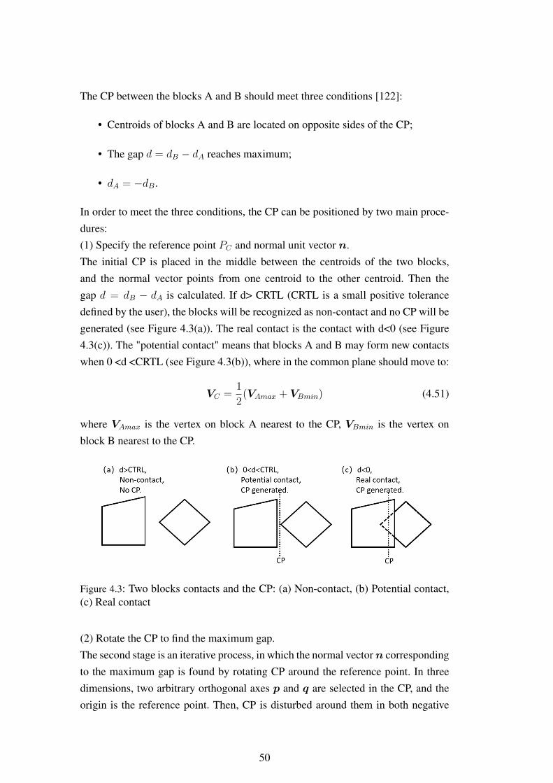
The CP between the blocks A and B should meet three conditions [122]:
• Centroids of blocks A and B are located on opposite sides of the CP;
• The gap d = dB − dA reaches maximum;
• dA = −dB.
In order to meet the three conditions, the CP can be positioned by two main proce-dures:(1) Specify the reference point PC and normal unit vector n.The initial CP is placed in the middle between the centroids of the two blocks,and the normal vector points from one centroid to the other centroid. Then thegap d = dB − dA is calculated. If d> CRTL (CRTL is a small positive tolerancedefined by the user), the blocks will be recognized as non-contact and no CP will begenerated (see Figure 4.3(a)). The real contact is the contact with d<0 (see Figure4.3(c)). The "potential contact" means that blocks A and B may form new contactswhen 0 <d <CRTL (see Figure 4.3(b)), where in the common plane should move to:
VC =1
2(VAmax + VBmin) (4.51)
where VAmax is the vertex on block A nearest to the CP, VBmin is the vertex onblock B nearest to the CP.
Figure 4.3: Two blocks contacts and the CP: (a) Non-contact, (b) Potential contact,(c) Real contact
(2) Rotate the CP to find the maximum gap.The second stage is an iterative process, in which the normal vectorn correspondingto the maximum gap is found by rotating CP around the reference point. In threedimensions, two arbitrary orthogonal axes p and q are selected in the CP, and theorigin is the reference point. Then, CP is disturbed around them in both negative
50
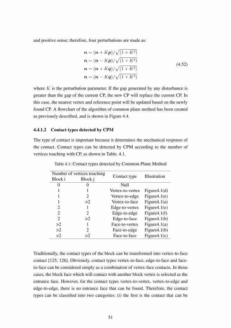
and positive sense; therefore, four perturbations are made as:
n = (n+Kp)/√
(1 +K2)
n = (n−Kp)/√
(1 +K2)
n = (n+Kq)/√
(1 +K2)
n = (n−Kq)/√
(1 +K2)
(4.52)
where K is the perturbation parameter. If the gap generated by any disturbance isgreater than the gap of the current CP, the new CP will replace the current CP. Inthis case, the nearest vertex and reference point will be updated based on the newlyfound CP. A flowchart of the algorithm of common plane method has been createdas previously described, and is shown in Figure 4.4.
4.4.1.2 Contact types detected by CPM
The type of contact is important because it determines the mechanical response ofthe contact. Contact types can be detected by CPM according to the number ofvertices touching with CP, as shown in Table. 4.1.
Table 4.1: Contact types detected by Common-Plane Method
Number of vertices touchingContact type Illustration
Block i Block j0 0 Null1 1 Vertex-to-vertex Figure4.1(d)1 2 Vertex-to-edge Figure4.1(e)1 >2 Vertex-to-face Figure4.1(a)2 1 Edge-to-vertex Figure4.1(e)2 2 Edge-to-edge Figure4.1(f)2 >2 Edge-to-face Figure4.1(b)
>2 1 Face-to-vertex Figure4.1(a)>2 2 Face-to-edge Figure4.1(b)>2 >2 Face-to-face Figure4.1(c)
Traditionally, the contact types of the block can be transformed into vertex-to-facecontact [125, 126]. Obviously, contact types vertex-to-face, edge-to-face and face-to-face can be considered simply as a combination of vertex-face contacts. In thosecases, the block face which will contact with another block vertex is selected as theentrance face. However, for the contact types vertex-to-vertex, vertex-to-edge andedge-to-edge, there is no entrance face that can be found. Therefore, the contacttypes can be classified into two categories: (i) the first is the contact that can be
51
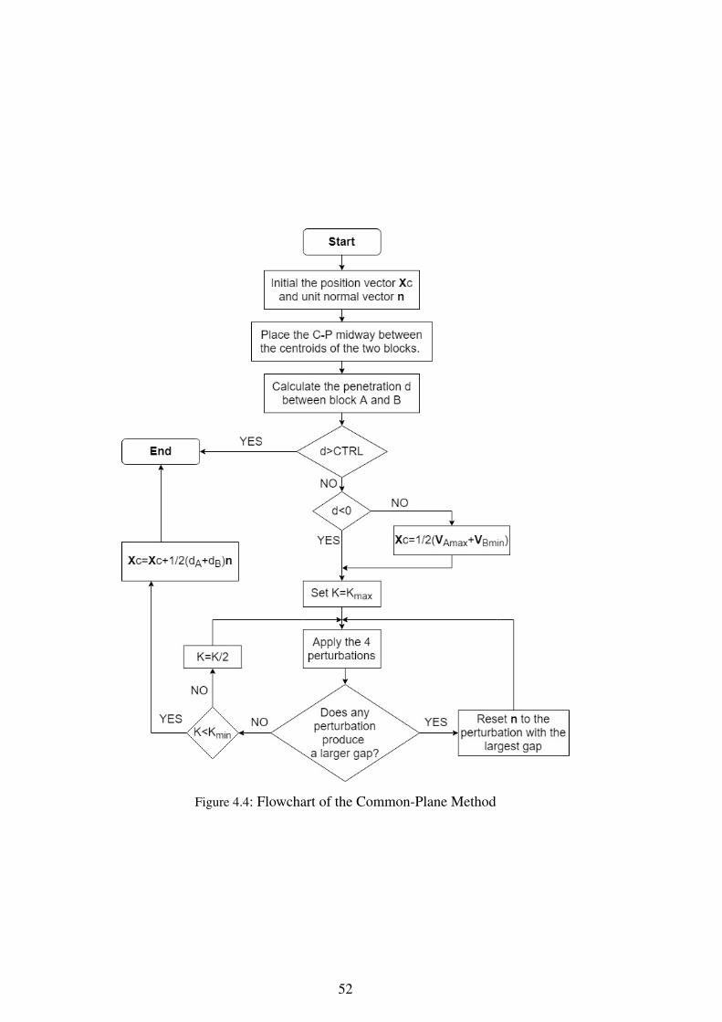
Figure 4.4: Flowchart of the Common-Plane Method
52
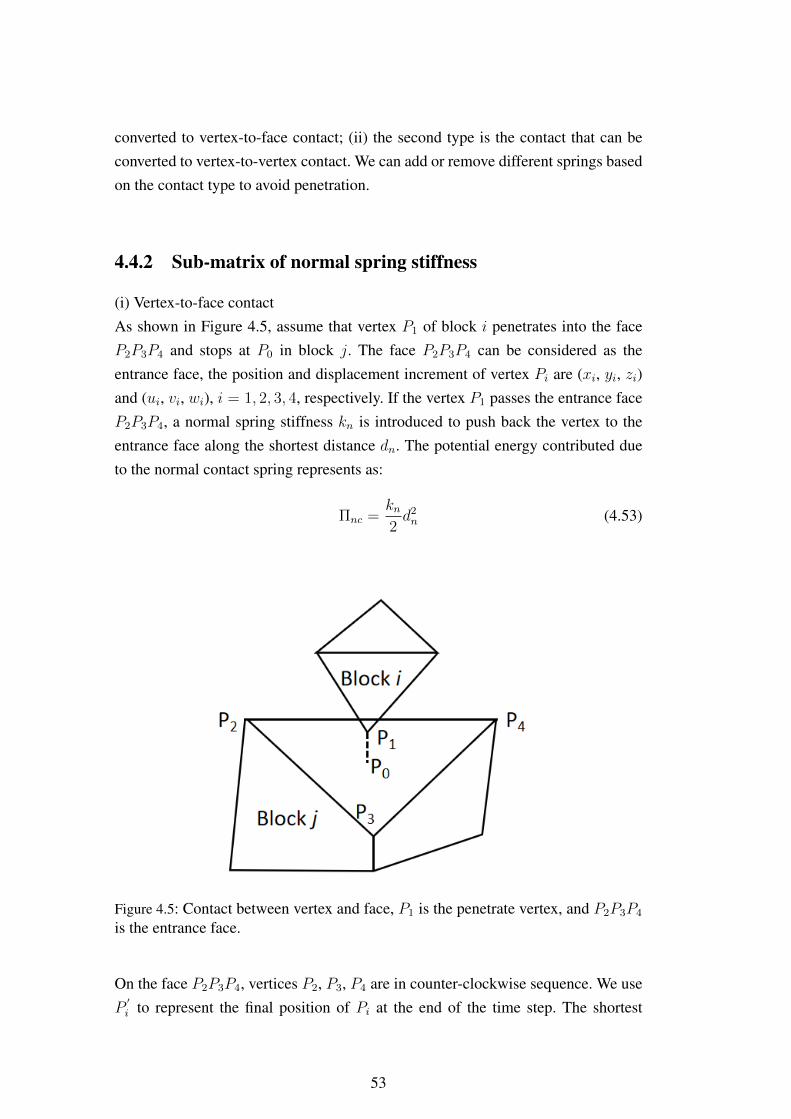
converted to vertex-to-face contact; (ii) the second type is the contact that can beconverted to vertex-to-vertex contact. We can add or remove different springs basedon the contact type to avoid penetration.
4.4.2 Sub-matrix of normal spring stiffness
(i) Vertex-to-face contactAs shown in Figure 4.5, assume that vertex P1 of block i penetrates into the faceP2P3P4 and stops at P0 in block j. The face P2P3P4 can be considered as theentrance face, the position and displacement increment of vertex Pi are (xi, yi, zi)and (ui, vi, wi), i = 1, 2, 3, 4, respectively. If the vertex P1 passes the entrance faceP2P3P4, a normal spring stiffness kn is introduced to push back the vertex to theentrance face along the shortest distance dn. The potential energy contributed dueto the normal contact spring represents as:
Πnc =kn2d2n (4.53)
Figure 4.5: Contact between vertex and face, P1 is the penetrate vertex, and P2P3P4
is the entrance face.
On the face P2P3P4, vertices P2, P3, P4 are in counter-clockwise sequence. We useP
′i to represent the final position of Pi at the end of the time step. The shortest
53
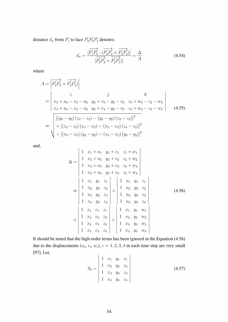
distance dn from P′1 to face P ′
2P′3P
′4 denotes:
dn =[−−→P
′1P
′2 · (−−→P
′2P
′3 ×−−→P
′2P
′4)]
|−−→P
′2P
′3 ×−−→P
′2P
′4)|
=∆
A(4.54)
where
A =
∣∣∣∣−−→P′
2P′
3 ×−−→P
′
2P′
4)
∣∣∣∣=
∣∣∣∣∣∣∣i j k
x3 + u3 − x2 − u2 y3 + v3 − y2 − v2 z3 + w3 − z2 − w2
x4 + u4 − x2 − u2 y4 + v4 − y2 − v2 z4 + w4 − z2 − w2
∣∣∣∣∣∣∣≈
√√√√√√√[(y3 − y2) (z4 − z2)− (y4 − y2) (z3 − z2)]2
+ [(z3 − z2) (x4 − x2)− (x3 − x2) (z4 − z2)]2
+ [(x3 − x2) (y4 − y2)− (x4 − x2) (y3 − y2)]2
(4.55)
and,
∆ =
∣∣∣∣∣∣∣∣∣∣1 x1 + u1 y1 + v1 z1 + w1
1 x2 + u2 y2 + v2 z2 + w2
1 x3 + u3 y3 + v3 z3 + w3
1 x4 + u4 y4 + v4 z4 + w4
∣∣∣∣∣∣∣∣∣∣≈
∣∣∣∣∣∣∣∣∣∣1 x1 y1 z1
1 x2 y2 z2
1 x3 y3 z3
1 x4 y4 z4
∣∣∣∣∣∣∣∣∣∣+
∣∣∣∣∣∣∣∣∣∣1 u1 y1 z1
1 u2 y2 z2
1 u3 y3 z3
1 u4 y4 z4
∣∣∣∣∣∣∣∣∣∣+
∣∣∣∣∣∣∣∣∣∣1 x1 v1 z1
1 x2 v2 z2
1 x3 v3 z3
1 x4 v4 z4
∣∣∣∣∣∣∣∣∣∣+
∣∣∣∣∣∣∣∣∣∣1 x1 y1 w1
1 x2 y2 w2
1 x3 y3 w3
1 x4 y4 w4
∣∣∣∣∣∣∣∣∣∣
(4.56)
It should be noted that the high-order terms has been ignored in the Equation (4.56)due to the displacements (ui, vi, wi), i = 1, 2, 3, 4 in each time step are very small[97]. Let,
S0 =
∣∣∣∣∣∣∣∣∣∣1 x1 y1 z1
1 x2 y2 z2
1 x3 y3 z3
1 x4 y4 z4
∣∣∣∣∣∣∣∣∣∣(4.57)
54
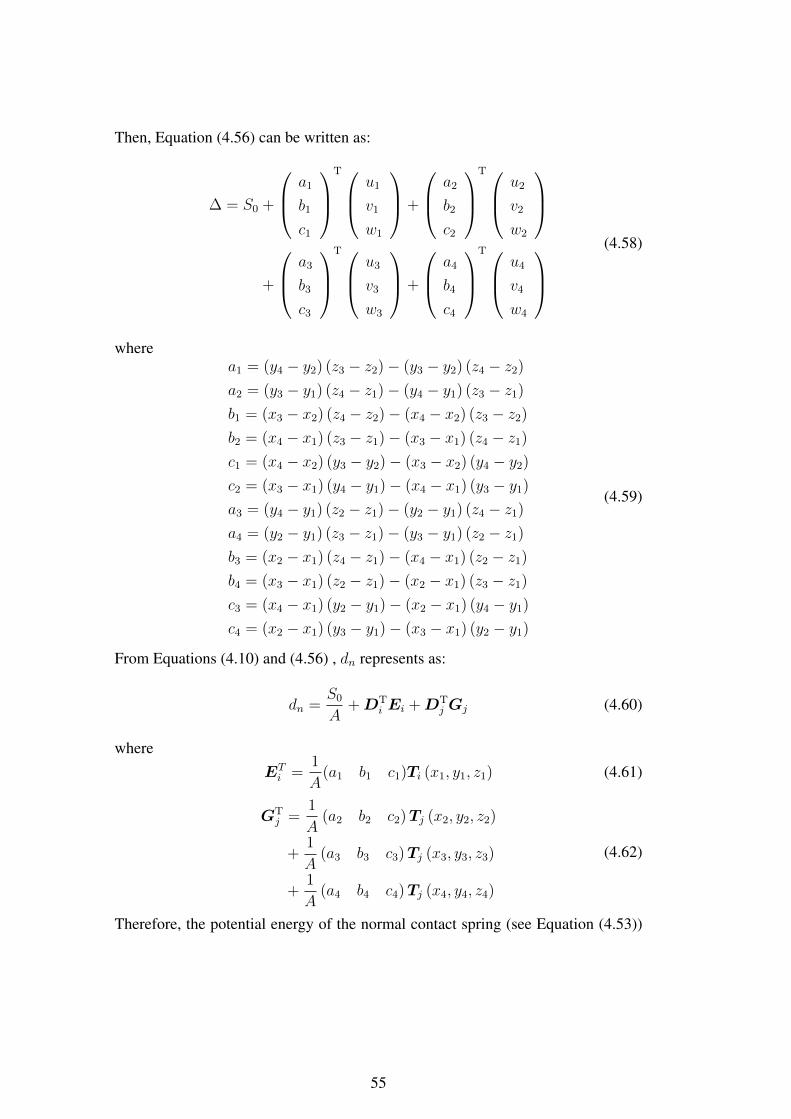
Then, Equation (4.56) can be written as:
∆ = S0 +
a1
b1
c1
T u1
v1
w1
+
a2
b2
c2
T u2
v2
w2
+
a3
b3
c3
T u3
v3
w3
+
a4
b4
c4
T u4
v4
w4
(4.58)
wherea1 = (y4 − y2) (z3 − z2)− (y3 − y2) (z4 − z2)
a2 = (y3 − y1) (z4 − z1)− (y4 − y1) (z3 − z1)
b1 = (x3 − x2) (z4 − z2)− (x4 − x2) (z3 − z2)
b2 = (x4 − x1) (z3 − z1)− (x3 − x1) (z4 − z1)
c1 = (x4 − x2) (y3 − y2)− (x3 − x2) (y4 − y2)
c2 = (x3 − x1) (y4 − y1)− (x4 − x1) (y3 − y1)
a3 = (y4 − y1) (z2 − z1)− (y2 − y1) (z4 − z1)
a4 = (y2 − y1) (z3 − z1)− (y3 − y1) (z2 − z1)
b3 = (x2 − x1) (z4 − z1)− (x4 − x1) (z2 − z1)
b4 = (x3 − x1) (z2 − z1)− (x2 − x1) (z3 − z1)
c3 = (x4 − x1) (y2 − y1)− (x2 − x1) (y4 − y1)
c4 = (x2 − x1) (y3 − y1)− (x3 − x1) (y2 − y1)
(4.59)
From Equations (4.10) and (4.56) , dn represents as:
dn =S0
A+DT
i Ei +DTj Gj (4.60)
whereETi =
1
A(a1 b1 c1)Ti (x1, y1, z1) (4.61)
GTj =
1
A(a2 b2 c2)Tj (x2, y2, z2)
+1
A(a3 b3 c3)Tj (x3, y3, z3)
+1
A(a4 b4 c4)Tj (x4, y4, z4)
(4.62)
Therefore, the potential energy of the normal contact spring (see Equation (4.53))
55
becomes:
Πnc =kn2d2n =
kn2
(S0
A+DT
i Ei +DTj Gj
)2
=kn2
(S0
A
)2
+kn2
(DT
i EiETi Di +DT
j GjGTjDj
)+ kn
S0
A
(DT
i Ei +DTj Gj
)+ knD
Ti EiG
TjDj
(4.63)
Taking the derivative of Πnc, four 12 × 12 sub-matrices and two 12 × 1 sub-matrices can be obtained, which are then added to the sub-matrices Kii, Kij , Kji,Kjj , Fi and Fj of the global Equation (4.15), respectively.• The derivative of Πnc:
Krs =∂2Πnc
∂dri∂dsi= knEiE
Ti →Kii r, s = 1, 2, 3 · · · 12 (4.64)
is added to sub-matrixKii.• The derivative of Πnc:
Krs =∂2Πnc
∂dri∂dsj= knEiG
Tj →Kij r, s = 1, 2, 3 · · · 12 (4.65)
is added to sub-matrixKij .• The derivative of Πnc:
Krs =∂2Πnc
∂drj∂dsi= knGjE
Ti →Kij r, s = 1, 2, 3 · · · 12 (4.66)
is added to sub-matrixKji.• The derivative of Πn:
Krs =∂2Πnc
∂drj∂dsj= knGjG
Tj →Kjj r, s = 1, 2, 3 · · · 12 (4.67)
• The derivative of Πnc:
fr = −∂Πnc(0)
∂dri= −kn
S0
AEi → Fi r = 1, 2, 3 · · · 12 (4.68)
is added to sub-matrix Fi.• The derivative of Πnc:
fr = −∂Πnc(0)
∂drj= −kn
S0
AGj → Fj r = 1, 2, 3 · · · 12 (4.69)
56
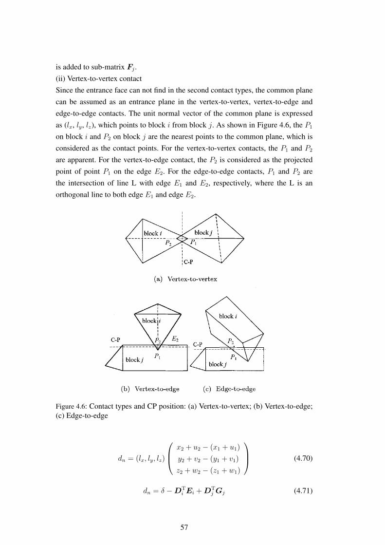
is added to sub-matrix Fj .(ii) Vertex-to-vertex contactSince the entrance face can not find in the second contact types, the common planecan be assumed as an entrance plane in the vertex-to-vertex, vertex-to-edge andedge-to-edge contacts. The unit normal vector of the common plane is expressedas (lx, ly, lz), which points to block i from block j. As shown in Figure 4.6, the P1
on block i and P2 on block j are the nearest points to the common plane, which isconsidered as the contact points. For the vertex-to-vertex contacts, the P1 and P2
are apparent. For the vertex-to-edge contact, the P2 is considered as the projectedpoint of point P1 on the edge E2. For the edge-to-edge contacts, P1 and P2 arethe intersection of line L with edge E1 and E2, respectively, where the L is anorthogonal line to both edge E1 and edge E2.
Figure 4.6: Contact types and CP position: (a) Vertex-to-vertex; (b) Vertex-to-edge;(c) Edge-to-edge
dn = (lx, ly, lz)
x2 + u2 − (x1 + u1)
y2 + v2 − (y1 + v1)
z2 + w2 − (z1 + w1)
(4.70)
dn = δ −DTi Ei +DT
j Gj (4.71)
57
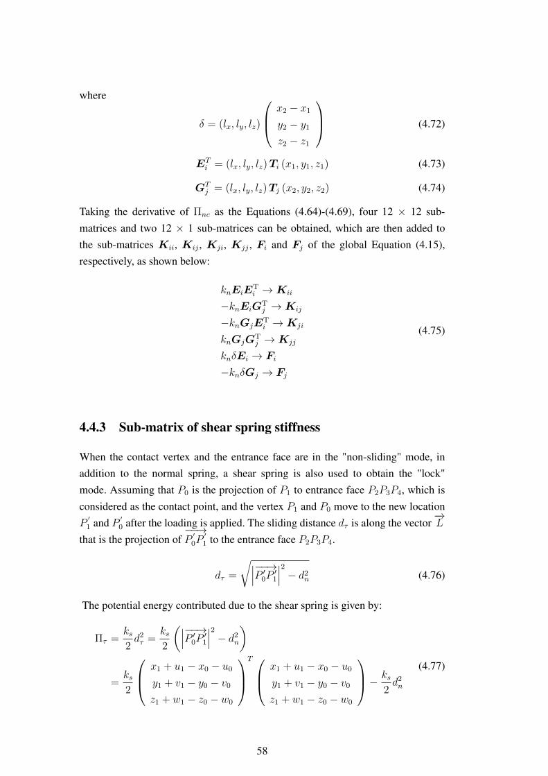
where
δ = (lx, ly, lz)
x2 − x1
y2 − y1
z2 − z1
(4.72)
ETi = (lx, ly, lz)Ti (x1, y1, z1) (4.73)
GTj = (lx, ly, lz)Tj (x2, y2, z2) (4.74)
Taking the derivative of Πnc as the Equations (4.64)-(4.69), four 12 × 12 sub-matrices and two 12 × 1 sub-matrices can be obtained, which are then added tothe sub-matrices Kii, Kij , Kji, Kjj , Fi and Fj of the global Equation (4.15),respectively, as shown below:
knEiETi →Kii
−knEiGTj →Kij
−knGjETi →Kji
knGjGTj →Kjj
knδEi → Fi
−knδGj → Fj
(4.75)
4.4.3 Sub-matrix of shear spring stiffness
When the contact vertex and the entrance face are in the "non-sliding" mode, inaddition to the normal spring, a shear spring is also used to obtain the "lock"mode. Assuming that P0 is the projection of P1 to entrance face P2P3P4, which isconsidered as the contact point, and the vertex P1 and P0 move to the new locationP
′1 and P ′
0 after the loading is applied. The sliding distance dτ is along the vector−→L
that is the projection of−−→P
′0P
′1 to the entrance face P2P3P4.
dτ =
√∣∣∣−−→P ′0P′1
∣∣∣2 − d2n (4.76)
The potential energy contributed due to the shear spring is given by:
Πτ =ks2d2τ =
ks2
(∣∣∣−−→P ′0P′1
∣∣∣2 − d2n
)
=ks2
x1 + u1 − x0 − u0
y1 + v1 − y0 − v0
z1 + w1 − z0 − w0
T x1 + u1 − x0 − u0
y1 + v1 − y0 − v0
z1 + w1 − z0 − w0
− ks2d2n
(4.77)
58
Figure 4.7: Contact vertex and the entrance face, and the position of shear spring
From Equations (4.71) and (4.77), we can get:
Πτ =ks2
([x1 − x0 y1 − y0 z1 − z0
]+DT
i TTi −DT
j TTj
) x1 − x0
y1 − y0
z1 − z0
+ TiDi − TjDj
− ks2
(S0
A+DT
i Ei +DTj Gj
)2 (4.78)
Taking the derivative of Πτ , four 12× 12 sub-matrices and two 12× 1 sub-matricescan be obtained, which are then added to the sub-matrices Kii, Kij , Kji, Kjj , Fiand Fj of the global Equation (4.15), respectively.• The derivative of Πτ :
krs =∂2Πτ
∂dri∂dsi
=ksTTi Ti − ksET
i Ei →Kii
(4.79)
which is a 12 × 12 sub-matrix and added toKii of the global Equation (4.15).• The derivative of Πτ :
krs =∂2Πτ
∂dri∂dsj
=− ksT Ti Tj − ksET
i Gj →Kij
(4.80)
59
which is a 12 × 12 sub-matrix and added toKij of the global Equation (4.15).• The derivative of Πτ :
krs =∂2Πτ
∂drj∂dsi
=− ksT Tj Ti − ksGT
j Ei →Kji
(4.81)
which is a 12 × 12 sub-matrix and added toKji of the global Equation (4.15).• The derivative of Πτ :
krs =∂2Πτ
∂drj∂dsj
=ksTTj Tj − ksGT
j Gj →Kjj
(4.82)
which is a 12 × 12 sub-matrix and added toKjj of the global Equation (4.15).• The derivative of the potential energy Πτ of the force at P0 on block i is:
fr = −∂Πτ (0)
∂dri
= −ksT Ti
x1 − x0
y1 − y0
z1 − z0
+ksS0
AETi → Fi
(4.83)
which is a 12 × 1 sub-matrix and added to Fi of the global Equation (4.15).• The derivative of the potential energy Πτ of the force at P0 on block j is:
fr =∂Πτ (0)
∂drj
= −ksT Tj
x1 − x0
y1 − y0
z1 − z0
+ksS0
AGTj → Fj
(4.84)
which is a 12 × 1 sub-matrix and added to Fj of the global Equation (4.15).For the second contact types (see Figure 4.6), the contact points are P1 of block iand P2 of block j. The potential energy of the shear spring is:
Πτ =ks2d2τ =
ks2
(∣∣∣−−→P ′2P′1
∣∣∣2 − d2n
)
=ks2
x1 + u1 − x2 − u2
y1 + v1 − y2 − v2
z1 + w1 − z2 − w2
T x1 + u1 − x2 − u2
y1 + v1 − y2 − v2
z1 + w1 − z2 − w2
− ks2d2n
(4.85)
60
Taking the derivative of Πτ as the Equations (4.79)-(4.84), four 12 × 12 sub-matrices and two 12 × 1 sub-matrices can be obtained, which are then added tothe sub-matrices Kii, Kij , Kji, Kjj , Fi and Fj of the global Equation (4.15),respectively, as shown below:
ksTTi Ti − ksET
i Ei →Kii
−ksT Ti Tj + ksE
Ti Gj →Kij
−ksT Tj Ti + ksG
Tj Ei →Kji
ksTTj Tj − ksGT
jGj →Kjj
−ksT Ti
x1 − x2
y1 − y2
z1 − z2
− ksδETi → Fi
ksTTj
x1 − x2
y1 − y2
z1 − z2
+ ksδGTj → Fj
(4.86)
where δ, Ei andGj are same as shown in Equations (4.72)-(4.74).
4.4.4 Sub-matrix of friction spring stiffness
The frictional forces should be considered when the contact is at the sliding state[127]. For the sliding state, the normal spring and the friction spring need to beadded. Based on Coulomb’s law, the friction force is:
Ff = kn|dn|tan(φ) + Cf (4.87)
where kn is the normal spring stiffness, dn is the normal penetration distance,tan(φ) is the friction coefficient in which φ is the friction angle, and Cf is thecohesion.The frictional force direction
−→L is the projection of
−−→P ′0P
′1 on face P2P3P4 (see
Figure 4.7).
−−→P ′0P
′1 = (x1 + u′1 − x0 − u′0)~i+ (y1 + v′1 − y0 − v′0)~j + (z1 + w′1 − z0 − w′0)~k
(4.88)
61
The unit normal vector−→of of face P2P3P4 can be obtained by:
−→of =
1
A
[(y3 − y2) (z4 − z2)− (y4 − y2) (z3 − z2)]~i
+ [(z3 − z2) (x4 − x2)− (x3 − x2) (z4 − z2)]~j
+ [(x3 − x2) (y4 − y2)− (x4 − x2) (y3 − y2)]~k (4.89)
where the A can be calculated by Equation (4.55). Then the−→L and it’s value
represent as:−→L =
−−→P ′0P
′1 + |dn|
−→of = a~i+ b~j + c~k (4.90)
|−→L | =
√|−−→P ′0P
′1|2 − |dn|2 = dτ (4.91)
where the dn and dτ are determined from the previous iteration, and
a = (x1 + u′1 − x0 − u′0)− a1|dn|A
b = (y1 + v′1 − y0 − v′0)− b1|dn|A
c = (z1 + w′1 − z0 − w′0)− c1|dn|A
(4.92)
where a1, b1, c1 are the same as Equation (4.59).The potential energy Πfi contributed by frictional force Ff at P1 of block i is:
Πfi =Ff
|~L|(u1 v1 w1)
a
b
c
=FfdτDT
i TTi
a
b
c
= FfD
Ti Ei
(4.93)
where
Ei =1
dτT Ti
a
b
c
(4.94)
Based on the minimization of potential energy, the derivative of Πfi at zero dis-placement position can be calculated and added to Fi in the global Equation (4.15).
fr = −∂Πfi(0)
∂dri= −FfEi → Fi (4.95)
62
where r=1,2,3,· · · ,12.The potential energy Πfj contributed by frictional force Ff at P1 of block i is:
Πfj = −Ff|~L|
(u1 v1 w1)
a
b
c
= −FfdτDT
j TTj
a
b
c
= −FfDT
j Gj
(4.96)
The derivative of Πfj at zero displacement position can be calculated added to Fjin the global Equation (4.15).
fr = −∂Πfj(0)
∂drj= FfGj → Fj (4.97)
where r=1,2,3,· · · ,12, and
Gj =1
dτT Tj
a
b
c
(4.98)
4.4.5 Open-close iterations
Each contact has three possible states: open, sliding and lock. These states can bedetermined by relationships between normal component Fn and shear componentFs based on the Mohr-Coulomb law.(1) Open stateCondition: when the normal component Fn of contact force is tensile:
Fn = −kndn ≤ 0 (4.99)
where dn < 0 means penetration occurs.Operation: no normal and shear spring should be added.
(2) Sliding stateCondition: when the normal component Fn is compressive, and the shear compo-
63
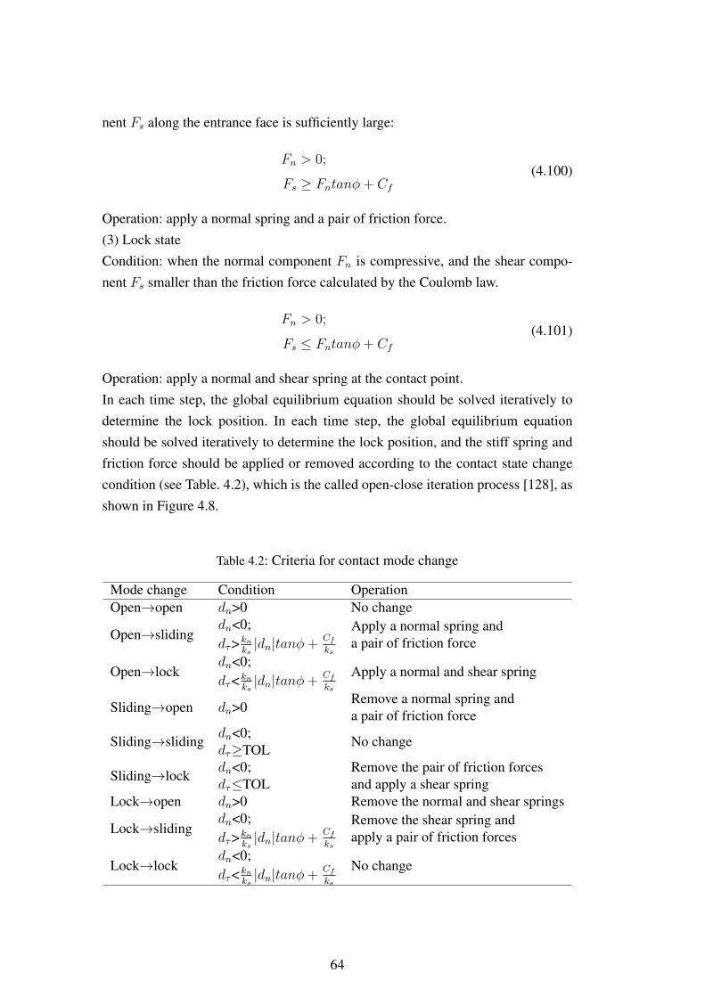
nent Fs along the entrance face is sufficiently large:
Fn > 0;
Fs ≥ Fntanφ+ Cf(4.100)
Operation: apply a normal spring and a pair of friction force.(3) Lock stateCondition: when the normal component Fn is compressive, and the shear compo-nent Fs smaller than the friction force calculated by the Coulomb law.
Fn > 0;
Fs ≤ Fntanφ+ Cf(4.101)
Operation: apply a normal and shear spring at the contact point.In each time step, the global equilibrium equation should be solved iteratively todetermine the lock position. In each time step, the global equilibrium equationshould be solved iteratively to determine the lock position, and the stiff spring andfriction force should be applied or removed according to the contact state changecondition (see Table. 4.2), which is the called open-close iteration process [128], asshown in Figure 4.8.
Table 4.2: Criteria for contact mode change
Mode change Condition OperationOpen→open dn>0 No change
Open→slidingdn<0;dτ>kn
ks|dn|tanφ+
Cf
ks
Apply a normal spring anda pair of friction force
Open→lockdn<0;dτ<kn
ks|dn|tanφ+
Cf
ks
Apply a normal and shear spring
Sliding→open dn>0Remove a normal spring anda pair of friction force
Sliding→slidingdn<0;dτ≥TOL No change
Sliding→lockdn<0;dτ≤TOL
Remove the pair of friction forcesand apply a shear spring
Lock→open dn>0 Remove the normal and shear springs
Lock→slidingdn<0;dτ>kn
ks|dn|tanφ+
Cf
ks
Remove the shear spring andapply a pair of friction forces
Lock→lockdn<0;dτ<kn
ks|dn|tanφ+
Cf
ks
No change
64

where dn and dτ are the normal and shear displacements, calculated by the lastiteration. TOL=0.1 mm is a given limit value.
Figure 4.8: Flowchart of open-close iteration
65
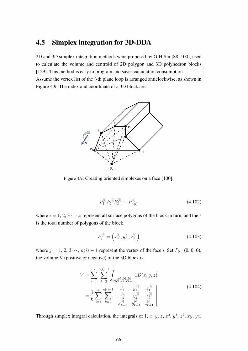
4.5 Simplex integration for 3D-DDA
2D and 3D simplex integration methods were proposed by G-H Shi [88, 100], usedto calculate the volume and centroid of 2D polygon and 3D polyhedron blocks[129]. This method is easy to program and saves calculation consumption.Assume the vertex list of the i-th plane loop is arranged anticlockwise, as shown inFigure 4.9. The index and coordinate of a 3D block are:
Figure 4.9: Creating oriented simplexes on a face [100].
P[i]1 P
[i]2 P
[i]3 . . . P
[i]n(i) (4.102)
where i = 1, 2, 3 · · · ,s represent all surface polygons of the block in turn, and the sis the total number of polygons of the block.
P[i]j =
(x
[i]j , y
[i]j , z
[i]j
)(4.103)
where j = 1, 2, 3· · · , n(i) − 1 represent the vertex of the face i. Set P0 =(0, 0, 0),the volume V (positive or negative) of the 3D block is:
V =s∑i=1
n(i)−1∑k=2
∫p0p
(i]1 p
[i]k p
[i]k+1
1D(x, y, z)
=1
6
s∑i=1
n(i)−1∑k=2
∣∣∣∣∣∣∣x
[i]1 y
[i]1 z
[i]1
x[i]k y
[i]k z
[i]k
x[i]k+1 y
[i]k+1 z
[i]k+1
∣∣∣∣∣∣∣(4.104)
Through simplex integral calculation, the integrals of 1, x, y, z, x2, y2, z2, xy, yz,
66
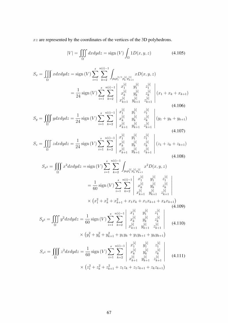
xz are represented by the coordinates of the vertices of the 3D polyhedrons.
|V | =y
Ω
dxdydz = sign (V )
∫Ω
1D(x, y, z) (4.105)
Sx =y
Ω
xdxdydz = sign (V )s∑i=1
n(i)−1∑k=2
∫p0p
[1/11 p
[i]k p
[1]k+1
xD(x, y, z)
=1
24sign (V )
s∑i=1
n(i)−1∑k=2
∣∣∣∣∣∣∣x
[i]1 y
[i]1 z
[i]1
x[i]k y
[i]k z
[i]k
x[i]k+1 y
[i]k+1 z
[i]k+1
∣∣∣∣∣∣∣ (x1 + xk + xk+1)
(4.106)
Sy =y
Ω
ydxdydz =1
24sign (V )
s∑i=1
n(i)−1∑k=2
∣∣∣∣∣∣∣x
[i]1 y
[i]1 z
[i]1
x[i]k y
[i]k z
[i]k
x[i]k+1 y
[i]k+1 z
[i]k+1
∣∣∣∣∣∣∣ (y1 + yk + yk+1)
(4.107)
Sz =y
Ω
zdxdydz =1
24sign (V )
s∑i=1
n(i)−1∑k=2
∣∣∣∣∣∣∣x
[i]1 y
[i]1 z
[i]1
x[i]k y
[i]k z
[i]k
x[i]k+1 y
[i]k+1 z
[i]k+1
∣∣∣∣∣∣∣ (z1 + zk + zk+1)
(4.108)
Sx2 =y
Ω
x2dxdydz = sign (V )s∑i=1
n(i)−1∑k=2
∫p0p
[i]1 p
[i]k p
[i]k+1
x2D(x, y, z)
=1
60sign (V )
s∑i=1
n(i)−1∑k=2
∣∣∣∣∣∣∣x
[i]1 y
[i]1 z
[i]1
x[i]k y
[i]k z
[i]k
x[i]k+1 y
[i]k+1 z
[i]k+1
∣∣∣∣∣∣∣×(x2
1 + x2k + x2
k+1 + x1xk + x1xk+1 + xkxk+1
)(4.109)
Sy2 =y
Ω
y2dxdydz =1
60sign (V )
s∑i=1
n(i)−1∑k=2
∣∣∣∣∣∣∣x
[i]1 y
[i]1 z
[i]1
x[i]k y
[i]k z
[i]k
x[i]k+1 y
[i]k+1 z
[i]k+1
∣∣∣∣∣∣∣×(y2
1 + y2k + y2
k+1 + y1yk + y1yk+1 + ykyk+1
) (4.110)
Sz2 =y
Ω
z2dxdydz =1
60sign (V )
s∑i=1
n(i)−1∑k=2
∣∣∣∣∣∣∣x
[i]1 y
[i]1 z
[i]1
x[i]k y
[i]k z
[i]k
x[i]k+1 y
[i]k+1 z
[i]k+1
∣∣∣∣∣∣∣×(z2
1 + z2k + z2
k+1 + z1zk + z1zk+1 + zkzk+1
) (4.111)
67
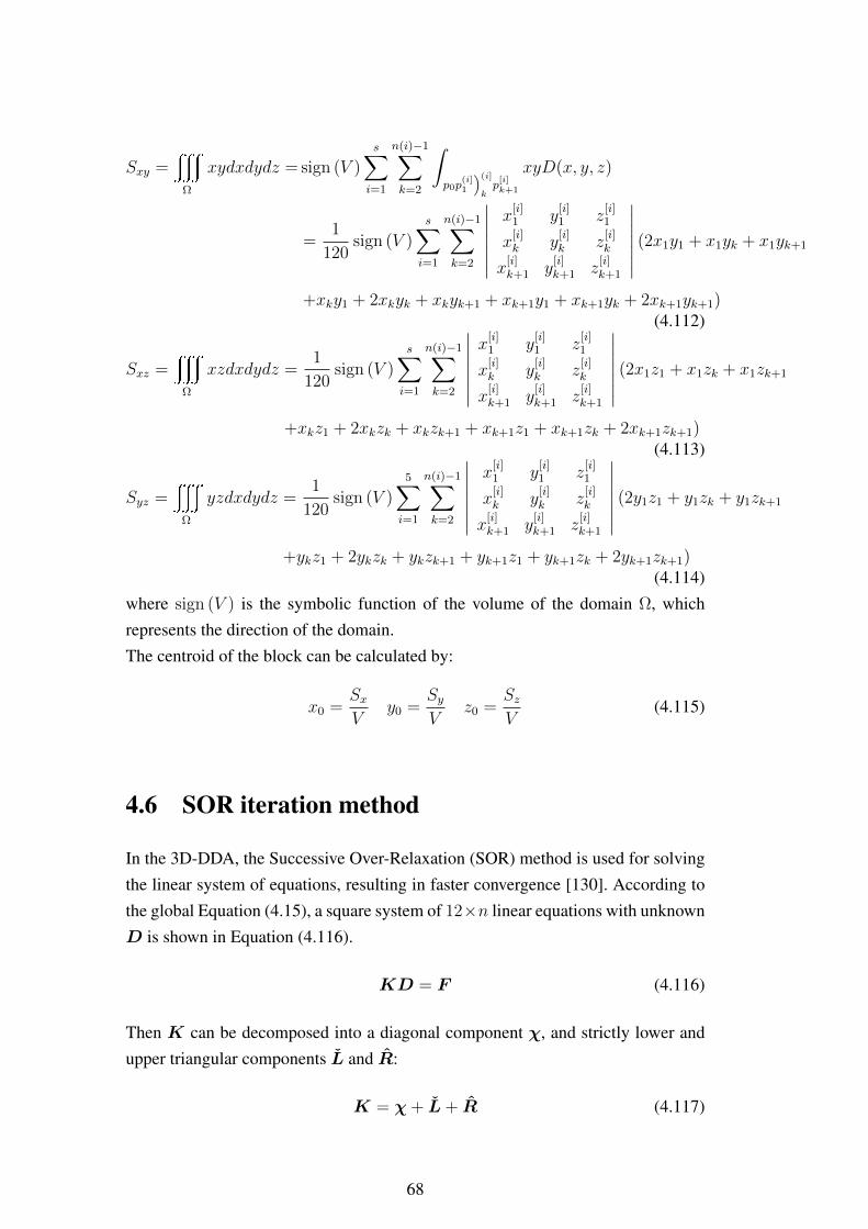
Sxy =y
Ω
xydxdydz = sign (V )s∑i=1
n(i)−1∑k=2
∫p0p
(i]1
)(i]
kp[i]k+1
xyD(x, y, z)
=1
120sign (V )
s∑i=1
n(i)−1∑k=2
∣∣∣∣∣∣∣x
[i]1 y
[i]1 z
[i]1
x[i]k y
[i]k z
[i]k
x[i]k+1 y
[i]k+1 z
[i]k+1
∣∣∣∣∣∣∣ (2x1y1 + x1yk + x1yk+1
+xky1 + 2xkyk + xkyk+1 + xk+1y1 + xk+1yk + 2xk+1yk+1)(4.112)
Sxz =y
Ω
xzdxdydz =1
120sign (V )
s∑i=1
n(i)−1∑k=2
∣∣∣∣∣∣∣x
[i]1 y
[i]1 z
[i]1
x[i]k y
[i]k z
[i]k
x[i]k+1 y
[i]k+1 z
[i]k+1
∣∣∣∣∣∣∣ (2x1z1 + x1zk + x1zk+1
+xkz1 + 2xkzk + xkzk+1 + xk+1z1 + xk+1zk + 2xk+1zk+1)(4.113)
Syz =y
Ω
yzdxdydz =1
120sign (V )
5∑i=1
n(i)−1∑k=2
∣∣∣∣∣∣∣x
[i]1 y
[i]1 z
[i]1
x[i]k y
[i]k z
[i]k
x[i]k+1 y
[i]k+1 z
[i]k+1
∣∣∣∣∣∣∣ (2y1z1 + y1zk + y1zk+1
+ykz1 + 2ykzk + ykzk+1 + yk+1z1 + yk+1zk + 2yk+1zk+1)(4.114)
where sign (V ) is the symbolic function of the volume of the domain Ω, whichrepresents the direction of the domain.The centroid of the block can be calculated by:
x0 =SxV
y0 =SyV
z0 =SzV
(4.115)
4.6 SOR iteration method
In the 3D-DDA, the Successive Over-Relaxation (SOR) method is used for solvingthe linear system of equations, resulting in faster convergence [130]. According tothe global Equation (4.15), a square system of 12×n linear equations with unknownD is shown in Equation (4.116).
KD = F (4.116)
Then K can be decomposed into a diagonal component χ, and strictly lower andupper triangular components L and R:
K = χ+ L+ R (4.117)
68
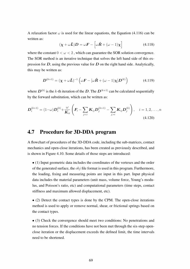
A relaxation factor ω is used for the linear equations, the Equation (4.116) can bewritten as:
(χ+ ωL)D = ωF −[ωR+ (ω − 1)χ
](4.118)
where the constant 0 < ω < 2 , which can guarantee the SOR solution convergence.The SOR method is an iterative technique that solves the left hand side of this ex-pression forD, using the previous value forD on the right hand side. Analytically,this may be written as:
D(k+1) = (χ+ ωL)−1(ωF − [ωR+ (ω − 1)χ]D(k)
)(4.119)
whereD(k) is the k-th iteration of theD. TheD(k+1) can be calculated sequentiallyby the forward substitution, which can be written as:
D(k+1)i = (1−ω)D
(k)i +
ω
Kii
(Fi −
∑j<i
KijD(k+1)j −
∑j>i
KijD(k)j
), i = 1, 2, . . . , n
(4.120)
4.7 Procedure for 3D-DDA program
A flowchart of procedures of the 3D-DDA code, including the sub-matrices, contactmechanics and open-close iterations, has been created as previously described, andis shown in Figure 4.10. Some details of those steps are introduced:
• (1) Input geometric data includes the coordinates of the vertexes and the orderof the generated surface, the obj file format is used in this program. Furthermore,the loading, fixing and measuring points are input in this part. Input physicaldata includes the material parameters (unit mass, volume force, Young’s modu-lus, and Poisson’s ratio, etc) and computational parameters (time steps, contactstiffness and maximum allowed displacement, etc).
• (2) Detect the contact types is done by the CPM. The open-close iterationsmethod is used to apply or remove normal, shear, or frictional springs based onthe contact types.
• (3) Check the convergence should meet two conditions: No penetrations andno tension forces. If the conditions have not been met through the six-step open-close iteration or the displacement exceeds the defined limit, the time intervalsneed to be shortened.
69
Figure 4.10: Flow chart of 3D-DDA procedure.
70
4.8 Concluding remarks
The mathematical formation of the 3D-DDA method was presented in this section,some new numerical technologies were used in programming:
− The CPM was used to detect the contact types, the calculation speed wasgreatly improved and the calculation consumption was saved by comparing theoriginal direct method.
− The soft contact approach instead of the hard penalty method was used in thisthesis to consider the normal and shear contact stiffness.
− The contact was divided in two types, which are vertex-to-face contact andvertex-to-vertex contact, corresponding normal and shear springs as well as fric-tional forces were added based on the contact type.
− During each time step, the global equilibrium equations were solved itera-tively by the SOR method to determine the lock position.
With these improvements, this 3D-DDA code will be able to simulate more con-ditions for discontinuous mediums. And the simulation results can be greatly im-proved for better predictions of their physics.
71

Chapter 5
2D-DDA results application to ballastflight in high speed railways
5.1 Introduction
In this chapter, a numerical model based on the 2D-DDA method is proposed tostudy the ballast flight caused by dropping snow / ice blocks in high-speed railways.The following aspects are emphasized:
• The validation of the proposed model is done by comparing the numericalresults with the experimental results.
• The numerical results show that the velocity, shape and incident angle of snow/ ice block play an important role in the ballast flight. The number and themaximum displacement of ballast particles increase as the train speed increases.
• The incident angle of ice block greatly affects the movement direction ofballast particles.
• The shape of the ice block affects the amount and extent of ballast flight.
5.2 Background
The phenomenon of ballast flight is one of the major problems in high speed bal-lasted track, which has resulted in major maintenance costs and safety concerns.Flying ballast particles may hit the rail, the train body or the passengers throughstations. Furthermore, small particles of ballast may come to rest between the rail-head and the wheels of rail vehicles, which cause substantial local bending damageto the rail [131, 132]. The aerodynamic effect is commonly regarded as the maincause of ballast flight [133, 134]. However, as counted by Saat et al. [135], about50% of ballast flight incidents occur in snow condition. This is because high-speed
73
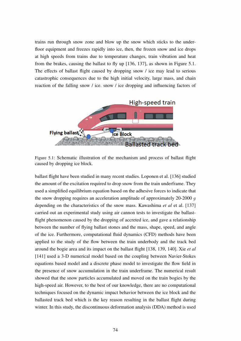
trains run through snow zone and blow up the snow which sticks to the under-floor equipment and freezes rapidly into ice, then, the frozen snow and ice dropsat high speeds from trains due to temperature changes, train vibration and heatfrom the brakes, causing the ballast to fly up [136, 137], as shown in Figure 5.1.The effects of ballast flight caused by dropping snow / ice may lead to seriouscatastrophic consequences due to the high initial velocity, large mass, and chainreaction of the falling snow / ice. snow / ice dropping and influencing factors of
Figure 5.1: Schematic illustration of the mechanism and process of ballast flightcaused by dropping ice block.
ballast flight have been studied in many recent studies. Loponen et al. [136] studiedthe amount of the excitation required to drop snow from the train underframe. Theyused a simplified equilibrium equation based on the adhesive forces to indicate thatthe snow dropping requires an acceleration amplitude of approximately 20-2000 gdepending on the characteristics of the snow mass. Kawashima et al et al. [137]carried out an experimental study using air cannon tests to investigate the ballast-flight phenomenon caused by the dropping of accreted ice, and gave a relationshipbetween the number of flying ballast stones and the mass, shape, speed, and angleof the ice. Furthermore, computational fluid dynamics (CFD) methods have beenapplied to the study of the flow between the train underbody and the track bedaround the bogie area and its impact on the ballast flight [138, 139, 140]. Xie et al
[141] used a 3-D numerical model based on the coupling between Navier-Stokesequations based model and a discrete phase model to investigate the flow field inthe presence of snow accumulation in the train underframe. The numerical resultshowed that the snow particles accumulated and moved on the train bogies by thehigh-speed air. However, to the best of our knowledge, there are no computationaltechniques focused on the dynamic impact behavior between the ice block and theballasted track bed which is the key reason resulting in the ballast flight duringwinter. In this study, the discontinuous deformation analysis (DDA) method is used
74
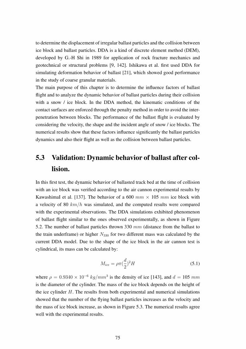
to determine the displacement of irregular ballast particles and the collision betweenice block and ballast particles. DDA is a kind of discrete element method (DEM),developed by G.-H Shi in 1989 for application of rock fracture mechanics andgeotechnical or structural problems [9, 142]. Ishikawa et al. first used DDA forsimulating deformation behavior of ballast [21], which showed good performancein the study of coarse granular materials.The main purpose of this chapter is to determine the influence factors of ballastflight and to analyze the dynamic behavior of ballast particles during their collisionwith a snow / ice block. In the DDA method, the kinematic conditions of thecontact surfaces are enforced through the penalty method in order to avoid the inter-penetration between blocks. The performance of the ballast flight is evaluated byconsidering the velocity, the shape and the incident angle of snow / ice blocks. Thenumerical results show that these factors influence significantly the ballast particlesdynamics and also their flight as well as the collision between ballast particles.
5.3 Validation: Dynamic behavior of ballast after col-lision.
In this first test, the dynamic behavior of ballasted track bed at the time of collisionwith an ice block was verified according to the air cannon experimental results byKawashimaI et al. [137]. The behavior of a 600 mm × 105 mm ice block witha velocity of 80 km/h was simulated, and the computed results were comparedwith the experimental observations. The DDA simulations exhibited phenomenonof ballast flight similar to the ones observed experimentally, as shown in Figure5.2. The number of ballast particles thrown 330 mm (distance from the ballast tothe train underframe) or higher N330 for two different mass was calculated by thecurrent DDA model. Due to the shape of the ice block in the air cannon test iscylindrical, its mass can be calculated by:
Mice = ρπ(d
2)2H (5.1)
where ρ = 0.9340 × 10⁻⁶ kg/mm3 is the density of ice [143], and d = 105 mmis the diameter of the cylinder. The mass of the ice block depends on the height ofthe ice cylinder H . The results from both experimental and numerical simulationsshowed that the number of the flying ballast particles increases as the velocity andthe mass of ice block increase, as shown in Figure 5.3. The numerical results agreewell with the experimental results.
75
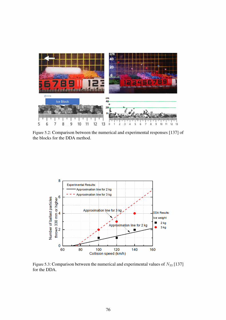
Figure 5.2: Comparison between the numerical and experimental responses [137] ofthe blocks for the DDA method.
Figure 5.3: Comparison between the numerical and experimental values ofN33 [137]for the DDA.
76

5.4 Simulation results
5.4.1 Velocity of ice block
5.4.1.1 Cross section
The ballast shoulder has a width of 500 mm and a height of 100 mm, whereasthe ballast bed has a thickness of 350 mm (see Figure 5.4). Based on the Euro-pean standard: aggregates for railway ballast (13450, 2002) [144], the gradation ofballast particles is from 31.5 mm to 63 mm, where the ballast particles have anirregular shape and are completely compacted. The ice block is assumed to be acircular shape with a diameter of 100 mm, which falls from a height of 600 mm onthe ballast bed, where the falling distance is approximately equal to the height ofthe rail plus half of the height of the bogie. Adding the unit mass, elastic modulus,Poisson ratio, friction angle, etc. to the stiffness matrix in accordance to the physicalcharacteristics of the ballast and the ice [143, 145], as shown in Table 5.1.
Figure 5.4: Track bed model
Table 5.1: The material parameters of ice and ballast
– Unit mass Elastic modulus Poisson ratio Friction angle
Ice 934kg/m3 10GPa 0.06 –Ballast 2600kg/m3 50GPa 0.20 45o
The initial vertical velocity is related to the falling location. In addition to the bogieposition, ice and snow may also pack and fall off in the coupler pocket, on the topof the train, at the train connection, or even on the overhead contact system (OCS).The standard height of contact wire is 5.1 m from the top of the rail [146], and thevertical velocity of falling ice from OCS is about 10 m/s. Therefore, in the presentnumerical investigations, we used 0 m/s, 5 m/s and 10 m/s as initial verticalvelocities. Overall, the simulation results presented below show that ballast flight
77
responses to increased velocity varied significantly. There are three key phenomena,are shown in Figure 5.5: (1) the movement trajectory of the ice block; (2) theevolution of the marked ballast displacement; and (3) the responses of the ballastbed. The phenomenon shows that the ice block after the collision first reboundedand then rolled. The displacement of ice block increases with the initial verticalvelocity. When the vertical velocity exceeds 5 m/s, the ice block hits the rail, oreven bounce and a secondary strike on the track bed happens when the velocity ismore than 10 m/s. For the ballast after the collision, the higher the initial verticalvelocity, the higher rebound of marked ballast is ejected, the severity of ballast bedresponses is generated, and the greater the number of ballast particles is ejected.From Figure 5.6, we can get the same results, the number of flying ballasts andflying height of the ballast increase with the initial vertical velocity.Figure 5.7 shows the displacement of the ice block and a marked ballast. In general,a larger initial velocity induces greater displacement. However, unlike in the case ofsmall and moderate initial vertical velocities (0m/s and 5m/s), during the collisionprocess at initial vertical velocity of 10 m/s, there is a collision between ice blockand rail, which may reduce significantly the displacement of ice block after theimpact (see Figure 5.7(a)). It follows that the ballast trajectories and displacementshow that its movement may be divided into three phases. Taking the initial verticalvelocity of 5 m/s as an example (see Figure 5.7(b)), the first phase sited betweent= 0 s and t= 0.11 s corresponds to a stable state of the ballast which remainsmotionless before its impact by the ice blocks. The second phase sited between t=0.11 s and t= 0.34 s corresponds to the impact and flying processes in which theballast undergoes a rebound following a parabolic curve. The third phase sited aftert= 0.34 s corresponds to the marked ballast fly-back. It should be mentioned thatthe severity and the duration of every phase strongly depend on the initial verticalvelocity. The increased initial vertical velocity induces greater displacement of theballast, and longer flight duration, which results in a more serious consequence.
5.4.1.2 Longitudinal section
The longitudinal section is more realistic since it considers the real velocity of theice block dropping from high-speed trains. The high-speed railway is commonlydefined by the maximum running speed exceeds 200 km/h. However, the runningspeed of high-speed railways in China, Japan and France exceeds 300 km/h andeven the maximum test speed of the eastern line in France is 574.8 km/h [132]. Inaddition, many ultra-high-speed railways are under development and under con-struction. In order to analyze the initial dropping velocity of the ice block, the
78
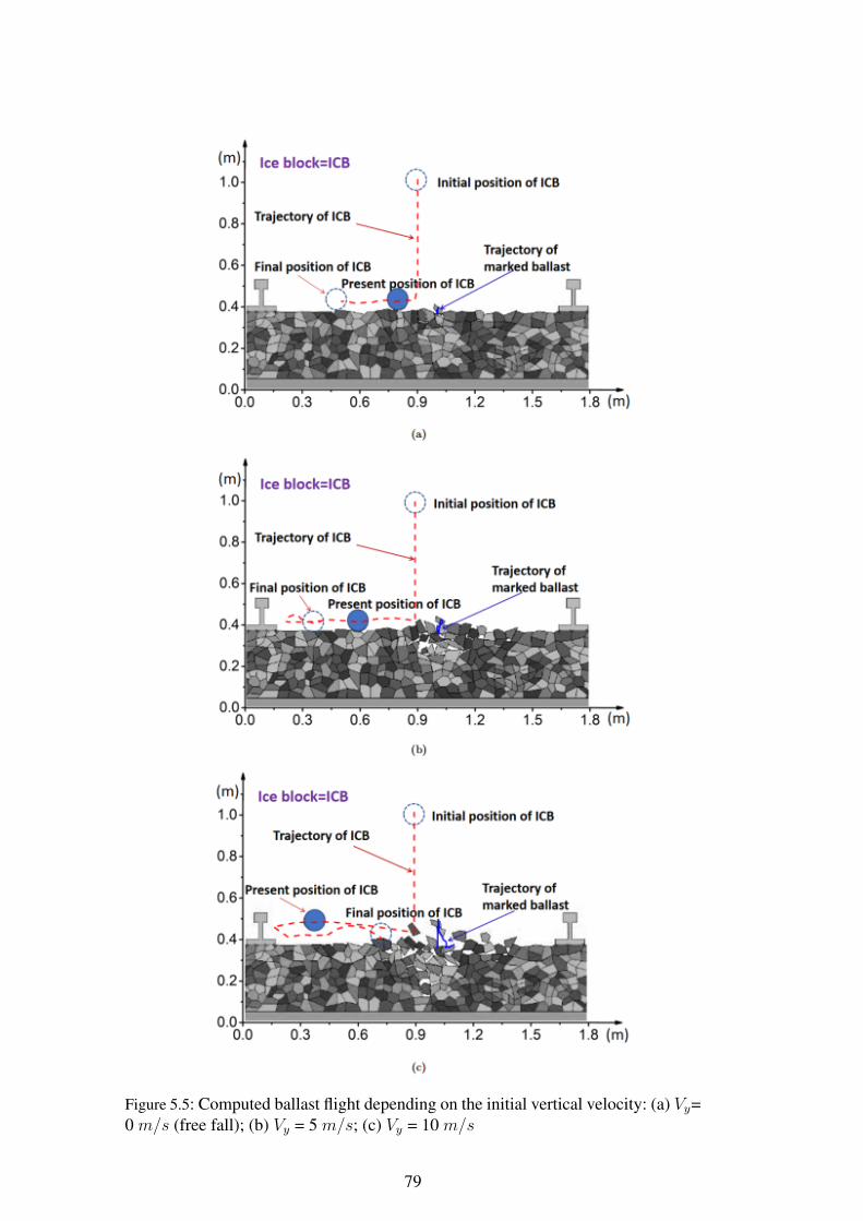
Figure 5.5: Computed ballast flight depending on the initial vertical velocity: (a) Vy=0 m/s (free fall); (b) Vy = 5 m/s; (c) Vy = 10 m/s
79
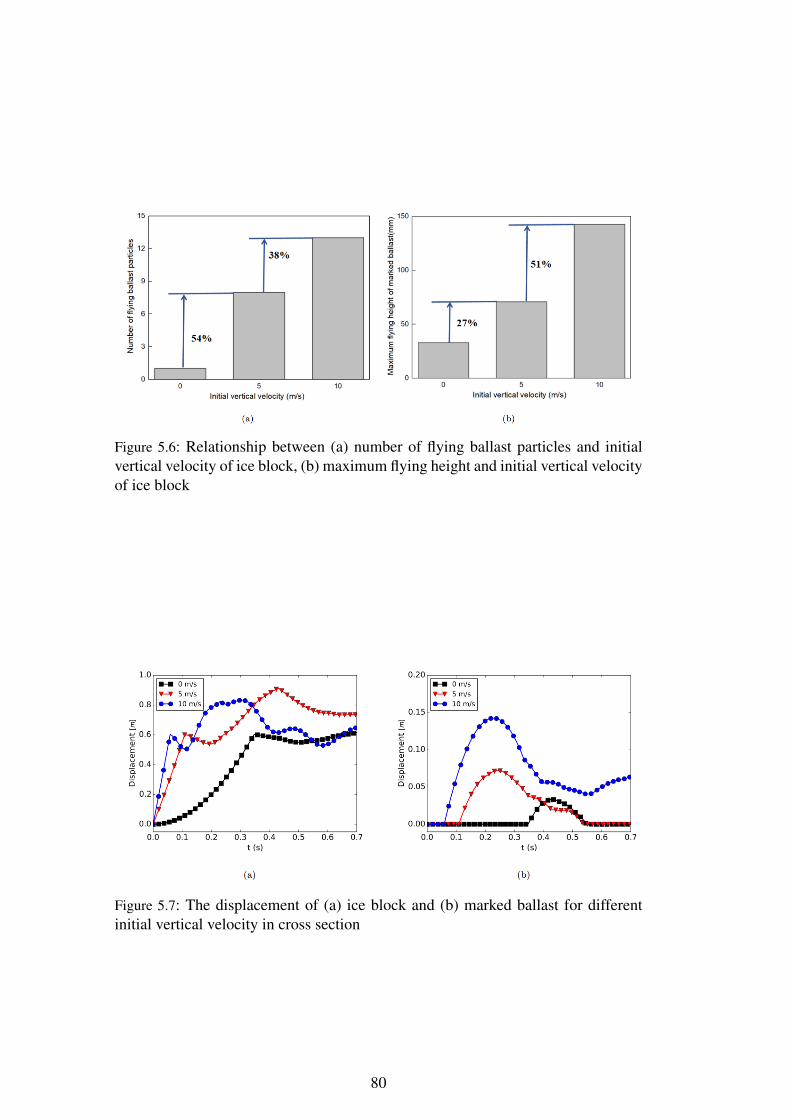
Figure 5.6: Relationship between (a) number of flying ballast particles and initialvertical velocity of ice block, (b) maximum flying height and initial vertical velocityof ice block
Figure 5.7: The displacement of (a) ice block and (b) marked ballast for differentinitial vertical velocity in cross section
80
initial collision position was set on the surface of the ballast bed. An initial verticalvelocity of 3.5 m/s which corresponded to the falling height of 600 mm, the initiallongitudinal velocity equal to the train running speed, and four initial longitudinalvelocities from 100 km/h to 400 km/h with an interval of 100 km/h were used.The trajectory of the ice block and marked ballast, as well as the phenomenon ofballast bed after the collision, is represented in Figure 5.8. It is clear that the trackbed was damaged after the collision, the ballast particles were hit and displaced, andthe surface of the track bed showed different degrees of depression. The severity ofthe damage of the track bed had a positive relationship with the initial longitudinalvelocity. For the trajectory of the ice block, the ice block quickly flew upward andforward after the collision. For the trajectory of marked ballast, we know that theballast flew to the front direction. The height and distance of the ballast flightincreased with the initial longitudinal velocity. When the dropping longitudinalvelocity is more than 300 km/h, the marked ballast may collide with the trainunderframe since the maximum height of the marked ballast after the collision ismore than 330 mm (distance from the ballast bed to train underframe)[137]. If theice and ballast particles reach the train underframe, they may accelerate significantlydue to the collision with the train or may strike off more ice /snow blocks, causingmore serious consequences. Indeed, the effects of ballast projection may vary fromdepending on where the particle lands. By considering the ballast particles flyingheight H , the impact risk is classified into three categories:
• If H ≤ 184 mm(height of UIC-60 rail), flying ballast particles have thepossibility to hit the rail;
• If 184 mm<H ≤ 330 mm, flying ballast particles have the possibility to hitthe wheels of the train ;
• If H >330 mm, flying ballast particles will certainly hit the bottom of thetrain, and probably the rail and the wheels of the train.
The displacement of the marked ballast and the ice block was calculated, as shownin Figure 5.9. Results show that the displacement of marked ballast is linear withthe increasing initial longitudinal velocity at t = 0.5 s. The displacement of markedballast of 400 km/h is about four times of that 100 km/h. Significantly, the initiallongitudinal velocity of the ice block directly affects the displacement of ice blockand ballast particles. From Figure 5.10, the numerical results show that the numberof flying ballast particles and the vertical displacement of marked ballast increasesfrom 100 km/h to 400 km/h. When the longitudinal velocity of ice block is in
81
the range of 200 km/h to 300 km/h, the results exhibit a peak of 33 % and 47% of the total number of flying ballast and a maximum flying height of markedballast. Above 300 km/h, this process evolution increases gradually until a plateauis reached. This non-uniform evolution may be related to the gradation of ballastcomposed of different particle sizes. As the longitudinal velocity increases, most ofthe small size and a part of the middle size of ballast particles in the impacted areafly above the bed surface.According to the above simulation results, the initial longitudinal velocity of thesnow / ice block which is directly dependent on the running speed of the train, hasa great impact on the ballast flight. Reducing the speed of trains is the simplestand most effective mitigation strategy. However, this method may defeat the mainpurpose of high-speed lines. The national center of operation of SNCF in Franceproposed a time schedule which divided train speed into three kinds: acceptable,tolerable and unacceptable. The weather forecast, mechanical simulation, and safetyapproach were taken into consideration.
5.4.2 Incident angle of ice block
Regarding the angle of incidence of the ice block, in the longitudinal section, thisangle can correspond to the different attachment positions of the ice, as shown inFigure 5.11. The incident angle is not an independent variable, while it is relatedto the train speed and the distance of drop as well as the ice dropping position;therefore, four angles (0o, 30o, 60o, and 90o) were investigated in the simulation.The incident angles were controlled by the velocity of the longitudinal and verticaldirections. The total velocity was set to 20 m/s.Figure 5.12 shows the trajectory of the ice block and the marked ballast as wellas the response of the track bed after the collision at different ejection angles.Based on these simulation results, it can be seen that the incident angle is alsoone of the main factors affecting ballast flight. When the incident angle is 0o, theeffect is insignificant, and just two ballast particles are moved above the surface.The maximum vertical displacement of the marked ballast is only 1.1 cm. Amongthe four angles, the ejection angle of 90o has the widest and the deepest impact,where the displacement direction of the marked ballast is essentially vertical. Whenthe angle is 30o or 60o, there is a larger longitudinal and vertical displacement.Comparing the reflection angles of the ice block in the four cases, the larger theangle of incidence, the larger angle of reflection, and the greater probability that theice block collides with the bottom of the train. Figure 5.13 shows the displacement
82
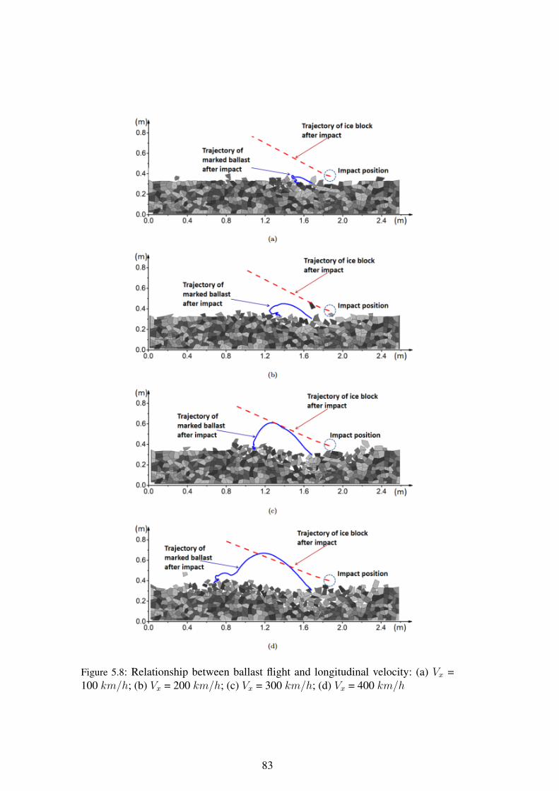
Figure 5.8: Relationship between ballast flight and longitudinal velocity: (a) Vx =100 km/h; (b) Vx = 200 km/h; (c) Vx = 300 km/h; (d) Vx = 400 km/h
83

Figure 5.9: The displacement of (a) ice block and (b) marked ballast for differentvelocities in longitudinal section
Figure 5.10: Relationship between (a) number of flying ballast particles and initiallongitudinal velocity of ice block; (b) maximum flying height and initial longitudi-nal velocity of ice block
84
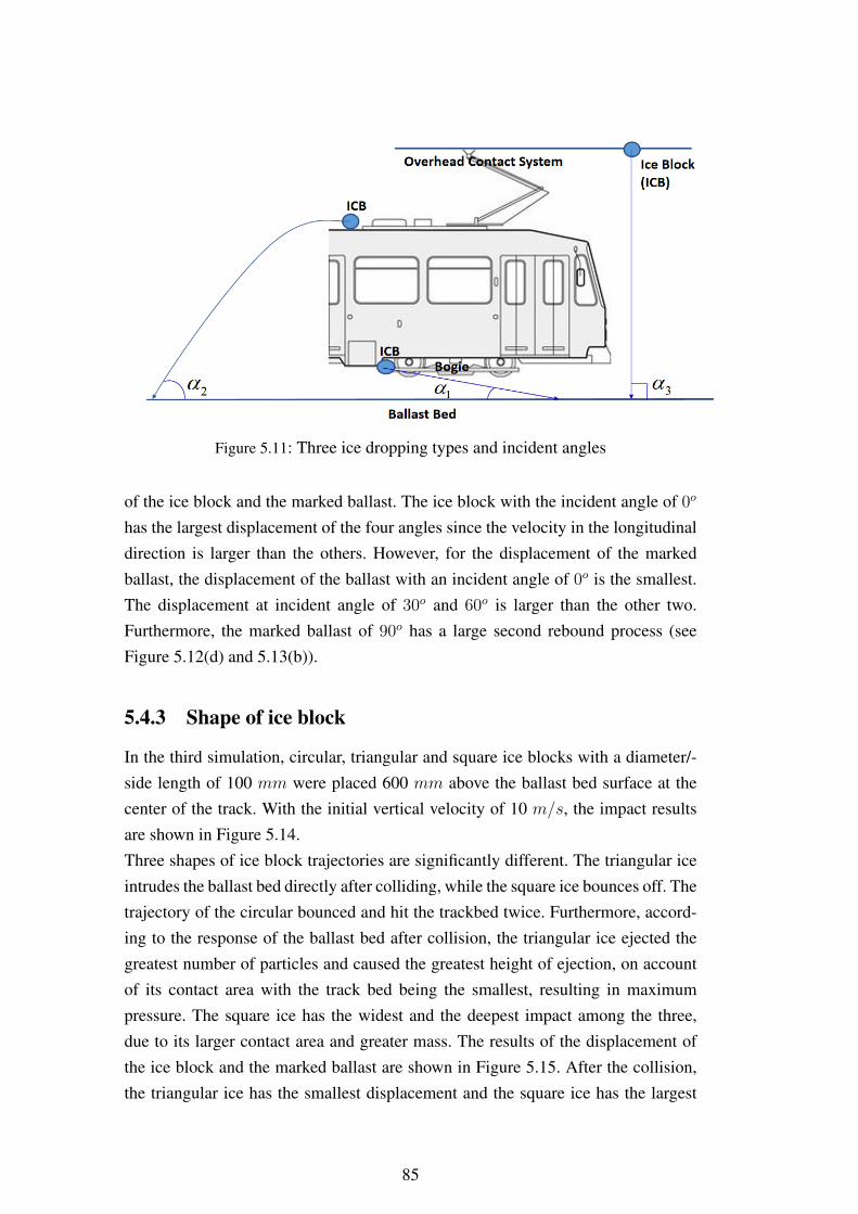
Figure 5.11: Three ice dropping types and incident angles
of the ice block and the marked ballast. The ice block with the incident angle of 0o
has the largest displacement of the four angles since the velocity in the longitudinaldirection is larger than the others. However, for the displacement of the markedballast, the displacement of the ballast with an incident angle of 0o is the smallest.The displacement at incident angle of 30o and 60o is larger than the other two.Furthermore, the marked ballast of 90o has a large second rebound process (seeFigure 5.12(d) and 5.13(b)).
5.4.3 Shape of ice block
In the third simulation, circular, triangular and square ice blocks with a diameter/-side length of 100 mm were placed 600 mm above the ballast bed surface at thecenter of the track. With the initial vertical velocity of 10 m/s, the impact resultsare shown in Figure 5.14.Three shapes of ice block trajectories are significantly different. The triangular iceintrudes the ballast bed directly after colliding, while the square ice bounces off. Thetrajectory of the circular bounced and hit the trackbed twice. Furthermore, accord-ing to the response of the ballast bed after collision, the triangular ice ejected thegreatest number of particles and caused the greatest height of ejection, on accountof its contact area with the track bed being the smallest, resulting in maximumpressure. The square ice has the widest and the deepest impact among the three,due to its larger contact area and greater mass. The results of the displacement ofthe ice block and the marked ballast are shown in Figure 5.15. After the collision,the triangular ice has the smallest displacement and the square ice has the largest
85
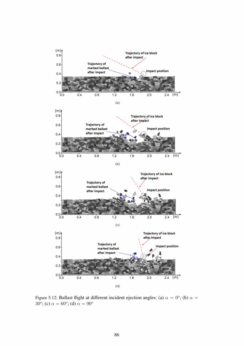
Figure 5.12: Ballast flight at different incident ejection angles: (a) α = 0o; (b) α =30o; (c) α = 60o; (d) α = 90o
86
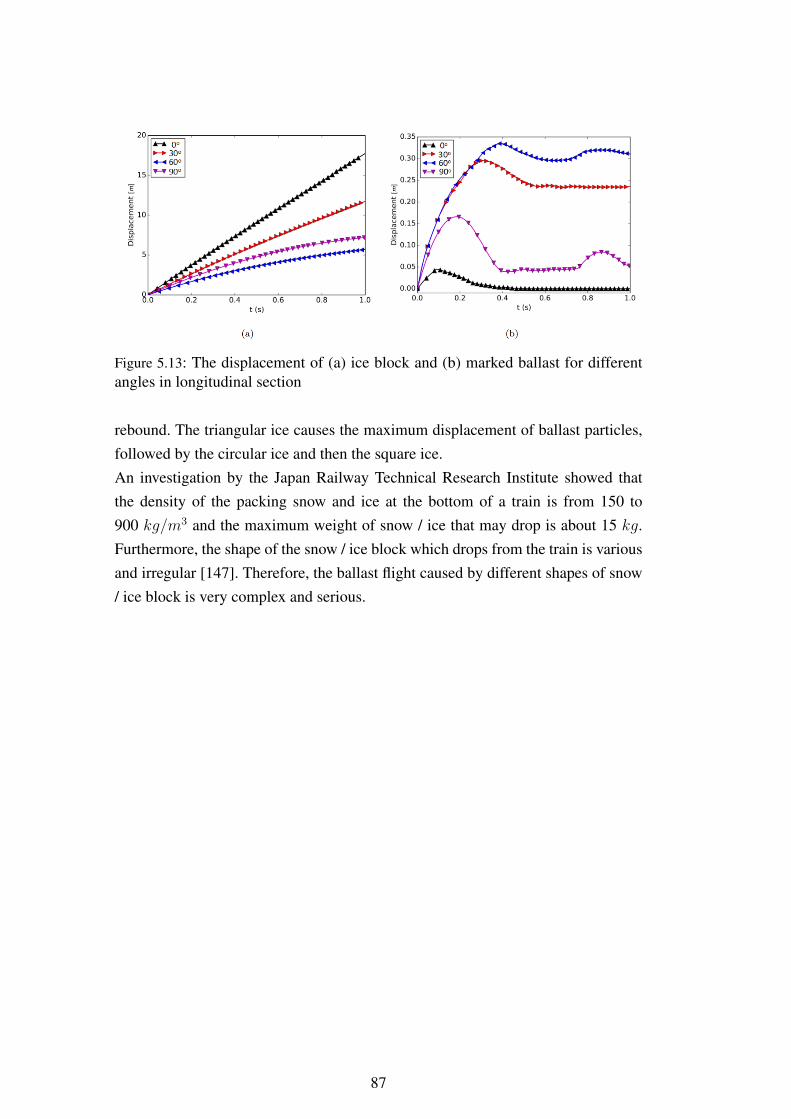
Figure 5.13: The displacement of (a) ice block and (b) marked ballast for differentangles in longitudinal section
rebound. The triangular ice causes the maximum displacement of ballast particles,followed by the circular ice and then the square ice.An investigation by the Japan Railway Technical Research Institute showed thatthe density of the packing snow and ice at the bottom of a train is from 150 to900 kg/m3 and the maximum weight of snow / ice that may drop is about 15 kg.Furthermore, the shape of the snow / ice block which drops from the train is variousand irregular [147]. Therefore, the ballast flight caused by different shapes of snow/ ice block is very complex and serious.
87
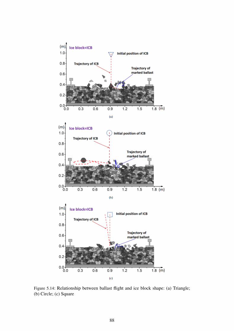
Figure 5.14: Relationship between ballast flight and ice block shape: (a) Triangle;(b) Circle; (c) Square
88
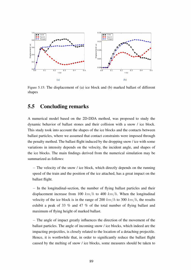
Figure 5.15: The displacement of (a) ice block and (b) marked ballast of differentshapes
5.5 Concluding remarks
A numerical model based on the 2D-DDA method, was proposed to study thedynamic behavior of ballast stones and their collision with a snow / ice block.This study took into account the shapes of the ice blocks and the contacts betweenballast particles, where we assumed that contact constraints were imposed throughthe penalty method. The ballast flight induced by the dropping snow / ice with somevariations in intensity depends on the velocity, the incident angle, and shapes ofthe ice blocks. The main findings derived from the numerical simulation may besummarized as follows:
− The velocity of the snow / ice block, which directly depends on the runningspeed of the train and the position of the ice attached, has a great impact on theballast flight.
− In the longitudinal-section, the number of flying ballast particles and theirdisplacement increase from 100 km/h to 400 km/h. When the longitudinalvelocity of the ice block is in the range of 200 km/h to 300 km/h, the resultsexhibit a peak of 33 % and 47 % of the total number of flying ballast andmaximum of flying height of marked ballast.
− The angle of impact greatly influences the direction of the movement of theballast particles. The angle of incoming snow / ice blocks, which indeed are theimpacting projectiles, is closely related to the location of a detaching projectile.Hence, it is worthwhile that, in order to significantly reduce the ballast flightcaused by the melting of snow / ice blocks, some measures should be taken to
89

prevent snow accumulating in the train and snow settlement.
− The shape of the snow / ice block affects the extent of ballast flight. Thetriangular ice block intrudes the ballast bed directly after collision, while thesquare ice bounces off. The triangular ice ejects the greatest number of particlesand causes the greatest height of ejection. The square ice has the widest and thedeepest impact among the three.
Also, it is worth noting that very little research has been done on ice block andballast particle breakage from the point of view of aerodynamic interactions andnumerical modeling . The breakage process is very important as it may indicate theviolence of the impact after the flying ballast collision step. Thus, the analysis ofthe breakage process by the DDA method is still an open problem which should beundertaken in future studies.
90
Chapter 6
Fluid-Solid coupling application tostability of breakwater
6.1 Introduction
In this chapter, a coupled Fluid-Porous-Solid model is used to study the stability ofbreakwater. The following aspects and results are emphasized:
• The porous non-linear equations are added to the inertia terms of RANS fluidequations;
• The solid model is based on the Discontinuous Deformation Analysis method;
• The coupling between the fluid and the solid is carried out by transmitting thepressure of the fluid mesh nodes to the solid polygon vertices;
• The breakwater stability depends on the thickness and slopes of the porouslayer;
• The breakwater stability depends on the shape of armour units.
6.2 Background
Breakwaters are used for the protection of harbors and beaches against wave action.Their failure may be caused by the motion of the caissons and the global instabilityof the rubble mound [148, 149]. For the motion of caissons, the most common formsare sliding, subsidence, and overturning [150], which may induce the movement ofarmour units to increase the failure of the breakwater.Elsewhere, breakwater failures have been investigated by several empirical stud-ies [151, 152] and by some numerical and experimental methods [153, 154]. Forthe computational techniques, the computational fluid dynamics (CFD) method isthe most common tool used to describe the wave impacts. Kocaman et al. [155]
91
discussed the impact of dam-break induced shock waves on a vertical wall by aCFD RANS-VOF solution. The simulation results show that the impact of dam-break flood waves on the vertical wall causes wave reflection against the wall andthe occurrence of a negative wave. The impacts of waves on the vertical wall werealso investigated by Liu et al. [156] using a two-phase compressible CFD solver.Recently, many researchers made a series of attempts to couple the fluid and solidmodels. Discrete Element Method (DEM) is usually used to calculate the movementof armour units. A wave-structure interaction method was proposed by Latham etal. [157]. In this method, the forces and the volume fraction from the CFD modelare mapped onto the DEM structure. Ren et al. [158] used a coupled SPH-DEMmethod to investigate the stability of armour units in rubble-mound breakwaters. Aninterfacial force-balance condition achieved the coupling between the fluid particle(SPH) and the solid spheres (DEM).Due to the complexity of the breakwater structure, the porous medium should alsobe considered. Traditionally, Darcy’s law and Forchheimer law were used to in-vestigate linear and non-linear structures for porous armour layer [109]. Hsu et al.[159] proposed a mathematical model based on the Volume-Averaged Reynolds-Averaged Navier-Stokes (RANS) equations that coupled the fluid and the porousmedium to describe surface wave motions in the vicinity of a coastal structure.In this model, the Forchheimer law was added by the volume-averaged process.Additionally, this fluid and porous medium coupled model is also developed inOpenFoam [110, 160, 161, 113], an extended Forchheimer law which adds a massterm that accelerates a certain amount of water considered.In this chapter, we present a triple-coupled Fluid-Porous-Solid model. The fluidmodel is described by the Volume-Averaged Reynolds-Averaged Navier-Stokes equa-tions in which the extended Forchheimer law used to calculate the porous mediumflow is added to the inertia terms [159]. The solid model, which is based on the2D-DDA, is used to compute the movement of the caisson and armour units [9].This method enables to take into account the shapes of armour units, as well asthe contact between blocks. The coupling between the fluid and the solid is carriedout by a transmission strategy of the fluid mesh nodes’ pressure towards the solidpolygon vertices, while the coupling between the fluid and the porous mediumconsists of the equations of the porous model in terms of the inertia of the fluidmodel.
92
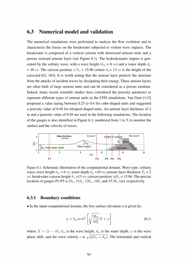
6.3 Numerical model and validation
The numerical simulations were performed to analyze the flow evolution and tocharacterize the forces on the breakwater subjected to violent wave impacts. Thebreakwater is composed of a vertical caisson with shoreward armour units and aporous seaward armour layer (see Figure 6.1). The hydrodynamic impact is gen-erated by the solitary wave, with a wave height (hw = 6 m) and a water depth dw= 10 m. The caisson position x/hc = 15.96 (where hc= 13 m is the height of thecaisson)[162, 163]. It is worth noting that the armour layer protects the structurefrom the attacks of incident waves by dissipating their energy. These armour layersare often built of large armour units and can be considered as a porous medium.Indeed, many recent scientific studies have considered the porosity parameter torepresent different types of armour units in the CFD simulations. Van Gent [112]proposed a value laying between 0.25 to 0.4 for cube-shaped units and suggesteda porosity value of 0.49 for tetrapod-shaped units. An armour layer thickness of 2m and a porosity value of 0.49 are used in the following simulations. The locationof the gauges is also identified in Figure 6.1, numbered from 1 to 5, to monitor thesurface and the velocity of waves.
Figure 6.1: Schematic illustration of the computational domain. Wave type: solitarywave; wave height hw = 6 m; water depth dw =10 m; armour layer thickness Ta = 2m; breakwater caisson height hc =13 m; caisson position: x/hc = 15.96. The preciselocation of gauges P1-P5 is 2hc, 11hc, 13hc, 14hc and 15.5hc (m), respectively.
6.3.1 Boundary conditions
• In the input computational domain, the free surface elevation η is given by:
η = hwsech2
[√3hw4d3
w
X + ψ
](6.1)
where X = (x − ct), hw is the wave height, dw is the water depth, ψ is the wavephase shift, and the wave celerity c is
√g(hw + dw). The horizontal and vertical
93
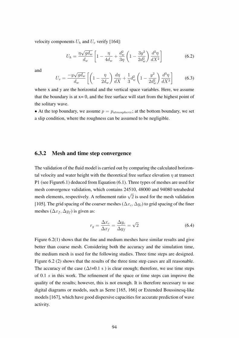
velocity components Uh and Uv verify [164]:
Uh =η√gdwdw
[1− η
4dw+d2w
3η
(1− 3y2
2d2w
)d2η
dX2
](6.2)
and
Uv =−y√gdw
dw
[(1− η
2dw
)dη
dX+
1
3d2w
(1− y2
2d2w
)d3η
dX3
](6.3)
where x and y are the horizontal and the vertical space variables. Here, we assumethat the boundary is at x= 0, and the free surface will start from the highest point ofthe solitary wave.• At the top boundary, we assume p = patmospheric; at the bottom boundary, we seta slip condition, where the roughness can be assumed to be negligible.
6.3.2 Mesh and time step convergence
The validation of the fluid model is carried out by comparing the calculated horizon-tal velocity and water height with the theoretical free surface elevation η at transectP1 (see Figure6.1) deduced from Equation (6.1). Three types of meshes are used formesh convergence validation, which contains 24510, 48000 and 94080 tetrahedralmesh elements, respectively. A refinement ratio
√2 is used for the mesh validation
[105]. The grid spacing of the coarser meshes (∆xc,∆yc) to grid spacing of the finermeshes (∆xf ,∆yf ) is given as:
rg =∆xc∆xf
=∆yc∆yf
=√
2 (6.4)
Figure 6.2(1) shows that the fine and medium meshes have similar results and givebetter than coarse mesh. Considering both the accuracy and the simulation time,the medium mesh is used for the following studies. Three time steps are designed.Figure 6.2 (2) shows that the results of the three time step cases are all reasonable.The accuracy of the case (∆t=0.1 s ) is clear enough; therefore, we use time stepsof 0.1 s in this work. The refinement of the space or time steps can improve thequality of the results; however, this is not enough. It is therefore necessary to usedigital diagrams or models, such as Serre [165, 166] or Extended Boussinesq-likemodels [167], which have good dispersive capacities for accurate prediction of waveactivity.
94
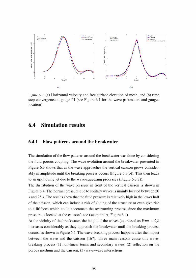
Figure 6.2: (a) Horizontal velocity and free surface elevation of mesh, and (b) timestep convergence at gauge P1 (see Figure 6.1 for the wave parameters and gaugeslocation).
6.4 Simulation results
6.4.1 Flow patterns around the breakwater
The simulation of the flow patterns around the breakwater was done by consideringthe fluid-porous coupling. The wave evolution around the breakwater presented inFigure 6.3 shows that as the wave approaches the vertical caisson grows consider-ably in amplitude until the breaking process occurs (Figure 6.3(b)). This then leadsto an up-moving jet due to the wave-squeezing processes (Figure 6.3(c)).The distribution of the wave pressure in front of the vertical caisson is shown inFigure 6.4. The normal pressure due to solitary waves is mainly located between 20s and 25 s. The results show that the fluid pressure is relatively high in the lower halfof the caisson, which can induce a risk of sliding of the structure or even give riseto a liftforce which could accentuate the overturning process since the maximumpressure is located at the caisson’s toe (see point A, Figure 6.4).At the vicinity of the breakwater, the height of the waves (expressed as H=η + dw)increases considerably as they approach the breakwater until the breaking processoccurs, as shown in Figure 6.5. The wave-breaking process happens after the impactbetween the wave and the caisson [167]. Three main reasons cause this wave-breaking process:(1) non-linear terms and secondary waves, (2) reflection on theporous medium and the caisson, (3) wave-wave interactions.
95
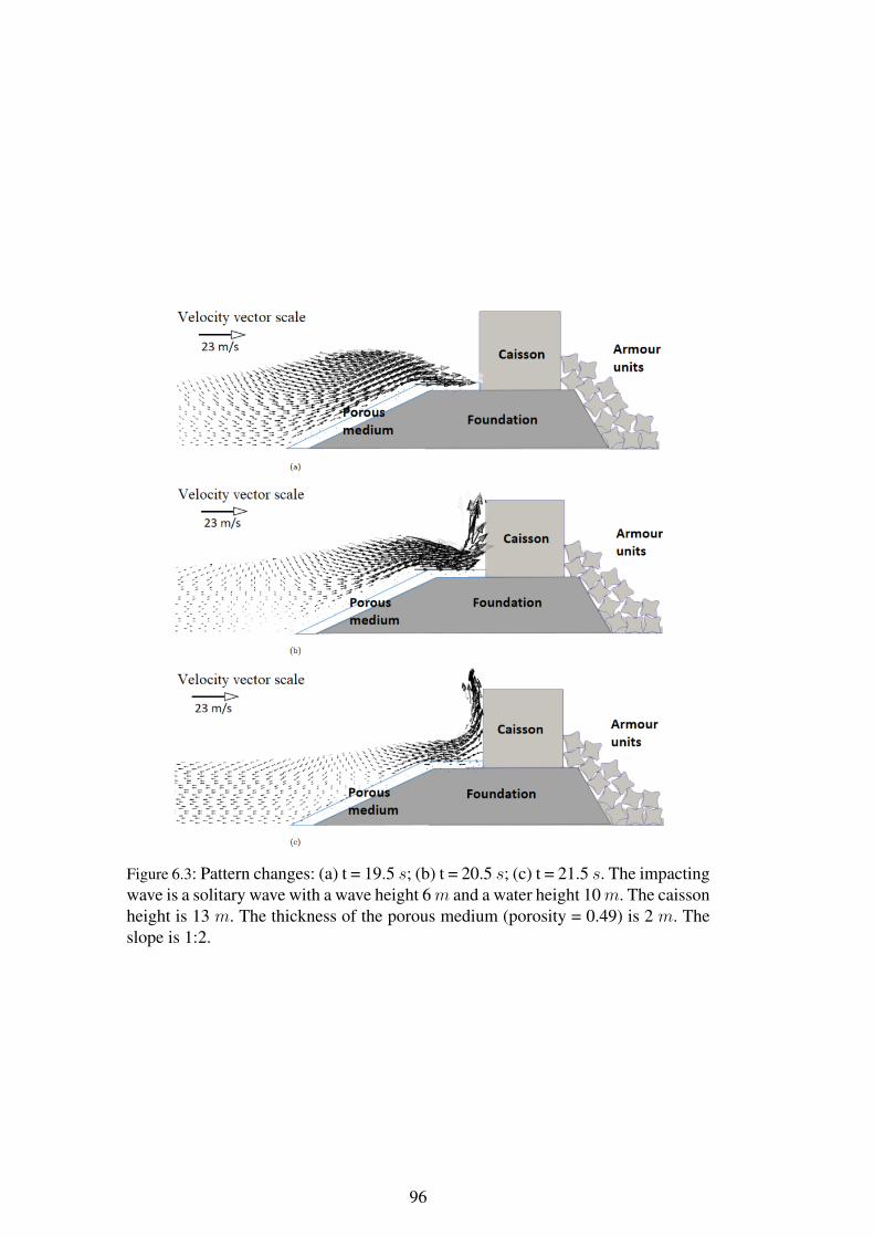
Figure 6.3: Pattern changes: (a) t = 19.5 s; (b) t = 20.5 s; (c) t = 21.5 s. The impactingwave is a solitary wave with a wave height 6m and a water height 10m. The caissonheight is 13 m. The thickness of the porous medium (porosity = 0.49) is 2 m. Theslope is 1:2.
96
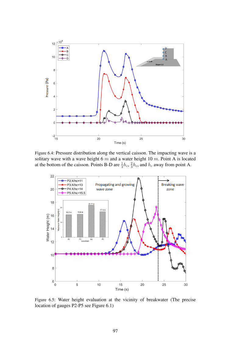
Figure 6.4: Pressure distribution along the vertical caisson. The impacting wave is asolitary wave with a wave height 6 m and a water height 10 m. Point A is locatedat the bottom of the caisson. Points B-D are 1
3hc, 2
3hc, and hc away from point A.
Figure 6.5: Water height evaluation at the vicinity of breakwater (The preciselocation of gauges P2-P5 see Figure 6.1)
97
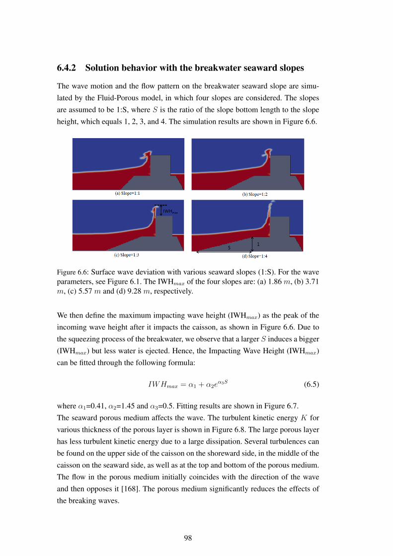
6.4.2 Solution behavior with the breakwater seaward slopes
The wave motion and the flow pattern on the breakwater seaward slope are simu-lated by the Fluid-Porous model, in which four slopes are considered. The slopesare assumed to be 1:S, where S is the ratio of the slope bottom length to the slopeheight, which equals 1, 2, 3, and 4. The simulation results are shown in Figure 6.6.
Figure 6.6: Surface wave deviation with various seaward slopes (1:S). For the waveparameters, see Figure 6.1. The IWHmax of the four slopes are: (a) 1.86 m, (b) 3.71m, (c) 5.57 m and (d) 9.28 m, respectively.
We then define the maximum impacting wave height (IWHmax) as the peak of theincoming wave height after it impacts the caisson, as shown in Figure 6.6. Due tothe squeezing process of the breakwater, we observe that a larger S induces a bigger(IWHmax) but less water is ejected. Hence, the Impacting Wave Height (IWHmax)can be fitted through the following formula:
IWHmax = α1 + α2eα3S (6.5)
where α1=0.41, α2=1.45 and α3=0.5. Fitting results are shown in Figure 6.7.The seaward porous medium affects the wave. The turbulent kinetic energy K forvarious thickness of the porous layer is shown in Figure 6.8. The large porous layerhas less turbulent kinetic energy due to a large dissipation. Several turbulences canbe found on the upper side of the caisson on the shoreward side, in the middle of thecaisson on the seaward side, as well as at the top and bottom of the porous medium.The flow in the porous medium initially coincides with the direction of the waveand then opposes it [168]. The porous medium significantly reduces the effects ofthe breaking waves.
98
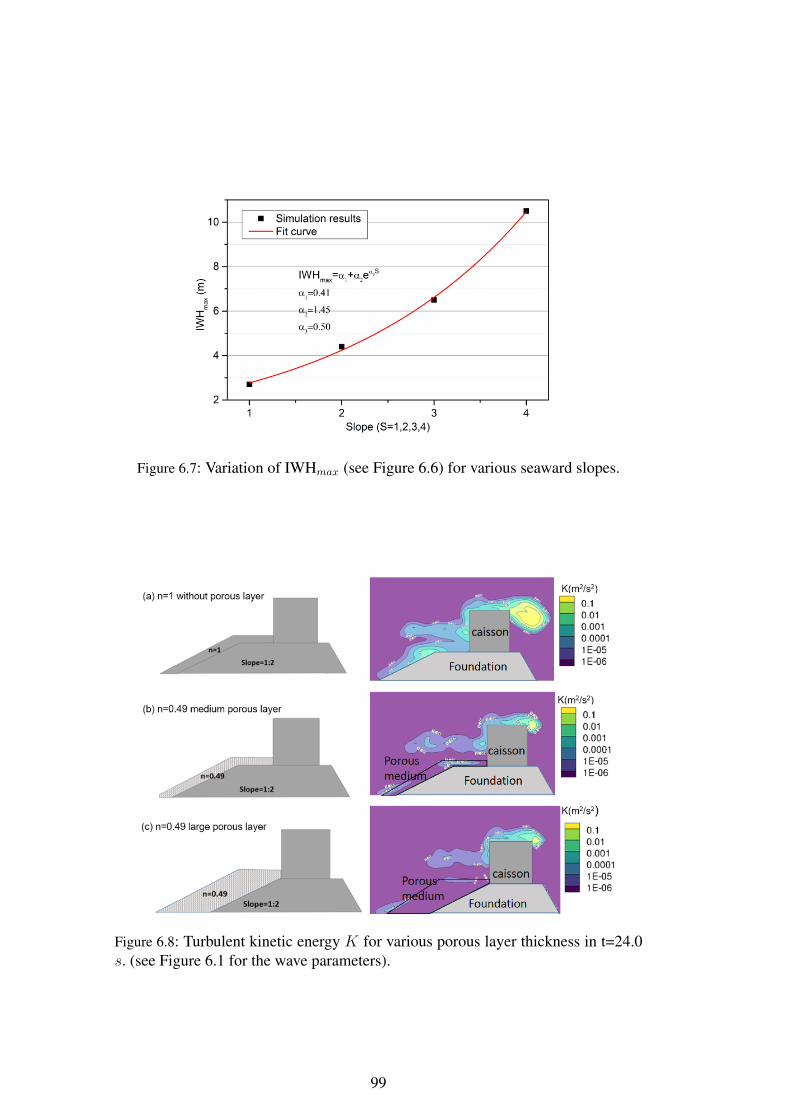
Figure 6.7: Variation of IWHmax (see Figure 6.6) for various seaward slopes.
Figure 6.8: Turbulent kinetic energy K for various porous layer thickness in t=24.0s. (see Figure 6.1 for the wave parameters).
99
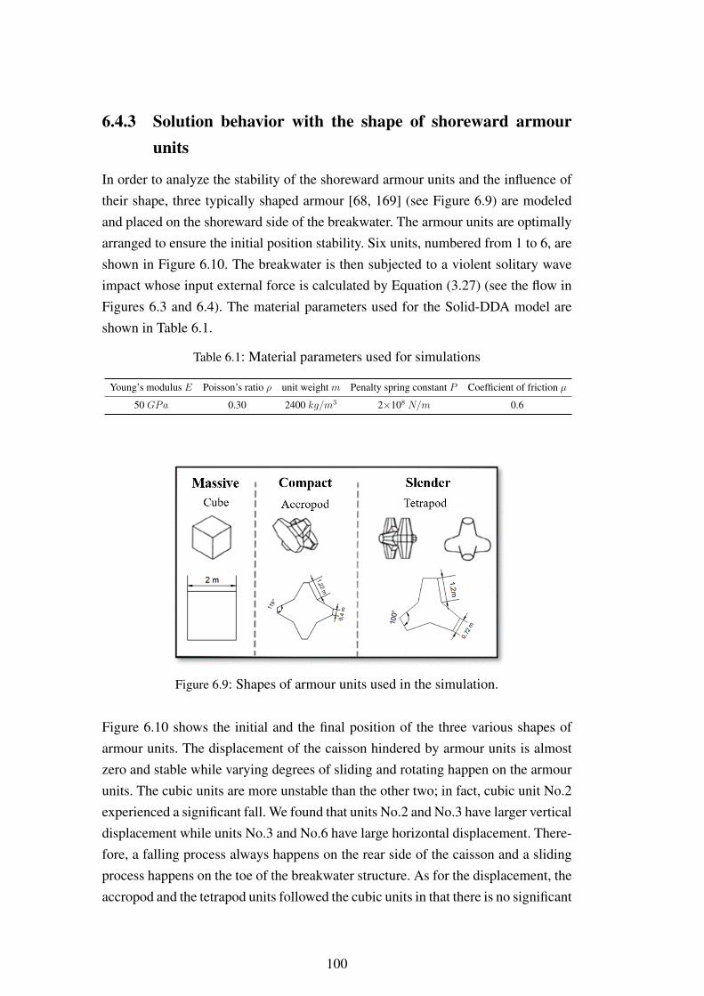
6.4.3 Solution behavior with the shape of shoreward armourunits
In order to analyze the stability of the shoreward armour units and the influence oftheir shape, three typically shaped armour [68, 169] (see Figure 6.9) are modeledand placed on the shoreward side of the breakwater. The armour units are optimallyarranged to ensure the initial position stability. Six units, numbered from 1 to 6, areshown in Figure 6.10. The breakwater is then subjected to a violent solitary waveimpact whose input external force is calculated by Equation (3.27) (see the flow inFigures 6.3 and 6.4). The material parameters used for the Solid-DDA model areshown in Table 6.1.
Table 6.1: Material parameters used for simulations
Young’s modulus E Poisson’s ratio ρ unit weight m Penalty spring constant P Coefficient of friction µ
50 GPa 0.30 2400 kg/m3 2×10⁸ N/m 0.6
Figure 6.9: Shapes of armour units used in the simulation.
Figure 6.10 shows the initial and the final position of the three various shapes ofarmour units. The displacement of the caisson hindered by armour units is almostzero and stable while varying degrees of sliding and rotating happen on the armourunits. The cubic units are more unstable than the other two; in fact, cubic unit No.2experienced a significant fall. We found that units No.2 and No.3 have larger verticaldisplacement while units No.3 and No.6 have large horizontal displacement. There-fore, a falling process always happens on the rear side of the caisson and a slidingprocess happens on the toe of the breakwater structure. As for the displacement, theaccropod and the tetrapod units followed the cubic units in that there is no significant
100
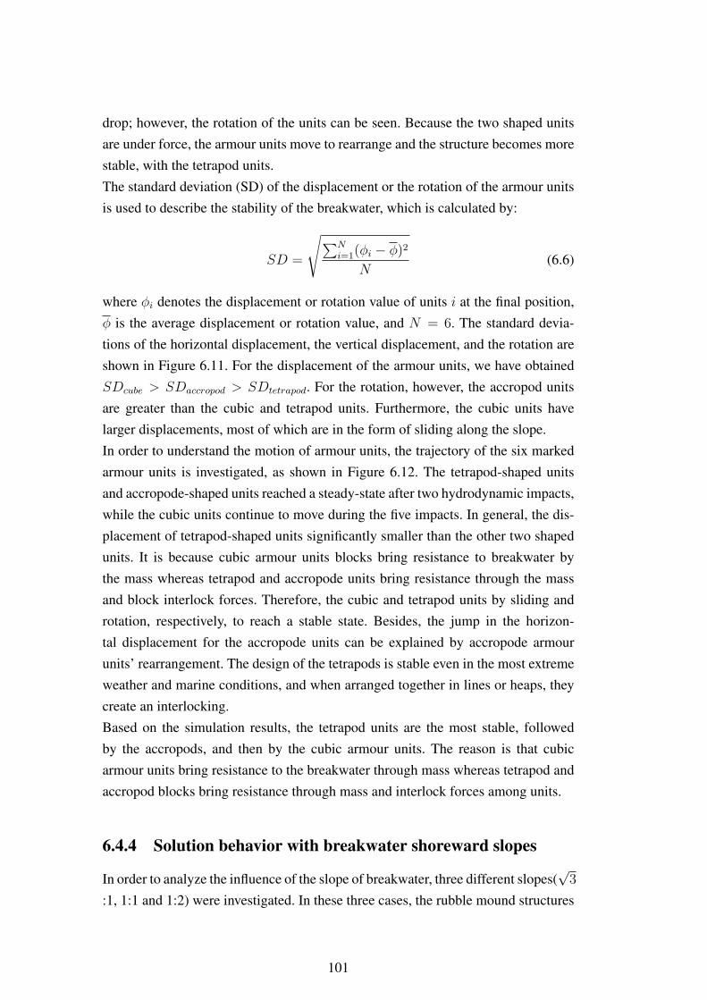
drop; however, the rotation of the units can be seen. Because the two shaped unitsare under force, the armour units move to rearrange and the structure becomes morestable, with the tetrapod units.The standard deviation (SD) of the displacement or the rotation of the armour unitsis used to describe the stability of the breakwater, which is calculated by:
SD =
√∑Ni=1(φi − φ)2
N(6.6)
where φi denotes the displacement or rotation value of units i at the final position,φ is the average displacement or rotation value, and N = 6. The standard devia-tions of the horizontal displacement, the vertical displacement, and the rotation areshown in Figure 6.11. For the displacement of the armour units, we have obtainedSDcube > SDaccropod > SDtetrapod. For the rotation, however, the accropod unitsare greater than the cubic and tetrapod units. Furthermore, the cubic units havelarger displacements, most of which are in the form of sliding along the slope.In order to understand the motion of armour units, the trajectory of the six markedarmour units is investigated, as shown in Figure 6.12. The tetrapod-shaped unitsand accropode-shaped units reached a steady-state after two hydrodynamic impacts,while the cubic units continue to move during the five impacts. In general, the dis-placement of tetrapod-shaped units significantly smaller than the other two shapedunits. It is because cubic armour units blocks bring resistance to breakwater bythe mass whereas tetrapod and accropode units bring resistance through the massand block interlock forces. Therefore, the cubic and tetrapod units by sliding androtation, respectively, to reach a stable state. Besides, the jump in the horizon-tal displacement for the accropode units can be explained by accropode armourunits’ rearrangement. The design of the tetrapods is stable even in the most extremeweather and marine conditions, and when arranged together in lines or heaps, theycreate an interlocking.Based on the simulation results, the tetrapod units are the most stable, followedby the accropods, and then by the cubic armour units. The reason is that cubicarmour units bring resistance to the breakwater through mass whereas tetrapod andaccropod blocks bring resistance through mass and interlock forces among units.
6.4.4 Solution behavior with breakwater shoreward slopes
In order to analyze the influence of the slope of breakwater, three different slopes(√
3
:1, 1:1 and 1:2) were investigated. In these three cases, the rubble mound structures
101
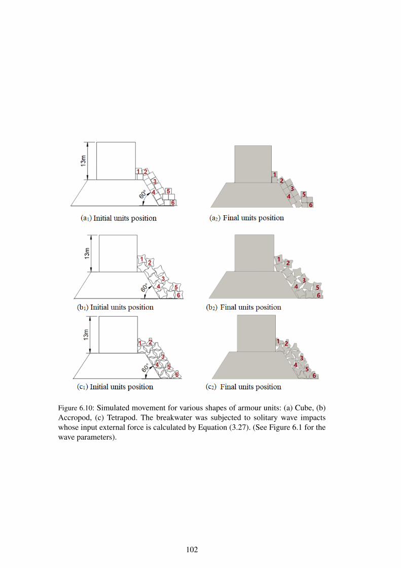
Figure 6.10: Simulated movement for various shapes of armour units: (a) Cube, (b)Accropod, (c) Tetrapod. The breakwater was subjected to solitary wave impactswhose input external force is calculated by Equation (3.27). (See Figure 6.1 for thewave parameters).
102
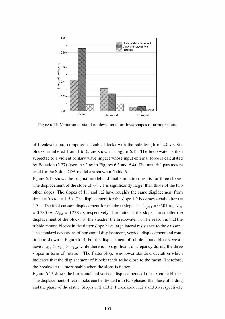
Figure 6.11: Variation of standard deviations for three shapes of armour units.
of breakwater are composed of cubic blocks with the side length of 2.0 m. Sixblocks, numbered from 1 to 6, are shown in Figure 6.13. The breakwater is thensubjected to a violent solitary wave impact whose input external force is calculatedby Equation (3.27) ((see the flow in Figures 6.3 and 6.4). The material parametersused for the Solid-DDA model are shown in Table 6.1.Figure 6.13 shows the original model and final simulation results for three slopes.The displacement of the slope of
√3 : 1 is significantly larger than those of the two
other slopes. The slopes of 1:1 and 1:2 have roughly the same displacement fromtime t = 0 s to t = 1.5 s. The displacement for the slope 1:2 becomes steady after t =1.5 s. The final caisson displacement for the three slopes is: D√3:1 = 0.501 m, D1:1
= 0.380 m, D1:2 = 0.238 m, respectively. The flatter is the slope, the smaller thedisplacement of the blocks is, the steadier the breakwater is. The reason is that therubble mound blocks in the flatter slope have large lateral resistance to the caisson.The standard deviations of horizontal displacement, vertical displacement and rota-tion are shown in Figure 6.14. For the displacement of rubble mound blocks, we allhave s√3:1 > s1:1 > s1:2, while there is no significant discrepancy during the threeslopes in term of rotation. The flatter slope was lower standard deviation whichindicates that the displacement of blocks tends to be close to the mean. Therefore,the breakwater is more stable when the slope is flatter.Figure 6.15 shows the horizontal and vertical displacements of the six cubic blocks.The displacement of rear blocks can be divided into two phases: the phase of slidingand the phase of the stable. Slopes 1: 2 and 1: 1 took about 1.2 s and 3 s respectively
103
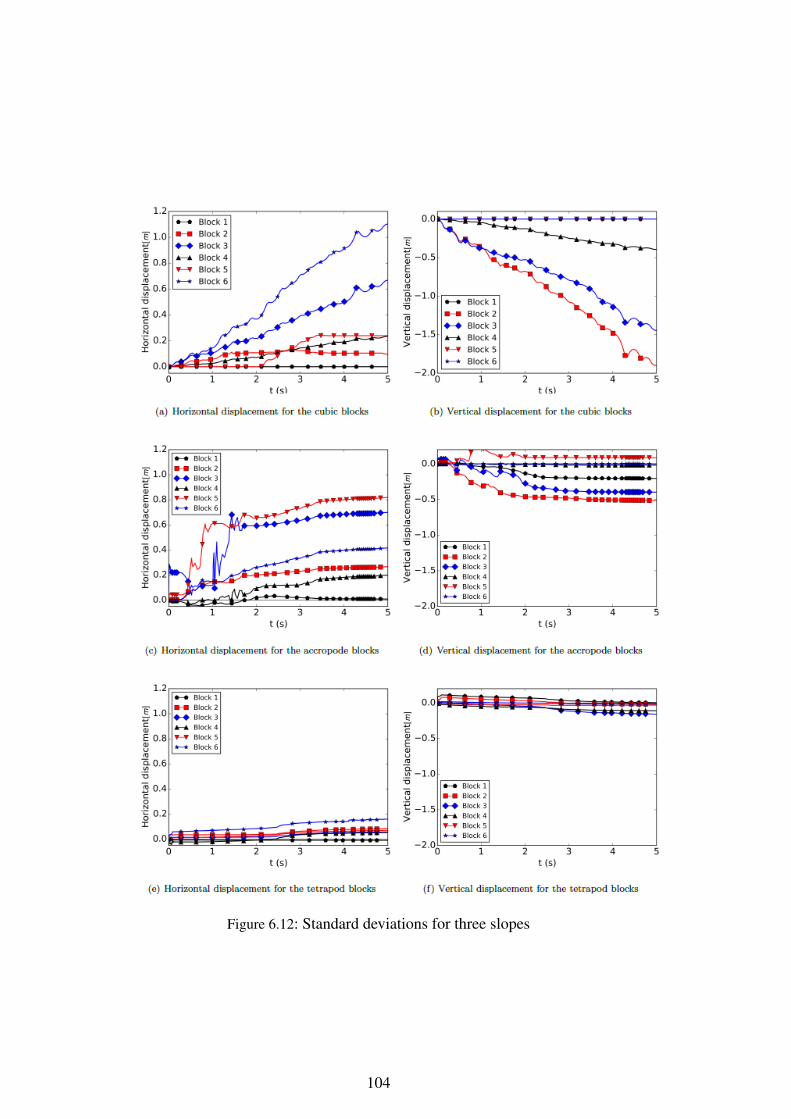
Figure 6.12: Standard deviations for three slopes
104
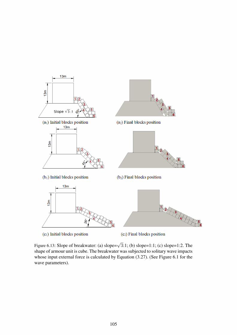
Figure 6.13: Slope of breakwater: (a) slope=√
3:1; (b) slope=1:1; (c) slope=1:2. Theshape of armour unit is cube. The breakwater was subjected to solitary wave impactswhose input external force is calculated by Equation (3.27). (See Figure 6.1 for thewave parameters).
105
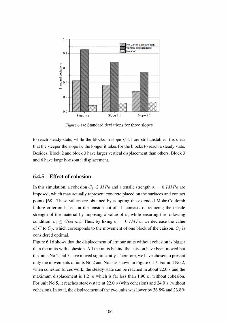
Figure 6.14: Standard deviations for three slopes
to reach steady-state, while the blocks in slope√
3:1 are still unstable. It is clearthat the steeper the slope is, the longer it takes for the blocks to reach a steady state.Besides, Block 2 and block 3 have larger vertical displacement than others. Block 3and 6 have large horizontal displacement.
6.4.5 Effect of cohesion
In this simulation, a cohesion Cf=2 MPa and a tensile strength σt = 0.7MPa areimposed, which may actually represent concrete placed on the surfaces and contactpoints [68]. These values are obtained by adopting the extended Mohr-Coulombfailure criterion based on the tension cut-off. It consists of reducing the tensilestrength of the material by imposing a value of σt while ensuring the followingcondition: σt ≤ Ccotanφ. Thus, by fixing σt = 0.7MPa, we decrease the valueof C to Cf , which corresponds to the movement of one block of the caisson. Cf isconsidered optimal.Figure 6.16 shows that the displacement of armour units without cohesion is biggerthan the units with cohesion. All the units behind the caisson have been moved butthe units No.2 and 5 have moved significantly. Therefore, we have chosen to presentonly the movements of units No.2 and No.5 as shown in Figure 6.17. For unit No.2,when cohesion forces work, the steady-state can be reached in about 22.0 s and themaximum displacement is 1.2 m which is far less than 1.90 m without cohesion.For unit No.5, it reaches steady-state at 22.0 s (with cohesion) and 24.0 s (withoutcohesion). In total, the displacement of the two units was lower by 36.8% and 23.8%
106
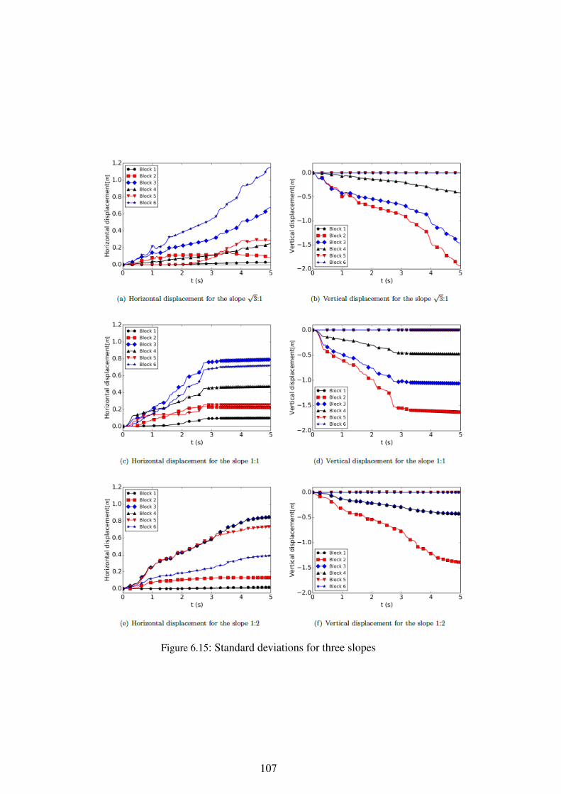
Figure 6.15: Standard deviations for three slopes
107
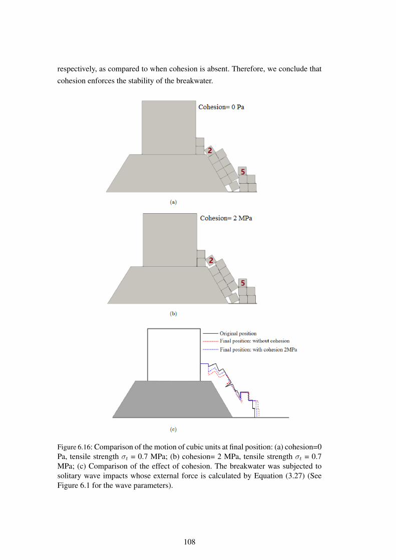
respectively, as compared to when cohesion is absent. Therefore, we conclude thatcohesion enforces the stability of the breakwater.
Figure 6.16: Comparison of the motion of cubic units at final position: (a) cohesion=0Pa, tensile strength σt = 0.7 MPa; (b) cohesion= 2 MPa, tensile strength σt = 0.7MPa; (c) Comparison of the effect of cohesion. The breakwater was subjected tosolitary wave impacts whose external force is calculated by Equation (3.27) (SeeFigure 6.1 for the wave parameters).
108
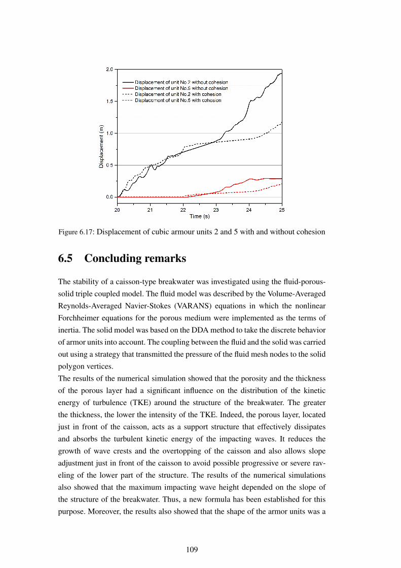
Figure 6.17: Displacement of cubic armour units 2 and 5 with and without cohesion
6.5 Concluding remarks
The stability of a caisson-type breakwater was investigated using the fluid-porous-solid triple coupled model. The fluid model was described by the Volume-AveragedReynolds-Averaged Navier-Stokes (VARANS) equations in which the nonlinearForchheimer equations for the porous medium were implemented as the terms ofinertia. The solid model was based on the DDA method to take the discrete behaviorof armor units into account. The coupling between the fluid and the solid was carriedout using a strategy that transmitted the pressure of the fluid mesh nodes to the solidpolygon vertices.The results of the numerical simulation showed that the porosity and the thicknessof the porous layer had a significant influence on the distribution of the kineticenergy of turbulence (TKE) around the structure of the breakwater. The greaterthe thickness, the lower the intensity of the TKE. Indeed, the porous layer, locatedjust in front of the caisson, acts as a support structure that effectively dissipatesand absorbs the turbulent kinetic energy of the impacting waves. It reduces thegrowth of wave crests and the overtopping of the caisson and also allows slopeadjustment just in front of the caisson to avoid possible progressive or severe rav-eling of the lower part of the structure. The results of the numerical simulationsalso showed that the maximum impacting wave height depended on the slope ofthe structure of the breakwater. Thus, a new formula has been established for thispurpose. Moreover, the results also showed that the shape of the armor units was a
109

major factor to be taken into account in the study of the stability of the structure. Inparticular, they showed that tetrapod-shaped units were the most stable, followed byacropod-shaped units and finally by cubic-shaped units, and that cohesion enforcesthe stability of the breakwater.
110
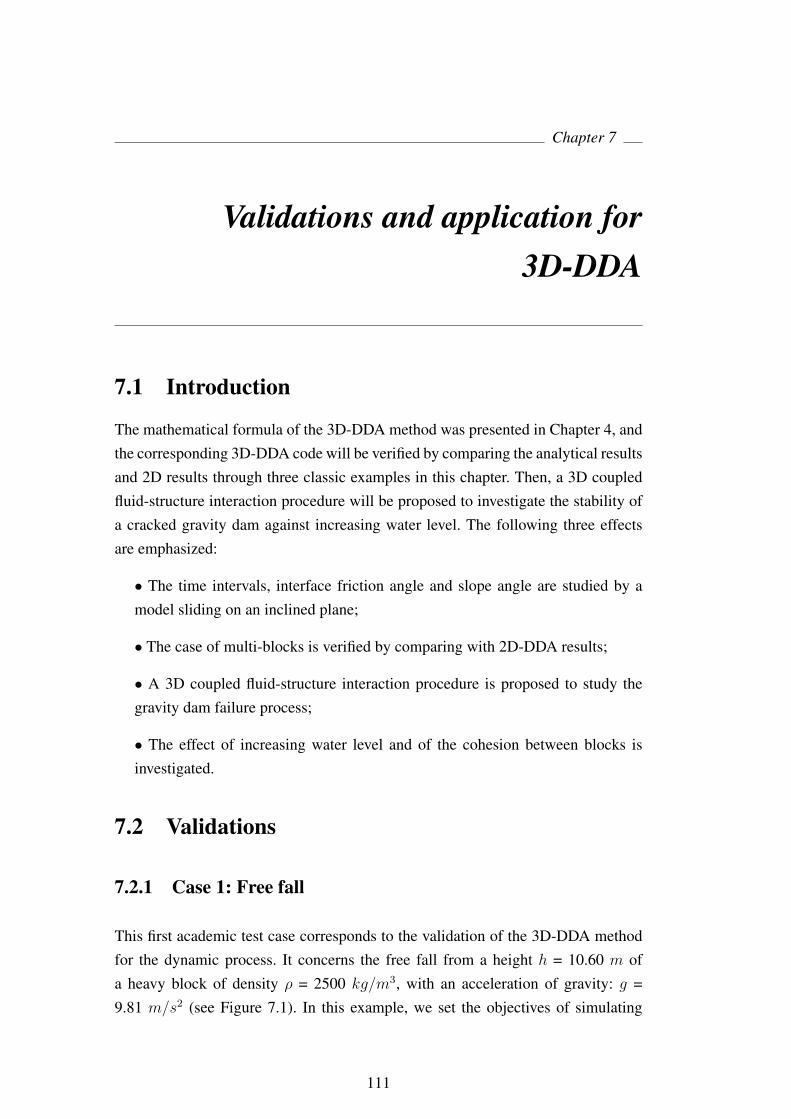
Chapter 7
Validations and application for3D-DDA
7.1 Introduction
The mathematical formula of the 3D-DDA method was presented in Chapter 4, andthe corresponding 3D-DDA code will be verified by comparing the analytical resultsand 2D results through three classic examples in this chapter. Then, a 3D coupledfluid-structure interaction procedure will be proposed to investigate the stability ofa cracked gravity dam against increasing water level. The following three effectsare emphasized:
• The time intervals, interface friction angle and slope angle are studied by amodel sliding on an inclined plane;
• The case of multi-blocks is verified by comparing with 2D-DDA results;
• A 3D coupled fluid-structure interaction procedure is proposed to study thegravity dam failure process;
• The effect of increasing water level and of the cohesion between blocks isinvestigated.
7.2 Validations
7.2.1 Case 1: Free fall
This first academic test case corresponds to the validation of the 3D-DDA methodfor the dynamic process. It concerns the free fall from a height h = 10.60 m ofa heavy block of density ρ = 2500 kg/m3, with an acceleration of gravity: g =9.81 m/s2 (see Figure 7.1). In this example, we set the objectives of simulating
111
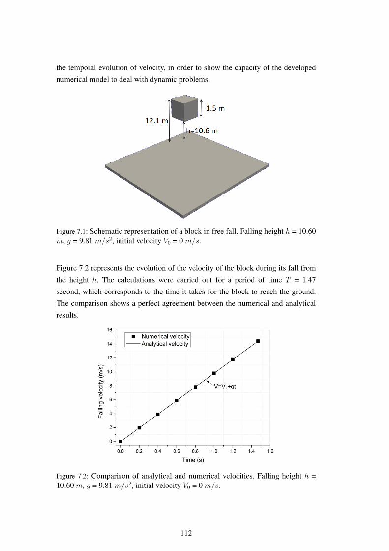
the temporal evolution of velocity, in order to show the capacity of the developednumerical model to deal with dynamic problems.
Figure 7.1: Schematic representation of a block in free fall. Falling height h = 10.60m, g = 9.81 m/s2, initial velocity V0 = 0 m/s.
Figure 7.2 represents the evolution of the velocity of the block during its fall fromthe height h. The calculations were carried out for a period of time T = 1.47second, which corresponds to the time it takes for the block to reach the ground.The comparison shows a perfect agreement between the numerical and analyticalresults.
Figure 7.2: Comparison of analytical and numerical velocities. Falling height h =10.60 m, g = 9.81 m/s2, initial velocity V0 = 0 m/s.
112

7.2.2 Case 2: Sliding on an inclined plane
A classic dynamics example is used to verify the behavior of a block on an inclinedplane [170, 171], as shown in Figure 7.3, the slope angle, the friction angle, and thetime integration are studied in this case. The model consists of two blocks, in whichthe bottom block is fixed and the upper block will accelerate and slides down onthe slope due to the gravity loading. The material constants of the two blocks are:Young’s modulus E= 3000 Pa , Poisson ratio ν= 0.25, gravity g= 9.81 m/s2, andthe normal and shear contact spring stiffness kn=ks= 50000 N/m. Under the actionof gravity, the displacement s(t) and velocity v(t) of the block are analyticallydetermined as a function of time t, given as:
s(t) = 12at2 = 1
2(g sinα− g cosα tanφ)t2
v(t) = at = (g sinα− g cosα tanφ)t(7.1)
where α is the slope angle and φ is the friction angle.
Figure 7.3: (a) Initial and (b) final positions of sliding model. α = 30o, φ=0.
Three time intervals: 0.1s, 0.01s and 0.001s are used to verify the time step conver-gence at the sliding block. Figure 7.4 shows that the results of the three-time stepcases are all reasonable. The maximum relative errors for the three time intervalsare 1.4%, 0.56%, and 0.018%, respectively. This verifies that the DDA results matchthe analytical limit equilibrium solutions at different time intervals, while smallertime steps have better accuracy.
Three cases of friction angles, 0o, 10o and 20o, are investigated in this validation.The accumulated displacements and velocities are calculated by Equation (7.1). Thevariation of the velocity and displacement for different interface friction angles are
113

Figure 7.4: Time step convergence at the sliding block. Slope angle α = 30o, frictionangle φ = 0o, time interval ∆t = 0.1s, 0.01s and 0.001s, respectively. Analyticalresults calculated by the Equation (7.1).
shown in Figure 7.6, which verifies that the DDA results show a good agreementwith the analytical solutions (see Equation (7.1)).
Figure 7.5: Variation of the (a) velocity and (b) displacement for different interfacefriction angles. Slope angle α = 30o, friction angle φ= 0o, 10o and 20o, respectively,time interval ∆t = 0.01 s. Analytical results calculated by the Equation (7.1).
.
The slope incline angles also can affect the displacement and velocity of the slidingblock by changing the acceleration along the sliding plane (see Equation (7.1)).Three different slope incline angles: α = 15o, 30o and 45o are studied. The variation
114
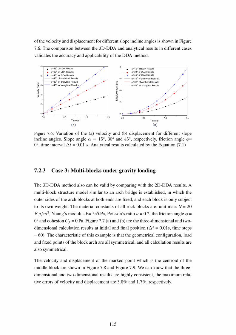
of the velocity and displacement for different slope incline angles is shown in Figure7.6. The comparison between the 3D-DDA and analytical results in different casesvalidates the accuracy and applicability of the DDA method.
Figure 7.6: Variation of the (a) velocity and (b) displacement for different slopeincline angles. Slope angle α = 15o, 30o and 45o, respectively, friction angle φ=0o, time interval ∆t = 0.01 s. Analytical results calculated by the Equation (7.1)
7.2.3 Case 3: Multi-blocks under gravity loading
The 3D-DDA method also can be valid by comparing with the 2D-DDA results. Amulti-block structure model similar to an arch bridge is established, in which theouter sides of the arch blocks at both ends are fixed, and each block is only subjectto its own weight. The material constants of all rock blocks are: unit mass M= 20Kg/m3, Young’s modulus E= 5e5 Pa, Poisson’s ratio ν = 0.2, the friction angle φ =0o and cohesionCf = 0 Pa. Figure 7.7 (a) and (b) are the three-dimensional and two-dimensional calculation results at initial and final position (∆t = 0.01s, time steps= 60). The characteristic of this example is that the geometrical configuration, loadand fixed points of the block arch are all symmetrical, and all calculation results arealso symmetrical.
The velocity and displacement of the marked point which is the centroid of themiddle block are shown in Figure 7.8 and Figure 7.9. We can know that the three-dimensional and two-dimensional results are highly consistent, the maximum rela-tive errors of velocity and displacement are 3.8% and 1.7%, respectively.
115
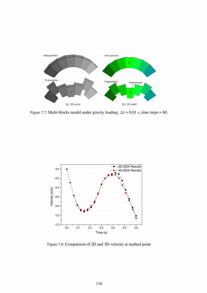
Figure 7.7: Multi-blocks model under gravity loading. ∆t = 0.01 s, time steps = 60.
Figure 7.8: Comparison of 2D and 3D velocity at marked point
116
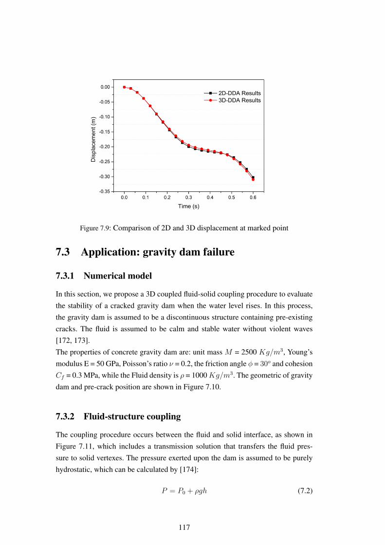
Figure 7.9: Comparison of 2D and 3D displacement at marked point
7.3 Application: gravity dam failure
7.3.1 Numerical model
In this section, we propose a 3D coupled fluid-solid coupling procedure to evaluatethe stability of a cracked gravity dam when the water level rises. In this process,the gravity dam is assumed to be a discontinuous structure containing pre-existingcracks. The fluid is assumed to be calm and stable water without violent waves[172, 173].The properties of concrete gravity dam are: unit mass M = 2500 Kg/m3, Young’smodulus E = 50 GPa, Poisson’s ratio ν = 0.2, the friction angle φ = 30o and cohesionCf = 0.3 MPa, while the Fluid density is ρ = 1000Kg/m3. The geometric of gravitydam and pre-crack position are shown in Figure 7.10.
7.3.2 Fluid-structure coupling
The coupling procedure occurs between the fluid and solid interface, as shown inFigure 7.11, which includes a transmission solution that transfers the fluid pres-sure to solid vertexes. The pressure exerted upon the dam is assumed to be purelyhydrostatic, which can be calculated by [174]:
P = P0 + ρgh (7.2)
117

Figure 7.10: Numerical model of gravity dam with pre-existing cracks
where P is the fluid pressure acting on gravity dam at water depth h above thecrack position, P0 is the fluid pressure at crack position. As the height of the waterincreases, and the corresponding pressure pi of all cells in the interface is calcu-lated. pi can then be converted into an external load applied to the boundary of thestructure. This process is repeated several times until the dam failure reached. Theforce on the cells is written as:
fi = pisi (7.3)
where pi is the fluid pressure at cell i, and si is the surface of the cell i. Finally, theglobal forces (F1, F2, F3, F4) acting on the DDA block, as shown in Figure 7.11,can be represented as:
F1 =n∑i=1
[fi(
di4di1 + di4
)ny
](
di2di1 + di2
)nz =n∑i=1
fi(di2nzdi4ny
RL)
F2 =n∑i=1
[fi(
di3di2 + di3
)ny
](
di1di2 + di3
)nz =n∑i=1
fi(di1nzdi3ny
RL)
F3 =n∑i=1
[fi(
di2di2 + di3
)ny
](
di4di3 + di4
)nz =n∑i=1
fi(di2nydi4nz
RL)
F4 =n∑i=1
[fi(
di1di1 + di4
)ny
](
di3di3 + di4
)nz =n∑i=1
fi(di1nydi3nz
RL)
(7.4)
where n is the total number of cells on the face, di1, di2, di3 and di4 are the distancefrom the given cell centroid to vertex 1, 2, 3 and 4. ny and nz represent the unitvector of y and z direction.
118
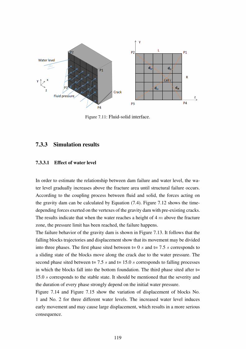
Figure 7.11: Fluid-solid interface.
7.3.3 Simulation results
7.3.3.1 Effect of water level
In order to estimate the relationship between dam failure and water level, the wa-ter level gradually increases above the fracture area until structural failure occurs.According to the coupling process between fluid and solid, the forces acting onthe gravity dam can be calculated by Equation (7.4). Figure 7.12 shows the time-depending forces exerted on the vertexes of the gravity dam with pre-existing cracks.The results indicate that when the water reaches a height of 4 m above the fracturezone, the pressure limit has been reached, the failure happens.The failure behavior of the gravity dam is shown in Figure 7.13. It follows that thefalling blocks trajectories and displacement show that its movement may be dividedinto three phases. The first phase sited between t= 0 s and t= 7.5 s corresponds toa sliding state of the blocks move along the crack due to the water pressure. Thesecond phase sited between t= 7.5 s and t= 15.0 s corresponds to falling processesin which the blocks fall into the bottom foundation. The third phase sited after t=15.0 s corresponds to the stable state. It should be mentioned that the severity andthe duration of every phase strongly depend on the initial water pressure.Figure 7.14 and Figure 7.15 show the variation of displacement of blocks No.1 and No. 2 for three different water levels. The increased water level inducesearly movement and may cause large displacement, which results in a more seriousconsequence.
119
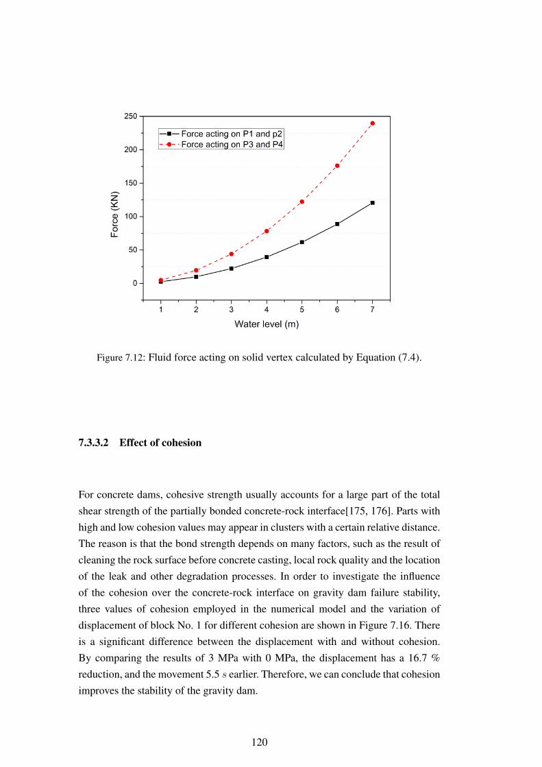
Figure 7.12: Fluid force acting on solid vertex calculated by Equation (7.4).
7.3.3.2 Effect of cohesion
For concrete dams, cohesive strength usually accounts for a large part of the totalshear strength of the partially bonded concrete-rock interface[175, 176]. Parts withhigh and low cohesion values may appear in clusters with a certain relative distance.The reason is that the bond strength depends on many factors, such as the result ofcleaning the rock surface before concrete casting, local rock quality and the locationof the leak and other degradation processes. In order to investigate the influenceof the cohesion over the concrete-rock interface on gravity dam failure stability,three values of cohesion employed in the numerical model and the variation ofdisplacement of block No. 1 for different cohesion are shown in Figure 7.16. Thereis a significant difference between the displacement with and without cohesion.By comparing the results of 3 MPa with 0 MPa, the displacement has a 16.7 %reduction, and the movement 5.5 s earlier. Therefore, we can conclude that cohesionimproves the stability of the gravity dam.
120
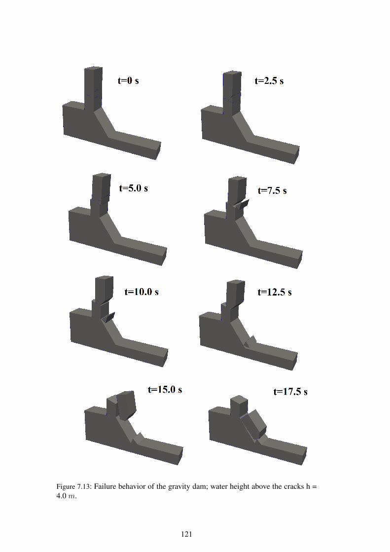
Figure 7.13: Failure behavior of the gravity dam; water height above the cracks h =4.0 m.
121
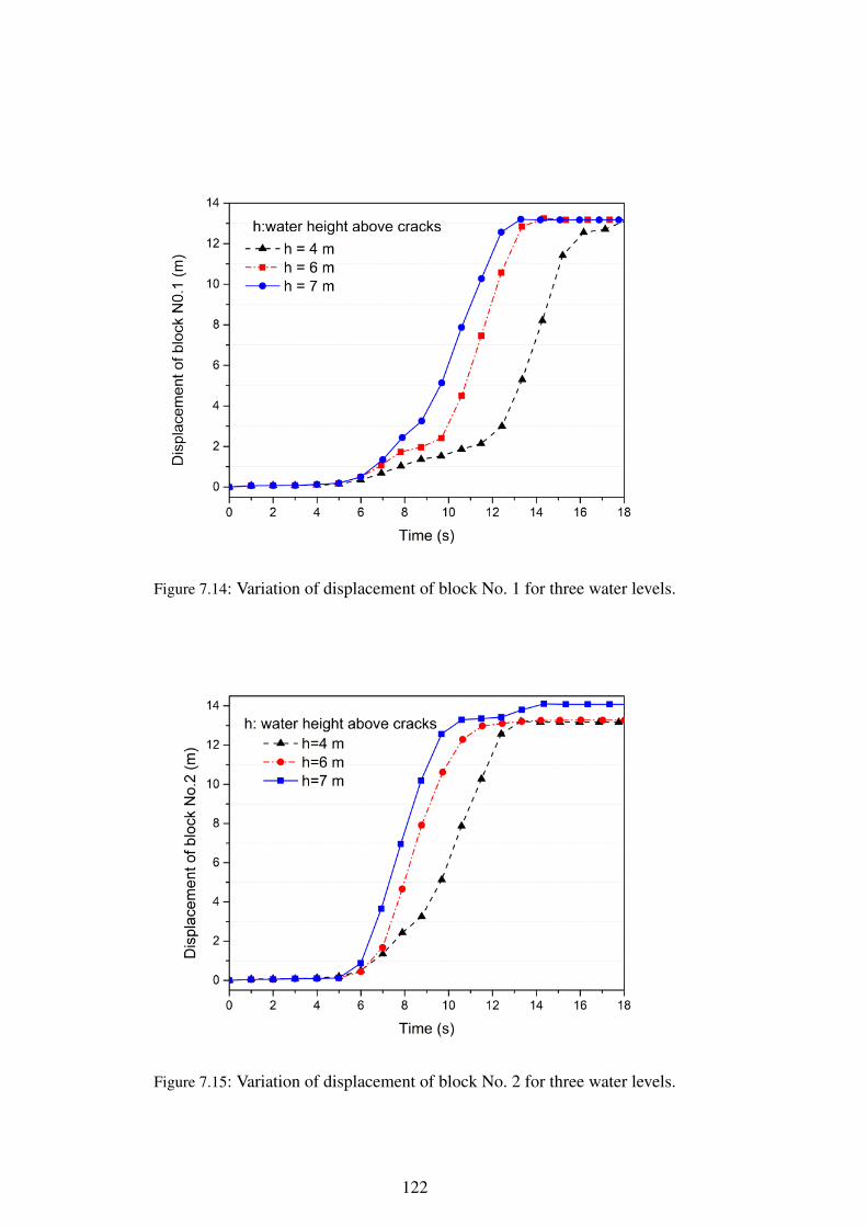
Figure 7.14: Variation of displacement of block No. 1 for three water levels.
Figure 7.15: Variation of displacement of block No. 2 for three water levels.
122
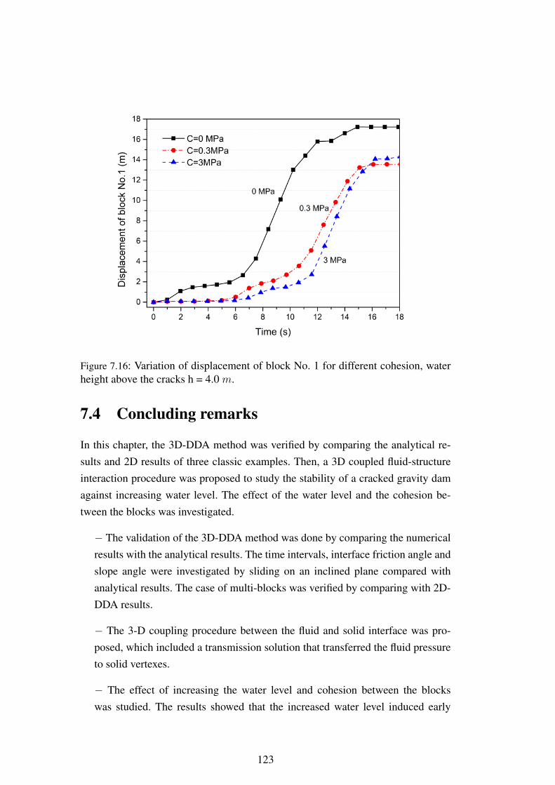
Figure 7.16: Variation of displacement of block No. 1 for different cohesion, waterheight above the cracks h = 4.0 m.
7.4 Concluding remarks
In this chapter, the 3D-DDA method was verified by comparing the analytical re-sults and 2D results of three classic examples. Then, a 3D coupled fluid-structureinteraction procedure was proposed to study the stability of a cracked gravity damagainst increasing water level. The effect of the water level and the cohesion be-tween the blocks was investigated.
− The validation of the 3D-DDA method was done by comparing the numericalresults with the analytical results. The time intervals, interface friction angle andslope angle were investigated by sliding on an inclined plane compared withanalytical results. The case of multi-blocks was verified by comparing with 2D-DDA results.
− The 3-D coupling procedure between the fluid and solid interface was pro-posed, which included a transmission solution that transferred the fluid pressureto solid vertexes.
− The effect of increasing the water level and cohesion between the blockswas studied. The results showed that the increased water level induced early
123
movement and might cause large displacement, which could result in a moreserious consequence. The cohesion improved the stability of the gravity dam.
124
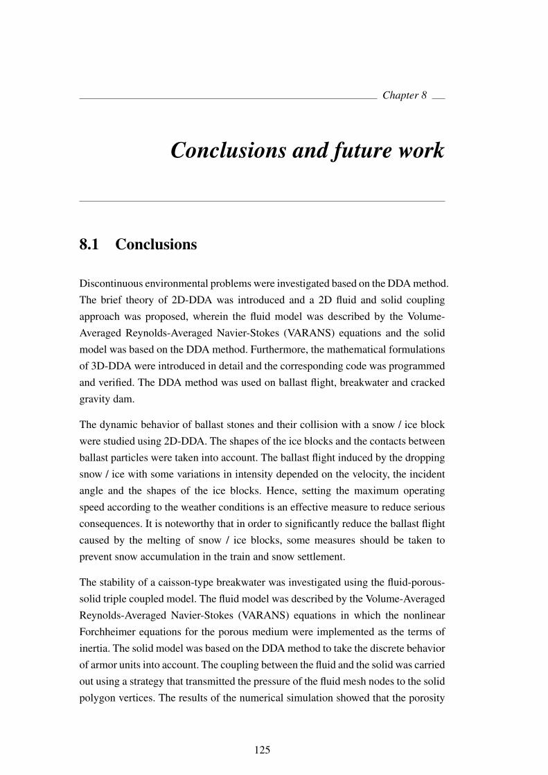
Chapter 8
Conclusions and future work
8.1 Conclusions
Discontinuous environmental problems were investigated based on the DDA method.The brief theory of 2D-DDA was introduced and a 2D fluid and solid couplingapproach was proposed, wherein the fluid model was described by the Volume-Averaged Reynolds-Averaged Navier-Stokes (VARANS) equations and the solidmodel was based on the DDA method. Furthermore, the mathematical formulationsof 3D-DDA were introduced in detail and the corresponding code was programmedand verified. The DDA method was used on ballast flight, breakwater and crackedgravity dam.
The dynamic behavior of ballast stones and their collision with a snow / ice blockwere studied using 2D-DDA. The shapes of the ice blocks and the contacts betweenballast particles were taken into account. The ballast flight induced by the droppingsnow / ice with some variations in intensity depended on the velocity, the incidentangle and the shapes of the ice blocks. Hence, setting the maximum operatingspeed according to the weather conditions is an effective measure to reduce seriousconsequences. It is noteworthy that in order to significantly reduce the ballast flightcaused by the melting of snow / ice blocks, some measures should be taken toprevent snow accumulation in the train and snow settlement.
The stability of a caisson-type breakwater was investigated using the fluid-porous-solid triple coupled model. The fluid model was described by the Volume-AveragedReynolds-Averaged Navier-Stokes (VARANS) equations in which the nonlinearForchheimer equations for the porous medium were implemented as the terms ofinertia. The solid model was based on the DDA method to take the discrete behaviorof armor units into account. The coupling between the fluid and the solid was carriedout using a strategy that transmitted the pressure of the fluid mesh nodes to the solidpolygon vertices. The results of the numerical simulation showed that the porosity
125
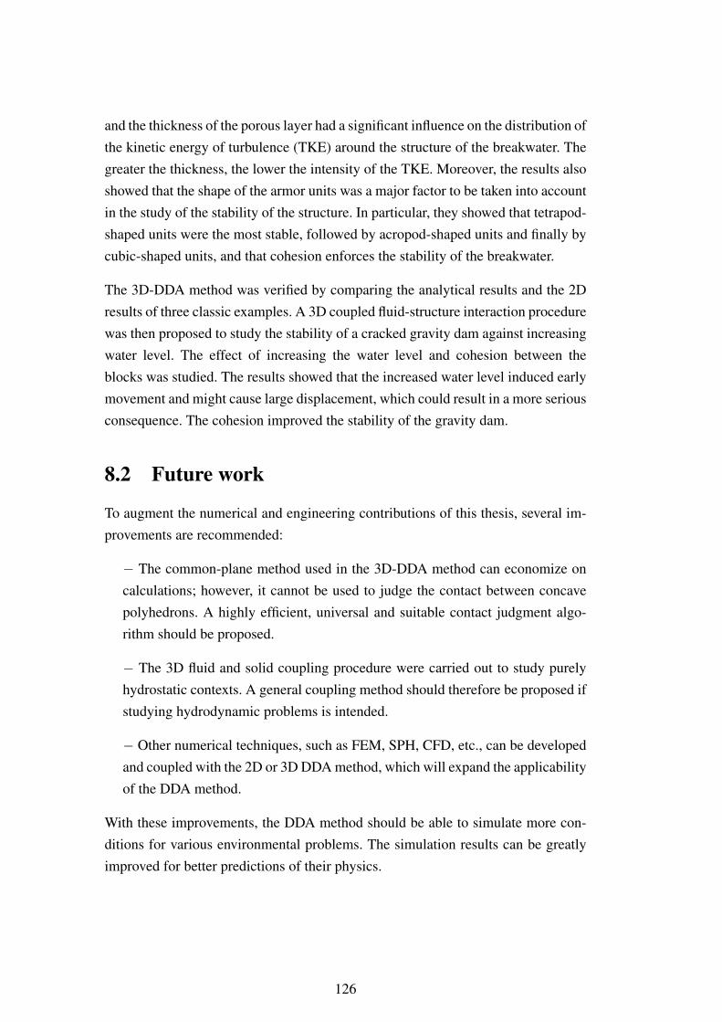
and the thickness of the porous layer had a significant influence on the distribution ofthe kinetic energy of turbulence (TKE) around the structure of the breakwater. Thegreater the thickness, the lower the intensity of the TKE. Moreover, the results alsoshowed that the shape of the armor units was a major factor to be taken into accountin the study of the stability of the structure. In particular, they showed that tetrapod-shaped units were the most stable, followed by acropod-shaped units and finally bycubic-shaped units, and that cohesion enforces the stability of the breakwater.
The 3D-DDA method was verified by comparing the analytical results and the 2Dresults of three classic examples. A 3D coupled fluid-structure interaction procedurewas then proposed to study the stability of a cracked gravity dam against increasingwater level. The effect of increasing the water level and cohesion between theblocks was studied. The results showed that the increased water level induced earlymovement and might cause large displacement, which could result in a more seriousconsequence. The cohesion improved the stability of the gravity dam.
8.2 Future work
To augment the numerical and engineering contributions of this thesis, several im-provements are recommended:
− The common-plane method used in the 3D-DDA method can economize oncalculations; however, it cannot be used to judge the contact between concavepolyhedrons. A highly efficient, universal and suitable contact judgment algo-rithm should be proposed.
− The 3D fluid and solid coupling procedure were carried out to study purelyhydrostatic contexts. A general coupling method should therefore be proposed ifstudying hydrodynamic problems is intended.
− Other numerical techniques, such as FEM, SPH, CFD, etc., can be developedand coupled with the 2D or 3D DDA method, which will expand the applicabilityof the DDA method.
With these improvements, the DDA method should be able to simulate more con-ditions for various environmental problems. The simulation results can be greatlyimproved for better predictions of their physics.
126
Bibliography
[1] JA Hudson. Engineering Rock Mechanics: Part 2: Illustrative Worked
Examples. Elsevier, 2001.
[2] MS Khan. Investigation of discontinuous deformation analysis for applica-
tion in jointed rock masses. PhD thesis, Department of Civil EngineeringUniversity of Toronto, 2010.
[3] RE Goodman, RL Taylor, and TL Brekke. A model for the mechanics ofjointed rock. Journal of Soil Mechanics & Foundations Div, 14(3):637–659,1968.
[4] BC Burman. Development of a numerical model for discontinua. Australian
Geomechanics Journal, 4(1):13–22, 1974.
[5] V Sarhosis, K Bagi, J Lemos, and G Milani. Computational modeling of
masonry structures using the discrete element method. IGI Global, 2016.
[6] Y Jiao, X Zhang, H Zhang, H Li, S Yang, and J Li. A coupled thermo-mechanical discontinuum model for simulating rock cracking induced bytemperature stresses. Computers and Geotechnics, 67:142–149, 2015.
[7] G Huang, P Kulatilake, S Shreedharan, and S Cai. 3-D discontinuum nu-merical modeling of subsidence incorporating ore extraction and backfillingoperations in an underground iron mine in China. International Journal of
Mining Science and Technology, 27(2):191–201, 2017.
[8] PA Cundall. A computer model for simulating progressive, large-scalemovement in blocky rock system. In Proceedings of the International
Symposium on Rock Mechanics, 1971, pages 1–8, 1971.
[9] G-H Shi. Discontinuous deformation analysis: a new numerical modelfor the statics and dynamics of deformable block structures. Engineering
computations, 9(2):157–168, 1992.
[10] Y H Hatzor, G Ma, and G-h Shi. Discontinuous Deformation Analysis in
Rock Mechanics Practice. CRC Press, 2017.
127
[11] YH Hatzor, AA Arzi, and M Tsesarsky. Realistic dynamic analysis of jointedrock slopes using DDA. In Proceedings of 5th International Conference on
Analysis of Discontinuous Deformation, 2002.
[12] DM Doolin and Nicholas Sitar. Time integration in discontinuous deforma-tion analysis. Journal of engineering mechanics, 130(3):249–258, 2004.
[13] PA Cundall. Distinct element models of rock and soil structure. Analytical
and computational methods in engineering rock mechanics, pages 129–163,1987.
[14] MM MacLaughlin and DM Doolin. Review of validation of the discon-tinuous deformation analysis (DDA) method. International journal for
numerical and analytical methods in geomechanics, 30(4):271–305, 2006.
[15] X Dong and WU AQ. A preliminary application of discontinuous deforma-tion analysis (DDA) to the three gorges project on Yangtze River, China. InProceedings of the first international forum on discontinuous deformation
analysis (DDA) and simulations of discontinuous media, Berkeley, USA,pages 310–317, 1996.
[16] MM MacLaughlin and RD Langston. Discrete element analysis of a minestope in blocky rock: a comparison study of DDA and UDEC. In Proceed-
ings of the Fourth International Conference on Analysis of Discontinuous
Deformation, pages 111–120. University of Glasgow Glasgow, 2001.
[17] G Yagoda-Biran. Seismic Hazard Analysis Using the Numerical DDA
Method. PhD thesis, Ben-Gurion University of the Negev, 2013.
[18] G Yagoda-Biran and YH Hatzor. Benchmarking the numerical discontinuousdeformation analysis method. Computers and Geotechnics, 71:30–46, 2016.
[19] A McBride and F Scheele. Investigation of discontinuous deformationanalysis using physical laboratory models. In Proc. Fourth International
Conference on Discontinuous Deformation Analysis, pages 73–82, 2001.
[20] P Cundall, M Voegele, C Fairhurst, et al. Computerized design of rockslopes using interactive graphics for the input and output of geometrical data.In The 16th US Symposium on Rock Mechanics (USRMS). American RockMechanics Association, 1975.
[21] T Ishikawa, Y Ohnishi, and A Namura. DDA applied to deformation analysisof coarse granular materials (ballast). Proc. 2nd Int. Conf. on Analysis
of Discontinuous Deformation. Japan Institute of Systems Research: Kyoto,
128
Japan, pages 253–262, 1997.
[22] D Ding, A Ouahsine, W Xiao, and P Du. Numerical study of ballast-flight caused by dropping snow/ice blocks in high-speed railways usingDiscontinuous Deformation Analysis (DDA). Transportation Geotechnics,22:100314, 2020.
[23] DM Doolin and N Sitar. Displacement accuracy of discontinuous defor-mation analysis method applied to sliding block. Journal of engineering
mechanics, 128(11):1158–1168, 2002.
[24] M MacLaughlin, N Sitar, D Doolin, and T Abbot. Investigation of slope-stability kinematics using discontinuous deformation analysis. International
journal of rock mechanics and mining sciences, 38(5):753–762, 2001.
[25] MM MacLaughlin, N Sitar, et al. Kinematics of sliding on a hinged failuresurface. In Proceedings of 2nd North American Rock Mechanics Symposium.American Rock Mechanics Association, 1996.
[26] O Yuzo, Chen G, and Miki S. Recent development of DDA in rock mechanicspractice. In The First International Conference on Analysis of Discontinuous
Deformation, pages 26–47, Changli, Taiwan, 1995.
[27] TC Ke. The issue of rigid body rotation in DDA. In Proceedings of
first international forum on discontinuous deformation analysis (DDA) and
simulations of discontinuous media, pages 18–25. Berkeley, 1996.
[28] CY Koo, JC Chern, and S Chen. Development of second order displacementfunction for DDA. In Proceedings of the first international conference
on analysis of discontinuous deformation. National Central University:
Chungli, Taiwan ROC, pages 91–108, 1995.
[29] TC Ke. Application of DDA to simulate fracture propagation in solid.In Proceedings of the Second International Conference on Analysis of
Discontinuous Deformation, Kyoto, Japan, pages 9–12, 1997.
[30] DM Doolin and N Sitar. Accuracy of the DDA method for frictionless impact.In Mining and Tunnelling Innovation and Opportunity, North American Rock
Mechanics Symposium-Tunneling Association of Canada, pages 1289–1296,2002.
[31] K Shyu, X Wang, and CT Chang. Dynamic behaviors in discontinuous elasticmedia using DDA. In Proceedings of the Third International Conference on
Analysis of Discontinuous Deformation from Theory to Practice, pages 243–
129
252, 1999.
[32] D Stewart. Time-stepping methods and the mathematics of rigid bodydynamics. Impact and Friction of Solids, Structures and Machines, 1, 2000.
[33] R Kamai. Estimation of historical seismic ground-motions using back
analysis of structural failures in archaeological sites. Ben-Gurion Universityof the Negev, 2006.
[34] S Kaidi, A Ouahsine, P Sergent, and M Rouainia. Analyse des deformationsdiscontinues pour l’evaluation de la stabilite des digues en enrochements souschargement sismique. Comptes Rendus Mecanique, 340(10):731–738, 2012.
[35] CY Wang, CC Chuang, and Jopan Sheng. Time integration theories forthe DDA method with finite element meshes. In Proceedings of 1st Int.
Forum on Discontinuous Deformation Analysis (DDA) and Simulations of
Discontinuous Media, pages 263–287. New Mexico,USA, 1996.
[36] P Komodromos, L Papaloizou, and P Polycarpou. Simulation of the responseof ancient columns under harmonic and earthquake excitations. Engineering
Structures, 30(8):2154–2164, 2008.
[37] MM MacLaughlin and KK Clapp. Discrete element analysis of an under-ground opening in blocky rock: an investigation of the differences betweenUDEC and DDA results. In Discrete Element Methods: Numerical Modeling
of Discontinua, pages 329–334. 2002.
[38] AT McBride and F Scheele. Validation of discontinuous deformationanalysis using a physical model. Structural Engineering, Mechanics and
Computation, pages 719–726, 2001.
[39] K Irie, T Koyama, S Nishiyama, Y Yasuda, and Y Ohnishi. A numericalstudy on the effect of shear resistance on the landslide by discontinuousdeformation analysis (DDA). Geomechanics and Geoengineering, 7(1):57–68, 2012.
[40] MM MacLaughlin and N Sitar. Rigid body rotations in DDA. In Proceedings
of the first international forum on discontinuous deformation analysis (DDA)
and simulation of discontinuous media, Berkeley, pages 620–635, 1996.
[41] YM Cheng and YH Zhang. Rigid body rotation and block internal discretiza-tion in DDA analysis. International Journal for Numerical and Analytical
Methods in Geomechanics, 24(6):567–578, 2000.
130
[42] CY Koo and Jin-Ching Chern. Modification of the DDA method for rigidblock problems. International Journal of Rock Mechanics and Mining
Sciences, 35(6):683–693, 1998.
[43] CY Koo and JC Chern. The development of dda with third order displace-ment function. In Proceedings of the First International Forum on Discontin-
uous Deformation Analysis (DDA) and Simulations of Discontinuous Media,pages 12–14. Berkeley, CA. TSI Press: Albuquerque, 1996.
[44] Max Y Ma, M Zaman, and JH Zhou. Discontinuous deformation analysisusing the third order displacement function. In Proceedings of the First
International Forum on Discontinuous Deformation Analysis (DDA) and
Simulations of Discontinuous Media, pages 383–394. Berkeley, CA. TSIPress: Albuquerque, 1996.
[45] SM Hsiung. Discontinuous deformation analysis (DDA) with nth order poly-nomial displacement functions. In DC Rocks 2001, The 38th US Symposium
on Rock Mechanics (USRMS). American Rock Mechanics Association, 2001.
[46] XB Wang, XL Ding, B Lu, and A Wu. DDA with higher order polynomialdisplacement functions for large elastic deformation problems. In Proceed-
ings of the 8th International Conference on the analysis of discontinuous
deformation, Beijing, China, pages 89–94, 2007.
[47] TC Ke and J Bray. Modeling of particulate media using discontinuousdeformation analysis. Journal of engineering mechanics, 121(11):1234–1243, 1995.
[48] P Wriggers and G Zavarise. Computational contact mechanics. Encyclopedia
of computational mechanics, 2004.
[49] P Papadopoulos and JM Solberg. A lagrange multiplier method for thefinite element solution of frictionless contact problems. Mathematical and
computer modelling, 28(4-8):373–384, 1998.
[50] T Belytschko and M Neal. Contact-impact by the pinball algorithm withpenalty and lagrangian methods. International Journal for Numerical
Methods in Engineering, 31(3):547–572, 1991.
[51] B Amadei. Recent extensions to the DDA method. In Proc. of first Int. Forum
on Discontinuous Deformation Analysis (DDA), Berkley, California, 1996.
[52] CT Lin, B Amadei, J Jung, and J Dwyer. Extensions of discontinuousdeformation analysis for jointed rock masses. International Journal of Rock
131
Mechanics and Mining Sciences, 33(7):671–694, 1996.
[53] BK Kannan and Steven N Kramer. An augmented lagrange multiplier basedmethod for mixed integer discrete continuous optimization and its applica-tions to mechanical design. Journal of mechanical design, 116(2):405–411,1994.
[54] V Sarhosis, JV Lemos, and K Bagi. Discrete element modeling. In Numerical
Modeling of Masonry and Historical Structures, pages 469–501. Elsevier,2019.
[55] J Eliáš. Simulation of railway ballast using crushable polyhedral particles.Powder Technology, 264:458–465, 2014.
[56] M Hazay and A Munjiza. Introduction to the combined finite-discreteelement method. In Computational Modeling of Masonry Structures Using
the Discrete Element Method, pages 123–145. IGI Global, 2016.
[57] Y Ohnishi, S Nishiyama, S Akao, M Yang, and S Miki. DDA for elasticelliptic element. In Proceedings of the 7th International Conference on
Analysis of Discontinuous Deformation, pages 103–112, 2005.
[58] C O’Sullivan and JD Bray. A comparative evaluation of two approaches todiscrete element modeling of particulate media. In Proc., Fourth Interna-
tional Conference on Discontinuous Deformation Analysis. Glasgow, pages6–8, 2001.
[59] M Yang, T Fukawa, Y Ohnishi, Y Hirakawa, and S Mori. The applicationof 3-dimensional DDA with a spherical rigid block for rockfall simulation.International Journal of Rock Mechanics and Mining Sciences, 41(SUPPL.1), 2004.
[60] GH Shi. Numerical Manifold Method (NMM) and Discontinuous Deforma-
tion Analysis (DDA). Beijing: TsingHua University Press, 1997.
[61] YM Cheng and YH Zhang. Coupling of FEM and DDA methods. Interna-
tional Journal of Geomechanics, 2(4):503–517, 2002.
[62] K Shyu. Nodal-based discontinuous deformation analysis. PhD thesis,University of California, Berkeley, 1995.
[63] H Bao and Z Zhao. Modeling brittle fracture with the nodal-based discontin-uous deformation analysis. International Journal of Computational Methods,10(06):1350040, 2013.
132
[64] C T Lin. Extensions to the discontinuous deformation analysis for jointed
rock masses and other blocky systems. PhD thesis, University of Colorado,1995.
[65] M Rouainia, H Lewis, C Pearce, N Bicanic, Gary Douglas Couples, andMark Andrew Reynolds. Hydro-geomechanical modelling of seal behaviourin overpressured basins using discontinuous deformation analysis. Engineer-
ing Geology, 82(4):222–233, 2006.
[66] YX Ben, J Xue, QH Miao, and Y Wang. Coupling fluid flow withdiscontinuous deformation analysis. Advances in Discontinuous Numerical
Methods and Applications in Geomechanics and Geoengineering, pages107–112, 2012.
[67] T Koyama, K Irie, K Nagano, S Nishiyama, N Sakai, and Y Ohnishi.DDA simulations for slope failure/collapse experiment caused by torrentialrainfall. Advances in Discontinuous Numerical Methods and Applications in
Geomechanics and Geoengineering, pages 119–126, 2013.
[68] S Kaidi, M Rouainia, and A Ouahsine. Stability of breakwaters under hydro-dynamic loading using a coupled DDA/FEM approach. Ocean Engineering,55:62–70, 2012.
[69] RG Mikola and N Sitar. Next generation discontinuous rock mass models:3-D and rock-fluid interaction. Front Discontin Numer Methods Pract Simul
Eng Disaster Prev, 12:81–90, 2013.
[70] X Peng, P Yu, G Chen, M Xia, and Y Zhang. Development of a coupledDDA–SPH method and its application to dynamic simulation of landslidesinvolving solid–fluid interaction. Rock Mechanics and Rock Engineering,pages 1–19, 2019.
[71] W Zhu, Q Zhang, and L Jing. Stability analysis of the ship-lock slopes ofthe Three-Gorge project by three-dimensional FEM and DEM techniques. InProceedings of the Third International Conference of discontinuous defor-
mation Analysis (ICADD-3). Alexandria, USA: American Rock Mechanics
Association (ARMA), pages 263–72, 1999.
[72] T Scheldt, M Lu, and A Myrvang. Numerical analysis of gjovik cavern:a comparison of continuous and discontinuous results by using phase twoand DDA. In Fifth International Conference on Analysis of Discontinuous
Deformation-Stability of Rock Structures. Rotterdam: Balkema, pages 125–
133
132, 2002.
[73] JT Kottenstette. DDA analysis of the RCC modification for Pueblo Dam. InProceedings of Third International Conference on Analysis of Discontinuous
Deformation-From Theory to Practice.: Vail Co, pages 3–4, 1999.
[74] YH Hatzor, AA Arzi, Y Zaslavsky, and A Shapira. Dynamic stability analysisof jointed rock slopes using the DDA method: King Herod’s Palace, Masada,Israel. International Journal of Rock Mechanics and Mining Sciences,41(5):813–832, 2004.
[75] YH Hatzor et al. Dynamic rock slope stability analysis at masada nationalmonument using block theory and DDA. Rock Mecganics for Industry, 1:63–70, 1999.
[76] J-H Wu, Y Ohnishi, and S Nishiyama. A development of the discontinuousdeformation analysis for rock fall analysis. International journal for
numerical and analytical methods in geomechanics, 29(10):971–988, 2005.
[77] G Ma, H Matsuyama, S Nishiyama, and Y Ohnishi. Practical studies onrockfall simulation by DDA. Journal of Rock Mechanics and Geotechnical
Engineering, 3(1):57–63, 2011.
[78] G Chen, L Zheng, Y Zhang, and J Wu. Numerical simulation in rockfallanalysis: a close comparison of 2-D and 3-D DDA. Rock mechanics and rock
engineering, 46(3):527–541, 2013.
[79] MR Yeung and LL Leong. Effects of joint attributes on tunnel stability.International Journal of Rock Mechanics and Mining Sciences, 34(3-4):348–e1, 1997.
[80] J-H Wu, Y Ohnishi, and S Nishiyama. Simulation of the mechanicalbehavior of inclined jointed rock masses during tunnel construction usingdiscontinuous deformation analysis (DDA). International Journal of Rock
Mechanics and Mining Sciences, 41(5):731–743, 2004.
[81] M Tsesarsky and YH Hatzor. Tunnel roof deflection in blocky rockmasses as a function of joint spacing and friction–a parametric study usingdiscontinuous deformation analysis (DDA). Tunnelling and Underground
Space Technology, 21(1):29–45, 2006.
[82] J-H Wu. Seismic landslide simulations in discontinuous deformation analy-sis. Computers and Geotechnics, 37(5):594–601, 2010.
134

[83] Y Zhang, G Chen, L Zheng, and Y Li. Numerical analysis of the largestlandslide induced by the Wenchuan earthquake, may 12, 2008 using DDA.In Earthquake-Induced Landslides, pages 617–626. Springer, 2013.
[84] Y Zhang, J Wang, Q Xu, G Chen, JX Zhao, and L Zheng. DDA validationof the mobility of earthquake-induced landslides. Engineering Geology,194:38–51, 2015.
[85] Y Ning, J Yang, X An, and G Ma. Simulation of blast induced crater injointed rock mass by discontinuous deformation analysis method. Frontiers
of Architecture and Civil Engineering in China, 4(2):223–232, 2010.
[86] Y Ning, J Yang, X An, and G Ma. Modelling rock fracturing and blast-induced rock mass failure via advanced discretisation within the discontinu-ous deformation analysis framework. Computers and Geotechnics, 38(1):40–49, 2011.
[87] CJ Pearce, A Thavalingam, Z Liao, and N Bicanic. Computational aspectsof the discontinuous deformation analysis framework for modelling concretefracture. Engineering Fracture Mechanics, 65(2-3):283–298, 2000.
[88] G-H Shi. Three dimensional discontinuous deformation analyses. In DC
Rocks 2001, The 38th US Symposium on Rock Mechanics (USRMS), pages1–21. American Rock Mechanics Association, 2001.
[89] G-H Shi. Theory and examples of three dimensional discontinuous deforma-tion analyses. Frontiers of rock mechanics and sustainable development in
the 21st century, page 27, 2001.
[90] S Beyabanaki, A Jafari, and MR Yeung. High-order three-dimensionaldiscontinuous deformation analysis (3-D DDA). International Journal for
Numerical Methods in Biomedical Engineering, 26(12):1522–1547, 2010.
[91] YY Jiao, GH Huang, and Z Zhao. An improved three-dimensional sphericaldda model for simulating rock failure. Science China Technological Sciences,58(9):1533–1541, 2015.
[92] S Beyabanaki and A Bagtzoglou. Sphere-boundary edge and sphere-boundary corner contacts model in DDA for simulating particulate mediain 3-D. Geomechanics and Geoengineering, 10(2):83–94, 2015.
[93] QH Jiang and MR Yeung. A model of point-to-face contact for three-dimensional discontinuous deformation analysis. Rock Mechanics and Rock
Engineering, 37(2):95–116, 2004.
135

[94] J-H Wu, CH Juang, and H Lin. Vertex-to-face contact searching algorithmfor three-dimensional frictionless contact problems. International Journal
for Numerical Methods in Engineering, 63(6):876–897, 2005.
[95] MR Yeung, QH Jiang, and N Sun. A model of edge-to-edge contactfor three-dimensional discontinuous deformation analysis. Computers and
Geotechnics, 34(3):175–186, 2007.
[96] JH Wu. New edge-to-edge contact calculating algorithm in three-dimensional discrete numerical analysis. Advances in Engineering Software,39(1):15–24, 2008.
[97] J Liu, X Kong, and G Lin. Formulations of the three-dimensional discontin-uous deformation analysis method. Acta Mechanica Sinica, 20(3):270–282,2004.
[98] MR Yeung, QH Jiang, and N Sun. Validation of block theory and three-dimensional discontinuous deformation analysis as wedge stability analysismethods. International journal of rock mechanics and mining sciences,40(2):265–275, 2003.
[99] MR Yeung, N Sun, QH Jiang, and SC Blair. Analysis of large block test datausing three-dimensional discontinuous deformation analysis. International
Journal of Rock Mechanics and Mining Sciences, 41:521–526, 2004.
[100] AR Keneti, A Jafari, and J Wu. A new algorithm to identify contact patternsbetween convex blocks for three-dimensional discontinuous deformationanalysis. Computers and Geotechnics, 35(5):746–759, 2008.
[101] SAR Beyabanaki, RG Mikola, and K Hatami. Three-dimensional discon-tinuous deformation analysis (3-D DDA) using a new contact resolutionalgorithm. Computers and Geotechnics, 35(3):346–356, 2008.
[102] W Wu, H Zhu, X Zhuang, G Ma, and Y Cai. A multi-shell cover algorithmfor contact detection in the three dimensional discontinuous deformationanalysis. Theoretical and Applied Fracture Mechanics, 72:136–149, 2014.
[103] R Grayeli and K Hatami. Implementation of the finite element methodin the three-dimensional discontinuous deformation analysis (3D-DDA).International journal for numerical and analytical methods in geomechanics,32(15):1883–1902, 2008.
[104] W Wang, K Yin, G Chen, B Chai, Z Han, and J Zhou. Practical applicationof the coupled DDA-SPH method in dynamic modeling for the formation of
136
landslide dam. Landslides, 16(5):1021–1032, 2019.
[105] S Ji, A Ouahsine, H Smaoui, P Sergent, and G Jing. Impacts of shipmovement on the sediment transport in shipping channel. Journal of
Hydrodynamics, 26(5):706–714, 2014.
[106] F Linde, A Ouahsine, N Huybrechts, and P Sergent. Three-dimensionalnumerical simulation of ship resistance in restricted waterways: Effect ofship sinkage and channel restriction. Journal of Waterway, Port, Coastal,
and Ocean Engineering, 143(1):06016003, 2016.
[107] S Ji, A Ouahsine, H Smaoui, and P Sergent. 3D modeling of sediment move-ment by ships-generated wakes in confined shipping channel. International
Journal of Sediment Research, 29(1):49–58, 2014.
[108] P Du, A Ouahsine, and Y Hoarau. Solid body motion prediction using a unitquaternion-based solver with actuator disk. Comptes Rendus Mécanique,346(12):1136–1152, 2018.
[109] S Whitaker. The Forchheimer equation: a theoretical development. Transport
in Porous media, 25(1):27–61, 1996.
[110] P Higuera, JL Lara, and IJ Losada. Three-dimensional interaction of wavesand porous coastal structures using OpenFOAM®. part i: Formulation andvalidation. Coastal Engineering, 83:243–258, 2014.
[111] FJ Mèndez, IJ Losada, and MA Losada. Mean magnitudes induced by regularwaves in permeable submerged breakwaters. Journal of Waterway, Port,
Coastal, and Ocean Engineering, 127(1):7–15, 2001.
[112] MR Van Gent. Wave interaction with permeable coastal structures. Interna-
tional Journal of Rock Mechanics and Mining Sciences and Geomechanics
Abstracts, 6(33):277A, 1996.
[113] HG Guler, C Baykal, T Arikawa, and AC Yalciner. Numerical assessmentof tsunami attack on a rubble mound breakwater using openfoam®. Applied
Ocean Research, 72:76–91, 2018.
[114] HG Weller. Derivation, modelling and solution of the conditionally averagedtwo-phase flow equations. Nabla Ltd, No Technical Report TR/HGW, 2:9,2002.
[115] LF Chen, J Zang, AJ Hillis, G Morgan, and AR Plummer. Numerical investi-gation of wave–structure interaction using OpenFOAM. Ocean Engineering,
137
88:91–109, 2014.
[116] S Cai, A Ouahsine, J Favier, and Y Hoarau. Moving immersed boundarymethod. International Journal for Numerical Methods in Fluids, 85(5):288–323, 2017.
[117] P Jiménez, F Thomas, and C Torras. 3D collision detection: a survey.Computers & Graphics, 25(2):269–285, 2001.
[118] T-Y Ahn and J-J Song. New contact-definition algorithm using inscribedspheres for 3D discontinuous deformation analysis. International Journal of
Computational Methods, 8(02):171–191, 2011.
[119] RE Barbosa-Carrillo. Discrete element models for granular materials
and rock masses. PhD thesis, Department of Civil and EnvironmentalEngineering, University of Illinois at Urbana- Champaign, 1991.
[120] Q Jiang. Continuous change and organizational performance: An ex-
ploratory investigation of the perceptions of MBA and PhD business and
technology graduates. PhD thesis, Chinese Academy of Science, 2000.
[121] PA Cundall. Formulation of a three-dimensional distinct elementmodel—Part I. A scheme to detect and represent contacts in a systemcomposed of many polyhedral blocks. International Journal of Rock
Mechanics and Mining Sciences & Geomechanics Abstracts, 25(3):107–116,1988.
[122] EG Nezami, Y Hashash, D Zhao, and J Ghaboussi. A fast contact detectionalgorithm for 3-D discrete element method. Computers and geotechnics,31(7):575–587, 2004.
[123] D Höhner, S Wirtz, and V Scherer. A numerical study on the influence ofparticle shape on hopper discharge within the polyhedral and multi-spherediscrete element method. Powder technology, 226:16–28, 2012.
[124] O Vorobiev. Simple common plane contact algorithm. International journal
for numerical methods in engineering, 90(2):243–268, 2012.
[125] Z-H Zhong. Finite element procedures for contact-impact problems. Oxforduniversity press, 1993.
[126] JH Wu, Y Ohnishi, GH Shi, and S Nishiyama. Theory of three-dimensionaldiscontinuous deformation analysis and its application to a slope toppling atAmatoribashi, Japan. International Journal of Geomechanics, 5(3):179–195,
138
2005.
[127] H Zhang, S Liu, G Chen, and L Zheng. Extension of three-dimensionaldiscontinuous deformation analysis to frictional-cohesive materials. Interna-
tional Journal of Rock Mechanics and Mining Sciences, 86:65–79, 2016.
[128] W Wu, X Wang, H Zhu, K-J Shou, J-S Lin, and H Zhang. Improvementsin DDA program for rockslides with local in-circle contact method andmodified open-close iteration. Engineering Geology, 265:105433, 2020.
[129] L He and G Ma. Development of 3D numerical manifold method. Interna-
tional Journal of Computational Methods, 7(01):107–129, 2010.
[130] A. Hadjidimos. Successive overrelaxation (SOR) and related methods.Journal of Computational and Applied Mathematics, 123(1):177–199, 2000.
[131] AD Quinn, M Hayward, CJ Baker, F Schmid, JA Priest, and W Powrie. Afull-scale experimental and modelling study of ballast flight under high-speedtrains. Journal of Rail and Rapid Transit, 224(2):61–74, 2010.
[132] G Jing, D Ding, and X Liu. High-speed railway ballast flight mechanismanalysis and risk management–a literature review. Construction and Building
Materials, 223:629–642, 2019.
[133] A Sanz-Andres and F Navarro-Medina. The initiation of rotational motionof a lying object caused by wind gusts. Journal of Wind Engineering and
Industrial Aerodynamics, 98(12):772–783, 2010.
[134] A Premoli, D Rocchi, P Schito, C Somaschini, and G Tomasini. Ballast flightunder high-speed trains: Wind tunnel full-scale experimental tests. Journal
of Wind Engineering and Industrial Aerodynamics, 145:351–361, 2015.
[135] MR Saat, FB Jacobini, and E Tutumluer. Identification of high-speed railballast flight risk factors and risk mitigation strategies. Technical report,U.S. Department of Transportation, Federal Railroad Administration, Officeof Research and Development, Washington, DC 20590, 2015. Final report,No:DOT/FRA/ORD-15/03, 76 pages.
[136] TR Loponen, P Salmenperä, H Luomala, and A Nurmikolu. Studies of snow-dropping from a train on a turnout due to dynamic excitations. Journal of
Cold Regions Engineering, 32(2):04018003, 2018.
[137] K Kawashima, S Iikura, T Endo, and T Fujii. Experimental studies onballast-flying phenomenon caused by dropping of accreted snow/ice from
139
high-speed trains. Railway Technical Research Institute Report, 17(8):31–36, 2003.
[138] A Khayrullina, B Blocken, W Janssen, and J Straathof. CFD simulationof train aerodynamics: train-induced wind conditions at an undergroundrailroad passenger platform. Journal of wind engineering and industrial
aerodynamics, 139:100–110, 2015.
[139] JY Zhu and ZW Hu. Flow between the train underbody and trackbed aroundthe bogie area and its impact on ballast flight. Journal of Wind Engineering
and Industrial Aerodynamics, 166:20–28, 2017.
[140] C Paz, E Suárez, and C Gil. Numerical methodology for evaluating the effectof sleepers in the underbody flow of a high-speed train. Journal of Wind
Engineering and Industrial Aerodynamics, 167:140–147, 2017.
[141] F Xie, J Zhang, G Gao, K He, Y Zhang, and J Wang. Study of snowaccumulation on a high-speed train’s bogies based on the discrete phasemodel. Journal of Applied Fluid Mechanics, 10(6):1729–1745, 2017.
[142] G-H Shi and RE Goodman. Generalization of two-dimensional discontinu-ous deformation analysis for forward modelling. International Journal for
Numerical and Analytical Methods in Geomechanics, 13(4):359–380, 1989.
[143] JJ Petrovic. Review mechanical properties of ice and snow. Journal of
materials science, 38(1):1–6, 2003.
[144] FN Okonta. Effect of grading category on the roundness of degraded andabraded railway quartzites. Engineering geology, 193:231–242, 2015.
[145] B Suhr and K Six. Parametrisation of a DEM model for railway ballast underdifferent load cases. Granular matter, 19(4):64:1–16, 2017.
[146] CJ Cho and Y Park. New monitoring technologies for overhead contact lineat 400 km/h. Engineering, 2(3):360–365, 2016.
[147] D Navikas and H Sivilevicius. Modelling of snow cover thickness influenceon the railway construction temperature regime under variable weatherconditions. Procedia Engineering journal, 187:124–134, 2017.
[148] H Oumeraci. Review and analysis of vertical breakwater failures-lessonslearned. Coastal engineering, 22(1-2):3–29, 1994.
[149] S Takahashi, K Shimosako, K Kimura, and K Suzuki. Typical failures ofcomposite breakwaters in Japan. Coastal engineering, pages 1899–1910,
140

2001.
[150] H Takahashi, S Sassa, Y Morikawa, D Takano, and K Maruyama. Stabilityof caisson-type breakwater foundation under tsunami-induced seepage. Soils
and Foundations, 54(4):789–805, 2014.
[151] G Cuomo, W Allsop, T Bruce, and J Pearson. Breaking wave loads at verticalseawalls and breakwaters. Coastal Engineering, 57(4):424–439, 2010.
[152] NS Doan, J Huh, V Mac, and D Kim. Probabilistic risk evaluation for overallstability of composite caisson breakwaters in Korea. Journal of Marine
Science and Engineering, 8(3):148, 2020.
[153] G Elchahal, R Younes, and P Lafon. The effects of reflection coefficientof the harbour sidewall on the performance of floating breakwaters. Ocean
Engineering, 35(11-12):1102–1112, 2008.
[154] B Hofland, M Kaminski, and G Wolters. Large scale wave impacts on avertical wall. Coastal Engineering Proceedings, 1(32):15, 2010.
[155] S Kocaman and H Ozmen-Cagatay. Investigation of dam-break inducedshock waves impact on a vertical wall. Journal of Hydrology, 525:1–12,2015.
[156] S Liu, I Gatin, C Obhrai, MC Ong, and H Jasak. CFD simulations of violentbreaking wave impacts on a vertical wall using a two-phase compressiblesolver. Coastal Engineering, 154:103564, 2019.
[157] J-P Latham, J Mindel, J Xiang, R Guises, X Garcia, C Pain, and G Gorman.Coupled FEM DEM/Fluids for coastal engineers with special reference toarmour stability and breakage. Geomechanics and Geoengineering: An
International Journal, 4(1):39–53, 2009.
[158] B Ren, Z Jin, R Gao, Y Wang, and Z Xu. SPH-DEM modeling of thehydraulic stability of 2D blocks on a slope. Journal of Waterway, Port,
Coastal, and Ocean Engineering, 140(6):04014022, 2014.
[159] T J Hsu, T Sakakiyama, and P Liu. A numerical model for wave motions andturbulence flows in front of a composite breakwater. Coastal Engineering,46(1):25–50, 2002.
[160] JC Alcérreca-Huerta and H Oumeraci. Wave-induced pressures in porousbonded revetments. part i: Pressures on the revetment. Coastal Engineering,110:87–101, 2016.
141
[161] Z Liang and D Jeng. A three-dimensional model for the seabed responseinduced by waves in conjunction with currents in the vicinity of an offshorepipeline using openfoam. International Journal of Ocean and Coastal
Engineering, 1(03):1850004, 2018.
[162] K Fang. A central numerical scheme to 1D Green-Naghdi wave equations.Journal of Applied Mathematics and Physics, 3(08):1032–1037, 2015.
[163] M Martin-Medina, S Abadie, C Mokrani, and D Morichon. Numerical simu-lation of flip-through impacts of variable steepness on a vertical breakwater.Applied Ocean Research, 75:117–131, 2018.
[164] J Lee, JE Skjelbreia, and F Raichlen. Measurmment of velocities insolitary waves. Journal of the Waterway, Port, Coastal and Ocean Division,108(2):200–218, 1982.
[165] JS Do Carmo, JA Ferreira, L Pinto, and G Romanazzi. An improvedserre model: Efficient simulation and comparative evaluation. Applied
Mathematical Modelling, 56:404–423, 2018.
[166] JS Do Carmo, JA Ferreira, and L Pinto. On the accurate simulation ofnearshore and dam break problems involving dispersive breaking waves.Wave Motion, 85:125–143, 2019.
[167] A Ouahsine, H Smaoui, K Meftah, and P Sergent. Numerical study of coastalsandbar migration, by hydro-morphodynamical coupling. Environmental
fluid mechanics, 13(2):169–187, 2013.
[168] JW Van der Meer, NWH Allsop, and T Bruce. Eurotop, 2016. manual onwave overtopping of sea defences and related structures. an overtoppingmanual largely based on european research, but for worldwide application.EurOtop, London, UK, page 264, 2016.
[169] E Bilyay, B Ozbahceci, G Kiziroglu, and S Bacanli. A new approach tobreakwater design-2B block. Coastal Engineering Proceedings, 1(35):39,2017.
[170] MR Yeung. Application of Shi’s discontinuous deformation analysis to the
study of rock behavior. University of California, Berkeley, 1991.
[171] Ö Aydan, Y Shimizu, and Y Ichikawa. The effective failure modes andstability of slopes in rock mass with two discontinuity sets. Rock Mechanics
and Rock Engineering, 22(3):163–188, 1989.
142
[172] J Pan, Y Feng, F Jin, C Zhang, and D Owen. Comparison of different fracturemodelling approaches to gravity dam failure. Engineering Computations,2014.
[173] Z Dong, X Ding, and S Huang. Analysis of deep dynamic sliding stabilityof gravity dam foundation based on DDA method. In IOP Conference
Series: Materials Science and Engineering, volume 452, page 022100. IOPPublishing, 2018.
[174] S Kaidi, A Ouahsine, M Rouainia, and H Smaoui. DDA in fluid-structureproblems for the study of gravity dam failure. European Journal of Com-
putational Mechanics/Revue Européenne de Mécanique Numérique, 19(5-7):533–546, 2010.
[175] WW Marie and J Fredrik. System reliability of concrete dams with respectto foundation stability: application to a spillway. Journal of geotechnical and
geoenvironmental engineering, 139(2):308–319, 2013.
[176] A Krounis, F Johansson, J Spross, and S Larsson. Influence of co-hesive strength in probabilistic sliding stability reassessment of concretedams. Journal of Geotechnical and Geoenvironmental Engineering,143(2):04016094, 2017.
143


Appendix A
List of publications
A.1 Articles
[1] Ding, D., Ouahsine, A., Xiao, W., Du, P. (2020). Numerical study of ballast-flight caused by dropping snow/ice blocks in high-speed railways using Discontin-uous Deformation Analysis (DDA). Transportation Geotechnics, 22, 100314.DOI: https://doi.org/10.1016/j.trgeo.2019.100314
Abstract: Frozen snow / ice blocks drop at high speeds from train causing the bal-last to fly up and damage the car body. Thus, in this paper, we propose a numericalmodel based on the discontinuous deformation analysis (DDA) method to study theballast flight caused by dropping snow / ice blocks in high-speed railways and toanalyze the dynamic behavior of ballast particles during their collision with a snow /ice block. The validation of the proposed model is done by comparing the numericalresults with the theoretical and the experimental ones. The numerical results showthat the velocity, shape and incident angle of snow / ice block play an importantrole in the ballast flight. Specifically, the number and the maximum displacement ofballast particles increase as the train speed increases and the incident angle greatlyaffects the movement direction of ballast particles. The shape of the ice block affectsthe amount and extent of ballast flight.
Keywords: High speed railway; Ballast flight; Snow-dropping; Numerical model-ing; Discontinuous deformation analysis
[2] Ding, D., Ouahsine, A., Xiao, W., Du, P. (2021). CFD/DEM coupled approachfor the stability of caisson-type breakwater subjected to violent wave impact. OceanEngineering, 223, 108651.DOI: https://doi.org/10.1016/j.oceaneng.2021.108651
Abstract: Wave impacts on vertical caissons may cause breakwaters failures. Thispaper focuses on the analysis of the stability of breakwaters under violent wave
145

impacts by using a triple-coupled Fluid-Porous-Solid model. The fluid model isdescribed by the Volume-Averaged Reynolds-Averaged Navier-Stokes equations inwhich the nonlinear Forchheimer equations for the porous medium are added to theinertia terms. The solid model, based on the DDA method which is an implicit DEMmethod, has been used to analyze the movement and the stability of the caisson andarmour units by taking into account the shapes of the armor units, as well as thecontact between blocks. The developed model has been used for multiple purposes.Firstly, to estimate the variation of the maximum height of the impacting wave withthe breakwater slope. A new formula has then been established for this purpose.Secondly, to analyze the influence of the porosity and of the thickness of the porouslayer on the Turbulence Kinetic Energy (TKE) distribution around the breakwaterstructure. The results show that the higher the thickness, the lower the TKE intensitywill be. Finally, the model has been used to analyze the stability of shaped armourunits placed behind the caisson.
Keywords: Breakwater stability; Violent wave impacts; Fluid-Porous model; CFD/-DEM coupling
A.2 Conferences
[1] Ding, D., Ouahsine, A., Discontinuous deformation analysis on ballast-flightphenomenon caused by dropping of accreted snow/ice from high-speed trains. Thefourth international conference on railway technology-Railway (Railway2018). 3-7September, 2018, Barcelona, Spain.
[2] Ding, D., Ouahsine, A., Numerical study of ballast-flying process caused byaccreting snow/ice on high-speed trains by using the discontinuous deformationanalysis (DDA). XXXIX Ibero-Latin American Congress on Computational Meth-ods in Engineering (CILAMCE 2018), 11-14 November, 2018, Paris/Compiègne,France.
[3] Ding, D., Ouahsine, A., Study of ballast flight by using the Discontinuous defor-mation analysis. The fourth International Conference on Multi-scale ComputationalMethods for Solids and Fluids (ECCOMAS MSF 2019). 18 - 20 September ,2019,Sarajevo, Bosnia and Herzegovina.
146


148